from predictive calibration to forward analysis - eso · from predictive calibration to forward...
TRANSCRIPT

Michael R. RosaSpace Telescope European Coordinating Facility
ESA/ESO
FromPredictive Calibration
to Forward Analysis
Preparing for the ELT era
M. Rosa ESO HQ 26-01-07 Advanced & Forward 2
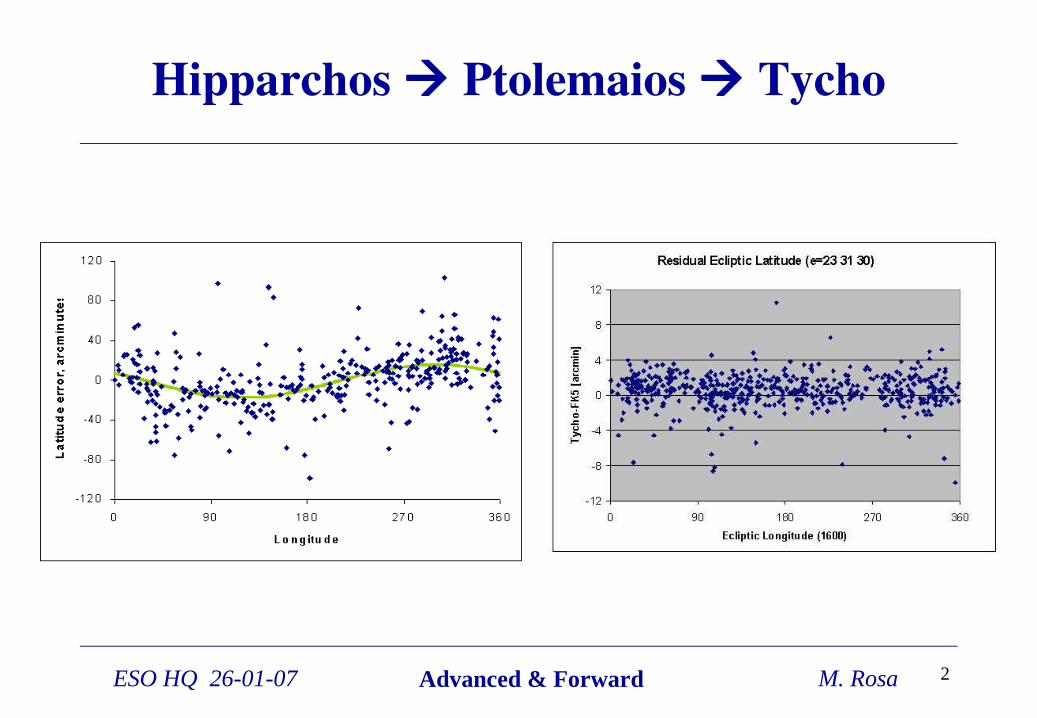
Hipparchos Ptolemaios Tycho
M. Rosa ESO HQ 26-01-07 Advanced & Forward 3
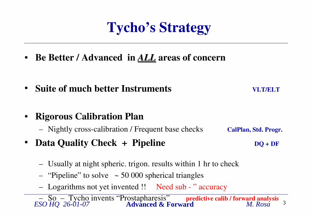
Tycho’s Strategy
• Be Better / Advanced in ALLALL areas of concern
• Suite of much better Instruments VLT/ELT
• Rigorous Calibration Plan– Nightly crosscalibration / Frequent base checks CalPlan, Std. Progr.
• Data Quality Check + Pipeline DQ + DF
– Usually at night spheric. trigon. results within 1 hr to check – “Pipeline” to solve ~ 50 000 spherical triangles – Logarithms not yet invented !! Need sub ” accuracy– So – Tycho invents “Prostapharesis” predictive calib / forward analysis

M. Rosa ESO HQ 26-01-07 Advanced & Forward 4
Agenda
• Key Points– Keeping the pace between upgrades of Scientific Aims (Ambitions) , Instrumentation and Methods– Consolidating ground conquered– Preparing for greater challenges
• Key Phrases Predictive Calibration & Forward Analysis– Predictive: utilizing physical (first) principles “a priory knowledge”– Forward: do justice to the (precious raw) “observables” by enabling
to map into and compare theoretical models of targets in the raw data domain

M. Rosa ESO HQ 26-01-07 Advanced & Forward 5
Heritage 1
• 1995 STECF / ESO Calibration WS– “Predictive Calibration based on Physical Instrument Models”
• In parallel ( 1998 ) ESO formulates– VLT Operations Plan Requirements for “Data Quality & Flow”
• 1997 1999 implementations of Physical Models– CASPEC + UVES (Ballester & Rosa 1977 theory paper)– UVES WCalib Bootstrap + more in ETCs (Ballester + team)– HST FOS (initially Rosa & Kerber)
• 1999 ESA Instrument Physical Modeling Group– thanks to former DG Riccardo Giacconi (see AnnRevAstrAstroph 2005)
M. Rosa ESO HQ 26-01-07 Advanced & Forward 6
Heritage 2
• 2000 2005 STECF Team on FOS & STIS – Alexov, Bristow, Fiorentino, Kerber, Rosa + contr. Modigliani (DMD)– FOS Post Operational Archive based on FOS model– STIS Model + SimulatedAnnealing demonstrated factor 10 +– Veryfied on superior entirely new PtNe/Cr line catalogue (NIST collab.)
• 2005/6 CRIRES / Xshooter model – Bristow + Kerber integrated into to ESOINS– thanks to DG Catherine Cesarsky (bringing them back from ESA)
• 2007 Physical Models established Instr. Support– Spectrograph kernel + Simulated Annealing ready to …– … support many more spectrographic instruments
M. Rosa ESO HQ 26-01-07 Advanced & Forward 7
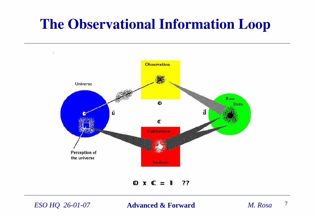
The Observational Information Loop
•
M. Rosa ESO HQ 26-01-07 Advanced & Forward 8
Demonstration Case
• HST Faint Object Spectrograph (FOS) – Relatively straight layout– Easy to grasp impact of “physical insight” on calibration– Obvious projection to FORSes …
• Case STIS (UVES, CRIRES, XShooter…)– More complex (2D – echelles, multiobjects…)– But also “done” (in principle …)
M. Rosa ESO HQ 26-01-07 Advanced & Forward 9
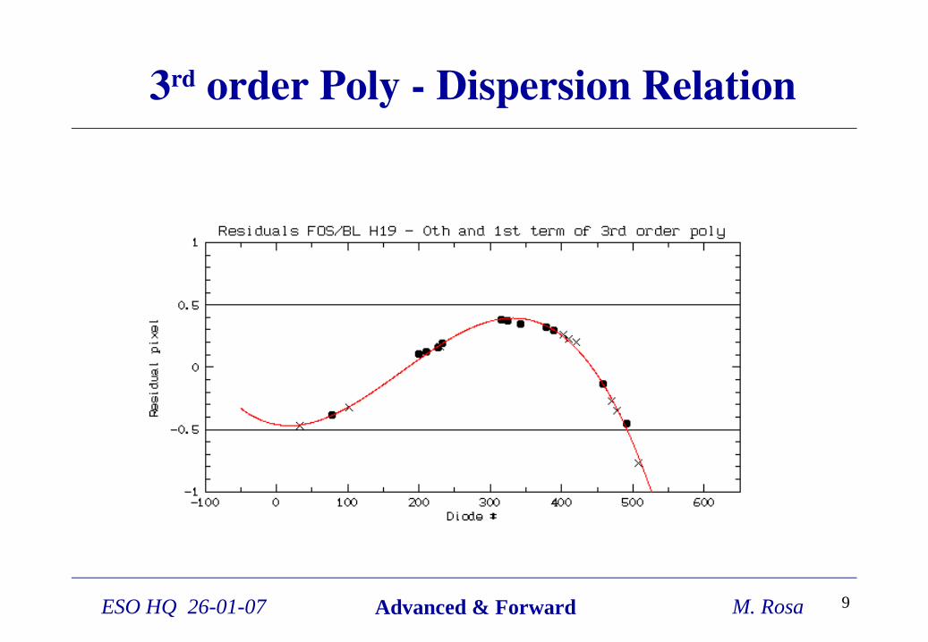
3rd order Poly Dispersion Relation
M. Rosa ESO HQ 26-01-07 Advanced & Forward 10
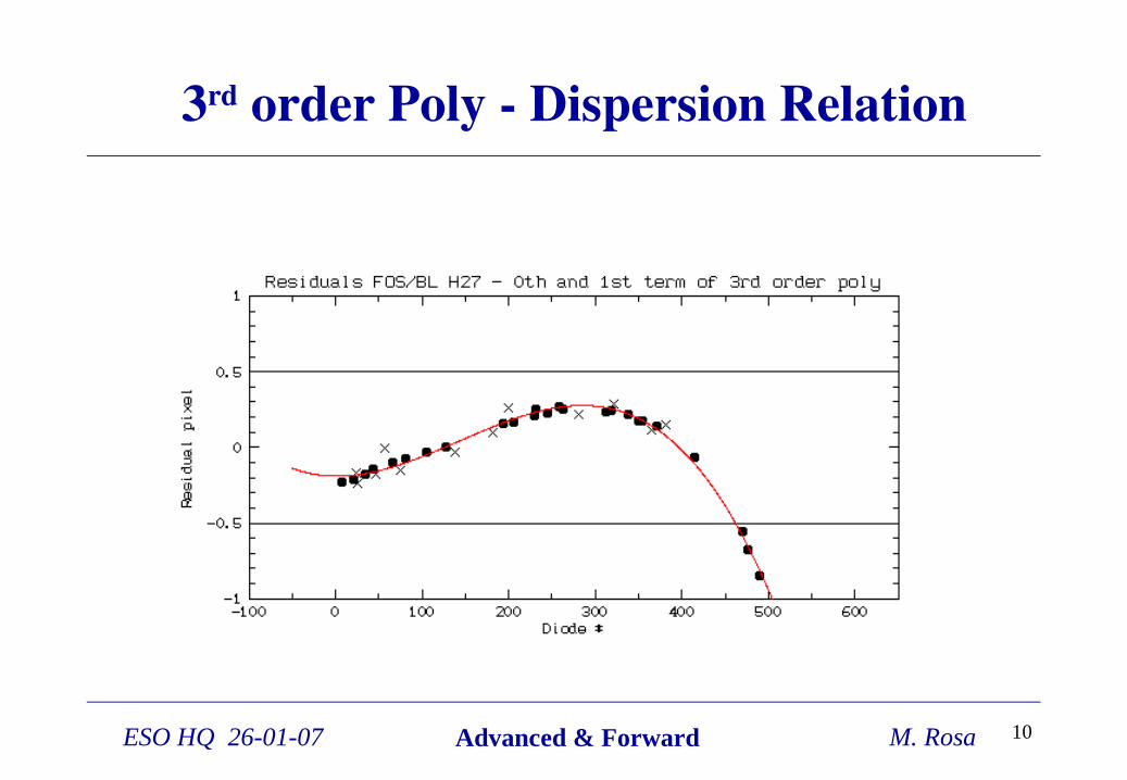
3rd order Poly Dispersion Relation
M. Rosa ESO HQ 26-01-07 Advanced & Forward 11
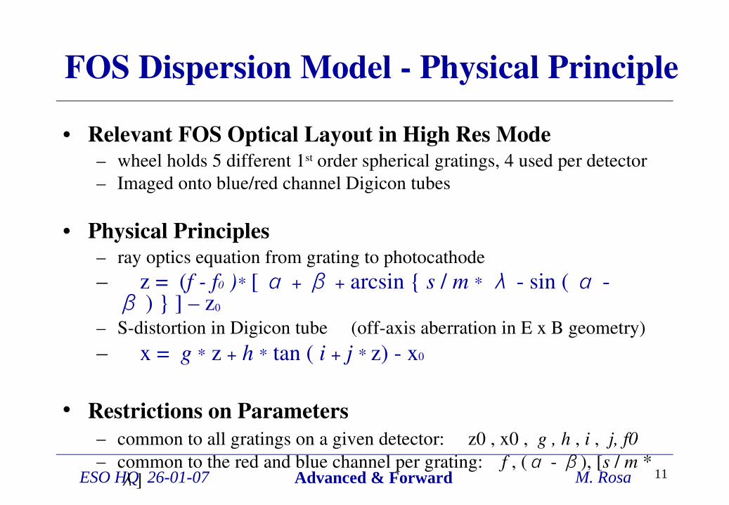
FOS Dispersion Model Physical Principle
• Relevant FOS Optical Layout in High Res Mode– wheel holds 5 different 1st order spherical gratings, 4 used per detector – Imaged onto blue/red channel Digicon tubes
• Physical Principles– ray optics equation from grating to photocathode– z = (f f0 )* [ α + β + arcsin { s / m * sin ( λ α
) } ] – zβ 0
– Sdistortion in Digicon tube (offaxis aberration in E x B geometry)– x = g * z + h * tan ( i + j * z) x0
• Restrictions on Parameters – common to all gratings on a given detector: z0 , x0 , g , h , i , j, f0– common to the red and blue channel per grating: f , ( ), [α β s / m *
] λ

M. Rosa ESO HQ 26-01-07 Advanced & Forward 12
FOS Dispersion Model
• Result (FOS BLUE)– Assume that SDistortion
common to the 3 clean library list modes valid for NUV/FUV as well
– Optimize common solution including the SDistortion
– Final residuals below 0.1 pix amplitude
– Common pattern to all modes is pincushion distortion

ESO HQ 26-01-07 Advanced & Forward 13
Dispersion Relations for FOS
• Shown are residuals measured w.r.t. model solution• FOS Dispersion Model valid for all gratings (differing colors)
– mode specific parameters: only grating constant, grating angle• Classical polynomial fit will fit all lines well
– whether or not they are blends, wrong identifications, too sparsely spread

M. Rosa ESO HQ 26-01-07 Advanced & Forward 14
Hipparchos Ptolemaios Tycho

ESO HQ 26-01-07 Advanced & Forward 15
MW Halo absorptions in QSO spectrum Standard “calfos”
• 2 long exposures (blk,red) show repeat error• Unphysical dependency of velocity on wavelength• Only one absorption at 1403 A seems to fit expectation
ESO HQ 26-01-07 Advanced & Forward 16
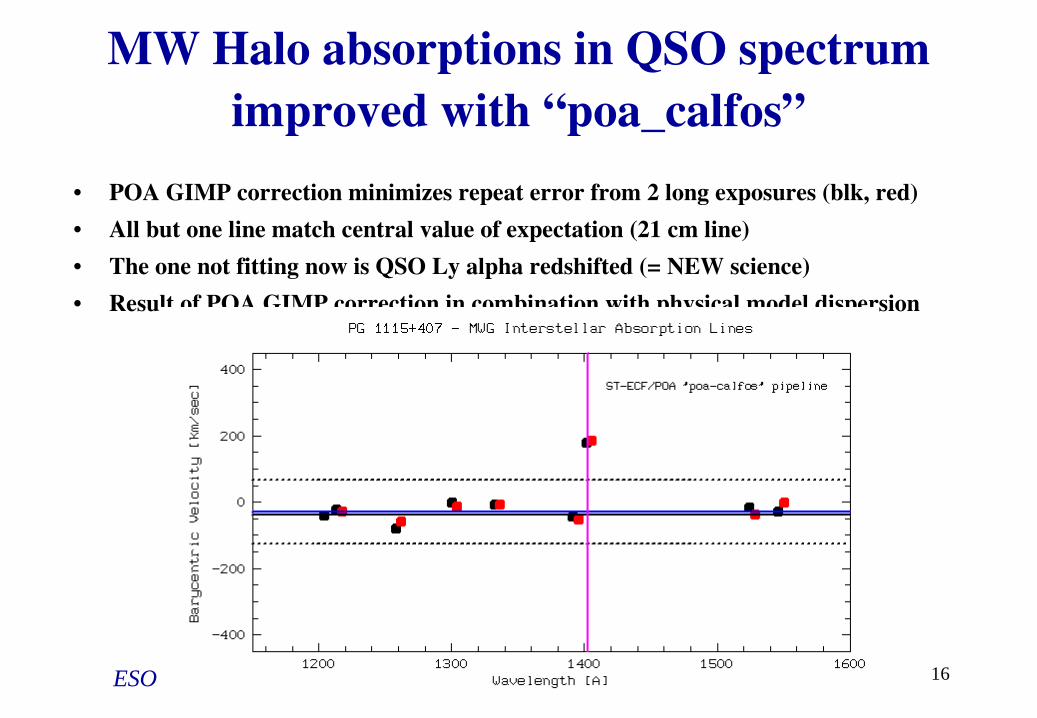
MW Halo absorptions in QSO spectrum improved with “poa_calfos”
• POA GIMP correction minimizes repeat error from 2 long exposures (blk, red)• All but one line match central value of expectation (21 cm line)• The one not fitting now is QSO Ly alpha redshifted (= NEW science)• Result of POA GIMP correction in combination with physical model dispersion

M. Rosa ESO HQ 26-01-07 Advanced & Forward 17
What about Flux Calibration • PM should only predict BlazeFunction
– Vignetting(s) will follow from optical path model– Mirror reflectivities etc. will enter as (accurate) laboratory measurables
but are allowed to change as required by insight (measurement)– Combined model will be tuned so that StdStar comes out correctly
• That is– PM predicts the SHAPE of the flux calib curve– SCALING is the business of onsky calibration ( zeropoints )

M. Rosa ESO HQ 26-01-07 Advanced & Forward 18
Grating Interference
M. Rosa ESO HQ 26-01-07 Advanced & Forward 19
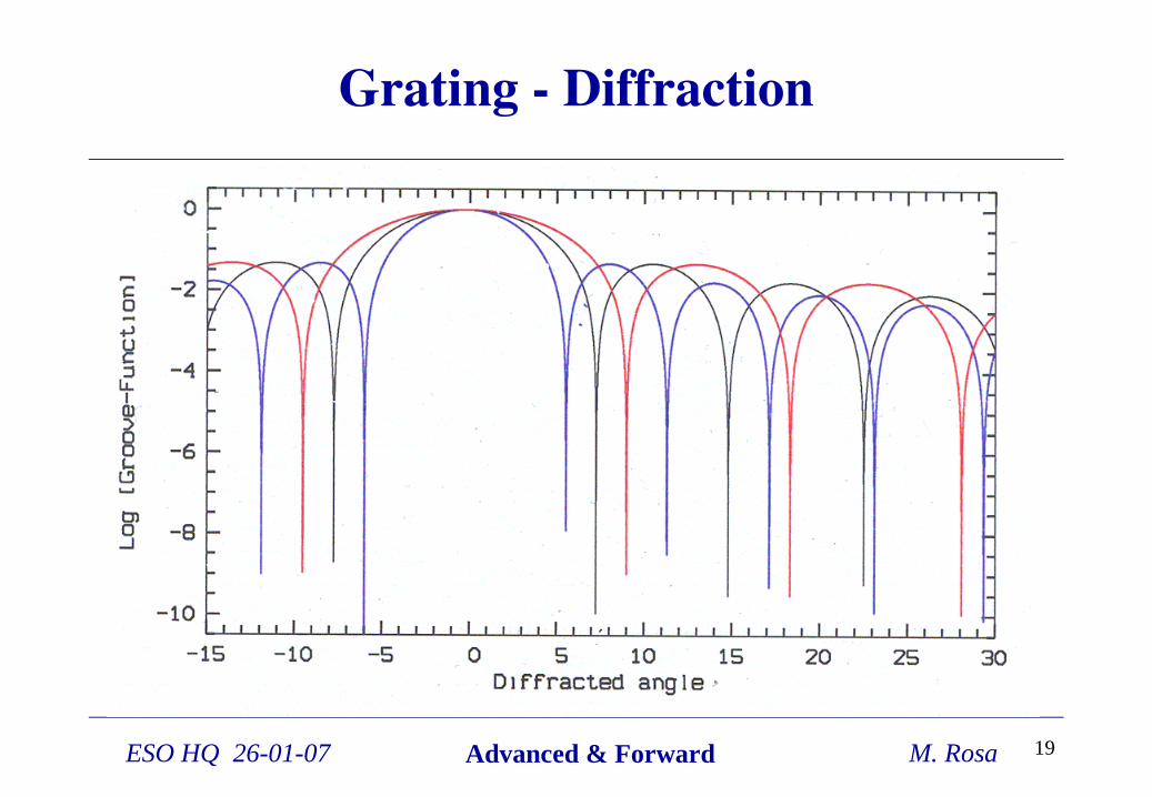
Grating Diffraction

M. Rosa ESO HQ 26-01-07 Advanced & Forward 20
IF * DF
M. Rosa ESO HQ 26-01-07 Advanced & Forward 21
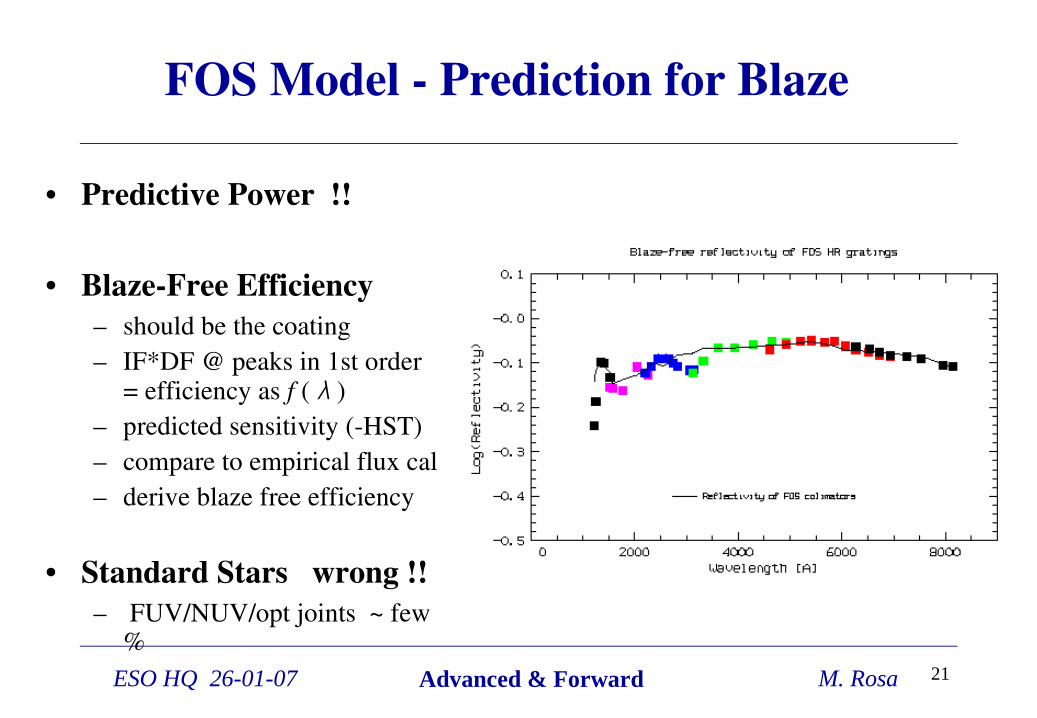
FOS Model Prediction for Blaze
• Predictive Power !!
• BlazeFree Efficiency – should be the coating– IF*DF @ peaks in 1st order
= efficiency as f ( )λ
– predicted sensitivity (HST)– compare to empirical flux cal– derive blaze free efficiency
• Standard Stars wrong !!– FUV/NUV/opt joints ~ few
%

M. Rosa ESO HQ 26-01-07 Advanced & Forward 22
Line Profile IF * DF (slit+collimator)

M. Rosa ESO HQ 26-01-07 Advanced & Forward 23
Line Profile obs vs theory (vign)

M. Rosa ESO HQ 26-01-07 Advanced & Forward 24
Line Profile obs vs theory (2)

M. Rosa ESO HQ 26-01-07 Advanced & Forward 25
Full Throughput Model Hot Target
M. Rosa ESO HQ 26-01-07 Advanced & Forward 26
Roadmap
• Very many “Observatory” pieces already in place – Cal Plans , DQC and data base– Know how of “how to deal with data” (extraction, peculiarities) – Build up of extensive data base on detector performance
• Know how, building blocks for “PhysModels” + Lab Standards
– many individuals already carry parts of the “company knowledge”– Parts of original IPMG integrated into ESOINS (Bristow, Kerber)– PhysMod based calibration part of CRIRES and XShooter Projects
• Required: Consolidation – Sustainability Development– Critical review of reference data and processes – Clearing station to achieve coherent view– Injection of advanced calibration concepts into instrument design
M. Rosa ESO HQ 26-01-07 Advanced & Forward 27
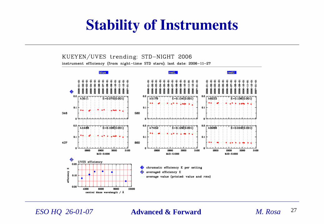
Stability of Instruments

M. Rosa ESO HQ 26-01-07 Advanced & Forward 28
Yes, agreed in principle, but …
• Nonstability of instruments on ground– PM strengths meaningful parameters insight– and see DQC trending eg. UVES, FORSes usually very stable
• On ground we have an atmosphere– PM strengths decoupling of instr. / atmosph. effects– Atmosphere becomes a separate “controllable” item
• Our instruments are too complicated– we designed them, so we have the insight– more complex more substantial insight helps
M. Rosa ESO HQ 26-01-07 Advanced & Forward 29
Atmosphere (terrestial)
• Key: Separate Instrumental Stuff from Atmosphere– Required: PhysMod based Calibration
• Atmosphere becomes another “model item”– At least from 320 to about 850 nm (the DoD knows that also beyond)– Extinction 34 components Form well known– Actual scaling should be controlled by LOSSAM / Std.Star expos
• Sky Brightness calls for a scaleable model as well F. Patat’s talk on Tuesday morning

M. Rosa ESO HQ 26-01-07 Advanced & Forward 30
Atmosphere (terrestial) cont.
• b.t.w. I’m proud that– everyone observing LS or PO is using “ATMOEXAN.TBL”– I constructed it in 1983 – by matching a 3 component Physical Model (Rayleigh, Ozone, Aerosols) … to the sparse data points of Tueg (1977 = Messenger 11)
• But– Anyone ever checked it for PO ? – it was for LS altitude !!– It does not include dust (Vulcanoes, CopperMining …)– Also, meanwhile we got “Globals” (Warming, Dimming etc …)

M. Rosa ESO HQ 26-01-07 Advanced & Forward 31
• So much for those that still pretend that
“ Physical Models can not be of much use at a ground based observatory …
… because we have an Atmosphere.
Michael you know, we prefer to use good old ATMOEXAN instead ”

M. Rosa ESO HQ 26-01-07 Advanced & Forward 32
Reminder: Observation Information Loop
•
M. Rosa ESO HQ 26-01-07 Advanced & Forward 33
Definitions & Examples
• First principle model Ray trace spectrograph model – prescription based entirely on physical laws – very high predictive power– required to isolate effects while building physical models
• Physical model UVES/STIS model (ray + dist.) – prescription primarily based on physical / engineering insight– empirical “fudge” only as unavoidable (tolerable) substitute– sufficient predictive power for predictive calibration, forward analysis
• Empirical model ETC, polyn. dispersion fits– no physical insight required / inserted , can not be inverted – no predictive power outside data range / when params change

M. Rosa ESO HQ 26-01-07 Advanced & Forward 34
FOS Scatter ModelTest on Data
• Recall– wanted to predict the observed
raw data for a cool target at UV wavelengths
– Test for a Solar Analog– pass Kurucz model of Sun
through the FOS model– compare with observations of
solar analog 16 Cyg B– @ 160 nm signal is 1% of
scattered (red) light– still the prediction agrees to
better 5 % with actual data
M. Rosa ESO HQ 26-01-07 Advanced & Forward 35
Concepts to Get Around the Info Loop
• Canonical Concept Empirical backward analysis Empirical backward analysis – empirical calibration relations rescale raw data interpretation
• Advanced Concept Predictive CalibrationPredictive Calibration – instrument models noise free calibration relations– first principles predictive capabilities outside “standards” range– Analysis: like empirical concept “backward” (scaled raw data)
• Superior Concept Forward AnalysisForward Analysis – can simulate raw data with sufficient accuracy and detail – evaluate theoretical target models in raw data domain– obtain likelihood estimates for range of potential target properties
M. Rosa ESO HQ 26-01-07 Advanced & Forward 36
Calibration in Context• Determine relation between output and the value of the input
quantity, a reference standard (ISO 9000) • Traceability – establish accuracy by an unbroken line to higher
standards. For each step evaluate uncertainty.• Quality Control – monitoring, stability • Data Reduction – or better “Preparation”
– removal of instrumental signatures, extraction, “resampling”
• Why do Calib and Reduc appear to be so intermingled ?
M. Rosa ESO HQ 26-01-07 Advanced & Forward 37
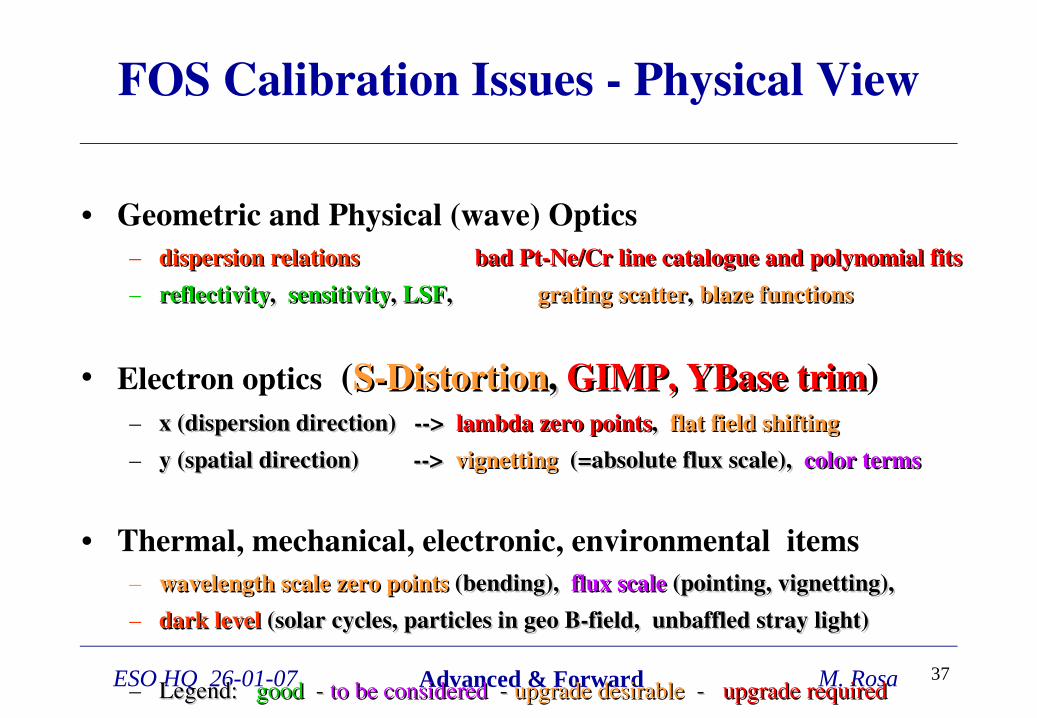
FOS Calibration Issues Physical View
• Geometric and Physical (wave) Optics– dispersion relations dispersion relations bad PtNe/Cr line catalogue and polynomial fitsbad PtNe/Cr line catalogue and polynomial fits – reflectivityreflectivity, , sensitivitysensitivity, , LSFLSF, , grating scattergrating scatter, , blaze functionsblaze functions
• Electron optics (SDistortionSDistortion, , GIMP, YBase trimGIMP, YBase trim) – x (dispersion direction) > x (dispersion direction) > lambda zero pointslambda zero points, , flat field shiftingflat field shifting– y (spatial direction) > y (spatial direction) > vignetting vignetting (=absolute flux scale), (=absolute flux scale), color termscolor terms
• Thermal, mechanical, electronic, environmental items– wavelength scale zero points wavelength scale zero points (bending), (bending), flux scale flux scale (pointing, vignetting), (pointing, vignetting), – dark level dark level (solar cycles, particles in geo Bfield, unbaffled stray light)(solar cycles, particles in geo Bfield, unbaffled stray light)
– Legend: Legend: good good to be consideredto be considered upgrade desirableupgrade desirable upgrade requiredupgrade required