from macro to wells & fields… agents behavior in energy

From Macro to Wells & Fields… Agents behavior in energy markets

International Association of Energy Economists

Montreal May-June, 2019

John W. Ballantine, Jr. PhD. Brandeis University

Mohammed AlMehdar, PhD candidate, Brandeis University

Not All Energy Agents Maximize Profits:Modelling Complexity of Investment in Oil & Gas Projects

With help from

Energy Agent Based Model,

NOT a profit maximizer

• The underlying premise of our approach is that an agent-based model (ABM) that uses a flexible structure can simulate market interactions and more particularly explain the investment and production cycles. In other words, energy producers have different investment / profit maximizing functions and the heterogeneity of agents investment matters.

• The investment, production, and cash flow actions of National Oil Companies, Independent Oil Companies and Shale producers, operating in fields with different costs affects energy supply and, of course, prices.

• Our agent based, fuzzy logic model lets us to run “what if” simulations by changing common language assumptions (e.g., behaviour rule: invest more in shale if prices are high/over $60 a barrel; expand low cost oil & gas fields if expected demand / price peaks in five years).

• By using field level data to estimate agent investment functions derived from heterogeneous profit expectations we explain the differences of oil production of individual agents and resulting market dynamics.

Large diversified O&G supplyClose to market, Many not

Politics and finance barriersWho manages JV projects & complicated supply chains

Unlimited low cost supplyStable opaque governance

Respond to market surprisesSometimes critical budget

balanceFew constraints, except location

Mature variable cost supplierMarkets close to supply chainCompetitive market players

Some win and some loseProfits, finance, value matter

Large high cost fieldsLong lead times, long lifeMany partners, less riskStable supply to markets

Cash flow matters

Heterogeneous Agents with Different geologies: Invest Differently with Different production paths that changes Market Dynamics, Prices Volatility

Heterogeneous Agents Affect Supply Curve

• Changing agent expectations / interactions and Investment actions

• Energy supply dynamics / feedback loops and price volatility

• Longer run investment decisions and oil & gas supply curve

Medium term

ENERGY PRICESand

Energy MIX

Individual / separate agent expectations &

investments

Government policy

actions

Oil & Gas Supply

> = <

Market Demand

Today’s Agenda:a work in progress

1. Problem / Challenge

2. Current Framework / Approach

3. Hypothesis, NOT NPV profit maximization

4. The Data: Field / Projects and Agents

5. Agents with Different Investment approaches

6. Preliminary ABM / Fuzzy Logic Workplan

7. Does it Matter? YES

The Problem and Challenges

What demand, What supply, What price?

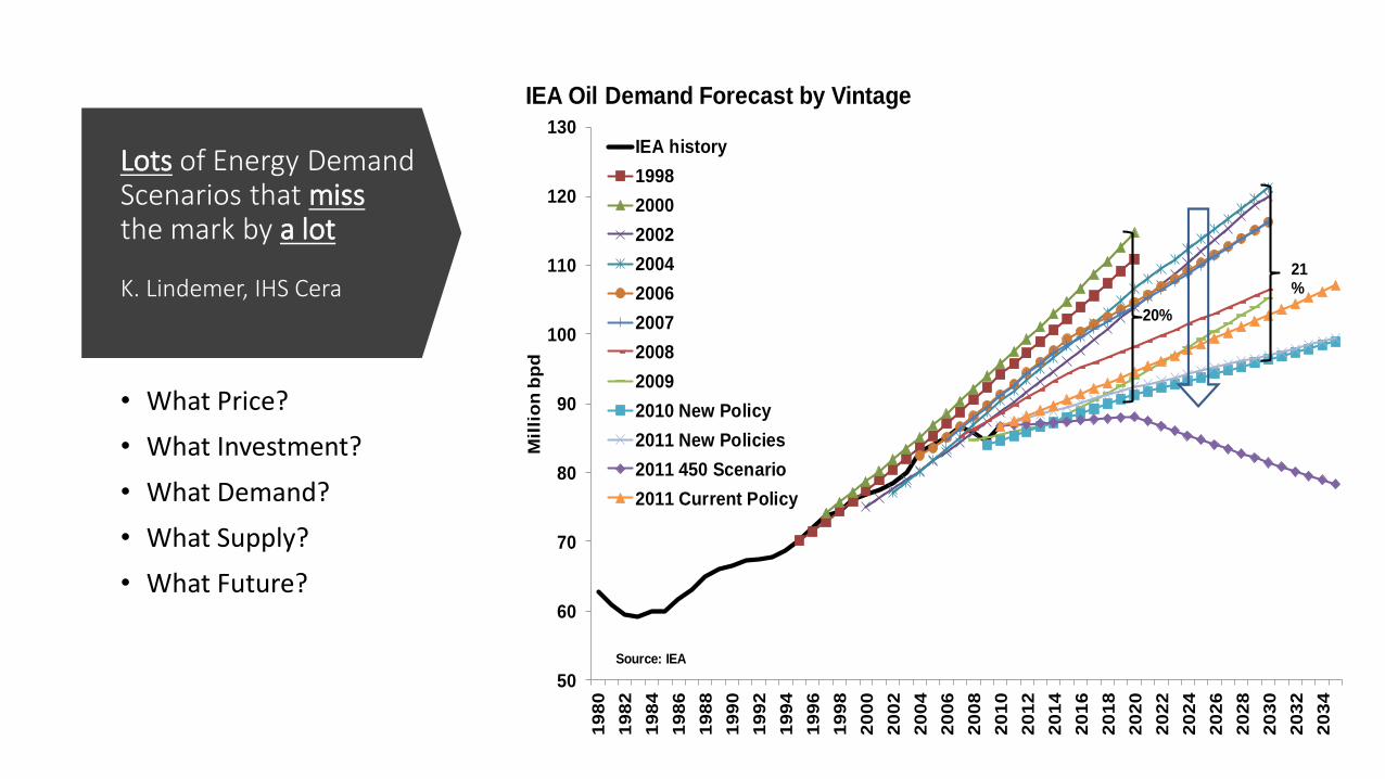
Lots of Energy Demand Scenarios that miss the mark by a lot

K. Lindemer, IHS Cera

• What Price?

• What Investment?

• What Demand?

• What Supply?

• What Future?

50

60

70

80

90

100

110

120

130

19

80

19

82

19

84

19

86

19

88

19

90

19

92

19

94

19

96

19

98

20

00

20

02

20

04

20

06

20

08

20

10

20

12

20

14

20

16

20

18

20

20

20

22

20

24

20

26

20

28

20

30

20

32

20

34

Mil

lio

n b

pd

IEA Oil Demand Forecast by Vintage

IEA history

1998

2000

2002

2004

2006

2007

2008

2009

2010 New Policy

2011 New Policies

2011 450 Scenario

2011 Current Policy

20%

21%

Source: IEA

Shifting Oil Supply

-5

-4

-3

-2

-1

0

1

2

3

4

5

2008 2009 2010 2011 2012 2013 2014

© 2014 IHS

Mill

ion

ba

rre

ls p

er

da

y

Net change for rest of

the world

Russia

Canada

US Total

Saudi Arabia

5.0

5.5

6.0

6.5

7.0

7.5

8.0

8.5

9.0

9.5

15

17

19

21

23

25

27

Millio

n b

arr

els

/da

y

Tri

llio

n c

ub

ic fe

et/

ye

ar

Natural gas Crude oil

Shale Boom

Cumulative change in crude oil production from 2008-2014 US shale production

IHS/Lindemer

Oil Price Forecasting… NOT a smooth trend line!

10

$0

$50

$100

$150

$200

$250

1970

1972

1974

1976

1978

1980

1982

1984

1986

1988

1990

1992

1994

1996

1998

2000

2002

2004

2006

2008

2010

2012

2014

2016

2018

2020

2022

2024

2026

2028

2030

2032

2034

2036

2038

2040

2014

$/b

bl

1979 1982 1983 1984 1985 1986 1987 1989 1990

1991 1992 1993 1994 1995 1996 1997 1998 1999

2000 2001 2002 2003 2004 2005 2006 2007 2008

2009 2010 2011 2012 2013 2014 2015 2016 Actual

Conventional wisdom of the day during the 1970s

Source: EIA

Price volatility: boom and bust

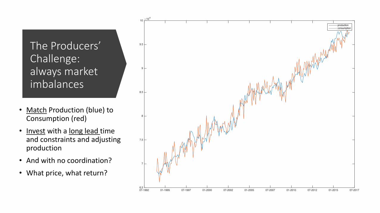
The Producers’ Challenge: always market imbalances

• Match Production (blue) to Consumption (red)

• Invest with a long lead time and constraints and adjusting production

• And with no coordination?

• What price, what return?

Current Frameworks &

Literature

Market Equilibrium and

Surprises & shocks

(IEA, Shell, BP, EIA… and Killian, et. al.. and

Oxford Energy Economics

General Equilibrium Macro Structure: Supply > = < Demand

IEA, EIA, OPEC, Shell ➔ huge data gathering and estimation

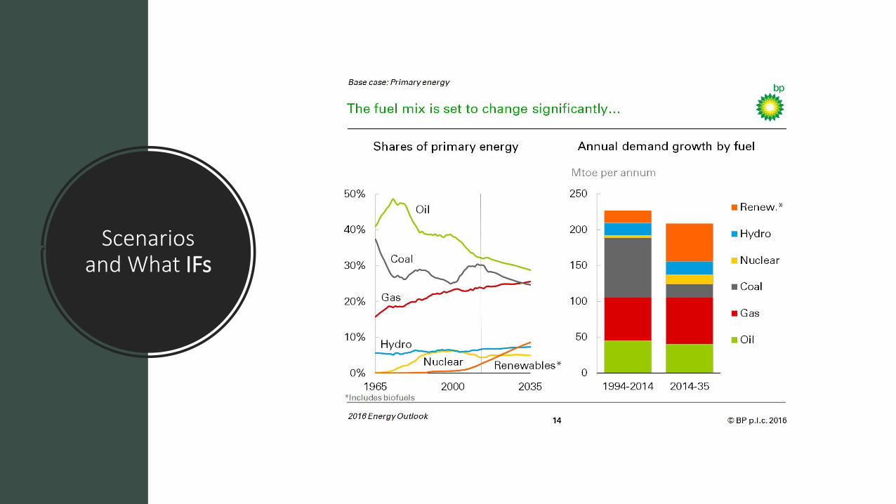
Scenarios and What IFs

Supply & Demand shocks (VAR models): World crude oil production in monthly percent changes, 1973 -2016

Exogenous disruptions and OPEC / Saudi Arabia as swing producer in thousand barrels per day, 1990-2016

Politics again and again and again: Iran, Russia, Ukraine, Venezuela,

Nigeria, Brazil, Qatar, Saudi Arabia, Israel, US, and …

Whys of Price

Volatility

Shocks,behavior,changed

expectation

Supply: Demand Stagflation IR up recession New fields on Asian FX crisis Asian growth Financial crisis Sanctions

Political tensions Yon Kippur Iran revolution Iran/Iraq, then Kuwait War

Russia Yeltsin, slow growth

9 / 11, Venezuela

IPCC climateRussia Crimea

Paris COP 15Iran/JCPOA

Technology Alaska pipeline North sea oil

Invest wind parity … solar

Shale fracking, Gulf rig explods

Horizonal drilling

Market players OPEC, longercontracts

Saudi Arabia increase oil

Opec cuts, cheating

OPEC quotas Saudi production

China gas pipelines

OPEC, Russia, Saudi, China

Limitations of these

approaches

• Simplified Shocks, Demand == Supply and Price Volatility models

• What short / long Price expectations?

• Supply chains matter with known bottlenecks (not surprises)

• Lags in investment, production, decline rates by region, fields,

• Endogenous actions of producers with different expectations

• Changing behavioral actions of producers / consumers

• Always politics and exogeneous producer surprises

• NPV of investment…Not necessarily true of for all

Heterogeneous producer model in non-equilibrium oil markets

Where to invest? What to Invest? When Returns?

NOT All Agents Maximize

Project NPV

Modeling Complexity of Agent Based Investment /

Production Behavior

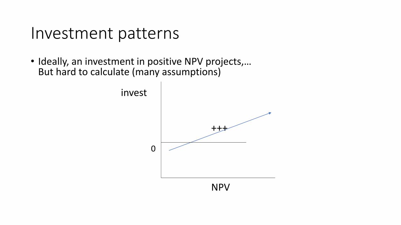
Investment patterns

• Ideally, an investment in positive NPV projects,…But hard to calculate (many assumptions)

invest

+++

0

NPV

The IHS / Vantage Field and Project Data

IHS data• Specific data of

• Discovery • Capex• Operating costs• Taxes / royalties

• Total costs • Production over time• Price and Barrels

Costs (real) and NPV calculations• Breakeven costs• Mean reversion • Revenue – costs = Cash flow

• P and Q history• Price assumptions• Discount rates• With and w/o taxes

• Oil & (Gas) and Shale• Production (Q) and Price (P) over

project life

Investment patterns / cycles

• Investment = F (costs/breakeven, quantity produced. NPV estimate, S:D balance, technology, and other factors, variables…)

• Sorting NPV and investment behavior (expected Price, Quantity, and NPV)

Quantity

H

L

Low High

Breakeven

HIGH NPV projects Lower NPV because of costs (deep water)

Lower potential and NPV due Q Not necessarily positive NPV,

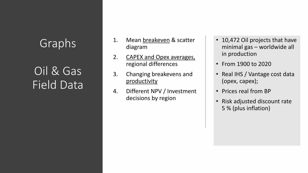
Graphs

Oil & Gas Field Data

1. Mean breakeven & scatter diagram

2. CAPEX and Opex averages,regional differences

3. Changing breakevens andproductivity

4. Different NPV / Investment decisions by region

• 10,472 Oil projects that have minimal gas – worldwide all in production

• From 1900 to 2020

• Real IHS / Vantage cost data (opex, capex);

• Prices real from BP

• Risk adjusted discount rate 5 % (plus inflation)

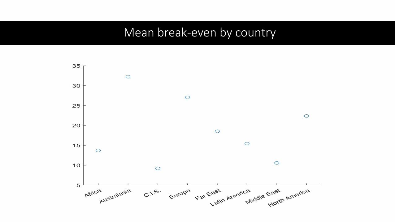
Mean break-even by country

Capex and Opex averages

Breakeven scatter

Breakeven costs by region – RED Invest, Blue No

Regions: Production, Capex, Opex

Cumulative Production

Distribution of reserves

NPV regions: PQ – costs (Red invest, blue no) rate

Regional NPV reversion to mean, logs

NPV values – mean reversion with taxes

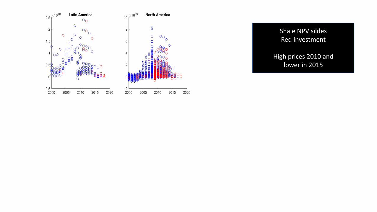
SHALE NPV Investment slides Shale NPV sildesRed investment

High prices 2010 and lower in 2015

Shale Mean Revision in logs wide dispersion:

many investment decisions. Why?

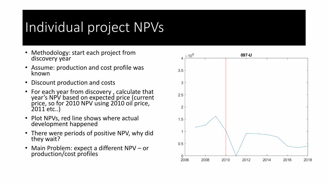
Individual project NPVs

• Methodology: start each project from discovery year

• Assume: production and cost profile was known

• Discount production and costs

• For each year from discovery , calculate that year’s NPV based on expected price (current price, so for 2010 NPV using 2010 oil price, 2011 etc..)

• Plot NPVs, red line shows where actual development happened

• There were periods of positive NPV, why did they wait?

• Main Problem: expect a different NPV – or production/cost profiles

Investment ➔ Production

-5

-4

-3

-2

-1

0

1

2

3

4

5

2008 2009 2010 2011 2012 2013 2014

© 2014 IHS

Mill

ion

ba

rre

ls p

er

da

y

Net change for rest of

the world

Russia

Canada

US Total

Saudi Arabia

Cumulative change in crude oil production from 2008-2014

IHS/Lindemer

ComparingOIL & Gas NPV Projects and Shale

NOT All Agents

Invest to Maximize NPV?

• Agents act differently

• Different investment and production behaviors

• Different expectations and NPVs

• QED

Modeling Complexity in

Oil Markets

Why Agents Matter

&

How Invest

Our Agent-based Fuzzy Logic Approach

Building Producer module in Agent Based System

How Build Agent Based Model?

Complexity in Energy Markets:

• Stylized facts don’t fit!

• Agent changes in investment and supply

Use Agent-Based Methodology

• Realism & Flexibility

• Medium range market dynamics

Need for different modelling paradigm

• Modular to deal with different features

• Applies with uncertain/noisy data

• Highly non-linearinteractions with feedback loops

Russia and CISLarge diversified O&G supply

Close to market, Many notPolitics and finance barriersWho manages JV projects & complicated supply chains

MENA CountriesUnlimited low cost supplyStable opaque governance

Respond to market surprisesSometimes critical budget balance

Few constraints, except location

Non OPEC producersMature variable cost supplierMarkets close to supply chainCompetitive market players

Some win and some loseProfits, finance, value matter

Off-ShoreLarge high cost fields

Long lead times, long lifeMany partners, less riskStable supply to markets

Cash flow matters

Heterogeneous Oil & Gas Agents – how many? 4-5?

US ShaleLow cost and short

timeframes

Price &

Quantity

Possible Agents and Behaviors

Simplified agent / regions

• National Oil Companies• Independent Oil Companies• OPEC and Saudi Arabia• Russia• Shale Producers

Differentiated agent behavior

• Geology (IHS data available)- production- decline rate- investment- reserves

• Financial (many gaps)- price- costs- cash flow (profits)- fiscal deficit / other- expectations

• other

Are agents so different?(IHS well / field data)

0

5000

10000

15000

20000

25000

19

70

19

72

19

74

19

76

19

78

19

80

19

82

19

84

19

86

19

88

19

90

19

92

19

94

19

96

19

98

20

00

20

02

20

04

20

06

20

08

20

10

20

12

20

14

20

16

20

18

20

20

20

22

20

24

20

26

'00

0 b

pd

Oil Production from Selected Regions

'C.I.S.' 'Onshore' 'Middle East' 'Onshore' 'North America' 'Onshore'

0

5000

10000

15000

20000

25000

30000

Capital Development Spending (MMUSD)

'C.I.S.' 'Onshore' 'Middle East' 'Onshore/Offshore' 'North America' 'Onshore'

Are agents so different?(productivity and investment cycles)

0

1

2

3

4

5

6

7

8

9

19

70

19

72

19

74

19

76

19

78

19

80

19

82

19

84

19

86

19

88

19

90

19

92

19

94

19

96

19

98

20

00

20

02

20

04

20

06

20

08

20

10

20

12

20

14

20

16

Capital/Production


0

2000

4000

6000

8000

10000

12000

19

70

19

72

19

74

19

76

19

78

19

80

19

82

19

84

19

86

19

88

19

90

19

92

19

94

19

96

19

98

20

00

20

02

20

04

20

06

20

08

20

10

20

12

20

14

20

16

Capital Spending per Year (adjusted for PPI)


Agent Cash Flow to Invest?(Revenue – costs = Free cash flow – capex)

0

1E+11

2E+11

3E+11

4E+11

5E+11

6E+11

7E+11

19

70

19

71

19

72

19

73

19

74

19

75

19

76

19

77

19

78

19

79

19

80

19

81

19

82

19

83

19

84

19

85

19

86

19

87

19

88

19

89

19

90

19

91

19

92

19

93

19

94

19

95

19

96

19

97

19

98

19

99

20

00

20

01

20

02

20

03

20

04

20

05

20

06

20

07

20

08

20

09

20

10

20

11

20

12

20

13

20

14

20

15

20

16

20

17

.00

Reconstructed Revenue (Oil Price * Production)


Geology of Fields

and Agent Behavior

• Invest IF Price over $50 a barrel….for xx years

• Invest IF $$ finance available and JV partners

• Produce More IF Price over $60 a barrel and Inventories low

• Hold production stable - Invest as fields decline

• Produce more IF deficits grow

• ….

NEXT Our Simulated Agent Behaviors &

Interactions

from macro to wells & fields… agents behavior in energy

Documents