from linear to convex systems: consistency, farkas™ lemma

From linear to convex systems: Consistency, Farkas�

Lemma and applications�

N. Dinhy, M.A. Gobernazand M.A. Lópezx

June 6, 2005 (revised version)

Abstract

This paper analyzes inequality systems with an arbitrary number of proper lower

semicontinuous convex constraint functions and a closed convex constraint subset of a

locally convex topological vector space. More in detail, starting from well-known results

on linear systems (with no constraint set), the paper reviews and completes previous

works on the above class of convex systems, providing consistency theorems, two new

versions of Farkas� lemma, and optimality conditions in convex optimization. A new

closed cone constraint quali�cation is proposed. Suitable counterparts of these results

for cone-convex systems are also given.

1 Introduction

This paper mainly deals with systems of the form

� := fft(x) � 0; t 2 T ; x 2 Cg;

where T is an arbitrary (possibly in�nite) index set, C � X, X is a locally convex Hausdor¤

topological vector space, and ft : X ! R [ f+1g for all t 2 T . We assume that � satis�esthe following mild condition:

�This research was partially supported by MCYT of Spain and FEDER of EU, Grant BMF2002-04114-

C02-01.yDepartment of Mathematics-Informatics, Ho Chi Minh city University of Pedagogy, HCM city, Vietnam.

Work of this author was partly carried out while he was visiting the Department of Statistics and Operations

Research, University of Alicante, Spain, to which he is gratefull to the hospitality received.zDepartment of Statistics and Operations Research, University of Alicante, Spain.xDepartment of Statistics and Operations Research, University of Alicante, Spain.

1

brought to you by COREView metadata, citation and similar papers at core.ac.uk

provided by Repositorio Institucional de la Universidad de Alicante

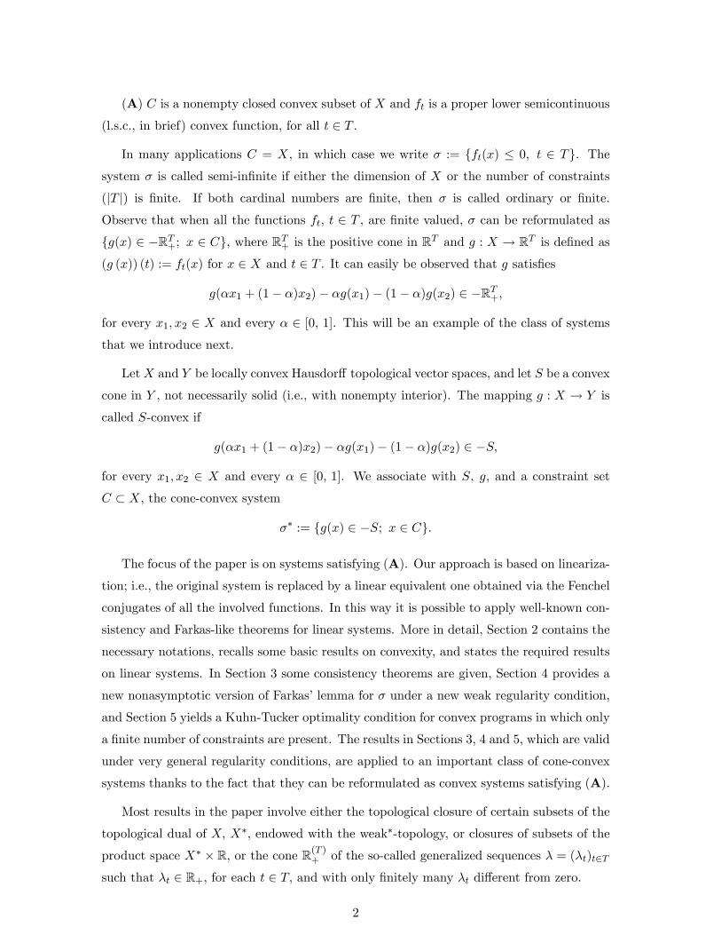
https://core.ac.uk/display/16361428?utm_source=pdf&utm_medium=banner&utm_campaign=pdf-decoration-v1

(A) C is a nonempty closed convex subset of X and ft is a proper lower semicontinuous

(l.s.c., in brief) convex function, for all t 2 T .

In many applications C = X, in which case we write � := fft(x) � 0; t 2 Tg. Thesystem � is called semi-in�nite if either the dimension of X or the number of constraints

(jT j) is �nite. If both cardinal numbers are �nite, then � is called ordinary or �nite.

Observe that when all the functions ft, t 2 T , are �nite valued, � can be reformulated asfg(x) 2 �RT+; x 2 Cg, where RT+ is the positive cone in RT and g : X ! RT is de�ned as

(g (x)) (t) := ft(x) for x 2 X and t 2 T . It can easily be observed that g satis�es

g(�x1 + (1� �)x2)� �g(x1)� (1� �)g(x2) 2 �RT+;

for every x1; x2 2 X and every � 2 [0; 1]. This will be an example of the class of systemsthat we introduce next.

LetX and Y be locally convex Hausdor¤ topological vector spaces, and let S be a convex

cone in Y , not necessarily solid (i.e., with nonempty interior). The mapping g : X ! Y is

called S-convex if

g(�x1 + (1� �)x2)� �g(x1)� (1� �)g(x2) 2 �S;

for every x1; x2 2 X and every � 2 [0; 1]. We associate with S, g; and a constraint setC � X, the cone-convex system

�� := fg(x) 2 �S; x 2 Cg:

The focus of the paper is on systems satisfying (A). Our approach is based on lineariza-

tion; i.e., the original system is replaced by a linear equivalent one obtained via the Fenchel

conjugates of all the involved functions. In this way it is possible to apply well-known con-

sistency and Farkas-like theorems for linear systems. More in detail, Section 2 contains the

necessary notations, recalls some basic results on convexity, and states the required results

on linear systems. In Section 3 some consistency theorems are given, Section 4 provides a

new nonasymptotic version of Farkas�lemma for � under a new weak regularity condition,

and Section 5 yields a Kuhn-Tucker optimality condition for convex programs in which only

a �nite number of constraints are present. The results in Sections 3, 4 and 5, which are valid

under very general regularity conditions, are applied to an important class of cone-convex

systems thanks to the fact that they can be reformulated as convex systems satisfying (A).

Most results in the paper involve either the topological closure of certain subsets of the

topological dual of X; X�, endowed with the weak�-topology, or closures of subsets of the

product space X� � R, or the cone R(T )+ of the so-called generalized sequences � = (�t)t2T

such that �t 2 R+; for each t 2 T; and with only �nitely many �t di¤erent from zero.

2

2 Preliminaries

For a set D � X; the closure of D will be denoted clD. The convex hull of D will be

represented by convD; and the convex cone generated by D[f0g by coneD. In the sequel,and for the sake of convenience, the closure with respect to the weak�-topology of a subset

A of the dual space X� will be denoted by clA as well (which specially makes sense when

A is convex).

Let further I be an arbitrary index set, fXi; i 2 Ig be a family of subsets of X, and let= be the collection of all the nonempty �nite subsets of I. Then

cone

[i2IXi

!=[J2=

cone

0@[j2J

Xj

1A =[J2=

0@Xj2J

coneXj

1A : (1)

Lemma 2.1 Let A be a nonempty subset of X and let B be a convex cone of X containing

the vector zero. Then

cone(A+B) � cone(A [B) � cl cone(A+B): (2)

Proof. We have to prove only the second inclusion. Since 0 2 B, A � A + B. It remainsto be proved that B � cl cone(A+B). Let b 2 B. If we take an arbitrary a 2 A, and fromthe assumption on B, a+nb 2 A+B for any n 2 N. It follows that n�1a+ b 2 cone(A+B)for any n 2 N. Letting n!1 we get b 2 cl cone(A+B). �

It is worth noting, from (2), that if cone(A+B) is closed then cone(A[B) = cone(A+B)is closed. The converse is not true as the following simple example shows.

Example 2.1 Let X = R2, B = f0g�R+, and A = f1g�R+. Then cone(A[B) = R2+is closed whereas cone(A+B) = (R++ � R+)[f(0; 0)g, which is not a closed subset of R2+.

For a nonempty closed convex set C in X; the recession cone of C; denoted by C1; is

de�ned in [17] as

C1 :=\">0

"cl[

0<�<"

�C

#;

where �C := f�c j c 2 Cg: According to [17, Theorem 2A], C1 can be characterized

algebraically as

C1 = fz 2 X j C + z � Cg

=

8<:z 2 X�� there exists some c 2 C such thatc+ �z 2 C for every � � 0

9=;= fz 2 X j c+ �z 2 C for all c 2 C and every � � 0g :

(3)

3

For a set D � X; the indicator function �D is de�ned as �D(x) = 0 if x 2 D and

�D(x) = +1 if x =2 D. If D is nonempty, closed and convex, then �D is a proper l.s.c.

convex function. The normal cone of D at x is given by

ND (x) = fu 2 X� j u (y � x) � 0 for all y 2 Dg ;

when x 2 D, and ND (x) = ?, otherwise.

Now let f : X ! R [ f+1g be a proper l.s.c. convex function. The e¤ective domain,the graph, and the epigraph of f are

dom f = fx 2 X j f(x) < +1g;

gphf = f(x; f (x)) 2 X � R j x 2 dom fg ;

and

epi f = f(x; ) 2 X � R j x 2 dom f; f(x) � g;

respectively, whereas the conjugate function of f; f� : X� ! R [ f+1g, is de�ned by

f�(v) = supfv(x)� f(x) j x 2 dom fg:

In particular, it is obvious that the support function of D � X is the conjugate of the

indicator function of D; and

��D (u) = ��cl(convD) (u) = sup

x2Du(x); u 2 X�:

It is well-known that f� is also a proper l.s.c. convex function and its conjugate, denoted

by f��, coincides with f . We also de�ne the subdi¤erential of f at x 2 dom f as

@f (x) = fu 2 X� j f (y) � f (x) + u (y � x) 8y 2 Xg ;

and the recession function of f; denoted by f1; as the proper l.s.c. sublinear function

verifying

epi f1 = (epi f)1:

For z 2 X and � 2 R; (3) gives rise to the following equivalence:

f1(z) � �, f(x+ �z) � f(x) + ��; for all x 2 X and all � � 0:

Thus, as a consequence of the so-called property of increasing slopes of the convex functions,

we have

f1(z) � �, sup�>0

f(x+ �z)� f(x)�

= lim�!1

f(x+ �z)� f(x)�

� �; for all x 2 X;

4

so that

f1(z) = lim�!1

f(x+ �z)� f(x)�

; for all x 2 X:

Hence

fz 2 X j f1(z) � 0g = fx 2 X j f(x) � �g1; (4)

for every � such that the lower sublevel set fx 2 X j f(x) � �g is nonempty. Consequently,f has bounded lower sublevel sets when fz 2 X j f1(z) � 0g = f0g and dimX < 1; butthis statement is no longer true in the in�nite-dimensional setting. Moreover, [17, Corollary

3D] establishes the following useful identity

f1 = ��cl(domf�): (5)

The following lemma was established in [3, Theorem 3.1] for proper l.s.c. convex func-

tions de�ned on a Banach space. However, the result still holds for locally convex vector

spaces without any change in the proof.

Lemma 2.2 (Convex subdi¤erential sum formulae). Let g; h : X ! R [ f+1g be properl.s.c. convex functions. If epig� + epih� is weak�-closed then for each a 2 domg \ domh,

@(g + h)(a) = @g(a) + @h(a):

It is worth noting that the conclusion of Lemma 2.2 still holds if one of the functions g

or h is continuous at one point in domg \ domh. In fact, if, for instance, g is continuous atc 2 domg, it is clear that c 2 int(domg) \ domh, and this implies 0 2 core(domg � domh);which, in turn, entails that cone(domg � domh) is a closed space. It then follows from [3,

Proposition 3.1] that the set epig� + epih� is weak�-closed.

Finally, in this introduction, we consider linear systems of the form

� := fat(x) � bt; t 2 Tg;

where at 2 X� and bt 2 R, for all t 2 T (observe that � satis�es condition (A), with C = X).We say that the system � is consistent if there exists z 2 X satisfying all the inequalities

in �. If � is consistent, an inequality a(x) � b, a 2 X� and b 2 R, is a consequence of � ifa(z) � b for all z 2 X solution of �. Now we recall two well-known results characterizing

the consistency and the consequent inequalities of � in terms of (at; bt) 2 X � R, t 2 T:

Lemma 2.3 (Consistency theorem). The following statements are equivalent to each other :

(i) � = fat(x) � bt; t 2 Tg is consistent ;(ii) (0;�1) =2 cl cone f(at; bt); t 2 Tg ;(iii) cl cone f(at; bt); t 2 T ; (0; 1)g 6= cl cone fat; t 2 Tg � R:

5

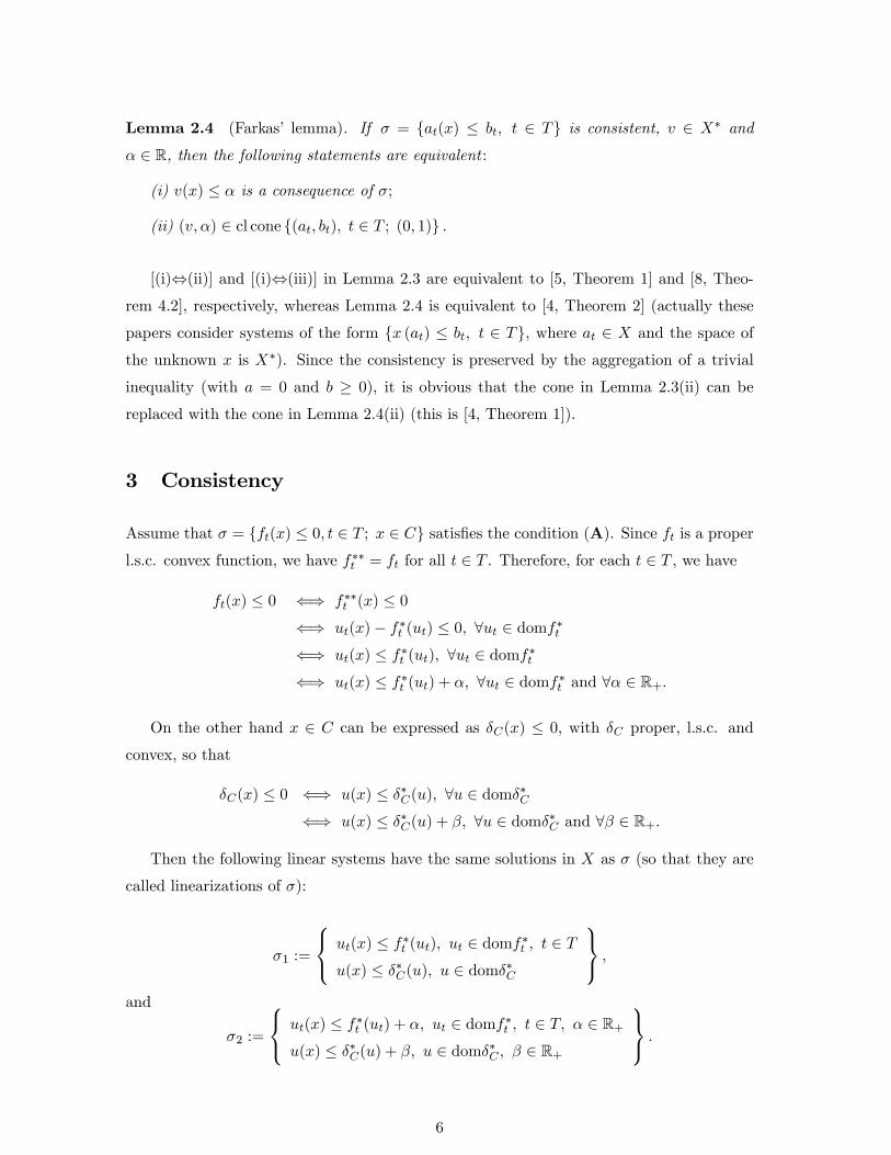
Lemma 2.4 (Farkas� lemma). If � = fat(x) � bt; t 2 Tg is consistent, v 2 X� and

� 2 R, then the following statements are equivalent :

(i) v(x) � � is a consequence of �;

(ii) (v; �) 2 cl cone f(at; bt); t 2 T ; (0; 1)g :

[(i),(ii)] and [(i),(iii)] in Lemma 2.3 are equivalent to [5, Theorem 1] and [8, Theo-

rem 4.2], respectively, whereas Lemma 2.4 is equivalent to [4, Theorem 2] (actually these

papers consider systems of the form fx (at) � bt; t 2 Tg, where at 2 X and the space of

the unknown x is X�). Since the consistency is preserved by the aggregation of a trivial

inequality (with a = 0 and b � 0), it is obvious that the cone in Lemma 2.3(ii) can be

replaced with the cone in Lemma 2.4(ii) (this is [4, Theorem 1]).

3 Consistency

Assume that � = fft(x) � 0; t 2 T ; x 2 Cg satis�es the condition (A). Since ft is a properl.s.c. convex function, we have f��t = ft for all t 2 T . Therefore, for each t 2 T , we have

ft(x) � 0 () f��t (x) � 0() ut(x)� f�t (ut) � 0; 8ut 2 domf�t() ut(x) � f�t (ut); 8ut 2 domf�t() ut(x) � f�t (ut) + �; 8ut 2 domf�t and 8� 2 R+:

On the other hand x 2 C can be expressed as �C(x) � 0, with �C proper, l.s.c. and

convex, so that

�C(x) � 0 () u(x) � ��C(u); 8u 2 dom��C() u(x) � ��C(u) + �; 8u 2 dom��C and 8� 2 R+:

Then the following linear systems have the same solutions in X as � (so that they are

called linearizations of �):

�1 :=

8<: ut(x) � f�t (ut); ut 2 domf�t ; t 2 Tu(x) � ��C(u); u 2 dom��C

9=; ;and

�2 :=

8<: ut(x) � f�t (ut) + �; ut 2 domf�t ; t 2 T; � 2 R+u(x) � ��C(u) + �; u 2 dom��C ; � 2 R+

9=; :

6

Theorem 3.1 Let � = fft(x) � 0; t 2 T ;x 2 Cg be a convex system satisfying condition

(A). Then the following statements are equivalent to each other :

(i) � is consistent ;

(ii) (0;�1) =2 cl cone�S

t2T gphf�t [ gph��C

;

(iii) (0;�1) =2 cl cone�S

t2T epif�t [ epi��C

;

(iv) cl cone�S


6= cl cone

�St2T domf

�t [ dom��C

� R:

Proof. The equivalence between (i) and (ii) is straightforward consequence of [(i)()(ii)]in Lemma 2.3, taking into account that the set of coe¢ cient vectors of �1 is

f(ut; f�t (ut)); ut 2 domf�t ; t 2 T ; (u; ��C(u)); u 2 dom��Cg =[t2T

gphf�t [ gph��C :

Now observe that the set of coe¢ cient vectors of �2 is

f(ut; f�t (ut) + �); ut 2 domf�t ; t 2 T; � � 0; (u; ��C(u) + �); u 2 dom��C ; � � 0g=St2T epif

�t [ epi��C :

Hence, by the same argument as before, � is consistent if and only if

(0;�1) =2 cl cone([t2T

epif�t [ epi��C

);

so that [(i)()(iii)] holds.

Finally, [(i)()(iv)] follows from [(i)()(iii)] in Lemma 2.3, applied to �1, taking intoaccount the identity

cone

"[t2T

gphf�t [ gph��C [ f(0; 1)g#= cone

([t2T


): � (6)

Observe that, according to Lemma 2.1 (since epi��C is a convex cone containing zero),

we have

cone

([t2T

epif�t + epi��C

)� cone

([t2T


); (7)

and

cl cone

([t2T


)= cl cone

([t2T


): (8)

>From (8), it is possible to replace, in statements (iii) and (iv) of Theorem 3.1,

cone�S


with cone

�St2T epif

�t + epi�

�C

. In particular, if C = X = Rn,

then epi��C = f0g � R+ and [(i)()(iii)] means that � = fft(x) � 0; t 2 Tg is consistent ifand only if

(0;�1) =2 cl cone([t2T

epif�t [ (f0g � R+))= cl cone

[t2T

epif�t

!

7

(this is [6, Proposition 3.1]). Similarly, from [(i)()(ii)], it is easy to prove that, if C = X,then � = fft(x) � 0; t 2 Tg is consistent if and only if (0;�1) =2 cl cone

�St2T gphf

�t

�(this

is [9, Theorem 3]).

We have observed that, if K is either

cone

([t2T

gphf�t [ gph��C

)or cone

([t2T


);

then

fv (x) � �; (v; �) 2 Kg

is a linearization of �. The same is true for

cone

([t2T


);

by (7), (8), and Lemma 2.4. These assertions come from the fact that the aggregation

of constraints which are consequent relations of a consistent system does not modify its

solution set.

The following results involve two desirable properties of � = fft(x) � 0; t 2 T ;x 2 Cgand a certain convex cone, K � X��R, such that fv (x) � �; (v; �) 2 Kg is a linearizationof �:

(C) K is weak�-closed;

(D) K is solid if X is in�nite dimensional, and

C1 \ fx 2 X j f1t (x) � 0; t 2 Tg = f0g: (9)

Notice that, by (7) and (8), if (C) holds for cone�S

t2T epif�t + epi�

�C

, then it also

holds for cone�S


, but the converse statement is not true; i.e., the closed

cone constraint quali�cation (C) is strictly weaker for cone�S


.

Example 3.1 Consider C = X = R and � = ff (x) = x � 0g. Then f� = �f1g and

��C = �f0g, so that (C) holds for cone�S


whereas it fails for

cone�S


�C

(recall Example 2.1). On the other hand, since C1 = R and

f1 (x) = x, we have fx 2 C1 j f1(x) � 0g = ]�1; 0] 6= f0g so that (D) cannot holdindependently of K.

Concerning the couple of cones formed by cone�S


and

cone�S


, we can have that (C) holds for exactly one of them. The fol-

lowing example shows the nontrivial part of this statement.

8

Example 3.2 Consider C = X = R2 and the inconsistent system

� =�ft (x) = tx1 + t

2x2 + 1 � 0; t 2 [�1; 1]:

Then

cone

([t2T


)= cone

��t; t2;�1

�; t 2 [�1; 1]

is closed whereas

cone

([t2T


)= cone

"[t2T

gphf�t [ gph��C [ f(0; 0; 1)g#

is not closed, so that (C) holds for cone�S


but not for

cone�S


. Let us observe that (D) also fails since

fx 2 C1 j f1t (x) � 0; t 2 [�1; 1]g =�x 2 C1 j tx1 + t2x2 � 0; t 2 [�1; 1]

= f0g � ]�1; 0] :

It is worth noting that the system in Example 3.2 is inconsistent. The following propo-

sition shows that if � is consistent and (C) holds for cone�S


, then it

also holds for cone�S


.

Proposition 3.1 If � is consistent and cone�S


is weak�-closed, then

cone�S


is also weak�-closed.

Proof. In fact, since (0;�1) =2 cone�S


, this cone being weak�-closed

by hypothesis, and since cone f(0; 1)g is weak�-closed and locally compact (because it is�nite-dimensional) and (6) holds, we get the conclusion from the well-known Dieudonné

theorem (see, for instance, [21, Theorem 1.1.8]). �

The regularity condition (C), with K := cone�S


�C

, was introduced

in [13] for the case where X is a Banach space and all the functions involved are �nite

valued, and it is called the closed cone constraint quali�cation. It is worth emphasizing

that this regularity condition is strictly weaker than several known interior type regularity

conditions (for more details, see [13]). In the particular case that X = Rn, condition (C)

is called Farkas-Minkowski constraint quali�cation and plays a crucial role in convex semi-

in�nite optimization (see [7]). When � is linear and X = Rn, cone�S


and cone

�St2T epif

�t [ epi��C

are called 2nd moment cone and characteristic cone of �,

respectively (see, e.g. [7]). The recession condition (9) appeared in [2], in relation with the

so-called limiting Lagrangian. Another constraint quali�cation based on the use of recession

directions was introduced in [14, Theorem 3.2].

9

Theorem 3.2 (Generalized Fan�s theorem). Suppose that � = fft(x) � 0; t 2 T ; x 2 Cgsatis�es (A) and let K be either cone

�St2T gphf

�t [ gph��C

or cone

�St2T epif

�t [ epi��C

:

If either (C) or (D) holds for K, then the following statements are equivalent :

(i) � is consistent ;

(ii) (0;�1) =2 K;

(iii) For any � 2 R(T )+ , there exists x� 2 C such thatXt2T

�tft(x�) � 0:

Proof. [(i) =) (iii)] This implication is obvious.

[(iii) =) (ii)] We shall prove this implication without using any regularity condition.

Suppose that (iii) holds and assume, on the contrary, that (ii) does not hold, i.e.,

(0;�1) 2 K. Since

cone

([t2T


)� cone

([t2T


);

we can suppose that

(0;�1) 2 cone([t2T


)= cone

([t2T

epif�t

)+ epi��C ;

so that, by (1), there exist � 2 R(T )+ , ut 2 domf�t and �t � 0, for each t 2 T , v 2 dom��C ,and � � 0, such that only �nitely many �t are positive, and the following equation holds

(0;�1) =Xt2T

�t(ut; f�t (ut) + �t) + (v; �

�C(v) + �):

Hence, �1 =Pt2T �t(f

�t (ut)+�t)+ �

�C(v)+ � and 0 =

Pt2T �tut(x)+ v(x), for all x 2 X,

so that1 =

Pt2T �t(ut(x)� f�t (ut)� �t) + v(x)� ��C(v)� �

�Pt2T �tft(x) + �C(x)�

Pt2T �t�t � �:

Thus,

1 � 1 +Xt2T

�t�t + � �Xt2T

�tft(x)

for all x 2 C, which contradicts (iii).

[(ii) =) (i)] Assume that (ii) holds. If (C) is satis�ed (i.e., K is weak�-closed), (i) and

(ii) are equivalent by Theorem 3.1.

10

Now assume that (D) holds. Consider, �rst, that

(0;�1) =2 K = cone

([t2T


):

We can apply the weak separation theorem ([10, 11E] if X is in�nite dimensional) to

conclude the existence of z 2 X and � 2 R; not both simultaneously equal to zero, suchthat

0(z) + (�1)� = �� 0;

at the same time that

ut(z) + f�t (ut)� � 0; 8ut 2 domf�t ; 8t 2 T;

v(z) + ��C(v)� � 0; 8v 2 dom��C :

If � = 0; we get

ut(z) � 0; 8ut 2 domf�t ; 8t 2 T;v(z) � 0; 8v 2 dom��C :

(5) yields

f1t (z) = ��cl(domf�t )

(z) = ��domf�t (z) � 0; 8t 2 T;

and

�1C (z) = ��cl(dom��C)

(z) = ��dom��C (z) � 0:

Due to (4) one has

fz 2 X j �1C (z) � 0g = fx 2 X j �C(x) � 0g1 = C1;

and we obtain a contradiction because z 6= 0 and

z 2 C1 \ fu 2 X j f1t (u) � 0; t 2 Tg :

Thus, we have proved that � < 0 and bz := zj�j satis�es

ut(bz)� f�t (ut) � 0; 8ut 2 domf�t ; 8t 2 T;v(bz)� ��C(v) � 0; 8v 2 dom��C :

Taking suprema in the left-hand sides we get ft(bz) � 0, for all t 2 T , and �C(bz) � 0 (i.e.,bz 2 C). Hence bz is a solution of � and (i) holds.The proof of this implication is the same, under (D), when

(0;�1) =2 K = cone

([t2T


): �

11

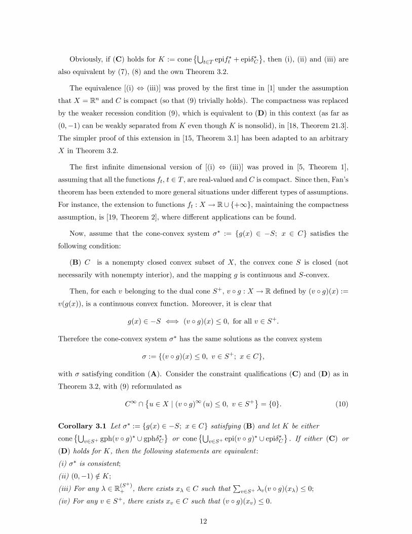
Obviously, if (C) holds for K := cone�S


�C

, then (i), (ii) and (iii) are

also equivalent by (7), (8) and the own Theorem 3.2.

The equivalence [(i) , (iii)] was proved by the �rst time in [1] under the assumption

that X = Rn and C is compact (so that (9) trivially holds). The compactness was replaced

by the weaker recession condition (9), which is equivalent to (D) in this context (as far as

(0;�1) can be weakly separated from K even though K is nonsolid), in [18, Theorem 21.3].

The simpler proof of this extension in [15, Theorem 3.1] has been adapted to an arbitrary

X in Theorem 3.2.

The �rst in�nite dimensional version of [(i) , (iii)] was proved in [5, Theorem 1],

assuming that all the functions ft, t 2 T , are real-valued and C is compact. Since then, Fan�stheorem has been extended to more general situations under di¤erent types of assumptions.

For instance, the extension to functions ft : X ! R[ f+1g, maintaining the compactnessassumption, is [19, Theorem 2], where di¤erent applications can be found.

Now, assume that the cone-convex system �� := fg(x) 2 �S; x 2 Cg satis�es thefollowing condition:

(B) C is a nonempty closed convex subset of X, the convex cone S is closed (not

necessarily with nonempty interior), and the mapping g is continuous and S-convex.

Then, for each v belonging to the dual cone S+, v � g : X ! R de�ned by (v � g)(x) :=v(g(x)), is a continuous convex function. Moreover, it is clear that

g(x) 2 �S () (v � g)(x) � 0; for all v 2 S+:

Therefore the cone-convex system �� has the same solutions as the convex system

� := f(v � g)(x) � 0; v 2 S+; x 2 Cg;

with � satisfying condition (A). Consider the constraint quali�cations (C) and (D) as in

Theorem 3.2, with (9) reformulated as

C1 \�u 2 X j (v � g)1 (u) � 0; v 2 S+

= f0g: (10)

Corollary 3.1 Let �� := fg(x) 2 �S; x 2 Cg satisfying (B) and let K be either

cone�S

v2S+ gph(v � g)� [ gph��Cor cone

�Sv2S+ epi(v � g)� [ epi��C

: If either (C) or

(D) holds for K, then the following statements are equivalent :

(i) �� is consistent;

(ii) (0;�1) =2 K;(iii) For any � 2 R(S

+)+ , there exists x� 2 C such that

Pv2S+ �v(v � g)(x�) � 0;

(iv) For any v 2 S+, there exists xv 2 C such that (v � g)(xv) � 0.

12

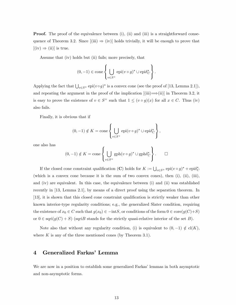
Proof. The proof of the equivalence between (i), (ii) and (iii) is a straightforward conse-

quence of Theorem 3.2. Since [(iii) ) (iv)] holds trivially, it will be enough to prove that

[(iv) ) (ii)] is true.

Assume that (iv) holds but (ii) fails; more precisely, that

(0;�1) 2 cone

8<: [v2S+

epi(v � g)� [ epi��C

9=; :Applying the fact that

Sv2S+ epi(v�g)� is a convex cone (see the proof of [13, Lemma 2.1]),

and repeating the argument in the proof of the implication [(iii)=)(ii)] in Theorem 3.2, it

is easy to prove the existence of v 2 S+ such that 1 � (v � g)(x) for all x 2 C. Thus (iv)also fails.

Finally, it is obvious that if

(0;�1) =2 K = cone

8<: [v2S+


9=; ;one also has

(0;�1) =2 K = cone

8<: [v2S+

gph(v � g)� [ gph��C

9=; : �

If the closed cone constraint quali�cation (C) holds for K :=Sv2S+ epi(v � g)� + epi��C

(which is a convex cone because it is the sum of two convex cones), then (i), (ii), (iii),

and (iv) are equivalent. In this case, the equivalence between (i) and (ii) was established

recently in [13, Lemma 2.1], by means of a direct proof using the separation theorem. In

[13], it is shown that this closed cone constraint quali�cation is strictly weaker than other

known interior-type regularity conditions; e.g., the generalized Slater condition, requiring

the existence of x0 2 C such that g(x0) 2 �intS, or conditions of the form 0 2 core(g(C)+S)or 0 2 sqri(g(C) + S) (sqriB stands for the strictly quasi-relative interior of the set B).

Note also that without any regularity condition, (i) is equivalent to (0;�1) =2 cl(K),where K is any of the three mentioned cones (by Theorem 3.1).

4 Generalized Farkas�Lemma

We are now in a position to establish some generalized Farkas�lemmas in both asymptotic

and non-asymptotic forms.

13

Theorem 4.1 (Asymptotic Farkas� lemma). Let � = fft(x) � 0; t 2 T ;x 2 Cg be aconsistent convex system satisfying condition (A), v 2 X� and � 2 R. Then, the followingstatements are equivalent :

(i) ft(x) � 0 for all t 2 T and x 2 C =) v(x) � �;(ii) (v; �) 2 cl cone

�St2T epif

�t [ epi��C

�.

Proof. Let

�2 :=

8<: ut(x) � f�t (ut) + �; ut 2 domf�t ; t 2 T; � 2 R+u(x) � ��C(u) + �; u 2 dom��C ; � 2 R+

9=; :Recalling that � and �2 have the same solutions, it follows from Lemma 2.4 that (i) is

equivalent to

(v; �) 2 cl cone fB [ (0; 1)g ;

where B denotes the set of coe¢ cient vectors of �2, i.e., B =St2T epif

�t [ epi��C . Since

(0; 1) 2 cl coneB, (i) is in fact equivalent to

(v; �) 2 cl cone

[t2T


!: �

As a consequence of Theorem 4.1, K = cl cone�S


�is the greatest

convex cone K such that fv (x) � �; (v; �) 2 Kg is a linearization of �.

An asymptotic Farkas�lemma similar to Theorem 4.1 can be found in [11, Corollary 2.1],

where the right-hand side of the inclusion in (ii) is expressed in terms of �-subdi¤erentials

of the functions ft, for all t 2 T . The next result was established in [11, Theorem 2.1].

Corollary 4.1 Let � = fft(x) � 0; t 2 T ;x 2 Cg be a consistent convex system satisfying

condition (A) and let f : X ! R [ f+1g be a proper l.s.c. convex function. Then thefollowing statements are equivalent :

(i) ft(x) � 0 for all t 2 T and x 2 C =) f(x) � 0;

(ii) epif� � cl cone�S


�.

Proof. Since fv(x) � �; (v; �) 2 epif�g is a linearization of ff(x) � 0g, (i) is equivalent tothe fact that, for each (v; �) 2 epif�,

ft(x) � 0 for all t 2 T and x 2 C =) v(x) � �:

14

By Theorem 4.1 the last implication is equivalent to

(v; �) 2 cl cone [t2T


!

for each (v; �) 2 epif�t . This is (ii). �

The next straightforward consequence of Corollary 4.1 extends the dual characterization

of set containments of convex sets in [12, Theorem 3.2].

Corollary 4.2 Let fft(x) � 0; t 2 T ;x 2 Cg and fhw(x) � 0; w 2W ;x 2 Dg be consistentconvex systems on X satisfying condition (A), and let A and B be the respective solution

sets. Then, A � B if and only if

[w2W

epih�w [ epi��D � cl cone [t2T


!:

Consequently, A = B if and only if

cl cone

[w2W

epih�w [ epi��D

!= cl cone

[t2T


!:

Now we prove that a nonasymptotic version of Farkas�lemma can be obtained under

both regularity conditions.

Theorem 4.2 (Nonasymptotic Farkas� lemma). Let � = fft(x) � 0; t 2 T ;x 2 Cg be aconsistent convex system satisfying condition (A), v 2 X��f0g; and � 2 R.

If (D) holds for K := cone�S


; then the following statements are

equivalent to each other:

(i) ft(x) � 0; 8t 2 T; and x 2 C =) v(x) � �;

(ii) �(v; �� ) 2 K; 8� > 0;

(iii)

sup�2R(T )+

infx2C

(v(x) +

Xt2T

�tft(x)

)� �: (11)

If (C) holds for K := cone�S


, the following condition can be added

to the list of equivalent statements:

(iv) �(v; �) 2 K:

Moreover, the supremum in (11) is attained, and (iii) can be replaced by

15

(iii�) There exists � 2 R(T )+ such that

v(x) +Xt2T

�tft(x) � �; 8x 2 C: (12)

Remark 4.1 Observe that [(iv) =) (ii)]. In fact, (iv) entails the existence of � 2 R(T )+ ;

ut 2 dom f�t ; �t � 0; for each t 2 T , u 2 dom ��C , and � � 0; such that

�(v; �) =Xt2T

�t(ut; f�t (ut) + �t) + (u; �

�C(u) + �): (13)

Consequently,

�(v; �� ) =Xt2T

�t(ut; f�t (ut) + �t) + (u; �

�C(u) + � + �) 2 K:

Proof. Assume that (D) holds for K := cone�S


.

[(i) =) (ii)] The statement (i) is equivalent to the inconsistency of the system

�(�) :=

8>><>>:ft(x) � 0; t 2 T;v(x)� �+ � � 0;x 2 C

9>>=>>; ;whichever � > 0 we take. Observe that �(�) satis�es (D) for the cone

K + cone epi(v(:)� �+ �)� = K + cone f(v; �� + �) j � � 0g :

The equivalence between (i) and (ii) in Theorem 3.2 entails that �(�) is inconsistent if

and only if

(0;�1) 2 K + cone f(v; �� + �) j � � 0g :

Since � = fft(x) � 0; t 2 T ;x 2 Cg is consistent, Theorem 3.2 precludes (0;�1) 2 K;and there must exist � > 0 and � � 0 such that

(0;�1) 2 K + � (v; �� + �) ;

and so,

�(v; �� ) 2 1�fK + (0; 1 + ��)g � 1

�K = K:

[(ii) =) (iii)] If we apply now the equivalence between (i) and (iii) in Theorem 3.2, �(�)

will be inconsistent, for every � > 0; if and only if there exist �� 2 R(T )+ and �� 0 suchthat

��(v(x)� �+ �) +Xt2T

��t ft(x) > 0; for all x 2 C: (14)

16

It must be �� > 0 (otherwise, the system � = fft(x) � 0; t 2 T ;x 2 Cg will be inconsistent(once again by Theorem 3.2). De�ning p := ��=��, (14) yields

infx2C

(v(x) +

Xt2T

�t ft(x)

)� �� :

Now, letting � # 0 we obtain (11).

[(iii) =) (i)] Now we assume (11). Given � > 0, there exists �� 2 R(T )+ such that

infx2C

(v(x) +

Xt2T

��t ft(x)

)� ��

2:

Then

infx2C

((v(x)� �+ �) +

Xt2T

��t ft(x)

)� �

2> 0;

so that �(�) is inconsistent (again by Theorem 3.2), i.e., (i) holds.

In the second part of the proof, we assume that (C) is satis�ed for the cone K =

cone�S


. Under this assumption, (ii) implies (iv) as far as K is closed,

and so, (ii) and (iv) are equivalent according to the remark previous to the proof.

Now the equivalence of (i) and (iv) follows immediately from Theorem 4.1 and the

closed cone constraint quali�cation (C). It su¢ ces to prove that (iv) implies (iii�) since the

implication [(iii�) =) (iii)] is obvious.

[(iv) =) (iii�)] We have already seen that (iv) entails the existence of � 2 R(T )+ ; ut 2dom f�t ; �t � 0; for each t 2 T , u 2 dom ��C , and � � 0; such that (13) holds, which is

equivalent to

�v =Xt2T

�tut + u; (15)

and

�� =Xt2T

�tf�t (ut) + �

�C(u) +

Xt2T

�t�t + � (16)

�Xt2T

�tf�t (ut) + �

�C(u):

Note that for each x 2 X, ��C(u) � u(x)� �C(x) and f�t (ut) � ut(x)� ft(x), for each t 2 T .It follows from (16) that

�� Xt2T

�t(ut(x)� ft(x)) + u(x)� �C(x):

17

Taking (15) into account, the last inequality implies

�� v(x)�Xt2T

�tft(x)� �C(x)

for all x 2 X. Thus for all x 2 C, we have

v(x) +Xt2T

�tft(x) � �;

which proves (iii�). The proof is complete. �

Observe that, if cone�S


�C

�is closed, then Lemma 2.1 allows us to replace

\ [ " with \ + " in Theorem 4.2.

The next corollary is a straightforward consequence of Theorem 4.2 (see also Corollary

3.1).

Corollary 4.3 Let �� := fg(x) 2 �S; x 2 Cg satisfying (B) and let u 2 X�, � 2 R. Ifcone(

Sv2S+ epi(v�g)�[epi��C) is weak�-closed, then the following statements are equivalent

to each other :

(i) g(x) 2 �S and x 2 C =) u(x) � �;(ii) �(u; �) 2 cone(

Sv2S+ epi(v � g)� [ epi��C);

(iii) There exists v 2 S+ such that u(x) + (v � g)(x) � �; for all x 2 C:

5 Optimality Conditions for Convex Programs

Let � = fft(x) � 0; t 2 T ;x 2 Cg be a consistent convex system satisfying condition (A).

Consider the convex optimization problem

(CP) Minimize f(x)

subject to ft(x) � 0; t 2 T;

x 2 C;

where f is a proper l.s.c. convex funtion.

Let A := fx 2 C j ft(x) � 0; t 2 Tg be the feasible set of (CP), and assume thatA \ domf 6= ;:

A �rst question to be addressed is the existence of points in A minimizing the value of

the objective function. These points are called minimizers of the problem (CP).

18

Proposition 5.1 If X is the Euclidean space and (9) holds, the set of minimizers of (CP)

is non-empty.

Proof. The function

h := f + �A

is a proper l.s.c. convex function (as a consequence of the fact that A \ domf 6= ;) suchthat

fz 2 X j h1(z) � 0g = fz 2 X j f1(z) � 0g \A1 = f0g;

since, according with [18, Theorem 9.4],

A1 = C1 \ fz 2 X j f1t (z) � 0; t 2 Tg = f0g:

By [18, Theorem 27.2] h attains its in�mum at points which are, obviously, minimizers of

(CP). �

Remark 5.1 The statement in Proposition 5.1 can be false even in the case that X is a

re�exive Banach space, as the following example shows:

Example 5.1 Let us consider the convex optimization problem in the Hilbert space `2

(CP) Minimize ff(x) j x 2 Cg;

where x = (�n)n�1 2 `2;

C :=�x 2 `2 jj�nj � n; 8n 2 N

;

and

f(x) :=1Xn=1

�nn:

If a := (�n)n�1 with �n = 1=n; n = 1; 2; :::; we have a 2 `2 and f is a continuous linear(and, so, convex) functional on `2:

In [21, Example 1.1.1] it is proved that C is a closed convex set which is not bounded

(because nen 2 C; for every n 2 N) and such that C1 = f0g: Therefore, the recessioncondition (9) trivially holds. Moreover if we de�ne ck := ( kn)n�1; k = 1; 2; :::;

kn :=

8<: �n; if n � k;0; if n > k;

it is also evident that ck 2 C; for all k 2 N; and f(ck) = �k: Thus, we conclude that f isnot bounded from below on C and no minimizer exists.

19

[21, Exercise 2.41] provides di¤erent characterizations of the coerciveness of a proper

l.s.c. convex function de�ned on a normed space, but none of them directly involves the

notion of recession direction. Theorem 2.5.1 in [21] establishes that if X is a re�exive

Banach space and the function f + �A is coercive, then the set of minimizers is non-empty.

Theorem 5.1 Suppose that the set epif� + epi��A is weak�-closed. Then a 2 A is a mini-

mizer of (CP) if and only if there exists v 2 @f(a) such that

�(v; v(a)) 2 cl cone [t2T


!:

Proof. Since (CP) can be written as infff(x) j x 2 Ag, we have that a 2 A is a minimizerif and only if

0 2 @(f + �A)(a):

Since epif�t + epi��A is weak

�-closed, by Lemma 2.2 the last inclusion is equivalent to

0 2 @f(a) +NA(a):

In fact this condition is also equivalent to the existence of v 2 @f(a) such that v(x) � v(a)for each x 2 A; i.e., there exists v 2 @f(a) such that

ft(x) � 0; 8t 2 T; and x 2 C =) v(x) � v(a):

By Theorem 4.1, the last implication is equivalent to

�(v; v(a)) 2 cl cone [t2T


!:

The theorem is proved. �

Theorem 5.2 Suppose that epif� + epi��A and cone�S


�are weak�-closed

sets. Then a 2 A is a minimizer of (CP) if and only if there exist v 2 @f(a) and � 2 R(T )+

such that

�v 2 @(Xt2T

�tft + �C)(a) (17)

and

�tft(a) = 0; 8t 2 T: (18)

Moreover, if the functions ft; t 2 T , are continuous at a then (17) can be replaced by

0 2 @f(a) +Xt2T

�t@ft(a) +NC(a):

20

Proof. It follows from Theorem 5.1 that a 2 A is a minimizer of (CP) if and only if thereexist v 2 @f(a) such that

�(v; v(a)) 2 cone [t2T


!: (19)

(Note that the cone in the right-hand side of (19) is weak�-closed by the assumption.)

By Theorem 4.2, (19) is equivalent to the existence of � 2 R(T )+ satisfying

v(x) +Xt2T

�tft(x) � v(a); 8x 2 C:

Taking x = a in the last inequality, we get �tft(a) = 0 8t 2 T . It is also clear that a is aminimizer of the problem

(P1) infx2C

(v(x) +

Xt2T

�tft(x)

);

which implies that

0 2 @(v +Xt2T

�tft + �C)(a);

or equivalently,

�v 2 @(Xt2T

�tft + �C)(a):

The necessity is proved.

Conversely, if (17) is satis�ed then a is a solution of Problem (P1) and hence,

v(x) +Xt2T

�tft(x) � v(a) +Xt2T

�tft(a); 8x 2 C:

Due to (18) one actually has

v(x) +Xt2T

�tft(x) � v(a); 8x 2 C:

Now if x 2 C and ft(x) � 0; 8t 2 T; then v(x) � v(a). This means that v(x) � v(a) for

all x 2 A. This is, in turn, equivalent to 0 2 @f(a) + NA(a), which implies that a is aminimizer of (CP).

Moreover, if all the functions ft, t 2 T; are continuous at a then

@(Xt2T

�tft + �C)(a) =Xt2T

�t@ft(a) +NC(a):

(See, for instance, [16, Theorem 5.3.32]). In this way, the last assertion of the theorem

follows. �

21

Remark 5.2 The set epif� + epi��A is weak�-closed when f is linear. In fact, epif� is a

vertical hal�ine (locally compact, as far it is �nite-dimensional), ��A is proper and so,

(�epif�)1 \ (epi��A)1 = f0g:

Then the Dieudonné theorem applies ([21, Theorem 1.1.8]).

Even in the simple linear case, the assumptions of Theorem 5.2 do not entail the exis-

tence of minimizers. This fact is illustrated in the following example.

Example 5.2 Consider the linear optimization problem, in R2;

(CP) Minimize x1

subject to � 1tx1 + x2 � log(t)� 1; t 2]0; 1];

x1 � 0 and x2 � 0:

Let f(x) = x1, ft(x) = �1tx1 + x2 � log(t) + 1, t 2]0; 1], f0(x) = �x1, and f2(x) =

x2; with x = (x1; x2) 2 R2. Let also T = ]0; 1] [ f0; 2g. Note that in this case, C =

R2 and all the constraints are linear inequalities. In [7, Exercise 8.8] it is stated that

cone�S

t2T epif�t [ epi��Rn

�is weak�-closed. It follows from Remark 5.2 that epi f�+epi ��A

is also a weak�-closed set. However, the set of minimizers is empty.

We consider �nally the cone-convex problem

(CCP) Minimize f(x)

subject to g(x) 2 �S;

x 2 C;

where the constraint system �� satis�es condition (B). The following optimality condition

for (CCP) was established in [3, Theorem 4.1] (see also [13]) for the case where X and Y

are Banach spaces and under the conditions that the setsSv2S+ epi(v � g)� + epi��C and

epif�+Sv2S+ epi(v�g)�+epi��C are weak�-closed. The next result relaxes these conditions.

Corollary 5.1 Suppose that cone�S

v2S+ epi(v � g)� [ epi��C�and

epif� + cone(Sv2S+ epi(v � g)� [ epi��C) are weak�-closed. Then a 2 A is a minimizer of

(CCP) if and only if there exist v 2 @f(a) and v 2 S+ such that

0 2 @f(a) + @(v � g)(a) +NC(a) and (v � g)(a) = 0:

22

Proof. Note that the constraint g(x) 2 �S is equivalent to gv(x) := (v � g)(x) � 0 for allv 2 S+. Moreover, by the assumption on the map g, for each v 2 S+, gv is continuous. Onthe other hand, by [13, Lemma 2.1], we have

epi��A = cl

0@ [v2S+

epi(v � g)� + epi��C

1A :It follows from Lemma 2.1 and the assumptions of the corollary that

epi��A = cone

0@ [v2S+


1A :The conclusion follows by the same argument as in the proof of Theorem 5.2, using Corollary

4.3 instead of Theorem 4.2. �

References

[1] F. Bohnenblust, S. Karlin and L. S. Shapley, Games with continuous pay-o¤, Annals

of Mathematics Studies, 24 (1950), 181-192.

[2] J.M. Borwein, The limiting Lagrangian as a consequence of Helly�s theorem, Journal

of Optimization Theory and Applications, 33 (1981), 497-513.

[3] R.S. Burachik and V. Jeyakumar, Dual condition for the convex subdi¤erential sum

formula with applications, Journal of Global Analysis, to appear.

[4] Yung-Chin Chu, Generalization of some fundamental theorems on linear inequalities,

Acta Mathematica Sinica, 16 (1966), 25-40.

[5] K. Fan, Existence theorems and extreme solutions for inequailities concerning convex

functions or linear transformations, Mathematische Zeitschrift, 68 (1957), 205-217.

[6] M. A. Goberna, V. Jeyakumar, and N. Dinh, Dual characterizations of set containments

with strict convex inequalities, Journal of Global Optimization, to appear.

[7] M. A. Goberna and M. A. López, Linear Semi-in�nite Optimization, Wiley Series in

Mathematical Methods in Practice, John Wiley & Sons, Chichester, 1998.

[8] M. A. Goberna, M. A. López, J. A. Mira, and J. Valls, On the existence of solutions

for linear inequality systems, Journal of Mathematical Analysis and Applications, 192

(1995), 133-150.

23

[9] Ch.-W Ha, On systems of convex inequalities, Journal of Mathematical Analysis and

Applications, 68 (1979), 25-34.

[10] R. B. Holmes, Geometric Functional Analysis, Springer-Verlag, Berlin, Germany, 1975.

[11] V. Jeyakumar, Asymptotic dual conditions characterizing optimality for in�nite convex

programs, Journal of Optimization Theory and Applications, 93 (1997), 153-165.

[12] V. Jeyakumar, Characterizing set containments involving in�nite convex constraints

and reverse-convex constraints, SIAM J. Optimization, 13 (2003), 947-959.

[13] V. Jeyakumar, N. Dinh, and G. M. Lee, A new closed cone constraint quali�cation

for convex Optimization, Applied Mathematics Research Report AMR04/8, UNSW,

2004. See

http://www.maths.unsw.edu.au/applied/reports/amr08.html

[14] V. Jeyakumar, A. M. Rubinov, B. M. Glover and Y. Ishizuka, Inequality systems and

global optimization, Journal of Mathematical Analysis and Applications, 202 (1996),

900-919.

[15] M. A. López and E. Vercher, Convex semi-in�nite games, Journal of Optimization

Theory and Applications, 50 (1986), 289-312.

[16] Z. Denkowski, S. Migórski and N.S. Papageorgiou, An Introduction to Nonlinear Analy-

sis. Theory, Kluwer Academic Publishers, Boston, 2003.

[17] R. T. Rockafellar, Level sets and continuity of conjugate convex functions, Transactions

of the American Mathematical Society, 123 (1966), 46-63.

[18] R. T. Rockafellar, Convex Analysis, Princeton Univ. Press, Princeton, N. J., 1970.

[19] N. Shioji and W. Takahashi, Fan�s theorem concerning systems of convex inequalities

and its applications, Journal of Mathematical Analysis and Applications, 135 (1988),

383-398.

[20] Jan van Tiel, Convex Analysis, John Wiley and Sons, Belfast, 1984.

[21] C. Z¼alinescu, Convex Analysis in General Vector Spaces, World Scienti�c, New Jersey,

2002.

24

from linear to convex systems: consistency, farkas™ lemma

Documents