freshwater accounting: draft guidance for regional … water...2.2 why do we need to account for...
TRANSCRIPT

Freshwater Accounting: Draft Guidance for Regional Authorities

Disclaimer
The opinions and options contained in this document are for general guidance purposes only. Please seek specific legal advice from a qualified professional person before undertaking any action based on the contents of this publication. The contents of this document must not be construed as legal advice. The Crown does not accept any responsibility or liability whatsoever to any person for an action taken as a result of reading, or reliance placed because of having read any part, or all, of the information in this document, or for any error, inadequacy, deficiency, flaw in or omission from this document.
Acknowledgements
We would like to extend sincere thanks to all of those who provided input to the development of this guidance, including:
The NIWA-led project team that prepared the original report, which formed the basis of the content of this guidance: Helen Rouse (NIWA), Jim Cooke (Streamlined Environmental Ltd), and Channa Rajanayaka (Aqualinc). Also, thanks to the reviewers of this report: Clive Howard-Williams, Sandy Elliot and Graeme Horrell (NIWA), and John Bright (Aqualinc).
All council representatives who participated in workshops, provided case studies, and reviewed early drafts: Ken Taylor, Dennis Jamieson (Environment Canterbury), Melissa Robson (Environment Canterbury and AgResearch), Matt Hickey (Otago Regional Council), Kirsteen MacDonald (Auckland Council), Jon Roygard (Horizons Regional Council), Bill Vant (Waikato Regional Council), and Mary-Anne Baker and Steve Markham (Tasman District Council).
The Land and Water Forum for providing feedback on the original input report.
This report may be cited as:
Ministry for the Environment. 2014. Freshwater Accounting: Guidance for Regional Authorities. Wellington: Ministry for the Environment
Published in December 2014 by the Ministry for the Environment Manatū Mō Te Taiao PO Box 10362, Wellington 6143, New Zealand
ISBN: 978-0-478-41261-1
Publication number: ME 1171
© Crown copyright New Zealand 2014
This document is available on the Ministry for the Environment’s website: www.mfe.govt.nz
Freshwater Accounting: Draft Guidance for Regional Authorities 3
Contents
1 Introduction 5
1.1 Document structure 5
1.2 Development of this guidance 6
2 Background 7
2.1 What is freshwater accounting? 7
2.2 Why do we need to account for fresh water? 7
2.3 Relationship with other freshwater management instruments 8
3 Principles of freshwater accounting 11
4 General advice 13
4.1 The importance of scale and significance 13
4.2 Setting freshwater management units (FMUs) 15
4.3 Spatial resolution of accounting 18
4.4 Frequency of accounting 21
4.5 The need for flexibility 24
4.6 Comments on using models 26
4.7 Estimating accuracy and uncertainties 28
4.8 Presenting information to your communities 30
5 Key components of accounting systems 32
5.1 The key components of accounting 32
5.2 Water quantity 33
5.3 Water quality 46
References 69
4 Freshwater Accounting: Draft Guidance for Regional Authorities
Figures
Figure 2.1: Year-to-year variations in the components of the national water accounts, 1995–2010 9
Figure 2.2: Estimated annual water use by regions 10
Figure 4.1: Using resource pressure and other influences in a risk-based approach to selecting the size of WMZs in the Horizons region 15
Figure 4.2: Map of Canterbury's 10 water management zones (WMZ) 17
Figure 4.3: Allocated versus used surface water volumes in the Canterbury region (2011–2012 water year) 19
Figure 4.4: The allocated and actual daily use in a part of Waihou catchment, March 2013 20
Figure 4.5: Percentage contribution from different land uses to nitrogen load in upper Manawatu River 21
Figure 4.6: Returns received and actual weekly use for the Moutere Eastern Groundwater Zone, November 2012 to May 2013 23
Figure 4.7: The allocated and actual daily use on the two days preceding 21 June 2013, for the Ohau catchment 24
Figure 4.8: Snapshot of water quality data for the Ashburton catchment, from the LAWA website 31
Figure 5.1: Key components of freshwater accounting for water quantity and quality 32
Figure 5.2: Screenshot from Water Matters from the Rangitikei catchment, July 2014 39
Figure 5.3: Screenshot of the rate of take and monthly volume used for a water take in the Kakanui River 40
Figure 5.4: Horizons Regional Council’s water quantity accounting system 43
Figure 5.5: Auckland Council’s water quantity accounting system 43
Figure 5.6: Waikato Regional Council’s water quantity accounting system 44
Figure 5.7: Schematic summary of zinc sediment quality guideline exceedance in the Central Waitemata Harbour based on modeling zinc inputs from the catchment 48
Figure 5.8: Classification of catchment scale water quality models in New Zealand 54
Figure 5.9: An example of output from URQIS for ammoniacal-N summarised by region 61
Figure 5.10: Predicting TN concentrations in the Pueto catchment using three different attenuation factors 65
Tables
Table 3.1: Principles of freshwater accounting 11
Table 4.1: Key water use and allocation statistics for Auckland Region 19
Table 5.1: A suggested template for water quantity accounting 45
Table 5.2: Attributes to be managed under the National Objectives Framework 46
Table 5.3: Mass flows of nitrogen and phosphorus in the Waikato River catchment during 2003–2012 58
Table 5.4 Catchment target and limits for nitrogen losses from farming activities, community sewerage systems, and industrial or trade processes 60
Table 5.5: A suggested template for water quality accounting (per contaminant) 68

Freshwater Accounting: Draft Guidance for Regional Authorities 5
1 Introduction
The National Policy Statement for Freshwater Management (NPS-FM)1 requires that regional
councils and unitary authorities establish freshwater accounting systems for both water
quantity and quality. This document provides guidance on how to establish freshwater
accounting systems to meet the requirements of the NPS-FM. Its primary audience is people
working in regional councils and unitary authorities (hereafter referred to as ‘councils’).
However, other stakeholders, such as those involved in collaborative decision-making
processes with councils, may also find it of value.
This guide is published as a draft to enable councils and other practitioners to provide
feedback to the Ministry before it is finalised.
1.1 Document structure
There is no single correct or preferred way to establish a freshwater accounting system to
meet the requirements of the NPS-FM. Instead, each system needs to reflect the issues of the
fresh water for which the accounts are being generated. Therefore, to allow councils flexibility
to establish a freshwater accounting system that suits their unique needs, the Ministry for
the Environment has avoided providing prescriptive guidance on ‘how to account for fresh
water’. Instead, this document provides advice on the principles and key components that
make up a successful accounting system, along with general advice and explanations. Case
studies are used to illustrate key points raised in the text and/or show how the concepts may
work in practice.
The outline of the remainder of this document is as follows:
Section 2 – explains what freshwater accounting is, and the relationship between the NPS-FM
accounting requirement and other instruments used to manage fresh water.
Section 3 – outlines nine principles for freshwater accounting that encapsulate the
fundamentals of good accounting practice.
Section 4 – provides general advice on matters such as the importance of scale and
significance, spatial and temporal resolution of accounting, using models, and dealing with
uncertainties.
Section 5 – outlines the key components of accounting and the main steps involved in
establishing accounting systems for both water quantity and water quality.
A high level overview of the NPS-FM, including the freshwater accounting guidance
requirements, is in the National Policy Statement for Freshwater Management 2014: Draft
Implementation Guide.2 This provides background and context information, as well as policy
1 http://www.mfe.govt.nz/publications/fresh-water/national-policy-statement-freshwater-management-2014.
2 http://www.mfe.govt.nz/publications/fresh-water/national-policy-statement-freshwater-management-2014-
draft-implementation.

6 Freshwater Accounting: Draft Guidance for Regional Authorities
interpretation of the NPS-FM. Also, the glossary in the Draft Implementation Guide explains
the terminology used in this guidance.
1.2 Development of this guidance
In 2014, the Ministry for the Environment engaged a project team lead by the National
Institute of Water and Atmospheric Research (NIWA) to help develop freshwater accounting
guidance. The team’s report forms the basis of this guidance.
Staff from six councils were also involved and provided valuable input throughout its
development.
All contributors are listed in the Acknowledgements on the inside cover of this document.

Freshwater Accounting: Draft Guidance for Regional Authorities 7
2 Background
This section explains what freshwater accounting is, and the relationship between the NPS-FM
accounting requirement and other freshwater management instruments.
2.1 What is freshwater accounting?
The term ‘freshwater accounting’ refers to collecting information about the existing water use
and the pressures of the freshwater resources being managed. To do this, freshwater
accounting must be carried out for both water quality and quantity.
The NPS-FM defines freshwater accounting systems as the following:
“Freshwater quality accounting system” means a system that, for each freshwater
management unit, records, aggregates and keeps regularly updated, information on the
measured, modelled or estimated:
a) loads and/or concentrations of relevant contaminants;
b) sources of relevant contaminants;
c) amount of each contaminant attributable to each source; and
d) where limits have been set, proportion of the limit that is being used.
“Freshwater quantity accounting system” means a system that, for each freshwater
management unit, records, aggregates and keeps regularly updated, information on the
measured, modelled or estimated:
a) total freshwater take;
b) proportion of freshwater taken by each major category of use; and
c) where limits have been set, the proportion of the limit that has been taken.
Within a freshwater quantity accounting system, all water taken from the water body must be
quantified. This includes water taken under resource consent (both the total amount allocated
within the consent and the amount of water that is actually taken), as well as any takes that
are permitted or do not require a resource consent, such as stock water.
Similarly, a freshwater quality accounting system requires all relevant contaminants that are
being discharged to fresh water to be quantified. This includes both point sources and diffuse
sources of contaminants.
2.2 Why do we need to account for fresh water?
It is essential to have good information on how we use fresh water to make effective decisions
on objectives for and limits on that use, as well as managing within them. Freshwater
accounting is one part of this information. The NPS-FM requires councils to establish
freshwater accounting systems (Part CC) in freshwater management units (FMU) where
decisions on freshwater management practices are being made. The aim is to deliver an
improved ability to set freshwater objectives and limits at regional level.

8 Freshwater Accounting: Draft Guidance for Regional Authorities
The four main reasons we need to account for fresh water are to:
inform decisions on the setting and reviewing of objectives and limits
inform decisions on how to manage within limits, once set, to determine where reductions
in discharges are needed, or where quantity is over-allocated
provide feedback to communities on progress against set objectives and act as a trigger
for any needed changes in management practices
provide information for investors about catchments where there are freshwater resources
available and where constraints exist for further development.
2.3 Relationship with other freshwater management instruments
While this guide covers the need for accounting as required by the NPS-FM , it is important
that councils are aware of other developments that may result in more prescriptive future
requirements to collate regional records and report at the national level.
The Draft Implementation Guide provides a summary of how the NPS-FM relates to national
environmental standards (NES), national policy statements (NPS), the Resource Management
(Measurement and Reporting of Water Takes) Regulations 2010, water conservation orders
(WCO), the Environmental Reporting Bill, the Resource Management Act 1991 (RMA), Treaty
settlement legislation, and the Hauraki Gulf Marine Park Act 2000.
Of particular relevance to freshwater accounting are the Resource Management
(Measurement and Reporting of Water Takes) Regulations 2010 (commonly referred to as
the ‘water metering regulations’) and the Environmental Reporting Bill.
The water metering regulations require consent holders of water takes greater than five litres
per second to collect records of their water use and provide annual records to their council3
(unless the use of the water is non-consumptive, as set out in regulation 4(2)). The information
generated under these regulations will be a substantial component of freshwater accounting,
particularly for quantity. The regulations include staged implementation of reporting based on
take size. Work is currently in progress to collate this information at the national level in a way
that ensures it is comparable between regions.
The Environmental Reporting Bill aims to create a national-level reporting system covering five
environmental domains, of which fresh water is one. If enacted, it will result in the production
of a report for one of the five domains every six months, and a synthesis report every three
years.4 The freshwater domain report will include information on the biophysical state of the
freshwater domain, trends over time, pressures driving changes in the state, and the impacts
of changes in the state on ecosystem integrity, public health, economic benefits, and culture
and recreation.
To help deliver these reports, work has been under way for several years to look at
Environmental Monitoring and Reporting (EMaR) protocols, methods, and data management.
As a result there will be some additional requirements for councils, mainly to ensure statistical
3 http://www.mfe.govt.nz/fresh-water/regulations-measurement-and-reporting-water-takes.
4 http://www.mfe.govt.nz/more/environmental-reporting/about-environmental-reporting-nz/our-
environmental-reporting-programme.

Freshwater Accounting: Draft Guidance for Regional Authorities 9
rigour. The council-led EMaR development group intends that national reporting of the state
and pressures on fresh water will be aggregated firstly at the regional level (from FMUs) and
then at the national level. However, indicators for state of the environment (SoE) reporting
have not yet been finalised. Further information will be developed on how to provide data
for EMaR.
Case studies 2.1 and 2.2 describe previous national level projects to collate and analyse water
quantity accounting information.
CASE STUDY 2.1 – NEW ZEALAND WATER PHYSICAL STOCK ACCOUNTS
New Zealand has produced water accounts at a national level, including regional
breakdowns. In 2011, Statistics New Zealand issued the latest report in its
Environmental Accounts series, Water Physical Stock Account: 1995–2010. This report
describes how stocks of fresh water are affected by water flows within the
hydrological system during accounting periods. The account is structured in line with
the System of Environmental – Economic Accounting for Water (United Nations,
2007). The New Zealand water physical stock account is presented in terms of inflows,
outflows, and changes in storage levels.
Figure 2.1 illustrates the variations in components of the surface water system for
each year from 1995 to 2010.
Figure 2.1: Year-to-year variations in the components of the national water accounts, 1995–2010
Source: Statistics New Zealand, 2011, from Henderson et al, 2011.
For more details, see:
http://www.stats.govt.nz/browse_for_stats/environment/environmental-economic-
accounts/water-physical-stock-account-1995-2010.aspx.
-
200,000
400,000
600,000
800,000
1,000,000
1,200,000
1,400,000
1,600,000
1,800,000
2,000,000
1995 1996 1997 1998 1999 2000 2001 2002 2003 2004 2005 2006 2007 2008 2009 2010
Vo
lum
e (
millio
ns o
f m
3/y
ear)
Precipitation Inflow from other regions Evapotranspiration
Abstraction for Hydrogeneration Discharge by Hydrogeneration Outflow to sea
Outflow to other regions Change in Lakes Change in Soil Moisture
Change in Ice Change in Snow

10 Freshwater Accounting: Draft Guidance for Regional Authorities
CASE STUDY 2.2 – WATER ALLOCATION SNAPSHOT
As part of its existing national environmental reporting programme, the Ministry for
the Environment has in the past commissioned several reports to help measure a
national water quantity indicator: the volume of water allocated (via resource
consent) to consumptive uses. (See http://www.mfe.govt.nz/environmental-
reporting/fresh-water/freshwater-demand-indicator/freshwater-demand-
allocation.html).
The most recent report (Aqualinc, 2010) presents a summary of the approach and
results of the 2010 survey of freshwater take consents for both consumptive and non-
consumptive uses, and also includes estimates of actual abstraction volumes of the
consented takes.
Figure 2.2 shows that for most regions (with the exception of Gisborne), water use is
likely well below (65 per cent of) allocation levels. Freshwater accounting information
will help councils understand these differences between allocation and use, and
identify potential situations where paper allocations can be reduced to match actual
use, as well as situations when that may not be desirable. For example, a certain
industrial use (such as frost spraying in horticulture) may often not use its allocation
but still needs that potential water for use.
Figure 2.2: Estimated annual water use by regions
Source: Aqualinc, 2010.
The report is available at: http://www.mfe.govt.nz/publications/rma-fresh-
water/update-water-allocation-data-and-estimate-actual-water-use-consented-3.

Freshwater Accounting: Draft Guidance for Regional Authorities 11
3 Principles of freshwater accounting
To ensure a level of consistency in the approach to freshwater accounting, this section outlines
nine high-level principles of freshwater accounting that encapsulate the fundamentals of
accounting practice. The principles reflect a general philosophy of how freshwater accounting
should ideally contribute to councils’ freshwater management ‘toolbox’.
The nine principles are based on:
the six criteria used to evaluate accounting systems in the stocktake reported in Rouse
et al, 2013
general features outlined in the Australian Standard for water accounting (see:
http://www.bom.gov.au/water/standards/wasb/wasbawas.shtml)
principles and protocols for Tier 1 statistics (see: http://www.mfe.govt.nz/environmental-
reporting/about-environmental-reporting/national-environmental-
indicators/environmental-indicator-criteria/index.html)
principles suggested by council representatives.
Table 3.1: Principles of freshwater accounting
Principles Descriptors
Risk-based Accounting systems should allow for accounts to be generated using methods appropriate to the scale and significance of issues in a FMU.
Identification of relevant contaminant sources should be linked to risks faced in an FMU.
Transparent The purpose of the accounting system should be clearly stated.
Accounting information should be easily accessible by both water users and other stakeholders.
All methods used for accounting should be clearly documented so that calculations are repeatable.
Technically robust Accounting systems should use good practice methods based on relevant science.
Accounting systems should allow comparison between years (or reporting periods) and with other FMUs.
Any errors and uncertainties of methods used should be clearly documented.
Quality assurance steps should be documented, and methods for handling any data issues that may come to light outlined.
Practical Accounting systems should allow for councils to collate information from various existing systems or models (eg, consents databases, monitoring databases).
The systems should allow reports to be generated and displayed for water users and stakeholders.
Accounting systems should be future-proofed, so they are practical over time.

12 Freshwater Accounting: Draft Guidance for Regional Authorities
Principles Descriptors
Effective and relevant
Accounting systems should be fit for purpose – that is, they should allow for the four potential uses of accounting information for regional freshwater management.
Accounting systems should produce meaningful information (accurate, appropriate to the spatial scale of the issues, and useful to the intended end users), noting that this may vary with the purpose of the accounts being produced.
Accounting systems should be cost-effective.
Timely Accounting systems should allow a council to produce regular accounts for water quantity and water quality, and in a suitable form, for the FMUs where freshwater objectives and limits are being set or reviewed.
Accounting systems should allow councils to collect and analyse information at frequencies that are relevant to the intended management use (eg, seasonally, to be relevant to ecological systems and variability in flows; daily, if data will be used for operational water take/restriction management).
Partnership Accounting systems should be developed and information collected in partnership with stakeholders and the community. This will help ensure that water users and stakeholders will accept and use the accounting information produced.
Adaptable Accounting systems should allow for flexibility to accommodate different methods appropriate to the scale and significance of the issues in different FMUs.
The systems should allow for improvements in methods and the accuracy of measurements, estimates, and/or modelling results over time.
Accounting systems should allow for the integrated and iterative nature of freshwater management.
Systems should allow for reporting that is scalable from FMUs (or water management zones, if this is different) to regional level.
Integrated Where appropriate for an FMU, the system should allow for the integration of, for example, surface water and groundwater or discharges to different receiving waters, such as estuaries.

Freshwater Accounting: Draft Guidance for Regional Authorities 13
4 General advice
This section provides general advice on applying the principles in table 3.1. A box at the
beginning of each topic highlights which principle(s) are relevant.
4.1 The importance of scale and significance
The following advice is aligned with two principles: Risk-based, Practical.
While in global terms New Zealand has abundant water (Statistics New Zealand, 2010), our
island weather and topography mean this water is unevenly distributed (Salinger et al, 2004).
Equally, our landscape has varying geology, soils, land use and urban development. Added to
this spatial variability is temporal variability in weather and climate. The relationship between
water use and water quality adds further complexity. While there is an abundance of water as
a whole, there may be high demand (and thus potential scarcity) for suitable water for
particular uses (such as, drinking, recreation, and stock water). The resulting variability in
water supply, demand, runoff, discharges and receiving environments means each region has
very specific water quantity and quality issues to manage.
The NPS-FM, through Policy CC1(b), expects that accounting happens, “at levels of detail that
are commensurate with the significance of the freshwater quality and freshwater quantity
issues, respectively, in each freshwater management unit”. This policy direction is a
fundamental starting point for much of the guidance that follows – that is, that freshwater
management units (or catchments, aquifers, regions, or parts thereof) do not all have the
same water resource management needs. Methods for accounting for all water takes and
all relevant sources of contaminants can therefore vary between freshwater management
units (FMUs).
One way to decide which methods may be appropriate to use is a risk-management approach.
Understanding risk normally requires an understanding of the likelihood and consequences of
an event or action. Freshwater management under the RMA is implicitly risk-based (Rouse and
Norton, 2010).

14 Freshwater Accounting: Draft Guidance for Regional Authorities
CASE STUDY 4.1 – USING A RISK-BASED APPROACH TO SELECT TECHNICAL METHODS
The Draft Guidelines for the Selection of Methods to Determine Ecological Flows (Beca,
2008) outline a risk-based approach for selecting methods to be used to set minimum
flows to protect ecological instream values (as part of setting environmental flows or
limits in NPS-FM terminology).
The system looks at the degree of hydrological alteration (how much water is to be
taken from the water body) to help assess the likelihood aspect of risk, and ranks this
against the significance of values identified for that water body to better understand
the consequence aspect of risk. For example, for rivers, a low degree of alteration and
low significance of values would mean that a simple method (or estimate) could be
used to assess potential ecological flow requirements, such as a hydrological statistic
or expert panel. At the opposite end of the spectrum, a high degree of alteration and
high instream values would suggest a need to use detailed knowledge and models to
predict ecological flow requirements.
See: http://www.mfe.govt.nz/publications/fresh-water/draft-guidelines-selection-
methods-determine-ecological-flows-and-water-24.
A risk-based approach similar to case study 4.1 could be used to select methods for freshwater
accounting, using an understanding of the pressures on water quantity and quality in an FMU
on one hand, and the values of that FMU to its community on the other. A scoping exercise
could help determine priority or high-risk FMUs. For example, the Draft Implementation Guide
suggests that for water quality accounting, a preliminary assessment of likely values and
objectives could be carried out, along with an initial low cost accounting process for the
contaminant(s) most likely to be relevant. Once the possible range of objectives is narrowed,
more accurate accounting may be needed. This is likely in cases where, for example, significant
reductions in discharges of relevant contaminants are needed to achieve some of the
objectives being considered.
This risk-based approach is discussed further in 4.5.

Freshwater Accounting: Draft Guidance for Regional Authorities 15
CASE STUDY 4.2 – HORIZONS REGIONAL COUNCIL’S RISK-BASED SETTING OF FRESHWATER MANAGEMENT UNITS
Horizons Regional Council used a risk-based approach to set its water management
zones (WMZ). In the Whanganui catchment, where the pressures on water are
relatively low, Horizons selected relatively large WMZs. In contrast, for the Manawatu
catchment, where pressures are high, much smaller WMZs were set, enabling more
detailed information to be collected. Figure 4.1 illustrates the criteria used to select
WMZ size.
Figure 4.1: Using resource pressure and other influences in a risk-based approach to selecting the size of WMZs in the Horizons region
More can be found at:
http://www.horizons.govt.nz/assets/horizons/Images/Development%20of%20Water%2
0Management%20Zones%20in%20the%20MW%20Reg.pdf.
4.2 Setting freshwater management units (FMUs)
The following advice is aligned with four principles: Technically robust, Effective and relevant,
Adaptable, Integrated.
FMUs are the fundamental units of a freshwater quantity and quality accounting system. They
represent the area within which common freshwater objectives and limits are set. The NPS-FM
defines a freshwater management unit as, “the water body, multiple water bodies or part of a
water body determined by the regional council as the appropriate spatial scale for setting

16 Freshwater Accounting: Draft Guidance for Regional Authorities
freshwater objectives and limits and for freshwater accounting and management purposes”.
Accounts for FMUs will enable comparisons between them, aggregation to explore regional
issues, and potentially further aggregation to a national level (although this is not currently a
requirement). A monitoring plan is required to provide representative data appropriate to the
pressures and state of the FMU in question (Part CB of the NPS-FM).
Further guidance on setting FMUs will be provided by the Ministry for the Environment in
2015. However, the main point to note is that the number and scale of FMUs in a region is
critical. FMUs should reflect common objectives for the waterbody or bodies within it, so that
representative monitoring sites can be readily established. This means FMUs should be not just
hydrologically coherent, but also socially, so that communities and iwi with common interests
and values are contributing to common objectives.
Many councils had already set water management zones or units before the introduction of
the NPS-FM – such zones may or may not be the same as an FMU. For instance, they may need
scaling up or down for particular issues being addressed, to contribute to a common objective
being set for an FMU. These zones may have been set for water quantity management
purposes and may need to be reviewed to assess whether they are also appropriately scaled
for water quality management issues.
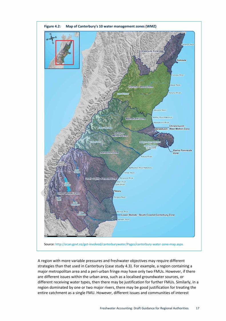
CASE STUDY 4.3 – SETTING WATER MANAGEMENT ZONES IN CANTERBURY
The Water Management Zones (WMZs) chosen by Environment Canterbury (figure 4.2)
are an example of FMUs intended to reflect common interest and management
objectives.
They were developed before the NPS-FM requirement for FMUs to be set. The WMZs
were designed to enable implementation of the Canterbury Water Management
Strategy where the main issue was sustainable irrigation development. They have since
been incorporated into the Canterbury Land and Water Plan.
In some cases the WMZ incorporates a whole catchment (eg, Ashburton), although
where collaborative limit-setting processes are being undertaken, these have been
divided into smaller units (such as the Hinds catchment). Other WMZs include only part
of a catchment or catchments. However, each is sufficiently large to enable the
management of abstraction from surface and groundwater systems to be integrated
with irrigation management, yet small enough to reflect a local community of interest.
Freshwater Accounting: Draft Guidance for Regional Authorities 17
Figure 4.2: Map of Canterbury's 10 water management zones (WMZ)
Source: http://ecan.govt.nz/get-involved/canterburywater/Pages/canterbury-water-zone-map.aspx.
A region with more variable pressures and freshwater objectives may require different
strategies than that used in Canterbury (case study 4.3). For example, a region containing a
major metropolitan area and a peri-urban fringe may have only two FMUs. However, if there
are different issues within the urban area, such as a localised groundwater sources, or
different receiving water types, then there may be justification for further FMUs. Similarly, in a
region dominated by one or two major rivers, there may be good justification for treating the
entire catchment as a single FMU. However, different issues and communities of interest

18 Freshwater Accounting: Draft Guidance for Regional Authorities
across the catchment may justify developing two or three FMUs, or even opting for a multi-
catchment-based arrangement, such as a lowland FMU incorporating multiple catchments.
One consideration in selecting FMUs may be how best to optimise cost-effectiveness, for
instance, through monitoring networks. Another approach for surface water is to use a tool
such as the River Environment Classification (REC5) to establish groupings of rivers with similar
biophysical characteristics (such as climate, geology, source of flow, land use), that may have
similar background characteristics and responses to pressures. However, this physical basis is
only one piece of information that may help in establishing FMUs, to be considered alongside
other matters, such as the common objectives of hydrologically and socially coherent areas.
4.3 Spatial resolution of accounting
The following advice is aligned with five principles: Technically robust, Effective and relevant,
Adaptable, Integrated, Practical.
As explained in 4.2, the fundamental unit for freshwater accounting is the FMU. The most
suitable spatial resolution used for an accounting system will be dictated by the issues and
concerns needing to be managed within a region, and the availability of information. For
example, regional concerns such as the potential costs of running an expanded monitoring
network to support a freshwater accounting system is an important consideration when
setting FMUs and selecting the scale of accounting.
However, a freshwater accounting system may also be useful for informing other processes
beyond the NPS-FM. It could theoretically operate at a regional, FMU, catchment or sub-
catchment level, or even at an activity (individual take or point source) level, depending on the
needs of the council and the information available. For instance, the upcoming legislative
changes discussed in 2.3 will require councils to furnish information that could be at least
partially informed from the accounting system. It is prudent to remain aware of these future
requirements. Flexibility in the accounting system to allow accounts to be produced at the
most relevant scale, and be aggregated to FMU or regional levels, is likely to be desirable.
Some councils are already able to produce accounts for regional and catchment scales, as
highlighted in case studies 4.4 and 4.5.
5 https://www.mfe.govt.nz/environmental-reporting/about-environmental-reporting/classification-
systems/fresh-water.html.

Freshwater Accounting: Draft Guidance for Regional Authorities 19
CASE STUDY 4.4 – REGIONAL WATER ACCOUNTS
Some councils already have systems enabling them to produce accounts at regional
level. For example, table 4.1 shows water quantity accounts for the Auckland Region,
for the years 2004–2005 and 2005–2006.
Table 4.1: Key water use and allocation statistics for Auckland Region
Key water statistics 2004–2005 2005–2006
Number of consents 1,499 1,439
Groundwater take consents 1,172 1,132
Surface water take consents 327 307
Water allocated 152 Mm3 138 Mm
3
Water used 118 Mm3 104 Mm
3
Inactive consents 22% 21%
Quarterly meter returns 90% 91%
Failed quarterly returns 4% 9%
Consents with use exceeding water allocation 12% 14.50%
Source: Auckland Council, in Rouse et al, 2013.
Figure 4.3 shows surface water use data collected for the 2011–2012 water year in
Canterbury as a monthly allocation. The allocated volume associated with each month
is shown by the green outlined portion of the bar, and the actual water use volumes
are shown by the solid green portion. The percentage of allocation used is shown at
the top of each bar.
Figure 4.3: Allocated versus used surface water volumes in the Canterbury region (2011–2012 water year)
Source: Environment Canterbury, in Rouse et al, 2013.

20 Freshwater Accounting: Draft Guidance for Regional Authorities
CASE STUDY 4.5 – CATCHMENT WATER ACCOUNTS
Some councils already have systems that enable them to produce accounts at
catchment or sub-catchment level. For example, figure 4.4 shows allocated and actual
takes from a catchment in the Waikato region.
Figure 4.4: The allocated and actual daily use in a part of Waihou catchment, March 2013
Source: Waikato Regional Council, in Rouse et al, 2013.

Freshwater Accounting: Draft Guidance for Regional Authorities 21
Figure 4.5 shows sources of nitrogen in the Upper Manawatu catchment.
Figure 4.5: Percentage contribution from different land uses to nitrogen load in upper Manawatu River
Source: Horizons State of the Environment 2013 report, in Rouse et al, 2013.
4.4 Frequency of accounting
The following advice is aligned with four principles: Technically robust, Effective and relevant,
Timely, Adaptable.
One of the important things to define when producing freshwater accounts is the frequency
of reporting. Frequency of reporting is different to the frequency of measurement. For
example, the water metering regulations require records to be produced from continuous
measurement, recording a volume of water taken each day (or week in certain circumstances).
However, these records of measurements taken over the duration of a water year (1 July
through to 30 June) have to be reported annually, within a month of the end of the water year.
Water years have also been used to produce national accounts.
The NPS-FM (Policy CC2) says that accounting information should be available “regularly” and
for FMUs where councils are setting or reviewing freshwater objectives and limits. The
frequency with which councils choose to produce and report accounts depends on their
management needs. It is likely that very few management questions will be answered with
annual accounts. Seasonal information reflecting ecological processes and drivers, such as flow
conditions, may be more important. For example, high loads of contaminants during flood

22 Freshwater Accounting: Draft Guidance for Regional Authorities
flows may not be such a problem as at low flows, and so rather than annual loads, councils
may choose to ‘bin’ flows to better understand how loads vary with flow (see case study 5.11).
Again, a risk-based approach would suggest that frequency of accounting should relate to the
risks/issues being managed in an FMU and at a frequency that allows detection of change.
The frequency that accounts are accessed and reported, and by whom, will also depend upon
the system being used. Most councils are likely to have (at least initially) a hybrid physical
‘system’ whereby some data is managed through information technology (IT) systems
(databases, perhaps telemetered water quantity data) and some manually (through paper
returns from consent holders). Where IT systems are used, thought needs to be given to
ensuring any existing protocols (eg, quality assurance (QA) and quality control (QC)) would still
be appropriate for use in an accounting sense. For manual systems (and possibly also for IT-
based systems), councils may need to consider whether there may be some benefit in
increasing the frequency of QA and QC processes. This applies particularly to water quality
data where routine QA measures may not be as prevalent as those for water quantity.
Once water accounts (both quantity and quality) are established, it is likely that there will be a
steadily rising demand for accounting reports. It is therefore essential that data is quality
assured in advance of generating accounting reports. More detail on QA and QC is provided in
4.7. Further detail on national initiatives on the standardisation of data is in case study 4.11.
There may be advantages in developing accounting systems that allow for more automated
production of accounting reports. Such automation is useful for managing issues where more
frequent accounting information (such as weekly, monthly or seasonal) may make decision-
making easier. Managing water takes within water quantity limits by establishing restrictions
to keep instream flows above a minimum is an example of where automation may be useful.

Freshwater Accounting: Draft Guidance for Regional Authorities 23
CASE STUDY 4.6 – FREQUENCY OF ACCOUNTING
Councils have existing accounting systems that are fit for purpose for their freshwater
management needs. Two contrasting systems, summarised in Rouse et al (2013), are
discussed here.
Tasman District Council’s water quantity accounting system uses manual returns from
consent holders in some catchments. Levels of returns are generally high and enable
the Council to produce accounts, such as in figure 4.6, which shows the percentage of
returns received and the weekly actual use for the Moutere Eastern Groundwater
Zone, between November 2012 and May 2013.
Figure 4.6: Returns received and actual weekly use for the Moutere Eastern Groundwater Zone, November 2012 to May 2013
Source: Tasman District Council, in Rouse et al, 2013.
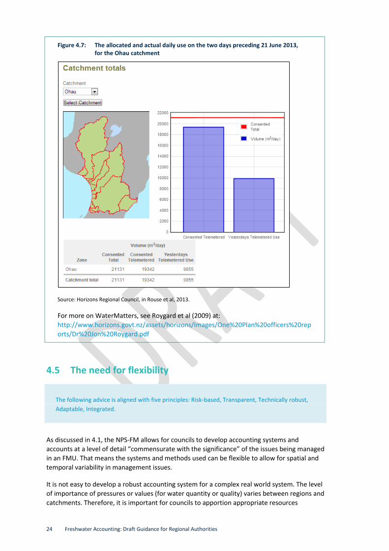
Horizons Regional Council has developed a system that enables it to use telemetry
from metered water takes to produce daily accounts. This information is used to assist
with operational water take compliance and restrictions management.
24 Freshwater Accounting: Draft Guidance for Regional Authorities
Figure 4.7: The allocated and actual daily use on the two days preceding 21 June 2013, for the Ohau catchment
Source: Horizons Regional Council, in Rouse et al, 2013.
For more on WaterMatters, see Roygard et al (2009) at:
http://www.horizons.govt.nz/assets/horizons/Images/One%20Plan%20officers%20rep
orts/Dr%20Jon%20Roygard.pdf
4.5 The need for flexibility
The following advice is aligned with five principles: Risk-based, Transparent, Technically robust,
Adaptable, Integrated.
As discussed in 4.1, the NPS-FM allows for councils to develop accounting systems and
accounts at a level of detail “commensurate with the significance” of the issues being managed
in an FMU. That means the systems and methods used can be flexible to allow for spatial and
temporal variability in management issues.
It is not easy to develop a robust accounting system for a complex real world system. The level
of importance of pressures or values (for water quantity or quality) varies between regions and
catchments. Therefore, it is important for councils to apportion appropriate resources

Freshwater Accounting: Draft Guidance for Regional Authorities 25
depending on the significance of their issues, to optimise the cost-benefit of any accounting
exercises. For example, while high frequency water sampling may be needed to assess nitrate
concentration in a highly developed agricultural catchment to manage water quality, such an
intense monitoring system may be unnecessary for a catchment that is near its natural state.
A sensible approach may be to begin with a simple system for accounting, allowing for
methods and the system itself to improve with time. A good example is the approach taken by
Horizons Regional Council, which developed a simple accounting system to identify the
catchments, rivers and aquifers that required more accurate estimates. More detailed
scientific and technical studies were then conducted on these ‘hotspots’ to improve
understanding of the water quality.
More information about using a flexible, risk-based approach to select methods appropriate
for different types of water takes (eg, permitted or consented) and different sources of
contaminants is provided in 5.2 and 5.3.
CASE STUDY 4.7 – APPROACHES TO ENVIRONMENTAL FLOW SETTING
Horizons Regional Council used an explicitly risk-based approach for selecting methods
to set minimum flows and core allocation limits for its water management zones and
sub-zones. It has developed a decision support framework and identified six
‘scenarios’ that may require the use of different techniques. These range from robust
techniques, such as physical habitat modelling, to default methods using percentages
of a river’s mean annual low flow (MALF). For more on Horizons’ approach to flow
setting, see Roygard et al (2009) at:
http://www.horizons.govt.nz/assets/horizons/Images/One%20Plan%20officers%20rep
orts/Dr%20Jon%20Roygard.pdf.
Otago Regional Council uses physical habitat modelling as one of the key science
components to setting minimum flow requirements for its catchments. At present,
IFIM (physical habitat modelling) is the approach used, mostly because there are few
alternatives at a similar cost. Habitat modelling is both data and time intensive,
which means these studies can be relatively expensive. However, Otago rivers are
either heavily relied on for water abstraction or contain high fisheries value (both
sports fish and native fish), which means the risks are high and more detailed methods
are justified.
To set allocation limits, hydrological alteration, surety of supply, and actual take
information are considered as part of the minimum flow process. Actual takes are
accounted for through summing the water use data collected under the national water
metering regulations or consent conditions.
Technical reports supporting Otago Regional Council’s approach can be found on its
website:
http://www.orc.govt.nz/Utils/Search/?whole=true&query=aquatic+ecosystems.
In summary, allowing for flexibility is important when determining what accounting method to
use. The method should be able to change as circumstances change. As discussed in 4.1, it may
be appropriate to use a risk-based approach: first carry out a scoping exercise, and then devise
an appropriate approach for the region. The general approach might then be:

26 Freshwater Accounting: Draft Guidance for Regional Authorities
measure where required in high priority areas
estimate where order of magnitude is sufficient
model (with validation) where measurements are not possible and/or detailed predictions
are needed.
In practice, methods for measuring consented water takes may differ from methods used to
estimate certain permitted uses. Whatever methods are used, it is important to ensure they
can produce water accounts in a manner consistent with the freshwater objectives set for the
FMU. Furthermore, accounting information for an FMU or catchment may need to feed into
regional accounting systems to allow comparisons between FMUs, and may in the future be
useful for national reporting.
CASE STUDY 4.8 – BEING PRECAUTIONARY WHEN USING ESTIMATES
If robust measurements are unavailable, it may make sense to be conservative in
producing estimates. Waikato Regional Council used this approach in determining
allocable surface water flows. It developed a default approach to setting the allocable
flow component of water quantity limits, using a statistic (10% of Q5)6 as the allocable
flow for the streams when minimum flows are not set using a more detailed scientific
study of instream flow requirements. As the Council learns more about stream
hydrology through scientific studies of similar streams, it has allowed for flexibility to
increase the percentage of allocable flow for some streams (J. Smith, Waikato Regional
Council, pers. com.). Statistical methods are useful in migrating information from
different scales, such as the size of a catchment.
4.6 Comments on using models
The following advice is aligned with four principles: Technically robust, Effective and relevant,
Adaptable, Integrated.
The well-known adage, “you can’t manage what you don’t measure”, is largely true. But, as
outlined in 4.5, for the sake of practicality it is unfeasible to measure everything, at least not
all the time. For example, some measurements, particularly water quality concentration
measurements, are expensive to collect or analyse, and can cost hundreds of dollars per
sample. It is therefore common practice is to use models to help obtain information that we
are unable to, or choose not to measure.
Models can also be used as a predictive tool, especially for exploring scenarios for different
possible futures. For example, an integrated groundwater-surface water model can be used to
predict the future effects of water quality in a river (say in 50 years’ time) due to different
scenarios of land-use change. A third use of models is to better understand complex systems,
6 Q5 – the 7-day low flow which has 20 per cent probability of occurring in any one year (1-in-5 year return
period). A 7-day annual flow minima is the lowest average flow over seven consecutive 24 hour periods for each
complete year of flow record.

Freshwater Accounting: Draft Guidance for Regional Authorities 27
such as when there are significant surface water-groundwater interactions with lag times that
we need to better understand in order to set limits. As summarised by Motu (2013), the
processes that determine nutrient loss, transportation and concentration are complex. This
complexity arises from spatial variability of soil, topography and land use; and temporal
variability of climate, land management practices and nutrient transport beneath the ground.
There are two broad categories of models (Motu, 2013). Theoretical or conceptual models
emphasise the key components of a system and their interactions without seeking to quantify
the magnitude of any component or interaction (they are not quantitative). Numerical or
computer models provide representations of reality that both describe how the different parts
of the model interact, and quantify the magnitude of the different interactions. In practical
modelling systems, data is essential for testing and validating models.
As stated by George Box, “All models are wrong, but some are useful” (quoted in Motu, 2013).
It is important to remember that models are abstract representations of reality and that they
necessarily contain important assumptions and limitations. Furthermore, the amount of data
and information available to construct a robust model can also be limited. It is therefore
important to be open about the design and inherent assumptions used in a model, because if
its structure and input data are inaccurate or uncertain, this will be directly reflected in the
model’s outputs. Being transparent and expressing the assumptions, limitations, error and
uncertainty associated with predictions is an essential part of using models. It is important to
understand these limitations, particularly when they are to be used to communicate with
communities involved in freshwater management decisions for an FMU (see 4.8).
CASE STUDY 4.9 – TEN TIPS FOR SELECTING MODELS
The following tips are taken from Wyatt et al (2014), and based on advice from the
Envirolink Tools decision support system (DSS) website:
http://tools.envirolink.govt.nz/.
1. Clearly define the questions you need the model, tool or DSS to help answer.
2. Define the requirements of the decision-making process you intend to follow
(timeframes, resources, community participation).
3. Understand how the information provided by a tool, model or DSS will need to be
presented to be useful for the community engagement and decision-making
process you intend to follow.
4. Understand the underlying assumptions and limitations of the tool, model or DSS
– can you live with these when explaining results and trying to create consensus in
decision-making?
5. Understand what data and technical expertise is required to run the tool, model
or DSS – can you provide or source these?
6. Check if there are additional costs involved in using the tool, model or DSS, such
as software or licencing.
7. See how easy the tool, model or DSS is to use – can it be readily included into an
existing decision-making process?
8. Check to see if there is support for learning about, setting up and using the tool,
model or DSS (documentation, case studies, New Zealand examples/users).
28 Freshwater Accounting: Draft Guidance for Regional Authorities
9. Understand the 'maturity' of the tool, model or DSS – new and emerging DSS’s
may require more resourcing to learn and implement.
10. Do more homework – take time to explore options and to understand the merits
of using different approaches and DSSs.
4.7 Estimating accuracy and uncertainties
The following advice is aligned with four principles: Transparent, Technically robust, Effective and
relevant, Adaptable.
Measurements and estimates are inherently associated with errors in that they are inaccurate
(they vary from the ‘true’ value) and contain uncertainty (there is some level of confidence in
how well the estimate reflects the ‘true’ value). This uncertainty arises due to many factors
such as limited or missing data, poor quality data, conceptual and structural errors of a model,
and boundary condition errors. The expression of uncertainty for an estimate represents the
compounding errors of data and the model itself.
It is also important to recognise that modelling uncertainty and predictive uncertainty are not
the same thing. Modelling uncertainty can be quantified and represents the imperfect fit of the
estimates or predictions to reality. Predictive uncertainty arises from extrapolation errors.
Future predictions made using a model often have high uncertainty as the future typically does
not look like the past – for example, future flow predictions may be uncertain due to the
effects of climate change.
It is vital to express an uncertainty for all estimated values because decision-makers and
stakeholders need to understand it when considering the information. In other words, the
uncertainty signals the level of confidence that they can place on the information. To this end,
an estimate produced by a model or similar methodology is only complete if it is accompanied
by a statement of the uncertainty. This uncertainty is often expressed as a statistical measure
(for example, a standard error). It is also important to understand the impact that these
uncertainties can have on the decision-making process. For instance, in high priority FMUs
with issues of over allocation, it may be necessary to reduce the uncertainties in order to
provide the necessary confidence in the outcomes of decisions.
In situations where decisions have to be made despite high levels of uncertainty, additional
processes should be put in place to manage the associated risk. For instance, it may be
appropriate for a programme of work to be outlined, whereby over time uncertainties can be
reduced and estimates refined (for example, through improved input data as a result of better
monitoring practices) to enable the future review of decisions that have been made.

Freshwater Accounting: Draft Guidance for Regional Authorities 29
CASE STUDY 4.10 – QUALITY ASSURANCE FOR HYDROLOGICAL DATA
Agencies that collect hydrometric data generally operate under a quality management
system – that is, a set of rules to direct and control an organisation with regard to
quality. It may include a policy or strategy, but more than anything, quality
management is a process. Water data collection and archiving can be managed in a
number of ways to assure the quality of the end product. For example, staff training,
technical competence, good measurement practices, standard
operating procedures/methods, proper facilities and equipment, calibration and
maintenance of equipment, data checking (such as correcting gaps or spikes in a data
series), system improvements and, finally, internal and external audits. There are
standards such as ISO 9000, which exist to help ensure quality levels. All councils
operate Quality Assurance (QA) and Quality Control (QC) systems, which are being
formalised through the National Environmental Monitoring Standards (NEMS)
initiative (see case study 4.11).
Environment Canterbury and Otago Regional Council are in the early stages of
developing QA and QC systems for telemetered water metering data (under the
water metering regulations). The checks are currently limited to assessing spikes and
gaps in data. Environment Canterbury has developed a detailed approach that needs
the water meters and associated telemetry equipment to be installed by accredited
organisations, which ensures that the ±5% accuracy requirement of the water
metering regulations is signed off by an industry certified water meter installer
(M. Ettema, Environment Canterbury, pers. comm).
Horizons Regional Council has also developed requirements for water meter
installation. Further details can be found at:
http://www.horizons.govt.nz/assets/publications/managing-our-
environment/publications-consents/HRC-Watermeter-Brochure-12pg-FIN.pdf.
CASE STUDY 4.11 – NATIONAL INTIATIVES TO HELP STANDARDISE ENVIRONMENTAL DATA
Several initiatives currently being developed will continue to improve and standardise
environmental data collection.
As described in 2.3, both the water metering regulations and Environmental
Monitoring and Reporting (EMaR) are soon likely to require information fundamental
to regional water accounting to also be reported at national level.
Land and Water Aotearoa (LAWA) has expanded from being a collaboration between
New Zealand’s 17 regional and unitary councils, and is now a partnership between the
councils, Cawthron Institute, MfE and Massey University, and has been supported by
the Tindall Foundation. The website hosts environmental data from across the
country, which is quality assured and archived. A user-friendly interface allows simple
graphing and exploration of the data, and fact sheets offer more information on key
topics (see case study 4.12).

30 Freshwater Accounting: Draft Guidance for Regional Authorities
The National Environmental Monitoring Standards (NEMS) steering group has
prepared a series of environmental monitoring standards with support from the
Regional Chief Executive Officers and the Ministry for the Environment. The
development of these standards was led by regional and unitary councils from across
New Zealand, in partnership with the electricity generation industry and NIWA. These
documents prescribe technical standards, methods and other requirements associated
with the continuous monitoring of a number of environmental parameters. Drafts are
currently under development for a number of topics, including water level recording,
open channel flow measurement, water temperature, turbidity, and dissolved oxygen.
See: http://www.lawa.org.nz/ for more on LAWA and NEMS;
http://www.mfe.govt.nz/more/environmental-reporting/about-environmental-
reporting-nz/our-environmental-reporting-programm-0.
4.8 Presenting information to your communities
The following advice is aligned with four principles: Transparent, Effective and relevant,
Partnership, Adaptable.
Under the framework established by the NPS-FM, freshwater management may be
approached in a collaborative way, and many councils are already exploring how to do this. If
freshwater objectives and limits are to be set as part of a collaborative process, then any
accounts produced need to be understandable to a non-technical audience. While the NPS-FM
does not require collaborative processes to be used in this way, Policy CC2 requires councils to
take, “… reasonable steps to ensure that information gathered … is available to the public,
regularly and in a suitable form”.
Some tips to help address this requirement include:
Make sure the purpose of the accounts is clear – which of the four key reasons for
accounting outlined in 2.2 are you currently addressing? What are the main issues driving
your need to account?
Be clear what FMU and which time period the accounts refer to.
Avoid jargon and acronyms as far as possible.
If frequently used technical terms cannot be avoided, introduce and explain each one and
use them consistently.
Use every day analogies if these help communicate complex ideas.
Use visuals (for example, bar or pie charts), as well as tables of figures.
Provide clear explanatory notes on methods and assumptions used, and uncertainties and
limitations associated with data.
Provide sources for further information for those who might be interested in finding out
more.

Freshwater Accounting: Draft Guidance for Regional Authorities 31
CASE STUDY 4.12 – COMMUNICATING IN COLLABORATIVE LIMIT-SETTING PROCESSES
In a broader freshwater management context, different councils and researchers are
exploring different ways to communicate complex science information to communities
as part of collaborative limit-setting processes. Examples include ‘traffic light’ tables
or wheels, which use colours to indicate the extent to which different (often
conflicting) freshwater objectives are being met. See section 5.6.1 of Wyatt et al
(2014) for more information.
Two other examples of communicating environmental data to the community are
state of the environment (SOE) report cards, and the LAWA website. Councils have
been reporting SOE results to their communities for many years, and have developed
many types of ‘report cards’ to simplify this complex information. For example,
Auckland Council produces report cards for its SOE monitoring, including fresh water,
for different reporting areas. An overall grade is given to the area, based on water
quality, flow patterns, nutrient cycling, habitat quality, and biodiversity. A catchment
map, photo and quick facts are given, as well as the overall grade, and grades for the
five indicators. The report cards are available online and downloadable as a PDF. For
more information, see: http://stateofauckland.aucklandcouncil.govt.nz/report-
type/freshwater-report-card/.
One of the key aims of LAWA (introduced in case study 4.11), is to help local
communities find out more about their fresh water. The LAWA website allows
someone to explore data, selecting a region and then a catchment area. Figure 4.8 is
taken from the Ashburton River at a State Highway 1 site and shows the median state
of a number of environmental indicators compared to other sites, and trend
information based on 9-year data. See: http://www.lawa.org.nz/explore-
data/canterbury-region/ashburton-river/ashburton-river-at-sh1/.
Figure 4.8: Snapshot of water quality data for the Ashburton catchment, from the LAWA website

32 Freshwater Accounting: Draft Guidance for Regional Authorities
5 Key components of accounting systems
5.1 The key components of accounting
Figure 5.1 outlines the key components of freshwater accounting, showing stages that are
common, as well as ones that are specific to either water quantity or quality accounting.
Figure 5.1: Key components of freshwater accounting for water quantity and quality
Note: M, E, M = measure, estimate or model.
Define what you are accounting for, the purpose, and the units to be used
Define freshwater management unit
Bringing it all together – system requirements
Reporting – using a suggested template
Account for each type of take (M, E, M)
Establish current (measured) state
Reconcile measured and estimated (refine estimates)
Account for each relevant source of contaminants (M, E, M):
natural sources
consider attenuation
consider lag
Water quantity Water quality

Freshwater Accounting: Draft Guidance for Regional Authorities 33
This section steps through specific requirements for water quantity (5.2) and water quality
(5.3) accounting.
The NPS-FM requires councils to use the National Objectives Framework (NOF) to help set
freshwater objectives and limits for a freshwater management unit (FMU). There is a degree of
overlap with methods that help with accounting, and the methods used to set freshwater
objectives and limits. Here we focus on accounting, and, where possible, refer readers to other
sources of information about limit setting and collaborative planning approaches.
5.2 Water quantity
5.2.1 Define what you are accounting for
Identifying all water takes
The first stage of water quantity accounting is to define and establish what is being accounted
for. There are many different types of water takes, and the NPS-FM requires councils to
account for them all. One useful approach is to separate the types of take based on their
characteristics.
Because councils have managed different types of water take as business-as-usual before the
NPS-FM required accounting, they are likely to have a thorough understanding of the topic.
However, this section outlines the different types of take to ensure this guidance offers a
complete package, and to reflect the important role they play in the later stages of water
quantity accounting.
Water takes can be defined in three ways, described below:
Consumptive or non-consumptive use
Consumptive water use is when water is removed from a water body for a purpose and is not
returned to the water resource system, such as water used for irrigation and domestic supply
purposes. Strictly speaking, there is always some level of return to the water cycle. For
example, irrigation water that is transpired during plant growth, and the deep drainage
component discharged to the groundwater. However, these returns are generally small, can
occur with significant time lag, and may not be returned back to the same water body that the
water was originally abstracted from, or be of the same quality it was when abstracted.
Therefore, once removed from a water body, consumed water is not available for reuse.
Non-consumptive water use (such as that defined in regulation 4(2) of the water metering
regulations) includes water withdrawn for use, but returned directly back to the source with a
relatively short return time lag. For example, water withdrawn for purposes such as
hydropower generation is generally non-consumptive. However, there is still potential for a
reduction in water quality to occur as a result of the water being unavailable for immediate
reuse. For example, water abstracted for cooling purposes may increase in temperature, which
may affect immediate reuse. It is important to account for both consumptive and non-
consumptive takes for informing the setting of objectives and limits. For example, while a non-
consumptive take (such as a hydro-generation dam) may not affect the downstream
availability of water, any upstream consumptive takes may affect the ability for the dam to
operate effectively.

34 Freshwater Accounting: Draft Guidance for Regional Authorities
As consumptive water takes result in water being removed from a water body and a
reduction in available water volume (over a reasonable timeframe), it is important that water
accounting systems clearly differentiate between consumptive and non-consumptive takes.
Where only a portion of the take is returned to the source, a freshwater quantity accounting
system should clearly identify the volume available for reuse in a non-consumptive take to
help ensure water resources are managed efficiently.
Consented takes
The RMA stipulates that a resource consent is needed for the take and use of water, although
there are exceptions to this (these are discussed under ‘unconsented takes’ below). Consent
can be required for both consumptive and non-consumptive takes. Consented takes are likely
to represent the highest proportion of water use in many FMUs. Therefore, accurate and
appropriate information about consented takes is critical for water accounting. Information
stored in a consent database is essential for many facets of water management and reporting
where it may be used to avoid over allocation, improve water use efficiency, protect wetlands,
check for compliance with consent conditions, and provide input to SoE reporting, as well as
for freshwater accounting purposes.
It may be appropriate and pragmatic to use consistent fields in a consent database, noting that
regional flexibility to allow fit-for-purpose management is also important. New accounting
requirements may mean there is a need to review and improve the consent information
collected. The suggested list of fields below is for guidance only – councils may use only those
they determine as necessary, or add more fields as required to meet FMU or regional
circumstances. A certain level of standardisation is important to enable computer-based
systems of data storage and retrieval.
The potential fields for a consent database are:
Consent identifier (number).
FMU.
Consumptive or non-consumptive.
Primary source (eg, groundwater or surface water).
Source type (eg, river, storage).
Source catchment (eg, Hurunui River catchment).
Source name (eg, Waikato River, Kaawa aquifer).
Primary use.
Secondary use (eg, stock water when the primary use is irrigation).
Use type (eg, pasture irrigation, vegetable irrigation, cooling).
Description of use.
Instantaneous rate (ℓ/s).
Daily volume (m3/d).
Weekly volume (m3/week).
Seasonal volume (m3/season) (eg, for irrigation, if specified).
Annual rate (m3/year).
Take months (eg, October to April for irrigation).

Freshwater Accounting: Draft Guidance for Regional Authorities 35
Irrigated area (ha).
Discharge/return volume (may need to use more fields if necessary to account for
accurate net use – ie, ℓ/s, m3/d and m3/year may be required as separate fields).
Transfer volume (may need to use more fields if necessary to account for accurate transfer
– ie, ℓ/s, m3/d, m3/year period of the transfer, transfer location, etc, may be required as
separate fields).
Surface water/groundwater interaction apportion (eg, assign 20 per cent of a groundwater
take to a nearby stream. May need more fields and association with other FMUs, if
interaction is high – see 5.2.3 for further details).
Map reference7 (ie, Easting and Northing).
Consent commencement date.
Consent expiry date.
Water meter installed (eg, yes or no).
Commencement date of water meter reading.
In future, a field may be required to record restrictions to taking water that may be
introduced.
Unconsented takes
Section 14(3)(b) of the RMA permits the take and use of water for certain activities without the
need to obtain a resource consent. These are known as ‘permitted takes’. These permitted
takes allow for water to be taken for an individual's reasonable domestic needs and stock
water, provided that the use does not, or is not likely to, have an adverse effect on the
environment.
To implement the RMA statutory requirements, councils often specify in a regional plan a
quantity of water that can be taken without a resource consent. Case law has confirmed that
this is a legitimate practice.
There are also potentially unauthorised takes that are not permitted under the RMA or a
regional/district plan, that exceed the consented volume or permitted activity rule, or where
an old consent has expired. It is important that the source (groundwater or surface water) of
the unconsented take is identified and classified and assigned against the appropriate FMU.
The common unconsented water take types are:
permitted takes under RMA S14(3)(b)
permitted takes under regional/district plans
unauthorised takes.
Understanding water resource availability
For accounting where limits have been set, the types of takes outlined above are likely to be
the only things that need to be accounted for. However, for accounting where limits have not
7 Remembering to check that grid reference matches the position of the actual take, if this is not the same as
consented.

36 Freshwater Accounting: Draft Guidance for Regional Authorities
yet been set, councils may also need to know more about the water resource itself. For surface
water bodies, such as rivers, to set limits for resource use as required by the NPS-FM, a key
step is to determine minimum flow requirements (the flows required to maintain instream
values). These could include ecological values, recreational values, amenity and natural
character values, and tangata whenua values (Beca, 2008) as well as the assimilative capacity
for other contaminants. Councils have been undertaking such analyses for some time, and
advice already exists on these topics. However, until recently, not all councils had taken the
next step to establish allocation limits, though this is becoming more widespread (Rouse et al,
2013; Rouse and Norton, 2013). Naturalised flow series (ie, assuming no abstraction, damming,
diversion, or discharge) are generally used for establishing minimum flow requirements and
allocation limits.
CASE STUDY 5.1 – GUIDANCE ON METHODS FOR SETTING ENVIRONMENTAL FLOWS
Two main documents can help councils set environmental flows:
Flow guidelines for instream values (Ministry for the Environment, 1998a and
1998b).
Draft guidelines for the selection of methods to determine ecological flows and
water levels (Beca, 2008).
Case study 4.1 (section 4) discusses how a risk-based approach can be used to guide
the selection of these methods. The Draft guidelines (Beca, 2008) focus on methods to
address ecological values. The Flow guidelines for instream values also discuss these
values, along with methods to address recreational, amenity and natural character,
and tangata whenua values.
For groundwater, a common and appropriate method for determining sustainable aquifer
yields is to develop an integrated groundwater-surface water model. Developing an accurate
groundwater model requires a large amount of data and information, and it may be
appropriate to first develop a basic (conceptual) groundwater model to identify where data
gaps exist. The development process may therefore require a reasonable period of time. Basic
approaches, such as percentage of average annual rainfall as an annual sustainable yield, can
be used in the absence of an accurate modelling approach. However, a cautious approach
should be used to arrive at conservative estimates when using simple methods as it may take
centuries to recharge a groundwater system that has been over extracted. The Draft guidelines
(Beca, 2008) describe methods for deciding appropriate groundwater minimum levels.
CASE STUDY 5.2 – SETTING GROUNDWATER LIMITS
Tasman District Council uses an integrated groundwater-surface water model for
managing the water of the coastal Motueka-Riwaka Plains. The primary purpose of the
model is to ascertain the sustainable yield from the aquifer system while maintaining
depletions of the nearby Motueka River and springs within allowable limits (as
stipulated in the District Plan) and preventing saltwater intrusion (Aqualinc, 2008).
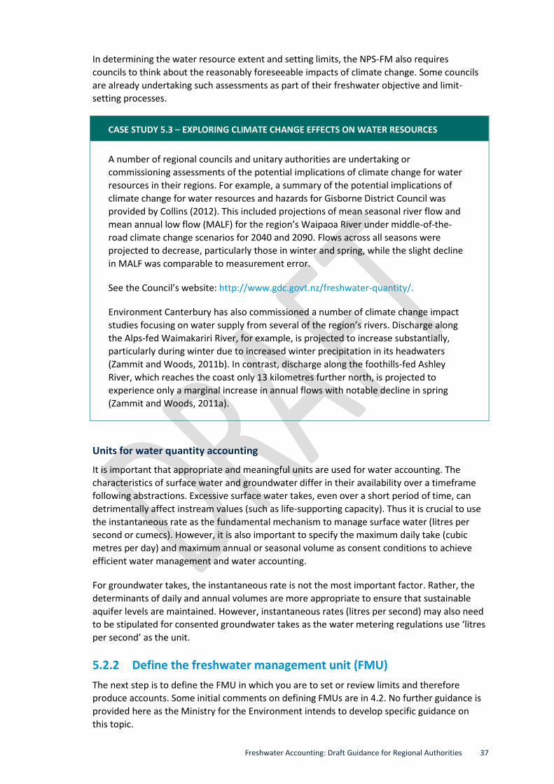
Freshwater Accounting: Draft Guidance for Regional Authorities 37
In determining the water resource extent and setting limits, the NPS-FM also requires
councils to think about the reasonably foreseeable impacts of climate change. Some councils
are already undertaking such assessments as part of their freshwater objective and limit-
setting processes.
CASE STUDY 5.3 – EXPLORING CLIMATE CHANGE EFFECTS ON WATER RESOURCES
A number of regional councils and unitary authorities are undertaking or
commissioning assessments of the potential implications of climate change for water
resources in their regions. For example, a summary of the potential implications of
climate change for water resources and hazards for Gisborne District Council was
provided by Collins (2012). This included projections of mean seasonal river flow and
mean annual low flow (MALF) for the region’s Waipaoa River under middle-of-the-
road climate change scenarios for 2040 and 2090. Flows across all seasons were
projected to decrease, particularly those in winter and spring, while the slight decline
in MALF was comparable to measurement error.
See the Council’s website: http://www.gdc.govt.nz/freshwater-quantity/.
Environment Canterbury has also commissioned a number of climate change impact
studies focusing on water supply from several of the region’s rivers. Discharge along
the Alps-fed Waimakariri River, for example, is projected to increase substantially,
particularly during winter due to increased winter precipitation in its headwaters
(Zammit and Woods, 2011b). In contrast, discharge along the foothills-fed Ashley
River, which reaches the coast only 13 kilometres further north, is projected to
experience only a marginal increase in annual flows with notable decline in spring
(Zammit and Woods, 2011a).
Units for water quantity accounting
It is important that appropriate and meaningful units are used for water accounting. The
characteristics of surface water and groundwater differ in their availability over a timeframe
following abstractions. Excessive surface water takes, even over a short period of time, can
detrimentally affect instream values (such as life-supporting capacity). Thus it is crucial to use
the instantaneous rate as the fundamental mechanism to manage surface water (litres per
second or cumecs). However, it is also important to specify the maximum daily take (cubic
metres per day) and maximum annual or seasonal volume as consent conditions to achieve
efficient water management and water accounting.
For groundwater takes, the instantaneous rate is not the most important factor. Rather, the
determinants of daily and annual volumes are more appropriate to ensure that sustainable
aquifer levels are maintained. However, instantaneous rates (litres per second) may also need
to be stipulated for consented groundwater takes as the water metering regulations use ‘litres
per second’ as the unit.
5.2.2 Define the freshwater management unit (FMU)
The next step is to define the FMU in which you are to set or review limits and therefore
produce accounts. Some initial comments on defining FMUs are in 4.2. No further guidance is
provided here as the Ministry for the Environment intends to develop specific guidance on
this topic.

38 Freshwater Accounting: Draft Guidance for Regional Authorities
5.2.3 Account for each type of take
The NPS-FM requires accounting for all water takes: consented (including both consumptive
and non-consumptive), permitted and unauthorised takes. As outlined in 5.2.1, if accounting
information is being used to inform limits, information on the available water resource (river
flows or groundwater levels) will also be required.
At present, it is more likely that accurate information will be available for consented
consumptive takes, both what is allocated and what is used (at least for takes greater than
20 litres per second due to the current water metering regulations). It may therefore be
appropriate for consented takes to be accounted for separately from unconsented takes.
Accounting for the total water use from unconsented and non-consumptive takes will most
likely require the use of estimates or models, as it is unusual for water measurements to be
available for these takes. One-off measurements of unconsented takes may be useful to
improve or validate the assumptions used in any estimates or models.
Consented takes
Some comments on allocation
As stated in 5.2.1, consented takes are likely to represent the highest proportion of water use
within an FMU. Accurate checks and balances for consented takes are therefore essential for
water accounting and to ensure resources are not over-allocated.
Surface water availability at a given location may not be solely determined by the availability
within the (sub) catchment containing that location. This is because allocation of water in an
upstream sub-catchment will reduce the availability within lower catchments. For example, in
the Upper Waikato Catchment, the catchment is fully allocated at the Karapiro Dam. Although
there is allocable water within a number of upper sub-catchments when assessed in isolation,
this water cannot be allocated as the water resource for the lower catchment at Karapiro Dam
is fully allocated. Thus accounting systems need to be able to help councils understand how
takes from one location in an FMU may impact takes in other parts. This is necessary for
considering limits to avoid over-allocation (see case study 5.7 for more information). Where
possible, this issue should be considered when FMU boundaries are being defined.
The allocation to non-consumptive takes can also determine the availability for consumptive
use, rather than instream minimum flow requirements (eg, for ecological values). This is the
case in the Upper Waikato Catchment, where water availability for consumptive takes within
the catchment is primarily established based on non-consumptive takes for hydropower
generation for the eight power stations located on the river.
Water quantity accounting can become complex when non-consumptive takes are partly
consumptive. For example, Huntly power station takes 40 cumecs for cooling and returns 38
cumecs. Therefore, councils need to understand the initial take and the return, and thus the
net take in their accounting.
Actual use
The water metering regulations require all water consents that authorise water takes at a
rate of 5 litres per second or more (with the exception of non-consumptive take as defined
by the regulations) to record their actual water abstraction, and report this data annually to
the council. These regulations initally only applied to takes of 20 litres per second or more.
From 10 November 2014, they have applied to takes of between 20 and 10 litres per second.

Freshwater Accounting: Draft Guidance for Regional Authorities 39
From 10 November 2016 they will apply to takes of between 5 and 10 litres per second. If
appropriate consent conditions, recording, reporting, storing and compliance systems are in
place, councils should be able to produce accurate annual water accounts for the consented
takes of 5 litres per second or more with relative ease.
CASE STUDY 5.4 – USE AND DISPLAY OF TELEMETERED WATER USE DATA
Horizons Regional Council has installed telemetry systems on water meters in its
region and captures close to real time data. The data are displayed through its Water
Matters website, which is, “… a web-based information system for individual consent
holders and those organisations in the region interested in water management. It
allows individual consent holders to monitor their water use from their computer at
home, and it allows whole water management zone monitoring against predetermined
water allocation limits”. An example screenshot is shown in figure 5.2 and more can be
found at: http://www.horizons.govt.nz/managing-environment/resource-
management/water/watermatters/watermatters-overview/.
Figure 5.2: Screenshot from Water Matters from the Rangitikei catchment, July 2014
Through consent conditions Otago Regional Council has had telemetry systems
installed on all water takes from the Kakanui River greater than 5 litres per second to
allow real time water management for the catchment’s water users during times of
low flow. The data are displayed through an independent provider’s website where
individuals can view their own water use on their home computer while the
catchment’s water allocation committee can view all water users’ data, allowing it to
make real time decisions during times when sharing is necessary to meet minimum
flow expectations. The screenshot in figure 5.3 shows the rate of take and monthly
volume used for a water take in the Kakanui River.

40 Freshwater Accounting: Draft Guidance for Regional Authorities
Figure 5.3: Screenshot of the rate of take and monthly volume used for a water take in the Kakanui River
As discussed in section 4, while the water metering regulations require consent holders to
provide annual returns, councils may require more frequent data collection to meet their
commitments to implement the NPS-FM, especially for surface water takes. Real time data
collection (for example, using telemetry) may be helpful for larger takes and within
catchments and streams that are highly allocated. Councils could consider including
appropriate consent conditions to gather water use data at meaningful frequencies and in
useful formats (such as electronic) to assist them in effective water management. Where net
takes need to be accounted for, both take and discharge (returned water) should be measured
at the same frequency.
As discussed above, at the time of writing, under the water metering regulations, water use
records are available for takes of greater than 20 litres per second, and some regional/district
plans require all consented water takes to be measured, such as in the Waikato region.
Consented takes that are not currently measured need to be estimated for water quantity
accounts. One approach that can be used to account for unmeasured takes is to use pro rata
estimates based on measured takes for similar water uses. For example, an estimate for an
unmeasured consented pastoral irrigation water take could be based on a measured pastoral
irrigation take in an area with a similar microclimate. It is also important to use data from
similar soil types (where the soils’ plant-available water is similar) and where irrigation
management practices are similar. However, it may be difficult to find exact matching
1-Jan-2014 29-Jan-2014 26-Feb-2014 26-Mar-2014
0.0
2.0
4.0
6.0
8.0
10.0
12.0
14.0
16.0
18.0
20.0
1-Jan-2014 00:00:00 to 1-Apr-2014 00:00:00
Pump Flow (l/s) at Kakanui Water Take
Abstraction rate shall not exceed 18L/s
Ta
ke (
l/s)
1-Jan-2014 29-Jan-2014 26-Feb-2014 26-Mar-2014
0
5000
10000
15000
20000
25000
30000
35000
40000
45000
1-Jan-2014 00:00:00 to 1-Apr-2014 00:00:00
Volume - Monthly at Kakanui Water Take
Abstraction vol. shall not exceed 39,500m3/month
Volu
me taken
(m3)

Freshwater Accounting: Draft Guidance for Regional Authorities 41
conditions between takes for all purposes, and a number of assumptions may need to be
made. Another possible way for estimating water use from groundwater takes is by using the
power consumption of pumps as a proxy measure for the water abstracted. For all such
estimates, uncertainties can be high and it is important that the accounts clearly express these.
Permitted takes
As permitted activities (either under RMA s14(3)(b) or under regional/district plans) do not
require resource consents, councils generally do not have detailed information about
actual permitted use, such as the location of the take, water source and purpose of the take.
However, under the NPS-FM, councils are required to estimate the amount of this permitted
water use in their accounts. It may be helpful to do this by source (ie, groundwater or
surface water).
To manage water resources sustainably, councils need a reasonably accurate understanding of
the water used under permitted takes, and its significance in comparison to the total resource
available. This is not as important for some areas – for example, on Banks Peninsula in
Canterbury, permitted takes are considered to be minor compared to the consented takes
(T. Davie, Environment Canterbury, pers. com.). However, Waikato Regional Council has found
that the cumulative permitted water use is significant in some catchments, to the extent that it
is placing stress on environmental bottom lines (Waikato Regional Council, 2007). This
reinforces the importance of councils using approaches that are appropriate for the
significance of the issue in their FMUs.
As permitted takes are not generally measured, it is necessary to estimate this use. It is
unlikely that all properties (or their owners) use the maximum authorised amount under the
regional/district plan all the time. For example, Waikato Regional Plan authorises use of up to
15 cubic metres a day per property. Therefore, estimates need to be made using reasonably
accurate demands within an FMU, such as domestic (using population figures), stock water
(using stock numbers), and associated demands (including dairy shed demands that do not
require a consent) and small irrigation activities (in rural residential areas).
It is important that councils develop a pragmatic and defensible approach for estimating
permitted water use that can be updated with relative ease.
CASE STUDY 5.5 – ESTIMATING PERMITTED TAKES
Waikato Regional Council has developed a model for estimating takes permitted by its
regional plan and RMA s14(3)(b) using a geographic information system. The method
uses population (census), livestock (Agribase), property information (Land Information
New Zealand), and river and groundwater bore databases to estimate reasonable
water demands for certain uses, and their potential source (ie, groundwater or surface
water). The model’s accuracy has been tested using water measurements from seven
rural water supply schemes (Waikato Regional Council, 2007).
The report can be found at:
http://www.waikatoregion.govt.nz/Services/Publications/Technical-Reports/A-Model-
for-Assessing-the-Magnitude-of-Unconsented-Surface-Water-Use-in-the-Waikato-
Region/.

42 Freshwater Accounting: Draft Guidance for Regional Authorities
Unauthorised water use
It is possible that there are unauthorised water takes in a region – for instance, where a water
user mistakenly believes their water use is authorised under the RMA/regional plan/district
plan. These takes may be the most difficult to estimate because, by their nature, councils tend
to be unaware of them. One potential unauthorised water use can be for dairy shed wash
down and milk cooling as this can be a permitted activity if the take does not exceed the
maximum amount authorised under the regional/district plan. However, with recent
intensification and increased stocking rates, the water demands for dairy shed wash down and
milk cooling have increased on many dairy farms. Similar water use increases may have
happened in small orchards, nurseries and market gardens, where the users are unaware of
the regional/district rules. Therefore, councils need to assess such potential takes and account
for unauthorised water takes. Councils should also have a strategy to address such
unauthorised takes – such as requiring resource consent or reduction of takes to fall within
permitted take rules.
Assessing databases such as AgriBase (ie, stock numbers) against consented data for both
water takes and discharges, and examining aerial maps and visits to potential water use
properties (that do not have resource consents) are some approaches councils can utilise to
estimate unauthorised water use.
5.2.4 Bringing it all together
System needs
The ultimate objective of the NPS-FM is to provide accounts using all of the components
discussed above. Thus, the next stage is to bring the different threads of information together
to achieve the four intended purposes of accounting, outlined in 2.2.
A freshwater quantity accounting system may be a hybrid system with many components, as
outlined in 5.1. The data and information on the available resource (where limits have been
set), consented amounts (consent database), actual measured water use (water meter), and
estimates of unmeasured water use (unmetered consented takes, permitted takes and
unauthorised takes) may sit in different locations and formats within the council. Some are
likely to be in electronic form, and others, at least at this stage, may be in paper format. The
accounting system should enable these varied information sources to be readily collated.

Freshwater Accounting: Draft Guidance for Regional Authorities 43
CASE STUDY 5.6 – EXAMPLE WATER QUANTITY ACCOUNTING SYSTEMS
Figures 5.4 and 5.5 are two schematics of water accounting systems, taken from Rouse
et al (2013). These systems comprise various consent, SOE monitoring or water
metering databases, linked manually or automatically to a system that enables the
council to generate and display water quantity accounts.
Figure 5.4: Horizons Regional Council’s water quantity accounting system
Figure 5.5: Auckland Council’s water quantity accounting system
Councils will need to produce accounts as necessary for FMUs where freshwater objectives
and limits are being set or reviewed. As this process will be repeated across multiple FMUs it is
worth developing a robust accounting system. The investment needed will depend on regional
circumstances, as some councils currently have more advanced systems than others. As almost
all councils have some form of current system in place (at least to address a part of the
accounting system; see Rouse et al, 2013), it is important that careful consideration is given to
modifying the current system (if required) or, alternatively, to developing a new system. The
most efficient system is likely to be completely electronic, linking water availability and
different uses, which can be updated at regular intervals. This type of system requires
significant investment in metering, telemetry and automatic systems to QA, store and display
the data, and may not be necessary for all regions or FMUs. Where paper data exist that
cannot link directly between different electronic databases/systems, the investment required
for an accounting system is in manually inputting data, system processing, and QA to obtain
meaningful information. This type of system may be appropriate for some FMUs, such as those
at near natural state or with few development pressures.

44 Freshwater Accounting: Draft Guidance for Regional Authorities
CASE STUDY 5.7 – EXAMPLE OF A WATER QUANTITY ACCOUNTING SYSTEM
Waikato Regional Council has developed a Water Allocation Calculator (WAC) for
overall water management. The WAC is an integrated electronic system consisting of
many components:
Catchment – created using minimum flow ecological studies, NIWA’s River
Environment Classification (REC), and a purpose-built ‘tracer tool’. This provides
information on total resource availability by stream/catchment. The database is linked
to all water use types (consented and permitted) to tally total water use against the
availability at any given time. The ‘tracer tool’ enables managing all the sub-
catchments within a large catchment because allocation or use in one part of the
catchment has an impact on other parts (see 5.2.3).
Aquifer – similar to ‘Catchment’, but contains information on sustainable yield,
groundwater recharge, and rainfall recharge.
Consents – all consented takes, including non-consumptive takes. This also includes
information about net use (ie, take – return), and percentage use of surface water and
groundwater for a consent (determined based on knowledge of the resource
interaction).
Permitted takes – estimated permitted takes for human and stock use (see 5.2.3).
The WAC is a dynamic system – one part automatically updates every two hours, and
other parts update daily. The resulting calculations help consent officers understand
water availability within any particular catchment or aquifer when assessing new
water take applications. The tool also helps science and policy staff understand the
overall water allocation status across the region.
Figure 5.6: Waikato Regional Council’s water quantity accounting system
5.2.5 Preparing a report
While the main driver for freshwater accounting is to provide better information for councils
to implement the NPS-FM requirements for limit setting, a nationally-consistent reporting
template could also deliver benefits, including:
communities and regulators could assess the status of their water use against other
regions/FMUs
Timeseriesmanagement
Custom GISSpatial Management
and AccountingIRIS
WISKI(meter info.)In the future
Permitted activity spreadsheet

Freshwater Accounting: Draft Guidance for Regional Authorities 45
the ability to compare water accounts between regions. This may allow stakeholders (eg,
irrigators, industries, investors) to identify the potential regions/FMUs suitable for future
growth, between, as well as within, regions
the ability for central government to more easily compile national accounts, if required in
the future (while noting there is currently no prescription for this).
We include a suggested template in table 5.1 that could be used for regular water quantity
accounting reporting by FMUs. Water exports out of a FMU, which require a consent to take
water (eg, taking water from the Waikato River for the Auckland city reticulated supply) and
discharge (eg, Tongariro Power Scheme discharges water into the Lake Taupo catchment in the
Waikato Region after taking water from the Whanganui River catchment in the Horizons
Region), are covered by this accounting process and need not be specifically identified. If limits
(minimum flows and allocation rates) have been set, these could be inserted into this table and
reported against.
Case studies 2.1, 5.4, 5.5 and 5.6 provide other examples of catchment, regional and national
accounts that could guide councils on what to include in a freshwater quantity account.
Table 5.1: A suggested template for water quantity accounting
FMU Name of catchment or subcatchment, or aquifer
Period Date range (eg, 1 July – 30 June Year)
Location Grid ref (eg, centroid of catchment polygon, or most downstream point)
FMU includes Both SW and GW takes √
SW takes only
GW takes only
Units Million cubic metres per year (Mm3/year)
Total volume of FMU (surface water flow / groundwater quantity) Mm3/year A
Total sustainable yield available for consumptive use Mm3/year B
Non-consumptive takes
Number of consented takes x
Authorised volume (Mm3/year)
Volume used (Mm3/year)
Error estimates (%) Methods used
Consented Measured and/or estimated
Transferred Measured and/or estimated
Consumptive takes
Number of consented takes xx
Authorised volume (Mm3/year)
Volume used (Mm3/year)
Error estimates (%) Methods used
Consented takes C F Measured and/or estimated
Consented discharge
D G Measured and/or estimated
Net consented take E (C-D) H (F-G) Measured and/or estimated
Permitted I Estimated
Unauthorised J Estimated
Transferred Measured and/or estimated
Summary
Volume (Mm3/year) Percentage use (%)
Total net use K (H+I+J) K/B x100
Made available to the environment L (A-K) L/A x100

46 Freshwater Accounting: Draft Guidance for Regional Authorities
5.3 Water quality
5.3.1 Define what you are accounting for
Identifying relevant contaminants
As with water quantity accounting (see previous section), the first stage of water quality
accounting is to define and establish what you are accounting for. The NPS-FM requires water
quality accounting to address all relevant sources of contaminants. Careful consideration
needs to be given when identifying which contaminants are relevant, as there could be major
cost implications if irrelevant contaminants are selected. For example, monitoring of non-
relevant contaminants may result in a reduction of the spatial resolution at which the
monitoring is undertaken. As a first step, it may help to understand whether the contaminants
of concern are conservative or non-conservative. Non-conservative contaminants are those
that are transformed in the environment. Understanding this will help to determine how the
contaminants should be accounted for.
The NPS-FM requires councils to use the NOF to help set freshwater objectives and limits for a
FMU. As freshwater accounting is required for FMUs where freshwater objectives and limits
are being set or reviewed, we briefly look at how some of the NOF features help select
relevant contaminants.
Compulsory values
Appendix 1 of the NPS-FM includes two compulsory national values – ecosystem health and
human health for recreation – for which attributes are listed in its Appendix 2. The attributes
relate to quantifiable aspects of the freshwater environment that councils must monitor and
manage in order to meet the compulsory national values. Table 5.2 lists the attributes relating
to these two compulsory values for both rivers and lakes. For example, to manage ecosystem
health, the National Objectives Framework (NOF) requires the management of total nitrogen
(TN) and total phosphorus (TP), which would need accounting for in an FMU that contains
lakes. Note that Appendix 2 of the National Policy Statement for Freshwater Management is
not fully populated and that additional attributes will continue to be added over time.
Table 5.2: Attributes to be managed under the National Objectives Framework
Compulsory Value Rivers Lakes
Ecosystem health Periphyton
Nitrate (as N)
Ammonia (as N)
Dissolved oxygen (below point sources only)
Phytoplankton (chlorophyll a)
Total nitrogen
Total phosphorus
Human health for recreation E. coli
Planktonic cyanobacteria (lake fed rivers only)
E. coli
Planktonic cyanobacteria
Additional national values
In addition to compulsory values for each FMU where freshwater objectives are being set,
Appendix 1 of the NPS-FM contains optional national values that councils must also consider.
For example, a FMU may be (or contain) a water supply catchment, be culturally significant for
food gathering (mahinga kai), or have particular characteristics that impart high aesthetic
values (eg, glacial lakes (hue), Te Waikoropupu Springs of Golden Bay (clarity)). In cases where
an attribute listed in Appendix 2 for a compulsory value is also relevant to one of these

Freshwater Accounting: Draft Guidance for Regional Authorities 47
optional national values, then these attributes need to be accounted for. For example, E.coli
could also be a relevant attribute for mahinga kai, mahi māra (cultivation), wai tapu (sacred
waters), and wai Māori (water supply). However, it is likely that other attributes, not currently
listed in Appendix 2, may also be necessary to protect these values in a particular FMU. For
example, a FMU that is deemed nationally significant with respect to mahinga kai might lie
within a catchment used for coal mining. In this case it may also be necessary to set freshwater
objectives and limits for suspended sediment and heavy metals, and to include these
contaminants in the freshwater accounts for that FMU.
FMUs that are identified as having national values for fishing may require special consideration
from a water quality standpoint. Such FMUs need to provide sufficient numbers of fish (to
support fishing activity), and may also need to provide fish suitable for human consumption. In
general, the water quality attributes required to support a viable fishery are temperature,
clarity and suspended solids. These attributes are not currently included in Appendix 2 of the
NPS-FM, but if they are considered to be important, contaminants that affect these attributes
will need to be accounted for.
Regional values
The NPS-FM also allows councils to set objectives and limits to protect other values (not
included among the national values in its Appendix 1), which they consider appropriate to their
local and regional circumstances (Policy CA2 b) ii). The setting of such freshwater objectives
and limits will necessitate accounting for the contaminants that impact on the values chosen.
One instance where setting regional values (and unique attributes) will likely arise is in urban
FMUs. For example, in the Auckland Region suspended sediment concentrations and heavy
metals (copper and zinc) have been shown to be important (see case study 5.8), particularly in
estuarine environments. While at first glance, this may appear outside the remit of the NPS-
FM, Policies A1, B1 and Appendix 1 specifically instruct councils to take into account the
connections between water bodies, and connections between freshwater and coastal waters
in particular. Although the majority of the effect of these contaminants is on coastal
ecosystems, the delivery mechanism is freshwater streams and creeks.
CASE STUDY 5.8 – IDENTIFYING ATTRIBUTES IN AUCKLAND STREAMS RELEVANT TO REGIONAL VALUES OF AQUATIC ECOSYSTEMS
A series of major studies by Auckland Regional Council (the predecessor of Auckland
Council) found that stormwater from urban catchments could have serious long-term
impacts on the health of receiving waters (see Mills and Williamson, 2008 for a review
of information up to 2005). Heavy metals, particularly copper and zinc, were
investigated.
Also in 2008, a series of reports was published on the effects of urban stormwater on
the ecosystem health of the Central Waitemata Harbour. One of the outputs of the
study was an assessment of long-term accumulation of sediment, copper and zinc in
large-scale harbour depositional zones. The potential for adverse ecological effects
from copper and zinc in the harbour sediments was assessed against sediment quality
guidelines for chemical contaminants. Other tools assessed the effects of different
stormwater management interventions on sediment and stormwater chemical
contaminant accumulation in the central harbour over a 100-year period.
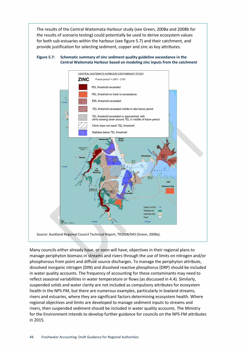
48 Freshwater Accounting: Draft Guidance for Regional Authorities
The results of the Central Waitemata Harbour study (see Green, 2008a and 2008b for
the results of scenario testing) could potentially be used to derive ecosystem values
for both sub-estuaries within the harbour (see figure 5.7) and their catchment, and
provide justification for selecting sediment, copper and zinc as key attributes.
Figure 5.7: Schematic summary of zinc sediment quality guideline exceedance in the Central Waitemata Harbour based on modeling zinc inputs from the catchment
Source: Auckland Regional Council Technical Report, TR2008/043 (Green, 2008a).
Many councils either already have, or soon will have, objectives in their regional plans to
manage periphyton biomass in streams and rivers through the use of limits on nitrogen and/or
phosphorous from point and diffuse source discharges. To manage the periphyton attribute,
dissolved inorganic nitrogen (DIN) and dissolved reactive phosphorus (DRP) should be included
in water quality accounts. The frequency of accounting for these contaminants may need to
reflect seasonal variabilities in water temperature or flows (as discussed in 4.4). Similarly,
suspended solids and water clarity are not included as compulsory attributes for ecosystem
health in the NPS-FM, but there are numerous examples, particularly in lowland streams,
rivers and estuaries, where they are significant factors determining ecosystem health. Where
regional objectives and limits are developed to manage sediment inputs to streams and
rivers, then suspended sediment should be included in water quality accounts. The Ministry
for the Environment intends to develop further guidance for councils on the NPS-FM attributes
in 2015.

Freshwater Accounting: Draft Guidance for Regional Authorities 49
Another example of identifying relevant contaminants relates to fish species and their variable
propensity to bioaccumulate contaminants. Bioaccumulation of contaminants may be an issue
in some FMUs considered as nationally (or regionally) significant fisheries. The Rotorua lakes
are one such example, where trout have been shown to bioaccumulate mercury, which
potentially poses a health risk to people who consume more than a certain amount of trout.
However, the source of the mercury is geothermal water, which the Bay of Plenty Regional
Council can do nothing about. This is an example of ‘natural’ sources of contaminants
discussed further in 5.3.4. A council may choose not to set freshwater objectives and limits for
mercury in such a FMU for this reason, but it is still important to account for this natural
source of mercury. The inclusion of mercury (or other heavy metals) accounting may be
justified in FMUs deemed significant fisheries where there are significant human-induced
sources of the contaminant.
Units of freshwater accounting
The primary unit of water quality accounting is the load of contaminant (eg, kilograms or
tonnes of nitrogen per year). This will be the means whereby the amount of contaminant at a
particular point in a stream network is compared with the amount attributable to different
point and diffuse sources upstream of that point.
However, note that ecosystem response to contaminants is usually a function of the
concentration of the contaminant in the water column. For example, the amount of
phytoplankton in a lake is related to the concentration of nitrogen and phosphorous in the
water column (as well as other factors, such as clarity). Concentration is the primary unit of
any water quality analysis so there may be benefits to recording concentrations as well as load
in a water quality accounting system. As flow will also be recorded for water quantity
accounting purposes, instantaneous loads (concentration x flow) could be readily computed.
However, whether concentrations are recorded inside or outside the accounting system will
depend on the method(s) used to compute loads and the temporal unit of accounting (ie, is it
per day, week, month, or year).
In most cases (at least initially) there may need to be paper-based calculations to compute
point and diffuse source loads in those units. Where this is necessary, it may be more cost-
effective to utilise existing databases to record concentration measurements (which are likely
to be instantaneous measurements made at monthly intervals, for instance), computing loads,
and/or median concentrations, and then transfer the outputs to the water quality accounting
‘system’ (see 5.3.6). This can be done automatically within the accounting system, such as in
case study 5.9.
CASE STUDY 5.9 – ESTIMATING DIFFUSE SOURCES OF NUTRIENTS IN THE HORIZONS REGION
Roygard et al (2012) provide a good summary of work carried out by Horizons Regional
Council to determine relative contributions from point and diffuse sources at a range
of flows. To do this they developed and applied a calculation framework which took
data inputs (monthly water quality concentrations and flow time series) and employed
a composite load calculation and flow stratification (discussed in case study 5.10).

50 Freshwater Accounting: Draft Guidance for Regional Authorities
5.3.2 Define the FMU
As with water quantity, the next step is to define the FMU that you are producing accounts for.
Initial comments on this topic are in 4.2, and no further guidance is given here because the
Ministry for the Environment intends to develop specific guidance in 2015 on setting FMUs.
5.3.3 Establish the current (measured) state
The suggested next step for water quality accounting is to establish the current state – ie, the
loads of contaminants in the FMU that you are accounting for. Determining the loads and
concentrations already in the receiving water provides the comparison point to which the
sources and sinks (such as attenuation) are compared. The NPS-FM allows for the loads and
sources of relevant contaminants to be measured, modelled or estimated. Because the loads
in the receiving waters provide a comparison point, they should be measured where possible.
However, because it is not generally possible to measure water quality continuously, it is
necessary to calculate loads using some form of estimation. Thus these loads will have
some levels of uncertainty associated with them. With a robust monitoring programme
designed with the method of estimating loads (or median concentrations) in mind, any bias
on this uncertainty (errors) can be minimised, and the errors themselves known with a
certain confidence.
Measurement and load estimation is not always possible because of resourcing issues, in
which case modelling is the only real alternative. While good modelling practice also deals with
uncertainty, the difficulty of using modelling for estimating receiving water loads in an
accounting sense is that: (i) it is difficult for stakeholders to understand; and (ii) it is likely that
diffuse source loads will also be modelled. There is a risk that councils may end up comparing a
modelled reference load with modelled sources, possibly using the same model.
Measurement
All councils measure water quality to some extent and have done so for extended periods.
Some councils report on the state and trends in their water quality data through state of
environment reporting.8 Others, such as Waikato Regional Council, provide similar information
through regular updates of their websites.9 Guidelines for setting up water quality monitoring
networks are given by Davies-Colley et al (2011).
An existing water quality monitoring system should be able to service the needs of water
quality accounting. However, if one were setting up a system specifically for water quality
accounting, the prime considerations would be:
Relevant contaminants – these are what is required to be accounted for (see 5.3.1).
Frequency – the frequency of sampling has implications for the precision of the estimate
of load over the interval in question. There are good statistical texts (eg, McBride, 2005)
and papers (Robertson and Roehrish, 1999) that will assist. A long record (>2 years) of
monthly sampling is generally adequate for calculating medians and is the duration
8 For example, http://www.horizons.govt.nz/managing-environment/state-of-the-environment-2013/, and
http://www.es.govt.nz/environment/monitoring-and-reporting/state-of-the-environment/water-2010/. 9 http://www.waikatoregion.govt.nz/Environment/Natural-resources/Water/Fresh-water-quality-monitoring/.

Freshwater Accounting: Draft Guidance for Regional Authorities 51
recommended to councils for Environmental Monitoring and Reporting (EMaR) (Davies-
Colley et al, 2012).
Sampling strategy – deciding on a sampling strategy will involve considering the objectives
of the programme and the flow distribution of the streams in question. Small ‘flashy’
streams will export most of their contaminants (especially particulate contaminants)
during storms which means estimating the load with high precision requires ‘storm
chasing’ or use of flow-triggered automatic samplers. Such exercises are not practical for
routine monitoring. Some councils get around this problem by defining loads that reflect
river conditions ‘most of the time’, which is appropriate for most of the national values
listed in the NPS-FM. For example, Horizons Regional Council uses flow-binning (case
study 5.11) whereby loads are calculated according to particular flow ranges. Other
councils use the fixed-interval approach (eg, sampling on the same day each month),
which, providing the record is long enough, will theoretically sample the range of flow
conditions in proportion to their flow distribution.
Flows – measured or estimated? To calculate a load, you need a corresponding
measurement or estimate of flow. Measured is desirable and, for existing water quality
monitoring networks, councils may have a corresponding flow recorder. However, flow
recorders are expensive to install and maintain, and to get adequate spatial coverage for
contaminant accounting it may be necessary to estimate flows from adjacent catchments.
There are standard methods for making such estimates (see case study 5.10) but care
needs to be taken to ensure the precision of the flow estimate is compatible with the
desired precision of the load estimate.
Estimation methods – there are a multiplicity of methods around for load estimation
and no ‘one size fits all’ method. For example, Diffuse Sources and NIWA (2013) reviewed
estimation methods relevant to calculating nutrient loads to Waituna lagoon from diffuse
sources. They recommended a range of regression approaches (‘rating curves’) for
estimating contaminant loads. These regressions are based on concentrations varying
significantly with flow rate and so the regressions employ a rating curve for load
calculations.
CASE STUDY 5.10 – ESTIMATING FLOWS FOR LOAD CALCULATIONS
One method of establishing flow records for streams with no flow recorder is the
concurrent gauging technique. Griffiths and Horrell (2012) recently undertook a review
for Environment Southland of the appropriateness of the use of the concurrent
gauging technique to estimate flows at ungauged sites. A literature review was carried
out and a set of guidelines for the technique distilled. These guidelines address the use
of natural flows, tertiary site location, concurrent gauging runs, concurrent gauging
range, flood flows, regression, errors, and normalisation.
There are also other techniques for estimating flows in ungauged catchments. Woods
et al (2006) describe the testing and development of a model that can be used to
predict mean flows across New Zealand. Other models have been developed which
can be used to optimise the ‘next best data’ by searching for the nearest flow recorder
to the site of interest. There are often great uncertainties with using such methods.

52 Freshwater Accounting: Draft Guidance for Regional Authorities
CASE STUDY 5.11 – FLOW STRATIFICATION METHODS
Horizons Regional Council uses flow stratification to address the issue of, ‘what
proportion of the total load of contaminants arises from each flow band?’.
Stratification includes defining 10 flow ‘bins’ based on subdivision of the flow
frequency distribution (the flow duration curve). The component of the load
associated with each flow bin is estimated as the product of the mean concentration
and the flow associated with the bin. These loads are then summed to find the total
load. An advantage of the method is that it automatically produces the proportion of
the load associated with different parts of the flow hydrograph (eg, high flows). The
flow- stratified averaging approach was found to be effective in reducing bias
associated with monthly sampling that does not generally consist of either very high or
low flows. However, loads at low flows (ie, below the 20th percentile) were calculated
by removing the loads assigned to highest two flow bins.
See Roygard et al (2012) or Roygard & McArthur (2008), available from:
http://www.horizons.govt.nz/about-us/publications/about-us-publications/one-
plan/technical-reports/.
CASE STUDY 5.12 – A TOOL FOR ESTIMATING SEDIMENT AND OTHER CONTAMINANT LOADS
SedRate is a tool developed more than 10 years ago to help address issues with
predicting sediment loads and, specifically, for fitting rating curves and calculating
time-averaged loads (ie, yields). It enables a sediment rating to be established for a
particular site by means of one of four automated methods, or, alternatively, by user-
fit with mouse-clicks on the rating plot. This sediment rating is then applied to the site
flow distribution to obtain the annual average sediment yield, along with many other
useful statistics. Flow and sediment information is obtained from a MSAccess
database. Although originally designed just for suspended sediment, SedRate has been
expanded to fit ratings to and calculate yields for any flow constituent – eg, nitrogen,
phosphorous.
A feature of the tool is that results displayed enable the user to explore the sensitivity
of the results to the way the rating is fitted, and understand the uncertainties
associated with the estimates produced.
SedRate was used to provide sediment yield data for Hicks et al’s (2011) national
modelling of suspended sediment yields from New Zealand rivers, and has also been
used by Waikato Regional Council.

Freshwater Accounting: Draft Guidance for Regional Authorities 53
CASE STUDY 5.13 – REVIEW OF METHODS FOR CALCULATING LOADS
Recently, Aqualinc Research Ltd (2014) reviewed eight methods for calculating loads
(including the regression methods discussed above) in an Envirolink-funded report
prepared for Environment Southland. The purpose of the project was to provide advice
on developing a nationally-consistent approach to contaminant load calculation and
software to calculate loads, by: identifying current methods and tools used; and
assessing the accuracy and uncertainty of contaminant load estimates produced by
these methods and tools. Based on its review, Aqualinc found:
1. Expertise, professional knowledge and judgement are required to evaluate
contaminant loads produced. As such, a single load calculation method, or a
simple rule-based procedure for selection of methods, may not be appropriate and
is not promoted.
2. There are existing appropriate tools to calculate loads (eg, SedRate tool and
Horizons flow-stratified approach of Roygard et al, 2012), and further significant
investment in load calculation software is not warranted.
3. Training and support for council staff involved in load calculation should be
provided, based on the databases (eg, Hilltop, Tideda) and existing tools (eg,
SedRate and Excel) that analysts use.
4. Further research into uncertainty of load calculations, its causes and implications
should be carried out to provide improved future guidance associated with
implementing the NPS-FM, and to provide guidance for future data collection for
the purpose of, particularly nutrient, load estimation. (Note: Massey University is
currently carrying out some research in this area with Horizons Regional Council).
Modelling
As discussed above, we recommend that for accounting purposes, measurement and
estimation of loads be used to account for ‘reference’ loads. This should provide a robust
measure against which other modelled and measured sources of contaminant contributing to
that reference load can be compared. However, if measurement and estimation is not possible
for whatever reason, then there are a range of models available to estimate loads on a
catchment basis.
Motu (2013) reviewed the range of catchment models used in New Zealand and summarised
them according to scale and whether they modelled only surface water loads, or included
aquifer flow as well (figure 5.8).

54 Freshwater Accounting: Draft Guidance for Regional Authorities
Figure 5.8: Classification of catchment scale water quality models in New Zealand
Source: Motu, 2013.
Motu (2013) made the point that there is no perfect model. All have their place and limitations
and the choice of one particular model over another will depend on the application and the
skill of the modeller. None of the models in figure 5.8 were developed specifically with water
contaminant accounting in mind, but CLUES (Catchment Land Use for Environmental
Sustainability) probably has the most promise as it was developed specifically to model
nutrient, sediment and E.coli loads across the country. Recently the Source model developed
by eWater10 in Australia has been used in New Zealand by Horticulture New Zealand, which
notes that it is an open source model and able to be readily adapted for specific purposes
(Chris Keenan, Horticulture New Zealand, pers.com).
5.3.4 Account for relevant contaminants
Accounting for all sources of contaminants
As with understanding current FMU loads as a whole (5.3.3), a variety of methods are available
to measure, estimate or model sources of contaminants, each of which is applicable to certain
situations.
Natural sources
It is important to estimate the proportion of current loads coming from natural sources.
Natural sources of contaminants may result from the geology, soils or hydrology (eg,
geothermal waters) of an area. In many cases, it may be difficult to manage contaminants that
occur naturally in given FMUs (eg, the Rotorua lakes mercury example in 5.3.1), but it is very
important to account for these sources as well as human-induced sources (point and diffuse
sources discussed below).
10
http://www.ewater.com.au/.
16
Figure 4: Classification of catchment scale transport models
Figure 4 classifies these models based on their complexity and scale. Following the
description of each model, we give examples of questions that the model is designed to answer.
AquiferSim
AquiferSim is a region level model of nitrogen transport via groundwater flows. It
produces spatial estimates of groundwater discharge to streams, nitrogen in groundwater and
concentrations in streams. Its inputs include maps of climate, topography, soil type, groundwater
zones, land use and production.
AquiferSim was developed by Lincoln Ventures and Landcare Research as part of the
Integrated Research for Aquifer Protection project. It has been used for several case studies in
the Hurunui catchment, Mataura valley, and between the Rakaia and Waimakariri rivers. The
model is intended for use by scientists and regulators for informing land use and water resources
planning. (Bidwell et al., 2005; Lilburne et al., 2006; Bidwell and Good, 2007).
AquiferSim addresses questions such as:
- What are the long-term effects of land-use change on nutrient loads in the
groundwater and the levels of groundwater flow?
Model estimates loads on a daily basis Model estimates loads on an annual basis
Area covered
Catchment Region National M
od
el d
etai
l
Su
rfac
e &
gro
un
dw
ater
CLUES CLUES
Su
rfac
e,
gro
un
dw
ater
&
roo
t zo
ne
SWAT
MIKE SHE Su
rfac
e
wat
er f
low
on
ly
CLUES
TRIM
ROTAN
FEFLOW
MODFLOW
SPARROW
AquiferSim
FEFLOW
MODFLOW
Freshwater Accounting: Draft Guidance for Regional Authorities 55
Point sources
Point sources of contaminants are the easiest to measure. They are generally visible, covered
by resource consents or permitted activities (eg, septic tank discharges), and the contaminants
of interest are (usually) subject to consent monitoring conditions. A specific discharge consent
(with associated monitoring conditions) can also provide the basis for a definition of a point
source versus diffuse sources and thereby determine whether the contaminant load is
measured, modelled or estimated. For example, there are approximately 11,400 dairy farms in
New Zealand, the majority (approximately 90% in the Waikato) of which irrigate their shed
effluent directly to pasture. However, even if there are only 1000 direct discharges to
waterways, this is a big number to track. The discharges directly linked with farming activities
(eg, discharges of dairy shed effluent, dairy herd crossings) are therefore usually excluded from
the definition of point source discharges and included within the definition of diffuse sources.
The main reason for this is that solutions proposed to better manage agricultural contaminants
revolve around the development and implementation of whole of farm plans.11 It is therefore
more effective to consider agricultural discharges as part of the whole farming system (Ledein
et al, 2007).
Therefore, point sources are usually defined as ‘large’ industrial or municipal discharges that
have monitoring conditions – ie, data on discharge quality and quantity is available, allowing a
good characterisation of the nutrient loadings in the discharge.
Monitoring
With point sources defined as above, it should usually be possible to determine the annual
load of contaminants attributable to each point source using data collected by the consent
holder. These data are returned to the council and held in council records under consent
conditions. However, it is almost certain that the frequency with which points sources are
monitored, and the quality of the data collected, will be highly variable. In determining sources
of phosphorus and nitrogen in the Waikato and Waipa catchments, Vant (2014) commented
on these aspects (see case study 5.14).
The lesson that can be learned from Vant (2014), is that expert judgement and experience is
required to determine the best strategy for calculating point source contaminant loads. While
some generalised guidance is possible (such as the method outlined by Vant (2014)) for
ensuring unbiased estimates, the selection of the most appropriate calculation method and
factors, such as determining the most appropriate ‘average’, will depend upon the period of
record in question, and the quality and quantity of data available.
11
http://www.horizons.govt.nz/assets/horizons/Images/one_plan/point%20source%20non%20point%20source.
Pdf.

56 Freshwater Accounting: Draft Guidance for Regional Authorities
CASE STUDY 5.14 – DETERMINING POINT SOURCE LOADS (VANT 2014)
Consent monitoring information was used to determine the average mass flows of
nitrogen and phosphorus that were discharged from each major point source in the
catchment.
Comprehensive records were available for some sites, with daily wastewater flow
rates available for more than half of the sites. Nutrient results were generally available
at no less than monthly intervals, with weekly results being available for about one-
third of the sites.
Unbiased estimates of nutrient mass flow were obtained by averaging the products of
effluent flow and nutrient concentration that were determined at regular intervals –
typically daily, weekly or monthly. That is, mass flows were calculated as the, ‘average
of the products’, rather than as the, ‘product of the averages’.
For some point sources, changes to the respective sampling intervals during the period
analysed meant that the raw data had to first be summarised as monthly means, with
the average then being calculated from these.
Estimating
As noted above, in most cases it will be possible to calculate point source contaminant loads
from consent monitoring data and it is usually more useful to consider small farm or industrial
discharges as part of the diffuse source landscape. However, there may be instances
where the consent monitoring has not been carried out, and estimation is required instead.
Or, it may be desirable to estimate the total load arising from, for example, all dairy shed
effluents discharging directly to receiving waters. In this case it would be necessary to obtain
statistics on cow numbers from the farms that discharge directly to receiving waters, some
representative contaminant loads relating to farm discharges in the catchment (from consent
monitoring if available, otherwise from research papers), derive a ‘per cow’ load, and calculate
a load based on the total number of cows for which there is direct discharge. If certain farmers
have more sophisticated treatment than the standard facultative ponds and/or significantly
different water use, then it may be necessary to account for these discharges separately.
Estimation may also be required for other permitted activity point source discharges, such as
septic tanks, depending on regional/district plan rules and conditions.
Diffuse sources
The past 5-to-10 years have seen a huge effort to estimate/model loads (particularly of
nutrients) from diffuse sources. This has come about principally because of issues such as
public intolerance of degrading water quality, and periphyton and phytoplankton levels that
are incompatible with recreational uses.
Unlike point sources, it is impractical to measure diffuse loads routinely. Moreover, modelling
also enables testing of land management scenarios, which provides a more effective
management response than is possible by measurement.
It is important to point out that in this section we are discussing techniques that
estimate/model diffuse sources of pollution only. From a contaminant management
perspective it is often more effective to couple models estimating diffuse pollution, such as
Freshwater Accounting: Draft Guidance for Regional Authorities 57
OVERSEER®, with other models that incorporate routing and attenuation through a river
network. These models (CLUES is an example) were discussed in section 5.3.3.
There are also distinctions to be made in the types of models that address rural and urban
contaminants. These are discussed below.
Rural – Estimating
Diffuse loads can be estimated in two ways:
directly, through catchment load coefficients (which usually include background loads)
based on land use
indirectly, from the equation:
Diffuse anthropogenic load = Total river load - ∑Point Source load – Background load
(Equation 1).
Perversely, the indirect estimation method is more accurate provided that total river load,
∑point source loads, and reference loads are based on measurement.
The direct method is based on published catchment coefficients attributable to single land
uses. Usually these are based on measured loads from small ‘single land-use’ catchment
studies, which may or may not have been done within the region, or have been based on
modelled outputs for detailed pastoral land use (eg, Lillburne et al, 2010).
Vant (2014) provides a recent current case study of the indirect method (case study 5.15).
CASE STUDY 5.15 – ESTIMATING DIFFUSE LOADS OF NITROGEN AND PHOSPHORUS IN THE WAIKATO
Vant (2014) compared the mass flows of nitrogen and phosphorus discharged from
point sources, with the total mass flows of these nutrients that were carried by the
Waikato and Waipa Rivers during 2003–2012 (see table 5.3). He also estimated the
contributions from background – that is, the mass flows that would have been carried
by the rivers before development of their catchments. The pre-development or
background mass flows were calculated from the respective catchment areas using
methods described in Jenkins and Vant (2007). The background loads (3 kg N/ha/y and
0.3 kg P/ha/y) were based on actual measured loads on small undeveloped
catchments within the region (Vant, pers. comm.).
Applying Equation 1, Vant (2014) derived the following ‘accounts’ in which human-
induced diffuse loads from developed land are dubbed ‘land use’.
The combined mass flows from the various consented moderate-to-large point source
discharges are shown, as are estimates of the pre-development or background mass
flows, and the mass flows resulting from catchment land use.

58 Freshwater Accounting: Draft Guidance for Regional Authorities
Table 5.3: Mass flows of nitrogen and phosphorus in the Waikato River catchment during 2003–2012
Upper Waikato Lower Waikato* (excl Waipa) Waipa Combined
Nitrogen (t/yr)
Overall 3623 3501 4069 11,193
L Taupo outflow 339 (9%) 339 (3%)
Point sources 227 (6%) 437 (12%) 66 (1%) 730 (7%)
Background 1314 (36%) 904 (26%) 928 (23%) 3146 (28%)
Land use 1743 (48%) 2160 (62%) 3076 (76%) 6979 (62%)
Phosphorus (t/yr)
Overall 271 408 273 951
L Taupo outflow 23 (9%) 23 (3%)
Point sources 26 (9%) 127 (31%) 18 (7%) 171 (18%)
Background 131 (49%) 90 (22%) 93 (34%) 315 (33%)
Land use 90 (33%) 190 (47%) 162 (59%) 443 (47%)
* Results are for Karapiro-to-Tuakau rather than Karapiro-to-Port Waikato
Source: Vant, 2014.
Rural – Modelling
Modelling diffuse loads of nutrients, particularly nitrogen, using OVERSEER® has become the
industry standard. It is also useful for attributing contaminants to their sources. While not the
only model available (see Motu, 2013), its acceptance by the Environment Court as a policy
tool, by industry support as a development path, and by farmers, has seen it widely taken up
by councils looking at adopting nitrogen and phosphorus limits. Among other tools,
Environment Canterbury has used OVERSEER® in its technical work to support the limit-setting
process (eg, Scott, 2013;12 Robson, 2014; Environment Canterbury, 2012), and will require
some form of nutrient accounting to monitor progress towards meeting limits. It is worth
noting that OVERSEER® assumes best practice in its estimates of farm discharges (eg, it
assumes effluent ponds are lined and/or do not leak), so if farms are not using best practice
techniques, OVERSEER® will under-estimate these discharges. Furthermore, discrepencies
have been known to arise within the modelled outputs of different versions of OVERSEER®. As
with any model, it is important that transparency about the assumptions and limitations of
OVERSEER® are acknowledged.
Note that the Ministry for the Environment intends to develop further guidance on the use of
OVERSEER® in the future.
12
http://ecan.govt.nz/publications/Reports/hinds-plains-water-quality-modelling-report-r13-93.pdf.

Freshwater Accounting: Draft Guidance for Regional Authorities 59
CASE STUDY 5.16 – RURAL MODELLING CASE STUDIES
Three case studies from different regions and catchments are provided as examples of
rural modelling.
Canterbury: The Selwyn Waihora catchment is a case study about modelling and
accounting for nutrients to support a limit-setting process.
This catchment is relatively complex so a series of models were ‘bolted’ together and
used to predict the effects of changes in land use on groundwater, surface water, and
Te Waihora/Lake Ellesmere, as well as for evaluating economic, social and cultural
impacts. The biophysical modelling chain can be broken into four stages: land and
climate; groundwater; surface water; and the lake. Information on land and climate
was derived from a variety of sources, with drainage and nitrate losses based on
‘Lookup Tables’ (Lilburne et al, 2010; Lilburne et al, 2013). These Lookup Tables
estimated nitrate-N leaching losses from a range of land uses across the Canterbury
Plains, covering multiple climate zones and soil types, and used a suite of models for
estimating the leaching losses, including OVERSEER® for pastoral farm types. The land
and climate data enabled a series of geographic information system (GIS) layers to be
created capturing soil type, rainfall, land use, irrigation, drainage and nitrate losses.
These formed the basis of the subsequent modelling.
The groundwater quality model used the estimated nitrate-N losses (as
concentrations) from the GIS layers to predict the groundwater quality in the shallow
aquifers (Hanson, 2014). No denitrification, dilution or other attenuation was
modelled in the unsaturated zone and through the groundwater system on the plains,
therefore the nitrate-N concentrations in the shallow groundwater were assumed to
be the same concentration as the drainage from the soil.
To predict nitrate-N concentrations in the streams, an empirical attenuation factor was
established for each of the modelled streams and rivers by comparing measured
surface water concentrations and nearby shallow groundwater concentrations. This
factor would include dilution, denitrification and other attenuation processes. This
factor was applied to modelled groundwater concentrations for each scenario to give
predicted surface water nitrate-N concentrations (Hanson, 2014).
Estimates of nitrate-N losses from non-agricultural land uses that were captured in the
Lookup Tables (Lilburne et al, 2010; Lilburne et al, 2013) (eg, forestry, golf courses,
lifestyle blocks) were modelled in the same way as agricultural losses. Losses from
land-based treatment of municipal sewerage were not explicitly modelled in the
groundwater quality model; instead typical losses under the land use to which the
effluent was applied were used (Hanson, 2014). Estimates of point source losses were
included in the overall catchment load calculations and were estimated by Loe (2013).
The lake quality model used quality and quantity information preceding modelling
stages to predict the ecological response of the lake. The model predicted effects on a
suite of indicators, including nutrient concentrations, risk of algal blooms, likely impact
on biodiversity and Trophic Level Index.
The Zone Committee and community groups explored a spectrum of potential
scenarios, understanding the consequences of each scenario across a range of
indicators covering the four well-beings. Once a package of recommendations was
agreed upon, the same modelling chain was used to produce the catchment limits as a

60 Freshwater Accounting: Draft Guidance for Regional Authorities
loss from the rootzone, loss from community sewerage schemes, and loss from
industrial processes, thus setting the limits that farmers and the community would
need to collectively comply with, and also the limits passing through the receiving
environment to support the agreed outcome. Table 5.4 shows the proposed
catchment loss limits.
Table 5.4 Catchment target and limits for nitrogen losses from farming activities, community sewerage systems, and industrial or trade processes
Catchment Activity Nitrogen load t/yr Target or limit
Selwyn Waihora Farming 4,830 Target to be met by no later than 2037
Community systems 62 Limit
Industrial or trade processes
106 Limit
Bay of Plenty: Objectives, policies and rules have been set in the Bay of Plenty
Regional Water and Land Plan, to achieve a clearly stated Trophic Level Index for Lake
Rotorua, and to control nutrient exports in the catchment. Bay of Plenty Regional
Council used the ROtorua and TAupo Nitrogen (ROTAN) model to make predictions of
nitrogen load to Lake Rotorua, to explore scenarios of future land use and nitrogen
export in the catchment (Rutherford et al, 2011). A key aim of this work was to identify
potential strategies to allow a reduction in nitrogen loads in the lake and enable the
attainment of the target of 435 tN/yr, and to estimate how quickly the load in the lake
was likely to respond to such reductions. The ROTAN modelling concluded that at
current nitrogen export levels, the lake load would be 725 tN/yr by about 2080. If
exports were reduced to 320 tN/yr from 2015, the lake load would decrease fairly
quickly, allowing an adjusted target of 405 tN/yr to be achieved within about 35 years.
See Rutherford et al (2011) for more details.
Otago: Otago Regional Council recognised that many of New Zealand’s lakes with
agricultural catchments have suffered significant declines in water quality,
particularly with intensification of land use. Lakes Wakatipu, Wanaka and Hawea are
considered iconic for the Otago region. The risk of the existing water quality and
iconic values being degraded by increased contaminant loads to these lakes was
considered significant. As a result, the Council attempted to set a nitrogen load
threshold of 10 kg/N/ha/yr, essentially preventing any future intensification while
acknowledging the existing land use had not had a measureable impact on these lakes’
water quality. Through the mediation process for plan change 6A (Otago’s water
quality limits plan), the landholders in the catchment acknowledged and endorsed the
approach taken by the Council, but presented information showing the 10 kg/N/ha/yr
threshold was too tough to meet under existing practices. They asked for it to be lifted
to 15 kg/N/ha/yr, while committing to some OVERSEER® validation work in the lakes’
extremely high rainfall catchments (up to 3-metres per annum). The 15 kg/N/ha/yr
threshold now stands as plan change 6A became operative on 1 May 2014. Otago
Regional Council expects that the landholders will have OVERSEER® budgets carried
out by an accredited person, based on the national protocol. The 15 kg/N/ha/yr
threshold is applied as a whole-of-farm average to provide flexibility to manage the
property as a whole. The Council reserves the right to ask for OVERSEER® budgets to
ensure compliance or do catchment accounting.

Freshwater Accounting: Draft Guidance for Regional Authorities 61
CASE STUDY 5.17 – USING SEDNET TO MANAGE SEDIMENT LOADS
Horizons Regional Council’s Sustainable Land Use Initiative (SLUI) is a voluntary
programme that aims to reduce hill country erosion in target catchments within the
Manawatu-Wanganui region. It has four goals: to reduce erosion; to reduce the impact
of erosion on water quality; to reduce the impact of erosion on flood protection; and
to reduce the impact of erosion on infrastructure. Horizons contracted Landcare
Research (Dymond et al, 2014) to undertake an analysis of the effect of SLUI in
reducing erosion rates and sediment yield using a model, SedNet, which was recently
developed using the Manawatu catchment as a case study.
The modelling used continuous sediment monitoring data, and explored different
scenarios to manage erosion. It found that a reduction of between 17% and 40% in
overall sediment loads are possible if various parts of the SLUI initiative are
implemented.
Urban – Estimating
While urban stormwater issues affect a relatively small proportion of New Zealand’s receiving
waters, they have been intensively studied. Williamson (1993) published a summary of data
collected around the country, which made it possible for managers to obtain load estimates of
different contaminants according to urban land use (eg, commercial, light industrial,
residential). Recently, NIWA has taken this concept and made it into a web-based tool called
Urban Runoff Quality Information System (URQIS).13 While still under development, URQIS
enables users to get reports on particular contaminants summarised by combinations of land-
use type, region, water type, or flow condition. An example of output from URQIS for
ammoniacal-N summarised by region is shown in figure 5.9.
Figure 5.9: An example of output from URQIS for ammoniacal-N summarised by region
13
http://urqis.niwa.co.nz/.
Summary statistics for data set and by groups
Summary statistics are provided for the whole dataset, and for the individual groups you selected to compare by
(landuse type, region, water type or flow condition). See About the Statistical Outputs for further information .
No. No. below detection % below detection Median Mean Std. dev. Minimum Lower quartile Upper quartile Maximum
Whole dataset 65 3 4.6 3.2 6.5 15 0.005 0.29 5.3 120
Taranaki 50 0 0 3.7 8.4 17 0.011 2.8 7.1 120
Northland 8 1 12 0.14 0.14 0.043 0.11 0.17 0.2
Southland 7 2 29 0.077 0.095 0.087 0.005 0.041 0.12 0.4

62 Freshwater Accounting: Draft Guidance for Regional Authorities
Urban – Modelling
The Catchment Load Model (CLM) developed by Auckland Regional Council (2010) is an
extension of the estimation method described above. It is a spreadsheet-based model,
developed to enable estimation of stormwater contaminant loads on an annual basis. The
model is very simple in principle – the area of a particular land use (source) within the area
being studied (the catchment) is multiplied by the quantity of contaminants discharged from
that land use (source yield) to provide an annual load from that source. The loads from each
source within the catchment are then added together to provide an annual contaminant load
for the catchment of interest. The model estimates total suspended solids (TSS), copper (Cu)
and zinc (Zn) loads from roofs, roads, motorways, pavements, parks, construction sites, stream
channels and rural areas. The model can be used for hindcasting loads and is available for
public use. However, it has been specifically developed for Auckland using Auckland data.
While used in other parts of New Zealand, this is with limited success, mainly because the
yields for TSS are unlikely to be correct for rainfall and soils different from those in Auckland.
However, the generation of chemical contaminants predicted in the CLM should be reasonably
applicable to most urban areas of New Zealand.
An extension to the CLM model (C-CALM), which is based on a GIS platform, will be released by
NIWA shortly.14 It uses the same yield algorithms as CLM but allows geo-visualisation of
contaminant sources, which can aid communication between stakeholders. It will be freely
available for non-commercial use.
CASE STUDY 5.18 – URBAN CONTMAINANT MODELLING
Catchment Contaminants Load Model or C-CALM is a spatial decision support system
(DSS) for stormwater planning activities. It estimates annual contaminant loads at the
neighbourhood to stormwater management unit (subcatchment) scale, from diffuse
sources, for total suspended solids (TSS) and particulate and dissolved zinc and copper.
The estimated load is then adjusted for stormwater treatment.
C-CALM was used by Moores et al (2013) as part of a trial of a new decision support
system (DSS) developed under the Urban Planning that Sustains Waterbodies (UPSW)
research project. The DSS uses C-CALM as one of several linked models that enabled
the testing of urban development scenarios for effects (changes in environmental,
social and economic indicators) on parts of the South-eastern Manukau Harbour and
adjoining tidal creeks.
Groundwater lag considerations
Where groundwater makes up a significant proportion of a catchment’s total flow, it is
important to account for the contaminant contribution it delivers. However, travel time of
groundwater in New Zealand can be very long (relative to the distance travelled) and models
need to account for this lag. This is particularly important where limits have been set and
management actions put in place to stay within those limits.
The nitrogen nutrient cap in the Lake Taupo catchment is a good example (see case study
5.19). The nitrogen limit was calculated with a knowledge of groundwater lag times (mean
14
E-mail [email protected] for the release date and more information.

Freshwater Accounting: Draft Guidance for Regional Authorities 63
residence times 20–75 years). Higher nitrogen concentrations occur in groundwater with a
greater fraction of water recharged since farm development some 40 years ago. Numerical
groundwater modelling predicts nitrogen mass loading to the lake from current land use will
continue to increase for a substantial period of time (> 100 years). This lag is important
because it relates to the considerable time required to replace old pristine groundwater with
nitrogen-enriched water from farming.
CASE STUDY 5.19 – CONSIDERING LAGS IN LAKE TAUPO
The work done by Waikato Regional Council to set objectives and limits to manage
water quality in Lake Taupo has been used as a case study in Rouse et al (2013). In
setting limits, they undertook scientific studies to develop a nutrient budget for the
lake, and established a current load (eg, of nitrogen 1360 tonnes/year) and ‘baseline’
or pre-development load (650 tonnes/year). From this they derived a ‘manageable
load’ (710 tonnes/year) that can be attributed to human sources. The studies
confirmed a time lag between the land and the lake, which means that current
nitrogen leaching on the land and nitrogen loads entering the lake are not in
equilibrium. As a result, it is necessary to do more than hold nitrogen discharges on
the land at current levels to maintain current water quality. The amount of nitrogen
‘still to come’ before equilibrium is reached with current land use has been estimated
at between 30 per cent and 41 per cent of the annual manageable load attributed to
human generation.
CASE STUDY 5.20 – WATER AGEING IN THE HORIZONS REGION
To better understand how contaminants are transported, especially through
groundwater systems, GNS Science and Horizons Regional Council have undertaken a
project to age water at various river and stream sampling sites at base flow conditions
(Morgenstern et al, 2014). This data helps to determine travel times, and thus lag time,
between land-use change and impact, which will help determine the efficiency of
policies in place to manage nutrients in the region.
The dating results from 29 sites across three catchments showed that the mean
residence times were 0 to 11 years: 6–7 years in the Whanganui River; 3–3.5 years in
the Rangitikei; and 9–11 years in the Manawatu. These ages give an insight into lag
times that need to be considered in models predicting the effects of land-use change
on river water quality.
Attenuation
Nutrients, E.coli and even sediment are subject to various physical, chemical and biological
processes during the time it takes to leach or run off an area of land, and travel through
groundwater or in the river, before it is measured at a catchment outlet. The sum of these
processes is known as ‘attenuation’. When modelling catchment loads it is important to factor
in attenuation. Specific processes making up attenuation (eg, denitrification through the
riparian zone) can be incorporated into models, or, alternatively, bulk attenuation factors can
be estimated. For accounting purposes, the latter strategy is probably adequate providing
there is a reasonable basis for making the estimate and this is made clear in the accounts.

64 Freshwater Accounting: Draft Guidance for Regional Authorities
Clothier15 estimated an attenuation factor of 0.5 for nitrogen in the Upper Manawatu
catchment. This was consistent with other estimates made for Waikato catchments (Alexander
et al, 2002). More recently, in Hawke’s Bay, Rutherford (2012)16 ran a series of sensitivity
analyses for attenuation using %drainage as the variable parameter. Rutherford made the
distinction between groundwater attenuation and stream attenuation.
Attenuation can be estimated by comparison of the sum of exports from each land use within
a catchment using known source coefficients (load generated per unit area (see 5.3.3)) with
measured actual load at the catchment outlet. Using this method you need to be aware that
some published export coefficients include attenuation while others do not. The method also
does not take into account the physical characteristics of the catchment in question.
There do not appear to be simple guidelines on determining attenuation suitable for
contaminant accounts. ‘Rules of thumb’ prevail, with most authors opting for a factor of 0.5.
However, given the large gap between catchment input loads and the load measured at the
downstream catchment node, the lack of defensible guidelines appears to be a significant
omission. Without a robust estimate of attenuation there is likely to be considerable argument
about the significance of sources and their impacts on limits.
CASE STUDY 5.21 – CONSIDERING LAGS AND ATTENUATION IN THE UPPER WAIKATO RIVER
In a recent study by Elliott et al, (2014), models were used to make water quality
predictions for total nitrogen (TN), total phosphorus (TP), and chlorophyll a in the
upper Waikato River (Pueto catchment). Because there is uncertainty about the
degree of attenuation, three different scenarios were used: a maximum value which
allowed matching of current concentrations; a low value; and a mid-low value (see
figure 5.10).
15
http://www.horizons.govt.nz/assets/one-plan-publications-and-reports/Officers-reports-water-hearing/Dr-
Brent-Euan-Clothier.pdf. 16
http://www.hbrc.govt.nz/HBRC-
Documents/HBRC%20Document%20Library/20120829%20FINAL%20NIWA%20Modelling%20report.pdf.

Freshwater Accounting: Draft Guidance for Regional Authorities 65
Figure 5.10: Predicting TN concentrations in the Pueto catchment using three different attenuation factors
The model predictions (for future years along the horizontal axis) were sensitive to
attenuation. In the most extreme case, concentrations in one catchment were
predicted to increase by 147 per cent as a result of delayed responses (groundwater
lags) to past land-use change.
5.3.5 Reconcile measured and estimated loads
This step simply allows the comparison of the current measured state (loads) with the
estimated loads from the various sources (natural, point sources, diffuse sources) for
each contaminant.
Because each number (measured, estimated or modelled) will come with an associated
estimate of uncertainty, comparisons of these will enable refinement of estimates and
clarification of assumptions with regards to attenuation, lags and storage of contaminants.
5.3.6 Bringing it all together
System needs
Sections 5.3.3 and 5.3.4 describe how to measure the current state and account for all
sources of relevant contaminants by FMUs. The ultimate objective, in terms of the NPS-FM’s
intended purpose for accounting, is to provide accounts using all of these components. That
means the next stage is to bring the different threads of information together. Collating this
information into water quality accounts will help with the four intended purposes of
accounting, outlined in 2.2.
Rouse et al (2013) found that, generally, the systems councils use for water quality accounting
are not as established as those for water quantity. Most examples of water quality accounting
at that time were one-off source analyses rather than systems that allowed for regular
accounting. However, if these one-off source analyses are carried out for all relevant
contaminants where freshwater objectives and limits are being set or reviewed, this is water
quality accounting.

66 Freshwater Accounting: Draft Guidance for Regional Authorities
CASE STUDY 5.22 – EXAMPLE WATER QUALITY ACCOUNTING SYSTEMS
Whereas Rouse et al (2013) were able to develop schematics for water quantity
accounting systems, this was not possible for the water quality systems reviewed.
However, common components of the water quality systems were:
Consents databases for allocations and compliance data (actual discharges for
some consented point-source discharges).
State of environment monitoring data (background contaminant levels in surface
water bodies in particular).
Regional plan objectives, policies and methods (including rules) and associated
Schedules for permitted activities and numeric outcomes for water bodies.
Databases of other information – soils, climate, topography, land use.
Look up tables, purpose built calculators.
Inventories of nitrogen and phosphorous.
From discussions with councils as part of the Rouse et al (2013) evaluation of accounting
systems and limit setting, it was apparent there are a number of barriers to producing
contaminant accounts. These barriers, and the approaches to overcome them, are council-
specific – that is, the need for systems improvements and the method whereby these
improvements are made, is specific to each council. While contaminant accounts can be
produced using methods discussed above, currently it would involve a lot of manual work to
link outputs from all the various components to produce accounts – in the medium – to long
term these could be automated. We reiterate some of these issues below.
Consistent plan provisions and consent conditions
Where contaminants are identified in a FMU as being relevant and therefore featuring in
contaminant accounts, those contaminants need to be identified in the appropriate plan and
all related discharge consents need to have conditions set to reflect the limits set in the plan.
While this may appear obvious, historic consents are not likely to include conditions reflecting
the contaminant of interest (this is especially the case with nutrients) and care will be needed
to ensure these consents do no simply ‘roll over’. Some thought will also need to be given to
how discharge consent conditions are drafted to ensure that monitoring information is
received in a form suitable for accounts.
Accessing consent information
Currently council officers producing accounts (eg, Vant, 2014) need to manually extract
consent monitoring information from the relevant database, calculate loads in common units,
and compare the results with river loads (which also need to be calculated). It should be
possible to develop automated IT systems that calculate monitored loads and output them
directly to a contaminant accounting ‘system’ or display interface. Similarly, IT systems should
be able to automatically and regularly calculate river loads from audited flow and
concentration data.

Freshwater Accounting: Draft Guidance for Regional Authorities 67
Systems to facilitate contaminant accounts
If systems are developed to automate consent monitoring, load calculation and river load
calculations, it should also be possible to automate the generation of accounts. A missing link
for some is the calculation of diffuse anthropogenic loads (diffuse loads-background). This
calculation could be done using the method described by Vant (2014), or, alternatively, using
OVERSEER® output reports (at least for nutrients) to generate those loads. Comparison
between OVERSEER®-generated diffuse loads and loads generated by difference (Eqn 1) would
also be useful in providing catchment-specific attenuation coefficients. During the discussions
with councils that were part of the Integrated Regional Information System (IRIS) consortium
(Rouse et al, 2013), it looked hopeful that this would all be possible using that system.
However, it appears that such features are not currently part of IRIS.
Communicating accounts with different audiences
It is likely that, as contaminant accounts are implemented, there will be increasing demand
from stakeholders for councils to produce them. Thought needs to be given as to how often
and in what form accounts are produced and the QA procedures that will need to be run
before they are produced. Different forms of accounts may suit different audiences. For
example, accounts produced to discuss limit-setting among stakeholders may be more
effective in graphical format. Such a format may also be suitable for an SOE report but should
be supplemented with tabular format accounts as an appendix (rather like the presentation of
accounts in a company report). The explanatory notes that accompany the report are
important for those who want to find out more, such as methods used and assessments of
uncertainties.
Dealing with uncertainty
All methods of estimating loads, whether using measured or modelled data, have some
uncertainty about them – that is, the load is estimated as x ± y kg/d (or whatever the unit). The
amount of uncertainty will vary between methods and between contaminants and may even
vary spatially for the same contaminant using the same method (because of differences in the
quality of flow information). It is important that stakeholders understand the uncertainty
associated with load estimates, particularly in setting limits. This uncertainty should be
explicitly stated on contaminant accounts.
5.3.7 Preparing a report
As previously discussed (5.2.5), while the main driver for freshwater accounting is to provide
better information for councils to implement the NPS-FM requirements for limit setting,
potential benefits could arise from a nationally-consistent template for reporting on water
quality accounting.
Case studies 4.5 and 5.15 have examples of catchment and regional accounts that could
provide guidance on what to include in a freshwater quality account. More examples can be
found in Rouse et al (2013).
In addition, we include a suggested template in table 5.5 that could be used for water quantity
accounting reporting by FMUs (per contaminant). We have tried to keep the template simple.
It assumes permitted activities, such as septic tanks, could be estimated with diffuse sources,
but equally a line could be added for permitted point sources. For estimates of loads from non-
point sources, lines could be added to specify loads from different land-use types (eg, native

68 Freshwater Accounting: Draft Guidance for Regional Authorities
bush, dairy, sheep and beef, horticulture, cropping, forestry, urban) using a ‘hectare * loss
rate’ estimate for each contaminant type. If limits (FMU loads per contaminant) have been set,
these could be inserted into this table and reported against.
Table 5.5: A suggested template for water quality accounting (per contaminant)
FMU Name
Period Date range – eg, 1 July – 30 June Year
Location Grid ref (eg, centroid of catchment polygon, or most downstream point)
Contaminant eg, Nitrogen
Units Tonnes per year (T/year)
Reference loads
Load (T/year) Error estimates (%) Methods used
Inflows to FMU (if any)
A Measured and/or estimated
Background B Measured and/or estimated
Total leaving FMU C Measured and/or estimated
Point sources
Number of consented discharges xx
Consented load (T/year) Actual load (T/year) Error estimates (%) Methods used
Sewage discharges D G Measured and/or estimated
Industrial discharges
E H Measured and/or estimated
Total point source discharges
F (D+E) I (G+H) Measured and/or estimated
Non-point sources
Load (T/year) Error estimates (%) Methods used
Authorised non-point discharges
J Estimated and/or modelled
Summary
Total in K (A+B+I+J)
Total out C
Difference (lags, attenuation factors, storages etc)
K-C

Freshwater Accounting: Draft Guidance for Regional Authorities 69
References
Alexander RB, Eliott AH, Shankar U, McBride GB. 2002. Estimating the sources and transport of
nutrients in the Waikato River Basin, New Zealand. Water Resources Research, 38:1286-1296.
Auckland Regional Council. 2010. Contaminant Load Model User’s Manual. Auckland Regional
Council Technical Report, TR2010/003.
Aqualinc Research Ltd. 2010. Update of water allocation data and estimate of actual water use
of consented takes, 2009-2010. Prepared for the Ministry for the Environment by Aqualinc
Research Ltd. Wellington: Ministry for the Environment.
Aqualinc Research Ltd. 2014. Contaminant Load Calculator. Report No C14098/1, prepared for
Environment Southland Envirolink Project 1476-ESRC266.
Beca Infrastructure Ltd. 2008. Draft Guidelines for the Selection of Methods to Determine
Ecological Flows and Water Levels. Prepared for the Ministry for the Environment by Beca
Infrastructure Ltd. Wellington: Ministry for the Environment.
Collins D. 2012. Gisborne District water resources under climate change. NIWA Client Report,
No CHC2012-066: 31 prepared for Gisborne District Council.
Davies-Colley RJ, Smith DG, Ward RC, Bryers GG, McBride GB, Quinn JM, Scarsbrook MR. 2011.
Twenty Years of New Zealand’s National Rivers Water Quality Network: Benefits of Careful
Design and Consistent Operation1. JAWRA Journal of the American Water Resources
Association 47(4), 750–771.
Davies-Colley RJ, Verburg P, Hughes A, Storey R. 2012. Variables for regional water monitoring
underpinning national reporting. NIWA Client Report, HAM2012-006. Prepared for the Ministry
for the Environment by the National Institute of Water and Atmospheric Research. Wellington:
Ministry for the Environment.
Diffuse Sources & NIWA. 2013. Waituna Catchment Loads. Report prepared for Environment
Southland. Available at http://www.es.govt.nz/media/19244/waituna_final_13_april.pdf.
Dymond J, Herzig A, Ausseil A-G. 2014. Using SedNetNZ to assess the impact of the Sustainable
Land Use Initiative in the Manawatu-Wanganui region on river sediment loads. Landcare
Research Report No. 2014/EXT/1367, prepared for Horizons Regional Council.
Elliott AH, Semadeni-Davies A, Harper S, Depree C. 2014. Catchment models for nutrients and
microbial indicators: Modelling application to the upper Waikato River catchment. NIWA Client
Report, HAM2013-103. Prepared for the Ministry for the Environment by the National Institute
of Water and Atmospheric Research. Wellington: Ministry for the Environment.
Environment Canterbury. 2012. The preferred approach for managing the cumulative effects of
land use on water quality in the Canterbury region: A working paper. Environment Canterbury
Report.
Green M. 2008a. Central Waitemata Harbour Contaminant Study. Predictions of Sediment, Zinc
and Copper Accumulation under Future Development Scenario 1. Prepared by NIWA Ltd for
Auckland Regional Council. Auckland Regional Council Technical Report 2008/043.

70 Freshwater Accounting: Draft Guidance for Regional Authorities
Green M. 2008b. Central Waitemata Harbour Contaminant Study. Predictions of Sediment, Zinc
and Copper Accumulation under Future Development Scenario 2, 3 and 4. Prepared by NIWA
Ltd for Auckland Regional Council. Auckland Regional Council Technical Report 2008/044.
Griffiths GA, Horrell GA. 2012. Estimation of flow statistics and regime at ungauged sites using
concurrent gauging techniques. NIWA Client Report, CHC2012-068, prepared for Southland
Regional Council.
Hanson C. 2014. Technical report to support water quality and water quantity limit setting
process in Selwyn Waihora catchment. Predicting consequences of future scenarios.
Groundwater quality. Environment Canterbury Report no. R14/11.
Henderson R, Woods RA, Singh S, Zammit C. 2011. Surface water components of New
Zealand’s national water accounts, 1995-2010. NIWA Client Report, CHC2011-051, prepared
for Statistics New Zealand.
Hicks DM, Shankar U, McKerchar AI, Basher L, Jessen M, Lynn I, Page M. 2011. Suspended
sediment yields from New Zealand rivers. Journal of Hydrology New Zealand, 50,1: 81-142.
Jenkins, B., Vant, B. 2007. Potential for reducing the nutrient loads from the catchments of
shallow lakes in the Waikato Region. Environment Waikato Technical Report 2006/54.
Land and Water Forum. 2010. Report of the Land & Water Forum: A fresh start for freshwater.
Wellington: Land and Water Forum.
Land and Water Forum. 2012a. Second Report of the Land & Water Forum: Setting limits for
water quality and quantity & freshwater policy-and plan-making through collaboration.
Wellington. Land and Water Forum.
Land and Water Forum. 2012b. Third Report of the Land & Water Forum: Managing Water
Quality and Allocating Water. Wellington. Land and Water Forum.
Ledein E, Ausseil O, Roygard J. 2007. Identifying Point Source and Non-Point Source
Contributions to Nutrient Loadings in Water Ways in Three Catchments in the Manawatu-
Wanganui Region. Technical Report to Support Policy Development. Horizons Regional
Council.
Lilburne L, Webb T, Ford R, Bidwell V. 2010. Estimating nitrate-nitrogen leaching rates under
rural land uses in Canterbury. Environment Canterbury Report, No. R10/127.
Lilburne L, Webb T, Robson M, Watkins N. 2013. Estimating nitrate-nitrogen leaching rates
under rural land uses in Canterbury (updated). Environment Canterbury Report No. R10/127.
Loe B. 2013. Selwyn-Waihora Catchment: Estimating nitrogen and phosphorus contributions to
water from discharges of sewage effluent from community sewerage systems, and milk
processing wastewater. Environment Canterbury Report No. R13/8.
McBride GB. 2005. Using statistical methods for water quality analysis. Issues, Problems and
Solutions. Wiley Interscience. 313 p.
Mills GN, Williamson RB. 2008. The Impacts of Urban Stormwater in Auckland’s Aquatic
Receiving Environment: A Review of Information 1995 to 2005. Prepared by Diffuse Sources Ltd
and Geosyntec Consultants for Auckland Regional Council. Auckland Regional Council Technical
Report 2008/029.
Freshwater Accounting: Draft Guidance for Regional Authorities 71
Ministry for the Environment. 1998a. Flow Guidelines for Instream Values: Volume A. Ministry
for the Environment Report. Available at http://www.mfe.govt.nz/publications/fresh-
water/flow-guidelines-instream-values-volume.
Ministry for the Environment. 1998b. Flow Guidelines for Instream Values: Volume B. Ministry
for the Environment Report. Available at http://www.mfe.govt.nz/publications/fresh-
water/flow-guidelines-instream-values-volume-b.
Moores J, Cameron M, Harper S, Batstone C. 2013. Urban planning that sustains waterbodies:
southern RUB case study. Auckland Council working report, WR2013/006. Prepared by NIWA
and the Auckland Council Research, Investigations and Monitoring Unit for Auckland Council.
Morgenstern U, Begg J, Martindale H, Mathews A, Roygard J, Clark M. 2014. Groundwater lag
times in water discharges from the Whanganui, Rangitikei and Manawatu Catchments. GNS
Science Report 2014/35. 39p. Prepared for Horizons Regional Council.
Motu. 2013. Understanding the Practice of Water Quality Modelling. Available from:
http://www.motu.org.nz/files/docs/resources/lurnz/Anastasiadis_Kerr_Daigneault_Doole_Gre
enhalgh_etc_2013.pdf.
Norton N, Snelder TH, Rouse HL. 2010. Technical and scientific considerations when setting
measurable objectives and limits for water management. Prepared for the Ministry for the
Environment by the National Institute for Water and Atmospheric Research. Wellington:
Ministry for the Environment.
Office of the Controller and Auditor General. 2011. Managing freshwater quality: challenges
for regional councils. Performance audit report. Wellington: Office of the Auditor-General.
Robertson DM, Roehrish ED. 1999. Influence of various water quality sampling strategies on
load estimates for small streams. Water Resources Research 35: 3747-3759.
Robson MC. 2014. Technical report to support water quality and water quantity limit setting
process in Selwyn Waihora catchment. Predicting consequences of future scenarios: Overview
Report. Environment Canterbury Technical Report.
Rouse HL, Norton N. 2010. Managing scientific uncertainty for resource management planning
in New Zealand. Australasian Journal of Environmental Management 17: 66-76.
Rouse HL, Norton N. 2013. Obstacles to using limits to manage freshwater quality in New
Zealand: Current trends and early suggestions for a way forward. NIWA Client Report,
CHC2013-149, prepared for Ministry of Science and Innovation contract C01X1005.
Rouse HL, Horrell G, Depree C, Rajanayaka C, Cooke J, Giorgetti A, Collins D, Norton N, Snelder
TH, Fraser C. 2013. Regional Council Freshwater Management Methodologies: accounting
systems and limit setting. NIWA Client Report, CHC2013-077. Prepared for the Ministry for the
Environment by the National Institute of Water and Atmospheric Research. 2 Volumes: Vol 1
186p; Vol 2 180p. Wellington: Ministry for the Environment.
Roygard J. 2009. Section 42A report of Dr. Jon Roygard on behalf of Horizons Regional Council
in the matter of hearings on submissions concerning the Proposed One Plan. Palmerston North:
Horizons Regional Council.
72 Freshwater Accounting: Draft Guidance for Regional Authorities
Roygard JKF, McArthur KJ, Clark ME. 2012. Diffuse contributions dominate over point sources
of soluble nutrients in two sub-catchments of the Manawatu River, New Zealand. New Zealand
Journal of Marine and Freshwater Research 46(2), 219-241.
Rutherford K, Palliser C, Wadhwa S. 2011. Prediction of nitrogen loads to Lake Rotorua using
the ROTAN model. NIWA Client Report, HAM2010-134, prepared for Bay of Plenty Regional
Council. Revised April 2011.
Rutherford K. 2012. Modelling the effects of land use on nutrients entering the Tukituki River,
Hawkes Bay. NIWA Client Report, HAM2012-077, prepared for Hawke’s Bay Regional Council.
Salinger J, Gray W, Mullan B, Wratt D. 2004. Atmospheric circulation and precipitation. In: JS
Harding, MP Mosley, CP Pearson, BK Sorrell (eds) Freshwaters of New Zealand. Christchurch:
New Zealand Hydrological Society Inc. and New Zealand Limnological Society Inc. 764 p.
Scott L. 2013. Hinds Plains water quality modelling for the limit setting process. Environment
Canterbury Report, No. R13/93.
SKM. 2012. Regional Council Practice for Setting and Meeting RMA-Based Limits for Freshwater
Flows and Quality: national summary report. Prepared for the Ministry for the Environment by
SKM. Wellington: Ministry for the Environment.
Snelder TH, Rouse HL, Franklin PA, Booker DJ, Norton N, Diettrich J. 2014. The role of science in
setting water resource use limits: a case study from New Zealand. Hydrological Sciences
Journal 59:3-4, 844-859. DOI: 10.1080/02626667.2013.793799.
Statistics New Zealand. 2011. Water: physical stock accounts: 1995 to 2010. Environmental
Accounts series. Wellington: Statistics New Zealand.
United Nations. 2007. System of environmental-economic accounting for water. (SEEA-Water).
Available from: http://unstats.un.org.
Vant B. 2014. Sources of nitrogen and phosphorus in the Waikato and Waipa Rivers, 2003–12.
Waikato Regional Council Technical Report 2014/44.
Waikato Regional Council. 2007. A Model for Assessing the Magnitude of Unconsented Surface
Water Use in the Waikato Region. Environment Waikato Technical Report 2007/47.
Williamson RB. 1993. Urban runoff data book: a manual for the preliminary evaluation of
urban stormwater impacts on water quality. Water Quality Centre Publication No 20.
Woods RA, Hendrikx J, Henderson RD, Tait AB. 2006. Mean Flow Hydrology of New Zealand
Rivers. Journal of Hydrology (NZ) 45(2): 95-110.
Wyatt S, MacIntyre P, Rouse HL. 2014. A Regional Analysis Framework for Limit-Setting
Decisions. Prepared for the Ministry for the Environment by the Sapere Research Group.
Wellington: Ministry for the Environment.
Zammit C, Woods R. 2011a. Projected climate and river flow for the Ashley catchment for 2040
and 2090. NIWA Client Report, CHC2010-160.
Zammit C, Woods R. 2011b. Projected climate and river flow for the Waimakariri catchment for
2040s and 2090s. NIWA Client Report, CHCH2011-025.