lecture 2-1

Frequency Response

• Sometimes we will design analog circuits to attenuate certain frequencies while amplifying others --- Filters and decoupling circuits

• In all cases there will be some finite bandwidth due to the nonidealities associated with the transistors and other components

• The output signal phase will also be shifted differently (relative to the input signal) as a function of frequency

• For analog design we generally view plots of the magnitude and phase as a function of frequency, , radians/sec to understand these behaviors

• If we consider only frequency responses to design the circuit, how do we know what is happening in terms of the transient response? And do we care?

ω

lecture 2-2

Simple RC Circuit Example

100

20pF

ω…

A1A2 A3 A4

H ω( )Vo ω( )V i ω( )----------------=

V i ω( )

V i ω( ) Vo ω( )

V i t( ) aavg An nωot θn–( )cos

n 1=

∞

∑+=

• For analog design we generally view plots of the magnitude and phase as a function of frequency, , radians/secω

ω0 2ω0 3ω0 4ω0

Ω

lecture 2-3

Transfer Function Magnitude and Phase

H ω( ) 1

1 ω2τ2+

--------------------------=

105 106 107 108 109 1010 10110

0.333

0.667

1

ω

• The steady state response of a cosine input signal is modified in terms of phase and magnitude as displayed on the plots

H ω( )∠ ωτ( )atan–=

105 106 107 108 109 1010 1011-2

-1

0

radians/sec

ω radians/sec

volts/volt

radians

lecture 2-4

Steady State Response

-3

-2

-1

0

1

2

3

0 2 4 6 8 10time(ns)

vin 3 π 109× t( )cos=

3 π 109× t( )cos

vC t( )

steady stateresponse

100

20pF

Ω

lecture 2-5

Change in SS Response as Frequency is Varied

• Note that lower frequency signals have less attenuation of magnitude and less phase shift, as can be seen from the frequency domain plots

0 20 40 60 80 100-3

-2

-1

0

1

2

3

vin 3 π 108× t( )cos=

time(ns)

lecture 2-6

High Frequency Response

• For frequencies significantly beyond the breakpoint in the magnitude plot, the response will start to vanish

vin 3 π 1010× t( )cos=

0 0.2 0.4 0.6 0.8 1-3

-2

-1

0

1

2

3

time(ns)

lecture 2-7

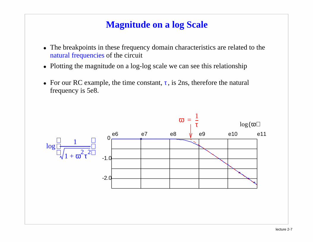
Magnitude on a log Scale

• The breakpoints in these frequency domain characteristics are related to the natural frequencies of the circuit

• Plotting the magnitude on a log-log scale we can see this relationship

1

1 ω2τ2+

--------------------------

log

ω 1τ---=

• For our RC example, the time constant, , is 2ns, therefore the natural frequency is 5e8.

τ

e6 e7 e8 e9 e10 e11

-2.0

-1.0

0

ω( )log

lecture 2-8

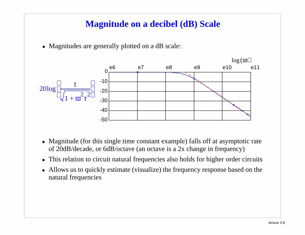
Magnitude on a decibel (dB) Scale

• Magnitudes are generally plotted on a dB scale:

201

1 ω2τ2+

--------------------------

log

• Magnitude (for this single time constant example) falls off at asymptotic rate of 20dB/decade, or 6dB/octave (an octave is a 2x change in frequency)

• This relation to circuit natural frequencies also holds for higher order circuits

• Allows us to quickly estimate (visualize) the frequency response based on the natural frequencies

e6 e7 e8 e9 e10 e11

-50

-40

-30

-20

-10

0

ω( )log

lecture 2-9

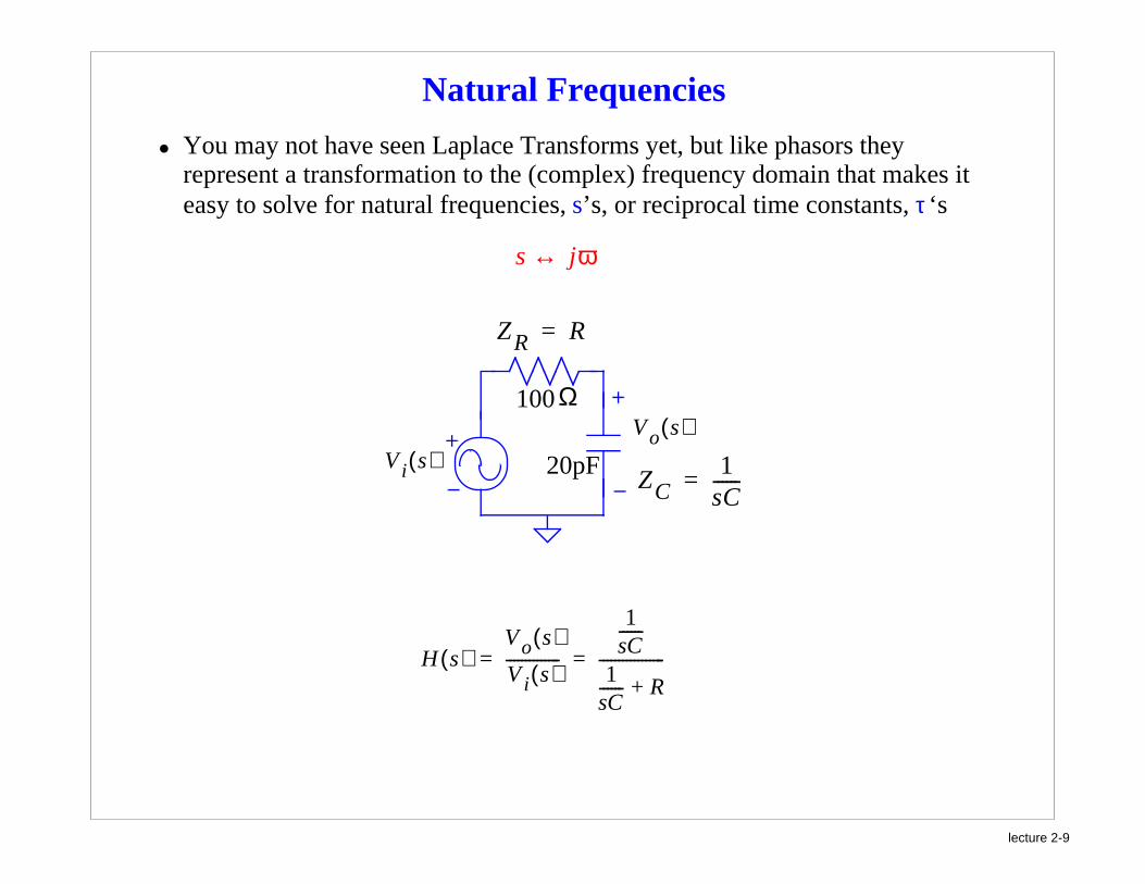
Natural Frequencies

• You may not have seen Laplace Transforms yet, but like phasors they represent a transformation to the (complex) frequency domain that makes it easy to solve for natural frequencies, s’s, or reciprocal time constants, ‘sτ

100

20pFV i s( )Vo s( )

s jω↔

H s( )Vo s( )V i s( )--------------

1sC------

1sC------ R+-----------------= =

ZC1

sC------=

ZR R=

Ω

lecture 2-10

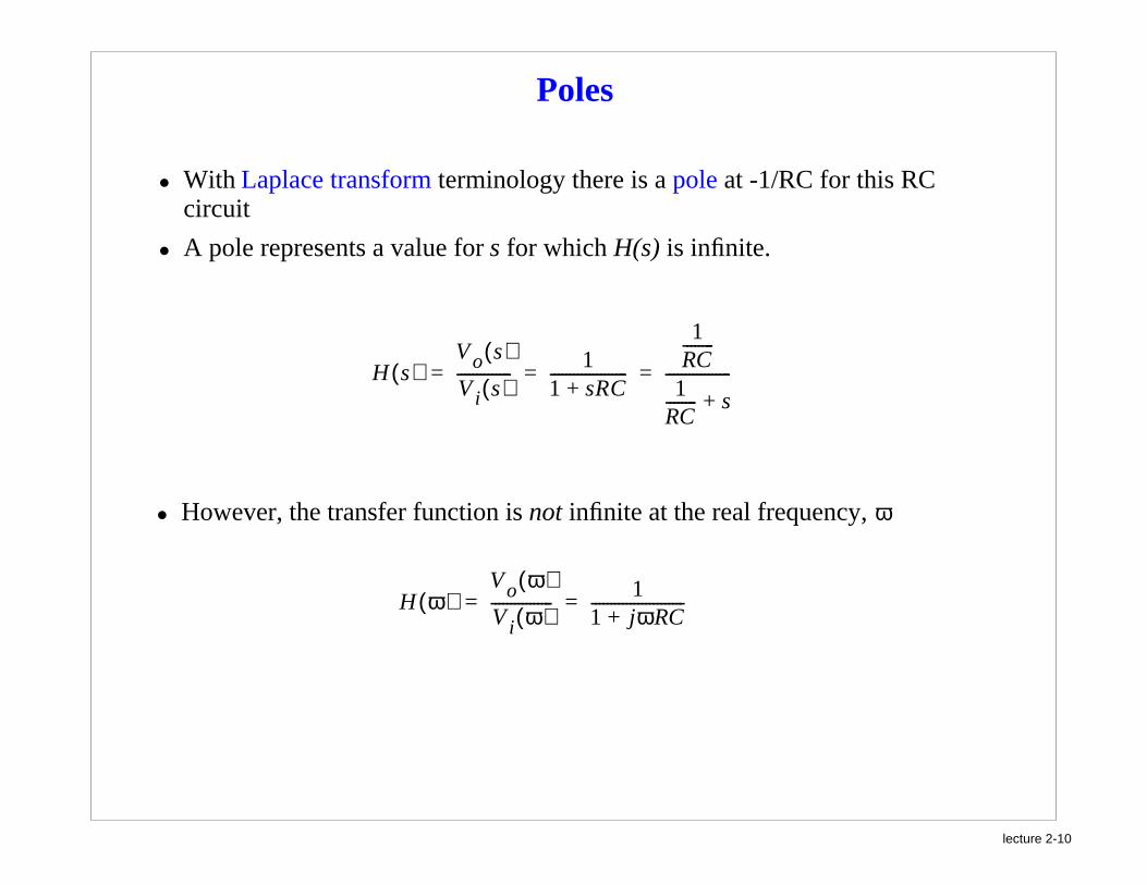
Poles

• With Laplace transform terminology there is a pole at -1/RC for this RC circuit

• A pole represents a value for s for which H(s) is infinite.

H s( )Vo s( )V i s( )--------------

11 sRC+--------------------

1RC--------

1RC-------- s+-----------------= = =

• However, the transfer function is not infinite at the real frequency, ω

H ω( )Vo ω( )V i ω( )----------------

11 jωRC+------------------------= =

lecture 2-11

Poles and Natural Frequencies

• It is important to note that naturual frequencies and time constants have positive magnitude, while poles are negative (negative real parts for RLC)

H s( )Vo s( )V i s( )--------------

11 sRC+--------------------

1

1 sp---+

-------------= = =

• p is equal to 1/RC and can be thought of as the natural frequency

• The pole which makes H(s) infinite, however, is s=-p

• We know that if we solved for the time domain response, that the s term in the assumed solution form would have to be a negative value:

Aest

lecture 2-12

Bode Plot

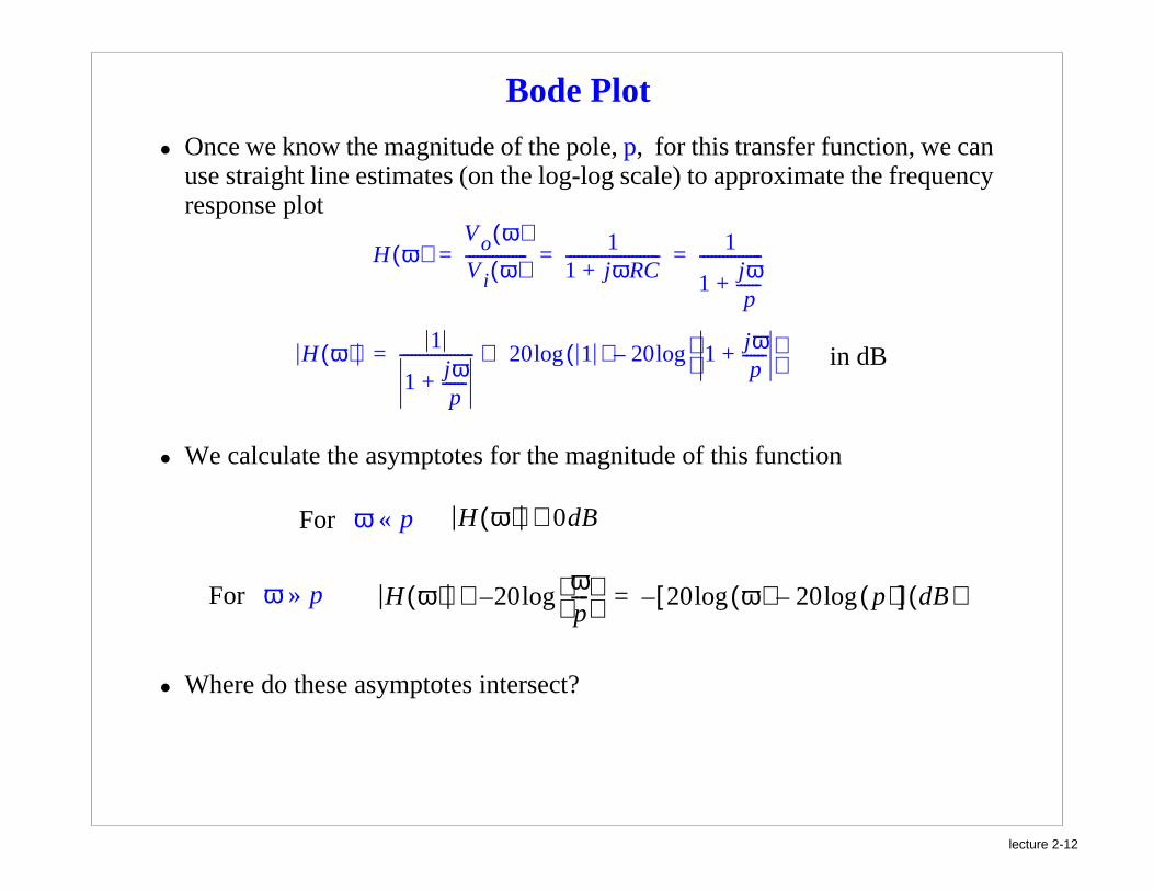
• Once we know the magnitude of the pole, p, for this transfer function, we can use straight line estimates (on the log-log scale) to approximate the frequency response plot

H ω( )Vo ω( )V i ω( )---------------- 1

1 jωRC+------------------------ 1

1jωp

------+----------------= = =

• We calculate the asymptotes for the magnitude of this function

H ω( ) 1

1 jωp

------+------------------- 20 1( ) 20 1 jω

p------+

log–log⇒=

For ω p« H ω( ) 0dB≅

For ω p» H ω( ) 20–ωp----

log≅ 20 ω( ) 20 p( )log–log[ ] dB( )–=

• Where do these asymptotes intersect?

in dB

lecture 2-13

Bode Plot

• With frequency plotted on a log scale, we can quickly sketch the asymptotes

• The maximum error at the breakpoint in the curve is known to be 3dB

-100dB

-80dB

-60dB

-40dB

-20dB

0dB

lecture 2-14

Bode Plot: Phase

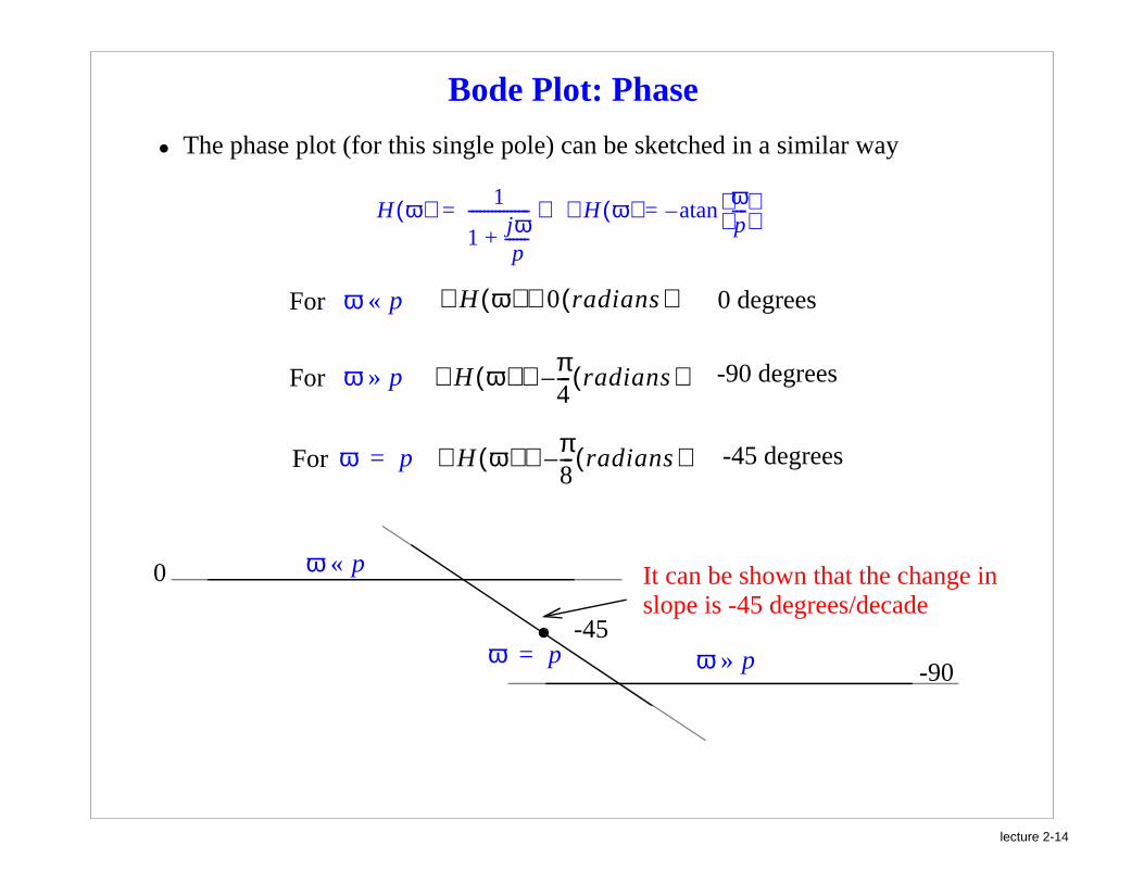
• The phase plot (for this single pole) can be sketched in a similar way

For ω p« H∠ ω( ) 0 radians( )≅

For ω p»

H ω( ) 1

1 jωp

------+---------------- H∠ ω( ) ω

p----

atan–=⇒=

H∠ ω( ) π4---– radians( )≅

For ω p= H∠ ω( ) π8---– radians( )≅

0 degrees

-90 degrees

-45 degrees

ω p«0

ω p» -90ω p=

-45

It can be shown that the change inslope is -45 degrees/decade

lecture 2-15

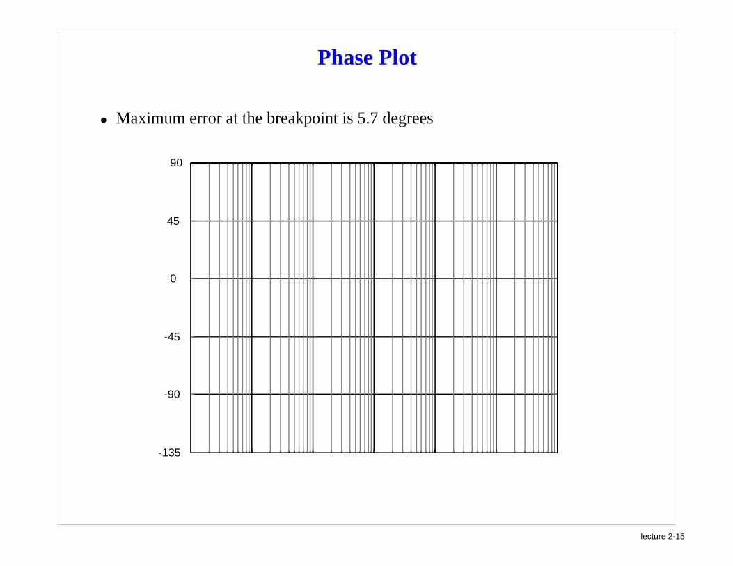
Phase Plot

• Maximum error at the breakpoint is 5.7 degrees

-135

-90

-45

0

45

90

lecture 2-16

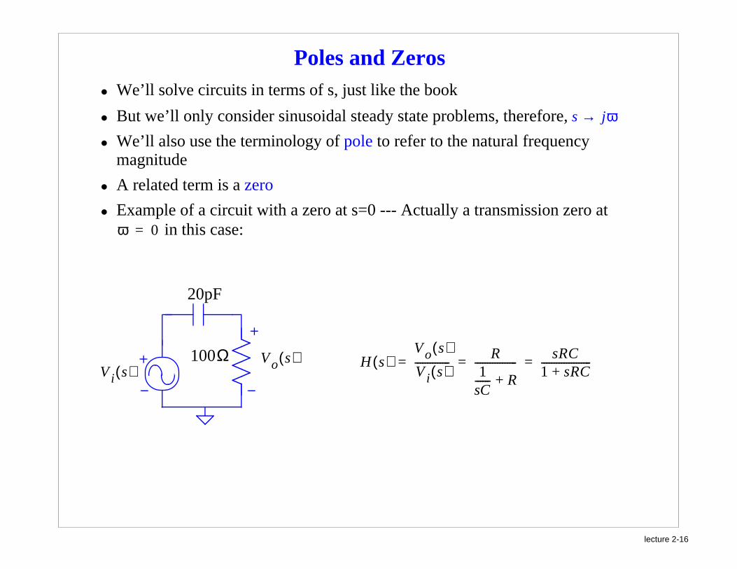
Poles and Zeros• We’ll solve circuits in terms of s, just like the book

• But we’ll only consider sinusoidal steady state problems, therefore,

• We’ll also use the terminology of pole to refer to the natural frequency magnitude

• A related term is a zero

• Example of a circuit with a zero at s=0 --- Actually a transmission zero at in this case:

s jω→

ω 0=

100

20pF

V i s( )Vo s( )Ω H s( )

Vo s( )V i s( )--------------

R1

sC------ R+-----------------

sRC1 sRC+--------------------= = =

lecture 2-17

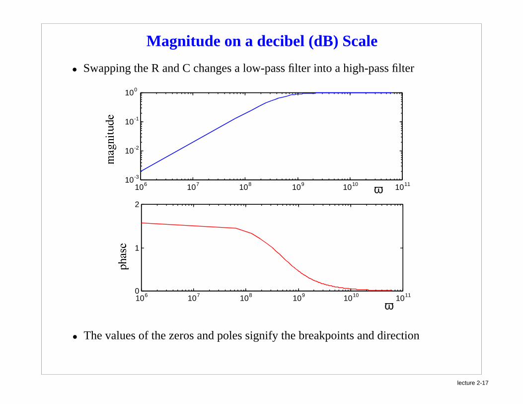
Magnitude on a decibel (dB) Scale

• Swapping the R and C changes a low-pass filter into a high-pass filter

106 107 108 109 1010 101110-3

10-2

10-1

100

106 107 108 109 1010 10110

1

2

ω

ω

• The values of the zeros and poles signify the breakpoints and direction

lecture 2-18

Bode Plot

• Once we know the pole and zero values we can apply a Bode approximation

H ω( )Vo ω( )V i ω( )---------------- jωRC

1 jωRC+------------------------

jωp----

1jωp

------+----------------= = =

• Pole term is the same as before

• Zero term is 0dB at breakpoint, and increasing at a rate of 20dB/decade otherwise

• Note that zeros create asymptotes that are increasing with frequency, while poles create asymptotes that are decreasing with frequency

• We add all of the asymptotes together to get the overall response

H ω( )jωp----

1 jωp

------+------------------- 20 j

ωp----

20 1 jωp

------+ log–log⇒=

lecture 2-19

Bode Plot

• For each term in the transfer function expression:

1. Find the direction and slope of the asymptote

2. Find one point through which the asymptote passes

-80dB

-40dB

-20dB

0dB

20dB

40dB

lecture 2-20

Poles and Zeros of Larger Circuits

• Bode plots can be used for higher-order circuits too

• But higher order circuits will have more poles and zeros, and transfer functions of the form:

• We would expect that there will always be more finite poles than zeros, why?

• What does the K-term represent?

H ω( ) K

1 jωz1------+

1 jωz2------+

… 1 jωzm------+

1jωp1------+

1jωp2------+

… 1jωpn------+

-------------------------------------------------------------------------=

lecture 2-21

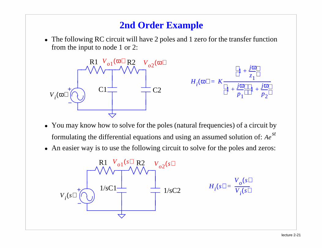
2nd Order Example• The following RC circuit will have 2 poles and 1 zero for the transfer function

from the input to node 1 or 2:

R1

V i ω( )

Vo2 ω( )

H i ω( ) K

1 jωz1------+

1jωp1------+

1jωp2------+

--------------------------------------------=

C1 C2

R2Vo1 ω( )

• You may know how to solve for the poles (natural frequencies) of a circuit by

formulating the differential equations and using an assumed solution of:

• An easier way is to use the following circuit to solve for the poles and zeros:

Aest

R1

V i s( )

Vo2 s( )

1/sC1

R2Vo1 s( )

1/sC2H i s( )

Vo s( )V i s( )--------------=

lecture 2-22

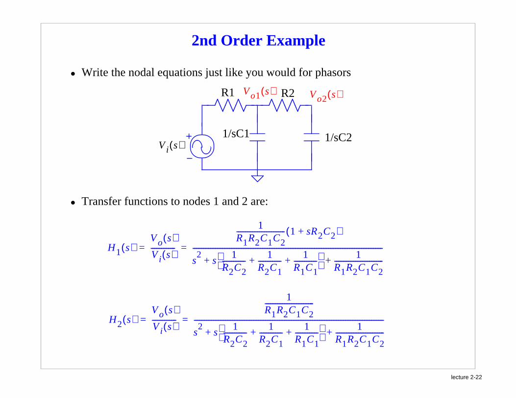
2nd Order Example

• Write the nodal equations just like you would for phasors

H1 s( )Vo s( )V i s( )--------------

1R1R2C1C2---------------------------- 1 sR2C2+( )

s2

s1

R2C2-------------

1R2C1-------------

1R1C1-------------+ +

1R1R2C1C2----------------------------+ +

-------------------------------------------------------------------------------------------------------------= =

R1

V i s( )

Vo2 s( )

1/sC1

R2Vo1 s( )

1/sC2

• Transfer functions to nodes 1 and 2 are:

H2 s( )Vo s( )V i s( )--------------

1R1R2C1C2----------------------------

s2

s 1R2C2------------- 1

R2C1------------- 1

R1C1-------------+ +

1R1R2C1C2----------------------------+ +

-------------------------------------------------------------------------------------------------------------= =

lecture 2-23

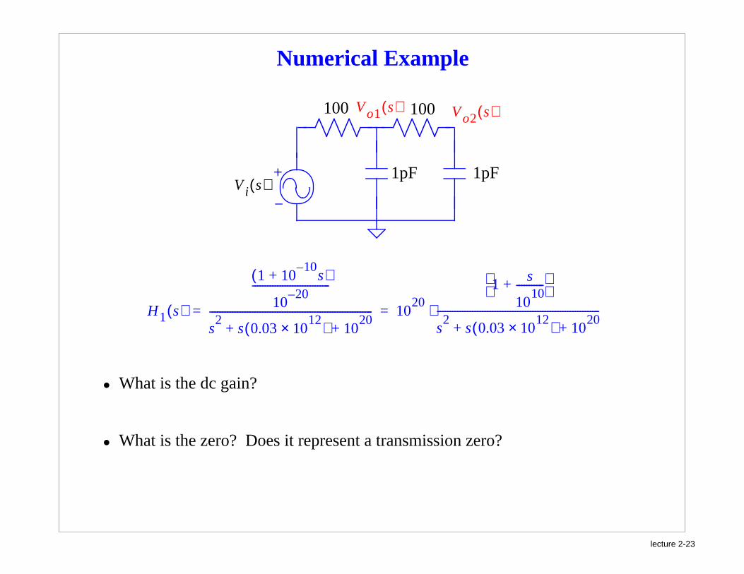
Numerical Example

H1 s( )

1 1010–

s+( )

1020–

-------------------------------

s2

s 0.03 1012×( ) 10

20+ +

----------------------------------------------------------------- 1020

1 s

1010

-----------+

s2

s 0.03 1012×( ) 10

20+ +

-----------------------------------------------------------------⋅= =

• What is the dc gain?

• What is the zero? Does it represent a transmission zero?

V i s( )

Vo2 s( )Vo1 s( )100

1pF

100

1pF

lecture 2-24

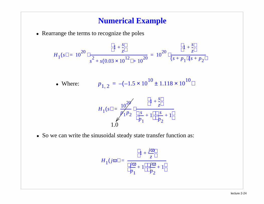
Numerical Example

• Rearrange the terms to recognize the poles

H1 s( ) 1020

1sz--+

s2

s 0.03 1012×( ) 10

20+ +

-----------------------------------------------------------------⋅ 1020

1sz--+

s p1+( ) s p2+( )----------------------------------------⋅= =

p1 2, 1.5 1010

1.118 1010×±×–( )–=

H1 s( ) 1020

p1 p2------------

1sz--+

sp1------ 1+

sp2------ 1+

-------------------------------------------⋅=

• Where:

• So we can write the sinusoidal steady state transfer function as:

H1 jω( )1

jωz

------+

jωp1------ 1+

jωp2------ 1+

--------------------------------------------=

1.0

lecture 2-25

Numerical Example

• Transfer function can be expressed as the product of the pole and zero terms:

H1 jω( )1 jω

z------+

jωp1------ 1+

jωp2------ 1+

-------------------------------------------- 1

jωz

------+ 1

jωp1------ 1+

--------------------- 1

jωp2------ 1+

---------------------⋅ ⋅= =

• If we measure the magnitude in dB, then all of the terms can be separated:

H1 jω( )dB

20 1 jωz

------+ 1

jωp1------ 1+

---------------------

1jωp2------ 1+

---------------------⋅ ⋅log= =

20 1 jωz

------+ 20

1jωp1------ 1+

--------------------- 20

1jωp2------ 1+

---------------------log+log+log

lecture 2-26

Bode Plot

• Add the asymptotes for each of the individual pole and zero contributions

-80dB

-60dB

-40dB

-20dB

0dB

20dB

lecture 2-27

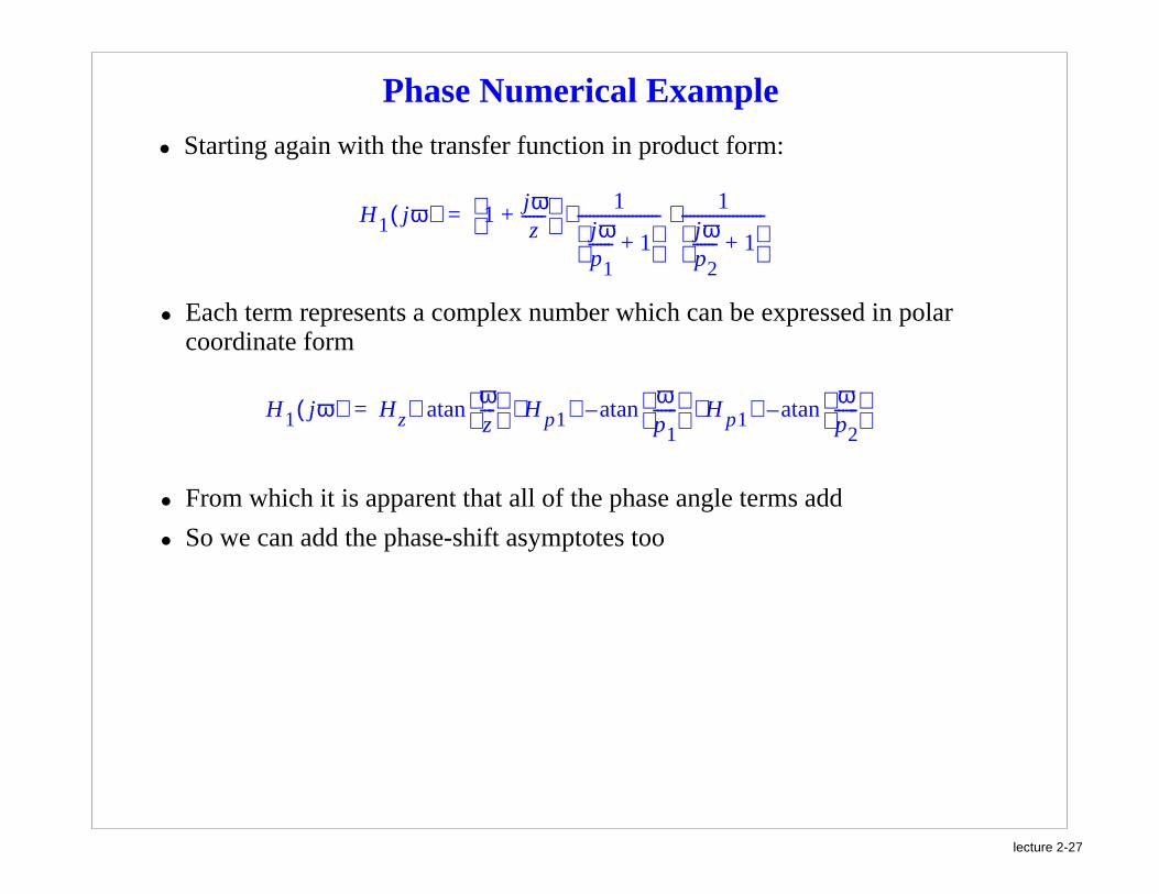
Phase Numerical Example

• Starting again with the transfer function in product form:

H1 jω( ) 1 jωz

------+ 1

jωp1------ 1+

---------------------

1jωp2------ 1+

---------------------⋅ ⋅=

• Each term represents a complex number which can be expressed in polar coordinate form

H1 jω( ) Hzωz----

atan∠ H p1ωp1------

atan–∠ H p1ωp2------

atan–∠⋅ ⋅=

• From which it is apparent that all of the phase angle terms add

• So we can add the phase-shift asymptotes too

lecture 2-28

Phase Plot

-135

-90

-45

0

45

90

lecture 2-29

Zeros at Node 2

• The zero at node 1 is 1/R2C2, but the response at node 2 does not have any finite zeros --- does this make sense?

H2 jω( ) 1jωp1------ 1+

jωp2------ 1+

--------------------------------------------=

R1

V i s( )

Vo2 s( )

1/sC1

R2Vo1 s( )

1/sC2

lecture 2-30

Bode Plot

-100dB

-80dB

-60dB

-40dB

-20dB

0dB

• The transfer functions share the same two poles, their responses are different due to the zero

lecture 2-31

Phase Plot

-135

-90

-45

0

45

90