frequency and damping characteristics of … as a generator connects to a large network system with...

Frequency and Damping Characteristics of Generators in PowerSystems

Xiaolan Zou

Thesis submitted to the Faculty of theVirginia Polytechnic Institute and State University

in partial fulfillment of the requirements for the degree of

Master of Sciencein

Electrical Engineering

Jaime De La Ree Lopez, ChairVirgilio A. Centeno

Vassilis KekatosSteve C. Southward

Decenber 6, 2017Blacksburg, Virginia

Keywords: inertia constant, inter-area mode, damping, dynamic system, local-area mode,oscillation frequency, Prony Analysis.

Copyright 2017, Xiaolan Zou

Frequency and Damping Characteristics of Generators in Power Systems

Xiaolan Zou

Abstract

A power system stability is essential for maintaining the power system oscillation fre-

quency within a small and acceptable interval around its nominal frequency. Hence, it is

necessary to study and control the frequency for stable operation of a power system by

knowing the characteristics within a power system. One approach is to understand the ef-

fectiveness of frequency and damping characteristics of generators in power systems. Hence,

the simulation analysis of IEEE 118-bus power system is used for this study. The analysis

includes theoretical analysis with a mathematical approach and simulation studies of swing

equation to determine the characteristics of damped single-machine infinite bus, which is

represented as a generator connects to a large network system with a small signal distur-

bance by line losses. Additionally, mathematical derivation of Prony analysis is presented in

order to estimate the frequency and damping ratio of the simulation results. In the end, the

results demonstrate that the frequency and damping characteristics of generators are highly

dependent on the system inertia constant. Therefore, the higher inertia constant is a critical

factor to ensure the system is more stable.

Frequency and Damping Characteristics of Generators in Power Systems

Xiaolan Zou

Abstract (General Audience)

A power system’s stability is dependent on maintaining the oscillation frequency within

a small and acceptable variance of its normal frequency. In order to control the frequency

for the stable operation of a power system, it is necessary to study the characteristics within

a power system.

One approach is to study the effectiveness of frequency and damping characteristics of

generators in power systems. For this study, the simulation analysis of the IEEE 118-bus

power system will be used. This includes a mathematical approach and simulation studies of

swing equation. These will determine the characteristics of damped single-machine infinite

bus. This is represented as a generator connected to a large network system with a small

signal disturbance caused by line losses. Additionally, the mathematical basis of Prony

analysis is presented in order to estimate the frequency and damping ratio of the simulation

results.

In the end, the results demonstrate that the frequency and damping characteristics of

generators are highly dependent on the system inertia constant. Therefore, a high inertia

constant is critical to the stability of the system.

Dedication

To My Parents: Changyin Zou and Ruiqin Lin

iv

Acknowledgments

I want to thank my academic advisor, Dr. De La Ree, for his knowledge, counseling,

and support throughout my undergraduate and graduate school years. Dr. Dee La Ree is

the one who opened my eyes to the world of power system in his undergraduate course, Intro

to Power System. His wisdom and passion to the power system encouraged me to pursue the

power system field. I would also like to thank the other committee members for all of their

guidance and support throughout my graduate school years: Dr. Centeno, Dr. Kekatos, and

Dr. Southward. It is my pleasure to work with all the committees for such a knowledgeable

thesis under their help and guidance.

My appreciation also goes to my labmates in the Power Lab. Thank you for your

support, kindness, and friendship during all these years. It is a great joy to know each of you

and many lifelong friendships were developed by working hard together to conquer different

challenges. I have learned a lot about the power system field from many of you. Thank you

for your help and encouragement.

To all my family and friends, I would not be where I am today without all of your love

and support no matter under what circumstance. Thank you for always being there for me.

I will always remember and be grateful for each one of you. I will always be there and be

supportive for all of you if you need me.

v

Contents

Dedication iv

Acknowledgments v

Contents vi

List of Figures viii

List of Tables x

1 Introduction 1

1.1 Literature Review . . . . . . . . . . . . . . . . . . . . . . . . . . . . . . . . . 2

1.2 Outline of this Thesis . . . . . . . . . . . . . . . . . . . . . . . . . . . . . . . 3

2 Characteristic Analysis of Generators through Second Order model of Ma-chine in Power System 4

2.1 Classical Model Definitions of Generators . . . . . . . . . . . . . . . . . . . . 5

2.2 Equivalent Swing Equation for A Large Network System . . . . . . . . . . . 6

2.2.1 Equivalent Inertia of Coherent Machines in Power System . . . . . . 11

2.2.2 Equivalent Inertia of Non-Coherent Machines in Power System . . . . 12

3 Prony Analysis 16

3.1 Analytical Approach . . . . . . . . . . . . . . . . . . . . . . . . . . . . . . . 16

4 Dynamic Simulation Test with IEEE-118 Bus in PSS/E 22

vi

4.1 Develop A Proper IEEE 118-bus Model in PSS/E for Analysis . . . . . . . . 23

4.1.1 Machine Model . . . . . . . . . . . . . . . . . . . . . . . . . . . . . . 25

4.1.2 Create an Network Matrix A to Avoid Island Power System . . . . . 26

4.1.3 Define Proper Disconnecting Line Events for Dynamic Simulation . . 28

4.2 Case Study for Dynamic Simulation . . . . . . . . . . . . . . . . . . . . . . . 30

4.2.1 Case Study for Damping Characteristics of Generators between Local-Area Oscillation and Inter-Area Oscillation . . . . . . . . . . . . . . . 32

4.2.2 Case Study for Frequency Characteristic of Generators under area control 37

5 Conclusion and Future Work 48

5.1 Conclusion . . . . . . . . . . . . . . . . . . . . . . . . . . . . . . . . . . . . . 48

5.2 Future Work . . . . . . . . . . . . . . . . . . . . . . . . . . . . . . . . . . . . 49

Bibliography 51

Appendices 53

A Model of Exciter 54

B Model of Governor 56

C Bus Incidence Matrix 58

C.1 Matlab Code for Bus Incidence Matrix . . . . . . . . . . . . . . . . . . . . . 59

D 186 Branches from IEEE 118-Bus 61

E Oscillation Frequency Data for All generators with All Events Study 66

vii

List of Figures

2.1 Single Machine Infinite Bus . . . . . . . . . . . . . . . . . . . . . . . . . . . 5

2.2 Swing Curve for a Group of Generators in IEEE-118 Bus . . . . . . . . . . . 12

4.1 One-Line Diagram of IEEE 118-Bus Test System . . . . . . . . . . . . . . . 24

4.2 Incidence Matrix Part2 . . . . . . . . . . . . . . . . . . . . . . . . . . . . . . 27

4.3 Dynamic Behavior of Power for G10 After Disconnecting Branch 10 . . . . . 31

4.4 Dynamic Behavior of Power for G10 After Disconnecting First 5 Branches . 33



4.7 Dynamic Behavior of Power After Disconnecting 5 Branches in Zone 2 . . . . 35

4.8 Dynamic Behavior of Power After Disconnecting 5 Branches in Zone 3 . . . . 36

4.9 Dynamic Behavior of Power for Edge Generators in Zone Two . . . . . . . . 37

4.10 Disconnecting Zone One Transmission Line . . . . . . . . . . . . . . . . . . . 39

4.11 Trend of Disconnecting Zone One Transmission Line . . . . . . . . . . . . . . 40

4.12 Abnormal Case for Disconnecting Zone One Transmission Line . . . . . . . . 41

4.13 Disconnecting Zone Two Transmission Line . . . . . . . . . . . . . . . . . . 42

4.14 Trend of Disconnecting Zone Two Transmission Line . . . . . . . . . . . . . 43

4.15 Disconnecting Zone Three Transmission Line . . . . . . . . . . . . . . . . . . 44

4.16 Disconnecting All 142 Branches . . . . . . . . . . . . . . . . . . . . . . . . . 45

4.17 Disconnecting All 142 Branches . . . . . . . . . . . . . . . . . . . . . . . . . 46

A.1 IEEET1˙Exciter . . . . . . . . . . . . . . . . . . . . . . . . . . . . . . . . . . 54

viii

B.1 Steam˙Turbine˙Governor . . . . . . . . . . . . . . . . . . . . . . . . . . . . . 56

C.1 Incidence Matrix Part1 . . . . . . . . . . . . . . . . . . . . . . . . . . . . . . 58

C.2 Incidence Matrix Part2 . . . . . . . . . . . . . . . . . . . . . . . . . . . . . . 59

ix

List of Tables

4.1 Types of Different Synchronous Machines in Different Zones . . . . . . . . . 24

4.2 Dynamic Data Setting for GENROU . . . . . . . . . . . . . . . . . . . . . . 26

4.3 Branches Cannot be Disconnected due to Island System Problem . . . . . . 28

4.4 Seven Pairs of Transmission Lines Connected in Parallel . . . . . . . . . . . 29

4.5 Divide Branches into Three Different Zones . . . . . . . . . . . . . . . . . . . 31

4.6 Oscillation Frequency and Damping Ratio Estimation for Three Generators . 38

4.7 Description of Figures . . . . . . . . . . . . . . . . . . . . . . . . . . . . . . 44

4.8 Mean Oscillation Frequency Range in Radians for Three Zones under ThreeStudies . . . . . . . . . . . . . . . . . . . . . . . . . . . . . . . . . . . . . . . 46

4.9 Mean Oscillation Frequency Range in HZ for Three Zones under Three Studies 46

A.1 IEEE Type 1 Excitation System - IEEET1 . . . . . . . . . . . . . . . . . . . 55

B.1 Steam turbine-governor model - TGOV1 . . . . . . . . . . . . . . . . . . . . 56

D.1 186 Branches from IEEE 118-Bus . . . . . . . . . . . . . . . . . . . . . . . . 61





E.1 Mean Oscillation Frequency of Each Zone By Disconnecting Lines in Zone 1 66



x





xi

Chapter 1

Introduction

Frequency is one of the most crucial factors to determine the stability and security of

the power system. For the stable operation, the frequency should be maintained within

a very small and acceptable interval around its nominal frequency value, 50 Hz or 60Hz.

Normally, oscillation frequency of local-area modes is in the range of 0.7 to 2.0 Hz and

inter-area modes is in the range of 0.1 to 0.8 Hz [1]. In recent years, frequency related

stability problems have attracted more attention due to the rapid development of integrating

renewable energy into the grid. The contribution of system inertia constant is inherent from

the rotating synchronous generator. The overall system inertia constant will be dropped

after replacing a generator by a renewable energy source, such as solar and wind power.

Hence, it is necessary to study and control the frequency range for a stable power system

by knowing the characteristics within a power system. One approach is to understand the

frequency and damping characteristics of generators in the power system in order to build

up better background in controlling the frequency in the future study.

The perturbation of a power system can be caused by fault events such as line losses or

generator losses. The dynamic behavior of frequency deviation of a power system due to the

disturbance depends on the real power of the generator. The initial generator output power

1

2

is controlled by the system inertia constant. Therefore, it is important to understand the

relationship between frequency and the system inertia constant H and the role of system

inertia constant in the power system. In addition, the results of dynamic simulation in this

document has also determined that the location of where a transmission line is tripped is

important and directly affects the frequency and damping characteristics of generators in

the power system.

1.1 Literature Review

Problems related to frequency stability and frequency response of reducing power system-

order have been identified by many researchers for several decades. A simple two machine

system and system frequency response(SFR) were described in [2] by P. M. Anderson and

M. Mirheydar in 1990. It is very similar to the approach that is described in this document

for reducing a large network system to a single-machine infinite bus system. The mathemat-

ical approach of single-machine infinite bus system and the power system stability problem

related to small-signal stability analysis were introduced by P. Kundur in [3]. In the past

decades, many researchers have worked on power system frequency regulation in [2]-[5] by

inroducing renewable generations in the power system. Therefore, the frequency issues have

been re-addressed under new paradigm in [6] to analyze the load-damping characteristic in

power system frequency regulation. Even though much research has been done to find the

effect on the system frequency due to perturbation of the power system, generator losses or

load shredding in [7], only a small portion of this research focuses on the actual frequency

and damping characteristics of generators in power systems. It is necessary to analyze the

frequency characteristics of generators under the stable operation of power systems to help

us to investigate the relationship between dynamic behavior of generators and the system

3

inertia constant.

1.2 Outline of this Thesis

This thesis documents the simulation analysis of the generator output power in IEEE

118-bus power system, which determines the frequency and damping characteristics of gen-

erators in power systems. Chapter 2 describes the detailed processes of a mathematical

approach through swing equations to determine that single-machine infinite bus is an ap-

proximate representation of a real power system; the system is a second order model system.

It also concludes the relationship between frequency and inertia. Chapter 3 provides the

mathematical method to derive Prony analysis, along with the considerations for applying

Prony analysis to estimate the frequency and damping ratio of the transient waveforms in

Chapter 4. Chapter 4 provides the results of all the dynamic simulation with detailed analy-

sis included. In addition, a proper IEEE 118-bus power system is developed with description

of detailed model information. Chapter 5 is the summary of the thesis. It also includes the

conclusion of all the simulation results from Chapter 4 and future work is presented. Next

is the list of references. In the end, there is a set of appendices. The appendices provide

models of exciters and governors for the power system and useful information related to the

simulations.

Chapter 2

Characteristic Analysis of Generatorsthrough Second Order model ofMachine in Power System

Modern power systems are very complex and nonlinear. It is difficult to analyze a large

power system with numerous machines, lines and loads. It is also difficult to determine

the results of any impact from any disturbance, such as transmission system faults, load

change, loss of generators and loss of lines or tripping lines. Therefore, when the behavior of

one synchronous machine is studied in a very large system, the big system can be reduced

to an equivalent single-machine against an infinite bus for the rest of the system, which is

also described as single-machine infinite bus(SMIB) in power systems. The single-machine

infinite bus power system is an approximate representation of a real power system, where a

power plant with a generator or a group of generators are connected by transmission lines

to a very large power network. In this research, the focus will be on a generator that is

connected to a large power network through a transmission line to study the oscillation

frequency of the generators output power of the power system in dymnamic analysis. The

one-line diagram of the single machine infinite bus system is illustrated in Figure 2.1, which

describes the generator on the left delivers power to a large network. The capacity of the

4

5

generator is much smaller compared to the capacity of the large network on the right. The

operation of the large network is not affected at all by any change made by the generator

on the left. As a result, the large network system is able to be repredented an infinite bus

refer to the point of view of the left hand side generator. The infinite bus is considered as a

generator with infinite inertia, fixed voltage and zero impedance [3].

Figure 2.1: Single Machine Infinite Bus

2.1 Classical Model Definitions of Generators

The classical model is the simplest model of all the synchronous machine models. It

can also be called the constant voltage behind the transient reactance model [8]. In order

to achieve the idea of the classical model, the dynamics of exciter, damper windings, rotor

windings, dynamic of turbines, and turbine speed governor need to be neglected. There-

fore, the assumption of the classical model of a synchronous generator can be represented

mathematically below [3]:

1. The induced voltage of the generator stator has to be constant all the time by control-

ling the field current to be constant and to ignore the dynamic of exciter.

2. The effects of damper windings, which is shown on the rotor of the synchronous gen-

erator, is neglected.

6

3. The input mechanical power to the generator is assumed to be constant during the

simulation.

2.2 Equivalent Swing Equation for A Large Network

System

The swing equation describes the relative motion that is caused by rotor deceleration

or acceleration with respect to the motion of the rotor of a synchronous machine during the

disturbance. The prime mover from synchronous generators converts mechanical energy to

electrical energy based on magnetic coupling. The accelerating torque is produced by the

moment of inertia from the rotating rotor and its angular acceleration [9]. The rotational

dynamic swing equation can be represented below:

J · ∂2θm∂t2

= Ta = Tm − Te N ·m (2.1)

Where,

• J is the moment of inertia for the rotating masses in kg-m2;

• θm is the angular displacement of the rotor respect to a stationary axis in radians;

• t is the time in s;

• Tm is net mechanical torque produced by prime mover in N-m;

• Te is net electrical torque or load torque in N-m;

• Ta is net accelerating torque in N-m.

7

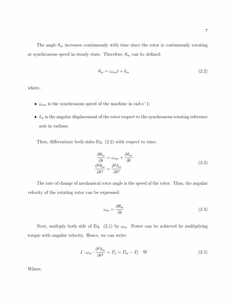
The angle θm increases continuously with time since the rotor is continuously rotating

at synchronous speed in steady state. Therefore, θm can be defined:

θm = ωsmt+ δm (2.2)

where,

• ωsm is the synchronous speed of the machine in rad·s−1;

• δm is the angular displacement of the rotor respect to the synchronous rotating reference

axis in radians.

Then, differentiate both sides Eq. (2.2) with respect to time:

∂θm∂t

= ωsm +∂δm∂t

∂2θm∂t2

=∂2δm∂t2

(2.3)

The rate of change of mechanical rotor angle is the speed of the rotor. Thus, the angular

velocity of the rotating rotor can be expressed:

ωm =∂θm∂t

(2.4)

Next, multiply both side of Eq. (2.1) by ωm. Power can be achieved by multiplying

torque with angular velocity. Hence, we can write:

J · ωm ·∂2δm∂t2

= Pa = Pm − Pe W (2.5)

Where,

8

• Pm is the mechanical input power in watts;

• Pe is the electrical output power in watts;

• Pa is the accelerating power refers to the power difference between mechanical power

and electrical power in watts.

Then, the new parameter M, which is called inertia constant of the machine, is denoted

to be J·s·radˆ-1 since M is the product of J and ωm. Then, the swing equation can be

rewritten below:

M∂2δm∂t2

= Pa = Pm − Pe (2.6)

M is assumed to be constant because ωm is only slightly off from synchronous speed ωms

when the synchronous machine is stable. M can also be obtained from:

M =2H

ωsm· Smach MJ/mech rad (2.7)

Where H is known as machine inertia constant in second, or as rotational inertia, and

is defined as the equation below:

H =Stored kinetic energy in MJ at synchronous speed

Machine rating in MVA(2.8)

The mathematical expression for H is described as:

H =12Jω2

sm

Smach=

12Mωsm

Smach[MJ/MV A] (2.9)

9

By combining both Eq. (2.6) and Eq. (2.7), the swing equation can be rearranged with

respect to rotating inertia H:

2H

ωms

∂2δm∂t2

=Pa

Smach=Pm − PeSmach

(2.10)

and

2H

ωs· ∂

2δo∂t2

= Pa = Pm − Pe p.u. (2.11)

Where,

• δo is the rotor angle of the synchronous machine in radians

• ωs is the synchronous speed of the machine in radians per second

• H is machine inertia constant in second

The machine angular speed is equal to the synchronous speed in the steady state. Hence,

we change ωms to ωs in Eq. (2.11). When the damping constantKd is introduced to the power

system due to the friction from the prime mover, damping windings, or any other damping

sources, the swing equation can be obtained below to express the dynamic behavior of a

synchronous machine:

2H

ωs· ∂

2δo∂t2

= Pa = Pm − Pe −Kd∂δo∂t

(2.12)

Next, when consider the small signal disturbance to the power system, a small incre-

mental displacement angle δ∆ would be introduced to the rotor angle δo, which is under

10

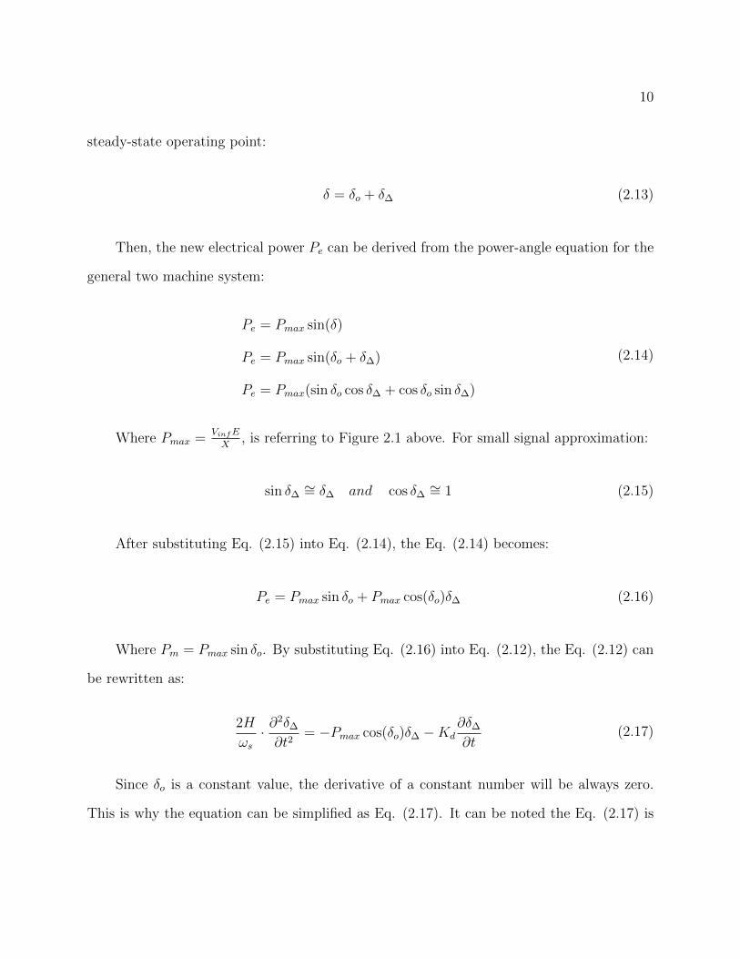
steady-state operating point:

δ = δo + δ∆ (2.13)

Then, the new electrical power Pe can be derived from the power-angle equation for the

general two machine system:

Pe = Pmax sin(δ)

Pe = Pmax sin(δo + δ∆)

Pe = Pmax(sin δo cos δ∆ + cos δo sin δ∆)

(2.14)

Where Pmax =VinfE

X, is referring to Figure 2.1 above. For small signal approximation:

sin δ∆∼= δ∆ and cos δ∆

∼= 1 (2.15)

After substituting Eq. (2.15) into Eq. (2.14), the Eq. (2.14) becomes:

Pe = Pmax sin δo + Pmax cos(δo)δ∆ (2.16)

Where Pm = Pmax sin δo. By substituting Eq. (2.16) into Eq. (2.12), the Eq. (2.12) can

be rewritten as:

2H

ωs· ∂

2δ∆

∂t2= −Pmax cos(δo)δ∆ −Kd

∂δ∆

∂t(2.17)

Since δo is a constant value, the derivative of a constant number will be always zero.

This is why the equation can be simplified as Eq. (2.17). It can be noted the Eq. (2.17) is

11

a second order differential equation after rearrangement of equation:

2H

ωs· ∂

2δ∆

∂t2+Kd

∂δ∆

∂t+ Pmax cos(δo)δ∆ = 0 (2.18)

It can also be noted that the equation is in second order standard form. Therefore, the

power system dynamic characteristics for one machine and infinite bus with second order

model by the expression for δ∆ as a function of time can be studied. The approximated

angular frequency and corresponding damping ratio for the machine can be derived:

ωn =

√ωs · Pmax · cos δo

2H(2.19)

ζ =1

2Kd

√ωs

2H · Pmax · cos δo(2.20)

2.2.1 Equivalent Inertia of Coherent Machines in Power System

The two machines are defined as coherence machines when two machines swing together

with their transient waveforms under a fault or multiple faults occur within an area, and their

angular difference is constant within a certain tolerance over a certain time interval [11]. The

characteristic of generators swinging together is illustrated in Fig. 2.2 as an example, which

displays the swing curves for a coherent group of three generators, when a fault occurs in the

IEEE-118 bus system. The swing equations of coherent machines can be combined to reduce

the number of swing equations for analysis in stability study for a large system[9]. Therefore,

the overall system equivalent rotating inertia can be estimated by summing rotating inertia

H of each generator together.

12

Figure 2.2: Swing Curve for a Group of Generators in IEEE-118 Bus

2.2.2 Equivalent Inertia of Non-Coherent Machines in Power Sys-

tem

Non-coherent machines are contrary to coherent machines. The two machines do not

swing together for non-coherent machines under a fault or multiple fault within an area.

This research mainly focuses on non-coherent machines dynamic behaviors. For any pair

of machines, one machine has rotor angle δ1 and another machine has rotor angle δ2. The

swing equation for each of the machine can be obtained based on Eq. (2.11):

2H1

ωs· ∂

2δ1

∂t2= Pm1 − Pe1 p.u. (2.21)

2H2

ωs· ∂

2δ2

∂t2= Pm2 − Pe2 p.u. (2.22)

13

When we subtracted Eq. (2.21) from Eq. (2.22) and divide the coefficient before second

derivative of δ, the new equation becomes:

∂2δ1

∂t2− ∂2δ2

∂t2=ωs2

(Pm1 − Pe1

H1

− Pm2 − Pe2H2

) (2.23)

Then, multiply both side with H1H2

H1+H2and rearrange the equation:

2

ωs(H1H2

H1 +H2

)∂2(δ1 − δ2)

∂t2=Pm1H2 − Pm2H1

H1 +H2

− Pe1H2 − Pe2H1

H1 +H2

(2.24)

Eq. (2.24) can be simplified further as following:

2

ωs·H12

∂2δ12

∂t2= Pm12 − Pe12 (2.25)

δ12 = δ1 − δ2 (2.26)

H12 = H1H2

H1+H2(2.27)

Pm12 = Pm1H2−Pm2H1

H1+H2(2.28)

Pe12 = Pm2H2−Pe2H1

H1+H2(2.29)

Where δ12 is the angle difference between two machines and H12 is the equivalent con-

stant inertia for two machines. Eq. (2.25) can be applied to a two-machine system when

a generator is connecting to a synchronous motor with a pure reactance in between [9].

The power, generated by the generator, is always absorbed by the motor in responding to

conversion of energy. We obtain:

Pm1 = −Pm2 = Pm (2.30)

Pe1 = −Pe2 = Pe (2.31)

14

By substituting Eq. (2.30) and Eq. (2.31) back to Eq. (2.28) and Eq. (2.29) respectively

to get Pm12 = Pm and Pe12 = Pe. Then, we can reduce the simplified combined swing

equations for two machine as follows:

2

ωs·H12

∂2δ12

∂t2= Pm − Pe (2.32)

Hence, we can conclude from Eq. (2.32) that two synchronous machine in a system can

be reduced to an equivalent of one machine against an infinite bus refer to Eq. (2.11). The

inertia constant of equivalent machine is H12 as defined in Eq. (2.27). Similarly, there is an

existing damping constant KD to the equivalent machine. Then, the swing equation can be

described as a second order differential equation for two synchronous machines under small

signal application to the power system,:

2H12

ωs· ∂

2δ12

∂t2+KD

∂δ12

∂t+ Pmax cos(δo)δ12 = 0 (2.33)

ωn =

√ωs · Pmax · cos δo

2H12

[rad/s] (2.34)

ζ =1

2KD

√ωs

2H12 · Pmax · cos δo(2.35)

Eq. (2.33) describes the dynamic behavior of an equivalent machine, which is derived

from two non-coherent synchronous machines system.

It can be concluded that the overall system oscillation frequency of the system is in-

versely proportional to the inertia constant of the overall system. The system with larger

inertia constant would be difficult to perturbed by the disturbance. On the contrary, the

system with smaller inertia constant would be more easily perturbed by the same distur-

bance. Therefore, the larger power system with larger inertia constant is more stable. The

system constant inertia is directly related to the generator output power. This document

15

emphasizes on each generator’s characterization based on analyzing the dynamic simulation

of generator power output in the dynamic system. A reduced two-machine system prob-

lem in a large network system will be studied as well. Ideally, the original swing equation

demonstrates how one machine with finite inertia swings against an infinite bus. However,

there is no infinite bus in reality. Therefore, we assume a large power system as a infinite

bus, when it connects to a generator with finite inertia. Hence, the dynamic behavior anal-

ysis of a generator is studied in a IEEE-118 bus system when a line tripping or a generator

disconnecting from the system by continuously operating the system for a certain period of

time. Chapter 4 contains a more detailed discussion.

Chapter 3

Prony Analysis

Prony Analysis is a signal analysis technique that is widely used in the area of power

systems to model damped signals. Prony Analysis is used to estimate oscillation modes by

decomposing a signal into a sum of sinusoidal components. For each component, the analysis

can directly estimate the frequency, damping ratio, and relative phase of the given signal

[14].

3.1 Analytical Approach

A set of linear differential equations can be represented as a Linear-Time Invariant (LTI)

power system dynamics for an operation point [15]:

x(t) = Ax(t) +Bu(t) (3.1)

y(t) = Cx(t) +Du(t) (3.2)

x ∈ R is the state of the system and y ∈ Rn is the output of the system. Consider the

system has the initial state x(t0) = x0 at the time t0 for the state representation of system

as shows above. If the system has homogeneous solution with input u(t) = 0 for all t or

16

17

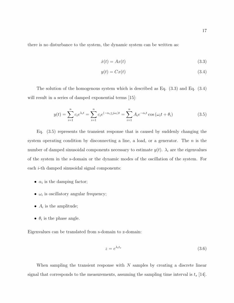
there is no disturbance to the system, the dynamic system can be written as:

x(t) = Ax(t) (3.3)

y(t) = Cx(t) (3.4)

The solution of the homogenous system which is described as Eq. (3.3) and Eq. (3.4)

will result in a series of damped exponential terms [15]:

y(t) =n∑i=1

cieλit =

n∑i=1

cie(−αi+jωi)t =

n∑i=1

Aie−αit cos (ωit+ θi) (3.5)

Eq. (3.5) represents the transient response that is caused by suddenly changing the

system operating condition by disconnecting a line, a load, or a generator. The n is the

number of damped sinusoidal components necessary to estimate y(t). λi are the eigenvalues

of the system in the s-domain or the dynamic modes of the oscillation of the system. For

each i-th damped sinusoidal signal components:

• αi is the damping factor;

• ωi is oscillatory angular frequency;

• Ai is the amplitude;

• θi is the phase angle.

Eigenvalues can be translated from s-domain to z-domain:

z = eλits (3.6)

When sampling the transient response with N samples by creating a discrete linear

signal that corresponds to the measurements, assuming the sampling time interval is ts [14].

18

This can be written as follows:

y(t) = y(kts) =n∑i=1

Bie(λits)k =

n∑i=1

Bizki for k = 1, 2, ..., N (3.7)

where,

• zi is the eigenvalues of the system in the z-domain;

• Bi is the residual of zi;

• k is the number of samples.

Eq. (3.7) can be expressed in more details by applying each ts in Eq. (3.7) to form

following equation [14]:

ZB = Y (3.8)

B1z01 + ... + Bnz

0n

B1z11 + ... + Bnz

1n

...

B1zN−11 + ... + Bnz

N−1n

=

z01 z0

2 ... z0n

z11 z1

2 ... z1n

......

...

zn−11 zn−1

2 ... zn−1n

︸︷︷︸

Z

B1

B2

...

Bn

︸︷︷︸

B

=

y(0)

y(1)

...

y(N − 1)

︸︷︷︸

Y

(3.9)

Where Z is Vandermonde matrix, which is a matrix with the terms of a geometric progression

in each row [16]. The zi is the roots of the n-th order characteristic polynomial function

and zi might be complex number as well. Then, the n-th order characteristic polynomial

equation can be formed with the coefficient ai:

zn − (a1zn−1 + a2z

n−2 + ...+ anz0) = 0 (3.10)

19

Next, construct the n-th order characteristic polynomial equation in matrix form:

[1 −a1 −a2 .. −an

]︸︷︷︸

A

zn

zn−1

zn−2

...

z0

︸︷︷︸

z

= 0 (3.11)

The A matrix can be express as a (1×N) array

[1 −a1 −a2 .. −an

]. After that,

multiply matrix A to Eq. (3.8) in both sides and apply Eq. (3.8) into the new equation. A

linear prediction model can be formulated below after minor reordering:

AY = y(n)− [a1y(n− 1) + a2y(n− 2) + ...+ any(0)]

AY = AZB

AY = [zn1 − (a1zn−11 + a2z

n−21 + ...+)anz

01 ]B1 + ...

AY = 0×B1 + 0×B2 + ...

AY = 0

y(n) = a1y(n− 1) + a2y(n− 2) + ...+ any(0)

(3.12)

20

When the time is selected arbitrarily, the signal from n step to (N − 1) step can be

applied repeatedly to form:

y(n− 1) y(n− 2) ... y(0)

y(n− 0) y(n− 1) ... y(1)

y(n+ 1) y(n− 0) ... y(2)

......

......

y(N − 2) y(N − 3) ... y(N − n− 1)

︸︷︷︸

T

a1

a2

a3

...

an

︸︷︷︸

a

=

y(n+ 0)

y(n+ 1)

y(n+ 2)

...

y(N − 1)

︸︷︷︸

b

(3.13)

where T is Toeplitz matrix, which means each descending diagonal has constant values

[17]. Eq. (3.13) can be used to solve for an unknown vector a by using pseudoinverse if

matrix T is not a square matrix. The solution of matrix a is polynomial coefficients and

calculated below:

a = inv(T ′T ) ∗ T ′b (3.14)

Furthermore, z can be found from the roots of polynomial function in Eq. (3.10) in

z-domain. Then, Vandermonde matrix Z can be formulated. The residual B are able to be

calculated since matrix Y is known measurements by applying Eq. (3.8). It is necessary to

use pseudoinverse if Z is not always a square matrix, n× n.

B = inv(Z ′Z)Z ′Y (3.15)

The eigenvalues are usually translated back to s-domain for power system application.

Then, the signal y(t) can be estimated through reconstructing y(t) based on oscillatory

angular frequency ω and damping ratio ζ. Oscillatory angular frequency is really close to

21

the imaginary part of eigenvalue in s-domain when the damping ratio is very small. The

damping ratio is defined:

ζ =α√

α2 + ω2(3.16)

For Prony Analysis, additional modes may be required to fit signal offset or noise and

the number of prediction modes n is usually smaller than the total number of samples N .

However, the reconstructed signal y(t) does not usually completely fit the original signal y(t)

in order to avoid over-fit of the signal [14]. In this case, it cannot predict too many modes

using Prony analysis.

Chapter 4

Dynamic Simulation Test withIEEE-118 Bus in PSS/E

In order to study the effect of a single-line trips on the oscillation frequencies in the power

system, the IEEE 118-bus system was used. Initially, faults were applied to the network with

the purpose of determining the coherent groups of generators within the system. As a result,

three different coherent groups were identified. Then, the dynamic simulation of single-line

trips with PSS/E was performed and the oscillations experienced by each generator in each

of the three areas was recorded. Prony analysis was applied to the samples collected of

real power output of each generator to estimate the oscillation frequencies of each signal.

In order to generalize the findings and visualize them properly, averaging and polynomial

curve fitting were performed on all the highest oscillation frequency for all the generators

with all the events in three different case studies. Three case studies are defined by dividing

the transmission lines into three groups based on which areas they are located. The branch

numbers were listed in progression from bus 1 to bus 118, refer to Table D.2. The study

demonstrates that partitioning into areas makes sense since line tripping within areas cause

larger frequency oscillations in generators within the area, and had minor effect in out-of-

area generators. Tripping of tie-lines on the other hand would affect generators from both

22

23

areas.

4.1 Develop A Proper IEEE 118-bus Model in PSS/E

for Analysis

A proper power system model is developed for 118-bus system for analyzing the fre-

quency and damping characteristics of generators in power systems. A system description

of the IEEE 118-bus modified power system follows. It has 54 synchronous machines with

IEEE type 1 excitation system model and Steam turbine-governor model. Fifteen of the

synchronous machines are motors and 20 of the synchronous machines are synchronous con-

densers, which are only used to support reactive power in the system. Furthermore, the

118-bus system also contains 118 buses, 186 transmission lines, 9 transformers, and 91 con-

stant impedance loads[18]. The total loads of the system consume 3668 MW real power and

1438 MVAr reactive power. The swing bus of 118-bus power system is bus 69. There are

three different zones in 118-bus power system. The one-line diagram of the IEEE 118-bus

test system is visualized in Figure 4.1 and was modified from its original one-line diagram

in [19] in order to match the power system that this report used for dynamic simulations.

24

Figure 4.1: One-Line Diagram of IEEE 118-Bus Test System

The different types of synchronous machines in different zones have been identified in

Table 4.1. Only the generators connect to the buses 10, 25, 26, 61, 65, 69, 87, 89, and

111, which have no loads connecting to the same bus, can be applied with swing equations,

derived from Chapter 2.

Table 4.1: Types of Different Synchronous Machines in Different Zones

Bus Number Machine Type Zone1, 6, 15, 18, 19, 32 Synchronous Compensator One4, 8, 24, 27, 113 Motor One10, 12, 25, 26, 31 Generator One

34, 36, 49, 55, 56, 62, 70, 74, 76, 77 Synchronous Compensator Two40, 42, 72, 73, 116 Motor Two

46, 49, 54, 59, 61, 65, 66, 69, 80 Generator Two85, 92, 104, 105, 110 Synchronous Compensator Three87, 89, 100, 103, 111 Generator Three90, 91, 99, 107, 112 Motor Three

25

4.1.1 Machine Model

The type of machine that is used in PSS/E for dynamic simulation for all 54 machines

is a round rotor generator model. The dynamic data setting for this model is described in

Table 4.2. All the machines have the same dynamic setting and their inertia constant H

all have the value 3.2. All the dynamic models of the exciters are IEEE Type 1 excitation

systems, which are called IEET1 in PSS/E. And all the dynamic models of governors are

steam turbine-governor models, which are called TGOV1 in PSS/E. A detailed explanation

of both exciter and governor is covered in Appendix A with both one-line diagrams and

dynamic data setting.

26

Table 4.2: Dynamic Data Setting for GENROU

Parameters GENROU Description [12]T ′do 4.8000 d-axis transient rotor time constantT ′′do 0.35000E-01 d-axis sub-transient rotor time constantT ′qo 1.50000 q-axis transient rotor time constantT ′′qo 0.7000E-01 q-axis sub-transient rotor time constantH 3.2 Inertia constantD 0 Damping factor (p.u.)Xd 1.8000 Xd-axis synchronous reactanceXq 1.750000 Xq-axis synchronous reactanceX ′d 0.30000 Xd-axis transient reactanceX ′q 0.470000 Xq-axis transient reactance

X ′′d = X ′′q 0.23000 Xd-axis sub-transient reactance, Xq-axis sub-transient reactanceXl 0.15000 stator leakage reactance

S(1.0) 0.1 saturation factor at 1.0 pu fluxS(1.2) 0.4 saturation factor at 1.2 pu flux

4.1.2 Create an Network Matrix A to Avoid Island Power System

In order to perform a small signal analysis, a transmission line with low power flow was

disconnected and simulated using PSSE. Tripping of a line should never create an island

or isolated power system due to the limitation of the numerical solution provided by the

simulation package. For a small system, it is easy to identify the island system problem

by checking on the one-line diagram. However, it is more complicated to identify the same

problem in a one-line diagram with a large network power system. Hence, a network matrix

A can be created to solve this power system problem. The form of the network matrix is

depending on the frame of reference, bus or loop [20]. In here, a bus incidence matrix A is

created. The total number of buses represent the number of columns (NBus) and the total

number of rows represent the total number of branches (NBranch). Then, the dimension of

the matrix A is NBranch×NBus, which is equal to 186×118 refer to the introduction of IEEE

27

118-bus in Chapter 3.1. The element of matrix are described as below:

• aij = 1 if the ith branch is the path that is oriented away from the jth bus.

• aij = -1 if the ith branch is the path that is oriented toward to the jth bus.

• aij = 0 if the ith branch is not in the path.

The bus incidence matrix A can be used to identify the bus or buses with a single-line

connecting them to the system. Those are the single lines that cannot be removed from the

system for the dynamic study as it will create two independent systems and the simulation

will fail. The matrix can be displayed in a GUI table as showed in Figure 4.2. The completed

matlab example code and generated matrix image for the bus incidence matrix are listed

in Appendix B. The full matrix can be viewed by scrolling through the columns or rows by

using a slider uicontrol in the GUI table.

Figure 4.2: Incidence Matrix Part2

After running the Matlab code in Appendix B, bus number 10, 73, 87, 111, 112, 116,

28

and 117 have been identified as having only one transmission line connecting to these buses.

All the line segments associated with radially connected buses cannot be disconnected as

they will result a system islanding. As a result, the system has 9 branches that cannot be

disconnected in the simulation. The detailed list of 9 branches is displayed in Table 4.3 with

the corresponding buses that will be isolated if the branch is disconnected. The detailed

connections of 186 transmission lines have been listed in Appendix D.

Table 4.3: Branches Cannot be Disconnected due to Island System Problem

Branch Number From Bus To Bus Isolated Bus12 8 9 9 and 1014 9 10 1019 12 117 117108 68 116 116116 71 73 73137 85 86 86 and 87140 86 87 87175 110 111 111176 110 112 112

4.1.3 Define Proper Disconnecting Line Events for Dynamic Sim-

ulation

In addition to the transmission lines which involve a bus break up into an island power

system problem, there are three more situations that need to be considered in order to

prepare the case study by disconnecting proper transmission lines for dynamic simulation

with small signal disturbance.

• First, if two parallel transmission lines are connected between two buses, it is redundant

work to disconnect each of parallel lines for studying the dynamic systems separately.

This is because the behavior of the system for each event will be the same for all

29

the parallel transmission lines. The 118-bus system has 7 pairs of transmission lines

connecting in parallel as shown in Table 4.4. Therefore, there will be only one trans-

mission line that is disconnected from each pair of parallel transmission lines during

the case study for dynamic simulation.

• Second, some buses are connected by two-winding transformers, which is listed at

Table D.1 in Appendix D from branch 178 to branch 186. These nine branches will

also be excluded from the dynamic simulation study.

• Finally, all the transmission lines that transfer more than 100 MW real power between

two buses will be excluded from the dynamic simulation case study in this research

with exception of the tie-lines.

As a result, there are only 142 branches left for the dynamic study, which consists of

disconnecting one branch at a time to analyze the frequency characteristic of each generator

of the power system with small signal disturbance. All 142 branches have been listed in

Table D.2 in Appendix D.

Table 4.4: Seven Pairs of Transmission Lines Connected in Parallel

From Bus To Bus42 4949 5449 6656 5977 8089 9089 92

30

4.2 Case Study for Dynamic Simulation

All the case studies for dynamic simulation will be run in PSS/E through Python code.

For each event, there is only one transmission line that is disconnected from the system.

Then, the data for dynamic behavior of rotor angles, power, field voltage, bus voltage, and

frequency deviation of each generator can be extracted from PSS/E. The total simulation

time is 15s for each event and the time step used in the simulation run was equal to a half

cycle for a 60-Hz system. Therefore, each signal has 1806 points. The oscillation is always

returning back to steady state after 10s for most of the simulation signals, so the study will

only analyze the results of the initial 10s of simulation, which means 1205 data points in

total. For each event, there are 54 dynamic simulation waveforms of output power of each

individual generator. All the data will be processed and all the waveforms generated. Not

all of data will be shown in this report.

The dynamic behavior of the power of each individual generator will be analyzed to de-

termine the frequency and damping associated with each generator for each event. Dynamic

behavior of power for generator 10 by disconnecting branch 10, which is from bus 7 to bus

12 refer to Table D.2, is illustrated in Figure 4.3. The output power in per unit produced by

each generator is displayed in the y-axis, while the x-axis represents the simulation time in

seconds. In the first 0.5 second of the simulation, the power system is operating without any

disturbance. The 0.5s simulation is done to check if the system is under steady state prior

to the event. Following the loss of a transmission line, the change of frequency and response

of the generator output is evaluated. The generator output power is dominantly influenced

by machine inertia constant with fast response soon after the disturbance. Meanwhile, the

governor has a minor effect at this point because governor and exciter has a relatively long

time constant to respond.

31

0 1 2 3 4 5 6 7 8 9 10

time in s

4.492

4.494

4.496

4.498

4.5

4.502

4.504

4.506

4.508

Pow

er in

p.u

.

Power of G10

Figure 4.3: Dynamic Behavior of Power for G10 After Disconnecting Branch 10

Next, 142 events are divided into three groups for three different zones in order to

investigate the dynamic simulation behavior of each generator for both local-area mode and

inter-area modes. The three groups have been divided in Table 4.5. The first 41 branches

and branch 142 are within Zone 1. From branch 42 to Branch 106 all are connected in zone

2. From branch 107 to branch 141 all are connected in zone 3. Therefore, based on three

group of disconnecting lines in three zones, there are three case studies.

Table 4.5: Divide Branches into Three Different Zones

Case Study Zone Branches Are Involving1 Zone 1 1 - 41,1422 Zone 2 42 - 1063 Zone 3 107 - 141

32

4.2.1 Case Study for Damping Characteristics of Generators be-

tween Local-Area Oscillation and Inter-Area Oscillation

From now on, the first 0.5s of all the figures will be truncated because we only want

to analyze the dynamic behavior of the waveforms. We also don’t want the steady state

data affect the result of estimating the oscillation mode by applying Prony Analysis later

on. The total simulation time that is shown in the figures will be 9.5s. In addition, initial

power output condition of each generator will be subtracted from the simulation results to

display power deviation as a function of time. This procedure also provides a quick check

on the coherency of the generators.

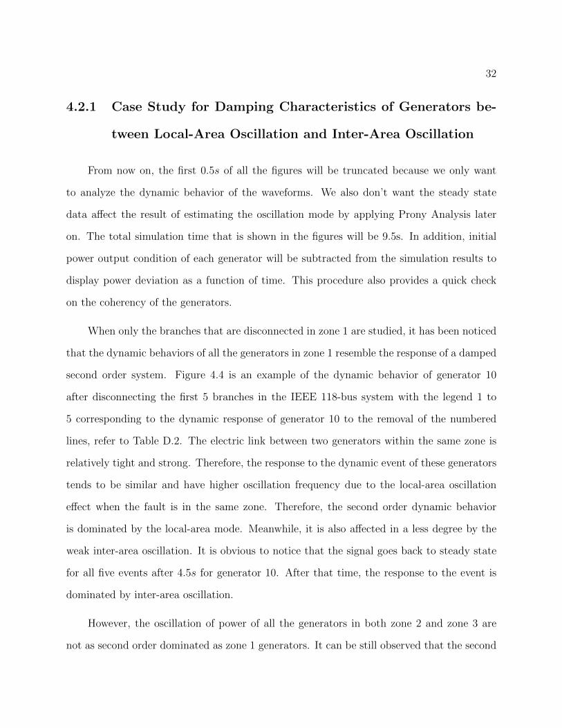
When only the branches that are disconnected in zone 1 are studied, it has been noticed

that the dynamic behaviors of all the generators in zone 1 resemble the response of a damped

second order system. Figure 4.4 is an example of the dynamic behavior of generator 10

after disconnecting the first 5 branches in the IEEE 118-bus system with the legend 1 to

5 corresponding to the dynamic response of generator 10 to the removal of the numbered

lines, refer to Table D.2. The electric link between two generators within the same zone is

relatively tight and strong. Therefore, the response to the dynamic event of these generators

tends to be similar and have higher oscillation frequency due to the local-area oscillation

effect when the fault is in the same zone. Therefore, the second order dynamic behavior

is dominated by the local-area mode. Meanwhile, it is also affected in a less degree by the

weak inter-area oscillation. It is obvious to notice that the signal goes back to steady state

for all five events after 4.5s for generator 10. After that time, the response to the event is

dominated by inter-area oscillation.

However, the oscillation of power of all the generators in both zone 2 and zone 3 are

not as second order dominated as zone 1 generators. It can be still observed that the second

33

0 1 2 3 4 5 6 7 8 9

time in s

-0.05

-0.04

-0.03

-0.02

-0.01

0

0.01

0.02

0.03

0.04

0.05

Pow

er in

p.u

.

Power of G10

12345

Figure 4.4: Dynamic Behavior of Power for G10 After Disconnecting First 5 Branches

order system behavior in the damped waveforms. It can be shown by randomly picking one

generator from zone 2 and one generator from zone 3 to display the dynamic behavior of

power with tripping first 5 lines in zone 1. The oscillation behavior of generator 61 in zone 2

is displayed in Figure 4.5. The oscillation behavior of generator 89 in zone 3 is illustrated in

Figure 4.6. It is observed from both Figure 4.5 and Figure 4.6 that the oscillation values of

power for all the events simulated in zone 2 and zone 3 are much smaller when compare to

the oscillation value of power in zone 1. Refer to Chapter 2, the larger network with a large

system inertia constant is harder to be perturbed than a smaller inertia constant in a smaller

network system. Therefore, the reason for the small oscillation values in the generators in

zone 2 and zone 3 is due to a swing against a larger network system than the generators in

zone 1. The oscillation lasts more than 9.5s to bring the system back to steady state again

for both zone 2 and zone 3. It takes more time to bring generator 61 and generator 89 back

34

0 1 2 3 4 5 6 7 8 9

time in s

-4

-3

-2

-1

0

1

2

3

4

Pow

er in

p.u

.

10-3 Power of G61

12345


0 1 2 3 4 5 6 7 8 9

time in s

-6

-4

-2

0

2

4

6

8

Pow

er in

p.u

.

10-3 Power of G89

12345


to steady state than generator 10 because the oscillation for both generator 61 and generator

89 are caused by both weak inter-area mode. Zone 1 and zone 2 are oscillating against each

35

other for generator 61. Zone 1 and Zone 3 are oscillating against each other for generator

89. It takes more time for generators to react on the events that are happening further away

due to longer distance and larger power system with a larger system inertia constant from

the perspective of the generators.

Similarly, when only the branches from branch 75 and 79 are disconnected in zone 2,

refer to Table D.1, are studied, the dynamic response for all the generators in zone 2 will

behave dominantly as a second order system. The simulation results for the generator 10 in

zone 1, generator 61 in zone 2, and generator 87 in zone 3 have been shown in Figure 4.7.

0 1 2 3 4 5 6 7 8 9

time in s

-5

0

5

Pow

er in

p.u

. 10-3 Power of G10

0 1 2 3 4 5 6 7 8 9

time in s

-0.2

0

0.2

Pow

er in

p.u

. Power of G61

0 1 2 3 4 5 6 7 8 9

time in s

-1

0

1

Pow

er in

p.u

. 10-3 Power of G87

Figure 4.7: Dynamic Behavior of Power After Disconnecting 5 Branches in Zone 2

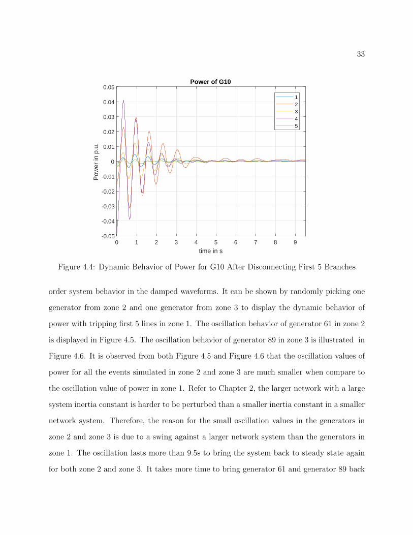
The same results are obtained for all the events happening in zone 3. The dynamic

simulation of disconnecting lines from branch 135 to 139 in zone 3 by looking into the

dynamic behavior of generators 25 in zone 1, generator 76 in zone 2, and generator 107 in

zone 3 are shown in Figure 4.8.

36

0 1 2 3 4 5 6 7 8 9

time in s

-0.01

0

0.01

Pow

er in

p.u

. Power of G25

0 1 2 3 4 5 6 7 8 9

time in s

-5

0

5

Pow

er in

p.u

. 10-3 Power of G76

0 1 2 3 4 5 6 7 8 9

time in s

-0.2

0

0.2

Pow

er in

p.u

. Power of G107

Figure 4.8: Dynamic Behavior of Power After Disconnecting 5 Branches in Zone 3

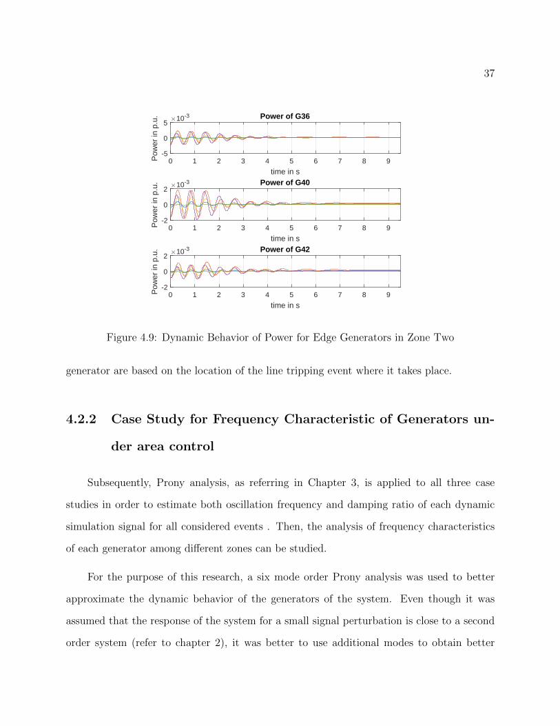
It was found that the generators near the boundary of two neighboring zones located

near tie-lines, will also present a response dominated by a second order damped system. For

example, generators 34, 36, 40, 42, 70, 72, 73, 74, and 76, which are located at the boundary

between zone 1 and zone 2, are tightly responding to zone 1 events. Some graphical behavior

of a few generators is illustrated in Figure 4.9 for zone 1 events. However, it can be noticed

that the damping amplitude is still smaller.

Therefore, when a generator that is connected to a large system, the dynamic behavior

of power for this generator is damped to be dominated by a second order system if a line

tripping occurs within the same zone area. Referring to Chapter 2, it is able to assume that

this generator is connected to an infinity bus, which is represented by a large network system

with a small signal disturbance based on the perspective of the generator. Since the initial

generator output power is mainly influenced by the machine inertia constant and machine

inertia constant is tightly related to oscillation frequency, the damping characteristics of each

37

0 1 2 3 4 5 6 7 8 9

time in s

-5

0

5

Pow

er in

p.u

. 10-3 Power of G36

0 1 2 3 4 5 6 7 8 9

time in s

-2

0

2

Pow

er in

p.u

. 10-3 Power of G40

0 1 2 3 4 5 6 7 8 9

time in s

-2

0

2

Pow

er in

p.u

. 10-3 Power of G42

Figure 4.9: Dynamic Behavior of Power for Edge Generators in Zone Two

generator are based on the location of the line tripping event where it takes place.

4.2.2 Case Study for Frequency Characteristic of Generators un-

der area control

Subsequently, Prony analysis, as referring in Chapter 3, is applied to all three case

studies in order to estimate both oscillation frequency and damping ratio of each dynamic

simulation signal for all considered events . Then, the analysis of frequency characteristics

of each generator among different zones can be studied.

For the purpose of this research, a six mode order Prony analysis was used to better

approximate the dynamic behavior of the generators of the system. Even though it was

assumed that the response of the system for a small signal perturbation is close to a second

order system (refer to chapter 2), it was better to use additional modes to obtain better

38

estimation in order to avoid noise and offset signal. In addition, high orders where tested

with results that did not prove to be a better estimation.

Thus, all the transient response of power, which is cause by suddenly disconnecting a

transmission line of power system for all 54 generators, is using 6 mode order to do Prony

analysis. In the Prony analysis, the transient response is sampled with 57 samples with

sampling rate of 6 Hz to create a discrete signal that corresponds to the simulation measure-

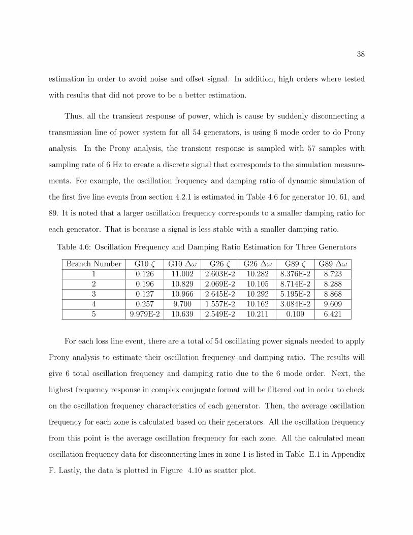
ments. For example, the oscillation frequency and damping ratio of dynamic simulation of

the first five line events from section 4.2.1 is estimated in Table 4.6 for generator 10, 61, and

89. It is noted that a larger oscillation frequency corresponds to a smaller damping ratio for

each generator. That is because a signal is less stable with a smaller damping ratio.

Table 4.6: Oscillation Frequency and Damping Ratio Estimation for Three Generators

Branch Number G10 ζ G10 ∆ω G26 ζ G26 ∆ω G89 ζ G89 ∆ω1 0.126 11.002 2.603E-2 10.282 8.376E-2 8.7232 0.196 10.829 2.069E-2 10.105 8.714E-2 8.2883 0.127 10.966 2.645E-2 10.292 5.195E-2 8.8684 0.257 9.700 1.557E-2 10.162 3.084E-2 9.6095 9.979E-2 10.639 2.549E-2 10.211 0.109 6.421

For each loss line event, there are a total of 54 oscillating power signals needed to apply

Prony analysis to estimate their oscillation frequency and damping ratio. The results will

give 6 total oscillation frequency and damping ratio due to the 6 mode order. Next, the

highest frequency response in complex conjugate format will be filtered out in order to check

on the oscillation frequency characteristics of each generator. Then, the average oscillation

frequency for each zone is calculated based on their generators. All the oscillation frequency

from this point is the average oscillation frequency for each zone. All the calculated mean

oscillation frequency data for disconnecting lines in zone 1 is listed in Table E.1 in Appendix

F. Lastly, the data is plotted in Figure 4.10 as scatter plot.

39

0 5 10 15 20 25 30 35 40

Branch Number

6

7

8

9

10

11

12

13

Are

a M

ean

Osc

illat

ion

Fre

quen

cy in

rad

/s

Area 1 Line Disconnecting

z1z2z3

Figure 4.10: Disconnecting Zone One Transmission Line

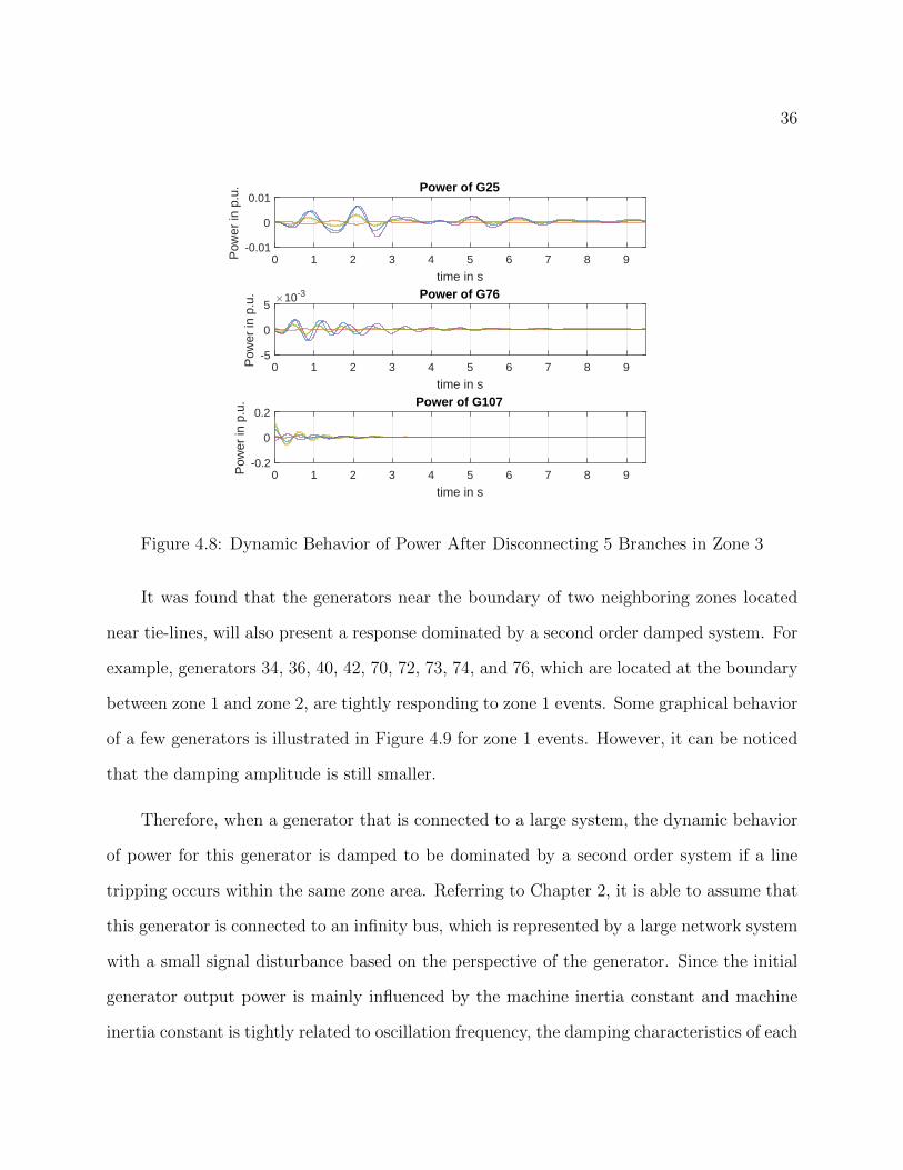
The discription of the Figure 4.10 is stated below:

• Each blue circle is the mean oscillation frequency value for generators in zone 1 for each

event. Almost all the blue circles are scattered at the top of the plot in Figure 4.10.

• Each red circle is the mean oscillation frequency value for generators in zone 2 for each

event. All the red circles are spreading around between blue circles and yellow circles.

• Each Yellow circle is the mean oscillation frequency value for generators in zone 3

for each event. All the yellow circles are distributed in the bottom of the plot in

Figure 4.10.

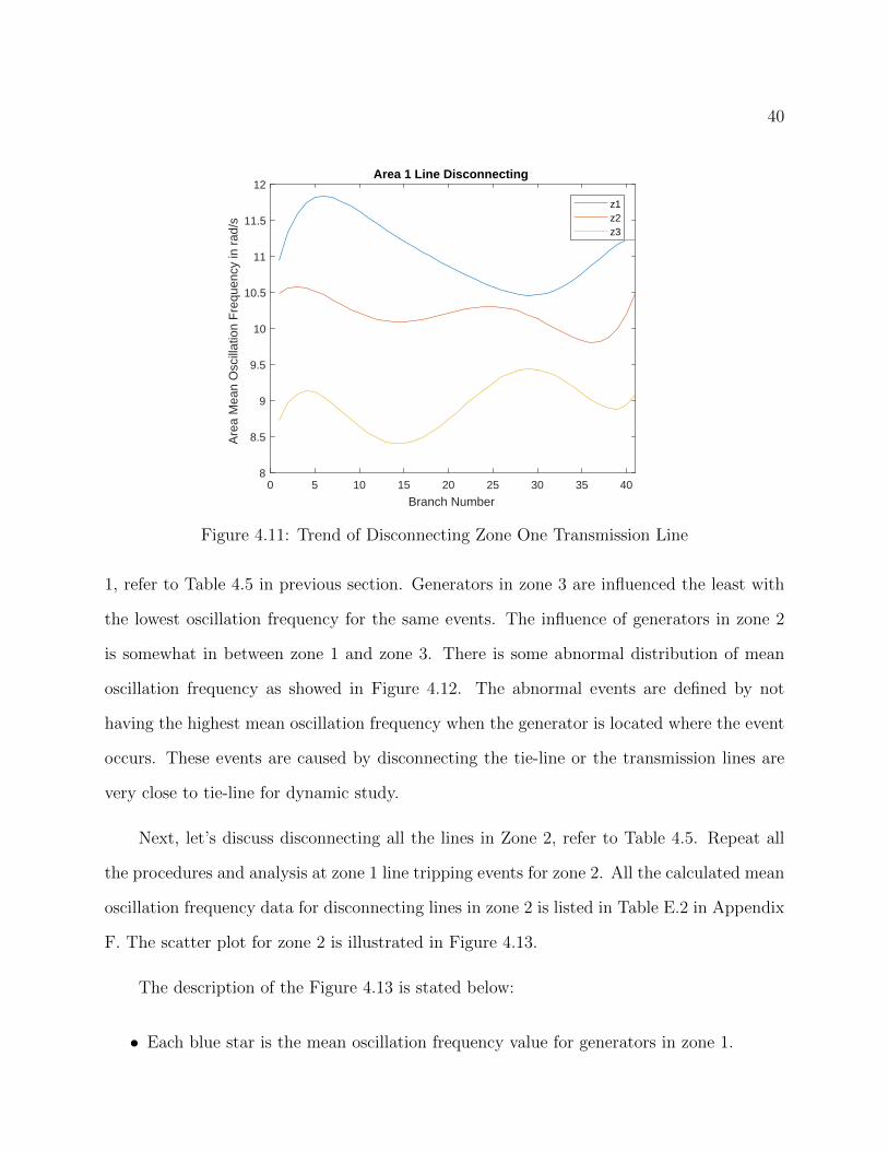
The trend of each zone can be derived by using polynomial curve fitting in matlab as

shown in Figure 4.11. The polynomial curve fitting finds the best fit in a least-square sense

for the data based on the degree of polynomial that best describe the curve.

Based on Figure 4.11, it indicates that the generators in zone 1 are influenced the most

with having the highest oscillation frequency by having disconnecting lines events in zone

40

0 5 10 15 20 25 30 35 40

Branch Number

8

8.5

9

9.5

10

10.5

11

11.5

12

Are

a M

ean

Osc

illat

ion

Fre

quen

cy in

rad

/s


z1z2z3

Figure 4.11: Trend of Disconnecting Zone One Transmission Line

1, refer to Table 4.5 in previous section. Generators in zone 3 are influenced the least with

the lowest oscillation frequency for the same events. The influence of generators in zone 2

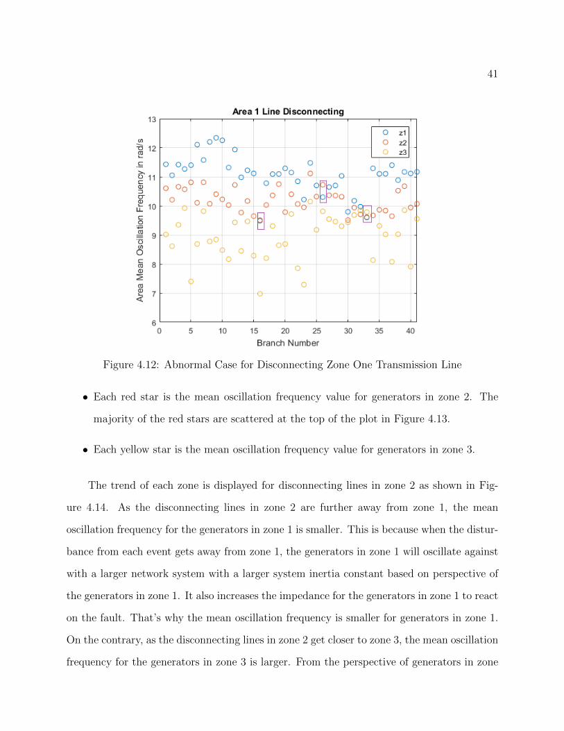
is somewhat in between zone 1 and zone 3. There is some abnormal distribution of mean

oscillation frequency as showed in Figure 4.12. The abnormal events are defined by not

having the highest mean oscillation frequency when the generator is located where the event

occurs. These events are caused by disconnecting the tie-line or the transmission lines are

very close to tie-line for dynamic study.

Next, let’s discuss disconnecting all the lines in Zone 2, refer to Table 4.5. Repeat all

the procedures and analysis at zone 1 line tripping events for zone 2. All the calculated mean

oscillation frequency data for disconnecting lines in zone 2 is listed in Table E.2 in Appendix

F. The scatter plot for zone 2 is illustrated in Figure 4.13.

The description of the Figure 4.13 is stated below:

• Each blue star is the mean oscillation frequency value for generators in zone 1.

41

Figure 4.12: Abnormal Case for Disconnecting Zone One Transmission Line

• Each red star is the mean oscillation frequency value for generators in zone 2. The

majority of the red stars are scattered at the top of the plot in Figure 4.13.

• Each yellow star is the mean oscillation frequency value for generators in zone 3.

The trend of each zone is displayed for disconnecting lines in zone 2 as shown in Fig-

ure 4.14. As the disconnecting lines in zone 2 are further away from zone 1, the mean

oscillation frequency for the generators in zone 1 is smaller. This is because when the distur-

bance from each event gets away from zone 1, the generators in zone 1 will oscillate against

with a larger network system with a larger system inertia constant based on perspective of

the generators in zone 1. It also increases the impedance for the generators in zone 1 to react

on the fault. That’s why the mean oscillation frequency is smaller for generators in zone 1.

On the contrary, as the disconnecting lines in zone 2 get closer to zone 3, the mean oscillation

frequency for the generators in zone 3 is larger. From the perspective of generators in zone

42

50 60 70 80 90 100

Branch Number

7.5

8

8.5

9

9.5

10

10.5

11

11.5

12

Are

a M

ean

Osc

illat

ion

Fre

quen

cy in

rad

/s


z1

z2

z3

Figure 4.13: Disconnecting Zone Two Transmission Line

3, they will oscillate against with a smaller network system with a smaller system inertia

constant. Moreover, it has shorter impedance for the generators in zone 3 to react on any

disturbance. When disconnecting lines around branch 100, refer to Table D.2 in Appendix

D, the oscillation frequency of generators in zone 3 is higher than generators in zone 2 due

to the border connection tie-lines and the lines that are near tie-lines are disconnected in

the system.

The result of disconnecting lines in zone 3 is very similar to the result of disconnecting

lines in zone 1 for the behaviors of generators in three different zones. The scatter plot

of this case is shown in Figure 4.15. The main difference is the behavior of generators in

zone 1 is opposite of the behavior of the generators in zone 3. The generators in zone 3

have the highest mean oscillation frequency when the lines are disconnected in zone 3. As

disconnecting lines for zone 3 move further away from zone 1, the mean oscillation frequency

43

50 60 70 80 90 100

Branch Number

8

8.5

9

9.5

10

10.5

11

11.5

Are

a M

ean

Osc

illat

ion

Fre

quen

cy in

rad

/s


z1z2z3

Figure 4.14: Trend of Disconnecting Zone Two Transmission Line

for generators in zone 1 is smaller. More abnormal events occur between zone 3 and zone 2

because they have more connections in the border or they have more tie-lines.

44

110 115 120 125 130 135 140

Branch Number

7.5

8

8.5

9

9.5

10

10.5

11

11.5

Are

a M

ean

Osc

illat

ion

Fre

quen

cy in

rad

/s


z1z2z3

Figure 4.15: Disconnecting Zone Three Transmission Line

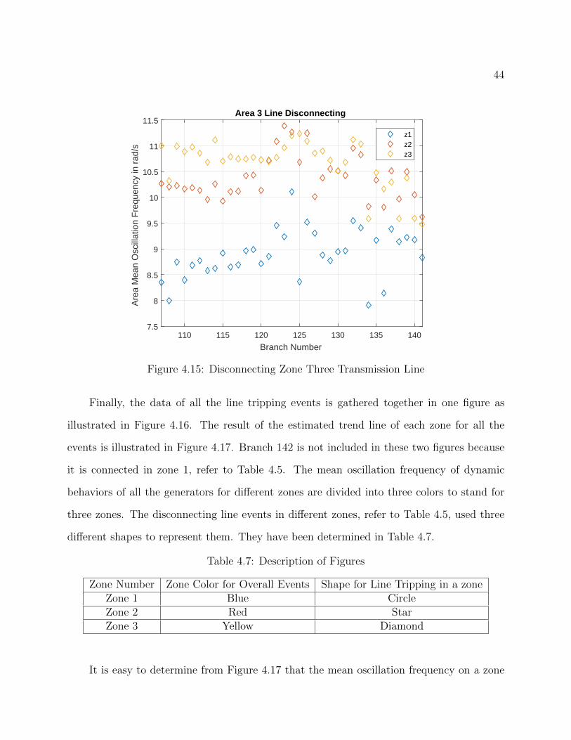
Finally, the data of all the line tripping events is gathered together in one figure as

illustrated in Figure 4.16. The result of the estimated trend line of each zone for all the

events is illustrated in Figure 4.17. Branch 142 is not included in these two figures because

it is connected in zone 1, refer to Table 4.5. The mean oscillation frequency of dynamic

behaviors of all the generators for different zones are divided into three colors to stand for

three zones. The disconnecting line events in different zones, refer to Table 4.5, used three

different shapes to represent them. They have been determined in Table 4.7.

Table 4.7: Description of Figures

Zone Number Zone Color for Overall Events Shape for Line Tripping in a zoneZone 1 Blue CircleZone 2 Red StarZone 3 Yellow Diamond

It is easy to determine from Figure 4.17 that the mean oscillation frequency on a zone

45

0 20 40 60 80 100 120 140

Branch Number

6

7

8

9

10

11

12

13

Are

a M

ean

Osc

illat

ion

Fre

quen

cy in

rad

/s

All Three Areas line Disconnecting

z1-1

z2-1

z3-1

z1-2

z2-2

z3-2

z1-3

z2-3

z3-3

Figure 4.16: Disconnecting All 142 Branches

has the highest reading when the line is disconnected in the same zone area. In addition,

when the transmission line is disconnected from the system and is moving further away from

a zone, the mean oscillation frequency of that zone decreases. When a disconnected line from

the system is moving closer to a zone, the mean oscillation frequency of that zone increases.

The mean oscillation frequency of zone 1 is flat in the very beginning because the line

is tripped in its own zone. Then it is decreasing all the way as the line is tripped is moving

away from zone 1. The mean oscillation frequency of zone 2 generators is like the shape of

an arch because the tripped line is getting closer to zone 2 from zone 1 to zone 2 and then

away from zone 2 to zone 3. The mean oscillation frequency of zone 3 is increasing as the

line is tripped from zone 1 to zone 3. It gets flat again when the line is tripped in the same

zone.

46

0 20 40 60 80 100 120 140

Branch Number

8

8.5

9

9.5

10

10.5

11

11.5

Are

a M

ean

Osc

illat

ion

Fre

quen

cy in

rad

/s

All Transmision Lines Disconnecting

z1z2z3

Figure 4.17: Disconnecting All 142 Branches

The oscillation frequency range for each zone in Table 4.8 is in radians and Table 4.9

is in Hz under three case studies, which is disconnecting three groups of transmission lines

refer to Table 4.5.

Table 4.8: Mean Oscillation Frequency Range in Radians for Three Zones under ThreeStudies

Z1 line ωmax Z1 line ωmin Z2 line ωmax Z2 line ωmin Z3 line ωmax Z3 line ωminZone 1 12.3434 9.4898 10.9942 7.8614 10.1089 7.9088Zone 2 11.1143 9.5094 11.6425 9.8831 11.3891 9.6189Zone 3 10.1479 6.9816 11.4495 8.2215 11.2341 9.4802

Table 4.9: Mean Oscillation Frequency Range in HZ for Three Zones under Three Studies

Z1 line fmax Z1 line fmin Z2 line fmax Z2 line fmin Z3 line fmax Z3 line fminZone 1 1.964 1.510 1.750 1.251 1.609 1.259Zone 2 1.769 1.513 1.859 1.573 1.812 1.531Zone 3 1.615 1.111 1.822 1.308 1.788 1.509

47

Once again, when the line that is tripped moves away from a zone, both maximum and

minimum values of mean oscillation frequency become smaller and the oscillation frequency

range is shifting. It is the same for all three studies. The zone where the line is tripped has

the highest oscillation frequency. The zone where the line is tripped is the furthest away has

the lowest oscillation frequency. As a result, the larger system inertia constant will be seen

by a generator as the event that it occurs is further away from the generator. The larger

system inertia constant minimizes the frequency oscillation. Therefore, the larger system

inertia constant will make the power system more stable with lower oscillation frequency.

Chapter 5

Conclusion and Future Work

5.1 Conclusion

With the rapid development of integrating the renewable energy in the power system,

the relationship between frequency characteristics of generators and system inertia constant

H will take more responsibility on frequency regulation for the power system. The primary

purpose of this thesis was to analyze the frequency and damping characteristics of generators

in the power systems through dynamic simulation of generator output power when a line is

tripped.

This report used simulation studies and derived theoretical analysis to study that a

generator connected to a large network system can be represented as the single-machine

infinite bus from the perspective of the generator. From the analysis, it is noted that the

location of the line tripping is very critical. The simulation results concluded that the

represented SMIB system is recognized as a second order damped system when the line

tripping occurred in the same area as the generator, or the generators of neighboring zones

located near a tie-line. It is recognized that the larger system inertia constant will be seen

by a generator as the event that it occurs is further away from that generator. It is further

48

49

recognized that perturbation of dynamic damping for the initial generator output power for

these generators are smaller because the system becomes more stable with larger system

inertia constant from the perspective of the generator.

The dynamic simulation studies demonstrate that the oscillation frequency of generator

output power has its own range for each zones when a line is tripped in different zones.

The magnitude of oscillation frequency of each zone for each line loss event is based on the

proximity of the loss line event takes place from the zone. The zone with the fault occurs has

the highest oscillation frequency. The zone that is the furthest away from the fault occurs

has the lowest oscillation frequency.

Clearly, both frequency and damping characteristics of generators are highly relevant

to 2 factors as described below:

• the location of the disturbance

• the amount of damping associated to the oscillation

According to the analysis described previously, frequency and damping characteristics

of generators are highly depended on the system inertia constant. Thus, the higher inertia

constant is a critical factor to ensure the system is to be more stable and avoid to be

perturbed.

5.2 Future Work

Future research work may be performed on the stability study of the power system by

checking on the system damping ratio of the system. By defining the smallest system damp-

ing ratio that can be reached in order to keep the oscillation frequency of the system within

50

the stability range of the system. Then, the stability of a power system can be controlled by

controlling the system damping ratio. Further, the sensitivity study of frequency character-

istics of generators can be approached by adding different renewable source into the power

system. Further research is needed in order to estimate the system inertia constant from the

perspective of a generator when is connected to a large network system.

Bibliography

[1] M. Klein, G.J. Roger, P. Kundur. “A Fundamental Study of Inter-area Oscillation inPower Systems.” IEEE Transictions on Power Systems., vol. 6, no. 3, Aug. 1991.

[2] P. M. Anderson, M. Mirheydar. “A Low-order System Frequency Response Model.”IEEE Transictions on Power Systems., vol. 5, no. 3,pp. 720-729, Aug. 1990.

[3] B. K. Kumar. “Power System Stability and Control.” 2012.

[4] P. M. Anderson, M. Mirheydar. “An Adaptive Method for Setting Underfrequency LoadShedding Relays.” IEEE Transictions on Power Systems., vol. 7, no. 3,pp. 647-655, May1992.

[5] H. Saadat. “Power System Analysis.” McGraw Hill 2nd Edition, 2002.

[6] H. Huang, F. Li. “Sensitivity Analysis of Load-Damping Characteristic in Power SystemFrequency Regulation.” IEEE Transactions on Power Systems. vol. 28, no. 2, pp. 1324-1335, May 2013.

[7] V. Terzija. “Adaptive Underfrequency Load Shedding Based on the Magnitude ofthe Disturbance Estimation.” 2007 IEEE Power Engineering Society General Meeting.Tampa, FL, 2007, pp. 1-1.

[8] P. W. Sauer, M. A. Pai. “Power System Dynamics and Stability.” Prentice Hall, 1998

[9] W. D. Stevenson. “Element of Power System Analysis.” McGraw-Hill, 1982

[10] A. Ulbig, T. S. Borsche, G. Andersson. “Impact of Low Rotational Inertia on PowerSystem Stability and Operation.” IFAC World Congress 2014., Dec. 2014.

[11] M. A. Pai, A. M. StankovicJ. H. Chow. “Penquoteower Electronics and Power Systems.”Springer, Vol. 95, 2013.

[12] “PSS/E 34 Model Library.” Siemens Industry. March, 2015.

[13] “Modeling Notification.” North American Electric Reliability Corporation. March, 2015.

51

52

[14] J. F. Hauer, C. J. Demeure, and L. L. Scharf. “Initial Results in Prony Analysis ofPower System Response Signals.” IEEE Trans. on Power Syst., vol. 5, no. 1, pp.80-89,Feb. 1990.

[15] C. Ray, Z. Huang. “Power Grid Dynamic: Enhancing Power System Operation ThroughProny Analysis.” Journal of Undergraduate Research., Jan. 2007.

[16] “Vandermonde Matrix.” https://en.wikipedia.org/wiki/Vandermonde˙matrix.

[17] “Toeplitz˙matrix.”https://en.wikipedia.org/wiki/Toeplitz˙matrix.

[18] “Illinois Center for A Smarter Electric Grid (ICSEG).” University of Illinois. 2013. Fromhttp://icseg.iti.illinois.edu/ieee-118-bus-system/

[19] R. Rocchetta, E. Patelli.“Power Grid Robustness Failures: Topological and Flow BasedMetric Comparison.” ECCOMAS Congress 2016. 2016

[20] G. W. Stagg, A. H. El-Abiad. “Computer Method in Power System Analysis.” McGraw-Hill, Vol. 95, 2013.

Appendices

53

Appendix A

Model of Exciter

Figure A.1: IEEET1˙Exciter

Parameters Ranges:0 ≤ TR < 0.5 − 1 ≤ KE ≤ 1< KA < 500 0.04 < TE < 10 ≤ TA < 1 0 < KF < 0.30.5 < VRMAX < 10 0.04 < TE < 1.5−10 < VRMIN < 0 5 < TF/KF/ge15

54

55

Table A.1: IEEE Type 1 Excitation System - IEEET1

Parameters Value Description

TR 0.06 Filter time constant in secondKA 20 Regulator gain in p.u.TA 0.01 Regulator time constant in second

VRMAX 5.0 Maximum voltage regulator outputs in p.u.VRMIN -6.0 Minimum voltage regulator outputs in p.u.KE 1.0 Exciter constant related to self-excited field

TE 0.67Exciter time constant, integration rate associated with

exciter control in secondKF 0.1 Feedback gainTF 1.0 Feedback time constant

Switch 0.0Exciter alternator output voltages back of commutating

reactance at which saturation is defined

E1 3.0Exciter saturation function value at the corresponding

exciter voltage, E1, back of commutating reactance

SE(E1) 0.09Exciter alternator output voltages back of commutating

reactance at which saturation is definedE2 4.0 stator leakage reactance

SE(E2) 0.368Exciter saturation function value at the corresponding exciter

voltage, E2, back of commutating reactance

Appendix B

Model of Governor

Figure B.1: Steam˙Turbine˙Governor

Table B.1: Steam turbine-governor model - TGOV1

Parameters Values Description

R 0.04 Permanent droop in p.u.T1 0.4 Steam bowl time constant in second

VMAX1 Maximum valve position in p.u.

VMIN1 -1.0 Minimum valve position in p.u.

T22 1.5 time constant in second

T33 5.0 time constant in second

Dt1 0.0 Turbine damping coefficient in p.u.

1VMAX, VMIN, Dt and R are in per unit on generator MVA base.2T2/T3 = high-pressure fraction.3T3 = reheater time constant.

56

57

Parameters Range:0 < R < 0.1 0 < T2

0.04 < T1 < 0.5 004 < T3 < 10.00.5 ≤ VMAX ≤ 1.2 T2 < T3/2.0VMIN < VMAX 0 ≤ DT < 0.50 ≤ VMIN < 1.0

Appendix C

Bus Incidence Matrix

Figure C.1: Incidence Matrix Part1

58

59

Figure C.2: Incidence Matrix Part2

It is difficult to display the values of the matrix due to the large matrix for the bus incidencematrix with dimension 186× 118. Also, the matrix has to divide into two figures in order todisplay the full matrix. The color code has been used in this matrix. The cyan representsvalues 0, the yellow represents value 1, and the blue stands for value -1 in both figure C1and figure C2.

C.1 Matlab Code for Bus Incidence Matrix

1 c l c ;2 c l e a r ;3

4 %% Read e x c e l f o r a l l connect ing braches between two buses .

60

5 data = x l s r e ad ( ’ Tr ip Line Data Source IEEE118 Or ig ina l 10 18 . x l sx ’) ;

6 A = ze ro s (186 ,118) ;7 co l 1 = data ( : , 1 ) ;8 co l 2 = data ( : , 2 ) ;9 count = 1 ;

10 count2= 0 ;11 num = length ( co l 1 ) ;12 %%% Assign a i j va lue s13 f o r i = 1 :num14 A( i , c o l 1 ( i , 1 ) ) = 1 ;15 A( i , c o l 2 ( i , 1 ) ) = 1 ;16 end17 %% Output i s l a n d bus18 f o r i = 1:11819 i f sum( abs (A( : , i ) ) ) == 120 output ( count ) = i ;21 count = count + 1 ;22 end23 end24 Cname = 1 : 1 : 1 1 8 ;25 sz = s i z e (Cname) ;26 Scname = s t r i n g s ( sz ) ;27 f o r i = 1:11828 Scname ( i ) = s t r i n g ( i ) ;29 end30 %%% di sp l ay a matrix in a matlab GUI tab l e .31 f i g u r e (1 ) ;32 t = u i t a b l e ( ’ColumnName ’ , Scname ) ;33 s e t ( t , ’ Data ’ , A)34 %%% Use Image to r e p r e s e n t the matrix35 f i g u r e (2 )36 h = imagesc (A)37 imp ix e l r e g i on (h)38 f i g u r e (3 )39 t ab l e (A)

Appendix D

186 Branches from IEEE 118-Bus

Table D.1: 186 Branches from IEEE 118-Bus

Branch From˙Bus To˙Bus Branch From˙Bus To˙Bus1 1 2 25 16 172 1 3 26 17 183 2 12 27 17 314 3 5 28 17 1135 3 12 29 18 196 4 5 30 19 207 4 11 31 19 348 5 6 32 20 219 5 11 33 21 2210 6 7 34 22 2311 7 12 35 23 2412 8 9 36 23 2513 8 30 37 23 3214 9 10 38 24 7015 11 12 39 24 7216 11 13 40 25 2717 12 14 41 26 3018 12 16 42 27 2819 12 117 43 27 3220 13 15 44 27 11521 14 15 45 28 2922 15 17 46 29 3123 15 19 47 30 3824 15 33 48 31 32

61

62


Branch From˙Bus To˙Bus Branch From˙Bus To˙Bus49 32 113 87 54 5550 32 114 88 54 5651 33 37 89 54 5952 34 36 90 55 5653 34 37 91 55 5954 34 43 92 56 5755 35 36 93 56 5856 35 37 94 56 5957 37 39 95 56 5958 37 40 96 59 6059 38 65 97 59 6160 39 40 98 60 6161 40 41 99 60 6262 40 42 100 61 6263 41 42 101 62 6664 42 49 102 62 6765 42 49 103 63 6466 43 44 104 64 6567 44 45 105 65 6868 45 46 106 66 6769 45 49 107 68 8170 46 47 108 68 11671 46 48 109 69 7072 47 49 110 69 7573 47 69 111 69 7774 48 49 112 70 7175 49 50 113 70 7476 49 51 114 70 7577 49 54 115 71 7278 49 54 116 71 7379 49 66 117 74 7580 49 66 118 75 7781 49 69 119 75 11882 50 57 120 76 7783 51 52 121 76 11884 51 58 122 77 7885 52 53 123 77 8086 53 54 124 77 80

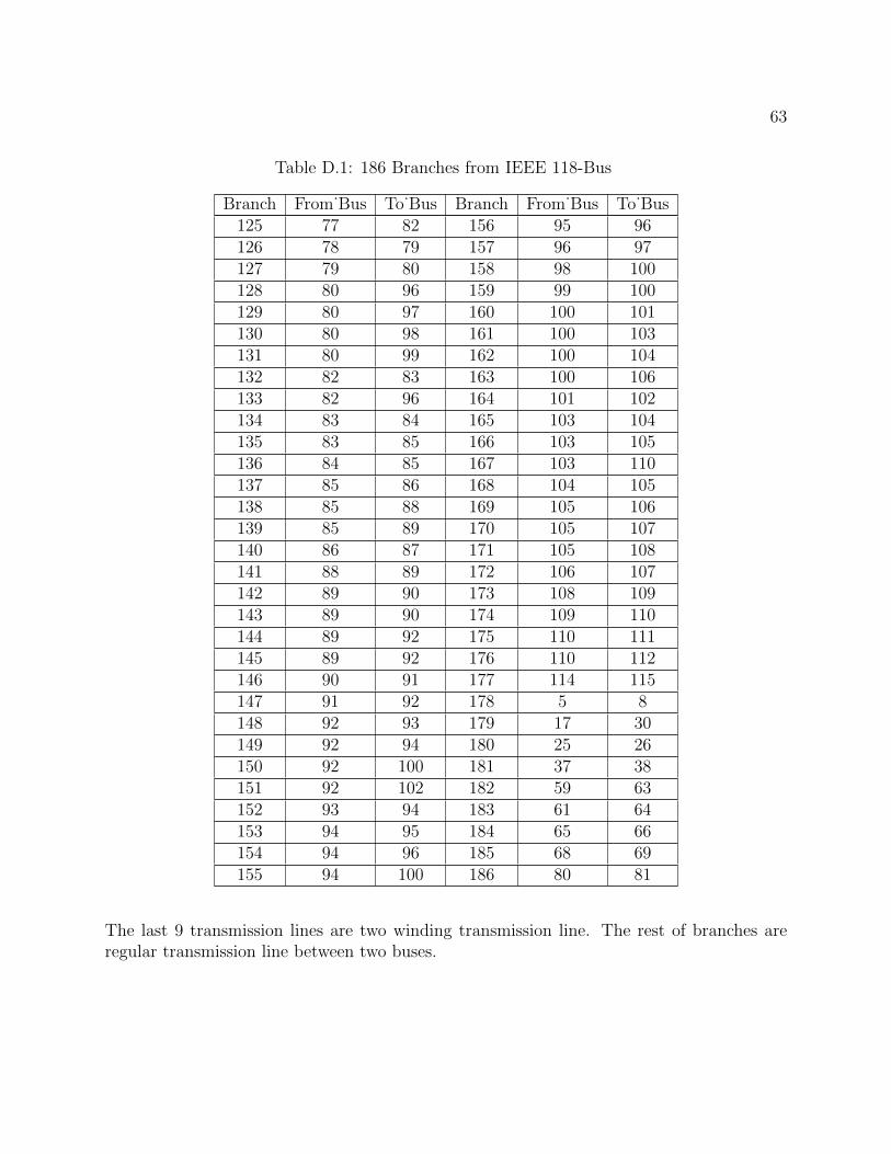
63


Branch From˙Bus To˙Bus Branch From˙Bus To˙Bus125 77 82 156 95 96126 78 79 157 96 97127 79 80 158 98 100128 80 96 159 99 100129 80 97 160 100 101130 80 98 161 100 103131 80 99 162 100 104132 82 83 163 100 106133 82 96 164 101 102134 83 84 165 103 104135 83 85 166 103 105136 84 85 167 103 110137 85 86 168 104 105138 85 88 169 105 106139 85 89 170 105 107140 86 87 171 105 108141 88 89 172 106 107142 89 90 173 108 109143 89 90 174 109 110144 89 92 175 110 111145 89 92 176 110 112146 90 91 177 114 115147 91 92 178 5 8148 92 93 179 17 30149 92 94 180 25 26150 92 100 181 37 38151 92 102 182 59 63152 93 94 183 61 64153 94 95 184 65 66154 94 96 185 68 69155 94 100 186 80 81

The last 9 transmission lines are two winding transmission line. The rest of branches areregular transmission line between two buses.

64


Branch From˙Bus To˙Bus Branch From˙Bus To˙Bus1 1 2 39 31 322 1 3 40 32 1133 2 12 41 32 1144 3 5 42 33 375 3 12 43 34 366 4 11 44 34 437 5 6 45 35 368 5 11 46 35 379 6 7 47 37 3910 7 12 48 37 4011 8 30 49 39 4012 11 12 50 40 4113 11 13 51 40 4214 12 14 52 41 4215 12 16 53 43 4416 13 15 54 44 4517 14 15 55 45 4618 15 19 56 45 4919 15 33 57 46 4720 16 17 58 46 4821 17 18 59 47 4922 17 31 60 47 6923 17 113 61 48 4924 18 19 62 49 5025 19 20 63 49 5126 19 34 64 49 5427 20 21 65 49 6928 21 22 66 50 5729 22 23 67 51 5230 23 24 68 51 5831 23 32 69 52 5332 24 70 70 53 5433 24 72 71 54 5534 27 28 72 54 5635 27 32 73 54 5936 27 115 74 55 5637 28 29 75 55 5938 29 31 76 56 57

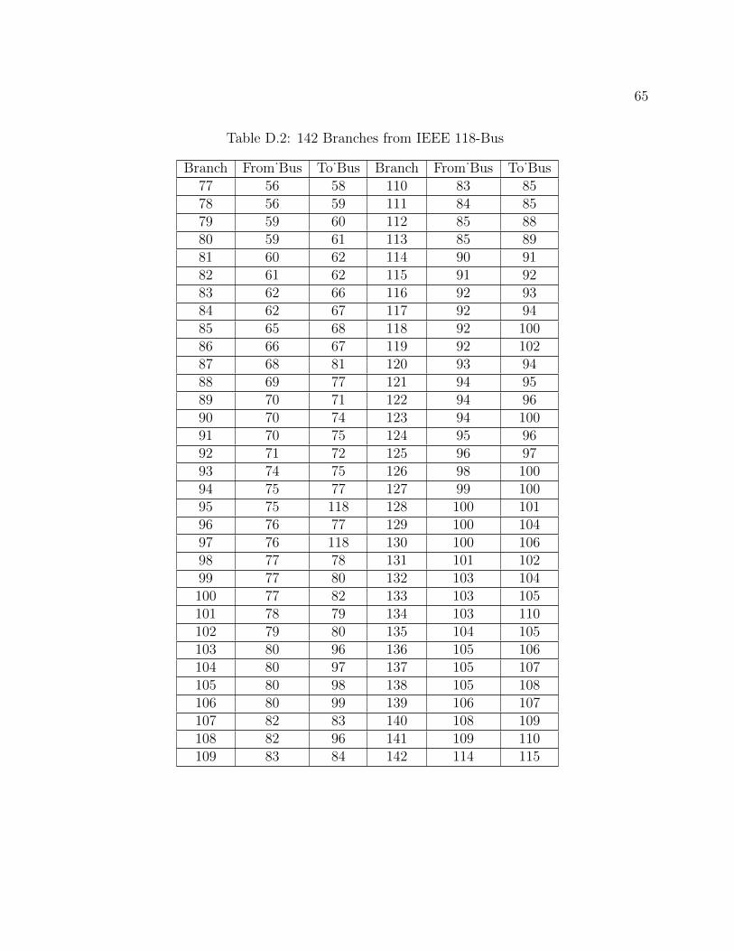
65


Branch From˙Bus To˙Bus Branch From˙Bus To˙Bus77 56 58 110 83 8578 56 59 111 84 8579 59 60 112 85 8880 59 61 113 85 8981 60 62 114 90 9182 61 62 115 91 9283 62 66 116 92 9384 62 67 117 92 9485 65 68 118 92 10086 66 67 119 92 10287 68 81 120 93 9488 69 77 121 94 9589 70 71 122 94 9690 70 74 123 94 10091 70 75 124 95 9692 71 72 125 96 9793 74 75 126 98 10094 75 77 127 99 10095 75 118 128 100 10196 76 77 129 100 10497 76 118 130 100 10698 77 78 131 101 10299 77 80 132 103 104100 77 82 133 103 105101 78 79 134 103 110102 79 80 135 104 105103 80 96 136 105 106104 80 97 137 105 107105 80 98 138 105 108106 80 99 139 106 107107 82 83 140 108 109108 82 96 141 109 110109 83 84 142 114 115

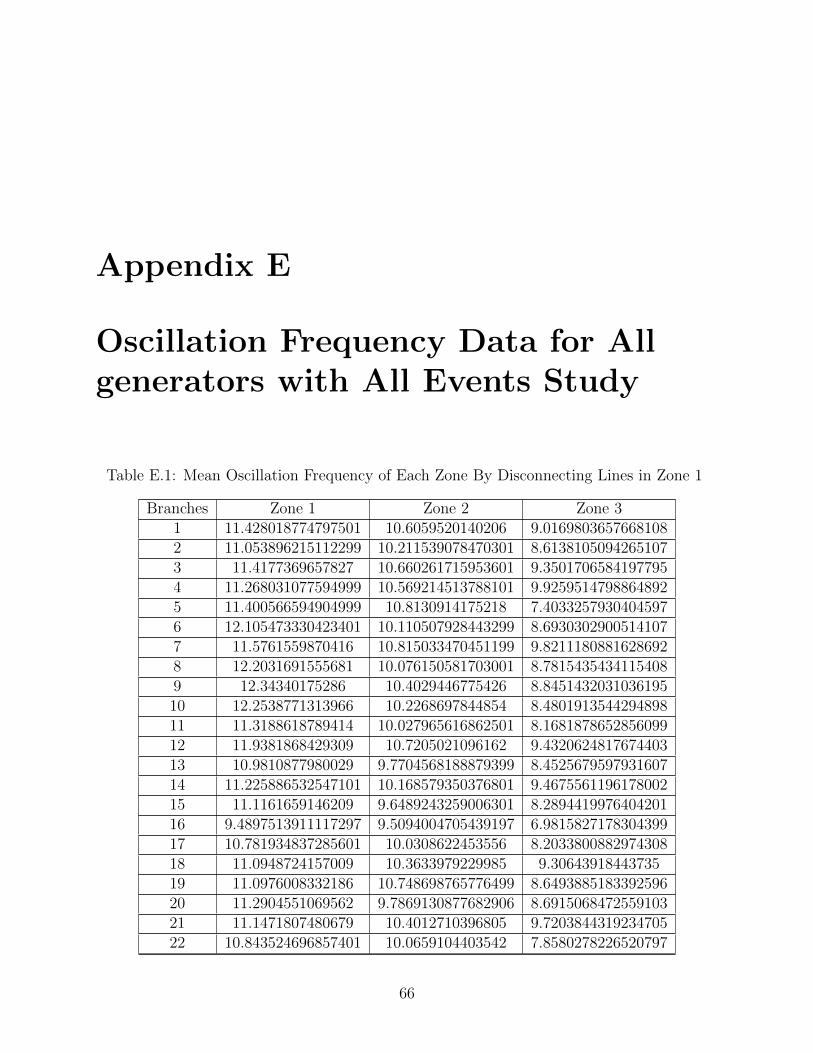
Appendix E

Oscillation Frequency Data for Allgenerators with All Events Study

Table E.1: Mean Oscillation Frequency of Each Zone By Disconnecting Lines in Zone 1

Branches Zone 1 Zone 2 Zone 31 11.428018774797501 10.6059520140206 9.01698036576681082 11.053896215112299 10.211539078470301 8.61381050942651073 11.4177369657827 10.660261715953601 9.35017065841977954 11.268031077594999 10.569214513788101 9.92595147988648925 11.400566594904999 10.8130914175218 7.40332579304045976 12.105473330423401 10.110507928443299 8.69303029005141077 11.5761559870416 10.815033470451199 9.82111808816286928 12.2031691555681 10.076150581703001 8.78154354341154089 12.34340175286 10.4029446775426 8.845143203103619510 12.2538771313966 10.2268697844854 8.480191354429489811 11.3188618789414 10.027965616862501 8.168187865285609912 11.9381868429309 10.7205021096162 9.432062481767440313 10.9810877980029 9.7704568188879399 8.452567959793160714 11.225886532547101 10.168579350376801 9.467556119617800215 11.1161659146209 9.6489243259006301 8.289441997640420116 9.4897513911117297 9.5094004705439197 6.981582717830439917 10.781934837285601 10.0308622453556 8.203380088297430818 11.0948724157009 10.3633979229985 9.3064391844373519 11.0976008332186 10.748698765776499 8.649388518339259620 11.2904551069562 9.7869130877682906 8.691506847255910321 11.1471807480679 10.4012710396805 9.720384431923470522 10.843524696857401 10.0659104403542 7.8580278226520797

66

67


Branches Zone 1 Zone 2 Zone 323 10.2199355618026 9.9537665150290504 7.294390714604410224 11.480290542771799 11.1143139565017 10.14794239552125 10.702325342296101 10.318631636242699 9.177190520465940126 10.3003262855963 10.726870056652899 9.816967327247940727 10.6512213258302 10.3689241556922 9.546942748435130428 10.702124648383901 10.3575112472125 9.458464848000000229 11.031068376543701 10.3139899886748 9.300489460941690830 9.8001005658942706 9.5151442328105205 9.434143087820629631 10.174652839972399 9.94431802171143 9.685853451229350632 9.9736588942696898 9.7101795245330802 9.847202103319769933 9.5989521359475898 9.6127608843380603 9.7904966848645534 11.289988562749601 9.6756427123495303 8.136083870645439535 11.1030553495516 9.8647545321276802 9.313840473444459536 11.105088481332 9.83745092410539 9.020514661377200537 11.3995134619565 9.6497836226000402 8.081543862064670238 10.8865284113215 10.5272112400952 9.025267316976780339 11.168300688210699 10.6784970268133 9.852034353382709540 11.115522813330999 9.9479015891673299 7.911093755652739641 11.171761698772199 10.0741161046545 9.5550529891451905142 11.3089677556884 11.2307054508848 11.434730201558599


Branches Zone 1 Zone 2 Zone 342 10.7236587895495 10.7456818091072 8.423967920187180943 10.9941707867024 11.3989634122625 10.29597934393049944 10.176999088588 10.9633796855046 8.221535453697260545 10.2657483777216 11.4820482645898 10.76703047032900146 10.974666767797601 11.3379398489186 10.40903338960447 10.913652532251399 11.023164660718701 9.845642494362589848 10.9536627081592 11.0492557047099 9.852471690574029549 10.9677273694299 11.0743039161121 9.931171428647699550 10.4309936778187 11.0884456732316 9.983826810647839251 10.615555029921101 11.3895547689553 9.122237096642939152 10.608949718988899 11.3965339685133 9.025549969687759253 10.5906937273084 10.897273212323 9.642828651299810354 10.3300353402475 10.8813624031029 9.411474505901020755 10.7176026482897 11.0524362321061 9.8949310543879996

68


Branches Zone 1 Zone 2 Zone 356 10.4039591032949 11.3581476017987 9.301238512249799657 9.9342054672367492 11.2765606934134 10.445346250487558 10.0577881678221 11.442608799756099 10.652493861002159 9.54860766106294 11.0172452491316 9.677693648871210660 9.6620002138238092 10.7710327877887 10.132215456870461 10.2224948934675 11.506156532455501 10.56180540179419962 10.2757455056061 10.9505584010878 10.042259268472663 10.2613545873534 10.9107051536149 10.01947498671309964 10.2762124722996 10.9700891248267 10.05258722803879965 9.5479767135926199 10.8186014140782 10.06077180254649966 10.270856717152199 10.9622882187985 10.04694214207039967 10.3967807772194 11.131245137460301 10.090228758049868 10.315064022471301 10.987376333350401 10.09674429639619969 10.5082863733795 11.408563898372901 10.08635570561889970 10.1212528790621 10.919291811754301 9.952642574191610771 10.887009434400699 11.106215622454901 11.17779278376539972 10.4202302985295 11.0514801408036 10.072649594254173 10.4208570449838 10.860674480198901 10.74187390436629974 10.304654156857699 11.232416279142701 10.143132620913175 10.417617101190499 10.9988690869635 10.81215592086980176 10.267416431143999 10.9659106753438 10.077757430873377 10.421737811510701 11.027915533691401 10.063481863473278 10.433787176866399 10.947907036587701 10.797218857536879 9.8478395036930895 10.887571930421499 10.37168996078209980 9.8331151149409095 10.908130081759801 10.369053936002781 10.736536467677301 11.6824873223132 10.29978783436149982 10.613890417156499 11.635396125509599 10.389928023939283 10.263579461225699 11.1509023935981 10.01158118568984 10.335208304441601 11.4120987297573 10.08766993094739985 9.7244016524374608 11.413628979169401 9.906268754464440186 10.2604638306055 11.086971060977501 10.009314637132787 9.0551497987275091 10.741925183964399 10.86176450721709988 9.8731452767504599 11.0650544822927 11.14598885525279989 8.76790383732639 9.8830913270408001 9.937896804451909890 8.7091550167021996 10.272695876053501 10.456707738784191 9.6469793456673791 10.568330418473799 10.543188045100892 8.7210454611775603 9.9768966709688094 10.142084461773993 8.7047060923743302 10.295786893547699 10.0490838765521

69


Branches Zone 1 Zone 2 Zone 394 8.6731806004369396 10.719604606163299 11.01428526875439995 9.1439960072322002 10.5418147549819 10.399902203229896 8.7131973767154793 10.420077405233 10.567727336177797 9.10083367645659 10.536155451192 10.481660183785398 8.7857999592554901 11.1022212563373 11.02632781992100199 8.7783176675274603 11.224338990744901 11.265767872263099100 7.8614094271646398 10.1576409714229 9.1900931463403293101 8.7422519749800909 11.081224386398199 11.098344724612099102 8.7546913096807799 11.204387658421201 11.0817839996675103 8.4607259579356899 10.7420659140118 11.416524640050399104 8.4292542394209509 10.7405482428317 11.449485123334499105 9.2104853185210391 11.019174955019301 10.9170877813625106 9.3503881834633393 11.130691130448801 10.8659862794118


Branches Zone 1 Zone 2 Zone 3107 8.3512955743615507 10.266557779882501 11.000716728710101108 7.9975877577847099 10.204530601801199 10.3234001428402109 8.74716789606269 10.224574798738599 10.991706685338199110 8.3966958678039099 10.167116967172101 10.888206091600701111 8.6830882608552091 10.186679834734599 10.978546858517401112 8.7767684502563608 10.140517955895801 10.858777184006099113 8.5784140591673097 9.9607549202714107 10.680895101336899114 8.6225340043279495 10.2596384321947 11.1170510335016115 8.9189210395581995 9.9266210644145492 10.707550470578401116 8.6526651463738098 10.1111644578121 10.7839993827212117 8.6911618907120491 10.1206039547759 10.745377861947601118 8.9648994083340501 10.4237520097944 10.7440178130595119 8.9847337447978095 10.4322738574003 10.7798189582099120 8.7106946510818997 10.1371018307723 10.7280375409697121 8.8560435610767403 10.7212068937885 10.7008326932496122 9.4550039956720706 11.085785504457601 10.772036043267599123 9.24090579483269 11.3891389886618 10.963809578625201124 10.1089108296128 11.270597263144801 11.197151335626099125 8.3620977162884405 10.685818549891 11.234072118554399126 9.5160863695642597 11.246257406134999 11.090119662693899127 9.3049219013946196 10.01822658122 10.858854826843199

70


Branches Zone 1 Zone 2 Zone 3128 8.8852125305000893 10.3789028867024 10.8995047888912129 8.7753144964650804 10.551056959632801 10.7188744378879130 8.9426224365160394 10.510970740918101 10.516774703319101131 8.9645554136265009 10.4280417914837 10.6861613667276132 9.5471881442096596 10.9565930110276 11.119150132706133 9.4095587390832698 10.8249466567715 11.035875929244501134 7.90884197022483 9.8220340737013903 9.5875521263963002135 9.1725487378636803 10.334473302241999 10.4803485594076136 8.1402461843048393 9.8100171843159796 10.166565626699599137 9.3861394659197295 10.5111541412082 10.294093329224699138 9.1448352901039396 9.9695308012687995 9.58748243137582139 9.2237881331799105 10.495936506048199 10.374647511159701140 9.1762236620569499 10.0490197322172 9.5946648102309897141 8.8330831747654699 9.6189338424769097 9.4801754931089999

frequency and damping characteristics of … as a generator connects to a large network system with...

Documents