freeway rear-end collision risk for italian freeways. an...
TRANSCRIPT

XXII SIDT
National Scientific Seminar
Politecnico di Bari
14 – 15 SETTEMBRE 2017
Freeway rear-end collision risk for Italian freeways.
An extreme value theory approach
Gregorio Gecchele
Federico Orsini
University of Padova
University of Padova

2
• Main concepts
• Focus of the paperFreeway rear-end
collision risk
• Proposed Approach
• Experimental Analysis
• Analysis of Results
The study
Theory and Practice
• Concluding Remarks
• Future DevelopmentsConclusions
Outline

3
• Main concepts
• Focus of the paperFreeway rear-end
collision risk
• Proposed Approach
• Experimental Analysis
• Analysis of Results
The study
Theory and Practice
• Concluding Remarks
• Future DevelopmentsConclusions

4
Freeway rear-end collision risk.Main concepts & focus of the paper
Motivations
• Safety analysis is a relevant activity in transportation planning
• Road safety analysis traditionally is based on crash data.
• However, the use of crash data has several shortcomings:– under-reporting and frequent problems due to poor data quality
– often used in an aggregated manner, limiting the opportunity of describing in detail heterogeneous crash causes and driver crash avoidance behavior
– crash data must be collected for long periods of time (about 3 years) to accumulate sufficient data for analysis, since crashes are comparatively rare events
– the use of such data is a reactive approach, since a significant number of collisions must occur before action can be taken
Objectives
• Testing Extreme Value Theory (EVT) approach based on surrogate safety measures instead of crash data for freeway rear-end collisions
• First step of a more comprehensive research activity

5
• Main concepts
• Focus of the paper
Introduction to Automatic Incident
Detection (AID)
• Proposed Approach
• Experimental Analysis
• Analysis of Results
The study
Theory and Practice
• Concluding Remarks
• Future DevelopmentsConclusions

6
Basic concepts
• Use of surrogate safety measures instead of road crash data
• For transportation safety applications surrogate measures should:
– be based on observable non-crash events, physically related predictably and reliably to
crashes
– provide a practical method for converting the non-crash events into corresponding crash
frequencies and/or severity data (Tarko et al., 2009).
a surrogate event must be affected by the engineering treatment if the treatment indeed affects safety causal relationship
between the necessity of a surrogate event and a corresponding crash to happen
The Study.Proposed approach

Basic conceptsAdopting Extreme Value Theory (EVT) approach the crash frequency could be predicted given the estimated relationships between safety and road and other conditions 𝑿:
𝐹 𝐶 𝑿 = frequency of crashes under a set of conditions 𝑿
𝐹 𝐻 𝑿 = count model of surrogate event 𝐻 frequency
𝑃 𝐶 𝐻,𝑿 extreme value model of risk of crash given surrogate event 𝐻 and conditions 𝑿
• The EVT abandons the assumption of a fixed coefficient converting the surrogate event frequency into the crash frequency
• The risk of crash given the surrogate event is estimated for any conditions based on the observed variability of crash proximity without using crash data
• The crash proximity measure precisely defines the surrogate event.7
𝐹 𝐶 𝑿 = 𝐹 𝐻 𝑿 ∙ 𝑃 𝐶 𝐻, 𝑿
The Study.Proposed approach

8
The Study.Proposed approach – Extreme Value Theory
Block Maxima with Generalized Extreme Value distribution
Extreme observations are aggregated into time (or space) intervals, called blocks.
In each block the event with the highest value, i.e., the block maximum, is considered
as an extreme event and is sampled.
Generalized Extreme Value (GEV) function:
• −∞ < 𝜇 < ∞ is the location parameter
• 𝜎 > 0 is the scale parameter
• −∞ < 𝜉 < ∞ is the shape parameter:
– 𝜉 > 0 type II = Fréchet distribution
– 𝜉 = 0 type I = Gumbel distribution
– 𝜉 < 0 type III = Weibull distribution
𝐺 𝑥 = exp − 1 + 𝜉𝑥 − 𝜇
𝜎
−1𝜉

9
Block Maxima with Generalized Extreme Value distribution
Block interval size is a compromise, to avoid poor fit:
• small interval may result in sampling events which are not really extremes
• large interval may result in an overall sample size with not enough extremes
For a reliable fit, the sample should contain at least 30 maxima
In cases in which blocks contain enough observations, r-largest order statistic is usually
recommended, as it allows to sample more extreme events to fit the GEV.
In EVT applied to road safety estimation it is often required to study the minima within
the blocks. The BM approach can also be used to study minima, by considering the
maxima of the negated values.
The Study.Proposed approach – Extreme Value Theory

10
The Study.Proposed approach
Modeling detailsThe surrogate safety measure considered is time-to-collision (TTC), calculated by dividing the distance between
consecutive vehicles by the difference in their speed. In this case study, events are extreme when TTC is low;
therefore, the model is fitted using the variable “negated-TTC” (-TTC).
The cumulative probability of −𝑇𝑇𝐶 ≥ 0 represent the probability of an accident to occur in any give time
block. It is then possible to calculate the expected number of accident in a larger period of interest (e.g., one
year), by multiplying this probability to the number of blocks in the period of interest.
𝐴𝐶𝐶𝑇 = 𝑁𝑇 Pr −𝑇𝑇𝐶 ≥ 0 = 𝑁𝑡 1 − 𝐺(0)
𝑇 period of interest (e.g., one year, five years);𝐴𝐶𝐶𝑇 number of estimated accidents in the period of interest T;𝑁𝑇 number of time blocks contained in the period of interest T;𝑇𝑇𝐶 time-to-collision;𝐺 extreme value distribution function.
𝑇𝑇𝐶 =𝑅
𝑅𝑅=
𝑆
𝑉2 − 𝑉1V2 V1
S

11
Experimental Analysis. Procedure adopted
Main steps1. Traffic data and incident data treatment
• Time-To-Collision (TTC) calculation
• Rear-end observed accidents selection
2. Calibration of EVT models with Matlab and R package “extRemes”• BM based on hourly values
• Full dataset calibration (BM-hour full)
• Week datasets calibration (BM-hour week)
• BM based on r-largest daily values (BM-day)• Full dataset calibration (BM-day full) – STATIONARY and NON STATIONARY
• Week datasets calibration (BM-day week)
3. Analysis of results• Analysis of model fitting
• Comparison with rear-end observed accidents
12
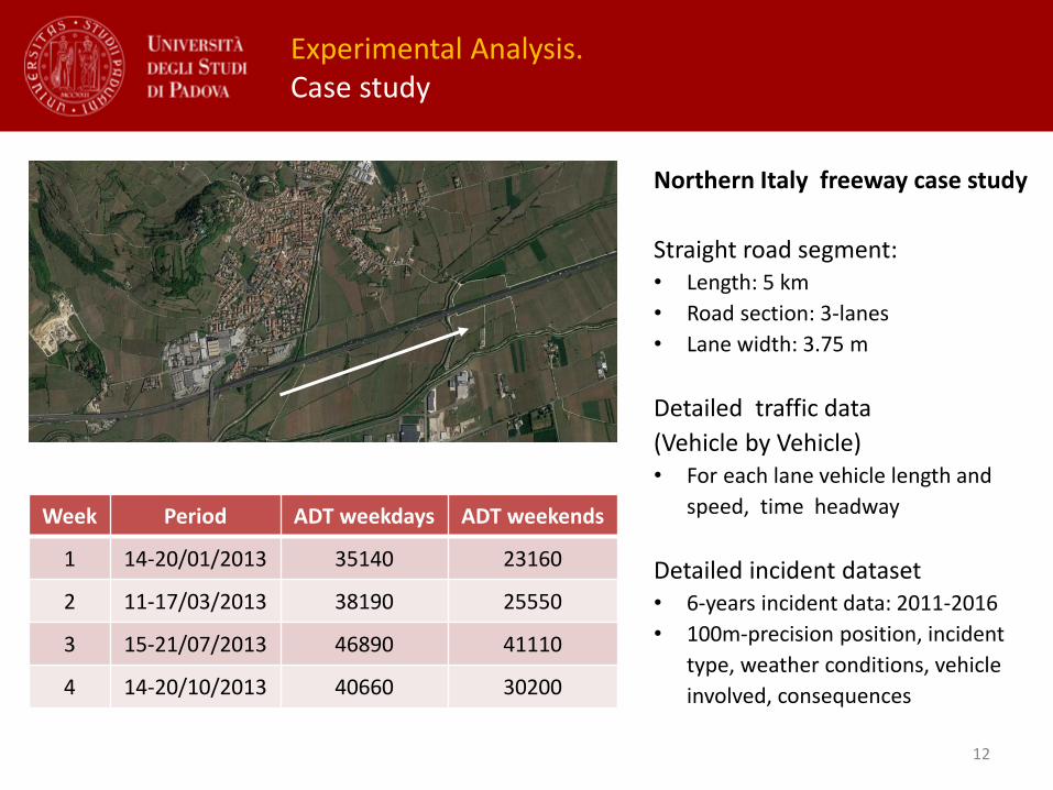
Experimental Analysis.Case study
Northern Italy freeway case study
Straight road segment:• Length: 5 km
• Road section: 3-lanes
• Lane width: 3.75 m
Detailed traffic data
(Vehicle by Vehicle)• For each lane vehicle length and
speed, time headway
Detailed incident dataset• 6-years incident data: 2011-2016
• 100m-precision position, incident
type, weather conditions, vehicle
involved, consequences
Week Period ADT weekdays ADT weekends
1 14-20/01/2013 35140 23160
2 11-17/03/2013 38190 25550
3 15-21/07/2013 46890 41110
4 14-20/10/2013 40660 30200

13
Experimental Analysis.Analysis of results
Block of maxima based on hourly values (BM-hour full)
DATA• Dataset contains the highest negated-TTC value for each hour block.• Only daytime hours considered (7:00 - 19:00).• Only working days considered (Monday - Friday).• 4 weeks data.60 maxima for each week, 240 in total.
CALIBRATION• Fitting the model to the whole dataset gives poor results. • Apparently, blocks are not large enough, and the dataset contains negated-TTC
values which are not really extremes.• The solution is to set a “limit value”. All data below it are not considered
extremes and are excluded from the dataset.
How to choose the limit value?
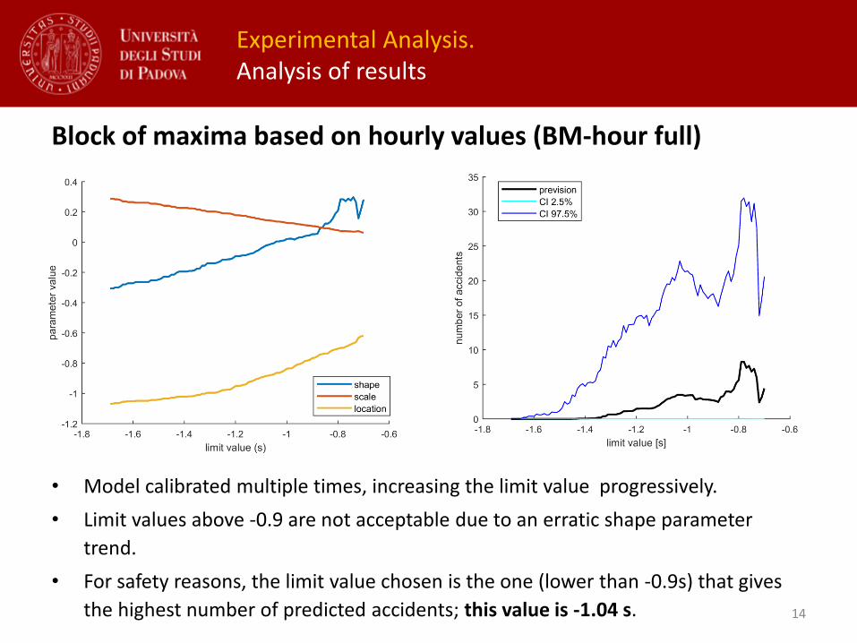
Block of maxima based on hourly values (BM-hour full)
• Model calibrated multiple times, increasing the limit value progressively.
• Limit values above -0.9 are not acceptable due to an erratic shape parameter
trend.
• For safety reasons, the limit value chosen is the one (lower than -0.9s) that gives
the highest number of predicted accidents; this value is -1.04 s. 14
Experimental Analysis.Analysis of results
15
Experimental Analysis.Analysis of results
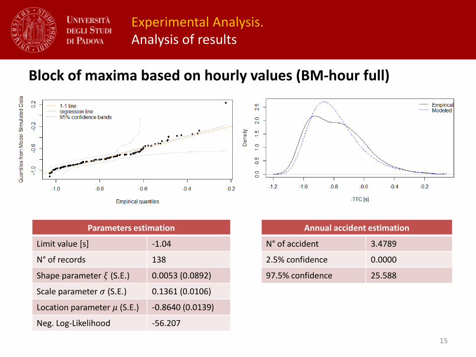
Block of maxima based on hourly values (BM-hour full)
Parameters estimation
Limit value [s] -1.04
N° of records 138
Shape parameter 𝜉 (S.E.) 0.0053 (0.0892)
Scale parameter 𝜎 (S.E.) 0.1361 (0.0106)
Location parameter 𝜇 (S.E.) -0.8640 (0.0139)
Neg. Log-Likelihood -56.207
Annual accident estimation
N° of accident 3.4789
2.5% confidence 0.0000
97.5% confidence 25.588
16
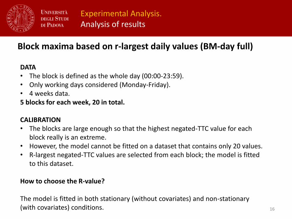
Experimental Analysis.Analysis of results
DATA• The block is defined as the whole day (00:00-23:59).• Only working days considered (Monday-Friday).• 4 weeks data.5 blocks for each week, 20 in total.
CALIBRATION• The blocks are large enough so that the highest negated-TTC value for each
block really is an extreme.• However, the model cannot be fitted on a dataset that contains only 20 values.• R-largest negated-TTC values are selected from each block; the model is fitted
to this dataset.
How to choose the R-value?
The model is fitted in both stationary (without covariates) and non-stationary (with covariates) conditions.
Block maxima based on r-largest daily values (BM-day full)

17
Experimental Analysis.Analysis of results
Block maxima based on r-largest daily values (BM-day full)
• Model calibrated multiple times, increasing the R-largest value progressively.
• Parameters show a regular trend with R higher than 20.
• Negative log-likelihood minimum when R is between 20 and 22.
• The selected R-largest value is 21; it also gives the highest number of predicted
accidents.
18
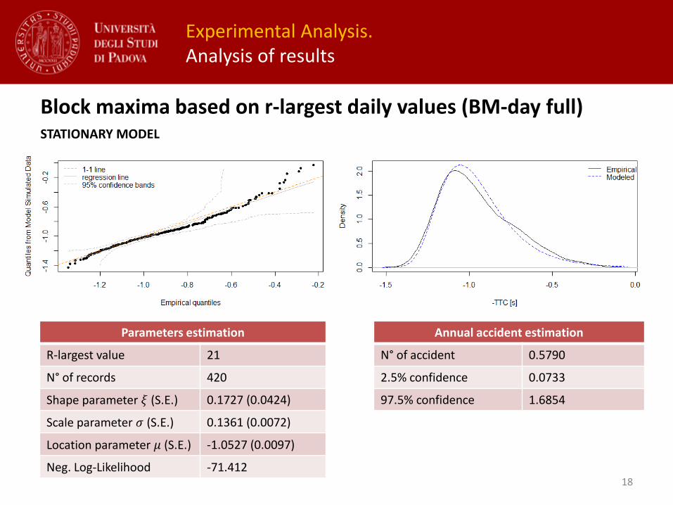
Experimental Analysis.Analysis of results
Parameters estimation
R-largest value 21
N° of records 420
Shape parameter 𝜉 (S.E.) 0.1727 (0.0424)
Scale parameter 𝜎 (S.E.) 0.1361 (0.0072)
Location parameter 𝜇 (S.E.) -1.0527 (0.0097)
Neg. Log-Likelihood -71.412
Annual accident estimation
N° of accident 0.5790
2.5% confidence 0.0733
97.5% confidence 1.6854
Block maxima based on r-largest daily values (BM-day full)STATIONARY MODEL

19
Experimental Analysis.Analysis of results
Parameters estimation
Shape parameter 𝜉 (S.E.) 0.0188 (0.0484)
Scale parameter 𝜎 (S.E.) 0.1696 (0.0072)
Location parameter 𝜇 (S.E.) -1.1943(0.0098)++3.54959(0.0000)*10-6*VOL
Neg. Log-Likelihood -75.89
Annual accident estimation
N° of accident 0.7058
2.5% confidence 0.0803
97.5% confidence 2.1826
The fitted non-stationary model was tested against the stationary model using the likelihood ratio test, resulting in a p-value of 0.0083, significantly smaller than alpha=0.05. R value is 21 in this case too (which results in 420 records).
Block maxima based on r-largest daily values (BM-day full)NON-STATIONARY MODEL - The model was fitted considering as a covariate the daily traffic volume
20
Experimental Analysis.Analysis of results
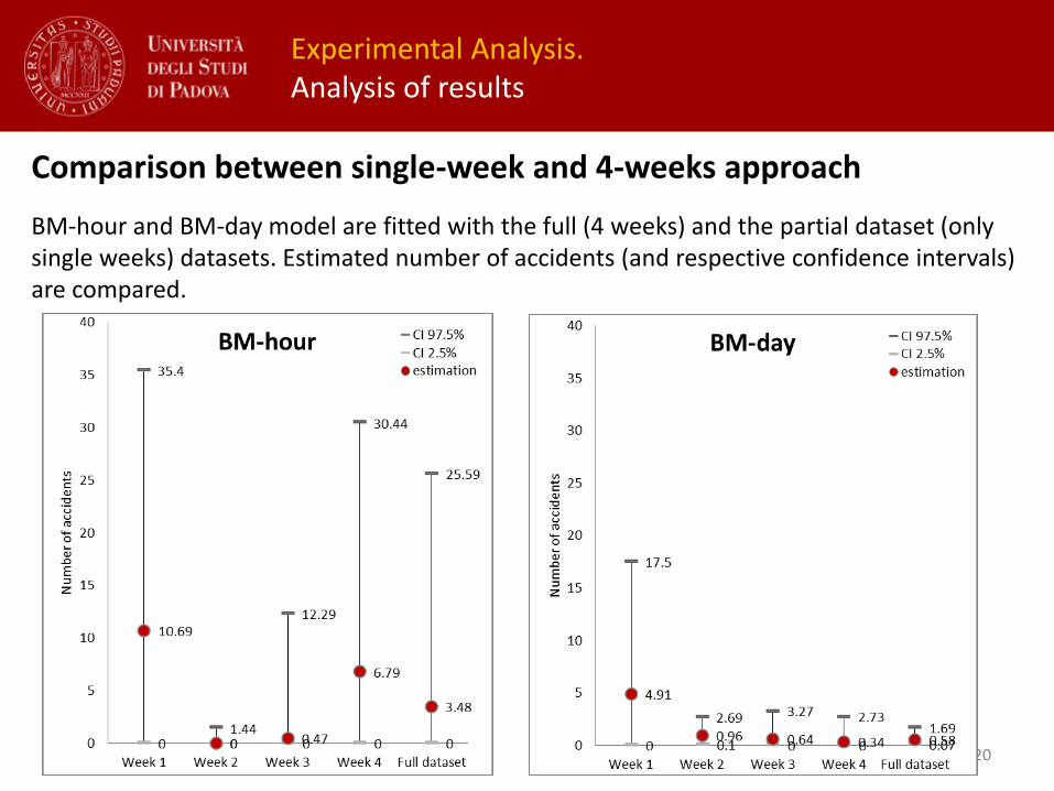
Comparison between single-week and 4-weeks approach
BM-hour and BM-day model are fitted with the full (4 weeks) and the partial dataset (only single weeks) datasets. Estimated number of accidents (and respective confidence intervals) are compared.

21
Experimental Analysis.Analysis of results
Comparison between predicted and observed accidents
• Accident data in the case-study road segment are available in the 2011-2016 period (six years).
• Only rear-end accidents that occurred on working days are considered.• The total number of observed accidents is 16; which is 2.67 observed accidents per
year.• Three of these accidents did not occur during the daytime (7:00-19:00): they
cannot be predicted with the BM-hour approach, which is fitted only with daytime data.
Model Predicted annual accidents [CI]
Annual mean of observed accidents [min;max]
BM-hour full 3.48 [0.00;25.8] 2.17 [1;3]
BM-day full (stationary) 0.58 [0.07;1.69] 2.67 [1;4]
BM-day full (non-stationary) 0.71 [0.08;2.18] 2.67 [1;4]

22
Experimental Analysis.Analysis of results
Comparison between predicted and observed accidents
The number of observed accidents depends on the distance from the section
What is the distance from the section inside which we can predict accidents?
Further tests will be carried out in different locations.

23
• Main concepts
• Focus of the paper
Introduction to FHWA Monitoring Factor Approach
• Characteristics of Clustering Methods
• Methodology of Study
• Analysis of Case Study Results
Clustering Methodsfor Road Grouping
• Concluding Remarks
• Future DevelopmentsConclusions

Conclusions.Concluding Remarks and Future Developments
24
This study proposes an Extreme Value Theory approach to estimate freeway rear-end collision risk for Italian freeways
The proposed BM approach (based on hourly and daily blocks) shows:
• overestimation of road accidents for BM-hour approach
• underestimation of road accidents for BM-day approach
• better performance using 4-weeks dataset for both approaches
• more precise estimates for BM-day approach
Future Research:
test the introduction of new covariates for the BM-day model
test Peak Over Threshold (POT) approach
apply the models to other road sections
apply the models to other types of accidents

25
Thank youfor your attention…