FREE VIBRATION OF 1-D AND 2-D SKELETAL STRUCTURES

A thesis submitted for the partial fulfillments of the requirements for degree of

Bachelor of Technology in “Civil Engineering”

By

Ashish Kumar Kanar

109ce0040

Under the guidance of

Prof. M.R. Barik

Department of Civil Engineering

NATIONAL INSTITUTE OF TECHNOLOGY

ROURKELA

(2013)

DEPARTMENT OF CIVIL ENGINEERING NATIONAL INSTITUTE OF TECHNOLOGY,ROURKELA

ODISHA, INDIA-769008

CERTIFICATE This is to certify that the thesis named, “Free Vibration of 1-D and 2-D Skeletal Structures,” submitted by Ashish Kumar Kanar (B.Tech:109CE0040) in partial fulfillment of the requirements for the award of Bachelor of Technology in Civil Engineering during session 2012-2013 at National Institute of Technology, Rourkela is a bonafide record of research work carried out by him under my supervision and guidance. The candidate has fulfilled all the prescribed requirements. The thesis which is based on candidates‟ own work has not been submitted elsewhere for a degree/diploma. In my opinion, the thesis is of standard required for the award of a Bachelor of Technology degree in Civil Engineering. Place: Prof. M.R. Barik Dept. of Civil Engineering Associate Professor National Institute of Technology

ACKNOWLEDGEMENTS

On the submission of my thesis named, “Free Vibration of 1-D and 2-D Skeletal Structures” I would like to express my honest gratitude to my project guide Prof. M.R. Barik (Associate Prof. in Civil Engineering Department) for his support and inspiration during my project work in the last one year. I truly acknowledge and value his motivation and guidance from the beginning to end of my project work which would be remembered for ever.

I am also very thankful to Prof. Ramakar Jha (our Faculty advisor) for his priceless guidance and suggestions during this project period.

I am also thankful to our branch professors for providing solid background for my knowledge and research thereafter. They have been a great source of knowledge and motivation for the last 4yr. without whom this thesis can’t be imagined and I thank them from the bottom of my heart.

At last, but not the least I would like to thank the staff of Civil Engineering Department for their constant help and support and providing place to work during the whole project period. I would also like to thank my friends for providing proper environment for my research work.

ASHISH KUMAR KANAR

109CE0040

B.TECH (CIVIL ENGINEERING)

ABSTRACT

A structure is to be designed to achieve a definite set of natural frequencies to avoid resonance,

to decrease dynamic stresses, or to provide study materials for certain critical computation of

vibration instrumentation. Structures vibrate constantly in certain frequencies under dynamic

loadings. So, it is necessary to undertake vibration analysis to avoid resonance with the natural

frequency. The natural frequency depends upon stiffness and mass distributions, boundary

conditions and the modes in which they are excited. This project “Free Vibrations of 1-D and 2-

D Skeletal Structures,” aims in computing the free natural frequencies of 1-D and 2-D skeletal

structures. FEM (finite Element Analysis) is a versatile numerical technique which is quite

effective for vibrational analysis of structures which are under dynamic loads. MATLAB codes

are developed using FEM techniques in which inertia and stiffness matrices are constructed.

Finally the natural frequencies are computed.

INDEX

Sl. No CHAPTER PAGE NO

1. INTRODUCTION 1-2

2. LITERATURE REVIEW 3-4

3. FEM FORMULATION 5-34

OF PROBLEM

4. RESULTS 34-44

5. CONCLUSION AND DISCUSSION 45-47

6. REFERENCES 48-49

LIST OF TABLES

Table 1 Title Page no. 1 Natural frequencies of a bar 35

2 Natural frequencies of beam 37

3 Natural frequencies of portal frame 38

4 Natural frequencies of stepped beam 40-41

5 Natural frequencies of stepped circular beam with various

boundary conditions having varying step ratios

42-43

.LIST OF FIGURES

Figures Title of figure Page no.

Figure 1 A 1-D rod 12

Figure 2 A planar truss element 14

Figure 3 A plane frame 23

Figure 4 A plane frame element with local and global co-ordinates 24

Figure 5 Stepped beam 26

Figure 6 Clamped-free boundary condition of stepped beam 28

Figure 7 Free-slide boundary condition of stepped beam 28

Figure 8 Free-pinned boundary condition of stepped beam 29

Figure 9 Pinned-pinned boundary condition of stepped beam 30

Figure 10 Clamped – pinned boundary condition of stepped beam 30

Figure 11 Clamped – clamped boundary condition of stepped beam 31

Figure 12 Clamped – slide boundary condition of stepped beam 32

Figure 13 Slide – pinned boundary condition of stepped beam 32

Figure 14 Slide – slide boundary condition of stepped beam 33

Figure 15 cantilever bar 35

Figure 16 truss structure 36

Figure 17 unit beam 37

Figure 18 Portal frame 38

Figure 19 Stepped beam 39

Figure 20 Graph of natural frequencies vs step ratios for various boundary conditions

44

Chapter - 1

INTRODUCTION

1

If a body is moving in a oscillating or reciprocating manner, it is called vibration if it involves

deformation of body. However if, the reciprocating motion involves only the rigid body

movement without involving its deformation, then it is termed as oscillation. The movement of a

pendulum is simple harmonic and so is for a ship (if considered as a rigid body) moving over the

waves. Unwanted vibration can cause degradation in performance of the structure. The aim of

vibrational analysis of a structure is to suppress unwanted vibrations, to generate desirable

vibrations, to control or modify it and its isolation to minimize the structural response.

When the excitation force (the driving factor for the initiation of vibration) in a structure doesn’t

play any role after initiation of motion; then it is called free vibration. The corresponding

frequencies are called natural frequencies of vibration. Among them the lower natural

frequenciesare of optimum consideration in the vibrational analysis of a structure.

There are two ways to solve vibration problems.

i. Analytical method

ii. Numerical method

Analytical methods give accurate results but they require symmetry and simplicity of the

problem under consideration whereas numerical techniques give approximate results but these

are meant for complex problems and time efficient. FEM (finite element method) is one of the

most flexible and effective numerical tool for the analysis of vibration of a system.

In this thesis, free vibration of the following structures has been considered.

i. Free torsional vibration of shaft

ii. Free axial vibration of rod

iii. Free vibration of truss

iv. Free vibration of Bernoulli-Euler beam

v. Free vibration of Timoshenko beam

vi. Free vibration of plane frame

vii. Free vibration of stepped beam

2

Chapter - 2

LITERATURE REVIEW

3

Young W. Kwon and Hyochoong Bang,[1] in their book, “Finite Element Method using

MATLAB,” analyzed free vibration of trusses, both Euler and Timoshenko beams, and frame

structures to get their natural frequencies using FEM . They compared the FEM results of natural

frequencies with the results of analytical methods.

M. Asghar Bhatti,[2] in his book, strived to explain and teach the mechanical aspects of the

finite element method and give satisfactory explanations for theoretical questions related to

truss, beams and frames.

S.K. Jang and C.W. Bert,[3] in their paper, analyzed the free vibration of stepped beam. In their

study, the lowest natural frequency of a stepped beam with two different cross sections was

sought for various boundary conditions. Exact solutions had been calculated and are compared

with the results obtained by the use of FEM with non-polynomial shape functions and with a

commercial code,MSC/pal.

R.D. Blevin’s[4] paper was quite helpful in understanding the basics of natural frequency and

mode shapes, which are two essential terms in vibration analysis.

T.S. Balasubramanian and G. Subramanian,[5],[6] in their paper compared the frequency

values obtained by using 2DPN(degree-per-node) elements and 4DPN elements for uniform,

stepped and continuous beams for various boundary conditions to show the superior performance

of the 4DPN element. They also studied the beneficial effects of steps on the free vibration

response of stepped beams.

Larisse Klein[8] in 1974, is his paper, analyzed the free vibration of elastic beams with non-

uniform characteristics by a new method which was seen to combine the advantages of finite

element method and Rayleigh-Ritz analysis.

G.M.L. Gladwell[9](Institute of Sound and Vibration Research, University of Southampton,

England), in his paper, determined the natural frequencies and principal modes of un-damped

free vibration of a plane frame composed of a rectangular grid of uniform beams.

4

Chapter – 3

FEM FORMULATION OF

THE PROBLEM

5

FINITE ELEMENT METHOD :

FEM is a flexible approximate numerical technique for solving partial differential equations

which is originated from complex elasticity and structural problems. FEM allows for detailed

visualization of stress and strains inside the body of a structure. Any domain/continuum is

considered as an assemblage of number of pieces having very small dimensions called finite

elements. These elements are connected through a number of joints called nodes.

Every physical problemisanalyzed/computed by simplifying certain assumptions. Hence the true

behavior of structure should be observed within these constraints and certain errors creep into the

engineering computations.

The following procedure is performed for FEM.

i. Discretization of the domain

ii. Identification of variables(unknown displacement at each nodes)

iii. Choice of approximating functions

iv. Generation of element stiffness matrix

v. Generation of overall stiffness matrix

vi. Formation of element inertia matrix

vii. Formation of overall inertia matrix

viii. Application of boundary conditions

ix. Solution of simultaneous equations

6

Vibration analysis of structures comprises of two parts:

a) Static analysis

b) Dynamic analysis

In static analysis formation of global stiffness matrix and global inertia matrix are executed.

In dynamic analysis, computation of natural frequencies is executed.

According to Newton’s law,

F=ma

And, kx=ma

Hence, kx=ma

=>kx-ma=0

=> kx- ω2mx=0 (since x=asin ωt)

=> (K- ω2m) x=0

Since x cannot be zero,hence, in matrix form

[K]-ω2[M]=0

Square root of the diagonal elements of the eigen vector will give the values of natural

frequencies of the system.

7

FREE TORSIONAL VIBRATION OF SHAFT :

Let us consider an un-damped free vibration case.

Torsional vibration is nothing but the twisting effect of the ends of a shaft.

A shaft has 2 nodes at its ends.

Let, the displacements at the two ends are ϕ1 and ϕ2.

ϕ1 and ϕ2 are nothing but the angle of twist.

Let ϕ1=α1,

ϕ2=α1+ L*α2

At any point along the shaft, ϕ= α1 +xα2 ; which is twist at x distance from node1

We can write,

ϕ= <1 x > {α1 α2 }T ………….eq(1)

Linear interpolation function can be taken as,

{ ϕ1 ϕ2 }T=[1 0; 1 L]{α1 α2 }T

Or, {α1 α2 }T = [1 0; 1 L ]-1{ ϕ1 ϕ2 }T

Or, {α1 α2 }T = (1/L) [L 0 ; -1 1 ]{ϕ1 ϕ2 }T

Putting this value in eq1, we get

Φ= <1 x > (1/L) [L 0; -1 1]{ϕ1 ϕ2 }T

=< (1-x/L), x/L > { ϕ1, ϕ2}T

Or,

8

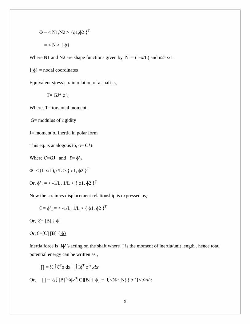
Φ = < N1,N2 > {ϕ1,ϕ2 }T

= < N > { ϕ}

Where N1 and N2 are shape functions given by N1= (1-x/L) and n2=x/L

{ ϕ} = nodal coordinates

Equivalent stress-strain relation of a shaft is,

T= GJ* ϕ’x

Where, T= torsional moment

G= modulus of rigidity

J= moment of inertia in polar form

This eq. is analogous to, σ= C*Ɛ

Where C=GJ and Ɛ= ϕ’x

Φ=< (1-x/L),x/L > { ϕ1, ϕ2 }T

Or, ϕ’x = < -1/L, 1/L > { ϕ1, ϕ2 }T

Now the strain vs displacement relationship is expressed as,

Ɛ = ϕ’x = < -1/L, 1/L > { ϕ1, ϕ2 }T

Or, Ɛ= [B] { ϕ}

Or, Ɛ=[C] [B] { ϕ}

Inertia force is Iϕ’’x acting on the shaft where I is the moment of inertia/unit length . hence total

potential energy can be written as ,

∏ = ½ ∫ ƐTσ dx + ∫ IϕT ϕ’’x𝑑𝑥

Or, ∏ = ½ ∫ [B]T<ϕ>T[C][B] { ϕ} + I∫<N>{N}{ ϕ’’}<ϕ>𝑑𝑥

9

Or, ∏ = (<ϕ>T/2) (∫[B]T [C][B]𝑑𝑥 ) { ϕ} + I{ ϕ}∫<N>{N}{ ϕ’’}𝑑𝑥

The principle of minimum potential energy requires,

∏’{ϕ} = 0

i.e. (∫BTCB𝑑𝑥) + I (∫NTN𝑑𝑥){ϕ’’} ={0}

this is equivalent to.

[K]e{ ϕ}e + [M]e{ ϕ’’}e ={0}

Where,

[K]e = (∫BTCB𝑑𝑥)

= ∫ < -1/L, 1/L>TGJ< -1/L, 1/L >𝑑𝑥

= GJL [1/L2-1/L2; -1/L2 1/L2]

= (GJ/L)[1,-1 ; -1,1 ]

And [M]e = I∫<(1-x/L), x/L>T<(1-x/L),x/L>𝑑𝑥

= (IL/6) [2, 1; 1, 2]

If [M]e is a lumped mass matrix (it is assumed that mass is lumped at nodes ), then

[M]e= (IL/2)[1, 0; 0,1]

Though consistent mass is less erroneous, the lumped mass gives better results because both

stiffness and mass are overestimated, thus resulting in correcting in correct answer.

When all elements of the element stiffness matrices and mass matrices are assembled and

boundary conditions incorporated, the final eq. of vibration is

10

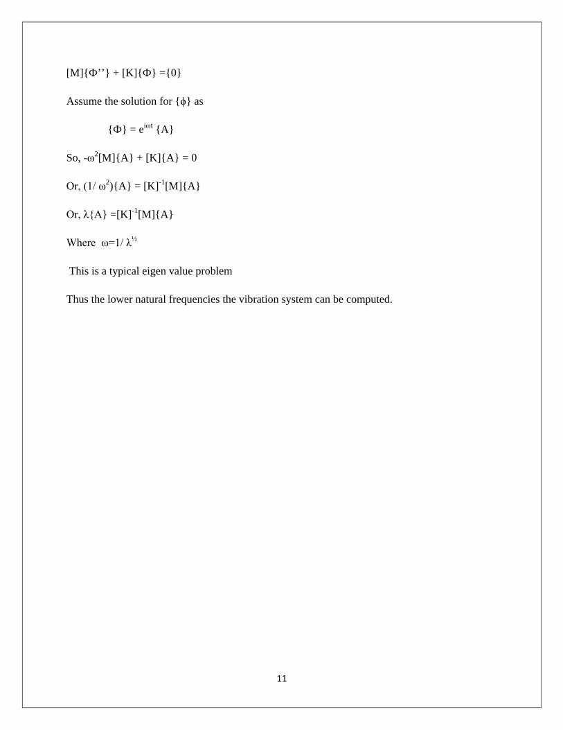
[M]{Ф’’} + [K]{Ф} ={0}

Assume the solution for {ϕ} as

{Ф} = eiωt {A}

So, -ω2[M]{A} + [K]{A} = 0

Or, (1/ ω2){A} = [K]-1[M]{A}

Or, λ{A} =[K]-1[M]{A}

Where ω=1/ λ½

This is a typical eigen value problem

Thus the lower natural frequencies the vibration system can be computed.

11

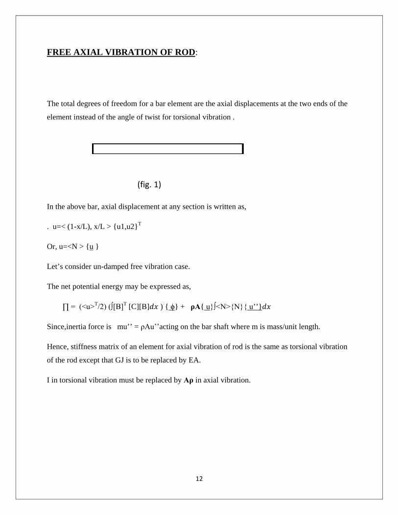
FREE AXIAL VIBRATION OF ROD:

The total degrees of freedom for a bar element are the axial displacements at the two ends of the

element instead of the angle of twist for torsional vibration .

(fig. 1)

In the above bar, axial displacement at any section is written as,

. u=< (1-x/L), x/L > {u1,u2}T

Or, u=<N > {u }

Let’s consider un-damped free vibration case.

The net potential energy may be expressed as,

∏ = (<u>T/2) (∫[B]T [C][B]𝑑𝑥 ) { ϕ} + ρA{ u}∫<N>{N}{ u’’}𝑑𝑥

Since,inertia force is mu’’ = ρAu’’acting on the bar shaft where m is mass/unit length.

Hence, stiffness matrix of an element for axial vibration of rod is the same as torsional vibration

of the rod except that GJ is to be replaced by EA.

I in torsional vibration must be replaced by Aρ in axial vibration.

12

Hence, [K]e = (EA/L)[1,-1 ; -1,1]

And, [M]e= Aρ∫<(1-x/L),x/L>T<(1-x/L),x/L>𝑑𝑥

Thus, when all elements of all the element stiffness and element inertia matrices are assembled

and boundary conditions incorporated, the final eq. of free vibration is solved to find the natural

frequencies.

Mu’’ + Ku = 0

Assume the solution for {ϕ} as

{u} = eiωt {A}

So, -ω2[M]{A} + [K]{A} = 0

Or, (1/ ω2){A} = [K]-1[M]{A}

Or, λ{A} = [K]-1[M]{A}

Where ω=1/ λ½

This is a typical eigen value problem

Thus we can find the lowest natural frequency of the vibration system.

13

FREE VIBRATION OF PLANAR TRUSS:

Consider a truss element oriented as shown in the global coordinate system

(fig.2)

Since the truss elements are only subjected to axial forces,

{Fzi,Fzj}T= EA/L[1,-1 ; -1,1]{wi,wj}T

The local displacement < wi,wj > can be written as in terms of global coordinates.

{wi,wj}T = [c,s,0,0 ; 0,0,c,s ][ui,vi,uj,vj ]T …….eq1

Where c=cosαand s=sinα

wi=uicosα+visinα

wj= ujcosα+vjsinα

Eq1 can be written as,

{q}1=[T]{q}g

Where {q}l=local displacement

14

{q}g=global displacement

Since F=Kq

Hence, {F}g= [T]T{F}l

Or, {F}g = [T]T{K}l{q}l

Or, {F}g = [T]T{K}l[T]{q}g

Or, {F}g= [K]g{q}g

Where,

[K]g=[T]T{K}l[T]

= [c,s,0,0 ; 0,0,c,s ]T(EA/L)[1,-1 ; -1,1] [c,s,0,0 ; 0,0,c,s ]

= (EA/L)[c2 cs -c2 -cs ; cs s2 -cs -s2 ; - c2 -cs cs ; -cs -s2 cs s2]

Mass matrix in global system,

[M]g = ρAL/6[2 0 1 0 ; 0 2 0 1 ; 1 0 2 0 ; 0 1 0 2 ]

Then the dynamic equation,

[K]g - ω2[M]g= 0

Solving this equation and by finding the square root of diagonal elements of the eigen vector we

can determine the natural frequencies.

15

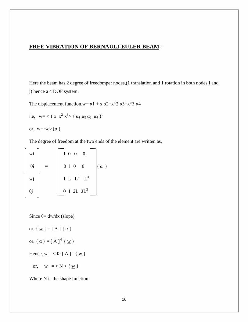
FREE VIBRATION OF BERNAULI-EULER BEAM :

Here the beam has 2 degree of freedomper nodes,(1 translation and 1 rotation in both nodes I and

j) hence a 4 DOF system.

The displacement function,w= α1 + x α2+x^2 α3+x^3 α4

i.e, w= < 1 x x2 x3> { α1 α2 α3 α4 }t

or, w= <d>{α }

The degree of freedom at the two ends of the element are written as,

wi 1 0 0. 0.

θi = 0 1 0 0 { α }

wj 1 L L2 L3

θj 0 1 2L 3L2

Since θ= dw/dx (slope)

or, { w } = [ A ] { α }

or, { α } = [ A ]-1 { w }

Hence, w = <d> [ A ]-1 { w }

or, w = < N > { w }

Where N is the shape function.

16

N1 = (1- 3x2/L2 + 2x3/L3),

N2 = (x - 2x2/L + x3/L2),

N3 = (3x2/L2 – 2 x3/L3),

N4 = (-3 x2/L + x3/L2 )

Strain enegy, U = EI/2 ∫ (d2w/dx2 )2dx

= EI/2 <w > ∫ {Nxx} < Nxx > dx { w }

Or, dU/dx = [K] { w } (since U=1/2 kx2 and dU/dx= kx )

Hence, [K] = EI ∫ {Nxx} < Nxx > dx

Where,{Nxx}t = < ( -6/ L2 +12x/ L3 ), (-4/L+6x/ L2 ), (6/ L2 -12x/L ), (-2/L +6x/ L2 )>

So, element stiffness matrix is given by,

12 6L -12 6L

[K]e = EI/L3 6L 4L2-6L 2L2

-12 -6L 12 -6L

6L 2*L2 -6*L 4*L2

Kinetic energy, T = w2 /2 ∫ ρA w2dx

Or, T = w2ρA/2<w > ∫ {N} < N> dx

= ω2[M]

Where [M] = ρA ∫ {N} < N> dx

17

So, 156 22L 54 -13L

22L 4L2 13L -3 L2

[M] = ρAL/42054 13L 156 -22L

-13L -3 L2 -22L 4 L2

Thus, when the elements of all element stiffness and inertia matrices of every nodes are

assembled followed by incorporation of boundary conditions, the final eq. of free vibration is

solved to get the natural frequencies.

Mu’’ + Ku = 0

Assume the solution for {ϕ} as

{u} = eiωt {A}

So, -ω2[M]{A} + [K]{A} = 0

Or, (1/ ω2){A} = [K]-1[M]{A}

Or, λ{A}=[K]-1[M]{A}

Where ω=1/ λ½

This is a typical eigen value problem

Thus we can find the lowest natural frequency of the vibration system .

18

FREE VIBRATION OF TIMOSHENKO BEAM :

Timoshenko beams are deep beams .with the increasing depth of beam, the effect of transverse shear deformation and rotary inertia become more important.

The deflection function is given by \,

w= < 1 x x2 x3> { α1 α2 α3 α4 }t

the relation between transverse shear strain ϒ, w’ and θ is

w’= ϒ + θ

where θ denotes the slope deflection curve due to bending deflection alone.

Transverse shear strain may be taken as a constant independent of x,

ϒ = βo(assumed)

Moment curvature relationship is given by,

M = -EI dθ/dx

Shear force V is related to transverse shear strain by,

V = KAG ϒ

Where, K = Timoshenko’s shear constant

= 5/6 (rectangular section)

= 9/10 (circular section)

Bending moment and shear force are related as follows .

V = dM/dx

19

we know, w’ = θ + ϒ

or, θ = w’- ϒ

w = α1 +α2x + α3x2 + α4x3

or, w’= α2 + 2x α3 +3x2 α4

or, w’’ = 2α3 +6x α4

or, w’’’ = 6 α4

we have

dθ/dx = w’’

or, d2θ/dx2 = w’’’

we know that

V = dM/dx = -EI d2θ/dx2

Or, KAG ϒ = -EI* 6 α4

Or, ϒ = -6EIα4/ KAG

Or, β0 = - α4ϕL2/2 (where ϕ =12EI/KAGL2 )

Substituting the values we get nodal displacement as,

wi 1 0 0 0

θi = 1 0 - ϕL2/2 0 { α }

wj 1 L L2 L3

θj 1 2L (3-ϕ/2)L2 0

{q} = [A]{ α }

Or, { α } = [A]-1{q}

20

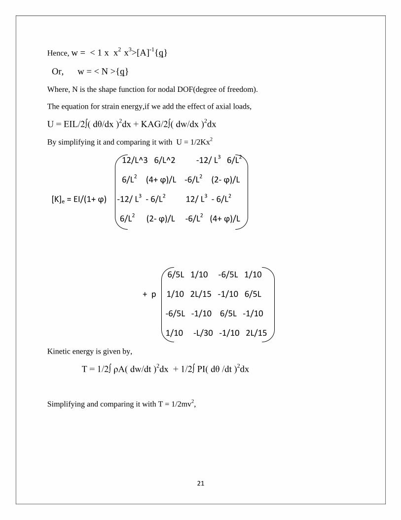
Hence, w = < 1 x x2 x3>[A]-1{q}

Or, w = < N >{q}

Where, N is the shape function for nodal DOF(degree of freedom).

The equation for strain energy,if we add the effect of axial loads,

U = EIL/2∫( dθ/dx )2dx + KAG/2∫( dw/dx )2dx

By simplifying it and comparing it with U = 1/2Kx2

12/L^3 6/L^2 -12/ L3 6/L2

6/L2 (4+ ϕ)/L -6/L2 (2- ϕ)/L

[K]e = EI/(1+ ϕ) -12/ L3 - 6/L2 12/ L3 - 6/L2

6/L2 (2- ϕ)/L -6/L2 (4+ ϕ)/L

6/5L 1/10 -6/5L 1/10

+ p 1/10 2L/15 -1/10 6/5L

-6/5L -1/10 6/5L -1/10

1/10 -L/30 -1/10 2L/15

Kinetic energy is given by,

T = 1/2∫ ρA( dw/dt )2dx + 1/2∫ PI( dθ /dt )2dx

Simplifying and comparing it with T = 1/2mv2,

21

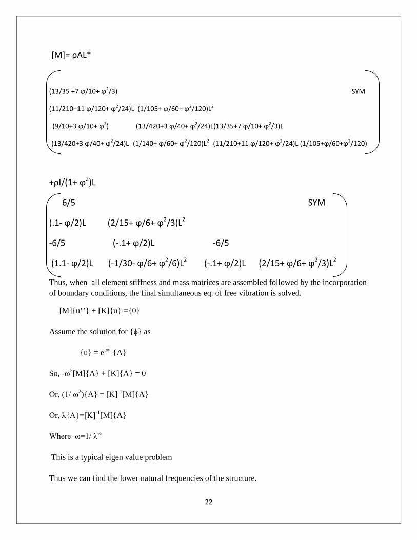
[M]= ρAL*

(13/35 +7 ϕ/10+ ϕ2/3) SYM

(11/210+11 ϕ/120+ ϕ2/24)L (1/105+ ϕ/60+ ϕ2/120)L2

(9/10+3 ϕ/10+ ϕ2) (13/420+3 ϕ/40+ ϕ2/24)L(13/35+7 ϕ/10+ ϕ2/3)L

-(13/420+3 ϕ/40+ ϕ2/24)L -(1/140+ ϕ/60+ ϕ2/120)L2 -(11/210+11 ϕ/120+ ϕ2/24)L (1/105+ϕ/60+ϕ2/120)

+ρI/(1+ ϕ2)L

6/5 SYM

(.1- ϕ/2)L (2/15+ ϕ/6+ ϕ2/3)L2

-6/5 (-.1+ ϕ/2)L -6/5

(1.1- ϕ/2)L (-1/30- ϕ/6+ ϕ2/6)L2 (-.1+ ϕ/2)L (2/15+ ϕ/6+ ϕ2/3)L2

Thus, when all element stiffness and mass matrices are assembled followed by the incorporation of boundary conditions, the final simultaneous eq. of free vibration is solved.

[M]{u’’} + [K]{u} ={0}

Assume the solution for {ϕ} as

{u} = eiωt {A}

So, -ω2[M]{A} + [K]{A} = 0

Or, (1/ ω2){A} = [K]-1[M]{A}

Or, λ{A}=[K]-1[M]{A}

Where ω=1/ λ½

This is a typical eigen value problem

Thus we can find the lower natural frequencies of the structure.

22

FREE VIBRATION OF PLANE FRAME

Consider a plane framework as the one shown in figure.

(figure 3)

This plane frame is vibrating in its own plane. When applying finite element method to such structures,the following procedures should be used.

1. Divide each member into appropriate no of elements. 2. Derive the energy expressions for each element in terms of nodal degrees of freedom

relative to a local seta of axes. 3. Transform the energy expressions for each element into expressions involving nodal

degrees of freedom relative to a common set of global axes. 4. Add the energies of the elements together.

The kinetic energy,

Te = 1/2 ∫ ρA(u’2 +v’2)dx

The potential energy,

Ue = ∫ EA(du/dx)2dx +1/2∫ EIz(d2v/dx2)2dx

23

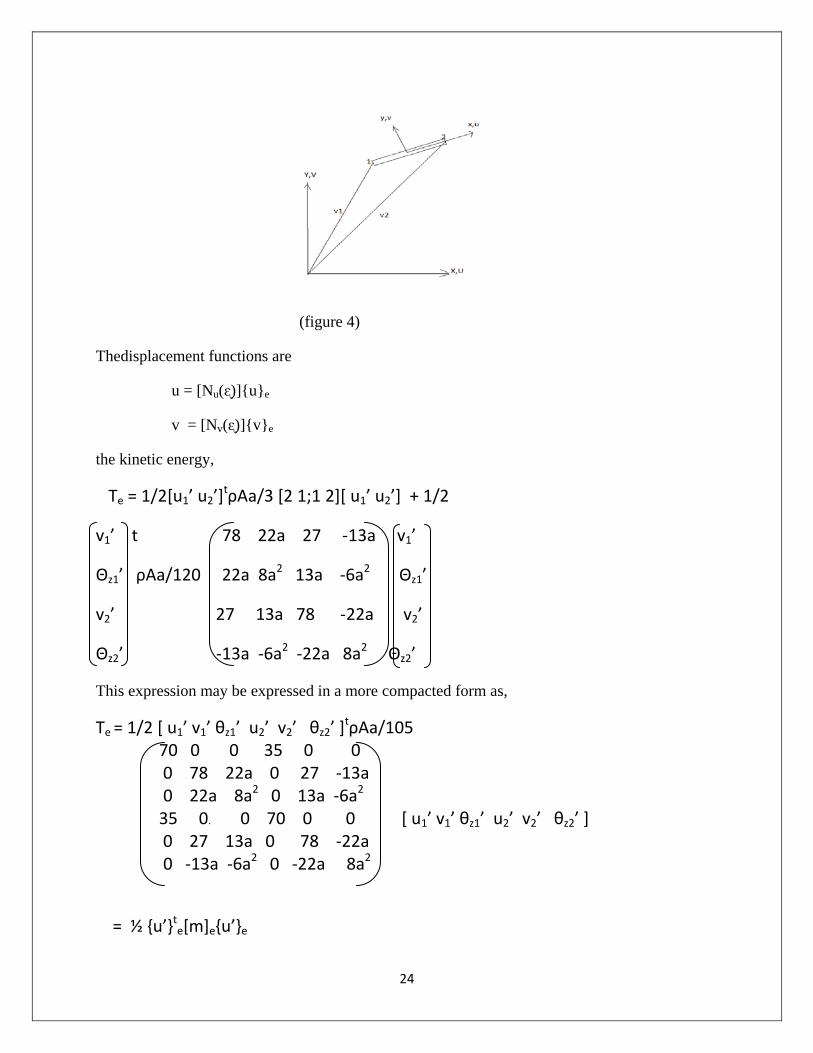
(figure 4)

Thedisplacement functions are

u = [Nu(ᶓ)]{u}e

v = [Nv(ᶓ)]{v}e

the kinetic energy,

Te = 1/2[u1’ u2’]tρAa/3 [2 1;1 2][ u1’ u2’] + 1/2

v1’ t 78 22a 27 -13a v1’

Θz1’ ρAa/120 22a 8a2 13a -6a2 Θz1’

v2’ 27 13a 78 -22a v2’

Θz2’ -13a -6a2 -22a 8a2 Θz2’

This expression may be expressed in a more compacted form as,

Te = 1/2 [ u1’ v1’ θz1’ u2’ v2’ θz2’ ]tρAa/105 70 0 0 35 0 0 0 78 22a 0 27 -13a 0 22a 8a2 0 13a -6a2 35 0. 0 70. 0 0 [ u1’ v1’ θz1’ u2’ v2’ θz2’ ] 0 27 13a 0 78 -22a 0 -13a -6a2 0 -22a 8a2

= ½ {u’}te[m]e{u’}e

24

So, [m]e = 70 0 0 35 0 0 0 78 22a 0 27 -13a 0 22a 8a2 0 13a -6a2 ρAa/105 35 0 0 70 0 0

0 27 13a 0 78 -22a

0 -13a -6a20 -22a 8a2

Substituting the displacement function into strain energy function we get

U = 1/2{u}te[k]e{u}e

Where, [k]e =

(a/rz)2 0 0 - (a/rz)2 0 0 0 3.. 3a 0 -3 3a 0 3a 4a2 0 -3a 2a2 EIz/2a3 - (a/rz)2 0 (a/rz)2 0 0

0 -3 00 3 -3a 0

0 3*a 2a2 0 -3a 4a2

Thus, when all element stiffness and inertia matrices of each node are assembled and boundary conditions incorporated, the final eq. of free vibration is solved.

[k]- ω2[M] = 0

Square root of the diagonal elements of the eigen vector will give the values of natural frequencies of the system.

25

FREE VIBRATION OF STEPPED BEAM :

(figure 5)

Where,

A1= area of 1st beam section

A2 = area of 1st beam section

I1= moment of inertia of 1st beam section

I1= moment of inertia of 2nd beam section

L1= length of 1st beam section

L2 = length of 2nd beam section

Ρ = unit weight of beam material

A2 =αA1 and I=I2/I1

I =α2 and L1= L2=2a=L/2

Assume degree of freedom per node = 2

26

Now, inertia matrix of 1st beam element is given by,

[M]1= ρA1a/105

−−

8a^222a-6a^2-13a-22a-7813a27a^2613a^2822

13272278aa

aa

similarly, inertia matrix of 1st beam element is given by,

[M]2= ρ(I1)A1a/105

−−

8a^222a-6a^2-13a-22a-7813a27a^2613a^2822

13272278aa

aa

Inertia mass of the stepped beam,

[M]=ρA1a/105

−−−−

−+−−−

−−+−−

IaIaIaIaIaIIaIIaIaIaIaaa

IaIIaIaaaaa

aa

2^8222^613002278132700

2^613)1(2^8)1(222^6131327)1(22)1(781327

002^6132^8220013272278

Stiffness matrix of 1st beam element,

[K]1 = EI1/(2a3)

−−

4a^23a-2a^23a3a-33a-3-a^223a^2433333

aaaa

Stiffness matrix of 2nd beam element,

[K]2= EI*I1/(2a3)

−−

4a^23a-2a^23a3a-33a-3-a^223a^2433333

aaaa

Now the stiffness matrix of the stepped beam is given by;

[K] =EI1/(2a3)

−−−−

−+−−−+−−

−−

IaaIIaaIaIIaII

IaaIIaIaaaaIIIaIa

aaaaaa

)2^(43)2^(2300333300

)2^(23)1)(2^(4)1(32^2333)1(3)1(333

002^232^43003333

27

- : BOUNDARY CONDITIONS:-

We have to find out [M] and [K] matrices for the above stepped beam for different boundary conditions.

1) C-F (clamped –free) :-

In this case x1, θ1 =0 (figure 6)

Hence we eliminate col(1),col(2),row(1),row(2) from [K] and [M] to find the respective matrices in C-F condition.

Inertia matrix,

[M]C-F = ρA1a/105

−−−−

−+−

−−+

IaIaIaIaIaIIaI

IaIaIaIaIaIIaI

)2^(822)2^(61322781327

)2^(613)1)(2^(8)1(221327)1(22)1(78

Stiffness matrix,

[K]C-F= EI1/2a3

−−−−

−+−−−+

IaaIIaaIaIIaII

IaaIIaIaaIIIaI

)2^(43)2^(233333

)2^(23)1)(2^(4)1(1333)1(3)1(3

2)F-S (free- slide) :-

In this case, θ2 =0

Hence eliminate col(6) and row(6) from the general [M],[K] to obtain the corresponding matrices for F-S b condition. (figure 7)

28

Inertia matrix,

[M]F-S=ρA1a/1055

+−−−

−+

−−

IIaI

IaIaIaaa

IIaIa

aaaaaa

78132700

13)1(2^8)1(222^613

27)1(22)1(781327

02^6132^822013272278

Stiffness matrix,

[K]F-S=EI1/(2a3)

−−

−+−

−−+−−

−

−

IaII

aIIaIaaa

IIaIa

aaaa

aa

33300

3)1)(2^(4)1(32^23

3)1(3)1(333

02^232^43

03333

3)F-P(free-pinned) :-

In this boundary condition, x2 =0

Hence eliminate col(5) and row(5) from the general [M],[K] to obtain the corresponding matrices for F-P boundary condition. (figure 8)

Inertia matrix,[M]F-P= ρA1a/105

−−

−+−−−

−−+

−

−

IaIaIa

IaIaIaaa

IaIaIa

aaaa

aa

2^82^61300

2^6)1(2^8)1(222^613

13)1(22)1(781327

02^6132^822

013272278

Stiffness matrix,

. [K] F-P=EI1/(2a3)

+−

−+−−

−

−

IaIaaI

IaIaIaaa

aIIaIa

aaaa

aa

)2^(4)2^(2300

)2^(2)1)(2^(4)1(32^23

3)1(3)1(333

02^232^43

3333 0

29

4) P-P(pinned-pinned) :-

In this case, x1, x2=0

Hence eliminate row(1),col(1),col(5) and row(5) from the general [M],[K] to obtain the corresponding matrices for P-P case. (figure 9)

Inertia matrix,

[M]P-P=ρA1a/105

−−

−+−−

−−+

−

IaIaIa

IaIaIaa

IaIaIa

aaa

2^82^6130

2^6)1(2^8)1(222^6

13)1(22)1(7813

02^6132^8

Stiffness matrix,

[K]P-P= EI1/(2a3)

+−−+−

−

IaIaaIIaIaIaa

aIIaIaaaa

)2^(4)2^(230)2^(2)1)(2^(4)1(32^2

3)1(3)1(3302^232^4

5)C-P(clamped-pinned) :-

In this boundary condition, x1, θ1, x2 =0

Hence eliminate row(1),col(1),row(2),col(2),col(5) and row(5)

from the [M] and [K] to get the corresponding matrices for C-P case.

. (figure 10)

Inertia matrix,

30

[M]C-P=ρA1a/105�78(√𝐼 + 1) 22𝑎(√𝐼 − 1) −13𝑎√𝐼

22𝑎(√𝐼 − 1) 8(𝑎2)(√𝐼 + 1) −6(𝑎2)√𝐼−13𝑎√𝐼 −6(𝑎2)√𝐼 8(𝑎2)√𝐼

�

Stiffness matrix,

[K]C-P= EI1/(2a3)�3(𝐼 + 1) 3𝑎(𝐼 − 1) 3𝑎𝐼

3𝑎(𝐼 − 1) 4𝑎2(𝐼 + 1) 2𝑎2𝐼3𝑎𝐼 2𝑎2𝐼 4𝑎2𝐼

�

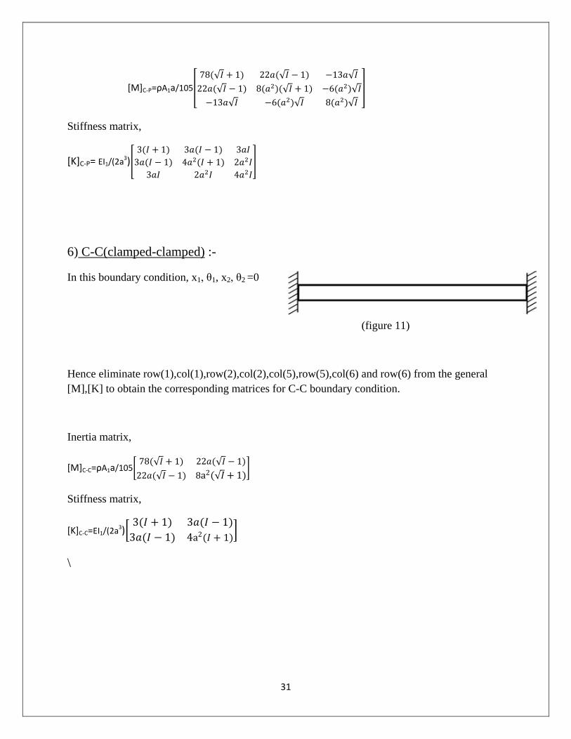
6) C-C(clamped-clamped) :-

In this boundary condition, x1, θ1, x2, θ2 =0

(figure 11)

Hence eliminate row(1),col(1),row(2),col(2),col(5),row(5),col(6) and row(6) from the general [M],[K] to obtain the corresponding matrices for C-C boundary condition.

Inertia matrix,

[M]C-C=ρA1a/105�78(√𝐼 + 1) 22𝑎(√𝐼 − 1)

22𝑎(√𝐼 − 1) 8a2(√𝐼+ 1)�

Stiffness matrix,

[K]C-C=EI1/(2a3)�3(𝐼 + 1) 3𝑎(𝐼 − 1)

3𝑎(𝐼 − 1) 4a2(𝐼 + 1)�

\

31

7)C-S(clamped-slide) :-

In this boundary condition, x1, θ1, θ2 =0

(figure 12)

Hence eliminate row(1),col(1),row(2),col(2),col(6) and row(6) from the general [M],[K] to obtain the corresponding matrices for C-S boundary condition.

Inertia matrix,

[M]C-S=ρA1a/105�78(√𝐼 + 1) 22𝑎(√𝐼 − 1) 27√𝐼

22𝑎(√𝐼 − 1) 8(𝑎2)(√𝐼 + 1) 13𝑎√𝐼27√𝐼 13𝑎√𝐼 78√𝐼

�

Stiffness matrix,

[K]C-S= EI1/(2a3)�3(𝐼 + 1) 3𝑎(𝐼 − 1) −3𝐼

3𝑎(𝐼 − 1) 4𝑎2(𝐼 + 1) −3𝑎𝐼−3𝐼 −3𝑎𝐼 3𝐼

�

8)S-P(slide-pinned) :-

In this boundary condition, θ2, x2 =0

(figure 13)

Hence eliminate row(2),col(2),col(5) and row(5) from the general [M],[K] to obtain the corresponding matrices for S-P boundary condition.

32

Inertia matrix,

[M]S-P=ρA1a/105

−−

−+−−

−−+

−

IaIaIa

IaIaIaa

IaIaI

a

2^82^6130

2^6)1(2^8)1(2213

13)1(22)1(7827

0132778

Stiffness matrix,

[K]S-P= EI1/ (2a3)

+−−+−

−

IaIaaIIaIaIa

aIIaIa

)2^(4)2^(230)2^(2)1)(2^(4)1(33

3)1(3)1(330333

9)S-S(sliding-sliding) :-

In this case, θ1,θ2=0

Hence eliminate row(2),col(2),col(6) and row(6) from the general [M],[K] to obtain the corresponding matrices for S-S condition.

Inertia matrix, . . . . . . . (figure 14)

[M]S-S=ρA1a/105

+−−

−+

−

IIaI

IaIaIaa

IIaI

a

7813270

13)1(2^8)1(2213

27)1(22)1(7827

0132778

Stiffness matrix,

[K]S-S= EI1/(2a3)

−−−+−−−+−

−

IaIIaIIaIaIIaI

a

33303)1)(2^(4)1(333)1(3)1(330333

33

Chapter – 4

RESULTS

34

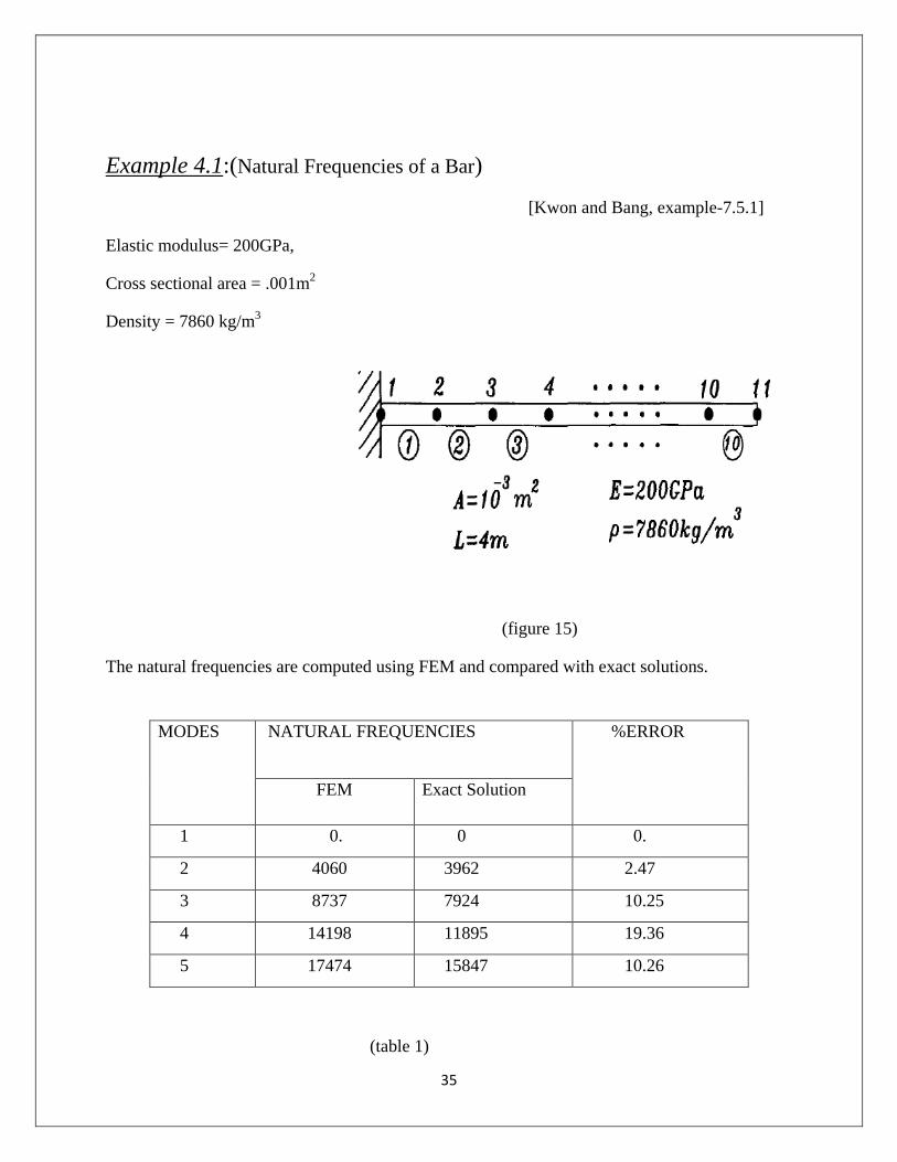
Example 4.1:(Natural Frequencies of a Bar)

[Kwon and Bang, example-7.5.1]

Elastic modulus= 200GPa,

Cross sectional area = .001m2

Density = 7860 kg/m3

(figure 15)

The natural frequencies are computed using FEM and compared with exact solutions.

(table 1)

MODES NATURAL FREQUENCIES %ERROR

FEM Exact Solution

1 0. 0 0.

2 4060 3962 2.47

3 8737 7924 10.25

4 14198 11895 19.36

5 17474 15847 10.26

35

EXAMPLE 4.2 : (natural frequency of a truss)

[Kwon and Bang,7.5.2]

Each member of the truss shown has the density of 7860 kg/m3

(figure 16)

The first five natural frequencies of the above truss structure were given below.

1st natural frequency = 240.9 rad/s

2nd natural frequency = 467.9 rad/s

3rd natural frequency = 739.8rad/s

4th natural frequency = 1243rad/s

5th natural frequency = 1633rad/s

36

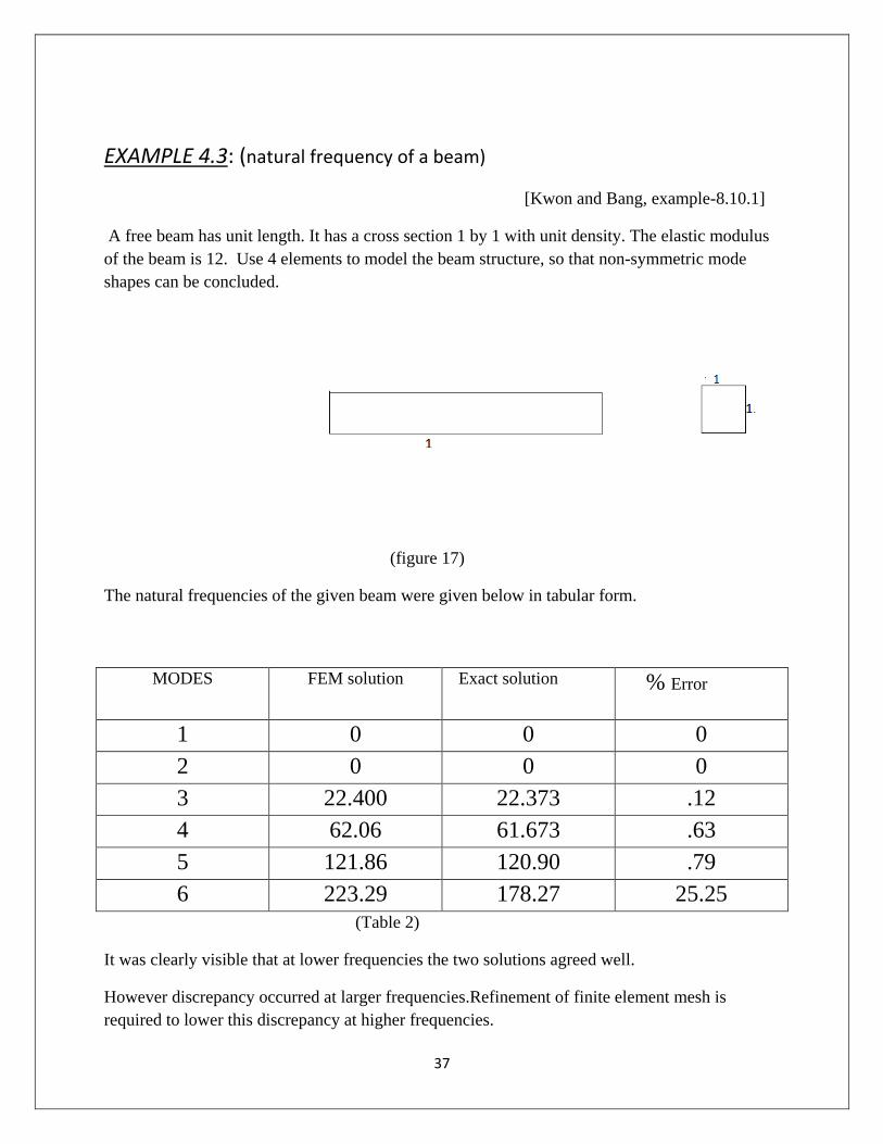
EXAMPLE 4.3: (natural frequency of a beam)

[Kwon and Bang, example-8.10.1]

A free beam has unit length. It has a cross section 1 by 1 with unit density. The elastic modulus of the beam is 12. Use 4 elements to model the beam structure, so that non-symmetric mode shapes can be concluded.

(figure 17)

The natural frequencies of the given beam were given below in tabular form.

MODES FEM solution Exact solution % Error

1 0 0 0 2 0 0 0 3 22.400 22.373 .12 4 62.06 61.673 .63 5 121.86 120.90 .79 6 223.29 178.27 25.25

(Table 2)

It was clearly visible that at lower frequencies the two solutions agreed well.

However discrepancy occurred at larger frequencies.Refinement of finite element mesh is required to lower this discrepancy at higher frequencies.

37

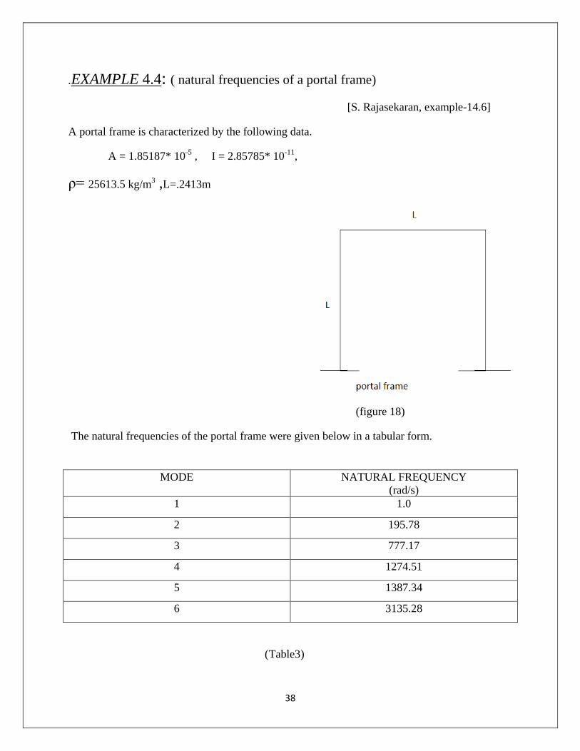
.EXAMPLE 4.4: ( natural frequencies of a portal frame)

[S. Rajasekaran, example-14.6]

A portal frame is characterized by the following data.

A = 1.85187* 10-5 , I = 2.85785* 10-11,

ρ= 25613.5 kg/m3 ,L=.2413m

(figure 18)

The natural frequencies of the portal frame were given below in a tabular form.

(.Table3.)

MODE NATURAL FREQUENCY (rad/s)

1 1.0

2 195.78

3 777.17

4 1274.51

5 1387.34

6 3135.28

38

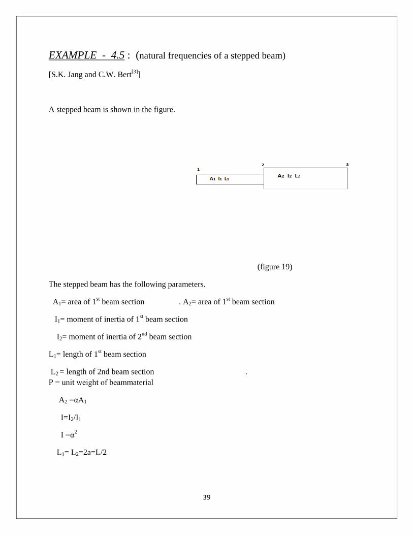
EXAMPLE - 4.5 : (natural frequencies of a stepped beam)

[S.K. Jang and C.W. Bert[3]]

A stepped beam is shown in the figure.

(figure 19)

The stepped beam has the following parameters.

A1= area of 1st beam section . A2= area of 1st beam section

I1= moment of inertia of 1st beam section

I2= moment of inertia of 2nd beam section

L1= length of 1st beam section

L2 = length of 2nd beam section . Ρ = unit weight of beammaterial

A2 =αA1

I=I2/I1

I =α2

L1= L2=2a=L/2

39

TABLE :-

Natural frequencies,ω’= ω/L2(EI1/ρA1)1/2 of fundamental modefor various boundary conditions were given below in a tabular form.

Boundary Conditions

I (=I2/I1)

Exact Solution

FEM Result

% error

Pinned-pinned (P-P)

1 9.8696 9.9086 .395 5 10.4129 10.4441 .299 10 9.8781 9.9002 .223 20 9.0747 9.0885 .152 40 8.1369 8.1448 .097

Clamped –clamped (C-C)

1 22.3733 22.7375 1.620 5 25.9591 26.3573 1.534 10 27.6807 28.0922 1.486 20 30.3213 30.7716 1.485 40 34.3252 34.8702 1.587

Clamped- Free (C-F)

1 3.5160 3.5177 .048 5 2.4373 2.4376 .012 10 2.0629 2.0630 .004 20 1.7418 1.7418 0 40 1.4685 1.4685 0

Clamped- Pinned (C-P)

1 15.4182 15.5608 .924 5 16.2811 16.3761 .583 10 15.5129 15.5783 .421 20 14.2568 14.2967 .279 40 12.7501 12.7721 .172

Free - Free (F-F)

1 22.3733 22.4234 .223 5 24.1650 24.2127 .197 10 23.5459 23.5809 .137 20 22.4725 22.5056 .147 40 21.1907 21.2306 .188

Slide - Slide (S-S)

1 9.8696 9.9101 .410 5 13.5124 13.5919 .588 10 15.9066 16.0330 .794 20 18.2949 18.4909 1.070 40 20.1954 20.4501 1.261

40

Boundary Condition

I Exact solution FEM solution %error

Slide – Pinned (S-P)

1 2.4674 2.4680 .024

5 2.4372 2.4377 .020

10 2.3292 2.3296 .017

20 2.1814 2.1844 .013

40 2.0122 2.0124 .009

Clamped – Slide (C-S)

1 5.5933 5.6007 .132

5 5.6912 5.6950 .066

10 5.6321 5.6340 .033

20 5.3573 5.3590 .031

40 4.8913 4.8922 .018

Free – Slide (F-S)

1 5.5933 5.5994 .109

5 9.3624 9.3807 .195

10 11.0519 11.0924 .336

20 12.4070 12.4513 .357

40 13.2947 13.3481 .401

Free- Pinned (F-P)

1 15.4182 15.5142 .622

5 18.6102 18.6838 .395

10 18.7641 18.8202 .298

20 18.4031 18.4566 .290

40 17.7778 17.8301 .294

(.table 4.)

41

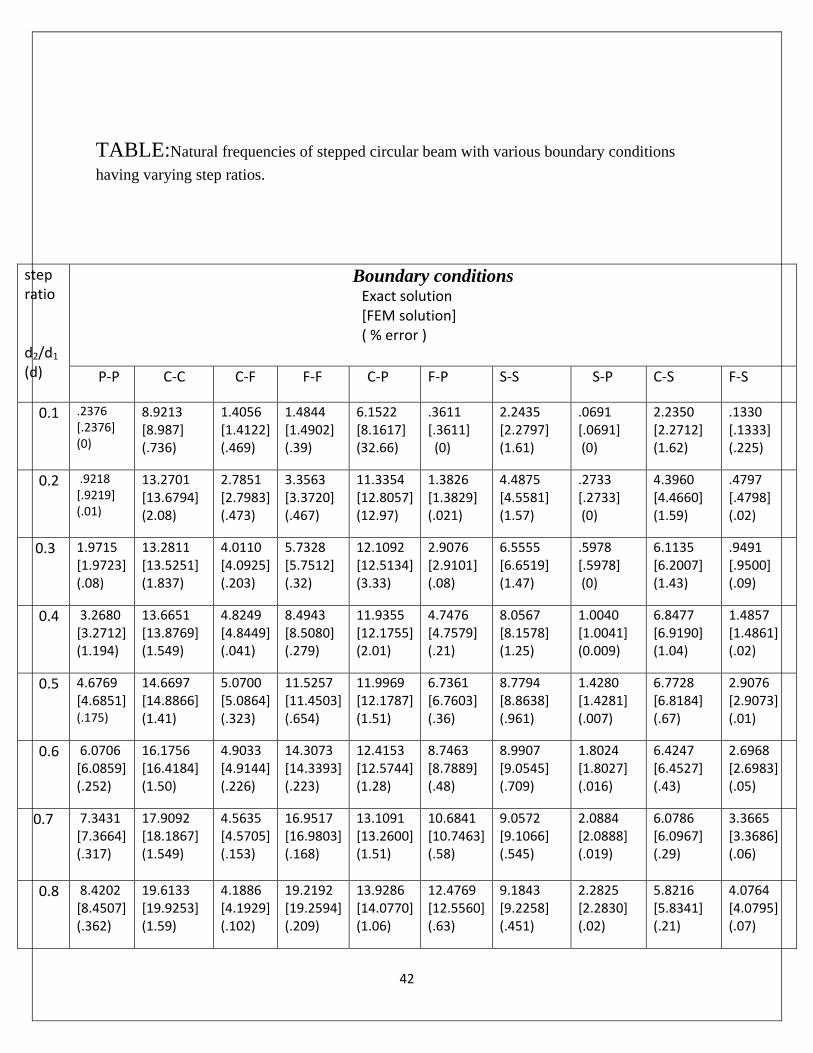
TABLE:Natural frequencies of stepped circular beam with various boundary conditions having varying step ratios.

step ratio d2/d1

(d)

Boundary conditions Exact solution [FEM solution] ( % error )

P-P C-C C-F F-F C-P F-P S-S S-P C-S F-S

0.1 .2376 [.2376] (0)

8.9213 [8.987] (.736)

1.4056 [1.4122] (.469)

1.4844 [1.4902] (.39)

6.1522 [8.1617] (32.66)

.3611 [.3611] (0)

2.2435 [2.2797] (1.61)

.0691 [.0691] (0)

2.2350 [2.2712] (1.62)

.1330 [.1333] (.225)

0.2 .9218 [.9219] (.01)

13.2701 [13.6794] (2.08)

2.7851 [2.7983] (.473)

3.3563 [3.3720] (.467)

11.3354 [12.8057] (12.97)

1.3826 [1.3829] (.021)

4.4875 [4.5581] (1.57)

.2733 [.2733] (0)

4.3960 [4.4660] (1.59)

.4797 [.4798] (.02)

0.3 1.9715 [1.9723] (.08)

13.2811 [13.5251] (1.837)

4.0110 [4.0925] (.203)

5.7328 [5.7512] (.32)

12.1092 [12.5134] (3.33)

2.9076 [2.9101] (.08)

6.5555 [6.6519] (1.47)

.5978 [.5978] (0)

6.1135 [6.2007] (1.43)

.9491 [.9500] (.09)

0.4 3.2680 [3.2712] (1.194)

13.6651 [13.8769] (1.549)

4.8249 [4.8449] (.041)

8.4943 [8.5080] (.279)

11.9355 [12.1755] (2.01)

4.7476 [4.7579] (.21)

8.0567 [8.1578] (1.25)

1.0040 [1.0041] (0.009)

6.8477 [6.9190] (1.04)

1.4857 [1.4861] (.02)

0.5 4.6769 [4.6851] (.175)

14.6697 [14.8866] (1.41)

5.0700 [5.0864] (.323)

11.5257 [11.4503] (.654)

11.9969 [12.1787] (1.51)

6.7361 [6.7603] (.36)

8.7794 [8.8638] (.961)

1.4280 [1.4281] (.007)

6.7728 [6.8184] (.67)

2.9076 [2.9073] (.01)

0.6 6.0706 [6.0859] (.252)

16.1756 [16.4184] (1.50)

4.9033 [4.9144] (.226)

14.3073 [14.3393] (.223)

12.4153 [12.5744] (1.28)

8.7463 [8.7889] (.48)

8.9907 [9.0545] (.709)

1.8024 [1.8027] (.016)

6.4247 [6.4527] (.43)

2.6968 [2.6983] (.05)

0.7 7.3431 [7.3664] (.317)

17.9092 [18.1867] (1.549)

4.5635 [4.5705] (.153)

16.9517 [16.9803] (.168)

13.1091 [13.2600] (1.51)

10.6841 [10.7463] (.58)

9.0572 [9.1066] (.545)

2.0884 [2.0888] (.019)

6.0786 [6.0967] (.29)

3.3665 [3.3686] (.06)

0.8 8.4202 [8.4507] (.362)

19.6133 [19.9253] (1.59)

4.1886 [4.1929] (.102)

19.2192 [19.2594] (.209)

13.9286 [14.0770] (1.06)

12.4769 [12.5560] (.63)

9.1843 [9.2258] (.451)

2.2825 [2.2830] (.02)

5.8216 [5.8341] (.21)

4.0764 [4.0795] (.07)

42

(Table 5.)

0.9 9.2635 [9.2994] (.387)

21.1232 [21.4641] (1.613)

3.8338 [3.8365] (.07)

21.0307 [21.0770] (.22)

14.7321 [14.8786] (.99)

14.0680 [14.1587] (.64)

9.4500 [9.4885] (.407)

2.4018 [2.4025] (.03)

5.6652 [5.6746] (.16)

4.8215 [4.8259] (.09)

1.0 9.8696 [9.9086] (.395)

22.3733 [22.7359] (1.62)

3.5160 [3.5177] (.048)

22.3733 [22.4210] (.213)

15.4182 [15.5608] (.92)

15.4182 [15.5142] (.62)

9.8696 [9.9101] (.41)

2.4674 [2.4680] (.02)

5.5933 [5.6007] (.13)

5.5933 [5.5994] (.109)

2 9.3538 [9.3701] (.174)

29.3393 [29.7732] (1.478)

1.8397 [1.8397] (0)

22.8515 [22.8852] (.147)

14.6995 [14.7468] (.32)

18.5595 [18.6100] (.27)

17.5587 [17.7275] (.961)

2.2342 [2.2346] (.018)

5.4699 [5.4719] (.04)

12.0199 [12.0611] (.34)

3 7.1485 [7.1526] (.057)

40.0354 [40.7176] (1.70)

1.2332 [1.2332] (0)

19.8611 [19.9003] (.019)

11.1549 [11.1660] (.09)

17.0666 [17.1201] (.31)

21.4171 [21.7198] (1.41)

1.8200 [1.8201] (.005)

4.3144 [4.3149] (.01)

13.7883 [13.8471] (.42)

4 5.6310 [5.6322] (.021)

53.0768 [54.2360] (2.18)

.9264 [.9261] (.034)

17.9407 [18.0013] (.337)

8.7256 [8.7287] (.03)

16.0259 [16.0800] (.34)

22.2601 [22.6001] (1.527)

1.4958 [1.4959] (.006)

3.3700 [3.3701] (.002)

14.0871 [14.1504] (.45)

5 4.6089 [4.6097] (.017)

66.3507 [68.3972] (3.08)

.7417 [.7420] (.04)

16.7816 [16.8102] (.17)

7.1104 [7.1100] (.005)

15.4132 [15.5120] (.64)

22.4377 [22.7906] (1.572)

1.2559 [1.3000] (3.51)

2.7325 [2.7326] (.003)

14.1349 [14.2012] (.47)

6 3.8887 [3.9013] (.324)

78.4064 [82.7020] (5.47)

.6183 [.6183] (0)

16.0549 [16.1232] (.425)

5.9831 [6.0016] (.309)

15.0391 [15.1003] (.41)

22.4702 [22.8276] (1.59)

1.0765 [1.1000] (2.18)

2.2901 [2.2901] (0)

14.1348 [14.2031] (.48)

7 3.3582 [3.3496] (.256)

85.8217 [97.0236] (13.05)

.5301 [.5345] (.83)

15.5772 [15.6213] (.283)

5.1577 [5.2000] (.82)

14.7981 [14.9078] (.74)

22.4676 [22.8276] (1.60)

.9392 [.9301] (.97)

1.9685 [2.0001] (1.6)

14.1256 [14.2009] (.53)

8 2.9528 [3.0012] (1.639)

88.1235 [98.1254] (15.64)

.4639 [.5003] (7.7)

15.2493 [15.3098] (.396)

4.5296 [4.5001] (.65)

14.6352 [14.7103] (.51)

22.4569 [22.8157] (1.583)

.8316 [.8012] (3.65)

1.7252 [1.7101] (.87)

14.1159 [14.2001] (.59)

9 2.6335 [2.6351] (.060)

88.8330 [99.2354] (16.01)

.4124 [.4456] (8.05)

15.0156 [15.1908] (.987)

4.0363 [4.0011] (.87)

14.5203 [14.6011] (.55)

22.4456 [22.8434] (1.77)

.7453 [.7230] (2.9)

1.5351 [1.5129] (1.45)

14.1076 [14.2023] (.67)

10

2.3758 [2.4001] (1.02)

89.1225 [103.3244] (19.87)

.3718 [.4120] (10.81)

14.8439 [14.9103] (.447)

3.6391 [3.6000] (1.07)

14.4366 [14.5130] (.53)

22.4354 [22.8396] (1.80)

.6748 [.7010] (3.9)

1.3825 [1.4012] (.97)

14.1008 [14.2034] (.73)

43

GRAPH:

Graph of natural frequencies vs step ratio for various boundary conditions, was plotted below.

(Figure 20)

44

Chapter – 5

CONCLUSION AND

DISCUSSION

45

CONCLUSION :

FEM results showed quite fair accuracy when compared with the analytical methods.

%error in FEM can be minimized by increasing the finite elements and refinement of finite mesh which is not so difficult to compute by the help of computer.

FEM was quite efficient and better than the analytical in case of any irregularity or complexity of the structures.

FEM calculations in addition with MATLAB codes form a powerful medium for vibration analysis of irregular structures with many advantages over all other methods out there.

46

DISCUSSION:

FEM is effective in analyzing the physical properties, which are complex for any closed bound

solution.

FEM is quite effective and time saving tool for solving the vibration analysis of any kind of

structures from linear to complex non-linear structures.

It is simple to use unlike the tedious analytical methods. It is meant for modern world problems

and it can be easily programmed with computers and, various structural softwares heavily

depend upon FEM.

When a continuum is discretized, an infinite degrees of freedom system is converted into a

model having finite number of degrees of freedom. The accuracy depends to a great extent on the

mesh grading of the continuum.

In regions of high strain gradient, higher gradation of finite element mesh is needed whereas in

the regions of lower strain, the mesh chosen may be coarser. As the element size decreases, the

discretization error reduces.

47

REFERENCES

48

1. Young W. Kwon and Bang H., “Finite Element Method using MATLAB,” CRC press(1997)

2. Asghar Bhatti M., “Fundamental Finite Element Analysis and Applications”

John Wiley & Sons Inc. 2005

3. Jang S.K.and Bert C.W., “Free Vibration of Stepped Beams,” Journal of Sound and Vibration130,(1989) 342-346

4. Blevins R.D., “ Formulas for Natural Frequency and Mode Shape,” (1979) New York -Van Nostrand, 108-109

5. Balasubramanian T.S. and Subramanian G., “On performance of a four-degree of freedom per node element for stepped beam analysis and higher frequency estimation,” Journal of Sound and Vibration 99(1985),563-567

6. Subramanian G. and Balasubramanian T.S., “Beneficial effects of steps on the free vibration characteristics of beams,” Journal of Sound and Vibration118(1987), 555-560

7. GORMAN D. J.1975 Free Vibration Analysis of Beams and Shafts. New York: John Wiley and Sons.

8. Klein Larisse, “Transverse Vibration of non-uniform Beams,” Journal of Sound and Vibration37(1974) I(4) 491-505

9. Gladwell G.M.L., “ The Vibration of Frames,” Journal of Sound and Vibration1(1964) I(4) 402-425

10. RajasekaranS., “Structural Dynamics of Earthquake Engineering : theory and

application using MATHEMATICA and MATLAB,” woodhead publishing limited (2009)

11. Petyt Maurice, “Introduction to Finite Element Vibration Analysis,” Cambridge

University Press(1990)

49