free energy calculations in biological systems. how useful are

Free Energy Calculations in Biological Systems.How Useful Are They in Practice?

Christophe Chipot

Equipe de dynamique des assemblages membranaires, UMR CNRS/UHP 7565,Institut nancéien de chimie moléculaire, Université Henri Poincaré, BP 239,54506 Vandœuvre–lès–Nancy cedex, France

Abstract. Applications of molecular simulations targeted at the estimation of free energiesare reviewed, with a glimpse into their promising future. The methodological milestonespaving the road of free energy calculations are summarized, in particular free energy per-turbation and thermodynamic integration, in the framework of constrained or unconstrainedmolecular dynamics. The continuing difficulties encountered when attempting to obtain ac-curate estimates are discussed with an emphasis on the usefulness of large–scale numericalsimulations in non–academic environments, like the world of the pharmaceutical industry.Applications of the free energy arsenal of methods is illustrated through a variety of biologi-cally relevant problems, among which the prediction of protein–ligand binding constants, thedetermination of membrane–water partition coefficients of small, pharmacologically activecompounds — in connection with the blood–brain barrier, the folding of a short hydropho-bic peptide, and the association of transmembrane α–helical domains, in line with the “two–stage” model of membrane protein folding. Current strategies for improving the reliability offree energy calculations, while making them somewhat more affordable, and, therefore, morecompatible with the constraints of an industrial environment, are outlined.

Key words: Free energy calculations, molecular dynamics simulations, drug design,protein folding, protein recognition and association

1 Introduction

To understand fully the vast majority of chemical and biochemical processes, a closeexamination of the underlying free energy behavior is often necessary [1]. Such isthe case, for instance, of protein–ligand binding constants and membrane–water par-tition coefficients, that are of paramount important in the emerging field of de novo,rational drug design, and cannot be predicted reliably and accurately without theknowledge of the associated free energy changes. The ability to determine a priorithese physical constants with a reasonable level of accuracy, by means of statisticalsimulations, is now within reach. Developments on both the software and the hard-ware fronts have contributed to bring free energy calculations at the level of similarly

184 C. Chipot

robust and well–characterized modeling tools, while widening their field of applica-tions. Yet, in spite of the tremendous progress accomplished since the first publishedcalculations some twenty years ago [2–5], the accurate estimation of free energychanges in large, physically and biologically realistic molecular assemblies still con-stitutes a challenge for modern theoretical chemistry. Taking advantage of massivelyparallel architectures, cost–effective, “state–of–the–art” free energy calculations canprovide a convincing answer to help rationalizing experimental observations, and, insome instances, play a predictive role in the development of new leads for a specifictarget.

In the first section of this chapter, the methodological background of free en-ergy calculations is developed, focusing on the methods that are currently utilizedto determine free energy differences. Next, four biologically relevant applicationsare presented, corresponding to distinct facets of free energy simulations. The firstone delves into the use of these calculations in de novo drug design, through theestimation of protein–ligand binding affinities and water–membrane partition coef-ficients. The somewhat more challenging application of molecular dynamics (MD)simulations and free energy methods to validate the three–dimensional structure ofa G protein–coupled receptor (GPCR) is shown next. Understanding of the intricatephysical phenomena that drive protein folding by means of free energy calculationsis also reported here, followed by an investigation of the reversible association oftransmembrane (TM) α–helices in a membrane mimetic. Conclusions on the roleplayed by free energy calculations in the molecular modeling community are drawnwith a prospective look into their future.

2 Methodological Background

In the canonical, (N,V, T ), ensemble, the Helmholtz free energy is defined by [6]:

A = − 1β

lnQNVT (1)

β = 1/kBT , where kB is the Boltzmann constant and T is the temperature of theN–particle system. QNVT is its 6N–dimensional partition function:

QNVT =1

h3NN !

∫ ∫exp [−βH(x,px)] dx dpx (2)

where H(x,px) is the classical Hamiltonian describing the system. In (2), integra-tion is carried out over all atomic coordinates, {x}, and momenta, {px}. The nor-malization factor reflects the measure of the volume of the phase space through thePlanck constant, h, and the indistinguishable nature of the particles, embodied in thefactorial term, N !. In essence, the canonical partition function constitutes the cornerstone of the statistical mechanical description of the ensemble of particles. From aphenomenological perspective, it may be viewed as a measure of the thermodynamicstates accessible to the system in terms of spatial coordinates and momenta. It can befurther restated in terms of energies:

Free Energy Calculations 185

QNVT =1

h3NN !

∫�[H(x,px)] exp [−βH(x,px)] dH(x,px) (3)

where �[H(x,px)] is the so–called density of states accessible to the system of in-terest.

The definition of the partition function may be utilized to introduce the conceptof probability distribution to find the system in the unique microscopic state charac-terized by positions {x} and momenta {px}:

P(x,px) =1

h3NN !1

QNVTexp [−βH(x,px)] (4)

A logical consequence of this expression is that low–energy regions of thephase space will be sampled predominantly, according to their respective Boltzmannweight [7].

2.1 Free Energy Perturbation

Returning to the original definition (1) of the free energy, and using the identity:∫ ∫exp [+βH(x,px)] exp [−βH(x,px)] dx dpx = h3NN ! (5)

it follows that:

A = − 1β

ln1

h3NN !

∫ ∫exp [−βH(x,px)] dx dpx

= +1β

ln∫ ∫

exp [+βH(x,px)] P(x,px) dx dpx

= +1β

ln 〈exp [+βH(x,px)]〉 (6)

This expression illuminates the fast growth of exp [+βH(x,px)] with the totalenergy, H(x,px), of the system. It should, therefore, be expected that the weightof the high–energy regions of phase space be significant when evaluating the inte-gral. Yet, as hinted by (4), in simulations of finite length, sampling of these regionsis likely to be insufficient to guarantee a correct estimate of A. In most instances,evaluation of accurate absolute free energies from statistical simulations is not pos-sible. The latter may, however, give access to free energy differences between twowell–delineated thermodynamic states, provided that a reaction coordinate can bedefined to characterize the pathway that connects these two states. In this context,the Hamiltonian, H(x,px), describing the transformation is made a function of thereaction coordinate, or “coupling parameter”, λ [8]. Conventionally, λ varies be-tween 0 and 1 when the system goes from the initial state, a, to the final state, b,

186 C. Chipot

characterized, respectively, by the Hamiltonians H(x,px;λa) = H(x,px;λ = 0)and H(x,px;λb) = H(x,px;λ = 1) . In practice, λ can correspond to a varietyof reaction coordinates, ranging from a simple distance to determine a potential ofmean force (PMF) to non–bonded parameters in the so–called “alchemical transfor-mations” or in silico point mutations [4, 5].

Within this framework, the canonical partition function defined in (2) now de-pends explicitly on the coupling parameter, and so does the free energy:

∆Aa→b = A(λb) −A(λa) = − 1β

lnQNVT(λb)QNVT(λa)

(7)

Combining the above with the definition of the partition function, and introducingthe identity (5), it follows that:

∆Aa→b = − 1β

ln 〈exp {−β [H(x,px;λb) −H(x,px;λa)]}〉λa(8)

Here, 〈· · · 〉λadenotes an ensemble average over configurations representative of the

initial state, a. Validity of perturbation formula (8) only holds for small changesbetween the initial state, a, and the final state, b, of the transformation [9]. At thisstage, the condition of small changes should be clarified, as it has often been mis-construed in the past. It does not imply that the free energies characteristic of a andb be sufficiently close, but rather that the corresponding configurational ensemblesoverlap appropriately to guarantee the desired accuracy [10, 11]. In other words, it isexpected that the density of states, �[H(x,px)], describing the transformation froma to b be narrow enough — viz. typically on the order of 1 / β, to ascertain that,when multiplied by the exponential term of (3), the resulting distribution be locatedin a region where ample statistical data have been collected. In most circumstances,however, single–step transformations between rather orthogonal states are unlikely tofulfill this requirement. To circumvent this difficulty, the reaction pathway is brokendown into a number of physically meaningless intermediate states connecting a to b,so that between any two contiguous states, the condition of overlapping ensembles issatisfied [12]. The interval separating these intermediate states, which corresponds toselected fixed values of the coupling parameter, λ, is often referred to as “window”.It should be reminded that the vocabulary window adopted in perturbation theory isdistinct from that utilized in “umbrella sampling” (US) simulations [13], where itdenotes a range of values taken by the reaction coordinate. For a series of a N in-termediate states, the total free energy change for the transformation from a to b isexpressed as a sum of N − 1 free energy differences [12]:

∆Aa→b = − 1β

N−1∑k=1

ln 〈exp {−β [H(x,px;λk+1) −H(x,px;λk)]}〉λk(9)

Assessing the ideal number of intermediate states, N , between a and b evidently de-pends upon the nature of the system that undergoes the transformation. The conditionof overlapping ensembles should be kept in mind when setting N , remembering that


the choice of δλ = λk+1 − λk ought to correspond to a perturbation of the system.A natural choice consists in using a number of windows that guarantees a reasonablysimilar free energy change between contiguous intermediate states. The consequenceof this choice is that the width of the consecutive windows connecting a to b may bedifferent.

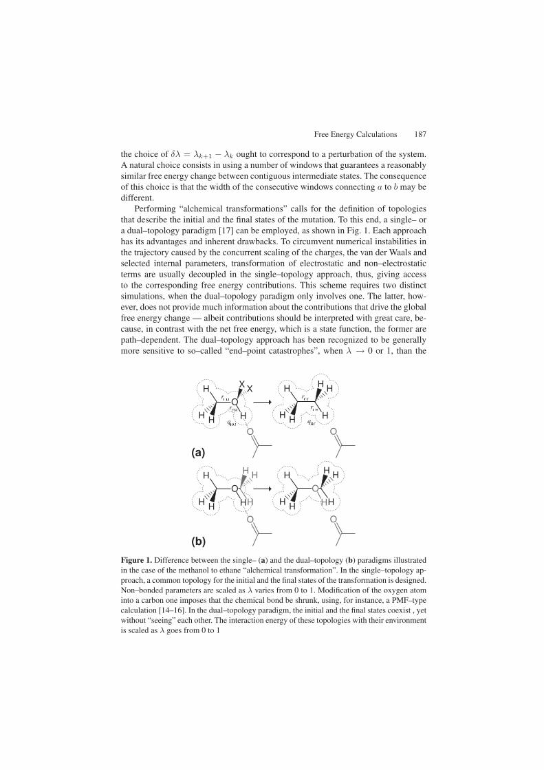
Performing “alchemical transformations” calls for the definition of topologiesthat describe the initial and the final states of the mutation. To this end, a single– ora dual–topology paradigm [17] can be employed, as shown in Fig. 1. Each approachhas its advantages and inherent drawbacks. To circumvent numerical instabilities inthe trajectory caused by the concurrent scaling of the charges, the van der Waals andselected internal parameters, transformation of electrostatic and non–electrostaticterms are usually decoupled in the single–topology approach, thus, giving accessto the corresponding free energy contributions. This scheme requires two distinctsimulations, when the dual–topology paradigm only involves one. The latter, how-ever, does not provide much information about the contributions that drive the globalfree energy change — albeit contributions should be interpreted with great care, be-cause, in contrast with the net free energy, which is a state function, the former arepath–dependent. The dual–topology approach has been recognized to be generallymore sensitive to so–called “end–point catastrophes”, when λ → 0 or 1, than the

Figure 1. Difference between the single– (a) and the dual–topology (b) paradigms illustratedin the case of the methanol to ethane “alchemical transformation”. In the single–topology ap-proach, a common topology for the initial and the final states of the transformation is designed.Non–bonded parameters are scaled as λ varies from 0 to 1. Modification of the oxygen atominto a carbon one imposes that the chemical bond be shrunk, using, for instance, a PMF–typecalculation [14–16]. In the dual–topology paradigm, the initial and the final states coexist , yetwithout “seeing” each other. The interaction energy of these topologies with their environmentis scaled as λ goes from 0 to 1

188 C. Chipot

single–topology paradigm. A number of schemes have been devised to circumventthis problem, among which the use of windows of decreasing width as λ tends to-wards 0 or 1. Introduction of a soft–core potential [18] to eliminate the singularitiesat 0 or 1 perhaps constitutes the most elegant method proposed hitherto.

2.2 Thermodynamic Integration

Closely related to the free energy perturbation (FEP) expression, thermodynamicintegration (TI) restates the free energy difference between state a and state b as afinite difference [8, 19]:

∆Aa→b = A(λb) −A(λa) =∫ λb

λa

dA(λ)dλ

dλ (10)

Combining with the definition of the canonical partition function (2), it follows that:

dA(λ)dλ

=

∫∂H(x,px;λ)

∂λexp−βH(x,px;λ) dx dpx∫

exp−βH(x,px;λ) dx dpx

(11)

Consequently, the integrand can be written as an ensemble average:

∆Aa→b =∫ λb

λa

⟨∂H(x,px;λ)

∂λ

⟩λ

dλ (12)

In sharp contrast with the FEP method, the criterion of convergence here is theappropriate smoothness of A(λ). Interestingly enough, assuming that the variation ofthe kinetic energy between states a and b can be neglected, the derivative of ∆Aa→b

with respect to some reaction coordinate, ξ , is equal to, −〈Fξ〉ξ , the average of theforce exerted along ξ , hence, the concept of PMF [20].

2.3 Unconstrained Molecular Dynamics and Average Forces

Generalization of the classical definition of a PMF, w(r), based on the pair corre-lation function, g(r), is not straightforward. For this reason, the free energy as afunction of reaction coordinate ξ will be expressed as:

A(ξ) = − 1β

lnP(ξ) + A0 (13)

where P(ξ) is the probability distribution to find the system at a given value, ξ, alongthat reaction coordinate:

P(ξ) =∫

δ[ξ − ξ(x)] exp[−βH(x,px)] dx dpx (14)


Equation (13) corresponds to the classic definition of the free energy in methodslike US, in which external biasing potentials are included to ensure a uniform dis-tribution P(ξ). To improve sampling efficiency, the complete reaction pathway isbroken down into “windows”, or ranges of ξ, wherein individual free energy profilesare determined. The latter are subsequently pasted together using, for instance, theself–consistent weighted histogram analysis method (WHAM) [21].

For a number of years, the first derivative of the free energy with respect to thereaction coordinate has been written as [22]:

dA(ξ)dξ

=⟨∂V(x)∂ξ

⟩ξ

(15)

This description is erroneous because ξ and {x} are evidently not independent vari-ables [23]. Furthermore, it assumes that kinetic contributions can be safely omitted.This may not always be necessarily the case. For these reasons, a transformation ofthe metric is required, so that:

P(ξ) =∫

|J | exp[−βV(q; ξ)] dq∫

exp[−βT (px)]dpx (16)

Introduction in the first derivative of probability P(ξ), it follows that the kineticcontribution vanishes in dA(ξ)/dξ:

dA(ξ)dξ

= − 1β

1P(ξ)

∫exp[−βV(q; ξ∗)] δ(ξ∗ − ξ) ×

{−β|J |∂V(q; ξ∗)

∂ξ+

∂|J |∂ξ

}dq dξ∗ (17)

After back transformation into Cartesian coordinates, the derivative of the free en-ergy with respect to ξ can be expressed as a sum of configurational averages at con-stant ξ [24]:

dA(ξ)dξ

=⟨∂V(x)∂ξ

⟩ξ

− 1β

⟨∂ ln |J |

∂ξ

⟩ξ

= −〈Fξ〉ξ (18)

In this approach, only 〈Fξ〉ξ is the physically meaningful quantity, unlike the instan-taneous components, Fξ, from which it is evaluated. Moreover, it should be clearlyunderstood that neither Fξ nor −∂H(x,px)/∂ξ are fully defined by the sole choiceof the reaction coordinate.

In practice, Fξ is accumulated in bins of finite size δξ and provides an estimateof dA(ξ)/dξ. After a predefined number of observables are accrued, the adaptivebiasing force (ABF) [25, 26] is applied along the reaction coordinate:

FABF = ∇A = −〈Fξ〉ξ ∇ξ (19)

190 C. Chipot

As sampling proceeds, ∇A is progressively refined. Evolution of the system alongξ is governed mainly by its self–diffusion properties. It is apparent from the presentdescription that this method is significantly more effective than US or its variants,because no a priori knowledge of the free energy hypersurface is required to definethe necessary biasing potentials that will guarantee uniform sampling along ξ. Thelatter can easily become intricate in the case of qualitatively new problems, in whichvariation of the free energy behavior cannot be guessed with the appropriate accu-racy. Often misconstrued, it should be emphasized that, whereas ABF undoubtedlyimproves sampling dramatically along the reaction coordinate, efficiency suffers, likeany other free energy method, from orthogonal degrees of freedom in the slow man-ifolds.

2.4 When is Enough Sampling Really Enough?

When is the trajectory long enough to assume safely that the results are converged? isa recurrent question asked by modelers performing free energy calculations. Assess-ing the convergence properties and the error associated to a free energy calculationoften turns out to be daunting task. Sources of errors likely to be at play are diverse,and, hence, will modulate the results differently. The choice of the force field para-meters undoubtedly affects the results of the simulation, but this contribution can belargely concealed by the statistical error arising from insufficient sampling. Paradox-ically, exceedingly short free energy calculations employing inadequate non–bondedparameters may, nonetheless, yield the correct answer [14]. Under the hypotheticalassumption of an optimally designed potential energy function, quasi non–ergodicityscenarios constitute a common pitfall towards fully converged simulations.

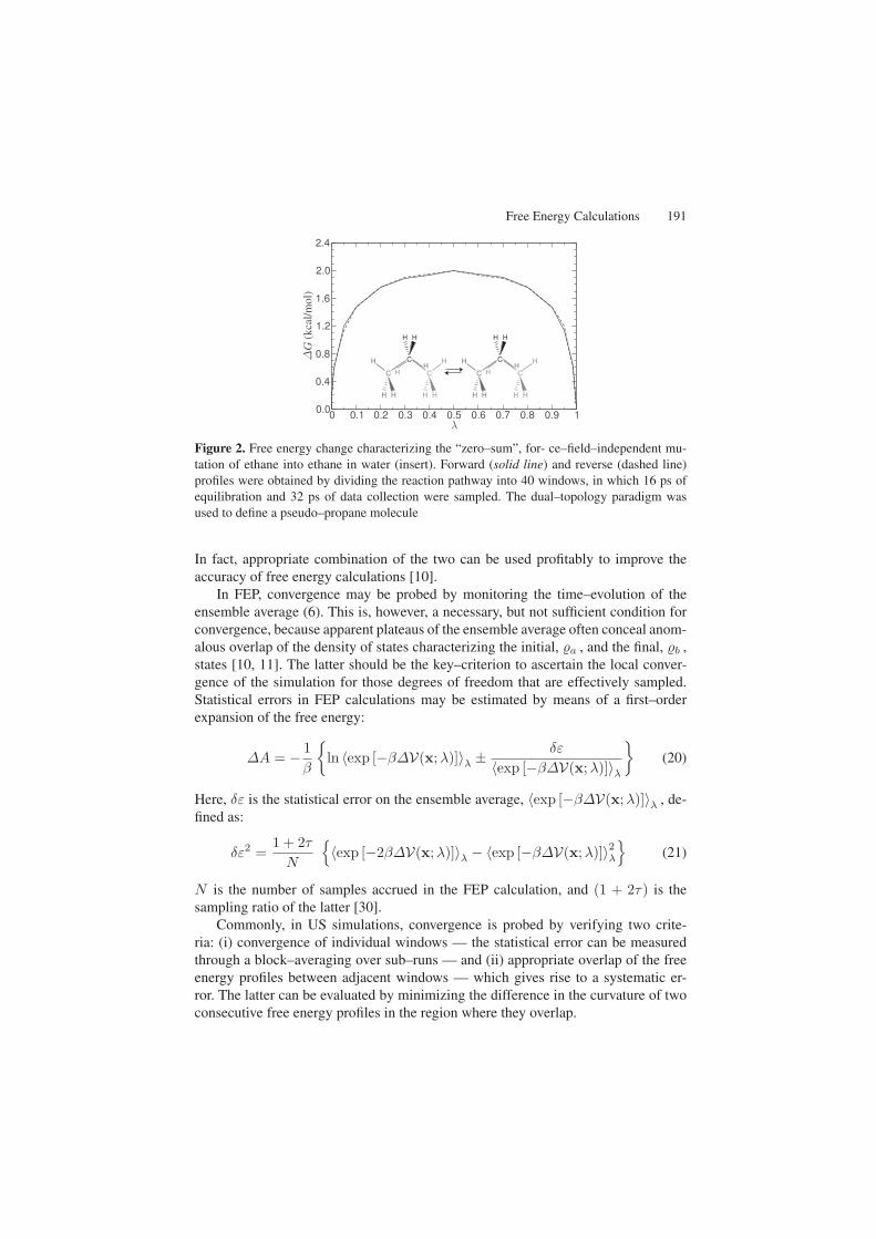
Appreciation of the statistical error has been devised following different schemes.Historically, the free energy changes for the λ → λ + δλ and the λ → λ − δλperturbations were computed simultaneously to provide the hysteresis between theforward and the reverse transformations. In practice, it can be shown that when δλis sufficiently small, the hysteresis of such “double–wide sampling” simulation [27]becomes negligible, irrespective of the amount of sampling generated in each win-dow — as would be the case in a “slow–growth” calculation [28]. A somewhat lessarguable point of view consists in performing the transformation in the forward,a → b , and in the reverse, b → a, directions. Micro–reversibility imposes that,in principle, ∆Ab→a = −∆Aa→b — see for instance Fig. 2. Unfortunately, forwardand reverse transformations do not necessarily share the same convergence proper-ties. Case in point, the insertion and deletion of a particle [29]: Whereas the formersimulation converges rapidly towards the expected excess chemical potential, thelatter never does. This shortcoming can be ascribed to the fact that configurationsin which a cavity does not exist where a real atom is present are never sampled. Interms of density of states, this scenario would translate into �a embracing �b entirely,thereby ensuring a proper convergence of the forward simulation, whereas the samecannot be said for the reciprocal, reverse transformation. Estimation of errors basedon forward and reverse simulations should, therefore, be considered with great care.


Figure 2. Free energy change characterizing the “zero–sum”, force–field–independent mu-tation of ethane into ethane in water (insert). Forward (solid line) and reverse (dashed line)profiles were obtained by dividing the reaction pathway into 40 windows, in which 16 ps ofequilibration and 32 ps of data collection were sampled. The dual–topology paradigm wasused to define a pseudo–propane molecule

In fact, appropriate combination of the two can be used profitably to improve theaccuracy of free energy calculations [10].

In FEP, convergence may be probed by monitoring the time–evolution of theensemble average (6). This is, however, a necessary, but not sufficient condition forconvergence, because apparent plateaus of the ensemble average often conceal anom-alous overlap of the density of states characterizing the initial, �a , and the final, �b ,states [10, 11]. The latter should be the key–criterion to ascertain the local conver-gence of the simulation for those degrees of freedom that are effectively sampled.Statistical errors in FEP calculations may be estimated by means of a first–orderexpansion of the free energy:

∆A = − 1β

{ln 〈exp [−β∆V(x;λ)]〉λ ± δε

〈exp [−β∆V(x;λ)]〉λ

}(20)

Here, δε is the statistical error on the ensemble average, 〈exp [−β∆V(x;λ)]〉λ , de-fined as:

δε2 =1 + 2τN

{〈exp [−2β∆V(x;λ)]〉λ − 〈exp [−β∆V(x;λ)]〉2λ

}(21)

N is the number of samples accrued in the FEP calculation, and (1 + 2τ) is thesampling ratio of the latter [30].

Commonly, in US simulations, convergence is probed by verifying two crite-ria: (i) convergence of individual windows — the statistical error can be measuredthrough a block–averaging over sub–runs — and (ii) appropriate overlap of the freeenergy profiles between adjacent windows — which gives rise to a systematic er-ror. The latter can be evaluated by minimizing the difference in the curvature of twoconsecutive free energy profiles in the region where they overlap.

192 C. Chipot

In the idealistic cases where a thermodynamic cycle can be defined — e.g. in-vestigation of the conformational equilibrium of a short peptide through the αR →C7ax → αL → β′ ≡ (β,C5, C7eq) → αR successive transformations — closureof the latter imposes that the sum of individual free energy contributions sum upto zero [31]. In principle, any deviation from this target should provide a valuableguidance to improve sampling efficiency. In practice, discrimination of the faultytransformation, or transformations, is cumbersome on account of possible mutualcompensation or cancellation of errors.

As has been commented on previously, visual inspection of �a and �b indicateswhether the free energy calculation has converged [10, 11]. Deficiencies in the over-lap of the two distributions is also suggestive of possible errors, but it should bekept in mind that approximations like (20) only reflect the statistical precision of thecomputation, and evidently do not account for fluctuations in the system occurringover long time scales. In sharp contrast, the statistical accuracy is expected to yield amore faithful picture of the degrees of freedom that have been actually sampled. Thesafest route to estimate this quantity consists in performing the same free energy cal-culation, starting from different regions of the phase space — viz. the error is definedas the root mean square deviation over the different simulations [32]. Semanticallyspeaking, the error measured from one individual run yields the statistical precisionof the free energy calculation, whereas that derived from the ensemble of simulationsprovides its statistical accuracy.

3 Free Energy Calculations and Drug Design

One of the grand challenges of free energy calculations is their ability to play apredictive role in ranking ligands of potential pharmaceutical interest, agonist or an-tagonist, according to their relative affinity towards a given protein. The usefulnessof such numerical simulations outside an academic environment can be assessed byanswering the following question: Can free energy calculations provide a convinc-ing answer faster than experiments are carried out in an industrial setting? Earlyencouraging results had triggered much excitement in the community, opening newvistas for de novo, rational drug design. They were, however, subsequently shatteredwhen it was realized that accurate free energies would require considerably morecomputational effort than was appreciated hitherto. Beyond the fundamental need ofappropriate sampling to yield converged ensemble averages — today, easily achiev-able in some favorable cases by means of inexpensive clusters of personal computers— the necessity of well–parameterized potential energy functions, suitable for non–peptide ligands, rapidly turns out to constitute a critical bottleneck for the routineuse of free energy calculations in the pharmaceutical industry. Closely related to theparametrization of the force field, setting up free energy calculations — i.e. defin-ing the alternate topology of the mutated moieties and the initial set of coordinates— is sufficiently time–consuming to be incompatible with the high–throughput re-quirements of industrial environments. In essence, this is where the paradox of freeenergy calculations lies: They have not yet come of age to be considered as black box


routine jobs, but should evolve in that direction to become part of the arsenal of com-putational tools available to the pharmaceutical industry. Selection of potent ligandcandidates in large data bases containing several millions of real or virtual mole-cules, employing a screening funnel that involves increasingly complex searchingtools, from crude geometrical recognition to more sophisticated flexible moleculardocking, offers new prospects for de novo drug design. In this pipeline of screeningmethods, free energy calculations should evidently be positioned at the very end,i.e. at the level of the optimization loop aimed at a limited number of ligands, whichalso checks adsorption–metabolism/toxicology (ADME/TOX) properties. Ideally, asselection in the funnel proceeds, the computational effort should remain constant —viz. the amount of CPU time necessary to perform free energy calculations on a fewcandidates is equivalent to that involved in the rough geometrical recognition over anumber of molecules five to six orders of magnitude larger.

Perhaps the key to the generalized and routine use of free energy calculationsfor molecular systems of pharmacological relevance is the demonstration that thismethodology can be applied fruitfully to problems that clearly go beyond the typi-cal scope of an academic environment. Collaborative projects with the pharmaceu-tical industry provide such a framework. In the context of the search for therapeuticagents targeted at osteoporosis and other bone–related diseases, free energy calcula-tions have been applied to complexes formed by the multi–domain protein pp60srckinase associated to non–peptide inhibitors. pp60src kinase is involved in signal trans-duction pathways and is implicated in osteoclast–mediated bone resorption [33]. Ofparticular interest, its SH2 domain, a common recognition motif of highly conservedprotein sequence, binds preferentially phosphotyrosine (pY)–containing peptides. Inmost circumstances, the latter adopt an extended conformation mimicking a two–pronged plug that interacts at two distinct anchoring sites of the protein — i.e. thehydrophilic phosphotyrosine pocket and the hydrophobic pocket — separated by aflat surface [34, 35]. For instance, the prototypical tetrapeptide pYEEI — a sequencefound on the PDGF receptor upon activation, appears to recognize the src SH2 do-main with an appropriate specificity.

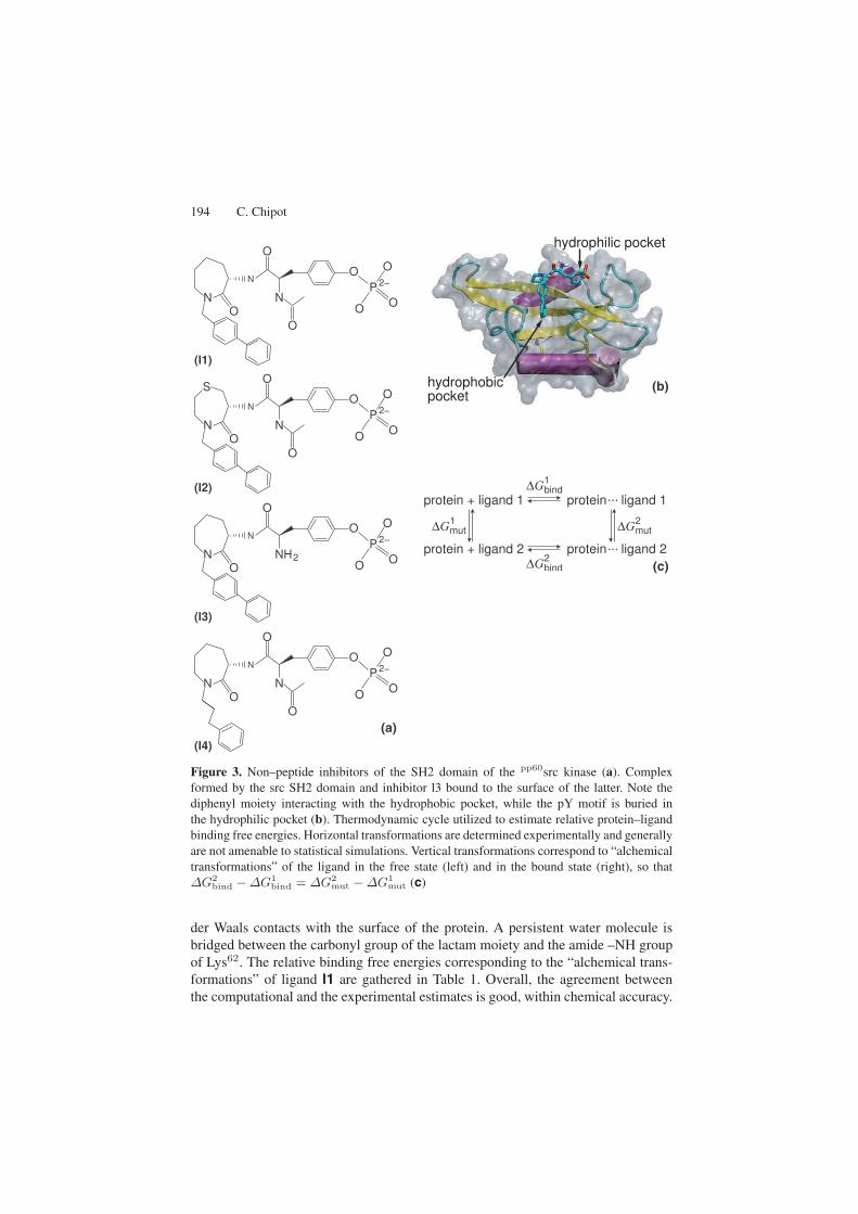
In silico point mutations have been performed on a series of non–peptide in-hibitors — see Fig. 3, using the FEP methodology in conjunction with the dual–topology paradigm. All simulations have been carried in the isothermal–isobaricensemble, using the program NAMD [36, 37]. The temperature and the pressurewere fixed at 300 K and 1 atm, respectively, employing Langevin dynamics and theLangevin piston. To avoid possible end–point catastrophes, 33 windows of unevenwidth, δλ , were utilized to scale the interaction of the mutated moieties with theirenvironment. The total length of each trajectory is equal to 1 ns, in the free and inthe bound states. Forward and reverse simulations were run to estimate the statisticalerror, with the assumption that the two transformations have identical convergenceproperties. The structures of the protein–ligand complex were determined by x–raycrystallography [34, 35].

Compared with pYEEI, ligand l1 adopts a very similar binding mode. Thebiphenyl moiety occupies the hydrophobic pocket entirely and the interaction of pYwith the hydrophilic site is strong. The scaffold of the peptide forms steady van

194 C. Chipot

(a)

(b)

(c)

Figure 3. Non–peptide inhibitors of the SH2 domain of the pp60src kinase (a). Complexformed by the src SH2 domain and inhibitor l3 bound to the surface of the latter. Note thediphenyl moiety interacting with the hydrophobic pocket, while the pY motif is buried inthe hydrophilic pocket (b). Thermodynamic cycle utilized to estimate relative protein–ligandbinding free energies. Horizontal transformations are determined experimentally and generallyare not amenable to statistical simulations. Vertical transformations correspond to “alchemicaltransformations” of the ligand in the free state (left) and in the bound state (right), so that∆G2

bind − ∆G1bind = ∆G2

mut − ∆G1mut (c)

der Waals contacts with the surface of the protein. A persistent water molecule isbridged between the carbonyl group of the lactam moiety and the amide –NH groupof Lys62. The relative binding free energies corresponding to the “alchemical trans-formations” of ligand l1 are gathered in Table 1. Overall, the agreement betweenthe computational and the experimental estimates is good, within chemical accuracy.


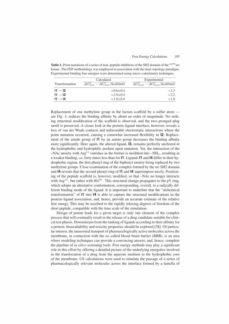
Table 1. Point mutations of a series of non–peptide inhibitors of the SH2 domain of the pp60srckinase. The FEP methodology was employed in association with the dual–topology paradigm.Experimental binding free energies were determined using micro–calorimetry techniques

Calculated ExperimentalTransformation ∆G2

mut − ∆G1mut (kcal/mol) ∆G2

bind − ∆G1bind (kcal/mol)

l1 → l2 +0.6±0.4 +1.3l1 → l3 +2.9±0.4 +2.2l1 → l4 +1.9±0.4 +1.8

Replacement of one methylene group in the lactam scaffold by a sulfur atom —see Fig. 3, reduces the binding affinity by about an order of magnitude. No strik-ing structural modification of the scaffold is observed, and the two–pronged plugmotif is preserved. A closer look at the protein–ligand interface, however, reveals aloss of van der Waals contacts and unfavorable electrostatic interactions where thepoint mutation occurred, causing a somewhat increased flexibility in l2. Replace-ment of the amide group of l1 by an amino group decreases the binding affinitymore significantly. Here again, the altered ligand, l3, remains perfectly anchored inthe hydrophobic and hydrophilic pockets upon mutation. Yet, the interaction of the–NAc moiety with Arg14 vanishes as the former is modified into –NH2 , resulting ina weaker binding, ca. forty times less than for l1. Ligands l1 and l4 differ in their hy-drophobic region, the first phenyl ring of the biphenyl moiety being replaced by twomethylene groups. Close examination of the complex formed by the src SH2 domainand l4 reveals that the second phenyl ring of l1 and l4 superimpose nicely. Position-ing of the peptide scaffold is, however, modified, so that –NAc no longer interactswith Arg14 , but rather with His60 . This structural change propagates to the pY ring,which adopts an alternative conformation, corresponding, overall, to a radically dif-ferent binding mode of the ligand. It is important to underline that the “alchemicaltransformation” of l1 into l4 is able to capture the structural modifications in theprotein–ligand association, and, hence, provide an accurate estimate of the relativefree energy. This may be ascribed to the rapidly relaxing degrees of freedom of theshort peptide, compatible with the time scale of the simulation.

Design of potent leads for a given target is only one element of the complexprocess that will eventually result in the release of a drug candidate suitable for clini-cal test phases. Downstream from the ranking of ligands according to their affinity fora protein, bioavailability and toxicity properties should be explored [38]. Of particu-lar interest, the unassisted transport of pharmacologically active molecules across themembrane, in connection with the so–called blood–brain barrier (BBB), is an areawhere modeling techniques can provide a convincing answer, and, hence, completethe pipeline of in silico screening tools. Free energy methods may play a significantrole in this effort by offering a detailed picture of the underlying energetics involvedin the translocation of a drug from the aqueous medium to the hydrophobic coreof the membrane. US calculations were used to simulate the passage of a series ofpharmacologically relevant molecules across the interface formed by a lamella of

196 C. Chipot

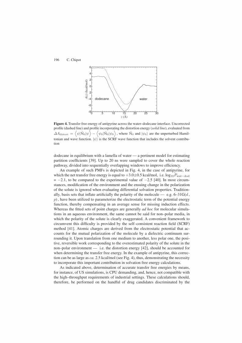
Figure 4. Transfer free energy of antipyrine across the water–dodecane interface. Uncorrectedprofile (dashed line) and profile incorporating the distortion energy (solid line), evaluated from

∆Adistort =⟨ψ|H0|ψ

⟩−

⟨ψ0|H0|ψ0

⟩, where H0 and |ψ0〉 are the unperturbed Hamil-

tonian and wave function. |ψ〉 is the SCRF wave function that includes the solvent contribu-tion

dodecane in equilibrium with a lamella of water — a pertinent model for estimatingpartition coefficients [39]. Up to 20 ns were sampled to cover the whole reactionpathway, divided into sequentially overlapping windows to improve efficiency.

An example of such PMFs is depicted in Fig. 4, in the case of antipyrine, forwhich the net transfer free energy is equal to +3.0±0.5 kcal/mol, i.e. log10Pwat−dod

= −2.1, to be compared to the experimental value of −2.5 [40]. In most circum-stances, modification of the environment and the ensuing change in the polarizationof the solute is ignored when evaluating differential solvation properties. Tradition-ally, basis sets that inflate artificially the polarity of the molecule — e.g. 6–31G(d ,p) , have been utilized to parameterize the electrostatic term of the potential energyfunction, thereby compensating in an average sense for missing induction effects.Whereas the fitted sets of point charges are generally ad hoc for molecular simula-tions in an aqueous environment, the same cannot be said for non–polar media, inwhich the polarity of the solute is clearly exaggerated. A convenient framework tocircumvent this difficulty is provided by the self–consistent reaction field (SCRF)method [41]. Atomic charges are derived from the electrostatic potential that ac-counts for the mutual polarization of the molecule by a dielectric continuum sur-rounding it. Upon translation from one medium to another, less polar one, the posi-tive, reversible work corresponding to the overestimated polarity of the solute in thenon–polar environment — i.e. the distortion energy [42], should be accounted forwhen determining the transfer free energy. In the example of antipyrine, this correc-tion can be as large as ca. 2.5 kcal/mol (see Fig. 4), thus, demonstrating the necessityto incorporate this important contribution in solvation free energy calculations.

As indicated above, determination of accurate transfer free energies by means,for instance, of US simulations, is CPU demanding, and, hence, not compatible withthe high–throughput requirements of industrial settings. These calculations should,therefore, be performed on the handful of drug candidates discriminated by the


screening process. Faster approaches have been devised, however, based on quan-tum chemical calculations associated to an SCRF scheme for taking solvent effectsinto account. Aside from the electrostatic term, van der Waals contributions are usu-ally evaluated from empirical formulation using the solvent accessible surface area(SASA) of the solute. This set of methods is substantially faster than statistical sim-ulations, but, at the same time, only supply simple liquid–liquid partition coeffi-cients, rather than the full free energy behavior characterizing the translocation ofthe molecule between the two media. This information may, however, turn out to beof paramount importance to rationalize biological phenomena. Such was the case, forinstance, of general anesthesia by inhaled anesthetics, an interfacial process shownto result from the accumulation of anesthetics at the water–membrane interface ofneuronal tissues [43].

4 Free Energy Calculations and Signal Transduction

The paucity of structural information available for membrane proteins has imparteda new momentum in the in silico investigation of these systems. The grand challengeof molecular modeling is to attain the microscopic detail that is often inaccessible toconventional experimental techniques. Of topical interest are seven transmembrane(TM) domain G–protein coupled receptors (GPCRs) [44], which correspond to thethird largest family of genes in the human genome, and, therefore, represent privi-leged targets for de novo drug design. Full resolution by x–ray crystallography of thethree–dimensional structure of bovine rhodopsin [45], the only GPCR structure tothis date, has opened new vistas for the modeling of related membrane proteins. Un-fortunately, crystallization of this receptor in its dark, inactive state precludes the useof the structure for homology modeling of GPCR–ligand activated complexes [46].When neither theory nor experiment can provide atomic–level, three–dimensionalstructures of GPCRs, their synergistic combination offers an interesting perspectiveto reach this goal. Such a self–consistent strategy between experimentalists and mod-elers has been applied successfully to elucidate the structure of the human receptor ofcholecystokinin (CCK1R) in the presence of an agonist ligand [47] — viz. a nonapep-tide (CCK9) [48] of sequence Arg–Asp–S-Tyr–Thr–Gly–Trp–Met–Asp–Phe–NH2 ,where S-Tyr stands for a sulfated tyrosyl amino acid. On the road towards a con-sistent in vacuo construction of the complex, site–directed mutagenesis experimentswere designed to pinpoint key receptor–ligand interactions, thereby helping in theplacement of TM α–helices and the docking of CCK9.

Whereas in vacuo models reflect the geometrical constraints enforced in thecourse of their construction, it is far from clear whether they will behave as ex-pected when immersed in a realistic membrane environment. Accordingly, the modelformed by CCK1R and CC9 was inserted in a fully hydrated palmitoyloleylphos-phatidylcholine (POPC) bilayer, resulting in a system of 72,255 atoms, and the com-plete assembly was probed in a 10.5 ns MD simulation. Analysis of the trajectoryreveals no apparent loss of secondary structure in the TM domain, and a distance rootmean square deviation for the backbone atoms not exceeding 2 Å. More importantly,

198 C. Chipot

the crucial receptor–ligand interactions are preserved throughout the simulation —e.g. Arg336 with Asp8 [49], and Met195 and Arg197 with S-Tyr3 [50, 51]. Admit-tedly, such numerical experiments in essence only supply a qualitative picture of thestructural properties of the molecular assembly and its integrity over the time scaleexplored. Free energy calculations go one step beyond by quantifying intermolecu-lar interactions according to their importance, and, consequently, represent a tangiblethermodynamic measure for assessing the accuracy of the model. Furthermore, thisinformation is directly comparable to site–directed mutagenesis experiments utilizedin the in vacuo construction of the receptor, thereby closing the loop of the modelingprocess.

To some extent, performing free energy calculations in such large molecular as-semblies may be viewed as a bold and perhaps foolish leap of faith, considering thevarious possible sources of errors likely to affect the final result. Among the latter,attempting to reproduce free energy differences using a three–dimensional model inlieu of a well–resolved, experimentally determined structure casts the greatest doubtson the chances of success of this venture. Of equal concern, “alchemical transforma-tions” involving charged amino acids are driven primarily by the solvation of theionic moieties, resulting in large free energies, the difference of which, between thefree and the bound states, is expected to be small. Assuming a validated model, whichappears to be confirmed by the preliminary MD simulation, a key–question, alreadymentioned in this chapter, remains: When is “enough sampling” really enough? Thisconundrum should be, in fact, rephrased here as: Are the time scales characteristicof the slowest degrees of freedom in the system crucial for the free energy changesthat are being estimated? For instance, is the mutation of the penultimate amino acidof CCK9 — viz. Asp8 into alanine (see Fig. 5), likely to be affected by the slow col-lective motions of lipid molecules, or possible vertical and lateral motions of TM α–helices? Nanosecond MD simulations obviously cannot capture these events, whichoccur over significantly longer times. Yet, under the assumption that the replacementof an agonist ligand by an alternate one does not entail any noticeable rearrangementof the TM domain, current free energy calculations are likely to be appropriate forranking ligands according to their affinity towards a given GPCR.

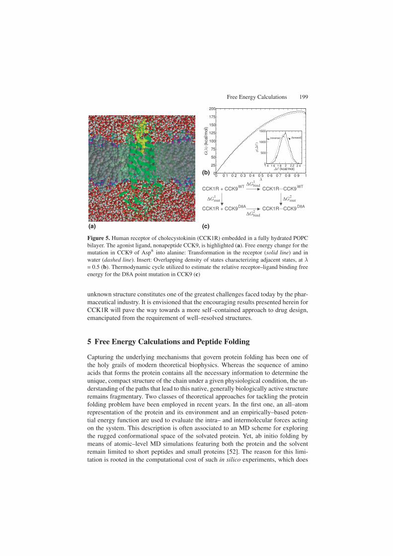
The FEP estimate of +3.1±0.7 kcal/mol for the D8A transformation agrees, in-deed, very well with the site–directed mutagenesis experiments that yielded a free en-ergy change equal to +3.6 kcal/mol. The in silico value was obtained from two runsof 3.4 ns each, in bulk water and in CCK1R, respectively, breaking the reaction pathinto 114 consecutive windows of uneven width, and using the dual–topology para-digm. The error was estimated from two distinct runs performed at 5.0 and 10.5 ns ofthe MD simulation. In contrast with an error derived from a first–order expansion ofthe free energy, which only reflects the statistical precision of the calculation — here,±0.3 kcal/mol, repeating the simulation from distinct initial conditions accounts forfluctuations of the structure over longer time scales. Put together, while it is difficultto ascertain without ambiguity the correctness of the three–dimensional structure inthe sole light of a limited number of numerical experiments, it still remains that thehost of observations accrued in theses simulations coincide nicely with the collec-tion of experimental data. De novo development of new drug candidates for targets of


(b)

(a) (c)

Figure 5. Human receptor of cholecystokinin (CCK1R) embedded in a fully hydrated POPCbilayer. The agonist ligand, nonapeptide CCK9, is highlighted (a). Free energy change for themutation in CCK9 of Asp8 into alanine: Transformation in the receptor (solid line) and inwater (dashed line). Insert: Overlapping density of states characterizing adjacent states, at λ= 0.5 (b). Thermodynamic cycle utilized to estimate the relative receptor–ligand binding freeenergy for the D8A point mutation in CCK9 (c)

unknown structure constitutes one of the greatest challenges faced today by the phar-maceutical industry. It is envisioned that the encouraging results presented herein forCCK1R will pave the way towards a more self–contained approach to drug design,emancipated from the requirement of well–resolved structures.

5 Free Energy Calculations and Peptide Folding

Capturing the underlying mechanisms that govern protein folding has been one ofthe holy grails of modern theoretical biophysics. Whereas the sequence of aminoacids that forms the protein contains all the necessary information to determine theunique, compact structure of the chain under a given physiological condition, the un-derstanding of the paths that lead to this native, generally biologically active structureremains fragmentary. Two classes of theoretical approaches for tackling the proteinfolding problem have been employed in recent years. In the first one, an all–atomrepresentation of the protein and its environment and an empirically–based poten-tial energy function are used to evaluate the intra– and intermolecular forces actingon the system. This description is often associated to an MD scheme for exploringthe rugged conformational space of the solvated protein. Yet, ab initio folding bymeans of atomic–level MD simulations featuring both the protein and the solventremain limited to short peptides and small proteins [52]. The reason for this limi-tation is rooted in the computational cost of such in silico experiments, which does

200 C. Chipot

not allow biologically relevant time scales to be accessed routinely. An alternativeto the detailed, all–atom approach consists in turning to somewhat rougher models,that, nonetheless, retain the fundamental characteristics of protein chains. Such isthe case of coarse–grained models, in which each amino acid of the protein is repre-sented by a bead located at the vertex of a two– or a three–dimensional lattice [53].An intermediate description consists of an all–atom representation of the protein inan implicit solvent. It is far from clear, however, whether the delicate interplay of theprotein with explicit water molecules is a necessary condition for guaranteeing thecorrect folding toward the native state.

Whereas MD simulations involving an explicit solvent rarely exceed a few hun-dreds of ns [54], significantly shorter free energy calculations can be designed ad-vantageously to understand the physical phenomena that drive folding. Among thesephenomena, the subtle, temperature–dependent hydrophobic effect [55, 56] remainsone of the most investigated to rationalize the collapse of a disordered protein chaininto an appropriately folded one. The choice of a pertinent reaction coordinate thatcharacterizes the folding process of a short peptide, let alone a small protein, con-stitutes a conundrum, unlikely to find a definitive answer in the near future. Thisintricate problem is rooted in the vast number of degrees of freedom that vary con-comitantly as the peptide evolves toward a folded structure. The free energy is, there-fore, a function of many variables that cannot be accounted for in a straightforwardfashion. Valuable information may, nonetheless, be obtained from simple model sys-tems, for which a non–ambiguous reaction coordinate can be defined. Such is thecase of the terminally blocked undecamer of L–leucine organized in an α–helix, theC–terminal residue of which was unfolded from an α–helical conformation to thatof a β–strand [57]. Similar calculations have been endeavored with blocked poly–L–alanine of various lengths to examine helix propagation at its N– and C–termini [58]

To highlight the temperature–dependent nature of the hydrophobic effect, the MDsimulations were run in the canonical ensemble at 280, 300, 320, 340, 360 and 370 K,using the Nosé–Hoover algorithm implemented in the program COSMOS. Changesin the free energy consecutive to modifications of the last ψ dihedral angle of thehomopolypeptide were estimated with the US method. All other torsional angleswere restrained softly in a range characteristic of an α–helix. For each temperature,the complete reaction pathway connecting the α–helical state to the β–strand —roughly speaking −90 ≤ ψ ≤ +170◦ , was broken down in five mutually overlappingwindows. The full free energy profiles were subsequently reconstructed employingWHAM. The total simulation length varied from 14 ns at 370 K, to 76 ns at 280 K,on account of the slower relaxation at lower temperatures.

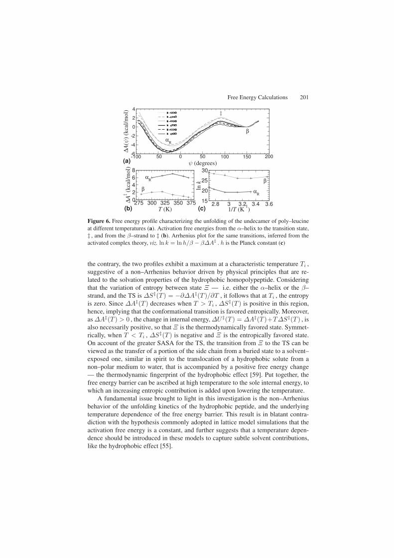
The PMFs shown in Fig. 6 each possess two distinct local minima correspondingto the α–helix and the β–strand, and separated by a maximum of the free energyaround 90◦ . These three conformational states are characterized by different SASAs— viz. 134±2, 149±7 and 117±13 Å2 for the α–helix, the transition state (TS) andthe β–strand, respectively. The most striking feature of the PMFs lies in the tempera-ture dependence of the free energy associated to the transition from the α–helix to theTS, ∆AαR→‡ , and that from the β–strand to the TS, ∆Aβ→‡ . Furthermore, neither∆AαR→‡(T ) nor ∆Aβ→‡(T ) varies monotonically as the temperature increases. On


Figure 6. Free energy profile characterizing the unfolding of the undecamer of poly–leucineat different temperatures (a). Activation free energies from the α–helix to the transition state,‡ , and from the β–strand to ‡ (b). Arrhenius plot for the same transitions, inferred from theactivated complex theory, viz. ln k = ln h/β − β∆A‡ . h is the Planck constant (c)

the contrary, the two profiles exhibit a maximum at a characteristic temperature Ti ,suggestive of a non–Arrhenius behavior driven by physical principles that are re-lated to the solvation properties of the hydrophobic homopolypeptide. Consideringthat the variation of entropy between state Ξ — i.e. either the α–helix or the β–strand, and the TS is ∆S‡(T ) = −∂∆A‡(T )/∂T , it follows that at Ti , the entropyis zero. Since ∆A‡(T ) decreases when T > Ti , ∆S‡(T ) is positive in this region,hence, implying that the conformational transition is favored entropically. Moreover,as ∆A‡(T ) > 0 , the change in internal energy, ∆U‡(T ) = ∆A‡(T )+T∆S‡(T ) , isalso necessarily positive, so that Ξ is the thermodynamically favored state. Symmet-rically, when T < Ti , ∆S‡(T ) is negative and Ξ is the entropically favored state.On account of the greater SASA for the TS, the transition from Ξ to the TS can beviewed as the transfer of a portion of the side chain from a buried state to a solvent–exposed one, similar in spirit to the translocation of a hydrophobic solute from anon–polar medium to water, that is accompanied by a positive free energy change— the thermodynamic fingerprint of the hydrophobic effect [59]. Put together, thefree energy barrier can be ascribed at high temperature to the sole internal energy, towhich an increasing entropic contribution is added upon lowering the temperature.

A fundamental issue brought to light in this investigation is the non–Arrheniusbehavior of the unfolding kinetics of the hydrophobic peptide, and the underlyingtemperature dependence of the free energy barrier. This result is in blatant contra-diction with the hypothesis commonly adopted in lattice model simulations that theactivation free energy is a constant, and further suggests that a temperature depen-dence should be introduced in these models to capture subtle solvent contributions,like the hydrophobic effect [55].

202 C. Chipot

6 Free Energy Calculations and Membrane Protein Association

To a large extent, our knowledge of how membrane protein domains recognize andassociate into functional, three–dimensional entities remains fragmentary. Whereasthe structure of membrane proteins can be particularly complex, their TM regionis often simple, consisting in general of a bundle of α–helices, or barrels of β–strands. An important result brought to light by deletion experiments indicates thatsome membrane proteins can retain their biological function upon removal of largefractions of the protein. This is suggestive that rudimentary models, like simple α–helices, can be utilized to understand the recognition and association processes ofTM segments into complex membrane proteins. On the road to reach this goal, the“two–stage” model [60] provides an interesting view for rationalizing the folding ofmembrane proteins. According to this model, elements of the secondary structure— viz. in most cases, α–helices, are first formed and inserted into the lipid bilayer,prior to specific inter–helical interactions that drive the TM segments towards well–ordered, native structures. Capturing the atomic detail of the underlying mechanismsresponsible for α–helix recognition and association requires model systems that aresupported by robust experimental data to appraise the accuracy of the computationsendeavored. Glycophorin A (GpA), a glycoprotein ubiquitous to the human erythro-cyte membrane, represents one such system. It forms non–covalent dimers throughthe reversible association of its membrane–spanning domain — i.e. residues 62 to101, albeit only residues 73 to 96 actually adopt an α–helical conformation [61–63].Inter–helical association has been shown to result from specific interactions involv-ing a heptad of residues, essentially located on one face of each TM segment, as maybe seen in Fig. 7.

(a) (b)

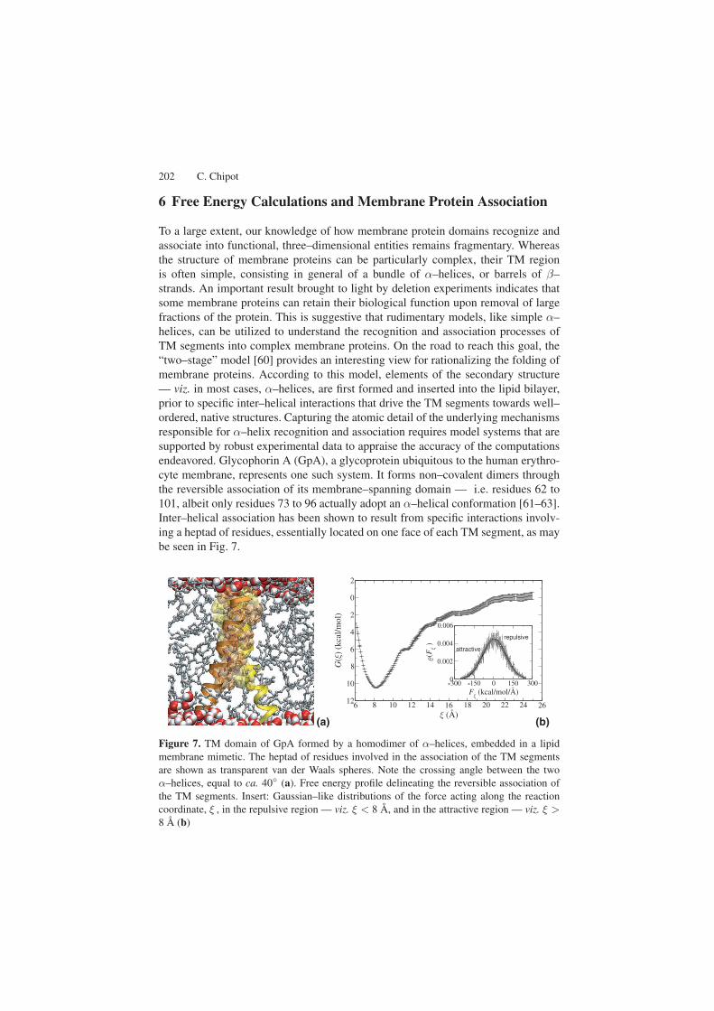
Figure 7. TM domain of GpA formed by a homodimer of α–helices, embedded in a lipidmembrane mimetic. The heptad of residues involved in the association of the TM segmentsare shown as transparent van der Waals spheres. Note the crossing angle between the twoα–helices, equal to ca. 40◦ (a). Free energy profile delineating the reversible association ofthe TM segments. Insert: Gaussian–like distributions of the force acting along the reactioncoordinate, ξ , in the repulsive region — viz. ξ < 8 Å, and in the attractive region — viz. ξ >8 Å (b)


The reversible association of GpA in a lipid bilayer was modelled using itsdimeric, α–helical TM segments immersed in a membrane mimetic formed by alamella of dodecane placed between two lamellae of water. The ABF method in-troduced in the program NAMD [26] was employed to allow the TM segments todiffuse freely along the reaction coordinate, ξ , chosen to be the distance separatingthe centers of mass of the two α–helices. Such a free energy calculation is not onlychallenging methodologically, but it is also of paramount importance from a biophys-ical standpoint, because it bridges structural data obtained from nuclear magneticresonance (NMR) [61–63] to thermodynamic data obtained from analytical ultra-centrifugation [64, 65] and fluorescence resonance energy transfer (FRET) [66, 67],providing a dynamic view of the recognition and association stages.

Visual inspection of the PMF derived from a 125 ns simulation and describingthe reversible association of the α–helices reveals a qualitatively simple profile, fea-turing a single minimum characteristic of the native, dimeric state. As ξ increases, sodoes the free energy, progressing by steps that correspond to the successive breakingof inter–helical contacts. Beyond 21 Å, the TM segments are sufficiently separatedto assume that they no longer interact. Integration of the PMF in the limit of α–helixassociation yields the association constant and, hence, the free energy of dimeriza-tion, equal to +11.5±0.4 kcal/mol. Direct and precise comparison of this value withexperiment is not possible, because measurements were carried in different environ-ments, namely hydrocarbon vs.detergent micelles. It can, nonetheless, be inferredthat the value in dodecane probably constitutes an upper bound to the experimentalestimates determined in micelles, on account of (i) the greater order imposed by thedetergent chains, and, (ii) the hydrophobic fraction of the system that increases withthe length of the chain [67].

Deconvolution of the PMF into free energy components illuminates two distinctregimes controlling recognition and association. At large separations, as inter–helicalcontacts vanish, the helix–helix term becomes progressively negligible, resulting es-sentially from the interaction of two macro–dipoles. The TM segments are stabilizedby favorable helix–solvent contributions. In contrast, at short separations, helix–helixinteractions are prominent and govern the change in the free energy near the globalminimum. Association proceeds through the transient formation of early, non–nativecontacts involving residues that act as recognition sites. These contacts are subse-quently replaced by contacts in the heptad of residues responsible for association,concomitantly with the tilt of the two α–helices from an upright position to thatcharacteristic of the native dimer.

7 Conclusion

Free energy calculations constitute a tangible link between theory and experiment, byquantifying at the thermodynamic level the physical phenomena modelled by statis-tical simulations. With twenty years of hindsight gained from methodological devel-opment and characterization, a variety of problems of both chemical and biologicalrelevance can now be tackled with confidence. Among the progresses achieved in

204 C. Chipot

recent years, a significant step forward has been made in the calculation of free en-ergies along a reaction coordinate, in particular employing the concept of an averageforce acting along this coordinate [25, 26]. “Alchemical transformations” utilized tomimic site–directed mutagenesis experiments have also benefited from advances inthe understanding of the methodology and how the latter should be applied [68]. Ef-forts to characterize and estimate the error affecting the simulations [10, 11, 69] haveequally played an active role in turning free energy calculations into another tool inthe arsenal of computational methods available to the modeler. Put together, freeenergy calculations have come of age to become a predictive approach, instead ofremaining at the stage of a mere proof of concept [70]. As has been illustrated in thischapter, they can be applied to numerous problems, ranging from de novo drug de-sign to the understanding of biophysical processes in lipid membranes. Free energycalculations, however, cannot yet be considered as “black box”, routine jobs. A ro-bust, reliable methodology does not necessarily imply that it can be used blindly. Thenature of the problem dictates the choice of the method and the associated protocol— e.g. US vs.FEP vs.TI vs.average force, the number of intermediate λ–states alonga reaction coordinate, the pertinent choice of this reaction coordinate, the amount ofsampling per individual λ–state, a single vs.a dual topology paradigm for “alchemi-cal transformations”, or constrained vs.unconstrained MD. Furthermore, little efforthas been hitherto devoted to the automatization of free energy calculations, through,for instance, a user–friendly definition of the topologies representative of the initialand the final states of a transformation. With the increased access to massively par-allel architectures as the price/performance ratio of computer chips continues to fallinexorably, the bottleneck of free energy calculations has shifted from a purely com-putational aspect to a human one, due to the need of qualified modelers to set thesecalculations up. This explains why their use in industry, and particularly in the phar-maceutical world, over the past years has remained scarce. Cutting–edge applicationsof free energy calculations emanate essentially from academic environments, wherethe focus is not so much on high throughput, but rather on well–delineated, specificproblems that often require more human attention than computational power. Yet,it is envisioned that in a reasonably near future, free energy methods will becomean unavoidable element of screening pipelines, discriminating between candidatesselected from cruder approaches, to retain only the best leads towards a given target.

Acknowledgments

Jérôme Hénin, Surjit Dixit, Olivier Collet, Eric Darve, Andrew Pohorille and AlanE. Mark are gratefully acknowledged for fruitful and inspiring discussions. The au-thor thank the Centre Informatique National de l’Enseignement Supérieur (CINES)and the centre de Calcul Réseaux et Visualisation Haute Performance (CRVHP) forgenerous provision of CPU time on their SGI Origin 3000 architectures.


References

[1] Kollman, P. A., Free energy calculations: Applications to chemical and bio-chemical phenomena, Chem. Rev. 93, 2395–2417, 1993.

[2] Postma, J. P. M.; Berendsen, H. J. C.; Haak, J. R., Thermodynamics of cavityformation in water: A molecular dynamics study, Faraday Symp. Chem. Soc.17, 55–67, 1982.

[3] Warshel, A., Dynamics of reactions in polar solvents. Semiclassical trajectorystudies of electron transfer and proton transfer reactions, J. Phys. Chem. 86,2218–2224, 1982.

[4] Bash, P. A.; Singh, U. C.; Langridge, R.; Kollman, P. A., Free energy calcula-tions by computer simulation, Science 236, 564–568, 1987.

[5] Bash, P. A.; Singh, U. C.; Brown, F. K.; Langridge, R.; Kollman, P. A., Cal-culation of the relative change in binding free energy of a protein–inhibitorcomplex, Science 235, 574–576, 1987.

[6] McQuarrie, D. A., Statistical mechanics, Harper and Row: New York, 1976.[7] Allen, M. P.; Tildesley, D. J., Computer Simulation of Liquids, Clarendon Press:

Oxford, 1987.[8] Kirkwood, J. G., Statistical mechanics of fluid mixtures, J. Chem. Phys. 3,

300–313, 1935.[9] Zwanzig, R. W., High–temperature equation of state by a perturbation method.

I. Nonpolar gases, J. Chem. Phys. 22, 1420–1426, 1954.[10] Lu, N.; Singh, J. K.; Kofke, D. A.; Woolf, T. B., Appropriate methods to com-

bine forward and reverse free–energy perturbation averages, J. Chem. Phys.118, 2977–2984, 2003.

[11] Lu, N.; Kofke, D. A.; Woolf, T. B., Improving the efficiency and reliabilityof free energy perturbation calculations using overlap sampling methods, J.Comput. Chem. 25, 28–39, 2004.

[12] Mark, A. E. Free Energy Perturbation Calculations. in Encyclopedia of com-putational chemistry, Schleyer, P. v. R.; Allinger, N. L.; Clark, T.; Gasteiger,J.; Kollman, P. A.; Schaefer III, H. F.; Schreiner, P. R., Eds., vol. 2. Wiley andSons, Chichester, 1998, pp. 1070–1083.

[13] Torrie, G. M.; Valleau, J. P., Nonphysical sampling distributions in Monte Carlofree energy estimation: Umbrella sampling, J. Comput. Phys. 23, 187–199,1977.

[14] Pearlman, D. A.; Kollman, P. A., The overlooked bond–stretching contributionin free energy perturbation calculations, J. Chem. Phys. 94, 4532–4545, 1991.

[15] Boresch, S.; Karplus, M., The role of bonded terms in free energy simulations:I. Theoretical analysis, J. Phys. Chem. A 103, 103–118, 1999.

[16] Boresch, S.; Karplus, M., The role of bonded terms in free energy simulations:II. Calculation of their influence on free energy differences of solvation, J. Phys.Chem. A 103, 119–136, 1999.

[17] Pearlman, D. A., A comparison of alternative approaches to free energy calcu-lations, J. Phys. Chem. 98, 1487–1493, 1994.

206 C. Chipot

[18] Beutler, T. C.; Mark, A. E.; van Schaik, R. C.; Gerber, P. R.; van Gunsteren,W. F., Avoiding singularities and neumerical instabilities in free energy calcu-lations based on molecular simulations, Chem. Phys. Lett. 222, 529–539, 1994.

[19] Straatsma, T. P.; Berendsen, H. J. C., Free energy of ionic hydration: Analysisof a thermodynamic integration technique to evaluate free energy differencesby molecular dynamics simulations, J. Chem. Phys. 89, 5876–5886, 1988.

[20] Chandler, D., Introduction to modern statistical mechanics, Oxford UniversityPress, 1987.

[21] Kumar, S.; Bouzida, D.; Swendsen, R. H.; Kollman, P. A.; Rosenberg, J. M.,The weighted histogram analysis method for free energy calculations on bio-molecules. I. The method, J. Comput. Chem. 13, 1011–1021, 1992.

[22] Pearlman, D. A., Determining the contributions of constraints in free energycalculations: Development, characterization, amnd recommendations, J. Chem.Phys. 98, 8946–8957, 1993.

[23] den Otter, W. K.; Briels, W. J., The calculation of free–energy differences byconstrained molecular dynamics simulations, J. Chem. Phys. 109, 4139–4146,1998.

[24] den Otter, W. K., Thermodynamic integration of the free energy along a re-action coordinate in Cartesian coordinates, J. Chem. Phys. 112, 7283–7292,2000.

[25] Darve, E.; Pohorille, A., Calculating free energies using average force, J. Chem.Phys. 115, 9169–9183, 2001.

[26] Hénin, J.; Chipot, C., Overcoming free energy barriers using unconstrainedmolecular dynamics simulations, J. Chem. Phys. 121, 2904–2914, 2004.

[27] Jorgensen, W. L.; Ravimohan, C., Monte Carlo simulation of differences in freeenergies of hydration, J. Chem. Phys. 83, 3050–3054, 1985.

[28] Chipot, C.; Kollman, P. A.; Pearlman, D. A., Alternative approaches to potentialof mean force calculations: Free energy perturbation versus thermodynamic in-tegration. Case study of some representative nonpolar interactions, J. Comput.Chem. 17, 1112–1131, 1996.

[29] Widom, B., Some topics in the theory of fluids, J. Chem. Phys. 39, 2808–2812,1963.

[30] Straatsma, T. P.; Berendsen, H. J. C.; Stam, A. J., Estimation of statistical errorsin molecular simulation calculations, Mol. Phys. 57, 89–95, 1986.

[31] Chipot, C.; Pohorille, A., Conformational equilibria of terminally blocked sin-gle amino acids at the water–hexane interface. A molecular dynamics study, J.Phys. Chem. B 102, 281–290, 1998.

[32] Chipot, C.; Millot, C.; Maigret, B.; Kollman, P. A., Molecular dynamics freeenergy perturbation calculations. Influence of nonbonded parameters on thefree energy of hydration of charged and neutral species, J. Phys. Chem. 98,11362–11372, 1994.

[33] Soriano, P.; Montgomery, C.; Geske, R.; Bradley, A., Targeted disruption of thec–src proto–oncogene leads to osteopetrosis in mice., Cell 64, 693–702, 1991.

[34] Lange, G.; Lesuisse, D.; Deprez, P.; Schoot, B.; Loenze, P.; Benard, D.; Mar-quette, J. P.; Broto, P.; Sarubbi, E.; Mandine, E., Principles governing the


binding of a class of non–peptidic inhibitors to the SH2 domain of src stud-ied by X-ray analysis, J. Med. Chem. 45, 2915–2922, 2002.

[35] Lange, G.; Lesuisse, D.; Deprez, P.; Schoot, B.; Loenze, P.; Benard, D.; Mar-quette, J. P.; Broto, P.; Sarubbi, E.; Mandine, E., Requirements for specific bind-ing of low affinity inhibitor fragments to the SH2 domain of pp60Src are iden-tical to those for high affinity binding of full length inhibitors, J. Med. Chem.46, 5184–5195, 2003.

[36] Kale, L.; Skeel, R.; Bhandarkar, M.; Brunner, R.; Gursoy, A.; Krawetz, N.;Phillips, J.; Shinozaki, A.; Varadarajan, K.; Schulten, K., NAMD2: Greater scal-ability for parallel molecular dynamics, J. Comput. Phys. 151, 283–312, 1999.

[37] Bhandarkar, M.; Brunner, R.; Chipot, C.; Dalke, A.; Dixit, S.; Grayson, P.;Gullingsrud, J.; Gursoy, A.; Humphrey, W.; Hurwitz, D. et al. NAMD usersguide, version 2.5. Theoretical biophysics group, University of Illinois andBeckman Institute, 405 North Mathews, Urbana, Illinois 61801, September2003.

[38] Carrupt, P.; Testa, B.; Gaillard, P. Computational approaches to lipophilicity:Methods and applications. in Reviews in Computational Chemistry, Lipkowitz,K.; Boyd, D. B., Eds., vol. 11. VCH, New York, 1997, pp. 241–345.

[39] Wohnsland, F.; Faller, B., High–throughput permeability pH profile and high–throughput alkane–water log P with artificial membranes, J. Med. Chem. 44,923–930, 2001.

[40] Bas, D.; Dorison-Duval, D.; Moreau, S.; Bruneau, P.; Chipot, C., Rational de-termination of transfer free energies of small drugs across the water–oil inter-face, J. Med. Chem. 45, 151–159, 2002.

[41] Rivail, J. L.; Rinaldi, D., A quantum chemical approach to dielectric solventeffects in molecular liquids, Chem. Phys. 18, 233–242, 1976.

[42] Chipot, C., Rational determination of charge distributions for free energy cal-culations, J. Comput. Chem. 24, 409–415, 2003.

[43] Pohorille, A.; Wilson, M.A.; New, M.H.; Chipot, C., Concentrations of anes-thetics across the water–membrane interface; The Meyer–Overton hypothesisrevisited, Toxicology Lett. 100, 421–430, 1998.

[44] Takeda, S.; Haga, T.; Takaesu, H.; Mitaku, S., Identification of G protein–coupled receptor genes from the human genome sequence, FEBS Lett. 520,97–101, 2002.

[45] Palczewski, K.; Kumasaka, T.; Hori, T.; Behnke, C. A.; Motoshima, H.; Fox,B. A.; Le Trong, I.; Teller, D. C.; Okada, T.; Stenkamp, R. E.; Yamamoto,M.; Miyano, M., Crystal structure of rhodopsin: A G protein–coupled receptor,Science 289, 739–745, 2000.

[46] Archer, E.; Maigret, B.; Escrieut, C.; Pradayrol, L.; Fourmy, D., Rhodopsincrystal: New template yielding realistic models of G–protein–coupled recep-tors ?, Trends Pharmacol. Sci. 24, 36–40, 2003.

[47] Talkad, V. D.; Fortune, K. P.; Pollo, D. A.; Shah, G. N.; Wank, S. A.; Gardner,J. D., Direct demonstration of three different states of the pancreatic cholecys-tokinin receptor, Proc. Natl. Acad. Sci. USA 91, 1868–1872, 1994.

208 C. Chipot

[48] Moroder, L.; Wilschowitz, L.; Gemeiner, M.; Göhring, W.; Knof, S.; Scharf,R.; Thamm, P.; Gardner, J. D.; Solomon, T. E.; Wünsch, E., Zur Syn-these von Cholecystokinin–Pankreozymin. Darstellung von [28–Threonin, 31–Norleucin]– und [28–Threonin, 31–Leucin]– Cholecystokinin–Pankreozymin–(25–33)–Nonapeptid, Z. Physiol. Chem. 362, 929–942, 1981.

[49] Gigoux, V.; Escrieut, C.; Fehrentz, J. A.; Poirot, S.; Maigret, B.; Moroder, L.;Gully, D.; Martinez, J.; Vaysse, N.; Fourmy, D., Arginine 336 and Asparagine333 of the human cholecystokinin–A receptor binding site interact with thepenultimate aspartic acid and the C–terminal amide of cholecystokinin, J. Biol.Chem. 274, 20457–20464, 1999.

[50] Gigoux, V.; Escrieut, C.; Silvente-Poirot, S.; Maigret, B.; Gouilleux, L.;Fehrentz, J. A.; Gully, D.; Moroder, L.; Vaysse, N.; Fourmy, D., Met–195 ofthe cholecystokinin–A interacts with the sulfated tyrosine of cholecystokininand is crucial for receptor transition to high affinity state, J. Biol. Chem. 273,14380–14386, 1998.

[51] Gigoux, V.; Maigret, B.; Escrieut, C.; Silvente-Poirot, S.; Bouisson, M.;Fehrentz, J. A.; Moroder, L.; Gully, D.; Martinez, J.; Vaysse, N.; Fourmy,D., Arginine 197 of the cholecystokinin–A receptor binding site interacts withthe sulfate of the peptide agonist cholecystokinin, Protein Sci. 8, 2347–2354,1999.

[52] Daggett, V., Long timescale simulations, Curr. Opin. Struct. Biol. 10, 160–164,2000.

[53] Taketomi, H.; Ueda, Y.; Go, N., Studies on protein folding, unfolding and fluc-tuations by computer simulation. 1. The effect of specific amino acid sequencerepresented by specific inter–unit interactions, Int. J. Pept. Protein Res. 7, 445–459, 1975.

[54] Duan, Y.; Kollman, P. A., Pathways to a protein folding intermediate observedin a 1–microsecond simulation in aqueous solution, Science 282, 740–744,1998.

[55] Pratt, L. R., Molecular theory of hydrophobic effects: “She is too mean to haveher name repeated”, Annu. Rev. Phys. Chem. 53, 409–436, 2002.

[56] Pratt, L. R.; Pohorille, A., Hydrophobic effects and modeling of biophysicalaqueous solution interfaces, Chem. Rev. 102, 2671–2692, 2002.

[57] Collet, O.; Chipot, C., Non–Arrhenius behavior in the unfolding of a short, hy-drophobic α–helix. Complementarity of molecular dynamics and lattice modelsimulations, J. Am. Chem. Soc. 125, 6573–6580, 2003.

[58] Young, W. S.; Brooks III, C. L., A microscopic view of helix propagation: Nand C–terminal helix growth in alanine helices, J. Mol. Biol. 259, 560–572,1996.

[59] Shimizu, S.; Chan, H. S., Temperature dependence of hydrophobic interactions:A mean force perspective, effects of water density, and non–additivity of ther-modynamics signature, J. Am. Chem. Soc. 113, 4683–4700, 2000.

[60] Popot, J. L.; Engelman, D. M., Membrane protein folding and oligomerization:The two–stage model, Biochemistry 29, 4031–4037,1990.


[61] MacKenzie, K. R.; Prestegard, J. H.; Engelman, D. M., A transmembrane helixdimer: Structure and implications, Science 276, 131–133, 1997.

[62] MacKenzie, K. R.; Engelman, D. M., Structure–based prediction of the sta-bility of transmembrane helix–helix interactions: The sequence dependence ofglycophorin A dimerization, Proc. Natl. Acad. Sci. USA 95, 3583–3590, 1998.

[63] Smith, S. O.; Song, D.; Shekar, S.; Groesbeek, M.; Ziliox, M.; Aimoto, S.,Structure of the transmembrane dimer interface of glycophorin A in membranebilayers, Biochemistry 40, 6553–6558, 2001.

[64] Fleming, K. G.; Ackerman, A. L.; Engelman, D. M., The effect of point muta-tions on the free energy of transmembrane α–helix dimerization, J. Mol. Biol.272, 266–275, 1997.

[65] Fleming, K. G., Standardizing the free energy change of transmembrane helix–helix interactions, J. Mol. Biol. 323, 2002, 563–571.

[66] Fisher, L. E.; Engelman, D. M.; Sturgis, J. N., Detergents modulate dimeriza-tion, but not helicity, of the glycophorin A transmembrane domain, J. Mol. Biol.293, 639–651, 1999.

[67] Fisher, L. E.; Engelman, D. M.; Sturgis, J. N., Effects of detergents on theassociation of the glycophorin A transmembrane helix, Biophys. J. 85, 3097–3105, 2003.

[68] Dixit, S. B.; Chipot, C., Can absolute free energies of association be estimatedfrom molecular mechanical simulations ? The biotin–streptavidin system revis-ited, J. Phys. Chem. A 105, 9795–9799, 2001.

[69] Rodriguez-Gomez, D.; Darve, E.; Pohorille, A., Assessing the efficiency of freeenergy calculation methods, J. Chem. Phys. 120, 3563–3570, 2004.

[70] Simonson, T.; Archontis, G.; Karplus, M., Free energy simulations come ofage: Protein–ligand recognition, Acc. Chem. Res. 35, 430–437, 2002.

free energy calculations in biological systems. how useful are

Documents