1

Free Deconvolution: from Theory to PracticeFlorent Benaych-Georges, Merouane Debbah, Senior Member, IEEE

Abstract— In this paper, we provide an algorithmic method tocompute the singular values of sum of rectangular matrices basedon the free cumulants approach and illustrate its application towireless communications. We first recall the algorithms workingfor sum/products of square random matrices, which have alreadybeen presented in some previous papers and we then introducethe main contribution of this paper which provides a generalmethod working for rectangular random matrices, based onthe recent theoretical work of Benaych-Georges. In its fullgenerality, the computation of the eigenvalues requires somesophisticated tools related to free probability and the explicitspectrum (eigenvalue distribution) of the matrices can hardly beobtained (except for some trivial cases). From an implementationperspective, this has led the community to the misconception thatfree probability has no practical application. This contributiontakes the opposite view and shows how the free cumulantsapproach in free probability provides the right shift from theoryto practice.

Index Terms— Free Probability Theory, Random Matrices,Rectangular Free Convolution, Deconvolution, Free Cumulants,Wireless Communications.

I. INTRODUCTION

A. General introduction

A question that naturally arises in cognitive random net-works [1] is the following: “From a set of p noisy measure-ments, what can an intelligent device with n dimensions (time,frequency or space) infer on the rate in the network?”. It turnsthat these questions have recently found answers in the realmof free deconvolution [2], [3]. Cognitive Random Networkshave been recently advocated as the next big evolution ofwireless networks. The general framework is to design self-organizing secure networks where terminals and base stationsinteract through cognitive sensing capabilities. The mobility inthese systems require some sophisticated tools based on freeprobability to process the signals on windows of observationsof the same order as the dimensions (number of antennas,frequency band, number of chips) of the system. Free proba-bility theory [4] is not a new tool but has grown into an entirefield of research since the pioneering work of Voiculescu inthe 1980’s ([5], [6], [7], [8]). However, the basic definitions offree probability are quite abstract and this has hinged a burdenon its actual practical use. The original goal was to introducean analogy to independence in classical probability that canbe used for non-commutative random variables like matrices.These more general random variables are elements of what is

Florent Benaych-Georges: LPMA, UPMC Univ Paris 6, Case courier188, 4, Place Jussieu, 75252 Paris Cedex 05, France and CMAP, EcolePolytechnique, Route de Saclay, Palaiseau Cedex, 91128, France. flo-rent.benaych@gmail.com

Merouane Debbah is with the Alcatel-Lucent Chair on Flexible Radio,Supelec, 3 rue Joliot-Curie 91192 GIF SUR YVETTE CEDEX France,merouane.debbah@supelec.fr

called a noncommutative probability space, which we do notintroduce as our aim is to provide a more practical approach tothese methods. Based on the moment/cumulant approach, thefree probability framework has been quite successfully appliedrecently in the works [2], [3] to infer on the eigenvalues ofvery simple models i.e the case where one of the consideredmatrices is unitarily invariant. This invariance has a specialmeaning in wireless networks and supposes that there is somekind of symmetry in the problem to be analyzed. In the presentcontribution, although focused on wireless communications,we show that the cumulant/moment approach can be extendedto more general models and provide explicit algorithms tocompute spectrums of matrices. In particular, we give anexplicit relation between the spectrums of random matrices(M+N)(M+N)∗, MM∗ and NN∗, where M,N are largerectangular independent random matrices, at least one of themhaving a distribution which is invariant under multiplication,on any side, by any othogonal matrix. This had already beendone ([9], [10], [11]), but only in the case where M or N isGaussian.

B. Organization of the paper, definitions and notations

In the following, upper (lower) boldface symbols will beused for matrices (column vectors) whereas roman symbolswill represent scalar values, (.)∗ will denote hermitian trans-pose. I will represent the identity matrix. Tr denotes the trace.

The paper is organized as follows.1) Section II: In section II, we introduce the moments

approach for computing the eigenvalues of classical knownmatrices.

2) Sections III and IV: In these sections, we shall reviewsome classical results of free probability and show how (aslong as moments of the distributions are considered) one can,for A,B independent large square Hermitian (or symmetric)random matrices (under some general hypothesis that will bespecified):• derive the eigenvalue distribution of A+B from the ones

of A and B.• derive the eigenvalue distribution of AB or of A

12 BA

12

from those of A and B.The framework of computing the eigenvalue of thesum/product of matrices is known in the literature as freeconvolution ([12]), and denoted respectively by �,�.

We will also see how one can:• Deduce the eigenvalue distribution of A from those of

A + B and B.• Deduce the eigenvalue distribution of A from those of

AB or of A12 BA

12 and B.

These last operations are called free deconvolutions ([9]) anddenoted respectively by �,�.

2

3) Section V: This section will be devoted to rectangularrandom matrices. We shall present how the theoretical resultsthat the first named author proved in his thesis can be madepractical in order to solve some of the network problemspresented in Section ??. The method presented here also usesthe classical results of free probability mentioned above.

We consider the general case of two independent realrectangular random matrices M,N, both of size n× p. Weshall suppose that n, p tend to infinity in such a way thatn/p tends to λ ∈ [0, 1]. We also suppose that at leastone of these matrices has a joint distribution of the entrieswhich is invariant by multiplication on any side by anyorthogonal matrix. At last, we suppose that the eigenvaluedistributions of MM∗ and NN∗ (i.e. the uniform distributionson their eigenvalues with multiplicity) both converge to nonrandom probability measures. From a historical and purelymathematical perspective, people have focused on these typesof random matrices because the invariance under actionsof the orthogonal group is the – quite natural – notion ofisotropy. The Gram1 approach was mainly due to the fact thatthe eigenvalues of MM∗ (which are real and positive) areeasier to characterize than those of M. From an engineeringperspective, for a random network modeled by a matrix M, theeigenvalues of MM∗ contain in many cases the informationneeded to characterize the performance limits of the system. Infact, the eigenvalues relate mainly to the energy of the system.We shall explain how one can deduce, in a computationalway, the limit eigenvalue distribution of (M + N)(M + N)∗

from the limit eigenvalue distributions of MM∗ and NN∗.The underlying operation on probability measures is calledthe rectangular free convolution with ratio λ, denoted by �λ

in the literature ([13], [14], [15]). Our machinery will alsoallow the inverse operation, called rectangular deconvolutionwith ratio λ: the derivation of the eigenvalue distribution ofMM∗ from the ones of (M + N)(M + N)∗ and NN∗.

4) Sections VII and VI: In section VII, we present someapplications of the results of section V to the analysis ofrandom networks and we compare them with other results,due to other approaches, in section VI.

II. MOMENTS FOR SINGLE RANDOM MATRICES

A. Historical Perspective

The moment approach for the derivation of the eigenvaluedistribution of random matrices dates back to the work ofWigner [16], [17]. Wigner was interested in deriving theenergy levels of nuclei. It turns out that energy levels are linkedto the Hamiltonian operator by the following Schrondingerequation:

HΦi = EiΦi,

where Φi is the wave function vector, Ei is the energy level.A system in quantum mechanics can be characterized by aself-adjoint linear operator in Hilbert space: its hamiltonianoperator. We can think of this as a Hermitian matrix ofa number of infinitely many dimensions, having somehowintroduced a coordinate system in a Hilbert space. Hence,

1For a matrix M, MM∗ is called the Gram matrix associated to M.

the energy levels of the operator H are nothing else butthe eigenvalues of the matrix representation of that operator.For a specific nucleus, finding the exact eigenvalues is avery complex problem as the number of interacting particlesincreases. The genuine idea of Wigner was to replace the exactmatrix by a random matrix having the same properties. Hence,in some cases, the matrix can be replaced by the followingHermitian random matrix where the upper diagonal elementsare i.i.d. generated with a binomial distribution.

H =1√n

0 +1 +1 +1 −1 −1

+1 0 −1 +1 +1 +1+1 −1 0 +1 +1 +1+1 +1 +1 0 +1 +1−1 +1 +1 +1 0 −1−1 +1 +1 +1 −1 0

It turns out that, as the dimension of the matrix increases, the

eigenvalues of the matrix become more and more predictableirrespective of the exact realization of the matrix. This strikingresult enabled to determine the energy levels of many nucleiwithout considering the very specific nature of the interactions.In the following, we will provide the different steps of theproof which are of interest for understanding the free momentsapproach.

B. The semi-circular law

The main idea is to compute, as the dimension increases,the trace of the matrix H at different exponents. Typically, let

dFn(λ) =1n

n∑i=1

δ (λ− λi) .

Then the moments of the distribution are given by:

mn1 =

1n

trace (H) =1n

n∑i=1

λi =∫

xdFn(x)

mn2 =

1n

trace(H2

)=

∫x2dFn(x)

... =...

mnk =

1n

trace(Hk

)=

∫xkdFn(x)

Quite remarkably, as the dimension increases, the traces canbe computed using combinatorial and non-crossing partitionstechniques. All odd moments converge to zero, whereas alleven moments converge to the Catalan numbers [18]:

limn→∞

1n

trace(H2k) =∫ 2

−2

x2kf(x)dx

=1

k + 1C2k

k .

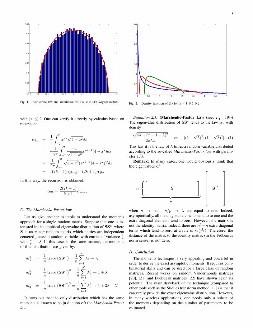
More importantly, the only distribution which has all its oddmoments null and all its even moments equal to the Catalannumbers is known to be the semi-circular law provided by:

f(x) =12π

√4− x2,

3

−2.5 −2 −1.5 −1 −0.5 0 0.5 1 1.5 2 2.50

0.05

0.1

0.15

0.2

0.25

0.3

0.35

Fig. 1. Semicircle law and simulation for a 512× 512 Wigner matrix.

with |x| ≤ 2. One can verify it directly by calculus based onrecursion:

α2k =1π

∫ 2

−2

x2k√

4− x2dx

= − 12π

∫ 2

−2

−x√4− x2

x2k−1(4− x2)dx

=12π

∫ 2

−2

√4− x2(x2k−1(4− x2))′dx

= 4(2k − 1)α2k−2 − (2k + 1)α2k.

In this way, the recursion is obtained:

α2k =2(2k − 1)

k + 1α2k−2.

C. The Marchenko-Pastur law

Let us give another example to understand the momentsapproach for a single random matrix. Suppose that one is in-terested in the empirical eigenvalue distribution of SSH whereS is an n × p random matrix which entries are independentcentered gaussian random variables with entries of variance 1

nwith n

p → λ. In this case, in the same manner, the momentsof this distribution are given by:

mn1 =

1n

trace(SSH

)=

1n

n∑i=1

λi → λ

mn2 =

1n

trace(SSH

)2=

1n

N∑i=1

λ2i → 1 + λ

mn3 =

1n

trace(SSH

)3=

1n

n∑i=1

λ3i → 1 + 3λ + λ2

It turns out that the only distribution which has the samemoments is known to be (a dilation of) the Marchenko-Pasturlaw.

0 0.5 1 1.5 2 2.5 3 3.5 40

0.5

1

1.5

2

2.5

3

3.5

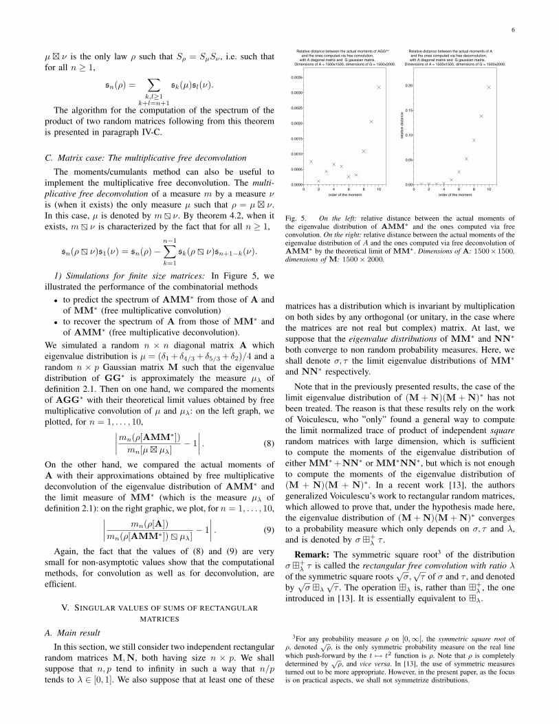
Fig. 2. Density function of (1) for λ = 1, 0.5, 0.2.

Definition 2.1: (Marchenko-Pastur Law (see, e.g. [19]))The eigenvalue distribution of SS∗ tends to the law µλ withdensity√

4λ− (x− 1− λ)2

2πλxon [(1−

√λ)2, (1 +

√λ)2]. (1)

This law it is the law of λ times a random variable distributedaccording to the so-called Marchenko-Pastur law with param-eter 1/λ.

Remark: In many cases, one would obviously think thatthe eigenvalues of

n

S

︸ ︷︷ ︸

p

SH

when n → ∞, n/p → λ are equal to one. Indeed,asymptotically, all the diagonal elements tend to to one and theextra-diagonal elements tend to zero. However, the matrix isnot the identity matrix. Indeed, there are n2−n extra-diagonalterms which tend to zero at a rate of O( 1

n2 ). Therefore, thedistance of the matrix to the identity matrix (in the Frobeniusnorm sense) is not zero.

D. Conclusion

The moments technique is very appealing and powerful inorder to derive the exact asymptotic moments. It requires com-binatorial skills and can be used for a large class of randommatrices. Recent works on random Vandermonde matrices[20], [21] and Euclidean matrices [22] have shown again itspotential. The main drawback of the technique (compared toother tools such as the Stieljes transform method [11]) is that itcan rarely provide the exact eigenvalue distribution. However,in many wireless applications, one needs only a subset ofthe moments depending on the number of parameters to beestimated.

4

III. SUM OF TWO RANDOM MATRICES

A. Scalar case: X + Y

Let us consider two independent random variables X, Yand suppose that we know the distribution of X + Y andY and would like to infer on the distribution of X . Thedistribution of X + Y is the convolution of the distributionof X with the distribution of Y . However, the expression isnot straightforward to obtain. Another way of computing thespectrum is to form the moment generating functions

MX(s) = E(esX), MX+Y (s) = E(es(X+Y )).

It is then immediate to see that

MX(s) = MX+Y (s)/MY (s).

The distribution of X can be recovered from MX(s).This task is however not always easy to perform as theinversion formula does not provide an explicit expression. Itis rather advantageous to express the independence in termsof moments of the distributions or even cumulants. We denoteby Ck the cumulant of order k:

Ck(X) =∂n

∂tn |t=0log

(E

(etX

)).

They behave additively with respect to the convolution, i.e, forall k ≥ 0,

Ck(X + Y ) = Ck(X) + Ck(Y ).

Moments and cumulants of a random variable can easily bededuce from each other by the formula

∀n ≥ 1,mn(X) =n∑

p=1

∑k1≥1,...,kp≥1k1+···+kp=n

Ck1(X) · · ·Ckp(X)

(recall that the moments of a random variable X are thenumbers mn(X) = E(Xn), n ≥ 1).

Thus the derivation of the law of X from the laws of X+Yand Y can be done by computing the cumulants of X by theformula Ck(X) = Ck(X + Y ) − Ck(X) and then deducingthe moments of X from its cumulants.

B. Matrix case: additive free convolution �

1) Definition: It is has been proved by Voiculescu [12]that for An,Bn free2 large n by n Hermitian (or symmetric)random matrices (both of them having i.i.d entries, or one ofthem having a distribution which is invariant under conjugationby any orthogonal matrix), if the eigenvalue distributions ofAn,Bn converge as n tends to infinity to some probabilitymeasures µ, ν, then the eigenvalue distribution of An + Bn

converges to a probability measure which depends only onµ, ν, which is called the additive free convolution of µ and ν,and which will be denoted by µ � ν.

2The concept of freeness is different from independence.

2) Computation of µ � ν by the moment/cumulants ap-proach: Let us consider a probability measure ρ on the realline, which has moments of all orders. We shall denote itsmoments by mn(ρ) :=

∫tndρ(t), n ≥ 1. (Note that in the

case where ρ is the eigenvalue distribution of a d× d matrixA, these moments can easily be computed by the formula:mn(ρ) = 1

d Tr (An)). We shall associate to ρ another se-quence of real numbers, (Kn(ρ))n≥1, called its free cumulants.The sequences (mn(ρ)) and (Kn(ρ)) can be deduced one fromeach other by the fact that the formal power series

Kρ(z) =∑n≥1

Kn(ρ)zn and Mρ(z) =∑n≥1

mn(ρ)zn (2)

are linked by the relation

Kρ(z(Mρ(z) + 1)) = Mρ(z). (3)

Equivalently, for all n ≥ 1, the sequences (m0(ρ), . . . ,mn(ρ))and (K1(ρ), . . . ,Kn(ρ)) can be deduced one from each othervia the relations

m0(ρ) = 1

mn(ρ) = Kn(ρ) +n−1∑k=1

Kk(ρ)∑

l1,...,lk≥0l1+···+lk=n−k

ml1(ρ) · · ·mlk(ρ)

for all n ≥ 1.

Example 3.1: As an example, it is known (e.g. [19]) that thelaw µλ of definition 2.1 has free cumulants Kn(µλ) = λn−1

for all n ≥ 1.The additive free convolution can be computed easily with

the free cumulants via the following characterization [23]:Theorem 3.2: For µ, ν compactly supported, µ � ν is the

only law ρ such that for all n ≥ 1,

Kn(ρ) = Kn(µ) + Kn(ν).3) Simulations for finite size matrices: In Figure 3, we plot,

for k = 1, . . . , 25, the quantity∣∣∣∣mk(ρ[A + MM∗])mk(ν � µλ)

− 1∣∣∣∣ (4)

for A a diagonal random matrix with independent diagonalentries distributed according to ν = (δ0 + δ1)/2 and M agaussian n × p matrix as in definition 2.1. ρ[X] denotes theeigenvalue distribution of the matrix X. The dimensions of Aare 1500× 1500, those of M are 1500× 2000. Interestingly,the values of (4) provide a good match, which shows that themoments/free cumulants approach is a good way to computethe spectrum of sums of free random matrices.

C. Matrix case: additive free deconvolution �

1) Computation of �: The moments/cumulants method canalso be useful to implement the free additive deconvolution.The free additive deconvolution of a measure ρ by a measureν is (when it exists) the only measure µ such that ρ = µ � ν.In this case, µ is denoted by ρ � ν. By Theorem 3.2, when itexists, ρ � ν is characterized by the fact that for all n ≥ 1,Kn(m � ν) = Kn(ρ) − Kn(ν). This operation is very usefulin denoising applications [2], [3]

5

0 5 10 15 20 25

0.00

0.01

0.02

0.03

0.04

0.05

0.06

0.07

0.08

Relative distance between empirical and theoretical moments of A+GG^*, with A diagonal matrix with Bernouilli independent entries and G gaussian matrix. Dimensions of A = 1500 by 1500, dimensions of G = 1500 by 2000.

order of the moment

rela

tive d

ista

nce

Fig. 3. Relative distance between empirical and theoretical moments of A+MM∗, with A diagonal 1500 by 1500 matrix with Bernouilli independentdiagonal entries and M gaussian 150 by 2000 matrix.

0 2 4 6 8 10 12 14 16

0.00

0.01

0.02

0.03

0.04

0.05

Relative distance between the actual moments of A and the moments of A computed via deconvolution of A+G, with A diagonal matrix with uniform independent eigenvalues on [1,2] and G symmetric gaussian matrix. Dimension of the matrices = 3000.

order of the moment

rela

tive

dis

tan

ce

Fig. 4. Relative distance between the actual moments of A and the momentsof A computed via deconvolution of A+B, with A diagonal 3000× 3000matrix with uniform independent diagonal entries and B gaussian symmetric3000× 3000 matrix.

2) Simulations for finite size matrices: In Figure 4, we plotfor n = 1, . . . , 15, the following values:∣∣∣∣mn(ρ[(A + B) � B])

mn(ρ[A])− 1

∣∣∣∣ (5)

for A a diagonal random matrix which spectrum is chosenat random (the diagonal entries of B are independent anduniformly distributed on [0, 1]) and B a Gaussian symmetricmatrix. The dimension of the matrices is 3000. Again, the factthat the values of (5) match even in the non-asymptotic caseshows that the computational method, for deconvolution, iseffecient.

IV. PRODUCT OF TWO RANDOM MATRICES

A. Scalar case: XY

Suppose now that we are given two classical randomvariables X, Y , assumed to be independent. How do we

find the distribution of X when only the distributions ofXY and Y are given? The solution is quite straightfor-ward since E((XY )k) = E(Xk)E(Y k), so that E(Xk) =E((XY )k)/E(Y k). Hence, using the moments approach, onehas a simple algorithm to compute all the moments of thedistribution. The case of matrices is rather involved and isexplained in the following.

B. Matrix case: multiplicative free convolution �

1) Definition: It is has been proved by Voiculescu [12] thatfor An,Bn free large n×n positive Hermitian (or symmetric)random matrices (both of them having i.i.d entries, or one ofthem having a distribution which is invariant under multiplica-tion by any orthogonal matrix), if the eigenvalue distributionsof An,Bn converge, as n tends to infinity, to some probabilitymeasures µ, ν, then the eigenvalue distribution of AnBn,which is equal to the eigenvalue distribution of A

12 BA

12

converges to a probability measure which depends only onµ, ν. The measure is called the multiplicative free convolutionof µ and ν and will be denoted by µ � ν.

2) Computation of µ � ν by the moment/cumulants ap-proach: Let us consider a probability measure ρ on [0,+∞[,which is not the Dirac mass at zero and which has momentsof all order. We shall denote by

{mn(ρ) :=

∫tndρ(t)

}n≥0

the sequence of its moments. We shall associate to ρ an-other sequence of real numbers, {sn(ρ)}n≥0, which are thecoefficients of what is called its S-transform. The sequences{mn(ρ)} and {sn(ρ)} can be deduced one from each otherby the fact that the formal power series

Sρ(z) =∑n≥1

sn(ρ)zn−1 and Mρ(z) =∑n≥1

mn(ρ)zn (6)

are linked by the relation

Mρ(z)Sρ(Mρ(z)) = z(1 + Mρ(z)). (7)

Equivalently, for all n ≥ 1, the sequences{m1(ρ), . . . ,mn(ρ)} and {s1(ρ), . . . , sn(ρ)} can be deducedone from each other via the relations

m1(ρ)s1(ρ) = 1,

mn(ρ) =∑n+1

k=1 sk(ρ)∑

l1,...,lk≥1l1+···+lk=n+1

ml1(ρ) · · ·mlk(ρ).

Remark Note that these equations allow computationswhich run faster than the ones already implemented (e.g.[10]), because those ones are based on the computation of thecoefficients sn via non crossing partitions and the Krewerascomplement, which use more machine time.

Example 4.1: As an example, it can be shown that forthe law µλ of definition 2.1, that for all n ≥ 1, sn(µλ) =(−λ)n−1.

The multiplicative free convolution can be computed easilywith the free cumulants via the following characterization [23].

Theorem 4.2: For µ, ν compactly supported probabilitymeasures on [0,∞[, non of them being the Dirac mass at zero,

6

µ � ν is the only law ρ such that Sρ = SµSν , i.e. such thatfor all n ≥ 1,

sn(ρ) =∑

k,l≥1k+l=n+1

sk(µ)sl(ν).

The algorithm for the computation of the spectrum of theproduct of two random matrices following from this theoremis presented in paragraph IV-C.

C. Matrix case: The multiplicative free deconvolution

The moments/cumulants method can also be useful toimplement the multiplicative free deconvolution. The multi-plicative free deconvolution of a measure m by a measure νis (when it exists) the only measure µ such that ρ = µ � ν.In this case, µ is denoted by m � ν. By theorem 4.2, when itexists, m � ν is characterized by the fact that for all n ≥ 1,

sn(ρ � ν)s1(ν) = sn(ρ)−n−1∑k=1

sk(ρ � ν)sn+1−k(ν).

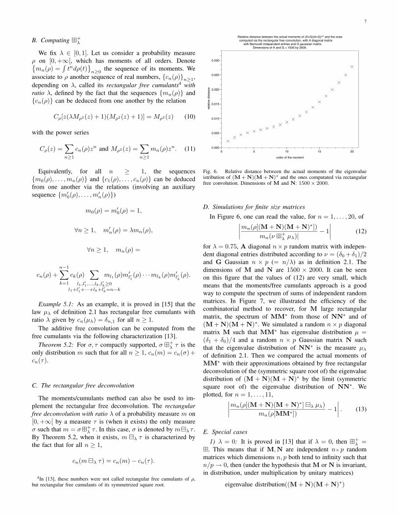
1) Simulations for finite size matrices: In Figure 5, weillustrated the performance of the combinatorial methods• to predict the spectrum of AMM∗ from those of A and

of MM∗ (free multiplicative convolution)• to recover the spectrum of A from those of MM∗ and

of AMM∗ (free multiplicative deconvolution).We simulated a random n × n diagonal matrix A whicheigenvalue distribution is µ = (δ1 + δ4/3 + δ5/3 + δ2)/4 and arandom n × p Gaussian matrix M such that the eigenvaluedistribution of GG∗ is approximately the measure µλ ofdefinition 2.1. Then on one hand, we compared the momentsof AGG∗ with their theoretical limit values obtained by freemultiplicative convolution of µ and µλ: on the left graph, weplotted, for n = 1, . . . , 10,∣∣∣∣mn(ρ[AMM∗])

mn[µ � µλ]− 1

∣∣∣∣ . (8)

On the other hand, we compared the actual moments ofA with their approximations obtained by free multiplicativedeconvolution of the eigenvalue distribution of AMM∗ andthe limit measure of MM∗ (which is the measure µλ ofdefinition 2.1): on the right graphic, we plot, for n = 1, . . . , 10,∣∣∣∣ mn(ρ[A])

mn(ρ[AMM∗]) � µλ]− 1

∣∣∣∣ . (9)

Again, the fact that the values of (8) and (9) are verysmall for non-asymptotic values show that the computationalmethods, for convolution as well as for deconvolution, areefficient.

V. SINGULAR VALUES OF SUMS OF RECTANGULARMATRICES

A. Main result

In this section, we still consider two independent rectangularrandom matrices M,N, both having size n × p. We shallsuppose that n, p tend to infinity in such a way that n/ptends to λ ∈ [0, 1]. We also suppose that at least one of these

0 2 4 6 8 100.0000

0.0005

0.0010

0.0015

0.0020

0.0025

0.0030

0.0035

Relative distance between the actual moments of AGG^* and the ones computed via free convolution, with A diagonal matrix and G gaussian matrix. Dimensions of A = 1500x1500, dimensions of G = 1500x2000.

order of the moment0 2 4 6 8 10

0.00

0.05

0.10

0.15

0.20

Relative distance between the actual moments of A and the ones computed via free deconvolution, with A diagonal matrix and G gaussian matrix. Dimensions of A = 1500x1500, dimensions of G = 1500x2000.

order of the moment

rela

tive

dist

ance

Fig. 5. On the left: relative distance between the actual moments ofthe eigenvalue distribution of AMM∗ and the ones computed via freeconvolution. On the right: relative distance between the actual moments of theeigenvalue distribution of A and the ones computed via free deconvolution ofAMM∗ by the theoretical limit of MM∗. Dimensions of A: 1500×1500,dimensions of M: 1500× 2000.

matrices has a distribution which is invariant by multiplicationon both sides by any orthogonal (or unitary, in the case wherethe matrices are not real but complex) matrix. At last, wesuppose that the eigenvalue distributions of MM∗ and NN∗

both converge to non random probability measures. Here, weshall denote σ, τ the limit eigenvalue distributions of MM∗

and NN∗ respectively.

Note that in the previously presented results, the case of thelimit eigenvalue distribution of (M + N)(M + N)∗ has notbeen treated. The reason is that these results rely on the workof Voiculescu, who ”only” found a general way to computethe limit normalized trace of product of independent squarerandom matrices with large dimension, which is sufficientto compute the moments of the eigenvalue distribution ofeither MM∗+NN∗ or MM∗NN∗, but which is not enoughto compute the moments of the eigenvalue distribution of(M + N)(M + N)∗. In a recent work [13], the authorsgeneralized Voiculescu’s work to rectangular random matrices,which allowed to prove that, under the hypothesis made here,the eigenvalue distribution of (M + N)(M + N)∗ convergesto a probability measure which only depends on σ, τ and λ,and is denoted by σ �+

λ τ .

Remark: The symmetric square root3 of the distributionσ �+

λ τ is called the rectangular free convolution with ratio λof the symmetric square roots

√σ,√

τ of σ and τ , and denotedby√

σ �λ√

τ . The operation �λ is, rather than �+λ , the one

introduced in [13]. It is essentially equivalent to �λ.

3For any probability measure ρ on [0,∞[, the symmetric square root ofρ, denoted

√ρ, is the only symmetric probability measure on the real line

which push-forward by the t 7→ t2 function is ρ. Note that ρ is completelydetermined by

√ρ, and vice versa. In [13], the use of symmetric measures

turned out to be more appropriate. However, in the present paper, as the focusis on practical aspects, we shall not symmetrize distributions.

7

B. Computing �+λ

We fix λ ∈ [0, 1]. Let us consider a probability measureρ on [0,+∞[, which has moments of all orders. Denote{mn(ρ) =

∫tndρ(t)

}n≥0

the sequence of its moments. Weassociate to ρ another sequence of real numbers, {cn(ρ)}n≥1,depending on λ, called its rectangular free cumulants4 withratio λ, defined by the fact that the sequences {mn(ρ)} and{cn(ρ)} can be deduced from one another by the relation

Cρ[z(λMρ2(z) + 1)(Mρ2(z) + 1)] = Mρ2(z) (10)

with the power series

Cρ(z) =∑n≥1

cn(ρ)zn and Mρ2(z) =∑n≥1

mn(ρ)zn. (11)

Equivalently, for all n ≥ 1, the sequences{m0(ρ), . . . ,mn(ρ)} and {c1(ρ), . . . , cn(ρ)} can be deducedfrom one another via the relations (involving an auxiliarysequence {m′

0(ρ), . . . ,m′n(ρ)})

m0(ρ) = m′0(ρ) = 1,

∀n ≥ 1, m′n(ρ) = λmn(ρ),

∀n ≥ 1, mn(ρ) =

cn(ρ) +n−1∑k=1

ck(ρ)∑

l1,l′1,...,lk,l′k≥0

l1+l′1+···+lk+l′k=n−k

ml1(ρ)m′l′1

(ρ) · · ·mlk(ρ)m′l′k

(ρ).

Example 5.1: As an example, it is proved in [15] that thelaw µλ of definition 2.1 has rectangular free cumulants withratio λ given by cn(µλ) = δn,1 for all n ≥ 1.

The additive free convolution can be computed from thefree cumulants via the following characterization [13].

Theorem 5.2: For σ, τ compactly supported, σ �+λ τ is the

only distribution m such that for all n ≥ 1, cn(m) = cn(σ)+cn(τ).

C. The rectangular free deconvolution

The moments/cumulants method can also be used to im-plement the rectangular free deconvolution. The rectangularfree deconvolution with ratio λ of a probability measure m on[0,+∞[ by a measure τ is (when it exists) the only measureσ such that m = σ�+

λ τ . In this case, σ is denoted by m�λ τ .By Theorem 5.2, when it exists, m �λ τ is characterized bythe fact that for all n ≥ 1,

cn(m �λ τ) = cn(m)− cn(τ).

4In [13], these numbers were not called rectangular free cumulants of ρ,but rectangular free cumulants of its symmetrized square root.

0 5 10 15 20

0.000

0.005

0.010

0.015

0.020

0.025

0.030

Relative distance between the actual moments of (A+G)(A+G)^* and the ones computed via the rectangular free convolution, with A diagonal matrix with Bernouilli independent entries and G gaussian matrix. Dimensions of A and G = 1500 by 2000.

order of the moment

rela

tive d

ista

nce

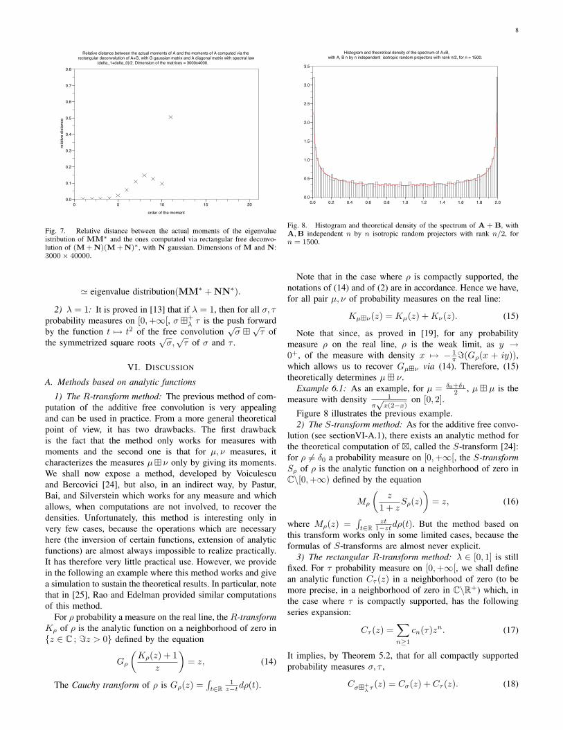
Fig. 6. Relative distance between the actual moments of the eigenvalueistribution of (M + N)(M + N)∗ and the ones computated via rectangularfree convolution. Dimensions of M and N: 1500× 2000.

D. Simulations for finite size matrices

In Figure 6, one can read the value, for n = 1, . . . , 20, of∣∣∣∣mn(ρ[(M + N)(M + N)∗])mn(ν �+

λ µλ)|− 1

∣∣∣∣ (12)

for λ = 0.75, A diagonal n× p random matrix with indepen-dent diagonal entries distributed according to ν = (δ0 + δ1)/2and G Gaussian n × p (= n/λ) as in definition 2.1. Thedimensions of M and N are 1500 × 2000. It can be seenon this figure that the values of (12) are very small, whichmeans that the moments/free cumulants approach is a goodway to compute the spectrum of sums of independent randommatrices. In Figure 7, we illustrated the efficiency of thecombinatorial method to recover, for M large rectangularmatrix, the spectrum of MM∗ from those of NN∗ and of(M + N)(M + N)∗. We simulated a random n× p diagonalmatrix M such that MM∗ has eigenvalue distribution µ =(δ1 + δ0)/4 and a random n × p Gaussian matrix N suchthat the eigenvalue distribution of NN∗ is the measure µλ

of definition 2.1. Then we compared the actual moments ofMM∗ with their approximations obtained by free rectangulardeconvolution of the (symmetric square root of) the eigenvaluedistribution of (M + N)(M + N)∗ by the limit (symmetricsquare root of) the eigenvalue distribution of NN∗. Weplotted, for n = 1, . . . , 11,∣∣∣∣mn(ρ[(M + N)(M + N)∗] �λ µλ)

mn(ρ[MM∗])− 1

∣∣∣∣ . (13)

E. Special cases

1) λ = 0: It is proved in [13] that if λ = 0, then �+λ =

�. This means that if M,N are independent n×p randommatrices which dimensions n, p both tend to infinity such thatn/p → 0, then (under the hypothesis that M or N is invariant,in distribution, under multiplication by unitary matrices)

eigenvalue distribution((M + N)(M + N)∗)

8

0 5 10 15 20

0.0

0.1

0.2

0.3

0.4

0.5

0.6

0.7

0.8

Relative distance between the actual moments of A and the moments of A computed via the rectangular deconvolution of A+G, with G gaussian matrix and A diagonal matrix with spectral law (delta_1+delta_0)/2. Dimension of the matrices = 3000x4000.

order of the moment

rela

tive

dis

tan

ce

Fig. 7. Relative distance between the actual moments of the eigenvalueistribution of MM∗ and the ones computated via rectangular free deconvo-lution of (M + N)(M + N)∗, with N gaussian. Dimensions of M and N:3000× 40000.

' eigenvalue distribution(MM∗ + NN∗).

2) λ = 1: It is proved in [13] that if λ = 1, then for all σ, τprobability measures on [0,+∞[, σ �+

λ τ is the push forwardby the function t 7→ t2 of the free convolution

√σ �

√τ of

the symmetrized square roots√

σ,√

τ of σ and τ .

VI. DISCUSSION

A. Methods based on analytic functions

1) The R-transform method: The previous method of com-putation of the additive free convolution is very appealingand can be used in practice. From a more general theoreticalpoint of view, it has two drawbacks. The first drawbackis the fact that the method only works for measures withmoments and the second one is that for µ, ν measures, itcharacterizes the measures µ � ν only by giving its moments.We shall now expose a method, developed by Voiculescuand Bercovici [24], but also, in an indirect way, by Pastur,Bai, and Silverstein which works for any measure and whichallows, when computations are not involved, to recover thedensities. Unfortunately, this method is interesting only invery few cases, because the operations which are necessaryhere (the inversion of certain functions, extension of analyticfunctions) are almost always impossible to realize practically.It has therefore very little practical use. However, we providein the following an example where this method works and givea simulation to sustain the theoretical results. In particular, notethat in [25], Rao and Edelman provided similar computationsof this method.

For ρ probability a measure on the real line, the R-transformKρ of ρ is the analytic function on a neighborhood of zero in{z ∈ C ; =z > 0} defined by the equation

Gρ

(Kρ(z) + 1

z

)= z, (14)

The Cauchy transform of ρ is Gρ(z) =∫

t∈R1

z−tdρ(t).

0.0 0.2 0.4 0.6 0.8 1.0 1.2 1.4 1.6 1.8 2.00.0

0.5

1.0

1.5

2.0

2.5

3.0

3.5

Histogram and theoretical density of the spectrum of A+B, with A, B n by n independent isotropic random projectors with rank n/2, for n = 1500.

Fig. 8. Histogram and theoretical density of the spectrum of A + B, withA,B independent n by n isotropic random projectors with rank n/2, forn = 1500.

Note that in the case where ρ is compactly supported, thenotations of (14) and of (2) are in accordance. Hence we have,for all pair µ, ν of probability measures on the real line:

Kµ�ν(z) = Kµ(z) + Kν(z). (15)

Note that since, as proved in [19], for any probabilitymeasure ρ on the real line, ρ is the weak limit, as y →0+, of the measure with density x 7→ − 1

π=(Gρ(x + iy)),which allows us to recover Gµ�ν via (14). Therefore, (15)theoretically determines µ � ν.

Example 6.1: As an example, for µ = δ0+δ12 , µ � µ is the

measure with density 1

π√

x(2−x)on [0, 2].

Figure 8 illustrates the previous example.2) The S-transform method: As for the additive free convo-

lution (see sectionVI-A.1), there exists an analytic method forthe theoretical computation of �, called the S-transform [24]:for ρ 6= δ0 a probability measure on [0,+∞[, the S-transformSρ of ρ is the analytic function on a neighborhood of zero inC\[0,+∞) defined by the equation

Mρ

(z

1 + zSρ(z)

)= z, (16)

where Mρ(z) =∫

t∈Rzt

1−ztdρ(t). But the method based onthis transform works only in some limited cases, because theformulas of S-transforms are almost never explicit.

3) The rectangular R-transform method: λ ∈ [0, 1] is stillfixed. For τ probability measure on [0,+∞[, we shall definean analytic function Cτ (z) in a neighborhood of zero (to bemore precise, in a neighborhood of zero in C\R+) which, inthe case where τ is compactly supported, has the followingseries expansion:

Cτ (z) =∑n≥1

cn(τ)zn. (17)

It implies, by Theorem 5.2, that for all compactly supportedprobability measures σ, τ ,

Cσ�+λ τ (z) = Cσ(z) + Cτ (z). (18)

9

Hence the analytic transform Cρ somehow ”linearizes” thebinary operation �+

λ on the set of probability measures on[0,+∞[. The analytic function Cρ is called the rectangularR-transform5 with ratio λ of ρ.

It happens, as shown below, that for any probability measureρ on [0,+∞[, Cρ can be computed in a direct way, withoutusing the definition of (17).

Let us define Mρ(z) =∫

t∈R+zt

1−ztdρ(t). Then the analyticfunction Cρ is defined in a neighborhood of zero (in C\R+)to be the solution of

Cρ[z(λMρ(z) + 1)(Mρ(z) + 1)] = Mρ(z). (19)

which tends to zero for z → 0.To give a more explicit definition of Cρ, let us define

Hρ(z) = z(λMρ(z) + 1)(Mρ(z) + 1).

Then

Cρ(z) = U

(z

H−1ρ (z)

− 1)

with

U(z) =

{−λ−1+((λ+1)2+4λz)

12

2λ if λ 6= 0,z if λ = 0,

where z 7→ z12 is the analytic version of the square root defined

on C\R− such that 112 = 1 and H−1

ρ is the inverse (in thesense of the composition) of Hρ.

To recover ρ from Cρ, one has to go the inverse way:

H−1ρ (z) =

z

(λCρ(z) + 1)(Cρ(z) + 1)

and

Mρ(z) = U

(Hρ(z)

z− 1

),

from what one can recover ρ, via its Cauchy transform.Note that all this method is working for non compactly

supported probability measures, and that (18) is valid for anypair of symmetric probability measures.

As for � and �, analytic functions give us a new way tocompute the multiplicative free convolution of two symmetricprobability measures τ, σ. However, the operations which arenecessary in this method (the inversion of certain functions,the extension of certain analytic functions) are almost alwaysimpossible to realize in pratice. However, in the followingexample, computations are less involved.

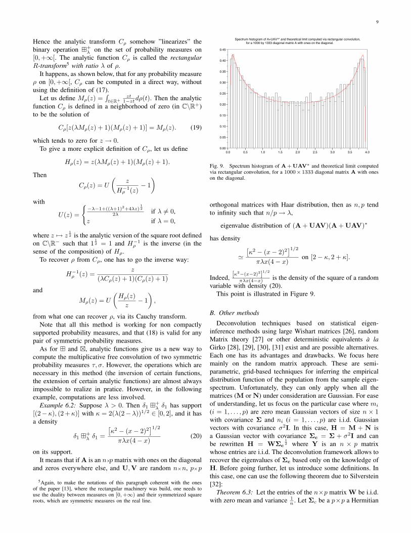
Example 6.2: Suppose λ > 0. Then δ1 �+λ δ1 has support

[(2− κ), (2 + κ)] with κ = 2(λ(2− λ))1/2 ∈ [0, 2], and it hasa density

δ1 �+λ δ1 =

[κ2 − (x− 2)2

]1/2

πλx(4− x)(20)

on its support.It means that if A is an n×p matrix with ones on the diagonal

and zeros everywhere else, and U,V are random n×n, p×p

5Again, to make the notations of this paragraph coherent with the onesof the paper [13], where the rectangular machinery was build, one needs touse the duality between measures on [0, +∞) and their symmetrized squareroots, which are symmetric measures on the real line.

0.0 0.5 1.0 1.5 2.0 2.5 3.0 3.5 4.0

0.00

0.05

0.10

0.15

0.20

0.25

0.30

0.35

0.40

0.45

Spectrum histogram of A+UAV^* and theoretical limit computed via rectangular convolution, for a 1000 by 1333 diagonal matrix A with ones on the diagonal.

Fig. 9. Spectrum histogram of A + UAV∗ and theoretical limit computedvia rectangular convolution, for a 1000× 1333 diagonal matrix A with oneson the diagonal.

orthogonal matrices with Haar distribution, then as n, p tendto infinity such that n/p → λ,

eigenvalue distribution of (A + UAV)(A + UAV)∗

has density

'[κ2 − (x− 2)2

]1/2

πλx(4− x)on [2− κ, 2 + κ].

Indeed, [κ2−(x−2)2]1/2

πλx(4−x) is the density of the square of a randomvariable with density (20).

This point is illustrated in Figure 9.

B. Other methods

Deconvolution techniques based on statistical eigen-inference methods using large Wishart matrices [26], randomMatrix theory [27] or other deterministic equivalents a laGirko [28], [29], [30], [31] exist and are possible alternatives.Each one has its advantages and drawbacks. We focus heremainly on the random matrix approach. These are semi-parametric, grid-based techniques for inferring the empiricaldistribution function of the population from the sample eigen-spectrum. Unfortunately, they can only apply when all thematrices (M or N) under consideration are Gaussian. For easeof understanding, let us focus on the particular case where mi

(i = 1, . . . , p) are zero mean Gaussian vectors of size n × 1with covariance Σ and ni (i = 1, . . . , p) are i.i.d. Gaussianvectors with covariance σ2I. In this case, H = M + N isa Gaussian vector with covariance Σc = Σ + σ2I and canbe rewritten H = WΣc

12 where Y is an n × p matrix

whose entries are i.i.d. The deconvolution framework allows torecover the eigenvalues of Σc based only on the knowledge ofH. Before going further, let us introduce some definitions. Inthis case, one can use the following theorem due to Silverstein[32]:

Theorem 6.3: Let the entries of the n×p matrix W be i.i.d.with zero mean and variance 1

n . Let Σc be a p×p a Hermitian

10

matrix with an empirical distribution converging almost surelyin distribution to a probability distribution PΣc(x) as p →∞.Then almost surely, the empirical eigenvalue distribution ofthe random matrix:

HH∗ = WΣcW∗

converges weakly, as p, n → ∞ with pn fixed, to the unique

nonrandom distribution function whose Stieltjes transformsatisfies:

− 1GHH∗(z)

= z − p

n

∫ydPΣc(y)

1 + yGHH∗(z).

Let us now explain the deconvolution framework in thisspecific case.• In the first step, one can compute GHH∗(z) =

1n trace(HH∗ − zI)−1 for any z. The algorithm startsby evaluating GHH∗ on a grid of a set of values (zj)

Jn

j=1.The more values are considered (big value of Jn), themore accurate the result will be.

• In the second step, dPΣc is approximated by a weightedsum of point masses:

dPΣc(y) ∼K∑

k=1

wkδ(tk − y)

where tk, k = 1, ..K is a chosen grid of points and wk ≥0 are such that

∑Kk=1 wk = 1. The approximation turns

the problem of optimization over measures into a searchfor a vector of weights {w1, ...wK} in RK

+ .• In this case, we have that:∫

ydPΣc(y)1 + yGHH∗(z)

∼K∑

k=1

wktk

1 + tkGHH∗(z)

Hence the whole problem becomes an optimization prob-lem: minimize

maxj=1,..Jn

max (| <(ej) |, | =(ej) |)

subject to∑K

k=1 wk = 1 and wk ≥ 0 for all k, where

ej =1

1n trace(HH∗ − zjI)−1

+ zj

− p

n

∑k=1

Kwktk

1 + tk1n trace(HH∗ − zjI)−1

.

The optimization procedure is a Linear program which canbe solved numerically. Note that although there are severalsources of errors due to the approximations of the integrals andthe replacement of asymptotic quantities by non-asymptoticones, [27] shows remarkably that the solution is consistent (interms of size of available data and grid points on which toevaluate the functions).

The assumptions for the cumulants approach are a bit moregeneral, because we do not suppose the random matrices weconsider to be Gaussian. But the main difference lies in theway we approximate the distribution PΣc : we give moments,whereas here, PΣc is approximated by a linear combinationof Dirac masses.

VII. ENTROPY RATE AND SPECTRUM

In wireless intelligent random networks, devices are au-tonomous and should take decisions based on their sensingcapabilities. Of particularly interest are information measuressuch as capacity, signal to noise ratio, estimation of powers oreven topology identification. Information measures are usuallyrelated to the spectrum (eigenvalues) of the matrices modellingthe underlying network and not on the specific structure(eigenvectors). This entails many simplifications that makefree deconvolution a very appealing framework for the designof these networks. In the following, we provide only oneexample of the applications of free deconvolution to wirelesscommunications. Others can be found in [9].

The entropy rate [33]of a stationnary Gaussian stochasticprocess, upon which many information theoretic performancemeasures are based, can be expressed as:

H = log(πe) +12π

∫ π

−π

log(S(f))df,

where S is the spectral density of the process. Hence, if oneknows the autocorrelation of the process, one has thereforea full characterization of the information contained in theprocess. Moreover, as side result, one can also show that theentropy rate is also related to the minimum mean squarederror of the best estimator of the process given the infinitepast [34], [35]. This remarkable result is of main interestfor wireless communications as one can deduce one quantityfrom the other, especially as many receivers incorporate anMMSE (Minimum Mean Square Error) component. Theseresults show the central importance of the autocorrelationfunction for Gaussian processes. In the discrete case whenconsidering a random Gaussian vector x of size n, the entropyrate per dimension (or differential entropy) is given by:

H = log(πe) +1n

log det(R)

= log(πe) +1n

n∑i=1

log(λi), (21)

where R = E(xix∗i ) and λi the associated eigenvalues.The covariance matrix (and more precisely its eigenvalues)carries therefore all the information of Gaussian networks.The Gaussianity of these networks is due to the fact that thenoise, the channel and the signaling are very often Gaussian.Hence, in order to get a reliable estimate of the rate (and inextension of the capacity which is the difference between twodifferential entropies), one needs to compute the eigenvaluesof the covariance matrix. For a number of observations p ofthe vector xi, i = 1, ..., p, the covariance matrix R is usuallyestimated by:

R =1p

p∑i=1

xix∗i (22)

= R12 SS∗R

12 (23)

Here, S = [s1, .., sp] is an n × p i.i.d zero mean Gaussianvector of variance 1

p . In many cases, the number of samples pis of the same order as n. This is mainly due to the fact that

11

the network is highly mobile and the statistics are consideredto be the same within a number p of samples, which restrictsthe use of classical asymptotic signal processing techniques.Therefore, information retrieval must be performed within awindow of limited samples. Example (23) is unfortunatelyrarely encountered in practice in wireless communications.The signal of interest si is usually distorted by a medium,given by mi = f(si) where f is any function. Moreover,the received signal yi is altered by some additive noiseni (not necessarily Gaussian) but in many respect unitarilyinvariant (due to the fact that all the dimensions have thesame importance). In this case, the model is known as theInformation plus Noise model:

yi = mi + ni,

which can be rewritten in the following matrix form bystacking all the observations:

Y = M + N. (24)

We have therefore a signal Y = M + N, with M,Nindependent n × p (n, p >> 1, n/p ' λ) random matrices,M = R

12 S, with S having i.i.d. N(0, 1) entries, and N (the

noise) has i.i.d. N(0, σ) entries. σ is known and supposed tobe measured by the device. From (21), the entropy rate H isgiven by:

H = log(πe) +1n

n∑i=1

log(λi),

where the λi’s are the eigenvalues of R. Hence H can becomputed with the previous method, since H = log(πe) +∫

log(x)dµR(x), where µR denotes the eigenvalue distribu-tion of R. Indeed, µR is given by the formula:

µR = (µ 1p YY∗ �λ µ 1

p NN∗) � µ 1p SS∗ ,

where the eigenvalues distributions µ 1p NN∗ , µ 1

p SS∗ are known,by definition 2.1, to be the Marchenko-Pastur distribution(rescaled by the factor σ in the case of µ 1

p NN∗ ). Usinga polynomial approximation of the logarithm (because µR

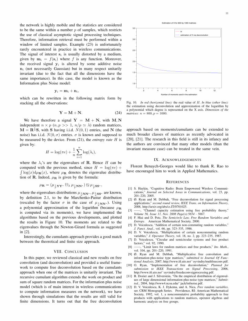
is computed via its moments), we have implemented thealgorithms based on the previous developments, and plottedthe results in Figure 10. The moments are related to theeigenvalues through the Newton-Girard formula as suggestedin [2].

Interestingly, the cumulants approach provides a good matchbetween the theoretical and finite size approach.

VIII. CONCLUSION

In this paper, we reviewed classical and new results on freeconvolution (and deconvolution) and provided a useful frame-work to compute free deconvolution based on the cumulantsapproach when one of the matrices is unitarily invariant. Therecursive cumulant algorithm extends the work on product andsum of square random matrices. For the information plus noisemodel (which is of main interest in wireless communicationsto compute information measures on the network), we haveshown through simulations that the results are still valid forfinite dimensions. It turns out that the free deconvolution

2 4 6 8 10 12

1.0

1.5

2.0

2.5

3.0

3.5

Estimation of H for 800 by 1000 matrices

Number of moments used in the estimation

H

estimation of H via deconvolution

Fig. 10. In red (horizontal line): the real value of H . In blue (other line):the estimation using deconvolution and approximation of the logarithm bya polynomial which degree is represented on the X axis. Dimension of thematrices: n = 800, p = 1000.

approach based on moments/cumulants can be extended tomuch broader classes of matrices as recently advocated in[20], [21]. The research in this field is still in its infancy andthe authors are convinced that many other models (than theinvariant measure case) can be treated in the same vein.

IX. ACKNOWLEDGEMENTS

Florent Benaych-Georges would like to thank R. Rao tohave encouraged him to work in Applied Mathematics.

REFERENCES

[1] S. Haykin, “Cognitive Radio: Brain Empowered Wireless Communi-cations,” Journal on Selected Areas in Communications, vol. 23, pp.201–220, 2005.

[2] Ø. Ryan and M. Debbah, “Free deconvolution for signal processingapplications,” second round review, IEEE Trans. on Information Theory,2008, http://arxiv.org/abs/cs.IT/0701025.

[3] ——, “Channel capacity estimation using free probability theory,”Volume 56, Issue 11, Nov. 2008 Page(s):5654 - 5667.

[4] F. Hiai and D. Petz, The Semicircle Law, Free Random Variables andEntropy. American Mathematical Society, 2000.

[5] D. Voiculescu, “Addition of certain non-commuting random variables,”J. Funct. Anal., vol. 66, pp. 323–335, 1986.

[6] D. V. Voiculescu, “Multiplication of certain noncommuting randomvariables,” J. Operator Theory, vol. 18, no. 2, pp. 223–235, 1987.

[7] D. Voiculescu, “Circular and semicircular systems and free productfactors,” vol. 92, 1990.

[8] ——, “Limit laws for random matrices and free products,” Inv. Math.,vol. 104, pp. 201–220, 1991.

[9] Ø. Ryan and M. Debbah, “Multiplicative free convolution andinformation-plus-noise type matrices,” submitted to Journal Of Func-tional Analysis, 2007, http://www.ifi.uio.no/˜oyvindry/multfreeconv.pdf.

[10] O. Ryan, “Implementation of free deconvolution,” Planned forsubmission to IEEE Transactions on Signal Processing, 2006,http://www.ifi.uio.no/˜oyvindry/freedeconvsigprocessing.pdf.

[11] B. Dozier and J. Silverstein, “On the empirical distribution of eigenval-ues of large dimensional information-plus-noise type matrices,” Submit-ted., 2004, http://www4.ncsu.edu/˜jack/infnoise.pdf.

[12] D. V. Voiculescu, K. J. Dykema, and A. Nica, Free random variables,ser. CRM Monograph Series. Providence, RI: American MathematicalSociety, 1992, vol. 1, a noncommutative probability approach to freeproducts with applications to random matrices, operator algebras andharmonic analysis on free groups.

12

[13] F. Benaych-Georges, “Rectangular random matrices, related convolu-tion,” To appear in Probability Theory and Related Fields.

[14] S. Belinschi, F. Benaych-Georges, and A. Guionnet, “Regularization byfree additive convolution, square and rectangular cases,” To appear inComplex Analysis and Operator Theory.

[15] F. Benaych-Georges, “Infinitely divisible distributions for rectangularfree convolution: classification and matricial interpretation,” Probab.Theory Related Fields, vol. 139, no. 1-2, pp. 143–189, 2007.

[16] E. Wigner, “On the distribution of roots of certain symmetric matrices,”The Annals of Mathematics, vol. 67, pp. 325–327, 1958.

[17] ——, “Characteristic vectors of bordered matrices with infinite dimen-sions,” The Annals of Mathematics, vol. 62, pp. 458–564, 1955.

[18] Conway and Guy, The Book of Numbers. New York: Copernicus, 1996.[19] F. Hiai and D. Petz, The semicircle law, free random variables and

entropy, ser. Mathematical Surveys and Monographs. Providence, RI:American Mathematical Society, 2000, vol. 77.

[20] Ø. Ryan and M. Debbah, “Random Vandermonde matrices-part I:Fundamental results,” Submitted to IEEE Trans. on Information Theory,2008.

[21] ——, “Random Vandermonde matrices-part II: Applications,” Submittedto IEEE Trans. on Information Theory, 2008.

[22] C. Bordenave, “Eigenvalues of euclidean random matrices,” To appearin Random Structures and Algorithms, ArXiv: math.PR/0606624, 2008.

[23] A. Nica and R. Speicher, Lectures on the combinatorics of free probabil-ity, ser. London Mathematical Society Lecture Note Series. Cambridge:Cambridge University Press, 2006, vol. 335.

[24] H. Bercovici and D. Voiculescu, “Free convolution of measures withunbounded support,” Indiana Univ. Math. J., vol. 42, no. 3, pp. 733–773, 1993.

[25] A. Edelman and N. R. Rao, “The polynomial method for randommatrices,” To appear in Foundations of Computational Mathematics.

[26] N. Rao, J. Mingo, R. Speicher, and A. Edelman,“Statistical eigen-inference from large wishart matrices,”http://front.math.ucdavis.edu/0701.5314, Jan, 2007.

[27] N. E. Karoui, “Spectrum estimation for large dimen-sional covariance matrices using random matrix theory,”http://front.math.ucdavis.edu/0609.5418, Sept, 2006.

[28] V. L. Girko, An Introduction to Statistical Analysis of Random Arrays.The Netherlands, VSP, 1998.

[29] ——, Theory of Stochastic Canonical Equations, Volumes I and II.Kluwer Academic Publishers, 2001.

[30] W. Hachem, P. Loubaton, and J. Najim, “Deterministic equivalents forcertain functionals of large random matrices,” The Annals of AppliedProbability, 2007.

[31] X. Mestre, “Improved estimation of eigenvalues of covariance matricesand their associated subspaces using their sample estimates,” submittedto IEEE Transactions on Information Theory, 2008.

[32] J. Silverstein, “Strong convergence of the empirical distribution ofeigenvalues of large dimensional random matrices,” J. of MultivariateAnalysis, vol. 55, pp. 331–339, 1995.

[33] T. Cover and J. Thomas, Elements of Information Theory. Wiley, 1991.[34] D. Guo, S. Shamai, and S. Verdu, “Mutual Information and Minimum

Mean-Square Error in Gaussian Channels,” IEEE Trans. InformationTheory, vol. 51, pp. 1261–1283, 2005.

[35] D. P. Palomar and S. Verdu, “Gradient of Mutual Information in LinearVector Gaussian Channels,” IEEE Trans. Information Theory, vol. 52,pp. 141–154, 2006.