franz hlawatsch, member, ieee, and werner kozek, … · i i248 ieee transactions on signal...

I

I248 IEEE TRANSACTIONS ON SIGNAL PROCESSING, VOL. 41, NO. 3, MARCH 1993

The Wigner Distribution of a Linear Signal Space Franz Hlawatsch, Member, IEEE, and Werner Kozek, Student Member, IEEE

Abstract-We introduce a time-frequency representation of linear signal spaces which we call the Wigner distribution (WO) ofa linear signal space. Similar to the WD of a signal, the WD of a linear signal space describes the space’s energy distribution over the time-frequency plane.

The WD of a signal space can be defined both in a deterministic and in a stochastic framework, and it can be expressed in a simple way in terms of the space’s projection operator and bases. It is shown to satisfy many interesting properties which are often analogous to corresponding properties of the WD of a signal. The results obtained for some specific signal spaces are found to be intuitively satisfactory.

Further topics discussed are the cross-WD of two signal spaces, a discrete-time WD version, and the extension of the WD definition to arbitrary quadratic signal representations.

I. INTRODUCTION OTH for signal theory in general and for the formu- B lation of modem signal processing algorithms, linear

signal spaces and the associated concepts of orthogonal projections and orthonormal bases [ l ] , [2] are of fundamental importance [ l ] , [3]. This paper proposes a joint time-frequency analysis of linear signal spaces by introducing the Wigner distribution (WD) of a linear signal space [4].

The WD of a space is based, both conceptually and mathematically, on the well-known WD of a signal x(t) PI, ~61:

(1.1) W,(t, f ) is a quadratic time-frequency (TF) signal representation which can be interpreted (with some restrictions due to the uncertainty principle) as a TF distribution of the signal’s energy. (In (1.1) and subsequent equations, r and f denote time and frequency, respectively, and inte- grations go from - 03 to 03 .)

In analogy to the WD of a signal, the WD of a linear signal space characterizes the space’s TF localization in that it describes the distribution of the space’s energy over a joint TF plane. Loosely speaking, the WD of a space X is the WD of a signal (1. l ) , averaged over all elements x(t) E X of the space X ; it thus indicates the overall TF region where the elements x(t) E X take on their energy.

Manuscript received August 14, 1991; revised February 21, 1992. This work was supported in part by the Fonds zur Forderung der wissenschaft- lichen Forschung under Grant P7354-PHY.

The authors are with the Institut fur Nachrichtentechnik und Hochfre- quenztechnik, Technische Universitat Wien, A-1040 Vienna, Austria.

IEEE Log Number 9206035.

The paper is organized as follows. In Section 11, the WD of a space is defined in both a deterministic and a stochastic framework, expressions in terms of the space’s projection operator and bases are given, and the extension of these definitions and expressions to arbitrary quadratic representations is considered. Section I11 shows that the WD of a space satisfies a number of interesting properties, and Section IV discusses the WD’s energetic interpretation. The results obtained for some specific spaces are considered in Section V. Finally, the cross-WD of two spaces and the discrete-time WD are defined and briefly discussed in Section VI.

By way of introduction, we first review some basic facts about linear signal spaces [ l ] , [2]. A linear signal space X is a collection of signals x(t) such that any linear com- bination clxl ( t ) + c2x2 (t) of two elements x1 ( t ) , x2 ( t ) E X is again an element of X. In this paper, we consider spaces X which are subspaces of the space Q2 (R) of square- integrable (finite-energy) signals, i.e., X is a Hilbert space with inner product ( e , .) and norm 11 )I defined as

The orthogonal projecrion s, ( t ) E X of a signal s ( t ) E P2 (Fa) on a space X is

S x ( t ) = ( X S ) ( ~ ) = X ( t , t ’ ) ~ ( t ’ ) dt’ (1.2) s,, where X is the orthogonal projection operator of X and X ( t , t ’ ) denotes its kernel. An alternative expression is

NX

S x ( t ) = ,c, SkXk(t) with Sk = (S, Xk)

where {xk(t)} (k = 1, , N , ) is an orthonormal basis of X and N , (which may be infinite) is the dimension of X. In the following, “projection,” “projection operator,” and “basis” stand for orthogonal projection, orthogonal projection operator, and orthonormal basis, respectively. Both the projection operator X and the basis {xk(t)} characterize the space X, although the basis {xk(t)} is not uniquely defined. The projection operator is idempotent (X2 = X) and self-adjoint (X’ = X where X’ denotes the adjoint of the operator X with kernel X’ ( t , r ’ ) = X * ( t ‘ , t ) ) , and it can be expressed in terms of any basis {xk(t)} of X as

NE

X ( t , t ’ ) = ,.g, Xk(OXk*(t’). (1.3)

1053-587X/93$03.00 0 1993 IEEE

~___ ._ ~

Copyright IEEE 1993

HLAWATSCH A N D KOZEK: W D OF LINEAR SIGNAL SPACE 1249

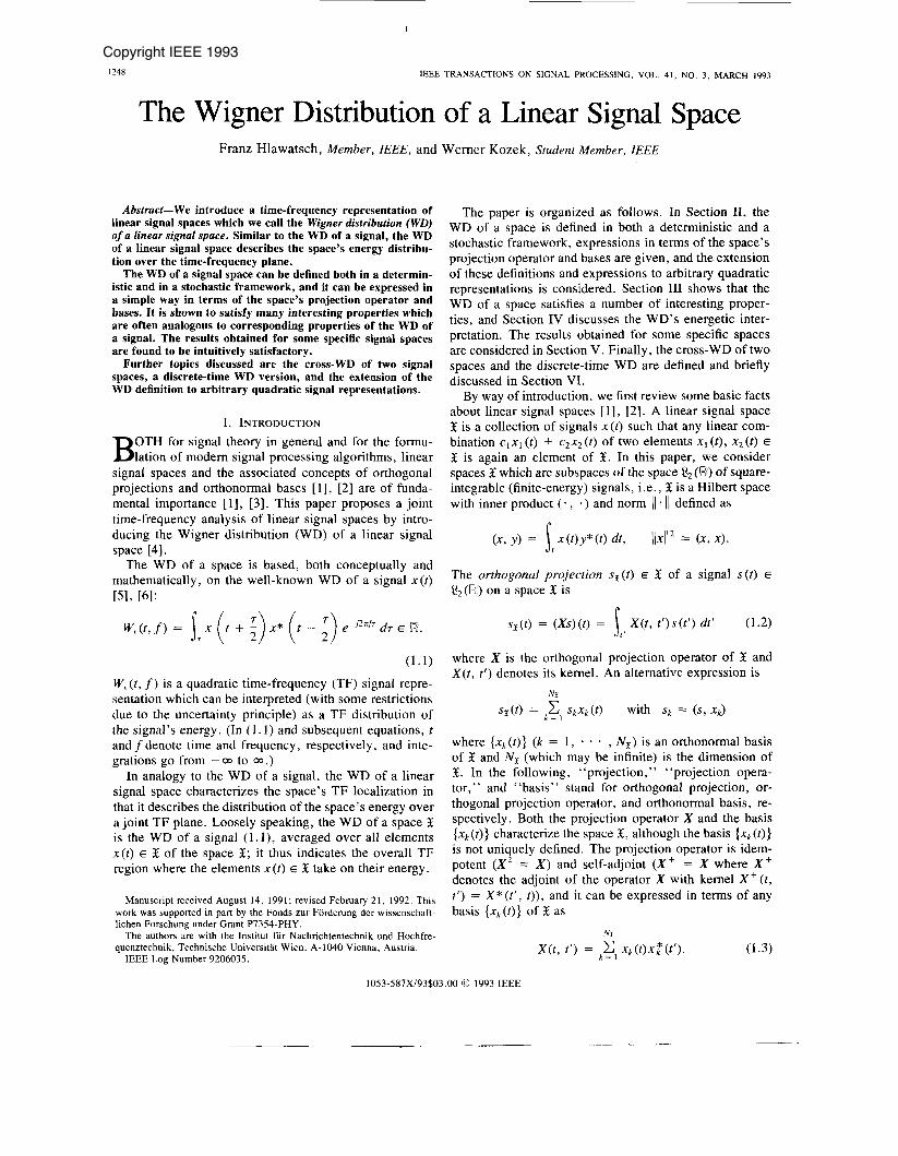
a3 CD c W,,(t,f) = €{W,(t,f)} C W,,,,(t,f) = E{Ww,(t,f)} k=l k=l

Fig. 1. Deterministic and stochastic definitions of W x ( f , f).

11. DEFINITIONS AND EXPRESSIONS Since a signal space X is a collection of individual sig-

nals x ( t ) , it is natural to define the TF energy distribution (WD) of a space X by averaging over the TF energy dis- tributions (WD’s) of all signals x ( t ) E X . We now consider two implementations of this “averaging” which will turn out to yield identical results. The corresponding definitions of the WD of a space are illustrated in Fig. 1.

A . Deterministic Definition Let { lk( t )} ( k = 1, 2, *

mal) basis of P2(R). The projection operator of Q2(R) is

L(t , t ’ ) = C Ik(t)I:(t’) = s(t - t’)

- ) be an arbitrary (orthonor-

ca

(2.1a) k = I

from which it follows with (1.1) that 8

c W r , ( t , f ) 3 1. (2. Ib) k = 1

This shows that the average (sum) of the WD’s of all basis signals Ik(t) covers the entire TF plane in an ideally ho- mogeneous manner. In contrast, the average of the WD’s of the projections l k , ( t ) of all basis signals lk ( t ) on X will be restricted to those regions of the TF plane where the elements x ( t ) E X take on their energy (cf. Fig. 1). We therefore define the WD of the signal space E as

m

W x ( t , f ) e c w k , x ( t , f ). (2.2) k = I

It can be shown that Wx ( t , f ) is independent of the specific (orthonormal) basis { lk( t )} of Q2(!8) used in (2.2).

B. Stochastic Dejinition Let w ( t ) be wide-sense stationary, zero-mean white

noise with normalized power spectral density, such that

the autocorrelation function of w ( t ) is

R,(t, t ’ ) = E { w ( t ) w * ( t ’ ) } = 6 ( t - t ’ ) (2.3a)

where E denotes the expectation operator. Since the WD of the random process w ( t ) is itself random, we consider the expected value E { W,(t , f ) } which is known as the Wiper-Ville spectrum of w ( t ) [7], [8]. Using (2.3a) in (1. l ) , we obtain

E { W , ( t , f ) } = 1. (2.3b)

This shows that the ensemble average (expectation) of the WD of w ( t ) covers the entire TF plane in an ideally ho- mogeneous manner. In contrast, the ensemble average of the WD of the projection w,( t ) of w ( t ) on X will be restricted to those regions of the TF plane where the elements x ( t ) E E take on their energy (cf. Fig. 1). We therefore define the WD of the signal space X as

K&f)S E C W , , ( t , f ) f . (2.4)

It is obvious that the above two definitions are com- pletely analogous. In fact, it is shown in the Appendix that they are strictly equivalent as well. Thus, either the deterministic definition (2.2) or the stochastic definition (2.4) can be used as the basic definition of the WD of a linear signal space X .

C. Expressions in Terms of the Projection Operator Using (2.2) or (2.4), a straightforward derivation (see

the Appendix) shows that the WD of X can be expressed as

where ( X X + ) ( t , t ’ ) denotes the kernel of the composite operator XX + (obtained by cascading the projection operator X of X and its adjoint X’). Since X is self-adjoint and idempotent, there is X X + = X so that (2.5) reduces

I

I250 IEEE TRANSACTIONS ON SIGNAL PROCESSING, VOL. 41, NO. 3 , MARCH 1993

to

Wx(t, f ) = ST X ( t + i, t - 2 ‘) e-J2TfT dr . (2.6)

This simple expression of W, ( t , f ) in terms of the projection operator X is reminiscent of the WD of a signal as expressed by (1.1). We note that (2.6) is the Weyl symbol [9]-[ll] of the projection operator X. Inversion of (2.6) yields

which shows that the projection operator X can be re- covered from the WD W x ( t , f ) and, hence, that W x ( t , f ) provides a complete characterization of the space X .

A “frequency-domain’’ expression of W x ( t , f ) can be derived by first noting that the projection s , ( t ) as given by (1.2) can be expressed in the frequency domain as

where S( f) and Sx (f) are the Fourier transforms of s ( t ) and s, ( t ) , respectively, and

x(f,f’) = s, X ( t , t ’ )e- j2a(f t - f ’ t ’ ) dt dt’ (2.7) t ’

is the “ frequency-domain kernel” (bifrequency function) of the projection operator X. Inserting (2.7) into (2.6) yields

which is analogous to the “time-domain” expression (2.6).

D. Expressions in Terms of a Basis Insertion of (1.3) into (2.6) results in the expression

NX

Wx(t, f ) = ,c1 Y,,(t, f ) (2.8)

where {Xk(t)} ( k = 1, - * , N,) is any (orthonormal) basis of the space X . It is seen that the WD of a space X is simply the sum of the WD’s of all basis signals x,( t ) . We stress that (2.8) is independent of the specific (orthonormal!) basis of X .

Introducing the “basis vector” x_(t) = (xI ( t ) , x 2 ( t ) , .

* , x N X ( t ) ) T , (2.8) can be written as

which is again similar to the WD of a signal as given by (1.1). (The superscripts and + denote transposition and complex conjugate transposition, respectively .)

E. Quadratic Space Representations An important general property of the WD of a signal is

the fact that any other quadratic signal representation can be derived from the WD via some linear transform [12]. It will be shown in Section I11 that an analogous property holds for the WD of a space, i.e., any other quadratic space representation can be derived from the WD of a space via some linear transform. However, we first have to specify what is meant by “quadratic space representation.”

Any quadratic signal representation T,(Q) can be written as [12], [13]

n n

Here, uT(Q; t l , t2) is a kernel function specifying the signal representation T, and e is a parameter vector (e.g., e = ( t , f ) in the WD case). To a given signal representation T@), we define the corresponding space representation Tx@) by straightforward generalization of the WD definition (2.2) or (2.4):

03

TI(@ C Tik,XEL) = E { T w X ( 8 ) } . (2.9)

We can thus define, e.g., the instantaneous power, spectral energy density, energy, temporal and spectral autocorrelation functions, Rihaczek distribution, spectrogram, and ambiguity function [5, part 1111, [14], [15] of a signal space. From (2.9), expressions of TI@) in terms of the projection operator Xor a basis {Xk(t)} are obtained as (cf. (2.6) and (2.8))

k = I

NX

= k = I T,,(8).

By way of example, we consider three “energetic” quadratic signal representations which will be used in Section 111: i) the instantaneous powerp,(t) = (x( t )I2, ii) the spectral energy density P,(f) = ( X ( f ) I 2 (where X ( f ) denotes the Fourier transform of x ( t ) ) , and iii) the energy E, = l ) ~ \ ) ~ . The corresponding space representations are obtained as

NX

Px(t) x ( t , t ) = ,cl IXk(t)I2, NX

Px(f) %<f,.f) = ,?, IXk(f)I2, Ex =

Note the interesting fact that the energy Ex of a space X turns out to equal the space’s dimension N I .

Quite generally, the following statement can be shown: if two quadratic signal representations T, (e) and T: (e’) are related via a linear transform, then the corresponding quadratic space representations T x ( e ) and T;E (e’) are related via the same linear transform. This will be special- ized to the WD in Section 111.

I

HLAWATSCH AND KOZEK: WD OF LINEAR SIGNAL SPACE 1251

111. PROPERTIES

In this section, some properties of the WD of a space (most of which are analogous to properties of the WD of a signal) are stated without proof.

1) Real-valued. The WD of a space is a real-valued function which, however, is not guaranteed to be every- where nonnegative.

2) Time-frequency integral. The integral of W x ( t , f ) over the entire TF plane equals the dimension of X ,

=1;. . , N E ) and { y , ( t ) } ( 1 = 1, * . , ND) as follows:

(WE, W9) = i,S,. X ( t , t’) Y*(t , t ’ ) dt dt’

Nx Ng

= c c K X k ? Y1)12. (3.5)

This can be viewed as a generalization of Moyal’s for- mula [ 5 , part I].

Using (3.5), it can be shown that (W,, W9) is bounded as

k = l I = 1

s, $i WxK f ) dt df = NE.

IIw,112 = 1 j W i ( t , f) dt df = N I .

(3.1) o I (wx, wD> I min { N , , N ~ } ( I a).

3, Norm. The ’quared norm Of W X ( t , f ) the di- The lower bound is attained if and only if the spaces X and ?J are orthogonal, mension of X ,

(W,, Wg) = 0 @ X 19. (3.6) I f The upper bound is attained if and only if one of the spaces

is a subspace of the other: for example, assuming Ng 5 N , we have

This shows that W x ( t , f ) is square-integrable if and only if X has finite dimension.

Combining properties 2 and 3 gives (WE, Wyj) = Ng ?J c x . (3.7) r r r r

which obviously restricts the behavior of the function W x ( t , f ) . Clearly, (3.2) would be satisfied if W x ( t , f ) assumed only values 0 or 1 . While W, (t, f ) does not generally show this specific behavior, computer simulations indicate that in many cases W, ( t , f ) tends to be oscillatory around the heights 0 or 1 (cf. Section V).

4) Finite support. If all signals x ( t ) E X are time limited in an interval [ t , , t2] (or, equivalently, X is a subspace of the space ‘3[tl, t2] of all signals time limited in [ t l , tZ ] ) , then W x ( t , f ) is zero for all t outside [ r l , t2]:

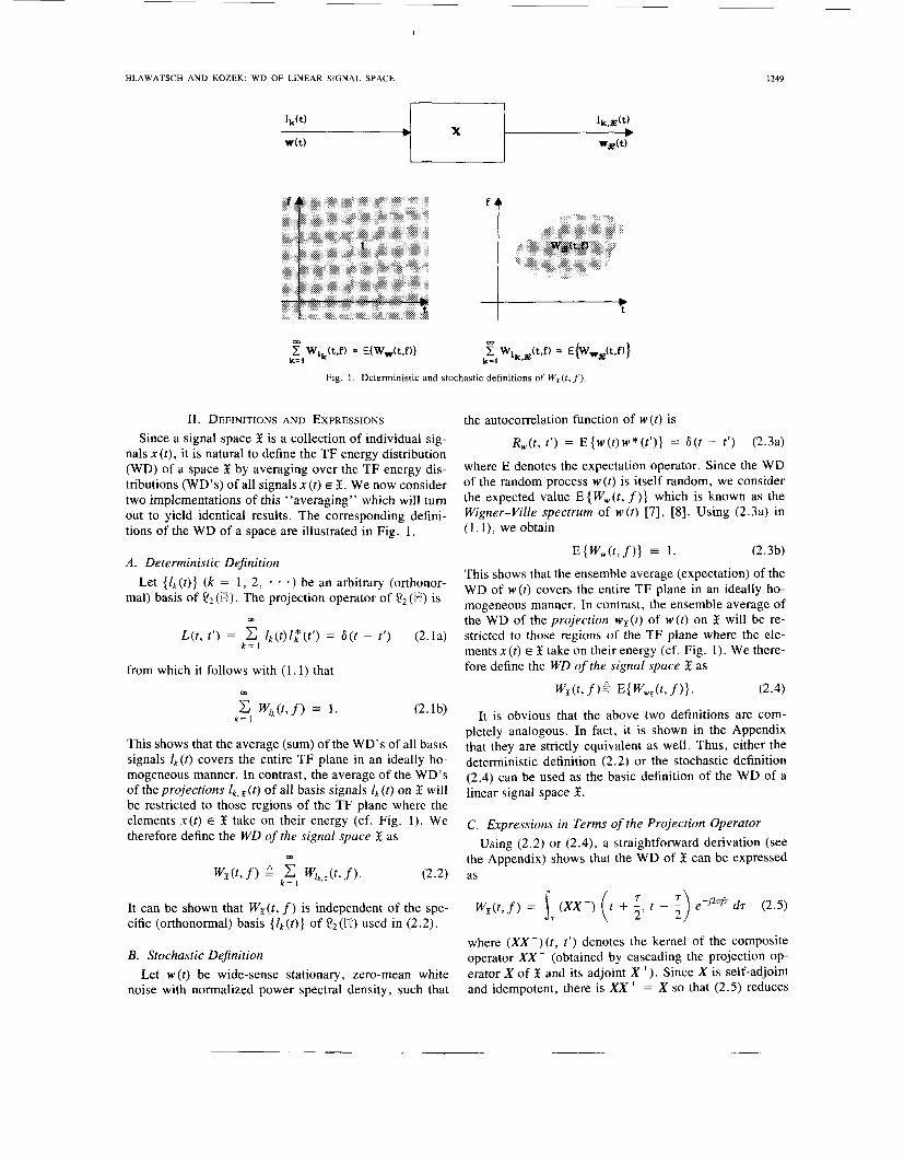
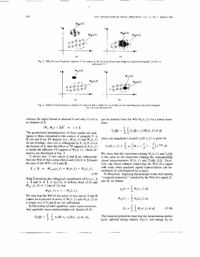
These results lead to important geometrical interpretations. Consider two spaces X and which are time-frequency disjoint in the sense that their WD’s do not overlap (see Fig. 2(a)) and. hence, W,(t, f ) Wg( t , f ) = 0 for all t , f . It follows that (WE, Wg) = 0 and, with (3.6), we conclude that two TF disjoint spaces are orthogonal. (Since exact TF disjointness of two spaces isra very re- strictive condition, we note that this statement still holds in an approximate sense if the spaces are “nearly TF disjoint,” i.e., W , ( t , f ) W g ( t , f ) = 0.)

On the other hand, assume that 9 is a subspace of X . With (3.1), (3.7) can be rewritten as

(3.3)

Similarly, if all signals x ( t > E X are band limited in a frequency band [ f l , f21 (i.e., X is a subspace of the space

f ) is zero for all f outside [ fi , A] :

from which we conclude that if9 is a subspace ofX, then the effective TF support of W, ( t , f ) must be inside the effective TF support of w,ct, f ) . This situation is illustrated in Fig. 2(b).

of a signal s ( t ) and the WD of a signal space X equals the energy of the signal’s projection on X ,

S [ fi 9 fiI Of band limited in [fi 7 f21>, then WX (t , 6) Moyal-type relation 11. The inner product of the WD

X c S[fi9f21 * Wx(t9.f) = 0 f o r f e [ f I , h l . NX

(3.4) (Ws > W,) = Ilsx112 = ,cl I(s, xk)I2 . (3.8)

These properties are analogous to the “finite-support properties7~ satisfied by the WD of a signal [5, part

of two signal spaces X and 9,

This can again be considered a generalization of Moyal’s

as 5) Moyal-type relation 1. The inner product of the WD’s fofmula. It follows from (3.8) that ( Ws, is bounded

0 5 (W?, Wx) 5 11s112.

The lower bound is attained if and only if the signal s ( t ) is orthogonal to the space X ,

can be expressed in terms of the spaces’ projection oper- ( k ators X and Y or in terms of the spaces’ bases { x k (t) (Ws, W,) = 0 e s I X

I252 IEEE TRANSACTIONS ON SIGNAL PROCESSING, VOL. 41. NO. 3. MARCH 1993

w (t f ) ‘t ‘t 7 ’ W,(t,f)

(a) (b)

Fig. 2. Effective time-frequency supports of two spaces X , 9: (a) X and 9 are time-frequency disjointiorthogonal; (b) ’1, is a subspace of X .

W,(t , f ) ‘T f t i I

W,(t , f )

w,c t , f )

/

(a) (b)

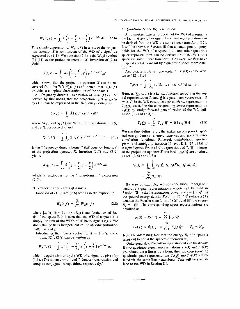
Fig. 3 . Effective time-frequency supports of a space X and a signal s ( t ) : (a) X and s ( r ) are time-frequency disjoint/orthogonal; (b) ~ ( f ) is an element of X .

whereas the upper bound is attained if and only if s ( t ) is can be derived from the WD W x ( t , f) via a linear trans- an element of X , form,

(Ws, WE) = llS1l2 @ s E X . The geometrical interpretations of these results are analogous to those discussed in the context of property 5 : i) If s ( t ) and X are TF disjoint (i.e., W,(t, f) and W x ( t , f) do not overlap), then s ( t ) is orthogonal to X ; ii) if s ( t ) is an element of X , then the effective TF support of W, ( t , f) is inside the effective T F support of W x ( t , f ) . These sit- uations are illustrated in Fig. 3 .

7) Direct sum. If two spaces X and ‘i)) are orthogonal, then the WD of their union (direct sum [2]) X 8 YJ equals the sum of the WD’s of X and YJ,

X 1 2 ) * W x e y ) ( f , f ) = W x ( t , f ) + W&f).

(3.9) With x denoting the orthogonal complement of X (i.e., X I x and X 8 % = Q2 (b)), it follows from (3.9) and WP,( ) ( t , f ) 3 1 (see (5.1)) that

wxct, f , = 1 - W x ( t , f ) .

Tx(8) = s, jtL“ 1, f ) WE@, f > dt df,

where the transform’s kernel L@; t , f ) is given by

We stress that this transform relating W x ( t , f ) and Tx(B) is the same as the transform relating the corresponding signal representations W, ( t , f) and T, (e) [ 121. There- fore, any linear relation connecting the WD of a signal with some other quadratic signal representation can immediately be reformulated for a space.

9) Marginals. Applying this principle to the well-known “marginal properties” satisfied by the WD of a signal [5, part I], we obtain

We note that the WD of the union of two spaces X and ’f)

a simple way if X and cannot be expressed in terms of W E ( [ , f ) and

Any quadratic space representation (cf. Section 11-E)

( t , f ) in P d f ) = W x ( W dt, are not orthogonal.

8 ) Derivation of other quadratic space representations. (3.10)

n n

The marginal properties state that the instantaneous power p x ( t ) , spectral energy density P , ( f ) , and energy Ex (as


defined in Section 11-E) are “marginals” of W x ( f , f ). Note that the third marginal property is equivalent to (3.1) since

10) Eflects of linear signal transforms. Let H denote a linear signal transform, i.e., a linear, generally time- varying system with input-output relation

(Hx)( t ) = 1 , H ( t , t ’ ) x ( t ’ ) d t ’ .

The collection of all signals (Hx) (t) with x (t) E X forms a linear space which will be denoted as HX. If the operator H i s unitary on P2 (a), i.e., (Hx , Hy) = (x, y) for all x ( t ) , y ( t ) E P2(R), then the WD of the transformed space HX can be derived from the WD of X via a linear transform,

EX = NE.

W H X ( t , f 1 = S f , jf, LH( t , f; t ’ , f ’) W x ( t f 9 f ’1 dr’ d f ’

(3.11)

where the kernel L H ( t , f; t ’ , f ’) is

d r dr ’ . (3.12)

We stress that the linear transform relating the WD’s of the spaces K and HX is identical to the linear transform relating the WD’s of the signals x ( t ) and (Hx) ( t ) [12], [16], the only difference being that (3.1 l ) , (3.12) hold in the “signal case” even if the operator H is nonunitary. However, if the unitarity condition is met, then a relation known to hold in the signal case can immediately be reformulated for spaces. The next two properties are examples of this principle.

1 1) Time-frequency coordinate transforms. An important class of unitary signal transforms corresponds to af- fine T F coordinate transforms. We here list some special cases which are well-known from the signal case.

. e - j 2 r ( f r - f ’ T ‘ )

Time-frequency shift:

(Hx) ( t ) = x ( t - to) e JZrfot *

Time-frequency scaling:

(3.14)

Convolution with a chirp signal:

(3.15)

Multiplication by a chirp signal:

( ~ x ) ( t ) = eJra f2x( t ) w H X ( t , f ) = w x ( t , f - a t ) . (3.16)

Fourier transform:

(Hx)( t ) = Jk.l<@)(cO *

(3.17)

These relations show that, like the WD of a signal, the WD of a space is “invariant” to TF shifts and scalings, convolution with and multiplication by chirp signals, and Fourier transform. “Invariance” means that these space transforms do not change the space’s WD apart from a specific TF coordinate transform.

12) Convolution and multiplication. Another class of unitary transforms corresponds to a linear, time-invariant all-pass filter with impulse response h ( t ) and frequency response H ( f ). We here obtain

(Hx)( t ) = h( t ) * x( t ) with ( H ( f ) ( = 1

* WHX(t>f) = W h ( t , f ) Wx( t3 . f ) . (3.18)

Similarly, for the multiplication by a signal m ( t ) with constant (unity) envelope we find

(Hx) ( t ) = m(t )x ( t ) with (m(t)l = 1

* WHX(t,f) = W , ( t , f ) W E ( t , f ) . (3.19)

The conditions ( H ( f ) ( = 1 and Im ( t ) ( = 1 are needed to assure the unitarity of the corresponding transform H. Note that (3.15) and (3.16) are special cases of (3.18) and (3.19), respectively.

IV . ENERGETIC INTERPRETATION The marginal properties (3.10) clearly establish a close

connection between the energy densities p x ( t ) and PE( f ) on the one hand and the WD WE ( t , f ) on the other. Thus, the marginal properties impart an “energetic” interpretation to the WD of a signal space. However, since the uncertainty principle prohibits the concept of ‘‘energy located in a point of the TF plane,” the WD cannot be interpreted as a TF energy density in a strict, pointwise sense. The impossibility of such a concept is also re- flected by the fact that the WD of a space may be locally negative, and that it is never exactly concentrated in a single point, or even a finite region, of the TF plane.

While a pointwise energetic interpretation is thus impossible, suitably defined local averages of W x ( t , f ) are always nonnegative and allow a very simple energetic interpretation. To show this, we consider a simple method for measuring the energy content of a space X around a given TF point ( t , f ) . Let h ( t ’ ) be a normalized signal which is assumed to be well concentrated around the or-

1254

igin (0, 0) of the TF plane (e.g., a Gaussian), and consider the “test signal”

h(‘.qt’) A h ( t ’ - t )e - ’2w

formed by TF-shifting h (t’) to the TF point ( t , f ) . Clearly, the test signal h(‘9f) (t’) will be well concentrated around ( t , f ) . Hence, the energy of the projection of h( ‘9 f ) ( t ’ ) on the space X , Ilh$.nl12, will measure the amount of energy of X that is located in a locd neighborhood around the T F point ( t , f ) . Denoting this energy by Sr’(t, f ) , we obtain

sF’(?,f) A ~ ~ h $ ” ~ ~ 2 = (whU.fl, Wx)

= j,, if, Wh(t’ - t , f ’ - f ) W x ( t ’ , f ’ ) dt’ d f ’

(4.1) where we have used (3.8) and the shift invariance of the WD. We may view ~ $ “ ( t , f ) as a (nonnegative) TF representation of the space X which assigns to each TF point ( t , f ) the local energy content of X around ( t , f ) . Due to (4. l ) , this local energy content is actually a local average of the WD WE(?, f ) or, equivalently, S$“(t, f ) is simply a smoothed version of W, ( t , f ).

We finally note that the nonnegative T F representation Sf’(?, f ) is in fact the spectrogram ofthe space X, i .e., it is obtained when the spectrogram of a signal [ 5 , part 1111

SIh’(t, f ) = /? x ( t ’ ) h * ( t ’ - ?)epJzTfr’ dt‘ I S‘. = s,, Sf, Wh(t’ - t , f ’ - f ) w x ( t ’ , f ’ ) d t ‘d f ‘

is redefined for a signal space according to Section 11-E.

I

IEEE TRANSACTIONS ON SIGNAL PROCESSING, VOL. 41, NO. 3. MARCH 1993

V . EXAMPLES Many of the results obtained so far support the notion

that the WD of a signal space may be loosely interpreted as the space’s TF energy distribution. As in the case of the WD of a signal, this energetic interpretation is pri- marily based on the marginal properties (3.10) and the spectrogram relation (4.1). In addition, several other properties (e.g., the finite-support properties (3.3), (3.4), the inner product property (3.8), and the invariance properties (3.13)-(3.19)) indicate that the WD of a space features a “correct” TF localization. In order to gain further insight into the behavior of the WD of a space, we now consider the WD’s of some simple specific spaces.

1) Zero space. The WD of the 0-dimensional “zero space” 3 (consisting of the zero signal x ( t ) = 0) is identically zero,

W , ( t , f ) = 0.

2) One-dimensional space. The WD of a one-dimensional space X equals the WD of the single (normalized) basis signal x1 ( t ) ,

Wx( t , f ) = W,, ( t , f ) for N, = 1 .

Note that, conversely, the WD of a signal s ( t ) is simul- taneously the WD of a space only i f s (? ) is normalized,

3) The space P2 (R). The WD of the “maximal” space

(5.1) Thus, in the case of P2(K) , the entire TF plane is homo- geneously covered with energy (cf. (2. lb)).

4) The space of time-limited/causal signals. The WD of the space X [ t i , t2] of all signals which are time limited in an interval [ t l , t2] equals one for t inside [ t l , t z ] and zero for t outside [ t l , t 2 ] ,

llsll = 1.

P2 (-?) of all square-integrable signals is identically one,

WV2( ) @ ? f) = 1.

Letting t l = 0 and t2 = 00 yields the space Q = S[O, 03)

of causal signals,

1, t 1 0 i 0, t < 0. WE(?, f ) =

5 ) The space of band-limited/analytic signals. The WD of the space S [ f i , f2] of all signals which are band limited in a frequency band [ f l , f 2 ] equals one forfinside [ f i , f 2 ] and zero for f outside [ f i , f 2 1 ,

Lettingf, = 0 andf2 = 03 yields the space ‘3 = S [ O , 03) of analytic signals,

6 ) Hermite spaces. We finally consider the N-dimensional “Hermite space” $jF) which, by definition, is spanned by the first N (orthonormal) Hermite signals [9] , 1171

k = I , - - - , N

where H,,(t) (n = 0 , 1 , * * * ) denotes the Hermite poly- nomial [18] of order n , T > 0 is a time scaling parameter, and C, = 1/-. The WD of the Hermite space @LT) shows “elliptical symmetry,” i.e.,

where wN(t;) depends on the dimension N . For N = 1, W@r)(t , f ) is the WD of the Gaussian signal hrT’(t) =

m T e - T ( ‘ / T j 2 and thus a two-dimensional Gaussian

W,\T) ( t , f ) = whi,Tl ( t , f ) = 2e-2a’(r/T’2 +(m21.

I


For N = 03, on the other hand, $jg) becomes Q 2 ( R ) so that

( t , f ) = WP*( )k f ) = 1.

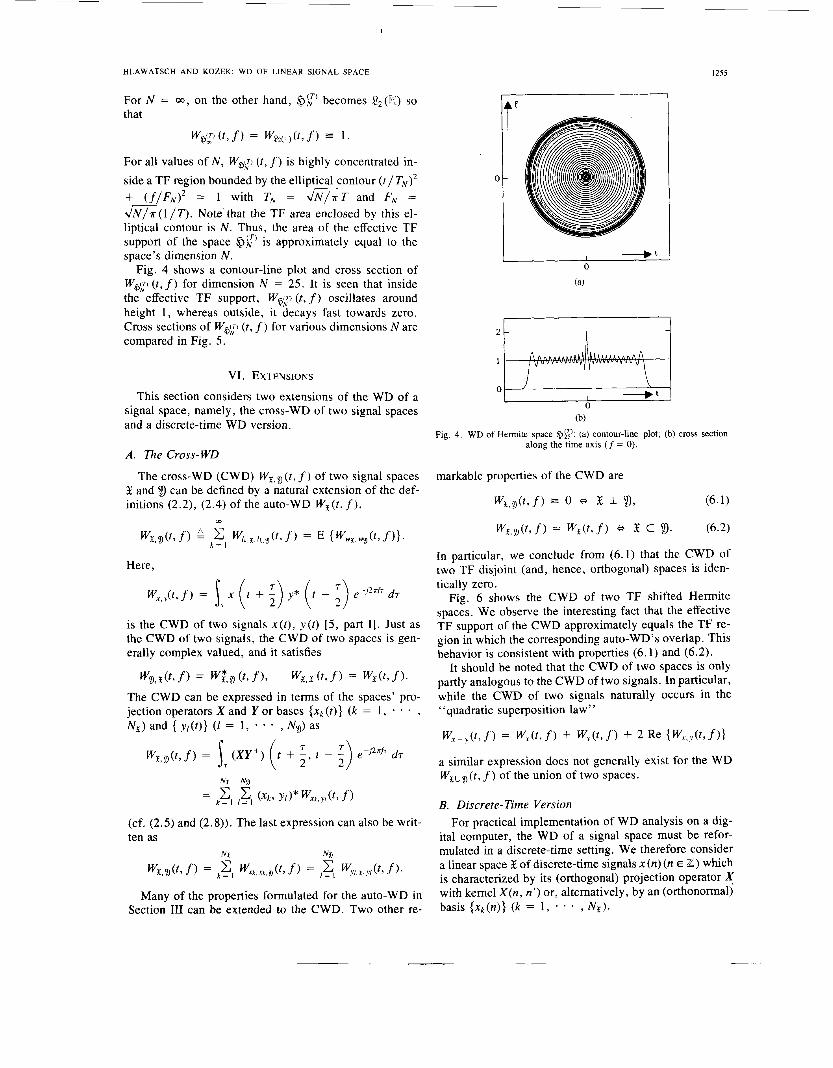
For all values of N , WQa) ( t , f ) is highly concentrated inside a TF region bounded by the elliptical contour ( t / TN)2 + ( f / F N ) 2 = 1 with T, = a T and FN =

m ( l / T ) . Note that the TF area enclosed by this elliptical contour is N . Thus, the area of the effective TF support of the space $jr) is approximately equal to the space’s dimension N .

Fig. 4 shows a contour-line plot and cross section of W@g) ( t , f ) for dimension N = 25. It is seen that inside the effective TF support, W@jy~) (t, f ) oscillates around height 1, whereas outside, it decays fast towards zero. Cross sections of W@g) ( t , f ) for various dimensions N are compared in Fig. 5.

VI. EXTENSIONS

This section considers two extensions of the WD of a signal space, namely, the cross-WD of two signal spaces and a discrete-time WD version.

A. The Cross-WD

The cross-WD (CWD) Wx,Ig( t , f ) of two signal spaces X and 9 can be defined by a natural extension of the definitions (2.2), (2.4) of the auto-WD W x ( t , f ) ,

m

Wx,(r ( t? f ) ’ W / A x./A v ( r > f ) E { W W x , W g ( t 7 f)]. k = I

Here,

is the CWD of two signals x ( t ) , y ( t ) [5, part I]. Just as the CWD of two signals, the CWD of two spaces is generally complex valued, and it satisfies

W9,x(t, f ) = w;,, (t, f), Wx,z ( t , f ) = Wx(t, f ) . The CWD can be expressed in terms of the spaces’ projection operators X and Y or bases { x k ( t ) } ( k = 1, * * * , N , ) and { y , ( t ) } (1 = 1, , NIg) as

N I Nn

(cf. (2.5) and (2.8)). The last expression can also be written as

NI ,?I

~ x , r g ( t , f ) = ,C, ~ x i , x A . g ( t , f ) = ~ y , , x . y , ( t , f ) .

Many of the properties formulated for the auto-WD in Section 111 can be extended to the CWD. Two other re-

0

Cf

I I

I --+t o J

0 (b)

Fig. 4. WD of Hermite space 4:;’: (a) contour-line plot; (b) cross section along the time axis (f = 0).

markable properties of the CWD are

W x , v ( t , f ) = W x ( t , f ) e X C 9. (6.2)

In particular, we conclude from (6.1) that the CWD of two TF disjoint (and, hence, orthogonal) spaces is identically zero.

Fig. 6 shows the CWD of two TF shifted Hermite spaces. We observe the interesting fact that the effective TF support of the CWD approximately equals the TF region in which the corresponding auto-WD’s overlap. This behavior is consistent with properties (6.1) and (6.2).

It should be noted that the CWD of two spaces is only partly analogous to the CWD of two signals. In particular, while the CWD of two signals naturally occurs in the ‘‘quadratic superposition law”

w x + , ( t , f ) = W,(t,f) + w,@,f> + 2 Re { W x , y ( t , f ) }

a similar expression does not generally exist for the WD Wx,,(t, f ) of the union of two spaces.

B. Discrete- Time Version For practical implementation of WD analysis on a dig-

ital computer, the WD of a signal space must be reformulated in a discrete-time setting. We therefore consider a linear space X of discrete-time signals x (n) (n E Z) which is characterized by its (orthogonal) projection operator X with kernel X ( n , n’) or, alternatively, by an (orthonormal) basis { x k ( n ) } ( k = 1, * * , N , ) .

I

1256 IEEE TRANSACTIONS ON SIGNAL PROCESSING, VOL. 41, NO. 3, MARCH 1993

N = S - TI N = 6 4 2 1

I I

Fig. 5 . Cross sections of W & l ( ? . f ) along the time axis (f = 0) for various dimensions N

t ' r f I c--_ .

\

Fig. 6 . Cross-WD of two time-frequency shifted Hermite spaces X, '1, (both with dimension N = 16): (a) auto-WD of space X; (b) auto-WD of space '1,; (c) magnitude of cross-WD of spaces X, 9.

Using the discrete-time WD of a signal x ( n ) [5 , part 111 W D , x ( n , e> = 2 C X ( n + m, n - m)e-J4nem m

it is straightforward to reformulate the definitions (2.2), (2.4) of the WD of a space in the discrete-time setting considered here. We then obtain the following expressions for the discrete-time WD of a discrete-time space X :

(cf. (2.6), (2.8)). We note that, just as the discrete-time WD of a signal (see (6.3)), W D , x ( n , 0) is periodic with respect to the normalized-frequency variable 8 with pe-

I

HLAWATSCH AND KOZEK: WD OF LINEAR SIGNAL SPACE

nod 1, i .e., one half of the spectral period 1 of discrete- time signals. This will cause aliasing effects unless all elements x ( n ) of the space X are band limited in some fixed “halfband” [eo, Bo + i]. In other words, aliasing is avoided if X C S j , where S j denotes the “halfband subspace” of all signals satisfying the above band-limitation property with fixed Bo.

According to (6.5), WD,x(n , 0) can be calculated by adding the WD’s of all basis signals xk(n). A more effi- cient implementation is obtained by first forming the projection operator kernel

NI

X ( n , n’) = ,Cl xk(n>-GYn’>

and then applying an FFT to compute a discrete-frequency version of the Fourier transform (6.4).

VII. DISCUSSION AND CONCLUSION The Wigner distribution (WD) of a linear signal space

has been defined by suitably averaging the WD’s of the space’s elements. The interpretation of the WD of a space as the space’s time-frequency (TF) energy distribution is supported by its definition, its properties, and the results obtained for specific spaces. However, just as in the case of TF signal analysis, a pointwise interpretation of the WD of a space as joint T F energy density is impossible due to fundamental resolution limitations imposed by the uncertainty principle.

Since any quadratic signal representation can be reformulated for a space as discussed in Section 11-E, it is clear that the TF analysis of signal spaces may be based on other (quadratic) TF representations as well. For example, the Rihaczek distribution [ 5 , part 1111 of a space could be used instead of the WD. However, it is well known that the WD of a signal has specific advantages over alternative T F signal representations. One of these advantages is the fact that the WD, among a class of TF representations with similar mathematical properties, features optimum TF concentration [ 191. Both from the definitions (2.2), (2.4) and the expression (2.8), it is evident that the optimum TF concentration featured by the WD of a signal directly carries over to the WD of a space.

In the signal case, some smoothing is often applied to the WD in order to reduce the WD’s oscillatory interference terms 161, [15], [20]. Although any smoothed WD version (such as the smoothed pseudo-WD, the spectrogram, or the Choi-Williams distribution) can be redefined for a space as discussed in Section 11-E, a smoothing of the WD is usually not an imperious necessity in the case of a signal space since the WD of a space typically shows only a moderate amount of interference. This can be at- tributed to the “averaging” operation inherent in the WD of a space (see (2.2), (2.4), (2.8)) which can often be viewed as an implicit smoothing.

While the WD of a signal space has been introduced in this paper as a tool for the TF analysis of signal spaces, it also provides a basis for the TF synthesis of signal spaces. This, in turn, allows the design of “TF projection

1251

filters” which are linear, time-varying filters (projections) with specified T F pass region. This concept, its extension to perfect-reconstruction filter banks, and a computation- ally attractive approximate design method, are discussed in [21]. In [22], the WD of a signal space is extended to the TF analysis and synthesis of linear, time-varying systems. Finally, the ambiguity function of a linear signal space and its application to the maximum-likelihood estimation of range and Doppler shift are discussed in [23].

APPENDIX In this Appendix, we derive the WD expression (2.5)

from the WD definition (2.2) or (2.4). Starting from definition (2.2) and interchanging the summation and the in- tegration, we obtain

= i,, X ( t , , t ’ )X*( t2 , t ’ ) dt‘

where we have used (1.2) and (2. la). Expression (2.5) is obtained by inserting (A.2) into (A. 1).

The derivation based on definition (2.4) instead of definition (2.2) is strictly analogous; it suffices to replace lk (t) by w ( t ) and the summation over k by the expectation E, and use (2.3a) instead of (2.la).

REFERENCES

[ 11 L. E. Franks, Signal 7heory. Englewood Cliffs, NJ: Prentice-Hall,

[ 2 ] A. W. Naylor and G . R . Sell, Linear Operator Theory in Engineering 1969.

and Science. Springer-Verlag, 1982.

I

L. L. Scharf, Statistical Signal Processing. Addison-Wesley, Read- ing, MA, 1990. F. Hlawatsch and W. Kozek, “Time-frequency analysis of linear signal spaces,” in Proc. IEEE 1991 In?. Conf. Acoust., Speech, Signal Processing (/CASSP-91), Toronto, Canada, May 1991, pp. 2045- 2048. T. A. C. M. Claasen and W. F. G. Mecklenbrauker, “The Wigner distribution-a tool for time-frequency signal analysis,” Parts 1-111, Philips J . Res. , vol. 35, pp. 217-250, 276-300, 372-389; 1980. F. Hlawatsch and P. Flandrin, “The interference structure of the Wigner distribution and related time-frequency signal representations,” in The Wigner Distribution-Theory and Applications in Sig- nal Processing, W. Mecklenbrauker, Ed. Elsevier Science Publish- ers, to be published 1993. W. Martin and P. Flandrin, “Wigner-Ville spectral analysis of non- stationary processes,” IEEE Trans. Acoust. , Speech, Signal Process- ing, vol. ASSP-33, pp. 1461-1470, Dec. 1985. P. Flandrin and W. Martin, “The Wigner-Ville spectrum of nonsta- tionary random signals, ” in The Wigner Distribution-Theory and Applications in Signal Processing, W . Mecklenbrauker, Ed. Elsev- ier Science Publishers, to be published, 1993. G . B. Folland, Harmonic Analysis in Phase Space. Princeton Uni- versity Press, 1989. A. J . E. M. Janssen, “Wigner weight functions and Weyl symbols of nonnegative definite linear operators,” Philips J . Res. , vol. 44,

W. Kozek and F. Hlawatsch, “Time-frequency representation of linear time-varying systems using the Weyl symbol,’’ in Proc. IEE 6th Int. Conf. Digital Processing Signals Commun., Loughborough, U.K., Sept. 1991, pp. 25-30. F. Hlawatsch, “Regularity and unitarity of bilinear time-frequency signal representations,” IEEE Trans. Inform. Theory, vol. 38, pp, 82-94, Jan. 1992. E. P. Wigner, “Quantum-mechanical distribution functions revis- ited,” in Perspectives in Quantum Theory, W. Yourgrau and A. van der Merwe, Eds. F. Hlawatsch, “Duality and classification of bilinear time-frequency signal representations,” IEEE Trans. Signal Processing, vol. 39, pp. 1564-1574, July 1991. F . Hlawatsch and G. F. Boudreaux-Bartels, “Linear and quadratic time-frequency signal representations,” IEEE Signal Processing Map.. Apr. 1992.

pp. 7-42, 1989.

New York: Dover, 1971.

IEEE TRANSACTIONS ON SIGNAL PROCESSING, VOL. 41, NO. 3, MARCH 1993

[I61 B. ?. K.-Kumar and K. J. deVos, “Linear system description using Wigner distribution functions,” Proc. SPIE Int. Soc. Opt. Eng., vol.

1171 N. G. de Bruijn, “Uncertainty principles in Fourier analysis,” in New York: Academic, 1967, pp. 57-

826, pp. 115-124, 1987.

Inequalities, 0 . Shisha, Ed. 71.

M. Abramowitz and I. A. Stegun, Handbook of Mathematical Func- tions. New York: Dover, 1965. A. J . E. M. Janssen, “On the locus and spread of pseudodensity functions in the time-frequency plane,” PhilipsJ. Res. , vol. 37, pp. 79- 110, 1982. P. Flandrin, “Some features of time-frequency representations of multicomponent signals,” in Proc. IEEE 1984 Int. Conf. Acoust., Speech, Signal Processing (ICASSP-84), San Diego, CA, Mar. 1984, pp. 4 1 B .4.1-4 1B .4.4. W. Kozek and F. Hlawatsch, “Time-frequency filter banks with perfect reconstruction,” in Proc. IEEE 1991 lnt. Conf. Acoust., Speech, Signal Processing (ICASSP-92), Toronto, Canada, May 1991, pp.

F. Hlawatsch, “Wigner distribution analysis of linear, time-varying systems,” in Proc. IEEE 1992 Int. Symp. Circuits Syst. (ISCAS-92), San Diego, CA, May 1992, pp. 1459-1462. F. Hlawatsch and G . S. Edelson, “The ambiguity function of a linear signal space and its application to maximum-likelihood range/Dop- pler estimation,” in Proc. IEEE SP Int. Symp. Time-Frequency Time- Scale Analysis, Victoria, B.C., Canada, Oct. 1992,pp. 489-492.

2049-2052.

Franz Hlawatsch (S’85-M’88) received the Di- plom-Ingenieur and Dr. techn. degrees in electrical engineering from the Vienna University of Technology, Austria, in 1983 and 1988, respectively.

Since 1983 he has been a Research and Teach- ing Assistant at the Department of Communica- tions and Radio-Frequency Engineering, Vienna University of Technology. In 1991 he spent a sab- batical year at the Department of Electrical En- gineering, University of Rhode Island, Kingston,

RI. His research interests are in signal theory and signal processing with emphasis on time-frequency methods.

Werner Kozek (S’92) received the Diplom-In- genieur degree in electrical engineering from the Vienna University of Technology, Austria, in 1990.

Since 1990 he has been a Research Assistant at the Department of Communications and Radio- Frequency , Engineering, Vienna University of Technology. His research interests are in signal processing with emphasis on time-varying systems.

franz hlawatsch, member, ieee, and werner kozek, … · i i248 ieee transactions on signal...

Documents