frame capture in iee e 802.11p vehicular...
TRANSCRIPT

MASTER THESIS
FRAME CAPTURE IN IEEE 802.11P VEHICULAR NETWORKS A SIMULATION-BASED APPROACH
P. van Wijngaarden, B.Sc FACULTY OF ELECTRICAL ENGINEERING, MATHEMATICS AND COMPUTER SCIENCE DESIGN AND ANALYSIS OF COMMUNICATION SYSTEMS EXAMINATION COMMITTEE dr. ir. G. Heijenk dr. ir. G. Karagiannis E.M. van Eenennaam, M.Sc.
JULY 2011

ii

Abstract
This thesis describes the occurrence of Frame Capture in the IEEE 802.11p physicallayer. Frame Capture occurs when two nodes simultaneously transmit a message (aPLCP frame) that spatially and temporally overlaps at a certain receiver, creating acollision. Collisions can occur because of hidden terminals, or because of simultaneouslyending backoff counters between coordinated nodes. If both frames are equal in signalstrength, they both interfere in such a degree with each other that the receiver will not beable to decode either one of them. However, if one frame is received with a significantlyhigher power level than the other, the receiver can (under some conditions) be able tosuppress the weaker frame and correctly receive the stronger one.
We studied the available literature on Frame Capture and concluded that the capturebehavior is different among various chipsets and depends largely on the arrival timedifference (in the order of microseconds) between both frames and on whether bothframes interfere in each other’s PLCP preamble or not. The literature compares Atherosand Prism chipsets, and demonstrates that if the stronger frame arrives before the weakerframe, both chipset types are able to capture the frame if the signal to noise ratio ishigh enough. If the stronger frame arrives later, the required SNR is significantly higherbecause the receiver must be able to clearly hear the stronger frame’s preamble, even inthe presence of interference, to lock onto the new frame correctly.
We implemented this capture behavior in our wireless network simulator, OMNeT++with the MiXiM module, with the use of capture thresholds. Depending on the momentof arrival and the current state of the receiver, a certain threshold must be exceededfor the receiver to capture the frame. These capture thresholds are based on the resultsin the literature, but could be refined later on with experiments of our own. Note thatcapturing the frame (which happens after the preamble) does not guarantee correctreception: if for example during the frame more interference arrives, the frame can stillbe lost.
We also enhanced the bit error calculation & prediction formulas in MiXiM, which whereonly suited for 802.11b, a completely different physical layer. We now approximate biterrors with theoretical formulas derived for an AWGN channel (i.e. where white noiseis the only interference). This is not perfect yet but a significant improvement over thecurrent implementation, and it will help further increase the channel model accuracy inthe future.
iii

After the implementation work was complete, we performed simulations of vehicularnetworks with which we demonstrate that Frame Capture is especially important invehicular networks with broadcast traffic. This is because the hidden terminal problembecomes more prevalent when all frames are broadcast, because the standard RTS/CTSmechanism can not be used to warn hidden terminals about ongoing transmissions. Wedemonstrate that both Atheros and Prism chipsets show a performance gain of at least20% over (reference) chipsets which do not perform any kind of Frame Capture. Byartificially disabling the hidden terminal problem (i.e. silencing all hidden terminalsduring a transmission) we show that Frame Capture is mostly important when resolvinghidden terminal collisions. Collisions between coordinated nodes are more likely to havean equal power level and can usually not be resolved with Frame Capture. Becausenodes do not update their MAC contention window if broadcast traffic is the only typeof traffic in the network, occurrence of collisions between coordinated nodes increaseswith increased node density.
iv

Samenvatting
Dit onderzoekt beschrijft Frame Capture in de fysieke laag van IEEE 802.11p. FrameCapture treedt op wanneer twee nodes tegelijkertijd een bericht (een PLCP frame) sturennaar een derde node. Dit creeert een collision, ofwel een botsing tussen twee frames.Collisions kunnen optreden door hidden terminals (als de twee zendende nodes elkaarniet kunnen horen), of door backoff timers (van de IEEE 802.11 MAC laag) die tegeli-jkertijd aflopen, waardoor ze op precies hetzelfde moment beginnen te zenden. Als deframes ongeveer dezelfde signaalsterkte hebben zijn beide transmissies doorgaans ver-loren gegaan, maar dit hoeft niet altijd het geval te zijn; als een van de twee een sig-naalsterkte heeft die significant sterker is dan de andere, kan de ontvanger soms tochhet sterkere frame succesvol ontvangen. Dit wordt ’Frame Capture’ genoemd.
We hebben de beschikbare literatuur over Frame Capture bestudeerd en geconcludeerddat het capture gedrag verschilt tussen de chipsets van verschillende fabrikanten. Dezeverschillen kunnen hun effect hebben op de performance van het gehele netwerk. Of eenontvanger in staat is om een frame te capturen hangt af van de signaal-ruisverhoudingen het verschil in aankomsttijd (in de orde van microseconden); als de ontvanger (veel)interferentie heeft tijdens de preamble, wordt de kans op succes kleiner. Op dit puntverschillen Atheros en Prism chipsets ook van elkaar: Prism chipsets zijn alleen maar instaat om een sterker frame te capturen als het eerder aankomt dan het zwakkere frame,terwijl Atheros chipsets ook een sterker frame kunnen capturen terwijl de ontvanger albegonnen is met het ontvangen van het zwakkere frame. Afhankelijk van de status vande ontvanger en of de ontvanger nog meer interferentie heeft of niet, is de vereiste SNR(signal-to-noise ratio of signaal-ruis verhouding) hoger resp. lager.
We hebben dit capture gedrag geimplementeerd in onze netwerksimulator, het OM-NeT++ framework met de MiXiM module. We gebruiken capture thresholds, dit zijnSNR waarden die een frame moet hebben om in het geval van een collision gecapturedte kunnen worden. Deze thresholds zijn gebaseerd op de resultaten van experimentenuit de literatuur, maar zouden later verbeterd of gevalideerd kunnen worden met eigenexperimenten met IEEE 802.11p hardware. Let op dat het capturen van een frame nietautomatisch leidt tot succesvolle ontvangst: afhankelijk van de hoeveelheid interferentiedie de ontvanger heeft tijdens het data-gedeelte van het frame zou het frame nog steedsverloren kunnen gaan.
We hebben ook de bit error berekenings- & voorspellings-formules verbeterd in MiXiM.
v

Deze waren eerst gebaseerd op 802.11b, wat een geheel andere fysieke laag is (gebaseerdop DSSS). We benaderen bitfouten nu met behulp van theoretische formules die bit- enpakketfouten benaderen voor een AWGN-kanaal (met alleen witte ruis als interferen-tiebron). Dit is niet perfect en er zijn in het echt veel meer effecten die een rol spelen,maar deze benadering is in ieder geval een verbetering ten opzichte van de oude situatieen een stap voorwaarts richting een beter model voor het kanaal in de toekomst.
Nadat de implementatie voltooid en gevalideerd was, hebben we simulaties van au-tonetwerken uitgevoerd die demonstreren dat Frame Capture inderdaad een belangri-jke positieve bijdrage levert aan de performance van een netwerk met hoofdzakelijkbroadcast-verkeer. Dit komt doordat het hidden terminal probleem een grotere rol speeltin autonetwerken, omdat het standaard RTS/CTS mechanisme dat gebruikt wordt omcollisions te voorkomen niet gebruikt kan worden bij broadcasts.
We hebben laten zien dat zowel Atheros als Prism chipsets minimaal 20% beter presterendan een gewone chipset (ter referentie) met geen enkele vorm van Frame Capture. Ookpresteren Atheros chipsets altijd tussen de 5 en 8% beter dan de Prism chipsets, dankzijhet feit dat ze op elk willekeurig moment een frame kunnen capturen, niet alleen vooren tijdens de preamble van het zwakkere frame.
Door kunstmatig het hidden terminal probleem uit te schakelen (d.w.z. door te zorgendat alle hidden terminals toch op de hoogte zijn van transmissies die gaande zijn) hebbenwe kunnen laten zien dat Frame Capture vooral belangrijk is bij het oplossen van colli-sions met hidden terminals. Collisions tussen coordinated nodes (nodes die dichter bijelkaar staan en elkaar wel kunnen horen) hebben meestal een signaalsterkte die min ofmeer gelijk is en kunnen daarom veel minder vaak door Frame Capture opgelost worden.Daarnaast hebben we kunnen laten zien dat de verhoogde coordinatie van nodes (dehidden terminals die stil zijn) er zelfs voor zorgt dat de performance van het netwerkiets afneemt omdat alle collisions tussen coordinated nodes zullen zijn, en deze niet doorFrame Capture opgelost kunnen worden.
vi

Acknowledgements
The road towards the work lying before you today has not always been paved withgold. A long time ago I started with the preliminary research for this thesis, while alsoworking 2 days per week at a company and trying to do another Masters (the one inComputer Security). This proved to be very unfertile ground for decent and productiveresearch, and it was only after I quit my job and stopped with my second Masters thatmy work on vehicular networks could really start. After that I fell into numerous otherpitfalls that come with a research as big as this - I did not clearly define the scope of mywork, leading me to investigate branch after branch of related topics - with the channelmodeling and signal theory as the most time-consuming examples. However, after a yearof hard work I’m proud of the result you have in your hands right now.
This work however would not have come to fruition if it were not for the people aroundme. I would like to thank my supervisors and professors Martijn, Geert and Georgios fortheir support all these months, their insights and guidance has always helped me steerin the right direction. In the early stages of my research Mark Bentum took the timeto explain how to look at OFDM and what made these carriers exactly ’orthogonal’, forwhich I owe him many thanks.
The people from the OMNeT++ Google Group have helped with the implementationissues I faced from time to time, thanks to a platform like Google Groups many peopleare helped forward with anything they might encounter.
Last but certainly not least, my gratitude goes out to my parents who always helpedto motivate me and supported me financially during all these years that I receivededucation, and my family and friends.
So long.. and thanks for all the fish!
vii

viii
Contents
1 Introduction 7
1.1 Problem statement . . . . . . . . . . . . . . . . . . . . . . . . . . . . . . . 8
1.2 Research questions . . . . . . . . . . . . . . . . . . . . . . . . . . . . . . . 9
1.3 Outline . . . . . . . . . . . . . . . . . . . . . . . . . . . . . . . . . . . . . 10
2 IEEE 802.11 11
2.1 Basics . . . . . . . . . . . . . . . . . . . . . . . . . . . . . . . . . . . . . . 11
2.2 Medium Access Control . . . . . . . . . . . . . . . . . . . . . . . . . . . . 12
2.3 OFDM . . . . . . . . . . . . . . . . . . . . . . . . . . . . . . . . . . . . . . 15
2.3.1 Introduction . . . . . . . . . . . . . . . . . . . . . . . . . . . . . . 15
2.3.2 OFDM mathematics . . . . . . . . . . . . . . . . . . . . . . . . . . 16
2.3.3 Preamble detection . . . . . . . . . . . . . . . . . . . . . . . . . . . 18
2.3.4 Guard times, coding and forward error correction . . . . . . . . . . 18
2.3.5 Strengths and weaknesses of OFDM . . . . . . . . . . . . . . . . . 21
2.3.6 OFDM transmission and reception blocks . . . . . . . . . . . . . . 22
2.4 BER Calculations . . . . . . . . . . . . . . . . . . . . . . . . . . . . . . . . 23
3 Vehicular Networks 29
3.1 Basics . . . . . . . . . . . . . . . . . . . . . . . . . . . . . . . . . . . . . . 29
3.2 Applications . . . . . . . . . . . . . . . . . . . . . . . . . . . . . . . . . . . 30
3.3 Challenges . . . . . . . . . . . . . . . . . . . . . . . . . . . . . . . . . . . . 31
3.4 IEEE 802.11p . . . . . . . . . . . . . . . . . . . . . . . . . . . . . . . . . . 32
3.4.1 Physical layer . . . . . . . . . . . . . . . . . . . . . . . . . . . . . . 32
3.4.2 Effects of changes at the physical layer . . . . . . . . . . . . . . . . 33
4 Frame Capture 35
4.1 What is it . . . . . . . . . . . . . . . . . . . . . . . . . . . . . . . . . . . . 35
4.1.1 Related work . . . . . . . . . . . . . . . . . . . . . . . . . . . . . . 35
4.1.2 When does it occur . . . . . . . . . . . . . . . . . . . . . . . . . . . 36
4.1.3 How does it work . . . . . . . . . . . . . . . . . . . . . . . . . . . . 36
4.1.4 Frame Capture in other communication systems . . . . . . . . . . 37
4.2 Scenarios . . . . . . . . . . . . . . . . . . . . . . . . . . . . . . . . . . . . 38
4.3 Simulation . . . . . . . . . . . . . . . . . . . . . . . . . . . . . . . . . . . . 41
4.4 Potential impact . . . . . . . . . . . . . . . . . . . . . . . . . . . . . . . . 42
1

CONTENTS CONTENTS
5 OMNeT++ and MiXiM 455.1 Discrete-event network simulation . . . . . . . . . . . . . . . . . . . . . . . 455.2 Requirements . . . . . . . . . . . . . . . . . . . . . . . . . . . . . . . . . . 46
5.2.1 Environment . . . . . . . . . . . . . . . . . . . . . . . . . . . . . . 465.2.2 Node movement . . . . . . . . . . . . . . . . . . . . . . . . . . . . 46
5.3 OMNeT++ . . . . . . . . . . . . . . . . . . . . . . . . . . . . . . . . . . . 475.4 MiXiM . . . . . . . . . . . . . . . . . . . . . . . . . . . . . . . . . . . . . . 48
5.4.1 Environmental models . . . . . . . . . . . . . . . . . . . . . . . . . 485.4.2 Wireless channel models . . . . . . . . . . . . . . . . . . . . . . . . 495.4.3 Physical layer . . . . . . . . . . . . . . . . . . . . . . . . . . . . . . 49
6 Implementation 576.1 Frame Capture . . . . . . . . . . . . . . . . . . . . . . . . . . . . . . . . . 57
6.1.1 Justification of capture thresholds . . . . . . . . . . . . . . . . . . 596.2 BER calculations . . . . . . . . . . . . . . . . . . . . . . . . . . . . . . . . 606.3 Validation . . . . . . . . . . . . . . . . . . . . . . . . . . . . . . . . . . . . 63
6.3.1 Setup of the experiment . . . . . . . . . . . . . . . . . . . . . . . . 646.3.2 Difficulties . . . . . . . . . . . . . . . . . . . . . . . . . . . . . . . . 646.3.3 Expected results . . . . . . . . . . . . . . . . . . . . . . . . . . . . 666.3.4 Results . . . . . . . . . . . . . . . . . . . . . . . . . . . . . . . . . 67
7 Simulations 697.1 Simulation plan . . . . . . . . . . . . . . . . . . . . . . . . . . . . . . . . . 70
7.1.1 Road vehicle density . . . . . . . . . . . . . . . . . . . . . . . . . . 707.1.2 Traffic generation rate . . . . . . . . . . . . . . . . . . . . . . . . . 727.1.3 Node chain length . . . . . . . . . . . . . . . . . . . . . . . . . . . 72
7.2 Basic parameters . . . . . . . . . . . . . . . . . . . . . . . . . . . . . . . . 727.2.1 Multi-lane . . . . . . . . . . . . . . . . . . . . . . . . . . . . . . . . 747.2.2 Hidden Terminal Problem . . . . . . . . . . . . . . . . . . . . . . . 74
7.3 Metrics . . . . . . . . . . . . . . . . . . . . . . . . . . . . . . . . . . . . . 757.4 Results . . . . . . . . . . . . . . . . . . . . . . . . . . . . . . . . . . . . . . 78
7.4.1 Single Lane . . . . . . . . . . . . . . . . . . . . . . . . . . . . . . . 787.4.2 Multi Lane . . . . . . . . . . . . . . . . . . . . . . . . . . . . . . . 827.4.3 Hidden Terminal Problem . . . . . . . . . . . . . . . . . . . . . . . 85
8 Conclusions 91
9 Future work 93
A Channel effects 105
B Orthogonality of multiple sinusoidals and their frequency spacing 107
2

List of Figures
2.1 The IEEE 802 Networking Family . . . . . . . . . . . . . . . . . . . . . . 12
2.2 The IEEE 802 Distributed Coordination Function . . . . . . . . . . . . . 13
2.3 Simplified visualization of the hidden terminal problem. . . . . . . . . . . 14
2.4 Orthogonality of subcarriers in the frequency domain . . . . . . . . . . . . 15
2.5 BPSK and QAM constellations . . . . . . . . . . . . . . . . . . . . . . . . 16
2.6 The Fourier transform of the rectangular pulse . . . . . . . . . . . . . . . 17
2.7 802.11 OFDM channel structure . . . . . . . . . . . . . . . . . . . . . . . 17
2.8 PLCP Frame and Preamble diagrams . . . . . . . . . . . . . . . . . . . . 19
2.9 Cyclic prefix extension . . . . . . . . . . . . . . . . . . . . . . . . . . . . . 20
2.10 An example of a convolutional encoder . . . . . . . . . . . . . . . . . . . . 21
2.11 OFDM transceiver block diagram . . . . . . . . . . . . . . . . . . . . . . . 22
2.12 Convolutional encoder from IEEE 802.11a and 802.11p . . . . . . . . . . . 25
2.13 Numerical results for QAM packet error probabilities . . . . . . . . . . . . 27
3.1 BER curves for uncoded BPSK with 802.11a and 802.11p. . . . . . . . . 34
4.1 Required SNR for various Frame Capture scenarios . . . . . . . . . . . . . 40
5.1 OMNeT++ module structure . . . . . . . . . . . . . . . . . . . . . . . . . 48
5.2 MiXiM physical layer functionality diagram . . . . . . . . . . . . . . . . . 51
5.3 MiXiM physical layer transmission flow diagram . . . . . . . . . . . . . . 52
5.4 MiXiM reception functionality blocks . . . . . . . . . . . . . . . . . . . . . 54
5.5 802.11b and 802.11p PER curves at their lowest bit rates (1 and 3Mbps) . 55
6.1 MiXiM Decider - enhancements made to enable Frame Capture . . . . . . 60
6.2 Comparison of the approximation function with the sampled function forBPSK (code rate 1/2) from Figure 2.13. . . . . . . . . . . . . . . . . . . . 62
6.3 Validation experiment setup . . . . . . . . . . . . . . . . . . . . . . . . . . 65
6.4 Required SNR for Frame Capture where strongest frame arrives first . . . 65
6.5 Comparison of Frame Capture experimental results, and the estimatedresults based on our implementation . . . . . . . . . . . . . . . . . . . . . 66
6.6 Frame Capture validation simulation results . . . . . . . . . . . . . . . . . 68
7.1 The relationship between low node density and hidden terminal problem. 71
3

LIST OF FIGURES LIST OF FIGURES
7.2 The relationship between high node density and the hidden terminal prob-lem. (S = Sender, R = Receiver, Q = Quiet, H = Hidden) . . . . . . . . . 71
7.3 Collision probability for single-lane scenarios . . . . . . . . . . . . . . . . 787.4 Beacon success probabilities for th singe-lane scenarios. . . . . . . . . . . 797.5 Capture Factor for the single-lane scenarios . . . . . . . . . . . . . . . . . 817.6 Collision probability for single- and multi-lane (4 lanes) scenarios . . . . . 827.7 Beacon success probability comparison for the multi lane scenarios, all
with 802.11p bit error calculations. . . . . . . . . . . . . . . . . . . . . . . 837.8 Capture Factor for the multi-lane scenarios. . . . . . . . . . . . . . . . . . 847.9 Collision probability in the scenarios without hidden terminals . . . . . . 867.10 Beacon success probability in the scenario without hidden terminal colli-
sions. The upper two lines belong to the single-lane scenarios. . . . . . . . 877.11 Comparison of the Capture Factor in the normal scenario and without
hidden terminal collisions. The upper two lines belong to the multi-lanescenarios. . . . . . . . . . . . . . . . . . . . . . . . . . . . . . . . . . . . . 88
4

List of Tables
2.1 801.11a data rates and modulations / coding rates [1] . . . . . . . . . . . 23
3.1 802.11a and 802.11p PHY values [2] . . . . . . . . . . . . . . . . . . . . . 33
4.1 Frame Capture scenarios (data rate of 6 Mbps). These timing relationsand results are for Atheros chipsets [3]. The experiments were performedwith 802.11a. . . . . . . . . . . . . . . . . . . . . . . . . . . . . . . . . . . 39
4.2 Bit Error Rate calculation methods in various simulators . . . . . . . . . . 43
7.1 Frame Capture simulation scenarios . . . . . . . . . . . . . . . . . . . . . 897.2 Simulation scenarios (numbers indicate # repetitions) . . . . . . . . . . . 897.3 Simulation metrics . . . . . . . . . . . . . . . . . . . . . . . . . . . . . . . 90
5

LIST OF TABLES LIST OF TABLES
6

1Introduction
Nowadays, mobility and transport have become vital aspects of our society. Almosteverybody has a car parked in front of their house or in their garage, which is usedeveryday - to get to work, to bring kids to school and pick them up, to visit family andfriends, to buy groceries. . . these are just a few typical examples of how much we havegotten used and attached to our increased mobility and the convenience of owning a car.It is not even a luxury anymore; everybody has a car these days. With an increasingeconomy, both goods and people tend to move around a lot more and a lot faster thanbefore, and the infrastructures we need to support that mobility are always expanding.But even though the infrastructure expands, it happens often that its capacity is notsufficient.
The traffic density on the Dutch highways is enormous, not just around the big cities,and on average working days there are over 200 km of traffic jams. This is about 4% ofthe entire Dutch highways network. Peaks in congestion due to weather conditions canrise up to 800 kilometers. The Dutch Ministry of Transport, Public Works and WaterManagement calculated that the annual economical damage because of traffic jams wasbetween 2,8 and 3,6 billion euros in 2008. This was an increase of 7 percent comparedto 2007, and even a 78 percent increase compared to 2000 [4]. These costs include bothdirect and indirect economical damage like extra fuel usage, the implied environmentalfootprint and commuters arriving late at work which causes companies to lose time andmoney. This does not only apply to the Dutch highways however, all growing societiesaround the globe suffer from heavy traffic congestion at peak hours.
Many solutions to this problem have been proposed. Usage of the roads is being taxed,people have been motivated to travel together instead of separately (also known as
7
1.1. PROBLEM STATEMENT CHAPTER 1. INTRODUCTION
carpooling) and in the Netherlands a system called rekeningrijden or ’billed driving’ hasbeen proposed to distribute the infrastructure maintenance costs more evenly over thepeople who actually use it. However, none of these solutions actually try to increase thecapacity that the roads in terms of ’passing vehicles per hour’ can sustain.
Vehicular networks try to fill that gap. By creating networks between vehicles, all usersof the roads could have increased knowledge about the ’state’ of the road, the currentamount of traffic and the speed at which the traffic on it travels. This information canthen be used to increase the safety on the roads and the capacity, leading to less trafficcongestion, reduced emissions and reduced costs.
This research does not cover the entire challenge of how vehicular networks can makeour lives a bit easier, but merely a few of the aspects of it; we look at some of thechallenges presented when simulating vehicular networks. Many application protocolsand systems that are to be used in vehicular networks must of course be tested first, atdifferent stages during their development. Simulation of these applications and protocolsis an important step in this process. We can learn a lot about the expected behaviorand find out how things would function and whether they are scalable without imple-menting all functionality in real cars. Also, simulations reduce the need for testing thebehavior on circuits or blocking stretches of the highway, which is of course an expensiveundertaking.
1.1 Problem statement
This thesis thus focuses mainly on the simulation of the physical layer in vehicular net-works. We give special attention to one problem in particular: Frame Capture. FrameCapture happens when two nodes try to send a frame to a third one at the same timeand at the same frequency, i.e. when a collision occurs. Under some circumstances (de-pending on the signal to noise ratio’s and the arrival times of both) the receiver is ableto capture one of both frames, instead of losing them both because of the collision. Thisbecame the first important question that we tried to answer: How does Frame Capturework exactly? We looked at the knowledge that was already available and performed aliterature study on three topics: basic IEEE 802.11 networks, the typical IEEE 802.11physical layers and on Frame Capture. We looked specifically at the 802.11a and 802.11pphysical layers because they are both based on Orthogonal Frequency Division Multi-plexing (OFDM). As can be read later in Chapter 3.4, IEEE 802.11p is the variety thatis used for vehicular networks, which makes it the most important physical layer for us.Based on that literature study, the following observations came to the surface:
• Frame Capture behaves differently on chipsets of different manufacturers [5, 6, 3].
• Because of its nature, Frame Capture probably occurs often in vehicular networkswith a lot of broadcast traffic.
8

CHAPTER 1. INTRODUCTION 1.2. RESEARCH QUESTIONS
Much more information about IEEE 802.11 and Frame Capture will be presented laterin this thesis. These two observations and the literature study also lead to my mainproblem statements:
• Frame Capture is probably important for vehicular networks. Howeverit is still unknown to which extent.
• IEEE 802.11p, the standard for vehicular networking, is poorly sup-ported by almost all wireless network simulators. There are quite a fewnetwork simulators around and some of them also support wireless communicationprotocols. However, the standard that will be used for vehicular networking, IEEE802.11p [7], is relatively new and is not yet fully supported, not by any simulatorcurrently available.
• Frame Capture, although interesting, is not accounted for in the wire-less network simulator that our research group normally uses (which isMiXiM [8], a wireless network simulator built within the OMNeT++framework [9]). Frame Capture is at best poorly implemented and in all situa-tions poorly documented.
Also, when answering these questions regarding to Frame Capture and looking into ourwireless network simulator, another problem arose:
• MiXiM does not provide bit-error estimation functions in its physicallayer implementation for 802.11a or 802.11p. The functionality presentis only for 802.11b, which is fundamentally different [10].
1.2 Research questions
Based on these problems, the following research questions were formulated:
1. How can Frame Capture behavior in an IEEE 802.11p vehicular networkbe modeled?How does Frame Capture behave in 802.11a networks? Will that be much differentfrom 802.11p? It is necessary to account for the different behavior types found indifferent chipsets.
2. How can the current IEEE 802.11 physical layer implementation inMiXiM be improved?Which changes are needed to facilitate IEEE 802.11p communication and whatimportant factors are not yet considered? In these changes to the physical layer,Frame Capture must also be considered.
3. How does Frame Capture influence IEEE 802.11p network performancein a vehicular environment?In what way does the road traffic density influence the network performance? Does
9

1.3. OUTLINE CHAPTER 1. INTRODUCTION
Frame Capture have a positive effect on the network throughput in a broadcastingenvironment (i.e. a network where most traffic is broadcast traffic)?
4. What is the relationship between the hidden terminal problem andFrame Capture?Does Frame Capture still occur if the hidden terminal problem were not present?
We try to answer the last two questions by performing simulations with the imple-mentation resulting from the first two and in doing so, we tried to solve the problemsmentioned and provide more insight in Frame Capture and its relationship to vehicularnetworks.
1.3 Outline
This thesis is structured as follows: in Chapter 2 we first provide basic backgroundinformation about IEEE 802.11 wireless networks in general, look at the hidden terminalproblem and at the reasons that collisions can occur in a wireless network. We then lookat the physical layer by examining the inner workings of OFDM, the technology atthe core of the physical layer of 802.11a and 802.11p. After this general introduction,Chapter 3 discusses vehicular networks. We look at what makes them different fromthe normal wireless networks, what their potential applications are and where the greatchallenges lie when dealing with vehicular networks. In Chapter 4 we discuss FrameCapture, what it is exactly, how and when it happens and we try to illustrate this withfigures found in literature about the exact scenarios at which Frame Capture occurs.We also analyze the impact of Frame Capture on vehicular networks. Chapter 5 thenprovides more insight in our wireless network simulator and especially its physical layer- how it works and what we need to change to implement Frame Capture.
Chapter 6 shows how we implemented Frame Capture and what design choices weremade. We validate the implementation in Chapter 6.3. The simulations we did toinvestigate the impact of Frame Capture in a vehicular network and the results of thesesimulations are described in Chapter 7. This thesis is concluded with a description offuture work that can be done in this field and with the conclusions of my research.
10

2IEEE 802.11 Wireless Networks
In this chapter we discuss various aspects of the 802.11 wireless networking family andthe required specifics about the MAC and physical layers. We focus on the modulationand multiplexing techniques of 802.11a and 802.11p (OFDM). Readers already familiarwith wireless networking can probably skip Sections 2.1 and 2.2 about the MAC layer,CSMA/CA and the hidden terminal problem.
2.1 Basics
IEEE 802.11 [11] is the family of wireless networking standards created and publishedby the Institute of Electrical and Electronics Engineers (IEEE). Figure 2.1 shows how802.11 relates to the other IEEE 802 networking standards, it basically consists of a newMedium Access Control (MAC) layer and new physical layers, and offers an Ethernet-like network over a wireless medium to the higher layers. Note that 802.11 has quitea few different physical layers, they use different modulation techniques and variousfrequency bands. The MAC layer is roughly the same for all variations, however for802.11p this is also changed to counter some of the issues mentioned in Chapter 3.3related to authentication and association.
11

2.2. MEDIUM ACCESS CONTROL CHAPTER 2. IEEE 802.11
802
Overviewand
architecture
802.1
Management802.2 Logical Link Control (LLC)
802.3
MAC
802.5
MAC
802.3 802.5
PHY PHY
802.11 MAC
802.11
FHSS PHY
802.11
DSSS PHY
802.11
OFDM PHY
802.11
HR/DSSS
802.11
ERP PHY
Figure 2.1: The IEEE 802 family (Copied from [1], Figure 2-1).
2.2 Medium Access Control
Because the wireless medium is a lot different from the wired medium used in for example802.3 (Ethernet), a new MAC layer needs to be defined to successfully mitigate problemssuch as interference, collisions and the increased security vulnerability. Therefore, anadapted access scheme is used in this MAC layer: Carrier Sense Multiple Access withCollision Avoidance (CSMA/CA). This access scheme counters at least some of theseproblems. It contains a few different coordination functions, among them the DistributedCoordination Function (DCF). This is the most common one, and is the one relevant todiscuss in this thesis.
The DCF organizes the access to the medium according to a set of basic rules.
• If the station wants to send a frame, it first senses the channel to see if somebodyelse is sending (this is called carrier sensing). If the medium is idle during apredefined period of time called the Distributed Inter-Frame Space (DIFS), thenode can start sending right away. If the medium is busy, the station defers fromsending and waits until the medium becomes available again. After the mediumhas become available, it again senses the medium for a DIFS.
• If during this second DIFS the medium remains idle, the station enters a so-calledcontention window or backoff window. This is a time window divided in slots.The window size (in number of slots) depends on previous transmissions, but hasa minimum and maximum defined by the standard. In 802.11p the contentionwindow size is between 15 and 1023 slots and always increments in powers of 2.Every slot has a fixed duration, it depends on the physical layer what the exactlength is (in 802.11p it is 16 µs). The station randomly chooses a number of slots(within the contention window), that is the number of time slots it will wait beforeit actually starts trying to transmit. This means that if two stations were bothwaiting for a transmission to end, they will not start transmitting directly afterthe DIFS (and generate a collision). After picking a random number of (say n)slots the backoff timer starts counting down from n to zero, when it reaches zerothe station can transmit.
• If, while waiting a random number of slots, the station senses another transmission,
12

CHAPTER 2. IEEE 802.11 2.2. MEDIUM ACCESS CONTROL
Data
Defer access
SIFS
ACK
DIFS
Data
Contention window
Backoff after defer
Sending station
Receiving station
Other stations
Figure 2.2: The IEEE 802 DCF. (Based on [12], Figure 3-7)
because another station was also waiting and picked a random number smallerthan its own, it freezes the backoff timer. Then, after that transmission and aDIFS of idle time on the medium, it does not pick a random number again butmerely restarts the backoff timer. This means that a station which had to wait thefirst round has a higher probability of gaining first access to the medium in thesubsequent rounds.
• If the backoff timer reaches zero, the station transmits. If then the transmis-sion fails (i.e. no Acknowledgement (ACK) is received), it doubles the contentionwindow size and tries again. This means that when the number of nodes (and col-lisions) in the network increases, stations automatically start waiting longer andthe algorithm remains stable.
• If a station needs to transmit a frame that, in the algorithm, logically follows thejust transmitted frame (such as an ACK frame to indicate correct reception, or anew data frame if the entire frame is being fragmented), the station does not haveto wait for a DIFS period. Instead, it can start transmitting after a Short Inter-Frame Space (SIFS), this guarantees that no other station that is not involved inthe current transmission can seize the medium before it is completed. In this waymultiple Inter-Frame Spaces are defined for frames with different priorities.
In Figure 2.2 part of the algorithm is shown in action. A sending station starts trans-mitting a data packet after waiting a DIFS, the receiving station replies after waiting aSIFS with an ACK, and after a DIFS and a random backoff period another station thatalso wanted to send a frame can start transmitting.
There are two ways in which a collision can occur with this DCF. If we assume thatall nodes can hear each other, they will all be quiet during the transmission of anothernode. However if after a transmission two nodes choose the same (random) number ofslots, they will start transmitting at exactly the same moment and their transmissionswill collide. We call this a collision caused by a simultaneously ending backoff timer.The second way a collision can occur is because of the hidden-terminal problem, shown
13

2.2. MEDIUM ACCESS CONTROL CHAPTER 2. IEEE 802.11
in Figure 2.3. This happens when two nodes both want to transmit but cannot heareach other. This can happen for many different reasons; for example when there is anobstacle in between, or because they are simply too far apart. It does create possiblecollision scenarios though, because in network situations like the one in Figure 2.3 thecarrier sensing mechanism alone is not enough. If either node A or C starts transmittingto B (because it thinks the channel is idle) while the other node is also transmitting,either to B or to another node in the network, their transmissions will overlap spatiallyat node B, causing B to perceive a collision of two signals.
A CB
Figure 2.3: Simplified visualization of the hidden terminal problem.
To cope with this hidden terminal problem (HTP), the 802.11 DCF includes anotherfeature: so-called Request To Send (RTS) and Clear To Send (CTS) frames. Usingthe standard waiting protocol described above, when a station obtains the medium itdoes not start sending its data but instead it first sends an RTS, a short frame askingfor permission to send, containing basic information like sender, receiver and the time(duration) that the data frame will occupy the medium. The receiving station then hasto reply with a Clear-To-Send frame, containing again the duration and the address ofthe node that is allowed to send [7]. In this case (looking at Figure 2.3 again), when Awants to send something to B and sends an RTS and B replies with a CTS, station Cand any other station within transmission range of either A or B will be notified thatthe medium will be occupied for the duration defined in the RTS or CTS frame. Ofcourse, A and C could still send an RTS at the same time that would collide at B, butthen neither A nor C would receive a CTS and they would both know somebody else istrying to transmit, starting a random backoff procedure. This mechanism significantlydecreases the collision-related throughput loss, especially for large data frames [1].
14

CHAPTER 2. IEEE 802.11 2.3. OFDM
Figure 2.4: Orthogonality of subcarriers in the frequency domain (Copied from [13]).
2.3 Orthogonal Frequency Division Multiplexing
2.3.1 Introduction
IEEE 802.11p uses a physical layer similar to 802.11a with OFDM as the primary mul-tiplexing technique. In this section we will look into OFDM and describe how it works,so that the concept is clear in the later chapters about 802.11p and Frame Capture(Chapters 3.4 and 4).
Normal (single-carrier) modulation techniques use the whole channel and modulate dataonto a signal at a high rate, with one symbol occupying the entire bandwidth for avery short time. OFDM however divides (or multiplexes) the channel in many smallsubcarriers and every subcarrier is modulated at a much lower rate. In order not towaste too much bandwidth on guard bands between these subcarriers, their frequenciesare chosen in a such a way to create orthogonality; without spacing between the carriersthey do not interfere with each other. This of course greatly improves the channelefficiency. In the power spectrum from Figure 2.4 we clearly see that at the peak ofevery subcarrier all other subcarriers are zero, i.e. at that frequency the other subcarriersdo not contribute any energy to the signal. The orthogonality is crucial to OFDM, ifsubcarriers are not chosen orthogonal to each other, they will overlap and interferesignificantly.
Apart from the multiplexing part of OFDM, the individual subcarriers are modulatedto contain the data. Depending on the chosen modulation both amplitude and phasecan vary in an OFDM subcarrier. The frequency however has to remain constant topreserve the orthogonality.
15

2.3. OFDM CHAPTER 2. IEEE 802.11
I
Q
(a) BPSK constellationdiagram
(b) Example of BPSK modula-tion (Based on [14], Figure 9-15)
I
Q
A
φ
(c) Explanation of the con-stellation
Figure 2.5: BPSK and QAM constellations
2.3.2 OFDM mathematics
In order to explain how these orthogonal subcarriers are exactly generated, we need tolook a little bit into the mathematics behind OFDM. Let’s first look at OFDM in thetime domain:
An OFDM subcarrier is a normal sine wave at a certain frequency, modulated with thedata. As said before the frequency does not change, only the phase and amplitude can bemodulated. Typical modulation schemes that achieve this are Binary Phase Shift Keying(BPSK), Quaternary Phase Shift Keying (QPSK) or Quadrature Amplitude Modulation(QAM). These modulations can be described in the complex plane as ’constellations’ ofpoints, where each point is the same sine wave but at a different phase and/or amplitude,and each point encodes a number of bits. This is illustrated in Figure 2.5. If the numberof points in the constellation increases, more bits can be mapped onto each point. InFigure 2.5(a) for example, there are 2 points and only a 0 and a 1 can be mapped onboth points. In Figure 2.5(c) each point in the constellation represents 4 bits, whichmeans that there are 24 = 16 points in total. In the complex field, a vector can bedrawn from the origin to the point: the angle that the vector makes with the x-axis isthe phase (ranging from 0 to 360◦), and the length of the vector is the amplitude.
The desired orthogonality is created in two steps: carefully choosing the subcarrierfrequencies and, after summing all the subcarriers, calculating the convolution (a typeof integral transform ) of the summed signal with a so-called rectangular window. Arectangular window is quite a simple signal: it is 1 between −T
2 and T2 , 1
2 at the bordersand 0 otherwise. The rectangular window used in OFDM is 1 between 0 and T (shownin Equation 2.1).
rect(t) =
0 if t < 0 or t > T1 if t > 0 and t < T12 if t = 0 or t = T
(2.1)
This rectangular pulse in the time domain is quite obvious. When Fourier-transforming
16

CHAPTER 2. IEEE 802.11 2.3. OFDM
∫∞−∞ rect(t) · e−i2πft dt = sin(πf)
πf = sinc(f)
(a) Fourier-transform of rectangular window (b) The resulting spectrum
Figure 2.6: The Fourier transform of the rectangular pulse
this rectangular pulse, we see that the spectrum of this rectangular is a sinc function(as in Figure 2.6(a)).
A sinc function looks exactly like the carriers in Figure 2.4, it has a peak at one specificfrequency and is 0 at the center frequencies of the adjacent subcarriers, or in the timedomain, at the nonzero integer values of t. This means that the rectangular pulse inthe time domain looks like a sinc function in the frequency domain. Any signal thatis convoluted with a rectangular pulse of the right width looks exactly like a subcarrieras in Figure 2.4. The width of the pulse defines the distance between the peaks in theresulting spectrum. This is valid with only one subcarrier, but by choosing the othersubcarriers just the right way (explanation in Appendix B), summing them and afterthat calculating the convolution with the rectangular window creates an OFDM signal(convolution in the time domain is equal to multiplication in the frequency domain)where every subcarrier has one peak as in Figure 2.6(b), and is zero on the frequencies ofall the adjacent peaks. This allows very closely placed subcarriers, increasing the spectralefficiency of the signal. The frequency difference between the subcarriers needs to befc = 1
T . As an example, T in 802.11a is 3.2µs, this corresponds to 1/3.2 · 10−6 = 312.5kHz subcarrier spacing.
All the above would result in a spectrum (for 802.11) that looks like Figure 2.7. At thegaps in the spectrum are special pilot carriers, used for time and frequency synchroniza-tion purposes.
Carriernumber
Centerfrequency
-25 -20 -15 -10 -5 0 5 10 15 20 25
Figure 2.7: 802.11 OFDM channel structure (Copied from [1], Figure 13-8).
So in short: all subcarriers of an OFDM signal simultaneously transfer a number of bits.The number of bits per symbol depends on the subcarrier modulation. The symbol rate
17

2.3. OFDM CHAPTER 2. IEEE 802.11
of the subcarriers themselves is low, but because OFDM uses many subcarriers the totaldata rate is equal to a single-carrier system.
2.3.3 Preamble detection
At the physical layer of 802.11a and 802.11p, Physical Layer Convergence Protocol(PLCP) handles the formatting of the frame. The PLCP preamble is an importantphase of that frame and the reception process in general. A receiver goes through thefollowing steps during the preamble:
1. Detection and measurement of the signal power level; this has to be greater thanor equal to RXSens, which is the receiver’s minimum coding & demodulationsensitivity. Any signals with a power level below this threshold will be consideredas noise. RXSens for Atheros chipsets is around -91 dBm [15].
2. Automatic Gain Control (AGC) during which it sets the signal gain to a levelappropriate for the received signal power. This is necessary to have the signalarrive at the receiver circuitry with always the same power level.
3. Frequency synchronization using a Phase-Locked Loop (PLL) (see also Ch. 7 & 8of [14]).
4. Timing synchronization [15].
A visualization of the PLCP frame and preamble is given in Figure 2.8. Note that thetime values mentioned in Figure 2.8(b) apply to 802.11a. The preamble consists of 10small predefined symbols followed by two large ones. The short ones are used for AGCand frequency synchronization and the two long ones are used for fine-tuning. In generalthe rule applies that the longer the preamble is, the better the receiver can estimate thechannel and the better the receiver can lock to the signal. [1, 16].
2.3.4 Guard times, coding and forward error correction
There are many types of interference and disturbances which can disrupt or destroy asignal in the wireless medium. Two of them are Inter-Symbol Interference (ISI) andInter-Carrier Interference (ICI). ISI occurs when two subsequent symbols interfere witheach other; this is caused by multipath propagation or frequency delays which disrupt thereceiver’s timing synchronization. ICI is caused when (perhaps in a narrow part of thefrequency band) the carrier frequency shifts a little bit. This disrupts the orthogonalityof the subcarriers and causes energy of one subcarrier to leak into another. This can becaused for example by Doppler shift, which can be a serious problem in OFDM.
To counter ISI, every OFDM symbol starts with a guard time; this is a small portion ofthe symbol time. The symbol time is divided in the guard time and the Fast FourierTransform (FFT) integration time (also shown in Figure 2.9). This is important because
18

CHAPTER 2. IEEE 802.11 2.3. OFDM
(a) PLCP Frame Layout
(b) PLCP Preamble (and first data symbols)
Figure 2.8: PLCP Frame and Preamble for 802.11a (Copied from [1], Figure 13-14and 13-15)
multipath delay can cause various ’copies’ of the original symbol to arrive at the receiver,also called different signal components. These components are generated by reflectionof the signal against buildings, metal structures and other big objects. The Line OfSight (LOS) component is the part of the signal that arrives directly at the receiver,and usually at various delays one or more multipath components show up, at a loweramplitude than the LOS component. If because of multipath delay a part of the previoussymbol arrives during the guard time, this does not interfere with the symbol itself. Thisis only true however if the guard time is chosen such that it is bigger than the biggestreasonably expected multipath delay. More about multipath delay and multipath fadingcan be found in Appendix A and in Chapter 10 of [1].
The multipath components do not cause variations in the frequency, so the orthogonalityis still preserved. However to preserve the orthogonality of the signal the receiver musthave an integer number of cycles in the FFT integration time. This integer number isneeded because the FFT works with discrete samples drawn from the signal, not theoriginal signal itself. If in the FFT integration time there is not an entire cycle (360◦
in the complex field) or an integer multiple of that, the sampling stops at some signalvalue and the next sampled value (belonging to the next symbol) will differ greatly. Thisresults in discontinuities in the signal, and this changes the perceived frequency of thesubcarrier. This in turn destroys the orthogonality of the signal [1].
To prevent destroying the orthogonality, whatever is transmitted during the guard timeshould have the same frequency as the symbol itself. In that case when the signal shiftsa bit over time, the FFT integration time still contains a nice (integer multiple of cycles)part of the signal. To achieve this the transmitter sends the last part of the symbol itself
19

2.3. OFDM CHAPTER 2. IEEE 802.11
Guard time FFT integration time
Subcarrier 1
Subcarrier 2
Previoussymbol
Delay
Figure 2.9: Cyclic prefix extension (Based on [1], Figure 13-6)
during the guard time (see Figure 2.9). This is called cyclic prefix extension. Also, insituations where there is no LOS component, the OFDM receiver could in the best casestill figure out based on a multipath component what the original symbol was.
In order to further increase robustness of the signal, a typical OFDM transmitter alsoadds coding to the data. This is strictly not part of OFDM, but very commonly used incombination with it. The coding enables Forward Error Correction (FEC) at the receiver;with FEC a receiver can detect and correct errors without requiring retransmission.Coding works as follows: the encoder expands the original data bitstream, therebyadding redundancy. How much redundancy is added is determined by the coding rate,for 802.11 this varies between 1/2 and 3/4. A coding rate of 1/2 means that every originaldata bit is replaced with 2 coded bits. There are many different coding algorithms whichvary in complexity, the one that is used in 802.11 is a so-called convolutional encoder.A convolutional encoder works on a continuous stream of bits; it takes m bits as inputand produces n output bits, where the coding rate is m/n. It uses a transformationfunction that has a shift register with the last 7 input bits. On every step it computesn output bits based on the 7 bits in the register, and m bits in the register are replacedwith new input bits. An example of a small convolutional encoder (with only 3 bitsin the register) is given in Figure 2.10. In this encoder the values in the registers aresummed to create the various output bits. The way the register bits are combined (orthe generator polynomials for the various output bits) is critical to the error-correctionproperties of the encoder, they vary depending on the coding rate and the number ofregisters (or constraint length).
One can understand that using such an encoder, an input bit kind of ’spreads’ itself overtime, as it is still present in the shift register a few computation rounds later. Dependingon the generator polynomials, a certain string of input bits of arbitrary length will alwaysgenerate the same output bits. Therefore when decoding, depending on the incomingbitstream, a decoder can find out what the original data bits were. 802.11 recommendsa decoder which uses the Viterbi-algorithm, which is a maximum-likelihood decoder. If
20

CHAPTER 2. IEEE 802.11 2.3. OFDM
Figure 2.10: An example of a convolutional encoder with 1 input bit, 3 output bits and3 bits in the register. Please note that this is just an example of an encoder, the realencoder used for 802.11 is visualized in Figure 2.12.
bit errors occur, the Viterbi algorithm outputs the most likely sequence of data bits,depending on the encoding and the occurrences of the bit errors. [1, 17]
One last smart step that the OFDM transmitter performs is interleaving: it spreads thecoded bits over all subcarriers (1 bit at carrier 1, next bit at carrier 2, next at carrier3 and so on), so that in the case of narrowband interference the bit errors are spreadover the input bit stream. The probability of multiple bit errors close together (afterde-interleaving) decreases, and if the decoded bits have errors, they can be more easilybe corrected by Forward Error Correction because of the larger distance between errors.The receiver thus has a higher probability of finding the right data bits based on theencoded bits.
2.3.5 Strengths and weaknesses of OFDM
The multiplexing scheme used in OFDM has a few significant advantages over the single-carrier schemes used for instance in 802.11b. All the small subcarriers together generatea very flat, evenly distributed spectrum. The spectral efficiency is high; subcarriers areorthogonal to each other and placed very closely together. The various protection mech-anisms make the signal very robust to narrowband interference and multipath fading,and ISI is effectively countered by the cyclic prefix extension (given that the delays arenot much longer than the guard time). Also, the efficiency loss caused by this cyclicprefix is acceptable because of the low symbol rate. Another advantage is that OFDMcan be implemented in transmitters and receivers using relatively simple components,no advanced equalization circuits are needed.
There are also disadvantages however; because of the dependence on orthogonality anOFDM channel is very sensitive to carrier- and Doppler shifts. These shifts can becaused by movement of the nodes and various channel effects (about which can be read inAppendix A). Also, summing of all the independent subcarriers may create a signal withsome high (amplitude) peaks, which causes a high Peak-to-Average Power Ratio (PAPR).
21

2.3. OFDM CHAPTER 2. IEEE 802.11
Transmitter
FEC (Convolution
encoder)
Interleaving,mapping, andpilot insertion
IFFTGuardinterval
insertion
I-Qmodulation HPA
Pilot remove,deinterleaving,and demapping
FFTGuardintervalremoval
I-QdemodulationLNA AGC FEC
decoder
Receiver
Figure 2.11: An OFDM transceiver block diagram (Copied from [1], Figure 13-17)
This increases the complexity at the transmitter, since practical Power Amplifiers (PA’s)have a range at which they are linear (i.e. linearly amplifying the signal), and anotherpart (near saturation) where they are non-linear. If the amplification is non-linear, thischanges the form of the received signal at the receiver and thus increases bit errors[18, 19].
2.3.6 OFDM transmission and reception blocks
This section shows transmitter and receiver blocks for typical OFDM chipsets, andexplains some of the steps that a transmitter goes through when transmitting data.
When looking at Figure 2.11, an OFDM transmitter does the following steps whentransmitting (note that some of these steps are specific to 802.11) [1]:
1. Transmission rate selection. This depends on the channel conditions but is chipset-implementation dependent. The rate does dictate however which modulation isused and which coding rate. Together the modulation and coding rate determinehow many bits are transmitted per symbol. Table 2.1 contains an overview of theused combinations.
2. Transmission of the PLCP preamble (at a fixed rate of 1 Mbps), these are a fewlong and short symbols to train the receiver and enable frequency synchronization.
3. Transmission of the PLCP header, also at 1 Mbps, which contains info about theframe that is about to be transmitted (frame length, encoding, transmission ratethat will be used).
4. Creation of the data packet itself: some protocol-specific fields are added, the datais scrambled to prevent long sequences of zeros or ones and some padding bits areadded. This data is encoded using the convolutional encoder described in Section2.4.
22

CHAPTER 2. IEEE 802.11 2.4. BER CALCULATIONS
5. Division of the coded bits into blocks (depending on the number of bits per OFDMsymbol) to perform the interleaving process.
6. Pilot subcarrier insertion and using the Inverse Fast Fourier Transform (IFFT)generate the data signals.
7. Modulation of the subcarriers with the data signals using I-Q modulation. Thismodulation type is how QAM and QPSK signals are generated, for more informa-tion readers are referred to Chapters 9-5 and 9-6 of [14].
8. Amplification of the entire signal in a High-Power Amplifier (HPA) for transmissionover the antenna.
When a frame is being received, the signal is first amplified using a Low-Noise Amplifier(LNA), and AGC is applied to get the signal to the (standard) power levels needed fordemodulation. The rest of the reception process is basically the reverse of the sendingprocess, as can be seen in Figure 2.11.
Table 2.1: 801.11a data rates and modulations / coding rates [1]
Transmissionrate (Mbps)
Modulation Codingrate
Coded bitsper carrier
Coded bitsper symbol
Data bits persymbol
6 BPSK 1/2 1 48 249 BPSK 3/4 1 48 3612 QPSK 1/2 2 96 4818 QPSK 3/4 2 96 7224 16-QAM 1/2 4 192 9636 16-QAM 3/4 4 192 14448 64-QAM 2/3 6 288 19254 64-QAM 3/4 6 288 216
2.4 Bit Error Rate Calculations
This section discusses the calculation and prediction of bit errors of OFDM transmissions.OFDM uses BPSK and QAM [1, 14]; and as explained above, 802.11a and 802.11p arebuilt on these modulation techniques. These bit error calculations do however apply toan Additive White Gaussian Noise (AWGN) channel. Bit error probabilities can be veryprecisely calculated for an AWGN channel, but we must note that the AWGN channelmodel is not ideal for a real vehicular network. Selection of the right channel model andperforming the necessary calculations (e.g. incorporating the channel effects describedin Appendix A) is a very challenging task that requires great knowledge of (antenna)physics and signal theory; therefore it is beyond the scope of this thesis. Using theAWGN channel model for bit error calculations gives us more insight into the matterhowever, and provides some reference for future work on this subject.
23

2.4. BER CALCULATIONS CHAPTER 2. IEEE 802.11
The aim is to use these bit error calculations in our implementation of 802.11p in thephysical layer of our simulator. As known and described in Chapter 2.3, OFDM usesBPSK, QPSK and QAM as modulation techniques for various bit rates. The symbol errorprobability can be intuitively understood as the probability that noise or interferenceshifts the constellation point (see Chapter 2.3.2) so much that it ends up in another partof the constellation. The symbol error probability for BPSK [20] is shown in Equation2.2.
Ps = Q
(√2EavN0
)(2.2)
In Equation 2.2, Eav/N0 is the effective Signal to Noise Ratio (SNR) per bit. Q(x)is the Q-function, which is the inverse of the normal cumulative distribution functionof a Gaussian distribution (i.e. the integral that calculates the surface under the righttail).
Q(x) =1
2(1− erf(
x√2
)) (2.3)
erf(x) =2√π
∫ x
0e−t
2dt (2.4)
Since with BPSK there is only 1 bit per symbol, the symbol error probability is alsothe bit error probability. The symbol error probability for M-ary QAM in an AWGNchannel is given in Equation 2.5.
PM = 1− (1− P√M )2 (2.5)
P√M = 2 ·
(1− 1√
M
)·Q
(√3
M − 1
EavN0
)(2.6)
These formulas calculate the symbol error probability. The QAM constellation is Graycoded, which means that all adjacent QAM symbols are chosen such that they differonly in 1 bit [21]. Therefore if a transmitted symbol shifts to an adjacent one in theconstellation, only 1 bit error occurs [20, 22], if the adjacent symbol represented a bitsequence that differed in more than 1 place, we would also have more than one bit error.That results in the following formula for the bit error probability:
Pb ≈1
log2M· PM (2.7)
If all bits were simply stuffed in OFDM symbols and afterwards extracted from them,we could calculate a packet error probability with these formulas. However, there are
24

CHAPTER 2. IEEE 802.11 2.4. BER CALCULATIONS
T T T T T T
+ + + +
++++ output 1
output 2
input
Figure 2.12: The convolutional encoder used in 802.11a and p. It has generator poly-nomials g0 = 1338 = 9110 = 10110112 and g1 = 1718 = 12110 = 11110012. (Copied from[22], Figure 2.8)
a few other elements to take into account. First: the Eav/N0 value (the effective SNR)needs to be lowered, because not all the transmitted energy is stored in the informationbits of the signal. A large cyclic prefix was added to counter ISI and ICI. The correctvalue for Eav/N0 is given in Equations 2.8 and 2.9.
EavN0
= α · C∑I +N
(2.8)
α =TIFFT
TIFFT + Tg=
6.4µs
6.4µs− 1.6µs= 0.8 (2.9)
Here TIFFT is the Inverse Fast Fourier Transform period, equal to the symbol time, andTg is the guard time, equal to the cyclic prefix length. C is the packet energy level and∑I + N is the sum of all interfering signals and noise. As we can see, all SNR values
should be multiplied by 0.8 in and OFDM channel since 20% of the time there is noinformation transmitted [20].
Apart from this a normal 802.11a or p transceiver also performs coding and forwarderror correction on a signal. All input bits are encoded using a convolutional encoderwith generator polynomials g0 = 1338 and g1 = 1718. This encoder is visualized inFigure 2.12.
Since the input bit stream is interleaved (consecutive bits are spread among all sub-carriers), if a symbol error occurs the resulting bit errors are spread across the outputbitstream. If they are separated enough, they can be corrected by the Viterbi decoder.We will not elaborate on all the details of error-correction here, they can be found in[23, 24].
Because of the error correction the packet error probability is not easily derived fromthe bit error probability. Instead, we can calculate an upper bound on the packet errorprobability, which is given by
Pme (L) ≤ 1− (1− Pmu )8L (2.10)
25

2.4. BER CALCULATIONS CHAPTER 2. IEEE 802.11
Pmu =∞∑
d=dfree
αd · Pd (2.11)
Pd =
d∑
k= d+12
(dk
)pk(1− p)d−k, d = odd
d∑k= d
2+1
(dk
)pk(1− p)d−k + 1
2
(dd/2
)pd/2(1− p)d/2, d = even
(2.12)
Here dfree is the minimal free distance of the convolutional code (10 in this case), αd isthe total number of errors with weight d and Pd is the probability that such an erroroccurs [20, 25]. This is also further explained in Chapter 8-2 of [24]. All these formulascombined yield the numerical results shown in Figure 2.13.
From all the equations and formulas shown above, we can conclude that there are manyfactors involved when determining the success probability of a transmission. We triedto summarize this here:
• Modulation plays an important role. If there are many bits in one symbol, theamount of noise or interference that a receiver can tolerate becomes less.
• Coding has a positive effect on the success probability in general. By adding a fewredundant bits to the stream, bit errors can be corrected up to a certain point.This is complex mathematics though, we haven’t investigated all the details oferror-correction coding.
• The transmission rate is derived directly from the modulation and the codingrate. If a higher-order modulation is used that puts more bits in one symbol,the transmission rate increases. The coding rate defines how much redundancy isadded and decreases the transmission rate, e.g. if a coding rate of 2/3 is used, onein every 3 bits is redundant, reducing the number of ’real’ information bits.
• As can be seen in Figure 2.13, the length of the frame also influences the successprobability. If we assume an equal error probability for every (decoded) bit, thechance of having one error in a frame increases with packet length. However thechannel has a so-called channel coherence time, which is the time that the channelis assumed constant by the receiver. Depending on the channel, a frame cannot belonger than a certain length, otherwise bit errors do start to increase. More aboutthis can be read in Section 3.4.2 and [20].
The results from Figure 2.13 are calculated for 802.11p, but in the equations above thefrequency of the signal is not a variable, and neither is the symbol time. In Equation2.5 it can be seen that the uncoded bit error probability is based only on the SNR perbit (Eav/N0). If the same coding is applied, the coded bit error probability and packeterror probability are the same for an AWGN channel, regardless of the frequency of the
26

CHAPTER 2. IEEE 802.11 2.4. BER CALCULATIONS
Figure 2.13: Numerical results for the packet error probabilities of all QAM variationsfor packet sizes of 39, 275 and 2304 bytes. The arrow indicates the increasing packetsize. Note that these results apply to an AWGN channel. (Copied from [20], Figure 5).
27

2.4. BER CALCULATIONS CHAPTER 2. IEEE 802.11
channel. This means that these formulas apply to any OFDM-based system with thesame modulations (BPSK, QPSK, QAM) and coding as used in 802.11a and 802.11p. Itmust be noted however that the frequency does have an impact on the observed signal-to-noise ratios in a channel; since the absorption of the channel increases with higherfrequencies (see also Chapter 14-7-2 and Figure 14-4 of [14]).
28

3Vehicular Networks
This chapter discusses some of the basics about vehicular networks; why do we wantthem, what can they do for us and what do we need to take into consideration whendesigning a vehicular network?
3.1 Basics
Vehicular networks are networks between vehicles, other vehicles and in some casesroadside infrastructures. A vehicular network can enable a wide variety of applications,both user-oriented and safety- and vehicle-oriented. There is a lot of similar terminologydescribing the same concepts, a the most commonly found terms are [26]:
• Intelligent Transport Systems (ITS)
• Inter-Vehicle Communication (IVC)
• Vehicular Ad-Hoc Networks (VANETs)
• Vehicle to Vehicle (V2V) Communication
• Vehicle to Infrastructure (V2I) Communication
This terminology also clarifies some of the different approaches that can be taken; avehicular network can be set up as purely ad-hoc, or in some ways relying on support-ing road-side infrastructure. In an ad-hoc network vehicles do not need an externalinfrastructure, they simply exchange information when they are closely together. In aV2I infrastructure the roadside devices can take up tasks such as traffic aggregation
29

3.2. APPLICATIONS CHAPTER 3. VEHICULAR NETWORKS
and processing, access to larger (backbone) networks such as the internet and securityfeatures such as encryption key distribution. Both systems have many advantages: anad-hoc network is easy to set up, can be deployed anywhere and is only present whenthere is traffic and is, up to a certain degree, very scalable, i.e. it does not depend onthe capacity of the roadside infrastructure. There is a trade-off however, routing in anad-hoc network is very hard and reliability depends greatly on the number of vehicleswithin range. If there are too few cars information might get lost, and if there are toomany cars sophisticated algorithms are necessary to prevent the network from saturat-ing. Also, some applications such as regular internet connectivity are not possible witha pure ad-hoc network since the vehicles only communicate with each other. A V2Iinfrastructure is more costly to deploy, but mitigates many of the disadvantages foundin ad-hoc networks.
3.2 Applications
A few examples of user-oriented applications are normal internet connectivity for drivers,instant messaging, automatically updating the maps of satellite navigation devices, au-tomated route planning and any internet-based personal entertainment as can be foundin modern smartphones and tablets. However, the safety- and vehicle-oriented appli-cations of vehicular networks are a lot more interesting from an academic perspective.There are many examples:
• Cooperative Adaptive Cruise Control. Some car brands already have Adap-tive Cruise Control (ACC), a safety feature where the car measures the distance tothe vehicle in front of it, and if that becomes too small (or decreases too fast), thecar automatically starts braking, whether the driver is pushing the brakes or not.Cooperative Adaptive Cruise Control (CACC) achieves the same by letting the carsexchange messages when they brake, controlling and coordinating the longitudi-nal movement (and acceleration and deceleration) of an entire stream of vehicles.It has been proven that the response of a CACC system is much faster than itsnon-communicative ACC counterpart [27]. Note that CACC is not a pure vehiclesafety application - it is also about comfort for the driver and about improving theefficiency of the traffic on the road.
• Assisted merging. On a normal highway a badly performed merge can have a sig-nificant negative impact on the flow of traffic on the highway. A driver assistancesystem could be developed where a vehicle merges automatically by exchangingmessages with the cars already on the highway, creating a seamless merge whichguarantees a smooth flow of traffic. Traffic theory research indicates that minorchanges in speed on a saturated (road) network can lead to major traffic distur-bances a little while later [28].
30

CHAPTER 3. VEHICULAR NETWORKS 3.3. CHALLENGES
• Traffic flow optimization. If vehicles on the highway would be able to coordinatetheir speed with all other vehicles around them using V2V communication andmake intelligent decisions regarding their speed, not just based on the 10 vehiclesin front of the driver (what the driver can see), but based on all vehicles in thecoming few kilometers, the flow of traffic would be a lot smoother, resulting inincreased capacity of the road network, fewer traffic jams and major decrease ofeconomical damage because of traffic congestion.
Our research group focuses mostly on the safety- and efficiency applications of vehicularnetworks. It can be easily understood that for safety-critical applications direct com-munication between vehicles provides many advantages over relaying traffic via roadsideunits, so for these kind of applications at least some form of ad-hoc networking must bepresent. This thesis therefore also focuses on the ad-hoc nature of vehicular networks.Ad-hoc network connectivity does not exclude V2I communication however, but we fo-cus on the former. The standard (to be discussed in Chapter 3.4) however accounts forboth.
3.3 Challenges
In a vehicular networking environment, two typical scenarios need to be consideredprimarily: urban and highway environments. In both cases the ’ad-hoc’ characteristicof the network is quite extreme. On a highway vehicles don’t always stay close to eachother for a long time, and all vehicles travel in the same direction (if assumed that thevehicles traveling in the opposite direction form a separate network), but at every forkor exit nodes can enter or leave the network. It is thus incorrect to assume that a nodein the network is still there if it was 60 seconds ago. This is even more true in an urbanenvironment, where the vehicles have an even higher degree of freedom of movement[29, 30].
In such an environment, it is absolutely impossible to use a standard 802.11a, b org wireless (ad-hoc) network. Tasks like authentication, updating routing tables andsending packets to other nodes are very unreliable because the network topology changestoo much in very short periods of time. Typical Access Point (AP) scanning costsbetween 70 and 600 ms, authentication between a few ms up to more than a second,depending on the type of authentication, and association costs around 15 ms but isquite vendor specific. Also the association time needed increases if the user’s sessionsneed to be handed over from another AP to the next one [31]. If for example a vehiclemoving at a typical highway speed of 100 km/h passes a roadside access point, it is hardlyauthenticated to that AP the moment it is already leaving the AP’s range. Relative speeddifferences with cars moving in the same direction will be smaller, but the environmentis still challenging; more about this can be read in Chapter 5.2.1, Appendix A and in[2, 26].
31

3.4. IEEE 802.11P CHAPTER 3. VEHICULAR NETWORKS
Apart from the limitations from the MAC layer such as authentication, the physicallayers from a standard Wireless Local Area Network (WLAN) are also not designedto handle that much movement. One of the normal WLAN variations, 802.11a, usesOFDM which is very sensitive to Doppler-shift (see also Chapter 2.3.5). If no effectivecountermeasures are taken, Doppler shift will significantly influence the efficiency andthroughput of the vehicular network [32, 33]. Altogether many factors need to be con-sidered in a vehicular network that are not that relevant in normal 802.11 infrastructureor ad-hoc networks.
3.4 IEEE 802.11p
IEEE 802.11p is the amendment to the 802.11 wireless networking family that will facili-tate vehicular communication and provide solutions to many of the problems mentionedabove. It specifies many of the needed adaptations, one of the main concepts they intro-duced is called Wireless Access in Vehicular Environments (WAVE). The standard hasonly recently been published (July 2010) and has been under development since 2006.The amendment only specifies changes at the MAC- and physical layers, higher layerprotocols such as TCP and IP are considered out of the scope of the 802.11 standard.Considering the MAC layer, a Station (STA) can operate in WAVE mode, and when itdoes it can send messages to any other STA in WAVE mode with a valid MAC address,including group addresses, without first joining a Basic Service Set (BSS). If communi-cation with a Distribution System (DS), a fixed road-side network is necessary, stationscan also join a WAVE Basic Service Set (WBSS). Authentication or association is notrequired in WAVE mode, only the first step (joining the BSS) has to be performed. Afterthat, data is sent directly to the DS [7].
3.4.1 Physical layer
The changes to the physical layer in 802.11p are a lot more interesting to us. Thefrequency band at which 802.11p will operate is in the 5.9 GHz ITS channel in theUS, this band has been designated by the Federal Communications Commission (FCC)for use by Intelligent Transport Systems. The European telecommunications authority,or Conference Europeenne des administrations des Postes et des Telecommunications(CEPT), has designated a similar frequency spectrum after extensive studies [34, 35].
To counter the increased vulnerability of 802.11p (also see Chapter 2.3.5), such as theincreased amount of Doppler shift due to movement, some physical layer parameters arechanged in the 802.11p standard. One 802.11a OFDM channel uses 52 subcarriers outof which 48 are used to transmit data and 4 are pilot carriers. 802.11p uses the samenumber of subcarriers, but uses a smaller bandwidth per channel; 10 MHz opposed to20 MHz in 802.11a. This also means that all parameters in the time domain (guardtime, symbol time) are doubled compared to 802.11a. This has as a result that Doppler
32

CHAPTER 3. VEHICULAR NETWORKS 3.4. IEEE 802.11P
spread decreases (due to the smaller frequency bandwidth), inter-symbol interference isalso decreased due to the longer guard times. These doubled parameters in the timedomain halve the effective data rate (3 to 27 Mbps against 6 to 54 in 802.11a) [36]. Thestandard also specifies more stringent Adjacent Channel Rejection (ACR) requirements,because the guard bands between channels are smaller. Table 3.1 contains a comparisonof various 802.11a and p Physical Layer (PHY) parameters.
Table 3.1: 802.11a and 802.11p PHY values [2]
Parameter 802.11p 802.11a
Channel bandwidth 10 MHz 20 MHzData rates 3 to 27 Mbps 6 to 54 MbpsSlot time 16 µs 9 µsSIFS time 32 µs 16 µsPreamble length 32 µs 20 µsPLCP header length 8 µs 4 µsAir propagation time < 4 µs << 1 µsCWmin 15 15CWmax 1023 1023
3.4.2 Effects of changes at the physical layer
The changes made to the physical layer have been chosen such that communication isstill possible using OFDM, in spite of the increased amount of movement, Doppler shiftand the challenging channel characteristics. The typical rms delay spread for a non-LOS signal component can be up to 400ns [37], this can more or less be interpretedas (quadratic mean of) the time difference between the LOS component and the lastnon-LOS component. The guard time is 1.6 µs, so the guard time is enough to eliminateISI. However, according to [20], some efforts are still needed to protect the physical layeragainst the short channel coherence time and the increased amount of mobility. If weassume a maximum speed of 500 km/h, the maximum Doppler spread will be 2.7 KHzand that indicates a channel coherence time of 157 µs. A frame that is transmitted mustnot be longer ’on the air’ than this period, or the training symbols at the start of a framewill not be long enough and the signal can become too distorted. The frame size thatthis relates to depends on the bitrate, but this is only 471 bits for the lowest data rate(3Mbps · 157µs) [38].
Since the bit error probability (in an AWGN channel) of a communication system reliesonly on the SNR per bit or Eb/N0 (Chapter 5-2-1 of [24]) and not on any other pa-rameters, the only main difference that we need to consider is the doubled energy perbit in 802.11p. The symbol time in 802.11p is doubled and the data rate is halved (seealso Chapter 2.3). If the data rate is halved and the transmit power remains the same,one symbol contains twice the energy it does in 802.11a, meaning doubled energy per
33

3.4. IEEE 802.11P CHAPTER 3. VEHICULAR NETWORKS
Figure 3.1: BER curves for uncoded BPSK with 802.11a and 802.11p.
symbol and doubled energy per bit (Equation 2.2. The resulting difference in (uncoded)bit error probabilities is shown in Figure 3.1, we can see that a doubled Eb/N0 valueimplies a significantly lower bit error rate. The difference (in energy per bit) betweenboth physical layers that is needed to achieve the same uncoded Bit Error Rate (BER)is exactly 3 dB.
The error-correction coding is exactly the same in 802.11p as in 802.11a, it introducesanother change in the energy per bit and in the final bit error probability (Chapter 1.9of [39]). While coded and uncoded channels are hard to compare, using a convolutionalor block code results in a coding gain of a few dB that is independent of the SNR orEb/N0 [39, 23]. We thus expect the resulting coded BER curve to show a similar shiftto the left as the uncoded BER curves in Figure 3.1.
34

4Frame Capture
Now that we have covered all the basics about 802.11 communication and the challengeswith vehicular networks, we focus on the phenomenon that we try to research with thisthesis: Frame Capture. This Chapter covers all aspects of it; what it is, when and howit occurs and what its potential impact is on vehicular networks.
4.1 What is Frame Capture
Frame Capture occurs under some conditions when two transmissions overlap both spa-tially and temporally. When a receiver detects two frames at the same time this isgenerally regarded as a collision - if two sources send an electromagnetic signal at thesame frequency they will interfere with each other and the receiver will not be able todecode either one of them. This is absolutely true, however, the last years it appearedthat this is not totally black-and-white: under some circumstances one of the frames thatis being received can still be decoded correctly even if another transmission is occurringsimultaneously [5, 40]. This phenomenon of being able to receive a frame even in thepresence of another frame is called Frame Capture (FC), sometimes also Physical LayerCapture (PLC).
4.1.1 Related work
Frame Capture has been observed and investigated in many different papers. [41] dis-cusses the implied unfairness; that closer nodes can effectively ’capture’ the channel if
35

4.1. WHAT IS IT CHAPTER 4. FRAME CAPTURE
their signal is sufficiently stronger and the consequences of that for ad-hoc networks. .[42] tries to further model that behavior and mentions a US Patent for a system thatexplicitly defines capture behavior [43]. [44] also discusses that patent and proposes thereordering of messages to enable better spatial concurrency and allowing more frames tobe sent simultaneously through the medium. The authors of [6] refer to Frame Captureas Physical Layer Capture, and point out that the effect is larger at lower bitrates. Theyperform simulations in QualNet to support that. The authors from [3] perform the mostvaluable real-world experiments, investigating the behavior in great detail, and addingmore details to the notion that apart from the signal-to-noise ratio the arrival time alsoplays a role in whether a frame can be captured or not. The work in [15] describesnewer results and is from the same authors as [3], however they perform experimentswith wired topologies. How they simulated the wireless medium with wires is not en-tirely clear. Also, most of these experiments and observations were done with 802.11anetworks. Most of the insights and descriptions in this Chapter come from [3].
4.1.2 When does it occur
Normally the 802.11 coordination function (CSMA/CA, also see Section 2.2) preventsmost collisions by using RTS/CTS and the random backoff counter. This only workswith unicast traffic however; if a node wants to send broadcast traffic the RTS/CTSmechanism cannot be used, obviously because one node needs to respond to the RTSmessage. If multiple nodes respond to one RTS message a collision will already occureven before the actual data is being sent. The absence of RTS/CTS with broadcasttraffic means that nodes are less aware of the traffic surrounding them and ongoingtransmissions are more likely to be disturbed by hidden terminals.
4.1.3 How does it work
There are quite a few papers on the observed behavior that stems from Frame Capture,but unfortunately there is not a single one that explains at circuit/hardware level howthe receiver deals with two (or more) interfering signals. Also, the relevant manufactur-ers (Prism and Atheros [45, 46], as also mentioned below) do not provide data sheetsexplaining their hardware with the level of detail that we require. It is therefore feasibleto describe Frame Capture at a behavioral level, but explanations of the inner workingsof the receiver circuitry are very hard to find and have thus been left out of the scope ofthis thesis. From a behavioral perspective, we can easily observe that there are certainthresholds involved, which we will explain further in this section.
Frame Capture can occur in many different situations, and there are many variableswhich influence the behavior and possible outcome of a collision. If two frames are beingtransmitted simultaneously, the following factors are important:
36

CHAPTER 4. FRAME CAPTURE 4.1. WHAT IS IT
• Exact time of arrivalThe exact time difference between the arrivals of two colliding frames is an impor-tant factor. The timing difference we talk about here is in the order of microsec-onds. If the medium is busy the CSMA/CA mechanism implies a slot synchro-nization which will cause the frames to arrive more or less at the same moment.This can happen because the backoff counters of both sending nodes ended simul-taneously (see also Chapter 2.2). If the interference comes from a hidden terminala colliding frame could arrive at any moment during reception, because a hiddennode that does not sense ongoing transmissions (and hasn’t sensed any transmis-sions recently either) might or might not be synchronized to the time slots of theother nodes, and could be allowed to start sending at any moment.
• Signal strengthApart from the timing, one of the two signals has to be sufficiently stronger thanthe other for the receiver to be able to decode it even in presence of the interfer-ence of the weaker signal. If both signals are equal in Received Signal Strength(RSS), it really depends on the chipset whether it is able to decode either one ofthem. Also, the required difference in RSS depends on the timing relation. If thestronger frame arrives before the weaker frame, the stronger frame will probablybe received normally, and the required SIR difference is quite small. If one of thetwo frames interferes with the other one’s preamble (which is an important phaseof the reception process: during the preamble the receiver tries to lock onto thesignal), the required difference in RSS is a lot higher because it is harder for thereceiver to correctly lock onto one of the signals.
• Chipset manufacturerIt appears that even chipsets from different manufacturers behave differently underthe above mentioned timing relation. In a Prism chipset [45] for example, the effectonly occurs if the second, stronger frame arrives before or during the first frame’spreamble. However in Atheros chipsets [46] capturing a stronger frame will occuralso after the reception of the weaker frame’s preamble (i.e. almost independentof the timing relation between the two arriving frames [47, 40]).
4.1.4 Frame Capture in other communication systems
Frame Capture in other communication systems has not gotten much research attention.It is known that analog systems can be designed in such a way that a receiver can toleratea great deal of interference, for example traditional FM radio receivers can block out anentire interfering signal as long as the desired signal is only a little bit stronger. This isthoroughly described in Chapter 8-6 of [14], where the reported increase in SNR can beas much as 20 dB. They call this effect FM quieting or the FM capture effect, becauseof the analog nature of the system ’Frame Capture’ is not a correct description of thephenomenon anymore. This is essentially what also happens in 802.11 networks though;the interfering signal (or noise) is suppressed in favor of the desired signal. [14] also
37

4.2. SCENARIOS CHAPTER 4. FRAME CAPTURE
speaks of an SNR threshold that must be passed before an FM signal can effectivelybe captured. This threshold is around 10 dB. It is safe to assume that the same noisesuppression circuits can also be used in digital FM (frequency modulation) systems,however clear literature on this topic is scarce.
4.2 Capture Scenarios
Based on literature [42, 3, 5, 15], we have distinguished the following relevant scenarioswhere two frames arrive almost simultaneously at the receiver. In this classificationoverview we assume that we have two frames (F1 and F2) and that F1 is always thestrongest. All scenarios where F2 would be stronger always have their equivalents inTable 4.1.
In advance it is impossible to say which of the two frames is the desired one, so we justassume that the stronger frame is the one we want to receive. We cannot make thisdistinction based on the content of the frames, but receiving the stronger frame is alsodesirable because a stronger SNR means a lower BER, which increases correct packetreception probability. In a vehicular networking context, receiving the strongest frameis strongly related to receiving the frame of the nearest vehicle. This is also a desirablefeature, because the nearest neighboring vehicles pose the greatest ’threat’ to the vehicleitself. Just to provide an example: safety messages like emergency braking and otherproblems should really be received first. It is thus quite reasonable to assume that wewant to receive the strongest frame.
Table 4.1 illustrates the Frame Capture scenarios with different timing and SNR sit-uations. ∆t is the exact difference between the arrival times (in µs), Lpreamble is thelength of the frame’s preamble (32µs in 802.11p), and the SNR (Signal to Noise Ratio)is RSSF1 −RSSF2. As said, in all cases RSSF1 > RSSF2. The exact layout of a frameis shown in Figure 2.8. A receiver is ’locked’ to a frame if it has received the preamble ofthat frame and it is currently demodulating and receiving that frame, thereby ignoringthe interference and regarding any other frames currently on the medium as noise.
Basically Table 4.1 tells us the following: a stronger frame can always be captured (andthus received correctly if no other interferers arrive) in the presence of another frame,if the SNR of the stronger frame is high enough. The required SNR is higher if ∆t isless than Lpreamble, because the frame’s preamble is an important phase of the carrierdetection and lock-on process (see also Chapter 2.3.3). If the receiver is locked on tothe weaker frame, it is a bit easier to receive a stronger frame if it arrives, because theability to receive a signal means that the receiver is better able to suppress it as well[44].
Figure 4.1 from [3] shows the required SNR in more detail. It shows the Frame ReceptionRatio (FRR) on the y-axis for various SNR values and for various situations. In theseexperiments a testbed was created with a receiver, two senders (one normal sender and
38

CHAPTER 4. FRAME CAPTURE 4.2. SCENARIOS
Table 4.1: Frame Capture scenarios (data rate of 6 Mbps). These timing relations andresults are for Atheros chipsets [3]. The experiments were performed with 802.11a.
Timing relation Result
1. ∆t > LpreambleP Frame 1
P Frame 2
Frame 1 is captured ifSIR > ∼ 0 dB
2. ∆t < LpreambleP Frame 1
P Frame 2
Frame 1 is captured ifSIR > ∼ 12 dB
3. ∆t < LpreambleP Frame 1
P Frame 2
Frame 1 is captured ifSIR > ∼ 12 dB
4.∆t > Lpreamble, receiver
locked on to Frame 2
P Frame 1
P Frame 2
Frame 1 is captured ifSIR > ∼ 10 dB
5.∆t > Lpreamble, receiver
NOT locked on toFrame 2
P Frame 1
P Frame 2
Frame 1 might becaptured, but SIR
should be at least ∼20dB. Probability
increases linearly asSIR increases.
an interferer) who cannot hear each other, and two extra receivers to monitor the twosenders and get exact timings on the sent frames (see also Figure 1 in [3]). When experi-menting with the induced collisions at the receiver, the authors make three distinctions;Sender First capture (SF) capture, Sender Last, Interferer Clear (SLC) capture andSender Last, Interferer Garbled (SLG) capture. The Sender in this case is the sender ofthe desired frame, the other sender is designated as the interferer. In the SF case thestrongest frame arrives first (corresponding to Scenario 1 and 2 in Table 4.1), in the SLCcase the strongest frame arrives second while the receiver is decoding the weaker frame(Scenario 3 and 4), and in the SLG case the strongest frame arrives second while thereceiver is, for any reason, not decoding the weaker frame (Scenario 5). The probabilityof success when capturing depends a lot on the data rate and the signal strength of thestronger frame, but at 6 Mbps in the SF case almost all frames can be captured even ifthe SNR is around 0 dB (both frames equal in signal strength). For higher data rates therequired SNR also increases. It is clear to see that in the SLC case (Figure 4.1(b)) therequired SIR is a lot higher, but does not change much if the data rate increases - only atthe highest data rates does the required SNR also increase. If the receiver is not lockedon to the weaker frame (or ’interference’), the data rate becomes even less important -in the presence of the interfering signal energy, the desired signal must simply be strong
39

4.2. SCENARIOS CHAPTER 4. FRAME CAPTURE
enough to be received. For a Frame Reception Ratio of 80 % the Signal to Interferenceand Noise Ratio (SNIR) needs to be around 20-22 dB; it depends on the requirementsof the application whether that is sufficient.
(a) SF (Sender First) case (b) SLC (Sender Last, Clear interference)case
(c) SLG (Sender Last, Garbled interference)case
Figure 4.1: Required SNR for various Frame Capture scenarios. (Copied from [3],Figure 7)
The main reason that in Figure 4.1(b) there is such a large initial threshold that mustbe passed before a frame can be received correctly is the correct reception of the pream-ble (see also Chapter 2.3.3). During the preamble a receiver cannot tolerate a lot ofinterference because the preamble dictates for a very large part how well the receiver issynchronized to the sent frame. At all the lower bitrates the required SNR for correctpreamble detection is higher than the required SNR for the rest of the frame. From Fig-ure 4.1(c) we can see that if a receiver was not able to lock onto a frame (e.g. because ofmore interference during the preamble) and then a second frame arrives, the preambledetection threshold is not relevant anymore. Because of the inability of the receiver tosuppress the signal that arrived earlier, reception of the (stronger) signal that arrivedsecond is an even more difficult task and the required SNR is even higher.
From this we can conclude that depending on the current state of the receiver and alsothe current state of the interference, there can be multiple SNR thresholds that a newlyarriving frame must exceed for the receiver to be able to start decoding it. These arebasically three relevant capture thresholds:
• The ’normal’ reception treshold. This is the required SNR of a frame that experi-
40

CHAPTER 4. FRAME CAPTURE 4.3. SIMULATION
ences no interference, just thermal noise and noise from sources other than 802.11nodes also competing for the medium. This threshold is around 0 dB - if a frameis stronger than the thermal noise the receiver can at least start trying to decodeit. Note that usually an SNR of 0 dB will not result in correct reception.
• The ’locked’ capture threshold. This is the required SNR of a frame that the receiverneeds if it is already locked to another frame and is receiving that one. Based on[3, 6] and the results in Figure 4.1 this threshold is estimated at 8 dB.
• The ’garbled’ capture threshold. This is the required SNR of a frame that thereceiver needs if it is experiencing interference from another frame but is not lockedto this interference. This makes noise suppression of that other frame impossibleand the required SNR much higher - based on the figure this threshold is estimatedat 16 dB.
Please note that these thresholds could not be inferred from receiver circuitry, hardwareconfigurations or other concrete data - simply because that data is not at our disposal.Instead, these thresholds are based on experiments and observed behavior, and couldthus be altered slightly if necessary. Also, it should be kept in mind that this thresholddoes not guarantee successful reception, these are only the thresholds that a receiverneeds during the preamble to lock to a stronger frame. Whether or not the frame canbe received successfully can only be determined afterwards, when the bitrate of the datapart of the frame and other interfering sources are known. How this is calculated isdiscussed in Chapter 2.4.
4.3 Simulation of Frame Capture
The behavior observed with Frame Capture, however at least reasonably documentedfor various communication systems (802.11a in particular), is not a standard feature inmany wireless network simulators. Simulations demonstrating Frame Capture have beendone, but mostly with infrastructure networks (no mobile, ad-hoc or vehicular variants)and not all network simulators currently support Frame Capture, or it is implementedin a way that does not reflect all possible scenarios identified [47, 3]. There have beenefforts to implement Frame Capture in ns-2 and QualNet [47], but for our simulator ofchoice, OMNeT++, nothing has been done that we are aware of. In ns-3, the successorof ns-2, no Frame Capture implementation has been made up to now either.
Also, regarding the calculations of bit errors in an OFDM channel (see Chapter 2.4),not all simulators have accurate methods of calculating them. A small overview ofcalculation methods in various simulators is given in Table 4.2.
To summarize shortly: most simulators do have reasonably accurate methods for BERcalculations, but only in AWGN channels. Considering Frame Capture, almost all sim-ulators do not have an implementation that covers all possible Frame Capture scenar-
41

4.4. POTENTIAL IMPACT CHAPTER 4. FRAME CAPTURE
ios.
4.4 Potential impact on vehicular networks
VANETs are networks with an extremely high degree of mobility. The type of traffic ina VANET will largely depend on the implementations of safety applications on a higherlayer, but we suspect that a large portion of the traffic in a VANET will be broadcasttraffic, because independent of the application it is reasonable to assume that safetyinformation should be disseminated as much as possible over the network (sometimesin one direction, sometimes in both) and broadcast traffic achieves this informationdissemination a lot faster than unicast traffic ([49] for example proposes a smart networkflooding mechanism to distribute traffic information).
It is this broadcast traffic scenario that we are interested in. Because of the design of the802.11a & p MAC layers, broadcast information is not transmitted using the RTS/CTSmechanism and no acknowledgment is sent after reception. Also, depending on the typeof information transmitted and the safety-application at a higher layer, these broad-cast messages may be retransmitted for dissemination beyond the original transmitter’srange. If the real-world congestion increases (more cars) the same might also happenwith the network congestion (more retransmitted broadcast frames), up to a point wherecollisions occur on a regular basis. At this high network load scenario it is very interestingto know if Frame Capture has a significant effect on network throughput.
It has been shown that throughput can increase up to 430 % compared to the worstperforming implementation [5], and they have only simulated infrastructure wirelessnetworks. We thus suspect that Frame Capture throughput gain also be very beneficialto vehicular networks, due to the increased amount of broadcast traffic.
42

CHAPTER 4. FRAME CAPTURE 4.4. POTENTIAL IMPACT
Table 4.2: Bit Error Rate calculation methods in various simulators
Simulator FC Method OFDM specific Potential quality
ns-2 no simple SNR thresh-old method, laterAWGN-based theo-retical calculations
yes The SNR threshold version ispoor, this method in no wayaccount for various channelconditions, modulation typesused etcetera. The advan-tages and disadvantages of ourown implementation are de-scribed in Chapter 2.4.
Jist/SWANS no BER lookup table.Implements func-tions that use atable where SNR-BER value pairscan be stored andlooked up duringsimulations.
no This can provide realistic re-sults, however the actual tablecould not be found, only theimplementation that shouldbe able to look up valuesin it. An advantage of thisimplementation BER tablescould be easily swapped, en-abling realistic computationsfor other physical layers aswell.
QualNet no unknown unknown Since QualNet is a commercialsimulator, no documentationis available for free. It is un-known how this simulator cal-culates bit errors for various802.11 networks.
ns-3 no AWGN-based theo-retical calculations
yes This simulator has classesthat perform the same calcu-lations that we do, based on[48]. This same code has alsobeen incorporated into ns-2.
OMNeT++ no Theoretical calcu-lations based on802.11b
no The bit error calculation inOMNeT is currently basedon an 802.11b physical layer,which is a wideband com-munication system called Di-rect Sequence Spread Spec-trum (DSSS). These calcula-tions are not suited to OFDMor 802.11p. More about DSSScan be found in [1].
43

4.4. POTENTIAL IMPACT CHAPTER 4. FRAME CAPTURE
44

5OMNeT++ and MiXiM
This chapter discusses the simulation framework that we use at our research group andthe most important requirements of a wireless network simulator. We then briefly showhow our simulation framework fulfills these requirements. This overview is not coveringall aspects of wireless network simulation however, for more details we refer to therelevant documentation: [50, 9, 51, 8, 10].
5.1 Discrete-event network simulation
Most wireless network simulators are so-called discrete-event network simulators. Ev-erything that occurs in the real world (or inside the hardware) is modeled as an event.An (obvious) example of an event could be that a node sends a frame. A lot of eventscause new events to be generated as well - in the previous example there would be quitequickly afterwards an event that another node receives (and processes) that frame. Thissending and receiving itself can even be modeled as seperate events, i.e. ’node receivesframe header’, ’node receives preamble’ etcetera. Every event has a timestamp, or amoment in time that the event occurs, and at every event the node executes some codeto handle that event.
Usually computer networks are very suited to be modeled with discrete-event modulators- every action at a node (e.g. a transmission, a queue drop, switching to receiving mode,changing the contention window) is modeled as an event. The simulator maintains anevent list containing all the events that are scheduled by all nodes, and makes sure everynode processes the generated events at the moment they are supposed to. Examples of
45

5.2. REQUIREMENTS CHAPTER 5. OMNET++ AND MIXIM
discrete-event network simulators are ns-2 and ns-3 [52, 53] and OMNeT++ [9]. Formore information about discrete-event simulation readers are referred to [54].
5.2 Requirements of a wireless simulation environment
One can imagine that simulating a wireless network is fundamentally different from awired network. This is mostly because of the nature of the wireless medium. This sectiondiscusses the main differences when performing wireless simulations.
5.2.1 Environment
The first main difference is the channel. Because messages are transmitted as electro-magnetic waves through the air, a signal spreads in all directions and occupies a certainspace for the duration of the signal. All other nodes/entities close to the transmitterwill hear the same message, and depending on the used frequency and modulation theseother nodes cannot transmit at the same time. This requires fundamentally differentaccess rules at the MAC layer. On the physical layer, propagation of a signal throughthe wireless medium is very different from propagation through a wire and a receiverhas to deal with a lot more disturbances and noise in the signal.
Simulating this wireless medium is not an easy task. Radio waves can behave very un-predictably, they can bounce off objects and penetrate through walls, creating manychannel effects like shadowing, scattering, diffraction, multipath propagation and short-and long-term fading (for more info on these channel effects see Appendix A). Also,because of the shared medium, nodes might accidentally transmit simultaneously, cre-ating extra noise or even disrupting each other’s communications. All these effects aredifferent from the typical attenuation in a copper wire or glass fiber, and should betaken into consideration in the simulator. Obviously the standard wired ’connections’from OMNeT++ cannot be used; the wireless medium is too important to abstract fromit.
5.2.2 Node movement
Inherent with the channel is the increased movement of the nodes. In a wired networkthe location of a node (w.r.t. another node) is not important; the signal must stilltravel the same distance through the wire. In a wireless network, the distance is of greatimportance, it determines the strength of the signal and thus the successful receptionprobability. The location of a node in relation to the environment is also important.If there are objects blocking or reflecting the signal, that will also influence the signalstrength at the receiver. There are wireless network scenarios where the nodes havea fixed location, so signal strength from one node to another remains constant. In a
46

CHAPTER 5. OMNET++ AND MIXIM 5.3. OMNET++
vehicular network this is not usually the case, nodes can all move at significant speedsand distances between nodes change rapidly.
Node movement implies that a simulator should not just logically connect nodes (through’wires’ in the simulator), but maintain a very detailed view of the simulation space, thelocation of the nodes, their directions and movement patterns and the locations of objectsin that same space. All this information should be readily available for any node if itwants to transmit a frame through the air. The simulator should then know which othernodes will be reached by the transmission, and also which nodes will not be able to receiveit but possibly suffer from the interference. Locations of objects should be managed,and all these factors (distance, propagation, channel effects) should be modeled as goodas possible without causing too much computational overhead.
5.3 OMNeT++
OMNeT++ is a discrete event simulation environment. It is entirely built in C++ andhas a very modular structure. It is itself a very basic simulator (i.e. also usable forsimulations outside of the wireless domain), but it also provides the tools for developersto write their own extensions on top of it. Programmers can write modules that rep-resent nodes in a network for example, which can then be used to simulate all kind ofnetwork scenarios. It uses a high-level language to define smaller and larger components(e.g. a network interface card) built of smaller parts representing various network lay-ers). All kind of protocols, both wired and wireless, can be simulated with OMNeT++.It provides various types of interfaces to visualize simulations, structures to exchangeinformation or monitor certain parts of the simulation etc.
OMNeT++ has two different types of building blocks: simple and compound modules.A simple module is a basic functionality block, which can be written in either C++ orOMNeT++’s native (NED) language. A module has input and output gates, throughwhich it can communicate with other modules. These other modules can be ’internal’(e.g. between two network layers in a wireless node), or ’external’ (like two routers thatconnect over an Ethernet cable). Between two gates a connection can be defined withparameters such as a data rate and bit error rate. If a certain connection is used alot, a connection type (or channel) can be defined to reuse the connection in multipleplaces.
Compound modules can be formed connecting one or more simple modules through theirgates, creating a ’cardboard box’ around the simple modules. Compound modules canthen again be used within other modules, in this way one can create a nested hierarchy,increasing functionality and complexity step by step. The connections created betweengates can be used to exchange messages. Messages can contain arbitrary data structures,they can represent packets in a computer network, but also jobs or customers in a queuingnetwork, depending on the type of simulation.
47

5.4. MIXIM CHAPTER 5. OMNET++ AND MIXIM
A B
compound module D
C
system module
Figure 5.1: OMNeT++ module structure (Based on [55]).
In Figure 5.1 the OMNeT modular structure is further clarified visually. In the exampleA, B and C are simple modules and A and B are used together in a compound modulecalled D. A and B have in- and output gates through which they are connected to eachother. D only has an output gate to C and is thus unable to receive input.
5.4 MiXiM
MiXiM is an extension of OMNeT++ specifically created to simulate all forms of wirelesscommunication, and take into account all the extra requirements discussed above. Itprovides a few base models that tailor basic OMNeT++ functionality to the needs ofthe wireless medium, and is just as OMNeT++ highly modular and extensible; if there isa wireless protocol that is not yet implemented, most of the building blocks are there toimplement it ourselves. Below, we will discuss how MiXiM covers the basics of wirelesssimulations.
5.4.1 Environmental models
The environment of the simulation (in MiXiM also referred to as the playground) isthe space (either 2 or 3-dimensional) where objects and nodes are placed. Nodes arethe communicating entities of the simulation, Objects are non-communicating entitiesthat can possibly affect signal propagation through the wireless medium. Nodes are di-mensionless, they have a position, and can be moving according to a certain movementpattern. Objects also have a dimension, a position, possibly some frequency-dependentattenuation factors and can also be moving. MiXiM manages the playground and allentities on it with an ObjectManager and a ConnectionManager. The ObjectManagermanages the objects and their locations in the simulation environment, and can bequeried to see if a certain connection between two nodes is hindered by an object (whichwould decrease the signal strength if the two nodes were communicating). The Con-nectionManager maintains and updates connectivity information, i.e. which nodes arecurrently within each others interference range. In MiXiM, a connection between twonodes exists if they are within the maximum interference distance of each other; but
48

CHAPTER 5. OMNET++ AND MIXIM 5.4. MIXIM
this does not mean that they are able to communicate. However all nodes that are notconnected, definitely do not interfere with each other. Following this principle, if a nodewants to receive a message from a neighboring node, it will also receive all interferingsignals and can decide based on the interference and SNR if the received message canbe received correctly or not.
This approach ensures that all relevant frames arrive at the receiver, without creatingtoo much overhead. If e.g. all nodes were connected and the receiver needs to find out forevery frame sent in the simulation space if it is strong enough or not, a lot of unnecessaryframes would be delivered at nodes that are very far away from the transmitter.
5.4.2 Wireless channel models
A very important factor in simulating wireless communication is the wireless channel. Awireless medium exhibits properties and effects very different from a wired medium whichare crucial to the performance of the system. To account for this, MiXiM incorporatesa few channel models that simulate path loss, multipath-, shadow- and other types offading, various types of interference etc. When expressing these propagation effects inthe channel models, the exact signal behavior is abstracted out. However, the differenteffects can all be calculated separately, and applied to the signal if deemed necessary. Inthat way the accuracy of the channel modeling and computational load can be adjustedeasily. The channel effects are modeled as factors of the instantaneous SNR of thereceived signal.
5.4.3 Physical layer
The physical layer of the wireless simulations (and how it is implemented in MiXiM)is by far the most important for our research, since Frame Capture and all the otherchannel effects we described occur at this layer. In this section we will discuss howthe physical layer is simulated, and how this is implemented in MiXiM. Note that thissection describes the current, unmodified implementation of the MiXiM physical layer,without the modifications required to enable Frame Capture.
The physical layer in MiXiM is responsible for sending and receiving frames, applying thevarious channel effects, collision detection and bit error calculation. Different responsi-bilities are handled by different classes, as can be seen in Figure 5.2. The BasePhyLayeris the most important class; it carries out basic functions such as message handling fromthe MAC layer and connects/calls other functions and classes. The AirFrame class isthe container class for a Signal ; it is the ’message’ that is exchanged via the in- andoutput gates within the simulator. The AirFrame contains information like the starttime of the Signal (at what point in time the transmission started).
The ChannelInfo class is responsible for managing the current status of the channel,
49

5.4. MIXIM CHAPTER 5. OMNET++ AND MIXIM
specific to the node. At any moment ChannelInfo knows which AirFrames are currentlybeing transmitted and are currently in the air around the node. In the simulator, Air-Frames arrive instantly, but a real signal has a duration in which it occupies the medium.This problem is also partly solved by ChannelInfo; it knows about the AirFrames thatare currently being received, but also of the AirFrames that are currently interferingwith an ongoing reception, and of the AirFrames that might have already ended, but in-terfered with (some part of) an AirFrame that is currently being received. The problemof instantaneous reception is also solved by the Decider, more about that can be readbelow.
The Signal object is the abstract version of the signal in the wireless medium. Thechannel effects discussed earlier are contained in so-called AnalogueModels, they createfilters (or Mappings) which are applied to the Signal, simulating attenuation of a realsignal. There are various kinds of AnalogueModels:
• RadioStateAnalogueModel This AnalogueModel simulates the effect of the radiostate on the reception of the signal. If the radio is not in receiving state, forexample, nothing will be received and the ’attenuation’ will be 100 %.
• SimplePathLossModel A simple implementation by MiXiM adding a path loss filterto the signal.
• LogNormalShadowing A model that describes shadowing using a log-normal dis-tribution (also see Appendix A).
• JakesFading An implementation of the Rayleigh fading model based on summingsinusoids.
An important part of the physical layer is the Decider, it processes every incomingAirFrame. At the moment reception starts, the Decider checks if this AirFrame’s signalis strong enough to be received or not. It does so based on the information in theChannelInfo (which other frames are currently on the air), and based on the current stateof the receiver; whether it is already receiving another frame or not. After reception ofthe frame has ended, the Decider determines whether the frame was received correctlyor not, based on the signal-to-noise ratio of the frame (in this context the other frameson the medium at the same time are considered noise too) and based on the bit errorcalculation functions, which indicate what the probability of successful reception is basedon the signal-to-noise ratio. If the data rate was too high or the SNR too low, the signalhas a high probability of being received with errors. The Decider can also request theframe from the physical layer for second inspection (for example after the header hasbeen received), and it pushes the packet encapsulated in the Signal to the MAC layer ifit is received correctly [10].
The Decider is one of the most important parts we need to adapt in order to implementFrame Capture in the simulator. This is because the Decider processes every frame uponreception, and within the Decider we can build logic that checks the signal strength ofnewly arriving frames, compare it to the signal strength of other frames and if necessary,
50

CHAPTER 5. OMNET++ AND MIXIM 5.4. MIXIM
Figure 5.2: MiXiM physical layer functionality diagram (Copied from [10], Figure 2)
make a capture decision, where the Decider lock to the new frame and discards anotherone, even if that one was currently being received.
The relation between the various components becomes clear when looking at Figure5.2. The BasePhyLayer sends and receives AirFrames (which are passed to it from theMAC layer). ChannelInfo maintains an up-to-date view of the current medium and logsthe AirFrames. One or more AnalogueModels are applied to the Signal that affect theperceived SNR. The Decider processes every AirFrame, and calculates based on the SNRthe probability of successful reception.
To further clarify the inner workings of the physical layer, Figure 5.3 shows the chain ofevents when transmitting. When a frame arrives from the upper layer for transmission,the 802.11 MAC layer performs the basic processing. It creates the Signal object withsome control information already filled, attaches this to a Mac80211Pkt which containsthe data to be sent, and performs other basic tasks like encapsulation. Then the physicallayer creates an AirFrame, the container class for the data that is being sent and theSignal. Note that the data is not contained in the Signal, the Signal is merely a classdefining the physical parts (bitrate, transmit power, start time duration of the frame),without the actual data that is being transmitted. The signal is contained within theAirFrame.
Then the ChannelAccess class asks the ConnectionManager for a list of nodes connectedto this node. The ConnectionManager gives a result based on the locations of the other
51

5.4. MIXIM CHAPTER 5. OMNET++ AND MIXIM
Mac80211 BasePhyLayer
handleUpperMessage(msg)
basic processing
createSignal()
encapsulation,contention, processing
sendDown(msg)handleUpperMessage(msg)
creation of AirFrame
sendMessageDown(msg)
ChannelAccess
sendToChannel(msg)
send msg to PhyLayersof connected nodes
ConnectionManager
getGateList()returns connected nodes list
check connections
Figure 5.3: MiXiM physical layer transmission flow diagram
nodes and objects. ChannelAccess then delivers the AirFrame to the input gates of thephysical layers of other nodes. If propagation delay is also simulated, ChannelAccesscalculates the propagation delay based on the distance between the nodes and calls thesendDelayed() method, causing OMNeT++ to run a self-timer delivering the AirFrameat the input gate at a later moment in the simulation.
Reception is a bit more complicated; when a message arrives at an input gate, manymore steps must be performed. The functionality blocks in Figure 5.4 show the varioussteps that the receiver might take. Both figures are colorized to see more clearly whathappens in which step.
When a message (an AirFrame) is received, it is first handled by the BasePhyLayer,which calls the method handleAirFrame(). Depending on the state of the AirFrame, itis then passed on to another method. Note that an AirFrame can be processed multipletimes, so that the receiver does not have to decide in a single moment what to do withthe frame. In the current implementation the frame is handled by the BasePhyLayer atleast twice, once when reception starts and the second time when it ends. As mentionedabove, we need to expand this behavior in the Decider to enable capturing frames duringor after the preamble.
The first time the frame is handled the BasePhyLayer adds the AirFrame to the Chan-nelInfo and applies the attenuation filters in the AnalogueModels to the Signal. Afterthat, the frame is passed to the Decider. If the frame arrives the second time at the
52

CHAPTER 5. OMNET++ AND MIXIM 5.4. MIXIM
BasePhyLayer, it is passed to the Decider immediately.
The Decider then checks for itself if it has seen this frame earlier or not. The currentDecider implementation has only two main moments when it expects to see the AirFrameand the Signal in it: when the frame arrives and when it ends (i.e. when reception hasbeen completed). In the current implementation, this means there are two methods:processNewSignal() and processSignalEnd(). There is also a function to process theframe after the header (processSignalHeader()), but that one is not being used. First, theDecider checks for collisions and checks the signal power level to see if the signal is evenstrong enough to be received. Then it returns the next time in the simulation it wants toreceive the frame for second inspection. If this time is smaller than zero, it means that theframe can be discarded directly. Other times mean that the BasePhyLayer and Deciderwill analyze the frame again at a later moment in time. The current implementationreturns the signal end time (the time when reception has been completed) as the timeit wants to handle the frame again.
At a later point in time, when processSignalEnd() is called, it determines definitelyif the frame has been received correctly or not. It computes an SNR mapping basedon the AirFrames present in ChannelInfo (which it requests through BasePhyLayer),the receiving power of the Signal and other noise factors, and decides based on theSNR during the frame reception if the frame has been received correctly or would havecontained errors. If it has been received correctly, the Decider directly passes the frameupwards to the MAC layer, if not, it sends a control message indicating an error.
53

5.4. MIXIM CHAPTER 5. OMNET++ AND MIXIM
BasePhyLayer::handleAirFrameStartReceive
add AirFrame to ChannelInfo
add propagationDelay to Signal (if used)
apply AnalogueModels (attenuation filters) to Signal
set AirFrame state to RECEIVING
call handleAirFrameReceiving(frame)
BasePhyLayer start
handleMessage()
handleAirFrame()
AirFrame state? RECEIVINGhandleAirFrameReceiving()
START_RECEIVEhandleAirFrameStartReceive()
END_RECEIVEhandleAirFrameEndReceive()
BasePhyLayer::handleAirFrameReceiving
call Decider80211.processSignal()returns nextHandleTime
sendSelfMessage(frame, nextHandleTime)phsyical layer / Decider will re-examine the frame in the future
signalEndTime reached? nextHandleTime < 0?
set AirFrame state to END_RECEIVE
BasePhyLayer::handleAirFrameEndReceive
remove AirFrame from ChannelInfoactive AirFrames only - otherwise label inactive
clean up Radio AnalogueModel
clean up older (inactive) AirFrames in ChannelInfodepending on other, concurrent frames
(a) BasePhyLayer
Decider80211::processSignal
Signal state? EXPECT_HEADERprocessSignalHeader()
NEWprocessNewSignal()
EXPECT_ENDprocessSignalEnd()
processNewSignal()
check for collisionsalready receiving another AirFrame?
check signal power level against receiver sensitivity
return signalEndTime as nextHandleTime
processSignalHeader()
not implemented in Decider80211
processSignalEnd()
calculate SNR mapping
check if Signal was received correctlybased on SNR mapping and used modulation
Signal OK?NOT OK
send error msg to MAC layer
OKsend frame up to MAC layer
(b) Decider
Figure 5.4: MiXiM reception functionality blocks. The colors of the blocks indicatewhich functionality is called at which moment.
54

CHAPTER 5. OMNET++ AND MIXIM 5.4. MIXIM
Figure 5.5: 802.11b and 802.11p PER curves at their lowest bit rates (1 and 3Mbps)
Bit error calculations in the current physical layer
In the current Decider implementation the bit error probabilities are based on the802.11b physical layer, and calculated with the formulas given in Equation 5.1. Inthese equations BER is the bit error rate, Packet Error Rate (PER) is the probabilitythat the entire frame has errors, and L is the length of the frame in bits. Note thatthese equations are for the lowest bitrate (1 Mbps). What the precise calculations areand how they are derived is not relevant to this thesis, it is only important that theycannot be used for our vehicular network simulations, simply because the physical layersare too different.
BER = 0.5 · e−SNR·20·e6
1·e6 (5.1)
PER = (1− BER)L (5.2)
Figure 5.5 shows the packet error rates for 802.11p and 802.11b at their lowest bitrates, ascalculated by the MiXiM, for frames that are 312 bits long.The 802.11b calculations werealready present, the 802.11p calculations have been added by us (see also the Chapter 6regarding the implementation). As shown, 802.11b gives a bit error probability that isa lot lower and it falls a lot sharper than its 802.11p counterpart (note the logarithmicscale on the y-axis).
The effects of coding, forward error correction and modulation as they are used in 802.11aor 802.11p are not yet implemented in the simulator. The bit error rate calculation in
55

5.4. MIXIM CHAPTER 5. OMNET++ AND MIXIM
the current Decider implementation should, as mentioned above, be updated. How thisis done is discussed in the next chapter.
56

6Implementation
In Chapter 5.4.3 we have seen that the physical layer of MiXiM is already quite advanced.However some crucial parts are not yet tailored to 802.11a or 802.11p. This chapterdiscusses the changes we made to the physical layer. With these changes, we will be ableto simulate vehicular networks with a much greater degree of accuracy than the currentimplementation.
6.1 Frame Capture Implementation
According to the simulator’s physical layer behavior described in Chapter 5.4, everyframe is analyzed by the Decider when it arrives. The Decider then looks at the channel,the received frame’s SNR and gives back a time where it wants to look at the frame again.The Decider also always manages the current frame (i.e. the frame that the receiver iscurrently locked onto).
What we needed to do was expand the Decider’s behavior to account for Frame Capture.When studying the current implementation, we found out that it ’by accident’ imple-mented some form of capture - if a frame arrived first and the receiver could lock onto it,any other frame arriving during that frame’s ongoing reception would be ignored. Thispartly like the Prism chipset that can only capture stronger frames when they arrivefirst, or during the preamble. However, the current implementation could only captureframes that arrived earlier, since their was no collision detection built in at all. Weupgraded that behavior to also account for frames arriving during each others preamble,and we included Atheros behavior, as described in Chapter 4. The new Decider needs
57

6.1. FRAME CAPTURE CHAPTER 6. IMPLEMENTATION
to make a decision to lock onto a new frame, based on the current and the new frame’ssignal-to-noise ratios.
Receiver behavior is already described in Chapter 5, here below we describe the addi-tional required behavior that is related to Frame Capture. The reception behavior thatwe have implemented is as follows:
• If a new frame arrives, the Decider temporarily stores that frame but makes nodecisions about it yet. Instead, it waits until the preamble of the frame has passedcompletely.
• After the preamble, the Decider makes the decision whether this frame should bereceived or not. First, it decides on which capture threshold it needs to use (basedon the thresholds described in Chapter 4.2)
• if there is no other frame being received right now and there was no inter-ference during the preamble, the normal reception threshold is used (set by us at0 dB).
• if there is no other frame being received right now but there was interfer-ence during the preamble, the ’locked’ capture threshold is used (set by us at 8dB). This is because the preamble is the most important part of the receptionprocess; if there was interference during the preamble (e.g. a frame ends exactlyduring the preamble of another frame), the locking process described in Chapter2.3.3 is disturbed by the other signal and the probability of the receiver correctlysynchronizing to the sender has decreased.
• if the receiver is currently receiving another frame, the ’locked’ capturethreshold is also used (8 dB).
• if the receiver is currently suffering from interference (i.e. another frame isin the air and the receiver is not locked onto it, the ’garbled’ capture threshold isused (set by us at 16 dB).
• Then, if the frame’s SNR exceeds the required threshold, the Decider makes thedecision to lock to this frame and start receiving it. If the SNR is not high enough,the frame is discarded (and seen as interference for the rest of the duration ofthe frame). The Decider then requests to see the frame again after reception iscomplete.
• Then, when the frame is received completely, the SNR of the frame is computedas usual (dividing the frame’s signal strength by the cumulative signal strengthof all the interfering signals and the thermal noise). Then for that SNR andlooking at the data rate (and thus modulation type used), the Bit Error Ratecalculation formulas are applied to calculate the probability that the frame hasbit errors. These BER and PER formulas predict the probability that a frame hasbeen received correctly, the simulator then decides whether the frame has indeedbeen received without errors or not. If, for example, the PER formula predicts an
58

CHAPTER 6. IMPLEMENTATION 6.1. FRAME CAPTURE
80% correct reception probability, the simulator draws a random number between0 and 1 using a (pseudo-)random number generator. If the drawn number is below0.8, the frame has been received correctly, if it is between 0.8 and 1, the frame isconsidered lost.
Note that the last point mentioned is already present in the current Decider implemen-tation, but the Bit Error Rate calculation formulas that are available are specific to802.11b. We needed to update the implementation to account for 802.11p, using the re-sults from [20] as described in Chapter 2.4. How we implemented that part is describedbelow, in Chapter 6.2.
Basically all the behavior described above is implemented in three Decider functions thatprocess the frame at different points in time during its reception. These functions areprocessNewSignal(), processPreamble() and processSignalEnd(). The enhanced Deciderbehavior is visualized in Figure 6.1. This does not constitute the complete Deciderbehavior, the parts that have not changed have been omitted and can be viewed inFigure 5.4. Also note that the behavior is slightly simplified in the diagram; if after thepreamble there is more than 1 frame being received (e.g. one being received correctly andone as interference), the required threshold is always 16 dB because the receiver cannotpossibly be locked to all frames. Also, in the real implementation, various other functions(such as collection of metrics) are implemented but this behavior is not reflected in thediagram.
6.1.1 Justification of capture thresholds
The capture thresholds are mentioned in various sources [15, 3]. Lee et. al. [3] derivedits value through simulations, indicating that for Atheros chipsets it is possible that 8-10dB is simply the minimum needed to decode a preamble in the presence of interferenceor that this threshold is set to 8-10 dB to protect the previous frame and not switchframes too fast. This means that this threshold might be configurable, but we havefound no implementations of Atheros firmware where it is. It can also be that thereare automatic noise suppression circuits (as also described in Chapter 4.1.4 and [14])in place, but there are no detailed circuit diagrams of any 802.11 chipset available andunderstanding them usually requires a degree in electrical engineering. Regarding theAtheros chipsets with the most advanced capture behavior; Atheros does not supply datasheets with exact information on this matter, and any requests for more informationwere not answered. Also, in the reverse-engineering of the open-source Atheros firmware(known as OpenHAL, [56]), there was no information that pointed to Frame Captureor that pointed to configurability. Based on the experiments that have been performedand the literature we can assume that for 802.11a and 802.11p this value is reasonablyaccurate, for other wireless technologies it might very well be different.
59

6.2. BER CALCULATIONS CHAPTER 6. IMPLEMENTATION
Decider80211::processSignal
processSignalEnd()
calculate SNR mapping
check if Signal was received correctlybased on SNR mapping and used modulation
Signal OK?NOT OK
send error msg to MAC layer
OKsend frame up to MAC layer
locked to this frame?NO
discard
YEScontinue
processNewSignal()
check signal power level against receiver sensitivity
return signalStartTime + preamble as nextHandleTime
Signal strength > sensitivity?
discard immediatelycontinue
YES NO
processPreamble()collision? (either right now or during preamble)
lock to signal if SNR > 0 dBgo to second block
YES NO
locked to other frame?
lock to signal if SNR > 16 dBlock to signal if SNR > 8 dB
YES NO
return signalEndTime as nextHandleTime
Figure 6.1: MiXiM Decider - enhancements made to enable Frame Capture
6.2 Bit Error Rate Calculation Implementation
The theory behind calculating bit errors is discussed in Chapter 2.4. However, thecalculations necessary to predict accurately if a frame arrives correctly or not are quitecomplex and computationally intensive. If these calculations must be performed forevery packet that is being received, simulation time and cost would rise significantly. Asa solution to that problem, we have decided not to implement these calculations directly,but work with a derivative of them. In [20] and from that, Figure 2.13, the packet errorprobabilities for all the 802.11p data rates are shown (every data rate corresponds toone modulation type and coding rate). Instead of performing all the calculations neededto calculate these values, we tried to find a simple mathematical function that resemblesthe PER curves as closely as possible. We do this with a method called curve fitting ;finding the best matching function for a series of data points. In our case, the data pointsare extracted from Figure 2.13. We used the first line from 2.13, corresponding to thelowest bitrate (3 Mbps) and a frame length of 312 bits. The same method is used in [57],although for a different (HSDPA) physical layer. Based on the fitting function from thatpaper (given in Equation 6.1), it was a pretty straightforward task to use this method
60

CHAPTER 6. IMPLEMENTATION 6.2. BER CALCULATIONS
to fit our PER function. In [57], the CQI is the Channel Quality Indicator, which is aconstant. We can rewrite BLER−0.7 and reduce the complexity of the function (and addour own constants) to Equation 6.2.
SNR =
√3− log10(CQI)
2· log10(BLER−0.7 − 1) + 1.03 · CQI− 17.3 (6.1)
SNR = x · log10(PER−z − 1) + y (6.2)
Then, by playing with x, y and z we fitted the function as closely as possible to the firstcurve in Figure 2.13. We found x to be
√3/2, y to be 3.5 and z to be 0.8 for SNR values
higher than 3. However, in [57] the axis are swapped (compared to Figure 2.13), so wealso needed to solve the equation for SNR, to make it the variable instead of the result.If we first fill in the values for x, y and z, we get
SNR =
√3
2· log10(PER−0.8 − 1) + 3.5 (6.3)
We can then substitute PER−0.8 with x (note that x is a different variable now) and weget
SNR =
√3
2· log10(x− 1) + 3 (6.4)
We can start rewriting this with the steps shown in Equation 6.5 and the subsequentequations. In the second step we bring everything except the log10(x − 1) to the leftside of the equation, we then tidy up the left part and in the fourth step we rewritey = log10(x− 1) to x = 10y + 1.
SNR =
√3
2· log10(x− 1) + 3 (6.5)
SNR√32
− 3 = log10(x− 1) (6.6)
2 · SNR√3− 3 = log10(x− 1) (6.7)
x = 10(2·SNR/√3)−3 + 1 (6.8)
We then again substitute x for PER−0.8 and we get Equation 6.9:
61

6.2. BER CALCULATIONS CHAPTER 6. IMPLEMENTATION
PER−0.8 = 10(2·SNR/√3)−3 + 1 (6.9)
PER =1(
10(2·SNR/√3)−3 + 1
)1.25 (6.10)
This function fits almost precisely with the first line (packet length of 39 bytes = 312bits) of Figure 2.13. However to derive a function for an arbitrary packet length wemust perform one more additional step, which is shown in Equation 6.11. We write thepacket error rate for 312 bits back to (upper bound of) the bit error rate (details can befound in [20]), and then from that bit error rate we calculate the PER for any arbitrarypacket length (in bits).
Pmu = 1− (−PER312 + 1)1/312 (6.11)
PERL = 1− (1− Pmu )L (6.12)
10e-5
10e-4
10e-3
10e-2
10e-1
10e0
0 1 2 3 4 5 6 7
Pac
ket E
rror
Rat
e
Signal to Noise Ratio (dB)
Sampled original functionFunction matched with curve fitting
Figure 6.2: Comparison of the approximation function with the sampled function forBPSK (code rate 1/2) from Figure 2.13.
The results from comparing the function from Figure 2.13 for the lowest bitrate (seealso [20]) and our approximation function is shown in Figure 6.2. Note that the approx-imation curve is a little bit below the sampled curve from the theoretical results, this
62

CHAPTER 6. IMPLEMENTATION 6.3. VALIDATION
is partly because of the sampling frequency. It is hard to correctly sample data pointsfrom Figure 2.13 and therefore also not useful to validate the quality of the approxi-mation function in another way than with the naked eye, but if we would obtain more(and more precise) data points we could calculate the surface of the difference betweenthe two functions to obtain a measurable quality indicator of the approximation func-tion. For our purposes however (and taking into account that these formulas are alreadyan approximation because in the real world we do not have an AWGN channel), thisapproximation function fits certainly good enough.
We have performed this similar approximation for the data rates 3, 4.5 and 6 Mbps, andthis can easily extended to the other data rates. As said before, the main advantage ofthis approach is that simulations will be a lot less expensive from a computational pointof view, and that we get accurate packet error rates for various SNR ratios, at least forthe AWGN channel model. For other channel models, this method could prove to beless accurate, but improving it further is left as future work.
6.3 Validation
Before we continue to simulate vehicular network scenarios and investigate the effect thatFrame Capture has on VANETs, we should first attempt to validate our implementationof Frame Capture. We do this to verify that the behavior of Frame Capture in oursimulator is the same as the behavior demonstrated by real chipsets. The best way tovalidate whether our implementation is correct is by imitating a well-described FrameCapture experiment. By creating a simulation space that looks exactly like the realexperiment (in terms of number of nodes, node placement, traffic type, traffic generationrate etc.) we can compare the results of our simulated physical layer with the test resultsof the real experiment.
We tried to validate our implementation using the experiment described in [3]. We didthis for a variety of reasons:
• The experiment described in this paper is small and easy to recreate.
• The paper focuses solely on Frame Capture.
• There are papers and experiments with more recent results, however they are fromthe same authors and those papers use wired topologies to simulate Frame Capture,which is itself already an abstraction from the real world [15] . Because of thisabstraction the results of this work do not have as much value to validate as theexperiments performed with real wireless cards. Also, the circumstances of theseexperiments are harder to recreate. Unfortunately there is not much literatureavailable from other authors / research groups.
63

6.3. VALIDATION CHAPTER 6. IMPLEMENTATION
6.3.1 Setup of the experiment
This experiment (described in [3]) is set up as follows: there are 5 nodes, two senders,two sniffers and one receiver. All nodes are equipped with Atheros wireless networkcards. One of the senders is designated as the ’Interferer’, and the other is the ’Sender’.The sniffers are positioned very close to the senders and their only goal is to monitor andtimestamp all generated traffic - they do not generate traffic themselves. The receiveantennas of both senders are disabled, so they do not perform carrier sensing. This meansboth nodes will always think that the medium is idle and will always start transmittingas soon as they have a frame waiting for transmission. An obstacle is placed between thetwo senders as well to make the sniffers always receive the frames of their correspondingsender node, not the frames of the other one. The reported noise power value reportedby the network cards is fixed to -90 dBm.
The Sender and Interferer then start to generate a lot of User Datagram Protocol (UDP)traffic to the Receiver, with various payload sizes (between 1000 and 1500 bytes) atrandom intervals. The sender also varies its transmission power so that the receiverexperiences many different signal-to-noise ratios. The traffic generation rate is so highthat almost all frames collide at the receiver, although not clearly defined in [3]. Thismeans we just have to assume that they generate as many collisions as possible. Everycollision creates a situation where the receiver can potentially capture a frame. With thetimestamp information of the sniffers and the (also timestamped) information of whichframes arrived, the researchers can figure out which frames were captured under whatcircumstances. The experiment setup is also shown in Figure 6.3. All capture events areclassified as discussed in [3] and Chapter 4.
Unfortunately not all variables were clearly defined in the experiment (e.g. payloadsize). We assume that the intervals between transmissions from both senders were ran-domly distributed (which distribution is used exactly is not described), meaning thatthe interference could start at any moment during the frame’s reception.
6.3.2 Difficulties
However, during the validation process quite a few difficulties arose - even before sim-ulating we could predict that the results we would obtain with our simulation wouldbe different from the results of the experiments themselves. There are a few importantfactors, mostly concerning the bit error calculations.
The results from [3] indicate (this can also be viewed in Figure 6.4) that when the strongerframe arrives first, the required SNR at 6Mbps is very close to 0 dB, i.e. both frames canbe almost equal in strength and the first frame will still be received. However, with thenew bit error approximation functions that we have incorporated in our physical layerimplementation (stemming from [20]), receiving any frame with an SNR of less than 2.5dB is impossible. Predicted bit error rates in an AWGN channel are always near 1 below
64
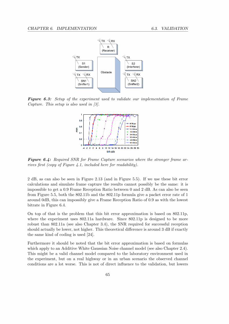
CHAPTER 6. IMPLEMENTATION 6.3. VALIDATION
Figure 6.3: Setup of the experiment used to validate our implementation of FrameCapture. This setup is also used in [3].
Figure 6.4: Required SNR for Frame Capture scenarios where the stronger frame ar-rives first (copy of Figure 4.1, included here for readability).
2 dB, as can also be seen in Figure 2.13 (and in Figure 5.5). If we use these bit errorcalculations and simulate frame capture the results cannot possibly be the same: it isimpossible to get a 0.9 Frame Reception Ratio between 0 and 2 dB. As can also be seenfrom Figure 5.5, both the 802.11b and the 802.11p formula give a packet error rate of 1around 0dB, this can impossibly give a Frame Reception Ratio of 0.9 as with the lowestbitrate in Figure 6.4.
On top of that is the problem that this bit error approximation is based on 802.11p,where the experiment uses 802.11a hardware. Since 802.11p is designed to be morerobust than 802.11a (see also Chapter 3.4), the SNR required for successful receptionshould actually be lower, not higher. This theoretical difference is around 3 dB if exactlythe same kind of coding is used [24].
Furthermore it should be noted that the bit error approximation is based on formulaswhich apply to an Additive White Gaussian Noise channel model (see also Chapter 2.4).This might be a valid channel model compared to the laboratory environment used inthe experiment, but on a real highway or in an urban scenario the observed channelconditions are a lot worse. This is not of direct influence to the validation, but lowers
65

6.3. VALIDATION CHAPTER 6. IMPLEMENTATION
(a) Sender First (b) Sender Last, Interference Clear
(c) Sender Last, Interference Garbled
Figure 6.5: Comparison of the Frame Capture results for different scenarios betweenthe experiments performed in [3] and the estimated results based on our implementation.
its value - due to the nature of the typical vehicular network channel it seems unlikelythat frames can be captured successfully with SNRs between 0 and 2 dB.
The last difficulty in all of this is that there are no known other experiments that wecould use to verify our capture implementation, let alone experiments done with real802.11p hardware. (802.11p hardware, it must be noted, is still quite scarce because ofthe novelty of the new standard). We are thus stuck with a capture experiment witha lot of variables that are different from the simulation environment, but no suitablealternative we can use to validate our implementation.
6.3.3 Expected results
Due to these limitations it is impossible to validate our capture model with hard data -we just have to assume that the capture logic is at least reasonably accurate based onthe results from the experiments. The capture results that we expect with our modelare compared in Figure 6.5.
66

CHAPTER 6. IMPLEMENTATION 6.3. VALIDATION
Please note that because of all the constraints mentioned in this chapter our implemen-tation of frame capture is merely an approximation. The lack of available literatureon this topic has made it a very challenging task to accurately model Frame Capturespecifically for 802.11p. Our approximation should be further verified, preferably byexperiments with real 802.11p hardware.
6.3.4 Results
In spite of all the shortcomings, we have performed simulations that mimic the experi-ment mentioned above, to show that our implementation behaves like we think that itbehaves. We have created a network with three nodes, one receiver and two senders oneither side. If the other sender was silent, the receiver could correctly receive a framefrom either node. We let both nodes generate new beacons using a Poisson process, thenwaiting a quarter of a second (to make sure there would not be three frames associatedwith one capture event but always only 2) and then generating a new beacon again usinga Poisson process. We logged all capture events and classified them accordingly.
In Figure 6.6 the capture results are shown. Because of the implemented capture thresh-olds at 8 and 16 dB, the Frame Reception Ratio jumps to 1 at these thresholds in theSLC and SLG cases; i.e. at the SNR where the capture thresholds are exceeded, thebit error calculation formulas do not have much influence on the results. This is alsoindicative of the shortcomings of the current BER implementation. In a real scenariothese changes are not likely to be that abrupt, although for lower bitrates it is possi-ble. As already mentioned, capture experiments with real 802.11p hardware should beperformed to be able to fine-tune the model reliably.
67

6.3. VALIDATION CHAPTER 6. IMPLEMENTATION
Figure 6.6: Frame Capture simulation results of our validation experiments (all trafficat 3 Mbps). Because of the implemented capture thresholds the reception ratio jumpsfrom 0 to 1 at these thresholds. This will not be the case at the higher bitrates, wherethe required SNR for correct reception is higher than the capture thresholds, not lower.
68

7Simulations
This part of the thesis covers the research questions regarding vehicular networks: howdoes Frame Capture influence IEEE 802.11p network performance? We suspect that inhigh-density traffic scenarios, Frame Capture has a significant effect on throughput in avehicular network if the chipset supports it. If a frame is captured, a collision no longernecessarily means loss of bandwidth. Frame capture always occurs during a collision(i.e. a chipset could then capture a frame in favor of an other, weaker frame), so anyscenario where many collisions occur is interesting for us. A vehicular network is such anenvironment, especially when there are many cars and they all broadcast beacons at arate that is so high that the medium becomes saturated. By doing these simulations wedemonstrate that Frame Capture has a measurable impact on performance in broadcast-oriented vehicular networks, and we show that the expected performance boost can varyamong different chipsets.
We have made two significant changes to the simulator. First, we implemented FrameCapture so that not all frames during a collision are necessarily lost; second, we changedthe bit- & packet error rate calculation formulas so that they better reflect 802.11p.Both these improvements should be considered separately when measuring the influenceof either one; when introducing both changes simultaneously it is very hard to see whichchanges in the results reflect which changes in the implementation.
69

7.1. SIMULATION PLAN CHAPTER 7. SIMULATIONS
7.1 Simulation plan
For our simulation scenarios, the simulation parameters that are considered relevant areshown in Table 7.1. Regarding Frame Capture, we compare three different implementa-tions, one with capture behavior that mimics Atheros chipsets, one that mimics Prismchipsets and one that has no capture behavior at all, i.e. all collisions result in the lossof both frames. We also study the impact of the new bit error approximation formulasto make sure they do not affect capture behavior in the simulator.
Some parameters that are important in a vehicular network have been fixed, i.e. notvaried with different simulation runs. We did this for various reasons; mostly becausechanging these variables would not change the observed capture behavior or because thenumber of simulations that needed to be performed would grow too large. Some of theparameters listed could however have a great impact on the throughput and saturationrate of the medium and should be investigated further in the future.
As can be seen, we simulate that all cars are moving on a line (a highway with 1 or4 lanes). We abstract away the real movement however by assuming that all nodesare moving in the same direction and at a constant speed, which causes the distancesbetween the nodes not to change.
The following sections describe some of the important metrics, and how they will influ-ence the simulation results.
7.1.1 Road vehicle density
The number of nodes (together with the traffic generation rate) is an important metricbecause they have great influence on the number of collisions that are likely to occur ina vehicular network. There are a few different scenarios.
If the distance between nodes (or node density) is approximately equal to the trans-mission range, there is only one hidden terminal for every sender-receiver pair. Thisis shown in Figure 7.1, where the blue node (the Sender node) tries to broadcast aframe. The two green nodes (the Receiver nodes) will receive it because they are in thecommunication range, the two red nodes (the Quiet nodes) will hear the transmissionand can sense that the medium is busy. However the black nodes will not hear thetransmission, and can start sending at any moment, affecting the reception of one of thegreen nodes. In this scenario (where there is one node in the communication range andone in the transmission range, there is exactly one hidden terminal for every ongoingtransmission.
If we double the node density, the number of hidden terminals also doubles (if thedistance between sender and receiver remains the same), as is shown in Figure 7.2. Thisshows that we can easily increase the effects of the hidden terminal problem by graduallyincreasing the node density. The number of hidden terminals in this case also depends
70

CHAPTER 7. SIMULATIONS 7.1. SIMULATION PLAN
Q R S R HQH
H
Figure 7.1: The relationship between the node density and the hidden terminal problemfor a low-density scenario. The blue node (S) transmits a message. The green nodes (R)can receive the message, the red nodes hear the message and will not transmit (Q), theblack nodes (H) cannot hear the message and can thus at any moment start interferingwith the ongoing transmission (i.e. they are hidden terminals).
on which receiver is being considered; a node further away from the sender has morehidden terminals.
Q R S R QQ Q R R Q QH H H H
Figure 7.2: The relationship between high node density and the hidden terminal prob-lem. (S = Sender, R = Receiver, Q = Quiet, H = Hidden)
Please note that these figures are a simplification of reality; under real circumstancesthere is a zone where the correct reception probability decreases gradually instead ofa hard boundary as shown in the figures. Also, the relative size of the nodes to theircommunication range is not to scale.
71

7.2. BASIC PARAMETERS CHAPTER 7. SIMULATIONS
7.1.2 Traffic generation rate
The traffic generation rate is not that important to us, because in the scenarios describedabove where movement between the nodes is abstracted away, an increased traffic gen-eration rate would only create more collisions and capture events of exactly the samekind. If the scenario in the first image would use a traffic generation rate that is twice ashigh as the second image, the number of collisions caused by hidden terminals would bemore or less the same assuming a Poisson process generated the beacons. However, thenumber of collisions because of simultaneously ending backoff counters could be differ-ent; since the contention windows do not scale linearly with either the node density orthe number of collisions the nodes experience. Also, in our scenario where we have onlybroadcast traffic, the contention window does not scale at all, because broadcast trafficnever gives feedback to the MAC layer (in the form of an ACK frame or the lack of it) asan indication that the transmission was lost. To simplify our simulation environment weassume a fixed traffic generation rate of 10 Hz. The relative impact of collisions betweencoordinated nodes vs. collisions caused by the Hidden Terminal Problem is discussed inChapter 7.2.2.
7.1.3 Node chain length
Another important issue is the node chain length, i.e. the number of cars in total onthe highway. We simulate a highway but we wrap around the simulation space in thex dimension, locating the nodes on a ring instead of on a straight line. This causesall the nodes to have the same number of neighbors and all transmissions to have thesame number of hidden terminals and thus, the same collision probability. If we were tosimulate on a straight line, the conditions at the start and the end of the line would bedifferent from the conditions in the middle.
7.2 Basic parameters
The basic parameters of the simulation are described in this section. All nodes havefixed positions on a line and for every node the distance to their nearest neighbor is (intheir lane) always equal. For the single-lane scenario we simulate a stretch of highwayof 2000 m, and vary the number of nodes between 1 and 15 nodes per 100 meters. Themulti-lane scenario is a stretch of 4 lanes, every lane 1000 meters long, and the nodedensity varies here between 0.5 and 15 nodes per 100 meters per lane. This means thatthe total network has between 20 and 300 nodes in the single-lane scenario, and between20 and 600 nodes in the multi-lane scenario.
All nodes broadcast 100 beacons of 3200 bits (≈ 450 bytes with headers) at a rate of10 Hz. The traffic is generated with a Poisson process, meaning that the times between
72

CHAPTER 7. SIMULATIONS 7.2. BASIC PARAMETERS
subsequent transmissions are exponentially distributed with µ = 0, 1. This distributionis used because it also reflects the arrivals of beacons in reality.
The thermal noise is set at -100 dBm. The capture thresholds are implemented asdescribed in Chapter 6 and set at 0, 8 and 16 dB respectively. Radio switching timeshave been omitted, i.e. a receiving radio can switch between sending and receiving modeinstantly. The receiver sensitivity is set at -94 dBm which is a typical value for 802.11chipsets at their lowest bitrate (note that the receiver sensitivity is usually bitrate-dependent). The maximum transmission power of all nodes is 1000 mW, which is equalto 30 dBm, the maximum transmission power under the European regulatory domain[7]. As a comparison: the maximum vehicle transmit power in the United States is 28.8dBm, equal to 750 mW (1028.8/10 = 758 mW) [58].
We use a path loss factor (α) of 3.2, which is typical for a relatively lossy urban en-vironment [38]. While this path loss factor is too high for a typical highway withLOS communication (e.g. if two vehicles have their antennas mounted clearly abovethe vehicle and the antennas radiate in the right direction), we cannot assume that alltransmissions will always have an LOS component. Vehicular networks will operate notonly on highways but also in urban environments, or there could be a big truck posi-tioned between the sender and receiver for example. This path loss factor means thatthe maximum interference distance of a node is 239 meters, as can be seen in Equation7.1 [8, 51].
Di =λ2 · Pt
16π2Pmin
1/α
where
Di = maximum interference distance,
λ = wavelength =c
f2= speed of light / frequency2,
Pt = transmission power (mW)
Pmin = minimum receive power = 10−Rxsens/10
Rxsens = receiver sensitivity (dBm)((2.998 · 108/5.9 · 109)2) · 1000
16 · π2 · 10−9.4
)1/3.2= 239, 46m
This is a reasonable distance to work with, certainly in the scope of vehicular networks.With these parameters, we perform six single-lane simulations that can be seen in Table7.2. Initially we performed each simulation 10 times. Based on these 10 repetitions wecalculated the 95% and 99% confidence intervals, and they appeared to be very wide (seealso 7.4). With this knowledge we finally performed every simulation run 5 times.
73

7.2. BASIC PARAMETERS CHAPTER 7. SIMULATIONS
7.2.1 Multi-lane
After doing the single-lane simulation runs, the results indicated that we did not stretchthe network to the limit from a capacity point of view. In order to put an even biggerload on the network and find out if Frame Capture is even more important if nodes donot just have neighbors in front of and behind them, but also on their sides, we decidedto also perform simulations for a 4-lane highway. Because the simulation time increasesexponentially with a linearly increasing node density, we have reduced the length ofthe highway to 1000 meters for these multi-lane scenarios. The node density per 100meters of highway remains the same, so at the highest node density we simulate with 600nodes. The distances between the nodes in one lane are still equal for every simulationrun, but between lanes there are slight differences; the nodes in every lane are shifteda few meters (one-third of the distance between cars on one single lane) compared tothe previous lane. In the multi-lane scenario we only look at the different behaviorregarding Frame Capture, the bit error calculations can be sufficiently analyzed withjust the single-lane scenario.
7.2.2 Hidden Terminal Problem
As we have concluded in Chapters 3 and 4, Frame Capture is closely related to the hiddenterminal problem. There are two types of collisions that will occur in the network: theones because of the hidden terminal problem (or HTP collisions), and the ones betweencoordinated nodes whose backoff counters end simultaneously (or Coordinated Nodecollisions). We suspect that Frame Capture is more important with HTP collisions thanwith CN collisions, because the observed SNR difference is larger with hidden terminalssimply because the distance between the colliding nodes is larger. As can be seen fromthe capture thresholds, a chipset needs a certain SNR to capture a new frame. What wethus wanted to find out was how many collisions and captures originate from the hiddenterminal problem, and how many originate from the coordinated nodes. To answerthat question, we performed simulations where we ’turned the hidden terminal problemoff’.
If many collisions occur because of hidden terminals, we suspect that Frame Capturecan play an important role in improving the network’s throughput. We can effectivelydisable the hidden terminals by lowering the receiver’s sensitivity threshold, making anode able to hear frames at a larger distance. Note: if the simulation space is flat, andnode A wants to broadcast, he must hear the ongoing transmissions of any other nodeof at least 2 transmission ranges away to disable the hidden terminal problem. This isbecause for any of those transmissions A might be a hidden terminal.
We can achieve this disabling of the hidden terminal problem using the ConnectionMan-ager of OMNeT++. By lowering the signal attenuation threshold we can connect thenodes that are normally outside of the node’s transmission range. All parameters thatwere mentioned before are still the same, but we added one more sensitivity threshold,
74

CHAPTER 7. SIMULATIONS 7.3. METRICS
the HTP sensitivity. If a frame’s power level is above this threshold, the receiver stillmarks the medium as busy, even though it is unable to receive the frame and outsideof the transmission range of the sending node. We lowered this threshold to -105 dBm.If we input this new signal attenuation threshold in Equation 7.1, we see that the Con-nectionManager will connect all nodes up to around 528,42 meters away. By setting theHTP sensitivity threshold to -105 dBm as well, we silenced all hidden terminals up tothat distance (which is around 2 transmission ranges).
The only collisions that will still occur in this new scenario are the collisions betweencoordinated nodes. The difference in throughput measured and the collision probabilityof these new scenarios give us an indication of how many HTP collisions normally occurin the network. If the collision probability is a lot lower than in the normal scenarios,we know that the impact of the hidden terminal problem is normally very large.
Table 7.2 gives an overview of all the different simulations we performed, with the differ-ent capture behaviors and the different bit error rate calculation implementations. The802.11b implementation is the current one, the 802.11p implementation is our modifiedimplementation. The numbers in the table cells indicate the number of repetitions foreach simulation. Note that the number of repetitions is not an important metric onitself, it is merely an indication and it is used to calculate the confidence intervals of thecalculated metrics.
7.3 Metrics
During the simulation runs the collection of the right metrics is essential to give usinsight in the performance of the network. OMNeT++ already has modules dedicated tometrics collection. From within any OMNeT++ module the function recordScalar(name,value) can be called, storing a name-value pair. These name-value pairs can be storedin plain text files, or in any other way that the user wants. We set up a MySQLdatabase that recorded all the relevant scalars after every simulation run. Note that thisoccurred on a per-node basis, so aggregation of information was necessary after runningthe simulations.
Apart from the general network performance metrics, we also wanted to have moreinformation on the capture events that took place. Therefore we also recorded a fewmetrics for every capture event that took place (e.g. whether the capture event wassuccessful, what the observed SNR was, what the arrival time difference was etc. )
Both the capture metrics and the metrics we needed to provide us insight in the perfor-mance of the network are listed in Table 7.3.
Note that if multiple frames arrive during the reception of a frame, the mentionedarrival time difference and other frame state both apply to the first other frame thatwas involved in a capture event. For example if a strong frame B arrives during the
75

7.3. METRICS CHAPTER 7. SIMULATIONS
reception of a weaker frame A and the receiver captures frame B, and then duringreception of B weaker frames C and D arrive at the receiver (in both cases the receiverstays locked to frame B). The number of capture events is 3 (A&B => B, B&C => B,B&D => B) and the capture count is 4 because there were 4 frames involved. However,the recorded arrival time difference and other frame state apply to A and B only. TheSNR difference applies to all frames (A, C and D are summed as interference).
Not every single one of these metrics will be put to use directly and some metrics wereonly used for validation purposes, but the possibility exists that based on the resultswe want to zoom in on a certain part of Frame Capture; the broad metrics collectiondescribed here provides us the means to do so if necessary.
76
CHAPTER 7. SIMULATIONS 7.3. METRICS
From these basic counters we can calculate the more advanced metrics which providereal insight in the network performance:
• beacon success probability - this is the percentage of the frames that are receivedcorrectly that also could have been received correctly. If a node broadcasts a beaconto 10 other nodes (all within communication range) and 9 receive it correctly, thebeacon success probability is 90%. This percentage can be calculated by dividing,for every node, the number of successfully received frames by the number of framesthat it could lock onto (i.e. frames arriving that were stronger than the receiversensitivity). Since the throughput is hard to visualize in a broadcast network, thisis our most important metric. The throughput in bytes/second doesn’t say muchin a network with only broadcast traffic, because for every transmission there isone sender and many receivers. This gives a distorted image of the capacity of themedium.
• capture factor - # successful captures / # frames received correctly - this tells ushow many frames are received thanks to Frame Capture, i.e. how big the influenceof Frame Capture is on the total reception process.
• capture success probability - # successful captures / # capture events - this tellsus what the average probability of success is when a capture event takes place.
• collision probability - # collisions / # arriving frames (above sensitivity threshold)- the collision probability is a good indication of the load on the network and theprobability of suffering from interfering frames during a transmission.
We can then visualize, for different node densities, what the impact of Frame Captureis on a vehicular network with the (aggregated) metrics described above.
77

7.4. RESULTS CHAPTER 7. SIMULATIONS
7.4 Results
This section discusses the results of all the simulations that we performed. Note that innone of the graphs the confidence interval of the graphs is visualized. This is because thecalculated confidence intervals (calculated with the t-distribution), even at 99%, wereso small that they were not worth plotting. They were usually less than 0,2% for thevarious aggregated metrics.
7.4.1 Single Lane
In the single lane simulations, we compare the three different capture modes and the802.11p and 802.11b bit error calculation implementations. In Figure 7.4 the most im-portant metric is shown as a function of the node density: the beacon success probability(BSP). Remember that we defined the beacon success probability as the percentage offrames that have been received correctly, as compared to the total number of framesthat could have been received correctly, i.e. that were strong enough to be decoded hadthere been no interference.
First, we show the collision probability for all single lane scenarios in Figure 7.3. Sinceall nodes generate traffic at the same rate and the node placement is the same for allscenarios, the collision probability is also the same. This gives us an indication of theload of the medium.
0
0.1
0.2
0.3
0.4
0.5
0.6
0.7
0.8
0.9
1
1 2 3 4 5 6 7 8 9 10 11 12 13 14 15
Col
lisio
n pr
obab
ility
(%
)
Road vehicle density (# cars / 100m)
Single Lane - Collision Probability
Collision Probability
Figure 7.3: Collision probability for single-lane scenarios
The collision probability rises steadily when the node density increases, which is asexpected because with increasing node density there are more hidden terminals. Also,since the contention window does not scale with the node density in a broadcast-only
78

CHAPTER 7. SIMULATIONS 7.4. RESULTS
network, the probability of collisions between coordinated nodes (i.e. because theirbackoff timers end simultaneously) also increases. It is not possible to see from thisFigure how the collisions are distributed among these two collision types, we will try toanswer that with the hidden terminal simulations.
If we then look at the BSP for the various scenarios shown in Figure 7.4, we see whatwe expected. In the figure there are three sets of lines; red, blue and green. Each colorrepresents one of the frame capture varieties as displayed in the legend. It is logicalthat for all simulations the BSP decreases when the node density increases, but bothimplementations that are able to capture frames show a higher BSP, indicating theincrease in performance. Note that Atheros performs better than Prism because of itsability to capture a stronger frame even while the receiver is locked to a weaker one.Compared to a chipset that performs no Frame Capture at all, both Atheros and Prismchipsets show a performance boost of at least 20%. The difference between Atheros andPrism are not spectacular but nonetheless noticeable; around 4% for the highest vehicledensity. This BSP however has no one-on-one relationship to the degree of disseminationof information at higher layers (i.e. to what degree all nodes receive the information thatis relevant to them). Depending on the application level protocol, a BSP of 50% canstill be sufficient to meet the application requirements.
Figure 7.4: Beacon success probability (BSP) comparison for the single lane scenariosbetween the three capture modes and both bit error calculation approximations.
The dashed lines show the BSP when the 802.11b BER calculations are used, comparedto the solid lines which show the BSP with 802.11p. It appears that 802.11b ’performs’ a
79

7.4. RESULTS CHAPTER 7. SIMULATIONS
bit better and this can be directly explained through Figure 5.5 - at SNR values approx-imately between 1 and 3 dB the 802.11b-specific formulas predict an almost negligiblepacket loss, whereas the new formulas still predict that a substantial part if not all ofthe frames are lost. Note that this is not really a performance gain because the 802.11bformulas simply do not apply to the physical layer in an 802.11p-based vehicular net-work. This merely shows that the implementation of the new BER and PER formulasdoes not affect the expected behavior regarding Frame Capture. The approximation for802.11p is certainly closer to a real vehicular network than its 802.11b counterpart, butwe suspect that when all channel effects are considered, the resulting approximation iseven more pessimistic, and thus the BSP even lower.
If studied closely, it can be seen that for the implementation without Frame Capturethe 802.11p and 802.11b BSP is almost the same for all node densities. The fact thatthis implementation shows no difference between 802.11p and 802.11b can be easilyunderstood. From the literature in Chapter 4.2 and general literature on wireless com-munications we concluded that the preamble of a frame is the most important phaseto ensure correct reception. The signal-to-noise ratio that a receiver needs to lock to aframe is above the range where the differences between 802.11p and 802.11b manifest,and this implementation discards all collided frames. We have double-checked this withour implementation, and all frames that are being processed by the receiver that didnot suffer from interference (either by hidden terminals or by a simultaneously endingbackoff counter) have a signal to noise ratio of around 6 dB. Around 6 dB packet errorrates in both formulas from Figure 5.5 are negligible.
The difference between the two capture implementations (Atheros and Prism) is notvery large - only a few percent. We can further visualize the impact of Frame Capturewith Figure 7.5. This shows, as can also be more or less deduced from the BSP increasein Figure 7.4, that the influence of Frame Capture increases steadily with the increasein node density.
Another observation from this graph (and even more clearly in Figure 7.10 where wediscuss the simulations without hidden terminals) is that the results are a bit ’wobbly’.This is probably caused by a slight methodical error in the approach w.r.t. the granu-larity of the node density we use and the deterministic node placement. Every node isplaced at exactly the same distance to its neighbors. This causes some scenarios whichhave nodes at the borders of the transmission- and interference ranges to behave a bitdifferent. We could mitigate this by placing the nodes not deterministically but using asort of ’jittered’ node placement, where we use a uniform distribution to shift the nodesa little bit to the right or to the left compared to their (current) deterministic placement.However, we would have needed to perform more simulations then to achieve the sameconfidence intervals.
To conclude; in these single-lane scenarios there is definitely a gain in BSP thanks to thecapture behavior in some chipsets. The difference between Atheros and Prism chipsetsis not spectacular, but still measurable, up to 8%. It will be interesting to see if the
80

CHAPTER 7. SIMULATIONS 7.4. RESULTS
0
0.1
0.2
1 2 3 4 5 6 7 8 9 10 11 12 13 14 15
Cap
ture
Fac
tor
Road vehicle density (# cars / 100m)
Single Lane - Capture Factor
Capture Factor - AtherosCapture Factor - Prism
Figure 7.5: The Capture Factor is the percentage of successfully received frames thanksto Frame Capture.
impact of Frame Capture becomes even larger in a scenario with an even higher nodedensity, such as our multi-lane scenario.
81

7.4. RESULTS CHAPTER 7. SIMULATIONS
7.4.2 Multi Lane
In the multi-lane scenario, the number of hidden terminals is approximately 4 timeshigher than in the single-lane scenario. Linear increase in the number of hidden terminalsmeans that the hidden terminal collision probability will also increase linearly, becausehidden terminals are not synchronized to the transmitting node. The probability ofcollision between coordinated nodes will also increase linearly for a while, until themedium saturates. The medium is saturated if every node always has a packet waitingfor transmission and all nodes are contending for the medium. In our simulation scenariosthe contention window size never changes, because at the MAC layer there is no recoveryor contention window adaptation because of ’lost’ broadcast frames (a broadcast framecan lost at one node but received correctly at another). We visualize this with Figure7.6; we have added the collision probability for the single-lane scenario for readabilitypurposes. One would expect that when the contention window size doubles for everycollision that is detected, the collision probability would not increase linearly in verydense networks. However because the contention window is fixed, it can be seen thatin our case the collision probability does exactly that. For most node densities it isapproximately 4 times higher and increases linearly until 10 nodes per 100 meter perlane. Beyond that point it flats out a little bit as the medium saturates. This flatteningmight be caused by dropping frames from the queue at the MAC layer, but we did notinclude a metric for that so with the simulation runs that we performed we cannot besure that that is the case.
0
0.1
0.2
0.3
0.4
0.5
0.6
0.7
0.8
0.9
1
0 1 2 3 4 5 6 7 8 9 10 11 12 13 14 15
Col
lisio
n pr
obab
ility
Road vehicle density (# cars / 100m / lane)
Multi Lane - Collision Probability
Multi Lane (4 lanes)Single Lane (1 lane)
Figure 7.6: Collision probability for single- and multi-lane (4 lanes) scenarios
82

CHAPTER 7. SIMULATIONS 7.4. RESULTS
0
0.1
0.2
0.3
0.4
0.5
0.6
0.7
0.8
0.9
1
0 1 2 3 4 5 6 7 8 9 10 11 12 13 14 15
Bea
con
Suc
cess
Pro
babi
lity
Road vehicle density (# cars / 100m / lane)
Frame Capture - Multi Lane
AtherosPrism
No Capture
Figure 7.7: Beacon success probability comparison for the multi lane scenarios, all with802.11p bit error calculations.
The BSP for the multi-lane scenarios is also very interesting to look at, it is shown inFigure 7.7. The figure shows that the BSP decreases rapidly with increasing node density,but also that Frame Capture plays an important role in mitigating that BSP decrease.There appears to be an optimum where the performance gain is the largest, around 7nodes per 100m per lane. In all cases Atheros again slightly outperforms Prism. Asthe node density increases further it appears that the medium becomes saturated andthe MAC layer starts to drop frames at the queue, causing the BSP to decrease lessdramatically and more or less stabilize around 0.1.
The capture factor shown in Figure 7.8 shows the same image. Up to a node densityof around 10 vehicles per 100m per lane the capture factor grows linearly with nodedensity, but then the medium saturates and the capture factor stabilizes, or even appearsto decrease slightly.
Obviously the increased number of neighbors every node has causes the number of colli-sions to increase rapidly and the BSP to decrease rapidly as well. This effect is amplifiedby the fact that all nodes have a fixed contention window. It would be interestingo compare the network performance with unicast networks (which use RTS/CTS andhave fewer hidden terminals), and to vary the contention window size to see if FrameCapture remains equally important with a different contention window.
Since the transmissions from a node that is close by and a hidden terminal are likely
83

7.4. RESULTS CHAPTER 7. SIMULATIONS
0
0.1
0.2
0.3
0.4
0.5
0 1 2 3 4 5 6 7 8 9 10 11 12 13 14 15
Cap
ture
Fac
tor
Road vehicle density (# cars / 100m / lane)
Multi Lane - Capture Factor
AtherosPrism
Figure 7.8: Capture Factor for the multi-lane scenarios.
to have significant difference in power levels, the probability that the strongest framecan be captured in a hidden terminal collision is higher than with collisions betweencoordinated nodes. And because the hidden terminal problem occurs less in unicastnetworks, there are probably fewer capture events in such a network. We can concludethough that for broadcast networks, Frame Capture definitely has a positive impact onperformance.
84

CHAPTER 7. SIMULATIONS 7.4. RESULTS
7.4.3 Hidden Terminal Problem
In this section we describe the results from our simulations where we eliminated theHidden Terminal Problem. We simulated both a single-lane scenario and a multi-lanescenario (with the Atheros chipset behavior and the 802.11p bit error approximations).The node placement, number of lanes and all other physical layer parameters are equalto the regular simulations, only the hidden terminals are silenced. The results are shownin the figures below.
The first graph (Figure 7.9) shows the collision probability for both the single- andthe multilane scenarios. In both cases the collision probability is at least 50% smallercompared to the normal scenario (at the higher node densities). This also shows therelative impact of the hidden terminal problem - all collisions in the scenario withouthidden terminals (the dashed lines) are caused by simultaneously ending backoff coun-ters. Therefore the difference between the dashed and the colored lines of each color inFigure 7.9 demonstrates the relative contribution of the hidden terminal problem andthe backoff counters to the total number of collisions. It can be seen that for both sce-narios at least 50% of all collisions can be attributed to the hidden terminal problem.The numerical results (not shown) indicate that at 15 cars per 100 meters (per lane)the exact percentages of HTP collisions are 58,4% (single-lane) and 53,5% (multi-lane)respectively.
The reason that the percentage of HTP collisions in the multi-lane scenario is a bit loweris because of the combination of the fixed contention window size and the increased nodedensity. Having more coordinated nodes with the same contention window size meansthat the probability of a coordinated node collision increases (that can be concludedfrom comparing the two dashed lines).
What is even more interesting is that this increase in node coordination actually de-creases the beacon success probability for the multi-lane scenario. This can be seen inFigure 7.10. The single-lane scenario is not very surprising; because the medium is notsaturated, the absence of hidden terminals increases the beacon success probability alittle bit. However in the multi-lane scenario, where the medium does become saturated,the increased node coordination has actually negative effects. With our simulation, allnodes in the multi-lane scenario are coordinated, because the HTP sensitivity thresholdcauses nodes to indicate that their channel is busy up to 530 meters away, and the stretchof highway is 1000 meters. This has two effects:
• there is only 1 ongoing transmission in the medium at the same time; only ifrandom backoff timers end simultaneously there are more than 1).
• nodes have to wait longer on average before they observe the medium as ’idle’. Be-cause of this the buffer occupancy at the MAC layer is higher on average, meaningthat more nodes have a beacon waiting for transmission. Unfortunately we hadno instrumentation in place to measure this, so this could not be confirmed withhard evidence.
85

7.4. RESULTS CHAPTER 7. SIMULATIONS
0
0.1
0.2
0.3
0.4
0.5
0.6
0.7
0.8
0.9
1
1 2 3 4 5 6 7 8 9 10 11 12 13 14 15
Col
lisio
n pr
obab
ility
Road vehicle density (# cars / 100m)
Hidden Terminal Problem - Collision Probability
Normal - Multi LaneWithout HTP - Multi Lane
Normal - Single LaneWithout HTP - Single Lane
Figure 7.9: Collision probability in the scenarios without hidden terminals.The uppertwo lines belong to the multi-lane scenario.
Now if all nodes (including the hidden terminals) freeze their backoff timers when atransmission is ongoing somewhere in the network, and all nodes always have a trans-mission ready as soon as they sense the medium has become idle again, there are a lotof collisions between coordinated nodes. And these are exactly the type of collisionsthat are hard for Frame Capture to ’correct’, because coordinated nodes usually have amore-or-less equal signal strength; the fact that they are coordinated indicates that thedistance between them is smaller on average.
The changes to the scenarios mentioned above (silencing the hidden terminals and artifi-cially making all nodes coordinated) have a strange effect: in our case, with a fixed con-tention window, the beacon success probability actually decreases instead of increases.Even though the probability of a collision is lower (the total number of collisions is ofcourse also lower), a very large percentage of collisions that do occur cannot be miti-gated by Frame Capture. This is also shown in Figure 7.11, where the Capture Factor inthe multi-lane scenario without hidden terminal stalls very quickly and even decreases alittle bit. This shows very clearly that Frame Capture is especially useful when resolvingcollisions caused by hidden terminals and that ’disabling’ hidden terminals (and thusintroducing node coordination where it is not necessary) will not solve the problem. Howthis manifests with different contention window sizes could be an interesting questionfor further study.
86

CHAPTER 7. SIMULATIONS 7.4. RESULTS
0.1
0.2
0.3
0.4
0.5
0.6
0.7
0.8
0.9
1
1 2 3 4 5 6 7 8 9 10 11 12 13 14 15
Bea
con
Suc
cess
Pro
babi
lity
Road vehicle density (# cars / 100m)
Hidden Terminal Problem - Beacon Success Probability
Normal - Single LaneWithout HTP - Single Lane
Normal - Multi LaneWithout HTP - Multi Lane
Figure 7.10: Beacon success probability in the scenario without hidden terminal colli-sions. The upper two lines belong to the single-lane scenarios.
The reason that we do not see this behavior in the single-lane scenario is that we donot enter the same ’collision regime’ there. The single-lane highway is 2000 meters longinstead of 1000 meters, meaning that not all nodes are coordinated. Basically what wesee in every graph regarding the single lane metrics (the red lines) only represents thefirst part of the multi-lane scenarios, where the medium is not saturated yet and not allMAC queues are constantly occupied.
87

7.4. RESULTS CHAPTER 7. SIMULATIONS
0
0.1
0.2
0.3
0.4
0.5
1 2 3 4 5 6 7 8 9 10 11 12 13 14 15
Cap
ture
Fac
tor
Road vehicle density (# cars / 100m)
Hidden Terminal Problem - Capture Factor
Normal - Single LaneWithout HTP - Single Lane
Normal - Multi LaneWithout HTP - Multi Lane
Figure 7.11: Comparison of the Capture Factor in the normal scenario and withouthidden terminal collisions. The upper two lines belong to the multi-lane scenarios.
88

CHAPTER 7. SIMULATIONS 7.4. RESULTS
Table 7.1: Frame Capture simulation scenarios
Variable Explanation
Frame Capture We use three different Frame Capture imple-mentations: One representing the Atheros be-havior, one for Prism, and one which has nocapture at all. This last implementation is notbased on a real chipset but used as a reference tomeasure the performance boost caused by FrameCapture.
Bit Error Calculations We use two implementations: the one based on802.11b (current implementation), and our mod-ified implemenation based on 802.11p.
Road vehicle density We vary the road density between 1 and 15 carsper 100 meters in steps of 1 (single-lane) or 0.5(multi-lane). One car per 100 meters is equal tovery little traffic, and 15 cars per 100 meters is(roughly) equal to bumper-to-bumper.
Vehicle placement This is not varied, the vehicle placement is de-terministic. Nodes are placed at equal distancesfrom each other.
Network traffic genera-tion
Beacon generation is Poisson-based with fixed µ(=0,1). This is equal to 10 beacons per secondon average.
Movement We assume constant (and equal) speed for allvehicles.
Highway width We use two different values here: we simulatea single-lane highway with only 1 lane, and amulti-lane highway with 4 lanes.
Beacon length We use a fixed beacon length of 3200 bitsData rate The data rate we used is 3 Mbps in all cases.
Table 7.2: Simulation scenarios (numbers indicate # repetitions)
Single-Lane Multi-Lane w/o HTP
SL ML
802.11p 802.11b 802.11p 802.11p 802.11p
Atheros 5 5 3 5 3
Prism 5 5 3 - -
No Capture 5 5 3 - -
89

7.4. RESULTS CHAPTER 7. SIMULATIONS
Table 7.3: Simulation metrics
Metric Details Scope
# frames sent node
# framesreceivedcorrectly
The number of frames that were received and were strongenough to be decoded correctly.
node
# framesreceived
This is the number of frames that the ConnectionManagerdelivered at the node’s input gate (see also Chapter 5). Thisis not the number of correctly received frames!
node
# strong framesThe number of frames that arrived with a signal strengthabove the receiver sensitivity.
node
# frames lockedThe number of frames that the receiver actually lockedonto.
node
# collisionsThe number of frames arriving when the receiver is alreadyreceiving an other frame.
node
# captureevents
The number of times that the receiver captures a frameduring a collision. This happens when, after the preambleof the colliding frame, the receiver is (still) locked on to aframe, either the new one or the old one. If the receiver wasnot locked to the old frame and the new frame is not strongenough (i.e. is not above the capture threshold), there isno capture event.
node
# successfulcaptures
The number of times that a frame is captured and after thatframe ends it is received correctly. Note that capturing aframe does not guarantee successful reception. Figure 6.6seems to indicate that is the case, however that is only truefor the lower bitrates. Also, if a lot of weak interferencearrives after the preamble, the overall SNR will also beinsufficient for correct reception.
node
arrival timedifference
The difference in arrival time between two colliding framesinvolved in a capture event.
captureevent
SNR differenceThe signal to noise ratio of the frame that the receiver locksonto after the capture event.
captureevent
capture countThe number of frames that arrived at the receiver duringthe entire reception of the captured frame.
captureevent
capture resultWhether the captured frame was decoded correctly after itsreception or not.
captureevent
other framestate
What the state of the other (lost) frame was when the re-ceiver captured the frame.
captureevent
90

8Conclusions
In this thesis, we investigated Frame Capture. All aspects of the phenomenon cameto light, thanks to the available literature and the simulations we performed with ourenhanced physical layer implementation.
As it appeared, there is no single Frame Capture implementation. The exact behavior isdifferent among chipsets from various manufacturers [5, 15, 6, 3, 47]. We looked at thebehavior in Atheros and Prism chipsets in particular, thanks to the available literaturefrom the academic field on those two chipsets. Whether a receiver is able to capture aframe depends also on the signal-to-noise ratio, whether the frame receives interferenceduring the preamble or not, and the difference in arrival times between the two collidingframes. However if a frame is captured, the literature indicates that this is always thestrongest frame. Prism chipsets [59] can capture a stronger frame during a collisiononly if the stronger frame arrives first or during the preamble of the weaker frame. Thebehavior from Atheros chipsets [46] is slightly better from a performance point of view,because it is able to capture a frame independent of the state of the other frame. Theexact workings of Frame Capture at a circuit level are hard to figure out; device & chipsetmanufacturers do not share their circuit designs unfortunately. This makes it harder todeduce the exact capture behavior, since it can only be observed through experiments,not by analyzing the design of the hardware itself.
We modeled the behavior of Frame Capture with so-called capture thresholds, which areSNR thresholds that the frame must exceed before the receiver is able to capture it.Depending on the state of the current frame, a different threshold is used to capture anew frame. If the receiver is still locked to the weaker frame, the new frame must beat least 8 dB stronger. However if the receiver is not locked to the weaker frame the
91

CHAPTER 8. CONCLUSIONS
required SNR threshold is higher as well, because the noise becomes ’uncorrelated’ andthe receiver has more trouble suppressing it. In those cases we use a threshold of 16 dB.If there is no interference at all, the SNR must be at least 0 dB (i.e. stronger than thethermal noise).
We enhanced the current MiXiM physical layer implementation to enable frame captureusing the thresholds described above. MiXiM previously (and by accident) only sup-ported a part of the Prism-like capture behavior; it could only receive stronger framesif they arrived earlier, not during the preamble. During the performed simulations withFrame Capture it became clear that both Prism and Atheros chipsets perform at least20% better than a chipset without any form of Frame Capture. Atheros performed anadditional 5 to 8% better compared to Prism. We have also improved the bit-errorcalculation formulas that are used to determine or predict correct frame reception. Thecurrent implementation was based on IEEE 802.11b. The difference between both imple-mentations is not spectacular, and the formulas are still not ideal because they assumeAdditive White Gaussian Noise as the only interference, but with their implementationwe make a step forward towards better 802.11p channel modeling.
Apart from the normal simulations we also tested the importance of Frame Capturein combination with the hidden terminal problem. We did this by artificially disablingall nodes in the hidden terminal range. We increased the carrier sensing sensitivityso that nodes which would normally be hidden, would now be aware of the ongoingtransmission and set their channel to busy, refraining from sending until the transmissionwas over. What we found there was really interesting; the remainder of collisions (thatwas caused by coordinated nodes) could usually not be resolved by Frame Capture,because coordinated nodes are usually closer to each other and their signal strengthsdiffer less. This shows that in a broadcast network where nodes use a fixed contentionwindow size, Frame Capture plays a vital role in resolving especially the hidden terminalcollisions - the coordinated node collisions also occur, but the probability that FrameCapture can help in resolving those collisions is a lot smaller. This effectively shows theimportance of Frame Capture in any scenario with lots of hidden terminals, whether itbe a vehicular network or another type of network.
92

9Future work
The impact and importance of Frame Capture in a vehicular network has been proven,but there are still many issues related to Frame Capture that could be studied fur-ther.
First of all, the number of experiments that we based our model on is a bit weak. MoreFrame Capture experiments, especially ones performed with 802.11p hardware, couldhelp a lot in validating the model and further refining it. We have implemented FrameCapture now with hard thresholds that must be exceeded. Perhaps research that isoriented towards electrical engineering and signal theory could provide more insight inhow a chipset uses the PLCP preamble to lock to a frame and under which circumstances.This knowledge could be used to refine our capture model.
It would also be interesting to investigate the impact of Frame Capture in other scenariosand with other physical layers, such as wireless sensor networks (where battery life is animportant issue), and with vehicular networks that use mostly unicast traffic.
The channel model in the simulator could also be improved. Complicated channel effectssuch as multipath fading, scattering and narrowband interference are not yet incorpo-rated in any way, mostly due to their complexity. There are however some modelsavailable, research to find out which one is most suited to a vehicular environment couldbe performed. Perhaps a good channel model could be the two-ray path loss model,which assumes an LOS component of the signal, and a reflection of the signal on theground.
For Frame Capture in particular, the movement between nodes is not very relevant, thatis why we chose to simulate without node movement. A good addition to the simulation
93
CHAPTER 9. FUTURE WORK
space could be to include not only movement in general, but also movement patternsfrom real drivers to the simulation. Part of this work is currently being done by ourresearch group.
Other interesting directions in general for the physical layers of vehicular networks arenot specific to 802.11p. Perhaps the usage of a physical layer with (Wideband) CodeDivision Multiple Access ((W)CDMA) is a very good alternative to OFDM - in WCDMAcollisions are automatically resolved (because every node has its own code) and thesystem degrades gracefully [60]. Also, Multiple-Input, Multiple-Output (MIMO) couldbe investigated to increase channel capacity and scalability which might be needed forcertain types of applications. Another application-dependent useful feature might be toinvestigate the usage of two directional antennas at the front and at the back of eachvehicle, increasing the range of communication in one specific direction. There are manyapplications where a message (e.g. a warning message of an accident) should principallytravel backwards, not forwards.
94

Bibliography
[1] Matthew S. Gast, 802.11 Wireless Networks, O’Reilly, 2nd edition, 2008.
[2] Marc Torrent Moreno, Inter-vehicle communications: achieving safety in a dis-tributed wireless environment, PhD thesis, Universitat Karlsruhe, 2007.
[3] Jeongkeun Lee, Wonho Kim, Sung-Ju Lee, Daehyung Jo, Jiho Ryu, TaekyoungKwon, and Yanghee Choi, “An experimental study on the capture effect in 802.11anetworks”, in WinTech, 2007.
[4] Ministerie van Verkeer en Waterstaat, Kennisinstituut voor Mobiliteitsbeleid, “Mo-biliteitsbalans 2009”, http://www.verkeerenwaterstaat.nl/kennisplein/3/8/
387913/Mobiliteitsbalans_2009.pdf, June 2009.
[5] Jeongkeun Lee, Jiho Ryu, Sung-Jun Lee, and Taekyoung Kwon, “Simulating the802.11a PHY model: how to make it accurate”, ACM, 2008.
[6] Hoon Chang, Vishal Misra, and Dan Rubenstein, “A general model and analysis ofphysical layer capture in 802.11 networks”, in IEEE Infocom Proceedings, 2006.
[7] Institute of Electrical and Electronics Engineers (IEEE), “IEEE Standard for Infor-mation Technology - Part 11: Wireless LAN Medium Access Control (MAC) andPhysical Layer (PHY) specifications - Amendment 7: Wireless Access in VehicularEnvironments”, July 2010.
[8] A. Kopke, M. Swigulski, K. Wessel, D. Willkomm, P.T. Klein Haneveld, T.E.V.Parker, O.W. Visser, H.S. Lichte, and S. Valentin, “Simulating wireless and mobilenetworks in OMNeT++: The MiXiM vision”, 2008.
[9] “OMNeT++: An extensible, modular, component-based C++ simulation libraryand framework”, http://www.omnetpp.org.
[10] Karl Wessel, Michael Swigulski, Andreas Kopke, and Daniel Wilkomm, “MiXiM -The Physical Layer - An Architecture Overview”, in Proceeding of the 2nd Inter-national Workshop on OMNeT++, March 2009.
[11] “IEEE Standard for Information Technology-Telecommunications and InformationExchange Between Systems-Local and Metropolitan Area Networks-Specific Re-quirements - Part 11: Wireless LAN Medium Access Control (MAC) and Physical
95

BIBLIOGRAPHY BIBLIOGRAPHY
Layer (PHY) Specifications”, IEEE Standard 802.11-2007 (Revision of IEEE Stan-dard 802.11-1999), pp. C1 –1184, 12 2007.
[12] Daniel Minoli, Hotspot Networks: Wi-Fi for Public Access Locations, McGraw-HillProfessional, 2002.
[13] Gaddi Blumrosen, “The future of WiMAX”, http://www.thefutureofthings.
com/articles/6361/the-future-of-wimax.html, February 2009.
[14] Wayne Tomasi, Electronic Communications Systems: fundamentals through ad-vanced, Prentice Hall, 5th edition, 2004.
[15] Jeongkeun Lee, Jiho Ryu, Sung-Ju Lee, and Taekyoung Kwon, “Improved modelingof IEEE 802.11a PHY through fine-grained measurements”, Computer Networks,2009.
[16] Vocal Technologies Ltd., “White paper - 802.11a wireless lan”, http://www.vocal.com/redirect/802_11a.html, 2011 May.
[17] Charan Langton, “Coding and decoding with convolutional codes”, http:
//complextoreal.com/chapters/convo.pdf.
[18] Christoph Sonntag, “Orthogonal frequency division multiplexing (OFDM) imple-mentation as part of a software defined radio (SDR) environment”, Master’s thesis,University of Stellenbosch, 2005.
[19] Steve Halford and Karen Halford, “OFDM Architecture and Design Challenges”,http://www.commsdesign.com, May 2002.
[20] Yunpeng Zang, Lothar Stibor, Georgios Orfanos, Shumin Guo, and Hans-JurgenReumerman, “An error model for inter-vehicle communications in highway scenariosat 5.9ghz”, ACM, October 2005.
[21] H. S. Wilf, Combinatorial Algorithms: An Update, Society for Industrial andApplied Mathematics, 1989.
[22] Veronika Shivaldova, “Implementation of IEEE 802.11p physical layer model inSIMULINK”, Master’s thesis, Technischen Universitat Wien, Fakultat fur Elek-trotechnik und Informationstechnik, June 2010.
[23] George C. Clark Jr. and J. Bibb Cain, Error-Correction Coding for Digital Com-munications, Plenum Press, 1981.
[24] John G. Proakis, Digital Communications, 4th edition, 1983.
[25] M. Pursley and D. Taipale, “Error probabilities for spread-spectrum packet radiowith convolutional codes and viterbi decoding”, Communications, IEEE Transac-tions on, vol. 35, no. 1, pp. 1 – 12, January 1987.
[26] Michele Weigle, “Introduction to vehicular networks”, http://www.csl.mtu.edu/cs5461/www/Slide/1-Intro-VANET.pdf, 2007.
96

BIBLIOGRAPHY BIBLIOGRAPHY
[27] Qing Xu, K. Hedrick, R. Sengupta, and J. Vanderwerf, “Effects of vehicle-vehicle/roadside-vehicle communication on adaptive cruise controlled highway sys-tems”, in Proceedings from Vehicular Technology Conference, 2002, pp. 1249–1253.
[28] Jan Rouwendal, “Driver behavior and congestion on highways”, Ersa conferencepapers, European Regional Science Association, 1998.
[29] Atulya Mahajan, Niranjan Potnis, Kartik Gopalan, and An-I A. Wang, “Urbanmobility models for VANETs”, in International Workshop on Next GenerationWireless Networks, 2006.
[30] Marco Fiore, “Vehicular mobility models”, in Vehicular Networks, Stephan Olariuand Michele C. Weigle, Eds., chapter 12. Chapman & Hall/CRC, 2009.
[31] David Murray, Michael Dixon, and Terry Koziniec, “Scanning delays in 802.11networks”, in NGMAST ’07: Proceedings of the The 2007 International Conferenceon Next Generation Mobile Applications, Services and Technologies, Washington,DC, USA, 2007, pp. 255–260, IEEE Computer Society.
[32] Ian Tan, Wanbin Tang, Ken Laberteaux, and Ahmad Bahai, “Measurement andanalysis of wireless channel impairments in DSRC vehicular communications”, inIEEE International Conference on Communications, 2008.
[33] Patrick Robertson and Stefan Kaiser, “The effects of Doppler spreads in OFDM(A)mobile radio systems”, 1999, vol. 1, pp. 329 –333 vol.1.
[34] European Conference of Postal and Telecommunications Administrations,“CEPT/ECC decision of on the harmonised use of the 5875-5925 MHz frequencyband for Intelligent Transport Systems (ITS)”, http://www.erodocdb.dk/Docs/
doc98/official/pdf/ECCDEC0801.PDF, March 2008.
[35] “COMeSafety: Communications for eSafety”, http://www.comesafety.org.
[36] Lothar Stibor, Yunpeng Zang, and Hans-Jurgen Reumerman, “Neighborhood eval-uation of vehicular ad-hoc networks using 802.11p”, in 13th European WirelessConference, 2007.
[37] Jijun Yin, Tamer ElBatt, Gavin Yeung, Bo Ryu, Stephen Habermas, HariharanKrishnan, and Timothy Talty, “Performance evaluation of safety applications overdsrc vehicular ad hoc networks”, in Proceedings of the 1st ACM internationalworkshop on Vehicular ad hoc networks. 2004, VANET ’04, pp. 1–9, ACM.
[38] Theodore Rappaport, Wireless Communications: Principles and Practice, PrenticeHall, 2nd edition, 2001.
[39] Peter Sweeney, Error control coding: from theory to practice, Wiley and Sons, 2002.
[40] Jeongkeun Lee, Jiho Ryu, Sung-Jun Lee, and Taekyoung Kwon, “Revamping theIEEE 802.11a PHY simulation models”, in MSWiM ’08. 2008, ACM.
97

BIBLIOGRAPHY BIBLIOGRAPHY
[41] Christopher Ware, John Judge, Joe Chicharo, and Eryk Dutkiewicz, “Unfairnessand capture behavior in 802.11 ad-hoc networks.”, in IEEE International Confer-ence on Communications, 2000, vol. 1.
[42] Christopher Ware, Joe Chicharo, and Tadeusz Wysocki, “Modeling of capturebehavior in IEEE 802.11 radio modems”, in IEEE International Conference onTelecommunications, 2001.
[43] J. Boer, H. van Bokhorst, W.J. Diepstraten, A. Kamerman, R. Mud, H. van Driest,and R. J. Kopmeiners, “Wireless lan with enhanced capture provision”, US Patent5,987,033, September 1997.
[44] Naveen Santhapuri, Justin Manweiler, Souvik Sen, Romit Roy Choudhury, SrihariNelakuduti, and Kamesh Munagala, “Message in message (MIM): A case for re-ordering transmissions in wireless networks”, in ACM SIGCOMM HotNets (HotTopics in Networks), 2008.
[45] “Conexant”, http://www.conexant.com.
[46] “Atheros Communications”, http://www.atheros.com.
[47] Andrzej Kochut, Arunchandar Vasan, A. Udaya Shankar, and Ashok Agrawala,“Sniffing out the correct Physical Layer Capture model in 802.11b”, in ICNP: 12thInternational Conference on Network Protocols, 2004.
[48] Mathieu Lacage and Thomas R. Henderson, “Yet another network simulator”, inProceeding from the 2006 workshop on ns-2: the IP network simulator, New York,USA, 2006, WNS2 ’06, ACM.
[49] E. Martijn van Eenennaam, “Providing over-the-horizon awareness to driver sup-port systems by means of multi-hop vehicle-to-vehicle communication”, Master’sthesis, Design And Analysis of Communication Systems, University of Twente, De-cember 2008.
[50] “OMNeT++ User Manual”, http://omnetpp.org/doc/omnetpp41/manual/
usman.html.
[51] “MiXiM - A simulator for wireless and mobile networks using the OMNeT++ sim-ulation engine”, http://mixim.sourcefourge.net.
[52] “The network simulator - ns-2”, http://www.isi.edu/nsnam/ns/.
[53] “The ns-3 network simulator”, http://www.nsnam.org/.
[54] George S. Fishman, Discrete-Event Simulation, Springer, 1st edition, 2001.
[55] Andras Varga, “Using the OMNeT++ discrete event simulation system in educa-tion”, IEEE Transactions on Education, vol. 42, pp. 11, 1999.
[56] “Open hardware abstraction layer (openhal)”, http://madwifi-project.org/
wiki/About/OpenHAL.
98

BIBLIOGRAPHY BIBLIOGRAPHY
[57] Frank Brouwer, Irene de Bruin, Joao Carlos Silva, Nuno Souto, Francisco Cer-cas, and Americo Correia, “Usage of link-level performance indicators for HSDPAnetwork-level simulations in E-UMTS”, in Spread Spectrum Techniques and Appli-cations, IEEE Eighth International Symposium on, 2004, pp. 844 – 848.
[58] Federal Communications Commission, “FCC Rule 90 Subpart M- Intelligent Transportation Systems Radio Service (Parts 90.371 to90.383)”, http://www.gpo.gov/fdsys/pkg/CFR-2009-title47-vol5/pdf/
CFR-2009-title47-vol5-part90.pdf.
[59] “Intersil corporation”, http://www.intersil.com.
[60] Jochen H. Schiller, Mobile Communications, Addison Wesley, 2nd edition, 2003.
[61] Krishna Sankar, “Minimum frequency spacing for having or-thogonal sinusoidals”, http://www.dsplog.com/2007/12/31/
minimum-frequency-spacing-for-having-orthogonal-sinusoidals, December2007.
99

BIBLIOGRAPHY BIBLIOGRAPHY
100

Acronyms
ACC Adaptive Cruise Control.ACK Acknowledgement.ACR Adjacent Channel Rejection.AGC Automatic Gain Control.AP Access Point.AWGN Additive White Gaussian Noise.
BER Bit Error Rate.BPSK Binary Phase Shift Keying.BSS Basic Service Set.
CACC Cooperative Adaptive Cruise Control.CEPT Conference Europeenne des administrations
des Postes et des Telecommunications.CSMA/CA Carrier Sense Multiple Access with Collision
Avoidance.CTS Clear To Send.
DCF Distributed Coordination Function.DIFS Distributed Inter-Frame Space.DS Distribution System.DSSS Direct Sequence Spread Spectrum.
FC Frame Capture.FCC Federal Communications Commission.FEC Forward Error Correction.FFT Fast Fourier Transform.FRR Frame Reception Ratio.
HPA High-Power Amplifier.HTP hidden terminal problem.
ICI Inter-Carrier Interference.
101

Acronyms Acronyms
IEEE Institute of Electrical and Electronics Engi-neers.
IFFT Inverse Fast Fourier Transform.ISI Inter-Symbol Interference.ITS Intelligent Transport Systems.IVC Inter-Vehicle Communication.
LNA Low-Noise Amplifier.LOS Line Of Sight.
MAC Medium Access Control.MANET Mobile Ad-Hoc Network.
OFDM Orthogonal Frequency Division Multiplexing.
PA Power Amplifier.PAPR Peak-to-Average Power Ratio.PER Packet Error Rate.PHY Physical Layer.PLC Physical Layer Capture.PLCP Physical Layer Convergence Protocol.PLL Phase-Locked Loop.
QAM Quadrature Amplitude Modulation.QPSK Quaternary Phase Shift Keying.
RSS Received Signal Strength.RTS Request To Send.
SF Sender First capture.SIFS Short Inter-Frame Space.SLC Sender Last, Interferer Clear.SLG Sender Last, Interferer Garbled.SNIR Signal to Interference and Noise Ratio.SNR Signal to Noise Ratio.STA Station.
UDP User Datagram Protocol.
V2I Vehicle to Infrastructure.V2V Vehicle to Vehicle.VANET Vehicular Ad-Hoc Network.
102

Acronyms Acronyms
WAVE Wireless Access in Vehicular Environments.WBSS WAVE Basic Service Set.WLAN Wireless Local Area Network.
103

Acronyms Acronyms
104

AChannel effects
An overview of the effects that a wireless propagation environment can have on anelectromagnetic signal in the wireless medium.
• free space path loss - every signal experiences signal degradation because of thepropagation through space. The received power Pr is proportional to 1
d2where d is
the distance between sender and receiver. This happens because the signal powerspreads in all directions, so only a small fraction of the emitted power arrives atthe receiver (like a small surface on a sphere) [60].
• shadowing - sometimes also referred to as shadow fading, is the attenuationcaused by large objects (trees, trucks, walls). The object absorbs most of thesignal energy. If the object is in the line of sight between sender and receiver thiscauses significant signal degradation.
• reflection - if an object is very large compared to the wavelength of the signal(such as very big buildings, the earth itself, or mountains, the signal is (apart frombeing partially absorbed) also reflected. This reflection is very useful if there is noline of sight between sender and receiver (such as between a laptop and the accesspoint in an office environment).
• refraction - if the signal can propagate through an object, the object might causerefraction. This is basically what also happens when visible light passes througha prism or glass; the direction of the wave changes.
• scattering - if an object is a bit smaller (in the order of the wavelength or less),the wave is ’split up’ or scattered into several weaker outgoing signals, in multiple
105

APPENDIX A. CHANNEL EFFECTS
directions.
• diffraction - is similar to scattering, refers to the deflection of a signal at theedge of a large object, making the signal ’bend’ around the edge of the object andcontinue in a scattered fashion.
Please note that the wavelength (λ = cf , wavelength is speed of light divided by fre-
quency) of a typical 802.11 signal is between 5 and 15 centimeters, depending on the802.11 variation used.
These channel effects cause fading of the signal at the receiver. Fading is the concept offluctuations (either in amplitude, phase or delay) of a radio signal over a short period oftime. There are various types of fading:
• Slow vs. fast fading . Slow fading is a type of fading where the amplitude andphase change are considered roughly constant during signal transmission. This canbe because of shadowing, or if both sender and receiver are stationary, because ofmultipath fading (explained below). Fast fading occurs on a very small time-scale,causing deep fades for very short periods of time. Fast fading occurs a lot indynamic (urban) environments with moving objects, such as cars, and/or movingsenders and receivers.
• Flat vs. frequency-selective fading . Flat fading occurs when all frequencycomponents of the signal experience the same amount of fading. Frequency-selective fading is caused by changes (i.e. lengthening or shortening because ofionospheric movements) of the multipath components. The frequency at whichthe fade is deepest changes constantly
• Multipath induced fading is caused by interference between two or more ver-sions of the transmitted signal. These multiple versions are created because theoriginal signal wave is transmitted in all directions, and then reflected on all sortsof objects/surfaces, thus creating a multitude of waves all coming from the samesource but all having traveled different paths.
These fading types can be modeled using different (statistical) models such as Rayleighfading, Rician fading and Nakagami fading. Rayleigh fading is more suitable for anurban environment with lots of scattering, Rician is a better approximation if there isalways a Line-Of-Sight component of the signal. Nakagami can be parameterized toapproach both environments.
106

BOrthogonality of multiple sinusoidals and their
frequency spacing
For two sinusoidals to be orthogonal to each other, the following must be true:
∫ T
0cos(2π(f1t+ φ) · cos(2πf2t)dt = 0 (B.1)
where T is the symbol period, f1 and f2 are the frequencies of the two sinusoidals andφ is the phase difference of the first cosine. Integrating and applying the limits, thissimplifies to
cos(φ)
[sin(2π(f1 + f2)T )
2π(f1 + f2)+sin(2π(f1 − f2)T )
2π(f1 − f2)
]+
sin(φ)
[cos(2π(f1 + f2)T )
2π(f1 + f2)+cos(2π(f1 − f2)T )
2π(f1 − f2)
]= 0
(B.2)
Also note that for any integer value of n, sin(nπ) = 0 and cos(2nπ) = 1. Then if weassume that (f1 + f2)T is an integer, we see that a few terms in the equation abovedisappear because sin(2π(f1 + f2)T ) = 0 and cos(2π(f1 + f2)T ) = 1. Substitutingsimplifies Equation B.2 to
107

APPENDIX B. ORTHOGONALITY OF MULTIPLE SINUSOIDALS AND THEIRFREQUENCY SPACING
cos(φ)sin(
2π(f1 − f2)T)
2π(f1 − f2)+ sin(φ)
cos(
2π(f1 − f2)T)− 1
2π(f1 − f2)= 0 (B.3)
So, for a random phase (φ) between 0 and 2π, the numerators of both fractions needto be 0 in order for the whole equation to be zero, and thus have orthogonality. Sosin(2π(f1 − f2)T ) has to be 0 and cos(2π(f1 − f1)T ) has to be 1, this is the case when2π(f1 − f2)T = 2nπ, n being an integer. This condition, 2π(f1 − f2)T = 2nπ, can besimplified to f1 − f2 = n
T . The minimum value of n is 1, so the minimum frequencydifference at arbitrary phase difference between f1 and f2 is 1
T , and the two sinusoidalsare orthogonal at frequency differences n
T [61].
108