Fractional Quantum Hall Effect: the Extended

Hamiltonian Theory(EHT) approach

Longxiang Zhang

December 15, 2006

Abstract

Phenomenology of Fractional Quantum Hall Effect(FQHE), espe-cially charge fractization and quantization of Hall conductance, is pre-sented here in a brief manner. Focus is concentrated on ExtendedHamiltonian Theory(EHT) approach to FQHE. Natural appearance offractional charge of composite particles, quantized Hall conductancein the expanded Hilbert space introduced in EHT is explored at meanfield level. The effect of charge localization is also briefly discussedwhich accounts for the existence of Hall conductance plateau.

1 Introduction

That systems with interactions would quite often display bizarre and sur-prising effects under extreme external conditions is no news for modern con-densed matter physicists. A great number of those effects account for theemergent properties of systems under the breaking of an intrinsic symmetry(spontaneous symmetry breaking). Fractional Quantum Hall Effect(FQHE),which is essentially the collective behavior of interacting electrons in low di-mension and high external fields, counts as one typical example among manyothers. It shows that, electrons with interactions in low dimensions (D=2),when acting in concert, can respond to external magnetic field in a man-ner of composite particles with a charge even “smaller” than the individualelectron charge. By balancing between interactions with external magneticfield and interactions within the system(Coulombic), the factorization ofcharge in two-dimensional electron systems (2DES) forms not only singlephenomenon but actually a hierarchical series, characterized generally bythe filling proportion of the Lowest Landau Level(LLL) of the electrons, orfilling factorν = p/(2ps + 1), (p = 1, 2, · · · , s = 0, 1, · · · ).

To understand the fractional charge and quantized Hall conductance of2DES, various theoretical models have been developed over the past twodecades. Most of which fall into two branches. Wave-function approach:

1

Laughlin and later Jain[4] successfully constructed the ground state wavefunctions of a 2DES in a perpendicularly directed external magnetic field infirst quantization form for a series of filling factors, which are now knownas Laughlin factors ν = 1/(2s + 1) and Jain filling factors ν = p/(2p + 1).The fractional charge of collective electrons turned out to be a requirementon the trial wave function constrained by gauge invariance of the electronHamiltonian, so does the quantum Hall conductance[4]; Chern-Simon Fieldapproach: Starting from macroscopic Hamiltonian of 2DES, Zhang, Hans-son and Kivelson[8] took a different route to FQHE by introducing an extra“virtual” gauge field into the Hamiltonian, and virtually eliminated the ef-fect of the external fields by transforming the Hamiltonian into one thatdescribes no longer a system of strongly interacting electrons, but a sys-tem of Chern-Simon(CS) particles(fermions or bosons)which sees virtuallyno external field and interacts only weakly among themselves.Those CS par-ticles can be viewed pictorially as attaching certain numbers(depending onthe filling factor)of magnetic flux quanta (φ0 = 2π~

e ) to each electron inoriginal system (known as “flux attaching”). Each flux carries a fractionalcharge e∗ = e/(2p+1) and thus gives rise to the fractional charge of the CSparticles. Different as they are in many aspects, both theoretical branchesclarified one physical picture in common, that fractional charge present inFQHE originates from a new composite particle created by excitations ofelectrons in LLL.

Extended Hamiltonian Theory (EHT), developed by Murthy and Shankar[6][5][7],grasped this idea of composite particle (CP). Essentially an extension of con-ventional Chern-Simon Field Theory, EHT introduces, instead of one gaugefield, a canonical pair of fields into the electron Hamiltonian. The carefullychosen fields enlarge the electron Hilbert space to one that includes not onlyelectron states but also oscillatory modes from the introduced fields. Byproposing extra constraints on the introduced fields that it doesn’t reflect“real physical effect”, Murthy and Shankar was able to transform the originalelectron system into a pair of decoupled systems: one belongs to the com-posite particle and one the introduced virtual fields. Relations between thefractional charge of composite particles present in either Laughlin’s theoryor Chern-Simons field theory and the charge of the oscillatory modes arisenaturally as well. My report focuses just on the buildup of EHT approachand the birth of these relations. In section II, a digress into the experimentaldiscovery of FQHE and fractional charge is conducted. Section III concen-trates on the buildup of EHT approach and derivation of FQHE from itat mean field level. Charge Localization, another indispensable factor thataccounts for the appearance of Hall conductance plateau over finite varianceof magnetic field, will be briefly explained at the end of the section.

2

2 Experimental Observation

• ν = 1/3 FQHE

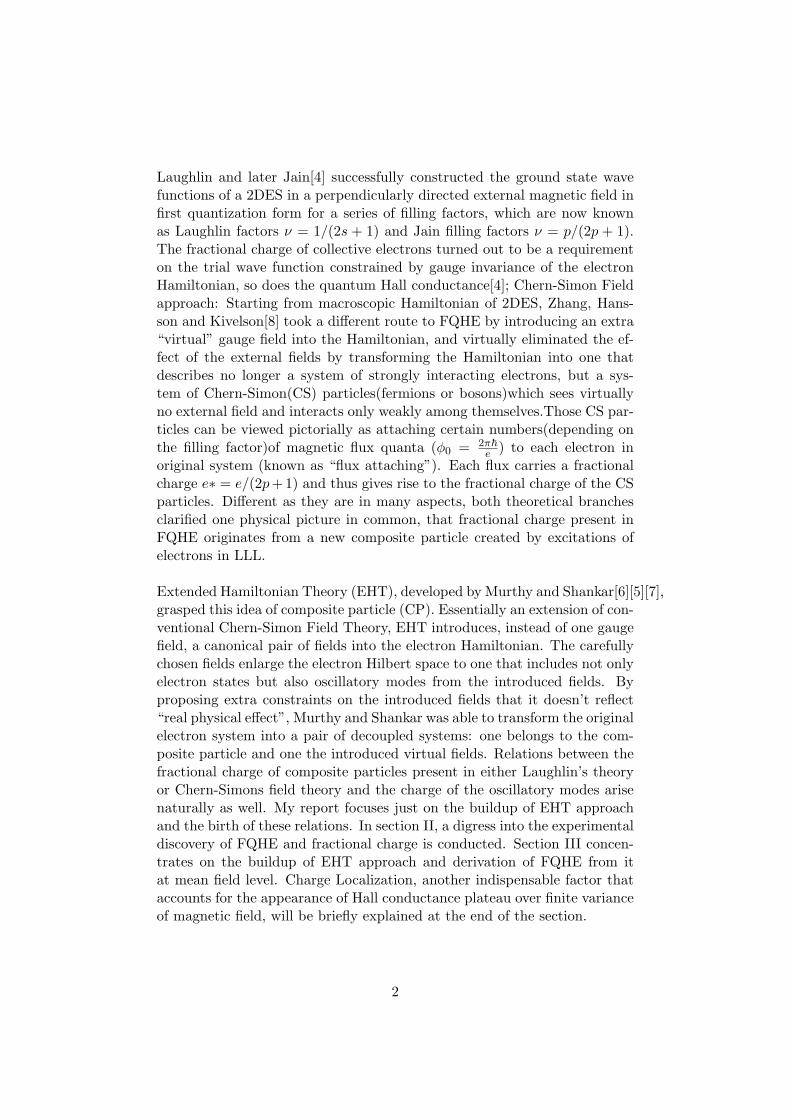
FQHE was first experimentally observed by Stormer et.al [1] in 1981.Stormer and his coworkers formulated a 2DES at the interface of twosemiconductors:GaAs and AlGaAs. Conducting electrons congregateat GaAs side of the interface and form a thin layer with µm thickness,a result of the matching of lattice structure and constants betweentwo materials and a slightly different surface electron energies (GaAshas energy level about 300meV lower than AlGaAs). The sample isprepared by modulation doping with an elaborate low electron densityand high electron mobility [1] and then exposed to Hall measurementof the resistivity tensor of the specimen. A typical result is shown in(Figure 1).

Figure 1: Experimental Observation of 1/3 FQHE: ρxy Hall resistivity, ρxx Magnetore-sistivity. The sample is modulated doped GaAs/AlGaAs[1]

Regular quantum Hall conductance plateaus appear at integral fillingfactors (ν = 1, 2, 3, · · · ), as predicted by Integral Quantum Hall Ef-fect(IQHE), which was well awared of at that time in 2DES in magnetic

3

field. A remarkable deviation from IQHE occurs at B = 15T , whereHall resistivity data forms another plateau, rather than a straight linepredicted by IQHE. Stormer et.al identified this new plateau withfractional filling factor ν = 1/3. Hall resistivity was measured threetimes high as that of IQHE at ν = 1, indicating the appearance of afractional charge q = φ0/(6π~/e2) = e/3 .

• Observation of e/3 fractional charge and FQHE at other fill-ing factors

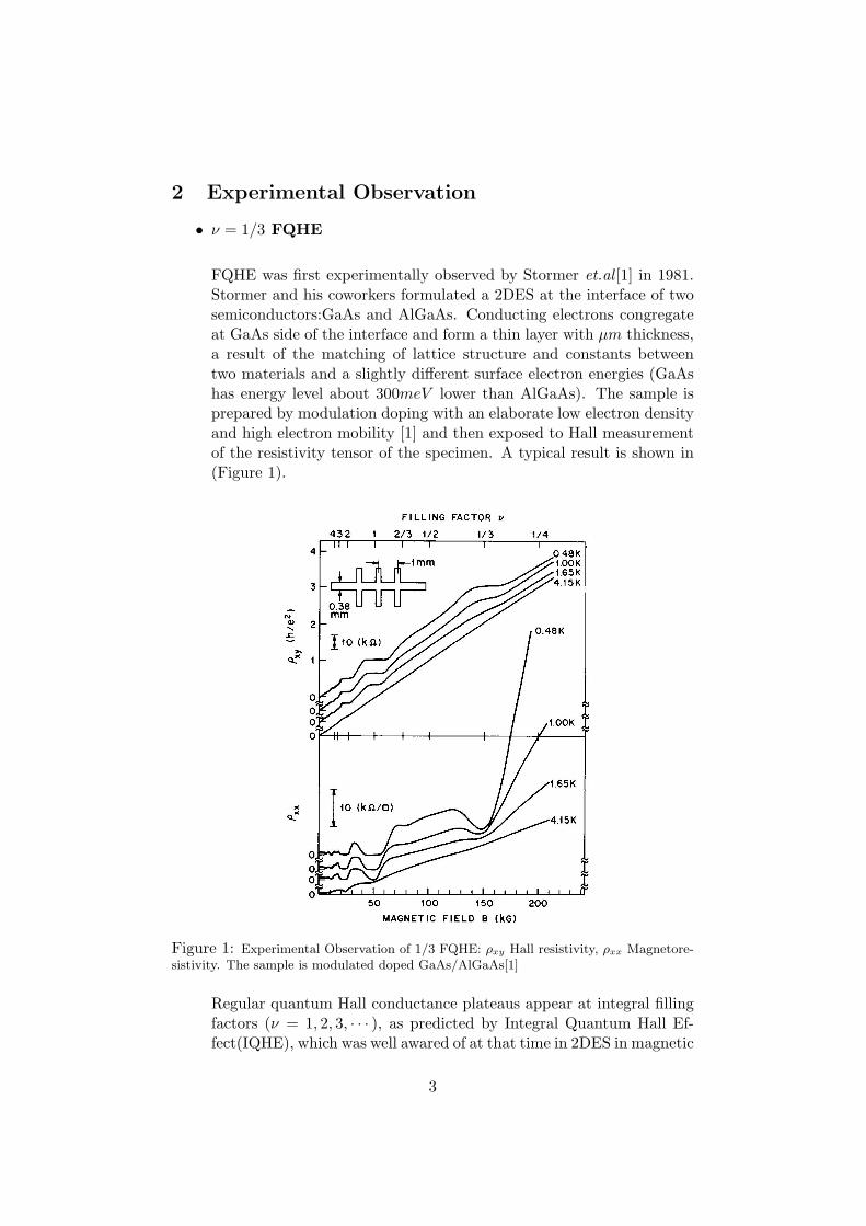
Enormous experiments following Stormer on Hall measurement of 2DESsample disclosed FQHE at other non-integral filling factors. Figure 2shows a typical sample of FQHE at various rational fraction fillingfactors[4].

Figure 2: Typical IQHE and FQHE at various filling factors, quoted from [3]

The prediction of appearance of fractional charge by Stormer in exper-iment and later on by Laughlin in his trial wave function for ν = 1/3FQHE was also convinced by following experiments of various meth-ods. Shot-noise measurements by Saminadayar et al. are one of themost widely cited. Saminadayar and his collaborators successfullymeasured the shot noise associated with tunnelling in the fractionalquantum Hall regime of a 2DES sample with filling factor ν = 1/3 [2],the experimental proof is illustrated in Figure 3.

Despite the difference in the filling factor of various FQHE, the gen-

4

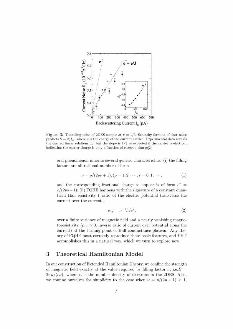
Figure 3: Tunneling noise of 2DES sample at ν = 1/3; Schottky formula of shot noisepredicts S = 2qIB , where q is the charge of the current carrier. Experimental data revealsthe desired linear relationship, but the slope is 1/3 as expected if the carrier is electron,indicating the carrier charge is only a fraction of electron charge[2]

eral phenomenon inherits several generic characteristics: (i) the fillingfactors are all rational number of form

ν = p/(2ps + 1), (p = 1, 2, · · · , s = 0, 1, · · · , (1)

and the corresponding fractional charge to appear is of form e∗ =e/(2ps+1); (ii) FQHE happens with the signature of a constant quan-tized Hall resistivity ( ratio of the electric potential transverse thecurrent over the current )

ρxy = ν−1h/e2, (2)

over a finite variance of magnetic field and a nearly vanishing magne-toresistivity (ρxx ' 0, inverse ratio of current over potential along thecurrent) at the turning point of Hall conductance plateau. Any the-ory of FQHE must correctly reproduce these basic features, and EHTaccomplishes this in a natural way, which we turn to explore now.

3 Theoretical Hamiltonian Model

In our construction of Extended Hamiltonian Theory, we confine the strengthof magnetic field exactly at the value required by filling factor ν, i.e.B =2πn/(eν), where n is the number density of electrons in the 2DES. Also,we confine ourselves for simplicity to the case when ν = p/(2p + 1) < 1,

5

i.e. all the electrons are filled up in the lowest Landau level(LLL) of thesystem and assumption that their spins are all uniformly polarized is henceimplied. We would also take a bold step to ignore Coulombic interactionsbetween electrons in the derivation. Over-simplified as it may seem, it willbe clear soon that EHT, even without introduction of interactions, has al-ready incorporated basic features of FQHE. Introduction of interactions willrefine our detailed results such as Chern-Simon wave function ψCS , but thederivation would no longer be intuitive and concise. A brief discussion of theeffect of interactions will be included at the end for completeness. Naturalunits (~ = c = 1)are applied except stated otherwise. A “cyclotron length”l0 = (eB)−1/2 is also defined in natural units, which will show up extensivelyin our derivation.

We start by writing down the Chern-Simon Hamiltonian(density) with-out interaction in second quantized form.

HCS = ψ†CS

| − i∇+ eA∗ + a|22m

ψCS (3)

where ψCS is the Chern-Simon wave function describing the composite par-ticle of electron attached with magnetic flux quanta. a is the Chern-Simongauge field that satisfies the constraint

∇× a2πl

= ψ†CSψCS = ψ†eψe = ρ

(One could well start with electron Hamiltonian and get (3) by Chern-Simonapproach, we bypass this derivation here for concision, standard referencecan be found in [6] and [8])The effect of the gauge field is to cancel the magnetic field on the average,so that for example at filling factors ν = 1/(2p + 1), Chern-Simon particlesees an effective zero-field A∗ ' 0Using the constraints on a, we transform (3) symbolically as

HCS = ψ†CS

| − i∇+ eA∗ + (∇×)−12πlρ|22m

ψCS (4)

EHT enlarges the electron Hilbert Space in the following fashion: in mo-mentum space, for each electron momentum q, EHT associate a canonicalpair of vector fields

P(q) = iqP (q), a(q) = −iz × qa(q)

and canonical commutator between the two fields,

[a(q), P (q′)] = (2π)2δ(q + q′) (5)

6

where the Dirac function is evaluated in two dimensions. Hamiltonian (4)is totally equivalent to

HCS = ψ†CS

| − i∇+ eA∗ + a + (∇×)−12πlρ|22m

ψCS (6)

provided that we restrain

a(q)|physical〉 = 0

, or[a,H] = 0

This enables us to find simultaneous eigenvalues of H and a, and that cor-responds to a = 0 solves the original problem. To set up further equivalencebetween this EHT model and original Chern-Simon model, EHT introducesa projection operator that connects the wavefunctions of these two models:

℘ =∫

dxda|x a〉〈x a|δ(a)δ(0)

(7)

The physical meaning of (7) is clear if one consider its action on a wave func-tion of the expanded Hilbert Space Ψ(x, a) (x labels the position quantumnumber of the original particle while a labels the non-physical field degreesof freedom)

Ψ℘(x, a) = ℘Ψ(x, a) =δ(a)δ(0)

Ψ(x, a) =δ(a)δ(0)

Ψ(x, 0) =δ(a)δ(0)

ΨCS(x) (8)

EHT then introduces a unitary transformation to get rid of the “inverse ofcurl” term shown in (6),

U = exp[∫

d2qiP (−q)2πl

qρ(q)] (9)

under which the Hamiltonian transforms into

H =1

2mψ†CP (−i∇+ eA∗ + a + 2πlP)2ψCP (10)

ψCS(x) = ψCP exp[∫

d2qiP (−q)2πl

qe−iqx] (11)

0 = (a− 2πlρ

q)|physical〉 (12)

Eq.(12) is just the constraint 0 = a(q)|physical〉 written in terms of trans-formed a field.

7

Expand Eq.(10)(drop the subscript CP henceforth), we get

H =1

2m|(−i∇+ eA∗)ψ|2 +

n

2m(a2 + 4π2l2P 2)

+(a + 2πlP ) · 12m

ψ†(−i︷︸︸︷∇ +eA∗)ψ

+δ(ψ†ψ)

2m(a + 2πlP)2

= H0 + H1 + H2 (13)

where ρ = ψ†ψ = 〈ψ†ψ〉 + δ(ψ†ψ) = n + δ(ψ†ψ), n stands for the averagedensity of the composite particles(which is just the average electron density),and δ(ψ†ψ) its fluctuation. Also, we define

A︷︸︸︷∇ B = A∇B − (∇A)B

Now we are finally prepared to get to the “final representation” applied inEHT. the second term in the first line of (13), or H0, resembles the ordinaryHamiltonian of quantum oscillators, with natural frequency ω0 = 2πln

m , andtherefore can be written in second quantized form by introducing ladderoperators, and the ψ operator can be replaced by creation and annihila-tion operators of composite particles in momentum space. We’ll set fill-ing factor explicitly as ν = p/(2p + 1) such that ω0 = 2p

2p+1eBm = 2p

2p+1ωc,B∗ = B/(2p + 1)(by attaching 2p + 1 flux quanta to each electron). Andwe ignore contribution from last term in (13) since we’re working at meanfield level, no fluctuation is considered to the leading order. Putting piecestogether, (13) can be reformulated as

H =∑

j

Π2j

2m+

∫d2qD†(q)D(q)ω0+

√2π

m

∫d2q(c†(q)D(q)+D†(q)c(q)) ≡ T+Hosc+H1

(14)where

Π = P + eA∗

D(q) =1√(8π)

[a(q) + 4πiP (q)]

c(q) = q−∑

j

Πj+e−iqxj

Π± = Πx ± iΠy

[D(q), D†(q′)] = (2π)2δ(q − q′)[Π−,Π+] = −2eB∗ = −2eB/(2p + 1)

[c(q), c†(q′)] = 2eB∗n(2π)2δ(q − q′), [c(q), c(q′)] = [c†(q), c†(q′)] = 0

8

Now H1 still appears as a coupling between the composite particle field andthe introduced fields.To lift this coupling, [6] conducts a further unitarytransformation,

U(λ0) = eiSλ0 = exp[√

2π

4πnλ0

∫d2q(c†(q)D(q)−D†(q)c(q))] (15)

with λ to be cleverly chosen as solution to tan(λ0/√

2p) = 1√2p

= µ and thefinal representation of the EHT Hamiltonian reads as

HFR =∑

j

Πj−Πj+

2m+

∑

j

eB∗

2m− 1

2mn

∑

i,j

∫d2qΠj−e−iq(xi−xj)Πj++

∫d2qD†(q)D(q)

eB

m

(16)Eq.(16) concludes the Hamiltonian for EHT approach, and the problem ofelectron systems in FQHE has been equivalently mapped to a systems ofcomposite particles (in present case, composite fermions since odd numberof flux quanta are attached to each electron to form the composite particle[3])and a decoupled field of oscillators. The wave function of this Hamiltonian,when projected to the subspace where the oscillator quantum number isfreezed at ground state(analogy to a = 0 in (8)), accounts correctly for thewave function of the physical composite fermions, and therefore the wavefunction of electron system in FQHE, at least at a mean field level. (Onecan actually build up Laughlin wave function solely from (13), which turnsout to be more direct than working with (16)[6]). Note, however, the de-coupling transformation (15) yields a third term in composite particle partof EHT Hamiltonian in (16), this can be shown to give rise to the desiredrenormalization of electron mass to the mass of the composite particle[6].Now let’s examine how the fractional charge and quantized Hall conductanceare embedded in (16).Electron Charge Density: Using techniques analogous to the Heisenbergequation of motion for operators and take S present in Eq.(15) as the “ef-fective Hamiltonian operator”, one gets the equation connecting the chargedensity before and after transformation as

d ρ(q, λ)λ

=q√8π

(D(q, λ) + D†(q, λ)) (17)

where ρ(q, λ) = e−iSλρ(q)eiSλ and one sees immediately that ρ(q, 0) is thecharge density before transformation to the final representation, and ρ(q, λ0)is the charge density desired in the final representation. Eq.(17) can beintegrated as

ρ(q, 0) = ρ(q, λ0)+q√8π

(sinµλ0

µ(D(q)+D†(−q))−

√2π

4πnµ2(1−cosµλ0)(c(q)+c†(q)))

(18)

9

Similar treatment with operator a(q) brings about another relation as

qa(q, 0)4π

=q√8π

(cosµλ0(D(q)+D†(−q))−√

2π

4πnµsinµλ0(c(q)+c†(q))) (19)

(all the operators in Eq.(18)(19) are before unitary transformation)Why bother writing down those lengthy expressions? The reason lies in thatdue to constraint condition ρ(q, 0) = qa(q,0)

4π as stated earlier, any combina-tion

γρ(q, 0) + (1− γ)qa(q, 0)

4π(20)

is physically equivalent and acceptable as a charge density operator of EHTHamiltonian (16). EHT excludes this degeneracy of choice of γ by requiringthat the charge density should satisfy magnetic translation algebra, proposedby Girvin, Jach and GMP[6], whose details are beyond our interest. Whatthis algebra brings about is a unique choice of γ in (20) as γ = 1/(2p + 1)for the filling factor we’re considering. And the charge density under thischoice is, by working out explicitly expression for c(q),

ρ(q, 0) =q√8π

cosµλ0(D(q)+D†(−q))+1

2p + 1

∑

j

e−iqxj−il20∑

j

(q×Πj)e−iqxj

(21)The first term counts for the virtual charge of the oscillatory field, the thirdterm is a dipolar term indicating possible nonzero dipole of the compositefermions in our system, and the second term, in great analogy to electroncharge density ρe(q) = e

∑j e−iqxj for N charged particles sitting at {xj}|Nj=1,

is our desired CHARGE of the composite fermion, and the fractional chargee∗ = e/(2p + 1) is readily observed.Quantized Hall Conductance: To find the Hall conductance ,we applysimilar technique as in (18)(19) here to find the current operator

J(q, 0) =∑

j

(Πj

me−iqxj +

n

m

√8π(q)D(q)) (22)

in final representation. Carry out the equation of motion for J(q, λ), wehave

J(q, 0) =qeBcosµλ0√

2πm2D(q) (23)

Remarkably, the current is carried entirely by the oscillator! The cancel-lation of particle contribution to current leads eventually to a surprisinglysimple derivation of the Hall conductance.We recall that physical state of the EHT Hamiltonian has no contributionfrom the oscillatory field, i.e. it must be in the ground state of the oscillatorpart of the Hamiltonian. Calculation of Hall conductance σxy) in this caseamounts to calculate the ground state average of D(q) when the oscillator is

10

coupled with an external electric field. the coupling term is no surprise of theform − ∫

d2xeρ(x)Φ(x) = − ∫d2qeρ(−q)Φ(q). We apply Eq.(21) for ρ(−q)

and concentrate only on the oscillatory part of ρ, since no contribution ofthe current is from composite fermions, and get

Hosc =∫

d2qeB/mD†(q)D(q)− e

∫d2qρ(−q)Φ(q)

=∫

d2qeB/mD†(q)D(q)− e

∫d2qΦ(q)

q√8π

cosµλ0(D(q) + D†(−q))

=∫

d2qeB

m[D†(q)− qmcosµλ0√

8πBΦ(−q)] · [D(q)− qmcosµλ0√

8πBΦ(q)]

+∫

d2qeBq2cos2µλ0

8πmΦ(−q)Φ(q) (24)

last term in (24) is just a constant and can be ignored, the first term indicatesno more than a shift in the zero of D(q), and therefore,

〈D(q)〉 =qmcosµλ0√

8πBΦ(q)

the electric current in momentum space of the physical state is thus

〈(−e)J(q)〉 = (−e)qeBcosµλ0√

2πm2〈D(q)〉 = −e2ν

hqΦ(q) = −e2ν

hE(q) (25)

Eq.(25) yields no doubt the correct Hall conductance σxy = e2νh (in consis-

tency with Eq.(2)).Charge localization and Hall conductance plateau: Point feature ofFQHE in 2DES, namely fractional charge and quantization of Hall conduc-tance, has been explored to details using EHT. Yet the existence of Hallconductance plateau involves more factors than what we have discussedhere. It is believed[3][4] that existence of such a plateau is attributed solelyto the complexity of the interaction of the electron system, in the presenceof IMPURITIES in 2DES. The effect of impurities, which is inevitable inreal 2DES sample, is to couple to the electron system a fluctuating or ran-dom potential. The influence of the potential can be formulated briefly asfollows: due to random potential or potential fluctuation in the 2DES, thesharply seperated Landau levels of the electron system, or of the compositeparticle system are broadened into Landau bands. Yet the new energy levelsgenerated by the broadening correspond mostly to localized particle states(the so-called Anderson Localization effect[3]) and does not contribute tolong distance conducting property of the 2DES. Hence the excess of com-posite particles(fermions or bosons) created by slightly increasing magneticfield from its filling factor value are correlated and localized with the impu-rities in the sample in FQHE (In IQHE, it is the excess of electrons that are

11

localized.), making no contribution to the conductivity of the system, andthe Hall conductance remains constant at its quantized value, until the vari-ation in the magnetic field is big enough for system to overcome energy gapsbetween FQHE at different filling factors and transit to FQHE at anotherpreferred quantized state.

4 Summary and Conclusion

The construction of Extended Hamiltonian Theory, as an extension of con-ventional Chern-Simon field theory approach is reviewed at a non-interacting,mean field level. Features of FQHE such as fractional charge of the compos-ite particle and quantized Hall conductance is verified using EHT Hamil-tonian. Electron system in EHT is essentially expanded into two decou-pled systems, one describing the physical composite particles which emergesthrough flux attachment process of electrons, the other non-physical oscil-lator Hamiltonian which has no explicit affect on real physical states, reg-ulating the particle part of EHT Hamiltonian only implicitly. real FQHEinvolves not only correlations within electrons but also between electronsand impurities in the sample, which accounts heavily for the localization oflow-excitation levels of electrons or composite particles(fermions or bosons)and the plateau of Hall conductance over a finite variance of magnetic field.Coulombic interactions of electrons, which is bypassed in the article, actuallyaccounts for the renormalization of electron mass at low excited compositeparticle Landau level (beyond LLL), and the compressibility property of the2DES system[6][7][8]. In general, FQHE emerges in electron systems withbroken translational symmetry (low dimension and impurities) as a resultof collective behavior of electrons. The fractional charge phenomenon andthe success of gauge field theory approach in understanding FQHE impliessurprisingly that “fractional quantum number and powerful gauge forces be-tween these particles can arise spontaneously as emergent phenomena”, asquoted Laughlin[4].

References

[1] D.Tsui, H.L.Stormer, A.C.Gossard, Phys.Rev.Lett. 48,1559(1982)

[2] L.Saminadayar, D.C. Glattli, Phys.Rev.Lett. 79,2526(1997)

[3] H.L.Stormer, Rev.Mod.Phys. Vol.71,No.4(1999)

[4] R.B.Laughlin, Rev.Mod.Phys. Vol.71,No.4(1999)

[5] G.Murthy, R.Shankar, Rev.Mod.Phys. Vol.75,No.4(2003)

[6] G.Murthy, R.Shankar, cond-mat/9802244

12

[7] R.Shankar, G.Murthy, Phys.Rev.Lett.79, 4437(1997)

[8] Low Dimensional Quantum Field Theories for Condensed MatterPhysicists, edited by S.Lundqvist, et.al.

13