fpo - sage publications inc | home...tistics identified here: • descriptive statistics: applying...

1 Introduction to Statistics

Learning ObjectivesAfter reading this chapter, you should be able to:

1. Distinguish between descriptive and inferential statistics.

2. Explain how samples and populations, as well as a sample statistic and population parameter, differ.

3. Describe three research methods commonly used in behavioral science.

4. State the four scales of measurement and provide an example for each.

5. Distinguish between variables that are qualitative or quantitative.

6. Distinguish between variables that are discrete or continuous.

7. Enter data into SPSS by placing each group in separate columns and each group in a single column (coding is required).

iStock / thumb

FPO

Draft P

roof -

Do not

copy

, pos

t, or d

istrib

ute

Copyright ©2018 by SAGE Publications, Inc. This work may not be reproduced or distributed in any form or by any means without express written permission of the publisher.

Chapter 1: Introduction to Statistics 3

Chapter Outline1.1 The Use of Statistics in Science1.2 Descriptive and Inferential Statistics1.3 Research Methods and Statistics1.4 Scales of Measurement

1.5 Types of Variables for Which Data Are Measured

1.6 Research in Focus: Evaluating Data and Scales of Measurement

1.7 SPSS in Focus: Entering and Defining Variables

1.1 The Use of sTaTisTics in scienceWhy should you study statistics? The topic can be intimidating, and rarely does anyone tell you, “Oh, that’s an easy course . . . take statistics!” Statistics is a branch of mathematics used to summarize, analyze, and interpret what we observe—to make sense or meaning of our observations. Really, statistics is used to make sense of the observations we make. For example, we can make sense of how good a soccer player is by observing how many goals he or she scores each season, and we can understand cli-mates by looking at average temperature. We can also understand change by looking at the same statistics over time—such as the number of goals scored by a soccer player in each game, and the average temperature over many decades.

Statistics is commonly applied to evaluate scientific observations. Scientific observations are all around you. Whether you are making deci-sions about what to eat (based on health statistics) or how much to spend (based on the behavior of global markets), you are making decisions based on the statistical evaluation of scientific observations. Scientists who study human behavior gather information about all sorts of behavior of interest to them, such as information on addiction, happiness, worker productivity, resiliency, faith, child development, love, and more. The information that scientists gather is evaluated in two ways; each way reveals the two types of statistics taught in this book:

• Scientists organize and summarize information such that the infor-mation is meaningful to those who read about the observations scientists made in a study. This type of evaluation of information is called descriptive statistics.

• Scientists use information to answer a question (e.g., is diet related to obesity?) or make an actionable decision (e.g., should we imple-ment a public policy change that can reduce obesity rates?). This type of evaluation of information is called inferential statistics.

This book describes how to apply and interpret both types of sta-tistics in science and in practice to make you a more informed inter-preter of the statistical information you encounter inside and outside of the classroom. For a review of statistical notation (e.g., summation notation) and a basic math review, please see Appendix A. The chapter organization of this book is such that descriptive statistics are described

Statistics is a branch of mathematics used to summarize, analyze, and interpret a group of numbers or observations.

Master the content.edge.sagepub.com/priviterastats3e

Draft P

roof -

Do not

copy

, pos

t, or d

istrib

ute


4 Part I: Introduction and Descriptive Statistics

in Chapters 2–4 and applications for probability are further introduced in Chapters 5–7, to transition to a discussion of inferential statistics in the remainder of the book in Chapters 8–18.

The reason it is important to study statistics can be described by the words of Mark Twain: There are lies, damned lies, and statistics. He meant that statistics could be deceiving, and so can interpreting them. Statistics are all around you—from your college grade point average (GPA) to a Newsweek poll predicting which political candidate is likely to win an election. In each case, statistics are used to inform you. The challenge as you move into your careers is to be able to identify statistics and to interpret what they mean. Statistics are part of your everyday life, and they are subject to interpretation. The interpreter, of course, is you.

In many ways, statistics allow a story to be told. For example, your GPA may reflect the story of how well you are doing in school; the Newsweek poll may tell the story of which candidate is likely to win an election. In storytelling, there are many ways to tell a story. Similarly, in statistics, there are many ways to evaluate the information gathered in a study. For this reason, you will want to be a critical consumer of the information you come across, even information that is scientific. In this book, you will learn the fundamentals of statistical evaluation, which can help you to critically evaluate any information presented to you.

In this chapter, we begin by introducing the two general types of sta-tistics identified here:

• Descriptive statistics: applying statistics to organize and summa-rize information

• Inferential statistics: applying statistics to interpret the meaning of information

1.2 DescripTive anD inferenTial sTaTisTicsThe research process typically begins with a question or statement that can only be answered or addressed by making an observation. The obser-vations researchers make are typically recorded as data (i.e., numeric values). To illustrate, Figure 1.1 describes the general structure for making scientific observations, using an example to illustrate. As a basic example adapted from larger-scale studies looking at obesity and healthy food choice (Capaldi & Privitera, 2008; Privitera, 2016a), suppose a researcher asks if adding sugar to a sour-tasting fruit juice (a grapefruit juice) can increase intake of this healthy juice. To test this question, the researcher first identifies a group of participants who dislike plain grape-fruit juice and sets up a research study to create two groups: Group No Sugar (this group drinks the grapefruit juice without any added sugar), and Group Sugar (this group drinks the grapefruit juice with sugar added). In this study, the researcher measures intake (i.e., how much juice is consumed). Suppose she decides to measure amount consumed in milli-liters (note: 30 milliliters equals about 1 ounce). The data in this example are the volume of drink consumed in milliliters. If adding sugar increases

FYITwo types of statistics are descriptive statistics and inferential statistics.

Data (plural) are a set of scores, measurements, or observations that are typically numeric. A datum (singular) is a single measurement or observation, usually referred to as a score or raw score.

Draft P

roof -

Do not

copy

, pos

t, or d

istrib

ute



intake of grapefruit juice, then we expect that participants will consume more of the grapefruit juice when sugar is added (i.e., Group Sugar will consume more milliliters of the juice than Group No Sugar).

In this section, we will introduce how descriptive and inferential statis-tics allow researchers to assess the data they measure in a research study, using the example given here and in Figure 1.1.

Descriptive StatisticsOne way in which researchers can use statistics in research is to use proce-dures developed to help organize, summarize, and make sense of measure-ments or data. These procedures, called descriptive statistics, are typically used to quantify the behaviors researchers measure. Thus, we measure or record data (e.g., milliliters consumed), then use descriptive statistics to summarize or make sense of those data, which describe the phenome-non of interest (e.g., intake of a healthy fruit juice). In our example, intake could be described simply as amount consumed, which certainly describes intake, but not numerically—or in a way that allows us to record data on intake. Instead, we stated that intake is milliliters consumed of the juice. Here, we define intake as a value that can be measured numerically; hence,

FIGURE 1.1 General Structure for Making Scientific Observations

• [1] Ask a question

• [2] Set-up a research study

Does addingsugar to a grapefruit

juice increaseintake of the juice?

Select participantsand create groups:two groups drink

grapefruit juice; onewith and one without

sugar added.

Measure amountconsumed of thegrapefruit juice in

milliliters.

Compare amountconsumed ineach group.

• [4] Evaluate findings

• [3] Measure behavior

The general structure for making scientific observations, using an example for testing if adding sugar increases intake of a grapefruit juice.

Descriptive statistics are procedures used to summarize, organize, and make sense of a set of scores called data. Descriptive statistics are typically presented graphically, in tabular form (in tables), or as summary statistics (single values).

Draft P

roof -

Do not

copy

, pos

t, or d

istrib

ute



intake can now be measured. If we observe hundreds of participants, then the data in a spreadsheet will be overwhelming. Presenting a spreadsheet with the intake for each individual participant is not very clear. For this rea-son, researchers use descriptive statistics to summarize sets of individual measurements so they can be clearly presented and interpreted.

Data are generally presented in summary. Typically, this means that data are presented graphically, in tabular form (in tables), or as summary statistics (e.g., an average). For example, instead of listing each individ-ual measure of intake, we could summarize the average (mean), middle (median), or most common (mode) amount consumed in milliliters among all participants, which can be more meaningful.

Tables and graphs serve a similar purpose to summarize large and small sets of data. One particular advantage of tables and graphs is that they can clarify findings in a research study. For example, to evaluate the findings for our study, we expect that participants will consume more grapefruit juice in milliliters if sugar is added to the juice. Figure 1.2 dis-plays these expected findings. Notice how summarizing the average intake in each group in a figure can clarify research findings.

FIGURE 1.2 Summary of Expected Findings

0

50

100

150

200

250

300

350

Sugar No Sugar

Ave

rag

e I

nta

ke (

in m

illilite

rs)

Groups

A graphical summary of the expected findings if adding sugar increases intake of a grapefruit juice.

Inferential StatisticsMost research studies include only a select group of participants, and not all participants who are members of a particular group of interest. In other words, most scientists have limited access to the phenomena they study, especially behavioral phenomena. Hence, researchers select a por-tion of all members of a group (the sample) mostly because they do not have access to all members of a group (the population). Imagine, for exam-ple, trying to identify every person who has experienced exam anxiety.

Draft P

roof -

Do not

copy

, pos

t, or d

istrib

ute



The same is true for most behaviors—the population of all people who exhibit those behaviors is likely too large. Because it is often not possible to identify all individuals in a population, researchers require statistical procedures, called inferential statistics, to infer that observations made with a sample are also likely to be observed in the larger population from which the sample was selected.

To illustrate, we can continue with the grapefruit juice study. If we are interested in all those who have a general dislike for sour-tasting grape-fruit juice, then this group would constitute the population of interest. Specifically, we want to test if adding sugar increases intake of a grape-fruit juice in this population; this characteristic (intake of a grapefruit juice) in the population is called a population parameter. Intake, then, is the characteristic we will measure, but not in the population. In practice, researchers will not have access to an entire population. They simply do not have the time, money, or other resources to even consider studying all those who have a general dislike for sour-tasting grapefruit juice.

An alternative to selecting all members of a population is to select a portion or sample of individuals in the population. Selecting a sample is more practical, and most scientific research is based upon findings in sam-ples, not populations. In our example, we can select any portion of those who have a general dislike for sour-tasting grapefruit juice from the larger population; the portion of those we select will constitute our sample. A characteristic that describes a sample, such as intake, is called a sample statistic and is the value that is measured in a study. A sample statistic is measured to estimate the population parameter. In this way, a sample is selected from a population to learn more about the characteristics in a population of interest.

Inferential statistics are procedures used that allow researchers to infer or generalize observations made with samples to the larger population from which they were selected.

A population is the set of all individuals, items, or data of interest. This is the group about which scientists will generalize.

A characteristic (usually numeric) that describes a population is called a population parameter.

A sample is a set of individuals, items, or data selected from a population of interest.

A characteristic (usually numeric) that describes a sample is referred to as a sample statistic.

FYIInferential statistics are used to help the

researcher infer how well statistics in a sample reflect parameters

in a population.

MAKING SENSE POPULATIONS AND SAMPLES

A population is identified as any group of interest, whether that group is all students worldwide or all students in a professor’s class. Think of any group you are interested in. Maybe you want to understand why college students join fraternities and sororities. So students who join fraternities and sororities is the group you are interested in. Hence, to you, this group is a population of interest. You identified a population of interest just as researchers identify populations they are interested in.

Remember that researchers select samples only because they do not have access to all individuals in a population. Imagine having to identify every person who has fallen in love, experienced anxiety, been attracted to someone else, suffered with depression, or taken a college exam. It is ridiculous to consider that

we can identify all individuals in such populations. So researchers use data gathered from samples (a portion of individuals from the population) to make inferences concerning a population.

To make sense of this, suppose you want to get an idea of how people in general feel about a new pair of shoes you just bought. To find out, you put your new shoes on and ask 20 people at random throughout the day whether or not they like the shoes. Now, do you really care about the opinion of only those 20 people you asked? Not really—you actually care more about the opinion of people in general. In other words, you only asked the 20 people (your sample) to get an idea of the opinions of people in general (the population of interest). Sampling from populations follows a similar logic.

Draft P

roof -

Do not

copy

, pos

t, or d

istrib

ute



Example 1.1 applies the process of sampling to distinguish between a sample and a population.

Example 1.1

On the basis of the following example, we will identify the population, sample, population parameter, and sample statistic: Suppose you read an article in the local college newspaper citing that the average college student plays 2 hours of video games per week. To test whether this is true for your school, you randomly approach 20 fellow students and ask them how long (in hours) they play video games per week. You find that the average student, among those you asked, plays video games for 1 hour per week. Distinguish the population from the sample.

In this example, all college students at your school constitute the population of interest, and the 20 students you approached is the sample that was selected from this population of interest. Because it is purported that the average college student plays 2 hours of video games per week, this is the population parameter (2 hours). The average number of hours playing video games in the sample is the sample statistic (1 hour).

Answers: 1. Descriptive statistics; 2. b; 3. c; 4. True.

1.3 research MeThoDs anD sTaTisTicsThis book will describe many ways of measuring and interpreting data. Yet, simply collecting data does not make you a scientist. To engage in science, you must follow specific procedures for collecting data. Think of this as playing a game. Without the rules and procedures for play-ing, the game itself would be lost. The same is true in science; without the rules and procedures for collecting data, the ability to draw scien-tific conclusions would be lost. Ultimately, statistics are often used in the

LEARNING CHECK 1

1. _____________ are procedures used to summarize, organize, and make sense of a set of scores called data.

2. __________ describe(s) characteristics in a population, whereas _____________ describe(s) characteristics in a sample.

(a) Statistics; parameters

(b) Parameters; statistics

(c) Descriptive; inferential

(d) Inferential; descriptive

3. A psychologist wants to study a small population of 40 students in a local private school. If the researcher

was interested in selecting the entire population of students for this study, then how many students must the psychologist include?

(a) None, because it is not possible to study an entire population in this case.

(b) At least half, because this would constitute the majority of the population.

(c) All 40 students, because all students constitute the population.

4. True or false: Inferential statistics are used to help the researcher infer the unknown parameters in a given population.

Draft P

roof -

Do not

copy

, pos

t, or d

istrib

ute



context of science. In the behavioral sciences, science is specifically applied using the research method. To use the research method, we make observations using systematic techniques of scientific inquiry. In this section, we introduce three research methods that are commonly applied in the behavioral sciences.

To illustrate the basic premise of engaging in sci-ence, suppose you come across the following prob-lem first noted by the famous psychologist Edward Thorndike in 1898:

Dogs get lost hundreds of times and no one ever notices it or sends an account of it to a scientific magazine, but let one find his way from Brook-lyn to Yonkers and the fact immediately becomes a circulating anecdote. Thousands of cats on thousands of occasions sit helplessly yowling, and no one takes thought of it or writes to his friend, the professor; but let one cat claw at the knob of a door supposedly as a signal to be let out, and straightway this cat becomes the rep-resentative of the cat-mind in all books. . . . In short, the anecdotes give really . . . supernormal psychology of animals. (pp. 4–5)

Here the problem was to determine the animal mind. Thorndike posed the question of whether animals were truly smart, based on the many observations he made. This is where the scientific process typically begins: with a question. To answer questions in a scientific manner, researchers need more than just statistics; they need a set of strict procedures for making the obser-vations and measurements. In this section, we introduce three research methods commonly used in behavioral research: experimental, quasi- experimental, and correlational methods. Each method involves examining the relationship between variables, and these methods are introduced here because we will apply them throughout the book.

Experimental MethodOften, the aims of a researcher are to demonstrate a causal relationship (i.e., that one variable causes changes in another variable). Any study that can demonstrate cause is called an experiment. To demonstrate cause, though, an experiment must follow strict procedures to ensure that all other possible causes are eliminated or highly unlikely. Hence, researchers must control the conditions under which observations are made in order to isolate cause-and-effect relationships between variables. Figure 1.3 shows the general structure of an experiment using an example to illustrate the structure that is described.

Figure 1.3 illustrates a basic example adapted from larger-scale studies looking at metacognition and memory recall (Diemand-Yauman,

© Ca

n Sto

ck Ph

oto I

nc. /

iofot

o

Science is the study of phenomena, such as behavior, through strict observation, evaluation, interpretation, and theoretical explanation.

The research method, or scientific method, is a set of systematic techniques used to acquire, modify, and integrate knowledge concerning observable and measurable phenomena.

An experiment is the use of methods and procedures to make observations in which a researcher fully controls the conditions and experiences of participants by applying three required elements of control (manipulation, randomization, and comparison/control) to isolate cause-and-effect relationships between variables.

Draft P

roof -

Do not

copy

, pos

t, or d

istrib

ute



Oppenheimer, & Vaughan, 2011; Price, McElroy, & Martin, 2016). Here we evaluate if writing key terms in bold (just like we do in this book in each chapter) improves recall of those words. A sample of students at a similar reading level was selected from a population of college undergraduates. In one group, students read a short passage with 10 bolded key terms; in the other group, students read the same short passage but with the 10 key terms in regular font. After reading each passage, students were asked to write down as many key terms as they could recall. The number of correct key terms listed was recorded for each group.

For this study to be called an experiment, researchers must satisfy three requirements. These requirements are regarded as necessary steps to ensure enough control to allow researchers to draw cause-and-effect conclusions. These requirements are the following:

Population

Sample

Not bolded condition:students read the sameshort passage with the

10 key terms in regular font.

Manipulate one variable,called the independentvariable—randomly assignparticipants to each levelof the manipulated variable.

Example: Randomlyassign participants to twolevels of Bolding.

Record number of keyterms correctly recalled

from the passage.

Record number of keyterms correctly

recalled from the passage.

Measure a second variable,called the dependent variable—the same variable is measuredin each condition and thedifference betweengroups is compared.

Example: Record the numberof key terms correctlyrecalled from the passagein each condition.

Bolded condition:students read a short

passage with 10 key termsin bold font.

FIGURE 1.3 The Basic Structure of an Experiment

The basic structure of an experiment that meets each basic requirement for demonstrating cause and effect using an example of a study in which a sample of students at a similar reading level was selected at random from a population of college undergraduates to test if bolding key terms in a short passage improves recall. To qualify as an experiment, (1) the researcher created each level of the bolding/not bolding independent variable (manipulation), (2) students were randomly assigned to read a passage with or without bolded key terms (randomization), and (3) a control group was present where the manipulation of bolding the key terms was absent (comparison/control).

Draft P

roof -

Do not

copy

, pos

t, or d

istrib

ute



1. Manipulation (of variables that operate in an experiment)

2. Randomization (of assigning participants to conditions)

3. Comparison/control (a control group)

To meet the requirement of randomization, researchers must use random assignment (Requirement 2) to assign participants to groups. To do this, a researcher must be able to manipulate the levels of an independent variable (IV) (Requirement 1) to create the groups. Referring back to the key term bolding example shown in Figure 1.3, the independent variable was bolding. The researcher first manipulated the levels of this variable (bolded, regular font), meaning that she created the conditions. She then assigned students at a similar reading level at random to experience one of the lev-els of distraction. As an example of random assignment, the researcher could select participant names at random from names written on pieces of paper in a bowl—with every other participant name selected assigned to the experimental (bold font) group, and all others to the control group (regular font group).

Random assignment and manipulation ensure that characteristics of participants in each group (such as their age, intelligence level, or study habits) vary entirely by chance. Because participant characteristics in both groups now occur at random, we can assume that these character-istics are about the same in both groups. This makes it more likely that any differences observed between groups were caused by the manipula-tion (bolded vs. regular font key terms in a passage) and not participant characteristics.

Notice also that there are two groups in the experiment shown in Figure 1.3. The number of correct key terms listed after reading the pas-sage was recorded and can be compared in each group. By comparing the number of correct key terms listed in each group, we can determine whether bolding the key terms caused better recall of the key terms com-pared to those who read the same passage without bolded key terms. This satisfies the requirement of comparison (Requirement 3), which requires that at least two groups be observed in an experiment so that scores in one group can be compared to those in at least one other group.

In this example, recall of key terms was recorded in each group. The measured or recorded variable in an experiment is called the dependent variable (DV). Dependent variables can often be measured in many ways, and therefore often require an operational definition. An operational defi-nition is a description for how a dependent variable was measured. For example, here we operationally defined recall as the number of key terms correctly listed after reading a passage (students could recall 0 to all 10 key terms). Thus, we measured the dependent variable as a number. To sum-marize the experiment in Figure 1.3, bolding key terms (IV) was presumed to cause an effect or difference in recall (DV) between groups. This is an experiment in which the researcher satisfied the requirements of manipula-tion, randomization, and comparison/control, thereby allowing her to draw cause-and-effect conclusions, assuming the study was properly conducted.

Random assignment is a random procedure used to ensure that participants in a study have an equal chance of being assigned to a particular group or condition.

An independent variable (IV) is the variable that is manipulated in an experiment. This variable remains unchanged (or “independent”) between conditions being observed in an experiment. It is the “presumed cause.” The specific conditions of an IV are referred to as the levels of the independent variable.

The dependent variable (DV) is the variable that is measured in each group of a study, and it is believed to change in the presence of the independent variable. It is the “presumed effect.”

An operational definition is a description of some observable event in terms of the specific process or manner by which it was observed or measured.

FYIAn experiment is a study in which

researchers satisfy three requirements to ensure enough control to allow them to draw cause-and-effect conclusions.

These are manipulation, randomization, and comparison/control.

Draft P

roof -

Do not

copy

, pos

t, or d

istrib

ute



MAKING SENSE EXPERIMENTAL AND CONTROL GROUPS

While a comparison group is sometimes necessary, it is preferred that, when possible, a control group be used. By definition, a control group must be treated exactly the same as an experimental group, except that the members of this group do not actually receive the treatment believed to cause changes in the dependent variable. As an example, suppose we hypothesize that rats will dislike flavors that are associated with becoming ill (see Garcia, Kimeldorf, & Koelling, 1955; Privitera, 2008). To test this hypothesis, the rats in an experimental group receive a vanilla-flavored drink followed by an injection of lithium chloride to make them ill. The rats in a control group must be treated the same, minus the manipulation of administering lithium chloride to make them ill. In a control group, then, rats receive the same vanilla-flavored drink also followed by an injection, but in this group the substance injected is inert, such as a saline solution (called a placebo). The next day, we record how much vanilla-flavored solution rats consume during a brief test (in milliliters).

Note that simply omitting the lithium chloride is not sufficient. The control group in our example still receives an injection; otherwise, both being injected and the substance that is injected will differ between groups. Other important factors for experiments like these include some control of the diets rats consume before and during the study, and to ensure that many other environmental factors are the same for all rats, such as their day-night sleep cycles and housing arrangements. These added levels of control ensure that both groups are truly identical, except that one group is made ill and a second group is not. In this way, researchers can isolate all factors in an experiment, such that only the manipulation that is believed to cause an effect is different between groups. This same level of consideration must be made in human experiments to ensure that groups are treated the same, except for the factor that is believed to cause changes in the dependent variable.

Quasi-Experimental MethodA research study that is structured similar to an experiment but meets one or both of the following two conditions is called a quasi-experiment:

1. The study does not include a manipulated independent variable.

2. The study lacks a comparison/control group.

In a typical quasi-experiment, the variables being studied cannot be manipulated, which makes random assignment impossible. This occurs when variables are preexisting or inherent to the participants themselves. A preexisting variable, or one to which participants cannot be randomly assigned, is called a quasi-independent variable. Figure 1.4 shows an example of a quasi-experiment that measured differences in multitasking ability by sex. Because participants cannot be randomly assigned to the levels of sex (male, female), sex is a quasi-independent variable, and this study is therefore regarded as a quasi-experiment.

A study is also regarded as a quasi-experiment when only one group is observed. With only one group, there is no comparison or control group, which means that differences between two levels of an independent vari-able cannot be compared. In this way, failing to satisfy any of the require-ments for an experiment makes the study a quasi-experiment when the study is otherwise structured similar to an experiment.

A quasi-independent variable is a preexisting variable that is often a characteristic inherent to an individual, which differentiates the groups or conditions being compared in a research study. Because the levels of the variable are preexisting, it is not possible to randomly assign participants to groups.

FYIA quasi-experiment is a study that (1) includes a quasi-independent variable and/or (2) lacks a comparison/control group.

Draft P

roof -

Do not

copy

, pos

t, or d

istrib

ute



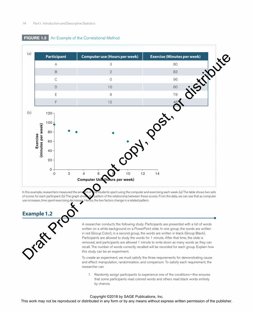
Correlational MethodAnother method for examining the relationship between variables is to mea-sure pairs of scores for each individual. This method can determine whether a relationship exists between variables, but it lacks the appropriate controls needed to demonstrate cause and effect. To illustrate, suppose you test for a relationship between times spent using a computer and exercising per week. The data for such a study appear in tabular form and are plotted as a graph in Figure 1.5. Using the correlational method, we can examine the extent to which two variables change in a related fashion. In the example shown in Figure 1.5, as computer use increases, time spent exercising decreases. This pattern suggests that computer use and time spent exercising are related.

Notice that no variable is manipulated to create different conditions or groups to which participants can be randomly assigned. Instead, two variables are measured for each participant, and the extent to which those variables are related is measured. Thus, the correlational method does not at all control the conditions under which observations are made and is therefore not able to demonstrate cause-and-effect conclusions. This book describes many statistical procedures used to analyze data using the correlational method (Chapters 15–17) and the experimental and quasi-experimental methods (Chapters 8–14 and 17–18).

Example 1.2 applies a research example to identify how a research design can be constructed.

Sex is not randomly assigned. Men are assigned to the male condition; women to the female condition.

A sample of men and women is selected from a population.

Male condition:Men are asked to completeas many tasks as possible

in 5 minutes.

Female condition:Women are asked to complete

as many tasks as possiblein 5 minutes.

Dependent measure:The number of tasks

completed is recorded.

Dependent measure:The number of tasks

completed is recorded.

FIGURE 1.4 The Basic Structure of a Quasi-Experiment

In this example, researchers measured differences in multitasking behavior by sex. The grouping variable (sex) is preexisting. That is, participants were already male or female prior to the study. For this reason, researchers cannot manipulate the variable or randomly assign participants to each level of sex, so this study is regarded as a quasi-experiment.

FYIThe correlational method can

determine whether a relationship exists between variables, but it lacks the controls needed to demonstrate

cause and effect.

Draft P

roof -

Do not

copy

, pos

t, or d

istrib

ute



Example 1.2

A researcher conducts the following study: Participants are presented with a list of words written on a white background on a PowerPoint slide. In one group, the words are written in red (Group Color); in a second group, the words are written in black (Group Black). Participants are allowed to study the words for 1 minute. After that time, the slide is removed, and participants are allowed 1 minute to write down as many words as they can recall. The number of words correctly recalled will be recorded for each group. Explain how this study can be an experiment.

To create an experiment, we must satisfy the three requirements for demonstrating cause and effect: manipulation, randomization, and comparison. To satisfy each requirement, the researcher can

1. Randomly assign participants to experience one of the conditions—this ensures that some participants read colored words and others read black words entirely by chance;

Participant Computer use (Hours per week) Exercise (Minutes per week)

A 3 80

B 2 83

C 0 96

D 10 60

E 8 78

F 12 46

(a)

Exe

rcis

e(m

inu

tes

per

week)

Computer Use (hours per week)

120

100

80

60

40

20

00 2 4 6 8 10 12 14

(b)

FIGURE 1.5 An Example of the Correlational Method

In this example, researchers measured the amount of time students spent using the computer and exercising each week. (a) The table shows two sets of scores for each participant. (b) The graph shows the pattern of the relationship between these scores. From the data, we can see that as computer use increases, time spent exercising decreases. Hence, the two factors change in a related pattern.

Draft P

roof -

Do not

copy

, pos

t, or d

istrib

ute



2. Create the two conditions that are identical, except for the color manipulation—the researcher can write the same 20 words on two PowerPoint slides, on one slide in red and on the second slide in black; and

3. Include a comparison group—in this case, the number of colored (red) words correctly recalled will be compared to the number of black words correctly recalled, so this study has a comparison group.

Remember that each requirement is necessary to demonstrate that the levels of an independent variable are causing changes in the value of a dependent variable. If any one of these requirements is not satisfied, then the study is not an experiment.

Answers: 1. Science; 2. a. Experiment. b. Quasi-experiment. c. Correlational method; 3. True.

1.4 scales of MeasUreMenTMany statistical tests introduced in this book will require that variables in a study be measured on a certain scale of measurement. In the early 1940s, Harvard psychologist S. S. Stevens coined the terms nominal, ordinal, interval, and ratio to classify scales of measurement (Stevens, 1946). Scales of measurement are rules that describe the properties of numbers. These rules imply that the extent to which a number is informative depends on how it was used or measured. In this section, we discuss the extent to which data are informative on each scale of measurement. In all, scales of measurement are characterized by three properties: order, difference, and ratio. Each property can be described by answering the following questions:

1. Order: Does a larger number indicate a greater value than a smaller number?

2. Difference: Does subtracting two numbers represent some mean-ingful value?

3. Ratio: Does dividing (or taking the ratio of) two numbers represent some meaningful value?

©iS

tock

phot

o.com

/skv

oor

Scales of measurement identify how the properties of numbers can change with different uses. Four scales of measurement are nominal, ordinal, interval, and ratio.

To Come

LEARNING CHECK 2

1. ____________ is the study of phenomena through strict observation, evaluation, interpretation, and theoretical explanation.

2. State whether each of the following describes an experiment, a quasi-experiment, or a correlational method.

(a) A researcher tests whether the dosage level of some drug (low, high) causes significant differences in health.

(b) A researcher tests whether citizens of differing political affiliations (Republican, Democrat) will show differences in attitudes toward morality.

(c) A researcher measures the relationship between annual income and life satisfaction.

3. True or false: An experiment is the only method that can demonstrate cause-and-effect relationships between variables.

Draft P

roof -

Do not

copy

, pos

t, or d

istrib

ute



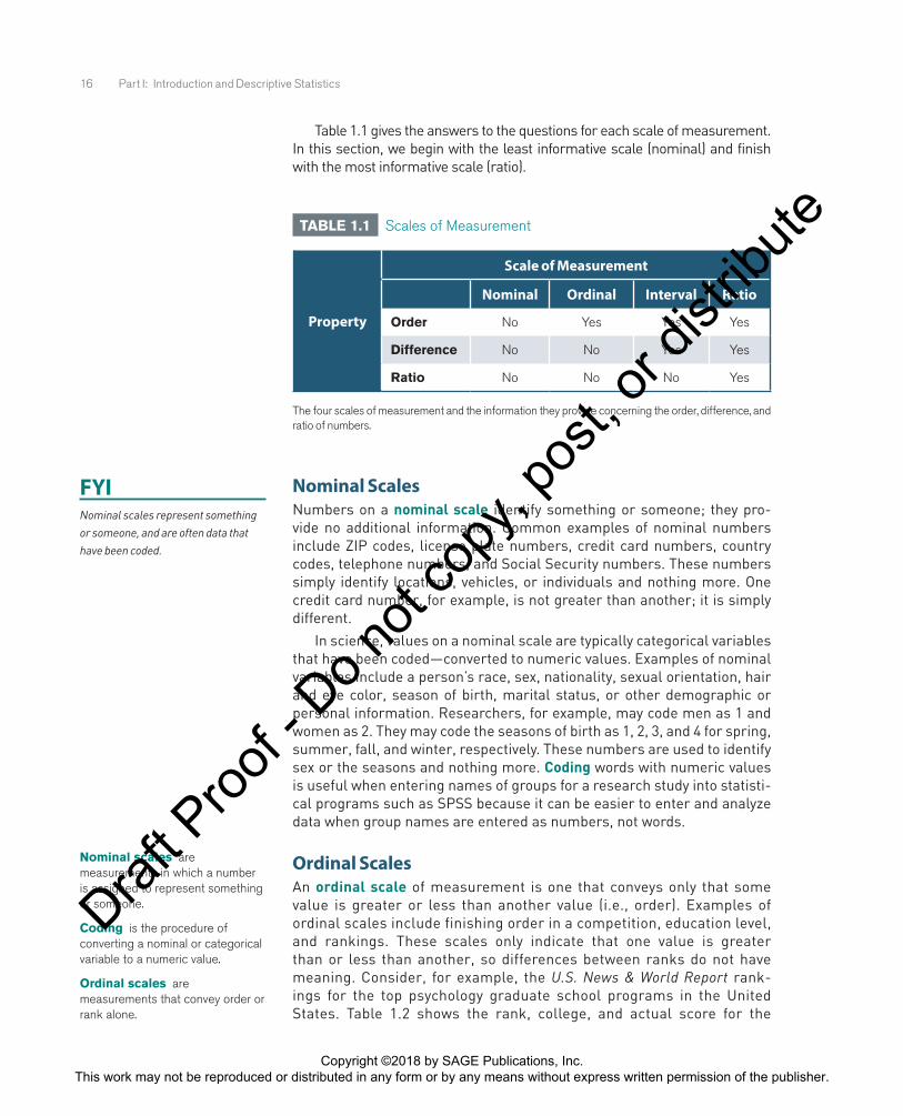
Table 1.1 gives the answers to the questions for each scale of measurement. In this section, we begin with the least informative scale (nominal) and finish with the most informative scale (ratio).

TABLE 1.1 Scales of Measurement

Property

Scale of Measurement

Nominal Ordinal Interval Ratio

Order No Yes Yes Yes

Difference No No Yes Yes

Ratio No No No Yes

The four scales of measurement and the information they provide concerning the order, difference, and ratio of numbers.

Nominal ScalesNumbers on a nominal scale identify something or someone; they pro-vide no additional information. Common examples of nominal numbers include ZIP codes, license plate numbers, credit card numbers, country codes, telephone numbers, and Social Security numbers. These numbers simply identify locations, vehicles, or individuals and nothing more. One credit card number, for example, is not greater than another; it is simply different.

In science, values on a nominal scale are typically categorical variables that have been coded—converted to numeric values. Examples of nominal variables include a person’s race, sex, nationality, sexual orientation, hair and eye color, season of birth, marital status, or other demographic or personal information. Researchers, for example, may code men as 1 and women as 2. They may code the seasons of birth as 1, 2, 3, and 4 for spring, summer, fall, and winter, respectively. These numbers are used to identify sex or the seasons and nothing more. Coding words with numeric values is useful when entering names of groups for a research study into statisti-cal programs such as SPSS because it can be easier to enter and analyze data when group names are entered as numbers, not words.

Ordinal ScalesAn ordinal scale of measurement is one that conveys only that some value is greater or less than another value (i.e., order). Examples of ordinal scales include finishing order in a competition, education level, and rankings. These scales only indicate that one value is greater than or less than another, so differences between ranks do not have meaning. Consider, for example, the U.S. News & World Report rank-ings for the top psychology graduate school programs in the United States. Table 1.2 shows the rank, college, and actual score for the

FYINominal scales represent something or someone, and are often data that have been coded.

Nominal scales are measurements in which a number is assigned to represent something or someone.

Coding is the procedure of converting a nominal or categorical variable to a numeric value.

Ordinal scales are measurements that convey order or rank alone.

Draft P

roof -

Do not

copy

, pos

t, or d

istrib

ute



top 25 programs, including ties, in 2013. Based on ranks alone, can we say that the difference between the psychology graduate programs ranked 1 and 7 is the same as the difference between those ranked 14 and 21? No. In both cases, 7 ranks separate the schools. However, if you look at the actual scores for determining rank, you find that the difference between ranks 1 and 7 is 0.3 points, whereas the difference between ranks 14 and 21 is 0.1 points. So the difference in points is not the same. Ranks alone do not convey this difference. They simply indicate that one rank is greater than or less than another rank.

TABLE 1.2 Ordinal Scale Data for College Rankings

Rank College Name Actual Score

1 2 2 4 4 4 7 7 9 9 91212141414141414142121212121

Stanford UniversityUniversity of California, BerkeleyUniversity of California, Los AngelesHarvard UniversityUniversity of Michigan, Ann ArborYale UniversityUniversity of Illinois at Urbana-ChampaignPrinceton UniversityUniversity of Minnesota, Twin CitiesUniversity of Wisconsin–MadisonMassachusetts Institute of TechnologyUniversity of PennsylvaniaUniversity of North Carolina at Chapel HillUniversity of Texas at AustinUniversity of WashingtonWashington University in St. LouisUniversity of California, San DiegoColumbia UniversityCornell UniversityNorthwestern UniversityThe Ohio State UniversityCarnegie Mellon UniversityDuke UniversityUniversity of California, DavisUniversity of Chicago

4.84.74.74.64.64.64.54.54.44.44.44.34.34.24.24.24.24.24.24.24.14.14.14.14.1

A list of the U.S. News & World Report rankings for the top 25 psychology graduate school programs in the United States in 2013, including ties (left column), and the actual points used to determine their rank (right column).

Source: http://grad-schools.usnews.rankingsandreviews.com/best-graduate-schools.

Interval ScalesAn interval scale of measurement can be understood readily by two defin-ing principles: equidistant scales and no true zero. A common example for this in behavioral science is the rating scale. Rating scales are taught here

FYIOrdinal scales convey order alone.

Interval scales are measurements that have no true zero and are distributed in equal units.

Draft P

roof -

Do not

copy

, pos

t, or d

istrib

ute


http://grad-schools.usnews.rankingsandreviews.com/best-graduate-schools


as an interval scale because most researchers report these as interval data in published research. This type of scale is a numeric response scale used to indicate a participant’s level of agreement with or opinion of some statement. An example of a rating scale is given in Figure 1.6. Here we will look at each defining principle.

An equidistant scale is a scale with intervals or values distributed in equal units. Many behavioral scientists assume that scores on a rating scale are distributed in equal units. For example, if you are asked to rate your satisfaction with a spouse or job on a 7-point scale from 1 (completely unsatisfied) to 7 (completely satisfied), then you are using an interval scale, as shown in Figure 1.6. By assuming that the distance between each point (1 to 7) is the same or equal, it is appropriate to compute differences between scores on this scale. So a statement such as “The difference in job satisfaction among men and women was 2 points” is appropriate with interval scale measurements.

However, an interval scale does not have a true zero. A common exam-ple of a scale without a true zero is temperature. A temperature equal to zero for most measures of temperature does not mean that there is no temperature; it is just an arbitrary zero point. Values on a rating scale also have no true zero. In the example shown in Figure 1.6, 1 was used to indicate no satisfaction, not 0. Each value (including 0) is arbitrary. That is, we could use any number to represent none of something. Measurements of latitude and longitude also fit this criterion. The implication is that with-out a true zero, there is no outright value to indicate the absence of the phenomenon you are observing (so a zero proportion is not meaningful). For this reason, stating a ratio such as “Satisfaction ratings were three times greater among men compared to women” is not appropriate with interval scale measurements.

Ratio ScalesRatio scales are similar to interval scales in that scores are distributed in equal units. Yet, unlike interval scales, a distribution of scores on a ratio scale has a true zero. This is an ideal scale in behavioral research because any mathematical operation can be performed on the values that are mea-sured. Common examples of ratio scales include counts and measures of length, height, weight, and time. For scores on a ratio scale, order is infor-mative. For example, a person who is 30 years old is older than another who is 20. Differences are also informative. For example, the difference

FYIAn interval scale is equidistant but has no true zero.

An equidistant scale is a set of numbers distributed in equal units.

A true zero is when the value 0 truly indicates nothing on a scale of measurement. Interval scales do not have a true zero.

Ratio scales are measurements that have a true zero and are distributed in equal units.

Satisfaction Ratings

1 2 3 4 5 6 7

Completely Unsatisfied Completely Satisfied

FIGURE 1.6 An Example of a 7-Point Rating Scale for Satisfaction Used for Scientific InvestigationDraft P

roof -

Do not

copy

, pos

t, or d

istrib

ute



between 70 and 60 seconds is the same as the difference between 30 and 20 seconds (the difference is 10 seconds). Ratios are also informative on this scale because a true zero is defined—it truly means nothing. Hence, it is meaningful to state that 60 pounds is twice as heavy as 30 pounds.

In science, researchers often go out of their way to measure variables on a ratio scale. For example, if they measure hunger, they may choose to measure the amount of time between meals or the amount of food con-sumed (in ounces). If they measure memory, they may choose to mea-sure the amount of time it takes to memorize some list or the number of errors made. If they measure depression, they may choose to measure the dosage (in milligrams) that produces the most beneficial treatment or the number of symptoms reported. In each case, the behaviors are measured using values on a ratio scale, thereby allowing researchers to draw conclu-sions in terms of order, differences, and ratios—there are no restrictions for variables measured on a ratio scale.

FYIA ratio scale is equidistant and has a

true zero, and it is the most informative scale of measurement.

Answers: 1. Scales of measurement; 2. Ordinal; 3. d; 4. Movie ratings (from 1 to 4 stars).

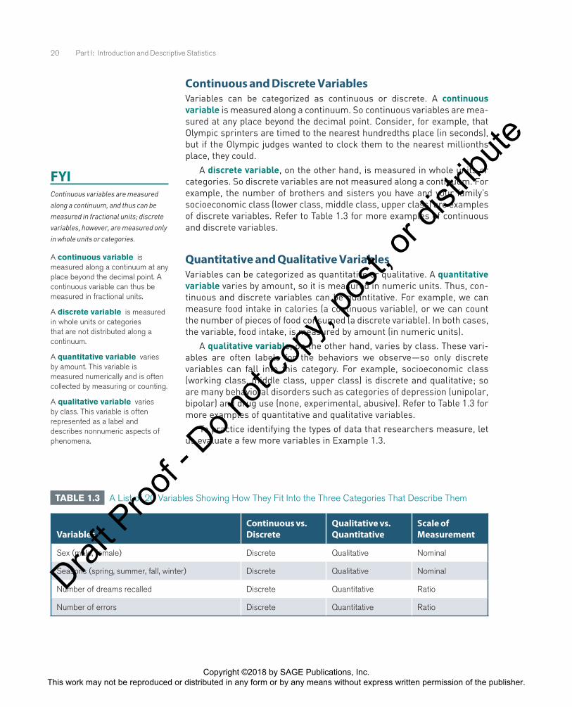
1.5 Types of variables for Which DaTa are MeasUreDScales of measurement reflect the informativeness of data. With nomi-nal scales, researchers can conclude little; with ratio scales, researchers can conclude just about anything in terms of order, difference, and ratios. Researchers also distinguish between the types of data they measure. The variables for which researchers measure data fall into two broad categories: (1) continuous or discrete and (2) quantitative or qualitative. Each category is discussed in this section. Many examples to help you delineate these categories are given in Table 1.3.

LEARNING CHECK 3

1. ____________ are rules for how the properties of numbers can change with different uses.

2. In 2010, Fortune magazine ranked Apple as the most admired company in the world. This ranking is on a(n) ____________ scale of measurement.

3. What are two characteristics of rating scales that allow researchers to use these values on an interval scale of measurement?

(a) Values on an interval scale have a true zero but are not equidistant.

(b) Values on an interval scale have differences and a true zero.

(c) Values on an interval scale are equidistant and have a true zero.

(d) Values on an interval scale are assumed to be equidistant but do not have a true zero.

4. A researcher measures four variables: age (in days), speed (in seconds), height (in inches), and movie ratings (from 1 to 4 stars). Which of these variables is not an example of a variable measured on a ratio scale?

Draft P

roof -

Do not

copy

, pos

t, or d

istrib

ute



Continuous and Discrete VariablesVariables can be categorized as continuous or discrete. A continuous variable is measured along a continuum. So continuous variables are mea-sured at any place beyond the decimal point. Consider, for example, that Olympic sprinters are timed to the nearest hundredths place (in seconds), but if the Olympic judges wanted to clock them to the nearest millionths place, they could.

A discrete variable, on the other hand, is measured in whole units or categories. So discrete variables are not measured along a continuum. For example, the number of brothers and sisters you have and your family’s socioeconomic class (lower class, middle class, upper class) are examples of discrete variables. Refer to Table 1.3 for more examples of continuous and discrete variables.

Quantitative and Qualitative VariablesVariables can be categorized as quantitative or qualitative. A quantitative variable varies by amount, so it is measured in numeric units. Thus, con-tinuous and discrete variables can be quantitative. For example, we can measure food intake in calories (a continuous variable), or we can count the number of pieces of food consumed (a discrete variable). In both cases, the variable, food intake, is measured by amount (in numeric units).

A qualitative variable, on the other hand, varies by class. These vari-ables are often labels for the behaviors we observe—so only discrete variables can fall into this category. For example, socioeconomic class (working class, middle class, upper class) is discrete and qualitative; so are many behavioral disorders such as categories of depression (unipolar, bipolar) and drug use (none, experimental, abusive). Refer to Table 1.3 for more examples of quantitative and qualitative variables.

To practice identifying the types of data that researchers measure, let us evaluate a few more variables in Example 1.3.

FYIContinuous variables are measured along a continuum, and thus can be measured in fractional units; discrete variables, however, are measured only in whole units or categories.

A continuous variable is measured along a continuum at any place beyond the decimal point. A continuous variable can thus be measured in fractional units.

A discrete variable is measured in whole units or categories that are not distributed along a continuum.

A quantitative variable varies by amount. This variable is measured numerically and is often collected by measuring or counting.

A qualitative variable varies by class. This variable is often represented as a label and describes nonnumeric aspects of phenomena.

TABLE 1.3 A List of 20 Variables Showing How They Fit Into the Three Categories That Describe Them

VariablesContinuous vs. Discrete

Qualitative vs. Quantitative


Sex (male, female) Discrete Qualitative Nominal

Seasons (spring, summer, fall, winter) Discrete Qualitative Nominal

Number of dreams recalled Discrete Quantitative Ratio

Number of errors Discrete Quantitative Ratio

Draft P

roof -

Do not

copy

, pos

t, or d

istrib

ute



VariablesContinuous vs. Discrete

Qualitative vs. Quantitative


Duration of drug abuse (in years) Continuous Quantitative Ratio

Ranking of favorite foods Discrete Quantitative Ordinal

Ratings of satisfaction (1 to 7) Discrete Quantitative Interval

Body type (slim, average, heavy) Discrete Qualitative Nominal

Score (from 0% to 100%) on an exam Continuous Quantitative Ratio

Number of students in your class Discrete Quantitative Ratio

Temperature (degrees Fahrenheit) Continuous Quantitative Interval

Time (in seconds) to memorize a list Continuous Quantitative Ratio

The size of a reward (in grams) Continuous Quantitative Ratio

Position standing in line Discrete Quantitative Ordinal

Political affiliation (Republican, Democrat) Discrete Qualitative Nominal

Type of distraction (auditory, visual) Discrete Qualitative Nominal

A letter grade (A, B, C, D, F) Discrete Qualitative Ordinal

Weight (in pounds) of an infant Continuous Quantitative Ratio

A college student’s SAT score Discrete Quantitative Interval

Number of lever presses per minute Discrete Quantitative Ratio

Example 1.3

For each of the following examples, (1) name the variable being measured, (2) state whether the variable is continuous or discrete, and (3) state whether the variable is quantitative or qualitative.

a. A researcher records the month of birth among patients with schizophrenia. The month of birth (the variable) is discrete and qualitative.

b. A professor records the number of students absent during a final exam. The number of absent students (the variable) is discrete and quantitative.

c. A researcher asks children to choose which type of cereal they prefer (one with a toy inside or one without). He records the choice of cereal for each child. The choice of cereal (the variable) is discrete and qualitative.

d. A therapist measures the time (in hours) that clients continue a recommended program of counseling. The time in hours (the variable) is continuous and quantitative.

Draft P

roof -

Do not

copy

, pos

t, or d

istrib

ute



LEARNING CHECK 4

1. True or false: A ratio scale variable can be continuous or discrete.

2. State whether each of the following is continuous or discrete.

(a) Delay (in seconds) it takes drivers to make a left-hand turn when a light turns green

(b) Number of questions that participants ask during a research study

(c) Type of drug use (none, infrequent, moderate, or frequent)

(d) Season of birth (spring, summer, fall, or winter)

3. State whether the variables listed in Question 2 are quantitative or qualitative.

4. True or false: Qualitative variables can be continuous or discrete.

5. A researcher is interested in the effects of stuttering on social behavior with children. He records the number of peers a child speaks to during a typical school day. In this example, would the data be qualitative or quantitative?

Answers: 1. True; 2. a. Continuous. b. Discrete. c. Discrete. d. Discrete; 3. a. Quantitative. b. Quantitative. c. Qualitative. d. Qualitative; 4. False. Qualitative variables can only be discrete; 5. Quantitative.

1.6 RESEARCH IN FOCUS: EVALUATING DATA AND SCALES OF MEASUREMENT

While qualitative variables are often measured in behavioral research, this book will focus largely on quantitative variables. The reason is twofold: (1) Quantitative measures are more common in behavioral research, and (2) most statistical tests taught in this book are adapted for quantitative measures. Indeed, many researchers who measure qualitative variables will also measure those that are quantitative in the same study.

For example, Jones, Blackey, Fitzgibbon, and Chew (2010) explored the costs and benefits of social networking among college students. The researchers used a qualitative method to interview each student in their sample. In the interview, students could respond openly to questions asked during the interview. These researchers then summarized responses into categories related to learning, studying, and social life. For example, the following student response was categorized as an example of independent learning experience for employability: “I think it [social software] can be beneficial . . . in the real working environment” (Jones et al., 2010, p. 780).

The limitation for this analysis is that categories are on a nominal scale (the least informative scale). So many researchers who record qualitative data also use some quantitative measures. For example, researchers in this study also asked students to rate their usage of a variety of social software technologies, such as PowerPoint and personal websites, on a scale from 1 (never)

© iS

tock

phot

o.com

/Peo

pleIm

ages

Draft P

roof -

Do not

copy

, pos

t, or d

istrib

ute



to 4 (always). A fifth choice (not applicable) was also included on this rating scale. These ratings are on an interval scale, which allowed the researchers to also discuss differences related to how much students used social software technologies.

Inevitably, the conclusions we can draw with qualitative data are rather limited because these data are typically on a nominal scale. On the other hand, most statistics introduced in this book require that variables be measured on the more informative scales. For this reason, this book mainly describes statistical procedures for quantitative variables measured on an ordinal, interval, or ratio scale.

1.7 SPSS in Focus: Entering and Defining Variables

Throughout this book, we present instructions for using the statistical software program SPSS by showing you how this software can make all the work you do by hand as simple as point and click. Before you read this SPSS section, please take the time to read the section titled “How to Use SPSS With This Book” at the beginning of this book. That section provides an overview of the different views and features in SPSS. This software is an innovative statistical computer program that can compute any statistic taught in this book.

In this chapter, we discussed how variables are defined, coded, and measured. Let us see how SPSS makes this simple. Keep in mind that the Variable View display is used to define the variables you measure, and the Data View display is used to enter the scores you measured. When enter-ing data, make sure that all values or scores are entered in each cell of the Data View spreadsheet. The biggest challenge is making sure you enter the data correctly. Entering even a single value incorrectly can alter the data analyses that SPSS computes. For this reason, always double-check the data to make sure the correct values have been entered.

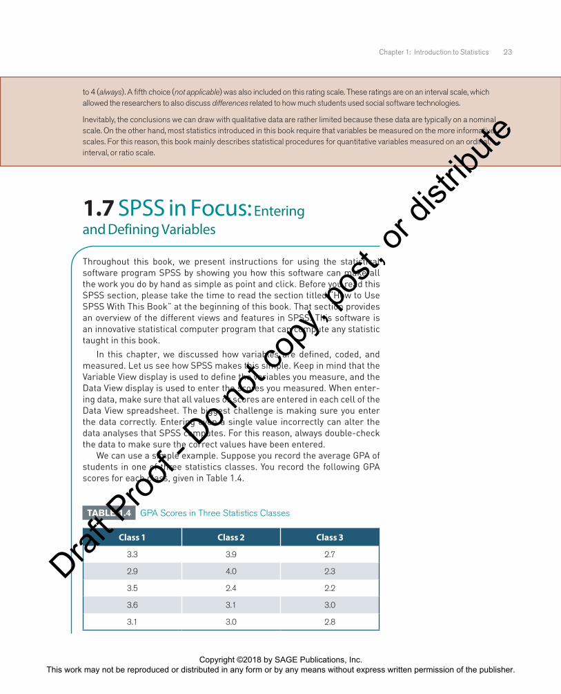
We can use a simple example. Suppose you record the average GPA of students in one of three statistics classes. You record the following GPA scores for each class, given in Table 1.4.

TABLE 1.4 GPA Scores in Three Statistics Classes

Class 1 Class 2 Class 3

3.3 3.9 2.7

2.9 4.0 2.3

3.5 2.4 2.2

3.6 3.1 3.0

3.1 3.0 2.8

Draft P

roof -

Do not

copy

, pos

t, or d

istrib

ute



There are two ways you can enter these data: by column or by row. To enter data by column:

1. Open the Variable View tab, shown in Figure 1.7. In the Name column, enter your variable names as class1, class2, and class3 (note that spaces are not allowed) in each row. Three rows should be active.

2. Because the data are to the tenths place, go to the Decimals column and reduce that value to 1 in each row.

3. Open the Data View tab. Notice that the first three columns are now labeled with the group names, as shown in Figure 1.8. Enter the data, given in Table 1.4, for each class in the appropriate column. The data for each group are now listed down each column.

FIGURE 1.7 SPSS Variable View for Entering Data by Column

FIGURE 1.8 Data Entry in SPSS Data View for Entering Data by Column

Draft P

roof -

Do not

copy

, pos

t, or d

istrib

ute



There is another way to enter these data in SPSS: You can enter data by row. This requires coding the data. To begin, open a new SPSS data file and follow the instructions given here:

1. Open the Variable View tab, shown in Figure 1.9 with the coding (we will code in Step 3) already completed. Enter classes in the first row in the Name column. Enter GPA in the second row in the Name column.

2. Go to the Decimals column and reduce the value to 0 for the first row. You will see why we did this in the next step. Reduce the Dec-imals column value to 1 in the second row because we will enter GPA scores for this variable.

FIGURE 1.9 SPSS Variable View for Entering Data by Row

FIGURE 1.10 SPSS Variable View for Entering Data by Row

Draft P

roof -

Do not

copy

, pos

t, or d

istrib

ute



3. Go to the Values column and click on the small gray box with three dots. In the dialog box shown in Figure 1.10, enter 1 in the Value cell and class 1 in the Label cell, and then select Add. Repeat these steps by entering 2 for class 2 and 3 for class 3; then select OK. When you go back to the Data View tab, SPSS will now recognize 1 as class 1, 2 as class 2, and so on in the row you labeled classes (you can see how this looks in Figure 1.9 with the coding completed for the classes variable).

4. Open the Data View tab. In the first column, enter 1 five times, 2 five times, and 3 five times. This tells SPSS that there are five students in each class. In the second col-umn, enter the corresponding GPA scores for each class by row. This data entry is shown in Figure 1.11. The data are now entered by row.

The data for all the variables are labeled, coded, and entered. If you do this correctly, SPSS will make summarizing, com-puting, and analyzing any statistic taught in this book fast and simple.

FIGURE 1.11 SPSS Data View for Entering Data by Row

chapTer sUMMary

LO 1–2: Distinguish between descriptive and inferential statistics; explain how samples and populations, as well as a sample statistic and population parameter, differ.• Statistics is a branch of mathemat-

ics used to summarize, analyze, and interpret a group of numbers or observations. Descriptive statistics are procedures used to summarize, organize, and make sense of a set of scores called data—typically pre-sented graphically, in tabular form (in tables), or as summary statistics

(single values). Inferential statistics are procedures that allow research-ers to infer whether observations made with samples are also likely to be observed in the population.

• A population is a set of all individuals, items, or data of interest. A charac-teristic that describes a population is called a population parameter. A sample is a set of individuals, items, or data selected from a population of interest. A characteristic that des-cribes a sample is called a sample statistic.

Draft P

roof -

Do not

copy

, pos

t, or d

istrib

ute



LO 3: Describe three research methods commonly used in behavioral science.• The experimental design uses manipu-

lation, randomization, and comparison/control to ensure enough control to allow researchers to draw cause-and-effect conclusions. The quasi- experimental design is structured similar to an experiment but lacks randomization and/or a comparison/ control group.

• The correlational method is used to measure pairs of scores for each individual and examine the relation-ship between the variables.

LO 4: State the four scales of measurement and provide an example for each.• Scales of measurement identify how

the properties of numbers can change with different uses. Scales are char-acterized by three properties: order, difference, and ratio. There are four scales of measurement: nominal, ordinal, interval, and ratio. Nominal scales are typically coded (e.g., sea-sons, months, sex), ordinal scales indicate order alone (e.g., rankings, grade level), interval scales have equi-distant scales and no true zero (e.g., rating scale values, temperature), and ratio scales are also distributed in

equal units but have a true zero (e.g., weight, height, calories).

LO 5–6: Distinguish between variables that are qualitative or quantitative; distinguish between variables that are discrete or continuous.• A continuous variable is measured

along a continuum, whereas a dis-crete variable is measured in whole units or categories. Hence, contin-uous but not discrete variables are measured at any place beyond the decimal point. A quantitative variable varies by amount, whereas a qualita-tive variable varies by class.

LO 7: Enter data into SPSS by placing each group in separate columns and each group in a single column (coding is required).• SPSS can be used to enter and define

variables. All variables are defined in the Variable View tab. The val-ues recorded for each variable are listed in the Data View tab. Data can be entered by column or by row in the Data View tab. Listing data by row requires coding the variable. Variables are coded in the Variable View tab in the Values column (for more details, see Section 1.7).

Key TerMscodingcontinuous variabledatadatumdependent variable (DV)descriptive statisticsdiscrete variableequidistant scaleexperimentindependent variable (IV)inferential statistics

interval scalelevels of the independent variablenominal scaleoperational definitionordinal scalepopulationpopulation parameterqualitative variablequantitative variablequasi-independent variablerandom assignment

ratio scaleraw scoreresearch methodsamplesample statisticscales of measurementsciencescientific methodscorestatisticstrue zero

Draft P

roof -

Do not

copy

, pos

t, or d

istrib

ute



enD-of-chapTer probleMs

Factual Problems

1. What is the difference between descriptive and inferential statistics?

2. Distinguish between data and a raw score.

3. By definition, how is a sample related to a population?

4. State three commonly used research methods in behavioral science.

5. In an experiment, researchers measure two types of variables: independent and dependent variables.

(a) Which variable is manipulated to create the groups?

(b) Which variable is measured in each group?

6. State the four scales of measurement. Which scale of measurement is the most informative?

7. Can a nominal variable be numeric? Explain.

8. What is the main distinction between variables on an interval scale and those on a ratio scale of measurement?

9. A quantitative variable varies by ________; a qualitative variable varies by ________.

10. What are the two types of variables that can be quantitative?

Concept and Application Problems

11. State whether each of the following words best describes descriptive statistics or inferential statistics.

(a) Describe

(b) Infer

(c) Summarize

12. State whether each of the following is true or false.

(a) Graphs, tables, and summary statistics all illustrate the application of inferential statistics.

(b) Inferential statistics are procedures used to make inferences about a population, given only a limited amount of data.

(c) Descriptive statistics can be used to describe populations and samples of data.

13. A researcher measured behavior among all individuals in a small population. Are inferen-tial statistics necessary to draw conclusions concerning this population? Explain.

14. Appropriately use the terms sample and pop-ulation to describe the following statement: A statistics class has 25 students enrolled, but only 23 students attended class.

15. On occasion, a sample can be larger than the population from which it was selected. Explain why this cannot be true.

16. A researcher demonstrates that eating breakfast in the morning causes increased alertness throughout the day. What research design must the researcher have used in this example? Explain.

17. A researcher measures the height and income of participants and finds that taller men tend to earn greater incomes than do shorter men. What type of research method did the researcher use in this example? Explain.

18. State whether each of the following variables is an example of an independent variable or a quasi-independent variable. Only answer quasi-independent for variables that cannot be randomized.

(a) Marital status

(b) Political affiliation

(c) Time of delay prior to recall

(d) Environment of research setting

(e) Years of education

(f) Type of feedback (negative, positive)

Draft P

roof -

Do not

copy

, pos

t, or d

istrib

ute



19. To determine whether a new sleeping pill was effective, adult insomniacs received a pill (either real or fake), and their sleeping times were subsequently measured (in minutes) during an overnight observation period.

(a) Identify the independent variable in this study.

(b) Identify the dependent variable in this study.

20. A researcher tests whether cocaine use increases impulsive behavior in a sample of cocaine-dependent and cocaine-inexperienced mice.

(a) Identify the independent variable in this study.

(b) Identify the dependent variable in this study.

21. Researchers are interested in studying whether personality is related to the month in which someone was born.

(a) What scale of measurement is the month of birth?

(b) Is it appropriate to code the data? Explain.

22. Rank the scales of measurement in order from least informative to most informative.

23. What is the main disadvantage of measuring qualitative data? In your answer, also explain

why quantitative research is most often applied in the behavioral sciences.

24. State whether each of the following describes a study measuring a qualitative or quantitative variable.

(a) A researcher distributes open-ended questions to participants asking how they feel when they are in love.

(b) A researcher records the blood pressure of participants during a task meant to induce stress.

(c) A psychologist interested in drug addic-tion injects rats with an attention-inducing drug and then measures the rate of lever pressing.

(d) A witness to a crime gives a description of the suspect to the police.

25. State whether each of the following is an example of a continuous or discrete variable.

(a) Time in seconds to memorize a list of words

(b) Number of students in a statistics class

(c) Weight in pounds of newborn infants

(d) SAT scores among college students

26. Fill in the table below to identify the character-istics of each variable.

VariableQualitative vs. Quantitative

Continuous vs. Discrete


Sex

Seasons

Time of day

Rating scale score

Movie ratings (1 to 4 stars)

Number of students in your class

Temperature (degrees Fahrenheit)

Time (in minutes) to prepare dinner

Position standing in line

Draft P

roof -

Do not

copy

, pos

t, or d

istrib

ute



Problems in Research

27. Gun ownership in the United States. Data from Gallup polls over a 40-year period show how gun ownership in the United States has changed. The results are described in the table below, with the percent of Americans who own guns given in each of 5 decades:

Year %

1972 43

1982 42

1992 48

2002 40

2012 43

Source: Reported at http://www.gallup.com/poll/1645/ Guns.aspx.

(a) Are the percentages reported here an example of descriptive statistics or inter-ferential statistics?

(b) Based on the percentages given in the table, how has gun ownership in the United States changed over the past 40 years?

28. The curiosity of a child. Jirout and Klahr (2012) were interested in understanding how to charac-terize and study curiosity in children. In their arti-cle, they note, “Although curiosity is an undeniably important aspect of children’s cognitive develop-ment, a universally accepted [way to measure] curiosity does not exist” (Jirout & Klahr, 2012, p. 125). What type of definition, according to these authors, is needed for the term curiosity?

29. Sex and mental toughness. Nicholls, Polman, Levy, and Backhouse (2009) measured mental

toughness (among other measures) in a sample of athletes ranging in age from 15 to 58 years. They reported that “males scored significantly higher than females on total mental tough-ness” (Nicholls et al., 2009, p. 74). Is it possible that an experimental method was used to show this effect? Explain.

30. Noise levels in hospital rooms. Pope (2010) conducted a study to test if noise levels mea-sured in decibels differed in medical/surgical nursing units compared to patient rooms. She found that noise levels were substantially higher in the patient rooms compared to the nursing units. In this study, state whether noise levels in decibels were each of the following:

(a) Continuous or discrete

(b) Qualitative or quantitative

(c) Nominal, ordinal, interval, or ratio scale

31. Height and educational attainment. Szklarska, Koziel, Bielicki, and Malina (2007) hypoth-esized that taller young men are more likely to move up the scale of educational attain-ment compared with shorter individuals from the same social background. They recruited 91,373 nineteen-year-old men to participate in the study. Do these participants most likely represent a sample or population? Explain.

32. Describing the scales of measurement. Landry (2015) stated, “[Scaled] data can be validly treated as interval” (p. 1348). Explain why data on a rating scale are often treated as interval scale data in the behavioral sciences.

Answers for even numbers are in Appendix D.

SAGE edge for Students provides a personalized approach to help you accomplish your coursework goals in an easy-to-use learning environment. Visit edge.sagepub .com/priviterastats3e to access study tools including eFlashcards, web quizzes, video resources, web resources, SAGE journal articles, and more.

Draft P

roof -

Do not

copy

, pos

t, or d

istrib

ute


http://www.gallup.com/poll/1645/Guns.aspx

http://www.gallup.com/poll/1645/Guns.aspx

fpo - sage publications inc | home...tistics identified here: • descriptive statistics: applying...

Documents