f:paginationwileygal0gal12 - university of oklahoma · economics has always been part of ... are...

UNCORRECTED PROOFS

01

02

03

04

05

06

07

08

09

10

11

12

13

14

15

16

17

18

19

20

21

22

23

24

25

26

27

28

29

30

31

32

33

34

35

36

37

38

39

40

41

42

43

44

45

46

47

12Integration of Process Systems

Engineering and Business DecisionMaking Tools: Financial Risk

Management and Other EmergingProcedures

Miguel J. Bagajewicz

12.1 Introduction

Economics has always been part of engineering. So talking about its integration in ourdiscipline seems rather odd. Moreover, many companies, especially those dealing withrisky projects, employ advanced financial tools in their decision making. For example,the oil industry is relatively more sophisticated than other industries in their supplychain management tools and the associated finances. However, these are not widespreadtools that all engineers employ and certainly not tools that are used in education or inacademic papers. Indeed, only certain aspects of the tools that economists and financiersuse, namely a few profitability measures, are fully integrated into our education andengineering academic circles. This has started to change in recent years, but many toolsare still completely out of sight for mainstream chemical engineers.

This is not a review article, so not all the work that has been published on the matterwill be cited or discussed. Rather, the intention is to discuss some of the more relevantand pressing issues and provide some direction for future work. It is also an article thatis written targeting engineers as the audience.

Chemical Engineering Edited by Miguel Galan and Eva Martin del Valle© 2005 John Wiley & Sons, Ltd

UNCORRECTED PROOFS

01

02

03

04

05

06

07

08

09

10

11

12

13

14

15

16

17

18

19

20

21

22

23

24

25

26

27

28

29

30

31

32

33

34

35

36

37

38

39

40

41

42

43

44

45

46

47

324 Chemical Engineering

As a motivating example, one could start with the following statement of a typicalprocess design problem.

‘Design a plant to produce chemical X, with capacity Y’

This is the problem that many capstone design classes used to propose to students tosolve (and some still do) for a long time. This is fairly well known. The answer is aflowsheet, optimized following certain economics criteria, with a given cash flow profile(costs and prices are given and are many times considered fixed throughout time), fromwhich a net present value and a rate of return is obtained. In the 1980s environmentalconsiderations started to be added, but these were mostly used as constraints that at theend usually increased costs. It is only recently that engineers started to talk about greenengineering and sustainability, but in most cases, these are still considered as constraintsof the above design problem, not as valid objectives.

Reality is, however, more complex than the assumptions used for the above problem:raw materials change quality and availability, demands may be lower than expected,and products may require different specifications through time, all of which should beaccomplished with one plant. So in the 1980s engineers proposed to solve the followingflexible design problem.

‘Design a flexible plant to produce chemical X, with capacity Y, capable of working in thegiven ranges of raw materials availability and quality and product specifications’

While the problem was a challenge to the community, it hardly incorporated any neweconomic considerations. The next step was to include uncertainty. Thus the revisedversion was:

‘Design a plant to produce chemical X, taking into account uncertain raw materials andproduct prices, process parameters, raw material availability and product demand, giventhe forecasts and determine when the plant should be built as well as what expansions areneeded’

Substitute ‘plant’ by ‘network of processes’ or by ‘product’ and you have supply chainproblems or product engineering.

This has been the typical problem of the 1990s. However, very few industries haveembraced the tools and the procedures and only a few schools teach it at the undergraduatelevel. As noted, this was later extended to networks of plants and supply chains, a subjectthat is still somewhat foreign in undergraduate chemical engineering education. Noticefirst that the fixed capacity requirement and the flexibility ranges are no longer included.The engineer is expected to determine the right capacity and the level of flexibility thatis appropriate for the design. In doing so, it maximizes expectation of profit. The profitmeasures (net present value or rate of return), however, did not change and are the sameas the one engineers have been using for years. The novelty is the planning aspect andthe incorporation of uncertainty.

In addition, one has to realize that not all design projects are alike. Some are constrainedby spending and some not, some are performed to comply with regulations and do notnecessarily target profit, but rather cost. Thus, the type of economic analysis and thetools associated change.

Where do the engineers go from here? This chapter addresses some answers to thisquestion. Many of the most obvious pending questions/issues, some of which intersectand others being already explored, are as follows:

UNCORRECTED PROOFS

01

02

03

04

05

06

07

08

09

10

11

12

13

14

15

16

17

18

19

20

21

22

23

24

25

26

27

28

29

30

31

32

33

34

35

36

37

38

39

40

41

42

43

44

45

46

47

Integration of Process Systems Engineering 325

• What is the financial risk involved in a project?• What is the project impact in several indicators of the finance status of the company

that is considering this project, namely,

– liquidity ratios (assets to liabilities)?– cash position, debts, etc?– short-, medium-, and long-term shareholder value, or in the case of a private

company the dividends, among others?

• How does the size of the company in relation to the capital involved in the projectshape the decision maker’s attitudes? It is not the same type of decision making onemakes belonging to a big corporation than to a medium-size private company, evenwhen the financial indicators are similar. In other words, the question at large is howthe project impacts on company market value.

• How the decision making related to the project can reflect the strategic plans of thecompany and, most importantly, vice versa, that is, how to take into account thestrategic plan of the company at the level of project or investment decision making?

• Can ‘here and now’ decisions and design parameters be managed in relation to targetsor aspiration levels for the different indicators listed above?

• Can short- and long-term contracts and options be factored in at the decision makingtime, not afterwards as control actions, to increase profitability?

• When should projects be based on taking equity and be undertaken with no incrementin profit because they are instrumental for other projects?

• Can one plan to alter the exogenous parameters, like prices, demands, to affect theexpected profit and/or the aforementioned indicators?

• Should one consider advertisement as part of the decision making, or product presen-tation (form, color, etc.), that is, the psychology of the user?

• Should sociology/psychology/advertisement/etc. be incorporated into the decisionmaking by modeling the different decisions vis-à-vis the possible response of themarket? In other words, should one start considering the market demand as susceptibleof being shaped, rather than using it as simple forecasted data?

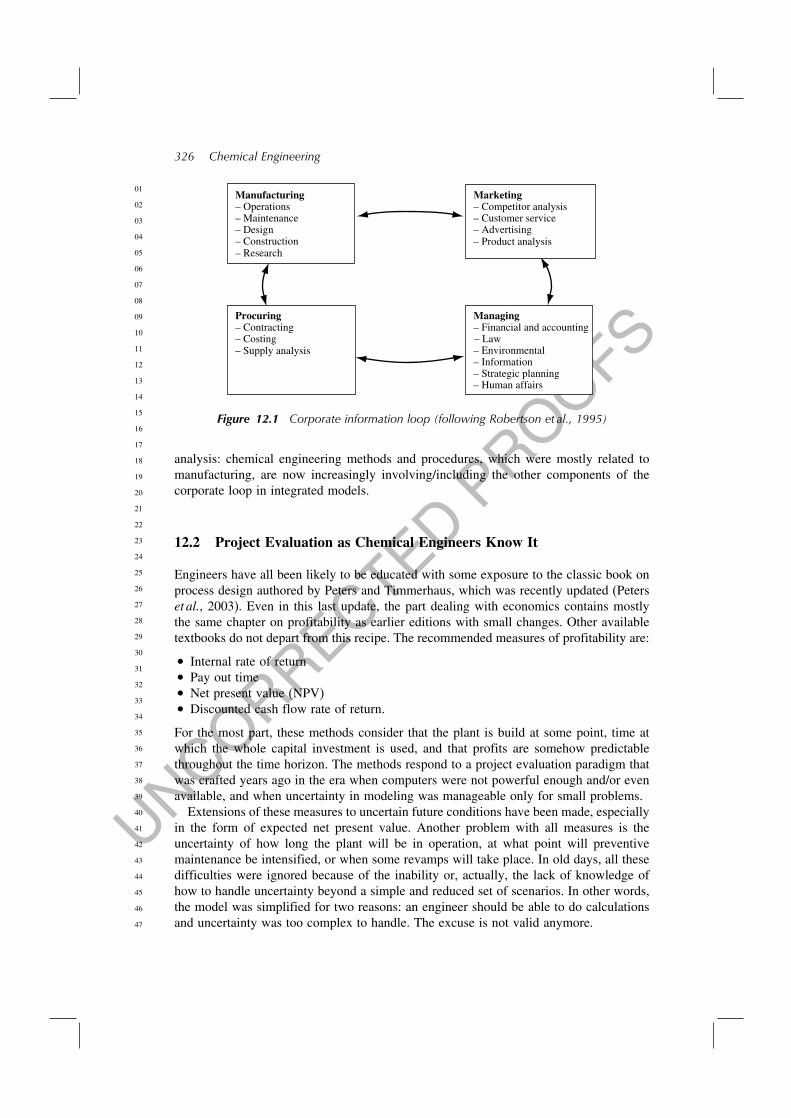
The answer to the above list of questions (which is by no means exhaustive) is slowlyand strongly emerging. The latest Eighth International Symposium on Process SystemsEngineering held in China (PSE 2003) had many of the above issues as the central theme,but there is substantial earlier pioneering work. For example, in an article mostly devotedto prepare us for the information technology (IT) age (now in full development), and itsimpact on corporate management, Robertson et al. (1995) argued about the lack of propercommunication in the corporate flow loop (Figure 12.1). They argue that the four majorcomponents of this loop (manufacturing, procuring, managing, and marketing) operatealmost as separate entities with minimal data sharing.

Notwithstanding the lack of data sharing, which will (or is being) corrected, the realissue is that the different elements of the loop also start to share the same goals andmethods, like Bunch and Iles (1998) argued. As in many examples illustrated in thefollowing text, decisions at the level of manufacturing, for example the schedule ofoperations, are influenced by the company’s cash position and are related to pricing,etc. This involves marketing, procuring, and manufacturing in the solution of the prob-lem. Corporate management, procuring, and marketing should also work together tosolve investment problems, etc. This is the nature of the challenge and the core of our

UNCORRECTED PROOFS

01

02

03

04

05

06

07

08

09

10

11

12

13

14

15

16

17

18

19

20

21

22

23

24

25

26

27

28

29

30

31

32

33

34

35

36

37

38

39

40

41

42

43

44

45

46

47


Procuring– Contracting– Costing– Supply analysis

Manufacturing– Operations– Maintenance– Design– Construction– Research

Managing– Financial and accounting– Law– Environmental– Information– Strategic planning– Human affairs

Marketing– Competitor analysis– Customer service– Advertising– Product analysis

Figure 12.1 Corporate information loop (following Robertson et al., 1995)

analysis: chemical engineering methods and procedures, which were mostly related tomanufacturing, are now increasingly involving/including the other components of thecorporate loop in integrated models.

12.2 Project Evaluation as Chemical Engineers Know It

Engineers have all been likely to be educated with some exposure to the classic book onprocess design authored by Peters and Timmerhaus, which was recently updated (Peterset al., 2003). Even in this last update, the part dealing with economics contains mostlythe same chapter on profitability as earlier editions with small changes. Other availabletextbooks do not depart from this recipe. The recommended measures of profitability are:

• Internal rate of return• Pay out time• Net present value (NPV)• Discounted cash flow rate of return.

For the most part, these methods consider that the plant is build at some point, time atwhich the whole capital investment is used, and that profits are somehow predictablethroughout the time horizon. The methods respond to a project evaluation paradigm thatwas crafted years ago in the era when computers were not powerful enough and/or evenavailable, and when uncertainty in modeling was manageable only for small problems.

Extensions of these measures to uncertain future conditions have been made, especiallyin the form of expected net present value. Another problem with all measures is theuncertainty of how long the plant will be in operation, at what point will preventivemaintenance be intensified, or when some revamps will take place. In old days, all thesedifficulties were ignored because of the inability or, actually, the lack of knowledge ofhow to handle uncertainty beyond a simple and reduced set of scenarios. In other words,the model was simplified for two reasons: an engineer should be able to do calculationsand uncertainty was too complex to handle. The excuse is not valid anymore.

UNCORRECTED PROOFS

01

02

03

04

05

06

07

08

09

10

11

12

13

14

15

16

17

18

19

20

21

22

23

24

25

26

27

28

29

30

31

32

33

34

35

36

37

38

39

40

41

42

43

44

45

46

47


Do not test

Test

High demandP = 60%

Low demandP = 60%

Launch

Launch

Do not launch

Do not launch

Figure 12.2 Example of a decision tree

Despite the aforementioned general tendency, uncertainty in project evaluations hasbeen handled for years in various forms. Various branches of engineering still use decisionmodels, trees, and payoff tables (McCray, 1975; Riggs, 1968; Gregory, 1988; Schuyler,2001). Decision trees are good tools as long as decisions are discrete (e.g. to build a plantor not, to delay construction or not, etc.). A typical tree for investment decision makingis illustrated next. Consider a company trying to decide if it wants to invest 5 million totest a product in the market, and if a test is positive, invest 50 million, or skip the test.A decision tree for this case is shown in Figure 12.2. In this decision tree, two types ofnodes typically exist, those associated with decisions (test or not test) and the outcomesor external conditions (high/low demand), to which probabilities are associated.

Thus, to build a decision tree, one needs to explicitly enumerate all possible scenariosand the responses (decisions) to such scenarios. However, ‘for some problems, ,a combinatorial explosion of branches makes calculations cumbersome or impractical’(Schuyler, 2001). One way that this problem is ameliorated (but not solved) is byintroducing Monte Carlo simulations at each node of the decision tree. However, thisdoes not address the problem of having to build the tree in the first place. In addition,trees are appropriate for the case where discrete decisions are made. Continuous decisionslike for example the size of the investment, or more specifically, the size of a productionplant, cannot be easily fit into decision trees without discretizing.

A separate paragraph needs to be devoted to dynamic programming (Bellman, 1957;Denardo, 1982). This technique is devoted to solve sequential decision making processes.It has been applied to resource allocation, inventory management, routing in networks,production control, etc. In many aspects this technique is equivalent to two-/multi-stage stochastic programming, with the added benefits that under certain conditions,some properties of the solutions (optimality conditions) are known and are helpful forthe solution procedure. In fact, under certain conditions, one can obtain the solutionrecursively, moving backwards from the last node to the first. The technique can beapplied to problems under uncertainty. There has been recently a revival of the usage ofthis technique in chemical engineering literature due fundamentally to the recent workof Professor Westerberg (Cheng et al., 2003, 2004).

By the late 1980s the engineering community had started to introduce two-stagestochastic programming (Birge and Louveaux, 1997) in problems like planning, schedul-ing, etc. (Iyer and Grossmann, 1998a; Liu and Sahinidis, 1996; Gupta and Maranas,2000, and many others). Two-stage stochastic programming is briefly outlined next usinglinear functions for simplicity. The dynamic programming approach is outlined brieflylater.

UNCORRECTED PROOFS

01

02

03

04

05

06

07

08

09

10

11

12

13

14

15

16

17

18

19

20

21

22

23

24

25

26

27

28

29

30

31

32

33

34

35

36

37

38

39

40

41

42

43

44

45

46

47


12.2.1 Two-Stage Stochastic Programming

Two features characterize these problems: the uncertainty in the problem data and thesequence of decisions. Several model parameters, especially those related to future events,are considered random variables with a certain probability distribution. In turn, somedecisions are taken at the planning stage, that is, before the uncertainty is revealed, whilea number of other decisions can only be made after the uncertain data become known. Thefirst decisions are called first-stage decisions and the decisions made after the uncertaintyis unveiled are called second-stage or recourse decisions, and the corresponding periodis called the second stage. Typically, first-stage decisions are structural and most ofthe time related to capital investment at the beginning of the project, while the second-stage decisions are often operational. However, some structural decisions correspondingto a future time can be considered as second-stage decisions. This kind of situation isformulated through the so-called multi-stage models, which are a natural extension ofthe two-stage case. Among the two-stage stochastic models, the expected value of thecost (or profit) resulting from optimally adapting the plan according to the realizationsof uncertain parameters is referred to as the recourse function. Thus, a problem is saidto have complete recourse if the recourse cost (or profit) for every possible uncertaintyrealization remains finite, independently of the nature of the first-stage decisions. In turn,if this statement is true only for the set of feasible first-stage decisions, the problem issaid to have relatively complete recourse (Birge and Louveaux, 1997). This conditionmeans that for every feasible first-stage decision, there is a way of adapting the plan tothe realization of uncertain parameters. The following literature covers the technique inmore detail: Infanger (1994), Kall and Wallace (1994), Higle and Sen (1996), Birge andLouveaux (1997), Marti and Kall (1998), and Uryasev and Pardalos (2001). In addition,Pistikopoulos and Ierapetritou (1995), Cheung and Powell (2000), Iyer and Grossmann(1998b), and Verweij et al. (2001) discuss solution techniques for these problems.

The general extensive form of a two-stage mixed-integer linear stochastic problem fora finite number of scenarios can be written as follows (Birge and Louveaux, 1997):Model SP:

Max EProfit =∑

s∈S

psqTs ys − cTx (12.1)

st

Ax = b (12.2)

Tsx+Wys = hs ∀s ∈ S (12.3)

x ≥ 0 x ∈ X ys ≥ 0 ∀s ∈ S (12.4)

In the above model, x represents the first-stage mixed-integer decision variables andys are the second-stage variables corresponding to scenario s, which has occurrenceprobability ps. The objective function is composed of the expectation of the profitgenerated from operations minus the cost of first-stage decisions (capital investment).The uncertain parameters in this model appear in the coefficients qs, the technologymatrix Ts, and in the independent term hs. When W , the recourse matrix, is deterministicthe problem is called to be of fixed recourse. Cases where W is not fixed are found forexample in portfolio optimization when the interest rates are uncertain (Dupacova andRömisch, 1998).

UNCORRECTED PROOFS

01

02

03

04

05

06

07

08

09

10

11

12

13

14

15

16

17

18

19

20

21

22

23

24

25

26

27

28

29

30

31

32

33

34

35

36

37

38

39

40

41

42

43

44

45

46

47


It is worth noticing that decision trees are in fact a particular case of two-stageprogramming. In other words, one can code through rules (mathematical in this case)the same decisions one make in the tree explicitly, but in two-stage programming, onecan also add logical constraints, if-the-else rules, etc., so there is no need for explicitenumeration of all options.

Aside from the issue of the plant life and the possible future upgrades, which complicatethe modeling, there is yet another very important difficulty with these methods: themodels are isolated from considering the size of the company, the health of its finances,even the temporary lack of liquidity or the abundance thereof as it was pointed outabove. Take, for example, the simple question: Should the project be started this year,next year, or two years down the road? The answer relies on forecasting of course, andthe choice can be modeled using current two-stage stochastic programming methods, butmaximizing the above measures is not proper most of the time, as the answer is not thesame if the project is undertaken by a big corporation or a small company.

One important point to make is that before any treatment of risk or uncertainty, a soliddeterministic model needs to be developed.

Summarizing: Chemical engineers have understood uncertainty and flexibility and haveincorporated it within a two (multi)-stage process decision optimization models. In doingso, Chemical Engineers are not embracing the use of decision trees, which, as claimed,are a particular case of the former. Integration of financial indicators other than financialrisk as well as strategic planning as a whole has barely started.

12.3 Project Evaluation the Way Economistsand Financiers Practice It

One learns from books on financial management (Keown et al., 2002, Smart et al., 2004)that maximization of shareholder wealth, that is, maximization of the price of the existingcommon stock, is the real goal of a firm, not just maximization of profit as engineers aretrained to think. Some alternative form of maximizing dividends should be substitutedif the company is non-publicly owned. They claim that such a goal also benefits societybecause ‘scarce resources will be directed to their most productive use by businessescompeting to create wealth’. Finance management also teaches that several other issuesare of importance for that goal, namely:

• risk management, that is, its eventual reduction;• risk diversification, that is, risky projects can be combined with other less risky ones

in a balanced portfolio;• cash flow management includes borrowing, raising investor’s money, and also buying

and selling securities;• liquidity of the firm (ratio of assets to liabilities) and available cash, which affects

investment and operating decisions;

among others. To deal with risk, they mostly measure it using variability (or volatility),which is incorrect in almost all engineering project cases, as it is explained later. Theydiversify by adding stocks to the portfolio.

UNCORRECTED PROOFS

01

02

03

04

05

06

07

08

09

10

11

12

13

14

15

16

17

18

19

20

21

22

23

24

25

26

27

28

29

30

31

32

33

34

35

36

37

38

39

40

41

42

43

44

45

46

47


12.3.1 Profit Maximization

Capital budgeting, the process through which the company analyzes future cash inflowsand outflows, is performed using concepts that are extensions of the tools engineersknow.

The firm cost of capital, which is the hurdle rate that an investment must achieve beforeit increases shareholder value, is one key aspect of these decisions that the engineers haveoverlooked. Such cost of capital is measured typically by the firm’s weighted averagecost of capital (WACC) rate kWACC. For example, a firm that uses only debt and commonequity to finance its projects, this rate is given by:

kWACC = After tax cost of debt×+ Cost of equity1− (12.5)

where is the portion of debt that one is financing, the cost of debt is that rate paid forborrowed money, and the cost of equity is the rate that shareholders expect to get fromthe cash retained in the business and used for this project. The latter rate is larger thanthe former, of course.

In practice kWACC is more complex to calculate because there are several debts incurredat different times and they require common equity as well as preferred equity. In addition,new capital may be raised through new stock offerings. Finally, one is faced with theproblem of calculating a return of a project that has multiple decisions at different times,with uneven and uncertain revenues. Clearly, this simple formula needs some expansion,to add the complexities of projects containing multiple first- and second-stage decisionsthrough time.

Financial management also suggests the alternative that the appropriate discount rateto evaluate the NPV of a project is the weighted average cost of capital, based on oneimportant assumption that the risk profile of the firm is constant over time. In addition,this is true only when the project carries the same risk as the whole firm. When that isnot true, which is most of the time, finance management has more elaborate answers,like managerial decisions that ‘shape’ the risk.

They also manage projects for market value added (MVA). The free cash flow modelprovides the firm value:

Firm value =∑

i

Free cash flowi

1+kWACCi+ Terminal value

1+kWACCn(12.6)

where the summation is extended over the period of n periods of planning. This expressionuses kWACC and refers to the whole company. The firm value is used to get the marketvalue added of the investment.

Market value added = Firm value − Investment (12.7)

which is a formula very similar to the net present value engineers use for projects. Infact, the only difference is the value of the hurdle rate. Because the formula is a measureof the total wealth created by a firm at a given time, extending over a long time horizon,financial experts recommend the use of a shorter term measure, the economic value added(EVA) for period t.

EVAt = Net profitt −kWACCInvested capital (12.8)

UNCORRECTED PROOFS

01

02

03

04

05

06

07

08

09

10

11

12

13

14

15

16

17

18

19

20

21

22

23

24

25

26

27

28

29

30

31

32

33

34

35

36

37

38

39

40

41

42

43

44

45

46

47


where the net profit is computed after taxes. Thus, the MVA is the present value of allfuture EVA. Quite clearly, finance experts warn, managing for an increased EVA at anygiven time may lead to a non-optimal MVA.

In turn, the shareholder value can be obtained as follows: The firm value is the sum ofdebt value plus equity value. Then, if one knows the long-term interest-bearing liabilities,one has the debt value. Then one can obtain the shareholder value,

Shareholder value = Equity valueNumber of shares

= Firm value −Debt valueNumber of shares

(12.9)

In principle, as noted above, the shareholder value is what one wants to maximize. This iswhat is true for the whole company and therefore implies one has to consider all projectsat the same time. Thus, one can write

Shareholder value = Equity valueNumber of shares

=∑

pFirm valuepxp−Debt valuepxp

Number of shares(12.10)

where the summation is extended over different projects the firm is pursuing or consid-ering pursuing and xp is the vector of first-stage (‘here and now’) decisions to be made.Thus, if the projects are generating similar equity value, no simplification is possible anddecisions have to be made simultaneously for all projects. Hopefully, procedures thatwill do this interactively, that is, change the decisions of all projects at the same time,will be developed.

However, which shareholder value does one want to maximize? The one correspondingto next quarter company report, or a combination of shareholder values in different pointsin the future? In other words, is there such thing as an optimal investment and operatingstrategy/path? This looks like an optimal control problem!

And then, there is the dividend policy. Is it possible that this should be decided togetherwith and not independently from the specific project first-stage variables?

The ‘here and now’ decisions xp involve several technical choices of the processesthemselves (catalysts, technologies, etc.) which require detailed modeling and also someother ‘value drivers’, like advertisement to increase sales, alliances to penetrate markets,investment in R&D, company acquisition, cost-control programs, inventory control, con-trol of the customer paying cycles (a longer list is given by Keown et al., 2002). Most ofthese ‘knobs and controls’ are called second-stage (‘wait and see’) decisions, but manyare also first-stage decisions.

The literature on strategic planning (Hax and Majluf, 1984) has models that deal directlywith shareholder value. They use different models (market to book values, profitabilitymatrices, etc.) to obtain corporate market value, which take into account the companyreinvestment policy, dividend payments, etc. One cannot help also mention some classicand highly mathematical models from game theory and other analytical approaches, someof which are discussed elegantly by Debreu (1959) and Danthine and Donaldson (2002).

A brief glance at the literature tells that economists are not yet so keen on using two-stage stochastic models. They understand, of course, the concept of options in projects,but many are still ‘locked’ to the use of point measures like NPV and decision trees(De Reyck et al., 2001).

UNCORRECTED PROOFS

01

02

03

04

05

06

07

08

09

10

11

12

13

14

15

16

17

18

19

20

21

22

23

24

25

26

27

28

29

30

31

32

33

34

35

36

37

38

39

40

41

42

43

44

45

46

47


Finally, some of the financial ratios that are waiting to be embraced by engineeringmodels are:

• Liquidity ratios

– Current ratio = current assets/current liabilities– Acid test or quick ratio = (current asset inventories)/current liabilities– Average collection period: accounts receivable/daily credit sales– Accounts receivable turnover = credit sales/accounts receivable– Inventory turnover = costs of goods sold/inventory

• Operating profitability ratios

– Operating income return on investment = income/total assets– Operating profit margin = income/sales– Total assert turnover = sales/ total assets– Accounts receivable turnover = sales/accounts receivable– Fixed assets turnover = sales/net fixed assets

• Financial ratios

– Debt ratio = total debt/total assets– Times interests earned = operating income/interest expense– Return on equity = net income/common equity

While all these indicators focus on different aspects of the enterprise, they should be atleast used as constraints in engineering models.

It is therefore imperative that engineers incorporate these measures and objectives inproject evaluation, when and if, of course, decisions at the technical level have an impacton the outcome. In other words, how much of the project is financed by equity is adecision to make together with the technical decisions about size and timing of everyproject and the technical decisions of the project itself, like the selection of technologies,catalysts, etc. This last aspect is what makes the integration a must!

12.3.2 Risk Management

The other major component influencing business decisions is risk. First, one needs todistinguish business risk from financial risk.

Business risk is measured by the non-dimensional ratio of variability (standard devia-tion) to expected profit before taxes and interest (Keown et al., 2002; Smart et al., 2004).Thus the same variability associated with a larger profit represents less business risk.Thus, one can use this ratio to compare two investments, but when it comes to managingrisk for one investment, the objective seems to be the usual, maximize profit and reducevariability. As it will be discussed later in greater detail, these are conflicting goals.Measures to reduce business risk include product diversification, reduction of fixed costs,managing competition, etc. More specifically, the change in product price and fixed costsis studied through the degree of operating leverage (DOL) defined in various forms, onebeing the ratio of revenue before fixed costs to earnings before interest and taxes (EBIT).

Engineers have not yet caught up in relating these concepts with their models. As usual,the mix includes some second-stage decisions, but most of them are first-stage ‘hereand now’ decisions. Modeling through two-stage stochastic programming and including

UNCORRECTED PROOFS

01

02

03

04

05

06

07

08

09

10

11

12

13

14

15

16

17

18

19

20

21

22

23

24

25

26

27

28

29

30

31

32

33

34

35

36

37

38

39

40

41

42

43

44

45

46

47


technical decisions in this modeling is the right answer. Some of the aspects of thismodeling are discussed below.

Financial risk is in some cases defined as the ‘additional variability in earnings and the additional chance of insolvency caused by the use of financial leverage’(Keown et al., 2002). In turn, the financial leverage is the amount of assets of the firmbeing financed by securities bearing a fixed or limited rate of return. Thus, the degree offinancial leverage (DFL) is defined as the ratio of EBIT to the difference of EBIT andthe total interest expense I , that is,

DFL = EBITx

EBITx− Ix(12.11)

In other words, business and financial risk differ fundamentally in that one considersinterest paid and the other does not. Both are considered related to variability. As it isshown later, the claim is that this is the wrong concept to use in many cases.

Another very popular definition of risk is through the risk premium or beta. This isdefined as the slope of the curve that gives market returns as a function of S&P 500Index returns; in other words, comparing how the investment compares with the market.The concept of ‘beta’ (the slope of the curve) is part of the capital asset pricing model(CAPM) proposed by Lintner (1969) and Sharpe (1970), which intends to incorporaterisk into valuation of portfolios and it can also be viewed as the increase in expectedreturn in exchange for a given increase in variance. However, this concept seems to applyto building stock portfolios more than to technical projects within a company.

Financial risk is also assessed through point measures like risk-adjusted return ofcapital (RAROC), risk-adjusted net present value (RPV), Sharpe ratio (Sharpe, 1966). Itis unclear if these point measures are proper ways of assessing risk, much less managingit, in engineering projects. This point is expanded below.

Economists also consider risk as ‘multidimensional’ (Dahl et al., 1993). They havecoined names for a variety of risks. Some of these, applied mostly to stocks, bonds, andother purely financial instruments, are market risk (related to the CAPM model and theabove described parameter ‘beta’), volatility risk (applied to options, primarily), currencyrisk, credit risk, liquidity risk, residual risk, inventory risk, etc.

The managing of net working capital is used by finance experts to manage risk. Theworking capital is the total assets of the firm that can be converted to cash in a one-yearperiod. In turn, the net working capital is the difference between assets and liabilities.Thus increasing the net working capital reduces the chance of low liquidity (lack of cashor ability to convert assets into cash to pay bills in time). This is considered as short-termrisk. Several strategies are suggested to maintain an appropriate level of working capital(Finnerty, 1993).

A separate consideration needs to be made for inventory, which in principle is used tobe able to uncouple procuring from manufacturing and sales. In this regard it is mostlyconsidered as a risk hedging strategy that increases costs. Finally, contracts, especiallyoption contracts and futures, are other risk hedging tools.

Recently, risk started to be defined in terms of another point measure introducedby J.P. Morgan, value at risk or VaR (Jorion, 2000). This is defined as the differencebetween the expected profit and the profit corresponding to 5% cumulative probability.Many other ‘mean-risk’ models use measures like tail value at risk, weighted mean

UNCORRECTED PROOFS

01

02

03

04

05

06

07

08

09

10

11

12

13

14

15

16

17

18

19

20

21

22

23

24

25

26

27

28

29

30

31

32

33

34

35

36

37

38

39

40

41

42

43

44

45

46

47


455

555

655

755

855

955

455 555 655 755 855

Risk averse utility

Risk taker’s utility

Util

ity v

alue

Real value

Figure 12.3 Utility functions

deviation form a quantile, and the tail Gini mean difference (reviewed by Ogryczak andRuszcynski, 2002), to name a few.

More advanced material (Berger, 1980; Gregory, 1988; Danthine and Donaldson, 2002)proposes the use of expected utility theory to assess risks. This theory proposes to assigna value (different from money) to each economic outcome. Figure 12.3 illustrates theutility function of a risk-averse decision maker, who values (in relative terms) smalloutcomes more than large outcomes. It also shows the utility function of a risk takerwho places more value in higher outcomes. In most cases, the utility curve is constructedin a somehow arbitrary manner, that is, taking two extreme outcomes and assigning avalue of 0 to the less valued and the value of 1 to the most valued one. Then there areprocedures that pick intermediate outcomes and assign a value to them until the curve isconstructed.

This theory leads to the definition of loss functions as the negative utility values, whichare used to define and manipulate risk (Berger, 1980). To do this, a decision rule must bedefined. Thus, risk is defined as the expected loss for that particular decision rule. This,in turn, leads to the comparison of decision rules. Engineering literature contains somereference to this theory. As it is discussed below, expected utility has a lot of potentialas decision making tool. All that is needed is to start putting it in the context of theemerging two-stage stochastic modeling.

The important thing one learns from the review of basic financing is as follows:

1) The majority of the tools proposed are deterministic, although some can be extendedto expectations on profit distributions and therefore decision trees are presented asadvanced material in introductory finance books. Quite clearly, one would benefitfrom using two-stage stochastic programming instead.

2) Risk is considered a univariate numerical measure like variability or value at risk(VaR), which is the difference between the project expected outcome and the profitcorresponding to (typically) 5% cumulative probability. Opportunities at high profitlevels are rarely discussed or considered.

3) Financiers only know how to evaluate a project. They can manipulate it on thefinancial side, but they cannot manipulate it in its technological details because they

UNCORRECTED PROOFS

01

02

03

04

05

06

07

08

09

10

11

12

13

14

15

16

17

18

19

20

21

22

23

24

25

26

27

28

29

30

31

32

33

34

35

36

37

38

39

40

41

42

43

44

45

46

47


need engineering expertise for it. This is the Achilles heel of their activity. Engineers,in turn, cannot easily take into account the complexity of finances. Both need eachother more than ever.

12.4 Latest Progress of Chemical Engineering Models

Decision making is an old branch of management sciences, a discipline that has alwayshad some overlap with engineering, especially industrial engineering. Some classicalbooks on the subject (Riggs, 1968; Gregory, 1988; Bellman, 1957) review some of thedifferent techniques, namely:

• resource allocation (assignment, transportation);• scheduling (man–machine charts, Gantt charts, critical path scheduling, etc.);• dynamic programming (Bellman, 1957; Denardo, 1982);• risk (reviewed in more detail in the next section) through the use of decision trees,

regret tables, and utility theory.

Notwithstanding the value of all these techniques, the new emerging procedures relyheavily on two-stage stochastic programming and some revival of dynamic programming.It is argued here that several techniques, like decision trees and utility theory, are specialcases of two-stage stochastic programming. Others claim the same when advocating thedynamic programming approach (Cheng et al., 2003, 2004). They proposed to modeldecision making as a multiobjective Markov decision process.

For example, in recent years, the integration of batch plant scheduling with economicactivities belonging to procuring and marketing has been pioneered by the books byPuigjaner et al. (1999, 2000), which contain full chapters on financial management inbatch plants where something similar to the corporate information loop (Figure 12.1), asviewed by engineers and economists, is discussed. They discuss the notion of enterprisewide resource management systems (ERM), one step above enterprise resource planning(ERP). They outline the cycle of operations involving cash flow and working capital, themanagement of liquidity, the relationships to business planning, etc. as it relates mostlyto batch plants. They even raise the attention to the role of pricing theory and discussthe intertwining of these concepts with existing batch plant scheduling models. Thesesummary descriptions of the role of cash and finances in the context of batch plantsare the seeds of the mathematical models that have been proposed afterwards. Extensivework was also performed by many other authors in a variety of journal articles. A partial(clearly incomplete) list of recent work directly related to the integration of processsystems engineering and economic/financial tools is the following:

• Investment planning (Sahinidis et al., 1989; Liu and Sahinidis, 1996; McDonald andKarimi, 1997; Bok et al., 1998; Iyer and Grossmann, 1998a; Ahmed and Sahinidis,2000a, Cheng et al., 2003, 2004).

• Operations planning (Ierapetritou et al., 1994; Ierapetritou and Pistikopoulos, 1994;Pistikopoulos and Ierapetritou, 1995; Iyer and Grossmann, 1998a; Lee and Malone,2001; Lin et al., 2002; Mendez et al., 2000; McDonald, 2002; Maravelias andGrossmann, 2003; Jackson and Grossmann, 2003; Mendez and Cerdá, 2003).

UNCORRECTED PROOFS

01

02

03

04

05

06

07

08

09

10

11

12

13

14

15

16

17

18

19

20

21

22

23

24

25

26

27

28

29

30

31

32

33

34

35

36

37

38

39

40

41

42

43

44

45

46

47


• Refinery operations planning (Shah, 1996; Lee et al., 1996; Zhang et al., 2001; Pintoet al., 2000; Wenkai et al., 2002; Julka et al., 2002b; Jia et al., 2003; Joly and Pinto,2003; Reddy et al., 2004; Lababidi et al., 2004; Moro and Pinto, 2004).

• Design of batch plants under uncertainty (Subrahmanyan et al., 1994; Petkov andMaranas, 1997).

• Integration of batch plant scheduling and planning and cash management models(Badell et al., 2004; Badell and Puigjaner, 1998, 2001a,b; Romero et al., 2003a,b).

• Integration of batch scheduling with pricing models (Guillén et al., 2003a).• Integration of batch plant scheduling and customer satisfaction goals (Guillén et al.,

2003b).• Technology selection and management of R&D (Ahmed and Sahinidis, 2000b;

Subramanian et al., 2000).• Supply chain design and operations (Wilkinson et al., 1996; Shah, 1998; Bok et al.,

2000, Perea-Lopez et al., 2000; Bose and Pekny, 2000; Gupta and Maranas, 2000;Gupta et. al., 2000; Tsiakis et al., 2001; Julka et al., 2002a,b; Singhvi and Shenoy,2002; Perea-Lopez et al., 2003; Mele et al., 2003; Espuña et al., 2003; Neiro and Pinto,2003).

• Agent-based process systems engineering (Julka et al., 2002a,b; Siirola et al., 2003).• Financial risk through the use of a variety of approaches and in several applications

(Applequist et al., 2000; Gupta and Maranas, 2003a; Mele et al., 2003; Barbaro andBagajewicz, 2003, 2004a,b; Wendt et al., 2002; Orcun et al., 2002).

• New product development (Schmidt and Grossmann, 1996; Blau and Sinclair, 2001;Blau et al., 2000).

• Product portfolios in the pharmaceutical industry (Rotstein et al., 1999).• Options trading and real options (Rogers et al., 2002, 2003; Gupta and Maranas, 2003b,

2004).• Transfer prices in supply chain (Gjerdrum et al., 2001).• Oil drilling (Iyer et al., 1998; Van den Heever et al., 2000, 2001; Van den Heever and

Grossmann, 2000; Ortiz-Gómez et al., 2002)• Supply chain in the pharmaceutical industry (Papageorgiou et al., 2001; Levis and

Papageorgiou, 2003).• Process synthesis using value added as an objective function (Umeda, 2004). This

chapter revisits dynamic programming approaches.

The rest of this chapter concentrates on discussing some aspects of the integration thathave received attention by engineers, namely,

• financial risk• effect of inventories• regular, future, and option contracts• budgeting• pricing• consumer satisfaction.

Some work calling for the integration of other disciplines and the role of the recentproduct engineering and the chemical supply chain key ideas in the integration withfinances is also mentioned.

UNCORRECTED PROOFS

01

02

03

04

05

06

07

08

09

10

11

12

13

14

15

16

17

18

19

20

21

22

23

24

25

26

27

28

29

30

31

32

33

34

35

36

37

38

39

40

41

42

43

44

45

46

47


12.5 Financial Risk Management

12.5.1 Definition of Risk

There are various definitions of risk in the engineering literature, most of them rooted inthe finance field, of course.

A good measure of risk has to take into account different risk preferences and thereforeone may encounter different measures for different applications or attitudes toward risk.The second property that a risk measure should have is that when it focuses on particularoutcomes, say low profit outcomes that want to be averted as in the figure above, onewould like to also have information about the rest of the profit distribution. Particularly,when one compares one project to another, one would like to see what is that one losesin other portions of the spectrum as compared to what one gains averting risk.

Some of these alternative measures that have been proposed are now reviewed:

• Variability: That is, standard deviation of the profit distribution. This is the mostcommon assumption used in the non-specialized financial literature, where invest-ment portfolios (stocks primarily) are considered. Mulvey et al. (1995) introduced theconcept of robustness as the property of a solution for which the objective value forany realized scenario remains ‘close’ to the expected objective value over all possi-ble scenarios and used the variance of the cost as a ‘measure’ of the robustness ofthe plan, i.e. less variance corresponds to higher robustness. It is obvious that thesmaller the variability, the less negative deviation from the mean. But it also impliessmaller variability on the optimistic side. Thus, either the distribution is symmetric(or this is assumed) or one does not care about the optimistic side. This is the specificassumption of stock portfolio optimization, but it is known not to be correct for othertype of investments, especially multi-year ones (Smart et al., 2004). Thus, the use ofvariability as a measure of risk is being slowly displaced by engineers (not necessarilyby the finance community) in favor of other measures. Nonetheless, it is still beingused. Tan (2002), for example, provides means to reduce variability by using capacityoptions in manufacturing. It has the added disadvantage that it is nonlinear.

• Cumulative probability for a given aspiration level: This is the correct way of definingrisk when one wants to reduce its measure to a single number because unlike varianceit deals with the pessimistic side of the distribution only. Consider a project definedby x. Risk is then defined by

Riskx = PProfitx ≤ (12.12)

where Profit(x) is the actual profit, showed in Figure 12.4 as the shaded area. Thisdefinition has been used by the petroleum industry for years (McCray, 1975). In theprocess systems literature this definition was used by Rodera and Bagajewicz (2000),Barbaro and Bagajewicz (2003, 2004a), and Gupta and Maranas (2003a). Figure 12.5depicts a cumulative distribution curve, which also represents risk as a function of allaspiration levels. This is the preferred representation because, as it is discussed later,one can best manage risk using it.

• Downside risk: This measure, introduced by Eppen et al. (1989) in the frameworkof capacity planning for the automobile industry, is an alternative and useful way of

UNCORRECTED PROOFS

01

02

03

04

05

06

07

08

09

10

11

12

13

14

15

16

17

18

19

20

21

22

23

24

25

26

27

28

29

30

31

32

33

34

35

36

37

38

39

40

41

42

43

44

45

46

47


0.00

0.02

0.04

0.06

0.08

0.10

0.12

0.14

0.16

0.18

0.20

Profit

Prob

abili

ty

Cumulative probability= Risk(x,Ω)

Ω ξ

Figure 12.4 Definition of risk. Discrete case

0.0

0.1

0.2

0.3

0.4

0.5

0.6

0.7

0.8

0.9

1.0

Profit

Ris

k

x fixed

Figure 12.5 Risk curve, continuous case

measuring risk using the concept of currency. Consider the positive deviation from aprofit target for design x x, defined as follows:

x =

−Profitx If Profitx <

0 Otherwise(12.13)

UNCORRECTED PROOFS

01

02

03

04

05

06

07

08

09

10

11

12

13

14

15

16

17

18

19

20

21

22

23

24

25

26

27

28

29

30

31

32

33

34

35

36

37

38

39

40

41

42

43

44

45

46

47


0.0

0.1

0.2

0.3

0.4

0.5

0.6

0.7

0.8

0.9

1.0

Profit ξ

Ris

k(x,

ξ)x fixed

Area = DRisk(x,Ω)

Ω

Figure 12.6 Interpretation of downside risk

Downside risk is then defined as the expectation of x, that is, DRiskx =E x. This form has been very useful computationally to identify process alter-natives with lower risk, as it is discussed below. Barbaro and Bagajewicz (2003,2004a) proved that downside risk is just an integral of the risk curve, as shown inFigure 12.6. Moreover, they proved that downside risk is not monotone with risk, thatis, two designs can have the same risk for some aspiration level, but different downsiderisk. Moreover, projects with higher risk than others can exhibit lower downside risk.Therefore, minimizing one does not imply minimizing the other. However, this mea-sure has several computational advantages and was used to generate solutions whererisk is managed using goal programming (Barbaro and Bagajewicz, 2003, 2004a).Gupta and Maranas (2003a) discuss these measures (risk and downside risk) as well.

• Upper partial mean: It is proposed by Ahmed and Sahinidis (1998). It is definedas the expectation of positive deviation from the mean, that is, UPMx = Ex,where x is defined the same way as x, but using EProfitx instead.In other words, the UPM is defined as the expectation of the positive deviationof the second-stage profit. The UPM is a linear and asymmetric index since onlyprofits that are below the expected value are measured. However, in the context ofrisk management at the design stage, this measure cannot be used because it canunderestimate the second-stage profit by not choosing optimal second-stage policies.Indeed, because of the way the UPM is defined, a solution may falsely reduce itsvariability just by not choosing optimal second-stage decisions. This is discussed indetail by Takriti and Ahmed (2003), who present sufficient conditions for a measureof a robust optimization to assure that the solutions are optimal (i.e. not stochasticallydominated by others). For these reasons, downside risk is preferred, simply becausethe expectation of positive deviation is done with respect to a fixed target () and notthe changing profit expectation.

• Value at risk (VaR): It (discussed in detail by Jorion, 2000) was introduced byJ.P. Morgan (Guldimann, 2000) and is defined as the expected loss for a certain

UNCORRECTED PROOFS

01

02

03

04

05

06

07

08

09

10

11

12

13

14

15

16

17

18

19

20

21

22

23

24

25

26

27

28

29

30

31

32

33

34

35

36

37

38

39

40

41

42

43

44

45

46

47


confidence level usually set at 5% (Linsmeier and Pearson, 2000). A more generaldefinition of VaR is given by the difference between the mean value of the profit andthe profit value corresponding to the p-quantile. For instance, a portfolio that has anormal profit distribution with zero mean and variance , VaR is given by zp wherezp is the number of standard deviations corresponding to the p-quantile of the profitdistribution. Most of the uses of VaR are concentrated on applications where the profitprobability distribution is assumed to follow a known symmetric distribution (usuallythe normal) so that it can be calculated analytically. The relationship between VaRand Risk is generalized as follows (Barbaro and Bagajewicz, 2004a):

VaRxp = EProfitx−Risk−1xp (12.14)

where p is the confidence level related to profit , that is, p = Riskx. Noticethat VaR requires the computation of the inverse function of Risk. Moreover, sinceRisk is a monotonically increasing function of , one can see from equation 12.14that VaR is a monotonically decreasing function of p.

While computing VaR as a post-optimization measure of risk is a simple task anddoes not require any assumptions on the profit distribution, it poses some difficultieswhen one attempts to use it in design models that manage risk. Given the computationalshortcomings, it is more convenient to use VaR as a risk indicator, only because ofits popularity in financial circles.

Finally, sometimes the risks of low liquidity measured by the cash flow at risk(CFAR) are more important than the value at risk (Shimko, 1998).

Companies that operate with risky projects identify VaR or similar measures directlywith potential liability, and they would hold this amount of cash through the life of aproject, or part of it.

• Downside expected profit (DEP): For a confidence level p (Barbaro and Bagajewicz,2004a), it is defined formally as the expectation of profit below a target correspondingto a certain level of risk p, that is, DEPxp = Ex, where

x =

Profitx If Profitx ≤

0 Otherwise(12.15)

and = Risk−1xp. Plotting DEP as a function of the risk is revealing because atlow risk values some feasible solutions may exhibit larger risk adjusted present value.The relationship between DEP, risk, and downside risk is

DEPxp =∫

−fx d = Riskx−DRiskx (12.16)

where fx is the profit distribution.• Regret analysis (Riggs, 1968): It is an old tool from decision theory that has been used

in a variety of ways to assess and manage risk (Sengupta, 1972; Modiano, 1987). Itsuse as a constraint in the context of optimization under uncertainty and aiming at themanaging of financial risk has been suggested by Ierapetritou and Pistikopoulos (1994).The traditional way of doing regret analysis requires the presence of a table ofprofits for different designs under all possible scenarios. One way to generate such

UNCORRECTED PROOFS

01

02

03

04

05

06

07

08

09

10

11

12

13

14

15

16

17

18

19

20

21

22

23

24

25

26

27

28

29

30

31

32

33

34

35

36

37

38

39

40

41

42

43

44

45

46

47


a table is to use the sampling average algorithm (Verweij et al., 2001) to solve adeterministic design, scheduling and/or planning model for several scenarios, one ata time or a certain number at a time, to obtain several designs (characterized byfirst-stage variables). The next step is to fix these first-stage variables to the valuesobtained and solve the model to obtain the profit of that design under every otherscenario. The different criteria to choose the preferred solution are as follows:

– The maximum average criterion states that one should choose the design thatperforms best as an average for all scenarios. This is equivalent to choosing thesolution with best ENPV.

– The maximax criterion suggests to choose the design that has the highest profitvalue in the profit table. This represents an optimistic decision in which all the badscenarios are ignored in favor of a single good scenario.

– The maximin criterion states that the design that performs best under the worst con-ditions is chosen. This is equivalent to identifying the worst-case value (minimumover all scenarios) for each design and choosing the design with the best worst-casevalue (or the maximum–minimum).

Aseeri and Bagajewicz (2004) showed that none of these strategies can guarantee theidentification of the best risk-reduced solutions, although in many instances they canbe used to identify promising and good solutions. For example, Bonfill et al. (2004)used the maximization of the worst case as means to obtain solutions that reduce riskat low expectations.

• Chance constraints (Charnes and Cooper, 1959): In essence, chance expressions arenot other than risk, as defined above, but usually applied to outcomes other than costor profit. Vice versa, financial risk can be thought of as a chance expression applied toprofit. Many authors (Orcun et al., 2002; Wendt et al., 2002) use chance expressionsby evaluating the probability that a design or a system can meet a certain uncertainparameter. Typical chance constraints have been used in scheduling of plant operationsto assess the probabilities of meeting certain levels of demand. Aseeri and Bagajewicz(2004) showed that this approach is less efficient than straight risk curve analysis andis in fact a special case of it. For example, a chance constraint for the production, e.g.Production ≤ Demand, should be replaced by Production ≤ F−11 −, where F isthe cumulative distribution for the demand and is the chosen confidence level. Buta model with these types of constraints is just one instance of a sampling algorithm.Thus, the approach of using chance constraints is a subset of the sampling averagealgorithm discussed above.

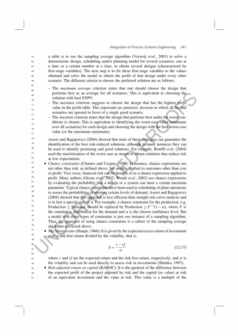
• The Sharpe ratio (Sharpe, 1966): It is given by the expected excess return of investmentover a risk-free return divided by the volatility, that is,

S = r − rf

(12.17)

where r and rf are the expected return and the risk-free return, respectively, and isthe volatility and can be used directly to assess risk in investments (Shimko, 1997).

• Risk-adjusted return on capital (RAROC): It is the quotient of the difference betweenthe expected profit of the project adjusted by risk and the capital (or value) at riskof an equivalent investment and the value at risk. This value is a multiple of the

UNCORRECTED PROOFS

01

02

03

04

05

06

07

08

09

10

11

12

13

14

15

16

17

18

19

20

21

22

23

24

25

26

27

28

29

30

31

32

33

34

35

36

37

38

39

40

41

42

43

44

45

46

47


Sharpe ratio in portfolio optimization, although this assertion is only valid for sym-metric distributions. This particular measure has not been used in two-stage stochasticengineering models to manage risk. This is not preferred because, as explained below,it is better to depart from single valued measures looking at the whole risk curvebehavior instead.

• Certainty equivalent approach (Keown et al., 2002): In this approach a certaintyequivalent is defined. This equivalent is the amount of cash required with certainty tomake the decision maker indifferent between this sum and a particular uncertain orrisky sum. This allows a new definition of net present value by replacing the uncertaincash flows by their certain equivalent and discounting them using a risk-free interestrate.

• Risk premium: Applequist et al. (2000) suggest benchmarking new investments againstthe historical risk premium mark. Thus, they propose a two-objective problem, wherethe expected net present value and the risk premium are both maximized. The tech-nique relies on using the variance as a measure of variability and therefore it penal-izes/rewards scenarios at both sides of the mean equally, which is the same limitationthat is discussed above.

• Risk-adjusted NPV (RPV) (Keown et al., 2001): This is defined as the net presentvalue calculated using a risk-adjusted rate of return instead of the normal return raterequired to approve a project. However, Shimko (2001) suggests a slightly differentdefinition where the value of a project is made up of two parts, one form the part ‘notat risk’ discounted using the risk-free return rate, and the part ‘at risk’ discounted atthe fully loaded cash plus risk cost.

• Real option valuation (ROV): Recently, Gupta and Maranas (2004) revisited a real-option-based concept to project evaluation and risk management. This frameworkprovides an entirely different approach to NPV-based models. The method relies onthe arbitrage-free pricing principle and risk neutral valuation. Reconciliation betweenthis approach and the above-described risk definitions is warranted.

• Other advances theories: Risk evaluation and its management continue to be anobject of research. For example, Jia and Dyer (1995) propose a method to weigh risk(defined through the variance and assuming symmetry) against value. These modelsare consistent with expected utility theory.

• More generally, some define risk as just the probability of an adverse economicevent and associate these adverse effects with something other than pessimistic profitlevels (Blau and Sinclair, 2001). For example, Blau et al. (2000) when analyzing drugdevelopment define risk as the probability of having more candidates in the pipelinethan available resources, which would result in delays in product launching. Whileall these are valid risk analyses, they are nonetheless, simplifications that one needsto remember one is doing. The ultimate risk analysis stems from the financial riskcurve based on profit of the whole enterprise, as will be explored in more detail inthe following text.

Fortunately, computers are available everywhere these days and tools to handle uncer-tainty and risk are also available: @Risk (Palisade http://www.palisade.com), CrystalBall (Decision Engineering, http://www.crystalball.com; Risk Analyzer (Macro Systems,http://www.macrosysinc.com/ ), Risk+(C/S Solutions, http://www.cs-solutions.com)among many others. In other efforts, Byrd and Chung (1998) prepared a program forDOE to assess risk in petroleum exploration. They use decision trees. There are some

UNCORRECTED PROOFS

01

02

03

04

05

06

07

08

09

10

11

12

13

14

15

16

17

18

19

20

21

22

23

24

25

26

27

28

29

30

31

32

33

34

35

36

37

38

39

40

41

42

43

44

45

46

47


Excel templates used in chemical engineering classes (O’Donnel et al., 2002). Therefore,there is no excuse anymore for not obtaining the expected net present value or otherprofitability measures and performing risk analysis by using these tools. Reports availablefrom the web pages cited above indicate that the use of these tools is becoming popu-lar. Its teaching in senior chemical engineering classes should be encouraged. All theseExcel-based programs require that one builds the model, like in two-stage programming.Therefore, it is unclear how far one can go with these Excel-based modeling versus theuse of two-stage stochastic programming.

Conclusions.

• The use of variance should be avoided because it incorporates information from theupside, when in fact one is targeting the downside profit.

• Point measures (VaR, RAROC, beta, etc.) are useful but incomplete. They do not depictwhat is taking place in the upside profit region and can lead to wrong conclusions.

• Regret analysis is potentially misleading and therefore should be used with caution.• Chance values on specific constraints are weaker indicators of risk.• The direct use of the probabilistic definition of risk (given by the cumulative distri-

bution curve) or the closely related concept of downside risk as means of assessingrisk is recommended.

12.5.2 Risk Management at the Design Stage

Most of the strategies devoted to manage risk in projects at the design stage targetvariability. One very popular tool is known as ‘six-sigma’ (Pande and Holpp, 2001).Companies also make use of ‘failure mode effects analysis’ (Stamatis, 2003), which is aprocedure originated at NASA in which potential failures are analyzed and measures toprevent it are discussed.

To manage risk while using two-stage stochastic models, one can use a constraint,restricting variability, risk itself, downside risk, VaR, etc., or incorporating chance con-straints as well as regret functions as done by Ierapetritou and Pistikopoulos (1994).Constraints including variability are nonlinear and, as discussed above, are not favoredanymore. Others have not been attempted (VaR). Next, constraints using risk and down-side risk for two-stage stochastic programming are discussed.

Since uncertainty in the two-stage formulation is represented through a finite numberof independent and mutually exclusive scenarios, a risk constraint can be written asfollows:

Riskx =∑

s∈S

pszsx ≤ R (12.18)

where zs is a new binary variable defined for each scenario as follows:

zsx =

1 If qTs ys >

0 Otherwise∀s ∈ S (12.19)

and R is the desired maximum risk at the aspiration level . A constraint to managedownside risk can be written in a similar fashion as follows:

DRiskx =∑

s∈S

ps sx ≤ DR (12.20)

UNCORRECTED PROOFS

01

02

03

04

05

06

07

08

09

10

11

12

13

14

15

16

17

18

19

20

21

22

23

24

25

26

27

28

29

30

31

32

33

34

35

36

37

38

39

40

41

42

43

44

45

46

47


where sx is defined as in equation 12.13 for each scenario and DR the upperbound of downside risk. Note that both expressions are linear. The former includes binaryvariables, while the latter does not. Since binary variables add computational burden,Barbaro and Bagajewicz (2004a) preferred and suggested the use of downside risk.

Thus, this representation of risk is favored and variability, upper partial mean, regretfunctions, chance constraints, VaR, and the risk premium are disregarded.

Now, adding the constraints is easy, but picking the aspiration levels is not. In fact,Barbaro and Bagajewicz (2003, 2004a) have suggested that the conceptual scheme ismultiobjective in nature. Indeed, one wants to minimize risk at various aspiration levelsat the same time as one wants to maximize the expected profit, which is equivalent topushing the curve to the right. All this is summarized in Figure 12.7.

The (intuitive) fact that lowering the risk at low expectations is somehow incompatiblewith maximizing profit was formally proven in the engineering literature by Barbaro andBagajewicz (2004a). In fact, the different solutions one can obtain using the multiobjectiveapproach are depicted in Figure 12.8. Indeed, if only one objective at low aspirations isused (1), then the risk curve (curve 2) is lower than the one corresponding to maximumprofit (SP). A similar thing can be said for curve 3, which corresponds to minimizing therisk at high aspiration levels. Curve 4 corresponds to an intermediate balanced answer.In all cases, one finds that the curves intersect the maximum profit solution (SP) at somepoint (they are not stochastically dominated by it) and they have (naturally) a lowerexpected profit.

To obtain all these curves, Barbaro and Bagajewicz (2004a) proposed to solve sev-eral goal programming problems penalizing downside risk with different weights, thusobtaining a spectrum of solutions from which the decision maker could choose. Theyalso discuss the numerical problems associated with this technique. Gupta and Maranas(2003a) also suggested the use of this definition of risk, but did not pursue the idea thus

0.0

0.1

0.2

0.3

0.4

0.5

0.6

0.7

0.8

0.9

1.0

Target profit Ω

Ris

k

x fixed

Min Risk(x,Ω1)

Min Risk(x,Ω2)

Min Risk(x,Ω3)

Min Risk(x,Ω1)

Max E[Profit(x)]

Ω4Ω3Ω2Ω1

Figure 12.7 Multiobjective approach for risk management

UNCORRECTED PROOFS

01

02

03

04

05

06

07

08

09

10

11

12

13

14

15

16

17

18

19

20

21

22

23

24

25

26

27

28

29

30

31

32

33

34

35

36

37

38

39

40

41

42

43

44

45

46

47


0.0

0.1

0.2

0.3

0.4

0.5

0.6

0.7

0.8

0.9

1.0

Profit

14 32

Ω1 Ω2

1 SP solution

2 Max E[Profit] Min Risk(x,Ω1)

3 Max E[Profit] Min Risk(x,Ω2)

4 Max E[Profit] Min Risk(x,Ω1) Min Risk(x,Ω2)

Ris

k

Figure 12.8 Spectrum of solutions obtainable using a multiobjective approach for riskmanagement

far. Bonfill et al. (2004) also showed that maximizing the worst-case scenario outcomerenders a single curve (not a spectrum) that has lower risk at low expectations. Conceiv-ably, one can maximize the best-case scenario and obtain the optimistic curve like incase 3 (Figure 12.8).

In practice, after trying this approach in several problems, the technique was provencomputationally cumbersome for some cases (too many scenarios were needed to getsmooth risk curves) and the determination of a ‘complete’ (or at least representative) riskcurve spectrum elusive, because too many aspiration levels need to be tried.

To ameliorate the computational burden of goal programming, an alternative way ofdecomposing the problem and generating a set of solutions was proposed (Aseeri andBagajewicz, 2004). This decomposition procedure, which is a simple version of thesampling average algorithm (Verweij et al., 2001), is the following:

1) Solve the full problem for each of the ns scenarios at a time obtaining a solutionxs ys. The values of the first-stage variables xs obtained are kept as representativeof the ‘design’ variables for this scenario to be used in step c).

2) Use the profit of these ns solutions to construct a (fictitious) risk curve. This curve isan upper bound to the problem.

3) Solve the full problem for all ns scenarios, ns times, fixing the first-stage vari-ables xs obtained in step a) in each case. This provides a set of ns solutionsxs ys1 ys2 ysns

that constitute the spectrum of solutions.4) Identify the curve with largest expected profit and determine the gap between this

curve and the one for the upper bound.5) A (not so useful) lower bound curve can be identified by taking the largest value of

all curves for each aspiration level.

UNCORRECTED PROOFS

01

02

03

04

05

06

07

08

09

10

11

12

13

14

15

16

17

18

19

20

21

22

23

24

25

26

27

28

29

30

31

32

33

34

35

36

37

38

39

40

41

42

43

44

45

46

47


0.0

0.2

0.4

0.6

0.8

1.0

0.0 2.0 4.0 6.0 8.0 10.0

Ris

k

Upperbound

Lowerbound

C

D

B

A

Figure 12.9 Upper bound curve and spectrum of solutions

The assumption is that given a sufficiently large number of scenarios, one will be ableto capture all possible (or significant) solutions, generating thus the entire spectrum.Figure 12.9 illustrates the procedure for four curves (A, B, C, and D). Design A contributesto the upside of the upper bound risk curve, while design B contributes to the downsideof it. The middle portion of the upper bound risk curve is the contribution of design C.The lower bound risk curve is contributed from two designs B in the upside and D in thedownside. One final warning needs to be added: upper bounds can be constructed onlyif the problems can be solved to rigorous global optimality.

12.5.3 Automatic Risk Evaluation and New Measures

All widely used measures of risk are related to the downside portion of the risk curve.In striving to minimize risk at low expectations, they rarely look at what happens on theupside. In other words, a risk averse decision maker will prefer curve 2 (Figure 12.8),while a risk taker will prefer curve 3. In reality, no decision maker is completely riskaverse or completely risk taker. Therefore, some compromise like the one offered bycurve 4 needs to be identified. Thus, some objective measure that will help identify thiscompromise is needed. If such a measure is constructed, the evaluation can be automatedso that a decision maker does not have to consider and compare a large number of curvesvisually. Aseeri et al. (2004) discussed some and proposed other such measures:

• Opportunity value (or upside potential), which is defined the same way as VaR buton the upside. OV and VaR are illustrated in Figure 12.10 where two projects arecompared, one with expected profit of 3 (arbitrary units) and the other of 3.4. Theformer has a VaR of 0.75, while the latter has a VaR of 1.75. Conversely, the upsidepotential of these two projects is 0.75 and 3.075, respectively. Considering a reductionin VaR without looking at the change in OV can lead to solutions that are too riskaverse.

• The ratio of OV to VaR, which can be used in conjunction with the expected profitto sort solutions out.

UNCORRECTED PROOFS

01

02

03

04

05

06

07

08

09

10

11

12

13

14

15

16

17

18

19

20

21

22

23

24

25

26

27

28

29

30

31

32

33

34

35

36

37

38

39

40

41

42

43

44

45

46

47


0.0

0.1

0.2

0.3

0.4

0.5

0.6

0.7

0.8

0.9

1.0

0 1 2 3 4 5 6 7 8 9 10Profit

Ris

k

E(Profit) =

3.4

VaR =1.75

OV = 3.075

E(Profit) =

3.0

VaR = 0.75

OV = 0.75

Figure 12.10 Opportunity value (OV) or upside potential vs. VaR

• The risk area ratio (RAR), which is defined as the quotient of the areas between asolution and the maximum expected profit solution (SP). More specifically, it is givenby the ratio of the opportunity area (O_Area), enclosed by the two curves abovetheir intersection, to the risk area (R_Area), enclosed by the two curves below theirintersection (Figure 12.11):

RAR = O_AreaR_Area

(12.21)

0.0

0.1

0.2

0.3

0.4

0.5

0.6

0.7

0.8

0.9

1.0

NPV

Ris

k

O_Area

R_Area

Risk(x1,NPV)

Risk(x2,NPV)

ENPV 1ENPV 2

Figure 12.11 Risk area ratio (RAR)

UNCORRECTED PROOFS

01

02

03

04

05

06

07

08

09

10

11

12

13

14

15

16

17

18

19

20

21

22

23

24

25

26

27

28

29

30

31

32

33

34

35

36

37

38

39

40

41

42

43

44

45

46

47


• By construction, the ratio cannot be smaller than 1, but the closer this ratio is to 1,the better is the compromise between upside and downside profit. Note also that thisis only true if the second curve is minimizing risk in the downside region. If risk onthe upside is to be minimized, then the relation is reversed (i.e. O_Area is below theintersection and R_Area is above it).

12.5.4 Use of Expected Utility Theory

As discussed above, expected utility can be reconciled with the two-stage stochasticframework. For example, if one uses the nonlinear coordinate transformation of real valueinto utility value given by the utility function (Figure 12.3), one can modify the viewof the risk curve, as shown in Figure 12.12. If such utility function can be constructedbased more on quantitative relations to shareholder value, then one does not need toperform any risk management at all. One could speculate that it suffices to maximizeutility value, but only if one has identified the ultimate objective function associated withthe company’s optimum financial path. It is worth noting that anything less, like the netpresent value, which can be considered a utility function too, will require the analysis ofdifferent curves before a final choice is made.

12.5.5 Markov Decision Models and Dynamic Programming

This approach, recently suggested by Cheng et al. (2003), proposes to rely on a Markovdecision process, modeling the design/production decisions at each epoch of the processas a two-stage stochastic program. The Markov decision process used is similar in natureto a multi-stage stochastic programming where structural decisions are considered alsoas possible recourse actions. Their solution procedure relies on dynamic programmingtechniques and is applicable only if the problems are separable and monotone. In addi-tion, they propose to depart from single-objective paradigms, and use a multiobjectiveapproach rightfully claiming that cost is not necessarily the only objective and that otherobjectives are usually also important, like social consequences, environmental impact,process sustainability. Among these other objectives, they include risk (measured by

0.0

0.1

0.2

0.3

0.4

0.5

0.6

0.7

0.8

0.9

1.0

400 500 600 700 800 900 1000

Risk averse view

Risk taker's view

Original risk curve

Figure 12.12 Risk curves based on utility functions

UNCORRECTED PROOFS

01

02

03

04

05

06

07

08

09

10

11

12

13

14

15

16

17

18

19

20

21

22

23

24

25

26

27

28

29

30

31

32

33

34

35

36

37

38

39

40

41

42

43

44

45

46

47


downside risk, as introduced by Eppen et al., 1989) and, under the assumption that deci-sion makers are risk averse, they claim it should be minimized. Aside from the fact thatsome level of risk could be tolerable at low profit aspirations in order to get larger gainsat higher ones, thus promoting a risk-taking attitude, this assumption has some impor-tant additional limitations. Since downside risk is not only a function of the first-stagedecisions but also of the aspiration or target profit level, minimizing downside risk atone level does not imply its minimization at another. Moreover, minimizing downsiderisk does not necessarily lead to minimizing financial risk for the specified target. Thus,treating financial risk as a single objective presents some limitations, and it is proposedthat risk be managed over an entire range of aspiration levels as discussed above. Thismay present some problems for the dynamic programming approach making two-stageprogramming more appealing.

Conclusions.

• Models with chance or regret constraints are less efficient because they can onlygenerate a subset of the spectrum solutions at best.

• The big difference between this engineering view and that of the economists is that theyrely on point measures because they consider risk as the behavior of the distributionat low profit values, while the engineers try to strike a balance at all profit levels.

• Risk management can be best performed by the generation of the spectrum of solu-tions followed by the identification of the more desirable solutions, as opposed topenalization of stochastic solutions using any measure, including risk directly.

• Such spectrum can be obtained using goal programming, worst-case and best-casescenario maximization, and/or by a decomposition procedure based on the samplingaverage algorithm.

• The screening of solutions can be best made by looking at the area ratio.• The use of utility functions, if they can be constructed in direct relation to shareholder

value, would eliminate or reduce the need for risk management because the utilityfunction already contains it.

12.5.6 Case Studies

Gas commercialization in Asia. Aseeri and Bagajewicz (2004) considered the problem ofinvesting in the distribution and use of gas in the region. Transportation through pipelines(whenever possible), LNG, and CNG ships was considered. The use of GTL technologiesto produce gasoline, ammonia, and methanol were also considered. Many producers(Australia, Indonesia, Iran, Kazakhstan, Malaysia, Qatar, and Russia) and buyers in theregion (Japan, China, India, South Korea, and Thailand) were considered. The scope ofthe project extends from the year 2005 to 2030 and the capital investment was limited.The planning model maximized the expected net present value and used the structure ofclassical planning models under uncertainty (Sahinidis et al., 1989) and the risk analysiswas performed using risk curve generation using the decomposition procedure based onthe sample averaging method explained above. The solution to the problem included thenumber of ships that need to be purchased in each period of time, the number, location,and corresponding capacity of the plants to be built and the countries whose demand isto be partially (or fully) satisfied.

For an investment limit of 3 billion dollars in the first time period and 2 billion dollarsin the third time period with the other four time periods having no investments allowed,

UNCORRECTED PROOFS

01

02

03

04

05

06

07

08

09

10

11

12

13

14

15

16

17

18

19

20

21

22

23

24

25

26

27

28

29

30

31

32

33

34

35

36

37

38

39

40

41

42

43

44

45

46

47


Table 12.1 Results for stochastic model (200 scenarios). Gas commercialization in Asia

Time FCI Processing facilities Transportation to:period

Indo (GTL) China Thai Avrg.

Cap Flow Feed Ships Ships Flow Ships Flowships

T1 300 – – – – – – – – –T2 – 443 425 2831 50 112 076 388 348 500T3 190 443 443 2955 50 – – 494 443 494T4 – 718 709 4726 80 044 030 756 679 800T5 – 718 718 4790 80 – – 800 718 800T6 – 718 718 4790 80 – – 800 718 800

Note: Capacities and flow are in million tons per year and feed gas flow is in billion standard cubic feet per year.

the model gave the results shown in Table 12.1. The first part of the table (processingfacilities) shows the existing (available) capacities. The fixed capital investment (FCI)appears on the time period prior to capacity increases because of construction time(4 years). The required gas feed amounts are indicated on the ‘Feed’ column in billionSCF/year. Also the numbers of ships available for transportation are indicated in the‘Ships’ column.

Thus, a GTL plant should be built in Indonesia in the first time period with a capacityof 4.43 million tons/year and five ships are to be built/purchased for the transportationof the GTL product. An expansion in the third time period to increase the capacity to7.18 million tons/year as well as the purchase of three additional ships is suggested. Thesecond part of the table (transportation) shows the number of ships that are assigned totransport products to different markets as well as the yearly flow of transported products(fractional ships should be understood as fractions of the year that each ship is allotted toa certain route). Not all the investment is utilized in the third period, which is explainedby the fact that increased capacity leads to the need of more ships, money for which isnot available.

When downside risk at 3.5 billion dollars is penalized, a design that reduces risk anddoes not have a large effect on ENPV was obtained. The design obtained is illustratedin Table 12.2. This result also suggests a GTL process, but at another supplier location

Table 12.2 Results for stochastic model (200 scenarios) with downside risk at $B 3.5minimized. Gas commercialization in Asia

Time FCI Processing facilities Transportation to:period

Mala (GTL) China Thai Avrg.

Cap Flow Feed Ships Ships Flow Ships Flowships

T1 300 – – – – – – – – –T2 – 457 447 2979 40 116 098 279 349 395T3 189 457 457 3049 40 – – 366 457 366T4 – 749 732 4882 60 042 035 558 697 600T5 – 749 749 4996 60 – – 600 749 600T6 – 749 749 4996 60 – – 600 749 600

UNCORRECTED PROOFS

01

02

03

04

05

06

07

08

09

10

11

12

13

14

15

16

17

18

19

20

21

22

23

24

25

26

27

28

29

30

31

32

33

34

35

36

37

38

39

40

41

42

43

44

45

46

47


0.0

0.1

0.2

0.3

0.4

0.5

0.6

0.7

0.8

0.9

1.0

0 1 2 3 4 5 6 7 8 9 10

Indo-GTL

Ships: 5 and 3

ENPV: 4.633

DR@ 4: 0.190

DR@ 3.5: 0.086

Mala-GTL

Ships: 4 and 3

ENPV: 4.570

DR@ 4: 0.157

DR@ 3.5: 0.058

VaR@ 5%: 1.49VaR@ 5%: 1.82

OV@ 95%: 1.75OV@ 95%: 1.42

O-Area: 0.116

R-Area: 0.053

Figure 12.13 Comparison of risk curves for gas commercialization in Asia

(Malaysia). Investment in Malaysia manages to reduce risk over that in Indonesia dueto the lower volatility of natural gas prices in Malaysia. Figure 12.13 compares the riskcurves and shows values of VaR and OV. Table 12.3 compares the risk indicators moreclosely. The VaR reduces from 18.1% but the OV (UP) reduces 18.9% and the risk arearatio (RAR) is equal to 2.2. This means that the loss in opportunity is more than twice thegain in risk reduction. The application of the decomposition procedure rendered similarsolutions to those obtained using the full stochastic model. The use of regret analysis inthis case produced similar but slightly less profitable answers.

Figure 12.14 shows the upper and lower bound risk curves as well as the solution thatmaximizes ENPV and the one that minimizes risk. It was noticed during the constructionof the lower bound risk curve that 89.4% of its points were mainly contributed by onesingle bad design. When this design was excluded, a tighter and more practical lowerbound risk curve was obtained, which is the one depicted.

Offshore oil drilling. Aseeri et al. (2004) considered the problem of scheduling thedrilling of wells in offshore reservoirs and planning their production using a basic modelsimilar to that of Van den Heever et al. (2000). Uncertainties in reservoir parameters(productivity index) and oil price were considered. In addition, budgeting constraintstracing cash flow and debts were added. One field consisting of three reservoirs wasassumed (Figure 12.15). In each reservoir two wells can be drilled for which estimates

Table 12.3 Value at risk for the alternative solutions. Gas commercializationin Asia

Solution VaR(5%) UP(95%) Risk @ 3.5 DRisk @ 3.5

NGC 182 175 144% 0086NGC-DR 149 142 120% 0058

UNCORRECTED PROOFS

01

02

03

04

05

06

07

08

09

10

11

12

13

14

15

16

17

18

19

20

21

22

23

24

25

26

27

28

29

30

31

32

33

34

35

36

37

38

39

40

41

42

43

44

45

46

47


0.0

0.2

0.4

0.6

0.8

1.0

0.0 1.0 2.0 3.0 4.0 5.0 6.0 7.0 8.0 9.0

Indo-GTLShips: 6 and 3ENPV: 4.63

Mala-GTLShips: 4 and 3ENPV: 4.540

Upper envelopeENPV: 4.921

Lower envelope-2ENPV: 4.328

Figure 12.14 Upper and lower bound risk curves for gas commercialization in Asia

w2

w1

FieldF1Reservoir

R1

ReservoirR2

ReservoirR3

WP2

WP1

Productionplatform

Wellplatforms

PP1

Sale

w3

w4

w5

w6

Figure 12.15 Offshore drilling superstructure

of the drilling cost as well as the expected productivity index are assumed to be known.The wells in reservoirs R1 and R2 can be connected to a well platform WP1 and the wellsin reservoir R2 can be connected to well platform WP2. Both well platforms are to beconnected to a production platform in which crude oil is processed to separate gas fromoil and then oil is sent to customers. The objective of this problem is to maximize thenet present value of the project. The decision variables in the model are reservoir choice,

UNCORRECTED PROOFS

01

02

03

04

05

06

07

08

09

10

11

12

13

14

15

16

17

18

19

20

21

22

23

24

25

26

27

28

29

30

31

32

33

34

35

36

37

38

39

40

41

42

43

44

45

46

47


0.0

0.2

0.4

0.6

0.8

1.0

200 250 300 350 400 450 500 550 600

NPV (MM$)

Ris

k

Max ENPV (d70)MM$ 383.01

d187MM$ 363.31

Upper boundMM$ 389.2

Lower boundMM$ 289.4

Figure 12.16 Solutions and bounds for the offshore drilling case study

candidate well sites, capacities of well and production platforms, and fluid productionrates from wells. The problem is solved for a 6-year planning horizon with quarterly timeperiods (24 time periods).

Applying the decomposition procedure described above, the solutions and the corre-sponding bounds shown in Figure 12.16 were obtained. The gap between the optimalsolution and the upper bound is less than 1.6%. The production rates and reservoir pres-sure profiles are, of course, different. The maximum profit solution opens production ofwells w6, w5, none, w3, w4, w2, w1 in months three through nine, respectively. Thealternative less risky design opens production of wells w3, w4, w1, w2, none, w6, w6 inthe same months. Platforms are built in one time period before the wells are opened.

In the less risky solution, VaR reduced from 87.12 to 55.39 or 36.4% and OV reducedfrom 78.81 to 45.19 or 42.7%. The resulting RAR is 16.4. This is an indication of howsignificant the reduction in opportunity is compared to the small reduction in risk.

Design of water networks. Koppol and Bagajewicz (2003) considered the problem ofdesigning water utilization networks. Water is used in many operations, mainly washing,or as direct steam in process plants. Water is put in contact with organic phases fromwhich the contaminants are extracted. Such water utilization systems consist of networksof water reuse and partial regeneration, aimed at the reduction of cost. A review articleby Bagajewicz (2000) offers a detailed description of the different reuse and regenerationschemes that have been proposed, as well as the variety of solution procedures proposed.In addition, Koppol et al. (2002) discuss zero liquid discharge cycles.

The problem consists of determining a network of interconnections of water streamsamong the processes so that the expected cost is minimized while processes receivewater of adequate quality, with or without change of flows. Thus, one is allowed to reusewastewaters from other processes, diluting it with fresh water if there is a need for it

UNCORRECTED PROOFS

01

02

03

04

05

06

07

08

09

10

11

12

13

14

15

16

17

18

19

20

21

22

23

24

25

26

27

28

29

30

31

32

33

34

35

36

37

38

39

40

41

42

43

44

45

46

47


and eventually placing a treatment process in between uses. The uncertainty in this casecomes mainly from the contaminant loads that the water will pick up in each process.

One single-contaminant example involving six water using processes and solved byKoppol and Bagajewicz (2003) assumes 20% uncertainty for the contaminant loads andcapital costs that are comparable to reductions in operation cost achieved by using reuseconnections. The effects of financial risk considerations are illustrated by showing tworesults, one minimizing costs (Figure 12.17) and the other minimizing risk (Figure 12.18).

The corresponding risk curves are depicted in Figure 12.19. Note that the risk curvesare inverted because this problem pursues minimization of cost and not maximization ofprofit. Second, the minimum cost solution reduces operating costs (consumes 107.5 ton/hof fresh water), while the risk reduced solution reduces capital cost of interconnection

4

2

1

5

3

6

Y W2

Y out1

Y out4

Y out6

Y out3

Y out5Y W5

Y W3

Y W4

Y W1

Y2,1

Y1,4

Y4,6

Figure 12.17 Minimum expected cost water network

4

1

2

3

6

Y W1 Y out1

Y out2

Y out3

Y out4

Y out5

Y out6

Y W5

Y W6

Y W4

Y W3

Y W2

5

Figure 12.18 Minimum risk water network

UNCORRECTED PROOFS

01

02

03

04

05

06

07

08

09

10

11

12

13

14

15

16

17

18

19

20

21

22

23

24

25

26

27

28

29

30

31

32

33

34

35

36

37

38

39

40

41

42

43

44

45

46

47


0.0

0.1

0.2

0.3

0.4

0.5

0.6

0.7

0.8

0.9

1.0

1.6 1.7 1.8 1.9 2.0 2.1Millions

Cost aspiration level

Ris

k

Design II

Design III

1.4 1.5

Figure 12.19 Risk curves for water networks

piping and has a larger freshwater consumption (134.9 ton/h). The latter has a slightlyhigher cost (1.74 vs. 1.73 million dollars/year). One important thing to point out fromthese solutions is that the less risky solution makes no reuse of spent water, that is, itsays one should not build any network of interconnections

Planning of the retrofit of heat exchanger networks. Barbaro and Bagajewicz (2003)considered the problem of adding area and heat exchangers between different plants tohelp save energy in the total site. This is a typical retrofit problem, with the exceptionthat they also address how the placement of new units should be scheduled through time.The uncertainty considered is in the price of energy. The first-stage decisions are theschedule of additions of exchangers and the second-stage decisions consist of the energyconsumption of the different units. The possibilities of reducing throughput because ofthe lack of installed capacity are taken into account. Results on small-scale examplesshow that financial risk considerations motivate changes in the decision making.

12.6 Effect of Inventories on Financial Risk

It is common accepted knowledge that inventory hedges from price, availability, anddemand variations, and their impact on the profitability of the operations. It is alsoknown that maintaining such inventory has a cost, both capital and operative. That risk isautomatically reduced is not necessarily true unless risk is managed specifically as it isbriefly shown next. Contrary to the assumption that operating at zero inventory (produceto order) always increases profit, it will be also shown that inventories do not representa reduction in expected profit.

Barbaro and Bagajewicz (2004b) showed how the hedging effect of inventories can bebetter appreciated through the analysis of the risk curves. They presented an extension ofthe deterministic mixed-integer linear programming formulation introduced by Sahinidiset al. (1989) for planning under uncertainty. The model considers keeping inventories

UNCORRECTED PROOFS

01

02

03

04

05

06

07

08

09

10

11

12

13

14

15

16

17

18

19

20

21

22

23

24

25

26

27

28

29

30

31

32

33

34

35

36

37

38

39

40

41

42

43

44

45

46

47


0.0

0.1

0.2

0.3

0.4

0.5

0.6

0.7

0.8

0.9

1.0

0 250 500 750 1000 1250 1500 1750 2000 2250 2500 2750 3000 3250 3500 3750 4000

NPV (M$)

Ris

k

With inventoryE[NPV] = 1237 M$

Withoutinventory

E[NPV] = 1140 M$

Figure 12.20 Solutions of investment planning in process networks (with and withoutinventory)

of raw materials, products, and intermediate commodities when uncertain prices anddemands are considered. Details of the planning solution are omitted here, concentratingon the analysis of the risk curves. Figure 12.20 compares the solutions with and withoutthe use of inventory. It is apparent from the figure that

• the solution that makes use of inventory has higher expected profit, which is contraryto existing perceptions;

• risk exposure at low aspiration levels is higher when inventory is considered.

In turn, Figure 12.21 shows the spectrum of solutions obtained using downside riskthrough goal programming. In this spectrum, several solutions that reduce risk evencompared to the solution not using inventory can be found. Thus:

• Solutions do not increase opportunities for high profit. The risk area ratio is expected tobe large, more of a reason to watch the curve and not rely on point measure indicators.

• The usual perception that inventory helps reduce risk is confirmed, but it requiresrisk to be specifically managed.

Interestingly, many articles devoted to inventory risk, especially in managementscience, consider variance as a measure of risk (Gaur and Seshadri, 2004) and proceedconsequently. While there are many other intricacies behind the relationship betweeninventories, risk hedging, and expected profit that engineers have not yet grasped, theuse of variance constitutes the first head-on collision between both approaches.

In addition, by focusing on how external factors (product demand, prices, etc.) translateinto changes in a company’s assets through a two-stage stochastic programming approach,the decision maker can manage risk and also uncover several strategic options such ascapacity integration (Gupta et al., 2000).

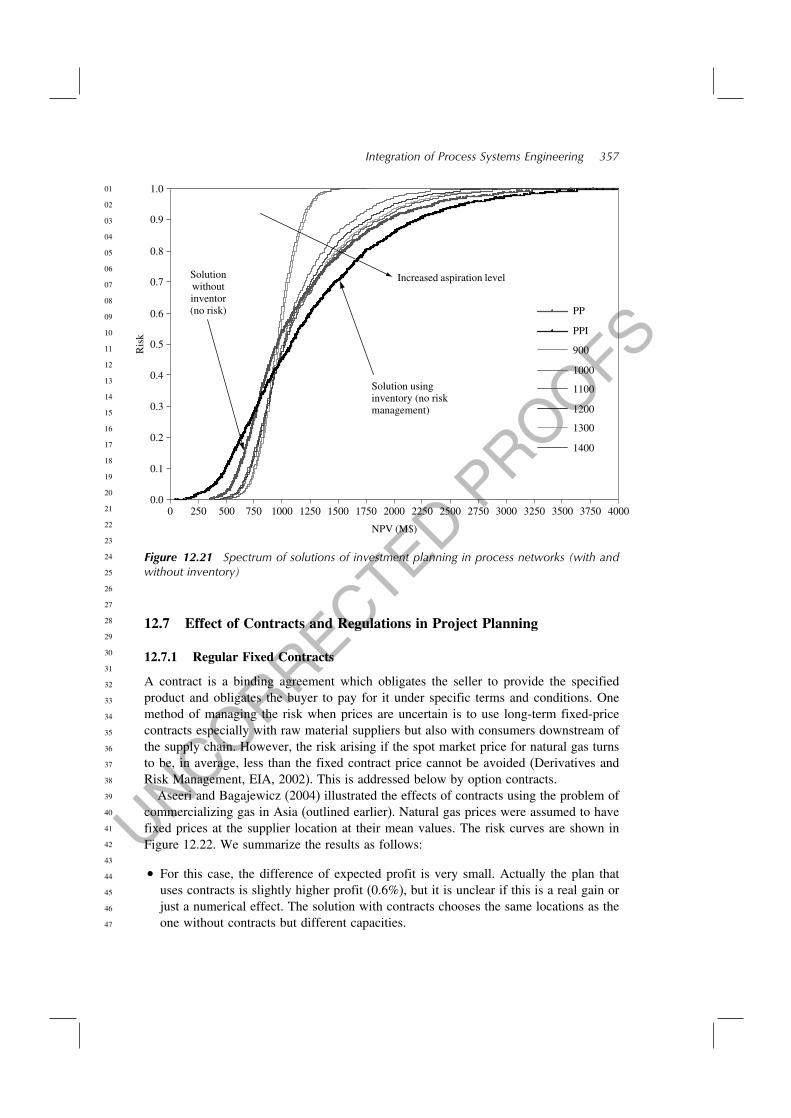
UNCORRECTED PROOFS

01

02

03

04

05

06

07

08

09

10

11

12

13

14

15

16

17

18

19

20

21

22

23

24

25

26

27

28

29

30

31

32

33

34

35

36

37

38

39

40

41

42

43

44

45

46

47


0.0

0.1

0.2

0.3

0.4

0.5

0.6

0.7

0.8

0.9

1.0

0 250 500 750 1000 1250 1500 1750 2000 2250 2500 2750 3000 3250 3500 3750 4000

NPV (M$)

Ris

k

PP

PPI

900

1000

1100

1200

1300

1400

Increased aspiration levelSolutionwithoutinventor(no risk)

Solution usinginventory (no riskmanagement)

Figure 12.21 Spectrum of solutions of investment planning in process networks (with andwithout inventory)

12.7 Effect of Contracts and Regulations in Project Planning

12.7.1 Regular Fixed Contracts

A contract is a binding agreement which obligates the seller to provide the specifiedproduct and obligates the buyer to pay for it under specific terms and conditions. Onemethod of managing the risk when prices are uncertain is to use long-term fixed-pricecontracts especially with raw material suppliers but also with consumers downstream ofthe supply chain. However, the risk arising if the spot market price for natural gas turnsto be, in average, less than the fixed contract price cannot be avoided (Derivatives andRisk Management, EIA, 2002). This is addressed below by option contracts.

Aseeri and Bagajewicz (2004) illustrated the effects of contracts using the problem ofcommercializing gas in Asia (outlined earlier). Natural gas prices were assumed to havefixed prices at the supplier location at their mean values. The risk curves are shown inFigure 12.22. We summarize the results as follows:

• For this case, the difference of expected profit is very small. Actually the plan thatuses contracts is slightly higher profit (0.6%), but it is unclear if this is a real gain orjust a numerical effect. The solution with contracts chooses the same locations as theone without contracts but different capacities.

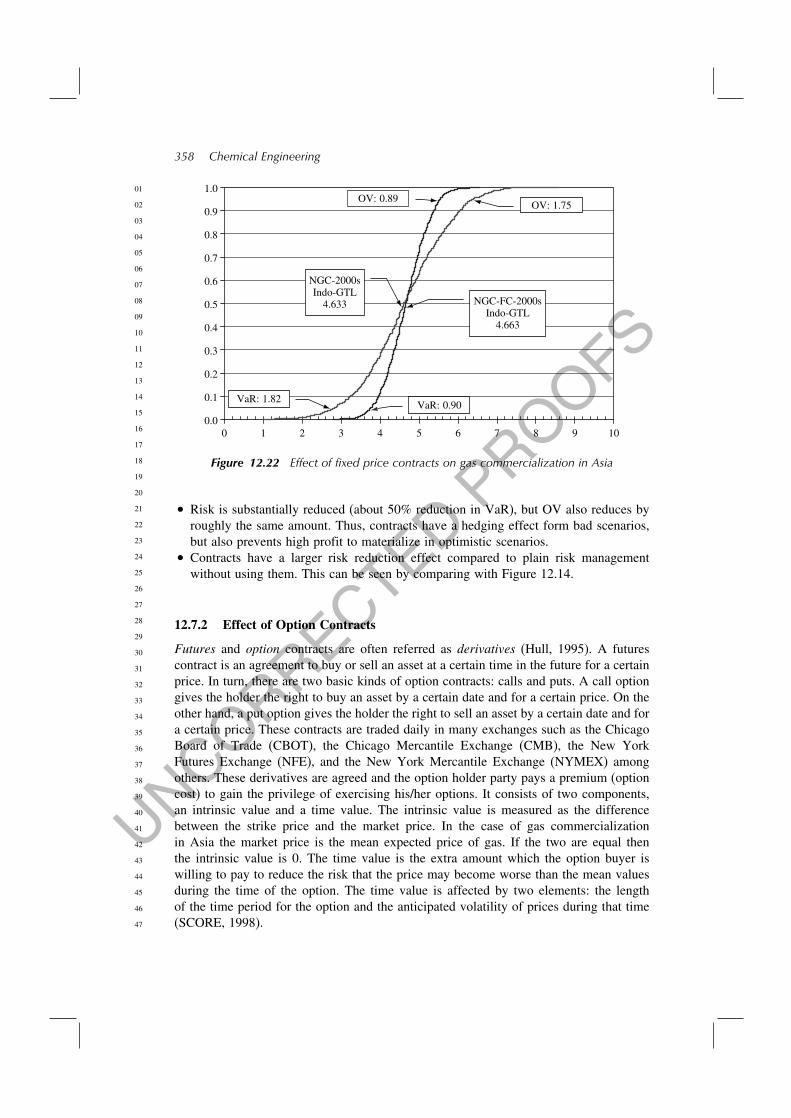
UNCORRECTED PROOFS

01

02

03

04

05

06

07

08

09

10

11

12

13

14

15

16

17

18

19

20

21

22

23

24

25

26

27

28

29

30

31

32

33

34

35

36

37

38

39

40

41

42

43

44

45

46

47


0.00

0.1

0.2

0.3

0.4

0.5

0.6

0.7

0.8

0.9

1.0

9 10

NGC-FC-2000sIndo-GTL

4.663

VaR: 1.82VaR: 0.90

OV: 1.75OV: 0.89

871 2 3 4 5 6

NGC-2000sIndo-GTL

4.633

Figure 12.22 Effect of fixed price contracts on gas commercialization in Asia

• Risk is substantially reduced (about 50% reduction in VaR), but OV also reduces byroughly the same amount. Thus, contracts have a hedging effect form bad scenarios,but also prevents high profit to materialize in optimistic scenarios.

• Contracts have a larger risk reduction effect compared to plain risk managementwithout using them. This can be seen by comparing with Figure 12.14.

12.7.2 Effect of Option Contracts

Futures and option contracts are often referred as derivatives (Hull, 1995). A futurescontract is an agreement to buy or sell an asset at a certain time in the future for a certainprice. In turn, there are two basic kinds of option contracts: calls and puts. A call optiongives the holder the right to buy an asset by a certain date and for a certain price. On theother hand, a put option gives the holder the right to sell an asset by a certain date and fora certain price. These contracts are traded daily in many exchanges such as the ChicagoBoard of Trade (CBOT), the Chicago Mercantile Exchange (CMB), the New YorkFutures Exchange (NFE), and the New York Mercantile Exchange (NYMEX) amongothers. These derivatives are agreed and the option holder party pays a premium (optioncost) to gain the privilege of exercising his/her options. It consists of two components,an intrinsic value and a time value. The intrinsic value is measured as the differencebetween the strike price and the market price. In the case of gas commercializationin Asia the market price is the mean expected price of gas. If the two are equal thenthe intrinsic value is 0. The time value is the extra amount which the option buyer iswilling to pay to reduce the risk that the price may become worse than the mean valuesduring the time of the option. The time value is affected by two elements: the lengthof the time period for the option and the anticipated volatility of prices during that time(SCORE, 1998).

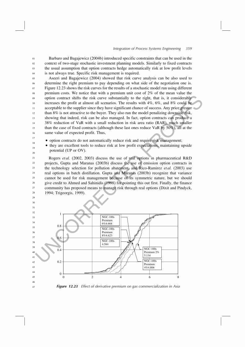
UNCORRECTED PROOFS

01

02

03

04

05

06

07

08

09

10

11

12

13

14

15

16

17

18

19

20

21

22

23

24

25

26

27

28

29

30

31

32

33

34

35

36

37

38

39

40

41

42

43

44

45

46

47


Barbaro and Bagajewicz (2004b) introduced specific constraints that can be used in thecontext of two-stage stochastic investment planning models. Similarly to fixed contractsthe usual assumption that option contracts hedge automatically risk at low profit levelsis not always true. Specific risk management is required.

Aseeri and Bagajewicz (2004) showed that risk curve analysis can be also used todetermine the right premium to pay depending on what side of the negotiation one is.Figure 12.23 shows the risk curves for the results of a stochastic model run using differentpremium costs. We notice that with a premium unit cost of 2% of the mean value theoption contract shifts the risk curve substantially to the right, that is, it considerablyincreases the profit at almost all scenarios. The results with 4%, 6%, and 8% could beacceptable to the supplier since they have significant chance of success. Any price greaterthan 8% is not attractive to the buyer. They also run the model penalizing downside risk,showing that indeed, risk can be also managed. In fact, option contracts can produce a38% reduction of VaR with a small reduction in risk area ratio (RAR), much smallerthan the case of fixed contracts (although these last ones reduce VaR by 50%), all at thesame value of expected profit. Thus,

• option contracts do not automatically reduce risk and require risk management;• they are excellent tools to reduce risk at low profit expectations, maintaining upside

potential (UP or OV).

Rogers et al. (2002, 2003) discuss the use of real options in pharmaceutical R&Dprojects, Gupta and Maranas (2003b) discuss the use of emission option contracts inthe technology selection for pollution abatement, and Rico-Ramirez et al. (2003) usereal options in batch distillation. Gupta and Maranas (2003b) recognize that variancecannot be used for risk management because of its symmetric nature, but we shouldgive credit to Ahmed and Sahinidis (1998) for pointing this out first. Finally, the financecommunity has proposed means to manage risk through real options (Dixit and Pindyck,1994; Trigeorgis, 1999).

0

0.2

0.4

0.6

0.8

1

0 2 4 6 8

NGC-100s4.584

NGC-100sPremium8%4.623



NGC-100sPremium 2%5.134

Figure 12.23 Effect of derivative premium on gas commercialization in Asia

UNCORRECTED PROOFS

01

02

03

04

05

06

07

08

09

10

11

12

13

14

15

16

17

18

19

20

21

22

23

24

25

26

27

28

29

30

31

32

33

34

35

36

37

38

39

40

41

42

43

44

45

46

47


12.7.3 Effect of Regulations

In a recent article Oh and Karimi (2004) explore the effect of regulations (bilateral andmultilateral international trade agreements, import tariffs, corporate taxes in differentcountries, etc.) on the capacity expansion problem. They point out that barring the workof Papageorgiou et al. (2001), who explore the effect of corporate taxes in the opti-mization of a supply chain for a pharmaceutical industry, very little attempt has beenmade to incorporate other regulatory issues in the capacity expansion problem. However,they point out to other attempts in location-allocation problems and in production-distribution problems (Cohen et al., 1989; Arntzen et al., 1995; Goetschalckx et al.,2002), which include tariffs, duty drawbacks, local content rules, etc. for a multinationalcorporation.

12.8 Integration of Operations Planning and Budgeting

Cash flow needs to be managed at the first stage, not at the second stage. This iscontained in the pioneering work of Badell and Puigjaner (1998), Badell and Puigjaner(2001a,b), Romero et al. (2003a,b), and Badell et al. (2004). In these articles, the groupof Professor Puigjaner establishes the links between procuring, financial management,and manufacturing, that is, proposes the use of models that break the walls existingbetween these three entities. Basically, deterministic cash flow is considered at the sametime as scheduling of operations, batch plants in this case. The articles provide alsosome background on the literature of cash management models and the need to useand integrate them. More specifically, Romero et al. (2003a) propose the merging ofscheduling and planning with cash management models (Charnes et al., 1959; Robicheket al., 1965; Orgler, 1970; Srinivasan, 1986). Their model shows that the profit increasesby considering these activities together because procuring does not buy expensive rawmaterials too early in the process. The integrated approach, instead, proposes to rearrangethe schedule to accumulate some cash to buy these expensive raw materials. The root ofthe difference is not only better cash management, but also a departure from Miller andOrr’s (1966) model (Figure 12.24), where it is recommended to borrow or buy securities,only when a lower or upper bound is reached. A flat profile, like the one in Figure 12.25,

A′

B′

Upper bound

Time

Lower bound

ANet cash

flowbalance

Ideallevel

B′

Figure 12.24 Miller and Orr’s cash management model

UNCORRECTED PROOFS

01

02

03

04

05

06

07

08

09

10

11

12

13

14

15

16

17

18

19

20

21

22

23

24

25

26

27

28

29

30

31

32

33

34

35

36

37

38

39

40

41

42

43

44

45

46

47


Time

Lower bound

Net cash flow

balance

Ideallevel

Figure 12.25 Ideal cash flow model

is desirable, and achievable only with the integrated model. In this flat profile, one onlysees spikes due, for example, to the short span between the inflow of cash and the buyingof securities. As one can see, no downward spikes are observed because the outflow ofmoney can be planned.

Romero et al. (2003a) also present preliminary work where the above ideas are alsoextended to consider uncertainty and financial risk. Some sort of budgeting, although notfull cash management, was considered by Van den Heever et al. (2000) where royaltypayments are taken into account in the offshore drilling problem. Although royaltieswere not included, full cash management with uncertainty was considered by Aseeri et al.(2004) for the same offshore oil drilling problem, results of which have been outlinedabove. Van den Heever and Grossmann (2000) proposed an aggregation/disaggregationmethod to solve the problem. The same group of researchers added tax and royaltycalculations to the problem, which increased its numerical complexity (Van den Heeveret al., 2000) and studied the use of big-M constraints as well as disjunctive program-ming. Finally, Van den Heever et al. (2001) proposed a Lagrangean decompositionprocedure.

12.9 Integration of Operations Planning and Pricing

Guillén et al. (2003a) suggested that pricing policies considered in an integrated mannerwith scheduling decisions (integration of manufacturing and marketing) increase profit.They discuss the existing models for pricing and point out that the supply curve, which isdependent on manufacturing costs, can be altered. In other words, altering the productionschedule should and indeed does have an effect on the fixed costs per unit used in exist-ing classical pricing models (Dorward, 1987; Mas-Collel et al., 1995). They assumed aniterative model in which product prices are first fixed to obtain a schedule, which inturn can be used again in an iterative manner to obtain new product costs which enablethe calculation of new process. They showed that this model not always converges.Moreover, an alternative model in which process and production schedules are obtainedsimultaneously is proposed. The integrated model, they show, produces different sched-ules and prices and allows larger profits. Indeed, for a case of three products, the iterative

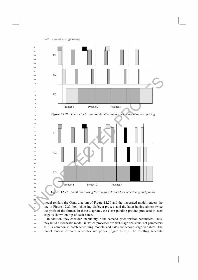
UNCORRECTED PROOFS

01

02

03

04

05

06

07

08

09

10

11

12

13

14

15

16

17

18

19

20

21

22

23

24

25

26

27

28

29

30

31

32

33

34

35

36

37

38

39

40

41

42

43

44

45

46

47


Product 1

U1

U2

U3

Product 2 Product 3

Figure 12.26 Gantt chart using the iterative method for scheduling and pricing

Product 1

U1

U2

U3

Product 2 Product 3

Figure 12.27 Gantt chart using the integrated model for scheduling and pricing

model renders the Gantt diagram of Figure 12.26 and the integrated model renders theone in Figure 12.27, both choosing different process and the latter having almost twicethe profit of the former. In these diagrams, the corresponding product produced in eachstage is shown on top of each batch.

In addition, they consider uncertainty in the demand–price relation parameters. Thus,they build a stochastic model, in which processes are first-stage decisions, not parametersas it is common in batch scheduling models, and sales are second-stage variables. Themodel renders different schedules and prices (Figure 12.28). The resulting schedule

UNCORRECTED PROOFS

01

02

03

04

05

06

07

08

09

10

11

12

13

14

15

16

17

18

19

20

21

22

23

24

25

26

27

28

29

30

31

32

33

34

35

36

37

38

39

40

41

42

43

44

45

46

47


Product 1

U1

U2

U3

Product 2 Product 3

Figure 12.28 Gantt chart for the stochastic case for scheduling and pricing

implies a mixed product campaign and not a single product campaign as occurred in thedeterministic case. This schedule seems to be more robust.

In order to show the capability of the proposed formulation of risk management, theproblem is modified so as to reduce the risk associated at low targets. The Gantt chartcorresponding to one solution with lower risk and consequently lower expected profit isshown in Figure 12.29. The risk curves of both the stochastic solution (SP) and the onewith lower risk are shown in Figure 12.30. The risk at low expectations (profits under atarget of $6500) was reduced to 0.

Product 1

U1

U2

U3

Product 2 Product 3

Figure 12.29 Gantt chart for the risk managing solution for scheduling and pricing

UNCORRECTED PROOFS

01

02

03

04

05

06

07

08

09

10

11

12

13

14

15

16

17

18

19

20

21

22

23

24

25

26

27

28

29

30

31

32

33

34

35

36

37

38

39

40

41

42

43

44

45

46

47


0

10

20

30

40

50

60

70

80

90

100

5200 7200 9200 11 200 13 200

Profit

Ris

k (%

)

SP

Ω = 6500

Figure 12.30 Risk curves for scheduling and pricing

12.10 Consumer Satisfaction

Consumer satisfaction was considered in conjunction with supply chain management byTsiakis et al. (2001). They measure it using the quotient between sales and demand.Guillén et al. (2003b) study a similar problem, a supply chain with warehouses, markets,and distribution centers. Instead of constraining the customer satisfaction, they assume amultiobjective model and construct a Pareto surface. They also solve a stochastic modelwhere demands are uncertain, the opening of plants/warehouses is first-stage variablesand the sales are second-stage variables. The two resulting Pareto curves are different(Figures 12.31 and 12.32) revealing the need for stochastic models. Moreover, they definecustomer satisfaction risk and discuss the interrelation between three different objectives:NPV, customer satisfaction, and financial risk. Finally, they define compounded risk andevaluate it through composite curves (Figure 12.33).

3.00

3.10

3.20

3.30

3.40

3.50

3.60

60 70 80 90 100Customer satisfaction (%)

NPV

(m

illio

ns o

f eu

ros)

Figure 12.31 Deterministic Pareto curve profit–customer satisfaction

UNCORRECTED PROOFS

01

02

03

04

05

06

07

08

09

10

11

12

13

14

15

16

17

18

19

20

21

22

23

24

25

26

27

28

29

30

31

32

33

34

35

36

37

38

39

40

41

42

43

44

45

46

47


3.00

3.10

3.20

3.30

3.40

3.50

3.60

60 70 80 90 100

Expected customer satisfaction (%)

Expec

ted N

PV

(m

illi

ons

of

euro

s)

Figure 12.32 Stochastic Pareto curve profit–customer satisfaction

1.0

0.8

0.6

0.4

0.2

0

Ris

k

90

80

70

60 2.53.0

3.54.0

Omega = 75E(CSAT) > 0

Customersatisfaction (%) NPV (€)

Figure 12.33 Composite financial and consumer satisfaction risk curves

12.11 Product Engineering and Process Engineering

In recent years, several authors advocated that process system engineers should payincreased attention to a new paradigm, that of product design, one eventually (andapparently) opposed to process design (Westerberg and Subramanian, 2000; Cusslerand Moggridge, 2001). The suggestion, although implicit, is that process engineeringis a mature field, while product design is a relatively virgin field, at least virgin fromthe use of tools and methods of the PSE community. One good example of effortsfollowing the suggested path is the article by Wibowo and Ng (2001), who analyze theissues associated with the fabrication of creams and pastes. We already mentioned in thepreceding text several articles dealing with drug development, which are in fact product

UNCORRECTED PROOFS

01

02

03

04

05

06

07

08

09

10

11

12

13

14

15

16

17

18

19

20

21

22

23

24

25

26

27

28

29

30

31

32

33

34

35

36

37

38

39

40

41

42

43

44

45

46

47


Table 12.4 Process design versus product design(taken from Cussler, 2003)

Process design Product design

1. Batch vs. continuous 1. Customer need2. Input/Output 2. Idea generation3. Recycles 3. Selection4. Separation/Heat 4. Manufacture

design. Following the same trend, Cussler (2003) illustrates some of the differencesbetween the two paradigms (Table 12.4). To do the comparison he uses the so-calledconceptual design paradigm (Douglas, 1988), which is very similar to the onion model(Smith and Linnhoff, 1988; Smith, 1995), and is widely used. This is the order thatmany books on process and product design follow (Seider et al., 2004). There are ofcourse other approaches to process design, like the reducible superstructure approach(best represented by the book of Biegler et al., 1997). The table, nonetheless, has a coupleof interesting features.

1) Makes product design the center.2) Suggests ad hoc idea generation and selection steps that presumably vary from product

to product, for which a systematic search is not available or has to be constructedcase by case (Cussler and Moggridge, 2001). We have seen examples on searchesdriven by functionalities (refrigerants, drugs, etc.) like those performed by Camardaand Maranas (1999) and Sahinidis and Tawarlamani (2000) and also described byAchenie et al. (2002).

3) In fact, some who advocate product design (Cussler and Moggridge, 2001) only callit chemical product design, which rules out mechanical and electronic and electrome-chanical devices, etc. In fact, it is only a matter of time until this expands to allproducts. Evans (2003), for example, has recently emphasized the upcoming inte-gration between the process industries as providers of commodities and the discreteindustries the providers of package goods, devices, appliances, automobiles, etc.

4) Its title suggests that these are somehow opposite and to an extent excluding activities.

Recently, Stephanopoulos (2003) reemphasized the idea of product design and sug-gested that manufacturing is indeed migrating from process (commodity)-centric toproduct-centric, all this judged by the performance of the companies in the stock market.He suggests that a company should maximize value-addition through the supply chain andthat while the process-centered industry focuses on commodities, the product-centeredindustry focuses on identification of customer needs as a driving force. He asks whether‘Process Systems Engineering is prepared to engineer (design and manufacture) products,or someone else should do it?’ One must wonder whether he refers to the role of chemicalengineers in all end-user products, not only chemical products.

In parallel to this push for extending the borders of chemical process systems engineer-ing to areas that have been traditional to industrial engineers, a new concept of supplychemical chain was recently discussed in detail by Grossmann and Westerberg (2000),and in the United States National Academies report by Breslow and Tirrell (2003). Thechemical supply chain extends from the molecule level to the whole enterprise. Breslowand Tirrell (2003) suggest that

UNCORRECTED PROOFS

01

02

03

04

05

06

07

08

09

10

11

12

13

14

15

16

17

18

19

20

21

22

23

24

25

26

27

28

29

30

31

32

33

34

35

36

37

38

39

40

41

42

43

44

45

46

47


Another important aspect in the modeling and optimization of the chemical supply chainis the description of the dynamics of the information and material flow through the chain.This will require a better understanding of the integration of R&D, process design, processoperation, and business logistics. The challenge will be to develop quantitative modelsthat can be used to better coordinate and optimize the chemical enterprise. Progress willbe facilitated by new advances in information technology, particularly through advancesin the Internet and by new methods and mathematical concepts. Advances in computertechnology will play a central role. Fulfilling the goal of effectively integrating the variousfunctions (R&D, design, production, logistics) in the chemical supply chain will help tobetter meet customer demands, and effectively adapt in the new world of e-commerce.Concepts related to planning, scheduling, and control that have not been widely adoptedby chemical engineers should play a prominent role in the modeling part of this problem.Concepts and tools of computer science and operations research will play an even greaterrole in terms of impacting the implementation of solutions for this problem. (The bold andunderline was added)

The report cites the need of ‘integration of several parts of the chemical supplychain’, which ‘will give rise to a number of challenges, such as multi-scale modeling formolecular dynamics, integration of planning, scheduling and control (including Internetbased), and integration of measurements, control, and information systems’, but fallsshort of discussing the full integration with economics management and business.

It is here suggested that:

1) Process engineering, which is mistakenly associated with the production of commodi-ties, is an integral part of product design. Product design cannot exist without processdesign. So there is no antagonism of any sort.

2) When the chemical supply chain is considered in the context of process design, onerealizes that the chemical supply chain contains many of the elements of productdesign. Indeed, it deals with the chemistry, the selection, the manufacturing, and thesupply chain of entire enterprises, single- or multi-company, as in the alliances thatStephanopoulos (2003) suggested, that deliver the product to the customer.

Thus, product design, the newly proposed paradigm, can be constructed by putting mar-keting (idea generation and other tools) in front of the chemical supply chain, recognizingthat process systems engineering is an essential tool used in the chemical supply chainand putting the customer and the market at both ends of the supply chain, upfront as anobject of study for its needs and potential responses, and at the other end as the entity thatshapes the demand and provides the feedback (Figure 12.34). Or perhaps, the chemicalsupply chain box needs to be broken apart into smaller pieces, each of one interactingwith the rest in different forms.

Some elements addressing how one might address all these decision-making processesare described by Pekny (2002) who explores the role of different algorithm architecturesin large-scale engineering problems.

We notice that in the figure the interactions are in both directions, suggesting that thereis no sequential approach, as Cussler would suggest, but rather the notion that, since allactivities influence each other, we ought to consider them simultaneously. We have alsoadded some dotted line boxes to indicate that integrated models already exist betweenthe different segments. Noticeably, the upfront identification of customer needs is notyet integrated with the rest of the activities. There is therefore a need for modeling inthis area.

UNCORRECTED PROOFS

01

02

03

04

05

06

07

08

09

10

11

12

13

14

15

16

17

18

19

20

21

22

23

24

25

26

27

28

29

30

31

32

33

34

35

36

37

38

39

40

41

42

43

44

45

46

47


Customer– Needs– Potential reactions

Chemical supply chain

– Modeled from the molecule to the multi-company enterprise– Using process engineering tools– Integrating business tools

Customer– Demands– Satisfaction– Feedback, etc.

Management and finances

– Working capital models– Risk analysis– Budgeting models, etc.

Advertising Humanrelations (labor)

SociologyPsychologyPublic policyAdvertising

Figure 12.34 Product development and delivery supply chain

12.12 Retrofit

While most engineering assumes grass-roots activities, the issue of revamping the existinginfrastructure of a company is sometimes even more challenging and it certainly involvesthe integration with finances. We leave specifically for some other discussion the retrofitactivity of the existing industry.

12.13 The Environment

A lot was discussed in late years about sustainability and the global life cycle assessmentof processes and products (Nebel and Wright, 2002). While some authors have started toincorporate this as constraints in process design, others have opted to leave sustainability(or some equivalent measure) as an alternative objective to be considered together withprofitability and perhaps financial risk in Pareto surfaces (Cheng et al., 2003). Grossmann(2003) discusses some of what he calls ‘timid’ efforts by the process systems engineeringcommunity in assessing sustainability (Marquardt et al., 2000) and there are already workon industrial ecology performed by chemical engineers (Bakshi, 2000; Bakshi and Fiskel,2003). Batterham (2003) provides an insightful analysis of sustainability emphasizing thefact that sustainability isno longeraconstraint thatcomesfromregulationsand it isbecominga genuine objective of corporations in such a way that ‘both companies and society canbenefit’. Time will tell how genuine these efforts are. It is claimed here that sustainabilityis both a constraint and an alternative objective, leaving the analysis for future work.

12.14 Conclusions

This is not a review of the large number of developments concerning the integrationof business tools with process and product engineering. Rather, some tools that helpthe integration, which has been recently proposed and used, are pointed out. The article

UNCORRECTED PROOFS

01

02

03

04

05

06

07

08

09

10

11

12

13

14

15

16

17

18

19

20

21

22

23

24

25

26

27

28

29

30

31

32

33

34

35

36

37

38

39

40

41

42

43

44

45

46

47


focuses on financial risk and proposes that the proper paradigm is through handling ofrisk curves, especially if they are immersed in a two- (or multi-) stage stochastic model.It also proposed to stress out the connections to shareholder value.

Full integration of several disciplines – management, finances, industrial engineering,and chemical engineering, among others – is slowly taking place. The result is thisbeginning to end modeling of the product research/development and delivery supplychain. In turn, more interactions with other disciplines (public policy, psychology, etc.)will come. At some point, with powerful computers and adequate modeling, one candream of a full integration of the whole process in one single model. Then, one canstart to ask if with so much access to information and with so many tools to respondoptimally, we will reach a state where competition will cease to have a meaning.

Acknowledgements

After we presented our first article on risk management in the 1999 AIChE Meeting (Roderaand Bagajewicz, 2000), we got busy developing the theory first (Barbaro and Bagajewicz,2003, 2004a,b), and worked on applications of our theory to several problems. Some ofthese experiences are summarized in this chapter. I thank deeply my students who wereinstrumental in helping me articulate the vision. A fruitful sabbatical stay with the groupof Dr Lluis Puigjaner at the Polytechnic of Catalunya (UPC) taught me invaluable lessonsthrough many passionately argued ideas and discussions with students and professors.

My thanks also go to the following persons who read my original manuscriptand were instrumental in improving it: Arthur Westerberg and Ignacio Grossmann(Carnegie Mellon University), Anshuman Gupta and Costas Maranas (Pennsylvania StateUniversity), Frank Zhu and Gavin Towler (UOP), Larry Evans (Aspentech), JeffreySiirola (Eastman), and Jesus Salas (University of Oklahoma).

Finally, I thank the organizers of this symposium for the financial support and theopportunity to think out loud.

References

[1] Achenie L.E.K., Gani R. and Venkatasubramanian V. 2002 (Eds.). Computer Aided MolecularDesign: Theory and Practice. Elsevier Publishers.

[2] Ahmed S. and Sahinidis N.V. 1998. Robust process planning under uncertainty, Ind. Eng.Chem. Res., 37(5), 1883–1892.

[3] Ahmed S. and Sahinidis N.V. 2000a. Analytical investigations of the process planning problem,Comput. Chem. Eng., 23(11–12), 1605–1621.

[4] Ahmed S. and Sahinidis N.V. 2000b. Selection, acquisition and allocation of manufacturingtechnology in a multi-product environment, Manage. Sci. (submitted).

[5] Applequist G., Pekny J.F. and Reklaitis G.V. 2000. Risk and uncertainty in managing chemicalmanufacturing supply chains, Comput. Chem. Eng., 24(9/10), 2211.

[6] Arntzen B., Brown G., Harrison T. and Trafton L. 1995. Global supply chain management atdigital equipment corporation, Interfaces, 25, 69.

[7] Aseeri A., Gorman P. and Bagajewicz M. 2004. Financial risk management in offshore oilinfrastructure planning and scheduling, Ind. Eng. Chem. Res. 43(12), 3063–3072 (special issuehonoring George Gavalas).

UNCORRECTED PROOFS

01

02

03

04

05

06

07

08

09

10

11

12

13

14

15

16

17

18

19

20

21

22

23

24

25

26

27

28

29

30

31

32

33

34

35

36

37

38

39

40

41

42

43

44

45

46

47


[8] Aseeri A. and Bagajewicz M. 2004. New measures and procedures to manage financial riskwith applications to the planning of gas commercialization in Asia, Comput. Chem. Eng.,28(12), 2791–2821.

[9] Badell M. and Puigjaner L.A. 1998. New conceptual approach for enterprise resource man-agement systems. In, FOCAPO AIChE Symposium Series, New York, Pekny J.F. and BlauG.E. (Eds.), Vol. 94, No. 320, p. 217.

[10] Badell M. and Puigjaner L. 2001a. Discover a powerful tool for scheduling in ERM systems,Hydrocarbon Process., 80(3), 160.

[11] Badell M. and Puigjaner L. 2001b. Advanced enterprise resource management systems,Comput. Chem. Eng., 25, 517.

[12] Badell M., Romero J., Huertas R. and Puigjaner L. 2004. Planning, scheduling and budgetingvalue-added chains, Comput. Chem. Eng., 28, 45–61.

[13] Bagajewicz M. 2000. A review of recent design procedures for water networks in refineriesand process plants, Comput. Chem. Eng., 24(9), 2093–2115.

[14] Bagajewicz M. and Barbaro A.F. 2003. Financial risk management in the planning of energyAQ: 1

recovery in the total site, Ind. Eng. Chem. Res., 42(21), 5239–5248.[15] Bakshi B.R. 2000. A thermodynamic framework for ecologically conscious process systems

engineering, Comput. Chem. Eng., 24, 1767–1773.[16] Bakshi B.R. and Fiskel J. 2003. The quest for sustainability: challenges for process systems

engineering, AIChE J., 49(6), 1350–1358.[17] Barbaro A. and Bagajewicz M. 2003. Financial risk management in planning under uncer-

tainty. FOCAPO 2003 (Foundations of Computer Aided Process Operations), Coral Springs,FL, USA, January 2003.

[18] Barbaro A.F. and Bagajewicz M. 2004a. Managing financial risk in planning under uncer-tainty, AIChE J., 50(5), 963–989.

[19] Barbaro A.F. and Bagajewicz M. 2004b. Use of inventory and option contracts to hedgefinancial risk in planning under uncertainty, AIChE J., 50(5), 990–998.

[20] Batterham R.J. 2003. Ten years of sustainability: where do we go from here?, Chem. Eng.Sci., 58, 2167–2179.

[21] Bellman R.E. 1957. Dynamic Programming. Princeton University Press.[22] Berger J.O. 1980. Statistical Decision Theory. Springer-Verlag, New York.[23] Biegler L., Grossmann I.E. and Westerberg A.W. 1997. Systematic Methods of Chemical

Process Design. Prentice Hall, New Jersey.[24] Birge J.R. and Louveaux F. 1997. Introduction to Stochastic Programming. Springer,

New York.[25] Blau G., Mehta B., Bose S., Pekny J., Sinclair G., Keunker K. and Bunch P. 2000. Risk

management in the development of new products in highly regulated industries, Comput.Chem. Eng., 24, 659–664.

[26] Blau G.E. and Sinclair G. 2001. Dealing with uncertainty in new product development, CEP,97(6).

[27] Bok J., Lee H. and Park S. 1998. Robust investment model for long range capacity expansionof chemical processing networks under uncertain demand forecast scenarios, Comput. Chem.Eng., 22, 1037–1050.

[28] Bok J., Grossmann I.E. and Park S. 2000. Supply chain optimization in continuous flexibleprocess networks, Ind. Eng. Chem. Res., 39, 1279–1290.

[29] Bonfill A., Bagajewicz M., Espuña A. and Puigjaner L. 2004. Risk management in schedulingof batch plants under uncertain market demand, Ind. Eng. Chem. Res., 43(9), 2150–2159.

[30] Bose S. and Pekny J.F. 2000. A model predictive framework for planning and schedulingproblems: a case study of consumer goods supply chain, Comput. Chem. Eng., 24(2–7),329–335.

UNCORRECTED PROOFS

01

02

03

04

05

06

07

08

09

10

11

12

13

14

15

16

17

18

19

20

21

22

23

24

25

26

27

28

29

30

31

32

33

34

35

36

37

38

39

40

41

42

43

44

45

46

47


[31] Breslow R. and Tirrell M.V. (Co-Chairs). 2003. Beyond the molecular frontier. challengesfor chemistry and chemical engineering. Committee on Challenges for the Chemical Sciencesin the 21st Century. The United States National Academies Press.

[32] Bunch P.R. and Iles C.M. 1998. Integration of planning and scheduling systems with manu-facturing business processes, Annual AIChE Meeting.

[33] Byrd L.R. and Chung F.T.-H. 1998. Risk analysis and decision-making software packageuser’s manual. Prepared for the US DOE, National Petroleum Technology Office.

[34] Camarda K.V. and Maranas C.D. 1999. Optimization in polymer design using connectivityindices, Ind. Eng. Chem. Res., 38, 1884–1892.

[35] Charnes A. and Cooper W.W. 1959. Chance-constrained programming, Manag. Sci., 6, 73.[36] Charnes A., Cooper W.W. and Miller M.H. 1959. Application of linear programming to

financial budgeting and the costing of funds. In, The Management of Corporate Capital,Solomon E. (Ed.). Free Press of Glencoe, Illinois.

[37] Cheng, L., Subrahmanian E. and Westerberg A.W. 2003. Design and planning under uncer-tainty: issues on problem formulation and solution, Comput. Chem. Eng., 27(6), 781–801.

[38] Cheng, L., Subrahmanian E. and Westerberg A.W. 2004. Multi-objective decisions on capac-ity planning and production-inventory control under uncertainty, Ind. Eng. Chem. Res., 43,2192–2208.

[39] Cheung R.K.M. and Powel W.B. 2000. Shape – a stochastic hybrid approximation procedurefor two-stage stochastic programs, Oper. Res., 48(1), 73–79.

[40] Cohen M.A., Fisher M. and Jaikumar R. 1989. International manufacturing and distributionnetworks: a normative model framework. In, Managing International Manufacturing, FerdowsK. (Ed.). Amsterdam, North Holland, p. 67.

[41] Cussler E.L. 2003. Chemical Product Design and Engineering (Plenary Talk). AIChE AnnualConference, San Francisco. Paper 430a, November 2003.

[42] Cussler E.L. and Moggridge G.D. 2001. Chemical Product Design, 1st edition. CambridgeUniversity Press.

[43] Dahl H., Meeraus A. and Zenios S. 1993. Some financial optimization models: I Riskmanagement. In, Financial Optimization, Zenios S.A. (Eds.). Proceedings of a Conferenceheld at the Wharton School, University of Pennsylvania, Philadelphia, USA.

[44] Danthine J.P. and Donaldson J.B. 2002. Intermediate Financial Theory. Prentice Hall,New Jersey.

[45] De Reyck B., Degraeve Z. and Vandenborre R. 2001. Project Options Valuation with NetPresent Value and Decision Tree Analysis. Working Paper, London Business School. Pre-sented at 2001 INFORMS. INFORMS Conference, Miami Beach, November.

[46] Debreu G. 1959. Theory of Value. An Axiomatic Analysis of Economic Equilibrium.John Wiley, New York.

[47] Denardo E.V. 1982. Dynamic Programming: Models and Applications. Prentice Hall,New Jersey.

[48] Dixit A.K. and Pindyck R.S. 1994. Investment under Uncertainty. Princeton University Press,Princeton, NJ.

[49] Dorward N. 1987. The Price Decision: Economic Theory and Business Practice. Harper &Row, London.

[50] Douglas J.M. 1988. Conceptual Design of Chemical Processes. McGraw Hill, New York.[51] Dupacova J. and Römisch W. 1998. Quantitative stability for scenario-based stochastic

programs, Prague Stochastics 98, S. 119–124, JCMF, Praha.[52] EIA. 2002. Derivatives and Risk Management in the Petroleum, Natural Gas, and

Electricity Industries. Energy Information Administration, October 2002. Available athttp://www.eia.doe.gov.

[53] Eppen G.D, Martin R.K. and Schrage L. 1989. A scenario approach to capacity planning.Oper. Res., 37, 517–527.

UNCORRECTED PROOFS

01

02

03

04

05

06

07

08

09

10

11

12

13

14

15

16

17

18

19

20

21

22

23

24

25

26

27

28

29

30

31

32

33

34

35

36

37

38

39

40

41

42

43

44

45

46

47


[54] Espuña A., Rodrigues M.T., Gimeno L. and Puigjaner L. 2003. A holistic framework forsupply chain management. Proceedings of ESCAPE 13. Lappeenranta, Finland, 1–4 June.

[55] Evans L. 2003. Achieving Operational Excellence with Information Technology. AICHESpring Meeting, New Orleans, March.

[56] Finnerty J.E. 1993. Planning Cash Flow. AMACON (American Management Association),New York.

[57] Gaur V. and Seshadri S. 2004. Hedging Inventory Risk through Market Instruments. WorkingPaper at the Stern School of Business, New York University.

[58] Gjerdrum J., Shah N. and Papageorgiou L.G. 2001. Transfer prices for multienterprise supplychain optimization, Ind. Eng. Chem. Res., 40, 1650–1660.

[59] Goetschalckx M., Vidal C.J. and Dogan K. 2002. Modeling and design of global logisticssystems: a review of integrated strategic and tactical models and design algorithms, Eur. J.Oper. Res., 143, 1.

[60] Gregory G. 1988. Decision Analysis. Plenum Press, New York.[61] Grossmann I.E. 2003. Challenges in the new millennium: product discovery and design, enter-

prise and supply chain optimization, global life cycle assessment. PSE 2003. 8th InternationalSymposium on Process Systems Engineering, China.

[62] Grossmann I.E. and Westerberg A.W. 2000. Research challenges in process systems engi-neering. AIChE J., 46, 1700–1703.

[63] Guillén G., Bagajewicz M., Sequeira S.E., Tona R., Espuña A. and Puigjaner L. 2003a.Integrating pricing policies and financial risk management into scheduling of batch plants.PSE 2003. 8th International Symposium on Process Systems Engineering, China, June 2003.

[64] Guillén G., Mele F., Bagajewicz M., Espuña A. and Puigjaner L. 2003b. Management offinancial and consumer satisfaction risks in supply chain design. Proceedings of ESCAPE13. Lappeenranta, Finland, 1–4 June 2003.

[65] Guldimann T. 2000. The story of risk metrics, Risk, 13(1), 56–58.[66] Gupta A. and Maranas C.D. 2000. A two-stage modeling and solution framework for multisite

midterm planning under demand uncertainty, Ind. Eng. Chem. Res., 39, 3799–3813.[67] Gupta A. and Maranas C. 2003a. Managing demand uncertainty in supply chain planning,

Comput. Chem. Eng., 27, 1219–1227.[68] Gupta A. and Maranas C. 2003b. Market-based pollution abatement strategies: risk manage-

ment using emission option contracts, Ind. Eng. Chem. Res., 42, 802–810.[69] Gupta A. and Maranas C. 2004. Real-options-based planning strategies under uncertainty,

Ind. Eng. Chem. Res., 43(14), 3870–3878.[70] Gupta A., Maranas C.D. and McDonald C.M. 2000. Midterm supply chain planning under

demand uncertainty: customer demand satisfaction and inventory management, Comput.Chem. Eng., 24, 2613–2621.

[71] Hax A.C. and Majluf N.S. 1984. Strategic Management: An Integrated Perspective. PrenticeHall, New Jersey.

[72] Higle J.L. and Sen S. 1996. Stochastic Decomposition. A Statistical Method for Large ScaleStochastic Linear Programming. Kluwer Academic Publishers, Norwell, MA.

[73] Hull J. 1995. Introduction to Futures and Options Markets. Prentice Hall, EnglewoodCliffs, NJ.

[74] Ierapetritou M.G. and Pistikopoulos E.N. 1994. Simultaneous incorporation of flexibilityand economic risk in operational planning under uncertainty, Comput. Chem. Eng., 18(3),163–189.

[75] Ierapetritou M.G., Pistikopoulos E.N. and Floudas C.A. 1994. Operational planning underuncertainty, Comput. Chem. Eng., 18(Suppl.), S553–S557.

[76] Infanger G. 1994. Planning under Uncertainty: Solving Large-Scale Stochastic Linear Pro-grams. Boyd and Fraser, Danvers, MA.

[77] Iyer R.R. and Grossmann I.E. 1998a. A bilevel decomposition algorithm for long-rangeplanning of process networks, Ind. Eng. Chem. Res., 37, 474–481.

UNCORRECTED PROOFS

01

02

03

04

05

06

07

08

09

10

11

12

13

14

15

16

17

18

19

20

21

22

23

24

25

26

27

28

29

30

31

32

33

34

35

36

37

38

39

40

41

42

43

44

45

46

47


[78] Iyer R.R. and Grossmann I.E. 1998b. Synthesis of operational planning of utility systemsfor multiperiod operation, Comput. Chem. Eng., 22, 979–993.

[79] Iyer R.R., Grossmann I.E., Vasantharajan S. and Cullick A.S. 1998. Optimal planning andscheduling of offshore oil field infrastructure investment and operations, Ind. Eng. Chem.Res., 37, 1380–1397.

[80] Jackson J.R. and Grossmann I.E. 2003. Temporal decomposition scheme for nonlinear multi-site production planning and distribution models, Ind. Eng. Chem. Res., 42, 3045–3055.

[81] Jia J. and Dyer J.S. 1995. Risk-Value Theory. Working Paper, Graduate School of Business,University of Texas at Austin. Presented at INFORMS Conference, Los Angeles.

[82] Jia Z., Ierapetritou M. and Kelly J.D. 2003. Refinery short-term scheduling using continuoustime formulation: crude oil operations, Ind. Eng. Chem. Res., 42, 3085–3097.

[83] Joly M. and Pinto J.M. 2003. Mixed-integer programming techniques for the scheduling offuel oil and asphalt production, Trans. IChemE, 81(Part A).

[84] Jorion P. 2000. Value at Risk. The New Benchmark for Managing Financial Risk, 2ndedition. McGraw Hill, New York.

[85] Julka N., Srinivasan R. and Karimi I. 2002a. Agent-based supply chain management-1:framework, Comput. Chem. Eng., 26, 1755–1769.

[86] Julka N., Karimi I. and Srinivasan R. 2002b. Agent-based supply chain management-2:a refinery application, Comput. Chem. Eng., 26, 1771–1781.

[87] Kall P. and Wallace S.W. 1994. Stochastic Programming. John Wiley & Sons, Chichester.[88] Keown A.J., Martin J.D., Petty J.W. and Scott D.F. 2002. Financial Management: Principles

and Applications, 9th edition. Prentice Hall, New Jersey.[89] Koppol A. and Bagajewicz M. 2003. Financial risk management in the design of water

utilization systems in process plants, Ind. Eng. Chem. Res., 42(21), 5249–5255.[90] Koppol A., Bagajewicz M., Dericks B.J. and Savelski M.J. 2003. On zero water discharge

solutions in the process industry, Adv. Environ. Res., 8(2), 151–171.[91] Lababidi H.M.S., Ahmed M.A., Alatiqi I.M. and Al-Enzi A.F. 2004. Optimizing the supply

chain of a petrochemical company under uncertain operating and economic conditions, Ind.Eng. Chem. Res., 43(1), 63–73.

[92] Lee Y.G. and Malone M.F. 2001. A general treatment of uncertainties in batch processplanning, Ind. Eng. Chem. Res., 40, 1507–1515.

[93] Lee H., Pinto J.M., Grossmann I.E. and Park S. 1996. Mixed integer linear programmingmodel for refinery short-term scheduling of crude oil unloading with inventory management,Ind. Eng. Chem. Res., 35, 1630–1641.

[94] Levis A.A. and Papageorgiou L.G. 2003. Multisite capacity planning for the pharmaceu-tical industry using mathematical programming. Proceedings of the ESCAPE 13 Meeting,Lappeenranta, Finland, 1–4 June 2003.

[95] Lin X., Floudas C., Modi S. and Juhasz N. 2002. Continuous time optimization approachfor medium-range production scheduling of a multiproduct batch plant, Ind. Eng. Chem.Res., 41, 3884–3906.

[96] Linsmeier T.J. and Pearson N.D. 2000. Value at risk, Financ. Anal. J., 56(2), 47–68.[97] Lintner J. 1969. The valuation of risk assets and the selection of risky investments in stock

portfolios and capital budgets, Rev. Econ. Stat., 51(2), 222–224.[98] Liu M.L. and Sahinidis N.V. 1996. Optimization in process planning under uncertainty,

Ind. Eng. Chem. Res., 35, 4154–4165.[99] Maravelias C.T. and Grossmann I.E. 2003. A new continuous-time state task network

formulations for short term scheduling of multipurpose batch plants. Proceedings of theESCAPE 13 Meeting, Lappeenranta, Finland, 1–4 June 2003.

[100] Marquardt W.L., Von Wedel L. and Bayer B. 2000. Perspectives on lifecycle processmodeling, AIChE Symp. Ser., 96(323), 192–214.

[101] Marti K. and Kall P. 1998 (Eds.). Stochastic Programming Methods and Technical Appli-cations, LNEMS, Vol. 458. Springer-Verlag, Berlin.

UNCORRECTED PROOFS

01

02

03

04

05

06

07

08

09

10

11

12

13

14

15

16

17

18

19

20

21

22

23

24

25

26

27

28

29

30

31

32

33

34

35

36

37

38

39

40

41

42

43

44

45

46

47


[102] Mas-Collel A., Whinston M. and Green J. 1995. Microeconomics Theory. University Press,Oxford.

[103] McCray A.W. 1975. Petroleum Evaluations and Economic Decisions. Prentice Hall,New Jersey.

[104] McDonald C. 2002. Earnings optimized planning for business decision making in globalsupply chains. 9th Mediterranean Congress of Chemical Engineering, Barcelona, Spain.Lecture A. November 2002.

[105] McDonald C.M. and Karimi I.A. 1997. Planning and scheduling of parallel semi-continuousprocesses 1. Production planning, Ind. Eng. Chem. Res., 36, 2691–2700.

[106] Mele F., Bagajewicz M., Espuña A. and Puigjaner L. 2003. Financial risk control in adiscrete event supply chain. Proceedings of the ESCAPE 13 Meeting, Lappeenranta, Finland,1–4 June.

[107] Mendez C.A. and Cerdá J. 2003. Dynamic scheduling in multiproduct batch plants, Comput.Chem. Eng., 27, 1247–1259.

[108] Mendez C.A., Henning G.P. and Cerdá J. 2000. Optimal scheduling of batch plants sat-isfying multiple product orders with different due dates, Comput. Chem. Eng., 24(9–10),2223–2245.

[109] Miller M.H. and Orr R. 1966. A model of the demand for money by firms, Q. J. Econ.,80(3), 413.

[110] Modiano E.M. 1987. Derived demand and capacity planning under uncertainty, Oper. Res.,35, 185–197.

[111] Moro L.F.L. and Pinto J.M. 2004. Mixed-integer programming approach for short-termcrude oil scheduling, Ind. Eng. Chem. Res., 43(1), 85–94.

[112] Mulvey J.M., Vanderbei R.J. and Zenios S.A. 1995. Robust optimization of large-scalesystems, Oper. Res., 43, 264–281.

[113] Nebel B.J. and Wright R.T. 2002. Environmental Science: Toward a Sustainable Future.Prentice-hall.

[114] Neiro S.M.S. and Pinto J.M. 2003. Supply Chain Optimization of Petroleum RefineryComplexes. FOCAPO 2003. (Foundations of Computer Aided Process Operations). CoralSprings, FL, USA, January.

[115] O’Donnel B., Hickner M.A. and Barna B.A. 2002. Economic risk analysis. Using analyticaland Monte Carlo techniques, Chemical Engineering Education, Spring.

[116] Ogryczak W. and Ruszcynski A. 2002. Dual stochastic dominance and related mean-riskmodels, Siam J. Optim., 13(1), 60–78.

[117] Oh H.-C. and Karimi I.A. 2004. Regulatory factors and capacity expansion planning inglobal chemical supply chains, Ind. Eng. Chem. Res., 43, 3364–3380.

[118] Orcun S., Joglekar G. and Clark S. 1996. Scheduling of batch processes with operationaluncertainties, Comp. Chem. Eng., 20, Suppl., S1191–S1196.

[119] Orcun S., Joglekar G. and Clark S. 2002. An iterative optimization-simulation approachto account for yield variability and decentralized risk parameterization, AIChE AnnualMeeting, Indianapolis, Indiana, paper 266b.

[120] Orgler Y.E. 1970. Cash Management. Wadsworth Pub., California.[121] Ortiz-Gómez A., Rico-Ramírez V. and Hernández-Castro S. 2002. Mixed integer multi-

period model for the planning of oilfield production, Comp. Chem. Eng., 26, 703–714.[122] Pande P.S. and Holpp L. 2001. What is Six Sigma? McGraw Hill, New York.[123] Papageorgiou L.G., Rotstein G.E. and Shah N. 2001. Strategic supply chain optimization

for the pharmaceutical industries, Ind. Eng. Chem. Res., 40, 275–286.[124] Pekny J. 2002. Algorithm architectures to support large-scale process systems engineering

applications involving combinatorics, uncertainty, and risk management, Comp. Chem.Eng., 26, 239–267.

[125] Perea-Lopez E., Grossmann I.E. and Ydstie B.E. 2000. Dynamic modeling and decentralizedcontrol of supply chains, Ind. Eng. Chem. Res., 40(15), 3369–3383.

UNCORRECTED PROOFS

01

02

03

04

05

06

07

08

09

10

11

12

13

14

15

16

17

18

19

20

21

22

23

24

25

26

27

28

29

30

31

32

33

34

35

36

37

38

39

40

41

42

43

44

45

46

47


[126] Perea-Lopez E., Ydstie B.E. and Grossmann I.E. 2003. A model predictive control strategyfor supply chain optimization, Comp. Chem. Eng., 27, 1201–1218.

[127] Peters M.S., Timmerhaus K.D. and West R.E. 2003. Plant Design and Economics forChemical Engineers, 5th edition. McGraw Hill, New York.

[128] Petkov S.B. and Maranas C.D. 1997. Multiperiod planning and scheduling of multiproductbatch plants under demand uncertainty, Ind. Eng. Chem. Res., 36, 4864–4881.

[129] Pinto J.M., Joly M. and Moro L.F.L. 2000a. Planning and scheduling models for refineryoperations, Comp. Chem. Eng., 24, 2259–2276.

[130] Pistikopoulos E.N. and Ierapetritou M.G. 1995. Novel approach for optimal process designunder uncertainty, Comput. Chem. Eng., 19(10), 1089–1110.

[131] Puigjaner L., Espuña A., Graells M. and Badell M. 2000. Advanced Concepts on BatchProcesses Integration and Resource Conservation Economics. UPC Press, ISBN 84-930526-7-1.

[132] Puigjaner L., Dovì V., Espuña A., Graells M., Badell M. and Maga L. 1999. Fundamentalsof Process Integration and Environmental Economics. UPC Press, ISBN 84-930526-1-2.

[133] Reddy P.C.P., Karimi I.A. and Srinivasan R. 2004. A novel solution approach for optimizingcrude oil operations, AIChE J., 50(6), 1177–1197.

[134] Rico-Ramirez V., Diwekar U.M. and Morel B. 2003. Real option theory from finance tobatch distillation, Comput. Chem. Eng., 27, 1867–1882.

[135] Riggs J.L. 1968. Economic decision models for engineers and managers. McGraw Hill, NY.[136] Robertson J.L., Subrahmanian E., Thomas M.E. and Westerberg A.W. 1995. Management

of the design process: the impact of information modeling. In, Biegler L.T. and DohertyM.F. (Eds.), Fourth International Conference on Foundations of Computer Aided ProcessDesign Conference, AIChE Symposium Series No. 304, 91, CACHE Corp. and AIChE,154–165.

[137] Robichek A.A., Teichroew D. and Jones J.M. 1965. Optimal short-term financing decision,Manag. Sci., 12, 1.

[138] Rodera H. and Bagajewicz M. 2000. Risk assessment in process planning under uncertainty,AIChE Annual Meeting, Los Angeles.

[139] Rogers M.J., Gupta A. and Maranas C.D. 2002. Real options based analysis of optimalpharmaceutical R&D portfolios, Ind. Eng. Chem. Res., 41, 6607–6620.

[140] Rogers M.J., Gupta A. and Maranas C.D. 2003. Risk Management in Real Options BasedPharmaceutical Portfolio Planning. FOCAPO, 241–244.

[141] Romero J., Badell M., Bagajewicz M. and Puigjaner L. 2003a. Risk management in inte-grated budgeting-scheduling models for the batch industry, PSE 2003, 8th InternationalSymposium on Process Systems Engineering, China.

[142] Romero J., Badell M., Bagajewicz M. and Puigjaner L. 2003b. Integrating budgeting modelsinto scheduling and planning models for the chemical batch industry, Ind. Eng. Chem. Res.,42(24), 6125–6134.

[143] Rotstein G.E., Papageorgiou L.G., Shah N., Murphy D.C. and Mustafa R. 1999. A productportfolio in the pharmaceutical industry, Comput. Chem. Eng., S23, S883–S886.

[144] Sahinidis N.V., Grossmann I.E., Fornari R.E. and Chathrathi M. 1989. Optimization modelfor long range planning in the chemical industry, Comput. Chem. Eng., 13, 1049–1063.

[145] Sahinidis N.V. and Tawarlamani M. 2000. Applications of global optimization to processmolecular design, Comput. Chem. Eng., 24, 2157–2169.

[146] Schmidt C.W. and Grossmann I.E. 1996. Optimization models for the scheduling of testingtasks in new product development, Ind. Eng. Chem. Res., 35(10), 3498–3510.

[147] Schuyler J. 2001. Risk and Decision Analysis in Projects, 2nd edition, ISBN: 1-880410-28-1,Project Management Institute, Newton Square, PA.

[148] SCORE. 1998. Stock options reference educator. Education and Training Department, HongKong Exchanges and Clearing Limited. http://www.hkex.com.hk/TOD/SCORE/english/,version 1.0.

UNCORRECTED PROOFS

01

02

03

04

05

06

07

08

09

10

11

12

13

14

15

16

17

18

19

20

21

22

23

24

25

26

27

28

29

30

31

32

33

34

35

36

37

38

39

40

41

42

43

44

45

46

47


[149] Seider W.D., Seader J.D. and Lewin D.R. 2004. Product and Process Design Principles.John Wiley, New York.

[150] Sengupta J.K. 1972. Stochastic Programming: Methods and Applications. North Holland,Amsterdam.

[151] Shah N. 1996. Mathematical programming techniques for crude oil scheduling, Comp.Chem. Eng., Suppl., S1227–S1232.

[152] Shah N. 1998. Single and multisite planning and scheduling: current status and futurechallenges. In, Pekny J. and Blau G. (Eds.), Proceedings of the Conference in Founda-tions of Computer Aided Process Operations, AIChE Symposium Series, No 320, CACHEPublications.

[153] Sharpe W.F. 1966. Mutual fund performance, J. Bus., January, 119–138.[154] Sharpe W.F. 1970. Portfolio Theory and Capital Markets. McGraw Hill, New York.[155] Shimko D. 1997. See Sharpe or be flat, Risk, July, 29.[156] Shimko D. 1998. Cash before value, Risk, July, 45.[157] Shimko D. 2001. NPV no more: RPV for risk-based valuation. Available at www.ercm.com.[158] Siirola J.D., Hauan S. and Westerberg A.W. 2003. Toward agent-based process sys-

tems engineering: proposed framework and application to non-convex optimization, Comp.Chem. Eng, 27, 1801–1811.

[159] Singhvi A. and Shenoy U.V. 2002. Aggregate planning in supply chains by pinch analysis,Trans. IChemE, part A, September.

[160] Smart S.B, Megginson W.L. and Gitman L.J. 2004. Corporate Finance. Thomson-SouthWestern, Ohio.

[161] Smith R. and Linnhoff B. 1988. The design of separators in the context of overall processes,Trans. IChemE, ChERD, 66, 195.

[162] Smith R. 1995. Chemical Process Design. McGraw Hill, New York.[163] Srinivasan V. 1986. Deterministic cash flow management, Omega, 14(2), 145–166.[164] Stamatis D.H. 2003. Failure Mode and Effect Analysis: FMEA from Theory to Execution.

American Society for Quality, Milwaukee, WI.[165] Stephanopoulos G. 2003. Invention and innovation in a product-centered chemical industry:

general trends and a case study. AIChE Annual Conference (Nov). 55th Institute Lecture,San Francisco.

[166] Subrahmanyam S., Pekny J. and Reklaitis G.V. 1994. Design of batch chemical plants undermarket uncertainty, Ind. Eng. Chem. Res., 33, 2688–2701.

[167] Subramanian D., Pekny J. and Reklaitis G.V. 2000. A simulation–optimization frameworkfor addressing combinatorial and stochastic aspects on an R&D pipeline managementproblem, Comp. Chem. Eng., 24, 1005–1011.

[168] Tan B. 2002. Managing manufacturing risks by using capacity options, J. Oper. Res. Soc.,53, 232–242.

[169] Takriti S. and Ahmed S. 2003. On robust optimization of two-stage systems, Math. Program.,99(1), 109–126.

[170] Trigeorgis L. 1999. Real Options. Managerial Flexibility and Strategy in Resource Alloca-tion. MIT Press, Cambridge, MA.

[171] Tsiakis P., Shah N. and Pantelides C.C. 2001. Design of multi-echelon supply chain net-works under demand uncertainty, Ind. Eng. Chem. Res., 40, 3585–3604.

[172] Umeda T. 2004. A conceptual framework for the process system synthesis and designcongruent with corporate strategy, Ind. Eng. Chem. Res., 43(14), 3827–3837.

[173] Uryasev S., Panos M. and Pardalos. 2001 (Eds.). Stochastic Optimization: Algorithm andApplications. Kluwer Academic Publisher, Norwell, MA.

[174] Van den Heever S. and Grossmann I.E. 2000. An iterative aggregation/disaggregationapproach for the solution of the mixed integer nonlinear oilfield infrastructure planningmodel, Ind. Eng. Chem. Res., 39(6), 1955.

UNCORRECTED PROOFS

01

02

03

04

05

06

07

08

09

10

11

12

13

14

15

16

17

18

19

20

21

22

23

24

25

26

27

28

29

30

31

32

33

34

35

36

37

38

39

40

41

42

43

44

45

46

47


[175] Van den Heever S., Grossmann I.E., Vasantharajan S. and Edwards K. 2000. Integratingcomplex economic objectives with the design and planning of offshore oilfield infrastruc-tures, Comput. Chem. Eng., 24, 1049–1055.

[176] Van den Heever S., Grossmann I.E., Vasantharajan S. and Edwards K. 2001. A Lagrangeandecomposition heuristic for the design and planning of offshore field infrastructures withcomplex economic objectives, Ind. Eng. Chem. Res., 40, 2857–2875.

[177] Verweij B., Ahmed S., Kleywegt A.J., Nemhauser G. and Shapiro A. 2001. The sampleaverage approximation method applied to stochastic routing problems: a computationalstudy, Comput. Appl. Optim., 24, 289–333.

[178] Wendt M., Li P. and Wozny G. 2002. Nonlinear chance constrained process optimizationunder uncertainty, Ind. Eng. Chem. Res., 41, 3621–3629.

[179] Wenkai L., Hui C. and Hua B. 2002. Scheduling crude oils unloading, storage and process-ing, Ind. Eng. Chem. Res., 41, 6723–6734.

[180] Westerberg A.W. and Subramanian E. 2000. Product design, Comp. Chem. Eng., 24(2–7),959–966.

[181] Wibowo C. and Ka M.Ng. 2001. Product-oriented process synthesis and development:creams and pastes, AIChE J., 47(12), 2746–2767.

[182] Wilkinson S.J., Cortier A., Shah N. and Pantelides C.C. 1996. Integrated production anddistribution scheduling on a European wide basis, Comp. Chem. Eng., 20, S1275–S1280.

[183] Zhang J., Zhu X.X. and Towler G.P. 2001. A level-by-level debottlenecking approach inrefinery operation, Ind. Eng. Chem. Res., 40, 1528–1540.

f:paginationwileygal0gal12 - university of oklahoma · economics has always been part of ... are...

Documents