fourier series and applications - tripod

9/17/2009

1

Fourier Series and ApplicationsFunctions expansion is done to understand them better in powers of x etcpowers of x etc.Many important problems involving partial differential equations can be solved, provided a given function can be expressed as an infinite sum of sines and cosines. In this section, we will see how functions can be expanded having discontinuities also. Applications are in rotating

hi S d h t B t

modified by Peeyush Tewari 1

machines, Sound waves, heart Beats.These trigonometric series are called Fourier series, and are somewhat analogous to Taylor series, in that both types of series provide a means of expressing complicated functions in terms of certain familiar elementary functions.

Broad Use of Fourier SeriesFourier series is used as a means of solving certain problems in partial differential equationspartial differential equations. However, Fourier series have much wider application in science and engineering, and in general are valuable tools in the investigations of periodic phenomena. For example, a basic problem in spectral analysis is to resolve an incoming signal into its harmonic components, which

t t t ti it F i i t ti


amounts to constructing its Fourier series representation.In some frequency ranges the separate terms correspond to different colors or to different audible tones. The magnitude of the coefficient determines the amplitude of each component.

9/17/2009

2

Important formulasA t ratio of (n*90±θ) =±same ratio of θwhen n is even,(The sign +or – is to be decided from the quadrant in which the angle (n*90±θ) lies). Ex: sin q g ( ) )570=sin(6x90+30)= - sin30=-1/2.

A t ratio of (n*90±θ) =±co ratio of ratio of θ when n is odd. (The sign +or – is to be decided from the quadrant in which the angle (n*90±θ) lies). Tan315=tan (3x90+45)=-cot45=-1

∫ −+−+−= ''''''''''

vuvuvuvuuvuvdx


Where dash denotes differentiation and suffixes integration w r to x.

∫ −+−+−= .......54321 vuvuvuvuuvuvdx

Important Formulas

),()(2 −++= yxSinyxSinSinxCosy

,)1(cos,0sin,1...4cos2cos

1...2

7sin2

3sin,1....2

5sin2

),()(2),()(2

)()(2

−=====

−======

+−−=−++=

−−+=

nnn

Sin

yxCosyxCosSinxSinyyxCosyxCosCosxCosy

yxSinyxSinCosxSiny

ππππ

ππππ


int

021cos,)1(

21sin

15cos3coscos

=

=⎟⎠⎞

⎜⎝⎛ +−=⎟

⎠⎞

⎜⎝⎛ +

−===

n

nnn ππ

πππ

9/17/2009

3

Important Formulas

sin 22 ++

∫παπα nx

( ))cos()cos(21coscos

,0cossin

,0sincos

22

22

−++=

=−=

==

++

++

∫∫

∫

∫

πα

α

πα

α

πα

α

πα

α

αα

dxxnmxnmnxdxmx

nnxnxdx

nnxnxdx


,0)sin()(

)sin(21

2

=−−

+++

=+ πα

αnmnm

nmnm

Important Formulas

++ 2i 22 παπα

( )dd

nnnxxnxdx

nnnxxnxdx

≠=−=

≠=+=

++

++

+

∫∫

∫

∫

)i ()i (1i

0,42sin

2sin

0,42sin

2cos

22

222

22

παπα

πα

α

πα

α

α

πα

α

π

π


( )

( ) nmnm

nmnm

nm

dxxnmxnmnxdxmx

≠=−−

+++

−=

−++=

+

∫∫

,0)cos()(

)cos(21

)sin()sin(2

cossin

2πα

α

αα

9/17/2009

4

Important Formulas

0,0)2(

)(sincossin222

≠==++

∫ nnnxnxdxnx

πα

α

πα

α

nmnm +−++

∫)sin()sin(1

22 παπα


nmnm

nmnm

nmnxdxmx ≠=++

−−

=∫ ,0)sin()(

)sin(21sinsin

αα

Fourier Series Representation of FunctionsWe begin with a series of the form

⎞⎛

On the set of points where this series converges, it defines a function f whose value at each point x is the sum of the series for that value of x. In this case the series is said to be the Fourier series of f.

∑∞

=⎟⎠⎞

⎜⎝⎛ ++=

1

0 sincos2

)(m

mm Lxmb

Lxmaaxf ππ


fOur immediate goals are to determine what functions can be represented as a sum of Fourier series, and to find some means of computing the coefficients in the series corresponding to a given function.

9/17/2009

5

Periodic FunctionsWe first develop properties of sin(mπx/L) and cos(mπx/L), where m is a positive integerwhere m is a positive integer.The first property is their periodic character. A function is periodic with period T > 0 if the domain of fcontains x + T whenever it contains x, and if

f (x + T) = f(x) ,for all x. See the graph as below.

f


g p

Periodicity of the Sine and Cosine Functions

For a periodic function of period T, f (x + T) = f(x) for all x. Sin nx and Cos nx are periodic with period 2π/n. Also 2T is also a period, and so is any multiple of T.The smallest value of T for which f is periodic is called the fundamental period of f. If f and g are two periodic functions with common period T, then fg and c1 f + c2g are also periodic with period T. In particular, sin(mπx/L) and cos(mπx/L) are periodic with period T = 2L/m


2L/m.

52

51

32

212.2

,5sin513cos

21sin2)(

πππ ++=

++= xxxxf

9/17/2009

6

Discontinuities

42

-1

0

1

2


-4

-2

0

2

-4

-2

0

24

-2

OrthogonalityThe standard inner product (u, v) of two real-valued functions u and v on the interval α ≤ x ≤ β is defined byu and v on the interval α ≤ x ≤ β is defined by

The functions u and v are orthogonal on α ≤ x ≤ β if their inner product (u, v) is zero:

A set of functions is mutually orthogonal if each distinct pair

∫=β

αdxxvxuvu )()(),(

0)()(),( == ∫β

αdxxvxuvu


y g pof functions in the set is orthogonal.

9/17/2009

7

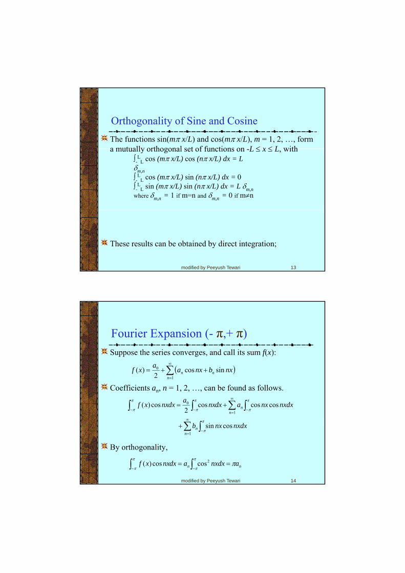
Orthogonality of Sine and CosineThe functions sin(mπ x/L) and cos(mπ x/L), m = 1, 2, …, form a mutually orthogonal set of functions on L ≤ x ≤ L witha mutually orthogonal set of functions on -L ≤ x ≤ L, with

∫-L

L cos (mπ x/L) cos (nπ x/L) dx = L δm,n∫-

LL cos (mπ x/L) sin (nπ x/L) dx = 0

∫-L

L sin (mπ x/L) sin (nπ x/L) dx = L δm,nwhere δm,n = 1 if m=n and δm,n = 0 if m≠n


These results can be obtained by direct integration;

Fourier Expansion (- π,+ π)Suppose the series converges, and call its sum f(x):

Coefficients an, n = 1, 2, …, can be found as follows.

( )∑∞

=

++=1

0 sincos2

)(n

nn nxbnxaaxf

∫∑

∫∑∫∫∞

−

∞

=−−

+=

π

π

π

π

π

π

π

db

nxdxnxadxnxadxnxxfn

n

i

coscoscos2

cos)(1

0


By orthogonality,

∫∑ −=

+π

nxdxnxbn

n cossin1

nn anxdxadxnxxf ππ

π

π

π== ∫∫ −−

2coscos)(

9/17/2009

8

Coefficient FormulasThus from the previous slide we have

1

To find the coefficient a0, we have

Thus the coefficients an are given by

011

0 sincos2

)( anxdxbnxdxadxadxxfn

nn

n ππ

π

π

π

π

π

π

π=++= ∫∑∫∑∫∫ −

∞

=−

∞

=−−

K,2,1,cos)(1== ∫− ndxnxxfan

π

ππ


Similarly, the coefficients bn are given by

K,2,1,0,cos)(1== ∫− ndxnxxfan

π

ππ

K,2,1,sin)(1== ∫− ndxnxxfbn

π

ππ

The Euler-Fourier Formula(- π,+ π)Thus the coefficients are given by the equations

1

which known as the Euler-Fourier formulas.Note that these formulas depend only on the values of f(x) in the interval π ≤ x ≤ π Since each term of the Fourier series

,,2,1,sin)(1

,,2,1,0,cos)(1

K

K

==

==

∫

∫

−

−

ndxnxxfb

ndxnxxfa

n

n

π

π

π

π

π

π


the interval - π ≤ x ≤ π. Since each term of the Fourier series

is periodic with period 2pi, the series converges for all x when it converges in - π ≤ x ≤ π, and f is determined for all x by its values in - π ≤ x ≤ π.

∑∞

=⎟⎠⎞

⎜⎝⎛ ++=

1

0 sincos2

)(n

nn Lxnb

Lxnaaxf ππ

9/17/2009

9

Find the F S. to represent x-x2 from-pi to pi.

∑ ∑∞

=

∞

=

++=−=1 1

0 sincos2

)(21)(

n nnn nxbnxaaxxf π=

∫ ∫−−

−==π

π

π

π

πππ

dxxdxxfa )(211)(1

0


πππ

π

π

=⎥⎦

⎤⎢⎣

⎡−

−22

1 2xx

∫ ∫− −

−==π

π

π

π

πππ

nxdxxnxdxxfan cos)(211cos)(1

( ) cos)1(sin1⎥⎤

⎢⎡

⎟⎞

⎜⎛ −

πnxnx( )

[ ] 0021

2cos)1(s

2

==

−⎥⎥⎦⎢

⎢⎣

⎟⎟⎠

⎜⎜⎝

−−−=

π

ππ

π n

nxn

nxxna

nxdxxb n sin)(211

−= ∫π

ππ


( )

n

nnx

nnxx

n)1(

sin)1(cos21

2

2

−=

⎥⎦

⎤⎢⎣

⎡⎟⎠⎞

⎜⎝⎛ −

−−−

−=−

−∫

π

π

π

ππ

π

9/17/2009

10

Using coeff. Just obtainedWe get

∑ ∑∞

=

∞

=

++=1 1

0 sincos2

)(n n

nn nxbnxaaxf

∞ )1( nπ

we get,


∑∞

=

−+=

1sin)1(

2)(

nnx

nxf π

EX

Ans

Obtain the Fourier expansion of f(x)=e-ax in the interval (-π, π).

=

=−

=

⎥⎦

⎤⎢⎣

⎡−

==

−

−

−

−

−

−

∫

∫0

cos1

sinh2

11

nxdxea

aa

aee

aedxea

axn

aa

axax

ππ

π

ππ

π

ππ

π

π

π

π


{ }

⎥⎦

⎤⎢⎣

⎡+

−=

⎥⎦

⎤⎢⎣

⎡+−

+=

−

−

−∫

22

22

sinh)1(2

sincos1

naaa

nxnnxana

ea

n

ax

n

n

ππ

π

ππ

π

π

9/17/2009

11

∫−

−=π

ππnxdxeb ax

n sin1

=

{ }π

ππ−

−

⎥⎦

⎤⎢⎣

⎡−−

+= nxnnxa

naeb

ax

n cossin122


⎥⎦

⎤⎢⎣

⎡+

−= 22

sinh)1(2na

an n ππ

Hence the F. S. Expansion

∑∑∞

=

∞

= +−

++−

+=1

221

22 sin)1(sinh2cos)1(sinh2sinh)(n

n

n

n

nxna

nanxna

aaa

axf πππ

πππ

∞ )1(sinh2sinh nππ


∑= +

−+==

12 1

)1(sinh2sinh1)0(n n

fπ

ππ

π

9/17/2009

12

Example 1 function

f(x)=x2,-π<x< π, f is even so all bn=0,( ) n

n nxdxxfa

dxxdxxfdxxfa

,cos)(2

,322)(2)(1

0

0

22

00

=

====

∫

∫∫ ∫−

π

ππ

π

π

π

ππππ


( )nn

n

na

nnx

nnnx

nx

nnxxa

140

sin2cos2sin2

2

02

2

−+=

⎥⎦

⎤⎢⎣

⎡⎟⎠⎞

⎜⎝⎛ −+⎟

⎠⎞

⎜⎝⎛ −−=

π

π

Example 1 continues

Hence the Fourier series is given byg y

1111,0

,...4

4cos3

3cos2

2cos1

cos43

221)(

2

2222

22

⎥⎤

⎢⎡ +

=

⎥⎦⎤

⎢⎣⎡ −+−−==

π

π

x

xxxxxxf


,...432112 2222 ⎥⎦⎢⎣

−+−=

9/17/2009

13

∑= −

+=Nn n nxxSLetsdefine

2 cos)1(4)( π ∑=

+=n

N nxSLetsdefine

124

3)(

xxxS

xxS

2coscos4)(

cos43

)(

2

2

1

+

−=

π

π


xxxxxxxS

xxxS

5cos915cos

2544cos

413cos

942coscos4

3)(

2coscos43

)(

2

6

2

+−+−+−=

+−=

π

K


9/17/2009

14


Now coeff. in Fourier Expansion if (-L,L)Suppose the series converges, and call its sum f(x):

⎞⎛

The coefficients an, n = 1, 2, …, can be found as follows.

∑∞

=⎟⎠⎞

⎜⎝⎛ ++=

1

0 sincos2

)(n

nn Lxnb

Lxnaaxf ππ

∫∑

∫∑∫∫∞

−

∞

=−−

+=

L

L

Ln

n

L

L

L

L

dxnxnb

dxL

xnL

xnadxL

xnadxL

xnxf

ππ

ππππ

i

coscoscos2

cos)(1

0


By orthogonality,

∫∑ −=

+L

nn dx

Lxn

Lxnb ππ cossin

1

n

L

Ln

L

LLadx

Lxnadx

Lxnxf == ∫∫ −−

ππ 2coscos)(

9/17/2009

15

Coefficient FormulasThus from the previous slide we have

1

To find the coefficient a0, we have

Thus the coefficients an are given by

011

0 sincos2

)( LadxL

xnbdxL

xnadxadxxfL

Ln

n

L

Ln

n

L

L

L

L=++= ∫∑∫∑∫∫ −

∞

=−

∞

=−−

ππ

K,2,1,cos)(1== ∫− ndx

Lxnxf

La

L

Lnπ


Similarly, the coefficients bn are given by

K,2,1,0,cos)(1,)(10 === ∫∫ −−

ndxL

xnxfL

adxxfL

aL

Ln

L

L

π

K,2,1,sin)(1== ∫− ndx

Lxnxf

Lb

L

Lnπ

The Euler-Fourier FormulasThus the coefficients are given by the equations

1 L π

which known as the Euler-Fourier formulas.Note that these formulas depend only on the values of f(x) in the interval L ≤ x ≤ L Since each term of the Fourier series

,,2,1,sin)(1

,,2,1,0,cos)(1

K

K

==

==

∫

∫

−

−

ndxL

xnxfL

b

ndxL

xnxfL

a

L

Ln

L

Ln

π

π


the interval -L ≤ x ≤ L. Since each term of the Fourier series

is periodic with period 2L, the series converges for all x when it converges in -L ≤ x ≤ L, and f is determined for all x by its values in -L ≤ x ≤ L.

∑∞

=⎟⎠⎞

⎜⎝⎛ ++=

1

0 sincos2

)(n

nn Lxnb

Lxnaaxf ππ

9/17/2009

16

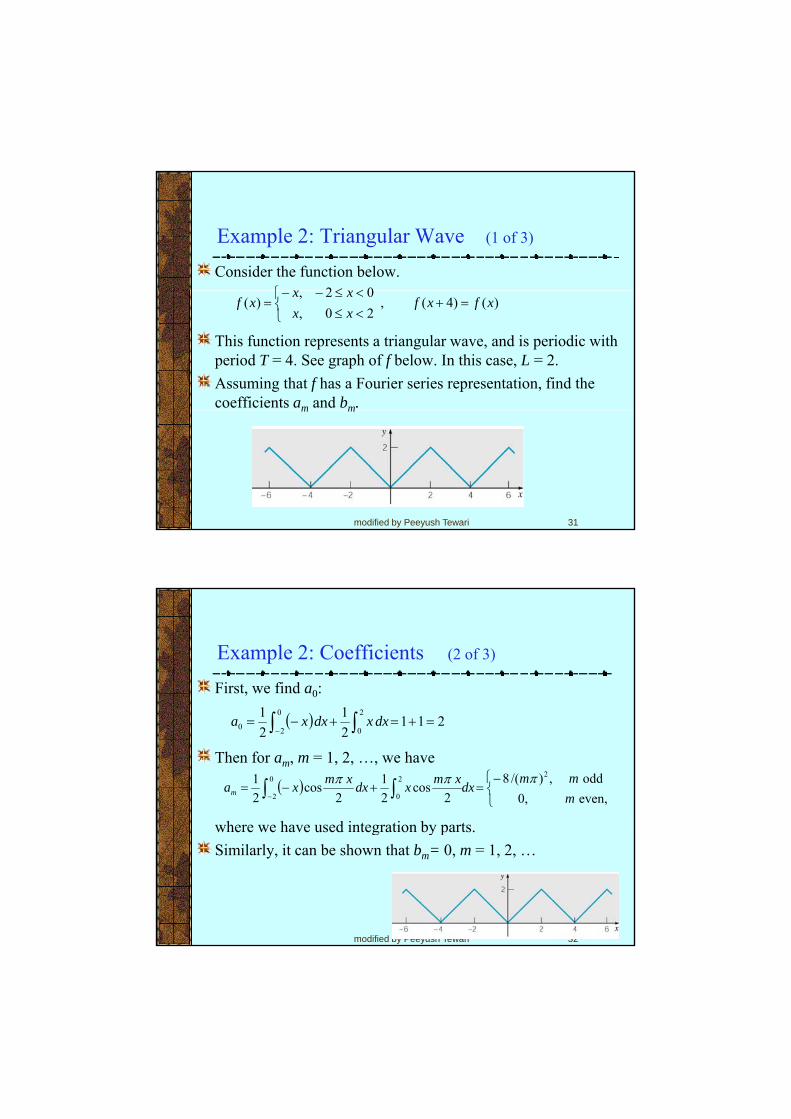
Example 2: Triangular Wave (1 of 3)

Consider the function below. 02 xx⎧ <≤

This function represents a triangular wave, and is periodic with period T = 4. See graph of f below. In this case, L = 2. Assuming that f has a Fourier series representation, find the coefficients am and bm.

)()4(,20,02,

)( xfxfxxxx

xf =+⎩⎨⎧

<≤<≤−−

=


m m

Example 2: Coefficients (2 of 3)

First, we find a0:11

Then for am, m = 1, 2, …, we have

where we have used integration by parts

( ) 21121

21 2

0

0

20 =+=+−= ∫∫− dxxdxxa

( )⎩⎨⎧−

=+−= ∫∫− even,0,odd,)/(8

2cos

21

2cos

21 22

0

0

2 mmm

dxxmxdxxmxamπππ


where we have used integration by parts. Similarly, it can be shown that bm= 0, m = 1, 2, …

9/17/2009

17

Example 2: Fourier Expansion (3 of 3)

Thus bm= 0, m = 1, 2, …, and⎧

Then

∑∞

=

⎟⎞

⎜⎛ +++−=

⎟⎠⎞

⎜⎝⎛ ++=

1

0

5cos13cos1cos81

sincos2

)(m

mm

xxxL

xmbL

xmaaxf

πππ

ππ

⎩⎨⎧−

==even,0,odd,)/(8

,22

0 mmm

aa mπ


∑

∑∞

=

∞

=

−−

−=

−=

⎟⎠

⎜⎝

+++−=

122

,...5,3,122

222

)12(2/)12cos(81

)2/cos(81

2cos

52cos

32cos1

n

m

nxn

mxm

ππ

ππ

πK

Example 3: Function (3 of 3)

Consider the function below. 130⎧

This function is periodic with period T = 6. In this case, L = 3. Assuming that f has a Fourier series representation, find the coefficients an and bn.

)()6(,31,011,113,0

)( xfxfxx

xxf =+

⎪⎩

⎪⎨

⎧

<<<<−−<<−

=


9/17/2009

18

Example 3: Coefficients (3 of 3)

First, we find a0:211

Using the Euler-Fourier formulas, we obtain32

31)(

31 1

1

3

30 === ∫∫ −−dxdxxfa

11

,,2,1,3

sin23

sin13

cos31

1

1

1

1

1K====

−−∫ nn

nxn

ndxxnan

ππ

ππ

π


,,2,1,03

cos13

sin31 1

1

1

1K==−==

−−∫ nxn

ndxxnbn

ππ

π

Example 3: Fourier Expansion (3 of 3)

Thus bn= 0, n = 1, 2, …, and

Then

+

⎟⎠⎞

⎜⎝⎛ ++=

∑

∑∞

∞

=

i21

sincos2

)(1

0

xnnL

xnbL

xnaaxfn

nn

ππ

ππ

K,2,1,3

sin2,32

0 === nnn

aa nπ

π


⎥⎦

⎤⎢⎣

⎡+⎟

⎠⎞

⎜⎝⎛−⎟

⎠⎞

⎜⎝⎛−⎟

⎠⎞

⎜⎝⎛+⎟

⎠⎞

⎜⎝⎛−=

+= ∑=

K3

5cos51

34cos

41

32cos

21

3cos3

31

3cos

3sin

3 1

xxxx

nn

πππππ

π

9/17/2009

19

Example 4: Triangular Wave Consider again the function from Example 1

02⎧ <≤

as graphed below, and its Fourier series representation

We now examine speed of convergence by finding the number

),()4(,20,02,

)( xfxfxxxx

xf =+⎩⎨⎧

<≤<≤−−

=

∑∞

= −−

−=1

22 )12(2/)12cos(81)(

n nxnxf π

π


We now examine speed of convergence by finding the number of terms needed so that the error is less than 0.01 for all x.

Example : Partial Sums The mth partial sum in the Fourier series is

and can be used to approximate the function f. The coefficients diminish as (2n -1)2, so the series converges fairly rapidly. This is seen below in the graph of s1, s2, and f.

,)12(

2/)12cos(81)(1

22 ∑= −

−−=

m

nm n

xnxs ππ


9/17/2009

20

Example : Errors To investigate the convergence in more detail, we consider the error function e (x) = f (x) s (x)error function em(x) = f (x) - sm(x). Given below is a graph of |e6(x)| on 0 ≤ x ≤ 2. Note that the error is greatest at x = 0 and x = 2, where the graph of f(x) has corners. Similar graphs are obtained for other values of m.


Example : Uniform Bound Since the maximum error occurs at x = 0 or x = 2, we obtain a uniform error bound for each m by evaluating |e (x)| at one ofuniform error bound for each m by evaluating |em(x)| at one of these points.For example, e6(2) = 0.03370, and hence |e6(x)| < 0.034 on 0 ≤ x ≤ 2, and consequently for all x.


9/17/2009

21

Example : Speed of Convergence The table below shows values of |em(2)| for other values of m, and these data points are plotted below alsoand these data points are plotted below also. From this information, we can begin to estimate the number of terms that are needed to achieve a given level of accuracy.To guarantee that |em(2)| ≤ 0.01, we need to choose m = 21.

m e_m(2)2 0 09937


2 0.099374 0.050406 0.03370

10 0.0202515 0.0135020 0.0101325 0.00810

At LastThanks .


fourier series and applications - tripod

Documents