four essays on modelling asset returns in the chinese ...etheses.bham.ac.uk/7655/1/wang17phd.pdf ·...
TRANSCRIPT
Four Essays on Modelling Asset Returns
in the Chinese Financial Market
by
Shixuan Wang
A thesis submitted to the University of Birmingham for the
degree of DOCTOR OF PHILOSOPHY
Department of Economics
Birmingham Business School
College of Social Science
University of Birmingham
March 2017

University of Birmingham Research Archive
e-theses repository This unpublished thesis/dissertation is copyright of the author and/or third parties. The intellectual property rights of the author or third parties in respect of this work are as defined by The Copyright Designs and Patents Act 1988 or as modified by any successor legislation. Any use made of information contained in this thesis/dissertation must be in accordance with that legislation and must be properly acknowledged. Further distribution or reproduction in any format is prohibited without the permission of the copyright holder.


ABSTRACT
Firstly, we employ a three-state hidden semi-Markov model (HSMM) to explain the
time-varying distribution of the Chinese stock market returns. Our results indicate that
the time-varying distribution depends on the hidden states, represented by three market
conditions, namely the bear, sidewalk, and bull markets.
Secondly, we further employ the three-state HSMM to the daily returns of the Chinese
stock market and seven developed markets. Through the comparison, three unique
characteristics of the Chinese stock market are found, namely “Crazy Bull”, “Frequent
and Quick Bear”, and “No Buffer Zone”.
Thirdly, we propose a new diffusion process referred to as the “camel process” to model
the cumulative return of a financial asset. Its steady state probability density function
could be unimodal or bimodal, depending on the sign of the market condition parameter.
The price reversal is realised through the non-linear drift term.
Lastly, we take the tools in functional data analysis to understand the term structure
of Chinese commodity futures and forecast their log returns at both short and long
horizons. The FANOVA has been applied to examine the calendar effect of the term
structure. An h-step functional autoregressive model is employed to forecast the log
return of the term structure.


Acknowledgements
First and foremost, I sincerely appreciate my supervisors, Prof Zhenya Liu and Prof
David Dickinson, for their academic guidance and incredible support during my PhD
study. Prof Liu taught me how to think independently and critically. Prof Dickinson
supported me without any reserve for all my academic activities. This thesis could not
be completed without their continuously generous help.
My deep gratitude goes to Prof Lajos Horvath and Dr William Pouliot. I learnt the way
of thinking in statistics from Prof Horvath. Dr Pouliot taught me how to perform Monte
Carlo simulation. The statistical knowledge I learnt from them greatly contributes to
this thesis.
My great appreciation goes to my parents who always supported and encouraged me in
every possible way for my life and studies. It is their unconditional love makes me move
forward. Additionally, my heartfelt thanks go to my girlfriend, Wan Li, who gave up
a comfortable life in China and chose to stay with me in the UK for a tough life. Her
countless praise on my research provides me energy to carry on in my dark time.
Last, but not least, I am grateful for the financial support from the Economic and
Social Research Council, UK, grant ES/J50001X/1 and a Royal Economic Society Junior
Fellowship.
v

Contents
Introduction 1
1 Decoding Chinese Stock Market Returns 17
1.1 Introduction . . . . . . . . . . . . . . . . . . . . . . . . . . . . . . . . . . . 18
1.2 Literature Review . . . . . . . . . . . . . . . . . . . . . . . . . . . . . . . 20
1.3 Data . . . . . . . . . . . . . . . . . . . . . . . . . . . . . . . . . . . . . . . 24
1.3.1 Data Information . . . . . . . . . . . . . . . . . . . . . . . . . . . . 24
1.3.2 Rationale for the CSI 300 . . . . . . . . . . . . . . . . . . . . . . . 24
1.4 Descriptive Statistics . . . . . . . . . . . . . . . . . . . . . . . . . . . . . . 25
1.5 Distributional and Temporal Properties . . . . . . . . . . . . . . . . . . . 26
1.5.1 Distributional Properties . . . . . . . . . . . . . . . . . . . . . . . 26
1.5.2 Temporal Properties . . . . . . . . . . . . . . . . . . . . . . . . . . 27
1.6 Methodology . . . . . . . . . . . . . . . . . . . . . . . . . . . . . . . . . . 31
1.6.1 Hidden Semi-Markov Model . . . . . . . . . . . . . . . . . . . . . . 31
1.6.2 Definition of Market Conditions . . . . . . . . . . . . . . . . . . . . 33
1.7 Empirical Results . . . . . . . . . . . . . . . . . . . . . . . . . . . . . . . . 35
1.7.1 Estimation Results . . . . . . . . . . . . . . . . . . . . . . . . . . . 35
1.7.2 Decoding Results . . . . . . . . . . . . . . . . . . . . . . . . . . . . 38
1.8 Model Evaluation and Comparison . . . . . . . . . . . . . . . . . . . . . . 42
1.8.1 Comparison with Other Volatility Models . . . . . . . . . . . . . . 44
1.8.2 Comparison with the Hidden Markov Models . . . . . . . . . . . . 49
1.9 Trading Strategy . . . . . . . . . . . . . . . . . . . . . . . . . . . . . . . . 51
1.10 Conclusion . . . . . . . . . . . . . . . . . . . . . . . . . . . . . . . . . . . 52
Appendix 55
1.A EM Algorithm . . . . . . . . . . . . . . . . . . . . . . . . . . . . . . . . . 55
1.B Decoding Technique . . . . . . . . . . . . . . . . . . . . . . . . . . . . . . 57
1.B.1 Global Decoding . . . . . . . . . . . . . . . . . . . . . . . . . . . . 58
1.B.2 Local Decoding . . . . . . . . . . . . . . . . . . . . . . . . . . . . . 59
1.C Robustness Test of the Trading Strategy . . . . . . . . . . . . . . . . . . . 59
2 Understanding the Chinese Stock Market 63
2.1 Introduction . . . . . . . . . . . . . . . . . . . . . . . . . . . . . . . . . . . 64
2.2 Literature Review . . . . . . . . . . . . . . . . . . . . . . . . . . . . . . . 65
2.3 Definition of Bear, Sidewalk, and Bull . . . . . . . . . . . . . . . . . . . . 67
2.4 Empirical Results . . . . . . . . . . . . . . . . . . . . . . . . . . . . . . . . 69
2.4.1 Data Description . . . . . . . . . . . . . . . . . . . . . . . . . . . . 69
vii

viii CONTENTS
2.4.2 Component Distribution - Evidence of “Crazy Bull” . . . . . . . . 70
2.4.3 Sojourn Time - Evidence of “Frequent and Quick Bear” . . . . . . 71
2.4.4 Transition Probability Matrix - Evidence of “No Buffer Zone” . . . 72
2.5 Discussion and Policy Implications . . . . . . . . . . . . . . . . . . . . . . 74
2.5.1 “Crazy Bull” - Rational Security Analysis and Adjust InvestorStructure . . . . . . . . . . . . . . . . . . . . . . . . . . . . . . . . 75
2.5.2 “Frequent and Quick Bear” - Risk Management Tools . . . . . . . 75
2.5.3 “No Buffer Zone” - Restriction on Leverage . . . . . . . . . . . . . 76
2.6 Conclusion . . . . . . . . . . . . . . . . . . . . . . . . . . . . . . . . . . . 77
3 Asset Return & Camel Process 79
3.1 Introduction . . . . . . . . . . . . . . . . . . . . . . . . . . . . . . . . . . . 80
3.2 Literature Review . . . . . . . . . . . . . . . . . . . . . . . . . . . . . . . 82
3.3 The SDE and its properties . . . . . . . . . . . . . . . . . . . . . . . . . . 83
3.3.1 Steady State PDF . . . . . . . . . . . . . . . . . . . . . . . . . . . 84
3.3.2 Time Dependent PDF . . . . . . . . . . . . . . . . . . . . . . . . . 89
3.4 Empirical Study . . . . . . . . . . . . . . . . . . . . . . . . . . . . . . . . 92
3.4.1 Data . . . . . . . . . . . . . . . . . . . . . . . . . . . . . . . . . . . 92
3.4.2 Maximum Likelihood Estimator . . . . . . . . . . . . . . . . . . . 94
3.4.3 Estimation Result . . . . . . . . . . . . . . . . . . . . . . . . . . . 94
3.5 Conclusion . . . . . . . . . . . . . . . . . . . . . . . . . . . . . . . . . . . 95
Appendix 97
3.A Steady State Solution of the Fokker-Planck Equation . . . . . . . . . . . . 97
3.B Steady State PDF when α is zero . . . . . . . . . . . . . . . . . . . . . . . 99
4 Forecasting the Log Return of Term Structure 101
4.1 Introduction . . . . . . . . . . . . . . . . . . . . . . . . . . . . . . . . . . . 102
4.2 Data and Functional Descriptive Statistics . . . . . . . . . . . . . . . . . . 105
4.2.1 Term Structure . . . . . . . . . . . . . . . . . . . . . . . . . . . . . 107
4.2.2 Log Return of the Term Structure . . . . . . . . . . . . . . . . . . 107
4.2.3 Functional Descriptive Statistics . . . . . . . . . . . . . . . . . . . 109
4.3 FANOVA . . . . . . . . . . . . . . . . . . . . . . . . . . . . . . . . . . . . 112
4.4 h-step Functional Autoregressive Model . . . . . . . . . . . . . . . . . . . 119
4.4.1 Estimated Kernel . . . . . . . . . . . . . . . . . . . . . . . . . . . . 120
4.4.2 Predictive Factors . . . . . . . . . . . . . . . . . . . . . . . . . . . 121
4.4.3 Forecast Performance Evaluation . . . . . . . . . . . . . . . . . . . 123
4.5 Forecasting Performance . . . . . . . . . . . . . . . . . . . . . . . . . . . . 124
4.5.1 In-Sample Fitting . . . . . . . . . . . . . . . . . . . . . . . . . . . 125
4.5.2 Out-of-Sample Forecasting . . . . . . . . . . . . . . . . . . . . . . . 128
4.6 Conclusion . . . . . . . . . . . . . . . . . . . . . . . . . . . . . . . . . . . 129
Conclusions, Limitations and Future Research 135
Bibliography 141

List of Figures
1.1 CSI 300 and its Returns . . . . . . . . . . . . . . . . . . . . . . . . . . . . 19
1.3 ACF of Original Returns, Squared Returns, and Absolute Returns . . . . 30
1.2 Taylor Effect . . . . . . . . . . . . . . . . . . . . . . . . . . . . . . . . . . 31
1.4 Empirical and Component Density . . . . . . . . . . . . . . . . . . . . . . 37
1.5 CSI 300 and Market Conditions (Global Decoding) . . . . . . . . . . . . . 41
1.6 Daily Returns of CSI300 and Market Conditions (Global Decoding) . . . 41
1.7 Local Decoding . . . . . . . . . . . . . . . . . . . . . . . . . . . . . . . . . 41
1.8 QQ Plots of the Log Returns . . . . . . . . . . . . . . . . . . . . . . . . . 46
1.9 Standardized Residuals and their QQ Plots . . . . . . . . . . . . . . . . . 47
1.10 Empirical ACF and Model ACF . . . . . . . . . . . . . . . . . . . . . . . 49
1.11 Taylor Effect from Simulation . . . . . . . . . . . . . . . . . . . . . . . . . 50
1.12 Performance of the Simple Trading Strategy . . . . . . . . . . . . . . . . . 53
1.C.1Performance of the Simple Trading Strategy - Period 1 . . . . . . . . . . . 60
1.C.2Performance of the Simple Trading Strategy - Period 2 . . . . . . . . . . . 60
1.C.3Performance of the Simple Trading Strategy - Period 3 . . . . . . . . . . . 61
3.1 Market Condition Parameter α . . . . . . . . . . . . . . . . . . . . . . . . 86
3.2 Volatility Parameter β . . . . . . . . . . . . . . . . . . . . . . . . . . . . . 88
3.3 Drift Term . . . . . . . . . . . . . . . . . . . . . . . . . . . . . . . . . . . 88
3.4 Volatility Parameter γ . . . . . . . . . . . . . . . . . . . . . . . . . . . . . 89
3.5 Time Dependent PDF . . . . . . . . . . . . . . . . . . . . . . . . . . . . . 92
3.6 Time Dependent PDF Slices vs. Steady State PDF . . . . . . . . . . . . . 93
3.1 Cumulative Return of S&P 500 and CSI 300 . . . . . . . . . . . . . . . . . 95
3.B.1Steady State PDF when α is zero . . . . . . . . . . . . . . . . . . . . . . . 99
4.1 Term Structure (RB) . . . . . . . . . . . . . . . . . . . . . . . . . . . . . . 108
4.2 Log Return of the Term Structure (RB) . . . . . . . . . . . . . . . . . . . 108
4.3 Functional Mean and Functional Standard Deviation (Term Structure) . . 110
4.4 Functional Mean and Functional Standard Deviation (Log Return of theTerm Structure) . . . . . . . . . . . . . . . . . . . . . . . . . . . . . . . . 111
4.5 Correlation Functions (Term Structure) . . . . . . . . . . . . . . . . . . . 112
4.6 Correlation Functions (Log Return of the Term Structure) . . . . . . . . . 113
4.1 Mean Curves for JM (Demeaned for each year) . . . . . . . . . . . . . . . 118
4.2 Mean Curves for SR (Demeaned for each year) . . . . . . . . . . . . . . . 118
4.3 Mean Curves for RB (Demeaned for each month/week) . . . . . . . . . . 118
ix


List of Tables
1 Statistics of Stock Exchanges . . . . . . . . . . . . . . . . . . . . . . . . . 3
2 Market Value Distribution of A-Shares Investors . . . . . . . . . . . . . . 6
3 Investors Age Distribution . . . . . . . . . . . . . . . . . . . . . . . . . . . 7
1.1 Descriptive Statistics . . . . . . . . . . . . . . . . . . . . . . . . . . . . . . 25
1.2 Various Parametric Distribution Fittings . . . . . . . . . . . . . . . . . . 28
1.3 Component Distribution Parameters . . . . . . . . . . . . . . . . . . . . . 36
1.4 Frequency of Positive and Negative Returns . . . . . . . . . . . . . . . . . 36
1.5 Sojourn Information . . . . . . . . . . . . . . . . . . . . . . . . . . . . . . 37
1.6 Transition Probability Matrix . . . . . . . . . . . . . . . . . . . . . . . . . 38
1.7 Estimation for the SV Model . . . . . . . . . . . . . . . . . . . . . . . . . 45
1.8 Estimation for the tGARCH(1,1) . . . . . . . . . . . . . . . . . . . . . . . 45
1.9 Model Comparison with Hidden Markov Models . . . . . . . . . . . . . . 51
2.1 Component Distribution . . . . . . . . . . . . . . . . . . . . . . . . . . . . 71
2.2 One-Sample z-test . . . . . . . . . . . . . . . . . . . . . . . . . . . . . . . 71
2.3 Days, Times, and Average Sojourn . . . . . . . . . . . . . . . . . . . . . . 73
2.4 Transition Probability Matrix . . . . . . . . . . . . . . . . . . . . . . . . . 74
3.1 Estimation Result . . . . . . . . . . . . . . . . . . . . . . . . . . . . . . . 94
4.1 Top 10 Global Futures and Options Exchange . . . . . . . . . . . . . . . . 103
4.1 Commodity Futures Information . . . . . . . . . . . . . . . . . . . . . . . 106
4.1 FANOVA Results . . . . . . . . . . . . . . . . . . . . . . . . . . . . . . . . 117
4.1 Optimised Values of α× 1000 . . . . . . . . . . . . . . . . . . . . . . . . . 126
4.2 1-day-ahead Forecasting Results . . . . . . . . . . . . . . . . . . . . . . . 130
4.3 1-week-ahead Forecasting Results . . . . . . . . . . . . . . . . . . . . . . . 131
4.4 1-month-ahead Forecasting Results . . . . . . . . . . . . . . . . . . . . . . 132
4.5 1-quarter-ahead Forecasting Results . . . . . . . . . . . . . . . . . . . . . 133
xi


Introduction
In the introduction, we provide the background information about the Chinese stock mar-
ket, review the relevant finance theories, and present the research questions, motivations,
and contributions.
1

2 INTRODUCTION
In this collection of four loosely related essays, several advanced quantitative methods,
namely hidden semi-Markov model, diffusion process, and functional data analysis, have
been applied to understand and model the asset returns in the Chinese financial market.
Before the discussion on the technical detail of the statistical methods used in each chap-
ter, it is useful to provide general information about Chinese stock market. We present
basic statistics of the Chinese stock market, such as market capitalization, trading value,
and number of listed companies, along with the discussion of main stock market indices
in China. Compared with developed markets, the Chinese stock market has a number
of unique features, such as limited openness, heavy regulation, and individual investors
dominating structure. Those unique features are closely related to the quantitative
results from the statistical methods.
Additionally, it is worthwhile to review the relevant finance theories, including the effi-
cient market hypothesis (EMH), technical analysis, and behavioural finance. Although
this thesis does not focus on testing EMH, but the results from the statistical methods
can provide some evidence of inefficiency in the Chinese financial market. In Chapter
1, we model the CSI 300 returns by a three-state HSMM and design a simple trading
strategy to exploit the arbitrage opportunity in the inefficient market. Our findings
contribute to the literature of technical analysis that are on the disapproval side of
the EMH. Behavioural finance provides us a solid foundation to explain some results
in Chapter 1 and Chapter 2. For example, the disposition effect is the reason of our
finding “bull mixed with bear” during 2007. With the consideration of the price reversal
and the market conditions, Chapter 3 propose a new diffusion process referred to as the
“camel process” in order to model the cumulative return of a financial asset. In Chapter
4, we show the predicability of functional autoregressive models on the term structure of
commodity futures in China, which provide the evidence of inefficiency in the Chinese
commodity futures market as well.

INTRODUCTION 3
The Institutional Background
Overview on the Chinese Stock Market
In mainland China, there are two main stock exchanges, namely the Shanghai Stock
Exchange (SSE) and the Shenzhen Stock Exchange (SZSE). Table 1 lists the largest ten
stock exchanges in the world, ranked by market capitalization in April 2017. SSE and
SZSE are ranked at the 4th place and the 8th place, respectively. Although SSE is larger
than SZSE in terms of market capitalization, SZSE has more trading value and more
number of listed companies.
Table 1: Statistics of Stock Exchanges (April 2017)
Market Cap.
(USD millions)
Trading Value
(USD millions)
NO. of Listed Companies
Total Domestic Foreign
1. NYSE 20,134,573.8 1,174,981.3 2,294 1,806 4882. Nasdaq - US 8,626,325.5 838,643.7 2,895 2,511 3843. Japan Exchange Group Inc. 5,263,274.0 437,602.4 3,562 3,556 64. Shanghai Stock Exchange 4,354,737.9 617,076.6 1,264 1,264 05. LSE Group 3,926,537.1 167,447.9 2,492 2,046 4466. Euronext 3,902,057.1 148,905.5 1,279 1,106 1737. Hong Kong Exchanges and Clearing 3,557,033.5 114,339.9 2,020 1,915 1058. Shenzhen Stock Exchange 3,294,346.1 716,443.3 1,959 1,959 09. TMX Group 2,056,681.6 96,303.0 3,426 3,378 4810. BSE India Limited 1,946,001.7 11,411.5 5,823 5,822 1
Source: World Federation of Exchanges members, affiliates, correspondents and non-members.
In the two exchanges, the common shares are classified as A-shares and B-shares. A-
shares are denominated by local currency RMB and traded in RMB only by domestic
institutional and individual investors. B-shares is also denominated by RMB but traded
in foreign currencies (USD in SSE and Hong Kong dollar in SZSE) by licensed foreign
and domestic investors. It should be highlighted that A-shares take up the majority
(nearly 96%) of the whole market.
During the last two decade, China has developed multi-tier stock market, consisting
of main board, SME board, and ChiNext board. The main board in SSE and SZSE
lists companies with large capital size and stable profit. Established in May 2004, SME
board is primarily targeted to list small and medium size companies with stable revenue.
The main sector of companies listed in SME board is the manufacturing, accounting for
75% of the SME board. Launched in October 2009, ChiNext is positioned to serve

4 INTRODUCTION
innovative and fast-growing enterprises, especially high-tech firms. ChiNext aims to
encourage innovation and creativity. The financial requirements of listing in ChiNext
are less stringent than those of the main and SME boards. SZSE asserts that ChiNext is
not a “mini-board” and it is open to all enterprises size as long as they meet the listing
criteria.
There are several major Chinese stock market indices often used by academic research.
The SSE Composite Index is a capitalization-weighted index, which represents the over-
all market movement of all A-shares and B-shares companies listed on SSE. The SZSE
Component Index is a capitalization-weighted index, consisting of the 500 top com-
panies listed in SZSE A-shares. The CSI 300 (a.k.a SHZE 300) index is a free-float
capitalization-weighted index based on 300 A-shares stocks listed on both SSE and
SZSE. There are several SSE size indices, SSE 50, SSE 180, and SSE 380, respectively
representing the top 50, 180, 380 companies listed on SSE A-shares by free-float capi-
talization weight.
Among those market indices, the CSI 300 index is widely accepted as an overall repre-
sentation for the general movements of the China A-share markets (Yang et al., 2012;
Hou & Li, 2014). The index was jointly launched by the SSE and SZSE on April 8th
2005. The index is complied and published by the China Securities Index Company
Ltd. It is comprised of 300 large-capitalization and actively traded stocks, which covers
roughly 70% of total market capitalization of the two stock markets (Yang et al., 2012).
More importantly, the first Chinese stock market index futures contract is based on the
CSI 300 index, launched on April 16th 2010. Hence, we will use the CSI 300 index for the
overall perfomrance representation of the Chinese stock market throughout this thesis.
Features of the Chinese Stock Market
Compared with developed markets, there are several unique features of the Chinese stock
market. Firstly, the Chinese stock market is relatively isolated from the international
financial markets because of very limited openness to the international investors. There
are no foreign companies listed on SSE and SZSE (see Table1). The only channel for
INTRODUCTION 5
foreign investors is the qualified foreign institutional investors (QFII). However, the ap-
plication for the QFII license is strictly examined by the the China Securities Regulatory
Commission (CSRC). For the foreign investors with the QFII license, there are still a
number of restrictions on their investment behaviour in the Chinese stock market.
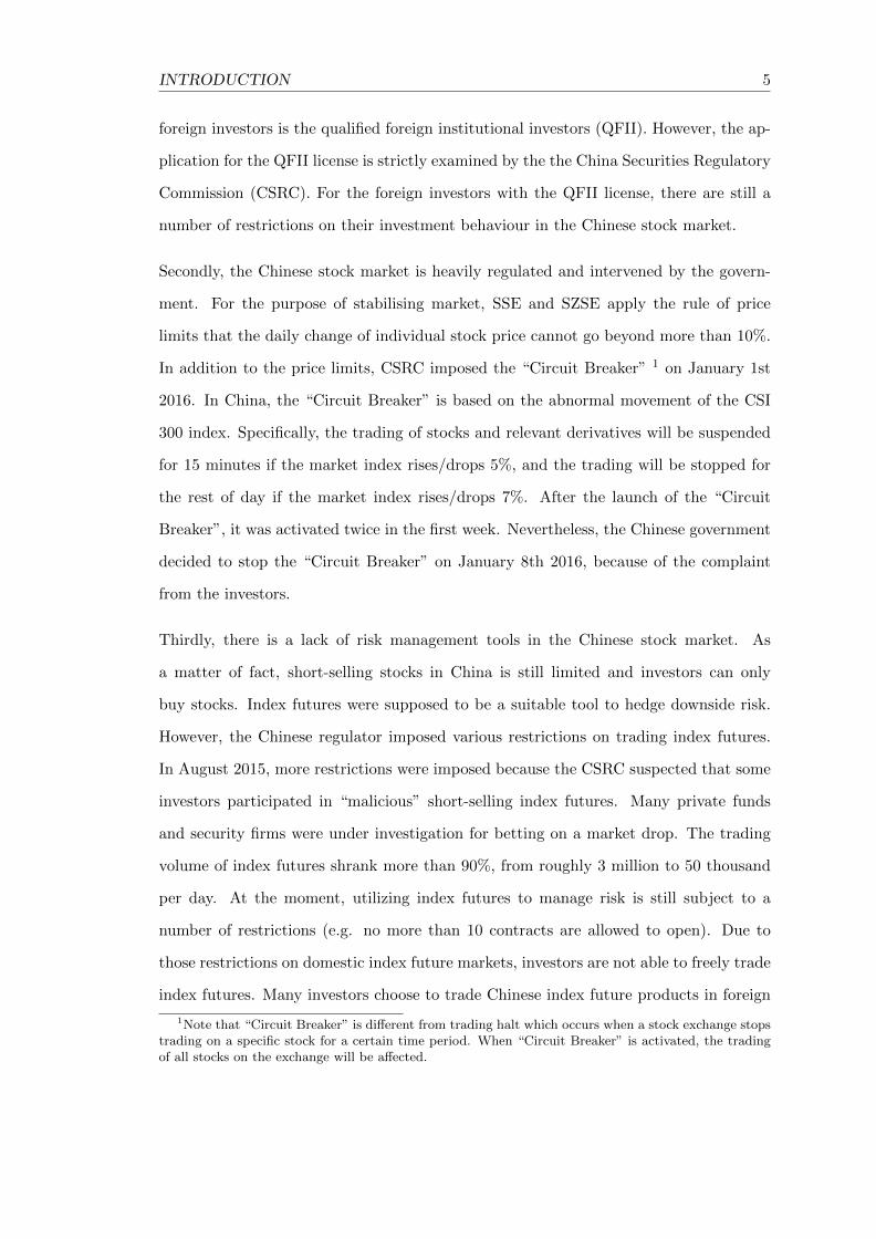
Secondly, the Chinese stock market is heavily regulated and intervened by the govern-
ment. For the purpose of stabilising market, SSE and SZSE apply the rule of price
limits that the daily change of individual stock price cannot go beyond more than 10%.
In addition to the price limits, CSRC imposed the “Circuit Breaker” 1 on January 1st
2016. In China, the “Circuit Breaker” is based on the abnormal movement of the CSI
300 index. Specifically, the trading of stocks and relevant derivatives will be suspended
for 15 minutes if the market index rises/drops 5%, and the trading will be stopped for
the rest of day if the market index rises/drops 7%. After the launch of the “Circuit
Breaker”, it was activated twice in the first week. Nevertheless, the Chinese government
decided to stop the “Circuit Breaker” on January 8th 2016, because of the complaint
from the investors.
Thirdly, there is a lack of risk management tools in the Chinese stock market. As
a matter of fact, short-selling stocks in China is still limited and investors can only
buy stocks. Index futures were supposed to be a suitable tool to hedge downside risk.
However, the Chinese regulator imposed various restrictions on trading index futures.
In August 2015, more restrictions were imposed because the CSRC suspected that some
investors participated in “malicious” short-selling index futures. Many private funds
and security firms were under investigation for betting on a market drop. The trading
volume of index futures shrank more than 90%, from roughly 3 million to 50 thousand
per day. At the moment, utilizing index futures to manage risk is still subject to a
number of restrictions (e.g. no more than 10 contracts are allowed to open). Due to
those restrictions on domestic index future markets, investors are not able to freely trade
index futures. Many investors choose to trade Chinese index future products in foreign
1Note that “Circuit Breaker” is different from trading halt which occurs when a stock exchange stopstrading on a specific stock for a certain time period. When “Circuit Breaker” is activated, the tradingof all stocks on the exchange will be affected.
6 INTRODUCTION
markets, like the FTSE China A50 index futures on the Singapore Exchange and E-mini
FTSE China 50 index futures on the Chicago Mercantile Exchange.
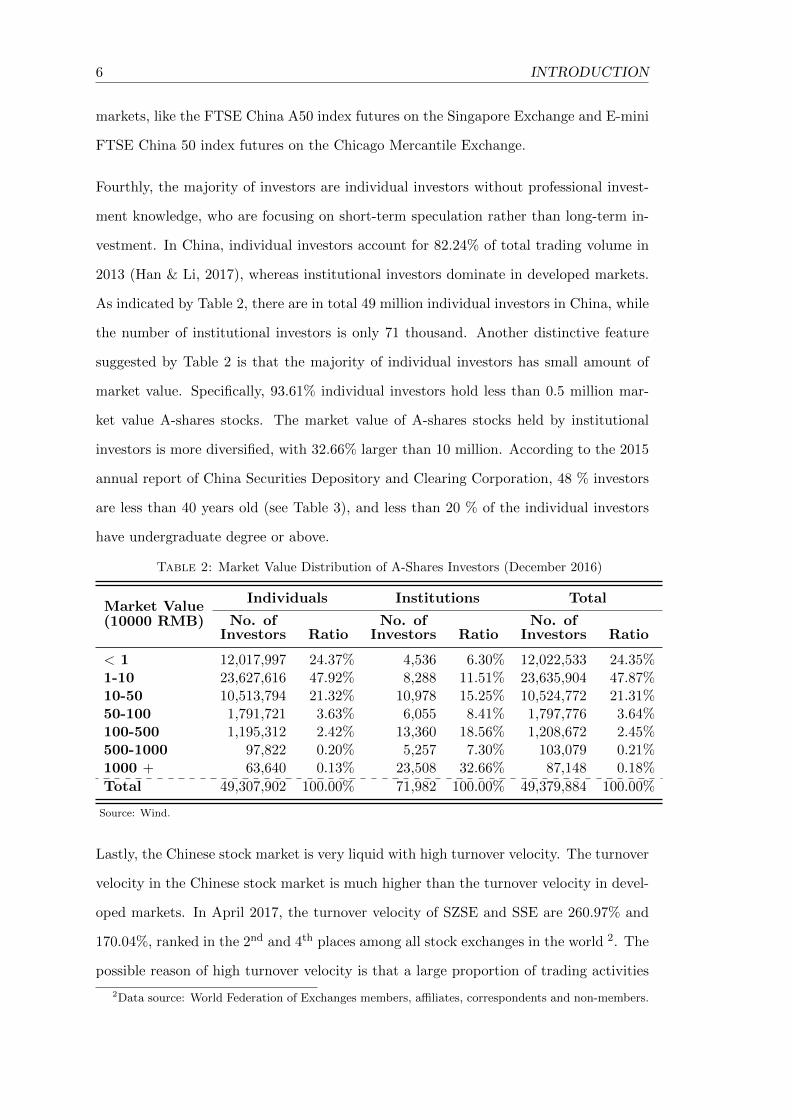
Fourthly, the majority of investors are individual investors without professional invest-
ment knowledge, who are focusing on short-term speculation rather than long-term in-
vestment. In China, individual investors account for 82.24% of total trading volume in
2013 (Han & Li, 2017), whereas institutional investors dominate in developed markets.
As indicated by Table 2, there are in total 49 million individual investors in China, while
the number of institutional investors is only 71 thousand. Another distinctive feature
suggested by Table 2 is that the majority of individual investors has small amount of
market value. Specifically, 93.61% individual investors hold less than 0.5 million mar-
ket value A-shares stocks. The market value of A-shares stocks held by institutional
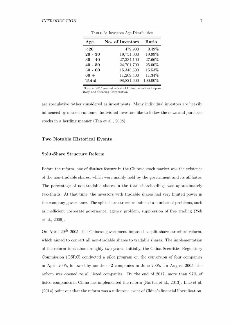
investors is more diversified, with 32.66% larger than 10 million. According to the 2015
annual report of China Securities Depository and Clearing Corporation, 48 % investors
are less than 40 years old (see Table 3), and less than 20 % of the individual investors
have undergraduate degree or above.
Table 2: Market Value Distribution of A-Shares Investors (December 2016)
Market Value(10000 RMB)
Individuals Institutions Total
No. ofInvestors Ratio
No. ofInvestors Ratio
No. ofInvestors Ratio
< 1 12,017,997 24.37% 4,536 6.30% 12,022,533 24.35%1-10 23,627,616 47.92% 8,288 11.51% 23,635,904 47.87%10-50 10,513,794 21.32% 10,978 15.25% 10,524,772 21.31%50-100 1,791,721 3.63% 6,055 8.41% 1,797,776 3.64%100-500 1,195,312 2.42% 13,360 18.56% 1,208,672 2.45%500-1000 97,822 0.20% 5,257 7.30% 103,079 0.21%1000 + 63,640 0.13% 23,508 32.66% 87,148 0.18%
Total 49,307,902 100.00% 71,982 100.00% 49,379,884 100.00%
Source: Wind.
Lastly, the Chinese stock market is very liquid with high turnover velocity. The turnover
velocity in the Chinese stock market is much higher than the turnover velocity in devel-
oped markets. In April 2017, the turnover velocity of SZSE and SSE are 260.97% and
170.04%, ranked in the 2nd and 4th places among all stock exchanges in the world 2. The
possible reason of high turnover velocity is that a large proportion of trading activities
2Data source: World Federation of Exchanges members, affiliates, correspondents and non-members.
INTRODUCTION 7
Table 3: Investors Age Distribution
Age No. of Investors Ratio
<20 479,900 0.49%20 - 30 19,751,000 19.99%30 - 40 27,334,100 27.66%40 - 50 24,701,700 25.00%50 - 60 15,345,500 15.53%60 + 11,209,400 11.34%Total 98,821,600 100.00%
Source: 2015 annual report of China Securities Depos-itory and Clearing Corporation.
are speculative rather considered as investments. Many individual investors are heavily
influenced by market rumours. Individual investors like to follow the news and purchase
stocks in a herding manner (Tan et al., 2008).
Two Notable Historical Events
Split-Share Structure Reform
Before the reform, one of distinct feature in the Chinese stock market was the existence
of the non-tradable shares, which were mainly held by the government and its affiliates.
The percentage of non-tradable shares in the total shareholdings was approximately
two-thirds. At that time, the investors with tradable shares had very limited power in
the company governance. The split-share structure induced a number of problems, such
as inefficient corporate governance, agency problem, suppression of free trading (Yeh
et al., 2009).
On April 29th 2005, the Chinese government imposed a split-share structure reform,
which aimed to convert all non-tradable shares to tradable shares. The implementation
of the reform took about roughly two years. Initially, the China Securities Regulatory
Commission (CSRC) conducted a pilot program on the conversion of four companies
in April 2005, followed by another 42 companies in June 2005. In August 2005, the
reform was opened to all listed companies. By the end of 2017, more than 97% of
listed companies in China has implemented the reform (Nartea et al., 2013). Liao et al.
(2014) point out that the reform was a milestone event of China’s financial liberalization,

8 INTRODUCTION
which significantly reduced agency problems and improved the corporate governance of
the listed companies. Due to the conversion from non-tradable shares to tradable shares,
the reform had provided substantial liquidity to the market.
Other Source Financing
It has been observed that other source financing activities are very active during 2015.
Other source financing refers to borrow funds from trust companies, fund-matching com-
panies, etc. Unlike margin loan and margin financing, the regulation on other source
financing is much less strict, which would be essential cause for the high leverage. For
example, umbrella trusts are not required to register with the China Securities Depos-
itory and Clearing Corporation. Umbrella trusts contain two sorts of tranches. Banks
purchase the senior tranches, which guarantee fixed returns. Subordinate tranches are
sold to private clients, like wealthy individuals, private companies, and fund-matching
companies, and provide uncertain returns depending on the performance of the wealth
management product. In other words, subordinate tranches would get the rest of invest-
ment profits. Jiang (2014) claimed that the Minsheng Bank, China Everbright Bank,
and China Merchants Bank were heavily involved in the business of umbrella trusts.
There is no accurate data about the size of umbrella trusts but some estimations indi-
cate that they accounted for roughly 200 billion RMB by the end of 2014 (Hsu, 2015).
In favour of high interest rates, fund-matching companies lend funds to investors by
providing margin loans without sufficient consideration of risk. Yap (2015) pointed out
that fund-matching companies channelled 500 billion RMB (June 30, 2015) from open-
ing multiple and subdivided securities accounts with brokerages. These fund-matching
companies were subject to a lack of regulation until CSRC imposed restrictions on them
in July 2015.
INTRODUCTION 9
Theoretical Background
The Efficient Market Hypothesis and Anomalies
One of most relevant finance theory is the efficient market hypothesis (EMH). The
widely accepted definition of the EMH is proposed by Fama (1970). He defines the EMH
as that “A market in which prices always ‘fully reflect’ available information is called
‘efficient’ ”. He further distinguishes three different forms of the EMH, namely weak
form, semi-strong form, and strong form, depending on the information set of historical
prices only, public available information, any relevant information, respectively.
In the 1970s, the EMH was generally accepted by the academic researches in financial
economics (Shiller, 2003). One straightforward implication of the EMH is that the
future stock price is unpredictable. Fama (1965) concludes that the stock price follows a
random walk with empirical evidence from the thirty stocks of the Dow-Jones Industrial
Average. He verifies the random walk model by separately testing two sub-hypotheses
that the successive price changes are independent and the price changes follow some
probability distribution. Samuelson (1965) uses a concept of the martingale to prove
that anticipated prices fluctuate randomly. The random walk model and the martingale
hypothesis severely challenge the proponents of the technical analysis, which will be
discussed in depth later.
After the prevalence of the EMH, many researchers in finance and statistics, however,
started to doubt the EMH and believe that the stock prices are at least partially predi-
cable (Malkiel, 2003). From the time-series perspective, Campbell et al. (1997) and Lo
& MacKinlay (2002) find the short-term momentum that the stocks with short-term (i.e.
daily, weakly, and monthly) above-average returns tend to have a high probability of
further above-average returns in the subsequent period, which is the evidence rejecting
the EMH in the sense that the stock price is not purely random walk. But only 12
percent of the variation in the daily stock market index can be predicted by using the
information of the past daily returns (Beechey et al., 2000). At longer horizons (three to
fives years), many studies have shown evidence of mean reversion in stock returns (e.g.
Fama & French, 1988; Poterba & Summers, 1988). Fama & French (1988) claim that

10 INTRODUCTION
20 to 40 percent of the variation in the long horizon returns can be predicted by using
the information of the past returns.
There are some other anomalies from the cross-sectional perspective, such as the size
effect, the value effect, etc. Fama & French (1993) identify that the small-capitalization
company stocks tend to have larger returns than those of large-capitalization company
stocks and that stocks of companies with high book-to-market ratio (i.e. high value)
tend to have larger returns than ones with low book-to-market ratio. They further
conclude that the size and the value together can provide explanatory power for stock
returns.
A number of researches have found the calender effects of stock returns, such as month-
of-the-year and day-of-the-week effects, which uncover the empirical evidence that the
average stock returns in a certain calender month or weekday appear to be significantly
different from the other months or weekdays. For example, Haugen & Lakonishok (1988)
find the relatively higher returns in January (the January effect), and French (1980)
documents the significantly higher returns on Monday (the weekend effect). However,
Malkiel (2003) claims that these calender effects are comparatively small to the trans-
actions costs when someone actually exploit them in practice.
Due to the joint hypothesis problem indicated by Campbell et al. (1997), the market
efficiency is empirically rejected could be because the market is truly inefficient or be-
cause the wrong market equilibrium is assumed. In this sense, the EMH is not testable.
Throughout this thesis, we focus on the statistical methods in terms of measuring effi-
ciency rather than testing the EMH.
Technical Analysis
Technical analysis, also known as “charting”, is to predict the future price movement
by identifying the presence of geometric shapes in historical price charts, sometimes
also with information of volume and open interest. Under the EMH, the current price
has already reflected all past available information, which naturally has the implication

INTRODUCTION 11
that technical analysis should provide no useful information for forecasting future price
movement (Fama, 1965).
Nevertheless, technical analysis has been widely used by traders in practice. For example,
more than 90 percent of foreign exchange traders in the London market performed one
to four weeks ahead forecasting by technical analysis in 1990s (Allen & Taylor, 1990).
It has been a long-standing debate on the usefulness of technical analysis in academia.
One difficulty of technical analysis is that the geometric shapes are sometimes difficult
to be mathematically define.
The empirical studies show the mixed results whether technical analysis can generate
excess returns. On the approval side, a number of studies have found the evidence of
excess returns generated by technical analysis (e.g. Pruitt & White, 1988; Brock et al.,
1992; Neely et al., 1997; Coutts & Cheung, 2000; Leigh et al., 2002; Okunev & White,
2003). In particular, Lo et al. (2000) employ kernel smoothing technique to automatically
recognise ten sophisticated technical charts, such as Head-and-Shoulders, Broadening,
and Triangle, and further find several technical indicators do have predictive power.
However, some studies suspected the validity of technical analysis because of the data
mining problem (e.g. Brock et al., 1992).
On the disapproval side, many researchers show that technical analysis does not out-
perform simple buy-and-hold strategy (e.g. Curcio et al., 1997; Hamm & Wade Brorsen,
2000; Lucke, 2003). Other studies find that the profits from the technical analysis de-
clines over time (e.g. Guillaume, 2012). In particular, Coutts (2010) re-examines the
trading rules in Coutts & Cheung (2000) with a more updated sample period and con-
cludes that those trading rules become defunct.
Behavioural Finance
In the 1990s, the theories of behavioural finance were developed to explain why and
how financial markets might be inefficient. Shiller (2003) defines behavioural finance
as “finance from a broader social science perspective including psychology and sociol-
ogy”. The key assumption in behavioural finance is that not all investors are rational,

12 INTRODUCTION
and those irrational investors (often known as noise traders) make the asset prices de-
viate from their fundamental values. The irrational behaviour comes from a number of
human psychological activities, including overconfidence, myopic loss aversion, represen-
tativeness, conservatism, belief perseverance, anchoring, and availability biases. Those
psychological activities impede investors to form the correct expectation on the asset
prices and to further conduct irrational investment decisions.
Two phenomena often discussed by behavioural finance are overreaction and underre-
action, which refer to that the investors react disproportionately to new information.
DeBondt & Thaler (1985) find that most investors usually overreact to unexpected and
dramatic news, suggesting the weak from market inefficiencies. De Bondt & Thaler
(1987) further find additional evidence to support the overreaction hypothesis, which
contradicts two alternative hypotheses based on the size of company and risk difference.
It is not always overreaction, but sometimes be slow or underreaction. Hong & Stein
(1999) construct a model with two groups of boundedly rational agents “newwatchers”
and “momentum traders” and show the underreaction at short horizons and overreaction
at long horizons. Fama (1998) claims that overreaction to information is as frequent as
underreaction. Veronesi (1999) uses a dynamic, rational expectations equilibrium model
of asset prices to demonstrate that stock prices underreact to good news in bad times
and overreact to bad news in good times. Farag (2014) use the system GMM to find
strong evidence of price reversal after the overreaction in the Egyptian stock market.
The disposition effect is the phenomena that investors tend to sell assets that have
gained profit (“winners”) and hold assets that have lost value (“losers”). Weber &
Camerer (1998) conduct experiments and find that the experimental subjects did tend
to sell winners and keep losers, which can be explained by the multiple reference points
affecting framing and guide choices. Barber & Odean (1999) study the disposition
effect and concludes that overconfidence is the possible reason. Barberis & Xiong (2009)
investigate the driving reason for the disposition effect and conclude that the model with
preferences defined over annual gains and losses fails to predict the disposition effect but
the model with preferences defined over realized gains and losses predicts the disposition
effect more reliably.
INTRODUCTION 13
Behavioural finance is applied to explain the excess returns of some trading strate-
gies. Lakonishok et al. (1994) investigate the reason for the higher returns of the value
strategies and find that these strategies exploit the suboptimal behaviour of the typi-
cal investor. Chan et al. (1996) explain the profitability of the momentum strategies
as that the market responds gradually to new information, i.e. there is underreaction.
Lee & Swaminathan (2000) discover an important link between momentum and value
strategies is the past trading volume, and their findings helps to intermediate-horizon
underreaction and long-horizon overreaction effects. Apart from explanation using be-
havioural finance, Frazzini (2006) designs a even-driven trading strategy based on the
disposition effect and this trading strategy generates monthly alphas of over 200 basis
points.
Research Questions, Motivations, and Contributions
In this collection of four loosely related essays, namely several quantitative methods,
hidden semi-Markov model, diffusion process, and functional data analysis, have been
applied to understand and model the asset returns in the Chinese financial market.
HSMM is a generalisation of the HMM by explicitly specifying the sojourn time dis-
tribution (Yu, 2010). Bulla & Bulla (2006) examine the reproduction of the stylized
facts of the asset returns by the US industry stock indices and show that HSMM is
superior to HMM because the stylized facts of the daily returns were entirely repro-
duced. Due to the merits of HSMM in the literature, we employ a three-state HSMM
to decode the Chinese stock market returns in Chapter 1. Firstly, it is appropriate to
employ a three-state HSMM to explain the time-varying distribution of Chinese stock
market returns. Secondly, the hidden states in the HSMM correspond to the market
conditions, namely the bear, sidewalk, and bull market. Unlike the definition of market
conditions in the literature (Fabozzi & Francis, 1977; Chauvet & Potter, 2000; Edwards
& Caglayan, 2001; Lunde & Timmermann, 2004; Gonzalez et al., 2006; Cheng et al.,
2013), we provide a systematic way to find the timing of three-category classification,
namely the bull, sidewalk, and bear market, for the daily data. Thirdly, we show the

14 INTRODUCTION
inefficiency of the market by design a trading strategy based on the expanding window
decoding. The trading strategy generates risk-adjusted return with a Sharpe ratio of
1.14 in the testing sample.
The by-product of Chapter 1 is our statistical definition of market conditions, i.e. bear,
sidewalk, and bull markets, which correspond to the three states in the HSMM. As
discussed above, the regulation and the investor structure of the Chinese stock market
are different from the developed markets. It is natural to question the difference in
terms of market conditions between the Chinese stock market and developed market. In
Chapter 2, we employ the three-state HSMM to the daily returns of the Chinese stock
market and the other seven developed markets. Using the Viterbi algorithm to globally
decode the most likely sequence of the market conditions, we systematically find the
precise timing of bear, sidewalk, and bull markets for all eight markets. Through the
comparison of the estimation and decoding results, many unique characteristics of the
market conditions in China are found, such as “Crazy Bull”, “Frequent and Quick Bear”,
and “No Buffer Zone”. In China, the bull market is more volatile than in developed
markets, the bear market occurs more frequently than in developed markets, and the
sidewalk market has not functioned as a buffer zone since 2005. Lastly, possible causes of
the unique characteristics are discussed and implications for policy-making are suggested.
As indicated in the first two chapters, the asset returns behaves differently in different
market conditions. Additionally, the overreaction has been widely studied in behavioural
finance. To the best of our knowledge, there is no diffusion process considering both
market condition and overreaction. In Chapter 3, we propose a new diffusion process
referred to as the “camel process” in order to model the cumulative return of a financial
asset. The process considers the market condition and the price reversal. This new
process includes three parameters, the market condition parameter α, the overreaction
correction parameter β, and the volatility parameter γ. Its steady state probability
density function could be unimodal or bimodal, depending on the sign of the market
condition parameter. The price reversal is realised through the non-linear drift term
which incorporates the cube term of the instantaneous cumulative return. The time-
dependent solution of its Fokker-Planck equation cannot be obtained analytically, but

INTRODUCTION 15
can be numerically solved using the finite difference method. The properties of the camel
process are confirmed by our empirical estimation results of ten market indexes in two
different periods. The nature of the research in Chapter 3 is more theoretical rather
than empirical.
In the last chapter, we shift from the stock market to the commodity futures market
because the stringent constraints on short selling stocks make it very difficult to manage
the downside risk and investing in commodity futures is an effect way to diversify against
falling stock prices (Edwards & Caglayan, 2001; Jensen et al., 2002; Wang & Yu, 2004;
Erb & Harvey, 2006). We should not restrict ourselves only in the stock market, and
it is worthwhile and meaningful to investigate the commodity futures market in China.
Chapter 4 takes the tools in functional data analysis to understand the term structure of
Chinese commodity futures and forecast their log returns at both short and long horizons.
A functional ANOVA (FANOVA) has been applied in order to examine the calendar
effect of the term structure. We use an h-step Functional Autoregressive model to
forecast the log return of the term structure. Compared with the naive predictor, the in-
sample and out-of-sample forecasting performance indicates that additional forecasting
power is gained by using the functional autoregressive structure. Although the log return
at short horizons is not predictable, the forecasts appear to be more accurate at long
horizons due to the stronger temporal dependence. The predictive factor method has
a better in-sample fitting, but it cannot outperform the estimated kernel method for
out-of-sample testing, except in the case of 1-quarter-ahead forecasting.

Chapter 1
Decoding Chinese Stock Market Returns:
Three-State Hidden Semi-Markov Model, Market
Conditions, and Market Inefficiency
In this chapter, we employ a three-state hidden semi-Markov model (HSMM) to explain
the time-varying distribution of the Chinese stock market returns since 2005. Our re-
sults indicate that the time-varying distribution depends on the hidden states, which are
represented by three market conditions, namely the bear, sidewalk, and bull markets. In
order to show the inefficiency of the market, we design a simple trading strategy based
on expanding window decoding that generates risk-adjusted return with a Sharpe ratio of
1.14.
17
18 Chapter 1 Decoding Chinese Stock Market Returns
1.1 Introduction
The term “decoding”, originally from the field of speech recognition, is the procedure of
deciphering observations into the underlying pattern that drives the mechanism. In this
chapter, we aim to decode the Chinese stock market returns through a new developed
statistical model, namely hidden semi-Markov Model (HSMM). More specifically, we are
going to answer three questions: 1) can we use the HSMM to explain the time-varying
distribution of the Chinese stock market returns? 2) what is the economic interpretation
of the hidden states in the HSMM? 3) can we design a profitable trading strategy based
on the HSMM to show the inefficiency of the market?
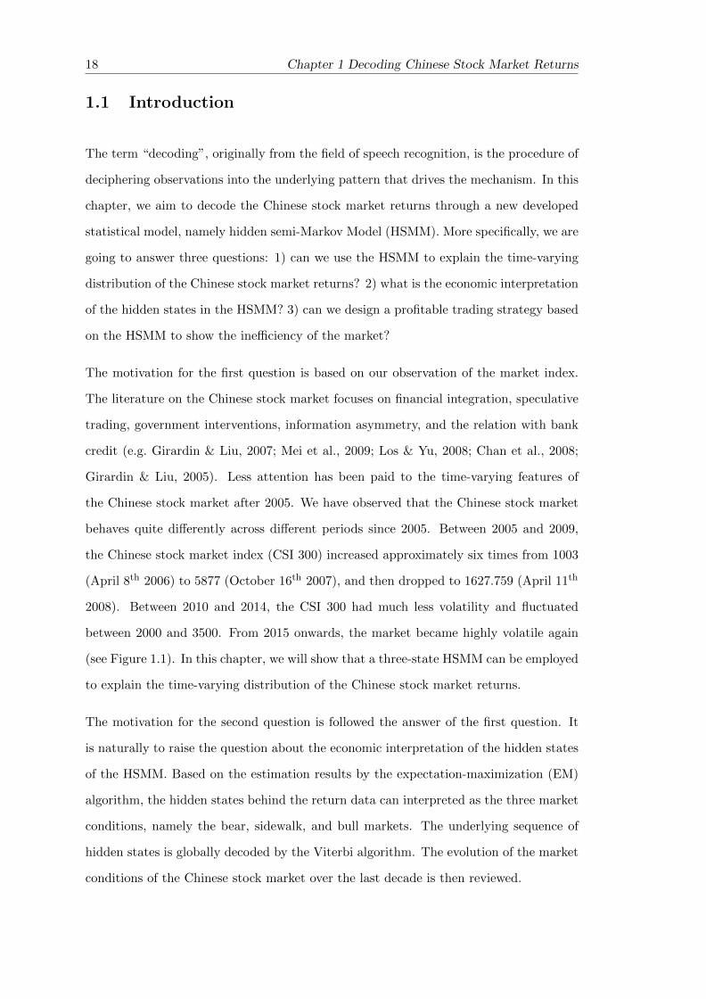
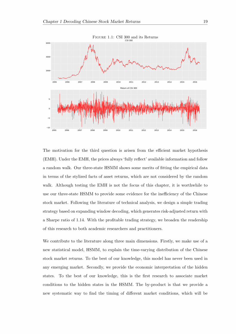
The motivation for the first question is based on our observation of the market index.
The literature on the Chinese stock market focuses on financial integration, speculative
trading, government interventions, information asymmetry, and the relation with bank
credit (e.g. Girardin & Liu, 2007; Mei et al., 2009; Los & Yu, 2008; Chan et al., 2008;
Girardin & Liu, 2005). Less attention has been paid to the time-varying features of
the Chinese stock market after 2005. We have observed that the Chinese stock market
behaves quite differently across different periods since 2005. Between 2005 and 2009,
the Chinese stock market index (CSI 300) increased approximately six times from 1003
(April 8th 2006) to 5877 (October 16th 2007), and then dropped to 1627.759 (April 11th
2008). Between 2010 and 2014, the CSI 300 had much less volatility and fluctuated
between 2000 and 3500. From 2015 onwards, the market became highly volatile again
(see Figure 1.1). In this chapter, we will show that a three-state HSMM can be employed
to explain the time-varying distribution of the Chinese stock market returns.
The motivation for the second question is followed the answer of the first question. It
is naturally to raise the question about the economic interpretation of the hidden states
of the HSMM. Based on the estimation results by the expectation-maximization (EM)
algorithm, the hidden states behind the return data can interpreted as the three market
conditions, namely the bear, sidewalk, and bull markets. The underlying sequence of
hidden states is globally decoded by the Viterbi algorithm. The evolution of the market
conditions of the Chinese stock market over the last decade is then reviewed.
Chapter 1 Decoding Chinese Stock Market Returns 19
Figure 1.1: CSI 300 and its Returns
2000
4000
6000
2005 2006 2007 2008 2009 2010 2011 2012 2013 2014 2015 2016
CSI 300
−10
−5
0
5
2005 2006 2007 2008 2009 2010 2011 2012 2013 2014 2015 2016
Return of CSI 300
The motivation for the third question is arisen from the efficient market hypothesis
(EMH). Under the EMH, the prices always ‘fully reflect’ available information and follow
a random walk. Our three-state HSMM shows some merits of fitting the empirical data
in terms of the stylized facts of asset returns, which are not considered by the random
walk. Although testing the EMH is not the focus of this chapter, it is worthwhile to
use our three-state HSMM to provide some evidence for the inefficiency of the Chinese
stock market. Following the literature of technical analysis, we design a simple trading
strategy based on expanding window decoding, which generates risk-adjusted return with
a Sharpe ratio of 1.14. With the profitable trading strategy, we broaden the readership
of this research to both academic researchers and practitioners.
We contribute to the literature along three main dimensions. Firstly, we make use of a
new statistical model, HSMM, to explain the time-varying distribution of the Chinese
stock market returns. To the best of our knowledge, this model has never been used in
any emerging market. Secondly, we provide the economic interpretation of the hidden
states. To the best of our knowledge, this is the first research to associate market
conditions to the hidden states in the HSMM. The by-product is that we provide a
new systematic way to find the timing of different market conditions, which will be

20 Chapter 1 Decoding Chinese Stock Market Returns
used in Chapter 2. Thirdly, we contribute to the literature of technical trading rules by
proposing a new profitable trading strategy based on our model.
The remainder of the chapter is structured as follows. Section 1.2 reviews the literature
of relevant studies. Section 1.3 describes our data and its descriptive statistics. Section
1.6 briefly introduces the HSMM, estimation method, decoding techniques and our model
set-up. In Section 1.7, the estimation results and the decoding results are presented and
their economic meanings are discussed, followed by the model evaluation and comparison
in Section 1.8. Section 1.9 presents a simple trading strategy with a Sharpe ratio of 1.14.
Section 1.10 summarises the chapter.
1.2 Literature Review
Stylized Facts of Asset Returns
The stylized facts of asset returns in the developed markets are well documented in the
literature (Granger & Ding, 1995; Pagan, 1996; Cont, 2001). They can be classified
into two categories, namely distributional properties and temporal properties. Distri-
butional properties relate to the non-Gaussianity of the distribution of asset returns,
whilst temporal properties refer to the time dependence of asset returns and of the
squared/absolute asset returns.
In the early studies exploring distributional properties, normal distributions with sta-
tionary parameters were often selected in order to model daily asset returns. However,
Mandelbrot (1997) doubted the Gaussian hypothesis of asset returns and stated that sta-
ble Paretian distributions with characteristic exponents of less than 2 are better suited to
fit the empirical distribution of assets (Mandelbrots hypothesis). Fama (1965) undertook
extensive testing on empirical data and found that extreme tail values are more frequent
than the Gaussian hypothesis (a.k.a. leptokurtosis), which supports the Mandelbrots
hypothesis. In order to explain the notion of leptokurtosis, Fama tried two modified ver-
sions of the Gaussian model: a Gaussian mixture model and a non-stationary Gaussian
model. However, his empirical evidence supports neither of them. Praetz (1972) and

Chapter 1 Decoding Chinese Stock Market Returns 21
Blattberg & Gonedes (1974) employed t-distributions with small degrees of freedom in
order to capture the fat-tail of the empirical distribution of asset returns. Granger &
Ding (1995) suggested that the appropriate distribution is the double exponential dis-
tribution with zero mean and unit variance. Mittnik & Rachev (1993) inspected various
stable distributions for asset returns and found that the Weibull distribution gave the
best fit for the S&P 500 daily returns between 1982 and 1986.
In terms of temporal properties, the ARCH-family models are often used for volatility
clustering. The original ARCH model was introduced by Engle (1982) in order to model
non-constant variances. Bollerslev (1986) generalised the ARCH model by allowing
past conditional variances to affect current conditional variances. Afterwards, variants
of the GARCH were developed, including EGARCH, GJR, GARCH-M, and so forth.
Bollerslev et al. (1992) comprehensively reviewed many types of GARCH models. As for
the continuous-time set-up, stochastic volatility models were introduced by Taylor (1986)
in an attempt to overcome the main drawback of the Black-Scholes model characterised
by a constant volatility. Stochastic volatility models facilitate analysis of a variety of
option pricing problems. A review of the stochastic volatility models was conducted by
Jackel (2004).
Hidden (Semi-)Markov Models
The HMM is suitable to capture both distributional and temporal properties of the
stylized facts of asset returns. The state process of the model evolves as a Markov
chain, providing the channel of time dependency. Its distribution is a mixture of several
distributions, enabling it to explain the fat tails. Ryden et al. (1998) adopted an HMM
with component distributions as normal distributions (zero mean but different variance)
in order to reproduce most of the stylized facts of the daily returns. However, the HMM
fails to reproduce the slow decay in the autocorrelation function (ACF) of the squared
returns. For the Chinese stock market, Girardin & Liu (2003) use a switch-in-the-mean-
and-variance model (MSMH(3)-AR(5)) in order to examine the market conditions on the
Shanghai A-share market from 1994 to 2002. They found three regimes: a speculative
market, a bull market and a bear market.
22 Chapter 1 Decoding Chinese Stock Market Returns
There are two ways to improve the HMM. The first way is to change the component dis-
tribution into other types of distribution. Rogers & Zhang (2011) proposed a two-state
HMM with non-Gaussian component distributions. They examined various component
distributions. By using the Kolmogorov-Smirnov test, the symmetric hyperbolic distri-
bution is found to be the most appropriate component distribution. With the inclusion
of a regularisation term, they can reproduce the slow decay of the ACF in the abso-
lute returns. Their model setting mainly focused on statistical properties and lacked
meaning for the field of economics. The second way is to generalise the sojourn time
distribution of the HMM. Bulla & Bulla (2006) modelled daily returns of US indus-
try stock indices with the HSMM, which is a generalisation of the HMM by explicitly
specifying the sojourn time distribution. They utilised both normal distributions and
Student’s t-distributions as the component distributions. The stylized facts of the daily
returns were entirely reproduced by the HSMM. Their research focused on analysing the
variances but ignored the means of the component distributions. We believe that the
means of the component distributions are also worth investigating because they lead to
different market conditions.
Definition of Market Conditions
In practice, investors tend to determine market conditions arbitrarily and different con-
clusions might be drawn for the same market in the same period. In the existing aca-
demic literature, the definition of market conditions varies considerably. In one of the
early study, Fabozzi & Francis (1977) propose three ways to define market conditions.
In the first classification of Bull and Bear Markets, the rule places most months when
the market rises in the bull market (BB), but months when the market rose near the
bearish months were treated as part of the bear market. In the second classification
of Up and Down Markets (UD), months in which return was non-negative are defined
as Up months and months in which return was negative are defined as Down months.
In the third classification of Substantial Up and Down Months (SUD), there are three
categories: months when the market moved Up-substantially, months when the market
Chapter 1 Decoding Chinese Stock Market Returns 23
moved Down-substantially, and months when the market moved neither Up-substantially
nor Down-substantially. The threshold of substantial move was arbitrarily defined.
In the modern study, a loose definition by Chauvet & Potter (2000) proposed that market
prices generally increase (decrease) in a bull (bear) market. Edwards & Caglayan (2001)
use a simple classification that bull market months are defined as those in which the
S&P index rises by 1% or more and bear market months are defined as those in which
the S&P index falls by 1% or more. Lunde & Timmermann (2004) claim that a bull
(bear) market starts when the market price increases (decreases) a certain percentage,
say 20%, from the previous local bottom (peak). Gonzalez et al. (2006) utilized two
formal turning point methods to detect the timing of bull and bear markets. Cheng
et al. (2013) define bull (bear) markets as the periods with at least three consecutive
months of positive (negative) returns.
Market Efficiency and Technical Trading Rules
Under the EMH, the current price has already reflected all past available information,
which naturally has the implication that technical trading rules cannot generate excess
returns than a buy-and-hold trading strategy Fama (1965).
The empirical studies show the mixed results. Park & Irwin (2007) have conducted
a survey about the profits of technical analysis. In general, technical trading rules
are profitable for the stock market indices in emerging markets even after transaction
costs(Ratner & Leal, 1999; Ito, 1999; Coutts & Cheung, 2000; Gunasekarage & Power,
2001). However, the profits of technical trading rules are negligible after transaction
costs or have declined as time goes by (Hudson et al., 1996; Mills et al., 1997; Ito, 1999;
Day & Wang, 2002).
24 Chapter 1 Decoding Chinese Stock Market Returns
1.3 Data
1.3.1 Data Information
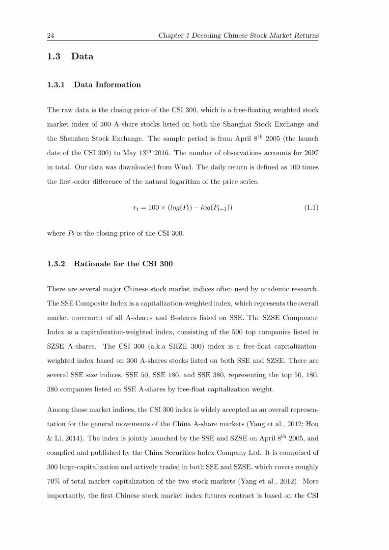
The raw data is the closing price of the CSI 300, which is a free-floating weighted stock
market index of 300 A-share stocks listed on both the Shanghai Stock Exchange and
the Shenzhen Stock Exchange. The sample period is from April 8th 2005 (the launch
date of the CSI 300) to May 13th 2016. The number of observations accounts for 2697
in total. Our data was downloaded from Wind. The daily return is defined as 100 times
the first-order difference of the natural logarithm of the price series.
rt = 100× (log(Pt)− log(Pt−1)) (1.1)
where Pt is the closing price of the CSI 300.
1.3.2 Rationale for the CSI 300
There are several major Chinese stock market indices often used by academic research.
The SSE Composite Index is a capitalization-weighted index, which represents the overall
market movement of all A-shares and B-shares listed on SSE. The SZSE Component
Index is a capitalization-weighted index, consisting of the 500 top companies listed in
SZSE A-shares. The CSI 300 (a.k.a SHZE 300) index is a free-float capitalization-
weighted index based on 300 A-shares stocks listed on both SSE and SZSE. There are
several SSE size indices, SSE 50, SSE 180, and SSE 380, representing the top 50, 180,
380 companies listed on SSE A-shares by free-float capitalization weight.
Among those market indices, the CSI 300 index is widely accepted as an overall represen-
tation for the general movements of the China A-share markets (Yang et al., 2012; Hou
& Li, 2014). The index is jointly launched by the SSE and SZSE on April 8th 2005, and
complied and published by the China Securities Index Company Ltd. It is comprised of
300 large-capitalization and actively traded in both SSE and SZSE, which covers roughly
70% of total market capitalization of the two stock markets (Yang et al., 2012). More
importantly, the first Chinese stock market index futures contract is based on the CSI
Chapter 1 Decoding Chinese Stock Market Returns 25
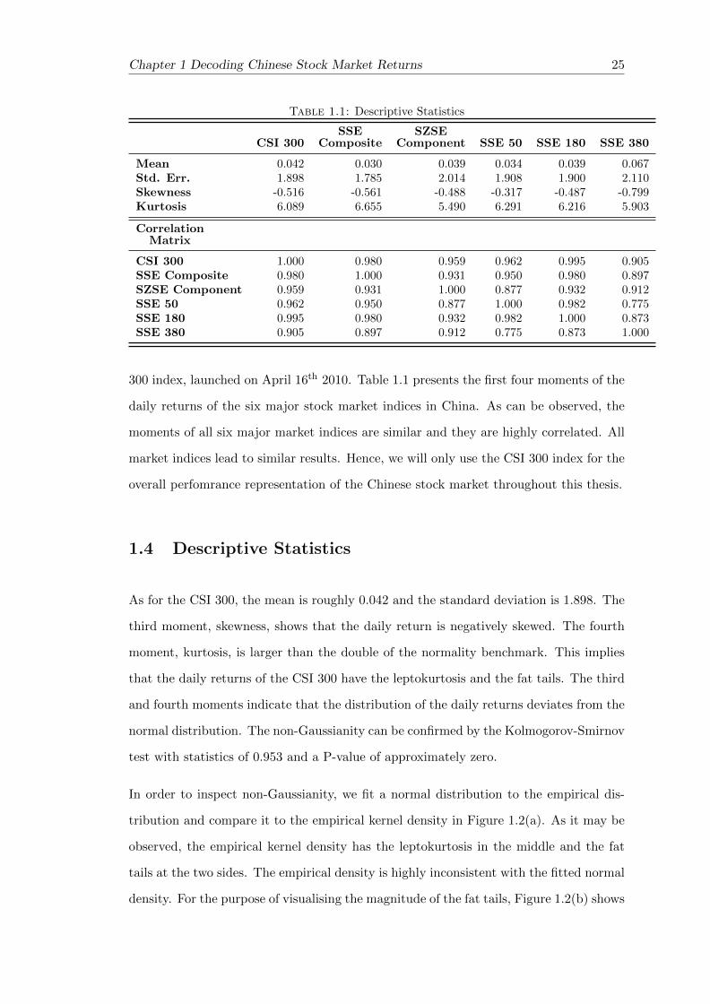
Table 1.1: Descriptive Statistics
CSI 300SSE
CompositeSZSE
Component SSE 50 SSE 180 SSE 380
Mean 0.042 0.030 0.039 0.034 0.039 0.067Std. Err. 1.898 1.785 2.014 1.908 1.900 2.110Skewness -0.516 -0.561 -0.488 -0.317 -0.487 -0.799Kurtosis 6.089 6.655 5.490 6.291 6.216 5.903
CorrelationMatrix
CSI 300 1.000 0.980 0.959 0.962 0.995 0.905SSE Composite 0.980 1.000 0.931 0.950 0.980 0.897SZSE Component 0.959 0.931 1.000 0.877 0.932 0.912SSE 50 0.962 0.950 0.877 1.000 0.982 0.775SSE 180 0.995 0.980 0.932 0.982 1.000 0.873SSE 380 0.905 0.897 0.912 0.775 0.873 1.000
300 index, launched on April 16th 2010. Table 1.1 presents the first four moments of the
daily returns of the six major stock market indices in China. As can be observed, the
moments of all six major market indices are similar and they are highly correlated. All
market indices lead to similar results. Hence, we will only use the CSI 300 index for the
overall perfomrance representation of the Chinese stock market throughout this thesis.
1.4 Descriptive Statistics
As for the CSI 300, the mean is roughly 0.042 and the standard deviation is 1.898. The
third moment, skewness, shows that the daily return is negatively skewed. The fourth
moment, kurtosis, is larger than the double of the normality benchmark. This implies
that the daily returns of the CSI 300 have the leptokurtosis and the fat tails. The third
and fourth moments indicate that the distribution of the daily returns deviates from the
normal distribution. The non-Gaussianity can be confirmed by the Kolmogorov-Smirnov
test with statistics of 0.953 and a P-value of approximately zero.
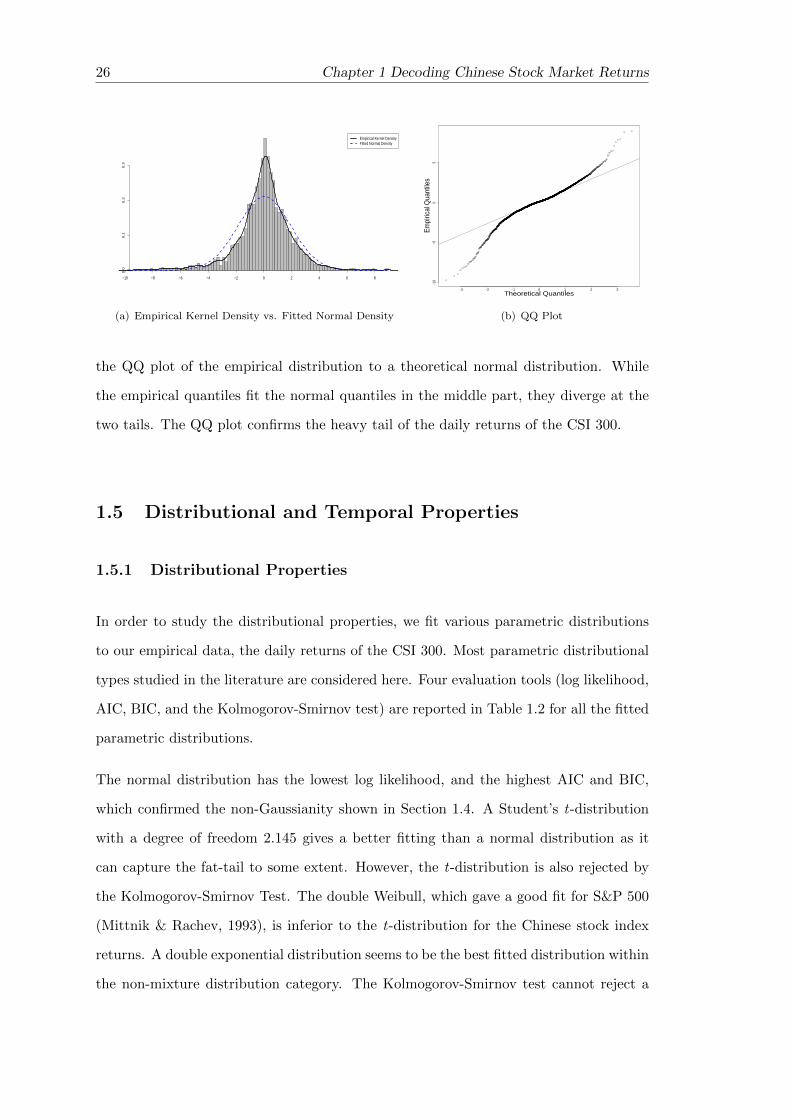
In order to inspect non-Gaussianity, we fit a normal distribution to the empirical dis-
tribution and compare it to the empirical kernel density in Figure 1.2(a). As it may be
observed, the empirical kernel density has the leptokurtosis in the middle and the fat
tails at the two sides. The empirical density is highly inconsistent with the fitted normal
density. For the purpose of visualising the magnitude of the fat tails, Figure 1.2(b) shows
26 Chapter 1 Decoding Chinese Stock Market Returns
−10 −8 −6 −4 −2 0 2 4 6 8
0.0
0.1
0.2
0.3
Empirical Kernel DensityFitted Normal Density
(a) Empirical Kernel Density vs. Fitted Normal Density
−3 −2 −1 0 1 2 3
−10
−50
5
Theoretical Quantiles
Empi
rical
Qua
ntile
s
(b) QQ Plot
the QQ plot of the empirical distribution to a theoretical normal distribution. While
the empirical quantiles fit the normal quantiles in the middle part, they diverge at the
two tails. The QQ plot confirms the heavy tail of the daily returns of the CSI 300.
1.5 Distributional and Temporal Properties
1.5.1 Distributional Properties
In order to study the distributional properties, we fit various parametric distributions
to our empirical data, the daily returns of the CSI 300. Most parametric distributional
types studied in the literature are considered here. Four evaluation tools (log likelihood,
AIC, BIC, and the Kolmogorov-Smirnov test) are reported in Table 1.2 for all the fitted
parametric distributions.
The normal distribution has the lowest log likelihood, and the highest AIC and BIC,
which confirmed the non-Gaussianity shown in Section 1.4. A Student’s t-distribution
with a degree of freedom 2.145 gives a better fitting than a normal distribution as it
can capture the fat-tail to some extent. However, the t-distribution is also rejected by
the Kolmogorov-Smirnov Test. The double Weibull, which gave a good fit for S&P 500
(Mittnik & Rachev, 1993), is inferior to the t-distribution for the Chinese stock index
returns. A double exponential distribution seems to be the best fitted distribution within
the non-mixture distribution category. The Kolmogorov-Smirnov test cannot reject a

Chapter 1 Decoding Chinese Stock Market Returns 27
double exponential distribution with a P-value of 79.83%. A symmetric hyperbolic
distribution is rejected by the Kolmogorov-Smirnov test at the 5% significance level.
If mixture distributions are considered, the Gaussian mixture distribution with two
components (Gaussian mixture (2)) is better than the double exponential distribution
with a higher log likelihood, lower AIC and BIC, and a Kolmogorov-Smirnov test P-
value of 86.20%. With an additional component, a Gaussian mixture distribution with
three components (Gaussian mixture (3)) produces a higher log likelihood. It may be
argued that the increase in likelihood comes from over-fitting by introducing more pa-
rameters. However, the AIC and BIC of Gaussian mixture (3) are lower than those of
Gaussian mixture (2). Since the AIC and BIC penalise the additional number of pa-
rameters, this suggests that Gaussian mixture (3) is superior to Gaussian mixture (2)
for Chinese stock index returns. Furthermore, a Kolmogorov-Smirnov test cannot reject
Gaussian mixture (3) at the 5% level.
The study of the fitting of various parametric distributions suggests that Gaussian mixture (3)
is a good candidate to capture the distributional properties of Chinese stock index re-
turns, which provides an intuitive foundation for using the three-state HSMM in this
paper.
1.5.2 Temporal Properties
“Long-memory”
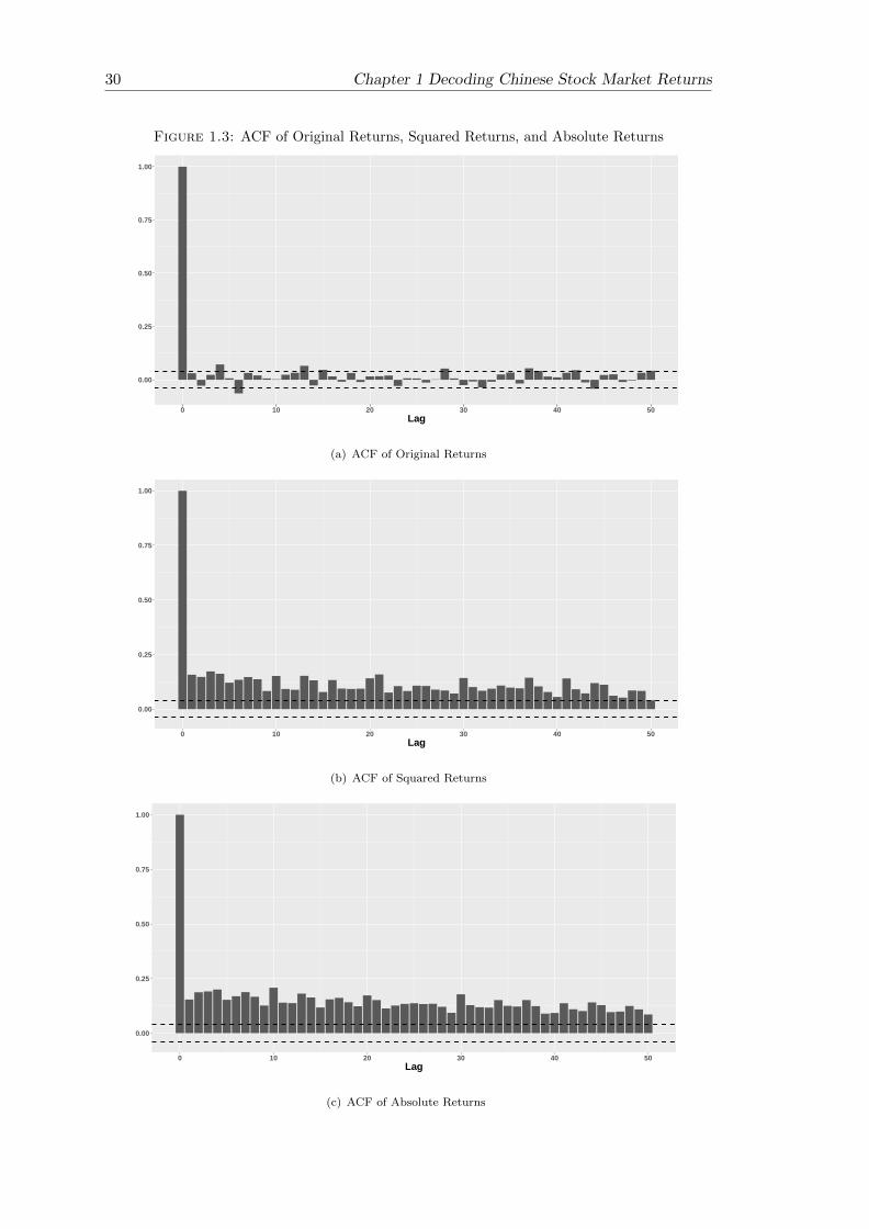
As can be seen in Figure 1.4(a), the autocorrelation functions are insignificant 1 for most
lags with a small number of exceptions. Thus, daily returns are uncorrelated. Figure
1.4(b) and Figure 1.4(c) show that the autocorrelation functions of both squared returns
and absolute returns are significant for all lags and decay slowly. This slowly decaying
autocorrelation is referred to as the “long-memory” in the literature. Both squared
returns and absolute returns are two types of volatility measure. The reason behind
the “long-memory” could be volatility clustering, which results from the fact that the
1The 95% confidence band for the autocorrelation function is calculated by ±1.96/√N , where N is
the sample size.

28 Chapter 1 Decoding Chinese Stock Market Returns
Table1.2:
Var
iou
sP
aram
etri
cD
istr
ibu
tion
Fit
tin
gs
TypeofDistribution
Fitte
dPara
mete
rsLogLikelihood
AIC
BIC
Kolm
ogoro
v-S
mirnov
Test
(P-value)
Norm
al
mea
nsd
-5554.0
54
11112.1
10
11123.9
10
0.0
0%
0.0
42
1.8
97
Stu
dent’s
tdf
-5396.7
09
10795.4
20
10801.3
20
0.0
0%
2.1
45
Double
Weibull
alp
ha
-5446.2
49
10894.5
00
10900.4
00
0.0
0%
-0.9
11
Double
Exponential
loca
tion
scale
-5339.2
19
10682.4
40
10694.2
40
79.8
3%
0.1
11
1.3
32
Symmetric
Hyperb
olic
loca
tion
scale
-5366.6
61
10737.3
20
10749.1
20
4.7
0%
0.1
01
1.8
02
Gaussian
Mixtu
re(2
)
Com
ponen
t1
-5350.6
99
10713.4
00
10748.8
00
86.2
0%
mea
nsd
wei
ght
-0.2
32
2.8
61
33.8
6%
Com
ponen
t2
mea
nsd
wei
ght
0.1
82
1.0
93
66.1
4%
Gaussian
Mixtu
re(3
)
Com
ponen
t1
-5328.9
92
10675.9
80
10729.0
80
12.2
0%
mea
nsd
wei
ght
-0.7
04
3.1
94
20.0
1%
Com
ponen
t2
mea
nsd
wei
ght
0.0
29
0.6
10
23.9
0%
Com
ponen
t3
mea
nsd
wei
ght
0.3
13
1.5
32
56.0
8%
Note
:W
euse
aone-parameter
doubleW
eibu
lldistributionF
(x)
=exp(−
(−x
)−α
)1x6
0+
1x>
0thesameasCont(2001).
Chapter 1 Decoding Chinese Stock Market Returns 29
volatility of the past returns will affect the volatility of future returns for a considerably
long period of time.
The temporal property of “long-memory” implies that there is some time dependence for
the squared/absolute returns. This time dependence is very persistent for the volatility
of returns. The GARCH-family models and the stochastic volatility models are usually
used to capture volatility clustering. A Markov chain or semi-Markov chain is also
capable of modelling volatility clustering in a discrete way. The advantage of a Markov
chain or semi-Markov chain is that they can be associated with various distributions.
Hence, the study of temporal properties gives us another incentive to use our three-state
HSMM.
Taylor Effect
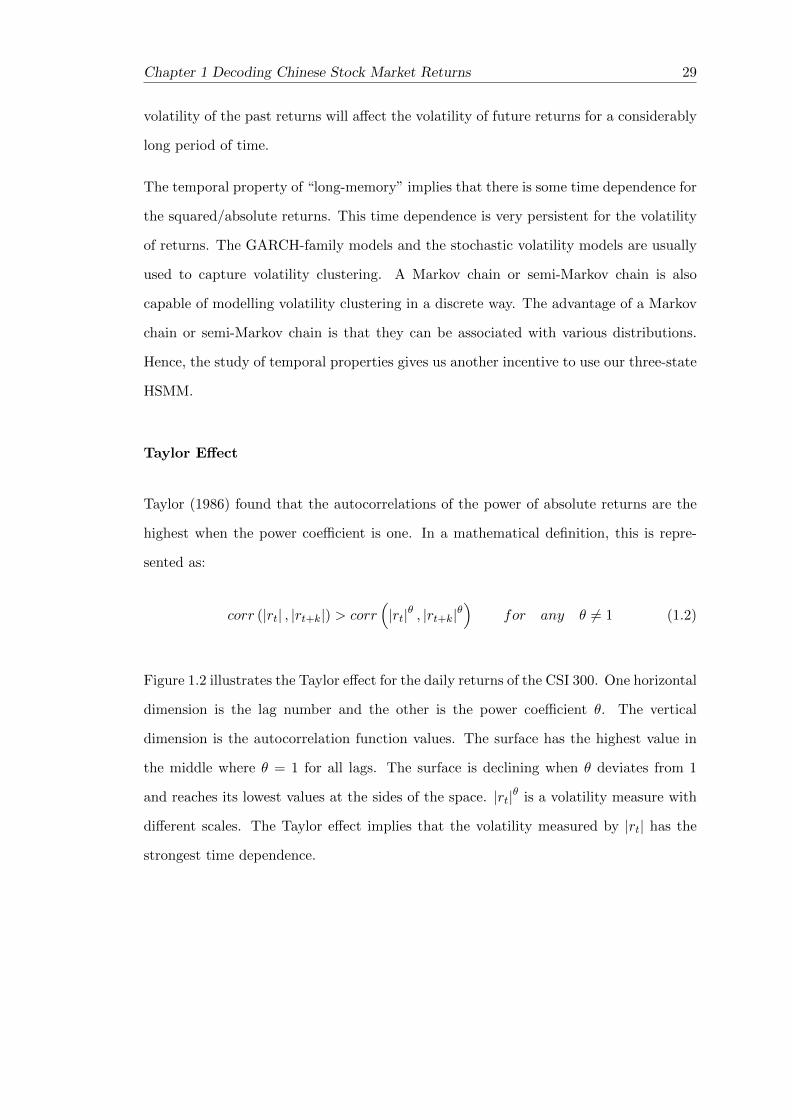
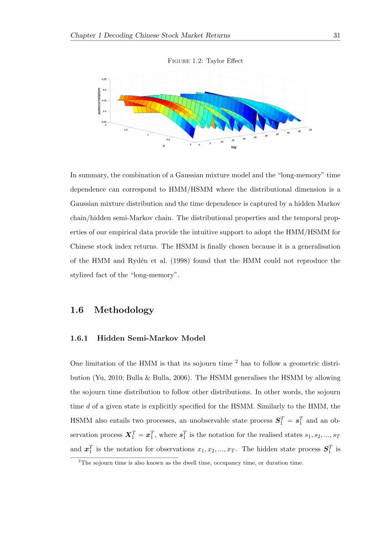
Taylor (1986) found that the autocorrelations of the power of absolute returns are the
highest when the power coefficient is one. In a mathematical definition, this is repre-
sented as:
corr (|rt| , |rt+k|) > corr(|rt|θ , |rt+k|θ
)for any θ 6= 1 (1.2)
Figure 1.2 illustrates the Taylor effect for the daily returns of the CSI 300. One horizontal
dimension is the lag number and the other is the power coefficient θ. The vertical
dimension is the autocorrelation function values. The surface has the highest value in
the middle where θ = 1 for all lags. The surface is declining when θ deviates from 1
and reaches its lowest values at the sides of the space. |rt|θ is a volatility measure with
different scales. The Taylor effect implies that the volatility measured by |rt| has the
strongest time dependence.
30 Chapter 1 Decoding Chinese Stock Market Returns
Figure 1.3: ACF of Original Returns, Squared Returns, and Absolute Returns
0.00
0.25
0.50
0.75
1.00
0 10 20 30 40 50Lag
(a) ACF of Original Returns
0.00
0.25
0.50
0.75
1.00
0 10 20 30 40 50Lag
(b) ACF of Squared Returns
0.00
0.25
0.50
0.75
1.00
0 10 20 30 40 50Lag
(c) ACF of Absolute Returns
Chapter 1 Decoding Chinese Stock Market Returns 31
Figure 1.2: Taylor Effect
0.05
2
0.1
501.5
0.15
45
au
toco
rre
lati
on
40
0.2
351 30
lag
25
0.25
200.5 1510
50 0
In summary, the combination of a Gaussian mixture model and the “long-memory” time
dependence can correspond to HMM/HSMM where the distributional dimension is a
Gaussian mixture distribution and the time dependence is captured by a hidden Markov
chain/hidden semi-Markov chain. The distributional properties and the temporal prop-
erties of our empirical data provide the intuitive support to adopt the HMM/HSMM for
Chinese stock index returns. The HSMM is finally chosen because it is a generalisation
of the HMM and Ryden et al. (1998) found that the HMM could not reproduce the
stylized fact of the “long-memory”.
1.6 Methodology
1.6.1 Hidden Semi-Markov Model
One limitation of the HMM is that its sojourn time 2 has to follow a geometric distri-
bution (Yu, 2010; Bulla & Bulla, 2006). The HSMM generalises the HSMM by allowing
the sojourn time distribution to follow other distributions. In other words, the sojourn
time d of a given state is explicitly specified for the HSMM. Similarly to the HMM, the
HSMM also entails two processes, an unobservable state process ST1 = sT1 and an ob-
servation process XT1 = xT1 , where sT1 is the notation for the realised states s1, s2, ..., sT
and xT1 is the notation for observations x1, x2, ..., xT . The hidden state process ST1 is
2The sojourn time is also known as the dwell time, occupancy time, or duration time.
32 Chapter 1 Decoding Chinese Stock Market Returns
an unobservable semi-Markov chain with m states. The observation process XT1 is asso-
ciated with the hidden state process through component distributions 3. Equation 1.3
shows the component distribution for state i at time t.
Pi(xt) = P(xt|st = i) where i ∈ {1, 2, ...,m} (1.3)
Equation 1.4 defines the state transition probability from state i to state j.
γij = P(st+1 = j|st = i) where i 6= j, i, j ∈ {1, 2, ...,m} (1.4)
Unlike the HMM, the transition probability from one state to the same state in the
HSMM is zero, i.e. γij = 0. The sojourn time in the HSMM is controlled by the sojourn
time distribution defined in Equation 1.5.
di(u) = P(st+u+1 6= i, st+ut+1 = i|st+1 = i, st 6= i) (1.5)
where the variable u is the length of the sojourn time which can follow nonparametric
or parametric distributions. The sojourn time distribution for each state i can follow
different types of distribution or the same type of distribution but with different values
of the parameters.
The transition probability matrix (TPM) has entries for the transition probabilities γij
at row i and column j. The diagonal elements in the TPM of the HSMM are zeros.
Γ =
0 γ12 · · · γ1m
γ21 0 · · · γ2m
......
. . ....
γm1 γm2 · · · 0
(1.6)
We estimate the model using the EM algorithm (see 1.A). The most likely sequence of
the states is globally decoded by the Viterbi algorithm (see 1.B.1). Additionally, we use
local decoding to compute the conditional probabilities for each state at time t given the
3The component distribution is also known as emission distribution, conditional distribution, ormarginal distribution.

Chapter 1 Decoding Chinese Stock Market Returns 33
observation (see 1.B.2). Our implementation is based on the R package ‘hsmm’ (Bulla
& Bulla, 2013).
The number of states in our HSMM is set to three. The Gaussian mixture (3) gives a
better fit than Gaussian mixture (2) based on the likelihood and the information crite-
ria. The normal distribution is chosen to be the component distribution for our HSMM.
Other distributions could be considered, but the empirical results of the Chinese stock
index returns show that the HSMM with normal components is sufficient to explain
our data. Moreover, it is convenient to conduct various tests on a normal distribution,
like the z-test in order to examine the significance of the mean. Additionally, the nor-
mal component distribution enables us to give a straightforward interpretation for the
HSMM.
As for the sojourn time distribution, the logarithmic distribution is selected because
it can produce stable estimation results while the EM algorithm may not converge
under many other sojourn time distributions. The logarithmic distribution has only
one parameter and can avoid overfitting by introducing more parameters. The negative
Binomial distribution used by Bulla & Bulla (2006) is also a suitable candidate but it
produces similar results as the logarithmic distribution. Other sojourn time distributions
could be used, but the logarithmic distribution is sufficient for our data.
1.6.2 Definition of Market Conditions
It is inevitable to propose our own definition of market conditions for three reasons.
Firstly, there is no generally accepted definition of the market conditions. Secondly,
most definitions of the market conditions are based on the monthly data. Lastly and
mostly importantly, the current definition are mainly for two-category classification, i.e.
the bull or bear market (or up or down market). The only three-category classification
is the SUD in Fabozzi & Francis (1977), but their threshold of substantial move was
arbitrarily defined. We define the bear, sidewalk, and bull market conditions from the
perspective of the distributional features.

34 Chapter 1 Decoding Chinese Stock Market Returns
Definition 1.1. A Bear Market
• The mean of the distribution of the daily returns conditional on a bear market is signifi-
cantly less than 0.
• The frequency of the positive returns is expected to be larger than that of the negative
returns.
• Because of the above statistical properties, the price in a bear market is generally decreas-
ing.
Definition 1.2. A Sidewalk Market
• The mean of the distribution of the daily returns conditional on a sidewalk market should
be insignificantly different from 0.
• It is expected to observe a roughly equal number of positive and negative returns.
• Because of the above statistical properties, the price in a sidewalk market stays in a band
and shows a mean-reversion pattern.
Definition 1.3. A Bull Market
• The mean of the distribution of the daily returns conditional on a bull market should be
significantly larger than 0.
• The frequency of the positive returns is expected to be larger than that of the negative
returns.
• Because of the above statistical properties, the price in a bull market is generally increasing.
In straight-forward notation, the mean in each market is as follows:
µ(St) = µ1 < 0, if St = 1 (bear market)
µ(St) = µ2 ≈ 0, if St = 2 (sidewalk market)
µ(St) = µ3 < 0, if St = 3 (bull market)
Chapter 1 Decoding Chinese Stock Market Returns 35
The variance of each market can be denoted as
σ2(St) = σ21, if St = 1 (bear market)
σ2(St) = σ22, if St = 2 (sidewalk market)
σ2(St) = σ23, if St = 3 (bull market)
where we expect that the bear market should have highest variance (i.e. σ21 > σ2
2, and
σ21 > σ2
3) because it is normally the most volatile market.
1.7 Empirical Results
1.7.1 Estimation Results
Through the EM algorithm, the parameters of the HSMM are estimated, including the
parameters of the component distributions, transition probability matrix, and sojourn
time distribution. Table 1.3 presents the estimated parameters of the component dis-
tributions. Based on the estimated mean and standard deviation, it is able to compute
one-sample z-statistics in order to test the significance of the mean. The formula to
compute the z-statistics is as follows.
zi =xi
σi/√ni
for i ∈ {1, 2, 3} (1.7)
where xi is the mean of state i, σi is the standard deviation of state i, and ni is the sample
size of state i. The one-sample z-test suggests that the mean of state 1 is significantly
below 0 at the 1% significance level; the mean of state 3 is significantly above 0 at the
1% significance level; whilst the mean of state 2 is insignificant from 0.
The results indicate that the time-varying distribution of the returns depends on the
hidden states, which can be interpreted as the market conditions. Specifically, state 1
corresponds to the bear market, state 2 corresponds to the sidewalk market, and state
3 corresponds to the bull market.

36 Chapter 1 Decoding Chinese Stock Market Returns
Table 1.3: Component Distribution Parameters
State 1 State 2 State 3
Mean -0.510 -0.020 0.622Std. Dev. 3.113 1.156 1.440
Sample Size 572 1430 695z-statistics 3.918∗∗∗ -0.654 11.387∗∗∗
Note: ∗p<0.1; ∗∗p<0.05; ∗∗∗p<0.01
Table 1.4 presents the empirical frequency of the positive and negative returns for the
fitted component distributions and confirms our interpretation of the three underlying
states of the HSMM. As can be seen, the frequency of the positive return of state 3 is
67.19%, while the frequency of the negative return is 32.81%. There are negative returns
in the bull market as well, but positive returns are more frequent. This statistical
evidence empowers the price in the bull market to increase. Hence, state 3 can be
regarded as a bull market according to its statistical features. Using the same logic,
state 1 has a significant negative mean and corresponds to the bear market where the
price shows a downward trend because the negative returns (52.97%) occur more often
than the positive returns (47.03%). As for state 2, the frequency of the positive and
negative returns is nearly the same at around 50%. State 2 corresponds to the sidewalk
market where the price displays a mean-reversion pattern.
Table 1.4: Frequency of Positive and Negative Returns
State 1 State 2 State 3
Positive Return Freq. 47.03% 50.49% 67.19%Negative Return Freq. 52.97% 49.51% 32.81%
Based on the estimated parameters in the component distribution, Figure 1.4 displays
the histogram of the daily returns of the CSI 300, the empirical density, and three fitted
component distribution densities. By separating the empirical distribution into three
component distributions, the HSMM is able to explain the leptokurtosis and fat tail
effects. The over-peak in the middle part of the empirical distribution mainly results
from the sidewalk market, whereas the bear market plays a vital role in the fat tails.
The standard deviation of the bear market is 3.113, which is much higher than for the
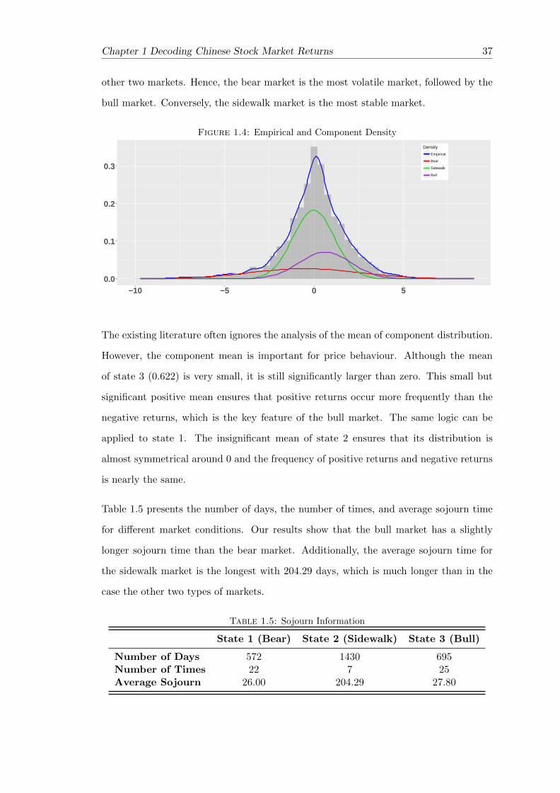
Chapter 1 Decoding Chinese Stock Market Returns 37
other two markets. Hence, the bear market is the most volatile market, followed by the
bull market. Conversely, the sidewalk market is the most stable market.
Figure 1.4: Empirical and Component Density
0.0
0.1
0.2
0.3
−10 −5 0 5
Density
Empirical
Bear
Sidewalk
Bull
The existing literature often ignores the analysis of the mean of component distribution.
However, the component mean is important for price behaviour. Although the mean
of state 3 (0.622) is very small, it is still significantly larger than zero. This small but
significant positive mean ensures that positive returns occur more frequently than the
negative returns, which is the key feature of the bull market. The same logic can be
applied to state 1. The insignificant mean of state 2 ensures that its distribution is
almost symmetrical around 0 and the frequency of positive returns and negative returns
is nearly the same.
Table 1.5 presents the number of days, the number of times, and average sojourn time
for different market conditions. Our results show that the bull market has a slightly
longer sojourn time than the bear market. Additionally, the average sojourn time for
the sidewalk market is the longest with 204.29 days, which is much longer than in the
case the other two types of markets.
Table 1.5: Sojourn Information
State 1 (Bear) State 2 (Sidewalk) State 3 (Bull)
Number of Days 572 1430 695Number of Times 22 7 25Average Sojourn 26.00 204.29 27.80

38 Chapter 1 Decoding Chinese Stock Market Returns
Table 1.6 gives the estimated transition probability matrix (TPM) of the HSMM for
the CSI 300 returns. The sojourn time of the HSMM is controlled by the sojourn time
distribution rather than by the diagonal entries in the TPM. Hence, the diagonal entries
are all zeros for the HSMM. There are a few interesting economic implications that can
be drawn from the TPM.
Table 1.6: Transition Probability Matrix
From\ To State 1 (Bear) State 2 (Sidewalk) State 3 (Bull)
State 1 (Bear) 0 0.02% 99.98%State 2 (Sidewalk) 49.56% 0 50.44%State 3 (Bull) 74.08% 25.92% 0
• After a bear market, it is highly likely (99.98%) that a bull market will follow. This
situation often occurs at the end of a crisis when the market starts to recover.
• A bear market and a bull market have equal possibility (around 50%) to occur after
a sidewalk market. In other words, it is unclear whether a bull or bear market will
follow after the price fluctuates within a certain range for a long period.
• At the end of a bull market, the market has a high probability (74.08%) to be bear
and a low probability (25.92%) to be sidewalk. These circumstances usually ensue
after a bubble burst, such as the financial crisis in 2008.
1.7.2 Decoding Results
The global decoding is conducted by the Viterbi algorithm. Figure 1.5 shows the global
decoding states with reference to the CSI 300 original series, while Figure 1.6 is correlated
with the daily returns of the CSI 300. The purple background represents the bull market,
the red background denotes the bear market, and the green background stands for the
sidewalk market. We review the evolution of the transition between the different market
conditions for the Chinese stock market in our sample period.
• At the beginning of our sample period (April 8th 2005), the Chinese stock market
was in a sidewalk market and lasted for about one year until April 27th 2006.

Chapter 1 Decoding Chinese Stock Market Returns 39
After a short period of bull (April 28th 2006 to July 14th 2006), the market became
sidewalk again and lasted for approximately 4 months (July 17th 2006 to November
13th 2006).
• At the end of 2006, the CSI 300 started to climb and reached its historically high
peak at 5877.20 on October 10th 2007. One possible reason of the boom in 2007 is
the split-share structure reform, which aimed to convert all non-tradable shares to
tradable shares. The implementation of the reform took about roughly two years
from 2005 to 2007. Due to the conversion from non-tradable shares to tradable
shares, the reform had provided substantial liquidity to the market, and it is highly
likely to be one of reason for the very promising market during that period.
• Interestingly, it is common to believe that the year 2007 is a “pure” bull market,
but our decoding results show that this period was not purely bull, but was in
fact mixed with some periods of the bear market. The mixture of the bull and
bear market can be explained by the disposition effect in the behavioural finance,
which is the phenomena that investors tend to sell assets that have gained profit
and hold assets that have lost value. In other words, investors used to cash in to
achieve capital gain following increase in stock prices and this will lead to price
reversals.
• After the financial crisis (March 12th 2007), the market went into a “pure” bear
market and the CSI 300 dropped from its peak to the bottom of 1627.76 on Novem-
ber 4th 2008, which is the largest drop in the history of the Chinese stock market.
After the market collapsed, it started to be bull and recover.
• Afterwards, the Chinese stock market experienced some periods of bear, sidewalk,
and bull alternatively. It went into a remarkably long period of sidewalk from
November 19th 2011 to November 20th 2014. During that period, the CSI 300
stayed in the range of 2000 to 3500 and displayed a mean-reversion pattern.
• From December 11th 2014, the Chinese stock market became bull and rocketed
from 3183.01 to 5335.12 on June 12th 2015, which represented an astonishing
increase of 67.61%. From the technical analysis perspective, there was a breakout

40 Chapter 1 Decoding Chinese Stock Market Returns
through the resistance line at the end of 2014, after several years of sidewalk
market. From the fundamental analysis perspective, one of the reason for this
boom was the substantial liquidity provided from the other source financing. After
this bull market, the Chinese stock market abruptly transited into a bear market.
The CSI 300 shrank to 3025.70 on August 26th 2015, which was a dramatic 43.29%
decrease. The reason of this dramatical drop in the market was highly likely to be
related to the regulations and restrictions on other source financing imposed by
CRSC in July 2015. The detail of the other source financing will be discussed in
Chapter 2.
• From September 18th 2015 to December 25th 2015, the Chinese stock market was
a bull market over the course of three months. Afterwards, a short bear market
and a short bull market occurred, followed by a sidewalk market.
The local decoding (Figure 1.7) offers a more detailed probability of each state along
with time in the sample period. The local decoding results confirm our understanding
on the transition of the market conditions of the Chinese stock market. Before 2007,
state 2 remained at a high level of probability. During 2007 and 2008, state 1 and state
3 alternatively reached high probabilities. After the financial crisis, state 1 remained at
a high probability for about one year, while the other two remained low. From 2011
to 2014, the probability of state 2 was almost 100% with a few exceptions. After 2015,
the probability of state 3 reached a relatively high level again and was followed by a
comparatively high level of state 1. State 2 has had the highest probability recently.
The local decoding results are consistent with the global decoding results.
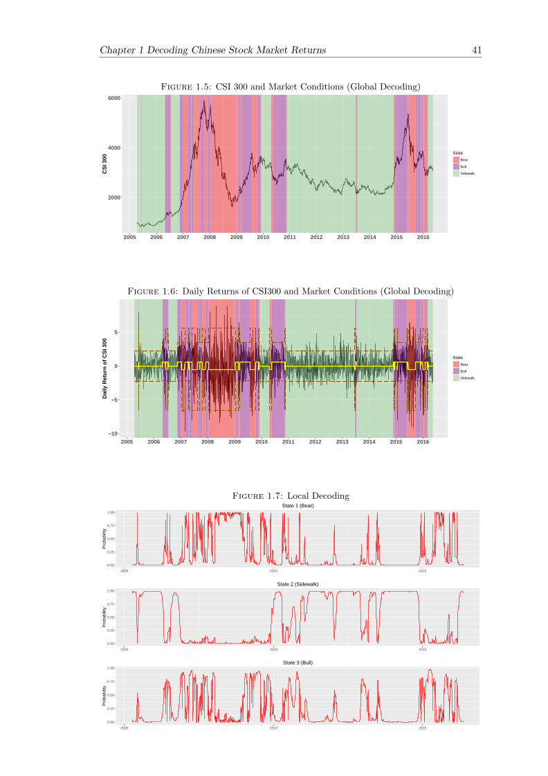
Chapter 1 Decoding Chinese Stock Market Returns 41
Figure 1.5: CSI 300 and Market Conditions (Global Decoding)
2000
4000
6000
2005 2006 2007 2008 2009 2010 2011 2012 2013 2014 2015 2016
CS
I 300
State
Bear
Bull
Sidewalk
Figure 1.6: Daily Returns of CSI300 and Market Conditions (Global Decoding)
−10
−5
0
5
2005 2006 2007 2008 2009 2010 2011 2012 2013 2014 2015 2016
Dai
ly R
etur
n of
CS
I 300
State
Bear
Bull
Sidewalk
Figure 1.7: Local Decoding
0.00
0.25
0.50
0.75
1.00
2005 2010 2015
Pro
babi
lity
State 1 (Bear)
0.00
0.25
0.50
0.75
1.00
2005 2010 2015
Pro
babi
lity
State 2 (Sidewalk)
0.00
0.25
0.50
0.75
1.00
2005 2010 2015
Pro
babi
lity
State 3 (Bull)
42 Chapter 1 Decoding Chinese Stock Market Returns
1.8 Model Evaluation and Comparison
In this section, we compare the empirical performance of our three-state HSMM with
a stochastic volatility (SV) model and a tGARCH(1,1) model in terms of three stylized
facts, namely the fat tails, the “long-memory”, and the Taylor effect.
It is worthwhile to mention the advantages and disadvantages of the HSMM and the
other alternative models. Although GARCH models are now widely used and simple
to estimate, there are three main disadvantages of these models pointed out by Nelson
(1991). Firstly, GARCH models rule out the possible situation of the negative corre-
lation between current returns and future returns volatility. Secondly, The parameter
restrictions of GARCH models can often be violated by empirical data. Thirdly, it is
difficult in GARCH models to interpret whether the shocks to conditional variance is
persist or not. As for our choice of the specific GARCH model, Hansen & Lunde (2005)
find no evidence that the GARCH(1,1) is inferior to other sophisticated ARCH-family
models by using DM-$exchange rate and daily IBM returns data. Additionally, the only
complication of tGARCH(1,1) from GARCH(1,1) is that the conditional distribution is
set to be the Student’s t-distribution in order to capture the fat-tail.
Allowing the volatility to be an unobserved continuous-time random process, SV models
overcome the disadvantages of GARCH models and fit more naturally to the modern
finance theories (Platanioti et al., 2005). Taylor (1994) show that SV models have simple
continuous-time analogues for option pricing. Yu (2002) show that the SV model is su-
perior to the GARCH models according to three different asymmetric loss functions and
Root Mean Square Error for the forecasting of the volatility of the New Zealand market
index. Although the evidence of superiority of SV models over GARCH models, their
empirical application has been limited because it is difficult to estimate the parameters
for SV model because the likelihood functions is hard to evaluate (Broto & Ruiz, 2004).
The most prominent advantage of the HSMM is that we can systemically find the hidden
states and infer the most likely sequence of the the hidden states. The main limitation
of the HSMM is that the empirical results can be largely changed by the model set-
ting, such as the number of states, the component distribution, and the sojourn time

Chapter 1 Decoding Chinese Stock Market Returns 43
distribution. Finding the appropriate model settings can involve many times of trial
and error. Additionally, using the Viterbi algorithm to conduct the global decoding is a
computational expensive procedure. To the best of our knowledge, there is no study on
the empirical performance comparison between SV models and HSMM.
Our comparison focuses on the aspects of reproducing stylized facts of asset returns.
The economic significance of the three stylized facts is as follows. Fat tails are related
to the Value-at-Risk, which plays a vital important role in financial risk management.
If the model cannot capture the correct left tail risk, the Value-at-Risk could be under-
estimated. In this circumstance, the investors may encounter an extra loss they do not
expect. It is found that the return itself is not autocorrelated but that the squared return
and the absolute return are autocorrelated and their ACF are slowly decaying. Note
that the squared return and the absolute return are both volatility measures. Hence,
the stylized fact of the “long-memory” is associated with volatility clustering, i.e. a
large volatility tends to be followed by a large volatility and a small volatility tends to
be followed by a small volatility. A good model should capture the persistence of the
volatility in asset returns. The Taylor effect is a famous statistical observation. Taylor
(1986) has initially found that the absolute return with power one has the highest au-
tocorrelation. The following literatures treat the reproduction of the Taylor effect as an
important benchmark (e.g. Ryden et al., 1998; Bulla & Bulla, 2006; Rogers & Zhang,
2011). If the model fails to reproduce the Taylor effect, then the data generation process
in the model could not fully represent the empirical asset return.
Additionally, we also compare our model with a two-state HSMM, a three-state HMM,
and a two-state HMM with respect to log likelihood, AIC, and BIC. This is for the
model selection purpose and confirms our choice of a three-state HSMM.

44 Chapter 1 Decoding Chinese Stock Market Returns
1.8.1 Comparison with Other Volatility Models
Following Jacquier et al. (1994) and Kim et al. (1998), the stochastic volatility model is
specified as
yt = eht/2εt (1.8)
ht = µ+ φ(ht−1 − µ) + σηt (1.9)
where yt is the demeaned log return, ht is the latent time-varying log volatility process,
µ is the mean level of the log volatility, φ is the persistence coefficient for the volatility
process, σ is the volatility of the log volatility, and εt and ηt are uncorrelated standard
normal white noise shocks.
We use the MCMC method developed by Kastner & Fruhwirth-Schnatter (2014) to
estimate the stochastic volatility model. As for the mean level µ ∈ R, we choose the
usual normal prior µ ∼ N (log(var(yt)), 1). The persistence parameter φ ∈ (−1, 1) is
equipped with the Beta prior (φ + 1)/2 ∼ B(20, 1). In terms of the volatility of the
log volatility σ ∈ R+, we choose σ2 ∈ 0.1 × χ21. For the MCMC setting, the thinning
parameter is set to be 10, the burn-in parameter is 5000, and the number of draw is
55000. Table 1.7 presents the posterior draws of the parameters. The posterior mean is
employed for the point estimation of the parameters.
The second benchmark model we consider is the tGARCH(1,1), which has the form
rt = µ+ σtεt, εt ∼ t(ν) (1.10)
σ2t = ω + α1y
2t−1 + β1σ
2t−1 (1.11)
where ω > 0, α1 > 0, β1 > 0, and α1 + β1 < 1. rt is the log return calculated in
Equation 2.1. The conditional distribution is set to be the Student’s t-distribution with
the degree of freedom ν. We use the quasi-maximum likelihood method (Bollerslev &
Wooldridge, 1992) to estimate the tGARCH(1,1) model, and the estimation results are
reported in Table 1.8.
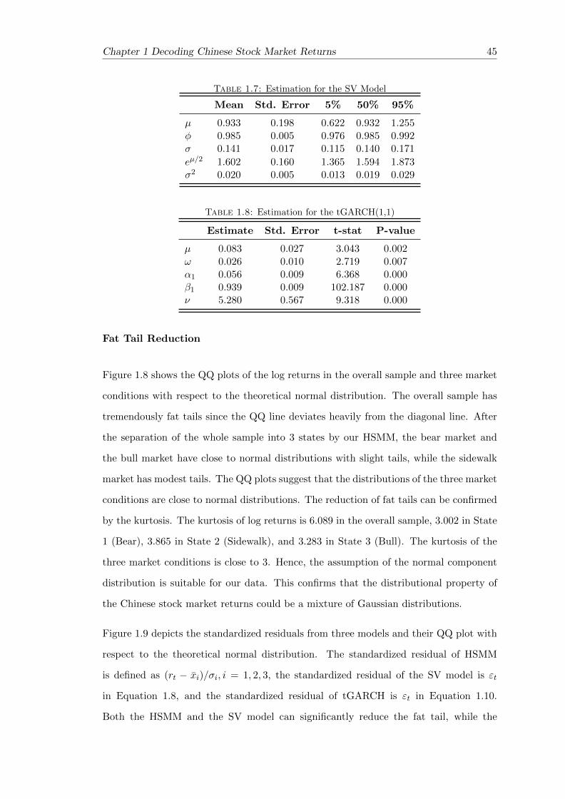
Chapter 1 Decoding Chinese Stock Market Returns 45
Table 1.7: Estimation for the SV Model
Mean Std. Error 5% 50% 95%
µ 0.933 0.198 0.622 0.932 1.255φ 0.985 0.005 0.976 0.985 0.992σ 0.141 0.017 0.115 0.140 0.171
eµ/2 1.602 0.160 1.365 1.594 1.873σ2 0.020 0.005 0.013 0.019 0.029
Table 1.8: Estimation for the tGARCH(1,1)
Estimate Std. Error t-stat P-value
µ 0.083 0.027 3.043 0.002ω 0.026 0.010 2.719 0.007α1 0.056 0.009 6.368 0.000β1 0.939 0.009 102.187 0.000ν 5.280 0.567 9.318 0.000
Fat Tail Reduction
Figure 1.8 shows the QQ plots of the log returns in the overall sample and three market
conditions with respect to the theoretical normal distribution. The overall sample has
tremendously fat tails since the QQ line deviates heavily from the diagonal line. After
the separation of the whole sample into 3 states by our HSMM, the bear market and
the bull market have close to normal distributions with slight tails, while the sidewalk
market has modest tails. The QQ plots suggest that the distributions of the three market
conditions are close to normal distributions. The reduction of fat tails can be confirmed
by the kurtosis. The kurtosis of log returns is 6.089 in the overall sample, 3.002 in State
1 (Bear), 3.865 in State 2 (Sidewalk), and 3.283 in State 3 (Bull). The kurtosis of the
three market conditions is close to 3. Hence, the assumption of the normal component
distribution is suitable for our data. This confirms that the distributional property of
the Chinese stock market returns could be a mixture of Gaussian distributions.
Figure 1.9 depicts the standardized residuals from three models and their QQ plot with
respect to the theoretical normal distribution. The standardized residual of HSMM
is defined as (rt − xi)/σi, i = 1, 2, 3, the standardized residual of the SV model is εt
in Equation 1.8, and the standardized residual of tGARCH is εt in Equation 1.10.
Both the HSMM and the SV model can significantly reduce the fat tail, while the
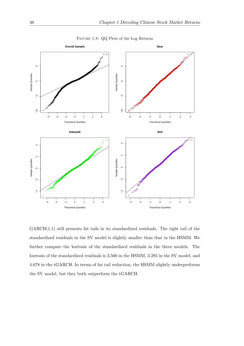
46 Chapter 1 Decoding Chinese Stock Market Returns
Figure 1.8: QQ Plots of the Log Returns
−3 −2 −1 0 1 2 3
−10
−5
05
Overall Sample
Theoretical Quantiles
Sam
ple
Qua
ntile
s
−3 −2 −1 0 1 2 3
−10
−5
05
Bear
Theoretical Quantiles
Sam
ple
Qua
ntile
s
−3 −2 −1 0 1 2 3
−4
−2
02
4
Sidewalk
Theoretical Quantiles
Sam
ple
Qua
ntile
s
−3 −2 −1 0 1 2 3
−4
−2
02
4
Bull
Theoretical Quantiles
Sam
ple
Qua
ntile
s
GARCH(1,1) still presents fat tails in its standardized residuals. The right tail of the
standardized residuals in the SV model is slightly smaller than that in the HSMM. We
further compare the kurtosis of the standardized residuals in the three models. The
kurtosis of the standardized residuals is 3.560 in the HSMM, 3.285 in the SV model, and
4.678 in the tGARCH. In terms of fat tail reduction, the HSMM slightly underperforms
the SV model, but they both outperform the tGARCH.
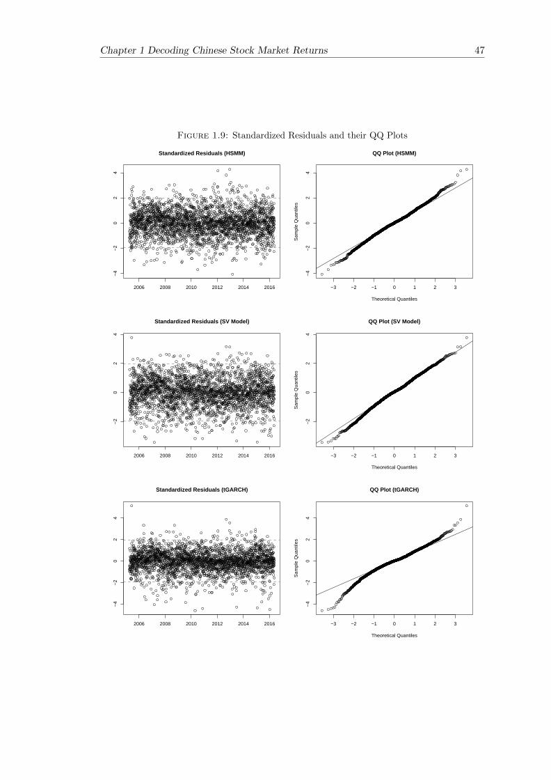
Chapter 1 Decoding Chinese Stock Market Returns 47
Figure 1.9: Standardized Residuals and their QQ Plots
2006 2008 2010 2012 2014 2016
−4
−2
02
4
Standardized Residuals (HSMM)
−3 −2 −1 0 1 2 3
−4
−2
02
4
QQ Plot (HSMM)
Theoretical QuantilesS
ampl
e Q
uant
iles
2006 2008 2010 2012 2014 2016
−2
02
4
Standardized Residuals (SV Model)
−3 −2 −1 0 1 2 3
−2
02
4
QQ Plot (SV Model)
Theoretical Quantiles
Sam
ple
Qua
ntile
s
2006 2008 2010 2012 2014 2016
−4
−2
02
4
Standardized Residuals (tGARCH)
−3 −2 −1 0 1 2 3
−4
−2
02
4
QQ Plot (tGARCH)
Theoretical Quantiles
Sam
ple
Qua
ntile
s
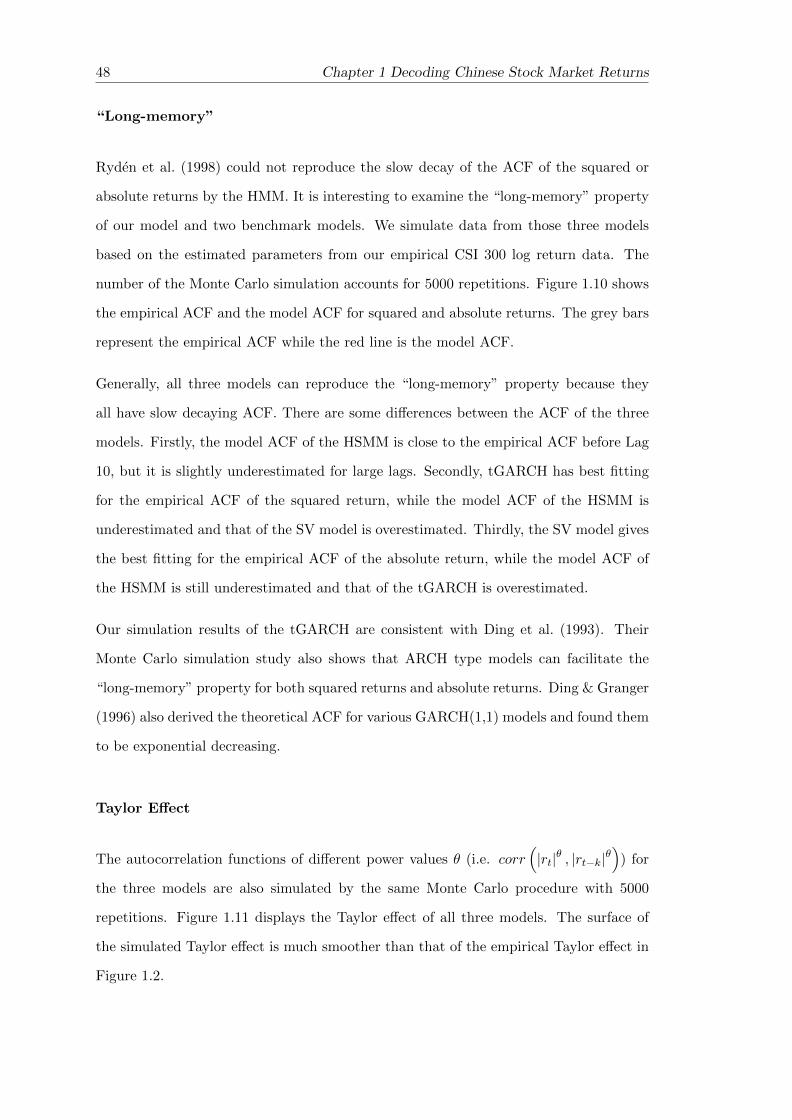
48 Chapter 1 Decoding Chinese Stock Market Returns
“Long-memory”
Ryden et al. (1998) could not reproduce the slow decay of the ACF of the squared or
absolute returns by the HMM. It is interesting to examine the “long-memory” property
of our model and two benchmark models. We simulate data from those three models
based on the estimated parameters from our empirical CSI 300 log return data. The
number of the Monte Carlo simulation accounts for 5000 repetitions. Figure 1.10 shows
the empirical ACF and the model ACF for squared and absolute returns. The grey bars
represent the empirical ACF while the red line is the model ACF.
Generally, all three models can reproduce the “long-memory” property because they
all have slow decaying ACF. There are some differences between the ACF of the three
models. Firstly, the model ACF of the HSMM is close to the empirical ACF before Lag
10, but it is slightly underestimated for large lags. Secondly, tGARCH has best fitting
for the empirical ACF of the squared return, while the model ACF of the HSMM is
underestimated and that of the SV model is overestimated. Thirdly, the SV model gives
the best fitting for the empirical ACF of the absolute return, while the model ACF of
the HSMM is still underestimated and that of the tGARCH is overestimated.
Our simulation results of the tGARCH are consistent with Ding et al. (1993). Their
Monte Carlo simulation study also shows that ARCH type models can facilitate the
“long-memory” property for both squared returns and absolute returns. Ding & Granger
(1996) also derived the theoretical ACF for various GARCH(1,1) models and found them
to be exponential decreasing.
Taylor Effect
The autocorrelation functions of different power values θ (i.e. corr(|rt|θ , |rt−k|θ
)) for
the three models are also simulated by the same Monte Carlo procedure with 5000
repetitions. Figure 1.11 displays the Taylor effect of all three models. The surface of
the simulated Taylor effect is much smoother than that of the empirical Taylor effect in
Figure 1.2.
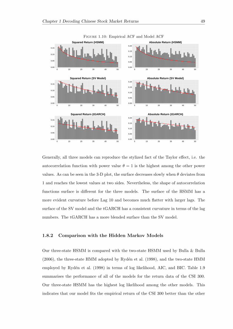
Chapter 1 Decoding Chinese Stock Market Returns 49
Figure 1.10: Empirical ACF and Model ACF
0.00
0.05
0.10
0.15
0 10 20 30 40 50
Squared Return (HSMM)
0.00
0.05
0.10
0.15
0.20
0 10 20 30 40 50
Absolute Return (HSMM)
0.00
0.05
0.10
0.15
0 10 20 30 40 50
Squared Return (SV Model)
0.00
0.05
0.10
0.15
0.20
0 10 20 30 40 50
Absolute Return (SV Model)
0.00
0.05
0.10
0.15
0 10 20 30 40 50
Squared Return (tGARCH)
0.00
0.05
0.10
0.15
0.20
0 10 20 30 40 50
Absolute Return (tGARCH)
Generally, all three models can reproduce the stylized fact of the Taylor effect, i.e. the
autocorrelation function with power value θ = 1 is the highest among the other power
values. As can be seen in the 3-D plot, the surface decreases slowly when θ deviates from
1 and reaches the lowest values at two sides. Nevertheless, the shape of autocorrelation
functions surface is different for the three models. The surface of the HSMM has a
more evident curvature before Lag 10 and becomes much flatter with larger lags. The
surface of the SV model and the tGARCH has a consistent curvature in terms of the lag
numbers. The tGARCH has a more blended surface than the SV model.
1.8.2 Comparison with the Hidden Markov Models
Our three-state HSMM is compared with the two-state HSMM used by Bulla & Bulla
(2006), the three-state HMM adopted by Ryden et al. (1998), and the two-state HMM
employed by Ryden et al. (1998) in terms of log likelihood, AIC, and BIC. Table 1.9
summarises the performance of all of the models for the return data of the CSI 300.
Our three-state HSMM has the highest log likelihood among the other models. This
indicates that our model fits the empirical return of the CSI 300 better than the other
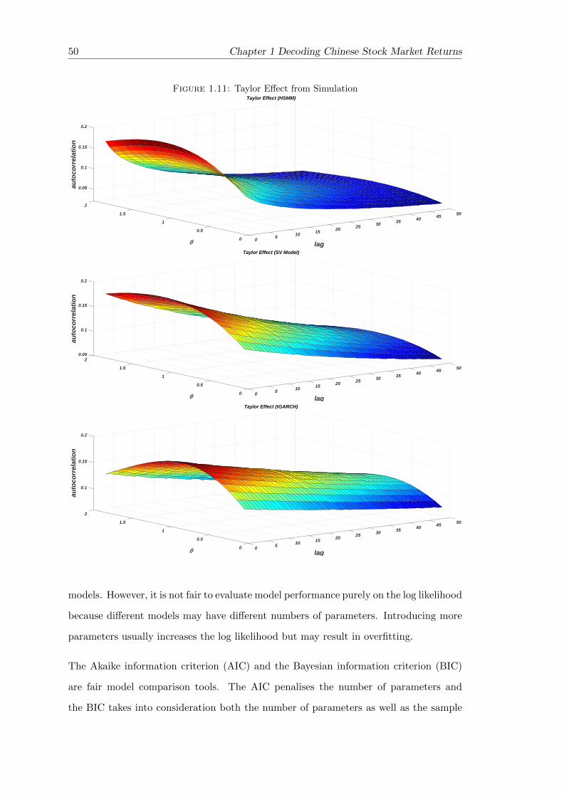
50 Chapter 1 Decoding Chinese Stock Market Returns
Figure 1.11: Taylor Effect from Simulation
2
0.05
501.5
0.1
45
au
toc
orr
ela
tio
n
40
Taylor Effect (HSMM)
0.15
351 30
lag
25
0.2
200.5 1510
50 0
0.052
0.1
501.545
au
toc
orr
ela
tio
n
40
0.15
Taylor Effect (SV Model)
351 30
lag
25
0.2
200.5 1510
50 0
2
0.1
501.545
au
toc
orr
ela
tio
n
0.15
40
Taylor Effect (tGARCH)
351 30
lag
25
0.2
200.5 1510
50 0
models. However, it is not fair to evaluate model performance purely on the log likelihood
because different models may have different numbers of parameters. Introducing more
parameters usually increases the log likelihood but may result in overfitting.
The Akaike information criterion (AIC) and the Bayesian information criterion (BIC)
are fair model comparison tools. The AIC penalises the number of parameters and
the BIC takes into consideration both the number of parameters as well as the sample
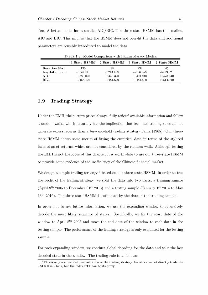
Chapter 1 Decoding Chinese Stock Market Returns 51
size. A better model has a smaller AIC/BIC. The three-state HSMM has the smallest
AIC and BIC. This implies that the HSMM does not over-fit the data and additional
parameters are sensibly introduced to model the data.
Table 1.9: Model Comparison with Hidden Markov Models
3-State HSMM 2-State HSMM 3-State HMM 2-State HMM
Iteration No. 130 18 234 45Log Likelihood -5178.911 -5213.159 -5186.953 -5229.820AIC 10385.820 10440.320 10401.910 10473.640BIC 10468.420 10481.620 10484.500 10514.940
1.9 Trading Strategy
Under the EMH, the current prices always ‘fully reflect’ available information and follow
a random walk., which naturally has the implication that technical trading rules cannot
generate excess returns than a buy-and-hold trading strategy Fama (1965). Our three-
state HSMM shows some merits of fitting the empirical data in terms of the stylized
facts of asset returns, which are not considered by the random walk. Although testing
the EMH is not the focus of this chapter, it is worthwhile to use our three-state HSMM
to provide some evidence of the inefficiency of the Chinese financial market.
We design a simple trading strategy 4 based on our three-state HSMM. In order to test
the profit of the trading strategy, we split the data into two parts, a training sample
(April 8th 2005 to December 31st 2013) and a testing sample (January 1st 2014 to May
13th 2016). The three-state HSMM is estimated by the data in the training sample.
In order not to use future information, we use the expanding window to recursively
decode the most likely sequence of states. Specifically, we fix the start date of the
window to April 8th 2005 and move the end date of the window to each date in the
testing sample. The performance of the trading strategy is only evaluated for the testing
sample.
For each expanding window, we conduct global decoding for the data and take the last
decoded state in the window. The trading rule is as follows:
4This is only a numerical demonstration of the trading strategy. Investors cannot directly trade theCSI 300 in China, but the index ETF can be its proxy.
52 Chapter 1 Decoding Chinese Stock Market Returns
• If the last decoded state is the bear market −→ Short and hold in the next trading day
• If the last decoded state is the sidewalk market −→ No position in the next trading day
• If the last decoded state is the bull market −→ Long and hold in the next trading day
Figure 1.12 shows the cumulative return of the trading strategy in the upper panel,
drawdown in the middle panel and trading signal in the lower panel. This trading
strategy is profitable with an annualised return of 37.59% and a Sharpe ratio of 1.14
5. The maximum drawdown occurred at -21.34% in January 2015. There are three
remarkable periods. The trading strategy does not have any position (trading signal:
0) before December 2014; it takes a long position (trading signal: 1) in April 2014; and
it takes a short position (trading signal: -1) from June 2015 to October 2015 and from
January 2016 to March 2016. The majority of the profit in the trading strategy comes
from the short position. During the same trading period, the buy-and-hold trading
strategy has an annual return of 13.36% and a Sharpe ratio of 0.28. Nevertheless, it
should be highlighted that the maximum drawdown of the buy-and-hold trading strategy
is -62.92%. Our simple trading strategy is superior to the buy-and-hold strategy in terms
of higher risk-adjusted return.
For the robustness test, we follow Gencay (1998) to examine the trading performance
in different out-of-sample periods. We conduct three other data split schemes and this
trading strategy still shows high profit. The robustness test results are shown in 1.C. The
robust performance of our simple trading strategy is consistent with the previous studies
shown that technical trading strategies are profitable for the stock market indices in
emerging markets (Ratner & Leal, 1999; Ito, 1999; Coutts & Cheung, 2000; Gunasekarage
& Power, 2001).
1.10 Conclusion
With the aim to decode the Chinese stock market returns, three research sub-questions
have been answered. Firstly, it is appropriate to employ a three-state HSMM to explain
5The risk free rate in China is assumed to be a constant of 4.35% according to http://www.
global-rates.com/interest-rates/central-banks/central-bank-china/pbc-interest-rate.aspx.
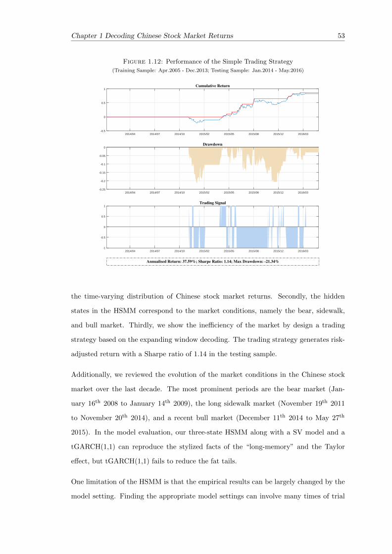
Chapter 1 Decoding Chinese Stock Market Returns 53
Figure 1.12: Performance of the Simple Trading Strategy
(Training Sample: Apr.2005 - Dec.2013; Testing Sample: Jan.2014 - May.2016)
2014/04 2014/07 2014/10 2015/02 2015/05 2015/08 2015/12 2016/03-0.5
0
0.5
1Cumulative Return
2014/04 2014/07 2014/10 2015/02 2015/05 2015/08 2015/12 2016/03-0.25
-0.2
-0.15
-0.1
-0.05
0Drawdown
2014/04 2014/07 2014/10 2015/02 2015/05 2015/08 2015/12 2016/03-1
-0.5
0
0.5
1Trading Signal
Annualised Return: 37.59%; Sharpe Ratio: 1.14; Max Drawdown: -21.34%
the time-varying distribution of Chinese stock market returns. Secondly, the hidden
states in the HSMM correspond to the market conditions, namely the bear, sidewalk,
and bull market. Thirdly, we show the inefficiency of the market by design a trading
strategy based on the expanding window decoding. The trading strategy generates risk-
adjusted return with a Sharpe ratio of 1.14 in the testing sample.
Additionally, we reviewed the evolution of the market conditions in the Chinese stock
market over the last decade. The most prominent periods are the bear market (Jan-
uary 16th 2008 to January 14th 2009), the long sidewalk market (November 19th 2011
to November 20th 2014), and a recent bull market (December 11th 2014 to May 27th
2015). In the model evaluation, our three-state HSMM along with a SV model and a
tGARCH(1,1) can reproduce the stylized facts of the “long-memory” and the Taylor
effect, but tGARCH(1,1) fails to reduce the fat tails.
One limitation of the HSMM is that the empirical results can be largely changed by the
model setting. Finding the appropriate model settings can involve many times of trial

54 Chapter 1 Decoding Chinese Stock Market Returns
and error. Future research may wish to explore the links between market conditions and
macroeconomic variables.
Appendix
1.A EM Algorithm
In this appendix, we provide technical details of the EM algorithm for the right-censored
HSMM. We adopt the right-censored HSMM because the assumption of the classical
HSMM that the last observation always coincides with the exit from a state seems to
be unrealistic for financial time series data (Bulla & Bulla, 2006). The right-censored
setting releases the assumption that the last observation is always to be the end of a
state. In other words, the last visited state will last for some time even after the last
observation. There is no immediate jump to other states after the last observation. In
the right-censored setting, the sojourn time in the last visited state is modelled by the
survivor function, which shown in Equation 1.12.
Di(u) =∑ν>u
di(u) (1.12)
Guedon (2003) provided the complete-data likelihood for the right-censored HSMM. The
complete-data likelihood function contains the observation XT1 and the state sequence
ST1 , where u − 1 is the period that the last visited state will continue after the last
observation. The last visited state will jump into other states at time T + u. The
complete-data likelihood for the right-censored HSMM is shown in Equation 1.13.
Lc(XT1 , s
T+u1 |θ) = P(XT
1 = xT1 ,ST1 = sT1 ,S
T+u−1T+1 = sT , ST+u 6= sT |θ) (1.13)
55
56 Chapter 1 Decoding Chinese Stock Market Returns
The final likelihood function is obtained by summing all possible state sequences and all
possible prolongation lengths of the last state, as indicated in Equation 1.14.
L(θ) =∑
t=S1,...,ST
∑uT+
Lc(XT1 , s
T+u1 |θ) (1.14)
where∑
t=S1,...,STrepresents the summation of all possible state sequences, and
∑uT+
represents the summation over all possible additional sojourn time after time T .
It is difficult to compute the likelihood function in Equation 1.13 because the under-
lying state sequence is unknown. It needs to consider all possibilities of the state se-
quence in order to compute the full likelihood, which is not realistic. The expectation-
maximization (EM) algorithm provides a suitable procedure to deal with the missing
data problem. The EM algorithm (Baum et al., 1970) is an iterative procedure to
increase the likelihood until it reaches the convergence criteria. The EM algorithm iter-
atively conducts the E-step and M-step. Given an initial guess of the parameter vector
θ , the E-step firstly computes the Q-function, which is the conditional expectation for
the complete-data likelihood.
• E-step
Q(θ,θ(t−1)) = E{Lc(X
T1 , s
T+u1 |θ)|XT
1 = xT1 ,θ(t−1)
}(1.15)
Based on the Q-function in Equation (12), the M-step aims to maximise the Q-
function with respect to parameter θ.
• M-step
θ(t) = arg maxθ
Q(θ,θ(t−1)) (1.16)
The parameter vector θ that maximises the Q-function in the M-step of the previous
iteration will be used in the E-step of the next iteration. Along with every iteration,
the likelihood is non-decreasing. The algorithm will stop once the convergence criterion
is satisfied. Normally, the convergence criterion is the successive change of likelihood is
less than a very small number. The EM algorithm is not guaranteed to reach the global
maxima and it might be trapped in local maxima. Hence, it is necessary to try different
Chapter 1 Decoding Chinese Stock Market Returns 57
initial values of parameter vector θ in order to check that the maximum reached is the
global maximum rather than the local maximum.
In this chapter, we focused on the economic interpretation of the HSMM rather than on
the mathematical derivation. We direct the reader to the thesis of Bulla (2006) for the
mathematical details of the EM algorithm of the HSMM. In his thesis, he decomposes the
Q-function of the HSMM into four components, which correspond to the initial proba-
bilities, transition probabilities, sojourn time, and component distributions. The E-step
is implemented by the forward-backward algorithm. His decomposition framework fa-
cilities the M-step in which the four components can be maximised individually. Bulla
shows the close-form solutions for some common distributions for the sojourn time and
component distributions, but the numerical solver could be applied if a closed solution
does not exist.
Unlike the maximum likelihood method whereby the standard errors can be directly
calculated by the Fisher information matrix (FIM), one drawback of the EM algorithm is
that the FIM is not a by-product of the algorithm. It is highly unlikely to obtain the FIM
by evaluating analytically the second-order derivatives of the marginal log-likelihood of
the HSMM. Recent numerical methods are developed to get an approximation of the
FIM (see Louis, 1982; Meng & Rubin, 1991; Jamshidian & Jennrich, 2000). However, all
these methods have limitations (Meng, 2016). There is no generally accepted method
to get diagnosis for the estimation of the HSMM by the EM algorithm. Hence, we do
not provide the diagnosis of the estimated parameters in this chapter.
1.B Decoding Technique
It is interesting to decode the most likely states in the Markov chain. There are two
decoding techniques for the HSMM, global decoding and local decoding. Global decoding
aims to determine the most likely sequence of the states given the observations, while
the local decoding computes the conditional probability of each state at times given the
observations. Normally, they produce similar but not identical decoding results.
58 Chapter 1 Decoding Chinese Stock Market Returns
1.B.1 Global Decoding
The purpose of global decoding is to find the most likely sequence of states conditional on
the observations. Mathematically speaking, global decoding intends to find a sequence
of states with the highest likelihood given the observations, which is shown in Equation
1.17.
ST1 = arg maxST1
P(ST1 |XT
1
)(1.17)
The exhaustive attack method has the computational complexity level at O(mT ). This
brute force method is not feasible for long sequence data. The Viterbi algorithm (Viterbi,
1967) was developed by utilising the Markov property of the HMM and HSMM. This is
an efficient dynamic programming algorithm and its complexity level is O(m× T ). The
Viterbi algorithm works in the following way.
arg maxST1
P(ST1 |XT
1
)= arg max
ST1
P(ST1 ,X
T1
)(1.18)
Define
µt(St) = maxSt−1
1
P(St1,Xt1) (1.19)
The recursion expression for maxP(St1,Xt1) can be derived.
maxSt−1
1
P(St1,Xt1) = max
St−11
P(Xt|St)P(St|St−1)P(St−11 ,Xt−1
1 )
= maxSt−1
{P(Xt|St)P(St|St−1) max
St−21
P(St−11 ,Xt−1
1 )
}
= maxSt−1
P(Xt|St)P(St|St−1)µt−1(St−1)
(1.20)
The recursion equation for µt(St) is as follows
µt(St) = maxSt−1
P(Xt|St)P(St|St−1)µt−1(St−1) for t = 2, ..., T (1.21)
Equation 1.21 is able to compute the most likely trajectory for each state up to time
t. At time T , the state with the highest P(ST1 ,XT1 ) is picked up and the corresponding
trajectory is the solution for the Viterbi algorithm.
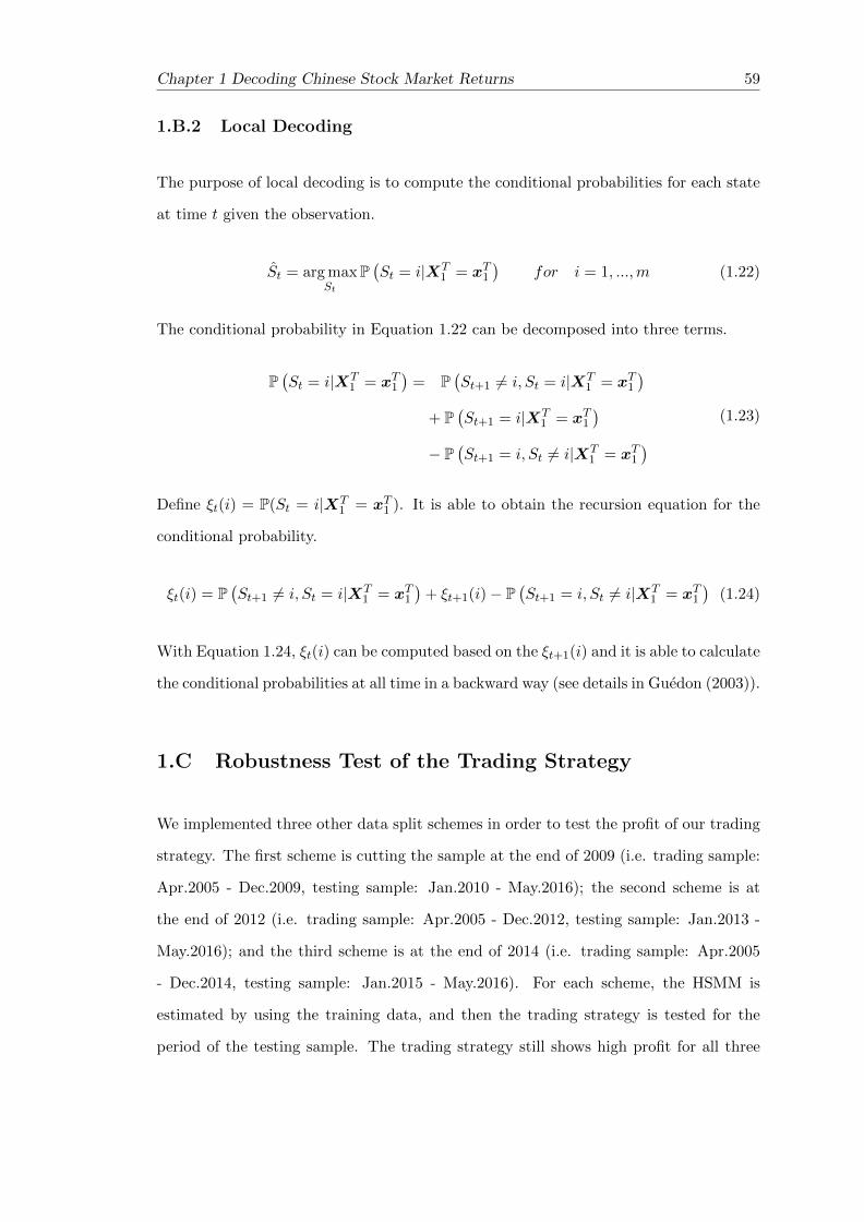
Chapter 1 Decoding Chinese Stock Market Returns 59
1.B.2 Local Decoding
The purpose of local decoding is to compute the conditional probabilities for each state
at time t given the observation.
St = arg maxSt
P(St = i|XT
1 = xT1)
for i = 1, ...,m (1.22)
The conditional probability in Equation 1.22 can be decomposed into three terms.
P(St = i|XT
1 = xT1)
= P(St+1 6= i, St = i|XT
1 = xT1)
+ P(St+1 = i|XT
1 = xT1)
− P(St+1 = i, St 6= i|XT
1 = xT1) (1.23)
Define ξt(i) = P(St = i|XT1 = xT1 ). It is able to obtain the recursion equation for the
conditional probability.
ξt(i) = P(St+1 6= i, St = i|XT
1 = xT1)
+ ξt+1(i)− P(St+1 = i, St 6= i|XT
1 = xT1)
(1.24)
With Equation 1.24, ξt(i) can be computed based on the ξt+1(i) and it is able to calculate
the conditional probabilities at all time in a backward way (see details in Guedon (2003)).
1.C Robustness Test of the Trading Strategy
We implemented three other data split schemes in order to test the profit of our trading
strategy. The first scheme is cutting the sample at the end of 2009 (i.e. trading sample:
Apr.2005 - Dec.2009, testing sample: Jan.2010 - May.2016); the second scheme is at
the end of 2012 (i.e. trading sample: Apr.2005 - Dec.2012, testing sample: Jan.2013 -
May.2016); and the third scheme is at the end of 2014 (i.e. trading sample: Apr.2005
- Dec.2014, testing sample: Jan.2015 - May.2016). For each scheme, the HSMM is
estimated by using the training data, and then the trading strategy is tested for the
period of the testing sample. The trading strategy still shows high profit for all three
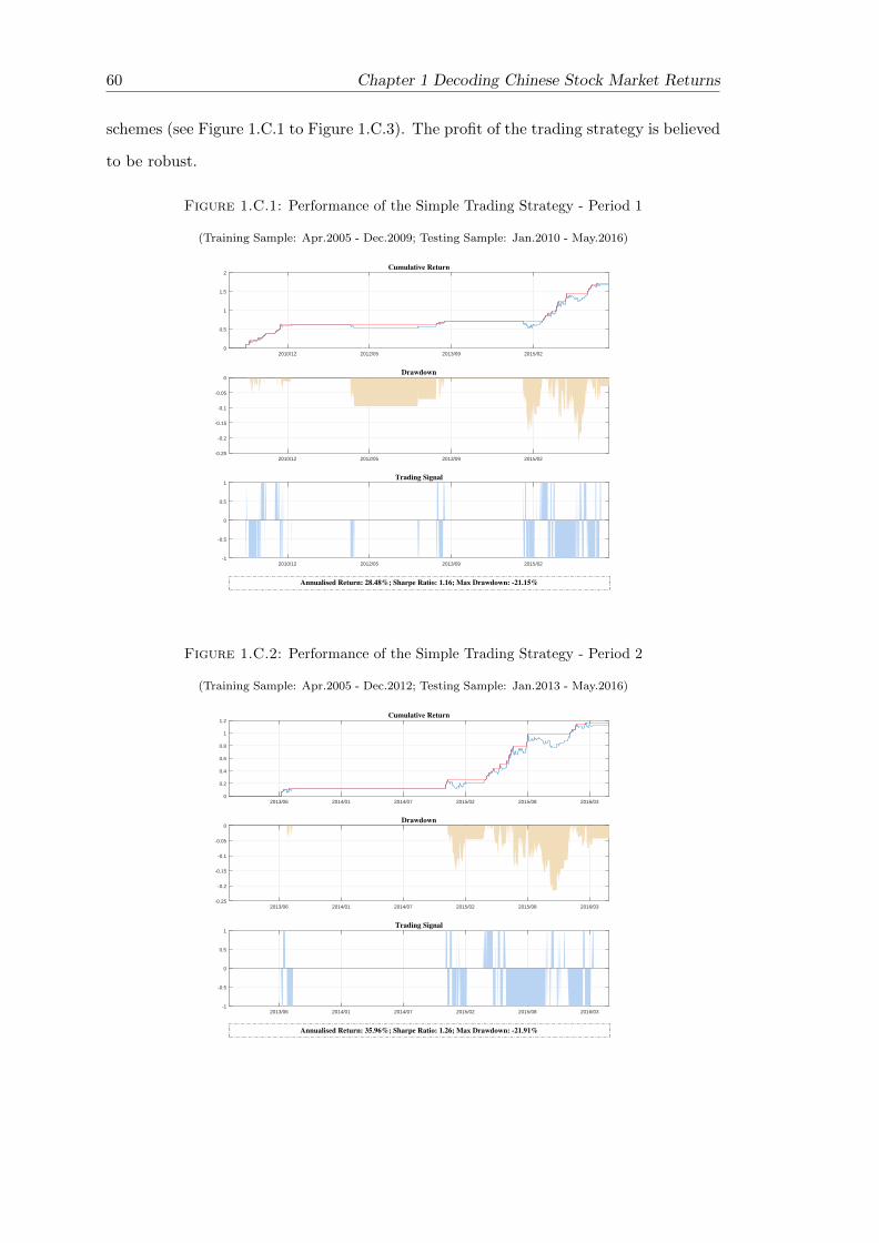
60 Chapter 1 Decoding Chinese Stock Market Returns
schemes (see Figure 1.C.1 to Figure 1.C.3). The profit of the trading strategy is believed
to be robust.
Figure 1.C.1: Performance of the Simple Trading Strategy - Period 1
(Training Sample: Apr.2005 - Dec.2009; Testing Sample: Jan.2010 - May.2016)
2010/12 2012/05 2013/09 2015/020
0.5
1
1.5
2Cumulative Return
2010/12 2012/05 2013/09 2015/02-0.25
-0.2
-0.15
-0.1
-0.05
0Drawdown
2010/12 2012/05 2013/09 2015/02-1
-0.5
0
0.5
1Trading Signal
Annualised Return: 28.48%; Sharpe Ratio: 1.16; Max Drawdown: -21.15%
Figure 1.C.2: Performance of the Simple Trading Strategy - Period 2
(Training Sample: Apr.2005 - Dec.2012; Testing Sample: Jan.2013 - May.2016)
2013/06 2014/01 2014/07 2015/02 2015/08 2016/030
0.2
0.4
0.6
0.8
1
1.2Cumulative Return
2013/06 2014/01 2014/07 2015/02 2015/08 2016/03-0.25
-0.2
-0.15
-0.1
-0.05
0Drawdown
2013/06 2014/01 2014/07 2015/02 2015/08 2016/03-1
-0.5
0
0.5
1Trading Signal
Annualised Return: 35.96%; Sharpe Ratio: 1.26; Max Drawdown: -21.91%
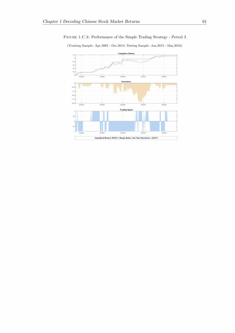
Chapter 1 Decoding Chinese Stock Market Returns 61
Figure 1.C.3: Performance of the Simple Trading Strategy - Period 3
(Training Sample: Apr.2005 - Dec.2014; Testing Sample: Jan.2015 - May.2016)
2015/02 2015/05 2015/08 2015/12 2016/030
0.2
0.4
0.6
0.8
1
1.2Cumulative Return
2015/02 2015/05 2015/08 2015/12 2016/03-0.25
-0.2
-0.15
-0.1
-0.05
0Drawdown
2015/02 2015/05 2015/08 2015/12 2016/03-1
-0.5
0
0.5
1Trading Signal
Annualised Return: 89.06%; Sharpe Ratio: 2.26; Max Drawdown: -24.43%

Chapter 2
Understanding the Chinese Stock Market:
International Comparison and Policy Implications
The definition of bear, sidewalk, and bull markets is ambiguous in existing literature.
This makes it difficult for practitioners to distinguish between different market condi-
tions. In this chapter, we employ a statistical definition of bear, sidewalk, and bull
markets, which correspond to the three states in our hidden semi-Markov model. We
employ this analysis to the daily returns of the Chinese stock market and the other seven
developed markets investigated. Using the Viterbi algorithm to globally decode the most
likely sequence of the market conditions, we systematically find the precise timing of bear,
sidewalk, and bull markets for all eight markets. Through the comparison of the estima-
tion and decoding results, many unique characteristics of the Chinese stock market are
found, such as “Crazy Bull”, “Frequent and Quick Bear”, and “No Buffer Zone”. In
China, the bull market is more volatile than in developed markets, the bear market occurs
more frequently than in developed markets, and the sidewalk market has not functioned
as a buffer zone since 2005. Lastly, the possible causes of the unique characteristics are
discussed and implications for policy-making are suggested.
63
64 Chapter 2 Understanding the Chinese Stock Market
2.1 Introduction
In the last two decades, China has made significant progress on the development of the
stock market. A number of important steps have been carried out, such as the enactment
of Qualified Foreign Institutional Investors (QFII) programme in 2002, the split-share
structure reform in 2005, and the Qualified Domestic Institutional Investors (QDII)
programme in 2006. However, the current rules and structures of the Chinese stock
market are still considerably different from those of developed stock markets. Firstly,
the Chinese stock market is relatively isolated from the international financial markets
because of very limited openness to the international investors. Secondly, the Chinese
stock market is heavily regulated and intervened by the government. Thirdly, the Chi-
nese stock market is still under development and lacks financial derivatives to manage
risk. Lastly, the majority of investors are individual investors without professional in-
vestment knowledge, who are focusing on short-term speculation, rather than long-term
investment. Lastly, the Chinese stock market is very liquid with high turnover velocity.
It is natural to raise the question how these different rules and structures reflect on the
market behaviour. Many studies have investigated the Chinese stock market. Herd-
ing behaviour, overreaction, and speculation in the Chinese stock market are well-
documented (Tan et al., 2008; Mei et al., 2009; Ni et al., 2015). However, less attention
has been to paid from the perspective of the market condition. To the best of our knowl-
edge, very limited study has identified the difference of the market conditions between
the Chinese stock market and developed markets, especially after 2005. In this chap-
ter, we are interested in investigating the unique characteristics of market conditions in
China with particular comparison to developed markets. Additionally, we discuss the
possible causes of the unique characteristics of market conditions in China and propose
several policy suggestions to help the development of the Chinese stock market.
The definition of bear, sidewalk, and bull markets is very vague in the existing literature,
making it difficult for practitioners to distinguish between stock markets in different
market conditions. We employ a statistical definition of bear, sidewalk, and bull markets,
which corresponds to the states in our three-state hidden semi-Markov model (HSMM) in

Chapter 2 Understanding the Chinese Stock Market 65
Chapter 1. We employ this analysis to the daily return of the Chinese stock market and
the other seven developed markets analysed. Using the Viterbi algorithm (Viterbi, 1967)
to globally decode the most likely sequence of the market conditions, we systematically
find the precise timing of bear, sidewalk, and bull markets for all eight markets. Through
the comparison of the estimation and decoding results, several unique characteristics of
the Chinese stock market are found, such as “Crazy Bull”, “Frequent and Quick Bear”,
and “No Buffer Zone”. “Crazy Bull” refers to the observation that the bull market has a
considerably high variance. “Frequent and Quick Bear” is the observation that the bear
market has short sojourn time and occurs very frequently. “No Buffer Zone” represents
the observation that the bull market is typically mixed with the bear market and there
is no sidewalk market between them.
Our findings are meaningful for investors and policy makers on two levels. Firstly, at the
micro-level, investors have more in-depth understanding of the Chinese stock market,
which has several prominent differences from developed markets. In China, the bull
market is more volatile, the bear market happens more frequently, and the sidewalk
market does not function as a buffer zone. All of these characteristics suggest that
investors need to carefully manage the risk of their investment and avoid speculation.
Secondly, at the macro-level, it is vital for the government to educate individual investors
and develop institutional investors, to provide more accessible risk management tools,
and to strengthen regulation on excess leverage from other source financing.
2.2 Literature Review
Many studies have investigated the Chinese stock market. Herding behaviour, overreac-
tion, and speculation in the Chinese stock market are well-documented. Tan et al. (2008)
studied heading behaviour in the Chinese stock market, both A-share and B-share. They
found that herding happens in both upside and downside market conditions. Particu-
larly, herding behaviour is stronger in upside market conditions in A-share. Investor
sentiment and its nonlinear effect on stock returns in China was studied by Ni et al.
(2015) through the panel quantile regression model. The nonlinear effect of investor

66 Chapter 2 Understanding the Chinese Stock Market
sentiment turns out to be asymmetric and reversal, which proves the occurrence of
overreaction in the Chinese stock market. Additionally, it was observed that Chinese
investors are affected by cognitive bias and speculation tendencies.
The market condition has been studied by Markov-switching techniques. Schaller &
Norden (1997) considered a two-regime model which allows the mean and/or the vari-
ance of returns to vary in different regimes for the US stock market. Nielsen et al.
(2001) found that a third regime, the speculative market, exists in some European mar-
kets. Girardin & Liu (2003) adopted a switch-in-the-mean plus switch-in-the-variance
(MSMH(3)-AR(5)) model for weekly capital gains on the Shanghai A-share market dur-
ing the period between 1995 and 2002. They also found that there are three market
conditions: a speculative market, a bull market and a bear market. They claimed that
the bull market is always a buffer zone in the transition between the other two market
conditions. It should be noted that the buffer zone defined in the context of Girardin &
Liu (2003) is the bull market, while the sidewalk market is regarded as the buffer zone
in this chapter.
The hidden Markov model (HMM) and hidden semi-Markov model (HSMM) used in
financial studies focus on the reproduction of stylized facts of daily returns. Ryden
et al. (1998) firstly adopted a two-state HMM with normal distributions (zero mean
but different variance) as the component distribution (a.k.a. marginal distribution) to
reproduce most of the stylized facts of daily returns, except for the slow decay in the
autocorrelation function of squared returns. Bulla & Bulla (2006) used a two-state
HSMM, which is a generalization of HMM, to model daily returns of 18 US sector
indexes. The stylized facts of daily returns are reproduced by HSMM, including the
long-memory in the autocorrelation function of squared returns. In Chapter 1, we used
a three-state HSMM on the daily returns of CSI 300 and showed that the stylized facts of
daily return in China also can be reproduced. The empirical results suggest that three-
state HSMM is appropriate for the CSI 300, and it is better than two-state HSMM,
three-state hidden Markov model, and two-state hidden Markov model model. In this
Chapter, we employ the same three-state HSMM as in Chapter 1 to systematically find
the precise timing of bear, sidewalk, and bull markets.

Chapter 2 Understanding the Chinese Stock Market 67
This chapter firstly propose the statistical definitions of bear, sidewalk, and bull markets.
In the empirical results part, the unique characteristics of the Chinese stock market are
identified through the comparison of estimation and decoding results with developed
markets. Finally, the possible causes of the unique characteristics are discussed and
several policy implications are suggested.
2.3 Definition of Bear, Sidewalk, and Bull
In practice, investors tend to determine market conditions arbitrarily and different con-
clusions might be drawn for the same market in the same period. In the existing aca-
demic literature, the definition of market conditions varies considerably. In one of the
early study, Fabozzi & Francis (1977) propose three ways to define market conditions.
In the first classification of Bull and Bear Markets, the rule places most months when
the market rises in the bull market (BB), but months when the market rose near the
bearish months were treated as part of the bear market. In the second classification
of Up and Down Markets (UD), months in which return was non-negative are defined
as Up months and months in which return was negative are defined as Down months.
In the third classification of Substantial Up and Down Months (SUD), there are three
categories: months when the market moved Up-substantially, months when the market
moved Down-substantially, and months when the market moved neither Up-substantially
nor Down-substantially. The threshold of substantial move was arbitrarily defined.
In the modern study, a loose definition by Chauvet & Potter (2000) proposed that market
prices generally increase (decrease) in a bull (bear) market. Edwards & Caglayan (2001)
use a simple classification that bull market months are defined as those in which the
S&P index rises by 1% or more and bear market months are defined as those in which
the S&P index falls by 1% or more. Lunde & Timmermann (2004) claim that a bull
(bear) market starts when the market price increases (decreases) a certain percentage,
say 20%, from the previous local bottom (peak). Gonzalez et al. (2006) utilized two
formal turning point methods to detect the timing of bull and bear markets. Cheng

68 Chapter 2 Understanding the Chinese Stock Market
et al. (2013) define bull (bear) markets as the periods with at least three consecutive
months of positive (negative) returns.
It is inevitable to propose our own definition of market conditions for three reasons.
Firstly, there is no generally accepted definition of the market conditions. Secondly,
most definitions of the market conditions are based on the monthly data. Lastly and
mostly importantly, the current definition are mainly for two-category classification, i.e.
the bull or bear market (or up or down market). The only three-category classification
is the SUD in Fabozzi & Francis (1977), but their threshold of substantial move was
arbitrarily defined. We define the bear, sidewalk, and bull market conditions from the
perspective of the distributional features.
Definition 2.1. A Bear Market
• The mean of the distribution of the daily returns conditional on a bear market is signifi-
cantly less than 0.
• The frequency of the positive returns is expected to be larger than that of the negative
returns.
• Because of the above statistical properties, the price in a bear market is generally decreasing.
Definition 2.2. A Sidewalk Market
• The mean of the distribution of the daily returns conditional on a sidewalk market should
be insignificantly different from 0.
• It is expected to observe a roughly equal number of positive and negative returns.
• Because of the above statistical properties, the price in a sidewalk market stays in a band
and shows a mean-reversion pattern.
Definition 2.3. A Bull Market
• The mean of the distribution of the daily returns conditional on a bull market should be
significantly larger than 0.
• The frequency of the positive returns is expected to be larger than that of the negative
returns.
• Because of the above statistical properties, the price in a bull market is generally increasing.
Chapter 2 Understanding the Chinese Stock Market 69
In straight-forward notation, the mean in each market is as follows:
µ(St) = µ1 < 0, if St = 1 (bear market)
µ(St) = µ2 ≈ 0, if St = 2 (sidewalk market)
µ(St) = µ3 < 0, if St = 3 (bull market)
The variance of each market can be denoted as
σ2(St) = σ21, if St = 1 (bear market)
σ2(St) = σ22, if St = 2 (sidewalk market)
σ2(St) = σ23, if St = 3 (bull market)
where we expect that the bear market should have highest variance (i.e. σ21 > σ2
2, and
σ21 > σ2
3) because it is normally the most volatile market.
2.4 Empirical Results
2.4.1 Data Description
We apply the three-state HSMM to analyse the daily returns of stock indexes in eight
countries, including the CSI 300 (China), S&P 500 (United States), FTSE 100 (United
Kingdom), CAC 40 (France), DAX (Germany), Nikkei 225 (Japan), STI (Singapore),
and ASX 200 (Australia). The sample period is from April 8th 2005 to February 26th
2016 1, slightly more than a decade. The reason for using this sample period is that
the start date is when the CSI 300 was first launched. Additionally, As the split-
share structure reform occurred in 2005, the behavior of Chinese stock market has a
structural change. Interested readers can refer to Girardin & Liu (2003) the research
for the Chinese stock market during 1997 to 2002. There are 2645 observations for each
index. The source of our data is Wind.
1Note that the sample period is slightly shorter than the sample period used in Chapter 1.
70 Chapter 2 Understanding the Chinese Stock Market
The daily return is defined as 100 times the first-order difference of the natural logarithm
of the price series.
rit = 100× (log(P it )− log(P it−1)) (2.1)
where P it is the closing price of the market index i at time t.
2.4.2 Component Distribution - Evidence of “Crazy Bull”
It is natural to interpret the three states in our HSMM as bear, sidewalk, and bull
according to our definition based on statistical features of return distributions. The
estimated parameters of the component distribution in HSMM for all countries are
presented in Table 2.1. The means of State 1 in all countries are less than zero and
their variances are the highest among the three states. The statistical features of State
1 are consistent with a bear market. It can be observed that the means in State 2 are
all close to zero and slightly less to zero. The variance in State 2 is much lower than in
State 1. The statistical features of State 2 meet our expectation of a sidewalk market,
in which the return distribution should have a mean close to zero, enabling the price in
the sidewalk market to fluctuate within a band. State 3 for all countries have positive
means with the smallest variance among all of the states, except for the CSI 300. The
return distribution with positive mean and small variance allows the price in the bull
market to increase steadily, which is an intrinsic feature of a bull market.
The first unique characteristic of the Crazy Bull is the abnormally high variance in
the Chinese bull market compared with other countries. The Chinese bull market has
a variance of 2.058, almost three times higher than for other countries. Japan has
the second most unstable bull market with a variance of 0.693. The bull market in
the United States and the United Kingdom are relatively more stable, as indicated by
the small variances of 0.244 and 0.297, respectively. It is reasonable to expect that
the variance is higher in the bear market for all eight countries since the abrupt price
fall during the market crash make the volatility increase. The bear markets in all eight
countries show similarly high variances. The bear market in our sample period happened
after 2008 triggered by financial crisis. The variance in the Chinese bear market (9.719)
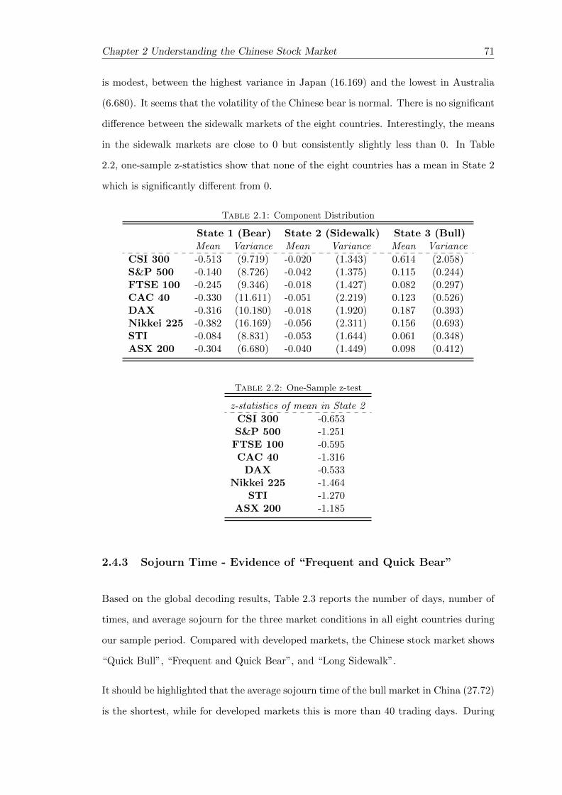
Chapter 2 Understanding the Chinese Stock Market 71
is modest, between the highest variance in Japan (16.169) and the lowest in Australia
(6.680). It seems that the volatility of the Chinese bear is normal. There is no significant
difference between the sidewalk markets of the eight countries. Interestingly, the means
in the sidewalk markets are close to 0 but consistently slightly less than 0. In Table
2.2, one-sample z-statistics show that none of the eight countries has a mean in State 2
which is significantly different from 0.
Table 2.1: Component Distribution
State 1 (Bear) State 2 (Sidewalk) State 3 (Bull)Mean Variance Mean Variance Mean Variance
CSI 300 -0.513 (9.719) -0.020 (1.343) 0.614 (2.058)S&P 500 -0.140 (8.726) -0.042 (1.375) 0.115 (0.244)FTSE 100 -0.245 (9.346) -0.018 (1.427) 0.082 (0.297)CAC 40 -0.330 (11.611) -0.051 (2.219) 0.123 (0.526)DAX -0.316 (10.180) -0.018 (1.920) 0.187 (0.393)Nikkei 225 -0.382 (16.169) -0.056 (2.311) 0.156 (0.693)STI -0.084 (8.831) -0.053 (1.644) 0.061 (0.348)ASX 200 -0.304 (6.680) -0.040 (1.449) 0.098 (0.412)
Table 2.2: One-Sample z-test
z-statistics of mean in State 2
CSI 300 -0.653S&P 500 -1.251FTSE 100 -0.595CAC 40 -1.316
DAX -0.533Nikkei 225 -1.464
STI -1.270ASX 200 -1.185
2.4.3 Sojourn Time - Evidence of “Frequent and Quick Bear”
Based on the global decoding results, Table 2.3 reports the number of days, number of
times, and average sojourn for the three market conditions in all eight countries during
our sample period. Compared with developed markets, the Chinese stock market shows
“Quick Bull”, “Frequent and Quick Bear”, and “Long Sidewalk”.
It should be highlighted that the average sojourn time of the bull market in China (27.72)
is the shortest, while for developed markets this is more than 40 trading days. During
72 Chapter 2 Understanding the Chinese Stock Market
our sample period, the Chinese market was in the bull market for 693 trading days, but
entered and exited the bull market 25 times. We observe that the United States is also
in the bull market a large number of times (27). However, the total number of days the
United States is in the bull market (1133) is nearly double that of China, which results
in a relatively longer average sojourn in the bull market (41.96).
China, along with the United Kingdom and Japan, are found to have a short average
sojourn in the bear market, whilst the other five countries have more than 30 trading
days. It should be pointed out that China was in the bear market 22 times, while all of
the other countries were around five times in the bear market in our sample period. We
can argue that the “Quick Bear” happens in the United Kingdom and Japan but not
frequently, while China has a “Frequent and Quick Bear”.
The average sojourn of the sidewalk market in China is 230.17, more than twice that of
other countries. Additionally, China was only in the sidewalk market six times in the
sample period. Every time China entered the sidewalk market, the long-term trend in
the stock market cannot be established unless the long sojourn in the sidewalk market
has elapsed. The most obvious sidewalk period in China is from 2011 to 2014, where
the CSI 300 stayed roughly between 2000 and 3000. During that period, whenever the
CSI 300 was near the ceiling or floor, it would eventually return to the band again.
2.4.4 Transition Probability Matrix - Evidence of “No Buffer Zone”
We found a very unique characteristic, “No Buffer Zone”, of the Chinese stock market
from the estimated transition probability matrix in Table 2.4. The direct transition
probability from the bear market to bull market (or the opposite direction) is close to
0% in all developed markets. It is clearly shown that all developed markets always have
the sidewalk market as a buffer zone between the bull and bear market. Nevertheless, the
transition probability matrix in China is very special with a particularly high transition
probability from the bear market to the bull market (nearly 100%) and a relatively
high transition probability from the bull market to the bear market (77.05%). The
buffer zone effect was not found to exist in China over the sample period. The direct
transition between the bull market and the bear market is typical. It was found that the
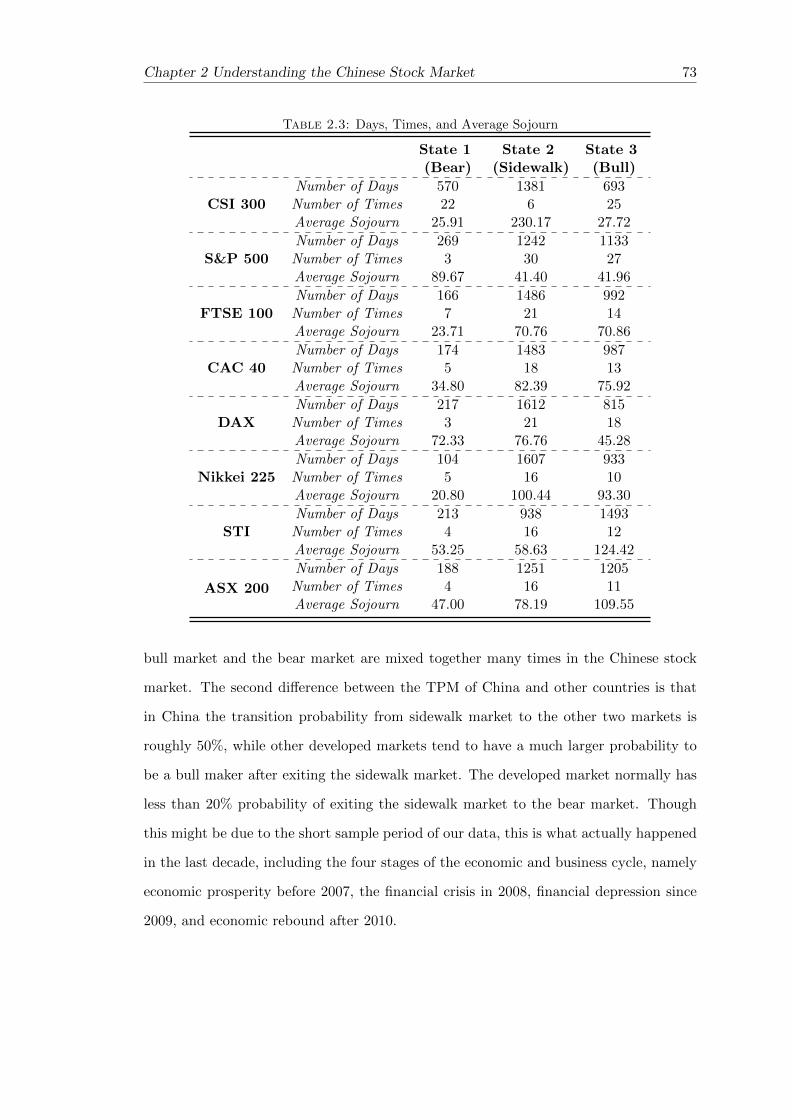
Chapter 2 Understanding the Chinese Stock Market 73
Table 2.3: Days, Times, and Average Sojourn
State 1 State 2 State 3(Bear) (Sidewalk) (Bull)
CSI 300Number of Days 570 1381 693
Number of Times 22 6 25Average Sojourn 25.91 230.17 27.72
S&P 500Number of Days 269 1242 1133
Number of Times 3 30 27Average Sojourn 89.67 41.40 41.96
FTSE 100Number of Days 166 1486 992
Number of Times 7 21 14Average Sojourn 23.71 70.76 70.86
CAC 40Number of Days 174 1483 987
Number of Times 5 18 13Average Sojourn 34.80 82.39 75.92
DAXNumber of Days 217 1612 815
Number of Times 3 21 18Average Sojourn 72.33 76.76 45.28
Nikkei 225Number of Days 104 1607 933
Number of Times 5 16 10Average Sojourn 20.80 100.44 93.30
STINumber of Days 213 938 1493
Number of Times 4 16 12Average Sojourn 53.25 58.63 124.42
ASX 200
Number of Days 188 1251 1205Number of Times 4 16 11Average Sojourn 47.00 78.19 109.55
bull market and the bear market are mixed together many times in the Chinese stock
market. The second difference between the TPM of China and other countries is that
in China the transition probability from sidewalk market to the other two markets is
roughly 50%, while other developed markets tend to have a much larger probability to
be a bull maker after exiting the sidewalk market. The developed market normally has
less than 20% probability of exiting the sidewalk market to the bear market. Though
this might be due to the short sample period of our data, this is what actually happened
in the last decade, including the four stages of the economic and business cycle, namely
economic prosperity before 2007, the financial crisis in 2008, financial depression since
2009, and economic rebound after 2010.
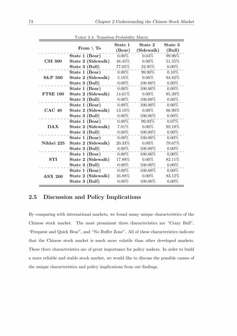
74 Chapter 2 Understanding the Chinese Stock Market
Table 2.4: Transition Probability Matrix
From \ ToState 1 State 2 State 3(Bear) (Sidewalk) (Bull)
CSI 300State 1 (Bear) 0.00% 0.04% 99.96%State 2 (Sidewalk) 48.45% 0.00% 51.55%State 3 (Bull) 77.05% 22.95% 0.00%
S&P 500State 1 (Bear) 0.00% 99.90% 0.10%State 2 (Sidewalk) 5.18% 0.00% 94.82%State 3 (Bull) 0.00% 100.00% 0.00%
FTSE 100State 1 (Bear) 0.00% 100.00% 0.00%State 2 (Sidewalk) 14.61% 0.00% 85.39%State 3 (Bull) 0.00% 100.00% 0.00%
CAC 40State 1 (Bear) 0.00% 100.00% 0.00%State 2 (Sidewalk) 13.10% 0.00% 86.90%State 3 (Bull) 0.00% 100.00% 0.00%
DAXState 1 (Bear) 0.00% 99.93% 0.07%State 2 (Sidewalk) 7.81% 0.00% 92.19%State 3 (Bull) 0.00% 100.00% 0.00%
Nikkei 225State 1 (Bear) 0.00% 100.00% 0.00%State 2 (Sidewalk) 20.33% 0.00% 79.67%State 3 (Bull) 0.00% 100.00% 0.00%
STIState 1 (Bear) 0.00% 100.00% 0.00%State 2 (Sidewalk) 17.89% 0.00% 82.11%State 3 (Bull) 0.00% 100.00% 0.00%
ASX 200
State 1 (Bear) 0.00% 100.00% 0.00%State 2 (Sidewalk) 16.88% 0.00% 83.12%State 3 (Bull) 0.00% 100.00% 0.00%
2.5 Discussion and Policy Implications
By comparing with international markets, we found many unique characteristics of the
Chinese stock market. The most prominent three characteristics are “Crazy Bull”,
“Frequent and Quick Bear”, and “No Buffer Zone”. All of these characteristics indicate
that the Chinese stock market is much more volatile than other developed markets.
These three characteristics are of great importance for policy makers. In order to build
a more reliable and stable stock market, we would like to discuss the possible causes of
the unique characteristics and policy implications from our findings.

Chapter 2 Understanding the Chinese Stock Market 75
2.5.1 “Crazy Bull” - Rational Security Analysis and Adjust Investor
Structure
Compared with other developed markets, the Chinese stock market has considerably
high variance in the bull market, which could be induced by the herding behaviour of
individual investors. Kim & Wei (2002) provide evidence that individual investors are
more likely to engage in herding. Kumar & Lee (2006) use more than 1.85 million
individual investor transaction at a major US discount brokerage house to show that
individual investors buy or sell stocks in concert during 1991-1996. Moreover, they
can be easily influenced by news and market sentiment. Barber & Odean (2008) test
and confirm that individual investors are net buyers of stocks in the news with public
attention.
In order to mitigating the herding behaviour, Lao & Singh (2011) suggest that large
financial institutions can bring more rational security analysis to the general public,
which can decrease the level of speculative investments activity by the individual in-
vestors. Most individual investors have little knowledge of stock markets and focus on
speculation of short-term price changes, rather than the fundamental value of listed
companies. It is imperative to guide individual investors to focus on the fundamental
values of firms and encourage individual investors to make rational investments.
In China, individual investors account for 82.24% of total trading volume in 2013 (Han
& Li, 2017), whereas institutional investors dominate in developed markets. Boehmer
& Kelley (2009) show that stock with greater institutional ownership are priced more
efficiently. The Chinese government needs to adjust investor structure and promote
the development of institutional investors, like asset management firms, private funds,
and mutual funds. Institutional investors have expert knowledge and skills to manage
professional investments that seek long-term returns under the proper risk management.
2.5.2 “Frequent and Quick Bear” - Risk Management Tools
In China, the bear market is quick and occurs more frequently than in developed markets.
As a matter of fact, short-selling is limited in the Chinese stock market. Most investors
76 Chapter 2 Understanding the Chinese Stock Market
can only buy stocks in China. Mei et al. (2009) point out that the mispricing can hardly
be arbitrage away at both the market level and the individual stock level in a market
with the stringent constraints on short selling. It is very difficult to hedge downside risk
during the bear market.
Index futures Contracts are appropriate tools to hedge downside risk during a bear
market. Lien & Tse (2000) utilize the futures contracts to develop a hedge strategy
that minimizes the lower partial moments. Lien & Tse (2002) review the theoretical
background and the econometric implementation of various futures hedging. Chen et al.
(2003) investigate different theoretical methods to the optimal futures hedge ratios.
Although the China Financial Futures Exchange launched the first index futures con-
tracts, the CSI 300 index futures, on April 16th 2010, the trading of index futures
are under strict restrictions. Firstly, there are high barriers for individual investors to
participant because of the high deposit requirement and the minimum account size re-
quirement. Secondly, the margin requirements are 15% to 18%, which is much higher
than the margin requirement of index futures in developed countries. Thirdly, QFIIs
were not eligible to trade the index futures.
In July 2015, more restrictions on index future trading have hampered the development
of financial markets. The most strict rule was that the number of opening contracts
can not more than 10 per day. This rule made investors to use the index futures to
manage risk. In order to develop the Chinese stock market, it is crucial to remove the
restrictions on the trading of domestic index future products for investors to hedge the
downside risk during the frequent bear market. In this way, the Chinese stock market
can stay on the promised path of reform to become more market-oriented rather than
policy-oriented.
2.5.3 “No Buffer Zone” - Restriction on Leverage
The most notable characteristic of the Chinese stock market is that the bull market
is typically mixed with the bear market and that there is no sidewalk market between
them. In developed markets, the sidewalk market always functions as the “buffer zone”
Chapter 2 Understanding the Chinese Stock Market 77
between the bear market and the bull market. The “No Buffer Zone” phenomenon can
be explained by the overreaction effect in behavioural finance. DeBondt & Thaler (1985)
find that most investors usually overreact to unexpected and dramatic news, suggesting
the weak from market inefficiencies. Wang et al. (2004) study the overreaction effect in
China during the period between 1994 to 2000 and find that the overreaction effect is
most pronounced in A-share market.
More importantly, Hsu (2015) point out that the excess leverage from other source
financing exaggerated the effect of the overreaction in China. In 2015, the Chinese stock
market encountered a bull market followed by a bear market, which increased volatility to
a historically high level. It is highly likely that the abnormally high volatility was caused
by excess leverage, specifically through other source financing, like umbrella trusts and
fund-matching companies (Hsu, 2015). By margin loan and margin financing, brokerages
can increase funding by up to twice the margin (i.e. ratio at 1:2). Through umbrella
trusts, one could leverage up to five times the margin (i.e. ratio at 1:5).
The excess leverage of other source financing exaggerates the downside risk of the Chinese
stock market, which caused the contagion of the market crisis. It is inevitable that
detailed regulation needs to be imposed on umbrella trusts and fund-matching companies
(Tian, 2015). There should be strict rules in the banking sector to provide funding for
umbrella trusts (Jiang, 2014). Leverage should be capped at a much lower level. The
monitoring of fund-matching companies needs to be significantly reinforced. Finally,
information on other source financing should be more transparent to the public.
2.6 Conclusion
The definition of bear, sidewalk, and bull markets is ambiguous in existing literature.
This makes it difficult for practitioners to distinguish between different market condi-
tions. In this chapter, we employ a statistical definition of bear, sidewalk, and bull mar-
kets, which correspond to the three states in our hidden semi-Markov model. Through
the comparison with seven developed markets, we found three unique characteristics of

78 Chapter 2 Understanding the Chinese Stock Market
the Chinese stock market, namely “Crazy Bull”, “Frequent and Quick Bear”, and “No
Buffer Zone”.
“Crazy Bull” refers to the fact that the variance of the bull market in the Chinese stock
market is noticeably higher than for developed markets. “Frequent and Quick Bear”
is implied by the fact that the bull market occurs frequently in China and the sojourn
time of the Chinese bull market is short. “No Buffer Zone” is the most prominent
characteristic. It is observed that the sidewalk in developed markets always functions as
a buffer zone between the bear and bull markets, while this case never occurs in China.
The possible causes of those three characteristics were discussed. Based on the discus-
sion, it is very important to adjust the investor structure, to provide risk management
tools, and to strengthen supervision on the excess leverage from other source financing.

Chapter 3
Asset Return & Camel Process:
Beauty and the Beast
In this chapter, we propose a new diffusion process referred to as the “camel process”
in order to model the cumulative return of a financial asset. The process considers the
market condition and the price reversal. This new process includes three parameters, the
market condition parameter α, the price reversal parameter β, the volatility parameter
γ. Its steady state probability density function could be unimodal or bimodal, depending
on the sign of the market condition parameter. The price reversal is realised through the
non-linear drift term which incorporates the cube term of the instantaneous cumulative
return. The time-dependent solution of its Fokker-Planck equation cannot be obtained
analytically, but can be numerically solved using the finite difference method. The proper-
ties of the camel process are confirmed by our empirical estimation results of ten market
indexes in two different periods.
79

80 Chapter 3 Asset Return & Camel Process
3.1 Introduction
Diffusion processes have been widely used in the asset pricing. One of most popular
parametric diffusion process is the geometric Brownian motion in the Black-Scholes
model (see Black & Scholes, 1973; Merton, 1973). The geometric Brownian motion
has the assumption of independent multiplicative increments, which is often violated
by the empirical observation of the asset returns, i.e. stylized facts of asset returns.
Many other parametric diffusion processes have been developed to improve the Black-
Scholes by explaining the stylized facts (e.g. Mandelbrot, 1997; Jackel, 2004; Bingham
& Kiesel, 2001; Eberlein & Keller, 1995; Merton, 1976). To the best of our knowledge,
there is no parametric diffusion process considering the market condition and the price
reversal, although they have been widely studied in the literature of technical analysis
and behavioural finance. Our new proposed “camel process” contributes to the fill this
literature gap.
Financial economists often argue that asset price may behaves differently in different
market conditions. Levy (1974) suggest to estimate separate beta coefficients for bull
and bear market. Not all study are in favour of different behaviours in different mar-
ket conditions. Fabozzi & Francis (1977) conclude the coefficients of the sing-index
market model are not significantly different in three types of market condition defi-
nition, Bull and Bear, Up and Down, Substantial Up and Down. However, Kim &
Zumwalt (1979) extend the design of Fabozzi & Francis (1977) and show the evidence
that more stock exhibited significantly difference between Up-market and Dow-market
betas. Chen (1982) uses the time-varying beta approach to avoid the multicollinearity
problem in Kim & Zumwalt (1979) and re-examine the difference in Up-market and
Dow-market betas. The results obtained from time-varying beta approach is consistent
with Kim & Zumwalt (1979) and support that betas tend to be different in Up-market
and Down-market. Using three-state hidden semi-Markov Model, Chapter 1 has shown
that asset returns follow different distributions in different market conditions. To the
best of our knowledge again, there is no diffusion process in the finance study considering
the market condition.
Chapter 3 Asset Return & Camel Process 81
Additionally, the violation of EMH can often be explained by behavioural finance. One
of the important explanation is the overreaction hypothesis 1 that investors tend to
overreact to new information, such as positive and negative shocks. The overreaction
can be observed at the individual stock level (Keynes, 1964; Williams, 1938; Arrow,
1982) as well as the market level (DeBondt & Thaler, 1985; De Bondt & Thaler, 1987).
Additionally, the overreaction can occur at the short-term (Zarowin, 1989; Atkins &
Dyl, 1990; Cox & Peterson, 1994) as well as the long-term (DeBondt & Thaler, 1985;
Loughran & Ritter, 1996; Campbell & Limmack, 1997). Price reversal is the phenomenon
after the overreaction because stock prices tend to converge back to the fundamental
values. The price reversal has been widely empirically studied in different markets
(Bremer & Sweeney, 1991; Liang & Mullineaux, 1994; Farag, 2014). To the best of our
knowledge, no diffusion process in the finance study has considered the price reversal.
In this chapter, we propose a new diffusion process referred to as the “camel process”
in order to model the cumulative return of a financial asset. The camel process has
two contributions. First, it is capable of modelling the cumulative return in two market
conditions, either sidewalk or trending2. Second, the process consider the price reversal
after the long-term overreaction behaviour in the financial market. The form of the
camel process is parsimonious with three parameters, the market condition parameter
α, the price reversal parameter β, and the volatility parameter γ. The market condition
can be identified by the sign of α. The magnitude of price reversal is measured by β. γ
controls the level of volatility.
The beauty of the camel process is that it considers the market condition and the price
reversal. The beast is that the time-dependent solution cannot be obtained analytically,
but can be numerically solved by means of a finite difference method. The name of the
“camel process” is inspired by its property indicating that the steady state probability
density function (PDF) could be unimodal or bimodal, depending on the sign of the
1It is not always overreaction, but sometimes be slow or underreaction. Hong & Stein (1999) constructa model with two groups of boundedly rational agents “newwatchers” and “momentum traders” andshow the underreaction at short horizons and overreaction at long horizons. Fama (1998) claims thatoverreaction to information is as frequent as underreaction. Veronesi (1999) uses a dynamic, rationalexpectations equilibrium model of asset prices to demonstrate that stock prices underreact to good newsin bad times and overreact to bad news in good times.
2A trending market includes both the bull market and the bear market.

82 Chapter 3 Asset Return & Camel Process
market condition parameter. The price reversal is realised through the non-linear drift
term which incorporates the cube term of the instantaneous cumulative return.
3.2 Literature Review
In this section, we summarize alternative models to the Black-Scholes model. The
existing literature attempted to improve the Black-Scholes by explaining the stylized
facts of asset returns. It is well documented that empirical daily returns have stylized
facts which are the heavy-tails, the “long-memory”, the volatility clustering, the Taylor
effect, and so forth. (see Granger & Ding, 1995; Pagan, 1996; Cont, 2001). Those
stylized facts indicate that the independent normality assumption in the Black-Scholes
model is unrealistic. In order to explain the stylized facts, many research studies have
been devoted to modifying the Geometric Brownian motion used in the derivation of
the Black-Scholes model.
The first type of alternative models is represented by the fractional Brownian motions.
Mandelbrot (1997) argues that successive price changes are not independent, and em-
ploys the fractional Brownian motion to capture the dependent increments. In the
finance study, a model should be self-consistent and show no arbitrage opportunity
(Kou, 2007). Nevertheless, Rogers (1997) proves that the fractional Brownian motion is
not semi-martingale and shows the construction of arbitrage in the fractional Brownian
motion.
The stochastic volatility and GARCH models are developed to capture the stylized
fact of volatility clustering. Jackel (2004) reviews various stochastic volatility models
with a focus on the dynamic replication of exotic derivatives and their implementation.
Bollerslev et al. (1992) provides a comprehensive review on the ARCH-family models. In
addition to the price process, these models introduce another process for the evolution
of volatility so that the time dependence of volatility could be captured.
Bingham & Kiesel (2001) asserts that the hyperbolic model is a good choice if someone
wants a model that is more complex than the benchmark Black-Scholes model, but less
Chapter 3 Asset Return & Camel Process 83
complicated than the stochastic volatility models. Hyperbolic diffusion models are de-
signed due to the empirical evidence that the hyperbolic distributions could be fitted to
daily returns with high accuracy (Eberlein & Keller, 1995). These models use hyper-
bolic distributions rather than normal distributions. Bibby & Sørensen (1996) models
the logarithm of the stock price by an ergodic process using the hyperbolic invariance
measure, but their simulation shows that there is no significant difference between the
option price inferred by the hyperbolic diffusion model and by the Black-Scholes model.
Merton (1976) derives an option pricing formula based on the assumption that the
underlying stock returns are generated by the combination of continuous and jump pro-
cesses. The abnormally large empirical returns can be explained by the jump-diffusion
model, which can also replicate the heavy tails of the daily return distribution. Kou
(2002) proposes a double exponential jump-diffusion model which gives analytical so-
lutions for path-dependent options. Cont & Tankov (2004) reviews the models based
on the jump processes. There are some other alternative models, namely the “implied
binomial tress” (Dupire et al., 1994), time changed Levy process (Carr et al., 2003), and
the affine jump-diffusion models (Duffie et al., 2000).
The reminder of the chapter is structured as follows. Section 3.3 defines the camel
process and discusses its properties. Section 3.4 presents empirical estimation results of
ten market indexes in two different periods. Section 3.5 summarises the chapter.
3.3 The SDE and its properties
The “camel process” captures the dynamically non-linear interaction between the in-
crement of the cumulative return and the instantaneous cumulative return with the
consideration of the market condition and the price reversal. The non-linear relation-
ship is achieved by the inclusion of the cube term of the instantaneous cumulative return,
which facilitates the modelling of price reversal after the overreaction behaviour. The
sign of drift term is determined by the market condition, whether the cumulative return
deviating from zero in the trending market condition or moving towards zero in the
sidewalk market condition. The camel process is defined as:
84 Chapter 3 Asset Return & Camel Process
Definition 3.1. The camel process solves the stochastic differential equation (SDE)
dXt = (αXt − βX3t ) dt+ γ dWt , X0 = 0 (3.1)
where α, β, and γ are three parameters with α ∈ R, β ∈ R≥0, and γ ∈ R+.
Parameter α is referred to as the market condition parameter. If α > 0, the market is in
a trending market condition. Otherwise, it is in a sidewalk market condition. Parameter
β controls the price reversal after the overreaction behaviour in the market. If there is
no overreaction, β is essentially zero. Parameter γ measures the volatility of the process.
In the camel process, the volatility is constant. In terms of the parameter space, α can
be any real number, β is a non-negative real number, and γ can only be a positive real
number. Since the underlying process modelled is the cumulative return, the process
always starts at zero.
We investigate the cumulative return rather than the price or the log price for two rea-
sons. First, the overreaction can be easily measured by the cumulative return. Second,
the cumulative return facilitates the comparison of investments in different financial
assets.
The cumulative return investigated by us is defined as
Xt =t∑i=1
ri (3.2)
where ri is the log return 3 of the price process {Pt, t ≥ 0} of the asset
ri = log(Pt)− log(Pt−1) (3.3)
3.3.1 Steady State PDF
It is difficult to analytically obtain the solution of the camel process due to its high order
non-linear term. We here use the Fokker-Planck equation to conduct a partial analytic
3Like most researches, we prefer the log return rather than the arithmetic return Yi = (Pt −Pt−1)/Pt−1. The reason is that the cumulative return over an n period is the sum of the log return(shown in Equation 3.2), while the arithmetic return does not have this property.
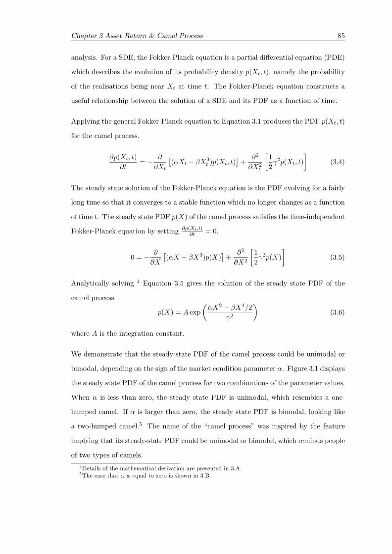
Chapter 3 Asset Return & Camel Process 85
analysis. For a SDE, the Fokker-Planck equation is a partial differential equation (PDE)
which describes the evolution of its probability density p(Xt, t), namely the probability
of the realisations being near Xt at time t. The Fokker-Planck equation constructs a
useful relationship between the solution of a SDE and its PDF as a function of time.
Applying the general Fokker-Planck equation to Equation 3.1 produces the PDF p(Xt, t)
for the camel process.
∂p(Xt, t)
∂t= − ∂
∂Xt
[(αXt − βX3
t )p(Xt, t)]
+∂2
∂X2t
[1
2γ2p(Xt, t)
](3.4)
The steady state solution of the Fokker-Planck equation is the PDF evolving for a fairly
long time so that it converges to a stable function which no longer changes as a function
of time t. The steady state PDF p(X) of the camel process satisfies the time-independent
Fokker-Planck equation by setting ∂p(Xt,t)∂t = 0.
0 = − ∂
∂X
[(αX − βX3)p(X)
]+
∂2
∂X2
[1
2γ2p(X)
](3.5)
Analytically solving 4 Equation 3.5 gives the solution of the steady state PDF of the
camel process
p(X) = A exp
(αX2 − βX4/2
γ2
)(3.6)
where A is the integration constant.
We demonstrate that the steady-state PDF of the camel process could be unimodal or
bimodal, depending on the sign of the market condition parameter α. Figure 3.1 displays
the steady state PDF of the camel process for two combinations of the parameter values.
When α is less than zero, the steady state PDF is unimodal, which resembles a one-
humped camel. If α is larger than zero, the steady state PDF is bimodal, looking like
a two-humped camel.5 The name of the “camel process” was inspired by the feature
implying that its steady-state PDF could be unimodal or bimodal, which reminds people
of two types of camels.
4Details of the mathematical derivation are presented in 3.A.5The case that α is equal to zero is shown in 3.B.
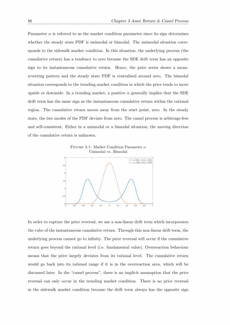
86 Chapter 3 Asset Return & Camel Process
Parameter α is referred to as the market condition parameter since its sign determines
whether the steady state PDF is unimodal or bimodal. The unimodal situation corre-
sponds to the sidewalk market condition. In this situation, the underlying process (the
cumulative return) has a tendency to zero because the SDE drift term has an opposite
sign to its instantaneous cumulative return. Hence, the price series shows a mean-
reverting pattern and the steady state PDF is centralised around zero. The bimodal
situation corresponds to the trending market condition in which the price tends to move
upside or downside. In a trending market, a positive α generally implies that the SDE
drift term has the same sign as the instantaneous cumulative return within the rational
region. The cumulative return moves away from the start point, zero. In the steady
state, the two modes of the PDF deviate from zero. The camel process is arbitrage-free
and self-consistent. Either in a unimodal or a bimodal situation, the moving direction
of the cumulative return is unknown.
Figure 3.1: Market Condition Parameter αUnimodal vs. Bimodal
-1 -0.8 -0.6 -0.4 -0.2 0 0.2 0.4 0.6 0.8 10
0.5
1
1.5
2
2.5
3α=0.05; β=0.2; γ=0.05α=-0.05; β=0.2; γ=0.05
In order to capture the price reversal, we use a non-linear drift term which incorporates
the cube of the instantaneous cumulative return. Through this non-linear drift term, the
underlying process cannot go to infinity. The price reversal will occur if the cumulative
return goes beyond the rational level (i.e. fundamental value). Overreaction behaviour
means that the price largely deviates from its rational level. The cumulative return
would go back into its rational range if it is in the overreaction area, which will be
discussed later. In the “camel process”, there is an implicit assumption that the price
reversal can only occur in the trending market condition. There is no price reversal
in the sidewalk market condition because the drift term always has the opposite sign

Chapter 3 Asset Return & Camel Process 87
as the instantaneous cumulative return in the sidewalk market condition, which will be
discussed in detail later.
Parameter β is the parameter which controls the price reversal. Figure 3.2 displays the
steady state PDF of both the sidewalk and trending market condition. There is no big
effect of the price reversal parameter β on the steady state PDF when the market is in
sidewalk. However, the effect of β is vital if the market is in the trending state. A larger
value of β forces the mode of the steady state PDF more close to zero. In contrast, the
mode of the steady state PDF can move further away if β is small.
The price reversal is realised through the non-linear drift term αXt − βX3t . Figure 3.3
shows the shape of the non-linear drift term under both market conditions. In a sidewalk
market condition, the drift term always has the opposite sign as the instantaneous
cumulative return. Hence, the cumulative return moves towards to zero and shows the
mean-reverting pattern. Under this situation, the price reversal normally rarely occurs.
However, the price reversal plays a vital role in the trending market condition. As you
can see in the lower panel of Figure 3.3, there is a middle region that the drift term has
the same sign as the instantaneous cumulative return. There are other two side regions
indicating that the sign is opposite. The two side regions are deemed as the overreaction
area. If the cumulative return goes into the overreaction area, the drift term would force
it to move back the rational region, which is the one in the middle.
The range of the rational region is controlled by parameter β. If the value of β is large,
then the magnitude of the price reversal is stronger and the rational region is narrower.
Conversely, a smaller β means that the market can tolerate overreaction to a larger
extent. Thus, the range of the rational region is wider.
Parameter γ is known as the volatility parameter. It controls the volatility magnitude
of dWt. Figure 3.4 illustrates that the steady state PDF is more diversified with a larger
value of γ. By contrast, a smaller value of γ results in a more centralised steady state
PDF. Importantly, the mode of the steady state PDF remains the same irrespective of
the change of the value of γ under both unimodal or bimodal situations. The mode
of the steady state PDF only depends on the market condition parameter α and the
overreaction parameter β.
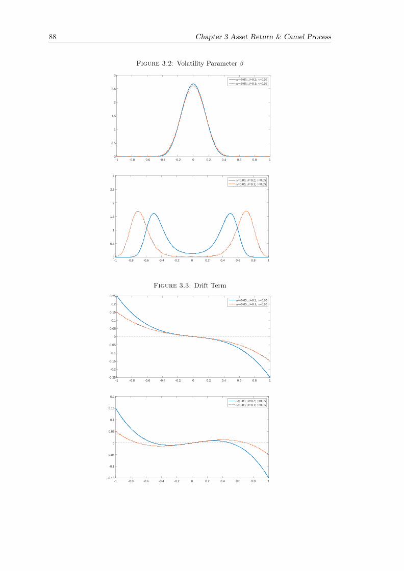
88 Chapter 3 Asset Return & Camel Process
Figure 3.2: Volatility Parameter β
-1 -0.8 -0.6 -0.4 -0.2 0 0.2 0.4 0.6 0.8 10
0.5
1
1.5
2
2.5
3α=-0.05; β=0.2; γ=0.05α=-0.05; β=0.1; γ=0.05
-1 -0.8 -0.6 -0.4 -0.2 0 0.2 0.4 0.6 0.8 10
0.5
1
1.5
2
2.5
3α=0.05; β=0.2; γ=0.05α=0.05; β=0.1; γ=0.05
Figure 3.3: Drift Term
-1 -0.8 -0.6 -0.4 -0.2 0 0.2 0.4 0.6 0.8 1-0.25
-0.2
-0.15
-0.1
-0.05
0
0.05
0.1
0.15
0.2
0.25α=-0.05; β=0.2; γ=0.05α=-0.05; β=0.1; γ=0.05
-1 -0.8 -0.6 -0.4 -0.2 0 0.2 0.4 0.6 0.8 1-0.15
-0.1
-0.05
0
0.05
0.1
0.15
0.2α=0.05; β=0.2; γ=0.05α=0.05; β=0.1; γ=0.05
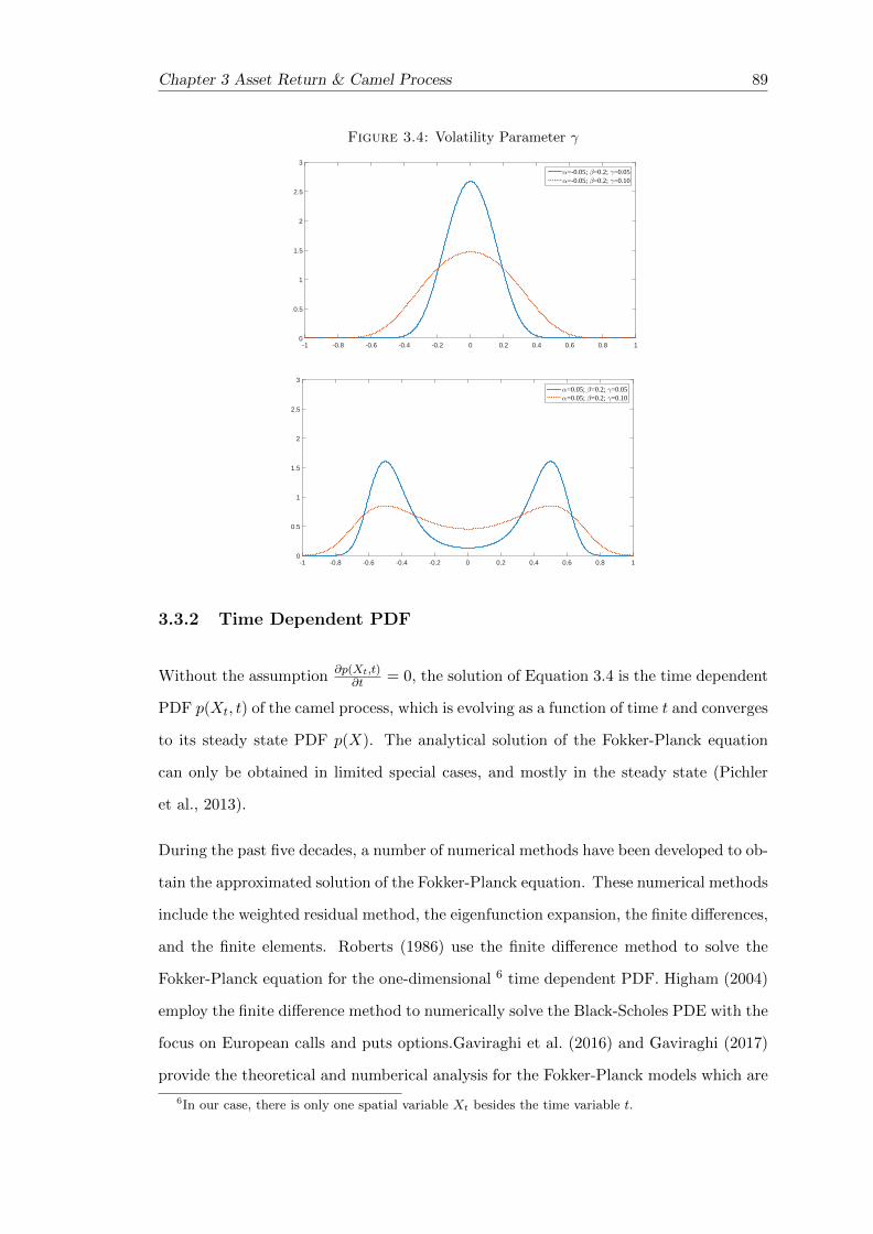
Chapter 3 Asset Return & Camel Process 89
Figure 3.4: Volatility Parameter γ
-1 -0.8 -0.6 -0.4 -0.2 0 0.2 0.4 0.6 0.8 10
0.5
1
1.5
2
2.5
3α=-0.05; β=0.2; γ=0.05α=-0.05; β=0.2; γ=0.10
-1 -0.8 -0.6 -0.4 -0.2 0 0.2 0.4 0.6 0.8 10
0.5
1
1.5
2
2.5
3α=0.05; β=0.2; γ=0.05α=0.05; β=0.2; γ=0.10
3.3.2 Time Dependent PDF
Without the assumption ∂p(Xt,t)∂t = 0, the solution of Equation 3.4 is the time dependent
PDF p(Xt, t) of the camel process, which is evolving as a function of time t and converges
to its steady state PDF p(X). The analytical solution of the Fokker-Planck equation
can only be obtained in limited special cases, and mostly in the steady state (Pichler
et al., 2013).
During the past five decades, a number of numerical methods have been developed to ob-
tain the approximated solution of the Fokker-Planck equation. These numerical methods
include the weighted residual method, the eigenfunction expansion, the finite differences,
and the finite elements. Roberts (1986) use the finite difference method to solve the
Fokker-Planck equation for the one-dimensional 6 time dependent PDF. Higham (2004)
employ the finite difference method to numerically solve the Black-Scholes PDE with the
focus on European calls and puts options.Gaviraghi et al. (2016) and Gaviraghi (2017)
provide the theoretical and numberical analysis for the Fokker-Planck models which are
6In our case, there is only one spatial variable Xt besides the time variable t.
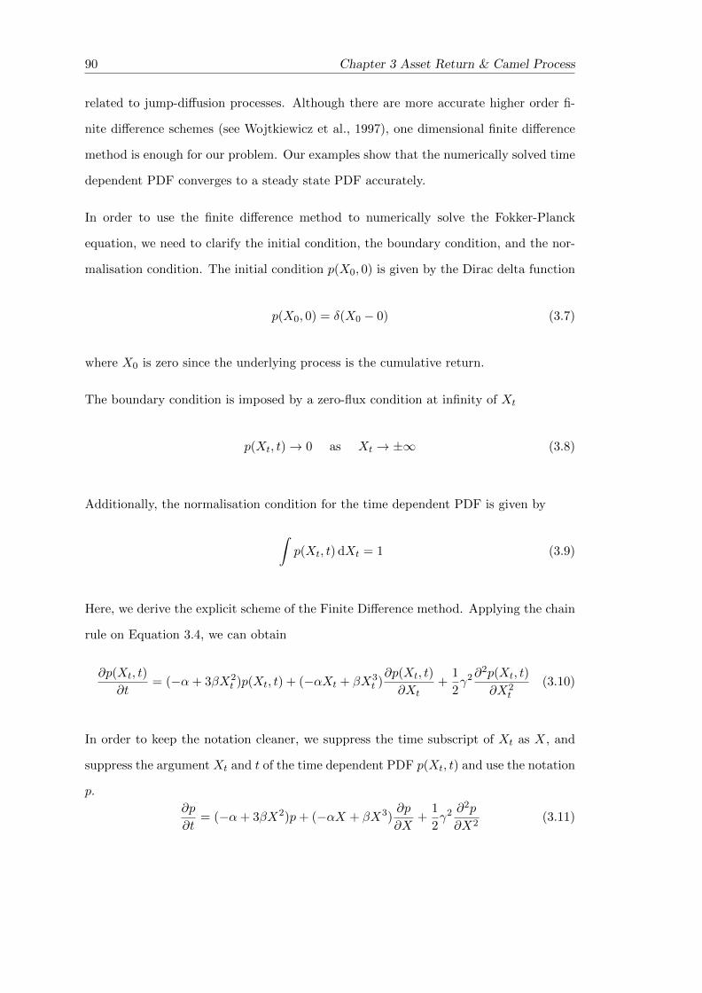
90 Chapter 3 Asset Return & Camel Process
related to jump-diffusion processes. Although there are more accurate higher order fi-
nite difference schemes (see Wojtkiewicz et al., 1997), one dimensional finite difference
method is enough for our problem. Our examples show that the numerically solved time
dependent PDF converges to a steady state PDF accurately.
In order to use the finite difference method to numerically solve the Fokker-Planck
equation, we need to clarify the initial condition, the boundary condition, and the nor-
malisation condition. The initial condition p(X0, 0) is given by the Dirac delta function
p(X0, 0) = δ(X0 − 0) (3.7)
where X0 is zero since the underlying process is the cumulative return.
The boundary condition is imposed by a zero-flux condition at infinity of Xt
p(Xt, t)→ 0 as Xt → ±∞ (3.8)
Additionally, the normalisation condition for the time dependent PDF is given by
∫p(Xt, t) dXt = 1 (3.9)
Here, we derive the explicit scheme of the Finite Difference method. Applying the chain
rule on Equation 3.4, we can obtain
∂p(Xt, t)
∂t= (−α+ 3βX2
t )p(Xt, t) + (−αXt + βX3t )∂p(Xt, t)
∂Xt+
1
2γ2∂
2p(Xt, t)
∂X2t
(3.10)
In order to keep the notation cleaner, we suppress the time subscript of Xt as X, and
suppress the argument Xt and t of the time dependent PDF p(Xt, t) and use the notation
p.
∂p
∂t= (−α+ 3βX2)p+ (−αX + βX3)
∂p
∂X+
1
2γ2 ∂
2p
∂X2(3.11)
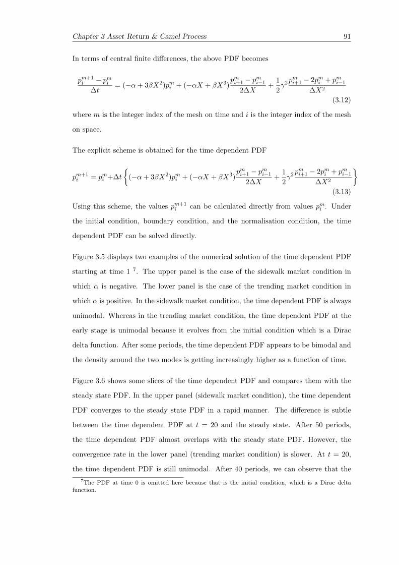
Chapter 3 Asset Return & Camel Process 91
In terms of central finite differences, the above PDF becomes
pm+1i − pmi
∆t= (−α+ 3βX2)pmi + (−αX + βX3)
pmi+1 − pmi−1
2∆X+
1
2γ2 p
mi+1 − 2pmi + pmi−1
∆X2
(3.12)
where m is the integer index of the mesh on time and i is the integer index of the mesh
on space.
The explicit scheme is obtained for the time dependent PDF
pm+1i = pmi +∆t
{(−α+ 3βX2)pmi + (−αX + βX3)
pmi+1 − pmi−1
2∆X+
1
2γ2 p
mi+1 − 2pmi + pmi−1
∆X2
}(3.13)
Using this scheme, the values pm+1i can be calculated directly from values pmi . Under
the initial condition, boundary condition, and the normalisation condition, the time
dependent PDF can be solved directly.
Figure 3.5 displays two examples of the numerical solution of the time dependent PDF
starting at time 1 7. The upper panel is the case of the sidewalk market condition in
which α is negative. The lower panel is the case of the trending market condition in
which α is positive. In the sidewalk market condition, the time dependent PDF is always
unimodal. Whereas in the trending market condition, the time dependent PDF at the
early stage is unimodal because it evolves from the initial condition which is a Dirac
delta function. After some periods, the time dependent PDF appears to be bimodal and
the density around the two modes is getting increasingly higher as a function of time.
Figure 3.6 shows some slices of the time dependent PDF and compares them with the
steady state PDF. In the upper panel (sidewalk market condition), the time dependent
PDF converges to the steady state PDF in a rapid manner. The difference is subtle
between the time dependent PDF at t = 20 and the steady state. After 50 periods,
the time dependent PDF almost overlaps with the steady state PDF. However, the
convergence rate in the lower panel (trending market condition) is slower. At t = 20,
the time dependent PDF is still unimodal. After 40 periods, we can observe that the
7The PDF at time 0 is omitted here because that is the initial condition, which is a Dirac deltafunction.
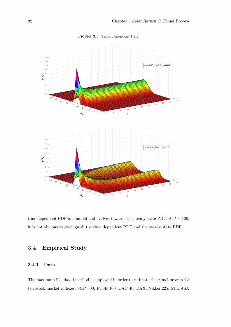
92 Chapter 3 Asset Return & Camel Process
Figure 3.5: Time Dependent PDF
10090
8070
6050
4030
t
2010
0-1-0.8
-0.6-0.4
Xt
-0.20
0.20.4
0.60.8
4
2
6
5
8
3
9
1
0
7
1
p(X
t,t)
α=-0.05; β=0.2; γ=0.05
10090
8070
6050
4030
t
2010
0-1-0.8
-0.6-0.4
Xt
-0.20
0.20.4
0.60.8
7
6
5
4
3
2
1
0
8
1
p(X
t,t)
α=0.05; β=0.2; γ=0.05
time dependent PDF is bimodal and evolves towards the steady state PDF. At t = 100,
it is not obvious to distinguish the time dependent PDF and the steady state PDF.
3.4 Empirical Study
3.4.1 Data
The maximum likelihood method is employed in order to estimate the camel process for
ten stock market indexes, S&P 500, FTSE 100, CAC 40, DAX, Nikkei 225, STI, ASX
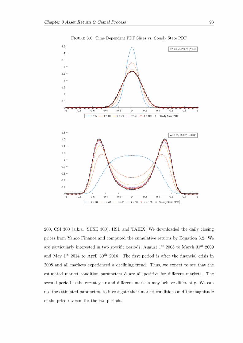
Chapter 3 Asset Return & Camel Process 93
Figure 3.6: Time Dependent PDF Slices vs. Steady State PDF
-1 -0.8 -0.6 -0.4 -0.2 0 0.2 0.4 0.6 0.8 10
0.5
1
1.5
2
2.5
3
3.5
4
4.5
t = 5 t = 10 t = 20 t = 50 t = 100 Steady State PDF
α=-0.05; β=0.2; γ=0.05
-1 -0.8 -0.6 -0.4 -0.2 0 0.2 0.4 0.6 0.8 10
0.2
0.4
0.6
0.8
1
1.2
1.4
1.6
1.8
t = 20 t = 40 t = 60 t = 80 t = 100 Steady State PDF
α=0.05; β=0.2; γ=0.05
200, CSI 300 (a.k.a. SHSE 300), HSI, and TAIEX. We downloaded the daily closing
prices from Yahoo Finance and computed the cumulative returns by Equation 3.2. We
are particularly interested in two specific periods, August 1st 2008 to March 31st 2009
and May 1st 2014 to April 30th 2016. The first period is after the financial crisis in
2008 and all markets experienced a declining trend. Thus, we expect to see that the
estimated market condition parameters α are all positive for different markets. The
second period is the recent year and different markets may behave differently. We can
use the estimated parameters to investigate their market conditions and the magnitude
of the price reversal for the two periods.
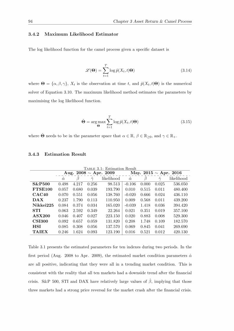
94 Chapter 3 Asset Return & Camel Process
3.4.2 Maximum Likelihood Estimator
The log likelihood function for the camel process given a specific dataset is
L (Θ) =T∑t=1
log p(Xt, t|Θ) (3.14)
where Θ = {α, β, γ}, Xt is the observation at time t, and p(Xt, t|Θ) is the numerical
solver of Equation 3.10. The maximum likelihood method estimates the parameters by
maximising the log likelihood function.
Θ = arg maxΘ
T∑t=1
log p(Xt, t|Θ) (3.15)
where Θ needs to be in the parameter space that α ∈ R, β ∈ R≥0, and γ ∈ R+.
3.4.3 Estimation Result
Table 3.1: Estimation ResultAug. 2008 ∼ Apr. 2009 May. 2015 ∼ Apr. 2016
α β γ likelihood α β γ likelihood
S&P500 0.498 4.217 0.256 98.513 -0.106 0.000 0.025 536.050FTSE100 0.057 0.680 0.039 193.790 0.010 0.515 0.011 480.400CAC40 0.070 0.551 0.056 138.760 -0.020 0.666 0.024 436.110DAX 0.237 1.790 0.113 110.950 0.009 0.568 0.011 439.200Nikkei225 0.084 0.374 0.034 165.020 -0.039 1.418 0.036 394.420STI 0.063 2.592 0.349 22.264 0.021 0.351 0.019 357.100ASX200 0.046 0.407 0.027 223.150 0.020 0.883 0.008 529.300CSI300 0.092 0.657 0.059 131.820 0.208 1.748 0.109 182.570HSI 0.085 0.308 0.056 137.570 0.069 0.845 0.041 269.690TAIEX 0.246 1.624 0.093 123.190 0.016 0.521 0.012 420.130
Table 3.1 presents the estimated parameters for ten indexes during two periods. In the
first period (Aug. 2008 to Apr. 2009), the estimated market condition parameters α
are all positive, indicating that they were all in a trending market condition. This is
consistent with the reality that all ten markets had a downside trend after the financial
crisis. S&P 500, STI and DAX have relatively large values of β, implying that those
three markets had a strong price reversal for the market crash after the financial crisis.
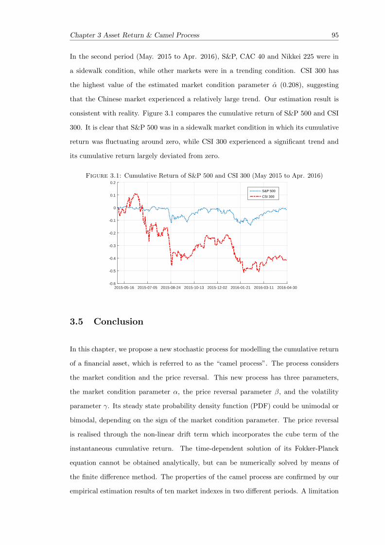
Chapter 3 Asset Return & Camel Process 95
In the second period (May. 2015 to Apr. 2016), S&P, CAC 40 and Nikkei 225 were in
a sidewalk condition, while other markets were in a trending condition. CSI 300 has
the highest value of the estimated market condition parameter α (0.208), suggesting
that the Chinese market experienced a relatively large trend. Our estimation result is
consistent with reality. Figure 3.1 compares the cumulative return of S&P 500 and CSI
300. It is clear that S&P 500 was in a sidewalk market condition in which its cumulative
return was fluctuating around zero, while CSI 300 experienced a significant trend and
its cumulative return largely deviated from zero.
Figure 3.1: Cumulative Return of S&P 500 and CSI 300 (May 2015 to Apr. 2016)
2015-05-16 2015-07-05 2015-08-24 2015-10-13 2015-12-02 2016-01-21 2016-03-11 2016-04-30-0.6
-0.5
-0.4
-0.3
-0.2
-0.1
0
0.1
0.2
S&P 500
CSI 300
3.5 Conclusion
In this chapter, we propose a new stochastic process for modelling the cumulative return
of a financial asset, which is referred to as the “camel process”. The process considers
the market condition and the price reversal. This new process has three parameters,
the market condition parameter α, the price reversal parameter β, and the volatility
parameter γ. Its steady state probability density function (PDF) could be unimodal or
bimodal, depending on the sign of the market condition parameter. The price reversal
is realised through the non-linear drift term which incorporates the cube term of the
instantaneous cumulative return. The time-dependent solution of its Fokker-Planck
equation cannot be obtained analytically, but can be numerically solved by means of
the finite difference method. The properties of the camel process are confirmed by our
empirical estimation results of ten market indexes in two different periods. A limitation

96 Chapter 3 Asset Return & Camel Process
of this chapter is that the parameters of the camel process are possibly time-varying. In
other words, the parameters may not be stable during the two periods in the empirical
analysis. Future research may wish to develop the change point detection for the camel
process.

Appendix
3.A Steady State Solution of the Fokker-Planck Equation
Theorem 3.2 (Fokker-Planck equation). Consider the Ito process Xt with drift µ(Xt)
and volatility σ(Xt), and hence satisfying the SDE dXt = µ(xt)dt + σ(xt)dWt. The
probability density function (PDF) of the ensemble of realisations p(Xt, t) satisfies the
Fokker-Planck equation 8.
∂p(Xt, t)
∂t= − ∂
∂Xt[µ(Xt)p(Xt, t)] +
∂2
∂X2t
[1
2σ(Xt)
2p(Xt, t)
]
The camel process solves the SDE
dXt = (αXt − βX3t )dt+ γdWt, X0 = 0 (3.16)
where α ∈ R, β ∈ R≥0, and γ ∈ R+. The drift term is αXt − βX3t and the volatility
term is γ.
The Fokker-Planck equation for the camel process is
∂p(Xt, t)
∂t= − ∂
∂Xt
[(αXt − βX3
t )p(Xt, t)]
+∂2
∂X2t
[1
2γ2p(Xt, t)
](3.17)
8The Fokker-Planck equation is also known as the Kolmogorov forward equation.
97

98 Chapter 3 Asset Return & Camel Process
By setting ∂p(Xt,t)∂t = 0, we can obtain the steady state PDF p(X) which satisfies the
time-independent Fokker-Planck equation
0 = − ∂
∂X
[(αX − βX3)p(X)
]+
∂2
∂X2
[1
2γ2p(X)
](3.18)
One integral with respect to X
∫0 dX =
∫− ∂
∂X
[(αX − βX3)p(X)
]+
∂2
∂X2
[1
2γ2p(X)
]dX
0 = −(αX − βX3)p(X) +∂
∂X
[1
2γ2p(X)
]+ constant
constant = −(αX − βX3)p(X) +∂
∂X
[1
2γ2p(X)
]
This constant must be zero, as p(X) and its derivatives have to vanish for a large enough
X.
0 = −(αX − βX3)p(X) +∂
∂X
[1
2γ2p(X)
]0 = −(αX − βX3)p(X) +
1
2γ2 dp(X)
dX1
2γ2 dp(X)
dX= (αX − βX3)p(X)
1
p(X)dp(X) =
2(αX − βX3)
γ2dX
Integral on both hand sides
∫1
p(X)dp(X) =
∫2(αX − βX3)
γ2dX
log p(X) =
∫2αX
γ2− 2βX3
γ2dX
=
∫2αX
γ2dX −
∫2βX3
γ2dX
=αX2
γ2− βX4/2
γ2+ constant
=αX2 − βX4/2
γ2+ constant
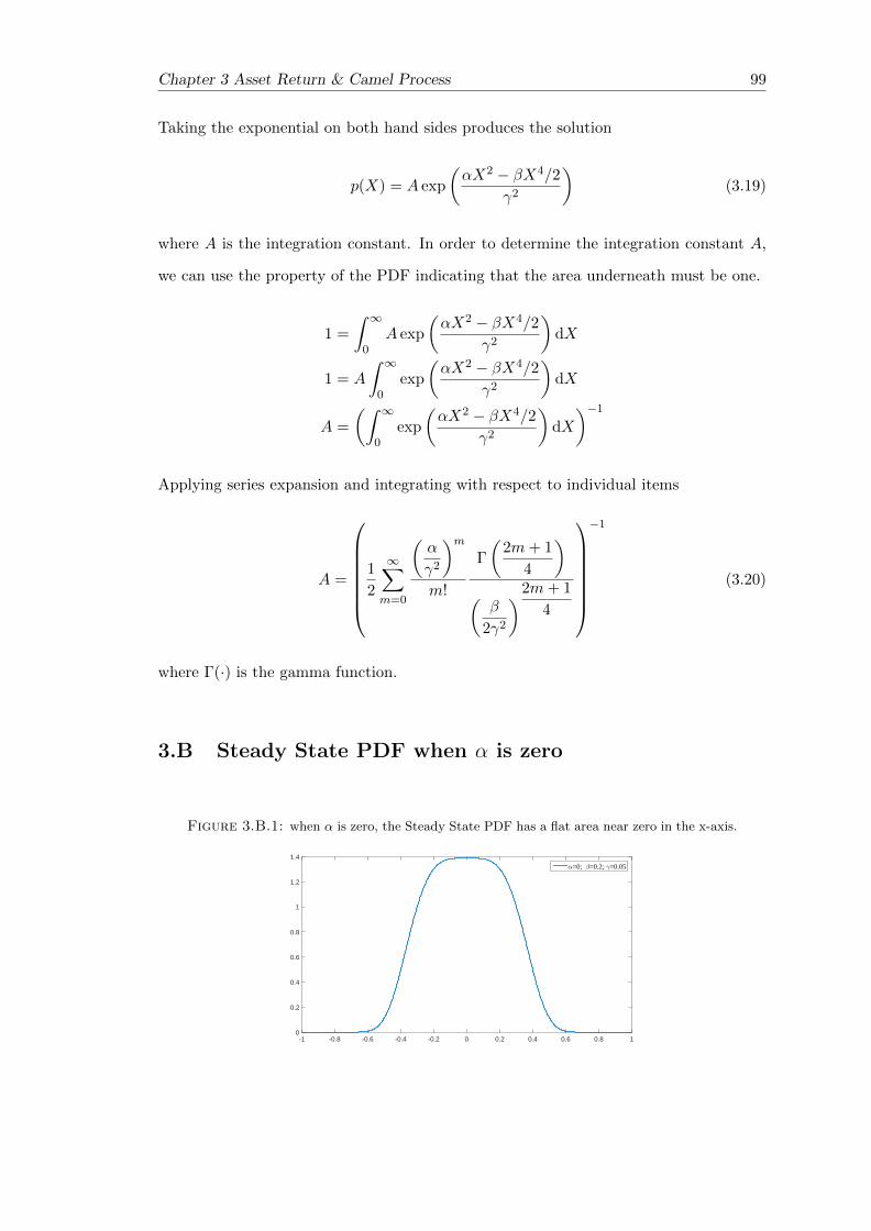
Chapter 3 Asset Return & Camel Process 99
Taking the exponential on both hand sides produces the solution
p(X) = A exp
(αX2 − βX4/2
γ2
)(3.19)
where A is the integration constant. In order to determine the integration constant A,
we can use the property of the PDF indicating that the area underneath must be one.
1 =
∫ ∞0
A exp
(αX2 − βX4/2
γ2
)dX
1 = A
∫ ∞0
exp
(αX2 − βX4/2
γ2
)dX
A =
(∫ ∞0
exp
(αX2 − βX4/2
γ2
)dX
)−1
Applying series expansion and integrating with respect to individual items
A =
1
2
∞∑m=0
(α
γ2
)mm!
Γ
(2m+ 1
4
)(β
2γ2
)2m+ 1
4
−1
(3.20)
where Γ(·) is the gamma function.
3.B Steady State PDF when α is zero
Figure 3.B.1: when α is zero, the Steady State PDF has a flat area near zero in the x-axis.
-1 -0.8 -0.6 -0.4 -0.2 0 0.2 0.4 0.6 0.8 10
0.2
0.4
0.6
0.8
1
1.2
1.4
α=0; β=0.2; γ=0.05

Chapter 4
Forecasting the Log Return of Term Structure for
Chinese Commodity Futures:
an h-step Functional Autoregressive Model
This chapter takes the tools in functional data analysis to understand the term struc-
ture of Chinese commodity futures and forecast their log returns at both short and long
horizons. A functional ANOVA (FANOVA) has been applied in order to examine the
calendar effect of the term structure. We use an h-step Functional Autoregressive model
to forecast the log return of the term structure. Compared with the naive predictor, the
in-sample and out-of-sample forecasting performance indicates that additional forecast-
ing power is gained by using the functional autoregressive structure. Although the log
return at short horizons is not predictable, the forecasts appear to be more accurate at
long horizons due to the stronger temporal dependence. The predictive factor method
has a better in-sample fitting, but it cannot outperform the estimated kernel method for
out-of-sample testing, except in the case of 1-quarter-ahead forecasting.
101

102 Chapter 4 Forecasting the Log Return of Term Structure
4.1 Introduction
As a matter of fact, investors cannot short sell stocks in the Chinese stock market. The
stringent constraints on short selling stocks make it very difficult to manage the downside
risk. Although the index futures contracts were launched by the China Financial Futures
Exchange in 2010, there are many restrictions on the trading of index futures at the
moment. Investors in China are seeking opportunities to broaden the scope of their
portfolio to diversify risk. Many studies have shown that investing in commodity futures
is an effect way to diversify against falling stock prices (e.g. Edwards & Caglayan, 2001;
Jensen et al., 2002; Wang & Yu, 2004; Erb & Harvey, 2006). Gorton & Rouwenhorst
(2006) show that the commodity futures returns are negatively correlated with equity
returns. Ten years later, Bhardwaj et al. (2015) find that their conclusions largely hold
up out-of-sample, and conclude that the negative correlation between commodity futures
returns and equity returns is robust. It is worthwhile and meaningful to investigate the
commodity futures market in China.
The existing literature mainly focuses on forecasting the term structure of government
bond yields. Only a limited number of studies have been devoted to forecasting the term
structure of commodity futures. It is even more difficult to find studies on forecasting
the term structure of commodity futures in developing countries. This chapter fills the
literature gap in the forecasting research on the log return of the term structure for
commodity futures, with a particular interest in Chinese markets, since China has the
largest trading volume of commodity futures in the world.
In 2015, the total trading volume and the trading value of Chinese commodity futures
accounted for 3.237 billion contracts and RMB 136.47 trillion, respectively (Shanghai
Institute of Futures and Derivatives, 2016). Table 4.1 lists the top 10 global futures and
options exchange in 2015 by the trading volume of the commodity futures and options.
Three Chinese commodity futures exchanges, namely the Dalian Commodity Exchange,
Zhengzhou Commodity Exchange, and Shanghai Futures Exchange, were ranked among
the top 3 largest exchanges. Hence, China plays a vital role in the global futures market,
especially for commodity futures.
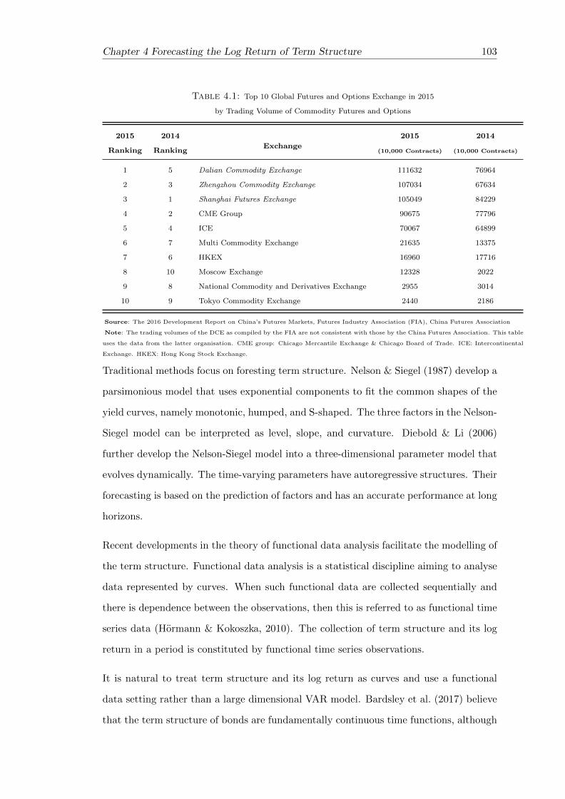
Chapter 4 Forecasting the Log Return of Term Structure 103
Table 4.1: Top 10 Global Futures and Options Exchange in 2015
by Trading Volume of Commodity Futures and Options
2015 2014
Exchange
2015 2014
Ranking Ranking (10,000 Contracts) (10,000 Contracts)
1 5 Dalian Commodity Exchange 111632 76964
2 3 Zhengzhou Commodity Exchange 107034 67634
3 1 Shanghai Futures Exchange 105049 84229
4 2 CME Group 90675 77796
5 4 ICE 70067 64899
6 7 Multi Commodity Exchange 21635 13375
7 6 HKEX 16960 17716
8 10 Moscow Exchange 12328 2022
9 8 National Commodity and Derivatives Exchange 2955 3014
10 9 Tokyo Commodity Exchange 2440 2186
Source: The 2016 Development Report on China’s Futures Markets, Futures Industry Association (FIA), China Futures Association
Note: The trading volumes of the DCE as compiled by the FIA are not consistent with those by the China Futures Association. This table
uses the data from the latter organisation. CME group: Chicago Mercantile Exchange & Chicago Board of Trade. ICE: Intercontinental
Exchange. HKEX: Hong Kong Stock Exchange.
Traditional methods focus on foresting term structure. Nelson & Siegel (1987) develop a
parsimonious model that uses exponential components to fit the common shapes of the
yield curves, namely monotonic, humped, and S-shaped. The three factors in the Nelson-
Siegel model can be interpreted as level, slope, and curvature. Diebold & Li (2006)
further develop the Nelson-Siegel model into a three-dimensional parameter model that
evolves dynamically. The time-varying parameters have autoregressive structures. Their
forecasting is based on the prediction of factors and has an accurate performance at long
horizons.
Recent developments in the theory of functional data analysis facilitate the modelling of
the term structure. Functional data analysis is a statistical discipline aiming to analyse
data represented by curves. When such functional data are collected sequentially and
there is dependence between the observations, then this is referred to as functional time
series data (Hormann & Kokoszka, 2010). The collection of term structure and its log
return in a period is constituted by functional time series observations.
It is natural to treat term structure and its log return as curves and use a functional
data setting rather than a large dimensional VAR model. Bardsley et al. (2017) believe
that the term structure of bonds are fundamentally continuous time functions, although

104 Chapter 4 Forecasting the Log Return of Term Structure
the data are observed only at discrete times. It should be highlighted that the term
structure of commodity futures Pn(t) and its log return are also always existing for all
t, even if we have observations only for some t, i.e. there is a price of a commodity
with delivery t times later after the contract is signed on day n. Pn(t) is a continuous
function in nature.
Bosq (2000) developed the theory of general functional linear processes, including the
functional autoregressive processes, in the Hilbert and Banach spaces. Ramsay & Sil-
verman (2006), Hormann & Kokoszka (2010), and Horvath & Kokoszka (2012) provide
recent theoretical developments in terms of functional linear processes. The conventional
method to estimate the functional autoregressive model is the estimated kernel method
using functional principal components. Kargin & Onatski (2008) develop a more refined
approach by using predictive factors which focus on the directions more relevant to the
predictions. They provide an example using their approach in order to predict the term
structure of the Eurodollar futures rates. Didericksen et al. (2012) study the finite sam-
ple performance of both the estimated kernel method and the predictive factor method,
and their simulation shows that the predictive factor method does not dominate the
estimated kernel method.
In the illustrative example of Kargin & Onatski (2008), they firstly demean the data,
make the prediction for the demeaned data, and then add the mean back for the real
prediction. We believe that it is more natural to forecast the log return of the term
structure by means of the functional AR(1) model. There are two advantages of working
with the log return of the term structure, rather than with the term structure. First,
the log return has zero mean, which can be fed into the functional AR(1) model directly.
Second, the log return of the term structure is usually stationary, which meets the
conditions of the functional AR(1) model. Since we are working with the log return of
the term structure, it is inappropriate to compare our method with traditional methods
(e.g. Diebold & Li, 2006). Following Didericksen et al. (2012), we use a naive predictor
as our benchmark model.
Chapter 4 Forecasting the Log Return of Term Structure 105
The remainder of the chapter is as follows. Section 4.2 describes our data and provides
the functional descriptive statistics. Section 4.3 applies the functional ANOVA in or-
der to examine the calendar effect. Section 4.4 briefly introduces the two prediction
approaches, namely the estimated kernel method and the predictive factor method. In
Section 4.5, the forecasting performance is presented with in-depth discussions. Section
4.6 summarises the chapter.
4.2 Data and Functional Descriptive Statistics
Based on two criteria, we select 18 commodity futures traded in China. First, we
exclude illiquid commodity futures, such as Wire Rod (symbol: WR), Wheat (symbol:
WH), and Early Rice (symbol: RI). Secondly, we exclude commodity futures with too
many missing data. Glass (symbol: FG), Methanol (symbol: MA), and Polypropylene
(symbol: PP) are not considered because of too many missing data. Table 4.1 shows
comprehensive information about the selected commodity futures. Note that the number
of observations for the curve is not exactly the same. For instance, there are 8 points in
the term structure of A, 12 points in that of AG, and 5 points in that of C. It should
be highlighted that this is the reason why a standard multivariate technique cannot be
used.
We use the daily settlement price for the commodity futures that we downloaded from
Wind. Note that different commodity futures have different periods of data. The in-
sample period for training data is from the first date to the middle point of the entire
period, and the out-of-sample period for testing data is from one trading day after the
in-sample period to the end of the entire period. The number of observations in the
in-sample period and the out-of-sample period is approximately the same.
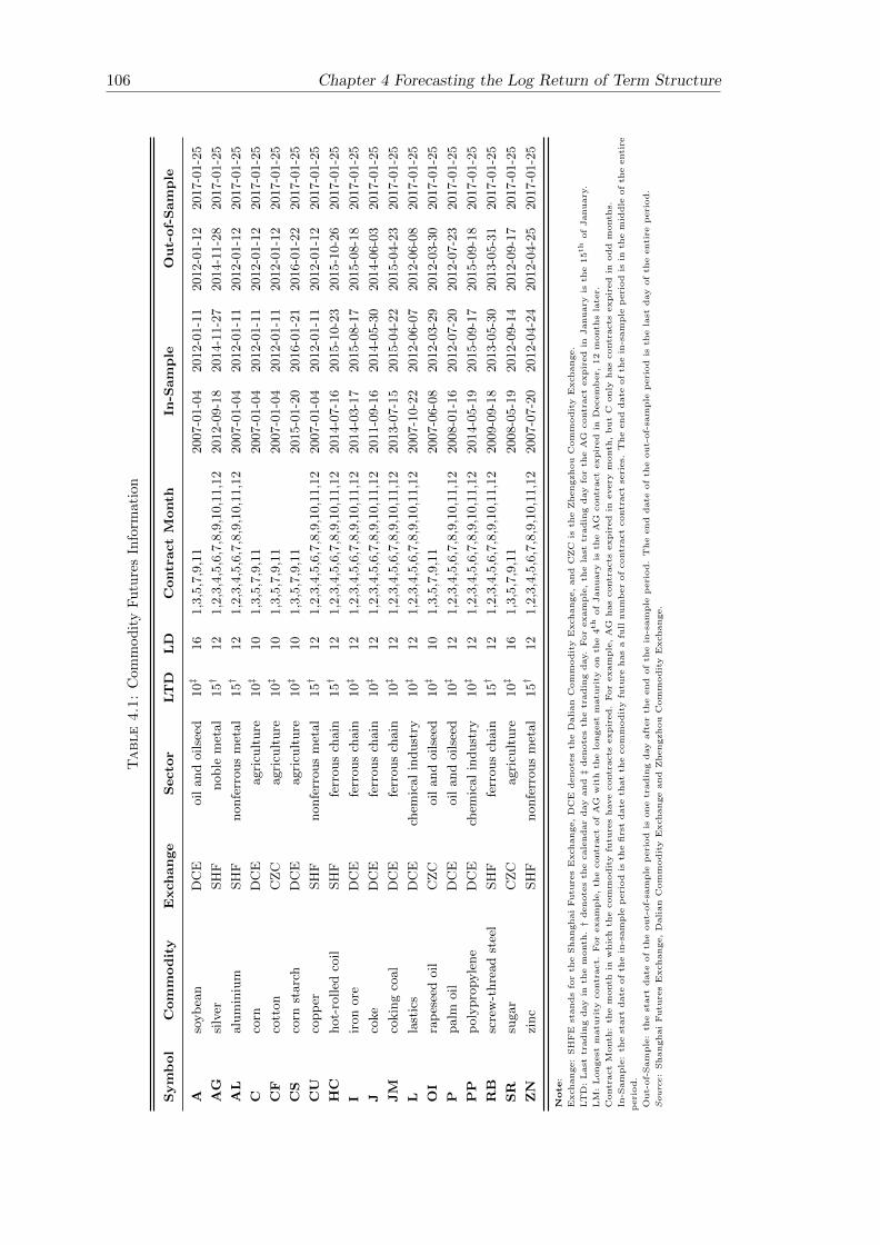
106 Chapter 4 Forecasting the Log Return of Term Structure
Table4.1:
Com
mod
ity
Fu
ture
sIn
form
atio
n
Symbol
Commodity
Exch
ange
Secto
rLTD
LD
ContractM
onth
In-S
ample
Out-of-Sample
Aso
yb
ean
DC
Eoil
and
oilse
ed10‡
16
1,3
,5,7
,9,1
12007-0
1-0
42012-0
1-1
12012-0
1-1
22017-0
1-2
5
AG
silv
erSH
Fnoble
met
al
15†
12
1,2
,3,4
,5,6
,7,8
,9,1
0,1
1,1
22012-0
9-1
82014-1
1-2
72014-1
1-2
82017-0
1-2
5
AL
alu
min
ium
SH
Fnonfe
rrous
met
al
15†
12
1,2
,3,4
,5,6
,7,8
,9,1
0,1
1,1
22007-0
1-0
42012-0
1-1
12012-0
1-1
22017-0
1-2
5
Cco
rnD
CE
agri
cult
ure
10‡
10
1,3
,5,7
,9,1
12007-0
1-0
42012-0
1-1
12012-0
1-1
22017-0
1-2
5
CF
cott
on
CZ
Cagri
cult
ure
10‡
10
1,3
,5,7
,9,1
12007-0
1-0
42012-0
1-1
12012-0
1-1
22017-0
1-2
5
CS
corn
starc
hD
CE
agri
cult
ure
10‡
10
1,3
,5,7
,9,1
12015-0
1-2
02016-0
1-2
12016-0
1-2
22017-0
1-2
5
CU
copp
erSH
Fnonfe
rrous
met
al
15†
12
1,2
,3,4
,5,6
,7,8
,9,1
0,1
1,1
22007-0
1-0
42012-0
1-1
12012-0
1-1
22017-0
1-2
5
HC
hot-
rolled
coil
SH
Ffe
rrous
chain
15†
12
1,2
,3,4
,5,6
,7,8
,9,1
0,1
1,1
22014-0
7-1
62015-1
0-2
32015-1
0-2
62017-0
1-2
5
Iir
on
ore
DC
Efe
rrous
chain
10‡
12
1,2
,3,4
,5,6
,7,8
,9,1
0,1
1,1
22014-0
3-1
72015-0
8-1
72015-0
8-1
82017-0
1-2
5
Jco
ke
DC
Efe
rrous
chain
10‡
12
1,2
,3,4
,5,6
,7,8
,9,1
0,1
1,1
22011-0
9-1
62014-0
5-3
02014-0
6-0
32017-0
1-2
5
JM
cokin
gco
al
DC
Efe
rrous
chain
10‡
12
1,2
,3,4
,5,6
,7,8
,9,1
0,1
1,1
22013-0
7-1
52015-0
4-2
22015-0
4-2
32017-0
1-2
5
Lla
stic
sD
CE
chem
ical
indust
ry10‡
12
1,2
,3,4
,5,6
,7,8
,9,1
0,1
1,1
22007-1
0-2
22012-0
6-0
72012-0
6-0
82017-0
1-2
5
OI
rap
esee
doil
CZ
Coil
and
oilse
ed10‡
10
1,3
,5,7
,9,1
12007-0
6-0
82012-0
3-2
92012-0
3-3
02017-0
1-2
5
Ppalm
oil
DC
Eoil
and
oilse
ed10‡
12
1,2
,3,4
,5,6
,7,8
,9,1
0,1
1,1
22008-0
1-1
62012-0
7-2
02012-0
7-2
32017-0
1-2
5
PP
poly
pro
pyle
ne
DC
Ech
emic
al
indust
ry10‡
12
1,2
,3,4
,5,6
,7,8
,9,1
0,1
1,1
22014-0
5-1
92015-0
9-1
72015-0
9-1
82017-0
1-2
5
RB
scre
w-t
hre
ad
stee
lSH
Ffe
rrous
chain
15†
12
1,2
,3,4
,5,6
,7,8
,9,1
0,1
1,1
22009-0
9-1
82013-0
5-3
02013-0
5-3
12017-0
1-2
5
SR
sugar
CZ
Cagri
cult
ure
10‡
16
1,3
,5,7
,9,1
12008-0
5-1
92012-0
9-1
42012-0
9-1
72017-0
1-2
5
ZN
zinc
SH
Fnonfe
rrous
met
al
15†
12
1,2
,3,4
,5,6
,7,8
,9,1
0,1
1,1
22007-0
7-2
02012-0
4-2
42012-0
4-2
52017-0
1-2
5
Note:
Exchange:
SH
FE
stands
for
the
Shanghai
Futu
res
Exchange,
DC
Edenote
sth
eD
ali
an
Com
modit
yE
xchange,
and
CZ
Cis
the
Zhengzhou
Com
modit
yE
xchange.
LT
D:
Last
tradin
gday
inth
em
onth
.†
denote
sth
ecale
ndar
day
and‡
denote
sth
etr
adin
gday.
For
exam
ple
,th
ela
sttr
adin
gday
for
the
AG
contr
act
expir
ed
inJanuary
isth
e15th
of
January
.
LM
:L
ongest
matu
rity
contr
act.
For
exam
ple
,th
econtr
act
of
AG
wit
hth
elo
ngest
matu
rity
on
the
4th
of
January
isth
eA
Gcontr
act
expir
ed
inD
ecem
ber,
12
month
sla
ter.
Contr
act
Month
:th
em
onth
inw
hic
hth
ecom
modit
yfu
ture
shave
contr
acts
expir
ed.
For
exam
ple
,A
Ghas
contr
acts
expir
ed
inevery
month
,but
Conly
has
contr
acts
expir
ed
inodd
month
s.
In-S
am
ple
:th
est
art
date
of
the
in-s
am
ple
peri
od
isth
efi
rst
date
that
the
com
modit
yfu
ture
has
afu
llnum
ber
of
contr
act
contr
act
seri
es.
The
end
date
of
the
in-s
am
ple
peri
od
isin
the
mid
dle
of
the
enti
re
peri
od.
Out-
of-
Sam
ple
:th
est
art
date
of
the
out-
of-
sam
ple
peri
od
isone
tradin
gday
aft
er
the
end
of
the
in-s
am
ple
peri
od.
The
end
date
of
the
out-
of-
sam
ple
peri
od
isth
ela
stday
of
the
enti
rep
eri
od.
Source:
Shanghai
Futu
res
Exchange,
Dali
an
Com
modit
yE
xchange
and
Zhengzhou
Com
modit
yE
xchange.
Chapter 4 Forecasting the Log Return of Term Structure 107
4.2.1 Term Structure
On each trading day, the term structure is assembled by the price of the contract serials
with the most recent expired contract in the beginning, and the contract expired at the
longest maturity in the end. The rolling of the commodity futures is right after the last
trading day of the month. For example, the term structure of AG on 2016-01-04 was
the sequence of the AG futures contract expired in January 2016, February 2016, up to
December 2016. On 2016-01-18, the term structure of AG became the contract serials
expired in February 2016, March 2016, up to January 2017. We will use the functional
ANOVA in order to examine the calendar effect of the term structure.
4.2.2 Log Return of the Term Structure
Instead of forecasting the term structure, we choose to forecast the log return of the
term structure at various horizons (i.e. different h-steps), which is defined in Equation
4.1.
Xn(t) = [log(Pn(t))− log(Pn−h(t))] ∗ 100, where h ∈ {1, 5, 20, 60} (4.1)
where t is the time to maturity, and Pn(t) is the term structure at date n.
There are two advantages of working with the log return of the term structure, rather
than with the term structure. First, the log return has zero mean, which can be fed into
the functional AR(1) model directly. There is no need to demean the data. Second, the
functional observations need to be stationary in order to be modelled by the functional
AR(1) model. Analogical to the scalar case, the asset price is typically deemed as a
non-stationary process, while the log return of the asset price tends to be stationary.
Intuitively, the term structure is highly likely to be non-stationary, while the log return
would be stationary. We confirm the stationarity of the log returns by checking the
existence condition ‖Ψh‖2 < 1. Other recent developed tests, such as the functional
stationarity test (Horvath et al., 2014; Aue & Van Delft, 2017), can be used as well.

108 Chapter 4 Forecasting the Log Return of Term Structure
Regarding forecasting horizons, we select four h-steps, including 1, 5, 20, 60. When
h = 1, Xn(t) is the daily log return of the term structure, and Xn+1(t) is the 1-day-
ahead forecast. When h = 5, Xn(t) is the weekly log return of the term structure, and
Xn+5(t) is the 1-week-ahead forecast. When h = 20, Xn(t) is the monthly log return of
the term structure, and Xn+20(t) is the 1-month-ahead forecast. When h = 60, Xn(t)
is the quarterly log return of the term structure, and Xn+1(t) is the 1-quarter-ahead
forecast. Longer forecasting horizons could be considered, but due to the availability
of data, we cap the forecasting horizon at 60 trading days. Figure 4.1 shows the term
structure for Steel Rebar (symbol: RB). Figure 4.2 presents the log return of the term
structure at four horizons.
Figure 4.1: Term Structure (RB)
1500
12
2000
2500
10
3000
2017
3500
8 2016
4000
2015
4500
62014
5000
5500
4 2013
20122
2011
20100
Figure 4.2: Log Return of the Term Structure (RB)

Chapter 4 Forecasting the Log Return of Term Structure 109
4.2.3 Functional Descriptive Statistics
Following Ramsay & Silverman (2006, Chapter 2), we provide basic functional descrip-
tive statistics, including the functional mean, functional standard deviation, and func-
tional correlation, for both the term structure and the log return of the term structure.
Functional Mean & Functional Standard Deviation
Figure 4.3 shows the sample functional mean and the sample standard deviation of the
term structure for 18 commodity futures. Unlike the upside sloping term structure of
the government bond yields studied in (Diebold & Li, 2006), the mean curves of the
commodity futures term structure are relatively flat. The possible explanation could be
that the longest maturity is only 12 months ahead, which is much shorter than that of
the term structure of bond yields (120 months). The term structure of all 18 commodity
futures has a large standard deviation in our sample period. For the term structure, it
is not obvious to observe how the standard deviation varies with the time to maturity.
Figure 4.4 shows the sample functional mean and the sample standard deviation of the
log returns of the term structure. The functional means of the log return are very close
to a zero function. This fact enables us to use the functional AR(1) model for the log
return directly without the demean procedure. The functional standard deviation of the
log return increases with h. AL has the smallest magnitude of the functional standard
deviation. The commodity futures in the sector of ferrous chain (e.g. HC, I, and J) tend
to have a large functional standard deviation.
There are three patterns of the relationship between the functional standard deviation
and the time to maturity. The first pattern is that the standard deviation is negatively
related to the time to maturity. In other words, the standard deviation is larger when
the time to maturity is short. Most commodity futures belong to the first pattern. The
second pattern is the positive relationship between the standard deviation and the time
to maturity. The example is CU, in which the standard deviation increases after six
months of the time to maturity. The third pattern is that the standard deviation is flat,
not related to the time to maturity. AG, AL, and ZN are classified into this pattern.
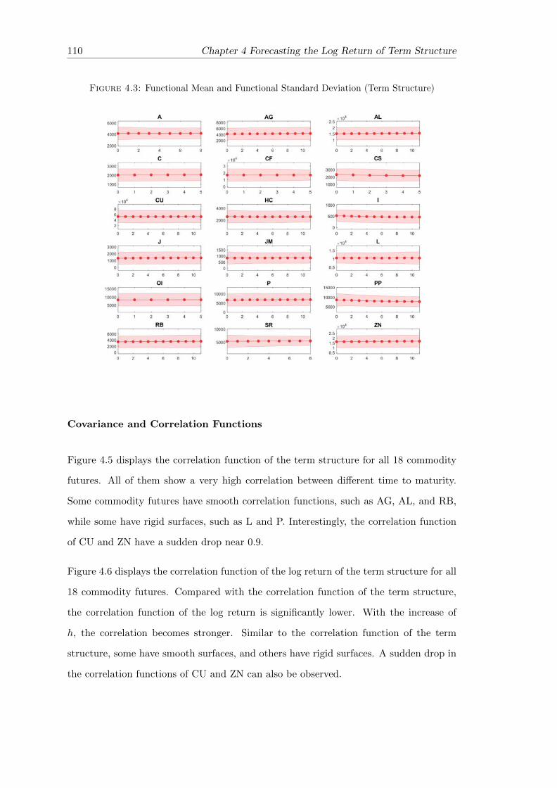
110 Chapter 4 Forecasting the Log Return of Term Structure
Figure 4.3: Functional Mean and Functional Standard Deviation (Term Structure)
Covariance and Correlation Functions
Figure 4.5 displays the correlation function of the term structure for all 18 commodity
futures. All of them show a very high correlation between different time to maturity.
Some commodity futures have smooth correlation functions, such as AG, AL, and RB,
while some have rigid surfaces, such as L and P. Interestingly, the correlation function
of CU and ZN have a sudden drop near 0.9.
Figure 4.6 displays the correlation function of the log return of the term structure for all
18 commodity futures. Compared with the correlation function of the term structure,
the correlation function of the log return is significantly lower. With the increase of
h, the correlation becomes stronger. Similar to the correlation function of the term
structure, some have smooth surfaces, and others have rigid surfaces. A sudden drop in
the correlation functions of CU and ZN can also be observed.

Chapter 4 Forecasting the Log Return of Term Structure 111
Figure 4.4: Functional Mean and Functional Standard Deviation (Log Return of theTerm Structure)
(a) Daily Log Return (b) Weekly Log Return
(c) Monthly Log Return (d) Quarterly Log Return

112 Chapter 4 Forecasting the Log Return of Term Structure
Figure 4.5: Correlation Functions (Term Structure)
0.61
0.8
1
A
0.5
1
0.50 0
0.9961
0.998
1
AG
0.5
1
0.50 0
0.961
0.98
1
AL
0.5
1
0.50 0
0.81
0.9
1
C
0.5
1
0.50 0
0.951 1
CF
0.5
1
0.50 0
0.91
0.95
1
CS
0.5
1
0.50 0
0.961
0.98
1
CU
0.5
1
0.50 0
0.91
0.95
1
HC
0.5
1
0.50 0
0.91
0.95
1
I
0.5
1
0.50 0
0.81
0.9
1
J
0.5
1
0.50 0
0.81
0.9
1
JM
0.5
1
0.50 0
0.61
0.8
1
L
0.5
1
0.50 0
0.951 1
OI
0.5
1
0.50 0
0.91
0.95
1
P
0.5
1
0.50 0
0.91
0.95
1
PP
0.5
1
0.50 0
0.961
0.98
1
RB
0.5
1
0.50 0
0.91
0.95
1
SR
0.5
1
0.50 0
0.961
0.98
1
ZN
0.5
1
0.50 0
4.3 FANOVA
We employ the one-way functional ANOVA (FANOVA) developed by Horvath & Rice
(2015) to examine the season of the year effect (SoY), month of the year effect (MoY),
week of the month effect (WoM), and day of the week effect (DoW). It is inappropriate
to apply the FANOVA on the log return of the term structure because they all tend to
have mean zero functions.
The test has the null hypothesis H0 that the mean curves of multiple functional popu-
lations are the same vs. the alternative HA that H0 does not hold.
H0 : µ1(·) = µ2(·) = ... = µk(·)
HA : H0 does not hold

Chapter 4 Forecasting the Log Return of Term Structure 113
Figure 4.6: Correlation Functions (Log Return of the Term Structure)
01
0.5
1
A
0.5
1
0.50 0
0.81
0.9
1
AG
0.5
1
0.50 0
01
0.5
1
AL
0.5
1
0.50 0
01
0.5
1
C
0.5
1
0.50 0
1
0.6
1
0.8
CF
0.5
1
0.50 0
01
0.5
1
CS
0.5
1
0.50 0
01
0.5
1
CU
0.5
1
0.50 0
01
0.5
1
HC
0.5
1
0.50 0
01
0.5
1
I
0.5
1
0.50 0
01
0.5
1
J
0.5
1
0.50 0
-11
0
1
JM
0.5
1
0.50 0
-11
0
1
L
0.5
1
0.50 0
01
0.5
1
OI
0.5
1
0.50 0
-11
0
1
P
0.5
1
0.50 0
01
0.5
1
PP
0.5
1
0.50 0
01
0.5
1
RB
0.5
1
0.50 0
1
0.6
1
0.8
SR
0.5
1
0.50 0
1
0.6
1
0.8
ZN
0.5
1
0.50 0
(a) Daily Log Return
01
0.5
1
A
0.5
1
0.50 0
0.951 1
AG
0.5
1
0.50 0
1
0.6
1
0.8
AL
0.5
1
0.50 0
01
0.5
1
C
0.5
1
0.50 0
0.61
0.8
1
CF
0.5
1
0.50 0
01
0.5
1
CS
0.5
1
0.50 0
01
0.5
1
CU
0.5
1
0.50 0
01
0.5
1
HC
0.5
1
0.50 0
01
0.5
1
I
0.5
1
0.50 0
01
0.5
1
J
0.5
1
0.50 0
01
0.5
1
JM
0.5
1
0.50 0
-11
0
1
L
0.5
1
0.50 0
01
0.5
1
OI
0.5
1
0.50 0
01
0.5
1
P
0.5
1
0.50 0
01
0.5
1
PP
0.5
1
0.50 0
1
0.6
1
0.8
RB
0.5
1
0.50 0
0.61
0.8
1
SR
0.5
1
0.50 0
0.61
0.8
1
ZN
0.5
1
0.50 0
(b) Weekly Log Return
1
0.6
1
0.8
A
0.5
1
0.50 0
0.961
0.98
1
AG
0.5
1
0.50 0
0.61
0.8
1
AL
0.5
1
0.50 0
01
0.5
1
C
0.5
1
0.50 0
0.61
0.8
1
CF
0.5
1
0.50 0
01
0.5
1
CS
0.5
1
0.50 0
01
0.5
1
CU
0.5
1
0.50 0
0.61
0.8
1
HC
0.5
1
0.50 0
01
0.5
1
I
0.5
1
0.50 0
1
0.6
1
0.8
J
0.5
1
0.50 0
01
0.5
1
JM
0.5
1
0.50 0
01
0.5
1
L
0.5
1
0.50 0
0.61
0.8
1
OI
0.5
1
0.50 0
01
0.5
1
P
0.5
1
0.50 0
0.61
0.8
1
PP
0.5
1
0.50 0
0.61
0.8
1
RB
0.5
1
0.50 0
0.61
0.8
1
SR
0.5
1
0.50 0
0.81
0.9
1
ZN
0.5
1
0.50 0
(c) Monthly Log Return
0.61
0.8
1
A
0.5
1
0.50 0
0.981
0.99
1
AG
0.5
1
0.50 0
0.81
0.9
1
AL
0.5
1
0.50 0
01
0.5
1
C
0.5
1
0.50 0
0.81
0.9
1
CF
0.5
1
0.50 0
1
0.6
1
0.8
CS
0.5
1
0.50 0
0.61
0.8
1
CU
0.5
1
0.50 0
0.61
0.8
1
HC
0.5
1
0.50 0
0.61
0.8
1
I
0.5
1
0.50 0
0.61
0.8
1
J
0.5
1
0.50 0
0.61
0.8
1
JM
0.5
1
0.50 0
01
0.5
1
L
0.5
1
0.50 0
0.81
0.9
1
OI
0.5
1
0.50 0
0.61
0.8
1
P
0.5
1
0.50 0
0.61
0.8
1
PP
0.5
1
0.50 0
0.61
0.8
1
RB
0.5
1
0.50 0
0.61
0.8
1
SR
0.5
1
0.50 0
0.91
0.95
1
ZN
0.5
1
0.50 0
(d) Quarterly Log Return
114 Chapter 4 Forecasting the Log Return of Term Structure
The core idea of the test is to calculate the empirical score vectors by using the eigen-
functions associated with the d largest eigenvalues of DN,p or DN defined as
λϕi(t) =
∫DN (t, s)ϕi(s)ds (4.2)
Then the statistics TN1 can be calculated.
TN =k∑i=1
Ni
(ξi· − ξ··
)TΣ−1i
(ξi· − ξ··
)(4.3)
where
Σi =
{∫ ∫DNi,i(t, s)ϕl(t)ϕj(s)dtdt, 1 ≤ j, l ≤ d
}(4.4)
ξ·· =
(k∑i=1
NiΣi−1
)−1 k∑i=1
NiΣi−1ξi· (4.5)
ξi· =1
Ni
Ni∑i=1
Ni∑i=1
ξij (4.6)
ξij = (〈Xi,j , ϕ1〉, 〈Xi,j , ϕ2〉, ..., 〈Xi,j , ϕd〉)T (4.7)
The test statistics TN has the following limit distribution under the null hypothesis.
TND−→ χ2(d(k − 1))
where χ2(d(k− 1)) denotes a χ2 random variable with d(k− 1) degrees of freedom. k is
the number of functional populations, and d is the number of the basis for the projection.
The number d is determined by the rule that approximately ν% of the sample variance
is explained by the first d principal components. We choose ν% = 95% in this study.
Following Horvath & Rice (2015), we also use the flat top kernel to estimate the long-run
1There is another version of the statistics TN . Interested readers can refer to Horvath & Rice (2015).

Chapter 4 Forecasting the Log Return of Term Structure 115
covariance kernel, which is shown in Equation 4.8. nan
K(x) =
1, if 0 ≤ t < 1
1.1− |t|, if 0.1 ≤ t < 1.1
0, if |t| ≥ 1.1
(4.8)
with the bandwidth parameter equal to N1/4.
Our data sample can be divided into different population groups according to four cal-
endar criteria, which are the season of the year (SoY) 2, month of the year (MoY), week
of the month (WoM), and day of the week (DoW). The FANOVA is applied to test
whether the mean curves in different populations are the same. If the test is rejected,
then there could be a market anomaly of the calendar effect.
Since the term structure from different years but the same season/month could have
different means just according to the difference in those years, it is necessary to firstly
demean the data in each year before the functional AVONA is applied to test the SoY/-
MoY. Similarly, the data is demeaned in each month for testing the WoM and the data
is demeaned in each week for testing the DoW.
Table 4.1 reports the test statistics and their p-values. Concerning the SoY and MoY,
the test of most commodity futures is strongly rejected. There are significant SoY and
MoY for most commodity futures. We use JM as a representative example. Figure 4.1
shows the mean curves (demeaned for each year) of the JM term structure for each season
and each month. It is apparent that the mean curve of JM in winter is downside sloping,
while others are upside sloping. The mean curves of JM in different months show the
same pattern with downside sloping curves in November, December, and January. The
calendar effect of JM could be explained by the energy consumption in China. JM is
one of the main sources of heat in northern China. The demand of JM is typically high
in winter. It becomes straightforward that the price of JM in winter is higher, which
causes the downside sloping term structure of JM in winter.
2The four seasons in China are defined as follows. Spring: February, March, April; Summer: May,June, July; Fall: August, September, October; Winter: November, December, January.

116 Chapter 4 Forecasting the Log Return of Term Structure
It is reasonable to observe no SoY in HC and ZN. HC is the raw material for the
production of automobiles, vessels, and so forth. The main usage of ZN is in order to
produce anti-corrosion zinc coating, zinc-base alloy, and zinc oxide, which is commonly
utilised in the later stage of the production processes for automobiles, vessels, and light
industries. There is no obvious SoY for those industries.
It is expected to observe the SoY in agricultural commodity futures. Interestingly, the
FANOVA shows no SoY for SR, while the MoY is very significant for SR. Figure 4.2
shows the mean curves (demeaned for each year) of the SR term structure. The SR
term structure in winter seems to be higher than in other seasons, but the FANOVA
shows that the difference is not significant. The reason can be explained as follows. It
can be observed in Figure 4.3(b) that the SR has a relatively lower term structure in
January and comparatively a higher term structure in November and December. Since
the spring in China consists of January, November, and December, the mean curve of
SR in spring is mixed by relatively high and low curves, which forces it to be closer to
the global mean and further makes the SoY of SR insignificant.
Regarding the WoM, there is very strong evidence for RB, strong evidence for AL, I, PP,
ZN, and weak evidence for CS and JM. Figure 4.4(a) displays the mean curves (demeaned
for each month). Note that the last trading day for the contract of RB expired in the
current month is the 15th calendar day in a month. Before the last trading day, the
mean curves of Week 1 and 2 are both upside sloping. After the last trading day, the
mean curves of Week 3 and 4 are both downside sloping.
In terms of the DoW, the test shows that Al and SR are rejected at the 1% significance
level; CF, CS, J, P, and RB are rejected at the 5% significance level; and OI, PP, and
ZN are rejected at the 10 % significance level. Taking RB as an example, Figure 4.4(b)
depicts the mean curves of the RB term structure (demeaned for each week). The
differences among the first four weekdays are not obvious, but the term structure in
Friday is clearly relatively lower than the others. This anomaly of lower term structure
on Friday can be explained by the investment behaviour. The commodity future of
RB in China is a highly volatile investment asset. Some investors in China avoid to
take risks during the weekend. They choose to clear their holding positions on Friday

Chapter 4 Forecasting the Log Return of Term Structure 117
and establish the position again on next Monday. Therefore the RB term structure is
abnormally lower than the other weekdays.
Table 4.1: FANOVA Results
SoY P-value MoY P-value WoM P-value DoW P-value
A 59.213∗∗∗ (0.00) 95.399∗∗∗ (0.00) 9.127 (0.87) 24.937 (0.41)
AG 13.252∗∗∗ (0.00) 53.755∗∗∗ (0.00) 5.179 (0.16) 5.254 (0.26)
AL 13.087∗∗∗ (0.00) 39.187∗∗∗ (0.00) 14.077∗∗ (0.03) 29.589∗∗∗ (0.00)
C 88.965∗∗∗ (0.00) 194.717∗∗∗ (0.00) 17.386 (0.30) 20.072 (0.45)
CF 8.150∗∗ (0.04) 13.994 (0.23) 6.934 (0.64) 22.134∗∗ (0.04)
CS 137.703∗∗∗ (0.00) 399.862∗∗∗ (0.00) 23.769∗ (0.07) 33.036∗∗ (0.03)
CU 8.918∗∗ (0.03) 23.675∗∗ (0.01) 13.402 (0.15) 11.589 (0.48)
HC 0.861 (0.83) 9.435 (0.58) 15.916 (0.60) 36.878 (0.25)
I 15.971∗∗∗ (0.00) 32.730∗∗∗ (0.00) 18.431∗∗ (0.03) 19.184 (0.74)
J 72.615∗∗∗ (0.00) 216.472∗∗∗ (0.00) 24.016 (0.46) 55.637∗∗ (0.02)
JM 11.319∗∗ (0.01) 23.421∗∗ (0.02) 23.742∗ (0.07) 30.254 (0.35)
L 28.755∗∗∗ (0.00) 88.203∗∗∗ (0.00) 31.407 (0.25) 31.538 (0.68)
OI 26.519∗∗∗ (0.00) 46.965∗∗∗ (0.00) 10.419 (0.32) 26.101∗ (0.05)
P 33.163∗∗∗ (0.00) 75.643∗∗∗ (0.00) 28.270 (0.25) 58.122∗∗ (0.01)
PP 27.572∗∗∗ (0.00) 51.428∗∗∗ (0.00) 31.794∗∗ (0.02) 45.835∗ (0.05)
RB 50.549∗∗∗ (0.00) 110.470∗∗∗ (0.00) 23.117∗∗∗ (0.00) 27.393∗∗ (0.01)
SR 4.438 (0.22) 27.823∗∗∗ (0.00) 6.237 (0.72) 35.512∗∗∗ (0.00)
ZN 2.939 (0.40) 9.349 (0.59) 13.320∗∗ (0.04) 19.471∗ (0.08)
Note: SoY: Season of the Year; MoY: Month of the Year; WoM: Week of the Month; DoW: Day of the WeekFor testing the SoY and MoY, the data is demeaned for each year. For testing the WoM, the data is demeaned for
each month. For testing the DoW, the data is demeaned for each week.***p < 0.01, **p < 0.05, *p < 0.1
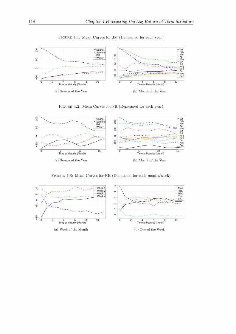
118 Chapter 4 Forecasting the Log Return of Term Structure
Figure 4.1: Mean Curves for JM (Demeaned for each year)
0 2 4 6 8 10
−5
00
50
10
0
Time to Maturity (Month)
SpringSummerFallWinter
(a) Season of the Year
0 2 4 6 8 10
−5
00
50
10
0
Time to Maturity (Month)
JanFebMarAprMayJunJulAugSepOctNovDec
(b) Month of the Year
Figure 4.2: Mean Curves for SR (Demeaned for each year)
0 5 10 15
−5
00
50
10
0
Time to Maturity (Month)
SpringSummerFallWinter
(a) Season of the Year
0 5 10 15
−1
00
01
00
20
0
Time to Maturity (Month)
JanFebMarAprMayJunJulAugSepOctNovDec
(b) Month of the Year
Figure 4.3: Mean Curves for RB (Demeaned for each month/week)
0 2 4 6 8 10−1
5−
50
51
0
Time to Maturity (Month)
Week 1Week 2Week 3Week 4
(a) Week of the Month
0 2 4 6 8 10
−4
−2
02
46
Time to Maturity (Month)
Mon.Tue.Wed.Thu.Fri.
(b) Day of the Week
Chapter 4 Forecasting the Log Return of Term Structure 119
4.4 h-step Functional Autoregressive Model
Bosq (2000) developed the theory of general functional linear processes, including the
functional autoregressive process, in the Hilbert and Banach spaces. Ramsay & Silver-
man (2006), Hormann & Kokoszka (2010), and Horvath & Kokoszka (2012) provide re-
cent theoretical developments in functional linear processes. All functions in the Hilbert
space L2 are real square integrable functions on the interval [0, 1] with inner product
〈f, g〉 =∫f(t)g(t)dt. Recall the definition of the functional AR(1) model.
Xn(t) = Ψ(Xn−1(t)) + εn (4.9)
where {Xn(t),−∞ < n <∞} is a sequence of mean zero functional observations in the
Hilbert space L2, {εn,−∞ < n <∞} is a sequence of the i.i.d. mean zero functional
errors also in L2, satisfying E‖εn‖2 < ∞, and Ψ ∈ L is a linear operator mapping a
curve into another curve. Here we propose an h-step functional AR(1) model defined in
a similar way.
Xn(t) = Ψh(Xn−h(t)) + εn (4.10)
where h is the forecasting horizon, and Ψh ∈ L is also a linear operator. The operator
Ψh is defined as
Ψh(X(t)) =
∫ψh(t, s)X(s)dt (4.11)
where ψ(t, s) is a bivariate kernel.
There are two versions of the existence condition for the functional AR(1) model. The
weak version is proved by Horvath & Kokoszka (2012), and the strong version is provided
by Didericksen et al. (2012). If condition C0 or C1 holds, then there is a unique strictly
stationary causal solution to Equation 4.9.
C0 (weak version): There exists an integer j0 such that ‖Ψj0h ‖ < 1.
C1 (strong version): ‖Ψh‖ < 1, where ‖Ψh‖2 =∫ ∫
ψh(t, s)2dtds.
Note that condition C0 is more general than condition C1. Practically, the condition
C1 is more convenient to use.
120 Chapter 4 Forecasting the Log Return of Term Structure
In this chapter, we employ two prediction methods for the functional AR(1) model under
finite sample. The first method is the estimated kernel, which uses only a few of the
most important empirical functional principle components (EFPC) to estimate kernel
ψ(t, s). The second method is the predictive factor, developed by Kargin & Onatski
(2008). The key idea of the second method is to replace the EFPCs by directions which
are the most relevant for predictions.
4.4.1 Estimated Kernel
Analogical to the scalar AR(1) model, the most intuitive estimator for Ψh would be
Ψh = ChC−1, where the functional covariance C and lag-h autocovariance Ch operator
are defined by
C(x) = E [〈Xn, x〉Xn] , x ∈ L2 (4.12)
Ch(x) = E [〈Xn, x〉Xn+h] , x ∈ L2 (4.13)
The empirical covariance and empirical lag-h autocovariance operator can be estimated
by
C(x) =1
N
N∑j=1
〈Xi, x〉Xj+1 (4.14)
Ch(x) =1
N − h
N−h∑k=1
〈Xi, x〉Xk+h (4.15)
Horvath & Kokoszka (2012) show that the inverse of the covariance operator C is not
bounded. In order to avoid working with the reciprocals of very small eigenvalues, it is
sensible to use only the first p most important EFPC. Practically, the number of p can
be determined by several methods, including the cumulative variance method, cross-
validation, and information criteria. Denote the EFPC of the functional observations
Xn as, νj , j = 1, 2, 3..., p, the inverse of covariance operator using the first p EFPCs can
be defined as
Γp(x) =
p∑j=1
λ−1j 〈x, νj〉 νj (4.16)
Chapter 4 Forecasting the Log Return of Term Structure 121
Then we can obtain the estimator for Ψh,p
Ψh,p = ChΓp(x) (4.17)
= Ch
p∑j=1
λ−1j 〈x, νj〉 νj
(4.18)
=1
N − h
N−h∑k=1
⟨Xk,
p∑j=1
λ−1j 〈x, νj〉 νj
⟩Xk+h (4.19)
=1
N − h
N−h∑k=1
p∑j=1
λ−1j 〈x, νj〉 〈Xk, νj〉Xk+h (4.20)
If a smoothing procedure is applied on Xk+h ≈∑p
i=1 〈Xk+h, νi〉 νi, the estimator further
becomes
Ψh,p =1
N − h
N−h∑k=1
p∑j=1
p∑i=1
λ−1j 〈x, νj〉 〈Xk, νj〉 〈Xk+h, νi〉 νi (4.21)
The estimated kernel for the estimator in Equation 4.21 is
ψh,p(t, s) =1
N − h
N−h∑k=1
p∑j=1
p∑i=1
λ−1j 〈Xk, νj〉 〈Xk+h, νi〉 νj(s)νi(t) (4.22)
Using the estimated kernel, we can make h-step predictions as
Xn+h(t) =
∫ψh,pXn(s)ds (4.23)
=
p∑j=1
(p∑i=1
ψh,p 〈Xn, νi〉
)νj(t) (4.24)
4.4.2 Predictive Factors
Kargin & Onatski (2008) develop the predictive factor decomposition for the estima-
tion of the functional autoregression operator, which is a dimension-reduction technique
aiming to minimise the prediction error. This method is different from the estimated ker-
nel method, which is based on the functional principle analysis, because it is designed
to identify the directions (linear combinations of components) that are most relevant
for prediction rather than describing variance. Here we briefly explain the regularised
version of the method for the h-step prediction.
122 Chapter 4 Forecasting the Log Return of Term Structure
The method aims to find an operator A which can minimise the prediction error
min{E‖Xn+h −A(Xn)‖2; A ∈ Rk
}(4.25)
where Rk is the set of all rank k operators mapping L2 into a subspace of dimension k.
In order to solve this problem, Kargin & Onatski (2008) employ the polar decomposition
of ΨC1/2
ΨC1/2 = UΦ1/2, Φ = C1/2ΨTΨC1/2 (4.26)
Then the optimisation problem becomes
E‖Xn+h −Ψh,k(Xn)‖2 (4.27)
where Ψh,k is defined as
Ψh,k(y) =k∑i=1
σ−1i
⟨y,ΨTΨC1/2(xi)
⟩U(xi) (4.28)
where σ21 > ... > σ2
k > 0 are the largest k eigenvalues of Φ. The operation in Equation
4.28 is equivalent to
Ψh,k(y) =
k∑i=1
〈y, bi〉Ch(bi), bi = C−1/2(xi) (4.29)
where the processes {〈y, bi〉 , i = 1, ..., k)} are named as the predictive factors, and the
functions {Ch(bi), i = 1, ..., k)} are named as the corresponding predictive loadings, which
are the most relevant “directions” in L2 for prediction.
Since C−1/2 is also not a bounded estimator, Kargin & Onatski (2008) proposed the
following regularised version for consistent estimation.
Φα,h = C−1/2α CTh ChC
−1/2α , Cα = C + αI (4.30)
Chapter 4 Forecasting the Log Return of Term Structure 123
where α ∈ R+ is a regularisation parameter and I is the identity operator. Then the
h-step prediction can be made by
Xn+h(t) = Ψα,h,k(Xn(t))
=
k∑i=1
⟨Xn(t), bα,i
⟩Ch(bα,i), bα,i = C−1/2
α (xα,i)(4.31)
where σ2α,1 > ... > σ2
α,k are the largest k eigenvalues of Φα,h, and xα,1, ..., xα,k are the
corresponding eigenfunctions.
In practice, we need to select the value of the regularisation parameter α. In this study,
we use a numerical optimiser to choose α which minimises the total prediction error in
the in-sample period data.
4.4.3 Forecast Performance Evaluation
For the sake of measuring the overall forecasting performance in a period, we propose
to use the functional RMSE (FRMSE)
FRMSE =
√√√√ 1
N
N∑i=1
(∫ 1
0
(Xi(t)− Xi(t)
)2dt
)(4.32)
In order to compare forecasting performance among different commodities, we developed
the functional R2. Since the functional AR(1) sequence has a zero mean, we define the
functional total sum of squares (FTSS) for a functional observation as
FTSS =N∑i=1
(∫ 1
0Xi(t)
2dt
)(4.33)
The functional residual sum of squares (FRSS) is defined as
FRSS =N∑i=1
(∫ 1
0
(Xi(t)− Xi(t)
)2dt
)(4.34)
124 Chapter 4 Forecasting the Log Return of Term Structure
The functional R2 (FR2) is defined as
FR2 =FTSS − FRSS
FTSS(4.35)
4.5 Forecasting Performance
Traditional methods (e.g. Diebold & Li, 2006) focus on foresting the term structure. Our
functional AR(1) model is more suitable to forecast the log return of the term struc-
ture. It is not appropriate to compare our method with traditional methods. Following
Didericksen et al. (2012), we use a naive prediction (NP) method as the benchmark
model. The naive predictor set Xn+h(t) = Xn(t), which does not consider the temporal
dependence. Compared with the naive predictor, we can see the additional forecasting
power gained by using the functional autoregressive structure of the data.
Prior to forecasting, we need to choose the number of EFPCs (p) for the estimated kernel
method, and the number of predictive factors (k) for the predictive factor method. In
order not to use future information, the parameter optimisation is conducted only by
the in-sample period data. We have experimented with the cross-validation procedure,
but the optimised p and k tend to be the maximum number of EFPCs or predictive
factors. Section 4.4.1 has shown the potential danger of working with the reciprocals of
very small eigenvalues. We decide to report the results of {p, k} = 3, 4, 5.
Regarding the values of the regularisation parameter α for the predictive factor method,
we employ a numerical optimiser3 in order to find the optimised value of α that minimises
the forecasting FRMSE in the in-sample period for each commodity futures. Table 4.1
reports the optimised values 4 of α for four forecasting horizons of each commodity
futures. When the forecasting horizon is short, like 1-day-ahead and 1-week-ahead, the
optimised α has very small values. When the forecasting horizon is long, like 1-month-
ahead and 1-week-ahead, the optimised α could be very large for some commodity
futures, such as HC and CS.
3The numerical optimiser used is fminunc in Matlab.4Notice that the values reported in the table are α× 1000
Chapter 4 Forecasting the Log Return of Term Structure 125
The strong existence condition for the functional AR(1) model is that ‖Ψh‖ < 1. In
order to ensure that the model is used in a proper way, we calculate the norm of the
estimated kernel, i.e. ‖Ψh‖. As described in Section 4.4.1, the kernel can be estimated
by only the first p most important EFPCs. In order to avoid redundancy, we only
report the value of ‖Ψh‖ by using the first 5 EFPCs for both the in-sample period and
out-of-sample period.
With the purpose of saving space, we only report the best model FR2. Notice that FR2
could have negative values because of our definition in Equation 4.35. The interpretation
of a negative FR2 would be that the model produces more variation than the FTSS. In
this case, the prediction of a zero function could outperform the model.
4.5.1 In-Sample Fitting
The upper panel of Table 4.2 to Table 4.5 present the in-sample forecasting errors
(FRMSE), ‖Ψh‖, and FR2 for four different forecasting horizons. We will use EK
to denote the estimated kernel method and PF to denote the predictive factors method.
Within the same forecasting horizon, there are three observations about the in-sample
fitting.
• Both the EK and PF method can consistently outperform the naive predictor,
based on the FRMSE. This indicates that additional forecasting power could be
gained by using the functional autoregressive structure.
• Using the same p/k, the PF method has a better fitting than EK. The better
performance of PF could be the idea that PF focuses on the directions that are
most relevant for the prediction, rather than the directions describing variance.
Compared with the EK method, the PF has one additional turning parameter α.
The improved performance may also come from the introduction of an additional
parameter.
• For both EK and PF, the FRMSE is decreasing with more EFPCs or predictive
factors. Using more EFPCs or predictive factors can always give a better fitting
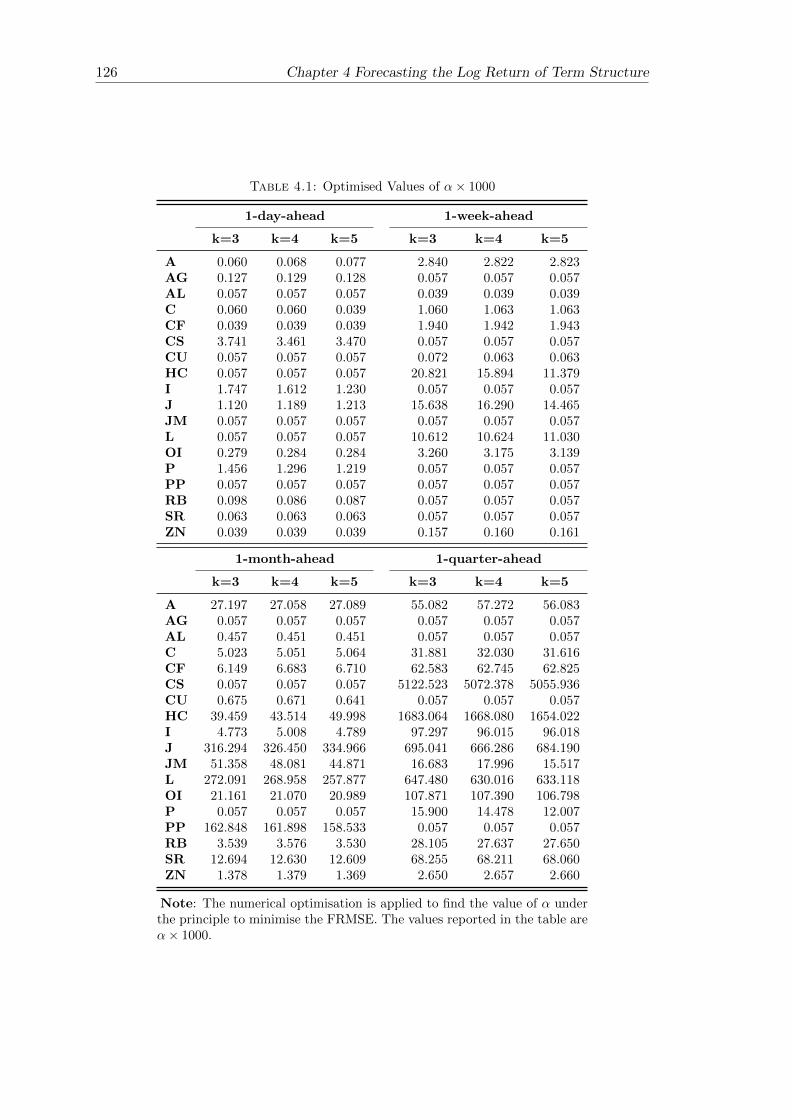
126 Chapter 4 Forecasting the Log Return of Term Structure
Table 4.1: Optimised Values of α× 1000
1-day-ahead 1-week-ahead
k=3 k=4 k=5 k=3 k=4 k=5
A 0.060 0.068 0.077 2.840 2.822 2.823AG 0.127 0.129 0.128 0.057 0.057 0.057AL 0.057 0.057 0.057 0.039 0.039 0.039C 0.060 0.060 0.039 1.060 1.063 1.063CF 0.039 0.039 0.039 1.940 1.942 1.943CS 3.741 3.461 3.470 0.057 0.057 0.057CU 0.057 0.057 0.057 0.072 0.063 0.063HC 0.057 0.057 0.057 20.821 15.894 11.379I 1.747 1.612 1.230 0.057 0.057 0.057J 1.120 1.189 1.213 15.638 16.290 14.465JM 0.057 0.057 0.057 0.057 0.057 0.057L 0.057 0.057 0.057 10.612 10.624 11.030OI 0.279 0.284 0.284 3.260 3.175 3.139P 1.456 1.296 1.219 0.057 0.057 0.057PP 0.057 0.057 0.057 0.057 0.057 0.057RB 0.098 0.086 0.087 0.057 0.057 0.057SR 0.063 0.063 0.063 0.057 0.057 0.057ZN 0.039 0.039 0.039 0.157 0.160 0.161
1-month-ahead 1-quarter-ahead
k=3 k=4 k=5 k=3 k=4 k=5
A 27.197 27.058 27.089 55.082 57.272 56.083AG 0.057 0.057 0.057 0.057 0.057 0.057AL 0.457 0.451 0.451 0.057 0.057 0.057C 5.023 5.051 5.064 31.881 32.030 31.616CF 6.149 6.683 6.710 62.583 62.745 62.825CS 0.057 0.057 0.057 5122.523 5072.378 5055.936CU 0.675 0.671 0.641 0.057 0.057 0.057HC 39.459 43.514 49.998 1683.064 1668.080 1654.022I 4.773 5.008 4.789 97.297 96.015 96.018J 316.294 326.450 334.966 695.041 666.286 684.190JM 51.358 48.081 44.871 16.683 17.996 15.517L 272.091 268.958 257.877 647.480 630.016 633.118OI 21.161 21.070 20.989 107.871 107.390 106.798P 0.057 0.057 0.057 15.900 14.478 12.007PP 162.848 161.898 158.533 0.057 0.057 0.057RB 3.539 3.576 3.530 28.105 27.637 27.650SR 12.694 12.630 12.609 68.255 68.211 68.060ZN 1.378 1.379 1.369 2.650 2.657 2.660
Note: The numerical optimisation is applied to find the value of α underthe principle to minimise the FRMSE. The values reported in the table areα× 1000.
Chapter 4 Forecasting the Log Return of Term Structure 127
for the in-sample period data, but more p/k may overfit the data, as indicated
by the out-of-sample forecasting performance. PF with five predictive factors can
always give the best in-sample fitting.
Across different forecasting horizons, there are four comments about the in-sample fit-
ting.
• With a longer forecasting horizon, the FRMSE becomes larger. This is an intuitive
result because more uncertainty will arise with a longer forecasting horizon. The
quarterly log return has a larger magnitude of variation than the daily log return.
• ‖Ψh‖ are mostly less than 1, expect for the 1-quarter-ahead forecasting of four
commodity futures, namely AG, CF, CS, and OI. The strong existence condition
of the functional AR(1) model is that ‖Ψh‖ < 1. Most log returns of different com-
modity futures at different horizons meet the condition, except that the quarterly
log return of those four commodity futures is larger than 1. This suggests that the
quarterly log return of those four commodity futures could be non-stationary, and
cannot be modelled by the functional AR(1) model.
• With a longer forecasting horizon, ‖Ψh‖ becomes larger. For the 1-day-ahead
and 1-week-ahead forecasting, ‖Ψh‖ is very small, generally less than 0.1. The
temporal dependence of the daily and weekly log return is relatively weak, which
is the reason for the low FR2 of the functional AR(1) model. Hence, the log
returns at short horizons are not predictable. The temporal dependence of the
monthly and quarterly log return becomes stronger, implied by the larger values
of ‖Ψh‖. Thus, the forecasts appear to be more accurate at long horizons due to
the stronger temporal dependence.
• When the forecasting horizon is short, FR2 is normally less than 15%, indicating
a small power of forecasting. With the increase of the forecasting horizon, FR2 is
getting larger. For the 1-month-ahead forecasting, FR2 is around 40% for many
commodities, such as I, L, and P. For the 1-quarter-ahead forecasting, FR2 can
be larger than 50 %, with CF, HC, and I close to 80%.
128 Chapter 4 Forecasting the Log Return of Term Structure
Our results are consistent with Horvath & Kokoszka (2012, Chapter 13) and Didericksen
et al. (2012). Their simulation results show that a larger value of ‖Ψh‖ significantly and
visibly improves the predictions using the functional autoregressive structure.
4.5.2 Out-of-Sample Forecasting
For the out-of-sample forecasting, we recursively estimate the model and use the most
updated parameter to make the next forecast. At date n, the model is firstly estimated
by the data {Xd(t), 1 ≤ d ≤ n}, and then the h-step forecast for Xn+h(t) is conducted by
either the EK or PF method. The optimised α for the PF method is always the same as
the in-sample 5. In this recursively updated manner, we can reduce the potential danger
of over-fitting in the in-sample period since the values of the parameters are updated
with new coming observations.
The lower panels of Table 4.2 to Table 4.5 present the in-sample forecasting errors
(FRMSE), ‖Ψh‖, and FR2 for four different forecasting horizons. There are three ob-
servations about the out-of-sample testing.
• Both EK and PF outperform the naive predictor for the out-of-sample forecasting.
This double-confirm the benefit of using functional autoregressive structure to
forecast the log return of the term structure.
• When the forecasting horizon is short, EK outperforms PF. As for the 1-quarter-
ahead forecasting, PF shows increased predictive power than EK. Similarly to the
in-sample results, the value of ‖Ψh‖ is larger when the forecasting horizon is longer.
It suggests that PF could outperform EK under the condition that the temporal
dependence is strong.
• As can be seen from FR2, the out-of-sample forecasting is less accurate than the
in-sample fitting. There are two possible reasons for a good in-sample fitting but
a bad out-of-sample forecasting. First, the data generation process (DGP) could
be changed. At least the parameter of the DGP could be different. Second, there
could be over-fitting in the in-sample period data. Using more EFPCs or predictive
5We do not choose to update α recursively because of extremely high computational costs.

Chapter 4 Forecasting the Log Return of Term Structure 129
factors does not produce a better forecasting. This also suggests that there could
be overfitting in the in-sample period data. However, we have conducted out-of-
sample forecasting in a recursive way. The parameters are recursively updated.
The danger of overfitting is already mitigated.
It is interesting to see that the log returns at short horizons are not predictable, and
the forecasts appear much accurate at long horizons. Diebold & Li (2006) also find that
their model is more accurate at long horizons. The possible reason could be that the
magnitude of noise at short horizons is relatively larger than the fundamental values of
the term structure and its log returns. Under longer horizons, the relative magnitude
of noise would be smaller, with the comparison to the fundamental values. Then the
temporal dependence becomes stronger, which further enables the functional AR(1)
model to have a better forecast.
4.6 Conclusion
In this chapter, our aim is to forecast the log return of the term structure for Chinese
commodity futures. There are two advantages of working with the log return of the
term structure, rather than with the term structure. First, the log return has zero
mean, which can be fed into the functional AR(1) model directly. Second, the log return
of the term structure is stationary which can be modelled by the functional AR(1).
We start our analysis by inspecting the functional descriptive statistics. Compared
with the term structure of bond yields, the functional mean curves show that the term
structure for Chinese commodity futures is relatively flat. The relationship between the
functional standard deviation and the time to maturity has three patterns, negative,
positive, and not related.
The FANOVA has been applied to examine the calendar effect of the term structure.
SoY and MoY are found in most commodity futures. HC and ZN do not have both SoY
and MoY; CF has SoY but no MoY; while SR has MoY but no SoY. There is very strong
evidence for the WoM on RB. Before the last trading day in the month, the RB term
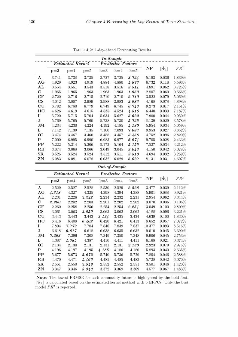
130 Chapter 4 Forecasting the Log Return of Term Structure
Table 4.2: 1-day-ahead Forecasting Results
In-SampleEstimated Kernel Predictive Factors
NP ‖Ψ1‖ FR2
p=3 p=4 p=5 k=3 k=4 k=5
A 3.741 3.738 3.735 3.727 3.725 3.724 5.193 0.036 1.839%AG 4.929 4.923 4.919 4.884 4.880 4.877 6.732 0.118 5.593%AL 3.554 3.551 3.543 3.518 3.516 3.514 4.891 0.062 3.725%C 1.965 1.965 1.963 1.963 1.963 1.963 2.807 0.060 0.666%CF 2.720 2.716 2.715 2.710 2.710 2.710 3.522 0.079 5.069%CS 3.012 3.007 2.989 2.988 2.983 2.983 4.168 0.078 4.898%CU 6.782 6.780 6.779 6.749 6.745 6.743 9.273 0.017 2.151%HC 4.626 4.619 4.615 4.535 4.524 4.516 6.440 0.030 7.187%I 5.720 5.715 5.704 5.634 5.627 5.622 7.900 0.044 9.950%J 5.769 5.765 5.760 5.738 5.730 5.725 8.139 0.029 3.578%JM 4.234 4.230 4.224 4.192 4.185 4.180 5.954 0.034 5.059%L 7.142 7.139 7.135 7.100 7.093 7.087 9.953 0.027 3.852%OI 3.474 3.467 3.460 3.458 3.457 3.456 4.752 0.096 2.820%P 7.000 6.995 6.990 6.983 6.977 6.974 9.705 0.028 2.433%PP 5.222 5.214 5.206 5.173 5.164 5.155 7.527 0.034 3.212%RB 3.074 3.068 3.066 3.049 3.045 3.043 4.150 0.042 5.078%SR 3.525 3.524 3.524 3.512 3.511 3.510 4.694 0.032 3.259%ZN 6.083 6.081 6.078 6.032 6.029 6.027 8.131 0.031 4.607%
Out-of-Sample
Estimated Kernel Predictive FactorsNP ‖Ψ1‖ FR2
p=3 p=4 p=5 k=3 k=4 k=5
A 2.529 2.527 2.528 2.530 2.529 2.526 3.477 0.039 2.112%AG 4.318 4.327 4.325 4.398 4.394 4.388 5.901 0.088 0.921%AL 2.231 2.226 2.222 2.234 2.232 2.231 2.954 0.062 3.344%C 2.200 2.202 2.203 2.201 2.202 2.202 3.070 0.036 0.106%CF 2.260 2.258 2.256 2.254 2.254 2.254 3.049 0.100 2.809%CS 3.061 3.063 3.059 3.063 3.062 3.062 4.188 0.096 3.221%CU 3.443 3.443 3.443 3.434 3.435 3.434 4.639 0.100 1.830%HC 6.416 6.408 6.402 6.420 6.421 6.413 8.652 0.057 7.072%I 7.804 7.779 7.784 7.846 7.839 7.837 10.377 0.093 8.516%J 6.618 6.617 6.618 6.638 6.635 6.632 9.010 0.045 3.390%JM 7.293 7.296 7.308 7.349 7.350 7.348 9.906 0.045 2.753%L 4.387 4.385 4.387 4.410 4.411 4.411 6.168 0.021 0.374%OI 2.134 2.130 2.131 2.131 2.131 2.130 2.923 0.079 2.975%P 4.196 4.197 4.195 4.185 4.186 4.186 5.893 0.040 2.635%PP 5.677 5.673 5.672 5.740 5.736 5.729 7.804 0.046 2.588%RB 4.470 4.471 4.466 4.485 4.485 4.483 5.728 0.042 6.070%SR 2.551 2.550 2.549 2.552 2.552 2.551 3.501 0.046 1.420%ZN 3.347 3.346 3.343 3.372 3.369 3.369 4.577 0.067 1.483%
Note: The lowest FRMSE for each commodity future is highlighted by the bold font.‖Ψ1‖ is calculated based on the estimated kernel method with 5 EFPCs. Only the bestmodel FR2 is reported.
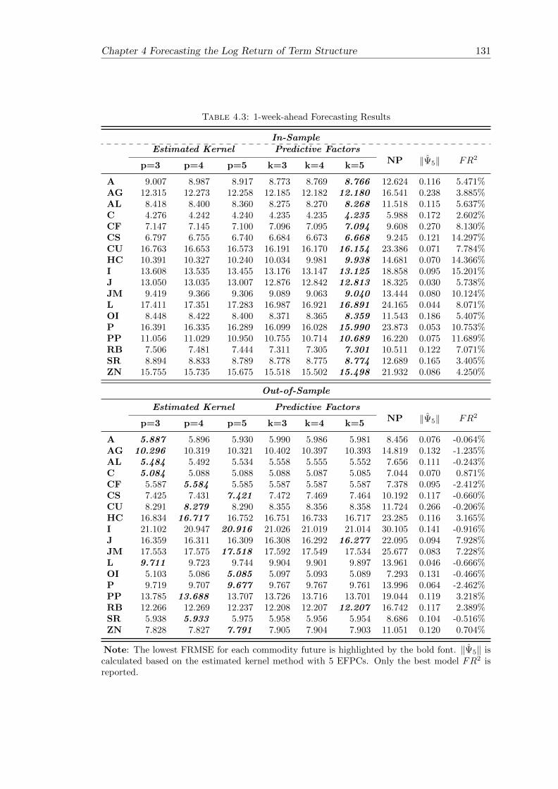
Chapter 4 Forecasting the Log Return of Term Structure 131
Table 4.3: 1-week-ahead Forecasting Results
In-SampleEstimated Kernel Predictive Factors
NP ‖Ψ5‖ FR2
p=3 p=4 p=5 k=3 k=4 k=5
A 9.007 8.987 8.917 8.773 8.769 8.766 12.624 0.116 5.471%AG 12.315 12.273 12.258 12.185 12.182 12.180 16.541 0.238 3.885%AL 8.418 8.400 8.360 8.275 8.270 8.268 11.518 0.115 5.637%C 4.276 4.242 4.240 4.235 4.235 4.235 5.988 0.172 2.602%CF 7.147 7.145 7.100 7.096 7.095 7.094 9.608 0.270 8.130%CS 6.797 6.755 6.740 6.684 6.673 6.668 9.245 0.121 14.297%CU 16.763 16.653 16.573 16.191 16.170 16.154 23.386 0.071 7.784%HC 10.391 10.327 10.240 10.034 9.981 9.938 14.681 0.070 14.366%I 13.608 13.535 13.455 13.176 13.147 13.125 18.858 0.095 15.201%J 13.050 13.035 13.007 12.876 12.842 12.813 18.325 0.030 5.738%JM 9.419 9.366 9.306 9.089 9.063 9.040 13.444 0.080 10.124%L 17.411 17.351 17.283 16.987 16.921 16.891 24.165 0.044 8.071%OI 8.448 8.422 8.400 8.371 8.365 8.359 11.543 0.186 5.407%P 16.391 16.335 16.289 16.099 16.028 15.990 23.873 0.053 10.753%PP 11.056 11.029 10.950 10.755 10.714 10.689 16.220 0.075 11.689%RB 7.506 7.481 7.444 7.311 7.305 7.301 10.511 0.122 7.071%SR 8.894 8.833 8.789 8.778 8.775 8.774 12.689 0.165 3.405%ZN 15.755 15.735 15.675 15.518 15.502 15.498 21.932 0.086 4.250%
Out-of-Sample
Estimated Kernel Predictive FactorsNP ‖Ψ5‖ FR2
p=3 p=4 p=5 k=3 k=4 k=5
A 5.887 5.896 5.930 5.990 5.986 5.981 8.456 0.076 -0.064%AG 10.296 10.319 10.321 10.402 10.397 10.393 14.819 0.132 -1.235%AL 5.484 5.492 5.534 5.558 5.555 5.552 7.656 0.111 -0.243%C 5.084 5.088 5.088 5.088 5.087 5.085 7.044 0.070 0.871%CF 5.587 5.584 5.585 5.587 5.587 5.587 7.378 0.095 -2.412%CS 7.425 7.431 7.421 7.472 7.469 7.464 10.192 0.117 -0.660%CU 8.291 8.279 8.290 8.355 8.356 8.358 11.724 0.266 -0.206%HC 16.834 16.717 16.752 16.751 16.733 16.717 23.285 0.116 3.165%I 21.102 20.947 20.916 21.026 21.019 21.014 30.105 0.141 -0.916%J 16.359 16.311 16.309 16.308 16.292 16.277 22.095 0.094 7.928%JM 17.553 17.575 17.518 17.592 17.549 17.534 25.677 0.083 7.228%L 9.711 9.723 9.744 9.904 9.901 9.897 13.961 0.046 -0.666%OI 5.103 5.086 5.085 5.097 5.093 5.089 7.293 0.131 -0.466%P 9.719 9.707 9.677 9.767 9.767 9.761 13.996 0.064 -2.462%PP 13.785 13.688 13.707 13.726 13.716 13.701 19.044 0.119 3.218%RB 12.266 12.269 12.237 12.208 12.207 12.207 16.742 0.117 2.389%SR 5.938 5.933 5.975 5.958 5.956 5.954 8.686 0.104 -0.516%ZN 7.828 7.827 7.791 7.905 7.904 7.903 11.051 0.120 0.704%
Note: The lowest FRMSE for each commodity future is highlighted by the bold font. ‖Ψ5‖ iscalculated based on the estimated kernel method with 5 EFPCs. Only the best model FR2 isreported.
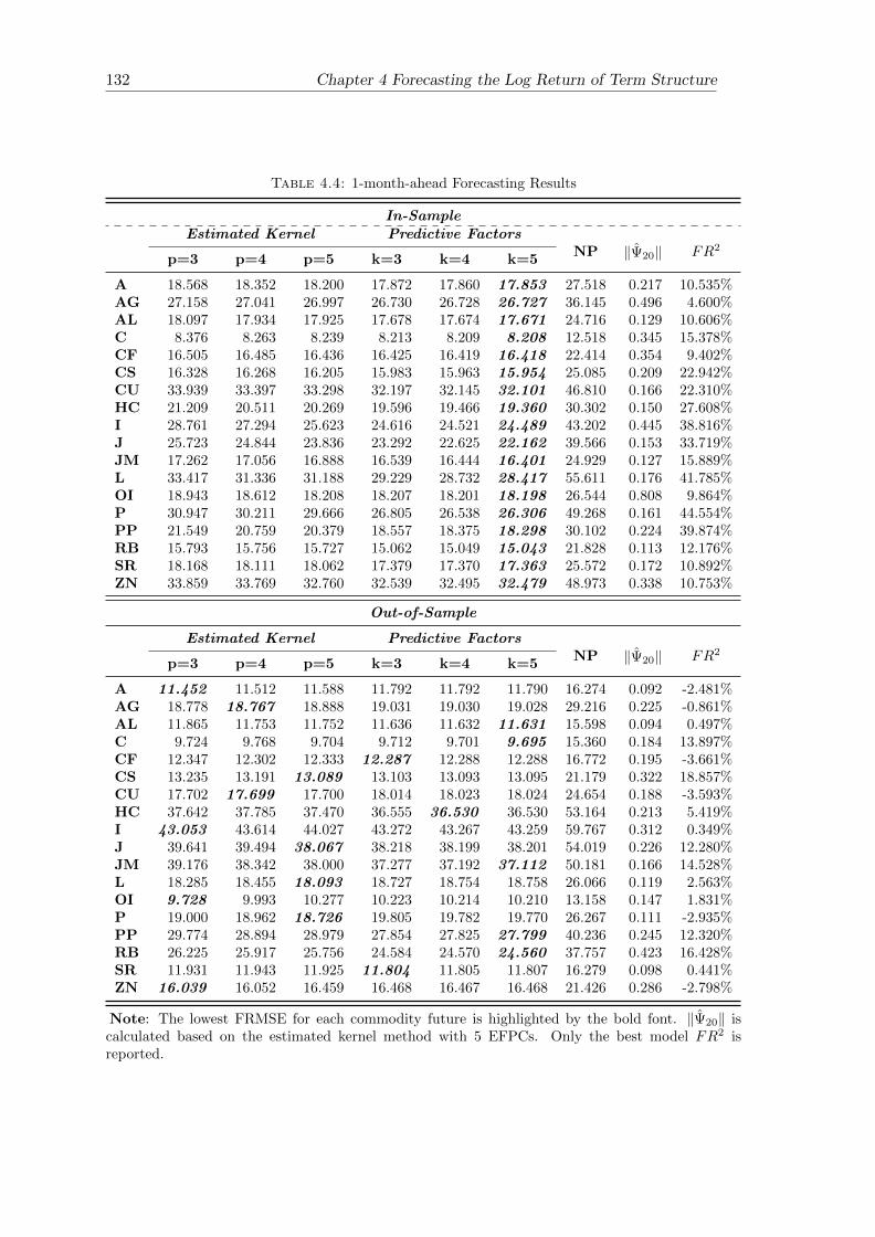
132 Chapter 4 Forecasting the Log Return of Term Structure
Table 4.4: 1-month-ahead Forecasting Results
In-SampleEstimated Kernel Predictive Factors
NP ‖Ψ20‖ FR2
p=3 p=4 p=5 k=3 k=4 k=5
A 18.568 18.352 18.200 17.872 17.860 17.853 27.518 0.217 10.535%AG 27.158 27.041 26.997 26.730 26.728 26.727 36.145 0.496 4.600%AL 18.097 17.934 17.925 17.678 17.674 17.671 24.716 0.129 10.606%C 8.376 8.263 8.239 8.213 8.209 8.208 12.518 0.345 15.378%CF 16.505 16.485 16.436 16.425 16.419 16.418 22.414 0.354 9.402%CS 16.328 16.268 16.205 15.983 15.963 15.954 25.085 0.209 22.942%CU 33.939 33.397 33.298 32.197 32.145 32.101 46.810 0.166 22.310%HC 21.209 20.511 20.269 19.596 19.466 19.360 30.302 0.150 27.608%I 28.761 27.294 25.623 24.616 24.521 24.489 43.202 0.445 38.816%J 25.723 24.844 23.836 23.292 22.625 22.162 39.566 0.153 33.719%JM 17.262 17.056 16.888 16.539 16.444 16.401 24.929 0.127 15.889%L 33.417 31.336 31.188 29.229 28.732 28.417 55.611 0.176 41.785%OI 18.943 18.612 18.208 18.207 18.201 18.198 26.544 0.808 9.864%P 30.947 30.211 29.666 26.805 26.538 26.306 49.268 0.161 44.554%PP 21.549 20.759 20.379 18.557 18.375 18.298 30.102 0.224 39.874%RB 15.793 15.756 15.727 15.062 15.049 15.043 21.828 0.113 12.176%SR 18.168 18.111 18.062 17.379 17.370 17.363 25.572 0.172 10.892%ZN 33.859 33.769 32.760 32.539 32.495 32.479 48.973 0.338 10.753%
Out-of-Sample
Estimated Kernel Predictive FactorsNP ‖Ψ20‖ FR2
p=3 p=4 p=5 k=3 k=4 k=5
A 11.452 11.512 11.588 11.792 11.792 11.790 16.274 0.092 -2.481%AG 18.778 18.767 18.888 19.031 19.030 19.028 29.216 0.225 -0.861%AL 11.865 11.753 11.752 11.636 11.632 11.631 15.598 0.094 0.497%C 9.724 9.768 9.704 9.712 9.701 9.695 15.360 0.184 13.897%CF 12.347 12.302 12.333 12.287 12.288 12.288 16.772 0.195 -3.661%CS 13.235 13.191 13.089 13.103 13.093 13.095 21.179 0.322 18.857%CU 17.702 17.699 17.700 18.014 18.023 18.024 24.654 0.188 -3.593%HC 37.642 37.785 37.470 36.555 36.530 36.530 53.164 0.213 5.419%I 43.053 43.614 44.027 43.272 43.267 43.259 59.767 0.312 0.349%J 39.641 39.494 38.067 38.218 38.199 38.201 54.019 0.226 12.280%JM 39.176 38.342 38.000 37.277 37.192 37.112 50.181 0.166 14.528%L 18.285 18.455 18.093 18.727 18.754 18.758 26.066 0.119 2.563%OI 9.728 9.993 10.277 10.223 10.214 10.210 13.158 0.147 1.831%P 19.000 18.962 18.726 19.805 19.782 19.770 26.267 0.111 -2.935%PP 29.774 28.894 28.979 27.854 27.825 27.799 40.236 0.245 12.320%RB 26.225 25.917 25.756 24.584 24.570 24.560 37.757 0.423 16.428%SR 11.931 11.943 11.925 11.804 11.805 11.807 16.279 0.098 0.441%ZN 16.039 16.052 16.459 16.468 16.467 16.468 21.426 0.286 -2.798%
Note: The lowest FRMSE for each commodity future is highlighted by the bold font. ‖Ψ20‖ iscalculated based on the estimated kernel method with 5 EFPCs. Only the best model FR2 isreported.
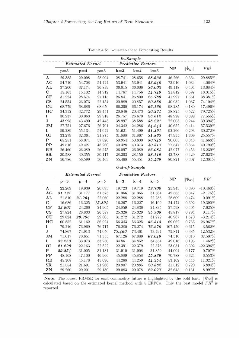
Chapter 4 Forecasting the Log Return of Term Structure 133
Table 4.5: 1-quarter-ahead Forecasting Results
In-SampleEstimated Kernel Predictive Factors
NP ‖Ψ60‖ FR2
p=3 p=4 p=5 k=3 k=4 k=5
A 29.385 29.098 28.904 28.741 28.658 28.632 46.266 0.364 29.885%AG 54.710 54.708 54.424 53.941 53.941 53.940 73.916 1.034 4.064%AL 37.200 37.174 36.839 36.015 36.006 36.002 49.118 0.404 13.684%C 15.163 15.102 14.912 14.767 14.756 14.749 21.812 0.597 18.315%CF 31.224 28.574 27.115 26.841 26.800 26.789 41.997 1.561 38.381%CS 24.554 23.073 22.154 20.989 20.857 20.850 40.932 1.037 74.104%CU 68.779 68.686 68.650 66.200 66.174 66.160 98.285 0.180 17.496%HC 34.352 32.772 29.451 20.846 20.473 20.274 38.825 0.522 79.725%I 30.237 30.063 29.918 26.757 26.670 26.612 48.928 0.399 77.555%J 43.998 43.490 42.443 38.997 38.588 38.221 72.003 0.244 39.394%JM 27.751 27.676 26.701 24.342 24.286 24.243 40.652 0.414 57.539%L 59.289 55.134 54.642 51.621 51.499 51.391 92.266 0.293 30.272%OI 33.279 32.364 31.875 31.888 31.867 31.863 47.955 1.309 25.557%P 65.251 58.074 57.826 50.954 50.830 50.743 90.603 0.343 41.668%PP 49.516 49.427 48.260 40.428 40.373 40.317 77.547 0.354 40.790%RB 26.460 26.289 26.275 26.097 26.089 26.084 42.977 0.456 16.239%SR 30.588 30.355 30.117 28.203 28.150 28.119 43.788 0.429 27.623%ZN 56.786 56.599 56.463 55.468 55.451 55.439 80.821 0.307 12.301%
Out-of-Sample
Estimated Kernel Predictive FactorsNP ‖Ψ60‖ FR2
p=3 p=4 p=5 k=3 k=4 k=5
A 22.269 19.939 20.093 19.723 19.719 19.700 25.943 0.390 -10.460%AG 31.121 31.177 31.373 31.366 31.365 31.364 42.563 0.347 -2.175%AL 21.810 21.764 22.060 22.288 22.288 22.286 28.609 0.474 0.091%C 16.686 16.325 15.894 16.267 16.227 16.199 24.474 0.392 19.390%CF 22.901 24.266 24.905 24.859 24.836 24.835 27.598 0.405 -7.625%CS 27.824 26.833 26.587 25.326 25.329 25.308 45.817 0.794 0.117%CU 29.824 29.796 29.805 31.272 31.272 31.272 40.967 1.670 -3.214%HC 60.852 61.162 56.924 56.343 56.325 56.313 69.062 0.753 26.967%I 79.216 76.969 76.717 76.280 76.274 76.270 107.459 0.615 -3.562%J 74.867 74.913 74.056 73.460 73.461 73.494 75.841 0.385 12.532%JM 71.617 70.651 71.355 67.126 67.089 67.049 74.510 0.310 37.507%L 32.253 33.073 33.250 34.861 34.852 34.834 49.016 0.193 1.462%OI 21.298 22.163 22.522 22.391 22.379 22.376 23.031 0.392 -22.396%P 29.854 31.005 31.181 31.910 31.908 31.859 44.004 0.177 0.707%PP 48.108 47.100 46.966 45.889 45.858 45.839 70.788 0.324 6.553%RB 45.308 45.178 45.096 44.268 44.259 44.254 53.102 0.445 11.321%SR 21.554 21.691 21.966 20.907 20.885 20.882 31.512 0.720 6.894%ZN 29.260 29.201 29.180 29.083 29.078 29.077 32.645 0.151 8.997%
Note: The lowest FRMSE for each commodity future is highlighted by the bold font. ‖Ψ60‖ iscalculated based on the estimated kernel method with 5 EFPCs. Only the best model FR2 isreported.

134 Chapter 4 Forecasting the Log Return of Term Structure
structure is upward sloping. While after the last trading day, the RB term structure
becomes downward sloping. As for the DoW, the test is rejected for AL and SR at the
1% significance level. Additionally, it is found that the RB term structure is relatively
lower on Friday than on other weekdays.
We employ an h-step Functional Autoregressive model to forecast the log return of the
term structure for Chinese commodity futures at both short and long horizons. Two
prediction approaches are used. The estimated kernel method is a conventional approach
using functional principal components, and the predictive factor method is a more refined
approach focusing on the directions more relevant to predictions. Compared with the
naive predictor, the in-sample and out-of-sample forecasting performance indicates that
additional forecasting power is gained by using the functional autoregressive structure.
Although the log return at short horizons is not predictable, the forecasts appear to be
more accurate at long horizons due to the stronger temporal dependence. The predictive
factor method has a better in-sample fitting, but it cannot outperform the estimated
kernel method for out-of-sample testing, except for the 1-quarter-ahead forecasting.
The limitation of our research is that our functional AR(1) only uses the temporal
dependence information. The exogenous variables, such as interest rates and convenience
yields, are not used for the forecasting, which could potentially contribute to a better
forecasting performance. Future research will consider incorporating exogenous variables
into the functional AR(1) model.
Conclusions, Limitations and
Future Research
In this collection of four loosely related essays, several advanced quantitative methods,
hidden semi-Markov model, diffusion process, and functional data analysis, have been
applied to understand and model the asset returns in the Chinese financial market.
In the introduction, we firstly provide background information about the Chinese stock
market, including basic statistics, unique features, and two historical events. Those
unique features are closely related to the quantitative results from the statistical meth-
ods. Then, we review the relevant finance theories, including the efficient market hy-
pothesis (EMH), technical analysis, and behavioural finance. Furthermore, we present
the research question, motivations, and contributions.
HSMM is a generalisation of the HMM by explicitly specifying the sojourn time distri-
bution (Yu, 2010). Bulla & Bulla (2006) examine the reproduction of the stylized facts
of the asset returns by the US industry stock indices and show that HSMM is superior
to HMM because the stylized facts of the daily returns were entirely reproduced. Due
to the merits of HSMM in the literature, we employ a three-state HSMM to decode the
Chinese stock market returns in Chapter 1. The research question is divided into three
research sub-questions, which have been answered separately. Firstly, it is appropri-
ate to employ a three-state HSMM to explain the time-varying distribution of Chinese
stock market returns. In terms of the model performance, our three-state HSMM along
with a SV model and a tGARCH(1,1) can reproduce the stylized facts of the “long-
memory” and the Taylor effect, but tGARCH(1,1) fails to reduce the fat tails. Secondly,
135
136 CONCLUSIONS
the hidden states in the HSMM correspond to the market conditions, namely the bear,
sidewalk, and bull market. Unlike the definition of market conditions in the literature
(Fabozzi & Francis, 1977; Chauvet & Potter, 2000; Edwards & Caglayan, 2001; Lunde &
Timmermann, 2004; Gonzalez et al., 2006; Cheng et al., 2013), we provide a systematic
way to find the timing of three-category classification, namely the bull, sidewalk, and
bear market, for the daily data. Thirdly, we show the inefficiency of the market by de-
sign a trading strategy based on the expanding window decoding. The trading strategy
generates risk-adjusted return with a Sharpe ratio of 1.14 in the testing sample. The
result of our simple trading strategy is consistent with the previous studies shown that
technical trading strategies are profitable for the stock market indices in emerging mar-
kets (Ratner & Leal, 1999; Ito, 1999; Coutts & Cheung, 2000; Gunasekarage & Power,
2001).
The by-product of Chapter 1 is our statistical definition of market conditions, i.e. bear,
sidewalk, and bull markets, which correspond to the three states in the HSMM. Since
the regulation and the investor structure of the Chinese stock market are different from
the developed markets, it is natural to question the difference in terms of market con-
ditions between the Chinese stock market and developed market. Many studies have
investigated the Chinese stock market. Herding behaviour, overreaction, and specula-
tion in the Chinese stock market are well-documented (Tan et al., 2008; Mei et al., 2009;
Ni et al., 2015). However, less attention has been to paid from the perspective of the
market condition. In Chapter 2, we are interested in investigating the unique character-
istics of market conditions in China with particular comparison to developed markets.
Using the Viterbi algorithm to globally decode the most likely sequence of the market
conditions, we systematically find the precise timing of bear, sidewalk, and bull markets
for all eight markets. Through the comparison of the estimation and decoding results,
many unique characteristics of the Chinese stock market are found, such as “Crazy
Bull”, “Frequent and Quick Bear”, and “No Buffer Zone”. In China, the bull market is
more volatile than in developed markets, the bear market occurs more frequently than
in developed markets, and the sidewalk market has not functioned as a buffer zone since
2005. Lastly, possible causes of the unique characteristics. For the policy suggestions,
CONCLUSIONS 137
it is very important to adjust the investor structure, to provide risk management tools,
and to strengthen supervision on the excess leverage from other source financing.
Many parametric diffusion processes have been developed to improve the Black-Scholes
by explaining the stylized facts (Mandelbrot, 1997; Jackel, 2004; Bingham & Kiesel,
2001; Eberlein & Keller, 1995; Merton, 1976). To the best of our knowledge, there is
no parametric diffusion process considering the market condition and the price rever-
sal, although they have been widely studied in the literature of technical analysis and
behavioural finance. Financial economists often argue that asset price may behaves dif-
ferently in different market conditions(Levy, 1974; Kim & Zumwalt, 1979; Chen, 1982).
Price reversal is the phenomenon after the overreaction because stock prices tend to con-
verge back to the fundamental values. The price reversal has been widely empirically
studied in different markets (Bremer & Sweeney, 1991; Liang & Mullineaux, 1994; Farag,
2014). Chapter 3 propose a new diffusion process referred to as the “camel process” in
order to model the cumulative return of a financial asset. This new process includes
three parameters, the market condition parameter α, the price reversal parameter β,
and the volatility parameter γ. Its steady state probability density function could be
unimodal or bimodal, depending on the sign of the market condition parameter. The
price reversal is realised through the non-linear drift term which incorporates the cube
term of the instantaneous cumulative return. The time-dependent solution of its Fokker-
Planck equation cannot be obtained analytically, but can be numerically solved using
the finite difference method. The properties of the camel process are confirmed by our
empirical estimation results of ten market indexes in two different periods.
In the last chapter, we shift from the stock market to the commodity futures market
because the stringent constraints on short selling stocks make it very difficult to manage
the downside risk and investing in commodity futures is an effect way to diversify against
falling stock prices (Edwards & Caglayan, 2001; Jensen et al., 2002; Wang & Yu, 2004;
Erb & Harvey, 2006). Chapter 4 takes the tools in functional data analysis to under-
stand the term structure of Chinese commodity futures and forecast their log returns
at both short and long horizons. A functional ANOVA (FANOVA) has been applied in
order to examine the calendar effect of the term structure. We use an h-step Functional
138 CONCLUSIONS
Autoregressive model to forecast the log return of the term structure. Compared with
the naive predictor, the in-sample and out-of-sample forecasting performance indicates
that additional forecasting power is gained by using the functional autoregressive struc-
ture. Although the log return at short horizons is not predictable, the forecasts appear
to be more accurate at long horizons due to the stronger temporal dependence. The
predictive factor method has a better in-sample fitting, but it cannot outperform the
estimated kernel method for out-of-sample testing, except in the case of 1-quarter-ahead
forecasting. We conclude that the log returns at short horizons are not predictable, and
the forecasts appear much accurate at long horizons, which is consistent with Diebold
& Li (2006) that also find that their model is more accurate at long horizons.
Limitations and Further Research
One limitation of the HSMM is that the empirical results can be largely changed by
the model setting. Finding the appropriate model settings can involve many times of
trial and error. Another limitation is that the transition matrix is static. It should
be pointed out that the transition matrix can be time-varying and can also depend on
the macroeconomic variables. Kim et al. (1999) designed a HMM with time-varying
transition matrix depending on the macroeconomic variables. It is possible to develop
a HSMM with time-varying transition matrix in a similar manner.
Furthermore, our three-state HSMM can be used to explore the link between the market
conditions and macroeconomic variables. But there are two potential challenges that
need extra care to deal with. Firstly, the market conditions obtained from our three-
state HSMM are daily, but the macroeconomic variables are most likely to be monthly
or longer frequencies. Effort should be taken to design the aggregation rule to convert
daily market conditions into monthly market conditions. There is no aggregation rule
for this conversion at the moment. Secondly, selecting the appropriate macroeconomic
variables also need extreme care to avoid multicollinearity and potential endogeneity. It
would be interesting to compare the monthly market conditions obtained from our three-
state HSMM and other traditional market condition definitions. From this comparison,

CONCLUSIONS 139
we can evaluate whether different definitions of market conditions can produce different
conclusions.
In Chapter 2, we only compare China with other developed markets. It is interesting
to compare China with other emerging markets as well. Since some other emerging
market may also have price limit and individual investors dominating structure, we
can investigate on whether the features of market conditions are similar between the
emerging markets. Through the comparison with other emerging markets, we can gain
more understanding on the Chinese stock market.
As for the “camel process”, the parameters of the camel process are possibly time-
varying, especially for the parameter α, because the market condition can change along
with time. Hence, the parameters may not be stable during the two periods in the
empirical analysis. The first possible research is to design a change-point detection test
to find the change-point for the “camel process”. This research is promising because it
can provide another way to systemically find the exact dates of the change in market
condition. The second potential research is to develop a “time-varying camel process”.
Specifically, the parameter α is assumed to be time-varying according to another diffusion
process.
Regarding the functional autoregressive model, the limitation is that our functional
AR(1) only uses the temporal dependence information. The exogenous variables, such
as interest rates and convenience yields, are not used for the forecasting, which could
potentially contribute to a better forecasting performance. Future research will consider
incorporating exogenous variables into the functional AR(1) model.


Bibliography
Allen, H., & Taylor, M. P. (1990). Charts, noise and fundamentals in the London foreign
exchange market. The Economic Journal , 100 , 49–59.
Arrow, K. J. (1982). Risk perception in psychology and economics. Economic inquiry ,
20 , 1–9.
Atkins, A. B., & Dyl, E. A. (1990). Price reversals, bid-ask spreads, and market efficiency.
Journal of Financial and Quantitative Analysis, (pp. 535–547).
Aue, A., & Van Delft, A. (2017). Testing for stationarity of functional time series in the
frequency domain. arXiv preprint , arXiv:1701.01741 .
Barber, B. M., & Odean, T. (1999). The courage of misguided convictions. Financial
Analysts Journal , (pp. 41–55).
Barber, B. M., & Odean, T. (2008). All that glitters: The effect of attention and news
on the buying behavior of individual and institutional investors. Review of Financial
Studies, 21 , 785–818.
Barberis, N., & Xiong, W. (2009). What drives the disposition effect? An analysis of a
long-standing preference-based explanation. The Journal of Finance, 64 , 751–784.
Bardsley, P., Horvath, L., Kokoszka, P., & Young, G. (2017). Change point tests in
functional factor models with application to yield curves. The Econometrics Journal ,
20 , 86–117.
Baum, L. E., Petrie, T., Soules, G., & Weiss, N. (1970). A maximization technique
occurring in the statistical analysis of probabilistic functions of Markov chains. The
Annals of Mathematical Statistics, 41 , 164–171.
141
142 CONCLUSIONS
Beechey, M., Gruen, D. W., Vickery, J. et al. (2000). The efficient market hypothesis: a
survey . Reserve Bank of Australia, Economic Research Department Sydney.
Bhardwaj, G., Gorton, G., & Rouwenhorst, G. (2015). Facts and fantasies about com-
modity futures ten years later . Technical Report National Bureau of Economic Re-
search.
Bibby, B. M., & Sørensen, M. (1996). A hyperbolic diffusion model for stock prices.
Finance and Stochastics, 1 , 25–41.
Bingham, N. H., & Kiesel, R. (2001). Modelling asset returns with hyperbolic distribu-
tions. In J. Knight, & S. Satchell (Eds.), Return Distributions in Finance chapter 1.
(pp. 1–20). Oxford: Butterworth-Heinemann.
Black, F., & Scholes, M. (1973). The pricing of options and corporate liabilities. Journal
of Political Economy , 81 , 637–654.
Blattberg, R. C., & Gonedes, N. J. (1974). A comparison of the stable and student
distributions as statistical models for stock prices. The Journal of Business, 47 ,
244–280.
Boehmer, E., & Kelley, E. K. (2009). Institutional investors and the informational
efficiency of prices. Review of Financial Studies, 22 , 3563–3594.
Bollerslev, T. (1986). Generalized autoregressive conditional heteroskedasticity. Journal
of Econometrics, 31 , 307–327.
Bollerslev, T., Chou, R. Y., & Kroner, K. F. (1992). ARCH modeling in finance: A
review of the theory and empirical evidence. Journal of Econometrics, 52 , 5–59.
Bollerslev, T., & Wooldridge, J. M. (1992). Quasi-maximum likelihood estimation and
inference in dynamic models with time-varying covariances. Econometric reviews, 11 ,
143–172.
Bosq, D. (2000). Linear Processes in Function Spaces: Theory and Applications, volume
149 of Lecture Notes in Statistics. Springer-Verlag New York Inc.
CONCLUSIONS 143
Bremer, M., & Sweeney, R. J. (1991). The reversal of large stock-price decreases. The
Journal of Finance, 46 , 747–754.
Brock, W., Lakonishok, J., & LeBaron, B. (1992). Simple technical trading rules and
the stochastic properties of stock returns. The Journal of Finance, 47 , 1731–1764.
Broto, C., & Ruiz, E. (2004). Estimation methods for stochastic volatility models: a
survey. Journal of Economic Surveys, 18 , 613–649.
Bulla, J. (2006). Application of hidden Markov models and hidden semi-Markov models
to financial time series. Ph.D. thesis.
Bulla, J., & Bulla, I. (2006). Stylized facts of financial time series and hidden semi-
Markov models. Computational Statistics & Data Analysis, 51 , 2192–2209.
Bulla, J., & Bulla, I. (2013). hsmm: Hidden Semi Markov Models. URL: https:
//CRAN.R-project.org/package=hsmm r package version 0.4.
Campbell, J. Y., Lo, A. W.-C., & MacKinlay, A. C. (1997). The econometrics of financial
markets. Princeton University Press.
Campbell, K., & Limmack, R. J. (1997). Long-term over-reaction in the UK stock
market and size adjustments. Applied Financial Economics, 7 , 537–548.
Carr, P., Geman, H., Madan, D. B., & Yor, M. (2003). Stochastic volatility for Levy
processes. Mathematical Finance, 13 , 345–382.
Chan, K., Menkveld, A. J., & Yang, Z. (2008). Information asymmetry and asset prices:
Evidence from the China foreign share discount. The Journal of Finance, 63 , 159–196.
Chan, L. K., Jegadeesh, N., & Lakonishok, J. (1996). Momentum strategies. The Journal
of Finance, 51 , 1681–1713.
Chauvet, M., & Potter, S. (2000). Coincident and leading indicators of the stock market.
Journal of Empirical Finance, 7 , 87–111.
Chen, S.-N. (1982). An examination of risk-return relationship in bull and bear markets
using time-varying betas. Journal of Financial and Quantitative Analysis, 17 , 265–
286.
144 CONCLUSIONS
Chen, S.-S., Lee, C.-f., & Shrestha, K. (2003). Futures hedge ratios: a review. The
Quarterly Review of Economics and Finance, 43 , 433–465.
Cheng, T. Y., Lee, C. I., & Lin, C. H. (2013). An examination of the relationship
between the disposition effect and gender, age, the traded security, and bull–bear
market conditions. Journal of Empirical Finance, 21 , 195–213.
Cont, R. (2001). Empirical properties of asset returns: stylized facts and statistical
issues. Quantitative Finance, 1:2 , 223–236.
Cont, R., & Tankov, P. (2004). Financial modelling with jump processes. Chapman &
Hall.
Coutts, J. A. (2010). Trading rules and stock returns: some further short run evidence
from the hang seng 1997–2008. Applied Financial Economics, 20 , 1667–1672.
Coutts, J. A., & Cheung, K.-C. (2000). Trading rules and stock returns: some prelimi-
nary short run evidence from the hang seng 1985-1997. Applied Financial Economics,
10 , 579–586.
Cox, D. R., & Peterson, D. R. (1994). Stock returns following large one-day declines: Ev-
idence on short-term reversals and longer-term performance. The Journal of Finance,
49 , 255–267.
Curcio, R., Goodhart, C., Guillaume, D., & Payne, R. (1997). Do technical trading rules
generate profits? Conclusions from the intra-day foreign exchange market. Interna-
tional Journal of Finance & Economics, 2 , 267–280.
Day, T. E., & Wang, P. (2002). Dividends, nonsynchronous prices, and the returns from
trading the Dow Jones industrial average. Journal of Empirical Finance, 9 , 431–454.
De Bondt, W. F., & Thaler, R. H. (1987). Further evidence on investor overreaction
and stock market seasonality. The Journal of Finance, (pp. 557–581).
DeBondt, W. F., & Thaler, R. (1985). Does the stock market overreact? The Journal
of Finance, 40 , 793–805.

CONCLUSIONS 145
Didericksen, D., Kokoszka, P., & Zhang, X. (2012). Empirical properties of forecasts
with the functional autoregressive model. Computational statistics, 27 , 285–298.
Diebold, F. X., & Li, C. (2006). Forecasting the term structure of government bond
yields. Journal of Econometrics, 130 , 337–364.
Ding, Z., & Granger, C. W. (1996). Modeling volatility persistence of speculative returns:
a new approach. Journal of Econometrics, 73 , 185–215.
Ding, Z., Granger, C. W., & Engle, R. F. (1993). A long memory property of stock
market returns and a new model. Journal of Empirical Finance, 1 , 83–106.
Duffie, D., Pan, J., & Singleton, K. (2000). Transform analysis and asset pricing for
affine jump-diffusions. Econometrica, 68 , 1343–1376.
Dupire, B. et al. (1994). Pricing with a smile. Risk , 7 , 18–20.
Eberlein, E., & Keller, U. (1995). Hyperbolic distributions in finance. Bernoulli , (pp.
281–299).
Edwards, F. R., & Caglayan, M. O. (2001). Hedge fund and commodity fund investments
in bull and bear markets. The Journal of Portfolio Management , 27 , 97–108.
Engle, R. F. (1982). Autoregressive conditional heteroscedasticity with estimates of the
variance of United Kingdom inflation. Econometrica, (pp. 987–1007).
Erb, C. B., & Harvey, C. R. (2006). The strategic and tactical value of commodity
futures. Financial Analysts Journal , 62 , 69–97.
Fabozzi, F. J., & Francis, J. C. (1977). Stability tests for alphas and betas over bull and
bear market conditions. The Journal of Finance, 32 , 1093–1099.
Fama, E. F. (1965). The behavior of stock-market prices. The Journal of Business, 38 ,
34–105.
Fama, E. F. (1970). Efficient capital markets: A review of theory and empirical work.
The Journal of Finance, 25 , 383–417.
Fama, E. F. (1998). Market efficiency, long-term returns, and behavioral finance. Journal
of Financial Economics, 49 , 283–306.
146 CONCLUSIONS
Fama, E. F., & French, K. R. (1988). Permanent and temporary components of stock
prices. Journal of Political Economy , 96 , 246–273.
Fama, E. F., & French, K. R. (1993). Common risk factors in the returns on stocks and
bonds. Journal of Financial Economics, 33 , 3–56.
Farag, H. (2014). Investor overreaction and unobservable portfolios: Evidence from an
emerging market. Applied Financial Economics, 24 , 1313–1322.
Frazzini, A. (2006). The disposition effect and underreaction to news. The Journal of
Finance, 61 , 2017–2046.
French, K. R. (1980). Stock returns and the weekend effect. Journal of Financial
Economics, 8 , 55–69.
Gaviraghi, B. (2017). Theoretical and numerical analysis of Fokker-Planck optimal con-
trol problems for jump-diffusion processes. Ph.D. thesis Dissertation, Wurzburg, Uni-
versitat Wurzburg, 2017.
Gaviraghi, B., Schindele, A., Annunziato, M., & Borzı, A. (2016). On optimal sparse-
control problems governed by jump-diffusion processes. Applied Mathematics, 7 , 1978.
Gencay, R. (1998). Optimization of technical trading strategies and the profitability in
security markets. Economics Letters, 59 , 249–254.
Girardin, E., & Liu, Z. (2003). The Chinese stock market: A casino with ‘buffer zones’?
Journal of Chinese Economic and Business Studies, 1 , 57–70.
Girardin, E., & Liu, Z. (2005). Bank credit and seasonal anomalies in China’s stock
markets. China Economic Review , 16 , 465–483.
Girardin, E., & Liu, Z. (2007). The financial integration of China: New evidence on
temporally aggregated data for the A-share market. China Economic Review , 18 ,
354–371.
Gonzalez, L., Hoang, P., Powell, J. G., & Jing, S. (2006). Defining and dating bull and
bear markets: two centuries of evidence. Multinational Finance Journal , 10 , 81–116.
CONCLUSIONS 147
Gorton, G., & Rouwenhorst, K. G. (2006). Facts and fantasies about commodity futures
(digest summary). Financial Analysts Journal , 62 , 47–68.
Granger, C. W., & Ding, Z. (1995). Some properties of absolute return: An alternative
measure of risk. Annales d’Economie et de Statistique, (pp. 67–91).
Guedon, Y. (2003). Estimating hidden semi-Markov chains from discrete sequences.
Journal of Computational and Graphical Statistics, 12 , 604–639.
Guillaume, D. M. (2012). Intradaily exchange rate movements. Springer Science &
Business Media.
Gunasekarage, A., & Power, D. M. (2001). The profitability of moving average trading
rules in south asian stock markets. Emerging Markets Review , 2 , 17–33.
Hamm, L., & Wade Brorsen, B. (2000). Trading futures markets based on signals from
a neural network. Applied Economics Letters, 7 , 137–140.
Han, X., & Li, Y. (2017). Can investor sentiment be a momentum time-series predictor?
Evidence from China. Journal of Empirical Finance, .
Hansen, P. R., & Lunde, A. (2005). A forecast comparison of volatility models: does
anything beat a GARCH(1, 1)? Journal of Applied Econometrics, 20 , 873–889.
Haugen, R. A., & Lakonishok, J. (1988). The incredible january effect: The stock
market’s unsolved mystery (Dow Jones-Irwin, homewood, il). HaugenThe Incredible
January Effect: The Stock Markets Unsolved Mystery1988 , .
Higham, D. (2004). An introduction to financial option valuation: mathematics, stochas-
tics and computation volume 13. Cambridge University Press.
Hong, H., & Stein, J. C. (1999). A unified theory of underreaction, momentum trading,
and overreaction in asset markets. The Journal of Finance, 54 , 2143–2184.
Hormann, S., & Kokoszka, P. (2010). Weakly dependent functional data. The Annals
of Statistics, 38 , 1845–1884.
Horvath, L., & Kokoszka, P. (2012). Inference for functional data with applications
volume 200. Springer Science & Business Media.
148 CONCLUSIONS
Horvath, L., Kokoszka, P., & Rice, G. (2014). Testing stationarity of functional time
series. Journal of Econometrics, 179 , 66–82.
Horvath, L., & Rice, G. (2015). Testing equality of means when the observations are
from functional time series. Journal of Time Series Analysis, 36 , 84–108.
Hou, Y., & Li, S. (2014). The impact of the CSI 300 stock index futures: Positive feed-
back trading and autocorrelation of stock returns. International Review of Economics
& Finance, 33 , 319–337.
Hsu, S. (2015). Chinas volatile stock market and its implications. University of Not-
tingham, China Policy Institute Policy Paper , 7 .
Hudson, R., Dempsey, M., & Keasey, K. (1996). A note on the weak form efficiency
of capital markets: The application of simple technical trading rules to UK stock
prices-1935 to 1994. Journal of Banking & Finance, 20 , 1121–1132.
Ito, A. (1999). Profits on technical trading rules and time-varying expected returns:
Evidence from Pacific-Basin equity markets. Pacific-Basin Finance Journal , 7 , 283–
330.
Jackel, P. (2004). Stochastic volatility models: past, present and future. Chichester, UK:
Wiley.
Jacquier, E., Polson, N. G., & Rossi, P. E. (1994). Bayesian analysis of stochastic
volatility models. Journal of Business & Economic Statistics, 20 , 69–87.
Jamshidian, M., & Jennrich, R. I. (2000). Standard errors for EM estimation. Journal
of the Royal Statistical Society: Series B (Statistical Methodology), 62 , 257–270.
Jensen, G. R., Johnson, R. R., & Mercer, J. M. (2002). Tactical asset allocation and
commodity futures. The Journal of Portfolio Management , 28 , 100–111.
Jiang, F. (2014). Bull leverage funds. Caixin Weekly , December 5 .
Kargin, V., & Onatski, A. (2008). Curve forecasting by functional autoregression. Jour-
nal of Multivariate Analysis, 99 , 2508–2526.
CONCLUSIONS 149
Kastner, G., & Fruhwirth-Schnatter, S. (2014). Ancillarity-sufficiency interweaving
strategy (asis) for boosting MCMC estimation of stochastic volatility models. Com-
putational Statistics & Data Analysis, 76 , 408–423.
Keynes, J. M. (1964). The general theory of employment, interest, and money . London:
Harcourt Brace Jovanovich.
Kim, C.-J., Nelson, C. R. et al. (1999). State-space models with regime switching:
classical and Gibbs-sampling approaches with applications. MIT Press Books, 1 .
Kim, M. K., & Zumwalt, J. K. (1979). An analysis of risk in bull and bear markets.
Journal of Financial and Quantitative analysis, 14 , 1015–1025.
Kim, S., Shephard, N., & Chib, S. (1998). Stochastic volatility: likelihood inference and
comparison with ARCH models. The review of economic studies, 65 , 361–393.
Kim, W., & Wei, S.-J. (2002). Foreign portfolio investors before and during a crisis.
Journal of International Economics, 56 , 77–96.
Kou, S. (2007). Jump-diffusion models for asset pricing in financial engineering. Hand-
books in Operations Research and Management Science, 15 , 73–116.
Kou, S. G. (2002). A jump-diffusion model for option pricing. Management science, 48 ,
1086–1101.
Kumar, A., & Lee, C. (2006). Retail investor sentiment and return comovements. The
Journal of Finance, 61 , 2451–2486.
Lakonishok, J., Shleifer, A., & Vishny, R. W. (1994). Contrarian investment, extrapo-
lation, and risk. The Journal of Finance, 49 , 1541–1578.
Lao, P., & Singh, H. (2011). Herding behaviour in the Chinese and Indian stock markets.
Journal of Asian Economics, 22 , 495–506.
Lee, C., & Swaminathan, B. (2000). Price momentum and trading volume. The Journal
of Finance, 55 , 2017–2069.
Leigh, W., Paz, N., & Purvis, R. (2002). Market timing: a test of a charting heuristic.
Economics Letters, 77 , 55–63.
150 CONCLUSIONS
Levy, R. A. (1974). Beta coefficients as predictors of return. Financial Analysts Journal ,
(pp. 61–69).
Liang, Y., & Mullineaux, D. J. (1994). Overreaction and reverse anticipation: two
related puzzles? Journal of Financial Research, 17 , 31–43.
Liao, L., Liu, B., & Wang, H. (2014). China’s secondary privatization: Perspectives
from the split-share structure reform. Journal of Financial Economics, 113 , 500–518.
Lien, D., & Tse, Y. K. (2000). Hedging downside risk with futures contracts. Applied
Financial Economics, 10 , 163–170.
Lien, D., & Tse, Y. K. (2002). Some recent developments in futures hedging. Journal
of Economic Surveys, 16 , 357–396.
Lo, A. W., & MacKinlay, A. C. (2002). A non-random walk down Wall Street . Princeton
University Press.
Lo, A. W., Mamaysky, H., & Wang, J. (2000). Foundations of technical analysis: Compu-
tational algorithms, statistical inference, and empirical implementation. The Journal
of Finance, 55 , 1705–1770.
Los, C. A., & Yu, B. (2008). Persistence characteristics of the Chinese stock markets.
International Review of Financial Analysis, 17 , 64–82.
Loughran, T., & Ritter, J. R. (1996). Long-term market overreaction: The effect of
low-priced stocks. The Journal of Finance, 51 , 1959–1970.
Louis, T. A. (1982). Finding the observed information matrix when using the EM
algorithm. Journal of the Royal Statistical Society. Series B (Methodological), (pp.
226–233).
Lucke, B. (2003). Are technical trading rules profitable? Evidence for head-and-shoulder
rules. Applied Economics, 35 , 33–40.
Lunde, A., & Timmermann, A. (2004). Duration dependence in stock prices: An analysis
of bull and bear markets. Journal of Business & Economic Statistics, 22 , 253–273.
CONCLUSIONS 151
Malkiel, B. G. (2003). The efficient market hypothesis and its critics. The Journal of
Economic Perspectives, 17 , 59–82.
Mandelbrot, B. B. (1997). The variation of certain speculative prices. Springer.
Mei, J., Scheinkman, J. A., & Xiong, W. (2009). Speculative trading and stock prices:
Evidence from Chinese AB share premia. Annals of Economics and Finance, 10 ,
225–255.
Meng, L. (2016). Method for computation of the fisher information matrix in the
Expectation-Maximization algorithm. arXiv preprint , arXiv:1608.01734 .
Meng, X.-L., & Rubin, D. B. (1991). Using EM to obtain asymptotic variance-covariance
matrices: The SEM algorithm. Journal of the American Statistical Association, 86 ,
899–909.
Merton, R. C. (1973). Theory of rational option pricing. The Bell Journal of Economics
and Management Science, (pp. 141–183).
Merton, R. C. (1976). Option pricing when underlying stock returns are discontinuous.
Journal of Financial Economics, 3 , 125–144.
Mills, T. C. et al. (1997). Technical analysis and the London stock exchange: Testing
trading rules using the FT30. International Journal of Finance & Economics, 2 ,
319–331.
Mittnik, S., & Rachev, S. T. (1993). Modeling asset returns with alternative stable
distributions. Econometric reviews, 12 , 261–330.
Nartea, G. V., Wu, J., & Liu, Z. (2013). Does idiosyncratic volatility matter in emerging
markets? Evidence from China. Journal of International Financial Markets, Institu-
tions and Money , 27 , 137–160.
Neely, C., Weller, P., & Dittmar, R. (1997). Is technical analysis in the foreign ex-
change market profitable? A genetic programming approach. Journal of Financial
and Quantitative Analysis, 32 , 405–426.

152 CONCLUSIONS
Nelson, C. R., & Siegel, A. F. (1987). Parsimonious modeling of yield curves. Journal
of Business, (pp. 473–489).
Nelson, D. B. (1991). Conditional heteroskedasticity in asset returns: A new approach.
Econometrica, (pp. 347–370).
Ni, Z.-X., Wang, D.-Z., & Xue, W.-J. (2015). Investor sentiment and its nonlinear effect
on stock returns: New evidence from the Chinese stock market based on panel quantile
regression model. Economic Modelling , 50 , 266–274.
Nielsen, S., Olesen, J. O. et al. (2001). Regime-switching stock returns and mean rever-
sion. Technical Report.
Okunev, J., & White, D. (2003). Do momentum-based strategies still work in foreign
currency markets? Journal of Financial and Quantitative Analysis, 38 , 425–447.
Pagan, A. (1996). The econometrics of financial markets. Journal of Empirical Finance,
3 , 15–102.
Park, C.-H., & Irwin, S. H. (2007). What do we know about the profitability of technical
analysis? Journal of Economic Surveys, 21 , 786–826.
Pichler, L., Masud, A., & Bergman, L. (2013). Numerical solution of the Fokker–Planck
Equation by Finite Difference and Finite Element Methods – A comparative study.
In Computational Methods in Stochastic Dynamics (pp. 69–85). Springer.
Platanioti, K., McCoy, E., & Stephens, D. (2005). A review of stochastic volatility:
univariate and multivariate models. Technical Report working paper.
Poterba, J. M., & Summers, L. H. (1988). Mean reversion in stock prices: Evidence and
implications. Journal of Financial Economics, 22 , 27–59.
Praetz, P. D. (1972). The distribution of share price changes. The Journal of Business,
45 , 49–55.
Pruitt, S. W., & White, R. E. (1988). The CRISMA trading system: Who says technical
analysis can’t beat the market? The Journal of Portfolio Management , 14 , 55–58.

CONCLUSIONS 153
Ramsay, J. O., & Silverman, B. W. (2006). Functional data analysis. Wiley Online
Library.
Ratner, M., & Leal, R. P. (1999). Tests of technical trading strategies in the emerging
equity markets of Latin America and Asia. Journal of Banking & Finance, 23 , 1887–
1905.
Roberts, J. (1986). First-passage time for randomly excited non-linear oscillators. Jour-
nal of Sound and Vibration, 109 , 33–50.
Rogers, L. C. G. (1997). Arbitrage with fractional Brownian motion. Mathematical
Finance, 7 , 95–105.
Rogers, L. C. G., & Zhang, L. (2011). An asset return model capturing stylized facts.
Mathematics and Financial Economics, 5 , 101–119.
Ryden, T., Terasvirta, T., Asbrink, S. et al. (1998). Stylized facts of daily return series
and the hidden Markov model. Journal of applied econometrics, 13 , 217–244.
Samuelson, P. A. (1965). Proof that properly anticipated prices fluctuate randomly.
Industrial Management Review , 6 , 41–49.
Schaller, H., & Norden, S. V. (1997). Regime switching in stock market returns. Applied
Financial Economics, 7 , 177–191.
Shanghai Institute of Futures and Derivatives (2016). The 2016 development re-
port on China’s futures markets. http://www.shfe.com.cn/upload/20160711/
1468201417695.pdf.
Shiller, R. J. (2003). From efficient markets theory to behavioral finance. The Journal
of Economic Perspectives, 17 , 83–104.
Tan, L., Chiang, T. C., Mason, J. R., & Nelling, E. (2008). Herding behavior in Chinese
stock markets: An examination of A and B shares. Pacific-Basin Finance Journal ,
16 , 61–77.
Taylor, S. J. (1986). Modelling financial time series. World Scientific.
154 CONCLUSIONS
Taylor, S. J. (1994). Modeling stochastic volatility: A review and comparative study.
Mathematical finance, 4 , 183–204.
Tian, M. (2015). Umbrella trusts in China: An RMB 400 billion problem.
URL: http://knowledge.ckgsb.edu.cn/2015/06/04/finance-and-investment/
umbrella-trusts-in-china-an-rmb-400-billion-problem/.
Veronesi, P. (1999). Stock market overreactions to bad news in good times: a rational
expectations equilibrium model. Review of Financial Studies, 12 , 975–1007.
Viterbi, A. (1967). Error bounds for convolutional codes and an asymptotically optimum
decoding algorithm. IEEE Transactions on Information Theory , 13 , 260–269.
Wang, C., & Yu, M. (2004). Trading activity and price reversals in futures markets.
Journal of Banking & Finance, 28 , 1337–1361.
Wang, J., Burton, B., & Power, D. (2004). Analysis of the overreaction effect in the
Chinese stock market. Applied Economics Letters, 11 , 437–442.
Weber, M., & Camerer, C. F. (1998). The disposition effect in securities trading: An
experimental analysis. Journal of Economic Behavior & Organization, 33 , 167–184.
Williams, J. B. (1938). The theory of investment value volume 36. JSTOR.
Wojtkiewicz, S., Bergman, L., & Spencer Jr, B. (1997). High fidelity numerical solutions
of the fokker-planck equation. In Proceedings of the ICOSSAR 97, The Seventh In-
ternational Conference on Structural Safety and Reliability, Kyoto, Japan, Nov (pp.
24–28).
Yang, J., Yang, Z., & Zhou, Y. (2012). Intraday price discovery and volatility transmis-
sion in stock index and stock index futures markets: Evidence from China. Journal
of Futures Markets, 32 , 99–121.
Yap, C.-W. (2015). China crackdown on margin lending hits peer-to-peer lenders. Dow
Jones News, July , 13 .
Yeh, Y.-H., Shu, P.-G., Lee, T.-S., & Su, Y.-H. (2009). Non-tradable share reform
and corporate governance in the Chinese stock market. Corporate Governance: An
International Review , 17 , 457–475.

CONCLUSIONS 155
Yu, J. (2002). Forecasting volatility in the New Zealand stock market. Applied Financial
Economics, 12 , 193–202.
Yu, S.-Z. (2010). Hidden semi-Markov models. Artificial Intelligence, 174 , 215–243.
Zarowin, P. (1989). Short-run market overreaction: size and seasonality effects. The
Journal of Portfolio Management , 15 , 26–29.