Four-dimensional electrical capacitance tomography imaging using

experimental data

1M Soleimani,

1CN Mitchell,

1,2R Banasiak, 2R Wajman,

3A Adler

1Electronic and electrical engineering, The University of Bath, Bath, UK, Email: m.soleimani@bath.ac.uk

2Computer Engineering Department, Technical University of Lodz, Poland

3Systems and Computer Engineering, Carleton University, Canada

Abstract: Electrical capacitance tomography (ECT) is a relatively mature non-invasive imaging

technique that attempts to map dielectric permittivity of materials. ECT has become a promising

monitoring technique in industrial process tomography especially in fast flow visualization. One of

the most challenging tasks in further development of ECT for real applications are the

computational aspects of the ECT imaging. Recently, 3D ECT has gained interest because of its

potential to generate volumetric images. Computation time of image reconstruction in 3D ECT

makes it more difficult for real time applications. In this paper we present a robust and

computationally efficient 4D image reconstruction algorithm applied to real ECT data. The method

takes advantage of the temporal correlation between 3D ECT frames to reconstruct movies of

dielectric maps. Image reconstruction results are presented for the proposed algorithms for

experimental ECT data of a rapidly moving object.

Keywords: Electrical capacitance tomography, 4D image reconstruction

1. Introduction

Electrical capacitance tomography (ECT) is a relatively mature imaging method in industrial process

tomography [22,23]. The aim of ECT is to image materials with a contrast in dielectric permittivity by

measuring capacitance from a set of electrodes. Applications of ECT include the monitoring of oil-gas flows

in pipelines, gas-solids flows in pneumatic conveying and imaging flames in combustion, gravitational flows

in silo [10].

There has been a great deal of progress in image reconstruction methods, especially applied to 2D ECT;

however, 3D ECT presents especially challenging numerical issues [8, 15,17,18, 20,21]. 3D ECT is valuable

for imaging the volumetric distribution of electrical permittivity. Image reconstruction in 3D ECT is similar

to the inverse problem in electrical impedance tomography (EIT) which has been extensively studied, so

ECT will naturally benefit from progress in EIT image reconstruction. Just like EIT, ECT has potential to

generate images with high temporal resolution but is limited by an inherently poor spatial resolution. The

spatial resolution is limited as a result of the inherent ill-posedness of the inverse problem and the existence

of modeling and measurement errors and limited number of independent measurements. Various new and

emerging imaging techniques, such as microwave imaging, acoustic imaging, optical imaging [2,3, 5,6,14,

25] all lead to similar ill-posed inverse problems.

Some of early work in 3D ECT was shown [21] in which two and three-phase flow could be visualized

using volumetric ECT. A Kalman filter based temporal image reconstruction has been presented in [16]

using 2D ECT experimental data. Dynamic regularization method has been introduced earlier in [12,13].

ECT image reconstruction is ill-conditioned, and is typically solved by adding a priori information using a

regularized matrix R, which represents underlying image probability distribution. Conventional single-step

ECT reconstruction algorithms reconstruct each image from a single frame of data. This has two

main disadvantages: first, since ECT data acquisition is typically more rapid than the underlying

changes in the medium, successive data frames are correlated. Reconstruction of each data frame

individually ignores this potentially useful source of information. Secondly, ECT data acquisition is

inherently sequential, and the measurements which form a data frame are not all taken at the same

instant. Failure to account for this fact may bias reconstructed images. The 4D algorithm creates movie

images of electrical permittivity directly from multi-frame ECT data, so it is not a post processing 4D image

reconstruction. Higher temporal resolution makes the ECT a good candidate for 4D imaging technique which

is capable of monitoring on fast-varying industrial process applications.

2. Experimental setup.

A typical three-dimensional capacitance sensor comprises an array of conducting plate electrodes, which

are mounted on the outside of a non-conducting pipe, and surrounded by an electrical shield. For a metal

wall pipe/vessel, the sensing electrodes must be mounted internally, with an insulation layer between the

electrodes and the metal wall and using the metal wall as the electrical shield. Other components in the

sensor include radial and axial guard electrodes, which are arranged differently to reduce the external

coupling between the electrodes and to achieve improved quality of measurements and hence images. As

usually, the electrodes do not make physical contact with the materials to be measured, ECT provides a non-

intrusive and non-invasive means, avoiding the risk of contamination.

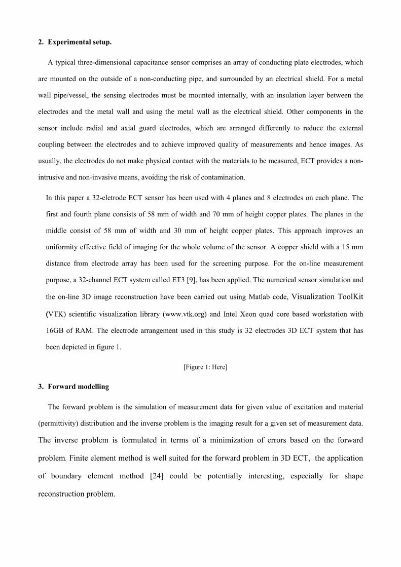
In this paper a 32-eletrode ECT sensor has been used with 4 planes and 8 electrodes on each plane. The

first and fourth plane consists of 58 mm of width and 70 mm of height copper plates. The planes in the

middle consist of 58 mm of width and 30 mm of height copper plates. This approach improves an

uniformity effective field of imaging for the whole volume of the sensor. A copper shield with a 15 mm

distance from electrode array has been used for the screening purpose. For the on-line measurement

purpose, a 32-channel ECT system called ET3 [9], has been applied. The numerical sensor simulation and

the on-line 3D image reconstruction have been carried out using Matlab code, Visualization ToolKit

(VTK) scientific visualization library (www.vtk.org) and Intel Xeon quad core based workstation with

16GB of RAM. The electrode arrangement used in this study is 32 electrodes 3D ECT system that has

been depicted in figure 1.

[Figure 1: Here]

3. Forward modelling

The forward problem is the simulation of measurement data for given value of excitation and material

(permittivity) distribution and the inverse problem is the imaging result for a given set of measurement data.

The inverse problem is formulated in terms of a minimization of errors based on the forward

problem. Finite element method is well suited for the forward problem in 3D ECT, the application

of boundary element method [24] could be potentially interesting, especially for shape

reconstruction problem.

We use low frequency approximation to the Maxwell’s equations. In a simplified mathematical model,

the electrostatic approximation 0=×∇ E is taken, effectively ignoring the effect of wave propagation. Let’s

take uE −∇= and assume no internal charges. Then the following equation holds.

0)( =∇⋅∇ uε in Ω (1)

where u is the electric potential, ε is dielectric permittivity and Ω is the region containing the field. The

potential on each electrode is known as

kVu = on electrode ek (2)

where ek is the k-th electrode held at the potential Vk. Using finite element method a linear system of

equation arises as

BUK =)(ε (3)

where the matrix K is the discrete representation of the operator ∇⋅∇ ε and the vector B is the boundary

condition term and U is the vector of electric potential solution. The total charge on the k-th electrode is

given by

2

ˆdx

a

uQ

kE n

k ∫ ∂∂

= ε (4)

where na is the inward normal on the k-th electrode, the surface integral of (3) is done over the surface of

electrode (ek) and the capacitance is calculated by C=Q/V. The Jacobian matrix S is calculated using an

efficient method [15]. Each raw of the Jacobian matrix is the sensitivity of one measurement as a result of

small change in each voxel in the imaging area. In other word, an element of the Jacobian matrix is the

derivative of the measured capacitance at the boundary divided to the derivative of permittivity of a voxel

[7]. An efficient formulation to calculate the Jacobian matrix uses the results of the forward problems and

mutual energy concept to calculate the Jacobian matrix [4, 15]. The solution of the forward problem and

the Jacobian matrix is used to solve the inverse problem, which is the estimation of the permittivity

distribution given the measured capacitance data.

4. 4D inversion

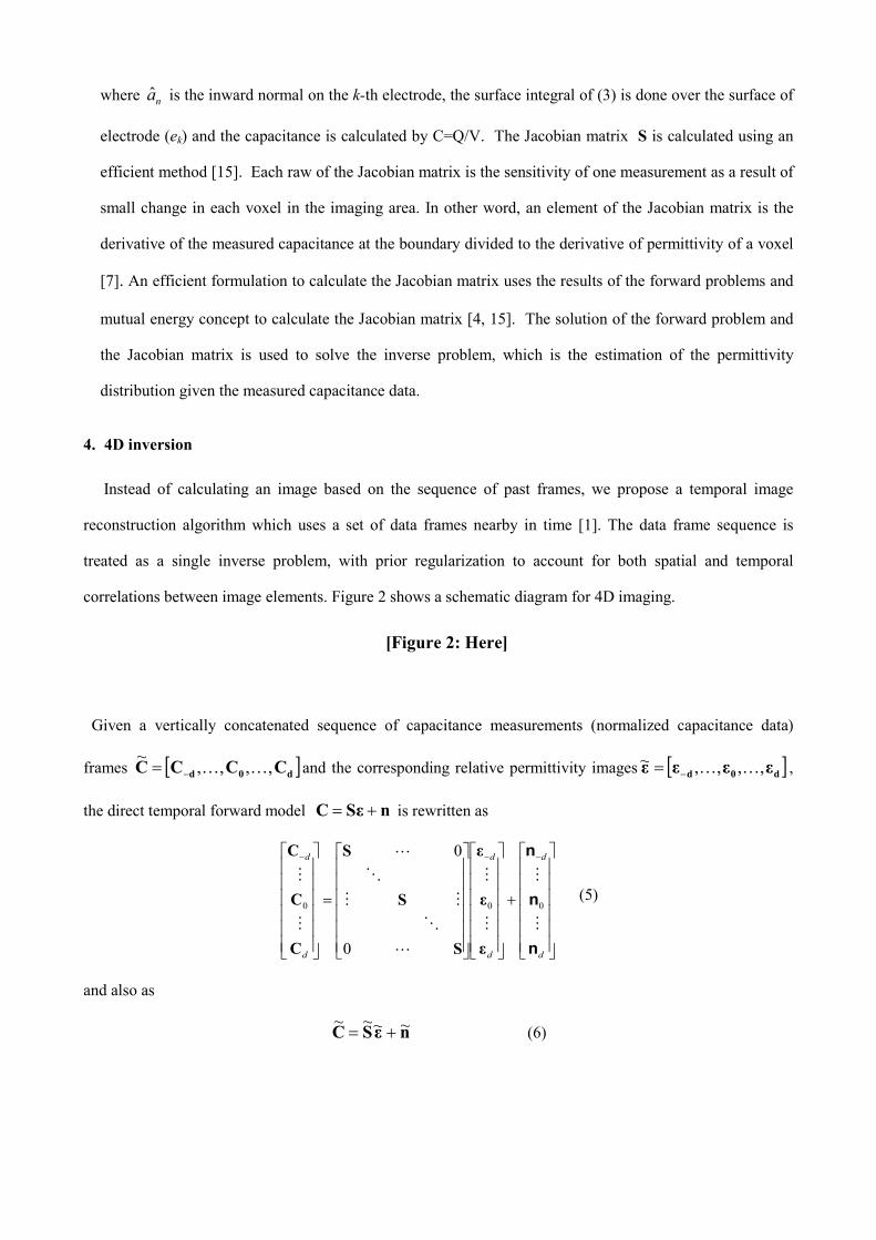
Instead of calculating an image based on the sequence of past frames, we propose a temporal image

reconstruction algorithm which uses a set of data frames nearby in time [1]. The data frame sequence is

treated as a single inverse problem, with prior regularization to account for both spatial and temporal

correlations between image elements. Figure 2 shows a schematic diagram for 4D imaging.

[Figure 2: Here]

Given a vertically concatenated sequence of capacitance measurements (normalized capacitance data)

frames [ ]d0d CCCC ,,,,~

KK−= and the corresponding relative permittivity images [ ]d0d εεεε ,,,,~KK−= ,

the direct temporal forward model nSεC += is rewritten as

+

=

−−−

d

d

d

d

d

d

n

n

n

M

M

M

M

L

O

MM

O

L

M

M

000

0

0

ε

ε

ε

S

S

S

C

C

C

(5)

and also as

nεSC ~~~~+= (6)

where [ ]dd nnnnnnnnnnnnnnnn ;;;;~

0 KK−= is the noise in the measured data. We assume S to be constant, although

this formulation could be modified to account for a time variation in S . Based on this

approximation SIS ⊗=~

, where the identity IIII has size 2d+1, and ⊗ is the Kronecker product.

The correlation of corresponding elements between adjacent frames (delay t=1) can be evaluated by an inter-

frame correlationγ , which has value between 0 (independent) and 1 (fully dependent). As the frames

become separated in time, the inter-frame correlation decreases; for an inter-frame separation t, the inter-

frame correlation is tγ . Frames with large time lag, |t|>d, can be considered independent. Image

reconstruction is then defined in terms of minimizing the augmented expression:

2

~~R

+

−

−−−

d

0

d

2

2

Wd

0

d

d

0

d

ε

ε

ε

ε

ε

ε

S0

S

0S

C

C

C

M

M

M

M

L

O

MM

O

L

M

M

λ (7)

and the inversion can be written as

11T-1T-1 )WSRS(SRB −−+=~~~~~~~ 2λ (8)

where WIW ⊗=~

and WWWW is regularization matrix for the measurement noise (in context of Tikhonov

regularization, ∑−=

12

nnW σ , where nσ is the average measurement noise), WWWW~ is diagonal since

measurement noise is uncorrelated between frames. This paper uses model, W = I. Here λ is the regularization

parameter. RΓR ⊗= -1~, R is the regularization matrix ( ∑−

=1

εεσR where εσ is a priori amplitude of

permittivity changes and R~ includes the temporal and spatial changes of permttivity) that represents the

spatial correlations between image voxels (The regularization matrix R may be understood to model the

"unlikelihood" of image element configurations) and Γ is the temporal weight matrix of an image sequence ε~

and is defined to have the form as

=

−

−−

−−

−

1

1

1

1

γγγγγγ

γγγγγγ

L

L

MMOMM

L

L

122

2212

1222

212

dd

dd

dd

dd

Γ (9)

From (8) and (9),

( )[ ] ( ) ( )[ ] 1~ −⊗+⊗⊗= VISPSΓ.PSΓB

2TT λ (10)

where P=R-1 and

V=W

-1. In practice, P and V are modeled directly from the system covariances, rather

than the inverse of R and W. 4D image can be reconstructed as

CB

ε

ε

ε

d

0

d

~~

~

~

~

=

−

M

M (11)

Although this estimate is an augmented image sequence, we are typically only interested in the current

image 0ε~ . It is calculated by CB

~~~0=0ε where 0BBBB

~ is the rows 1)(dn1dn MM +×+ K of BBBB~ , where nM is

number of measurements, in this paper for 32 electrodes ECT system nM =496. The size of the inverse

problem in proposed 4D algorithm is the number of measurements rather than number of voxels.

This will directly generate a 4D (movie) of the ECT image. If one wants to update the Jacobian and

dynamically select the regularization parameters, then the calculation of B~ needs be done in each

iteration of the 4D algorithm (each time that we have a new ECT data set). If we select a sigle set of

regularization parameter and accept linear inverse problem the calculation of B~ can be done

offline so the 4D algorithm becomes very fast.

If a priori knowledge of temporal change in permittivity is available (this could be developed by a

physical model, i.e. fluid dynamic model for flow visualization), then we can select an optimal

value for temporal correlation parameter. The γ is a parameter of the system; it depends on the

data acquisition frame rate, the speed of underlying permittivity changes and the noise level in

measurement system. A method to estimate the value of γ from measurement sequence will be

resented here. By taking covariance on both sides of (6), we have the estimated covariance matrix

of the data as

∑∑∑ += n

t

CSS ~~

^

~~~

ε (12)

the optimal γ is chosen so that the error between the true data covariance matrix ∑ C~ and the

estimated one ∑^

~Cis minimized as

2

~~~~~

minarg

F

t

nCSS∑∑∑ −−= ε

γγ (13)

where subscript F is a matrix norm (Euclidean norm). Since ∑∑ ⊗Γ= εε~ and SIS ⊗=~

,

(13) becomes

2

~~minarg

F

t

nCSS

⊗Γ−−= ∑∑∑ ε

γγ (14)

By taking covariance on both sides of nSεC += , we have

∑∑ ∑ += n

t

C SS ε (15)

so that ∑∑∑ −= nC

tSS ε ; we also have ∑∑ ⊗= nn I~ and ∑∑ ⊗Γ= CCC~ , where

)12()12( +×+∈Γ dd

C R is the correlation matrix of C~. Thus the optimal γ is calculated by

2

minarg

F

ncncc I

−⊗Γ−⊗−⊗Γ= ∑∑∑∑

γγ (16)

CΓ and ∑ C can be calculated directly from the data. ∑ n can be measured by calibration of ECT

system. For computational efficiency, (16) can be simplified as

2222

minarg

FF

nC

F

n

F

CC I ∑∑∑∑ −Γ−−Γ=γ

γ (17)

where CΓ ,

2

F

C∑ ,

2

F

n∑ and

2

F

nC ∑∑ − may be precalculated. Since Γ is relatively small

( )12()12( +×+ ddR ) this optimization can be performed directly by bisection search between limits.

Assuming linear image reconstruction of (15) enabled us to develop an estimation of temporal

parameter in (17) that only depends on covariance related to the measurement. An estimation

method that takes into account nonlinearly between data and image (dynamical image here) is

beyond scope of this paper.

5. Experimental results

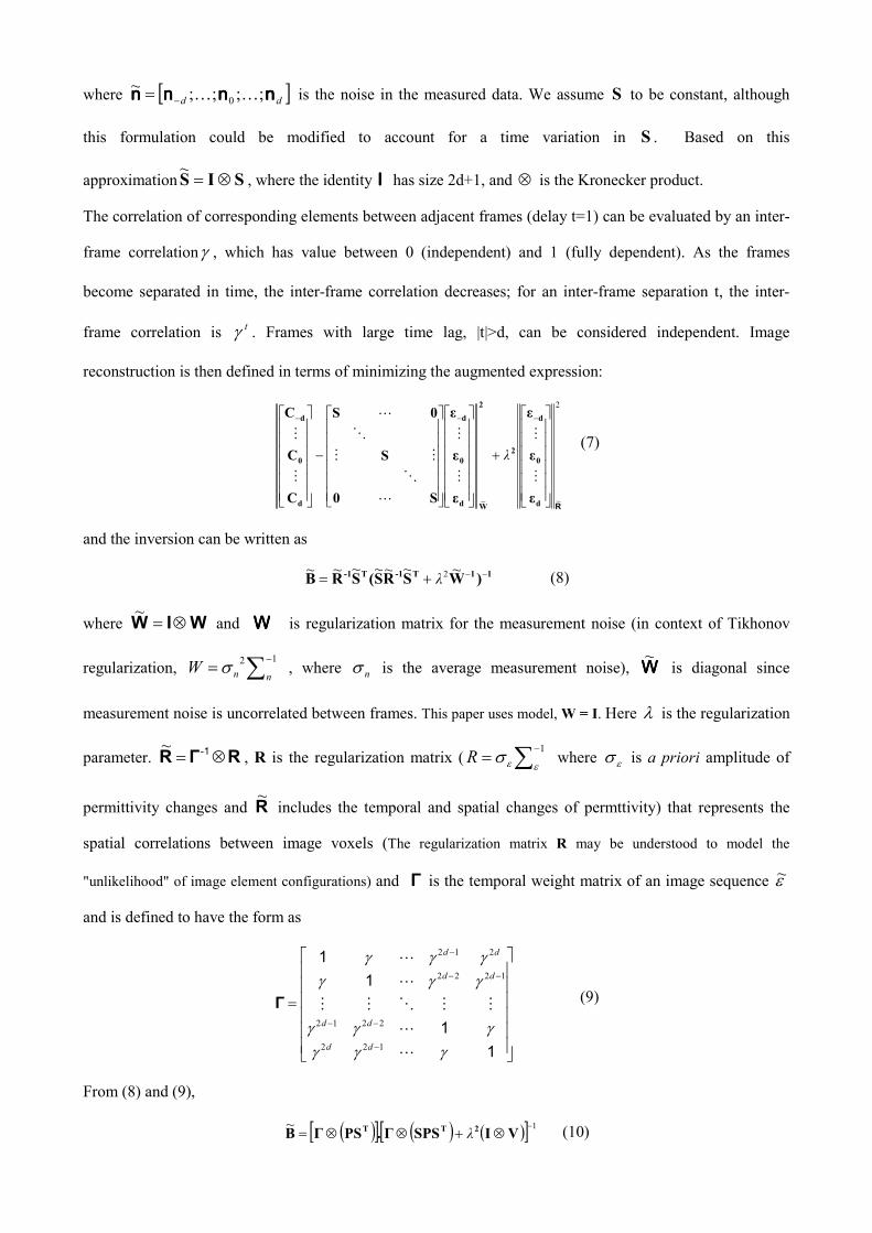
In order to evaluate the performance of proposed method compared to traditional single step Gauss-

Newton (but uncorrelated, here we call it 3D), synthetic data was generated using the same mesh.

Spherical inclusion with permittivity 1.6 and radius 2.5cm was centred in 7 different places starting

from the corner (1cm from the electrodes) to the centre of the imaging area with the 2cm steps. The

synthetic data was generated using a same mesh and up to 6% noise was added to the measure data.

The percentage of random Gaussian noise was selected with respect to the average value of all

measured capacitances. This figure shows superiority of the temporal image reconstruction with the

high noise data. We repeated the same test with 0% and 2%, 3% and 6% added noise and Figure 3

shows the norm of the error between reconstructions in all three noise levels. Assuming truε is true

permittivity and recε is reconstructed permittivity, the image error is defined as true

rectrue

εεε −

.

Temporal method works similar to the linear (temporally uncorrelated method) for noise free data

and outperforms the linear uncorrelated algorithm (3D) in higher noise levels, suggesting a better

noise performance. In all simulated and experimental results we select tw=0.8 (temporal

regularization parameter) and 2λ =10-4. These are seleced imperically in this study based on the fact

that they produce satisfactory results. In real life applications (say for multi-phase flow application)

these parameters have to be selected based on the physical reality of the experimental condition.

[Figure 3: Here]

The proposed algorithm has been tested against several experimental examples of moving 3D objects

(4D). Figure 4 shows the reconstructed images for different moving objects in a tank. The movie includes

several frames; here we only show few frames of the movie. The results presented in figure 4 are among

the first experimental results from proposed algorithm. In all cases 4D algorithms successfully

reconstructed the movement of 3D object. The algorithm was also applied to two more experimental

examples, similar results were observed in capturing dynamic of a moving 3D object (i.e. plastic rod) –

see figure 4. We have attached to this paper the movies related to each of these 4 experiments.

During the first two experiments we were using a cylindrical object with 150 mm of diameter and a

concentrically drilled hole with 50 mm of diameter and a rod of the same diameter, respectively. The

cylinder and the rod both had been made from Ertalon with relative permittivity of 3.2. Firstly the rod was

being put with a constant velocity of about 2cm/s near the wall of pipe. The rod was being pulled out

from the bigger cylinder as the next experiment. The velocity of rod movement has been well-matched to

the measurement abilities of used ET3 system which is now able to measure data in 32 channel mode

with up to 15 frames per second [9]. It can be observed that 4D algorithm allows for on-line visualization

of such objects in the whole volume of the sensor. In the next two experiments we moved two balls inside

a pipe. The first ball was 70 mm in diameter and the second one was 100 mm in diameter both filled with

plastic granulate (relative permittivity of 2.6). We let these balls move freely through the pipe with

constant velocity acquiring measurement data simultaneously. The results we have got using 4D

algorithm are promising even though the velocity of balls was too high. It can be easily observed that

some axial resolution limitations of a 3D capacitance sensor in the lower and upper part of the imaging

volume exist which is obvious because of sensor coverage. The central area of the sensor volume

characterizes relatively low sensitivity. Nevertheless the ball movement in that area has been visualized

with acceptable quality regardless of poor sensitivity. The main bottleneck in these experiments we had to

face with was the ET3 capacitance system which is now relatively slow in 32 channel mode. With faster

and less noisy ECT system the quality of 4D images for on-line visualization would be improved. In

order to implement a temporal solver in an ECT system for real-time imaging, a delay must be

introduced between the measurements and reconstruction to allow acquisition of d ``future

frames''. This corresponds to the linear phase filters used in digital signal processing

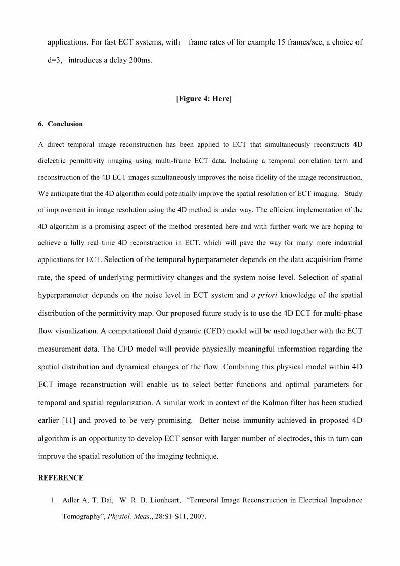
applications. For fast ECT systems, with frame rates of for example 15 frames/sec, a choice of

d=3, introduces a delay 200ms.

[Figure 4: Here]

6. Conclusion

A direct temporal image reconstruction has been applied to ECT that simultaneously reconstructs 4D

dielectric permittivity imaging using multi-frame ECT data. Including a temporal correlation term and

reconstruction of the 4D ECT images simultaneously improves the noise fidelity of the image reconstruction.

We anticipate that the 4D algorithm could potentially improve the spatial resolution of ECT imaging. Study

of improvement in image resolution using the 4D method is under way. The efficient implementation of the

4D algorithm is a promising aspect of the method presented here and with further work we are hoping to

achieve a fully real time 4D reconstruction in ECT, which will pave the way for many more industrial

applications for ECT. Selection of the temporal hyperparameter depends on the data acquisition frame

rate, the speed of underlying permittivity changes and the system noise level. Selection of spatial

hyperparameter depends on the noise level in ECT system and a priori knowledge of the spatial

distribution of the permittivity map. Our proposed future study is to use the 4D ECT for multi-phase

flow visualization. A computational fluid dynamic (CFD) model will be used together with the ECT

measurement data. The CFD model will provide physically meaningful information regarding the

spatial distribution and dynamical changes of the flow. Combining this physical model within 4D

ECT image reconstruction will enable us to select better functions and optimal parameters for

temporal and spatial regularization. A similar work in context of the Kalman filter has been studied

earlier [11] and proved to be very promising. Better noise immunity achieved in proposed 4D

algorithm is an opportunity to develop ECT sensor with larger number of electrodes, this in turn can

improve the spatial resolution of the imaging technique.

REFERENCE

1. Adler A, T. Dai, W. R. B. Lionheart, “Temporal Image Reconstruction in Electrical Impedance

Tomography”, Physiol. Meas., 28:S1-S11, 2007.

2. Chen, G. P, W. B. Yu, Z. Q. Zhao, Z. P. Nie, Q. H. Liu, “The prototype of microwave-

induced thermo-acoustic tomography imaging by time reversal mirror”, Journal of

electromagnetic waves and applications, Vol.: 22 , Issue: 11-12 , Pages: 1565-1574,

2008.

3. Cheng, X. X. , B. I. Wu, H. Chen, J.A. Kong, “ Imaging of objects through lossy layer with

defects”, Progress in electromagnetics research-pier, Vol.: 84, Pages: 11-26, 2008.

4. Li Y. and W. Q. Yang, “Image reconstruction by nonlinear Landweber iteration for

complicated distributions”, Meas. Sci. Technol. 19, 094014 (8pp), 2008.

5. Huang C. H., Y. F. Chen, C. C. Chiu, “Permittivity distribution reconstruction of dielectric

objects by a cascaded method”, Journal of electromagnetic waves and applications, Vol.:

21, Issue: 2, Pages: 145-159, 2007.

6. Franceschini, G. , M. Donelli, D. Franceschini, M. Benedetti, P. Rocca, A. Massa,

“Microwave imaging from amplitude-only data-advantages and open problems of a two-step

multi-resolution strategy”, Progress in electromagnetics research-pier , Vol.: 83, Pages:

397-412 , 2008.

7. Marashdeh Q. , W. Warsito, L. S. Fan, L. T. Teixeira, “A nonlinear image reconstruction

technique for ECT using a combined neural network approach,” Meas. Sci. Technol. 17 No

8 , 2097-2103, 2006.

8. Nurge M. A., “Electrical capacitance volume tomography with high contrast dielectrics

using a cuboid sensor geometry”, Meas. Sci. Technol. 18 No 5 , 1511-1520, 2007.

9. Olszewski T., P. Brzeski, J. Mirkowski, A. Pląskowski, W. Smolik, R. Szabatin, “Modular

Capacitance Tomograph”, Proc 4th International Symposium on Process Tomography in Warsaw,

2006.

10. Romanowski A., K. Grudzien, R. Banasiak, R. A. Williams, D. Sankowski, “Hopper Flow

Measurement Data Visualization: Developments Towards 3D”, Proc 5th World Congress on

Industrial Process Tomography, Bergen, Norway, 2006.

11. Seppanen A., M. Vauhkonen, P. Vauhkonen, E. Somersalo, J. P. Kaipio , “Fluid dynamical

models and state estimation in process tomography: Effect due to inaccuracies in flow

fields”, Journal of electronic imaging, 10, 3, 630-640, 2001 .

12. Schmitt U. , A. K. Louis, “ Efficient Algorithms for the Regularization of dynamic inverse

Problems - Part I : Theory”, Inverse Problems, 18, 645-658, 2002.

13. Schmitt, U., A. K. Louis, C. H. Wolters, M. Vauhkonen, “Efficient algorithms for the

regularization of dynamic inverse problems: II. Applications.”, Inverse Problems, 18 (3),

pp.659-676, 2002.

14. Serdyuk V. M., “Dielectric study of bound water in grain at radio and microwave

frequencies”, Progress in electromagnetics research-pier, Vol.: 84, Pages: 379-406, 2008.

15. Soleimani M., “Three-dimensional electrical capacitance tomography imaging”, Insight, Non-

Destructive Testing and Condition Monitoring, Vol. 48, No. 10, Pages: 613-617, 2006.

16. Soleimani M., M. Vauhkonen, W. Q. Yang, A. J. Peyton, B. S. Kim, X. Ma, “Dynamic

imaging in electrical capacitance tomography and electromagnetic induction tomography

using a Kalman filter”, Meas. Science. Tech. 18 (11), pages: 3287-3294, 2007.

17. Soleimani M., H. Wang, Y. Li, W. Q. Yang, “A comparative study of three dimensional electrical

capacitance tomography”, International Journal for Information Systems Sciences, Vol.3, No.2: 283-

291, 2007.

18. Wajman R., R. Banasiak, L. Mazurkiewicz, D. Dyakowski, D. Sankowski, “Spatial imaging with

3D capacitance measurements”, Meas. Sci. Technol. 17 No 8, Pages: 2113-2118, 2006.

19. Warsito W. , Q. Marashdeh, L. S. Fan, “Electrical capacitance volume tomography”, IEEE sensors

journal, Vol.: 7 Issue: 3-4 Pages: 525-535., 2007

20. Warsito W., L. S. Fan, “Development of 3-Dimensional Electrical Capacitance Tomography Based

on Neural Network Multi-criterion Optimization Image Reconstruction”, Proc. 3rd World Congress

on Industrial Process Tomography (Banff), Pages: 942-947, 2003.

21. Warsito W., L. S. Fan, “Imaging the Bubble Behavior Using the 3-D Electric Capacitance

Tomograph” Chem. Eng. Sci., 60 (22), 6073-6084, 2005.

22. Yang W.Q., “Key issues in designing capacitance tomography sensors”, IEEE Conference on

Sensors, Daegu, Korea, Pages: 497-505, 2006.

23. Yang W.Q., L. and Peng, “Review of image reconstruction algorithms for electrical capacitance

tomography, Part 1: Principles”, Proc International Symposium on Process Tomography in Poland

(Wroclaw), Pages: 123-132, 2002.

24. Zacharopoulos A., S. Arridge, “3D shape reconstruction in Optical Tomography using

spherical harmonics and BEM”, Journal of electromagnetic waves and applications, Vol.:

20, Issue: 13, Pages: 1827-1836, 2006.

25. Zhong X. M., C. Liao, W. Chen, Z. B. Yang, Y. Liao, F. B. Meng, “Image reconstruction

of arbitrary cross section conducting cylinder using UWB pulse”, Journal of

electromagnetic waves and applications, Vol.: 21 Issue: 1, Pages: 25-34, 2007.

Figures

(a)

(b)

Figure 1: 32 electrodes array for 3D ECT system a) 4 planes with 8 electrodes in each plane, b)

PCB layout with dimensions used for sensor fabrication

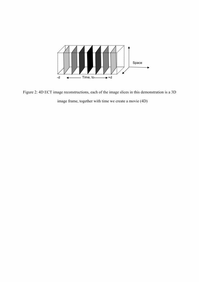
Figure 2: 4D ECT image reconstructions, each of the image slices in this demonstration is a 3D

image frame, together with time we create a movie (4D)

Space

Time, to -d +d

1 2 3 4 5 6 70.1076

0.1078

0.108

0.1082

0.1084

0.1086

0.1088

0.109

Position of sphere

Image error

1 2 3 4 5 6 70.1075

0.108

0.1085

0.109

0.1095

0.11

0.1105

Position of sphereImage error

(a) (b)

1 2 3 4 5 6 70.107

0.108

0.109

0.11

0.111

0.112

0.113

Position of sphere

Image error

1 2 3 4 5 6 70.108

0.11

0.112

0.114

0.116

0.118

0.12

0.122

0.124

Position of sphere

Image error

(c ) (d)

Figure 3: The error between simulated and real images using 3D (square) and 4D (triangle)

methods (a): Noise free (b) : 2 percent noise (c): 3 percent noise (d): 6 percent noise

Rod put in

(Movie1.avi)

Rod pulled out

(Movie2.avi)

Small ball

(Movie3.avi)

Large ball

(Movie4.avi)

Figure4: 4D ECT visualisation of moving objects: for each case the image is a snap shot of 4D

movie reconstruction for frames 45, 55, 135,185 out of 200 frames in each case