foundations of semantics ii: composition
TRANSCRIPT
Foundations of Semantics II: Composition
Rick Nouwen | [email protected]
February/March 2011, Gent
1 Compositionality
So far, we have only discussed what semantic meanings, truth-conditions, are, and what we are goingto use to write them down. The goal of a formal semantic theory is to provide a mechanism thatsystematically assigns truth-conditions (or representations thereof) to natural language sentences. Incontemporary semantics, we do this by means of a guiding principle (often attributed to Gottlob Frege):
The Compositionality Principle — The meaning of the whole is determined (solely) by themeaning of the parts and their mode of composition.
The intuition behind this principle is that meanings are derived by means of a fully productive mecha-nism. That is, we do not learn the meanings of sentences, we derive them from what we know about themeanings of words. So, we understand what the example in (1) means because we are acquainted withthe words in that sentence, even though this is the first time we have ever seen this particular sentence.
(1) The old cat sat in the middle of a huge square opposite a small church with a blue tower.
Discussion: one version of the compositionality principle states that the meaning of the whole isexhaustively determined by the meaning of the parts and their mode of composition. (The version with‘solely’ in the presentation above). Can you think of examples where this particular principle appearsto be too strong?
(If you have heard of indexicals before, think of examples with one or more indexicals in them.)
In semantics, we use compositionality as a general methodological principle. That is, we want oursemantics to be compositional, or at least as compositional as possible. This means that given a surfacestructure and a lexicon, the semantics allows us to determine the truth-conditions of the structure. So,the semantics does not tell us what the truth-conditions of John hates Mary are in any direct way, butit will tell us how to derive these truth-conditions given the structure ‘[ John [ hates Mary ] ]’ and themeaning of John, hate and Mary.
In terms of a referential theory of meaning, this means that the lexicon is responsible for stating thereference of individual words, while the compositional system is responsible for deriving the referenceof complex expressions.
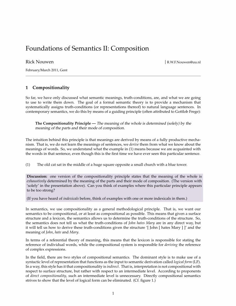
In the field, there are two styles of compositional semantics. The dominant style is to make use of asyntactic level of representation that functions as the input to semantic derivation called logical form (LF).In a way, this style has it that compositionality is indirect. That is, interpretation is not compositional withrespect to surface structure, but rather with respect to an intermediate level. According to proponentsof direct compositionality, such an intermediate level is unnecessary. Directly compositional semanticsstrives to show that the level of logical form can be eliminated. (Cf. figure 1.)
1
LogicalForm (LF)
Lexicon
Truth-conditions
Indirect Compositionality
SurfaceStructure
SurfaceStructure
Lexicon
Truth-conditions
Direct Compositionality
Figure 1: Direct versus indirect compositionality
In what follows, we shall focus on the indirectly compositional approach to natural language semantics.The main reason for this is that it is often insightful to use a level of logical form, especially since it allowsfor easy scrutiny of the relation between semantic and syntactic mechanisms. Let me illustrate with alook ahead. Consider the following example:
(2) Some woman loves every man.
This example is ambiguous. Here are two predicate logical formulae corresponding to the two readings:
(3) a. ∃x[woman(x) ∧ ∀y[man(y)→ love(x, y)]](there is some woman such that she loves every man; that is, she is indiscriminate in love)
b. ∀y[man(y)→ ∃x[woman(x) ∧ love(x, y)]](for every man in the world, we can find at least one woman who loves this man)
It is the reading in (3-b) that is a challenge to account for. As we will see in detail later, the reasonis because this reading seems to involve an ordering of the quantifiers in this sentence that does notcorrespond to the surface ordering. In (3-b), the existential quantifier is in the scope of the universalquantifier.
2
It is common in indirect compositionality approaches to account for (3-b) by making use of a form ofmovement. So, the two paraphrases in (3) correspond to two different logical forms, one in which nomovement took place and one in which the object quantifier moves to a higher position.
(4) a. [ some woman [ loves [ every man ]]]b. [ every man [ some woman [ loves ] ] ]
On the basis of these two logical forms, we can now compositionally derive two (distinct) truth-conditions, namely (3-a) for (4-a) and (3-b) for (4-b). (We’ll see how this works in detail later in thecourse). Crucial, however, is that prior to this compositional derivation, we needed to perform asyntactico-semantic operation on the purely representational level of LF.
In contrast, a directly compositional approach would account for the same ambiguity without havingto resort to movement, or any other method that necessitates a level like logical form. The easiest wayto do this (but there are important and more intricate techniques I cannot go into now) is by saying thattransitive verbs like love are ambiguous with respect to which argument has scope over which argument.
2 Functions and Types
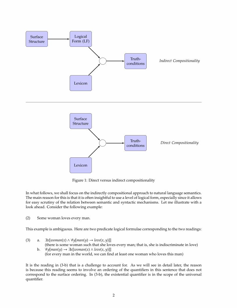
Puzzle— There is a logic behind the labeling of the nodes in this tree. Can you figure it out?
(5) t
〈t, t〉 t
〈〈e, t〉, t〉
〈〈e, t〉, 〈〈e, t〉, t〉〉 〈e, t〉
〈e, t〉
〈e, 〈e, t〉〉 e
〈〈e, t〉, e〉 〈e, t〉
The mechanism illustrated in the tree in (5) is that of function application, the main mode of compositionfor meaning derivation. Before we can explain the details of this mechanism and what (5) is meant torepresent, we have to make sure we understand what a function is.
2.1. Functions and Types
An example of a function is f in (6), which you may remember from a distant or not so distant schoolpast:
(6) f (x) = x + 1
3
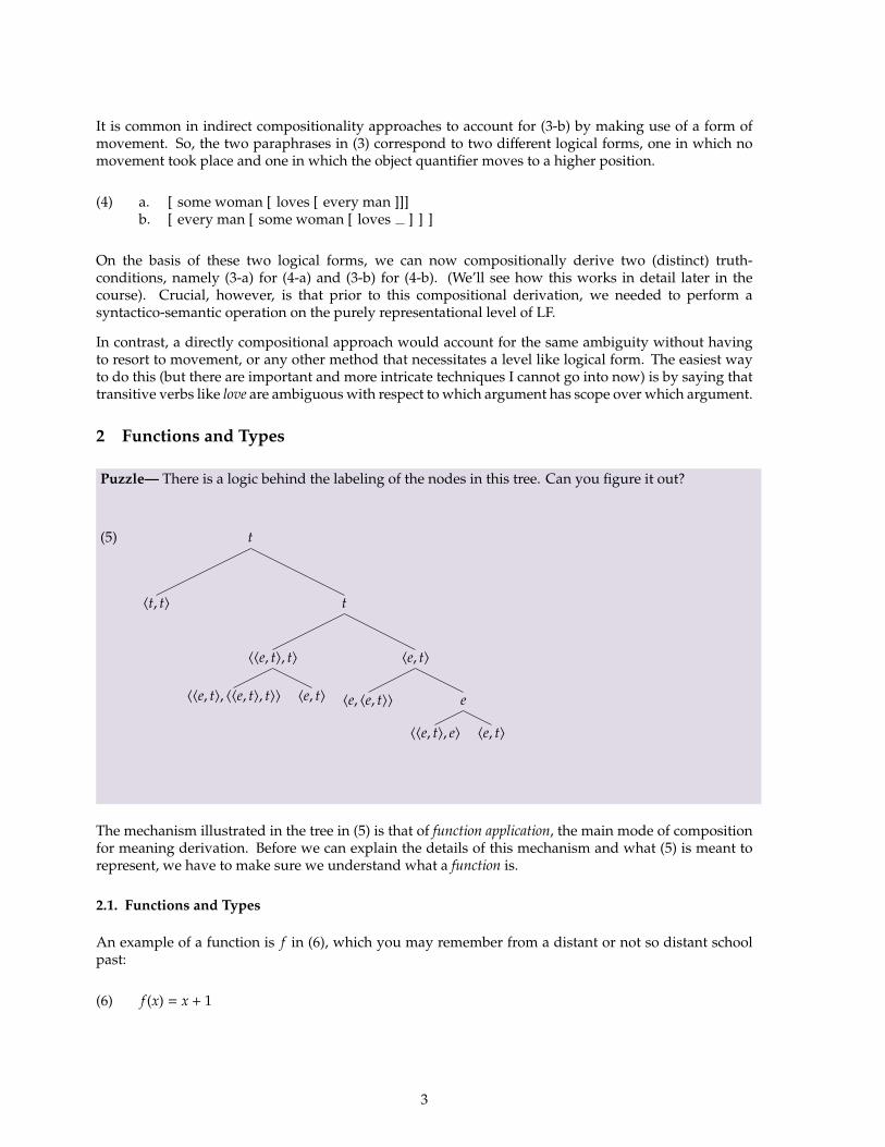
The function f adds 1 to any argument you feed the function. So, f (3) returns 3 + 1 (i.e. 4), f (352) returns353, etc. This is an instance of function application: you combine the function with an argument and getin return an output value. This value is derived from the argument in a systematic way, in this case byadding 1 to the argument. One way to represent the relation between function, argument and functionvalue is by means of a tree structure:
(7) 353
f 352
function value
function argument
Here’s another example from arithmetic:
(8) 4√ 16
As in predicate logic, it makes sense to distinguish variables from constants in the definition of functions.In the definition of f above, there is mention of ‘x’ and of ‘1’. Clearly, x is a variable. It is a place holderfor whatever argument we are going to combine the function with; it does not have a fixed reference. Incontrast, 1 is a constant: it refers to an entity with a unique set of properties.
The function f above targets arithmetic entities such as integers or reals. Since the operation + onlymakes sense with respect to numbers, it would be inappropriate to apply f to an individual like John.So, we know that the arguments f takes are of a particular type, namely that of numbers. Also, we knowthat any function value that results from applying f to an argument is also of that type. But now considerfunction g:
(9) g(x) = x’s age
Numbers don’t have an age: arguments of g must be living things. The function value resulting fromg being applied to something alive is a number, and so we conclude that g takes arguments of typeliving things to return function values of type numbers. On the basis of this, we can specify the type of thefunction. We do this by combining the type of the arguments and the type of the function values in anordered pair. For instance, the type of g is 〈living things,numbers〉. The type of f is 〈numbers,numbers〉.
We indicate types with colons, as follows:
(10) a. f : 〈numbers,numbers〉b. 324 : numbersc. John : living thingsd. g : 〈living things,numbers〉
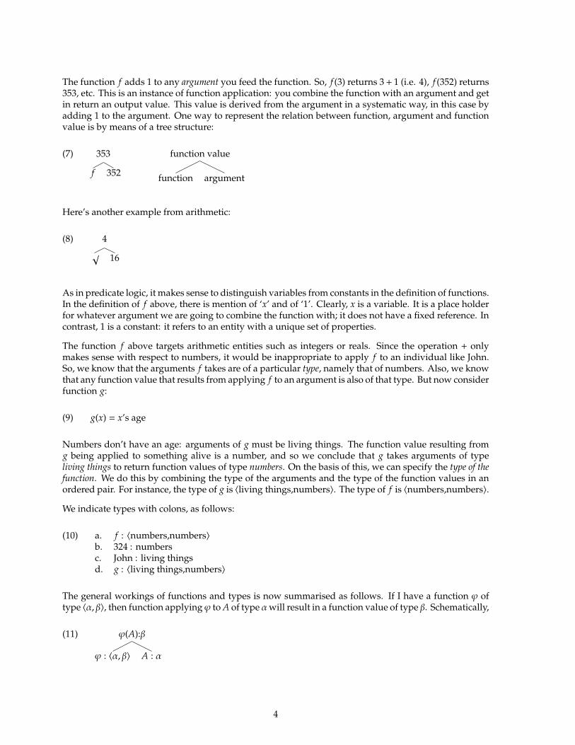
The general workings of functions and types is now summarised as follows. If I have a function ϕ oftype 〈α, β〉, then function applyingϕ to A of type αwill result in a function value of type β. Schematically,
(11) ϕ(A):β
ϕ : 〈α, β〉 A : α
4
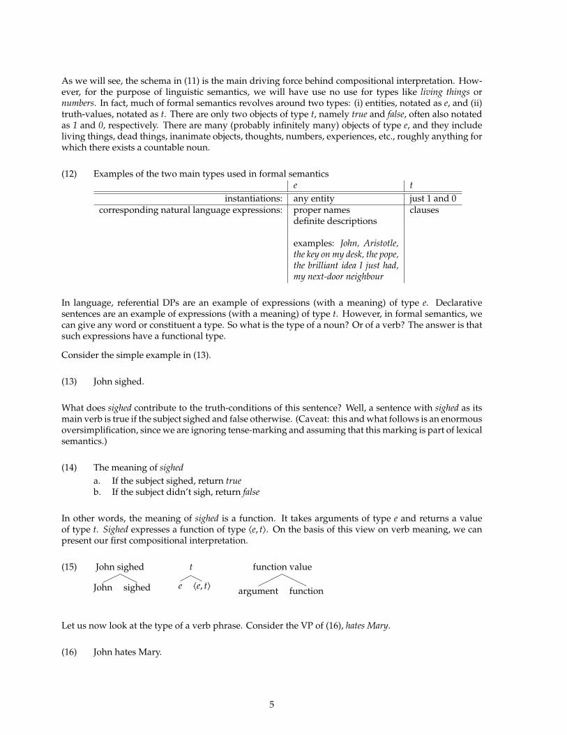
As we will see, the schema in (11) is the main driving force behind compositional interpretation. How-ever, for the purpose of linguistic semantics, we will have use no use for types like living things ornumbers. In fact, much of formal semantics revolves around two types: (i) entities, notated as e, and (ii)truth-values, notated as t. There are only two objects of type t, namely true and false, often also notatedas 1 and 0, respectively. There are many (probably infinitely many) objects of type e, and they includeliving things, dead things, inanimate objects, thoughts, numbers, experiences, etc., roughly anything forwhich there exists a countable noun.
(12) Examples of the two main types used in formal semanticse t
instantiations: any entity just 1 and 0corresponding natural language expressions: proper names clauses
definite descriptions
examples: John, Aristotle,the key on my desk, the pope,the brilliant idea I just had,my next-door neighbour
In language, referential DPs are an example of expressions (with a meaning) of type e. Declarativesentences are an example of expressions (with a meaning) of type t. However, in formal semantics, wecan give any word or constituent a type. So what is the type of a noun? Or of a verb? The answer is thatsuch expressions have a functional type.
Consider the simple example in (13).
(13) John sighed.
What does sighed contribute to the truth-conditions of this sentence? Well, a sentence with sighed as itsmain verb is true if the subject sighed and false otherwise. (Caveat: this and what follows is an enormousoversimplification, since we are ignoring tense-marking and assuming that this marking is part of lexicalsemantics.)
(14) The meaning of sigheda. If the subject sighed, return trueb. If the subject didn’t sigh, return false
In other words, the meaning of sighed is a function. It takes arguments of type e and returns a valueof type t. Sighed expresses a function of type 〈e, t〉. On the basis of this view on verb meaning, we canpresent our first compositional interpretation.
(15) John sighed
John sighed
t
e 〈e, t〉
function value
argument function
Let us now look at the type of a verb phrase. Consider the VP of (16), hates Mary.
(16) John hates Mary.
5
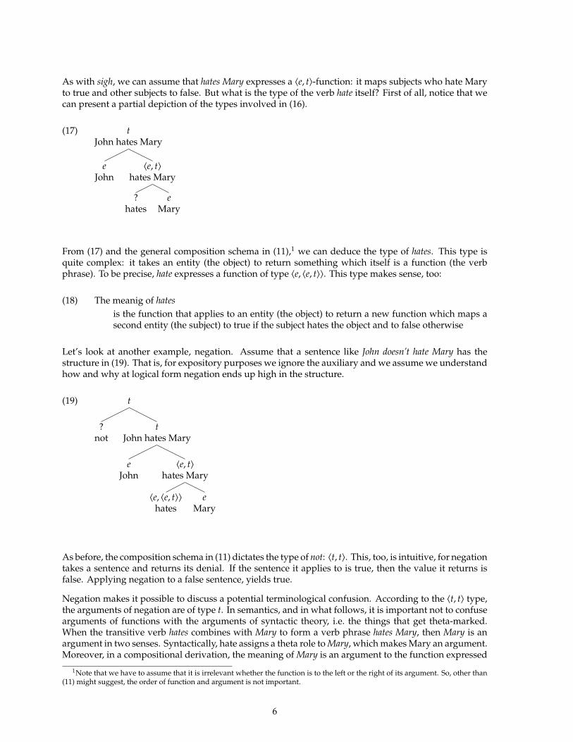
As with sigh, we can assume that hates Mary expresses a 〈e, t〉-function: it maps subjects who hate Maryto true and other subjects to false. But what is the type of the verb hate itself? First of all, notice that wecan present a partial depiction of the types involved in (16).
(17) tJohn hates Mary
eJohn
〈e, t〉hates Mary
?hates
eMary
From (17) and the general composition schema in (11),1 we can deduce the type of hates. This type isquite complex: it takes an entity (the object) to return something which itself is a function (the verbphrase). To be precise, hate expresses a function of type 〈e, 〈e, t〉〉. This type makes sense, too:
(18) The meanig of hatesis the function that applies to an entity (the object) to return a new function which maps asecond entity (the subject) to true if the subject hates the object and to false otherwise
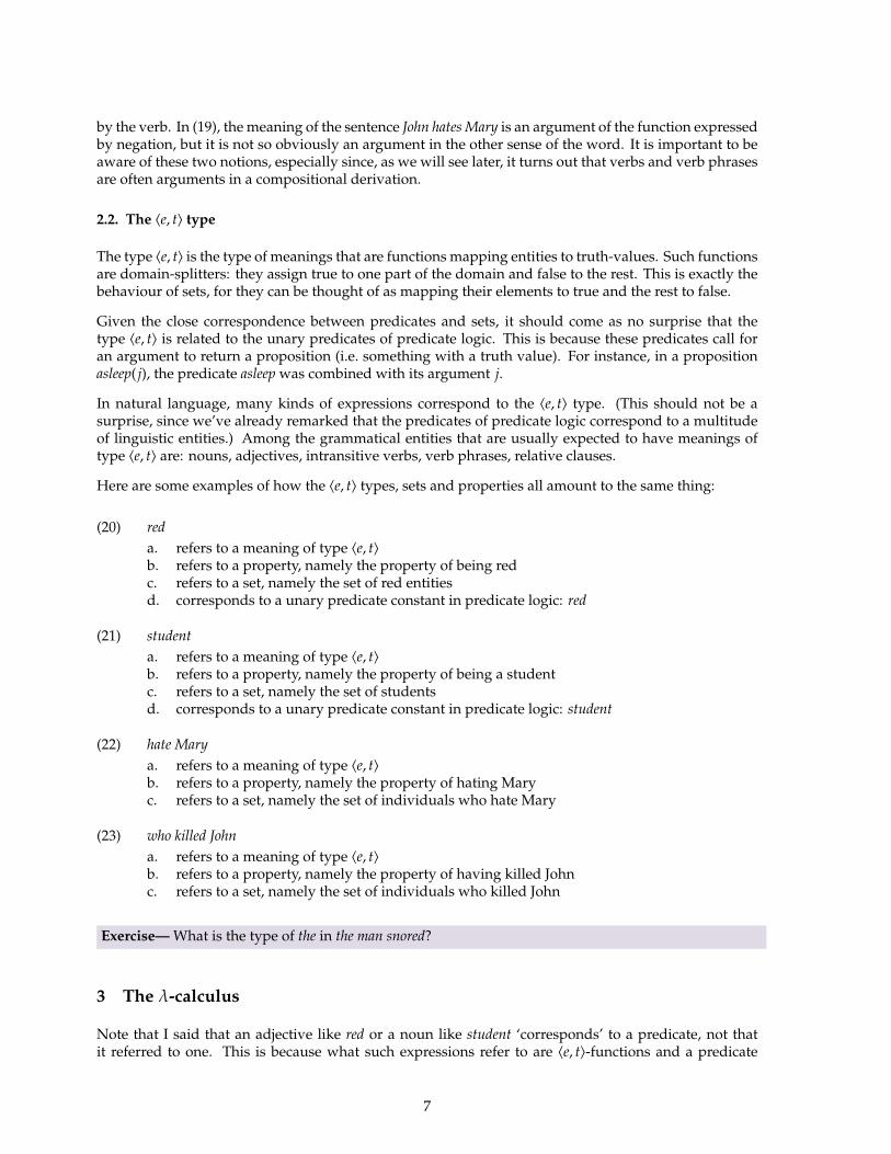
Let’s look at another example, negation. Assume that a sentence like John doesn’t hate Mary has thestructure in (19). That is, for expository purposes we ignore the auxiliary and we assume we understandhow and why at logical form negation ends up high in the structure.
(19) t
?not
tJohn hates Mary
eJohn
〈e, t〉hates Mary
〈e, 〈e, t〉〉hates
eMary
As before, the composition schema in (11) dictates the type of not: 〈t, t〉. This, too, is intuitive, for negationtakes a sentence and returns its denial. If the sentence it applies to is true, then the value it returns isfalse. Applying negation to a false sentence, yields true.
Negation makes it possible to discuss a potential terminological confusion. According to the 〈t, t〉 type,the arguments of negation are of type t. In semantics, and in what follows, it is important not to confusearguments of functions with the arguments of syntactic theory, i.e. the things that get theta-marked.When the transitive verb hates combines with Mary to form a verb phrase hates Mary, then Mary is anargument in two senses. Syntactically, hate assigns a theta role to Mary, which makes Mary an argument.Moreover, in a compositional derivation, the meaning of Mary is an argument to the function expressed
1Note that we have to assume that it is irrelevant whether the function is to the left or the right of its argument. So, other than(11) might suggest, the order of function and argument is not important.
6
by the verb. In (19), the meaning of the sentence John hates Mary is an argument of the function expressedby negation, but it is not so obviously an argument in the other sense of the word. It is important to beaware of these two notions, especially since, as we will see later, it turns out that verbs and verb phrasesare often arguments in a compositional derivation.
2.2. The 〈e, t〉 type
The type 〈e, t〉 is the type of meanings that are functions mapping entities to truth-values. Such functionsare domain-splitters: they assign true to one part of the domain and false to the rest. This is exactly thebehaviour of sets, for they can be thought of as mapping their elements to true and the rest to false.
Given the close correspondence between predicates and sets, it should come as no surprise that thetype 〈e, t〉 is related to the unary predicates of predicate logic. This is because these predicates call foran argument to return a proposition (i.e. something with a truth value). For instance, in a propositionasleep( j), the predicate asleep was combined with its argument j.
In natural language, many kinds of expressions correspond to the 〈e, t〉 type. (This should not be asurprise, since we’ve already remarked that the predicates of predicate logic correspond to a multitudeof linguistic entities.) Among the grammatical entities that are usually expected to have meanings oftype 〈e, t〉 are: nouns, adjectives, intransitive verbs, verb phrases, relative clauses.
Here are some examples of how the 〈e, t〉 types, sets and properties all amount to the same thing:
(20) reda. refers to a meaning of type 〈e, t〉b. refers to a property, namely the property of being redc. refers to a set, namely the set of red entitiesd. corresponds to a unary predicate constant in predicate logic: red
(21) studenta. refers to a meaning of type 〈e, t〉b. refers to a property, namely the property of being a studentc. refers to a set, namely the set of studentsd. corresponds to a unary predicate constant in predicate logic: student
(22) hate Marya. refers to a meaning of type 〈e, t〉b. refers to a property, namely the property of hating Maryc. refers to a set, namely the set of individuals who hate Mary
(23) who killed Johna. refers to a meaning of type 〈e, t〉b. refers to a property, namely the property of having killed Johnc. refers to a set, namely the set of individuals who killed John
Exercise— What is the type of the in the man snored?
3 The λ-calculus
Note that I said that an adjective like red or a noun like student ‘corresponds’ to a predicate, not thatit referred to one. This is because what such expressions refer to are 〈e, t〉-functions and a predicate
7
constant is not such a function, but is rather a name for something that in predicate logic is interpretedas such. There is a way to extend predicate logic, however, to express directly the relation between typesand meanings. This is done by means of the so-called lambda calculus.
To get the intuition, let us first consider a simple unary predicate like red. In predicate logic, red is notby itself a very meaningful expression. It does not specify, for instance, how many arguments it needsin order to form a proposition. With the lambda calculus we can express precisely what is needed tosaturate the arguments of predicates. More generally, with the lambda calculus one has a language thatcan express functions and their application, in a very precise way.
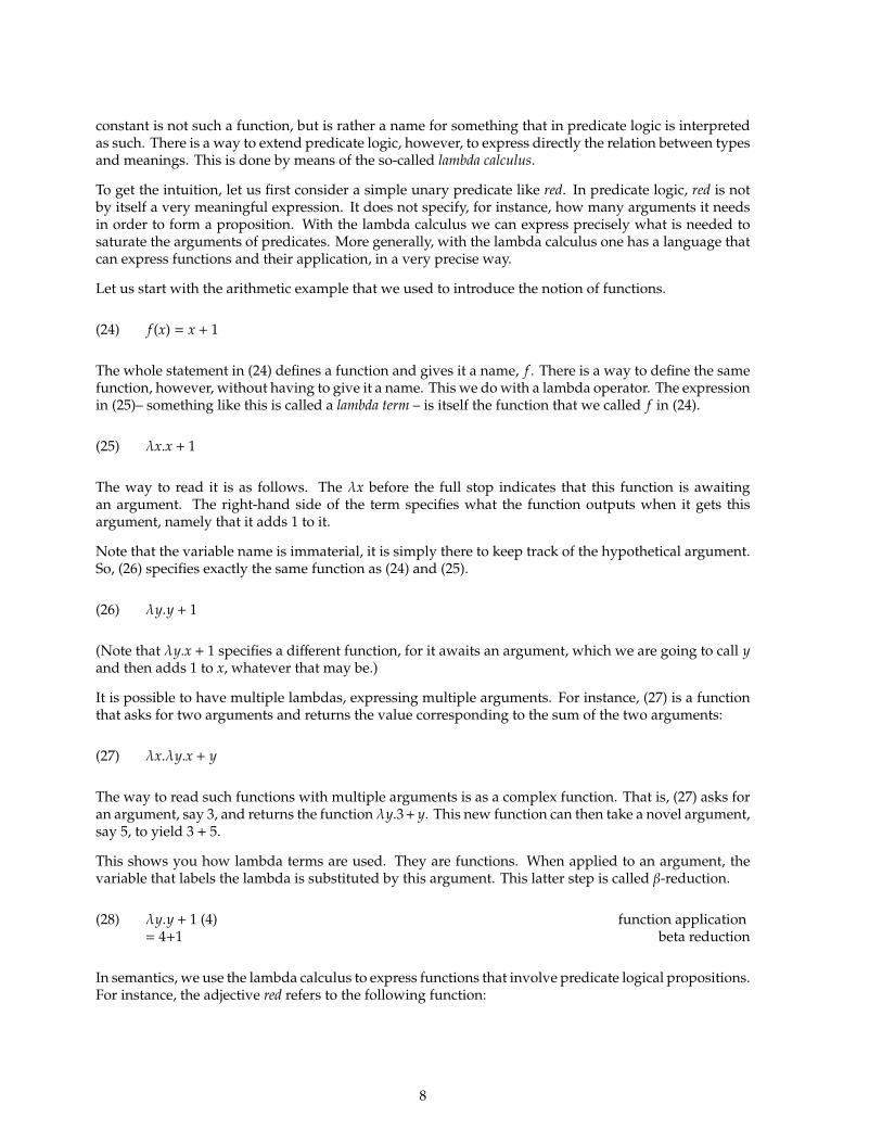
Let us start with the arithmetic example that we used to introduce the notion of functions.
(24) f (x) = x + 1
The whole statement in (24) defines a function and gives it a name, f . There is a way to define the samefunction, however, without having to give it a name. This we do with a lambda operator. The expressionin (25)– something like this is called a lambda term – is itself the function that we called f in (24).
(25) λx.x + 1
The way to read it is as follows. The λx before the full stop indicates that this function is awaitingan argument. The right-hand side of the term specifies what the function outputs when it gets thisargument, namely that it adds 1 to it.
Note that the variable name is immaterial, it is simply there to keep track of the hypothetical argument.So, (26) specifies exactly the same function as (24) and (25).
(26) λy.y + 1
(Note that λy.x + 1 specifies a different function, for it awaits an argument, which we are going to call yand then adds 1 to x, whatever that may be.)
It is possible to have multiple lambdas, expressing multiple arguments. For instance, (27) is a functionthat asks for two arguments and returns the value corresponding to the sum of the two arguments:
(27) λx.λy.x + y
The way to read such functions with multiple arguments is as a complex function. That is, (27) asks foran argument, say 3, and returns the function λy.3+ y. This new function can then take a novel argument,say 5, to yield 3 + 5.
This shows you how lambda terms are used. They are functions. When applied to an argument, thevariable that labels the lambda is substituted by this argument. This latter step is called β-reduction.
(28) λy.y + 1 (4) function application= 4+1 beta reduction
In semantics, we use the lambda calculus to express functions that involve predicate logical propositions.For instance, the adjective red refers to the following function:
8
(29) λx.red(x)
This function awaits an argument (x) and returns a predicate logical proposition that consists of thepredicate red with the function’s argument as its argument. So, if we apply the function in (29) to j,through beta reduction we will end up with the proposition red( j). If we apply the function in (29) to y,we end up with red(y), etc.
The benefit of the lambda calculus is that we now have a way to express complex properties / sets. Say,for instance, that our predicate logic has among its unary predicate constants the predicates lazy andpro f essor, then (30) expresses the property of being a lazy professor (i.e. the set of lazy professors):
(30) λx.lazy(x) ∧ pro f essor(x)
If we apply (30) to an argument it will return a proposition that is only true if the argument is both lazy anda professor. So apply it to John, j, a lazy student, and the output proposition will be lazy( j)∧ pro f essor( j),which will be false; apply it to Mary, m, a lazy professor, and the output is lazy(m) ∧ pro f essor(m), whichwill be true.
Here is an example of a complex verb phrase meaning:
(31) λy.hate(y, j) ∧ ¬hate(y,m)
This function takes an argument (y) and returns a proposition that says that this argument hates j, butnot m. If j is called John and m Mary, then this function could correspond to the verb phrase hates Johnbut not Mary.
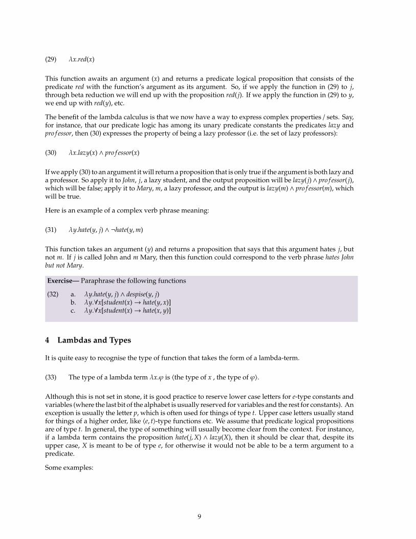
Exercise— Paraphrase the following functions
(32) a. λy.hate(y, j) ∧ despise(y, j)b. λy.∀x[student(x)→ hate(y, x)]c. λy.∀x[student(x)→ hate(x, y)]
4 Lambdas and Types
It is quite easy to recognise the type of function that takes the form of a lambda-term.
(33) The type of a lambda term λx.ϕ is 〈the type of x , the type of ϕ〉.
Although this is not set in stone, it is good practice to reserve lower case letters for e-type constants andvariables (where the last bit of the alphabet is usually reserved for variables and the rest for constants). Anexception is usually the letter p, which is often used for things of type t. Upper case letters usually standfor things of a higher order, like 〈e, t〉-type functions etc. We assume that predicate logical propositionsare of type t. In general, the type of something will usually become clear from the context. For instance,if a lambda term contains the proposition hate( j,X) ∧ lazy(X), then it should be clear that, despite itsupper case, X is meant to be of type e, for otherwise it would not be able to be a term argument to apredicate.
Some examples:
9
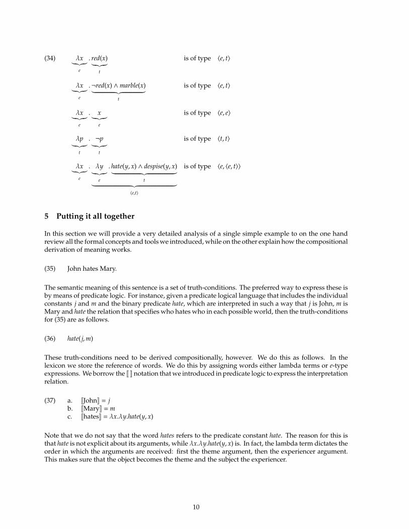
(34) λx︸︷︷︸e
. red(x)︸︷︷︸t
is of type 〈e, t〉
λx︸︷︷︸e
.¬red(x) ∧marble(x)︸ ︷︷ ︸t
is of type 〈e, t〉
λx︸︷︷︸e
. x︸︷︷︸e
is of type 〈e, e〉
λp︸︷︷︸t
. ¬p︸︷︷︸t
is of type 〈t, t〉
λx︸︷︷︸e
. λy︸︷︷︸e
. hate(y, x) ∧ despise(y, x)︸ ︷︷ ︸t︸ ︷︷ ︸
〈e,t〉
is of type 〈e, 〈e, t〉〉
5 Putting it all together
In this section we will provide a very detailed analysis of a single simple example to on the one handreview all the formal concepts and tools we introduced, while on the other explain how the compositionalderivation of meaning works.
(35) John hates Mary.
The semantic meaning of this sentence is a set of truth-conditions. The preferred way to express these isby means of predicate logic. For instance, given a predicate logical language that includes the individualconstants j and m and the binary predicate hate, which are interpreted in such a way that j is John, m isMary and hate the relation that specifies who hates who in each possible world, then the truth-conditionsfor (35) are as follows.
(36) hate( j,m)
These truth-conditions need to be derived compositionally, however. We do this as follows. In thelexicon we store the reference of words. We do this by assigning words either lambda terms or e-typeexpressions. We borrow the J K notation that we introduced in predicate logic to express the interpretationrelation.
(37) a. JJohnK = jb. JMaryK = mc. JhatesK = λx.λy.hate(y, x)
Note that we do not say that the word hates refers to the predicate constant hate. The reason for this isthat hate is not explicit about its arguments, while λx.λy.hate(y, x) is. In fact, the lambda term dictates theorder in which the arguments are received: first the theme argument, then the experiencer argument.This makes sure that the object becomes the theme and the subject the experiencer.
10
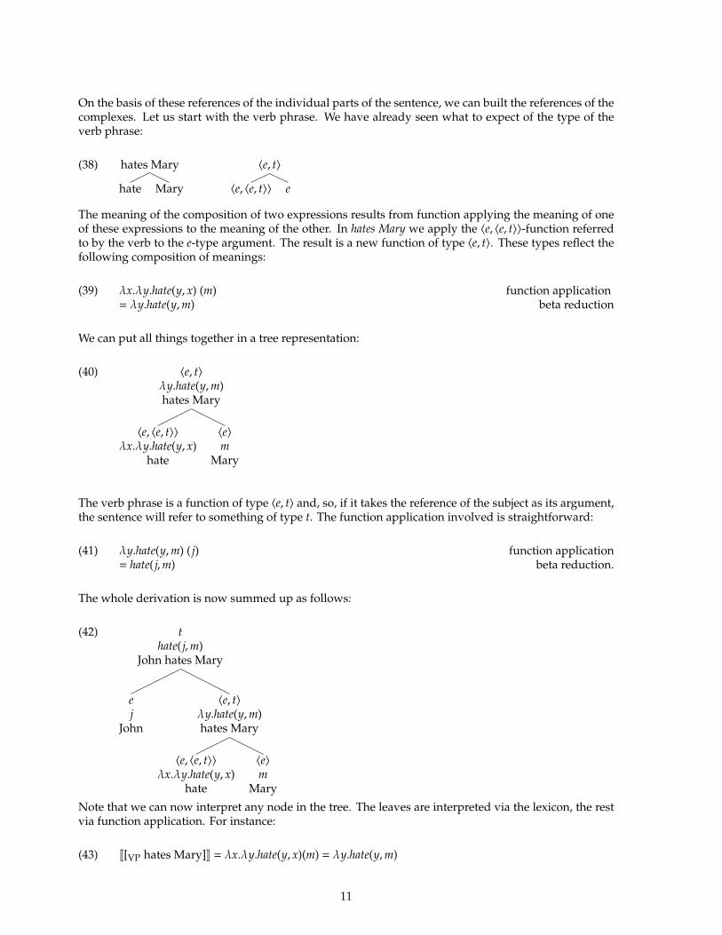
On the basis of these references of the individual parts of the sentence, we can built the references of thecomplexes. Let us start with the verb phrase. We have already seen what to expect of the type of theverb phrase:
(38) hates Mary
hate Mary
〈e, t〉
〈e, 〈e, t〉〉 e
The meaning of the composition of two expressions results from function applying the meaning of oneof these expressions to the meaning of the other. In hates Mary we apply the 〈e, 〈e, t〉〉-function referredto by the verb to the e-type argument. The result is a new function of type 〈e, t〉. These types reflect thefollowing composition of meanings:
(39) λx.λy.hate(y, x) (m) function application= λy.hate(y,m) beta reduction
We can put all things together in a tree representation:
(40) 〈e, t〉λy.hate(y,m)hates Mary
〈e, 〈e, t〉〉λx.λy.hate(y, x)
hate
〈e〉m
Mary
The verb phrase is a function of type 〈e, t〉 and, so, if it takes the reference of the subject as its argument,the sentence will refer to something of type t. The function application involved is straightforward:
(41) λy.hate(y,m) ( j) function application= hate( j,m) beta reduction.
The whole derivation is now summed up as follows:
(42) thate( j,m)
John hates Mary
ej
John
〈e, t〉λy.hate(y,m)hates Mary
〈e, 〈e, t〉〉λx.λy.hate(y, x)
hate
〈e〉m
Mary
Note that we can now interpret any node in the tree. The leaves are interpreted via the lexicon, the restvia function application. For instance:
(43) J[VP hates Mary]K = λx.λy.hate(y, x)(m) = λy.hate(y,m)
11
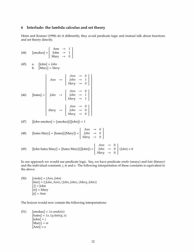
6 Interlude: the lambda calculus and set theory
Heim and Kratzer (1998) do it differently, they avoid predicate logic and instead talk about functionsand set theory directly.
(44) JsmokesK =
Ann → 1John → 1
Mary → 0
(45) a. JJohnK = John
b. JMaryK = Mary
(46) JhatesK =
Ann →
Ann → 0John → 1
Mary → 0
John →
Ann → 0John → 1
Mary → 1
Mary →
Ann → 0John → 0
Mary → 0
(47) JJohn smokesK = JsmokesK(JJohnK) = 1
(48) Jhates MaryK = JhatesK(JMaryK) =
Ann → 0John → 0
Mary → 0
(49) JJohn hates MaryK = Jhates MaryK(JJohnK) =
Ann → 0John → 0
Mary → 0
(John) = 0
In our approach we would use predicate logic. Say, we have predicate smoke (unary) and hate (binary)and the individual constants j, m and a. The following interpretation of these constants is equivalent tothe above.
(50) JsmokeK = {Ann, John}JhateK = {〈John,Ann〉, 〈John, John〉, 〈Mary, John〉}J jK = JohnJmK = MaryJaK = Ann
The lexicon would now contain the following interpretations:
(51) JsmokesK = λx.smoke(x)JhatesK = λx.λy.hate(y, x)JJohnK = jJMaryK = mJAnnK = a
12
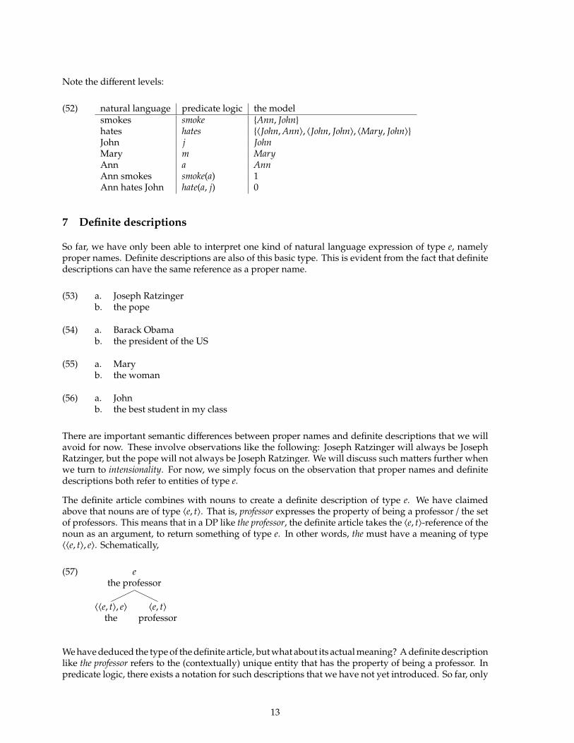
Note the different levels:
(52) natural language predicate logic the modelsmokes smoke {Ann, John}hates hates {〈John,Ann〉, 〈John, John〉, 〈Mary, John〉}John j JohnMary m MaryAnn a AnnAnn smokes smoke(a) 1Ann hates John hate(a, j) 0
7 Definite descriptions
So far, we have only been able to interpret one kind of natural language expression of type e, namelyproper names. Definite descriptions are also of this basic type. This is evident from the fact that definitedescriptions can have the same reference as a proper name.
(53) a. Joseph Ratzingerb. the pope
(54) a. Barack Obamab. the president of the US
(55) a. Maryb. the woman
(56) a. Johnb. the best student in my class
There are important semantic differences between proper names and definite descriptions that we willavoid for now. These involve observations like the following: Joseph Ratzinger will always be JosephRatzinger, but the pope will not always be Joseph Ratzinger. We will discuss such matters further whenwe turn to intensionality. For now, we simply focus on the observation that proper names and definitedescriptions both refer to entities of type e.
The definite article combines with nouns to create a definite description of type e. We have claimedabove that nouns are of type 〈e, t〉. That is, professor expresses the property of being a professor / the setof professors. This means that in a DP like the professor, the definite article takes the 〈e, t〉-reference of thenoun as an argument, to return something of type e. In other words, the must have a meaning of type〈〈e, t〉, e〉. Schematically,
(57) ethe professor
〈〈e, t〉, e〉the
〈e, t〉professor
We have deduced the type of the definite article, but what about its actual meaning? A definite descriptionlike the professor refers to the (contextually) unique entity that has the property of being a professor. Inpredicate logic, there exists a notation for such descriptions that we have not yet introduced. So far, only
13
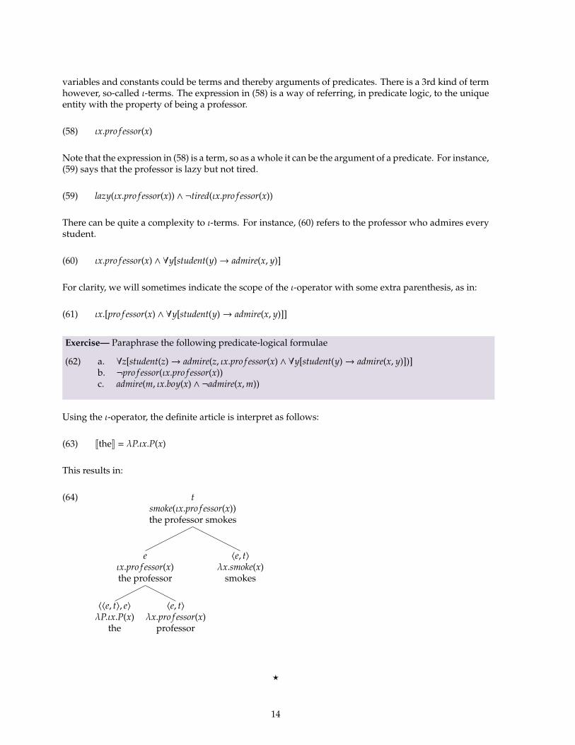
variables and constants could be terms and thereby arguments of predicates. There is a 3rd kind of termhowever, so-called ι-terms. The expression in (58) is a way of referring, in predicate logic, to the uniqueentity with the property of being a professor.
(58) ιx.pro f essor(x)
Note that the expression in (58) is a term, so as a whole it can be the argument of a predicate. For instance,(59) says that the professor is lazy but not tired.
(59) lazy(ιx.pro f essor(x)) ∧ ¬tired(ιx.pro f essor(x))
There can be quite a complexity to ι-terms. For instance, (60) refers to the professor who admires everystudent.
(60) ιx.pro f essor(x) ∧ ∀y[student(y)→ admire(x, y)]
For clarity, we will sometimes indicate the scope of the ι-operator with some extra parenthesis, as in:
(61) ιx.[pro f essor(x) ∧ ∀y[student(y)→ admire(x, y)]]
Exercise— Paraphrase the following predicate-logical formulae
(62) a. ∀z[student(z)→ admire(z, ιx.pro f essor(x) ∧ ∀y[student(y)→ admire(x, y)])]b. ¬pro f essor(ιx.pro f essor(x))c. admire(m, ιx.boy(x) ∧ ¬admire(x,m))
Using the ι-operator, the definite article is interpret as follows:
(63) JtheK = λP.ιx.P(x)
This results in:
(64) tsmoke(ιx.pro f essor(x))the professor smokes
eιx.pro f essor(x)the professor
〈〈e, t〉, e〉λP.ιx.P(x)
the
〈e, t〉λx.pro f essor(x)
professor
〈e, t〉λx.smoke(x)
smokes
?
14
We end this handout with two analyses from the Heim and Kratzer text book that have become especiallypopular, and which introduce some particularities of the composition process. (In what follows, we stickwith our approach involving predicate logic, however.)
See Heim and Kratzer 1998 chapters 1–5.
?
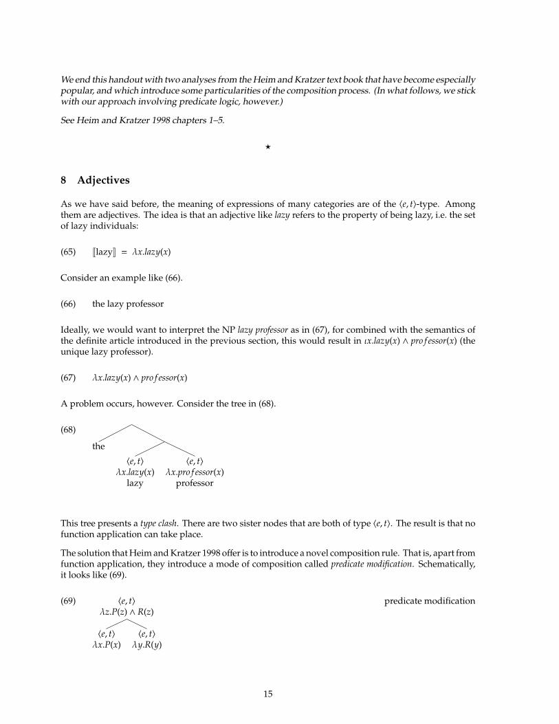
8 Adjectives
As we have said before, the meaning of expressions of many categories are of the 〈e, t〉-type. Amongthem are adjectives. The idea is that an adjective like lazy refers to the property of being lazy, i.e. the setof lazy individuals:
(65) JlazyK = λx.lazy(x)
Consider an example like (66).
(66) the lazy professor
Ideally, we would want to interpret the NP lazy professor as in (67), for combined with the semantics ofthe definite article introduced in the previous section, this would result in ιx.lazy(x) ∧ pro f essor(x) (theunique lazy professor).
(67) λx.lazy(x) ∧ pro f essor(x)
A problem occurs, however. Consider the tree in (68).
(68)
the
〈e, t〉λx.lazy(x)
lazy
〈e, t〉λx.pro f essor(x)
professor
This tree presents a type clash. There are two sister nodes that are both of type 〈e, t〉. The result is that nofunction application can take place.
The solution that Heim and Kratzer 1998 offer is to introduce a novel composition rule. That is, apart fromfunction application, they introduce a mode of composition called predicate modification. Schematically,it looks like (69).
(69) 〈e, t〉λz.P(z) ∧ R(z)
〈e, t〉λx.P(x)
〈e, t〉λy.R(y)
predicate modification
15
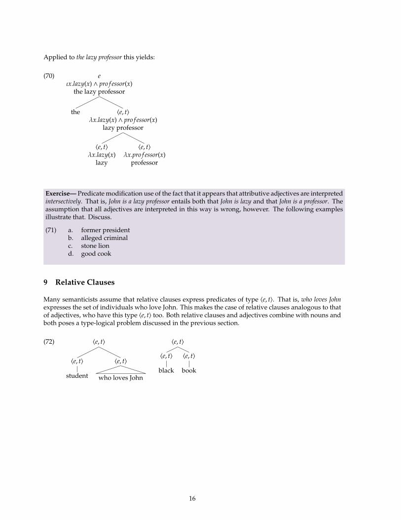
Applied to the lazy professor this yields:
(70) eιx.lazy(x) ∧ pro f essor(x)
the lazy professor
the 〈e, t〉λx.lazy(x) ∧ pro f essor(x)
lazy professor
〈e, t〉λx.lazy(x)
lazy
〈e, t〉λx.pro f essor(x)
professor
Exercise— Predicate modification use of the fact that it appears that attributive adjectives are interpretedintersectively. That is, John is a lazy professor entails both that John is lazy and that John is a professor. Theassumption that all adjectives are interpreted in this way is wrong, however. The following examplesillustrate that. Discuss.
(71) a. former presidentb. alleged criminalc. stone liond. good cook
9 Relative Clauses
Many semanticists assume that relative clauses express predicates of type 〈e, t〉. That is, who loves Johnexpresses the set of individuals who love John. This makes the case of relative clauses analogous to thatof adjectives, who have this type 〈e, t〉 too. Both relative clauses and adjectives combine with nouns andboth poses a type-logical problem discussed in the previous section.
(72) 〈e, t〉
〈e, t〉
student
〈e, t〉
who loves John
〈e, t〉
〈e, t〉
black
〈e, t〉
book
16
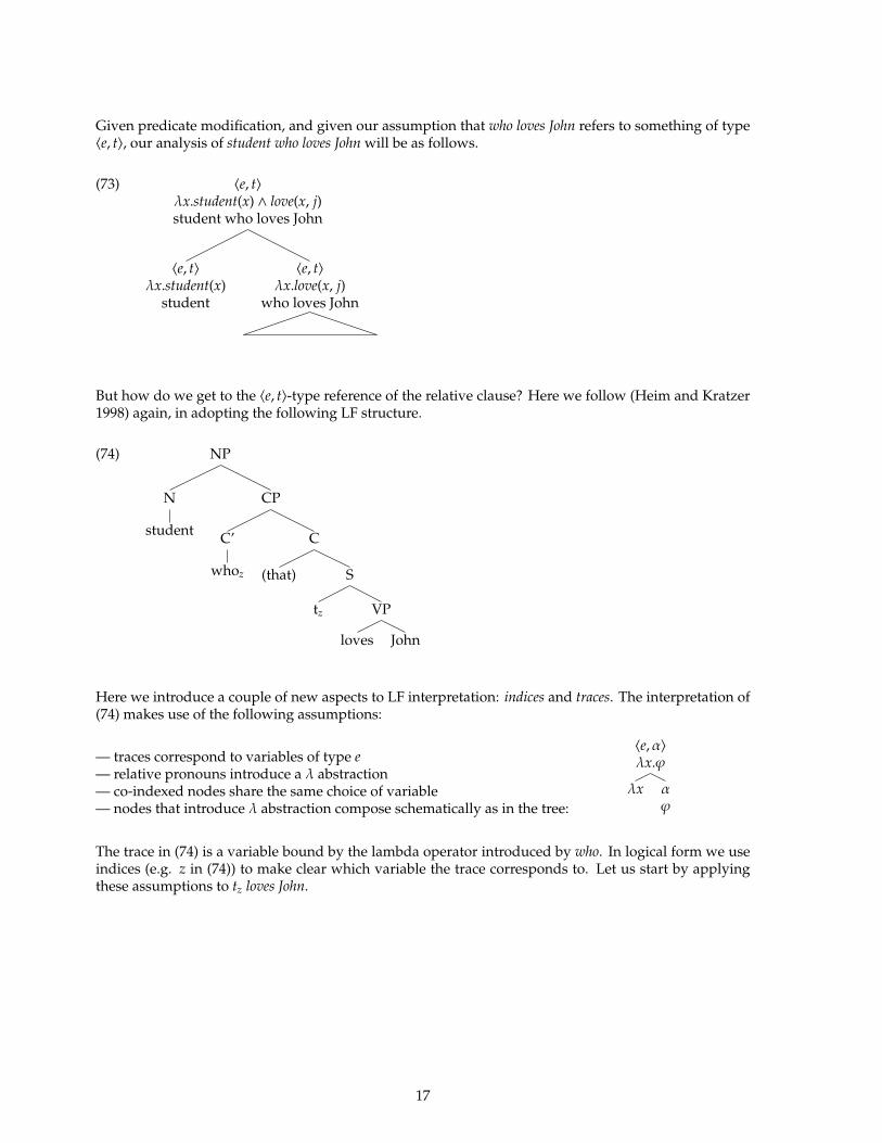
Given predicate modification, and given our assumption that who loves John refers to something of type〈e, t〉, our analysis of student who loves John will be as follows.
(73) 〈e, t〉λx.student(x) ∧ love(x, j)student who loves John
〈e, t〉λx.student(x)
student
〈e, t〉λx.love(x, j)
who loves John
But how do we get to the 〈e, t〉-type reference of the relative clause? Here we follow (Heim and Kratzer1998) again, in adopting the following LF structure.
(74) NP
N
student
CP
C’
whoz
C
(that) S
tz VP
loves John
Here we introduce a couple of new aspects to LF interpretation: indices and traces. The interpretation of(74) makes use of the following assumptions:
— traces correspond to variables of type e— relative pronouns introduce a λ abstraction— co-indexed nodes share the same choice of variable— nodes that introduce λ abstraction compose schematically as in the tree:
〈e, α〉λx.ϕ
λx αϕ
The trace in (74) is a variable bound by the lambda operator introduced by who. In logical form we useindices (e.g. z in (74)) to make clear which variable the trace corresponds to. Let us start by applyingthese assumptions to tz loves John.
17
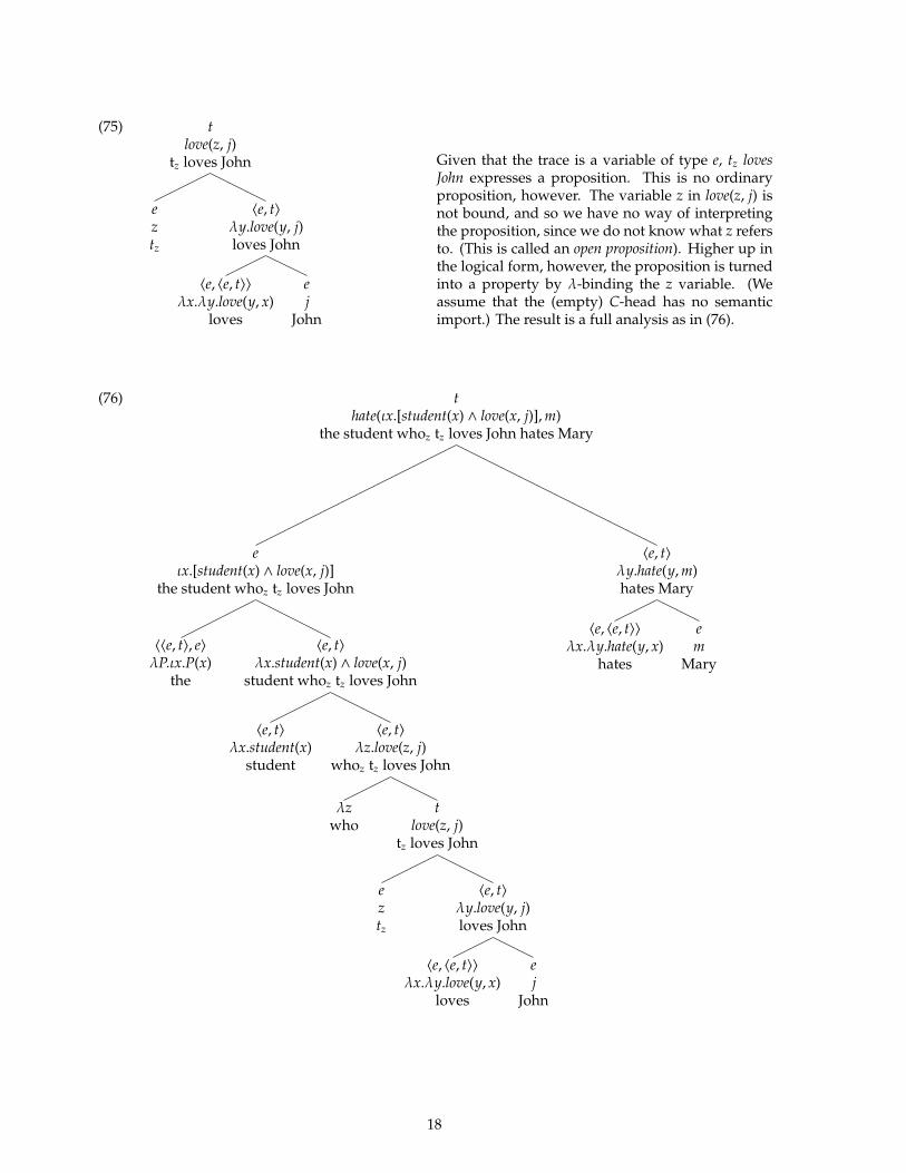
(75) tlove(z, j)
tz loves John
eztz
〈e, t〉λy.love(y, j)loves John
〈e, 〈e, t〉〉λx.λy.love(y, x)
loves
ej
John
Given that the trace is a variable of type e, tz lovesJohn expresses a proposition. This is no ordinaryproposition, however. The variable z in love(z, j) isnot bound, and so we have no way of interpretingthe proposition, since we do not know what z refersto. (This is called an open proposition). Higher up inthe logical form, however, the proposition is turnedinto a property by λ-binding the z variable. (Weassume that the (empty) C-head has no semanticimport.) The result is a full analysis as in (76).
(76) thate(ιx.[student(x) ∧ love(x, j)],m)
the student whoz tz loves John hates Mary
eιx.[student(x) ∧ love(x, j)]
the student whoz tz loves John
〈〈e, t〉, e〉λP.ιx.P(x)
the
〈e, t〉λx.student(x) ∧ love(x, j)
student whoz tz loves John
〈e, t〉λx.student(x)
student
〈e, t〉λz.love(z, j)
whoz tz loves John
λzwho
tlove(z, j)
tz loves John
eztz
〈e, t〉λy.love(y, j)loves John
〈e, 〈e, t〉〉λx.λy.love(y, x)
loves
ej
John
〈e, t〉λy.hate(y,m)hates Mary
〈e, 〈e, t〉〉λx.λy.hate(y, x)
hates
em
Mary
18
10 Further reading
A good further introduction on types and lambdas can be found in two publicly available coursehandouts by Henriette de Swart:
http://www.let.uu.nl/∼Henriette.deSwart/personal/Classes/barcelona/typ.pdf
&
http://www.let.uu.nl/∼Henriette.deSwart/personal/Classes/barcelona/lambda.pdf
References
Heim, I. and A. Kratzer (1998). Semantics in Generative Grammar. Blackwell Publishing.
A Appendix: The horror of beta reduction
To the untrained eye, the implicit β-reduction steps in a semantic derivation will often appear to be anentirely random manipulation of variables. The only way to learn to fully grasp what is going on is topractice making such derivations and to make the β-reduction steps explicit. In this section, I will gothrough an example in great detail, and explain how beta reduction and variable choice works.
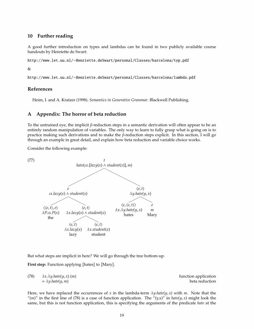
Consider the following example:
(77) thate(ιx.[lazy(x) ∧ student(x)],m)
eιx.lazy(x) ∧ student(x)
〈〈e, t〉, e〉λP.ιx.P(x)
the
〈e, t〉λx.lazy(x) ∧ student(x)
〈e, t〉λx.lazy(x)
lazy
〈e, t〉λx.student(x)
student
〈e, t〉λy.hate(y, x)
〈e, 〈e, t〉〉λx.λy.hate(y, x)
hates
em
Mary
But what steps are implicit in here? We will go through the tree bottom-up.
First step: Function applying JhatesK to JMaryK.
(78) λx.λy.hate(y, x) (m) function application= λy.hate(y,m) beta reduction
Here, we have replaced the occurrences of x in the lambda-term λy.hate(y, x) with m. Note that the“(m)” in the first line of (78) is a case of function application. The “(y,x)” in hate(y, x) might look thesame, but this is not function application, this is specifying the arguments of the predicate hate at the
19
predicate-logical level.
Notice that the order of the λ’s is the reverse of the order of the argument of the predicate hate. This isbecause in a derivation the object is processed first. In hate(y, x), it is the x variable that corresponds tothe object (the theme of the hate relation), and so the first argument to be filled in is x.
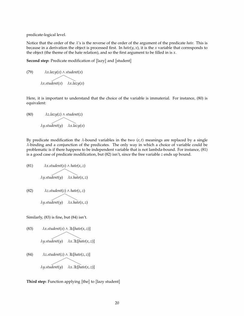
Second step: Predicate modification of JlazyK and JstudentK
(79) λx.lazy(x) ∧ student(x)
λx.student(x) λx.lazy(x)
Here, it is important to understand that the choice of the variable is immaterial. For instance, (80) isequivalent:
(80) λz.lazy(z) ∧ student(z)
λy.student(y) λx.lazy(x)
By predicate modification the λ-bound variables in the two 〈e, t〉 meanings are replaced by a singleλ-binding and a conjunction of the predicates. The only way in which a choice of variable could beproblematic is if there happens to be independent variable that is not lambda-bound. For instance, (81)is a good case of predicate modification, but (82) isn’t, since the free variable z ends up bound.
(81) λx.student(x) ∧ hate(x, z)
λy.student(y) λx.hate(x, z)
(82) λz.student(z) ∧ hate(z, z)
λy.student(y) λx.hate(x, z)
Similarly, (83) is fine, but (84) isn’t.
(83) λx.student(x) ∧ ∃z[hate(x, z)]
λy.student(y) λx.∃z[hate(x, z)]
(84) λz.student(z) ∧ ∃z[hate(z, z)]
λy.student(y) λx.∃z[hate(x, z)]
Third step: Function applying JtheK to Jlazy studentK
20
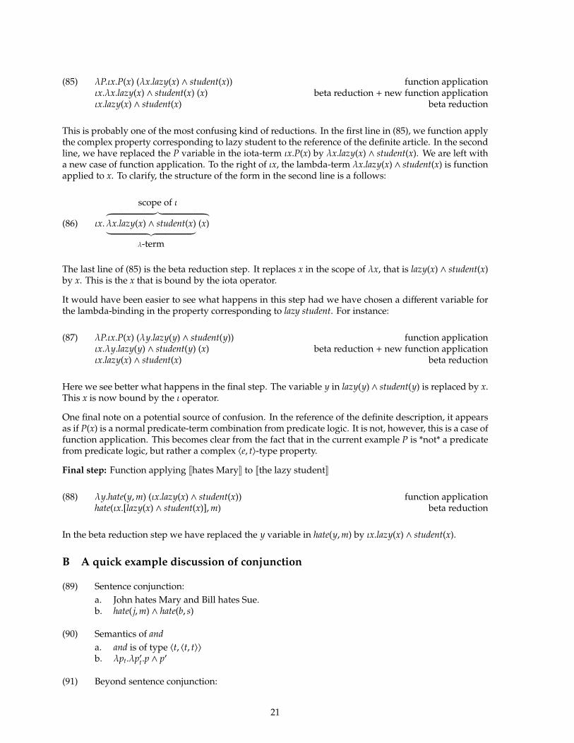
(85) λP.ιx.P(x) (λx.lazy(x) ∧ student(x)) function applicationιx.λx.lazy(x) ∧ student(x) (x) beta reduction + new function applicationιx.lazy(x) ∧ student(x) beta reduction
This is probably one of the most confusing kind of reductions. In the first line in (85), we function applythe complex property corresponding to lazy student to the reference of the definite article. In the secondline, we have replaced the P variable in the iota-term ιx.P(x) by λx.lazy(x) ∧ student(x). We are left witha new case of function application. To the right of ιx, the lambda-term λx.lazy(x) ∧ student(x) is functionapplied to x. To clarify, the structure of the form in the second line is a follows:
(86) ιx.
scope of ι︷ ︸︸ ︷λx.lazy(x) ∧ student(x)︸ ︷︷ ︸
λ-term
(x)
The last line of (85) is the beta reduction step. It replaces x in the scope of λx, that is lazy(x) ∧ student(x)by x. This is the x that is bound by the iota operator.
It would have been easier to see what happens in this step had we have chosen a different variable forthe lambda-binding in the property corresponding to lazy student. For instance:
(87) λP.ιx.P(x) (λy.lazy(y) ∧ student(y)) function applicationιx.λy.lazy(y) ∧ student(y) (x) beta reduction + new function applicationιx.lazy(x) ∧ student(x) beta reduction
Here we see better what happens in the final step. The variable y in lazy(y)∧ student(y) is replaced by x.This x is now bound by the ι operator.
One final note on a potential source of confusion. In the reference of the definite description, it appearsas if P(x) is a normal predicate-term combination from predicate logic. It is not, however, this is a case offunction application. This becomes clear from the fact that in the current example P is *not* a predicatefrom predicate logic, but rather a complex 〈e, t〉-type property.
Final step: Function applying Jhates MaryK to Jthe lazy studentK
(88) λy.hate(y,m) (ιx.lazy(x) ∧ student(x)) function applicationhate(ιx.[lazy(x) ∧ student(x)],m) beta reduction
In the beta reduction step we have replaced the y variable in hate(y,m) by ιx.lazy(x) ∧ student(x).
B A quick example discussion of conjunction
(89) Sentence conjunction:a. John hates Mary and Bill hates Sue.b. hate( j,m) ∧ hate(b, s)
(90) Semantics of anda. and is of type 〈t, 〈t, t〉〉b. λpt.λp′t.p ∧ p′
(91) Beyond sentence conjunction:
21
a. John and Mary hate Sue.b. John hates Sue and Mary.
(92) Early accounts:a. John and Mary hate Sue{ John hates Sue and Mary hates Sueb. John hates Sue and Mary{ John hates Sue and John hates Mary
(93) Problem with rewrite account:Exactly two students hate Mary and Sue(consider the case where Mary is hated by the students Bill, John and Harry, and Sue ishated by the students Bill, Harry and Larry.)
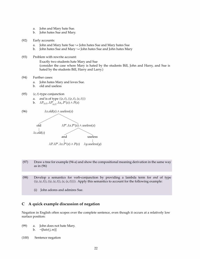
(94) Further cases:a. John hates Mary and loves Sue.b. old and useless
(95) 〈e, t〉-type conjunctiona. and is of type 〈〈e, t〉, 〈〈e, t〉, 〈e, t〉〉〉b. λP〈e,t〉.λP′
〈e,t〉.λxe.P′(x) ∧ P(x)
(96) λx.old(x) ∧ useless(x)
old
λz.old(z)
λP′.λx.P′(x) ∧ useless(x)
and
λP.λP′.λx.P′(x) ∧ P(x)
useless
λy.useless(y)
(97) Draw a tree for example (94-a) and show the compositional meaning derivation in the same wayas in (96)
(98) Develop a semantics for verb-conjunction by providing a lambda term for and of type〈〈e, 〈e, t〉〉, 〈〈e, 〈e, t〉〉, 〈e, 〈e, t〉〉〉〉. Apply this semantics to account for the following example:
(i) John adores and admires Sue.
C A quick example discussion of negation
Negation in English often scopes over the complete sentence, even though it occurs at a relatively lowsurface position:
(99) a. John does not hate Mary.b. ¬[hate( j,m)]
(100) Sentence negation
22
a. not is of type 〈t, t〉b. λpt.¬p
Not all negation scopes over the main clause:
(101) a. My car is old but not uselessb. old(c) ∧ ¬useless(c)
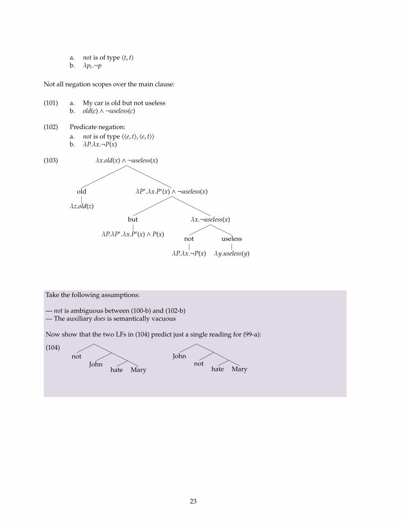
(102) Predicate negation:a. not is of type 〈〈e, t〉, 〈e, t〉〉b. λP.λx.¬P(x)
(103) λx.old(x) ∧ ¬useless(x)
old
λz.old(z)
λP′.λx.P′(x) ∧ ¬useless(x)
but
λP.λP′.λx.P′(x) ∧ P(x)
λx.¬useless(x)
not
λP.λx.¬P(x)
useless
λy.useless(y)
Take the following assumptions:
— not is ambiguous between (100-b) and (102-b)— The auxiliary does is semantically vacuous
Now show that the two LFs in (104) predict just a single reading for (99-a):
(104)not
Johnhate Mary
Johnnot
hate Mary
23