foundations of numerical analysisbraun/m426/textch1.pdf · chapter 1 introductory concepts it’s...
TRANSCRIPT

Foundations of Numerical Analysis
An Introduction using MATLAB
Tobin A. Driscoll and Richard J. BraunSeptember 3, 2008
Copyright c© 2008 by T.A. Driscoll and R.J. Braun. All rights reserved.Please do not redistribute for free or for profit.

ii
Contents
1 Introductory concepts 1
1.1 Mathematical background . . . . . . . . . . . . . . . . . . . . . . . . . . . . . . . . . . 1
1.2 Uses and types of computation . . . . . . . . . . . . . . . . . . . . . . . . . . . . . . . 3
1.3 Algorithms . . . . . . . . . . . . . . . . . . . . . . . . . . . . . . . . . . . . . . . . . . . 4
1.4 Errors . . . . . . . . . . . . . . . . . . . . . . . . . . . . . . . . . . . . . . . . . . . . . . 10
1.5 Conditioning . . . . . . . . . . . . . . . . . . . . . . . . . . . . . . . . . . . . . . . . . . 14
1.6 Stability: A case study . . . . . . . . . . . . . . . . . . . . . . . . . . . . . . . . . . . . 17
2 Square linear systems 23
2.1 Background in linear algebra . . . . . . . . . . . . . . . . . . . . . . . . . . . . . . . . 23
2.2 Triangular linear systems . . . . . . . . . . . . . . . . . . . . . . . . . . . . . . . . . . . 28
2.3 Gaussian elimination and LU factorization . . . . . . . . . . . . . . . . . . . . . . . . 31
2.4 Operation counts . . . . . . . . . . . . . . . . . . . . . . . . . . . . . . . . . . . . . . . 36
2.5 Row pivoting . . . . . . . . . . . . . . . . . . . . . . . . . . . . . . . . . . . . . . . . . 39
2.6 Vector and matrix norms . . . . . . . . . . . . . . . . . . . . . . . . . . . . . . . . . . . 45
2.7 Conditioning and stability for linear systems . . . . . . . . . . . . . . . . . . . . . . . 50
2.8 Special types of matrices . . . . . . . . . . . . . . . . . . . . . . . . . . . . . . . . . . . 55
3 Overdetermined linear systems 59
3.1 Linear least-squares problems and data fitting . . . . . . . . . . . . . . . . . . . . . . 59
3.2 The normal equations and orthogonality . . . . . . . . . . . . . . . . . . . . . . . . . . 62
3.3 QR factorization . . . . . . . . . . . . . . . . . . . . . . . . . . . . . . . . . . . . . . . . 67
3.4 Conditioning and stability for least squares . . . . . . . . . . . . . . . . . . . . . . . . 73
4 Matrix eigenvalues and eigenvectors 75
4.1 Background in eigenvalues . . . . . . . . . . . . . . . . . . . . . . . . . . . . . . . . . 75
4.2 Conditioning and the Schur decomposition . . . . . . . . . . . . . . . . . . . . . . . . 79
4.3 The QR iteration . . . . . . . . . . . . . . . . . . . . . . . . . . . . . . . . . . . . . . . . 83
4.4 Shifting and deflation . . . . . . . . . . . . . . . . . . . . . . . . . . . . . . . . . . . . . 86
4.5 Hessenberg reduction . . . . . . . . . . . . . . . . . . . . . . . . . . . . . . . . . . . . . 89
4.6 The singular value decomposition . . . . . . . . . . . . . . . . . . . . . . . . . . . . . 91
iii
iv CONTENTS
5 Iterative methods in linear algebra 97
5.1 Sparse matrices and fill-in . . . . . . . . . . . . . . . . . . . . . . . . . . . . . . . . . . 98
5.2 Power and inverse iteration . . . . . . . . . . . . . . . . . . . . . . . . . . . . . . . . . 102
5.3 Krylov subspaces and the Arnoldi iteration . . . . . . . . . . . . . . . . . . . . . . . . 108
5.4 Applications of the Arnoldi iteration . . . . . . . . . . . . . . . . . . . . . . . . . . . . 117
5.5 Practical considerations for linear systems . . . . . . . . . . . . . . . . . . . . . . . . . 126
6 Roots of nonlinear equations 139
6.1 Newton’s method . . . . . . . . . . . . . . . . . . . . . . . . . . . . . . . . . . . . . . . 139
6.2 Quasi-Newton methods . . . . . . . . . . . . . . . . . . . . . . . . . . . . . . . . . . . 146
6.3 Bracketing methods . . . . . . . . . . . . . . . . . . . . . . . . . . . . . . . . . . . . . . 151
6.4 Fixed point iteration . . . . . . . . . . . . . . . . . . . . . . . . . . . . . . . . . . . . . 156
6.5 Systems of nonlinear equations . . . . . . . . . . . . . . . . . . . . . . . . . . . . . . . 161
6.6 Methods for systems of equations . . . . . . . . . . . . . . . . . . . . . . . . . . . . . . 164
6.7 Summary . . . . . . . . . . . . . . . . . . . . . . . . . . . . . . . . . . . . . . . . . . . . 168
7 Interpolation 171
7.1 Piecewise linear interpolation . . . . . . . . . . . . . . . . . . . . . . . . . . . . . . . . 172
7.2 Cubic splines . . . . . . . . . . . . . . . . . . . . . . . . . . . . . . . . . . . . . . . . . . 178
7.3 B-splines . . . . . . . . . . . . . . . . . . . . . . . . . . . . . . . . . . . . . . . . . . . . 182
7.4 Interpolation by polynomials . . . . . . . . . . . . . . . . . . . . . . . . . . . . . . . . 190
Problems . . . . . . . . . . . . . . . . . . . . . . . . . . . . . . . . . . . . . . . . . . . . 195
7.5 The barycentric formulas . . . . . . . . . . . . . . . . . . . . . . . . . . . . . . . . . . . 195
7.6 The effects of node locations . . . . . . . . . . . . . . . . . . . . . . . . . . . . . . . . . 201
7.7 Chebyshev polynomials . . . . . . . . . . . . . . . . . . . . . . . . . . . . . . . . . . . 206
7.8 Trigonometric interpolation . . . . . . . . . . . . . . . . . . . . . . . . . . . . . . . . . 208
7.9 Approximation versus interpolation . . . . . . . . . . . . . . . . . . . . . . . . . . . . 213
7.10 Interpolation and approximation in MATLAB . . . . . . . . . . . . . . . . . . . . . . . 214
Problems . . . . . . . . . . . . . . . . . . . . . . . . . . . . . . . . . . . . . . . . . . . . 217
7.11 Parameterization of curves . . . . . . . . . . . . . . . . . . . . . . . . . . . . . . . . . . 219
Problems . . . . . . . . . . . . . . . . . . . . . . . . . . . . . . . . . . . . . . . . . . . . 222
8 Calculus 223
8.1 Simple finite differences . . . . . . . . . . . . . . . . . . . . . . . . . . . . . . . . . . . 223
8.2 General finite differences . . . . . . . . . . . . . . . . . . . . . . . . . . . . . . . . . . . 229
8.3 Newton–Cotes quadrature rules . . . . . . . . . . . . . . . . . . . . . . . . . . . . . . 233
Problems . . . . . . . . . . . . . . . . . . . . . . . . . . . . . . . . . . . . . . . . . . . . 239
8.4 Adaptive quadrature . . . . . . . . . . . . . . . . . . . . . . . . . . . . . . . . . . . . . 239
8.5 Clenshaw–Curtis and Gaussian quadrature . . . . . . . . . . . . . . . . . . . . . . . . 244
Problems . . . . . . . . . . . . . . . . . . . . . . . . . . . . . . . . . . . . . . . . . . . . 252
8.6 Orthogonal polynomials . . . . . . . . . . . . . . . . . . . . . . . . . . . . . . . . . . . 253
8.7 Improper integrals and singularities . . . . . . . . . . . . . . . . . . . . . . . . . . . . 256
8.8 Multidimensional integrals . . . . . . . . . . . . . . . . . . . . . . . . . . . . . . . . . 261

CONTENTS v
9 Initial-value problems for ODE 265
9.1 Background theory . . . . . . . . . . . . . . . . . . . . . . . . . . . . . . . . . . . . . . 2659.2 Euler’s method . . . . . . . . . . . . . . . . . . . . . . . . . . . . . . . . . . . . . . . . 2689.3 Convergence of one-step formulas . . . . . . . . . . . . . . . . . . . . . . . . . . . . . 2729.4 Systems of differential equations . . . . . . . . . . . . . . . . . . . . . . . . . . . . . . 2749.5 Runge–Kutta methods . . . . . . . . . . . . . . . . . . . . . . . . . . . . . . . . . . . . 2809.6 Adaptive step size and error control . . . . . . . . . . . . . . . . . . . . . . . . . . . . 2889.7 Multistep methods . . . . . . . . . . . . . . . . . . . . . . . . . . . . . . . . . . . . . . 2929.8 Implicit and predictor-corrector methods . . . . . . . . . . . . . . . . . . . . . . . . . 3029.9 Stability and convergence of multistep methods . . . . . . . . . . . . . . . . . . . . . 3079.10 Stability regions . . . . . . . . . . . . . . . . . . . . . . . . . . . . . . . . . . . . . . . . 3119.11 Linearization and model problems . . . . . . . . . . . . . . . . . . . . . . . . . . . . . 3189.12 Stiff systems . . . . . . . . . . . . . . . . . . . . . . . . . . . . . . . . . . . . . . . . . . 320
Further model problems . . . . . . . . . . . . . . . . . . . . . . . . . . . . . . . . . . . 322Implementation . . . . . . . . . . . . . . . . . . . . . . . . . . . . . . . . . . . . . . . . 323Wrapping up . . . . . . . . . . . . . . . . . . . . . . . . . . . . . . . . . . . . . . . . . . 326
9.13 MATLAB’s built-in IVP solvers . . . . . . . . . . . . . . . . . . . . . . . . . . . . . . . 3279.14 Summary . . . . . . . . . . . . . . . . . . . . . . . . . . . . . . . . . . . . . . . . . . . . 332
10 Boundary-value problems for ODE 335
10.1 Introduction . . . . . . . . . . . . . . . . . . . . . . . . . . . . . . . . . . . . . . . . . . 33510.2 Shooting . . . . . . . . . . . . . . . . . . . . . . . . . . . . . . . . . . . . . . . . . . . . 33710.3 Finite difference methods for the linear TPBVP . . . . . . . . . . . . . . . . . . . . . . 34210.4 Finite differences for nonlinear problems . . . . . . . . . . . . . . . . . . . . . . . . . 34910.5 The Galerkin method for the linear TPBVP . . . . . . . . . . . . . . . . . . . . . . . . 35210.6 Piecewise linear finite elements . . . . . . . . . . . . . . . . . . . . . . . . . . . . . . . 35610.7 BVPs in MATLAB . . . . . . . . . . . . . . . . . . . . . . . . . . . . . . . . . . . . . . . 361
11 Partial differential equations 367
11.1 Introduction . . . . . . . . . . . . . . . . . . . . . . . . . . . . . . . . . . . . . . . . . . 36711.2 Method of lines . . . . . . . . . . . . . . . . . . . . . . . . . . . . . . . . . . . . . . . . 37411.3 Accuracy and stability in the method of lines . . . . . . . . . . . . . . . . . . . . . . . 38111.4 Boundary conditions . . . . . . . . . . . . . . . . . . . . . . . . . . . . . . . . . . . . . 386
Neumann boundary conditions . . . . . . . . . . . . . . . . . . . . . . . . . . . . . . . 388Advection equation . . . . . . . . . . . . . . . . . . . . . . . . . . . . . . . . . . . . . . 388Nonlinear terms . . . . . . . . . . . . . . . . . . . . . . . . . . . . . . . . . . . . . . . . 390
11.5 Wave equation . . . . . . . . . . . . . . . . . . . . . . . . . . . . . . . . . . . . . . . . . 39111.6 Finite differences for Poisson’s equation . . . . . . . . . . . . . . . . . . . . . . . . . . 393

vi CONTENTS

Chapter 1
Introductory concepts
It’s all a lot of simple tricks and nonsense.
—Han Solo, Star Wars
One of the most important things to realize in computation—the thing that makes it intellectuallyexciting—is that methods which are mathematically equivalent may be vastly different in termsof computational performance. It often happens that the most obvious, direct, or well-knownmethod for a particular problem is unsuitable in computational practice. Hence in this book theemphasis is on the study of methods: how to find them, study their properties, and choose amongthem.
1.1 Mathematical background
Broadly speaking, you should be familiar with basic calculus (typically three college semesters)and linear algebra (half or one semester). For the chapters on differential equations, an introduc-tory course is recommended.
From linear algebra you should be comfortable with matrices, vectors, and simple algebra withthem (addition and multiplication). Hopefully you are familiar with their connection to linearsystems of the form Ax = b, and how to solve these systematically via Gaussian elimination.
From calculus we will use ideas such as limits, continuity and differentiability freely butmostly without rigor. The most important calculus topic you are likely to need refreshment onis the Taylor series. For a function f (x) near x = a, we have the two useful forms
f (x) = f (a) + (x − a) f ′(a) +1
2f ′′(a)(x − a)2 + · · · + 1
n!f (n)(a)(x − a)n + · · · (1.1a)
f (a + h) = f (a) + h f ′(a) +h2
2f ′′(a) + · · · + hn
n!f (n)(a) + · · · . (1.1b)
(The connection between the two forms is just x = a + h.) Such a series is always valid at least forx lying in an interval (a − R, a + R), where R may be zero or infinity. For values of x close to a (i.e.,
1

2 CHAPTER 1. INTRODUCTORY CONCEPTS
|h| small), we can truncate the series after a few terms and get a good approximating polynomial—polynomials as a class being much more agreeable than general functions! The effects of truncationcan sometimes be analyzed using the remainder form of the Taylor series,
f (a + h) = f (a) + h f ′(a) + · · · + 1
n!f (n)(a)hn +
1
(n + 1)!f (n+1)(ξ)hn+1, (1.2)
where ξ = ξ(h) is an unknowable number somewhere in the interval (0, h).One of the most important Taylor series is the geometric series,
1
1 − x= 1 + x + x2 + x3 + · · · , (1.3)
valid for all |x| < 1 only. It is the limit of the finite geometric sum
n
∑k=0
xk =1 − xn+1
1 − x. (1.4)
The geometric series can be generalized to the binomial series,
(1 + x)α = 1 + αx +α(α − 1)
2x2 + · · · + α · · · (α − n + 1)
n!xn + · · · . (1.5)
It also converges for |x| < 1, and it becomes a finite sum if α is a nonnegative integer. Anotherfundamental series is the exponential series,
ex = 1 + x +1
2x2 + · · · 1
n!xn + · · · , (1.6)
which is valid for all x.
Problems
1.1.1. Derive the first four nonzero terms of the Taylor series of the following functions about the givenpoints.
(a) cos(x), a = 0
(b) cos(x), a = π/2
(c) cosh(x), a = 0
(d) e−x2, a = 0 (Hint: Use (1.6).)
1.1.2. (a) Derive
log(1 + x) = x − x2
2+
x3
3− · · ·+ (−1)n−1 xn
n+ · · · , (1.7)
valid for |x| < 1.
(b) Derive
log
(
1 + y
1 − y
)
= 2y +2
3y3 +
2
5y5 +
2
7y7 + · · · , (1.8)
valid for |y| < 1.

1.2. USES AND TYPES OF COMPUTATION 3
1.2 Uses and types of computation
The topic of this book is computation for mathematically formulated problems. Our discussionexcludes other uses of computation, such as communications, data retrieval and mining, and vi-sualization, though these of course play important roles in science and engineering. Mathematicalcomputation is needed because the tools of mathematical analysis employed by humans, whileable to give many insights, cannot nearly answer all the questions we like to pose. Computers,able to perform arithmetic and logical operations trillions of times faster than we do, can be usedto produce additional insights.
One of the very first decisions you need to make before turning to a computer is whetheryou will use so-called symbolic or numerical methods. Symbolic computational environments(Maple, Mathematica, and Mathcad, for example) emphasize two particular abilities: understand-ing of abstract variables and expressions, such as
∫
xn dx; and the use of exact or arbitrarily accu-
rate numbers, such as π or√
2. These systems do mathematical manipulation much as you would,only much faster and more encyclopedically. Numerical environments (MATLAB, Fortran, C, andmost other compiled languages) operate natively on numerical values. The distinguishing featureof numerical computation is that noninteger real numbers are represented only approximately,and as a result arithmetic can be done only imprecisely.
It might seem puzzling that anyone would ever choose a system of imprecise arithmetic overan exact one. However, exact arithmetic demands much larger burdens of computer resourcesand time, and in many contexts there is no payoff for the extra costs.
As an example, consider the problem of finding the mth root of a number, A1/m. In principlesolving this problem takes an infinite number of the fundamental arithmetic operations +, −, ×,÷. There is a simple and ancient geometric algorithm for the case of square roots, m = 2. SupposeA > 0 is given and we have a guess x for
√A. We can imagine x as one side of a rectangle whose
area is A. Hence the other dimension of the rectangle is A/x. If these two lengths are identical(i. e., the rectangle is in fact a square), then their shared value is the square root, and we are done.Otherwise, we can easily show that the square root lies between x and A/x, so it seems reasonableto use the average of them as an improved guess. We represent this process with the formula
xn+1 =1
2
(
xn +A
xn
)
, n = 0, 1, 2, . . . . (1.9)
This formula represents an iteration. Given an initial guess x0 for√
A, we set n = 0 and get a(better?) guess x1. Then we set n = 1 and get x2, etc., until we are satisfied or give up.
For mth roots we can generalize this reasoning to an m-dimensional box of volume A whosesides are x, x, . . . , A/xm−1. In this case the averaging leads to
xn+1 =1
m
(
(m − 1)xn +A
xm−1n
)
, n = 0, 1, 2, . . . . (1.10)
Figure 1.1 shows the result of this iteration with m = 5 and A = 2. Although we are usingMaple, we have effectively put it into “numerical mode” by giving x an initial value with a decimalpoint in it. Hence all the results are rounded off to 15 significant digits. The iteration seems tobehave quite nicely. After five iterations it has found 10 digits accurately.
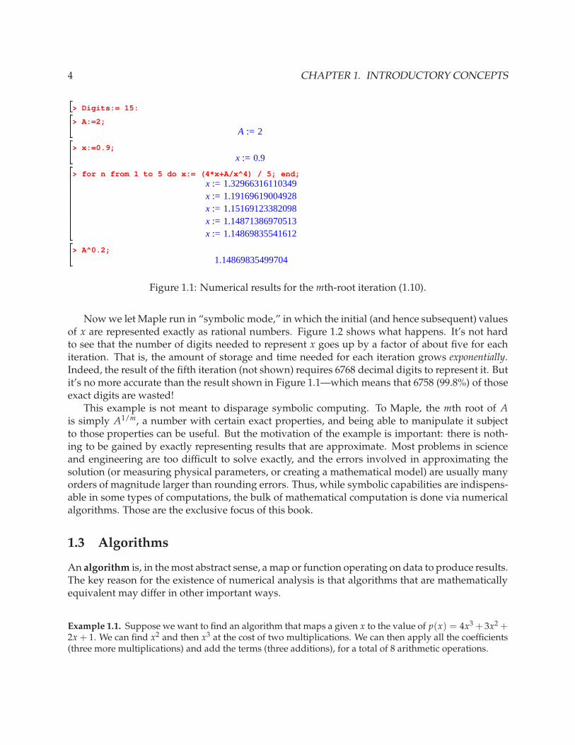
4 CHAPTER 1. INTRODUCTORY CONCEPTS
> Digits:= 15:
> A:=2;
A := 2
> x:=0.9;
x := 0.9
> for n from 1 to 5 do x:= (4*x+A/x^4) / 5; end;x := 1.32966316110349x := 1.19169619004928x := 1.15169123382098x := 1.14871386970513x := 1.14869835541612
> A^0.2;
1.14869835499704
Figure 1.1: Numerical results for the mth-root iteration (1.10).
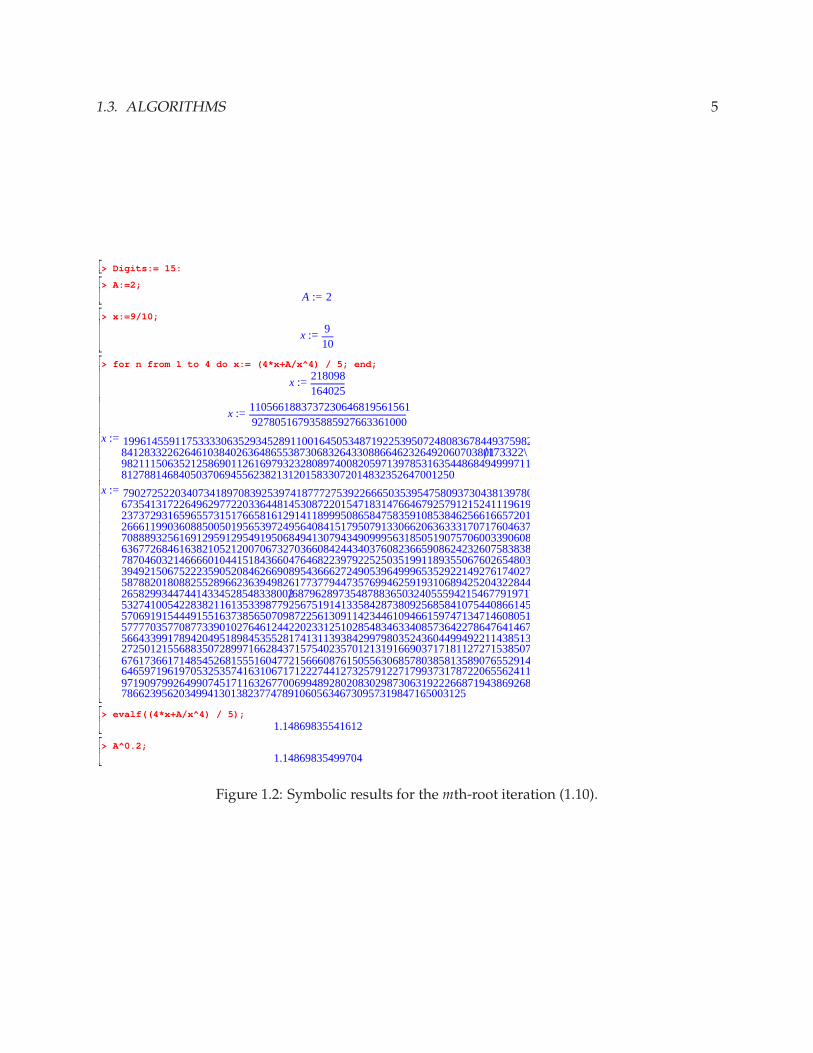
Now we let Maple run in “symbolic mode,” in which the initial (and hence subsequent) valuesof x are represented exactly as rational numbers. Figure 1.2 shows what happens. It’s not hardto see that the number of digits needed to represent x goes up by a factor of about five for eachiteration. That is, the amount of storage and time needed for each iteration grows exponentially.Indeed, the result of the fifth iteration (not shown) requires 6768 decimal digits to represent it. Butit’s no more accurate than the result shown in Figure 1.1—which means that 6758 (99.8%) of thoseexact digits are wasted!
This example is not meant to disparage symbolic computing. To Maple, the mth root of Ais simply A1/m, a number with certain exact properties, and being able to manipulate it subjectto those properties can be useful. But the motivation of the example is important: there is noth-ing to be gained by exactly representing results that are approximate. Most problems in scienceand engineering are too difficult to solve exactly, and the errors involved in approximating thesolution (or measuring physical parameters, or creating a mathematical model) are usually manyorders of magnitude larger than rounding errors. Thus, while symbolic capabilities are indispens-able in some types of computations, the bulk of mathematical computation is done via numericalalgorithms. Those are the exclusive focus of this book.
1.3 Algorithms
An algorithm is, in the most abstract sense, a map or function operating on data to produce results.The key reason for the existence of numerical analysis is that algorithms that are mathematicallyequivalent may differ in other important ways.
Example 1.1. Suppose we want to find an algorithm that maps a given x to the value of p(x) = 4x3 + 3x2 +2x + 1. We can find x2 and then x3 at the cost of two multiplications. We can then apply all the coefficients(three more multiplications) and add the terms (three additions), for a total of 8 arithmetic operations.
1.3. ALGORITHMS 5
> Digits:= 15:
> A:=2;
A := 2
> x:=9/10;
x := 910
> for n from 1 to 4 do x:= (4*x+A/x^4) / 5; end;
x := 218098164025
x := 1105661883737230646819561561927805167935885927663361000
x := 19961455911753333063529345289110016450534871922539507248083678449375982\84128332262646103840263648655387306832643308866462326492060703801173322\982111506352125869011261697932328089740082059713978531635448684949997112\8127881468405037069455623821312015833072014832352647001250
x := 79027252203407341897083925397418777275392266650353954758093730438139780\673541317226496297722033644814530872201547183147664679257912152411196195\237372931659655731517665816129141189995086584758359108538462566166572019\266611990360885005019565397249564084151795079133066206363331707176046374\708889325616912959129549195068494130794349099956318505190757060033906083\636772684616382105212007067327036608424434037608236659086242326075838380\787046032146666010441518436604764682239792252503519911893550676026548034\394921506752223590520846266908954366627249053964999653529221492761740277\587882018088255289662363949826177377944735769946259193106894252043228442\26582993447441433452854833800268796289735487883650324055594215467791971\532741005422838211613533987792567519141335842873809256858410754408661451\570691915444915516373856507098722561309114234461094661597471347146080514\577770357708773390102764612442202331251028548346334085736422786476414675\566433991789420495189845355281741311393842997980352436044994922114385136\272501215568835072899716628437157540235701213191669037171811272715385071\676173661714854526815551604772156660876150556306857803858135890765529140\646597196197053253574163106717122274412732579122717993731787220655624118\971909799264990745171163267700699489280208302987306319222668719438692684\786623956203499413013823774789106056346730957319847165003125
> evalf((4*x+A/x^4) / 5);
1.14869835541612
> A^0.2;
1.14869835499704
Figure 1.2: Symbolic results for the mth-root iteration (1.10).
6 CHAPTER 1. INTRODUCTORY CONCEPTS
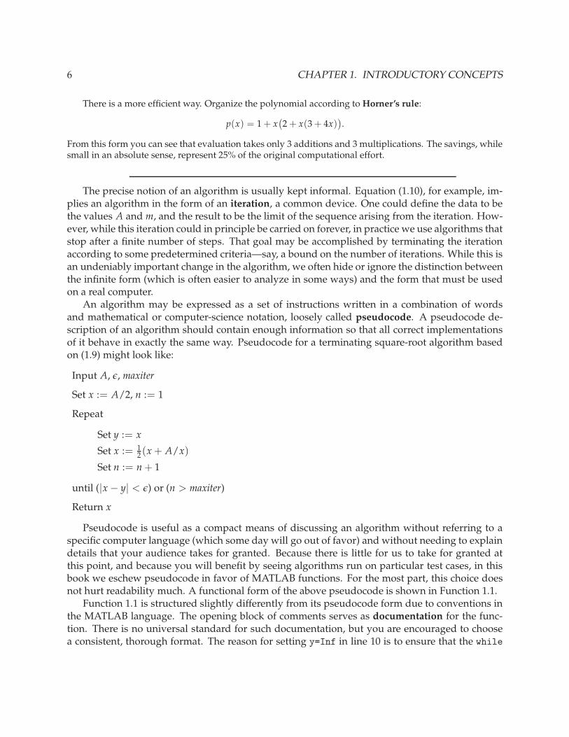
There is a more efficient way. Organize the polynomial according to Horner’s rule:
p(x) = 1 + x(
2 + x(3 + 4x))
.
From this form you can see that evaluation takes only 3 additions and 3 multiplications. The savings, whilesmall in an absolute sense, represent 25% of the original computational effort.
The precise notion of an algorithm is usually kept informal. Equation (1.10), for example, im-plies an algorithm in the form of an iteration, a common device. One could define the data to bethe values A and m, and the result to be the limit of the sequence arising from the iteration. How-ever, while this iteration could in principle be carried on forever, in practice we use algorithms thatstop after a finite number of steps. That goal may be accomplished by terminating the iterationaccording to some predetermined criteria—say, a bound on the number of iterations. While this isan undeniably important change in the algorithm, we often hide or ignore the distinction betweenthe infinite form (which is often easier to analyze in some ways) and the form that must be usedon a real computer.
An algorithm may be expressed as a set of instructions written in a combination of wordsand mathematical or computer-science notation, loosely called pseudocode. A pseudocode de-scription of an algorithm should contain enough information so that all correct implementationsof it behave in exactly the same way. Pseudocode for a terminating square-root algorithm basedon (1.9) might look like:
Input A, ǫ, maxiter
Set x := A/2, n := 1
Repeat
Set y := x
Set x := 12(x + A/x)
Set n := n + 1
until (|x − y| < ǫ) or (n > maxiter)
Return x
Pseudocode is useful as a compact means of discussing an algorithm without referring to aspecific computer language (which some day will go out of favor) and without needing to explaindetails that your audience takes for granted. Because there is little for us to take for granted atthis point, and because you will benefit by seeing algorithms run on particular test cases, in thisbook we eschew pseudocode in favor of MATLAB functions. For the most part, this choice doesnot hurt readability much. A functional form of the above pseudocode is shown in Function 1.1.
Function 1.1 is structured slightly differently from its pseudocode form due to conventions inthe MATLAB language. The opening block of comments serves as documentation for the func-tion. There is no universal standard for such documentation, but you are encouraged to choosea consistent, thorough format. The reason for setting y=Inf in line 10 is to ensure that the while

1.3. ALGORITHMS 7
Function 1.1 Iterative approximation of square roots.
1 function x = sqroot(A,tol)
2 % SQROOT Iterative approximation to the square root.
3 % Input:
4 % A Value to be rooted (scalar)
5 % tol Desired upper bound for the error in the result (scalar)
6 % Output:
7 % x An aproximation to sqrt(A) (scalar)
8
9 maxiter = 16;
10 x = A/2; y = Inf;
11 n = 1;
12 while abs(x-y) > tol
13 y = x;
14 x = (x+A/x)/2;
15 n = n+1;
16 if n > maxiter, warning(’Maximum iterations exceeded’), break, end
17 end
18
condition is initially true, so the loop body is executed at least once. Line 16 shows how functionscan display warnings to the user but still return output (after break exits the loop); an error com-mand would also display a message but halt execution and return no output as well. Appropriatewarnings and errors are very good programming practice, but we do not often include them inthis book in order to maintain our mathematical focus.
As another example, Function 1.2 implements an algorithm that applies Horner’s rule,
p(x) = c1xn + c2xn−1 + · · · + cnx + cn+1 =(
· · ·(
(c1x + c2)x + c3
)
x + · · · + cn
)
x + cn+1. (1.11)
In MATLAB, it is conventional to represent a polynomial by a vector of its coefficients in descend-ing order of degree. As you can see from Function 1.2, MATLAB deals with vectors very naturally:you can query the vector to find its length, and you can access the kth element of a vector c by typ-ing c(k). Like Function 1.1, Function 1.2 features an iteration. In this case, however, the number ofiterations is known before the iteration begins, and consequently we use a for construction ratherthan while as in Function 1.1.
The MATLAB codes in this section are not necessarily what an experienced MATLAB pro-grammer would write. MATLAB’s language has a number of features that can make certaintasks get expressed more compactly or generally than when using a more obvious syntax. Inthis book, however, we try to err on the side of clarity, using only a limited range of MATLAB’spower. As you will see, our MATLAB functions are still quite different (and simpler) than theequivalent functions you would write in a lower-level language like C or FORTRAN, or a moreobject-oriented language like Java.
MATLAB has a built-in function polyval that does essentially the same thing as our horner,so for good form we use polyval in the example below and the rest of the book.

8 CHAPTER 1. INTRODUCTORY CONCEPTS
Function 1.2 Evaluation of a polynomial by Horner’s rule.
1 function p = horner(c,x)
2 % HORNER Evaluate polynomial using Horner’s rule.
3 % Input:
4 % c Coefficients of polynomial, in descending order (vector)
5 % x Evaluation point (scalar)
6 % Output:
7 % p Value of the polynomial at x (scalar)
8
9 n = length(c);
10 p = c(1);
11 for k = 2:n+1
12 p = x*p + c(k);
13 end
Example 1.2. Taylor expansion (see problem 1.1.2) implies that
log(1 + x) = x − x2
2+
x3
3− · · ·+ (−1)n−1 xn
n+ · · · , (1.12)
which is valid for |x| < 1 and x = 1. Summing the series implies an infinite algorithm, but we can write aMATLAB function that returns the polynomial resulting by truncation to the first n terms of this series.
1 function f = logseries1(x,n)
2
3 c(1) = 0; % constant term (x^0)
4 for k = 1:n
5 c(k+1) = (-1)^(k+1)/k; % coeff of x^k
6 end
7 c = c(end:-1:1); % convert to descending order
8 f = polyval(c,x);
In this function we encounter a common problem: the way we want to subscript a vector mathematicallydoes not agree with MATLAB conventions. In line 5, for example, we must conform to the fact that vectorsare indexed starting at 1, never at 0. And in line 7, we compensate for MATLAB’s preference for descendingorder of degree in polynomial coefficients.
Applying our function for x = 1/2, we get
>> format long % to show all digits
>> log(1.5) % exact value
ans =
0.40546510810816
>> logseries1(0.5,5)
ans =

1.3. ALGORITHMS 9
0.40729166666667
>> logseries1(0.5,50)
ans =
0.40546510810816
In this case, 50 terms are sufficient to get a valid approximation for all available digits. In general practiceit might make more sense to select the truncation value of n automatically, based on x.
Constructing algorithms often involves balancing tradeoffs. Factors desired in an algorithmare
Stability If the inputs are changed by tiny amounts, the outputs should not be dramatically dif-ferent (unless the problem itself has this nature).
Reliability The algorithm should do what it claims and state its limitations.
Robustness The algorithm should be applicable to as broad a range of inputs as possible anddetect run-time failures.
Accuracy Errors should be as small as possible. Ideally one should be able to choose in advance anerror level that is then guaranteed by the method; more often we have to settle for asymptoticbounds on or estimates of the error.
Efficiency The algorithm should minimize the effort needed (say, execution time) to achieve agiven level of accuracy.
Storage The algorithm should require minimal memory resources.
Simplicity The algorithm should be as easy as possible to describe and program.
Also, remember that every algorithm solves only a mathematical problem. It cannot offer guid-ance on how well that problem models the true situation of interest, how well physical parametershave been measured, and so on. Always approach computer-generated results with healthy skep-ticism.
Problems
1.3.1. Modify Function 1.1 to find the mth root of a number using (1.10), where m is another input parameterfor the function. Be sure to test your function on a few cases.
1.3.2. There is an iteration to find the inverse of a nonzero value a using only multiplication and subtraction:
xn+1 = xn(2 − axn).
(a) Show that if xn+1 = xn = r (we say that r is a fixed point of the iteration), then either r = 0 orr = 1/a.
10 CHAPTER 1. INTRODUCTORY CONCEPTS
(b) Write a MATLAB function to implement this iteration. You will have to specify how to stop thealgorithm when |xn − a−1| ≤ ǫ, for an arbitrary ǫ, without doing any divisions or inversions.
1.3.3. In statistics, one defines the variance of sample values x1, . . . , xn by
s2 =1
n − 1
n
∑i=1
(xi − x)2, x =1
n
n
∑i=1
xi. (1.13)
Write a MATLAB function s2=samplevar(x) that takes as input a vector x of any length and returnss2 as calculated by the formula. You should test your function on some data and compare it toMATLAB’s built-in var.
1.4 Errors
In the two preceding sections we have seen that we will have to expect errors as a cost of doingnumerical business. We have a few different ways of measuring and talking about errors.
Suppose that x is an approximation to an exact result x∗. Three ways to measure the error in xare
Error x∗ − x Relative error|x∗ − x||x∗|
Absolute error |x∗ − x| Accurate digits
⌊
− log10
( |x∗ − x||x∗|
)⌋
The terms “error” and “absolute error” are often used interchangeably. To define accurate digitswe have used the floor function ⌊t⌋, which gives the largest integer no greater than t. Digitscorrespond to the notion of significant digits in science, and are also linked to scientific notation;e. g., 6.02 × 10⁻²³ is given to 25 decimal places but just three digits.
We have assumed in our definitions that x and x∗ are numbers. If they are vectors, functions,etc., we need a definition of magnitude or norm to replace the absolute values. (Sometimes normsare written using the same symbol.)
The two previous sections have introduced two unavoidable sources of error for correctly im-plemented numerical algorithms: roundoff error, due to approximating infinitely long numbers,and truncation error, due to approximating infinitely long algorithms. Almost all of the time,truncation error is far more important than roundoff error.
Roundoff error
We cannot represent the entire abstract continuum of real numbers exactly using data of fixedlength. The error we incur by choosing a finite subset of real numbers that can be representedexactly is usually called roundoff error. It is determined by the computer’s internal representationof numbers.
Virtually all PCs and workstations today adhere to the IEEE 754 standard, which essentiallyrepresents values in base-2 scientific notation:
±(1 + f ) × 2e. (1.14)

1.4. ERRORS 11
0 1 2 3 4 5 6 7 8
e =−1
e = 0 e = 1 e = 2
realmin realmax
Figure 1.3: Floating point values as defined by (1.14) with 8 choices for f and 4 choices for e(only positive ones shown). There are 8 values inside [1, 2), and these are scaled by factors 2−1,21, and 22 to complete the set. In this system the smallest positive value is 1
2 and the largest is4 × (15/8) = 7.5. In 64-bit double precision there are 252 ≈ 4.5 × 10¹⁵ numbers in [1, 2), and theyare scaled using exponents between −1022 and 1023.
Such values are called floating-point numbers. We will consider only double precision numbers,for which f is a number in [0, 1) represented using 52 binary digits, e is an integer between −1022and 1023, requiring 11 binary digits, and the sign of the number requires one more binary bit,leading to 64 bits total.1 As a consequence, the smallest positive floating point number, known asrealmin, is 2−1022, and the largest, known as realmax, is 21024.
The floating point numbers are not distributed evenly in a visual sense along the real line. Fig-ure 1.3 indicates how the positive values are distributed for the equivalent of 6-bit numbers. Themain consequence of the standard is that every number between realmin and realmax is repre-sented with a relative error no greater than ǫM = 2−52 ≈ 2.2 × 10⁻¹⁶. This number is called ma-
chine precision or unit roundoff, and it corresponds to about 16 significant digits in the decimalsystem. This is quite a respectable amount of precision, especially compared to most measure-ments of the physical world. In MATLAB, the machine precision is automatically assigned to thename eps.2
We will no longer be concerned with the limitations implied by realmin and realmax, whicharise infrequently in practice. Without going into any details, we will also assume that the resultsof basic arithmetic operations have a relative error bounded by ǫM. For example, if x and y arefloating-point numbers, then the computed value of xy is a floating-point value xy(1 + δ), for anumber δ satisfying |δ| < ǫM. This is an idealization, but not much of one.
We do not attempt the herculean task of tracking all the individual errors due to roundoff ina computation! For almost all calculations today, the random accumulation of roundoff errorsis of no concern. In part this is due to the random walk effect whereby positive and negativeerrors tend to partially cancel. Statistically speaking, after N operations a random accumulationof roundoff error amplifies the unit roundoff by a factor of
√N on average. So, for instance, even
1IEEE 754 also defines a few special “denormalized” numbers that we do not deal with in this book.2As with any name in MATLAB, you can legally assign eps a new value. But that will not change the unit roundoff
for future computations! That value is determined by the computer’s hardware.
12 CHAPTER 1. INTRODUCTORY CONCEPTS
after a trillion operations, we still should expect ten accurate digits.The real danger is not from randomly accumulated errors but from systematic errors. Some-
times, a single operation causes an intolerable and avoidable amount of roundoff. In other cases, amethod allows random errors to be organized and reinforced, much as a trumpet uses resonanceto turn white noise at the mouthpiece into a loud single pitch at the bell. These problems areloosely referred to as instability, which we discuss further in section 1.6 and throughout the restof the book.
Truncation error
Some problems, such as sorting a list of words, can be solved exactly in a finite number of opera-tions. Problems of this type arising in linear algebra are the subjects of Chapter 2 and Chapter 3.Most nonlinear problems and problems related to continuous variables, such as integration anddifferential equations, cannot be solved in a finite number of operations, even in principle. Inthose problems we incur a truncation error resulting from the termination of an infinite process.Usually we can, at least in theory, find an approximate solution with a truncation error as small aswe wish, a notion called convergence. However, in a given algorithm, reducing the error comesat the cost of more operations.
We already encountered truncation error in the square root algorithm written as Function 1.1.We decided to terminate that iteration when successive approximations to
√A differed by less
than a given tolerance. This is pretty reliable in practice but lacks mathematical rigor. A morerigorous approach is to observe that for x > 0,
|x −√
A| =
∣
∣
∣
∣
x2 − A
x +√
A
∣
∣
∣
∣
<|x2 − A|
x=
∣
∣
∣
∣
x − A
x
∣
∣
∣
∣
.
The left-hand side is the error in an estimate x to√
A. We cannot compute this exactly for a given xunless we already know the result. However, the quantity on the right can be computed just fromx and the input A; in fact, it is the difference in the two rectangle side lengths that are averaged inthe iteration itself. Hence we have a computable, rigorous truncation error bound. Sadly, this issomething of a rarity among interesting applications. Still, we can often make bounds or estimatesthat tell us quite a bit about how a truncated algorithm converges. Often that insight is morevaluable than the estimate itself.
Example 1.3. Consider what happens when we truncate the Taylor series in (1.12), valid for |x| < 1, atdegree n—after a little creative factorization:
log(1 + x) = x − x2
2+ · · ·+ (−1)n−1 xn
n+ (−1)n xn+1
n + 1
(
1 − n + 1
n + 2x +
n + 1
n + 3x2 − · · ·
)
. (1.15)
The truncation error is itself an infinite series. Taking the absolute value of each term in the error series, wesee that the error is bounded above by
|x|n+1
n + 1
(
1 +n + 1
n + 2|x|+ n + 1
n + 3|x|2 + · · ·
)
<|x|n+1
n + 1
(
1 + |x|+ |x|2 + · · ·)
=|x|n+1
n + 1
(
1
1 − |x|
)
. (1.16)

1.4. ERRORS 13
This error bound tells us we can expect larger truncation errors as x → 1, so truncation of this series is nota good idea to compute the logarithm near 2.
If instead we set 1 + x = (1 + y)/(1 − y), or equivalently y = x/(x + 2), then we can use the otherseries from problem 1.1.2:
log
(
1 + y
1 − y
)
= 2y +2
3y3 +
2
5y5 +
2
7y7 + · · · . (1.17)
Similar manipulations as before (see problem 1.4.2) give the error bound
2
2m + 1|y|2m+1
(
1
1 − |y|2)
(1.18)
after truncation of (1.17) at degree n = (2m − 1). Since x → 1 corresponds to y → 13 , this bound still
decreases rapidly as n → ∞ for computing log(2). In fact, y → 1 only as x → ∞, so this series is appropriatefor many real values of x.
Very often one can find an “obvious” method that has a fairly large truncation error—that is,one that decreases slowly with increased effort. Improving the rate of decay in truncation error,while not creating instability, is a major goal in numerical analysis.
There is a third, ill-defined (and ever-changing) category of finite problems whose exact so-lutions are so time-consuming that they may as well be infinite. One example of this situationis chess, which does after all have a finite number of possible board configurations, like tic-tac-toe. However, the number of possibilities in chess is so large that humans, and, for the forseeablefuture, computers, have to play using inexact, truncated strategies.
Problems
1.4.1. In this problem you will experiment with the random walk. Write a function randwalk(N) that findsthe sum of a random sequence of values chosen from {1,−1} with equal probability. (You can usethe built-in rand or randn for this.) Pick a value of N between 10 and 100, and run randwalk 10,000times, as suggested here:
for n=1:10000, s(n)=randwalk(N); end
mean(s)
mean( abs(s) )
Verify that the first result is near zero and that the second is approximately√
N.
1.4.2. (Continuation of Example 1.3.)
(a) Using manipulations similar to (1.15) and (1.16), derive the bound
2
2m + 1|y|2m+1
(
1
1 − |y|2)
on the absolute error resulting from truncation of (1.17) at degree n = (2m − 1).
(b) Modify logseries1 from Example 1.2 into a new function logseries2(x,n). Your functionshould use the series (1.17) to compute the result.

14 CHAPTER 1. INTRODUCTORY CONCEPTS
(c) With a trial-and-error or systematic approach, use logseries1 to find the smallest value ofn that gives an observed absolute error less than 10−6 when x takes on each of the values±0.5,±0.75,±0.9,±0.99. Then do the same for logseries2, and make a table comparing theefficiency of the two methods.
1.4.3. One definition for the number e is
e = limn→∞
(
1 +1
n
)n
.
Perform a MATLAB experiment approximating e using this formula with values n = 10, 102, . . . ,1015. Using the short e format, compute the error for each value of n, and explain the results interms of roundoff errors.
1.4.4. The exponential series (1.6) converges for all real values of x, but when |x| is large, many terms areneeded to make a good approximation.
(a) Using MATLAB, find out experimentally how many terms of the series are needed in order toevaluate e10 to a relative error of less than 10−4.
(b) Let pn(x) be the nth-degree polynomial resulting from truncating the series. Show that if |x| ≤L, the maximum value of |ex − pn(x)| occurs at x = ±L. (Hint: First explain why ex − pn(x) isnonnegative, then find the one place where its derivative is zero.)
(c) A well-known algorithm for exponentials is the scaling and squaring method, based on the factthat ex = (ex/2)2. One divides x by two repeatedly until |x| < 1, evaluates the exponential forthe reduced value (for example, using the Taylor series), and then squares the result as manytimes as x was halved in the first step. Because the Taylor series is applied to a small number,relatively few terms are needed for convergence. Write a MATLAB function that applies thescaling and squaring algorithm. Use the result of part (b) to determine experimentally howmany terms of the series are needed to get an absolute accuracy of 10−10.
1.5 Conditioning
What can we reasonably expect to accomplish when we try to compute values of a function f ?Because of roundoff and truncation errors, we cannot expect that the computed result y equalsthe exact y = f (x). Naively, we might hope to make the absolute or relative error in y small,but, as we will see, this is not always realistic. Instead, it is more convenient to define x such thaty = f (x), and require that the error in x is small. This is known as the backward error, and byway of contrast, error in y is called the forward error.
The connection between forward error and backward error is called the conditioning of theproblem. The factor by which input perturbations can be multiplied is the condition number,usually given the symbol κ. In words,
κ =forward error
backward error=
change in output
change in input. (1.19)
Because floating-point arithmetic introduces relative errors in numbers, we often define κ in termsof relative changes. If a relative condition number is κ ≈ 10m, we may expect to lose as many asm accurate digits in finding the solution of a problem. When m is comparable to the number ofdigits available on the computer, we say the underlying problem is ill conditioned, as opposed to
1.5. CONDITIONING 15
well conditioned. The transition from good to ill conditioning as a function of κ is gradual andcontext-dependent, so these terms remain a bit vague.
We can begin to be more precise about condition numbers when we consider simple problemsin the form of a function f (x) that maps real inputs to real outputs.
Example 1.4. Consider the problem of squaring a real number, as represented by the function f (x) = x2.We can represent a relative perturbation of size ǫ to x by the value x(1 + ǫ). The relative change in the resultis
f(
x(1 + ǫ))
− f (x)
f (x)=
[x(1 + ǫ)]2 − x2
x2= (1 + ǫ)2 − 1 = 2ǫ + ǫ2.
Thus the ratio of relative changes is
2ǫ + ǫ2
ǫ= 2 + ǫ.
If we think of changes to x as being induced by roundoff error and therefore very small, it seems reasonableto neglect ǫ compared to 2. Thus we would say the relative condition number is κ = 2. This is consideredvery well conditioned.
We now formalize the process by making the limit ǫ → 0 part of the definition for κ. In thescalar problem f (x), the absolute condition number is just
κ(x) = limǫ→0
f (x + ǫ) − f (x)
ǫ= f ′(x).
For relative condition numbers, the computation is not much harder:
κ(x) =relative change in output
relative change in input= lim
ǫ→0
f (x + ǫ) − f (x)
f (x)
(x + ǫ) − x
x
(1.20)
= limǫ→0
x
f (x)
f (x + ǫ) − f (x)
ǫ(1.21)
=x f ′(x)
f (x). (1.22)
This clearly agrees with Example 1.4. Note that the condition number may depend on the input.
Example 1.5. The most fundamental example of an ill conditioned problem is the difference of two num-bers. For simplicity, we let f (x) = x − y, where we consider y to be fixed. Using (1.22), we get
κ =x
x − y. (1.23)
This is large when |x − y| ≪ |x|, or when x and y are much closer to each other than they are to zero. Thedifficulty is that the result is found accurately relative to the input operands and not to itself.
16 CHAPTER 1. INTRODUCTORY CONCEPTS
For instance, consider the two 12-digit numbers 3.14159265359 and 3.14159260000. Their difference is5.539× 10−8. This number is known only to four significant digits, and we have “lost” eight of the orignialtwelve digits in the representation. In practice, a computer will carry and display sixteen digits for everyresult—but not all of them are necessarily accurate.
The phenomenon in Example 1.5 is called subtractive cancellation: The subtraction of nearbynumbers to get a much smaller result is an ill conditioned problem.3 Broadly speaking, wheneverlarge inputs or intermediate quantities produce a much smaller result, you should investigate forpossible cancellation error.
The connections between condition numbers and derivatives can be a useful guide when theinput data has multiple variables.
Example 1.6. Consider the problem of finding the roots of a quadratic polynomial; i. e., the values of x forwhich ax2 + bx + c = 0. Here the data are the coefficients a, b, and c that define the polynomial, and thesolution to the problem is the root x. Using implicit partial differentiation with respect to each coefficient,we find
x2 + 2ax∂x
∂a+ b
∂x
∂a= 0 ⇒ ∂x
∂a= − x2
2ax + b
2ax∂x
∂b+ x + b
∂x
∂b= 0 ⇒ ∂x
∂b= − x
2ax + b
2ax∂x
∂c+ b
∂x
∂c+ 1 = 0 ⇒ ∂x
∂c= − 1
2ax + b.
Multivariate linearization tells us that if all perturbations are infinitesimal, the total change in the root x iswell approximated by the differential
dx =∂x
∂ada +
∂x
∂bdb +
∂x
∂cdc = − x2 da + x db + dc
2ax + b.
Since this only applies when x is a root of ax2 + bx + c, we can use the quadratic formula to remove x fromthe denominator:
|dx| =
∣
∣
∣
∣
x2 da + x db + dc
(b2 − 4ac)1/2
∣
∣
∣
∣
. (1.24)
By choosing a norm for triples (a, b, c), we can turn this into a formula for the condition number. But alreadywe can see one implication: If the discriminant b2 − 4ac is close to zero, the roots can be highly sensitive toperturbations in the coefficients. If the discriminant equals zero, the original polynomial has a double root,and changes to the roots are arbitrarily large relative to the coefficient perturbations. The condition numberis then effectively infinite, and finding such roots can be called an ill-posed problem.
Multidimensional perturbations have a direction as well as magnitude, so a reasonable generaldefinition of condition number has to include a maximization over all perturbation directions aswell. We do not give details here.
3Here “small” refers to small absolute value or, more generally, norm.
1.6. STABILITY: A CASE STUDY 17
Large condition numbers explain why forward errors cannot, in general, be expected to remaincomparable in size to roundoff errors. Instead, an algorithm that always produces small backwarderrors is called backward stable. In the words of L. N. Trefethen, a backward stable algorithmgets “the right answer to nearly the right question.” Subtraction of floating point numbers can beproved to be backward stable, even though cancellation can produce large forward errors. Evenbackward stability can be difficult to achieve, and many algorithms meet a weaker criterion knownas stability. Rather than attempting to apply a formal definition of it, we study one case in depthin the next section.
Problems
1.5.1. Find the relative condition numbers of the following problems. Then identify all the values of x, ifany, where the problem becomes ill conditioned. (For instance, “x close to zero”, “large |x|”, etc.)
(a) f (x) =√
x (b) f (x) = x/10 (c) f (x) = cos(x)
1.5.2. Referring to Example 1.6, derive an expression for the relative condition number of a root of ax2 +bx + c due to perturbations in b only.
1.5.3. Generalize Example 1.6 to rootfinding for the nth degree polynomial p(x) = anxn + · · · + a1x + a0,showing that
∂x
∂ak= − xk
p′(x).
1.5.4. In Example 1.6 we found that a double root has infinite condition number with respect to coefficientperturbations. For this problem you will experiment with the phenomenon numerically. In MATLAB,let r be an arbitrary number between zero and one, and let p be the quadratic polynomial x2 − 2rx + r2
with a double root at r. (See the online help for roots for how MATLAB represents polynomials.)
(a) For each value ǫ = 10−14, 10−13, . . . , 10−6, let q be a polynomial whose coefficients are those ofp perturbed by ±ǫ (with random sign choices). Find the roots x1 and x2 of q using roots, andlet d(ǫ) = max{|x1 − r|, |x2 − r|}.
(b) Make a log-log plot of d versus ǫ. (See help on loglog.) You should see more or less a straightline.
(c) Explain why part (b) implies that d(ǫ) = cǫα for constants c and α. By finding the slope of theline or by other means, determine a guess for α. You should find 0 < α < 1.
(d) Explain why the result of (c) is consistent with an infinite condition number. (For this problemthe distinction between absolute and relative conditioning is irrelevant; use whichever one suitsyour argument.)
1.6 Stability: A case study
Whereas conditioning is a feature of a mathematical problem, and hence beyond the control ofthe numerical analyst, stability is the corresponding feature of algorithms—and it is one of thenumerical analyst’s primary responsibilities. No one formal definition of stability covers all typesof problems. Here we try to illustrate the process of detection and correction of instability forthe model problem of finding the roots of a quadratic polynomial ax2 + bx + c. The conditioning
18 CHAPTER 1. INTRODUCTORY CONCEPTS
of this problem was analyzed in Example 1.6. Because we want a truly quadratic polynomial,we require a 6= 0. For simplicity we assume that the coefficients are real numbers, though usingcomplex numbers does not change anything significant.
In grade school you learned
x1 =−b +
√b2 − 4ac
2a, x2 =
−b −√
b2 − 4ac
2a. (1.25)
An obvious algorithm is to apply these two formulas.
Example 1.7. Let’s apply this formula to the polynomial
p(x) = (x − 106)(x − 10−6) = x2 − (106 + 10−6)x + 1
in MATLAB.
>> format long
>> a = 1; b = -(1e6+1e-6); c = 1;
>> x1 = (-b + sqrt(b^2-4*a*c)) / (2*a)
x1 =
1000000
>> x2 = (-b - sqrt(b^2-4*a*c)) / (2*a)
x2 =
1.000007614493370e-06
(Some of the digits of x2 may be different on your machine.4) The first value is dead on, but the second haslost accuracy in about 10 decimal digits.
The two roots are not remotely close to being a double root, and a formal application of (1.24)confirms that both are very well conditioned (see problem 2). In fact, the beloved quadratic for-mula is an unstable means of computing roots when errors are a possibility. The source of thedifficulty can be made clear. Notice that
b2 − 4ac ≈ 1012 − 4 ≈ 1012 ≈ b2,
so that−b −
√
b2 − 4ac ≈ −b − |b| ≈ 106 − 106.
In our example, the quadratic formula relies on subtractive cancellation! To produce a betteralgorithm, we must avoid this step.
4That’s the whole point!
1.6. STABILITY: A CASE STUDY 19
A subtle but important point is in order. The problem of subtracting two nearby numbers is,as was shown in Example 1.5, ill conditioned. There is nothing that can be done about it—if thenumbers must be subtracted, loss of accuracy must result. However, for finding roots the subtrac-tion of nearby numbers turns out to be avoidable. An algorithm which includes an unnecessary,ill conditioned step like subtractive cancellation will almost always be unstable.
To fix the instability, we observe that one of the roots in (1.25) will always use the addition oftwo positive or two negative terms in the numerator, which is numerically acceptable. The “good”root depends on b in a way that can be summarized as
xj =−b − (sign b)
√b2 − 4ac
2a. (1.26)
(This also works for complex roots, and when b = 0 either choice of sign is fine.) A little algebrausing (1.25) confirms the relationship x1x2 = c/a. So given xj from (1.26), we compute the otherroot x3−j using c/(axj), which creates no numerical problems. In fact the new method can beshown to be stable in general.
Example 1.8. Revisiting the polynomial of Example 1.7, we find
>> a = 1; b = -(1e6+1e-6); c = 1;
>> x1 = (-b - sign(b)*sqrt(b^2-4*a*c)) / (2*a)
x1 =
1000000
>> x2 = c/(a*x1)
x2 =
1.000000000000000e-06
We will revisit stability often throughout the book, in the context of different problem types.For now we can only give some generic advice.
• An algorithm should be screened for instability at least on test cases. One approach is toapply it to inputs for which the solution is known exactly. Another is to manually makerelatively small input changes and note the results. Keep in mind that bad behavior may beconfined to a subset of potential inputs.
• If great sensitivity is found, the next step is to ascertain whether it is due to ill conditioning.
• A closer analysis of the algorithm (perhaps assisted by debugging software) may reveal thesource of instability and suggest a resolution. Sometimes it is the result of an avoidable illconditioned step, such as subtractive cancellation.

20 CHAPTER 1. INTRODUCTORY CONCEPTS
• Accuracy (in the sense of reducing truncation error per unit of work) and stability often seemto be in opposition to one another.
In iterative algorithms, instability is often manifested as exponential growth in error and hence inthe output. Ironically, this strong sort of instability is usually preferable: being quite unmistakable,it is easier to spot and correct than more gentle manifestations.
Problems
1.6.1. Explain quantitatively (using a condition number) why ten digits of accuracy were lost in Exam-ple 1.7.
1.6.2. The function
x = cosh(t) =et + e−t
2
can be inverted to yield a formula for acosh(x):
t = log(
x −√
x2 − 1)
. (1.27)
In MATLAB, let t=-4:-4:-16 and x=cosh(t).
(a) Find the condition number of the problem f (x) = acosh(x). (You can use (1.27)), or look up aformula for f ′ in a calculus book.) Evaluate at the entries of x in MATLAB. Would you considerthe problem well conditioned at these inputs?
(b) Use (1.27) on x to approximate t. Record the accuracy of the answers, and explain. (Warning:You should use format long to get the true picture.)
(c) An alternate formula is
acosh(x) = −2 log
(
√
x + 1
2+
√
x − 1
2
)
. (1.28)
Apply (1.28) to x as before, and comment on the accuracy.
(d) Based on your experiments, which of the formulas (1.27) and (1.28) is unstable? What is theproblem with that formula?5
1.6.3. (a) Find the condition number for the problem of computing f (x) = (1 − cos x)/ sin x.
(b) Explain why computing f by the formula in (a) is unstable for x ≈ 0.
(c) Using a trigonometric identity, find an alternate expression for f that is stable for x ≈ 0. Testyour formula in MATLAB and show that it is superior to the original at some inputs.
1.6.4. (a) Find the condition number for the problem of computing sinh(x). For what values of x is itlarge?
(b) Use the formula sinh(x) = 12 (ex − e−x) to compute sinh in matlab at x = 100, 10−2, 10−4, . . .,
10−12. Compute the relative errors in the results using the built-in sinh function.
(c) Now approximate sinh(x) by the first four nonzero terms of its Taylor series about zero. Evalu-ate at the same values of x as in (b), and compute relative errors.
5According to a Mathworks newsletter, for a long time MATLAB used the unstable formula.
1.6. STABILITY: A CASE STUDY 21
(d) What is responsible for the different behavior in (b) and (c)? Comment on the stability of theformulas near x = 0.
1.6.5. (Continuation of problem problem 1.3.3.) One problem with the formula (1.13) for sample varianceis that one computes a sum for x, then another sum to find s2. Some statistics textbooks quote a“one-pass” formula,
s2 =1
n − 1
(
u − 1n v2)
u =n
∑i=1
x2i
v =n
∑i=1
xi.
“One-pass” means that both u and v can be computed in a single loop.6 Try this formula for the twodatasets
x = [ 1e6, 1+1e6, 2+1e6], x = [ 1e9, 1+1e9, 2+1e9],
compare to using var in each case, and explain the results.
6Loops can be avoided altogether in MATLAB by using the sum command.

404 CHAPTER 1. INTRODUCTORY CONCEPTS

Bibliography
[1] U.M. Ascher, R.M.M. Mattheij and R.D. Russell, Numerical Solution of Boundary Value Problemsfor Ordinary Differential Equations, (SIAM, Philadelphia, 1995). QA379.A83 1995.
[2] U.M. Ascher and L.R. Petzold, Computer Methods for Ordinary Differential Equations andDifferential-Algebraic Equations, (SIAM, Philadelphia, 1998). QA 372.A78 1998.
[3] M.J. Abramowitz and I. Stegun, Handbook of Mathematical Functions, (Dover, 1972). Reprintedwith corrections from (NBS, Washington, DC, 1964; 10th printing 1972). 65-12253.
[4] C.A. Bender and S. Orszag, Advanced Mathematics for Scientists and Engineers, (MacGraw-Hill,New York, 1978) pp. 464-475.
[5] J.-P. Berrut and L.N. Trefethen, “Barycentric Lagrange Interpolation,” SIAM Review 46(3):501–517.
[6] K.E. Brenan, S.L. Campbell and L.R. Petzold, Numerical Solution of Initial Value Problems inDifferential-Algebraic Equations, (SIAM, Philadelphia, 1995). QA379.A83 1995.
[7] R.L. Burden and J.D. Faires, Numerical Analysis, (Brooks/Cole, Pacific Grove, 2001, 7th ed.).QA297.B84 2001.
[8] G.F. Carrier, ”Singular Perturbation Theory and Geophysics,” SIAM Review 12:175-193 (1970).
[9] P.J. Davis and P. Rabinowitz, Methods of Numerical Integration, (Academic, Orlando, 1984, 2nded.). QA299.3.D28 1984.
[10] B. Fornberg, A Practical Guide to Pseudospectral Methods, (University Press, Cambridge, 2003).QA320.F65 1996.
[11] A. Iserles, A First Course in the Numerical Analysis of Differential Equations, (University Press,Cambridge, 1996). QA371.I813 1996.
[12] J. Kierzenka and L.F. Shampine, “A BVP Solver That Controls Residual and Error,” (2007) 18pp, http://faculty.smu.edu/shampine/finalbvp5c.pdf.
[13] A.D. MacGillivray, R.J. Braun and G.B. Tanoglu, “Perturbation Analysis of a Problem of Car-rier,” Stud. Appl. Math. 104:293-311 (2000).
405
406 BIBLIOGRAPHY
[14] J.H. Matthews and K.D. Fink, Numerical Methods using Matlab, (Prentice-Hall, Upper SaddleRiver, 2004, 4th ed.). QA297.M39 2004.
[15] L.F. Shampine and M.W. Reichelt, “The Matlab ODE Suite,” SIAM J. Sci. Comput., 18(1):1-22(1997).
[16] L.F. Shampine, J. Kierzenka and M.W. Reichelt, “Solving Boundary Value Prob-lems for Ordinary Differential Equations in MATLAB with bvp4c,” (2000) 27 pp,http://www.mathworks.com/support/solutions/files/s8314/bvp_paper.pdf.
[17] G.D. Smith, Numerical Solution of Partial Differential Equations: Finite Difference Methods,(Clarendon, Oxford, 1992).
[18] J. Stoer and R. Bulirsch, Introduction to Numerical Analysis, (Springer, Berlin, 1993, 2nd ed.).QA297.S8213 1992.
[19] J.C. Strikwerda, Finite Difference Schemes and Partial Differential Equations, (Chapman & Hall,New York, 1989). QA374.S88 1989.
[20] L.N. Trefethen, Spectral Methods in Matlab, (SIAM, Philadelphia, 2000). QA377.T65 2000.
[21] L.N. Trefethen, “Is Gauss Quadrature Better than Clenshaw-Curtis?,” SIAM Review 50(1):67–87 (2008).
[22] L.N. Trefethen and D. Bau III, Numerical Linear Algebra, (SIAM, Philadelphia, 1997).QA184.T74 1997.
[23] C.F. Van Loan, Introduction to Scientific Computing: A Matrix-Vector Approach using Matlab,(Prentice-Hall, Upper Saddle River, 2000). QA76.95 .V35 1999.