foundations of numerical analysis (with matlab … · lecture notes in applied ... numerical...

UNIVERSITY OF ARCHITECTURE,CIVIL ENGINEERING AND GEODESY

Lecture Notes in Applied Mathematics

Mihail Konstantinov

FOUNDATIONS OF

NUMERICAL ANALYSIS

(with MATLAB examples)

Second Edition

VOLUME 1

Sofia2007

Annotation. The first edition of these Lecture Notes appeared in 2005 andits paper version is already over. In the second edition some misprints in thefirst edition have been corrected and certain new material has been included.

In Volume 1 of the Lecture Notes we consider some aspects of the numericalanalysis and its applications, which are connected with the effects of machine(finite) arithmetic on the result of numerical computations. We analyze theelements of the machine arithmetic and study selected issues of numerical linearalgebra and some basic problems of mathematical analysis. Special attention ispaid to the myths, or misconceptions, in the computational practice.

In Volume 2 we deal with the solution of differential equations (both ordinaryand partial) as well as with the solution of finite equations and optimizationproblems.

The Lecture Notes cover parts of the discipline “Applied Mathematics”for the students in Hydro-Technical and Transport Engineering in both theUniversity of Architecture, Civil Engineering and Geodesy - Sofia and the Techni-cal University of Vienna. The lecture course is also used in the discipline“Numerical Matrix Analysis” for the master degree course in mathematics provi-ded by the Technical University of Sofia.

These Lecture Notes are also intended for the students of technical andeconomical universities and are connected with the courses in Linear Algebra andAnalytical Geometry (Mathematics I), Mathematical Analysis I (MathematicsII) and Applied Mathematics (Mathematics IV) for the engineering faculties.

The Lecture Notes may be used by students in other mathematical disciplinesas well as by engineers and specialists in the practice.

An important feature of these Notes is the systematic use of the interactivecomputer system MATLAB (MATLAB is a trade mark of MathWork, Inc.) forthe numerical solution of all mathematical problems considered. In certain casessimilar results may be obtained using the freely distributed computer systemsSYSLAB and Scilab.

Foundations of numerical analysis (with MATLAB examples).Volume 1

c©Mihail Mihaylov Konstantinov - author, 2005, 2007

Contents

1 Introduction 9

1.1 Brief description of the book . . . . . . . . . . . . . . . . . . 91.2 Main abbreviations . . . . . . . . . . . . . . . . . . . . . . . . 101.3 Software for scientific computations . . . . . . . . . . . . . 141.4 Concluding remarks . . . . . . . . . . . . . . . . . . . . . . . . 15

2 Machine arithmetic 17

2.1 Introductory remarks . . . . . . . . . . . . . . . . . . . . . . . 172.2 Floating point arithmetic . . . . . . . . . . . . . . . . . . . . 182.3 Arithmetic operations with uncertain numbers . . . . . . 302.4 Arithmetic operations by MATLAB and SYSLAB . . . . 322.5 Identifying floating point arithmetic by MATLAB . . . . 362.6 Symbolic and variable precision calculations in MATLAB 372.7 Problems and exercises . . . . . . . . . . . . . . . . . . . . . . 39

3 Computational problems and algorithms 41

3.1 Introductory remarks . . . . . . . . . . . . . . . . . . . . . . . 413.2 Computational problems . . . . . . . . . . . . . . . . . . . . . 413.3 Computational algorithms . . . . . . . . . . . . . . . . . . . . 493.4 A general accuracy estimate . . . . . . . . . . . . . . . . . . 523.5 Effects of modularization . . . . . . . . . . . . . . . . . . . . 543.6 Solving some illustrative problems by MATLAB . . . . . 563.7 Conclusions . . . . . . . . . . . . . . . . . . . . . . . . . . . . . 583.8 Problems and exercises . . . . . . . . . . . . . . . . . . . . . . 59

4 Operations with matrices 63

4.1 Introductory remarks . . . . . . . . . . . . . . . . . . . . . . . 634.2 Rounding of matrices . . . . . . . . . . . . . . . . . . . . . . . 63

3

4

4.3 Summation of matrices . . . . . . . . . . . . . . . . . . . . . . 65

4.4 Multiplication of matrices . . . . . . . . . . . . . . . . . . . . 66

4.5 Maximum accuracy computations . . . . . . . . . . . . . . . 68

4.6 Matrix operations by MATLAB . . . . . . . . . . . . . . . . 68

4.7 Problems and exercises . . . . . . . . . . . . . . . . . . . . . . 80

5 Orthogonal and unitary matrices 81

5.1 Introductory remarks . . . . . . . . . . . . . . . . . . . . . . . 81

5.2 Main definitions and results . . . . . . . . . . . . . . . . . . 81

5.3 Orthogonal and unitary matrices in MATLAB . . . . . . . 84


6 Orthogonal and unitary matrix decompositions 87


6.2 Elementary unitary matrices . . . . . . . . . . . . . . . . . . 87

6.3 QR decomposition . . . . . . . . . . . . . . . . . . . . . . . . . 90

6.4 Singular value decomposition . . . . . . . . . . . . . . . . . . 91

6.5 Orthogonal and unitary decompositions by MATLAB . . 92


7 Linear algebraic equations 95

7.1 Statement of the problem . . . . . . . . . . . . . . . . . . . . 95

7.2 Formal solutions . . . . . . . . . . . . . . . . . . . . . . . . . . 96

7.3 Sensitivity of the solution . . . . . . . . . . . . . . . . . . . . 98

7.4 Computational methods . . . . . . . . . . . . . . . . . . . . . 100

7.5 Errors in the computed solution . . . . . . . . . . . . . . . . 104

7.6 Solving linear algebraic equations by MATLAB . . . . . . 105

7.7 Norms and condition numbers in MATLAB . . . . . . . . 106


8 Least squares problems 113


8.2 Computation of the solution . . . . . . . . . . . . . . . . . . 115

8.3 Error estimation . . . . . . . . . . . . . . . . . . . . . . . . . . 119

8.4 Solving least squares problems by MATLAB . . . . . . . . 119


5

9 Eigenvalue problems 123

9.1 Main definitions and properties . . . . . . . . . . . . . . . . 1239.2 Sensitivity of the eigenstructure . . . . . . . . . . . . . . . . 1319.3 Computation of the eigenstructure . . . . . . . . . . . . . . 1339.4 Errors in the computed eigenvalues . . . . . . . . . . . . . . 1379.5 Generalized eigenstructure . . . . . . . . . . . . . . . . . . . 1389.6 Solving eigenproblems by MATLAB and

SYSLAB . . . . . . . . . . . . . . . . . . . . . . . . . . . . . . . 1429.7 Problems and exercises . . . . . . . . . . . . . . . . . . . . . . 145

10 Rank determination and pseudoinversion 147

10.1 Statement of the problem . . . . . . . . . . . . . . . . . . . . 14710.2 Difficulties in rank determination . . . . . . . . . . . . . . . 14810.3 Sensitivity of singular values . . . . . . . . . . . . . . . . . . 14910.4 Numerical rank and numerical pseudoinverse . . . . . . . 15010.5 Rank determination and pseudoinversion

by MATLAB . . . . . . . . . . . . . . . . . . . . . . . . . . . . 15110.6 Problems and exercises . . . . . . . . . . . . . . . . . . . . . . 153

11 Evaluation of functions 155

11.1 Introductory remarks . . . . . . . . . . . . . . . . . . . . . . . 15511.2 Complex calculations . . . . . . . . . . . . . . . . . . . . . . . 15511.3 General considerations . . . . . . . . . . . . . . . . . . . . . . 15811.4 Computations with maximum accuracy . . . . . . . . . . . 16211.5 Function evaluation by MATLAB . . . . . . . . . . . . . . . 16211.6 Problems and exercises . . . . . . . . . . . . . . . . . . . . . . 170

12 Evaluation of matrix functions 171

12.1 General considerations . . . . . . . . . . . . . . . . . . . . . . 17112.2 Element–wise matrix functions . . . . . . . . . . . . . . . . . 17312.3 Genuine matrix functions . . . . . . . . . . . . . . . . . . . . 17512.4 Problems and exercises . . . . . . . . . . . . . . . . . . . . . . 191

13 General aspects of curve fitting 195

13.1 Statement of the problem . . . . . . . . . . . . . . . . . . . . 19513.2 The Weierstrass approximation theorem . . . . . . . . . . 19813.3 Analytical solution . . . . . . . . . . . . . . . . . . . . . . . . 19813.4 Problems and exercises . . . . . . . . . . . . . . . . . . . . . . 200

6

14 Interpolation 201


14.2 Interpolation by algebraic polynomials . . . . . . . . . . . . 203

14.3 Errors in interpolation by algebraic polynomials . . . . . 206

14.4 Interpolation by trigonometric polynomials . . . . . . . . . 209

14.5 Interpolation by fractional–polynomial functions . . . . . 211

14.6 Hermite interpolation . . . . . . . . . . . . . . . . . . . . . . 211

14.7 Spline interpolation . . . . . . . . . . . . . . . . . . . . . . . . 215

14.8 Back interpolation . . . . . . . . . . . . . . . . . . . . . . . . . 219

14.9 Interpolation by MATLAB . . . . . . . . . . . . . . . . . . . 220

14.10Problems and exercises . . . . . . . . . . . . . . . . . . . . . . 223

15 Least squares approximation 225


15.2 Algebraic polynomials . . . . . . . . . . . . . . . . . . . . . . 225

15.3 Fractional–polynomial functions . . . . . . . . . . . . . . . . 226

15.4 Trigonometric polynomials . . . . . . . . . . . . . . . . . . . 227

15.5 Approximation of multi–dimensional surfaces . . . . . . . 228

15.6 General case of linear dependence onparameters . . . . . . . . . . . . . . . . . . . . . . . . . . . . . 230

15.7 Least squares approximation by MATLAB . . . . . . . . . 232


16 Numerical differentiation 235


16.2 Description of initial data . . . . . . . . . . . . . . . . . . . . 236

16.3 Computation of derivatives . . . . . . . . . . . . . . . . . . . 236

16.4 Numerical differentiation by MATLAB . . . . . . . . . . . 240


17 Numerical integration 243


17.2 Quadrature formulae . . . . . . . . . . . . . . . . . . . . . . . 246

17.3 Integration in machine arithmetic . . . . . . . . . . . . . . . 253

17.4 Multiple integrals . . . . . . . . . . . . . . . . . . . . . . . . . 254

17.5 Numerical integration by MATLAB . . . . . . . . . . . . . 257


7

18 Myths in numerical analysis 26318.1 Introductory remarks . . . . . . . . . . . . . . . . . . . . . . . 26318.2 Thirteen myths . . . . . . . . . . . . . . . . . . . . . . . . . . . 26418.3 A useful euristic rule . . . . . . . . . . . . . . . . . . . . . . . 273

Chapter 1

Introduction

To Mihail, Konstantin, Simeon and Mihaela

1.1 Brief description of the book

In these lectures we consider the foundations of numerical analysis in the frameworkof the use of machine arithmetic.

The book is divided into two volumes, each of them consisting of three parts.

In Part I of Volume 1 we consider the foundations of floating point computations:Machine Arithmetic (Chapter 2) and Computational Problems and Algorithms(Chapter 3).

Part II is devoted to the numerical linear algebra. It consists of sevenchapters. Basic facts about matrix computations can be found in the firstthree chapters: Operations with Matrices (Chapter 4), Orthogonal and Unitarymatrices (Chapter 5), and Orthogonal/Unitary Matrix Decompositions (Chapter 6).The solution of linear algebraic equations and least squares problems is discussesin Chapters 7 and 8, respectively. Eigenstructure computations are described inChapter 9, while the rank determination of a matrix is considered in Chapter 10.

Part III deals with the basic numerical mathematical analysis. The followingproblems are addressed: function evaluation (Chapter 11), general aspects ofcurve fitting (Chapter 13), interpolation and least squares approximation (Chapters 14and 15). Numerical differentiation and integration are discussed in Chapters 16and 17, respectively.

Finally, we consider some wide spread myths, or misconceptions, in numericalanalysis.

9

10

In each chapter there is a section describing the solution of the correspondingproblems via the program systems MATLAB and SYSLAB.

1.2 Main abbreviations

In these lectures we use the following abbreviations:

• N – the set of natural numbers 1, 2, . . .;

• m, n – the set of integers m, m + 1, . . . , n, where m,n ∈ N and m ≤ n.When m > n the set m,n is void;

• Z – the set of integers 0,±1,±2, . . .;

• Q – the set of rational numbers p/q, where p ∈ Z, q ∈ N and p, q arecoprime;

• R – the set of real numbers;

• C – the set of complex numbers. We have

N ⊂ Z ⊂ Q ⊂ R ⊂ C;

• ı =√−1 ∈ C – the imaginary unit;

• M ⊂ R – the set of machine numbers;

• Rm×n – the set of real m× n matrices A = [akl]. The element akl of A inposition (k, l) (row k and column l) is denoted also as A(k, l) in accordancewith the MATLAB notation;

• Cm×n – the set of complex m× n matrices;

• Rn = Rn×1 – the set of real column n–vectors x = [xk]. The element xk

of x in position k is denoted also as x(k) which is compatible with theMATLAB notation;

• Cn = Cn×1 – the set of complex column n–vectors;

• A> ∈ Rn×m – the transpose of the matrix A ∈ Rm×n, defined by A>(k, l) =A(l, k);

11

• AH ∈ Cn×m – the complex conjugate transpose of the matrix A ∈ Cm×n,defined by AH = A

>, or AH(k, l) = A(l, k);

• ‖ · ‖ – a norm in Rn and Rm×n or in Cn and Cm×n. We stress thatwhether a vector norm or a matrix norm is used, should become clearfrom the context.

We usually use the Euclidean norm

‖x‖2 =√

x>x =√

x21 + x2

2 + · · ·+ x2n

of the vector x = [x1, x2, . . . , xn]> ∈ Rn. In the complex case

‖x‖2 =√

xHx =√|x1|2 + |x2|2 + · · ·+ |xn|2 .

The norm of a vector or a matrix is a condensed measure of its size. Themost used norms for matrices are the spectral norm, or 2–norm ‖A‖2, and theFrobenius norm ‖A‖F.

The spectral norm ‖A‖2 is equal to the square root of the maximum eigenvalueof the matrix AHA (or the maximum singular value σmax(A) of A). Accordingto another definition,

‖A‖2 = max‖Ax‖2 : ‖x‖2 = 1

but this is not a practical way to compute the 2–norm of a matrix. We notethat the computation of the spectral norm may be a difficult numerical task.

The Frobenius norm of the m× n matrix A is defined as

‖A‖F =

√√√√m∑

k=1

n∑

l=1

|akl|2.

It is equal to the Euclidean norm of the mn–vector vec(A), obtained by stackingcolumn-wise the elements of the matrix A.

If λ is a number, then we may define the product of the vector x with elementsxk and λ as the vector λx = xλ with elements λxk.

Let x and y be n–vectors with elements xk and yk. Then the sum of thevectors x and y is the vector z = x + y with elements zk = xk + yk.

The scalar product (known also as inner, or dot product) of the vectors x andy is the number

(x, y) = y>x = x>y = x1y1 + x2y2 + · · ·+ xnyn ∈ R

12

in the real case, and

(x, y) = xHy = x1y1 + x2y2 + · · ·+ xnyn ∈ C

in the complex case. Note that here the scalar product (y, x) = yHx = (x, y) isthe complex conjugate of (x, y) (sometimes the scalar product of the complexvectors x and y is defined as yHx). With this notation we have

‖x‖2 =√

(x, x).

In the computational practice we also use the norms

‖x‖1 = |x1|+ |x2|+ · · ·+ |xn|

and‖x‖∞ = max|xk| : k = 1, 2, . . . , n

which are easier for computation in comparison with the 2–norm ‖x‖2.More generally, for each p ≥ 1 (this p may not be an integer) we may define

the so called “p–norm” as

‖x‖p = (|x1|p + |x2|p + · · ·+ |xn|p)1/p .

If the matrix A ∈ Cn×n is nonsingular, then the quantity

‖x‖A,p = ‖Ax‖p

is also a norm of the vector x.With the help of the vector p–norm we may define a p–norm of the m × n

matrix A by‖A‖p = max‖Ax‖p : x ∈ Cn, ‖x‖p = 1.

When A is an m × n matrix with elements akl and λ is a number, then wemay define the product of A and λ as the m×n-matrix λA = Aλ with elementsλakl.

Let A and B be matrices of equal size and elements akl and bkl, respectively.Then the sum of the matrices A and B is the matrix C = A + B of the samesize and with elements ckl = akl + bkl.

For A ∈ Cm×p and B ∈ Cp×n we may define the standard product of A andB as the matrix C = AB ∈ Cm×n with elements

ckl = ak1b1l + ak2b2l + · · ·+ akpbpl.

13

Thus the (k, l)–th element of AB is the product of the k–th row of A and thel–th column of B. That is why the standard matrix multiplication is knownas multiplication “row by column”. If the matrix A is partitioned column–wise as [a1, a2, . . . , ap], al ∈ Cm, and the matrix B is partitioned row–wise as[b>1 , b>2 , . . . , b>p ]>, bl ∈ C1×n, then we have

AB =p∑

s=1

asbs.

For two arbitrary matrices A = [akl] ∈ Cm×n and B ∈ Cp×q we may definethe Kronecker product

A⊗B = [aklB] ∈ Cmp×nq.

This is an m× n block matrix with blocks of size p× q.The H’Adamard product of two matrices A = [akl] and B = [bkl] of size m×n

is the matrix C = A B of the same size with elements ckl = aklbkl.For all matrix norms we have the inequalities

‖λA‖ ≤ |λ| ‖A‖,‖A + B‖ ≤ ‖A‖+ ‖B‖,‖AB‖ ≤ ‖A‖ ‖B‖,

which are often used in numerical analysis. We also have the estimate

‖AB‖F ≤ min‖A‖F‖B‖2, ‖A‖2‖B‖F.

If A is an n×n non–singular matrix, we denote by A−1 its inverse (AA−1 =A−1A = In) and by

kA = cond(A) = ‖A‖ ‖A−1‖the condition number of A relative to inversion. In this definition usually thespectral matrix norm is presupposed.

For an arbitrary matrix A ∈ Cm×n we denote by A† ∈ Cn×m its Moore–Penrose pseudoinverse. If A is a full rank matrix then

kA = cond(A) = ‖A‖ ‖A†‖.

The symbol := means “equal by definition”. A final note is concerned withthe widely used notations i, j for indexes of matrix and vector elements. InMATLAB the letters i,j are reserved for the imaginary unit ı =

√−1. That iswhy we prefer to use other letters for index notation, e.g. k, l, p, q, etc.

14

1.3 Software for scientific computations

In this section we give a brief description of the existing software (as of March,2005) for numerical and symbolic mathematical computations.

In these Notes we often use the interactive system MATLAB1 for the numericalsolution of various mathematical problems, see [6, 4] and

http://www.mathworks.com/products/matlab

It must be pointed out that MATLAB [21, 22] has a simple syntax and a veryfriendly interface and may be used for the realization of user’s own algorithmsand programs. Other products can be called by MATLAB by the gatewayfunctions.

In many cases similar results may be obtained by using the freely distributedcomputer systems SYSLAB (from SYStem LABoratory), see [24, 20], and Scilab2

as well as many other commercial or free computer systems. More informationabout Scilab can be found at

http://scilabsoft.inria.fr

Two other powerful systems for both symbolic and numerical computationsare MATHEMATICA3, see

http://www.wolfram.com/products/mathematica

http://documents.wolfram.com/mathematica

and MAPLE, see

http://www.maplesoft.com

Information about a similar computer system MAXIMA is available at

http://maxima.sorceforge.net

The computer system Octave is described in [7].A detailed list of freely available software for the solution of linear algebra

problems is given by Jack Dongarra in his site

http://www.netlib.org/utk/people/JackDongarra/la-sw.html

1MATLAB is a trademark of MathWorks, Inc., USA.2Scilab is a reserved mark of the National Laboratory INRIA, France.3MATHEMATICA is a trade mark of Wolfram Research, Inc.

15

Here the interest is in software for high performance computers that is in opensource on the web for solving numerical linear algebra problems. In particulardense, sparse direct and iterative systems and solvers are considered as well asdense and sparse eigenvalue problems. Further results can be found at

http://www.nhse.org/rib/repositories/nhse/catalog/

#Numerical_Programs_and_Routines

and

http://www.netlib.org/utk/papers/iterative-survey

In particular the user can find here the routines and solvers from the packagesBLAS, PSBLAS, LAPACK, ScaLAPACK and others.

A special software system called SLICOT is developed and maintained underthe European Project NICONET, see

http://www.win.tue.nl/niconet

Some of the programs included in SLICOT have condition and accuracy estimatorswhich makes them a reliable tool for scientific computing. Another featureof SLICOT is the high efficiency of most of its algorithms and their softwareimplementation.

1.4 Concluding remarks

I am thankful to my colleagues from the University of Architecture, Civil Engineeringand Geodesy, Sofia (see the web site http://uacg.bg) for their considerationand support.

I have typewritten these Lecture Notes personally by the word processingsystem LATEX so all typos (if any) are mine. This if any is of course ambiguoussince a good number of typos have been observed in the first edition.

Remarks and suggestions about these Notes will be accepted with thanks atmy electronic addresses

[email protected], [email protected], [email protected],

see also my personal web page

http://uacg.bg/pw/mmk

16

PART I

FLOATING POINT

COMPUTATIONS

Chapter 2

Machine arithmetic

2.1 Introductory remarks

It is well known that many factors contribute to the accurate and efficientnumerical solution of mathematical problems. In simple terms these are thearithmetic of the machine on which the calculations are carried out, the sensitivity(or conditioning in particular) of the mathematical model to small changes of thedata, and the numerical stability of the algorithms used. In this lecture we definethese concepts and consider some related topics following the considerationsfrom [12] and [27].

For many centuries numerical methods have been used to solve variousproblems in science and engineering, but the importance of numerical methodsgrew tremendously with the advent of digital computers after the Second WorldWar. It became clear immediately that many of the classical analytic andnumerical methods and algorithms could not be implemented directly as computercodes although they were perfectly suited for hand computations. What wasthe reason?

When doing computations “by hand” a person can choose the accuracy ofeach elementary calculation and estimate – based on intuition and experience –its influence on the final result. Using such man–controlled techniques the greatmasters of the past have done astonishing computations with an unbelievableaccuracy. On the contrary, when computations are done automatically such anerror control is usually not possible and the effect of errors in the intermediatecalculations must be estimated in a more formal way.

Due to this observation, starting essentially with the works of J. Von Neumannand A. Turing, modern numerical analysis evolved as a fundamental basis of

17

18

computer computations. One of the central themes of this analysis is to studythe solution of computational problems in finite precision (or machine) arithmetictaking into account the properties of both the mathematical problem and thenumerical algorithm for its solution. On the basis of such an analysis numericalmethods may be evaluated and compared with respect to the accuracy that canbe achieved.

When solving a computational problem on a digital computer, the accuracyof the computed solution generally depends on the three major factors, listedbelow.

1. The properties of the machine arithmetic – in particular, the roundingunit (or the relative machine precision) and the range of this arithmetic.

2. The properties of the computational problem – in particular, the sensitivityof its solution relative to changes in the data, often estimated by theconditioning of the problem.

3. The properties of the computational algorithm – in particular, the numericalstability of this algorithm.

It should be noted that only by taking into account all three factors we are ableto estimate the accuracy of the computed solution.

The sensitivity of computational problems and its impact on the results ofcomputations are discussed in several textbooks and monographs, see e.g. [11,16, 23] and [17].

Of course in many applications some other factors may play an importantrole in the process of computation. For example in real–time applicationssuch as the control of a moving vehicle or of a fast technological process theefficiency of the computational algorithm (measured by the number of necessarycomputational operations) may be decisive. In these Lecture Notes we shall notconsider in detail the problems of efficiency although we shall give estimates forthe number of computational operations for some algorithms.

2.2 Floating point arithmetic

In this section we consider the basic concepts of floating point arithmetic. Adigital computer has only a finite number of internal states and hence it canoperate with a finite, although possibly very large, set of numbers called machine

19

numbers. As a result we have the so called machine arithmetic, which consistsof the set of machine numbers together with the rules for performing algebraicoperations on these numbers.

In machine arithmetics some very strange things may happen. Some of themare listed below.

Recall first the basic facts about representation of numbers in the so calledpositional numeral systems. A positive integer n can be represented in thestandard 10–base system as follows. First we find the number m ∈ N such that10m ≤ n < 10m+1 (actually, m is the entire part of log10 n). Then we have theunique representation

n = (nmnm−1 · · ·n1n0)10 := nm10m+nm−110m−1+· · ·+n1101+n0×100, (2.1)

where the integers n0, n1, . . . , nm satisfy 1 ≤ nm ≤ 9 and 0 ≤ nk ≤ 9, k =0, 1, . . . , m− 1.

Instead of 10, we can use any integer B > 1 as a base1. When the baseB = 10 is used, we usually omit the subindex 10 in (2.1).

For B = 10 we use the decimal digits 0, 1, . . . , 9 while for B = 2 the binarydigits are 0, 1. When B > 10 we have to introduce new B-base digits to denotethe numbers 10, 11, . . . , B − 1.

Example 2.1 In the case B = 16 we use the hexadecimal digits 0, 1, . . . , 9 andA = 10, B = 11, C = 12, D = 13, E = 14, F = 15.

Example 2.2 The 10-base number 26 may be represented as

26 = (26)10 = 2× 101 + 6× 100

= (222)3 = 2× 32 + 2× 31 + 2× 30

= (11010)2 = 1× 24 + 1× 23 + 0× 22 + 1× 21 + 0× 20.

Non-integral fractions have representations with entries to the right of thepoint, which is used to distinguish the entire part and the fractional part of therepresentation, e.g.

414

= (41.25)10 = 4× 101 + 1× 100 + 2× 210

+ 5× 5102

.

More precisely, each number x ∈ (0, 1) can be represented as

x =∞∑

k=1

bk10−k. (2.2)

1Non-integer and even negative bases can be used in principle.

20

The representation (2.2) is finite if bk = 0 for k > k0 and some k0 ∈ N, andinfinite in the opposite case. An irrational number has always a unique infiniterepresentation.

However, there are two important issues when representing integers in apositional number system.

First, a number can have two representations, e.g.

0.5 = 0.4999 . . . 999 . . . ,

for B = 10, and

1 = (0.111 · · · 111 · · ·) =∞∑

k=1

2−k

for B = 2. Moreover, in a B-base system all numbers (and only they) of theform pB−k, where p, k ∈ N, have exactly two representations. However, if arational number x has an infinite B-base representation (unique or not), it isperiodic, e.g.

x = (0.b1b2 . . . bsβββ . . . βββ . . .),

where β is a B-digits string. For example,

17

= (0.142857142857 . . .)10

and the repeating string is 142857.

Second, when a number is rational and has a unique representation, thisrepresentation may be infinite (and hence periodic). Moreover, all rationalnumbers that cannot be represented in the form pB−k with p, k ∈ N, have uniqueperiodic representations. For example, the number 1/3 has representations

13

= (0.333 . . .)10 = (0.010101 . . .)2.

Models (but not equivalents!) of positional number systems are realized ondigital computers. Such models are known under the general name of machinearithmetics.

There are different machine arithmetics obeying different standards, themost widely used being the ANSI/IEEE 754-1985 Standard for Binary FloatingPoint Arithmetic [13], [11, Chap. 2]. We shall refer to this standard briefly asIEEE standard, or IEEE floating point arithmetic.

21

There are different ways to represent real nonzero numbers x. For instance3.1416, 299 000 000 and −1/250 may be represented in an uniform way as

3.14160× 100,

2.99000× 108,

−4.00000× 10−3.

This representation, known as normalized representation, may be described as

x = s B0.B1B2 · · · BT ×BE , (2.3)

where s is the sign of x, B > 1 is an integer (10 in the cases above) – the baseof the floating point arithmetic, Bk are B-base digits such that 1 ≤ B0 ≤ B − 1and 0 ≤ B1, B2, . . . , BT ≤ B−1 and E is an integer (positive, zero or negative).The integer T + 1 ≥ 1 is the number of B-base digits in the floating pointrepresentation of real numbers. The number x = 0 has its own representation.

The integer T + 1 is called the length of the machine word, or the B-baseprecision of the floating point arithmetic. The number

B0.B1B2 · · · BT = B0 +B1

B+

B2

B2+ · · ·+ BT

BT

is the significand, or the mantissa of the representation of the number x. Theinteger E, called the exponent, varies in certain interval, for example −L + 2 ≤E ≤ L, where L ∈ N.

In real life calculations we usually use the base B = 10. However, fortechnological reasons in most machine arithmetics the underlying base is B = 2,or B is a power of 2, e.g. B = 24 = 16. There are also machines with B = 3 oreven with B = 10 but they are not wide spread.2

Of course, there are many other ways to represent numbers. In the fixedpoint arithmetic we have

x = AN · · · A1A0.B1B2 · · · BT

where Ak and Bl are B-base digits.In the rational arithmetic the representation is of the form

x =AN · · · A1A0BN · · · B1B0 ,

2Some of the first computers in the 40-s of XX century were in fact 10-base machines. Also,

in the 70-s of XX century there were Russian (then Soviet) experimental 3-base computers.

22

where Ak and Bl are B-base digits.In the following we will not deal with a particular machine arithmetic but

shall rather consider several issues which are essential in every computing environment.For a detailed treatment of this topic see [27] and [11]. For simplicity we considera real arithmetic.

As mentioned above, there are real numbers that cannot be representedexactly in the form (2.3).

Example 2.3 The numbers x ∈ R\Q such as√

2, e, π, etc., cannot be representedin the form (2.3) for any 1 < B ∈ N. The number 1/10 cannot be representedexactly when B = 2. The number 1/9 cannot be represented exactly whenB = 2 or B = 10.

Let M ⊂ R be the set of machine numbers. The set M is finite, contains thezero 0 and is symmetric with respect to 0, i.e., if x ∈ M then −x ∈ M.

In order to map x ∈ R into M, rounding is used to represent x by the numberx ∈ M (denoted also as round(x) or fl(x)) which is closest to x, with some ruleto break ties when x is equidistant from two neighboring machine numbers. Ofcourse, x = x if and only if x ∈ M. We shall use the hat notation to denote alsoother quantities computed in machine arithmetic.

Let • be one of the four arithmetic operations (summation +, subtraction−, multiplication × and division /). Thus for each two operands x, y ∈ R wehave the result x • y ∈ R, where y 6= 0 if • is the division. For each operation

• ∈ +,−,×, /there is a machine analogue ¯ of • which, given x, y ∈ M, yields

x¯ y = fl(x • y) ∈ M.

But it is possible that the operation ¯ cannot be performed in M. We also notethat even if x, y ∈ M, then the number x • y may not be a machine number andhence x¯ y 6= x • y.

As a result some strange things happen in M:

– an arithmetic operation ¯ may not be performed even if the operands arefrom M;

– the associative law is violated in the sense that

(x¯ y)¯ z 6= x¯ (y ¯ z),

where • stands for + or ×;

23

– the distributive law may be violated in the sense that

(x⊕ y)⊗ z 6= x⊗ z ⊕ y ⊗ z.

Since M is finite, there is a very large positive number Xmax ∈ M such thatany x ∈ R can be represented in M when |x| ≤ Xmax. Moreover, there is a verysmall positive number Xmin ∈ M such that if |x| < Xmin then x = 0 even whenx 6= 0. We say that a number x ∈ R is in the standard range of M if

Xmin ≤ |x| ≤ Xmax.

In the IEEE double precision arithmetic we have

Xmax ≈ 1.8× 10308, Xmin ≈ 4.9× 10−324,

where asymmetry is a consequence of the use of subnormal numbers [13], [11,Chap. 2] (for more details see Section 2.5).

In fact, according to (2.3) we have the maximum normalized number

Xmax = (B − 1).(B − 1)(B − 1) · · · (B − 1)×BL = BL+1(1−B−T−1)

and the minimum normalized number

Emin = 1.00 . . . 0×B2−L = B2−L.

However, due to the existence of the so called subnormal, or denormal numbers,we have the much smaller minimum (non-normalized) number

Xmin = 0.00 · · · 01×B−L+2 = B−L−T+2.

In real floating point arithmetic the things are even more complex, see alsoSection 2.5.

If a number x with |x| > Xmax appears as an initial data or as an intermediateresult in a computational procedure, realized in M, then there are two options.

First, the computations may be terminated and this is a very unpleasantsituation. Second, the number x may be called something as “plus infinity”Inf, or “minus infinity” -Inf. Such a number may appear as a result of theoperation 1/0. In this case a warning such as “divide by zero” should be issued.In further computations, if x ∈ M then x/Inf is considered as zero. Any of theabove situations is called an overflow and must be avoided.

24

At the same time expressions such as 1/0 - 2/0 are not defined and theyreceive the name NaN from Not a Number.

If a number x 6= 0 with |x| < Xmin appears during the computations, thenit is rounded to x = 0 and this phenomenon is known as underflow. Althoughnot so destructive as overflow, underflow should also be avoided. Over- andunderflows may be avoided by appropriate scaling of the data as Example 2.4below suggests. It should be noted that often numerical problems occur becausethe data are represented in units that are widely differing in magnitude.

Another close heuristic rule is that if over- or underflow occur then the modelis badly scaled and/or the method used to solve the corresponding problem is notappropriate for this purpose.

Example 2.4 Consider the computation of the norm

y = ‖x‖ =√

x21 + x2

2

of the real 2-vector x = [x1, x2]>, where the data x1, x2 and the result y are inthe standard range of the machine arithmetic. In particular, this means that

Xmin ≤ |x1|, |x2| ≤ Xmax.

If, however, it is fulfilled thatx2

1 > Xmax

then the direct calculation of y will give overflow. Another difficulty arises when

x21, x2

2 < Xmin.

Then we have the underflow

round(x21) = round(x2

2) = 0

resulting in the wrong answer y = 0 while the correct answer is y ≥ Xmin

√2.

Overflow may be avoided by using the scaling

ξk :=xk

s, s := |x1|+ |x2|

(provided s ≤ Xmax) and computing the result from

y = s√

ξ21 + ξ2

2 .

Underflow can also be avoided to a certain extent by this scaling (we shall haveat least y ≥ Xmin when x2

1, x22 < Xmin).

25

To avoid additional rounding errors in scaling procedures, the scaling factoris taken as a power of the base B of the machine arithmetic. In particular, inExample 2.4 the scaling factor may be taken as the closest to |x1|+ |x2| numberof the form Bk, where k ∈ Z.

Example 2.5 A more sophisticated example of scaling is the computation ofthe matrix exponential exp(A) of A ∈ Rn×n by the truncated series

SN (A) :=N∑

k=0

Ak

k!.

The motivation here is that SN (A) tends to exp(A) as N → ∞. However, thedirect use of this approximation for exp(A) may lead to large errors since theelements of the powers Ak of A may become very large before being suppressedby the denominator k!.

We may use the expression for SN (A) if e.g. a := ‖A‖1 ≤ 1. For a > 1 wemay proceed as follows. Setting t := 1 + [logB a], where [z] is the entire part ofz, we may compute Ak from

Ak = skAk1, A1 :=

A

s, s := Bt.

Since ‖A1‖1 ≤ 1 then the computation of the powers Ak1 of the matrix A1 is

relatively harmless. Note that here the scaling does not introduce additionalrounding errors.

In practice, processing of quantities close to Xmin or Xmax may be moreinvolved as described below.

First, there may be a constant µ0 > 1 such that all (small) numbers x,satisfying

|x| = Xmin

µ, 1 ≤ µ ≤ µ0,

are rounded to Xmin, while only numbers with

0 < |x| < Xmin

µ0

are rounded to zero (see Exercise 2.3).Second, there may be a (large) constant X such that numbers x with

|x| ∈ [Xmax, Xmax + X]

26

are rounded to Xmax, while only numbers with |x| > Xmax + X will overflowand will be addressed as Inf or -Inf (see Exercise 2.4).

A very important3 characteristic of M is the rounding unit (or relativemachine precision, or machine epsilon), denoted by u, which is half the distancefrom 1 to the next larger machine number. Hence we should have

u ≈ B−T

2.

When B = 2 it is fulfilled u ≈ 2−T−1.The quantity u determines the relative errors in rounding and performing

arithmetic operations in floating point machine arithmetic. In particular, if

Emin ≤ |x| ≤ Xmax

then the relative error in the approximation of x by its machine analogue x

satisfies the important bound

|x− x||x| ≤ u. (2.4)

Note, however, that for numbers x with

Xmin ≤ |x| < Emin

the relative error in rounding them to x may be considerably larger than (2.4)suggests. Finally, numbers x with

0 < |x| < Xmin

are rounded to zero with a relative error, equal to 1.In IEEE double precision arithmetic we have

u ≈ 1.1× 10−16.

This means that rounding is performed with a tiny relative error. For u thusdefined we should have 1 + u = 1 in the machine arithmetic and u should bethe largest positive number with this property. But, as we shall see later on,the machine relations 1 + 2.99999999u = 1 and 1 + 3u > 1 are possible.

The computation of Xmax, Xmin and u in MATLAB is considered in detail inSection 2.5. We stress again that the properties of the floating point arithmeticmay in fact have some singularities near the points Xmax and Xmin.

3Eventually, the most important

27

Most machine arithmetics, including IEEE arithmetics, are built to satisfythe following property.

Main hypothesis of machine arithmetic Let x, y ∈ R and x • y ∈ Rsatisfy the inequalities

Emin ≤ |x|, |y|, |x • y| ≤ Xmax.

Then the result of the machine analogue ¯ of • is

x¯ y = (x • y)(1 + ε), (2.5)

where |ε| ≤ u.

Note that in some cases we have the slightly worse estimate |ε| ≤ Cu, whereC is 2 or 3.

The property (2.5) has a special name among specialists, namely they callit the “1 + ε property”. It is amazing how many useful error estimates can bederived based upon this simple rule.

If this property holds, then arithmetic operations on two numbers are performedvery accurately in M, with a relative error of order of the rounding unit u. Note,however, that in order the Main hypothesis of machine arithmetic to hold, itmay be necessary to perform the computations with the so called “guard”, orreserve digit. This is important in particular in subtraction. Modern machinearithmetics perform the subtraction xª y, x ≥ y > 0, exactly when x ≤ 2y.

Example 2.6 In IEEE double precision arithmetic the associative rule for summationand multiplication may be violated as follows. The computation of

1 + 1017 − 1017

as1⊕ (1017 ª 1017)

gives the correct answer 1, while the result of the machine summation

(1⊕ 1017)ª 1017

is 0.In turn, the computation of

101551015510−250

28

as10155 ⊗ (10155 ⊗ 10−250)

will produce an accurate approximation to the correct answer 1060, while theattempt to compute

(10155 ⊗ 10155)⊗ 10−250

will give an overflow.Some computer platforms avoid such trivial attempts to “cheat” them; however

even then similar phenomena may take place in a slightly more complicated way.

One of the most dangerous operations during the computations is the subtractionof numbers that are very close to each other (although in most cases this is doneexactly in machine arithmetic). In this case a subtractive cancellation may occur.

Example 2.7 Consider the numbers

x = 0.123456789ξ, y = 0.123456789η,

which agree in their first 9 significant decimal digits. The result of the subtractionis

z = x− y = ±0.000000000|ξ − η|.If the original x and y are subject to errors, likely to be at least of order 10−10,then the subtraction has brought these errors into prominence and z may bedominated by error. If in particular the first 9 digits of x and y are true, andthe digits ξ, η are uncertain, then there may be no true digit in the result z.

This phenomenon has nothing (or little) to do with the errors of the machinesubtraction (if any), except for the fact that the inaccuracies in x and y may bedue to rounding errors at previous steps.

Example 2.8 If we compute

y =(1 + x)2 − (2x + 1)

x2, x 6= 0,

in the ANSI/IEEE 754-1985 Standard for

x = 10−1, 10−2, . . . , 10−n, . . . ,

we shall see that for n ≥ 7 the computed result y is far from the correct answery = 1; even negative values for y will appear. The reason for this phenomenon isthat we have cancellation in the numerator for small x. For n > 8 the result of

29

the subtraction is of order ε ≈ 10−16 or less and there is no correct digit in thecomputed numerator. To worsen the situation, this wrong result is divided bya denominator that is less than 10−16. This example is very instructive becausethe input of order 10−8 and an output 1 are by no means close to the boundariesof the standard range [10−324, 10308] of M.

Otherwise speaking, cancellation is the loss of true significant digits whensmall numbers are computed by subtraction from large numbers.

Example 2.9 A classical example of cancellation is the computation of y =exp(x) for x < 0 by truncating the series

exp(x) := 1 + x +x2

2+ · · ·+ xn

n!+ · · · =: Sn(x) + · · · ,

e.g. y ' Sn(x). Theoretically, there is a very convenient way to decide whereto cut this alternating series since the absolute truncation error

En(x) := |y − Sn(x)|

in this case does not exceed the absolute value |x|n+1/(n + 1)! of the firsttruncated term.

Below we present the actual relative error

e(x) := E200 exp(−x)

for some values of x and n = 200 (the computations are done by MATLAB6.0 in machine arithmetic with rounding unit of order 10−16). In all casesthe truncation error is very small and may be neglected. Hence the numericalcatastrophe is due only to cancellations.

x e(x)

-15 1.04× 10−5

-16 2.85× 10−4

-17 1.02× 10−3

-18 4.95× 10−2

-19 5.44× 10−1

-20 1.02

Often subtractive cancellation can be avoided by a simple reformulation ofthe problem.

30

Example 2.10 The expression

y =√

1 + x− 1

may be computed asy =

x

1 +√

1 + x

to avoid cancellation for small x.

2.3 Arithmetic operations with uncertain numbers

If we want to compute the quantity z = x • y from the data x, y, there may betwo major sources of errors in the machine result z = x¯ y.

First, the operands x and y may be contaminated with previous errors, duee.g. to measurements or rounding. These errors will be manifested in the result,be it z or z. Errors of this type may be very dangerous in the subtraction ofclose numbers.

Second, according to the Main hypothesis of the machine arithmetic (or the1 + ε property), the computed result z will differ from z due to rounding inperforming the operation • (as ¯) in machine arithmetic. The relative error|z − z|/|z| (if z 6= 0) is small of order u, or 10−16 in the IEEE Standard.

In turn, performing arithmetic operations z = x • y in machine arithmeticas z = x ¯ y, there are the following sources of errors: the rounding of theinput data x and y to x and y and the rounding of the result x • y to z. Thusz may sometimes not be equal to the rounded value round(z) of z. However,due to the Main hypothesis of machine arithmetic4, we may assume that z isequal to round(z). Thus we come to the interesting case when the uncertaintyof the data is the only source of errors, i.e. when we perform exact operationson inexact data.

Suppose that we have two positive uncertain real numbers a and b. Theuncertainty of a real number a > 0 may be expressed in different ways.

First, we may suppose that a ∈ A := [a1, a2], where 0 < a1 ≤ a2. Inparticular, the number a will be considered as exact if a1 = a2 and in this casewe assume a = a1.

Second, we may represent a as a = a0(1 + δa), where

a0 :=a1 + a2

2, |δa| ≤ a2 − a1

a1 + a2.

4Also due to the presence of guard digit and other hardware and software mechanisms

31

Here the number a will be exact when δa = 0. We may also say that a is knownwithin a relative error δa. Note that this error is relative to the “mean” valuea0 of a.

Let us now estimate the accuracy of the basic arithmetic operations performedon the uncertain operands a and b. For simplicity we will suppose that therelative errors in a and b have a common upper bound δ > 0,

|δa|, |δb| ≤ δ < 1.

Let us assume for definiteness that a, b > 0. It is easy to see that

a + b = a0(1 + δa) + b0(1 + δb) = a0 + b0 + a0δa + b0δb

and |a + b− (a0 + b0)|a0 + b0

≤ a0|δa|+ b0|δb|a0 + b0

≤ δa0 + b0

a0 + b0= δ.

We see that the summation of two uncertain positive numbers is done with arelative error, bounded by the relative error in the data.

Furthermore, we have

ab = a0(1 + δa)b0(1 + δb) = a0b0(1 + δa + δb + δaδb)

and |ab− a0b0|a0b0

≤ |δa|+ |δb|+ |δa |δb| ≤ 2δ + δ2.

Similarly, we have

|a/b− a0/b0|a0/b0

=∣∣∣∣1 + δa

1 + δb− 1

∣∣∣∣ =|δa − δb|1 + δb

≤ 2δ

1− δ.

In particular, if δ ≤ 1/2 (which is the typical case) we have

|ab− a0b0|a0b0

≤ 2δ + δ2 ≤ 2δ +δ

2=

52

δ

and |a/b− a0/b0|a0/b0

≤ 2δ

1− δ≤ 2δ

1− 1/2= 4δ.

The most delicate arithmetic operation is the subtraction of equal signnumbers (positive numbers in our case). Suppose that a0 6= b0. We have

a− b = a0(1 + δa)− b0(1 + δb) = a0 − b0 + a0δa − b0δb

and |a− b− (a0 − b0)||a0 − b0| =

|a0δa − b0δb||a0 − b0| ≤ a0 + b0

|a0 − b0| δ.

32

Here the relative error in the result a− b may be large even if the relative errorδ in the data is small. Indeed, the quantity (a0 +b0)/|a0−b0| may be arbitrarilylarge.

Another way to address exact operations on uncertain data is via the socalled interval analysis. If a ∈ A and b ∈ B is the uncertain data, whereA,B ⊂ R are intervals, we can estimate the value of a • b by the correspondinginterval

A •B := a • b : a ∈ A, b ∈ B.For more details the reader may consult [14]. This approach may give pessimisticresults in some cases of complex algorithms. However, recent interval techniquesare very satisfactory in estimating the accuracy of computations. Moreover,interval methods are already implemented not only to estimate the accuracy ofcomputed results but also to organize the computations in order to achieve highaccuracy.

In many cases the errors in computational processes may be consideredas random variables with a certain distribution law (the hypothesis of normaldistribution is often used). Then stochastic methods may be applied in order toestimate the errors of arithmetic operations and even of complex computationalalgorithms.

2.4 Arithmetic operations by MATLAB and SYSLAB

MATLAB, SYSLAB and Scilab are powerful program systems for computation(numerical and symbolic) and for visualization. They also have many commonfeatures. These systems use a number of standard predefined commands, orfunctions - from simple arithmetic operations such as the summation aa + b12

of two numbers, called aa and b12, to more involved operations such as

>> x = A\b

where x is the name of the solution x of the linear vector algebraic equationAx = b.

Note that the symbol >> appears automatically at the beginning of each commandrow.

In what follows we shall use the typewriter font such as typewriter font forthe variables and commands in the program systems MATLAB and SYSLAB.

The arithmetic operations summation, subtraction, multiplication and divisionin MATLAB, SYSLAB and Scilab are done by the commands

33

+ for addition;- for subtraction;* for multiplication;/ for division.For execution of the corresponding operation one must press the key <Enter>

(it is also called the “carriage return” key).Powers are computed by the command ^. For example,

>> -x^(-1/3) <Enter>

will compute the quantity −1/ 3√

x, where x 6= 0 is already defined.A special command sqrt computes the non-negative square root of a non-

negative number, e.g.

>> sqrt(2)

ans =

1.4142

Of course, the same result will be found by the command

>> 2^0.5

Note that the current value of the executed command is called ans if someother name is not preassigned. Thus ans may be a scalar, a vector, a matrix orsome other variable.

The percentage sign % is used as a symbol for comments. The whole lineafter this sign is not considered by MATLAB as something for execution.

Example 2.11 The expression

2 + 8(

3− 611

)5/7

may be computed by the command

>> 2 + 8*(3 - 6/11)^(5/7)

%%% This is an expression %%%

which yields the result

ans =

17.1929

34

In latest versions of MATLAB the computations are carried out in complexarithmetic. If z = x+ ıy ∈ C, where x, y ∈ R and ı =

√−1, then the commands

>> real(z)

>> imag(z)

>> abs(z)

will produce the real numbers x, y and |z| =√

x2 + y2, respectively. Thecommand

>> conj(z)

will return the complex conjugate of z, that is z = x− ıy.If we write z in exponential form,

z = r exp(ıθ), r := |z|,

then the command

>> angle(z)

will give the phase angle (or argument) θ ∈ [0, 2π) of z.The result in Example 2.11 is displayed in the short floating point format

format short. In this format we have

>> 51/10000000000

ans =

5.1000e-009

>> 299980000000

ans =

2.9998e+011

>> 56743

ans =

56743

>> sqrt(2)

ans =

1.4142

Thus numbers in short format are displayed either in the form of integers (as56743), or in the form

B0.B1B2B4B4 × 10E

35

with a 5-digit significand and rounded to 4 decimal digits B1, . . . , B4 after thedecimal point. Note that computations are still done with full 15– (or even 16–)decimal digits precision and only the result is displayed in a short form.

The command format long allows to see numbers with 15 decimal digits,e.g.

>> format long

>> sqrt(2) =

1.41421356237310

The command format rat gives an approximation of the answer by theratio of some small integers, e.g.

>> format rat

>> sqrt(3)

ans =

1352/780

Here the answer is produced by truncating continued fraction expansions. Notethat in this rational format some numbers are displayed by an integer fractionwhich differs from their exact value more than the rounding unit u ≈ 10−16

suggests.

Other predefined variables are eps, realmax, realmin (considered in thenext section) as well as:

pi – an approximation of π, or 3.14159265358979;

Inf – the result of e.g. 1/0 (there is also -Inf);

NaN – a substitution for “Not a Number”, e.g. 0/0 or Inf/Inf;

i,j – notations for the imaginary unit ı =√−1.

Some other useful variables are:

who – gives a list of the variables defined by the user in the current sessionof the program system;

whos – gives a list with more detailed information of the variables listed bywho;

clear – deletes all variables defined by the user;

clear name – deletes the variable called name.

The reader is advised to use the commands described above in the commandwindow of e.g. MATLAB.

36

General help is obtained by the command help and more detailed help –by the command help function, where function is the name of the functionconsidered.

2.5 Identifying floating point arithmetic by MATLAB

The fundamental constants Xmax, Emin and u of the machine arithmetic canbe found in MATLAB by the commands realmax, realmin and eps. On aPentium platform, satisfying the IEEE Standards, this will give (after using thecommand format long for displaying numbers with 15 decimal digits)

>> Xmax = realmax

Xmax =

1.797693134862316e+308

>> Emin = realmin

Emin =

2.225073858507201e-308

>> eps

ans =

2.220446049250313e-016

Here Xmax ≈ 1.7977× 10308 and Emin ≈ 2.2251× 10−308 are the maximum andminimum positive normalized machine numbers, respectively. The constant epsis about twice the relative machine precision u, i.e.

u ≈ eps

2= 1.110223024625157× 10−16.

The minimum positive non-normalized number Xmin is found as

>> Xmin = eps*realmin

Xmin =

4.9406556458412465e-324

Further on we may compute the 2-base logarithms of the above constants as

>> log2(Xmax)

ans =

1024

>> log2(Emin)

ans =

37

-1022

>> log2(eps)

ans =

-52

>> log2(Xmin)

ans =

-1074

Hence, in bases 2, 16 and 10, the fundamental machine constants in the doubleprecision of the IEEE standard, are

Xmax = 21024 = 16256 ≈ 1.8× 10308,

Emin = 2−1022 = 16−255.5 ≈ 2.2× 10−308,

Xmin = 2−1074 = 16−268.5 ≈ 4.9× 10−324,

u = 2−53 = 16−13.25 ≈ 1.1× 10−16.

As a summary, one has to remember the following practical rules aboutmachine arithmetic.

• The rounding unit u is about 10−16 which means that the rounding and thearithmetic operations are done with 15-16 true significant decimal digits.

• For safe and accurate arithmetic calculations the (non-zero) operands andthe result must have absolute values in the normal range between 10−308

and 10308. A tolerance of several orders of magnitude may increase thereliability of computations.

• Subtraction of close approximate numbers should be avoided whenever possibleor at least be carefully watched.

2.6 Symbolic and variable precision calculations in

MATLAB

In addition to numeric calculations most modern computer systems may performsymbolic calculations. Some of the symbolic capabilities of the system Mapleare incorporated in MATLAB. As a result one of the main characteristics ofthe machine arithmetic, the rounding unit u, may be controlled in MATLABusing the Variable Precision Arithmetic option, or briefly VPA. In the standard

38

machine arithmetic the number of digital digits in the representation of scalars,vectors and matrices is 15 or 16. In the default setting of VPA this number isalready 32 but may as well be made larger or smaller. More information maybe found in MATLAB environment using the command help vpa.

In VPA the variables are treated as symbols (strings of digits) in contrastto the standard machine arithmetic in which they are floating–point numbersfrom the set M of machine numbers. For this purpose MATLAB uses somecommands from the computer system Maple.

To construct symbolic numbers, variables and objects the command sym isused. In particular the command Y = sym(X) constructs a symbolic object Y

from X. If the input argument X is a string then the result Y is a symbolicvariable. If the input is a numeric scalar, vector or matrix, the result is asymbolic representation of the given numeric data. To view the detailed descriptionof this command use help sym.

The number of decimal digits in the symbolic representation of variables isset by the command digits. For example

>> digits(D)

sets to D the number of digits for subsequent calculations. In turn,

>> D = digits

returns the current setting of digits. The default value for the integer D is 32.The command

>> R = vpa(S)

numerically evaluates each element of the array S using VPA with D decimaldigit accuracy, where D is the current setting of digits.

Example 2.12 (i) The command

>> vpa(pi,780)

returns the decimal expansion of π with 780 digits. It is interesting that neardigit 770 there are six consecutive 9’s.

(ii) The command

>> vpa(hilb(3),7)

will return the 3× 3 Hilbert matrix with 7–decimal digits accuracy, namely

39

>> ans =

[ 1., .5000000, .3333333]

[ .5000000, .3333333, .2500000]

[ .3333333, .2500000, .2000000]

There is also the command double which may be called for the expressionsin for, if and Äwhile loops. In particular double(x) returns the double precisionvalue for x. If x is already in double precision (which is the standard mode inMATLAB) this command will preserve the value for x.

2.7 Problems and exercises

Exercise 2.1 Find the binary expansions of 1/5, 1/7, 1/9 and 1/11.

Exercise 2.2 Write an algorithm and a program in MATLAB for conversionof 10-base to 2-base representations of integers and vice versa. Note that aconvertor from B-base to β-base representations for 1 < B, β ≤ 35 can be foundat

www.cse.uiuc.edu/eot/modules/floating-point/base-conversion

Exercise 2.3 Find experimentally a number µ0 > 1 such that all numbers x,satisfying

|x| = Xmin

µ, 1 ≤ µ ≤ µ0,

are rounded to Xmin, while numbers with

0 < |x| < Xmin

µ0

are rounded to zero. Look, eventually, for µ0 = 1.99 . . . 9

Exercise 2.4 Find a positive number X, as large as possible, such that thecommand

>> Xmax + X

returns the value of Xmax. Look for a number of the form X = 2269.99...9 ≈ 10292.

Chapter 3

Computational problems and

algorithms


In this chapter we consider the main properties of computational problems andcomputational algorithms. In studying computational problems we pay specialattention to their sensitivity and their conditioning in particular. Concerningcomputational algorithms, we discuss various aspects of numerical stability.

We also derive an overall estimate for the accuracy of the computed solutiontaking into account the properties of the machine arithmetics, the conditioningof the problem and the stability characteristics of the computational algorithm.Effects of modularization of algorithms are also briefly discussed.

3.2 Computational problems

An important feature in assessing the results of computations in machine arithmeticis the formulation of the computational problem. Most computational problemscan be written in explicit form as

y = f(x)

or, in implicit form, via the equation

F (x, y) = 0.

Here typically the data x and the result y are elements of vector spaces X andY, respectively, and f : X → Y, F : X × Y → Y are given functions which are

41

42

continuous or even differentiable.Suppose that the data x is perturbed to x+ δx, where the perturbation may

result from measurement, modelling or rounding errors. Then the result y ischanged to y + δy, where

δy = f(x + δx)− f(x).

Thus δy depends on both the data x and its perturbation δx.The estimation of some quantitative measure µ(δy) of the size of δy as a

function of the corresponding measure µ(δx) of δx is the aim of perturbationanalysis of computational problems. If

x = [x1, x2, . . . , xn]>, y = [y1, y2, . . . , ym]>

are vectors, then we may use some vector norm, µ(x) = ‖x‖, or the vectorabsolute value

|x| := [|x1|, |x2|, . . . , |xn|]>

as such quantitative measures. In this Lectures we will use mainly norms, forsimplicity.

To derive sensitivity estimates, we shall recall some basic mathematicalconcepts. The function f : X → Y is said to be Lipschitz continuous at apoint x ∈ X if there is r0 > 0 such that for every r ∈ (0, r0] there exists aquantity M (depending on x and r) such that

‖f(x + h)− f(x)‖ ≤ M‖h‖

for all h ∈ X with ‖h‖ ≤ r. The smallest such quantity

M = M(x, r) := inf‖f(x + h)− f(x)‖

‖h‖ : h 6= 0, ‖h‖ ≤ r

(3.1)

is called the Lipschitz constant of f in the r–neighborhood of x. Lipschitzcontinuous functions satisfy the perturbation bound

‖δy‖ ≤ M(x, r)‖δx‖ for ‖δx‖ ≤ r.

A computational problem y = f(x), where f is Lipschitz continuous at x, iscalled regular at x. Otherwise the problem is called singular.

Example 3.1 Consider the polynomial equation

(y − 1)n = yn − nyn−1 + · · ·+ (−1)n = 0

43

which has an n–tuple solution y = 1. If the constant term (−1)n is changed to(−1)n − 10−n, then the perturbed equation will have n different roots

yk = 1 +εk

10, k = 1, 2, . . . , n,

where ε1, ε2, . . . , εn are the primitive n–th roots of 1. Thus a small relativechange of 10−n in one of the coefficients leads to a large relative change of 0.1in the solution.

In order to characterize cases when small changes in the data can lead tolarge changes in the result, we introduce the concept of condition number. Fora regular problem y = f(x), let M(x, r) be as in (3.1). Then the number

K(x) := limr→0

M(x, r)

is called the absolute condition number of the computational problem y = f(x).For singular problems we set K(x) = ∞.

We have‖δy‖ ≤ K(x)‖δx‖+ Ω(δx), (3.2)

where the scalar quantity Ω(h) ≥ 0 satisfies

limh→0

Ω(h)‖h‖ = 0.

Let x ∈ Rn, y ∈ Rm and suppose that the vector function

f = [f1, f2, . . . , fm]> : Rn → Rm

is differentiable in the sense that all partial derivatives

∂fk(x)∂xl

exist and are continuous. Then

K(x) =∥∥∥∥∂f(x)

∂x

∥∥∥∥ ,

wherefx(x) =

∂f(x)∂x

is the m × n Jacobi matrix of f at x with elements ∂fk/∂xl, k = 1, 2, . . . , m,l = 1, 2, . . . , n, and ‖ · ‖ denotes both a vector norm and the correspondingsubordinate matrix norm.

44

Suppose now that x 6= 0 and y = f(x) 6= 0. Then setting

δx :=‖δx‖‖x‖ , δy :=

‖δy‖‖y‖

we have the bound

δy ≤ k(x)δx + ω(δx), ω(h) :=Ω(h)‖y‖ ,

wherelimh→0

‖ω(h)‖‖h‖ = 0.

Here the quantity

k(x) := K(x)‖x‖‖y‖

is the relative condition number of the problem y = f(x). The relative conditionnumber is more informative and is usually used in practice instead of the absolutecondition number. Sometimes the relative condition number is denoted ascond(x).

We stress that the relative condition number is one of the most importantcharacteristics of a computational problem which is a measure of its sensitivity.As we shall see later on, the size of k(x) should be considered in the context ofthe particular machine arithmetic.

Condition numbers can be defined analogously for implicit problems, definedvia the equation

F (x, y) = 0,

where x is the data, y is the solution and F : X → Y is a given function.If the function F is differentiable in both x and y at a point (x0, y0), whereF (x0, y0) = 0, then we have

F (x0 + δx, y0 + δy) = F (x0, y0) + Fx(x0, y0)δx + Fy(x0, y0)δy + Γ(δx, δy).

HereFz(x0, y0) :=

∂F

∂z(x0, y0), z = x, y,

and ‖Γ(h, g)‖‖h‖+ ‖g‖ → 0

for ‖h‖+ ‖g‖ → 0.If the matrix Fy(x0, y0) is invertible then, since F (x0, y0) = 0, we have

δy = −(Fy(x0, y0))−1Fx(x0, y0)δx− (Fy(x0, y0))−1Γ(δx, δy).

45

Hence‖δy‖ ≤ K(x0, y0)‖δx‖+ γ(δx, δy),

whereK(x0, y0) :=

∥∥(Fy(x0, y0))−1Fx(x0, y0)∥∥

is the absolute condition number of the problem, and the quantity

γ(h, g) :=∥∥(Fy(x0, y0))−1Γ(h, g)

∥∥

is small compared to ‖h‖ + ‖g‖. In a more general setting, i.e. in the solutionof matrix equations, Fy(x0, y0) is a linear operator Y → Y.

A regular problem y = f(x) is called well conditioned (respectively ill conditioned)if its relative condition number k(x) is small (respectively large) in the context ofthe given machine arithmetic. In particular, the problem is very well conditionedif k(x) is of order 1, and very ill conditioned if u k(x) ' 1.

A more detailed classification of computational problems with regard totheir conditioning may be done as follows. Denote first the reciprocal 1/k(x)of the relative condition number k(x) as rcond(x). Thus small values of rcond(x)correspond to high sensitivity. More precisely, we have the following classificationof computational problems y = f(x) solved in machine arithmetic with roundingunit u.

The problem is called:

• well conditioned when u1/3 < rcond(x);

• moderately conditioned when u2/3 < rcond(x) ≤ u1/3;

• ill conditioned when u < rcond(x) ≤ u2/3;

• very ill conditioned when rcond(x) ≤ u.

The computer solution of an ill conditioned problem may lead to large errors.In practice, the following heuristics may be used for the computational problemy = f(x).

The rule of thumb. Suppose that u k(x) < 1. Then one can expectapproximately

− log10(u k(x))

correct significant decimal digits in the largest components of the computedsolution vector y.

46

Indeed, as a result of rounding the data x we work with x = x + δx, where‖δx‖ ≤ u‖x‖. Even if no additional errors are made during the computation,then the computed result is

y = f(x)

and we have

‖f(x)− f(x)‖ ≤ K(x)‖δx‖+ Ω(x) ≤ uK(x)‖x‖+ Ω(x).

Thus the relative error in the computed result satisfies the approximate inequality

‖y − y‖‖y‖ ≤ uK(x)‖x‖

‖y‖ = u k(x).

However, the rule of thumb may give pessimistic results since the probability ofa problem to be ill conditioned is usually small [5].

Closely related to the sensitivity analysis is the task of estimating the distanceto the nearest singular problem. Consider a computational problem y = f(x).We call the quantity

Dist(x) = min‖h‖ : the problem y = f(x + h) is singular,

the absolute distance to singularity of the problem y = f(x). Similarly, forx 6= 0, the quantity

dist(x) :=Dist(x)|x‖

is the relative distance to singularity of the problem. Thus the distance tosingularity is the distance from the point x to the set of singular problems.

For many computational problems the relative distance to singularity and therelative condition number are inversely proportional in the sense that dist(x) cond(x) =1, see e.g. [5].

Example 3.2 The problem of solving the linear algebraic system

Ay = b

with a square matrix A and data x = (A, b) is regular if and only if the matrixA is nonsingular. The relative distance to singularity for an invertible matrix A

is 1/cond(A), wherecond(A) := ‖A‖ ‖A−1‖

is the relative condition number of A relative to inversion [11, Thm. 6.5].

47

Another difficulty that needs to be mentioned is the mathematical representationof the computational problem that one needs to solve. In particular in controltheory, there are several different frameworks that are used. A classical examplefor such different frameworks is the representation of linear systems via matricesand vectors, as in the classical state space form, as rational matrix functions (viathe Laplace transform), or even in a polynomial setting [9, 26]. These differentapproaches have different mathematical properties and often it is a matter oftaste which framework is preferred.

From a numerical point of view, however, this is not a matter of taste,since the sensitivity may be drastically different. Numerical analysts usuallyprefer the matrix/vector setting over the representations via polynomial orrational functions, while for users of computer algebra systems the polynomialor rational approach is often more attractive. The reason for the preferencefor the matrix/vector approach in numerical methods is that the sensitivity ofthe polynomial or rational representation is usually much higher than that ofa matrix/vector representation and this fact is often ignored in order to favorframeworks which are mathematically more elegant but numerically inadequate.The reason for the higher sensitivity is often an over condensation of the data,i.e., a representation of the problem with as few data as possible. Let usdemonstrate this issue with a well known example.

Example 3.3 [28] Consider the computation of the eigenvalues of the matrix

A = Q>diag(1, 2, . . . , 20)Q,

where Q is a random orthogonal 20×20 matrix generated e.g. by the MATLABcommand

>> [Q,R] = qr(rand(20))

Clearly the matrix A is symmetric and therefore diagonalizable with nicelyseparated eigenvalues 1, 2, . . . , 20. The problem of computing the eigenvaluesof A is very well conditioned and numerical methods such as the symmetric QRalgorithm lead to highly accurate results, see [10]. For example, the command

>> eig(A)

from MATLAB [21] yields all eigenvalues with about 15 correct decimal digitswhich is the highest possible accuracy of the standard machine computations.

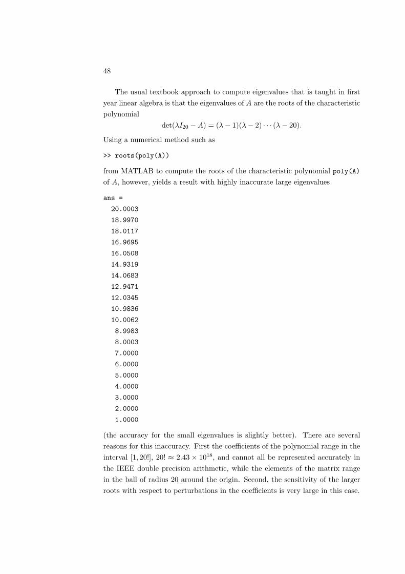
48

The usual textbook approach to compute eigenvalues that is taught in firstyear linear algebra is that the eigenvalues of A are the roots of the characteristicpolynomial

det(λI20 −A) = (λ− 1)(λ− 2) · · · (λ− 20).

Using a numerical method such as

>> roots(poly(A))

from MATLAB to compute the roots of the characteristic polynomial poly(A)of A, however, yields a result with highly inaccurate large eigenvalues

ans =

20.0003

18.9970

18.0117

16.9695

16.0508

14.9319

14.0683

12.9471

12.0345

10.9836

10.0062

8.9983

8.0003

7.0000

6.0000

5.0000

4.0000

3.0000

2.0000

1.0000

(the accuracy for the small eigenvalues is slightly better). There are severalreasons for this inaccuracy. First the coefficients of the polynomial range in theinterval [1, 20!], 20! ≈ 2.43 × 1018, and cannot all be represented accurately inthe IEEE double precision arithmetic, while the elements of the matrix rangein the ball of radius 20 around the origin. Second, the sensitivity of the largerroots with respect to perturbations in the coefficients is very large in this case.

49

In this section we have discussed the sensitivity (conditioning in particular)of a computational problem. This is a property of the problem and its mathematicalrepresentation in the context of the machine arithmetic used, and should not beconfused with the properties of the computational method that is implementedto solve the problem.

In practice, linear sensitivity estimates of the type

δy ≤ k(x)δx

are usually used neglecting second and higher terms in δx. This may sometimeslead to underestimation of the actual perturbation in the solution. Rigorousperturbation bounds can be derived by using the technique of non–linear perturbationanalysis [18, 16].

3.3 Computational algorithms

In this section we discuss properties of computational algorithms and in particulartheir numerical stability. To define formally what an algorithm is may not bean easy task. For our purposes, however, we shall need the following simplifiednotion of an algorithm.

An algorithm to compute y = f(x) is a decomposition

f = Fr Fr−1 · · · F1 (3.3)

of the function f which gives a sequence of intermediate results

xk = Fk(xk−1), k = 1, 2, . . . , r, (3.4)

with x0 = x and y = xr. Usually the computation of Fk(ξ) requires simplealgebraic operations on ξ such as arithmetic operations or taking roots, butit may also be a more complicated subproblem like solving a system of linearequations or computing the eigenvalues of a matrix.

The algorithm either gives the exact answer in exact arithmetic or for someproblems, like eigenvalue problems or the solution of differential equations, theanswer is an approximation to the exact answer in exact arithmetic. We will notanalyze the latter case here but we will investigate only what happens with thecomputed value y of xr when the computations are done in machine arithmetic.

It is important to mention that two different algorithms, say (3.3), (3.4) and

ξi = Φi(ξi−1), i = 1, 2, . . . , s, ξ0 = x,

50

wheref = Φs Φs−1 · · · Φ1,

for computing y = f(x) = ξs, may give completely different results in machinearithmetic although in exact arithmetic they are equivalent.

Example 3.4 Consider the computational problem

y = f(x) = x21 − x2

2

with a vector input x = (x1, x2) and a scalar output y. The problem may besolved by two algorithms f = F3 F2 F1 and f = Φ1 Φ2 Φ1, where

F1(x) = x21, F2(x) = x2

2, F3(x) = F1(x)− F2(x)

andΦ1(x) = x1 − x2, Φ2(x) = x1 + x2, Φ3(x) = Φ1(c)Φ2(x).

Which algorithm produces a more accurate result depends on the data x. Thedetailed behavior of these algorithms is considered in [27].

In what follows we suppose that the data x is in the normal range of themachine arithmetic with characteristics Xmax, Xmin, Emin and u, and that thecomputations do not lead to overflow or to a destructive underflow. As a resultthe answer computed by the algorithm (3.3) is y.

Our main goal will be to estimate the absolute error

E := ‖y − y‖

and the relative errore :=

‖y − y‖‖y‖ , y 6= 0,

of the computed solution y in case of a regular problem y = f(x) when the datax belongs to a given set X0 ⊂ X .

Definition 3.1 [23, 27, 11] The algorithm (3.3), (3.4) is said to be numericallystable on a given set X0 of data if the computed quantity y for y = f(x), x ∈ X0,is close to the solution f(x) of a problem with data x near to x in the sense that

‖y − f(x)‖ ≤ u a‖y‖, ‖x− x‖ ≤ u b‖x‖, (3.5)

where the constants a, b > 0 do not depend on x ∈ X0.

51

Definition 3.2 If the computed value y is equal to the rounded value round(y)of the exact answer y, then the result is obtained with the maximum achievableaccuracy.

To obtain the result with such an accuracy is the maximum that can be requiredform a numerical algorithm implemented in machine arithmetic.

For a problem for which the data is inexact, perhaps itself being subjectto rounding errors, numerical stability is in general the most we can ask of analgorithm. There are also other stability concepts for numerical algorithms.

Definition 3.3 If in Definition 3.1 we take a = 0, then the algorithm is callednumerically backward stable.

Thus backward numerical stability means that the computed result y is equalto the exact solution f(x) of a near problem (with data x close to x).

Definition 3.4 If in Definition 3.1 we take b = 0, then the algorithm is callednumerically forward stable.

Forward stability guarantees that the computed result y satisfies the inequality

‖y − y‖ ≤ u a‖y‖with a common constant a that does not depend on x ∈ X0. Thus the computedresult and the exact solution are u-close for all data x ∈ X0. However, manyclassical algorithms even for important problems in numerical linear algebra arenot forwardly stable as shown in the next example.

Example 3.5 For the solution of linear algebraic equations

Ay = c

with data x = (A, c) we cannot expect forward stability for all cases with A

invertible. Indeed, here the forward error ‖y−y‖ may be of order u k(A), where

k(A) = cond(A) := ‖A‖ ‖A−1‖is the condition number of A relative to inversion. But the number k(A) is notbounded when A varies over the set of all invertible matrices. If, however, A isrestricted to belong to the set of matrices with k(A) ≤ k0 for some moderateconstant k0 > 1, then the Gauss elimination algorithm and the algorithm basedon QR decomposition (both algorithms implemented with pivoting) will beforwardly numerically stable. Moreover, as shown by Wilkinson, these algorithmsare backwardly stable for all invertible matrices A.

52

The concept of backward stability, introduced by Wilkinson [28], tries torepresent the error of a computational algorithm by showing that the computedsolution is the exact solution of a problem with perturbed data, where theperturbation in the data is called the equivalent data error or the equivalentperturbation. For example, the elementary floating point operations are carriedout in a backward stable way, because (2.5) shows that the computed answer isthe correct one for slightly perturbed data x(1 + δ1) and y(1 + δ2), where δ1, δ2

are of order u.

It is clear from the definitions that backward stability implies stability, butthe converse is not true. In particular, some very simple algorithms are notbackwardly stable, see the next example.

Example 3.6 The computational problem

y = f(x) := 1 + 1/x,

is solved directly and very accurately for x ≥ 1. However, for x > 1/u we havey = 1 (a very accurate result!), but the method is not backwardly stable, sincef(x) > 1 for all x > 0.

3.4 A general accuracy estimate

In this section we shall derive a very elegant accuracy estimate for the solutioncomputed by a numerically stable algorithm. This estimate takes into accountall three major factors that govern the accuracy of the computational process.

Consider the solution of the computational problem y = f(x) by an algorithmthat is numerically stable on a set of data X0 (see Definition 3.1).

As in [23, 27], using the inequalities (3.5) and

‖f(x + h)− f(x)‖ ≤ K(x)‖h‖+ Ω(h)

(see (3.2)), we obtain the following estimate for the absolute error

‖y − y‖ = ‖y − f(x) + f(x)− f(x)‖≤ ‖y − f(x)‖+ ‖f(x)− f(x)‖≤ u a‖y‖+ K(x)‖x− x‖+ Ω(x− x)

≤ u a‖y‖+ u bK(x)‖x‖+ Ω(x− x).

53

Here K(x) is the absolute condition number (the Lipschitz constant) of theproblem y = f(x), while the constants a, b depend on the algorithm used andare given in Definition 3.1.

Dividing by ‖y‖ (in case y 6= 0) we find an estimate for the relative error

e :=‖y − y‖‖y‖ ≤ u

(a + bK(x)

‖x‖‖y‖ +

ω(x− x)u

). (3.6)

Since ω(x − x)/ε → 0 for ε → 0 we may ignore the third term in the bracketsin the right–hand side of (3.6) resulting in the approximate estimate

e ≤ u(

a + bK(x)‖x‖‖y‖

)= u(a + bk(x)) (3.7)

for the relative error in the computed solution.Note that for a backwardly stable algorithm we have a = 0 and hence

e ≤ u bk(x).

Similarly, for a forwardly stable algorithm we have b = 0 and

e ≤ u a

for some constant a which may be chosen independently on x ∈ X0 for a givenset X0 of data. In particular, we may assume that a is the supremum of e/uwhen x varies over X0.

It is instructive to point out that the famous rule of thumb is a particularcase of the estimate (3.7) when we presuppose a very stable algorithm witha = 0 and b = 1.

Having in mind the definition of the relative condition number k(x) of theproblem y = f(x) which is an “achievable” quantity, and the fact that the datax is usually rounded to x with ‖x − x‖ ≤ u, we may expect that for someproblems we shall have e ≥ u k(x). Hence for such problems we may assumethat

u k(x) ≤ e ≤ u(a + bk(x)).

Inequality (3.7) shows very clearly the influence of all the three major factorsthat determine the accuracy of the computed solution:

– the machine arithmetic (the rounding unit u and implicitly the range ofM through the requirement to avoid over– and underflows);

– the computational problem (the relative condition number k(x));

54

– the computational algorithm (the constants a and b).

Recalling that k(x) = K(x)‖x‖/‖y‖ we see that large relative errors in thecomputed solution may be expected when K(x) and/or ‖x‖ are large as well aswhen ‖y‖ is small. The latter is a well known rule in numerical analysis, namelythat large relative errors may occur when a small quantity is computed fromlarge initial or intermediate data. The catastrophic cancellation is a particularcase of this rule.

Inequality (3.7) is an example of a condition number based accuracy estimatefor the solution, computed in a machine arithmetic. In order to assess theaccuracy of results and to be able to trust numerical results, such condition andaccuracy estimates should accompany every computational procedure. Manymodern software packages provide such estimates [1, 3], see also

http://www.win.tue.nl/niconet

It is, however, unfortunate common practice in engineering simulation to turnthese facilities off, even though this service will warn the user of numericalmethods about possible failures.

We note that the stability of an algorithm does not itself guarantee automaticallya small error in the computed solution if the problem is ill conditioned, i.e. ifthe number uk(x) is about 1. The conclusion is that good results can only beexpected when a stable algorithm is used to solve a relatively well conditionedproblem.

3.5 Effects of modularization

In this section we illustrate some of the effects of modularization on the propertiesof computational processes.

As we have seen in (3.3), computational problems are typically modularized,which means that they are decomposed and solved by a sequence of subproblems.This facilitates the use of computational modules and is one of the reasons forsuccess of numerical analysis. But one should be aware that this modularizationmay lead to substantial numerical difficulties. This happens if one or more ofthe created subproblems Fk that are combined to get the decomposition is illconditioned. Consider for simplicity the decomposition

f = F2 F1

55

of a regular problem y = f(x) with absolute condition number K = K(x) whichis of order 1. Thus the original problem is very well conditioned.

First of all it may happen that one of the subproblems Fk is not regular.

Example 3.7 The scalar identity function y = f(x) := x may be decomposedas

f = F2 F1,

where F1(x) = x3 and F2(z) = z1/3. Here the function F2 is not Lipschitzcontinuous at the point z = 0. Hence one of the subproblems is not evenregular.

But even if the functions F1, F2 are Lipschitz continuous with constantsK1,K2 respectively, then it may happen that one (or both) of these constantsis large. We obtain the estimate

‖f(x + h)− f(x)‖ = ‖F2(F1(x + h))− F2(F1(x))‖≤ K2‖F1(x + h)− F1(x)‖ ≤ K2K1‖h‖,

where the quantity K2K1 may be much larger than the actual Lipschitz constantK of the function f at the point x.

Example 3.8 Consider the identity function y = f(x) := x in R2. Define

F1(x) = A−1x

andF2(z) = Az,

where the matrix A ∈ R2×2 is non–singular. The original problem is perfectlyconditioned with K = 1, while any of the constants K1 = ‖A−1‖ and K2 = ‖A‖may be arbitrarily large. Their product K1K2 = cond(A) may also be arbitrarilylarge.

If the computations are carried out with maximum achievable accuracy, thenthe computed value for A−1x is

F1(x) = (I2 + E1)A−1x,

whereE1 := diag(ε1, ε2)

and|ε1|, |ε2| ≤ u.

56

Similarly, the computed value for A(A−1x) becomes

(I2 + E2)AF1(x) = (I2 + E2)A(I2 + E1)A−1x,

whereE2 := diag(ε3, ε4)

and|ε3|, |ε4| ≤ u.

Suppose thatε1 = −ε2 = u ' 10−16, ε3 = ε4 = 0

and

A =

[a a + 1

a− 1 a

], x =

[1

−1

],

where a = 108. Then the computed result is

x = x + uξ,

whereξ = [ξ1, ξ2]>

and

ξ1 = 4a2 + 2a− 1,

ξ2 = 4a2 − 2a− 1.

Thus the actual relative error in the solution of the decomposed problem is

u‖ξ‖‖x‖ ' 4a2 u ' 4

and there are no correct digits in the computed result!

3.6 Solving some illustrative problems by MATLAB

The commands

>> x = [-1:-1:-18]’; x = 10.^x

will produce the 18–vector x = [10−1, 10−2, . . . , 10−18]>. With this vector wemay compute the quantities

y(k) =(1 + x(k))− 1

x(k), k = 1, 2, . . . , 18,

where x(k) are the elements of x, from

57

>> y = ((1 + x) - 1)./x

The result is

y =

1.00000000000000

1.00000000000000

0.99999999999989

0.99999999999989

1.00000000000655

0.99999999991773

1.00000000058387

0.00000000392253

1.00000008274037

1.00000008274037

1.00000008274037

1.00008890058234

0.99920072216264

0.99920072216264

1.11022302462516

0

0

0

Since the exact result is 1, we see that for k = 15 there is a relative error of 11percent while for k ≥ 16 the result is totally wrong with relative error of 100percent.

The computation of the vector of ones

y(k) =(1 + x(k))2 − 1− 2x(k)

x2(k)

by the command

>> y = ((1 + x).^2 - 1 - 2*x)./x.^2

will give

y =

1.00000000000002

1.00000000000006

58

0.99999999969742

0.99999999171889

1.00000139299870

0.99992436739695

1.01087806660425

-1.215...

...

We see that for k = 7 the result is computed by 11 percent relative error, whilefor k ≥ 8 the result is completely useless (for k = 8 even the sign is wrong andthe relative error is 221 percent).

Similarly, the computation of the quantities

y(k) =(1 + x(k))3 − 1− 3x(k)− 3x2(k)

x3(k),

all equal to 1, by the corresponding command gives

y =

1.00000000000035

0.99999999991242

0.99999950547556

0.99987350828302

1.10953927987086

-202.14...

...

The results are self-evident.The reader should be able to explain the above results and even give the

approximate value for k, where the computational catastrophe occurs.These results may be impressive for somebody who sees them for the first

time. Especially instructive is the fact that completely wrong results are displayedwith 15 (wrong) digits. Of course, neither MATLAB, nor the user’s computerare defective or guilty in any way. Simply this is the way the floating pointarithmetic works in certain cases.

Another easy computations contaminated with large errors are described inExercises 3.2 and 3.3.

3.7 Conclusions

The next issues are extracted from the first version of the paper [12].

59

In order to assess the accuracy of calculations and to be able to trustnumerical results, condition and accuracy estimates should accompany computationalprocedures and must be included in the corresponding computer codes. Usersmust be aware of possible difficulties accompanying the computational processand must know how to avoid them. These issues should also become an essentialpart of the curriculum to teach scientists and engineers how to use and developmodern computational software.

It is, however, unfortunately common practice in industrial use to turn thesefacilities off, even though this service will warn the user of numerical methodsabout possible failure. What is the reason for such irresponsible action? Onereason is that the computation of the estimates somewhat slows down themethod but, as we have learned in many discussions with engineers in industry,the main reason is that the user does not know how to interpret these warnings.But it should be clear that the developers of numerical software introducethese estimates not for the purpose of bothering the user with mathematicalover cautiones. The idea is to make the user aware of difficulties with thecomputational problem or the numerical method and it should be an essentialpart of the curriculum to teach scientists and engineers how to interpret anduse these warnings.


Exercise 3.1 The base e ' 2.7183 of the natural logarithms is equal to thelimes of the sequence (en), where

en :=(

1 +1n

)n

.

However, to compute approximately e as en for some large n is not simply a badidea but a catastrophe. For example taking n = 107 we compute e in MATLABwith a relative error of order 10−7 which is a good result. But taking n = 1016

we get the completely wrong result en = 1 with a relative error 0.63.Try to explain what happened (Hint: to compute e use the MATLAB

command exp(1)).

Exercise 3.2 Compute the expression

y =(((

2x

+ x

)− x

)− 1

x

)

60

for x = 10−k, k = 1, 2, . . . , 10. First compose the 10–vector X with componentsX(k) = 10−k and then use the command

>> Y = X.*(((2./X + X) - X) - 1./X)

to compute the 10-vector Y . Compare with the exact answer Y = [1, 1, . . . , 1]and comment the results.

Exercise 3.3 Form the 5× 5 matrix

>> A = gallery(5)

in MATLAB, and compute the vector v ∈ C5 of its eigenvalues by the command

>> v = eig(A)

The determinant of A, computed by det(A), is zero. Hence v should have a zeroelement. But the elements of v are of order 0.04 and are far from zero. Explainthe result (more details about matrix computations by MATLAB are given inpart II of the book).

61

PART II

NUMERICAL LINEAR

ALGEBRA

Chapter 4

Operations with matrices


In Part II of the book we consider the solution of the main problems of numericallinear algebra in machine arithmetic with rounding unit u.

In this chapter we shall consider the influence of rounding errors on theperformance of matrix operations in machine arithmetic. In this framework weconsider the data as exact, the only source of errors being the machine operationsthemselves.

We recall that matrices are denoted by upper case (usually Latin) letters.The element of the matrix A in position (p, q) is denoted as ap,q (or briefly apq),or A(p, q).

The vectors are denoted by lower (sometimes upper) case letters. The p–thelement of the vector x is denoted as xp or x(p).

We stress that the notations A(p,q) and x(p) are used in MATLAB, Scilaband SYSLAB to denote the corresponding elements of the matrix A and thevector x.

We note finally that the use of the indexes i or j in MATLAB may causeproblems since these letters are reserved for denoting the imaginary unit ı =√−1. So we advise the reader to use other letters for indexes.

4.2 Rounding of matrices

First we shall recall some special notations. If A is a matrix with elementsA(k, l) then |A| denotes the matrix absolute value (or the matrix module) of A

which is the matrix of the size of A and with elements |A(k, l)|.

63

64

If A and B are matrices of the same size then the component–wise inequality

A ¹ B

means that A(k, l) ≤ B(k, l) for all k, l. Similarly, A ≺ B means that A ¹ B

and A 6= B. We note that elsewhere A ≺ B is used do denote the relationsA(k, l) < B(k, l) for all k, l.

Definition 4.1 The matrix norm ‖ · ‖ is said to be monotone if ‖A‖ ≤ ‖B‖whenever |A| ¹ |B|.

We stress that the 1–norm

‖A‖1 = maxl

∑

k

|A(k, l)|,

the ∞–norm‖A‖infty = ‖A>‖1 = max

k

∑

l

|A(k, l)|

and the F–norm

‖A‖F =

∑

k,l

|A(k, l)|2

1/2

are monotone. The 2–norm, however, is not monotone as the next exampleshows.

Example 4.1 Consider the matrices

A =

[1 11 1

], B =

[1 1

−1.1 1

].

We have

|A| =[

1 11 1

]≺ |B| =

[1 1

1.1 1

]

but ‖A‖2 = 2 > ‖B‖2 = 1.5.

Let A be a real matrix with elements A(k, l) in the normal range of themachine arithmetic, i.e. either A(k, l) = 0 or

Emin ≤ |A(k, l)| ≤ Xmax.

Since in general the elements of A are not machine numbers then they cannotbe stored exactly in the computer memory. Thus in machine arithmetic instead

65

of A we shall have the rounded matrix A := round(A) with elements A(k, l)satisfying

A(k, l) = A(k, l)(1 + αk,l), (4.1)

where the quantities αk,l are relatively small, namely |αk,l| ≤ u. It follows from(4.1) that the component–wise inequality

|A−A| ¹ u|A| (4.2)

is fulfilled. Thus for all monotone norms we also have

‖A−A‖ ≤ u‖A‖. (4.3)

However, the estimate (4.2) is more informative than (refwhA1) because itsprovides a bound on the rounding error of each element of the matrix.

4.3 Summation of matrices

Definition 4.2 Let A and B be two matrices of the same size. Then their sumis the matrix C = A + B with elements C(k, l) = A(k, l) + B(k, l).

In the summation of these matrices in machine arithmetics instead of theexact sum C we obtain a matrix C = fl(A + B) which in general is differentfrom C. For the elements of C it is fulfilled that

C(k, l) = C(k, l)(1 + γkl), |γkl| ≤ u.

Hence|C(k, l)− C(k, l)| = |C(k, l)γkl| ≤ u|C(k, l)|

and|C − C| ¹ u|C|.

Hence for any monotone norm, and in particular for the 1-norm and the F-norm,we have

‖fl(A + B)− (A + B)‖ ≤ u‖A + B‖.Therefore, if A + B 6= 0, then

‖fl(A + B)− (A + B)‖‖A + B‖ ≤ u.

This estimate shows that the summation of two matrices in machine arithmeticis performed with small relative error of the order of the rounding unit u.

66

Of course, if for some k, l the elements A(k, l) and−B(k, l) are close approximatenumbers, then the relative error in the element C(k, l) = A(k, l) − (−B(k, l))may be large but this is not due to the execution of the machine operation A+B

itself.

4.4 Multiplication of matrices

In this section we shall analyze the computation of the product of two matrices inmachine arithmetic. There are several concepts for the product of matrices. Weshall consider the standard multiplication of matrices according to the followingdefinition.

Definition 4.3 Let A be a matrix of size m × n and B be a matrix of sizen×p. Then the product of A and B is the m×p matrix C = AB with elementsC(k, l) =

∑ns=1 A(k, s)B(s, l).

The standard product is associative in the sense that (AB)C = A(BC)and we write ABC for any of this quantities. This product also satisfies thedistributive rules (A1 + A2)B = A1B + A2B and A(B1 + B2) = AB1 + AB2. Inthe above relations it is supposed that the sizes of the involved matrices allowthe correct performance of the corresponding matrix operations.

Consider first two non–orthogonal vectors a, b ∈ Rn. It may be shown thatthe computation of the scalar product

(a, b) := a>b =n∑

k=1

akbk

is done with a relative error, for which we have the estimate

|fl(a>b)− a>b||a>b| ≤ u

n‖a‖ ‖b‖|a>b| .

On modern computer platforms, however, and for most modern systems fornumerical computations, the multiplier n in the above estimate can be replacedwith 1 or with a constant, close to 1. As Parlett says, this multiplier reflectsour abilities to estimate the error rather than the behavior of the actual error.

But nevertheless the relative error in the computation of the scalar productmay be very large if the scalar product a>b is small compared to ‖a‖ ‖b‖ (whenthe vectors a and b are almost orthogonal), i.e. if

‖a‖ ‖b‖|a>b| À 1. (4.4)

67

However, there are situations when the computation of the scalar product isdone with the maximum possible accuracy in the sense that

|fl(a>b)− a>b||a>b| ≤ u, (4.5)

see also Section 4.5.

Using the estimate (4.4) it can be shown that, given two matrices A ∈ Rm×n

and B ∈ Rn×p with AB 6= 0, their product is computed in machine arithmeticwith a relative error satisfying the estimate

‖fl(AB)−AB‖F

‖AB‖F≤ un

‖A‖F‖B‖F

‖AB‖F.

This relative error may be very large since the quantity

‖A‖F‖B‖F

‖AB‖F

is not bounded (the denominator ‖AB‖F can be arbitrarily small compared to‖A‖F‖B‖F).

Of course, if the computations are so organized that the scalar product iscomputed with maximum accuracy then the product of two matrices is alsocomputed with maximum accuracy, with a relative error of order u.

There is an important particular case when the machine product of twomatrices is always computed with small relative error. Let for example thematrix A = [a1, a2, . . . , an] has orthonormed columns ak ∈ Rm, i.e., ‖ak‖ = 1and a>k al = 0 for k 6= l (see also Chapter 5). Then we have

‖A‖F =√

n, ‖AB‖F = ‖B‖F

and hence‖fl(AB)−AB‖F

‖AB‖F≤ un3/2.

This is a very good result which shows that the multiplication with an orthogonalmatrix is not dangerous in machine arithmetic. This is reflected in the rulethat the numerically reliable matrix algorithms involve only orthogonal (unitaryin the complex case) transformations. A certain exception here is the Gausselimination algorithm with pivoting for the solution of linear algebraic equations.

68

4.5 Maximum accuracy computations

An important aspect in modern numerical computations, developed in the last30 years, is related to the computational algorithms which guarantee the maximumachievable accuracy in the particular machine arithmetic. If y = f(x) 6= 0 is thecomputational problem and y is the result, computed in machine arithmetic withrounding unit u, the answer is with maximum achievable accuracy if the relativeerror ‖y − y‖/‖y‖ is of order u. For example, such an algorithm guaranteesthat the computed scalar product fl(a>b) ∈ M of two vectors a, b ∈ Rn is theclosest to a>b ∈ R machine number. This result may not be improved since itcorresponds to the rounding error in writing the number a>b in the computermemory.

It may be observed that, up to now, algorithms with maximum accuracy areable to solve a number of relatively simple problems (such as the scalar productof two vectors or the product of two matrices) with errors, comparable with theerrors in rounding the scalar results to the nearest machine numbers. However,the development of such algorithms is a recent tendency in numerical analysis.

On the other hand, it is known that in modern personal computers theeffect of maximum accuracy is achieved in an almost automatic manner sincethe arithmetic operations in the processor are done with much higher precisionthan the corresponding overall machine precision suggests. More details aregiven in [27].

4.6 Matrix operations by MATLAB

We recall that the symbols i and j are reserved in MATLAB for the imaginaryunit ı =

√−1 and we shall avoid using them as indexes. Instead, we may use k

and l or p and q. We also note that MATLAB is case sensitive, i.e. the systemmakes a difference between the quantities denoted as A and a. In contrast,SYSLAB is case insensitive.

If we have an m× n matrix A, the command

>> size(A)

will return the pair m, n. Hence, if x is a row n–vector, we shall have size(x)

= 1, n. If x is a column n–vector, then the command size(x) will give thepair n, 1. For vectors we have also the command

>> length(x)

69

which gives n for both row and column n–vectors x.Note that the symbol >> is generated automatically at the beginning of

the command line in the command window of MATLAB1, and that in variousversions of MATLAB there may be different symbols for beginning of the commandrow.

Vectors and matrices may be defined in MATLAB in different ways.

Example 4.2 The commands

>> for p=1:5, x(p)=p^2; end

>> x

will produce and display the vector

x =

1 4 9 16 25

with elements xp = x(p) = p2, p = 1, 2, 3, 4, 5.Similarly, the commands

>> for k=1:10, for l=1:10, A(k,l)=1/(k+l-1);

end

end

will generate the 10×10 Hilbert matrix A with elements A(k, l) = 1/(k + l−1),k, l = 1, 2, . . . , 10.

The command

>> x = [a:h:b]

will produce a row vector x with first element x(1) = a, second element x(2) =a+h, etc. The last element of x, of the form a+nh, is the number with modulusnot exceeding |b| and closest to b. If a = b the result shall be x = a, If a < b

and h < 0 the result will be an empty matrix (of size 1 by 0). The same resultwill be obtained for h = 0.

Example 4.3 The command

>> x = [1:0.3:2]

1Further on this symbol may be omitted.

70

will produce the vector

x =

1.0000 1.3000 1.6000 1.9000

Also, we have

>> [2:-0.4:-1]

ans =

2.0000 1.6000 1.2000 0.8000 0.4000 0.0000 -0.4000 -0.8000

The integer n–vector x with elements 1, 2, . . . , n may also be produced bythe simple command

>> x = 1:n

Another way to define vectors and matrices is to input the elements of thecorresponding array one by one.

Example 4.4 The commands

>> A = [1 -3 0; pi 4 sqrt(2)]

will give the 2× 3 matrix A,

A =

1.0000 -3.0000 0

3.1416 4.0000 1.4142

Note that we put a space between the elements of A, and semicolon ; for thebeginning of the next row of A. The same effect is achieved by using commasfor distinguishing between elements as in the command

>> A = [1,-3,0;pi,4,sqrt(2)]

After the commands

>> format long

>> A

the matrix A will be displayed within 15 decimal digits.

Arrays can be read also from outer files, and matrices may be constructedalso by blocks.

71

Example 4.5 Suppose that we already have four matrices A11, A12, A21 andA22 of sizes m×n, m×p, q×n and q×p, respectively . Then the (m+q)×(n+p)–matrix

A :=

[A11 A12

A21 A22

]

may be constructed as

>> A = [A11, A12; A21, A22]

Once a matrix A or a vector x are defined, the commands

>> A(k,l)

>> x(p)

will produce the element of A in position (k, l) and the element of x in positionp, respectively.

The commands

>> A(:,q)

>> A(p,:)

will give the q–th column and p–th row of A, respectively.Similarly, the command

>> A(p:k,q:l)

returns the submatrix of A with elements at the crossing of rows p, p + 1, . . . , k

and columns q, q + 1, . . . , l, of A.If the m× n matrix A is real, the command

>> A’

will produce the transposed n×m matrix A> with elements A>(k, l) = A(l, k).But if the matrix A is complex, the same command will give the complexconjugate (or Hermite conjugate) n×m matrix AH = A

> with elements AH(k, l) =A(l, k).

Example 4.6 If x and y are column vectors, the command

>> z = [x’,y’]’

will return the vector z =

[x

y

]with length(z) = length(x) + length(y).

72

In order to find the transpose A> of a complex matrix A one may use thecommand

>> A.’

If A is a matrix with elements A(k, l), the commands

>> triu(A)

>> tril(A)

will produce the upper triangular part and lower triangular parts of A, respectively.In particular, triu(A) is a matrix of the size of A and elements A(k, l) if k ≤ l

and zero otherwise.The command

>> diag(x)

where x = [x1, x2, . . . , xn] is a vector, produces the diagonal n × n matrixdiag(x1, x2, . . . , xn) with the elements of x on its main diagonal. If A is anm× n matrix, then

>> diag(A)

gives the k–vector of the diagonal elements of A, where k := minm,n.

Example 4.7 For a square matrix A the command

>> triu(A) + tril(A) - diag(diag(A))

will return the matrix A (prove!).

The summation of two matrices, or arrays A and B of the same size isperformed in MATLAB simply as

>> A + B

The standard multiplication of the matrices A and B is done by the command

>> A*B

Of course, here the number of columns of the matrix A must be equal to thenumber of rows of the matrix B.

If A and B are arrays of the same size, we may define their H’Adamardproduct C = A B from

73

>> C = A.*B

We recall that C = A B is a matrix of the size of A and B with elementsC(k, l) = A(k, l)B(k, l), i.e. the H’Adamard multiplication is done element–wise.

The dot notation above is typical for array operations. However, for summationand subtraction the dot notation is not necessary since the operation ± is doneautomatically in MATLAB. If e.g. B is of the size of A and has no zero elements,we may define the array

>> C = A./B

with elements C(k, l) = A(k, l)/B(k, l).In the above considerations the matrix sizes must agree in order to guarantee

the correct performance of the corresponding matrix operations. If this isnot the case MATLAB will return an error message of the type Error using

(here follows the description of the operation such as +, −, ∗, etc.) Matrix

dimensions must agree.We stress that in MATLAB the term dimension is sometimes used instead

of size for matrices and vectors. Mathematically this may be arguable since thedimension is an attribute of a subspace rather than of a vector or a matrix.

In MATLAB there are some “strange” matrix operations. If A is a matrixwith elements A(k, l) and a is a scalar, then the operation

>> B = A + a

produces a matrix B of the size of A and with elements B(k, l) = A(k, l) + a.Also, if a is a scalar, and A has only nonzero elements, then the command

>> B = a./A

gives a matrix B of the size of A with elements B(k, l) = a/A(k, l).If A is a square matrix and m ∈ N, we may define the matrix power Am

inductively by Am := AAm−1, where A0 is the identity matrix. In MATLABAm may be computed simply from

>> A^m

Note, however, that for an arbitrary matrix A (which may not even be square),the command

>> A.^m

74

will produce the matrix of the size of A and with elements (A(k, l))m.The scalar product (or dot product)

xHy =n∑

k=1

xkyk

of the vectors x, y ∈ Cn is computed by the command

>> dot(x,y)

Note that in the complex case the order of the vectors x, y in dot(x,y) isimportant. And some authors define the dot product of x and y as yHx, whichis the complex conjugate to xHy.

There is a command in MATLAB for computation of the Kronecker (ortensor) product C = A⊗B of the matrices A and B of arbitrary sizes, namely

>> C = kron(A,B)

We recall that if A is m× n and B is k × l then

A⊗B ∈ Cmk×nl

is an m × n block matrix with blocks of size k × l, where the block in position(p, q) is A(p, q)B.

For 3–vectors x and y with elements xk and yk, we may find the so calledvector, or cross product x× y by the command

>> z = cross(x,y)

We recall that

z = [x2y3 − x3y2, x3y1 − x1y3, x1y2 − x2y1]>.

There are special commands for generating some special arrays. Let m andn be positive integers. The command

>> eye(n)

produces the identity n× n matrix In = diag(1, 1, . . . , 1). The command

>> eye(m,n)

creates an m × n matrix with ones on the main diagonal and zeros otherwise,e.g.

75

>> eye(2,3)

ans =

1 0 0

0 1 0

Obviously, eye(n,n) is the same as eye(n).

The commands

>> zeros(m,n)

>> ones(m,n)

form m× n matrices of zeros and ones, respectively. When m = n one may usethe short commands zeros(n) and ones(n).

Example 4.8 If the matrix A is m× n, then the commands

>> eye(size(A))

>> zeros(size(A))

>> ones(size(A))

will return a diagonal m × n matrix with ones on the diagonal, an m × n zeromatrix and an m× n matrix of ones, respectively.

Some other specific matrices are generated as follows.

The command

>> compan(p)

where p = [p1, p2, . . . , pn+1] is a real or complex (n + 1)-vector, creates thecompanion matrix of the polynomial

P (x) = p1xn + p2x

n−1 + · · ·+ pnx + pn+1.

We stress that in MATLAB an n–th degree polynomial P is identified with the(n+1)–vector p of its coefficients with p(1) 6= 0. A vector [0, 0, . . . , 0, a, b, . . . , c]with several zero elements in first positions and a 6= 0, defines the same polynomialas the vector [a, b, . . . , c].

The command

>> hadamard(n)

76

generates a Hadamard n× n matrix H. The elements of H are −1 or 1 and H

satisfies H>H = nIn. It is supposed that n, n/12 or n/20 is a power of 2.Hankel and Toeplitz matrices, having many applications, are defined and

constructed in MATLAB as follows.An n × n Hankel matrix Hn is symmetric and constant across its anti–

diagonals. The Hankel matrix Hn is determined by its first column c and itslast row r (with c(n) = r(1)). Hence there is a (2n− 1)–vector h, such that theelements of Hn are determined by Hn(k, l) = h(k + l − 1) for k, l = 1, 2, . . . , n.

Example 4.9 The Hankel 4× 4 matrices have the form

H4 =

h1 h2 h3 h4

h2 h3 h4 h5

h3 h4 h5 h6

h4 h5 h6 h7

The command

>> H = hankel(c)

creates a Hankel matrix whose first column is c and whose elements belowits main anti–diagonal are zero. In Example 4.9 this will be the case withh5 = h6 = h7 = 0.

The command

>> H = hankel(c,r)

creates a Hankel matrix with first column c and with last row r (note that thelast element of c and the first element of r must be equal).

An n × n Toeplitz matrix Tn is, in general, non–symmetric and constantacross its diagonals. The Toeplitz matrix Tn is determined by its first column c

and its first row r (with c(1) = r(1)).Hence there is a (2n−1)–vector t, such that the elements of Tn are determined

by Tn(k, l) = t(k − l + 1) for k ≥ l and Tn(k, l) = t(n + l − k) for k < l andk, l = 1, 2, . . . , n.

Example 4.10 The Toeplitz 4× 4 matrices have the form

T4 =

t1 t5 t6 t7

t2 t1 t5 t6

t3 t2 t1 t5

t4 t3 t2 t1

77

The command

>> T = toeplitz(c,r)

returns a Toeplitz matrix with first column c and with first row r (note that thefirst element of c and the first element of r must be equal).

The command

>> T = toeplitz(r)

returns a real symmetric Toeplitz matrix with first row r when r is real. When r

is a complex vector, the matrix toeplitz(r) will also be complex and Hermitian.The command

>> hilb(n)

produces the Hilbert n×n matrix with elements 1/(k + l− 1) in position (k, l).The inverse Hilbert n× n matrix is created by the command

>> invhilb(n)

The reader is advised to create Hilbert and inverse Hilbert matrices in therational format format rat.

The command

>> pascal(n)

produces the Pascal n×n integer matrix with elements from the Pascal triangle.The command

>> V = vander(c)

where c is a column n–vector, creates the n×n Wandermonde matrix Vn whose(n − 1)–th column is c (the elements of the n–th column of Vn are all equal to1). Thus the elements of V are V (k, l) = (c(l))n−k for k, l = 1, 2, . . . , n.

The Wilkinson eigenvalue test matrix is produced by the command wilkinson.The command

>> magic(n)

generates a magic (n × n)–square. This is an integer matrix with pairwisedisjoint elements from 1 to n2 with row, column and diagonal sums all equal ton(n2 + 1)/2. Note that n must not be 2.

78

Example 4.11 The command magic(2) will produce the matrix

[1 34 2

]with

column sums, equal to 5. But this is not a magic square since row sums are4 and 6, while diagonal sums are 3 and 7 (as we mentioned above, the magicsquare cannot be 2× 2).

For n = 3 and n = 4 we shall obtain the magic squares

>> magic(3)

ans =

8 1 6

3 5 7

4 9 2

and

>> magic(4)

ans =

16 2 3 13

5 11 10 8

9 7 6 12

4 14 15 1

For numerical experiments and other purposes it is useful to have densematrices of arbitrary dimensions. The command

>> A = rand(m,n)

will produce an m × n matrix A with elements A(k, l) randomly distributedbetween 0 and 1. The short command

>> A = rand(n)

will create a random n × n matrix A. Now the reader can easily constructmatrices with random elements between any two numbers a and b.

Random matrices with normally distributed elements may be generated bythe functions

>> A = randn(m,n)

>> A = randn(n)

79

which are similar to the functions rand(m,n) and rand(n), respectively.MATLAB contains a gallery of interesting matrix examples developed by N.

Higham. The reader may find a description of the gallery by the help commandhelp gallery.

The maximum and minimum elements of the real vector x may be found bythe commands

>> max(x)

>> min(x)

respectively.The command

>> y = abs(x)

returns the vector y = |x| whose elements y(p) are the absolute values |x(p)| ofthe elements of x (here x may be a complex vector).

Let A be an m × n matrix, and let k and l be two positive integers withkl = mn. Then the command

>> reshape(A,k,l)

will return the k× l matrix whose elements are taken column–wise from matrixA. If kl 6= mn the program will give an error message. Hence the column–wisevector representation a := vec(A) of A, which is an mn–vector, may be formedby the command

>> reshape(A,m*n,1)

or, automatically, by the somehow cumbersome function

>> reshape(A,(size(A))(1)*(size(A))(2),1)

The command

>> linspace(a,b)

produces a row 100–vector of linearly equally spaced points between the numbersa and b. The command

>> linspace(a,b,n)

creates a similar row n–vector.The command

80

>> logspace(a,b)

produces a row 50–vector of logarithmically spaced points between 10a and 10b.The command

>> logspace(a,b,n)

returns a similar row n–vector.


Exercise 4.1 Create Hilbert and inverse Hilbert matrices Hn and H−1n for n =

5, . . . , 15. Check whether the product of the computed quantities Hn and H−1n

is the identity matrix In.

Exercise 4.2 Generate Pascal matrices Pn of orders n = 3, 4, . . . , 10. Computetheir determinants det(Pn) by the command det and their inverses P−1

n by thecommand inv.

Exercise 4.3 Write a program which generates k random m×n matrices whoseelements are: (i) uniformly, and (ii) normally distributed random variables inthe interval [a, b] (here the integers k,m, n and the reals a, b must be input data).

Exercise 4.4 Generate a sequence of n–vectors c for a fixed n ≥ 2 with pairwise disjoint elements. Find the determinants det(vander(n)) of the correspondingVandermonde matrices Vn formed by vander(c) and whose (n−1)–th column isc. Formulate and prove a hypothesis about det(Vn) as a function of the elementsof the vector c.

Chapter 5

Orthogonal and unitary

matrices


In this chapter we recall the basic facts about real orthogonal and complexunitary matrices. These matrices play a fundamental role in the computationalalgorithms of modern numerical linear algebra.

5.2 Main definitions and results

In this section we give the definitions and main properties of orthogonal andunitary matrices.

Definition 5.1 A real n × n matrix U = [u1, u2, . . . , un] ∈ Rn×n, uk ∈ Rn, iscalled orthogonal if

U>U = In.

We note that this term is not very appropriate since orthogonality is a relationbetween two objects.

It follows from the above definition that UU> = In (prove this!).The columns up of an orthogonal matrix are orthonormed (orthogonal and

normed) in the sense that u>p uq = 0 for p 6= q and u>p up = ‖up‖2 = 1.According to Definition 5.1 an orthogonal matrix U is non–singular and its

inverse is

U−1 = U>.

81

82

Thus the inversion of an orthogonal matrix requires no arithmetic operations andis done exactly in machine arithmetic. This is very important from numericalpoint of view.

The multiplication of a real vector x by an orthogonal matrix U rotatesthe vector without changing its 2–norm. Indeed, setting y = Ux we see thaty>y = x>U>Ux = x>x and hence ‖y‖2 = ‖x‖2.

Also, it follows from the definition of orthogonality that the elements U(k, l)of U satisfy

−1 ≤ U(k, l) ≤ 1,

and that

‖U‖2 = 1, ‖U‖F =√

n . (5.1)

The matrix A ∈ Rm×n has orthonormed columns if A>A = In. In this caseby necessity rank(A) = n ≤ m.

Similarly, the matrix A ∈ Rm×n has orthonormed rows if the matrix A> ∈Rn×m has orthonormed columns, i.e. if AA> = Im. Here rank(A) = m ≤ n.

For real orthogonal matrices it follows from In = U>U that det(In) =det(U>U) and hence

1 = det(U>) det(U) = (det(U))2.

Therefore det(U) = 1 or det(U) = −1.

Definition 5.2 Orthogonal matrices with determinant 1 are called (pure) rotations,while these with determinant −1 are called reflections.

In the complex case we may define both orthogonal matrices and unitarymatrices.

The n × n complex orthogonal matrices (again a name that is not veryappropriate) are defined as in the real case by U>U = In. Note that for acomplex nonzero vector u ∈ Cn we may have u>u = 0, e.g. u = [1, ı]>, whereı =

√−1. However, in the complex case unitary matrices are usually moreinteresting from practical point of view than orthogonal matrices.

Definition 5.3 The matrix U ∈ Cn×n is called unitary if

UHU = In.

83

We recall that UH = U>, i.e. UH(p, q) = U(q, p).

The columns up of an unitary matrix U satisfy uHp uq = 0 for p 6= q and

uHp up = ‖up‖2 = 1.

It follows from Definition 5.3 that an unitary matrix U ∈ Cn×n is nonsingularwith

U−1 = UH

and its spectral and Frobenius norms satisfy (5.1). Also we have |U(k, l)| ≤ 1.Similarly to the real case, the multiplication of a (complex) vector by an

unitary matrix preserves the 2–norm of the vector. A generalization of thisproperty is given below.

If the matrix U is unitary we have | det(U)|2 = 1 and hence the quantitydet(U) lies on the unit circle in the complex plane C.

Real orthogonal (or complex unitary) matrices can be used in order totransform real (or complex) vectors and matrices into simpler condensed formwhich contains zeros in prescribed positions.

These matrices are very favorable for numerical computations. Let U, V beunitary matrices and A be an arbitrary matrix of appropriate size. Then

‖UAV ‖2 = ‖A‖2,

‖UAV ‖F = ‖A‖F.

Hence unitary transformations of the form A 7→ UAV preserve the 2–norm andthe Frobenius norm of the matrix A.

Let the complex n × n matrix U = U0 + ıU1 be unitary, where U0, U1 arereal n× n matrices and ı =

√−1 is the imaginary unit. Since UH = U>0 − ıU>

1 ,it follows from the unitarity of U that

U>0 U0 + U>

1 U1 = In,

U>0 U1 = U>

1 U0.

Similarly, if the complex matrix U is orthogonal, we have

U>0 U0 − U>

1 U1 = In,

U>0 U1 + U>

1 U0 = 0.

Real orthogonal and complex unitary matrices U are particular cases of theso called normal matrices A which are characterized by the property A>A =AA> in the real case and AHA = AAH in the complex case. Hence, given such

84

a matrix U , there is a unitary matrix V such that the matrix Λ := V HUV isdiagonal with the eigenvalues λk of U on its diagonal. Since Λ is also orthogonal,we have |λk| = 1. Hence the eigenvalues of U lie on the unit circle in the complexplane C. This is a more general property than the fact that det(U), being theproduct of the eigenvalues, lies on the unit circle.

Important classes of real orthogonal (or complex unitary) matrices are theelementary reflections and the elementary rotations. Elementary (or Householder)reflections are considered further on.

5.3 Orthogonal and unitary matrices in MATLAB

Let A ∈ Rm×n be a matrix with rank(A) = r. Then an important task is toconstruct an orthonormed basis u1, u2, . . . , ur ⊂ Rm for the range

Rg(A) := Ax : x ∈ Rn ⊂ Rm

of this matrix.The function

>> U = orth(A)

produces the matrix

U = [u1, u2, . . . , ur] ∈ Rm×r

with columns up ∈ Rm such that u>p uq = δpq, where δpq is the Kronecker deltaequal to 0 when p 6= q and to 1 when p = q.


>> A = [1 1 2;2 2 4;3 3 -1]

A =

1 1 2

2 2 4

3 3 -1

creates the matrix A ∈ R3×3 with rank(A) = 2 since columns 1 and 2 of A

coincide and columns 1 and 3 are linearly independent. This may be checkedby the command

>> rank(A)

85

Now the command orth(A) will produce the orthonormed 3× 2 matrix

ans =

-0.3904 -0.2182

-0.7807 -0.4364

-0.4880 0.8729

with range, equal to Rg(A).

To produce (generically) an orthogonal n × n matrix U one may use thecommands

>> A = rand(n); U = orth(A);

(the use of semicolons will prevent the display of the corresponding matrices).This approach works if the randomly generated matrix A is nonsingular whichwill almost surely be the case.

Another way to create a real orthogonal n×n matrix Q is to use the commandsequence

>> A = rand(n); [Q,R] = qr(A)

Note that the second command above finds the QR decomposition A = QR ofthe real randomly generated n× n matrix A.

A complex unitary matrix Q may be found from

>> A = rand(n) + i*rand(n); [Q,R] = qr(A)

Note that the last two commands rand(n) produce two different random n× n

matrices.Orthogonal and unitary matrices are widely used in MATLAB, Scilab and

SYSLAB in order to ensure the reliability and accuracy of the correspondingcomputational algorithms.


Exercise 5.1 Show that any orthogonal matrix U ∈ R2×2 has one of the twoforms

R :=

[cosϕ − sinϕ

sinϕ cosϕ

], S :=

[cosϕ sinϕ

sinϕ − cosϕ

]

for some ϕ ∈ [0, 2π). Find the determinants of R and S.

86

Exercise 5.2 Describe the set of all 2× 2 complex unitary matrices.

Exercise 5.3 Show that the set of n × n complex orthogonal matrices is notbounded for n > 1.

Exercise 5.4 Let U = U0 + ıU1 be a complex n×n matrix, where the matrices

U0, U1 are real. Show that the real (2n×2n)–matrix

[U0 −U1

U1 U0

]is orthogonal

if and only if the matrix U is unitary.

Chapter 6

Orthogonal and unitary

matrix decompositions


In this chapter we consider two very useful orthogonal (unitary in the complexcase) decompositions of a general matrix: the QR decomposition, or brieflyQRD, and the singular value decomposition, or briefly SVD. Another importantorthogonal decomposition of a square matrix – the Schur decomposition, isstudied in Chapter 9.

6.2 Elementary unitary matrices

A general unitary matrix may be decomposed into a product of “elementary”unitary matrices. There are several types of matrices, considered as elementary.Among them are the plane (or Givens) rotations and the elementary (or Householder)reflections.

Definition 6.1 An elementary complex plane rotation (or Givens rotation) is aunitary matrix, which differs from the identity matrix in at most four positions,occupied by the elements of a 2× 2 unitary matrix and has determinant 1.

More precisely, a rotation in the (p, q)-plane, p < q, is an n × n matrix Rpq,whose (k, l) elements rkl are determined as follows. The 2× 2 matrix

[rpp rpq

rqp rqq

](6.1)

87

88

is unitary and rkl is the Kronecker delta if k, l ∩ p, q = ∅.An elementary real plane rotation is defined similarly. It is a real orthogonal

matrix with the structure of Rpq, where the matrix (6.1) is orthogonal.Another type of elementary unitary matrices are the elementary reflections.

Let u ∈ Cn be a non-zero vector.

Definition 6.2 The matrix

H(u) := In − 2uuH

uHu∈ Cn×n

is said to be an elementary complex (or Householder) reflection.

It follows from this definition that

H(u) = H(αu)

for each nonzero scalar α. The matrix H = H(u) is both Hermitian and unitary,

HH = H, HHH = In.

Elementary real reflections are defined similarly as

H(v) := In − 2vv>

v>v∈ Rn×n, 0 6= v ∈ Rn.

The matrix H = H(v) is both symmetric and orthogonal,

H> = H, H>H = In.

The multiplication of a vector x ∈ Cn by a reflection H(u) is reduced to thecalculation of a single scalar product uHx, multiplication of a vector by a scalarand substraction of two vectors according to

H(u)x = x−(

2uHx

uHu

)u.

In particular we have

H(u)u = u−(

2uHu

uHu

)u = u− 2u = −u

and det(H(u)) = −1.Elementary reflections take their name from the fact that the mapping x 7→

H(u)x is a reflection relative to the one–dimensional subspace (hyperplane)

Ker(uH) = x ∈ Cn : uHx = 0.

89

Indeed, we have

uH(x + H(u)x) = 2uH

(x− uuHx

uHu

)= 2(uHx− uHx) = 0.

Thus the vector u is orthogonal to the sum of x and its image H(u)x. Equivalently,u is collinear to the difference x−H(u)x since x and H(u)x are of equal 2–norm.Thus, a multiplication with H(u) reflects any vector relative to Ker(uH).

Based on the above discussion we have an elegant solution to the followingproblem. Given two different vectors x, y ∈ Cn of equal 2–norm, find a unitarymatrix U , which transforms x into y, i.e. y = Ux. It follows from the reflectionproperty of H(u) that a solution of this problem is U = H(x− y) since

H(x− y)x = y, ‖x‖2 = ‖y‖2 > 0.

It is often necessary to transform a non–zero vector x into a form with onlyone nonzero element in the k–th position. Suppose that the vector x ∈ Cn

is not proportional to the k–th column ek of the identity matrix In (if it is,there is nothing to transform). Let α ∈ C and |α| = 1. Then the requiredtransformation is

H(x− y)x = y, y := α‖x‖2ek 6= x. (6.2)

In the real case we have α = ±1 and

H(x− y)x = y, y := ±‖x‖2ek. (6.3)

The choice of α in (6.2), respectively of the sign in (6.3), is done fromnumerical considerations in order to avoid possible cancellations in subtractingclose quantities. If the argument of xk is ϕk, i.e. xk = ρk exp(ıϕk), then wechoose the argument of α as ϕk + π which gives α = − exp(ıϕk). In this waythe k–th element of the vector x− y becomes (ρk + ‖x‖2) exp(ıϕk).

If in the real case if xk is non–negative (respectively negative) we choosey = ‖x‖2ek (respectively y = −‖x‖2ek).

Since the matrix H(x∓ ‖x‖2ek) is both Hermitian and unitary we have

x = H(x− y)y = α‖x‖2H(x− y)ek = α‖x‖2hk,

where hk is the k–th column of H(x − y). Hence, a matrix H(u) transforms avector x 6= 0 into α‖x‖2ek if and only if its k–th column hk is collinear to x.

Now we may solve the following problem. Given an unit vector x ∈ Cn findan n × (n − 1) matrix V such that the matrix U := [x, V ] is unitary. If x is

90

collinear to some column ek of In, then V contains the other columns of In.Suppose now that x is not collinear to a column of In. Let h1, h2, . . . , hn be thecolumns of the reflection H(x∓ e1) which transforms x into e1. Then a solutionof our problem is

V = [h2, h3, . . . , hn].

Indeed, in this case x = ±h1.Using a sequence of reflections an m × n matrix A of rank r ≥ 1 may be

reduced to a condensed upper triangular form R = QHA, where Q is a productof reflections (see the next section). Let m1 < m2 < · · · < mr be the numbers ofthe first linearly independent columns of A. Then the matrix R with elementsrkl may be characterized as follows.

– The last m− r rows (if any) of the matrix R are zero.– the first non–zero element in the k–th row (k ≤ r) of R is rk,mk

> 0.

6.3 QR decomposition

Let A ∈ Cm×n be an arbitrary matrix of rank r := rank(A) ≥ 1 (the caseA = 0 is not interesting). Then, as shown above, there exist an unitary matrixU ∈ Cm×m and an upper triangular matrix R ∈ Cm×n such that

A = QR (6.4)

Definition 6.3 The representation (6.4) is known as QR decomposition1, orunitary-triangular decomposition of the matrix A.

Partitioning the matrices Q and R as

Q = [Q1, Q2], Q1 ∈ Cm×r, R =

[R1

0

], R1 ∈ Cr×m

we may write the decomposition in the form

A = Q1R1. (6.5)

The relation (6.5) is the so called economic QR decomposition.The QR decomposition is a very useful tool in numerical linear algebra. In

particular it is used for solution of linear algebraic equations and least squaresproblems as well as for rank determination.

1Sometimes the QR decomposition is called QR factorization.

91

From computational point of view it is convenient to rearrange the columnsof A so as the diagonal elements R1(k, k) of the matrix R1 to satisfy theinequalities

|R1(1, 1)| ≥ |R1(2, 2)| ≥ · · · ≥ |R1(r, r)| > 0. (6.6)

For this purpose a permutation matrix E ∈ Rn×n is constructed so that thedecomposition

AE = QR

to satisfy (6.6).

The QR decomposition of A is constructed in r − 1 steps. Suppose fordefiniteness that r = n ≤ m.

At the first step we construct a Householder reflection Q1 := H1 ∈ Cm×m

such that H1a1 = [×1, 0, . . . , 0]>, where a1 ∈ Cm is the first column of A and×1 is the only nonzero element of the transformed vector H1a1.

At the second step we set Q2 := diag(1,H2), where H2 is an (m−1)×(m−1)reflection such that H2a2 = [×2, 0, . . . , 0]>. Here a2 is the vector with elementsA2(2, 2), A2(3, 2), . . . , A2(m, 2), where A2 := Q1A1.

We may continue this process until we obtain the matrix Ar−1 = R.

6.4 Singular value decomposition

For any matrix A ∈ Cm×n of rank r := rank(A) ≥ 1 there exist two unitarymatrices U ∈ Cm×m, V ∈ Cn×n and a diagonal matrix S ∈ Cm×n such that

A = USV H. (6.7)

Here

S :=

[Σ 00 0

], Σ := diag(σ1, σ2, . . . , σr) ∈ Rr×r.

Definition 6.4 The numbers

σ1 ≥ σ2 ≥ · · · ≥ σr > 0

are said to be the positive singular values of the matrix A. The columns v1, v2, . . . , vn ∈Cn of V are called the (right) singular vectors of A. The representation (6.7) isknown as the singular value decomposition, or briefly SVD, of the matrix A.

92

It may be shown that the positive singular values of A are the positive squareroots of the positive eigenvalues of the Hermitian matrix AHA (or AAH).

The singular value decomposition may also be written as

A =r∑

k=1

σkukvHk ,

where u1, u2, . . . , um ∈ Cm are the columns of the matrix U . We see that herethe matrix A of rank r is represented as the sum of r rank–one matrices σkukv

Hk .

When the matrix A is real, the matrices U and V may also be chosen realand in this case they are orthogonal matrices.

The SVD is one of the most useful tools in numerical linear algebra. Inparticular, the SVD is applicable to the rank determination of a matrix and tothe solution of linear algebraic equations and least squares problems.

Another useful decomposition involves a pair of matrices with equal numberof columns. Let A ∈ Cm×p and B ∈ Cn×p. Then there exist unitary matricesU ∈ Cm×m, V ∈ Cn×n (UHU = Im, V HV = In), a matrix W ∈ Cp×q withq := minm + n, p and non–negative diagonal matrices C ∈ Cm×q, D ∈ Cn×q,such that

A = UCWH, B = V SWH, (6.8)

whereC>C + S>S = Iq. (6.9)

Definition 6.5 The relations (6.8), (6.9) define the generalized singular valuedecomposition, or briefly GSVD, of the matrix pair (A,B).

6.5 Orthogonal and unitary decompositions by MATLAB

We recall that the orthogonal–triangular decomposition, known as QR decomposition,of the matrix A ∈ Cm×n, is a factorization of A of the form

A = QR,

where the matrix Q ∈ Cm×m is unitary, i.e. QHQ = Im, and the matrix R ∈Cm×n is upper triangular. When the matrix A is real, the matrix Q is realorthogonal (Q>Q = Im).

The command

>> qr(A)

93

returns only the matrix R. The command

>> [Q,R] = qr(A)

computes the matrices Q and R, while the command

>> [Q,R,E] = qr(A)

produces a permutation matrix E ∈ Rn×n and the matrices Q and R such thatAE = QR. In this case the absolute values |R(k, k)| of the diagonal elementsR(k, k) of R are not increasing with k.

When m > n the function

>> [Q1,R1] = qr(A,0)

computes the “economy” QR decomposition in which Q1 ∈ Cm×n is a matrixwith orthonormed columns.

The singular value decomposition

A = USV H

of the real or complex (non–zero) m× n matrix A is found by the command

>> [U,S,V] = svd(A)

Here the matrices U ∈ Cm×m and V ∈ Cn×n are unitary in the complex case,and real orthogonal in the real case. The matrix S is diagonal of size m × n

with the singular values σ1, σ2, . . . , σp of A on its main diagonal in descendingorder, where p = minm,n. When r := rank(A) < p we shall have σr > 0 andσr+1 = σr+2 = · · · = σp = 0.

When A is the zero matrix the command [U,S,V] = svd(A) will returnU = Im, S = 0 and V = In.

The short command

>> s = svd(A)

returns the p–vector s, containing the singular values of A in descending order.If m > n we may compute the “economy size” singular value decomposition

>> [U1,S1,V] = svd(A,0)

where U1 contains the first n columns of U , and S1 contains the first n rows ofS.

The generalized singular value decomposition of a pair of matrices A ∈ Cm×p,B ∈ Cn×p (with the same number of columns) may be found by the command

94

>> [U,V,W,C,S] = gsvd(A,B)

Here the matrices U ∈ Cm×m and V ∈ Cn×n are unitary, W is a p × q matrixwith q = minm + n, p, and C ∈ Cm×q, S ∈ Cn×q are nonnegative diagonalmatrices, such that

A = UCWH, B = V SWH, CHC + SHS = Iq.

The short command

>> s = gsvd(A,B)

returns the q–vector s of generalized singular values. In fact, we have

s = sqrt(diag(C’*C./diag(S’*S))

More details about the MATLAB functions svd and gsvd may be found, asusual, by the commands help gsvd and help svd.


Exercise 6.1 Generate a sequence of random small size matrices A and B withthe same number of columns and find:

– the QR decompositions of A and B;– the singular value decompositions of A and B;– the generalized singular value decompositions of the pairs (A,B).

Exercise 6.2 Prove that the positive singular values of the nonzero matrix A

are the positive square roots of the positive eigenvalues of the matrix AHA (orAAH).

Exercise 6.3 Generate a sequence of random square matrices by the commandAn = rand(n) for n = 10, 50, 100, 500. Most probably these matrices willbe non–singular. Find the SVD [Un,Sn,Vn] = svd(An) of each matrix An.When An is non–singular then we should have A−1

n = VnS−1n U>

n . Compute thequantities dn = norm(Bn - Cn), where Bn = inv(An) and Cn = Vn*inv(Sn)*Un’.Theoretically dn must be zero. Investigate the behavior of dn with the increaseof n.

Chapter 7

Linear algebraic equations

7.1 Statement of the problem

In this chapter we shall use the Euclidean norm for vectors and, according tothis, the spectral norm of matrices, i.e. we assume ‖ · ‖ = ‖ · ‖2. We recall that

‖x‖2 :=

(n∑

i=1

|xi|2)1/2

for a real or complex vector x = [x1, x2, . . . , xn]>, and

‖A‖2 :=√

λmax(AHA)

for a matrix A, where AH := A> and λmax(M) is the maximum eigenvalue of

the non–negative definite matrix M .Consider the solution of the real linear vector equation

Ax = b (7.1)

in machine arithmetic with rounding unit u. We suppose that A ∈ Rn×n is anon–singular (invertible) matrix, b ∈ Rn is a given non–zero vector (otherwisethe solution is trivially zero) and x ∈ Rn is the solution. The case when A, b

and x may be complex quantities is studied in the same way.The more general matrix equation

AX = B, (7.2)

where A ∈ Rn×n, B = [B1, B2, . . . , Bm] ∈ Rn×m, Bk ∈ Rn, and X = [X1, X2, . . . , Xm] ∈Rn×m, Xk ∈ Rn, is reduced to m copies

AXk = Bk, k = 1, 2, . . . , m,

95

96

of equation (7.1).Sometimes the row–wise versions of the equations (7.1) and (7.2) is used,

namelyyA = c (7.3)

andY A = C, (7.4)

where A is an n× n invertible matrix as above, c and y are row n–vectors andY, C are m × n matrices. If Yk and Ck are the rows of Y and C, respectively,then equation (7.4) is reduced to m equations YkA = Ck, k = 1, 2, . . . ,m, oftype (7.3).

Obviously, equations (7.3) and (7.4) may be written in the form (7.1) and(7.2), respectively, e.g. A>y> = c> and A>Y > = C>.

The more general matrix linear equation

r∑

k=1

MkXNk = B, (7.5)

whereMk ∈ Rm×m, Nk ∈ Rn×n, B ∈ Rm×n

are given matrices and X ∈ Rm×n is the solution, can be reduced formally toequation (7.1). Indeed, setting

A :=r∑

k=1

N>k ⊗Mk ∈ Rmn×mn, b := vec(B) ∈ Rmn

and x := vec(X) ∈ Rmn, we obtain an equation of type (7.1). Here M⊗N is theKronecker product of the matrices M and N , while vec(B) is the column–wisevector representation of the matrix B.

Of course, the possibility to reduce equation (7.5) into the form (7.1) doesnot mean that this is the numerically correct way to solve this equation. Usuallymatrix equations of type (7.5) are solved directly, by special methods, andwithout reduction into vector form.

7.2 Formal solutions

Formally, the solution of equation (7.1) may be written as

x = A−1b,

97

where A−1 ∈ Rn×n is the inverse of the matrix A ∈ Rn×n. Similarly, the solutionof equation (7.3) is

y = cA−1.

However, these representations of the solutions are rarely used in practice becausethe calculation of A−1 and the computation of the products A−1b and cA−1 maynot be accurate and/or efficient.

Moreover, the computation of the matrix F := A−1 (if necessary for somepurpose) is done by solving n algebraic equations

Afk = ek, k = 1, 2, . . . , n,

for the columns fk ∈ Cn of the matrix F = [f1, f2, . . . , fn], where ek is the k–thcolumn of the identity matrix In.

There is also another elegant formal (but practically useless) way to representthe elements x1, x2, . . . , xn of the solution vector. Indeed, we have

b = Ax =n∑

l=1

xlal, (7.6)

where al are the columns of the matrix A = [a1, a2, . . . , an]. For a given integerk ∈ 1, n consider the matrix

Ak = Ak(b) := [a1, . . . , ak−1, b, ak+1, . . . , an],

obtained by replacing the k–th column ak of A by the vector b. In view of (7.6)we have

det(Ak) = det

[a1, . . . , ak−1,

n∑

l=1

xlal, ak+1, . . . , an

]

=n∑

l=1

xl det[a1, . . . , ak−1, al, ak+1, . . . , an]

= xk det(A).

Since det(A) 6= 0 we get

xk =det(Ak)det(A)

, k = 1, 2, . . . , n. (7.7)

These are the Cramer formulae – a beautiful and useless (for n > 3) representationof the elements of the solution vector x = [x1, x2, . . . , xn]>.

Unfortunately, some people still think that this is the proper way to solvelinear equations.

98

7.3 Sensitivity of the solution

Consider the sensitivity of the problem of solving equation (7.1). Let δA, δb beperturbations in the data A, b, such that

‖δA‖ <1

‖A−1‖ .

This inequality guarantees that the perturbed matrix A + δA is also invertible.Let x + δx be the (unique) solution of the perturbed equation

(A + δA)(x + δx) = b + δb. (7.8)

It follows from (7.8) that

δx = A−1(δb− δAx)−A−1δAδx

and

‖δx‖ ≤ ‖A−1‖(‖δb‖+ ‖δA‖ ‖x‖) + ‖A−1‖‖δA‖ ‖δx‖.

Since ‖A−1‖ ‖δA‖ < 1 we have

‖δx‖ ≤ ‖A−1‖(‖δb‖+ ‖δA‖ ‖x‖)1− ‖A−1‖ ‖δA‖ .

The sensitivity estimate becomes particularly elegant when relative norm–wise perturbations are used,

δx :=‖δx‖‖x‖ , δA :=

‖δA‖‖A‖ , δb :=

‖δb‖‖b‖ .

We get

δx ≤ kA(ηδb + δA)1− kAδA

, (7.9)

where

kA = cond(A) := ‖A‖ ‖A−1‖ =σmax(A)σmin(A)

is the condition number of A relative to inversion in the spectral norm, and

η = η(A, b) :=‖b‖

‖A‖ ‖x‖ =‖b‖

‖A‖ ‖A−1b‖ .

It follows from Ax = b that

‖b‖ ≤ ‖A‖ ‖x‖

99

and hence η ≤ 1. Thus we come to the simpler widely used but less accurateestimate

δx ≤ kA(δb + δA)1− kAδA

. (7.10)

On the other hand we have

‖A−1b‖ ≤ ‖A−1‖ ‖b‖

which yields1

‖A−1b‖ ≥1

‖A−1‖ ‖b‖and η ≥ 1/kA. Therefore the following estimates for η are valid

1kA

≤ η ≤ 1.

The lower bound 1/kA for η is achieved when b is a multiple of the right singularvector of the matrix A−1, corresponding to its maximum singular value equal to‖A−1‖. In this case it may not be a good idea to replace η with 1. Moreover, theestimate (7.9) with η < 1 can be arbitrarily many times better than the estimate(7.10), in which we have replaced η with 1. Unfortunately the improved estimate(7.9) is not very popular among common users.

Consider now the case when the perturbations are due to rounding errorswhen writing the data in computer memory. Then we may assume that

δA, δb ≤ u

and hence

δx ≤ kA(1 + η)u1− kAu

.

When kAu ¿ 1 we get the approximate inequality

δx ≤ kA(1 + η)u.

Thus the quantity

cA := kA(1 + η) ≤ 2kA

can be regarded as an estimate of the relative condition number of the solutionto the algebraic linear vector equation (7.1).

100

7.4 Computational methods

The most used methods for the numerical solution of equation (7.1) (in themedium size case when n is of order 1000) are the Gauss elimination method1

and the method of QR decomposition. The Gauss elimination method is basedon the so called LU decomposition of the matrix A, considered below.

In the Gauss method the non–singular matrix A or, more generally, thematrix EA, where E is a permutation matrix, is decomposed as

A = LU,

orEA = LU,

where L is a lower triangular matrix with elements, equal to 1, on its maindiagonal and U is an upper triangular matrix with non–zero diagonal elements.The permutation matrix E is found from the condition to have a maximumabsolute value pivot element at each step of the reduction of A into uppertriangular form. The last two decompositions are known as lower–upper decompositions,or briefly, LU decompositions of A.

The decomposition EA = LU corresponds to the so called eliminationwith partial pivoting. The pivoting is very important in order to improve thenumerical behavior of the Gauss elimination method.

Setting y = Ux we may write the equation Ax = b as

Ly = c, c := Eb.

Since the matrix L = [lpq] is lower triangular with lpp = 1, we have

y1 = c1, (7.11)

lp1y1 + lp2y2 + · · ·+ lp,p−1yp−1 + yp = cp, p = 2, 3, . . . , n,

where yp and cp are the elements of the vectors y and c, respectively. Now theelements of the vector y are determined recursively from (7.11) starting with y1.

Having the vector y, the solution x is found from the linear triangular system

Ux = y

starting from the last equation (see the QR decomposition method describedbelow).

1This method had been used in China some 3,000 years ago for n = 3.

101

In the QR decomposition method the matrix A (or EA) is decomposed as

A = QR,

where the matrix Q is orthogonal and the matrix R = [rpq] is upper triangularwith nonzero diagonal elements. Thus x is obtained from the triangular system

Rx = c, c := Q>b.

First we solve the last scalar equation rnnxn = cn, obtaining xn = cn/rnn. Thenwe solve the (n− 1)–th equation

rn−1,n−1xn−1 + rn−1,nxn = cn−1,

obtainingxn−1 =

cn−1 − rn−1,nxn

rn−1,n−1.

At the (n + 1− k)–th step we obtain

xk =1

rkk

ck −

n∑

p=k+1

rkpxp

,

where the quantities xn, xn−1, . . . , xk+1 are already computed. This processcontinues until we compute x1 at the n–th step.

Another method to solve the linear equation

Ax = b,

applicable to singular and rectangular matrices A, is the reduction of A into theso called row echelon form.

Let A be an m× n (non–zero) matrix. Then there is a permutation matrixE ∈ Rm×m, a lower triangular matrix L ∈ Cm×m with unit diagonal, and anm× n matrix R in row echelon form so that

EA = LR.

Here the matrix R of rank

r = rank(R) = rank(A) ≤ minm,n

satisfies the following conditions.1. The first r rows of R are linearly independent, while the rest m− r rows

(if any) are zero.

102

2. The first non–zero element of any non–zero row (called pivot element) isequal to 1. The rest of the elements of the column containing a pivot are allzeros.

3. The pivot of every row with number p ∈ 2, r is placed to the right of thepivot of row p− 1.

Example 7.1 The 4× 5 matrix

R =

0 1 0 • 00 0 1 • 00 0 0 0 10 0 0 0 0

of rank 3 is in row echelon form (we denote unspecified elements by •).

Note that if the matrix A ∈ Cn×n is non–singular, its row echelon form issimply the identity matrix In.

Some authors define the row echelon form R in a less condensed manner:the pivot elements in R are nonzero (positive in particular) and the elements inthe column above the pilot may not be zero.

Example 7.2 The less condensed echelon form R for the matrix of Example 7.1is

R =

0 + • • •0 0 + • •0 0 0 0 +0 0 0 0 0

,

where unspecified elements are denoted by • and positive elements are markedby +.

The low echelon form makes it possible to analyze the equation

Ax = b, A ∈ Cm×n, b ∈ Cm, (7.12)

where the nonzero matrix A may be singular (if m = n), or rectangular (m 6= n)of any rank r = rank(A) between 1 and minm,n.

Theoretically, the system (7.12) has a solution if and only if the geometriccondition

b ∈ Rg(A) (7.13)

103

is fulfilled, where

Rg(A) := Ax : x ∈ Cn ⊂ Cm

is the range (or image) of the matrix A. The equivalent algebraic necessary andsufficient condition for existence of a solution is

rank[A, b] = rank(A). (7.14)

Note that rank(A) ≤ rank[A, b] ≤ 1 + rank(A). Hence the equation (7.12) hasno solution if and only if rank[A, b] = 1 + rank(A).

Checking either the geometric condition (7.13) or the algebraic rank condition(7.14) for existence of a solution is not a good computational practice. The goodprocedure here is simply to transform the augmented matrix [A, b] into somecondensed form which clearly indicates whether or not the system is solvable.

Let x0 ∈ Cn be a fixed (or particular) solution of (7.12).

Definition 7.1 The general solution (or the set of all solutions) of equation(7.12)

X := x ∈ Cn : Ax = b

is the linear variety

X = x0 + Ker(A).

Here

Ker(A) := x ∈ Cn : Ax = 0 ⊂ Cn

is the kernel (or null–space) of the matrix A.Note that if the equation has no solution then X = ∅ so the set X is always

correctly defined.It follows from Definition 7.1 that the solution depends on n−r free parameters

– this number is the dimension of the subspace Ker(A)). In particular, whenthe solution exists it is unique if and only if when r = n, or equivalently whenKer(A) is the zero subspace.

To analyze equation (7.12) let us form the augmented matrix

C := [A, b] ∈ Cm×(n+1)

and compute its row echelon form D. We have the following possibilities.– If D has zero rows (and hence r < m) then there are m − r redundant

equations which may be deleted obtaining an equivalent equation with r rows.

104

– If D has a row of the type [0, 0, . . . , 0, 1] (it will be the row r + 1) then theequation has no solutions.

– If A is square and nonsingular, then (at least theoretically) the matrix D

shall have the form D = [In, x], where x is the solution. In this case the solutionmay formally be written as x = A−1b.

Note, however, that the computation of the row echelon form D of the matrixC matrix may be a difficult numerical problem similar to the computation ofthe inverse of a matrix. The less condensed form D of C may sometimes becomputed more reliably.

Consider finally the case when the matrix A is real symmetric, or complexHermitian, and positive definite (and hence nonsingular). Then it may bedecomposed uniquely as

A = LLH,

or asA = UHU,

where the matrix L is lower triangular (or R is upper triangular) with positivediagonal elements. This special case of LU decomposition is called the Choleskydecomposition. It requires about half of the arithmetic operations necessary forthe standard LU decomposition and is thus more efficient and (eventually) moreaccurate.

7.5 Errors in the computed solution

For both methods, described in the previous section, we have the followingestimate for the relative error in the solution x ∈ Rn, computed in machinearithmetic:

δ =‖x− x‖‖x‖ ≤ uψ(n)cond(A), cond(A) := ‖A‖ ‖A−1‖,

where ψ(n) is a polynomial in n of degree not greater than 3. This estimateis usually pessimistic which means that in practice it is much larger than theactual relative error δ in the computed solution x.

According to the famous heuristic “rule of thumb”, if

u cond(A) < 1

then there are (probably)

[− log10(u cond(A))]

105

true decimal digits in the computed solution, where [z] is the entire part of thenumber z > 0.

7.6 Solving linear algebraic equations by MATLAB

Linear algebraic equationsAx = b,

where the matrix A ∈ Cn×n is non–singular, b ∈ Cn is a given vector and x ∈ Cn

is the solution vector, are solved by the command

>> x = A\b

The same command is used when b and x are matrices of the same size.If the matrix A is singular or ill–conditioned, there will be a warning message,

e.g. Matrix is close to singular or badly scaled. Results may be inaccurate.

In this case the condition number cond(A) of the matrix A will be estimatedas 1016 or more. Accordingly, the reciprocal value rcond(A) of cond(A) will beestimated as 10−16 or less. We recall that 10−16 is written as e-016 in MATLAB.

A warning message will also be issued if the sizes of A and b are incompatible.Hence the computational algorithm which MATLAB uses for solving linear

algebraic equations is reliable.A reliable algorithm may not solve any problem. But it warns the user when

the solution is eventually contaminated with large errors.The LU decomposition of the matrix A is found by the command lu. In

particular, the function

>> [L,U] = lu(A)

computes an upper triangular matrix U and a (not necessarily lower triangular)matrix L which is a product of lower triangular and permutation matrices suchthat A = LU .

The command

>> [L,U,E] = lu(A)

gives the lower triangular matrix L, the upper triangular matrix U and thepermutation matrix E in the LU decomposition EA = LU of the matrix A.

The row echelon form of a general matrix A is computed in MATLAB bythe command

106

>> R = rref(A)

The same is done by the function

>> R = rref(A,tol)

using a tolerance tol to decide whether an element is considered as negligible.The Cholesky decomposition of a positive definite matrix A is computed by

the command

>> R = chol(A)

which gives the upper triangular matrix R such that A = RHR.

7.7 Norms and condition numbers in MATLAB

Vector norms are computed in MATLAB as follows. The Euclidean, or 2-norm

‖x‖2 :=

(n∑

k=1

|xk|2)1/2

of the n–vector x with elements xk is computed by the function

>> norm(x)

The command

>> norm(x,inf)

is the same as

>> max(abs(x))

and computes the norm

‖x‖∞ := max|xk| : k = 1, 2, . . . , n.

The 1–norm

‖x‖1 :=n∑

k=1

|xk|

is found by the command

>> norm(x,1)

107

More generally, for p ≥ 1 the so called Holder p–norm

‖x‖p :=

(n∑

k=1

|xk|p)1/p

may found by the function

>> norm(x,p)

The 2–norm

‖A‖2 := max‖Ax‖2 : x ∈ Cn, ‖x‖2 = 1

of the m×n matrix A, equal to its maximum singular value σ1, or to the squareroot of the maximum eigenvalue of the matrix AHA, is found by the command

>> norm(A)

The 1–norm

‖A‖1 := max‖Ax‖1 : x ∈ Cn, ‖x‖1 = 1

of the m×n matrix A, equal to the maximum of the 1–norms of its columns, iscomputed from

>> norm(A,1)

The function

>> norm(A,inf)

computes the norm

‖A‖∞ := max‖Ax‖∞ : x ∈ Cn, ‖x‖∞ = 1,

of A, which is equal to the maximum of the 1–norms of its rows. Obviously,

‖A‖∞ = ‖A>‖1.

Finally, the Frobenius norm

‖A‖F :=

m,n∑

k,l=1

|akl|2

1/2

=√

tr(AHA)

of the matrix A with elements akl may be found by the command

108

>> norm(A,’fro’)

Note that

‖A‖F =

(r∑

k=1

σ2k

)1/2

,

where σ1 ≥ σ2 ≥ · · · ≥ σr > 0 are the positive singular values, and r is the rankof A.

The condition number

cond(A) = cond2(A) := ‖A‖2‖A−1‖2

of the nonsingular matrix A in the 2–norm is computed by the command

>> cond(A)

The function

>> rcond(A)

gives an estimate for the reciprocal 1/cond1(A) of the condition number

cond1(A) := ‖A‖1‖A−1‖1

of A in the 1–norm. If A is well conditioned then rcond(A) is close to 1. If A isvery ill conditioned, rcond(A) is about the size of the rounding unit u or evenless.


Exercise 7.1 Find in a closed form the condition numbers of the invertiblematrix

A =

[a b

c d

]∈ K2×2

in both the spectral and Frobenius norms, where K = R or K = C.

Exercise 7.2 If A and B are invertible matrices of the same size, prove that

B−1 −A−1 = B−1(A−B)A−1.

109

Exercise 7.3 Let A be an invertible matrix and δA be a perturbation in A

such that‖A‖ ‖δA‖ < 1.

Show that the following estimates

‖(A + δA)−1 −A−1‖‖A−1‖ ≤ kAδA

1− kAδA=

‖A−1‖ ‖δA‖1− ‖A−1‖ ‖δA‖ ,

‖(A + δA)−1 −A−1‖‖(A + δA)−1‖ ≤ kAδA = ‖A−1‖ ‖δA‖, kA := ‖A‖ ‖A−1‖,

are valid. Hint: for the first estimate use the technique from Section 7.3assuming that x and b are matrices, and b = In. Prove the second estimateusing the identity from Exercise 7.2.

Exercise 7.4 Let |A| = [|akl|] be the matrix module of the matrix A, i.e. thematrix of the modules of the elements of A. Consider the equation Ax = b

together with its perturbed version

(A + δA)(x + δx) = b + δb,

where A is an invertible n×n matrix. Prove that if the eigenvalues of the matrix

|A−1| |δA|

have modules less than 1, it is fulfilled that

|δx| ¹ (In − |A−1| |δA|) |A−1|(|δb|+ |δA| |x|).

This estimate is component–wise and may be much more informative than thenorm–wise estimates considered above.

Exercise 7.5 Let x be an approximate solution to the equation

Ax = b

with a square matrix A. Find the minimum norm perturbations δA, δb for whichthe vector x is an exact solution to the perturbed equation with data A + δA

and b + δb, i.e(A + δA)x = b + δb.

For this purpose find the so called backward error

min‖[δA, δb]‖F : (A + δA)x = b + δb

110

solving the linear least squares problem (see Chapter 8)

δAx− δb = b−Ax

with respect to the unknowns δA, δb.

Exercise 7.6 Show that for an invertible n×n matrix B and a nonzero n–vectory the relations

σmin(B)‖y‖ ≤ ‖By‖ ≤ σmax(B)‖y‖and

1‖B‖ ‖y‖ ≤

1‖By‖ ≤

‖B−1‖‖y‖

are valid. We recall that in the 2–norm it is fulfilled

σmin(B) =1

‖B−1‖ , σmax(B) = ‖B‖.

Exercise 7.7 Consider the linear algebraic equation Ax = b with a squareinvertible matrix A under perturbations δA, δb, such that the matrix A + δA isinvertible and ‖δb‖ < ‖b‖. Prove that the vector b + δb and the solution

x + δx = (A + δA)−1(b + δb)

of the perturbed equation are nonzero. Then justify the estimate

‖δx‖‖x + δx‖ ≤

kA(δA + δb)1− δb

.

Can you obtain a better estimate?

Exercise 7.8 Generate random linear systems Ax = b with a reference solutionx = [1, 1, . . . , 1]> by the commands

>> A = rand(n); b = A*ones(n,1)

Compute the solution by any of the command lines

>> x1 = A\b

>> x2 = inv(A)*b

>> [Q,R] = qr(A); x3 = R\(Q’*b)

Analyze the relative errors

>> ek = norm(xk - x)/sqrt(n)

111

in the computed approximation to the exact solution x, and compare them withthe heuristic bound eps*cond(A).

Make the same experiment with the matrix A = gallery(3), namely

A =

−149 −50 −154

537 180 546−27 −9 −25

.

Exercise 7.9 Determinants must be avoided in solving (even low size) linearalgebraic equations since the computation of determinants may not be accurateand/or efficient.

For n = 1, 2, . . . , 10 form the 3× 3 matrices

>> an = [0,zeros(1,2);zeros(2,1),tn];

>> bn = [tn,zeros(2,1);zeros(1,2),0];

where

>> tn = [10^n,10^n+1;10^n-1,10^n].

Since det(tn) = 1 we should have det(an) = det(bn) = 1, and det(cn) = 1,where cn=an*bn. Compute now the determinants of the matrices an, bn and cn

in MATLAB (or in SYSLAB, or in Scilab) by the function det and commentthe numerical disaster.

Exercise 7.10 Use the Cramer formulae (7.7) to derive explicit expressionsfor the elements of the matrix A−1 (such expressions are of theoretical interestmainly).

Chapter 8

Least squares problems


Consider the algebraic least squares problem

Ax ' b, (8.1)

whereA ∈ Rm×n, b ∈ Rm, x ∈ Rn, m À n,

which is formulated as an optimization problem for finding x so that

‖Ax− b‖ = min! (8.2)

Here usually ‖ · ‖ is the 2–norm although other norms are used as well.The solution x of the problem (8.2) satisfies the so called normal equation

A>Ax = A>b. When r = rank(A) = n the solution is unique and has the form

x = (A>A)−1A>b.

Note that this is a formal representation of the solution. In practice, thecomputation of the matrix A>A in machine arithmetic may lead to loss ofaccuracy.

Example 8.1 Let

A =

1 00 δ

0 0

, b =

110

,

where u < δ <√

u. Then the matrix A has condition number of order 1/δ andthe problem Ax = b has an unique solution x = [x1, x2]> = [1, 1/δ]>. In machine

113

114

arithmetic with rounding unit u the rank–two matrix A>A =

[1 00 δ2

]will be

rounded to the rank–one machine matrix fl(A>A) = diag(1, 0). As a result thenormal equation A>Ax = A>b becomes x1 = 1, 0 = δ and has no solution.

If r < n then the solution of the problem is not unique (the solution set isan n− r linear variety) and one may consider the additional condition

‖x‖ = min! (8.3)

Now the least squares problem (8.2), (8.3) has a unique solution. We shall referto (8.2), (8.3) as the standard least squares problem.

The least squares problem is formulated similarly in the complex case, aswell as in the general case when the number of equations m may be less, equalto, or larger than the number of unknowns n.

The name of the problem comes from the fact that in (8.2) we minimize infact the sum

‖r‖2 = r21 + r2

2 + · · ·+ r2m

of the squares of the components of the so called residual vector

r = r(x) := Ax− b.

There are various formulations of least squares problems. A problem arisingin optimization may be formulated by (8.2) under the additional requirementthat the elements xk of x are non–negative,

xk ≥ 0, k = 1, 2, . . . , n. (8.4)

Another least squares problem coming from statistics is to find an n–vectorx such that

Ax = b + ξ, (8.5)

where the m–vector ξ is normally distributed (m > n) with zero mean andcovariance matrix V ∈ Rm×m (V is symmetric positive definite). Here thesolution x minimizes the expression

(Ax− b)>V −1(Ax− b)

and formally is defined from

x = (A>V −1A)−1A>V −1b.

As in the standard least squares problem, this representation of the solution isusually not used for computations, see also the comments presented in the nextsection.

115

8.2 Computation of the solution

Theoretically the solution of (8.2), (8.3) may be computed from the conditionthat the vector r is orthogonal to the subspace Rg(A), spanned by the columnsof A. This gives

A>r = A>(Ax− b) = 0 (8.6)

or

A>Ax = A>b. (8.7)

Indeed, if r is orthogonal to any vector from Rg(A) it is also orthogonal tothe vector AA>r, i.e.

r>AA>r = ‖A>r‖2 = 0,

which gives A>r = 0.

An elegant but formal way to prove (8.6) or (8.7) directly (without considerationsabout orthogonality) is as follows. Since we want to prove that y := A>r = 0,suppose the opposite, i.e. that y 6= 0. Then z := Ay 6= 0 since

r>z = r>AA>r = y>y = ‖y‖2 > 0.

Setting

x := x− ‖y‖2

‖z‖2y

we get

‖Ax− b‖ =∥∥∥∥r − ‖y‖2

‖z‖2z

∥∥∥∥ = ‖r‖2 − 2r>z‖y‖2

‖z‖2+‖y‖4

‖z‖2

= ‖r‖2 − ‖y‖4

‖z‖2< ‖r‖2.

But this contradicts to the fact that x minimizes ‖r‖ = ‖Ax − b‖. HenceA>r = 0.

Equation (8.7) constitutes the so called normal form of the least squaresproblem. At first glance it seems preferable since it is (usually) an equationof much smaller size (m instead of n) with a symmetric non–negative definitematrix A>A. But in practice the formation of the matrix A>A should be avoidedsince it may lead to the loss of rank when the computations are done in machinearithmetic.

116

Example 8.2 Suppose that we use a machine arithmetic with rounding unit uand consider the matrix

A =

1 10 ε

0 0

,

where the quantity ε satisfies

u ≤ ε <√

u.

The matrix A is of full rank 2, which can well be recognized by the moderncomputer systems for matrix calculations.

If we form the matrix

A>A =

[1 11 1 + ε2

]

we see that it is again of rank 2, but after rounding the element in position (2,2)is written in the computer memory as 1. Hence the machine matrix

fl(A>A) =

[1 11 1

]

is of rank 1 and the rounded normal system may even have no solution! Thiswill be the case when e.g. b = [1, 1, 0]>.

Consider the solution of the problem with a matrix A of full column rank n

using the method of QR decomposition.Let

A = QR

be the QR decomposition of A, where the matrix Q ∈ Rm×m is orthogonal(Q>Q = Im) and the matrix R is of the form

R =

[R1

0

].

Here R1 ∈ Rn×n is an upper triangular non–singular matrix. If we set

Q>b =

[c

d

], c ∈ Rn,

then

‖Ax− b‖ = ‖QRx− b‖ = ‖Q(Rx−Q>b)‖ = ‖Rx−Q>b‖ = min!

117

Since

‖Rx−Q>b‖2 = ‖R1x− c‖2 + ‖d‖2

we must determine x = [x1, x2, . . . , xn]> as the solution to the equation

R1x = c = [c1, c2, . . . , cn]>.

Since the matrix R1 = [rkl] is upper triangular, this equation is solved directlyby back substitution, namely

xn =cn

rnn,

xn−1 =cn−1 − rn−1,nxn

rn−1,n−1,

· · · · · ·x1 =

c1 − r12x2 − r13x3 − · · · − r1nxn

r11.

In case when the matrix A is not of a full rank the least squares problem canbe solved by using the singular value decomposition of the matrix A as follows.

Let the rank of the matrix A ∈ Rm×n be r < minm,n. Then the singularvalue decomposition of the matrix A is

A = USV >,

where U ∈ Rm×m and V ∈ Rn×n are orthogonal matrices (U>U = Im, V >V =In) and

S :=

[Σ 00 0

]∈ Rm×n, Σ := diag(σ1, σ2, . . . , σr) ∈ Rr×r.

Here σ1 ≥ σ2 ≥ · · · ≥ σr > 0 are the singular values of A. We recall that theyare the square roots of the positive eigenvalues of the matrix A>A.

Setting y := V >x we obtain

r = Ax− b = USy − b = U(Sy − U>b).

Hence ‖r‖ = ‖Sy − U>b‖ and since ‖y‖ = ‖x‖ we have the new least squaresproblem

‖Sy − U>b‖ = min!

‖y‖ = min!

118

which is easily solvable since the matrix S is diagonal. Indeed, set

y :=

[u

v

], U>b :=

[c

d

],

where u, c ∈ Rr, v ∈ Rn−r, d ∈ Rm−r. Then

Sy − U>b =

[Σu

0

]−

[c

d

]=

[Σu− c

−d

].

Hence‖Sy − U>b‖2 = ‖Σu− c‖2 + ‖d‖2

and we see that the minimum of ‖Sy − U>b‖ is achieved when Σu = c, i.e.

u = Σ−1c.

Here the determination of u does not require an actual inversion of a matrix sinceΣ is a diagonal matrix, i.e. the elements uk of u are calculated very accuratelyfrom

uk =ck

σk, k = 1, 2, . . . , r.

In this case the minimum value of ‖Σy − U>b‖, equal to the minimum of valueof ‖Ax− b‖, is ‖d‖.

Up to now v is arbitrary. But

‖x‖2 = ‖y‖2 = ‖u‖2 + ‖v‖2 = ‖Σ−1c‖2 + ‖v‖2

and in order to minimize ‖x‖ = ‖y‖ one has to choose v = 0.Returning to the original unknown vector x we obtain the solution of the

least squares problem as

x = V

[Σ−1c

0

]= A†b.

Here A† ∈ Rn×m is the so called Moore–Penrose pseudoinverse of the matrix A,defined by the expression

A† := V S†U>,

where

S† :=

[Σ−1 00 0

]∈ Rn×m.

119

8.3 Error estimation

When using the computational scheme based on QR decomposition the errorestimate for the computed solution x is

δ :=‖x− x‖‖x‖ ≤ 6mnkAγ(A, b)u,

where

γ(A, b) := 1 + kAkA‖Ax− b‖+ ‖b‖

‖A‖ ‖x‖and

kA := cond(A) = ‖A‖ ‖A†‖

is the condition number of the full rank matrix A. Here A† ∈ Rn×m is thepseudoinverse of the matrix A. We recall that if

A = USV > ∈ Rm×n

is the singular value decomposition of the matrix A ∈ Rm×n of rank p, wherethe matrices U ∈ Rm×m and V ∈ Rn×n are orthogonal (U>U = Im, V >V = In)and

S = diag(σ1, σ2, . . . , σp, 0) ∈ Rm×n, σ1 ≥ σ2 ≥ · · · ≥ σp > 0,

then the pseudoinverse of A is

A† = V S†U> ∈ Rn×m, S† := diag(1/σ1, 1/σ2, . . . , 1/σp, 0) ∈ Rn×m.

8.4 Solving least squares problems by MATLAB

The algebraic linear least squares problem

Ax ' b,

where A ∈ Cm×n, b ∈ Cm is the data and x ∈ Cn is the solution, is computedby the command

>> x = A\b

This MATLAB command realizes the so called “left division” of the vector b

by the matrix A. We stress that the same command solves the linear algebraicequation Ax = b when A is a non–singular matrix.

120

Consider now the matrix least squares problem

AX ' B,

where B = [B1, B2, . . . , Bp] and X = [X1, X2, . . . , Xp] are m × p matrices withcolumns Bk and Xk, respectively. In this case the solution X, computed byleft division, will now minimize the norms ‖AXk − Bk‖ of the residual vectorsAXk −Bk.

The solution x of the least squares problem can also be expressed as

x = A†b,

where A† ∈ Cn×m is the pseudoinverse of A.The pseudoinverse Y := A† of A is produced by the command

>> Y = pinv(A)

The computation is based on the singular value decomposition of the matrix A.The computed pseudoinverse is in fact the pseudoinverse with a threshold

τ = maxm,n‖A‖u,

where u is the rounding unit of the machine arithmetic.The MATLAB command

>> Y = pinv(A,tol)

computes the pseudoinverse Y of A with a threshold tol, prescribed by the user.The least squares problem (8.2), (8.4) is solved by the command

>> x = nnls(A,b)

In turn, the solution of the problem (8.5) may be computed from

>> x = lscov(A,b,V)


Exercise 8.1 Show that the pseudoinverse A† ∈ Rn×m of A ∈ Rm×n is theunique matrix such that the solution x of the least squares problem

‖Ax− b‖ = min!

‖x‖ = min!

can be represented as x = A†b for all vectors b ∈ Rm (here ‖ · ‖ is the 2–norm).The same is valid when A, b and x are complex quantities.

121

Exercise 8.2 Form series of large size 2n× n random matrices A and random2n–vectors b. Find the solution to the corresponding least squares problemsAx ' b first by the command

>> x = A\b

and then by the function

>> xx = inv(A’*A)*(A’*b)

Compare the two solutions and the corresponding residual vectors (theoreticallythey are the same). Construct an example where the second approach leads tolarger errors.

Exercise 8.3 Generate series of random m × n matrices A and m–vectors b.Solve the corresponding standard least squares problems by the command

>> x = A\b

and the least squares problems with the constraints (8.4) by the command

>> xx = nnls(A,b)

Compare the solutions x and xx and the norms of the corresponding residualvectors.

Chapter 9

Eigenvalue problems

9.1 Main definitions and properties

In this section we give a survey of the main definitions and properties concerningthe so called eigenstructure (eigenvalues and eigenvectors) of real and complexsquare matrices.

Let A be an n× n matrix over R or C.

Definition 9.1 The number λ (real or complex) is said to be an eigenvalue ofA if there exists a nonzero n–vector u such that

Au = λu, (9.1)

or, equivalently,

(λIn −A)u = 0. (9.2)

The vector u is called an eigenvector, corresponding to the eigenvalue λ, and(λ, u) is called an eigenpair of the matrix A.

We stress that even if the matrix A is real, some (or all) of its eigenpairsmay be complex. Indeed, let λ = α + ıβ be a complex eigenvalue of A, whereα, β are real with β 6= 0, and u be the corresponding eigenvector. Then

Au = λu

and hence λ = α−ıβ is also an eigenvalue and u is an eigenvector, correspondingto λ.

123

124

Further on, we may look for the eigenvector u in the form u = r + ıs, wherethe vectors r, s are real. Substituting these expressions for λ and u in (9.1) weobtain

Ar = αr − βs,

As = βr + αs,

or

AU = UΛ,

where

U := [r, s] ∈ Rn×2, Λ :=

[α −β

β α

]∈ R2×2.

The column vector u above is also referred to as the right eigenvector of A

corresponding to the eigenvalue λ of A. We may also define the left eigenvectorw of A corresponding to the same eigenvalue λ. This is a row non–zero vectorsatisfying

wA = λw.

Hence AHwH = λwH. The column vector v := wH is also called a left eigenvectorof A. It follows from

vHA = λvH

that v is a (right) eigenvector of the matrix AH corresponding to the eigenvalueλ. When the matrix A is real, v is the (right) eigenvector of the matrix A>

Since equation (9.2) has a nonzero solution u, the matrix λIn − A must besingular. Indeed, in the opposite case the zero solution of (9.2) should be uniqueand there should not be a non–zero solution. Hence

hA(λ) := det(λIn −A) = 0, (9.3)

where In is the n× n identity matrix.

Definition 9.2 The algebraic equation (9.3) of degree n is called the characteristicequation of the matrix A and hA(λ) is called the characteristic polynomial ofA.

Clearly, the eigenvalues of the matrix A are the roots of its characteristicequation and vice versa. Usually we are interested in the collection λ1, λ2, . . . , λnof all n eigenvalues of the n× n matrix A counted according to their algebraic

125

multiplicity (as roots of the characteristic equation). The set of pair–wisedifferent eigenvalues of A is sometimes called the spectrum of A while thecollection of all eigenvalues is referred to as the full spectrum of A.

Thus the eigenvalues of a given matrix A are uniquely determined. Incontrast, the eigenvector u, corresponding to the eigenvalue λ of A, is notunique. In particular, the vector ku, where k is a nonzero scalar, will alsobe an eigenvector of A, associated with the same eigenvalue λ. Further on weshall usually suppose that the right and left eigenvectors are normed (in the2–norm) in the sense that

‖u‖ = ‖v‖ = 1.

The characteristic equation of A has the form

λn − c1λn−1 + · · ·+ (−1)ncn = 0.

Here the coefficient ck = ck(A) of the characteristic polynomial hA(λ) of A isthe sum of principal minors of A of order k. For example,

c1 = tr(A), cn = det(A).

In practice, the coefficients ck are not computed as sums of the principalminors of A. If, for some reasons, the coefficients ck are to be computed, thisis done by specialized algorithms. As a rule, the computation of ck from theelements of A should be avoided.

According to the famous Caley–Hamilton theorem, any matrix satisfies itscharacteristic equation in the sense that

hA(A) = An − c1An−1 + · · ·+ (−1)ncnIn = 0.

However, the matrix A may also satisfy a monic polynomial of lower degree. Theminimum degree polynomial with this property is called the minimal polynomialof A and is denoted by µA(λ). We have

µA(A) = 0

by definition.

Example 9.1 The characteristic polynomial of the matrix aIn, where a is anumber and In is the identity n× n matrix, is

(λ− a)n = λn − nλn−1a + · · ·+ (−a)n,

but its minimal polynomial is λ− a.

126

If the matrix A has pair–wise disjoint eigenvalues then hA(λ) = µA(A)(prove!). If A has multiple eigenvalues, its characteristic and minimal polynomialsmay still be equal. More generally, these polynomials coincide if and only if eacheigenvalue of A corresponds to exactly one Jordan block in the Jordan form ofA (see the definitions given later on).

Some of the eigenvalues of A may be equal. Let λ1, λ2, . . . , λm (m ≤ n) bethe pair–wise disjoint eigenvalues of A. Then the characteristic polynomial ofA may be written as

hA(λ) = (λ− λ1)n1(λ− λ2)n2 · · · (λ− λm)nm ,

where nk ≥ 1 is the algebraic multiplicity of the eigenvalue λk of A. We have

n1 + n2 + · · ·+ nm = n.

The set λ1, λ2, . . . , λm ⊂ C of eigenvalues of A is the spectrum of A andis sometimes denoted by spect(A). We denote by spect(A) also the collection1

λ1, λ2, . . . , λn of the eigenvalues of A counted according to their algebraicmultiplicity.

We stress that the eigenvalues of A are usually not computed as the zeros ofits characteristic polynomial, see Section 9.3.

Definition 9.3 Two n × n matrices A and B are called similar if there is anon–singular n× n matrix X such that

AX = XB,

or equivalently, if B = X−1AX.

The characteristic polynomials hA and hB of two similar matrices A and B

coincide. Indeed,

hB(λ) = det(λI −B) = det(λI −X−1AX) = det(X−1(λI −A)X)

= det(X−1) det(λI −A) det(X) = hA(λ).

Thus similar matrices have equal spectra. However, two matrices with equalcharacteristic polynomials may not be similar.

1A collection is a set with possibly repeated elements.

127

Example 9.2 For the matrices A =

[0 10 0

]and B = 02×2 we have hA(λ) =

hB(λ) = λ2 but these matrices are not similar since A 6= 02×2 and X−1BX =02×2.

Consider the similar matrices A and B = X−1AX. If (λ, u) is an eigenpairof A then (λ, x) with x := X−1u is an eigenpair of B. Indeed, we have

λu = Au = XBX−1u.

Multiplying these equalities on the left by X−1 we get λ(X−1u) = B(X−1u)and hence x = X−1u is an eigenvector of B, corresponding to the eigenvalueλ. Similarly, if v is a left eigenvector of A, then the vector y := XHv is a lefteigenvector of B, corresponding to the same eigenvalue λ.

An important corollary from the above considerations is that the scalarproduct

vHu = (yHX−1)(Xx) = yHx (9.4)

of the left and right eigenvectors, corresponding to a given eigenvalue of a matrixA, is invariant relative to similarity transformations of A.

Let A and B be arbitrary n× n matrices. Then

spect(AB) = spect(BA).

Indeed, suppose first that λ = 0 is an eigenvalue of AB. Then AB is singularand at least one of the factors A or B will also be singular. Hence BA is in turnsingular and has a zero eigenvalue. Suppose now that λ ∈ spect(AB) is nonzeroand let u be the corresponding eigenvector of AB, i.e. ABu = λu. Multiplyingthis equality on the left by B we get BA(Bu) = λ(Bu). Since v := Bu isnonzero (otherwise ABu and hence λu and u should be zero) we see that v isan eigenvector of the matrix BA corresponding to the eigenvalues λ. Henceλ ∈ spect(BA).

Let now A be an m × n matrix and B be an n ×m matrix. Then similararguments as above show that the nonzero eigenvalues of the matrices AB andBA coincide.

Let the pair–wise disjoint eigenvalues of the n×n matrix A be λ1, λ2, . . . , λm

with algebraic multiplicities n1, n2, . . . , nm, respectively, where m ≤ n. It maybe shown that there exists a non–singular matrix X such that the matrix

D := X−1AX = diag(D1, D2, . . . , Dm) (9.5)

128

is block–diagonal with blocks Dk ∈ Cnk×nk , k = 1, 2, . . . , m, along its maindiagonal. Moreover, the block Dk has the form

Dk = λkInk+ Mk, (9.6)

where the matrix Mk is strictly upper triangular. Moreover, the matrix Mk

may be reduced in a form with at most nk − 1 nonzero elements, equal to 1, onits super–diagonal. Thus the matrix Dk has a single eigenvalue λk of algebraicmultiplicity nk.

The complete eigenstructure of a general real or complex n × n matrix A

under similarity transformations is revealed by its Jordan canonical form asfollows. There exists a non–singular matrix X = X(A) ∈ Cn×n such that thematrix

J = J(A) := X−1AX

is block–diagonal with 1× 1 blocks

J1(λ) := λ

and/or p× p (p ≥ 2) blocks

Jp(λ) :=

λ 1 . . . 0 00 λ . . . 0 0...

.... . .

......

0 0 . . . λ 10 0 . . . 0 λ

= λIp + Np ∈ Cp×p

on its main diagonal. Here λ ∈ spect(A), Ip is the p × p identity matrix, and

Np is a nilpotent p× p matrix (Npp = 0) of the form

[0 Ip−1

0 0

].

Definition 9.4 The matrix J is called the Jordan canonical form of the matrixA.

The Jordan form is unique within ordering of the blocks Jq(λ) along its maindiagonal. Thus the Jordan form J of A is a bidiagonal matrix, similar to A,with the eigenvalues of A on its main diagonal and with elements, equal to 1 or0, at its super–diagonal.

Consider now the eigenstructure of the blocks Jq(λ). The case q = 1 is trivialsince here J1(λ) = λ is a scalar. Furthermore, each block Jp(λ) with p ≥ 2 hasan eigenvector of the form e1 := [1, 0, . . . , 0]> ∈ Cp,

Jp(λ)e1 = λe1.

129

The block Jp(λ) has also a chain of p− 1 principle vectors

e2 :=

010...0

, . . . , ep :=

00...01

∈ Cp,

satisfying the equations

Jp(λ)ek = ek−1 + λek, k = 2, 3, . . . , p.

To each eigenvector and principle vector of Jp(λ) there is an eigenvector and aprinciple vector of size n of the matrix J and hence of the matrix A. The readeris advised to construct these vectors.

The set of all vectors and principle vectors of A are in fact the columns ofthe transformation matrix X (prove!).

Note that a given eigenvalue λk of A may correspond to several Jordanblocks Jp(λk). The number of such blocks is the geometric multiplicity of λk

and is denoted by νk. It may be shown that νk is the dimension of the subspaceKer(Dk), see the representation (9.5), (9.6). Note also that the matrix Dk hasa Jordan form consisting of all Jordan blocks of A having λk as an eigenvalue.

Obviously, νk ≤ nk, where nk is the algebraic multiplicity of A.

Definition 9.5 The difference dk := nk−νk is called the defect of the eigenvalueλk. The sum d1 + d2 + · · · + dm of the defects of the eigenvalues of A is thedefect of A. The matrix is A is said to be non–defective when its defect is zero,and defective otherwise.

Definition 9.6 Matrices A with only 1× 1 Jordan blocks in its Jordan form J

are called diagonalizable.

For a diagonalizable matrix A the Jordan form J is diagonal. It is easy to seethat a matrix is diagonalizable if and only if it is non–defective.

Denote by pk ≤ nk the size of the maximum Jordan block of A having λk asan eigenvalue. Then the minimal polynomial of A may be written as

µA(λ) = (λ− λ1)p1(λ− λ2)p2 · · · (λ− λm)pm .

The Jordan form of a complex matrix A may be complex or real since itsspectrum may be an arbitrary subset of C. If the matrix A is real and has only

130

real eigenvalues then its Jordan form J and the transformation matrix X mayalso be chosen real.

If, however, some (or all) of the eigenvalues of the real matrix A are complex,then its Jordan form J is complex by necessity. In this case it is possible totransform A into the so called real Jordan form

JR = JR(A) = X−1AX

using a real transformation matrix X as follows.First, to each real eigenvalue λ there correspond one or several Jordan blocks

Jq(λ).Second, suppose that λ = α+ıβ (α, β ∈ R, β 6= 0) is a complex eigenvalue of

the real matrix A. Then, as we already know, its complex conjugate λ = α− ıβ

is also an eigenvalue of A. In this case the real Jordan form may contain realJordan blocks of the form

Λ :=

[α β

−β α

]∈ R2×2

or of the form

Λ I2 . . . 0 00 Λ . . . 0 0...

.... . .

......

0 0 . . . Λ I2

0 0 . . . 0 Λ

= λIp ⊗ Λ + Np ⊗ I2 ∈ R2p×2p.

It is important to know that the computation of the spectrum of a defectivematrix may be a difficult numerical problem. This is due to the high sensitivity ofthe eigenstructure of such matrices, see Section 9.2. In particular, the computationof the Jordan structure of such matrices in machine arithmetic may be contaminatedwith large errors.

We stress that the elements equal to 1 on the super–diagonal of J areintroduced for theoretical reasons. Instead, we may use any nonzero elements.In this case we obtain the so called quasi–Jordan form with blocks

λ d1 . . . 0 00 λ . . . 0 0...

.... . .

......

0 0 . . . λ dp−1

0 0 . . . 0 λ

∈ Cp×p, d1d2 · · · dp−1 6= 0,

131

instead of Jp(λ). Briefly speaking, the quasi–Jordan form of A is a bidiagonalmatrix, similar to A, and with no restrictions on the elements at its super–diagonal.

An important property of the quasi–Jordan form is that it may be muchless sensitive to perturbations and hence it may have better numerical propertiesthan the Jordan form.

9.2 Sensitivity of the eigenstructure

In this section we analyze the sensitivity of the eigenvalues and eigenvectors ofthe n× n matrix A when it is subject to perturbations A → A + δA. Differenteigenvalues may have different sensitivities. Also, eigenvectors may be moresensitive than eigenvalues. As a general rule, eigenvalues with only 1×1 Jordanblocks are less sensitive than eigenvalues with Jordan blocks of size p > 1.

Suppose first that λ is a simple eigenvalue of the matrix A, i.e. that it hasalgebraic multiplicity 1.

Let δA be a perturbation in A, which causes perturbations δλ in the eigenvalueλ and δu, δv in the unit eigenvectors u, v, respectively. We have

(A + δA)(u + δu) = (λ + δλ)(u + δu).

Having in mind that Au = λu and within accuracy of first order (neglecting thesecond order small terms δAδu and δλδu) we obtain

(A− λIn)δu + δAu = δλu.

Let us multiply this equality on the left by vH having in mind that v is a lefteigenvector,

vH(A− λIn) = 0.

As a result we getvHδAu = (vHu)δλ.

Because λ is a simple eigenvalue, we have vHu 6= 0. To prove that let u bethe first column of a non–singular matrix U . Then we have

B := U−1AU =

[λ b

0 C

],

where b is a row (n−1)–vector and C is a matrix of size (n−1)×(n−1). Since λ

is a simple eigenvalue of A and hence of B, then it is not an eigenvalue of C, i.e.

132

the matrix λIn−1 − C is invertible. An unit right eigenvector of B, associated

to λ, is x =

[10

]. Let y =

[y1

y2

]be the corresponding left eigenvector, where

y1 ∈ C and y2 ∈ Cn−1. Then it follows from yHB = λyH that

[λy1, λyH2 ] = [λy1, y1b + yH

2 C]

andyH2 (λIn−1 − C) = y1b.

If y1 = 0 then the invertibility of the matrix λIn−1 − C would give y2 = 0 andhence the whole vector y would be zero which is impossible. Hence y1 6= 0.Having in mind (9.4) we obtain

vHu = yHx = y1 6= 0.

Returning now to the equation for δλ we find

δλ =vHδAu

vHu

and|δλ| ≤ ‖v‖ ‖δA‖ ‖u‖

|vHu| =‖δA‖|vHu| .

Moreover, if δA = ρvuH is a scalar multiple of the matrix vuH with ρ 6= 0, then

‖δA‖ = |ρ| ‖vuH‖ = |ρ|

and‖vHδAu‖ = ‖ρ vHv uHu‖ = |ρ|.

Thus the quantity

Kλ :=1

|vHu|is the absolute condition number for the eigenvalue λ.

When λ 6= 0 we have also an estimate in terms of relative perturbations asfollows

δλ ≤ kλδA,

whereδλ :=

|δλ||λ| , δA :=

‖δA‖‖A‖

andkλ := Kλ

‖A‖|λ|

133

is the relative condition number of the simple eigenvalue λ.

The condition numbers for the eigenvalues of A are called also spectralcondition numbers for the matrix A.

In a similar way we may find an estimate for the perturbations in theeigenvectors when all eigenvalues λ1, λ2, . . . , λn of the n×n matrix A are pairwisedisjoint. Let uk and vk be the eigenvector and left eigenvector corresponding tothe eigenvalue λk such that ‖uk‖ = ‖vk‖ = 1.

Denote by λk + δλk, uk + δuk and v + δvk the corresponding perturbedquantities associated with the perturbed matrix A + δA. Then we have (withinfirst order terms)

‖δuk‖ ≤ Ck‖δA‖,

where

Ck :=∑

i6=k

1∣∣(λk − λi)vHi ui

∣∣ =∑

i6=k

Kλi

|λk − λi|

is the absolute condition number of the eigenvector uk. We see that the eigenvectorcondition numbers may be large if the matrix A has close eigenvalues even whenthe eigenvalues themselves are well conditioned.

9.3 Computation of the eigenstructure

In this section we consider the problem of computing the eigenstructure (i.e.eigenvalues and eigenvectors or principal vectors) of the matrix A ∈ Cn×n. Letλ be an eigenvalue of A and u and v be the corresponding normed right and lefteigenvectors, i.e.

Au = λu, ‖u‖ = 1,

vHA = λvH, ‖v‖ = 1.

We stress that the eigenvalues of A are usually not computed as the roots ofits characteristic equation. There are two main reasons for that.

First, the coefficients ck of the characteristic polynomial hA(λ) may becomputed from the elements of A with large errors even if sophisticated algorithmsfor this purpose are used. And second, the roots of the characteristic equationhA(λ) = 0 may be very sensitive to changes in the coefficients of hA(λ) evenwhen the eigenvalues of the matrix A are not sensitive to perturbations in itselements.

134

In summary, the computation of the eigenvalues of A as roots of the characteristicequation of A is an example of a “bad” decomposition of a computationalproblem into subproblems which may be very sensitive.

The computational aspects of eigenvalue finding has an interesting history.In early times (second half of XIX century) the eigenvalues of A had beencalculated as the roots of the characteristic polynomial hA(λ). In the secondhalf of XX century things have changed. Now the eigenvalues are calculateddirectly, e.g. by QR type methods of Francis and Kublanovskaya. Moreover,if a polynomial p(λ) is given, then its roots are computed as the eigenvalues ofits companion matrix! Thus the computational paradigm in this case has beencompletely reversed.

The computation of the Jordan form J of A is usually a delicate problem.Indeed, an arbitrarily small perturbation δA in A may completely destroy andchange the Jordan structure of A when A has multiple eigenvalues.

Example 9.3 The matrix A = Nn =

[0 In−1

0 0

], n > 1, is in Jordan form. Its

only eigenvalue λ = 0 has algebraic multiplicity n and geometric multiplicity ν =1. Let us perturb A to A := A+δA, where all elements of δA are zero except theelement in position (n, 1), which is equal to α > 0. Then the perturbed matrixA has n distinct eigenvalues λk = εkα

1/n, where ε1, ε2, . . . , εn are the n roots of(−1)n and α1/n > 0. Hence the Jordan form of A is J = diag(λ1, λ2, . . . , λn).We see that the 1–block Jordan form J = A of A has been completely destroyedand changed into the n–block form J of A.

However, the Jordan form may also be computed reliably, see the functionjord from SYSLAB based on the algorithm of Kagstrom and Ruhe from [15].For this purpose the quasi–Jordan form is used.

The system MATLAB has symbolic options (the command jordan) forfinding the Jordan form of matrices with rational elements.

The most popular method for finding the eigenstructure of a medium sizedgeneral matrix is the QR method. This method computes the Schur form of thematrix by a sequence of QR decompositions.

According to a famous result of I. Schur from the beginning of XX century,for each n× n matrix A (real or complex) there is an unitary matrix U ∈ Cn×n

(UHU = In) such that the matrix

T = [tkl] := UHAU ∈ Cn×n (9.7)

135

is upper triangular.

The matrices A and T are similar and their eigenvalues coincide. In turn,the eigenvalues of the triangular matrix T are its diagonal elements. Hencethe desired eigenvalues λk = λk(A) of A, counted according to their algebraicmultiplicities, are equal to the diagonal elements tkk (k = 1, 2, . . . , n) of thematrix T .

Definition 9.7 The matrix T from (9.7) is called the Schur form of A. Thecolumns of the unitary matrix U form the Schur basis for Cn relative to thematrix A.

For real matrices A the transformation matrix U may be chosen real andorthogonal (U>U = In). Note that in this case the Schur form T will also bereal but may be only quasi–triangular instead of triangular. The details of thistransformation are given below.

i) If the matrix A has only real eigenvalues, then the matrix T will be uppertriangular with tkk = λk(A), k = 1, 2, . . . , n.

ii) If the matrix A has at least one pair of complex conjugate eigenvalues thenthe Schur form T will be upper quasitriangular with 1×1 blocks (correspondingto the real eigenvalues of A, if any) and 2× 2 blocks (corresponding to pairs ofcomplex eigenvalues of A) on its main diagonal.

Definition 9.8 The matrix T described in i) and ii) is called the real Schurform of the real matrix A.

For a general matrix A of order 5 or more, the Schur form cannot beconstructed by a finite number of algebraic operations. This is a consequence oftwo facts. The first one is a theorem of Abel–Galois–Ruffini from the beginningof XIX century which states that the roots of a general polynomial of degree5 or more may not be expressed as algebraic functions of its coefficients. Thesecond fact is that the roots of a polynomial are the eigenvalues of its companionmatrix.

Hence the eigenvalues of the companion n×n matrix of a general polynomialof degree n ≥ 5 may not be expressed as algebraic functions of the matrix entriessince otherwise the theorem of Abel–Galois–Ruffini will be violated.

The QR method to find the Schur form T and the matrix U of the Schurvectors of A, in its most simple (and hardly effective) form is as follows.

136

Denote A1 := A and letA1 =: Q1R1

be the QR decomposition of A1. Set

A2 := R1Q1

and letA2 =: Q2R2

be the QR decomposition of A2. Continuing this process, let

Ak−1 =: Qk−1Rk−1

be the QR decomposition of the matrix Ak−1, obtained at the (k − 1)–th step.Then at the k–th step we form the matrix

Ak := Rk−1Qk−1

and compute its QR decomposition

Ak =: QkRk.

It may be shown that for a large class of matrices this process is convergentin the sense that Ak tends to an upper triangular matrix which, by necessity, isthe Schur form of A. Indeed, we have

R1 = QH1 A1 = QH

1 A

andA2 = R1Q1 = QH

1 AQ1.

Furthermore,R2 = QH

2 A2

andA3 = R2Q2 = QH

2 A2Q2 = QH2 QH

1 AQ1Q2 = (Q1Q2)HQ1Q2.

In a similar way we obtain

Ak = (Q1Q2 · · ·Qk−1)HAQ1Q2 · · ·Qk−1

for all k ≥ 2. Since the matrix Q1Q2 · · ·Qk−1 is unitary (as a product of unitarymatrices), we see that Ak is unitary similar to A.

137

In practice the QR algorithm is implemented in a more sophisticated mannerin order to ensure the efficiency and accuracy of the computational procedure.In particular, the matrix A is preliminary reduced into the so called Hessenbergform H = V HAV by a finitely constructed unitary transformation V . We recallthat the Hessenberg form H = [hkl] is a matrix with hkl = 0 for k > l +1. Thusan n× n Hessenberg matrix (having zero elements below its main subdiagonal)has at most (n2 + 3n− 2)/2 nonzero elements.

9.4 Errors in the computed eigenvalues

When λ is the computed approximation to the simple eigenvalue λ of the matrixA using the QR method in machine arithmetic with rounding unit u, we havethe estimate

|λ− λ|‖A‖ ≤ uψ(n)Kλ,

where ψ(n) is a quadratic or linear polynomial in n.When the eigenvalue under consideration has a multiplicity k > 1, then

the problem of its computation is singular, possibly very sensitive and one mayexpect that the computed value λ is contaminated with absolute error of order

Cλu1/k,

where Cλ > 0 is a constant.Note that in all cases the relative errors of non–zero eigenvalues may be very

large.

Example 9.4 Consider the n× n Jordan block

A = λ1In + Nn =

λ1 1 . . . 0 00 λ1 . . . 0 0...

.... . .

......

0 0 . . . λ1 10 0 . . . 0 λ1

which has an eigenvalue λ1 of multiplicity n1 = n.Let us perturb the matrix A to A+E, where E has a single nonzero element

(−1)nε 6= 0 in position (n, 1). Then the characteristic equation of the matrixA + E is

(λ− λ1)n = ε

138

and the eigenvalues of A + E are of the form

λ = λ1 + ε1/n.

Thus a perturbation of norm ‖E‖ = |ε| causes perturbations in the eigenvaluesof size |ε|1/n. Let e.g. n = 16 (a very moderate size of the matrix!), λ1 = −0.01and ε = 10−16, which is of the order of the rounding errors in this case. Thenthe change in the eigenvalues is of size 0.1. Thus even for a relatively smallmatrix the rounding errors can cause a relative perturbation of 1000 percent inthe computed eigenvalues. In particular the matrix A is stable in the sense thatλ1 is in the open left–half of C but the perturbed matrix A + E is not stable.

9.5 Generalized eigenstructure

In this section we consider some generalizations of the standard eigenvalueproblem Au = λu studied above. For this purpose we shall recall the notion ofa degree of a polynomial. The polynomial

p(x) = pnxn + pn−1xn−1 + · · ·+ p1x + p0

is identified with the (n+1)–vector p = [pn, pn−1, . . . , p0], where the coefficientspk and the variable x are real or complex quantities. Since some of the coefficientsof p may be zero (including pn) we shall need the following definition.

Definition 9.9 The degree deg(p) of the non–zero polynomial p is defined as

deg(p) := maxk : pk 6= 0.

In the special case p = 0 we set deg(p) = −∞.

In particular, if pn = pn−1 = · · · = p1 = 0 and p0 6= 0 then deg(p) = 0.

Consider now the generalized eigenproblem

Au = λBu, (9.8)

where A,B ∈ Cn×n and 0 6= u ∈ Cn. The problem is to find the generalizedeigenvalues λ ∈ C and the corresponding generalized eigenvectors u of the pair(A,B). Note that when B = In we have the standard eigenvalue problemAu = λu for the matrix A, considered above.

139

Denote by spect(A,B) the set of eigenvalues of the problem (9.8). Withthis notation we see that 0 6= λ ∈ spect(A,B) implies Bu = λ−1Au and henceλ−1 ∈ spect(B,A).

Since (λB−A)u = 0 and u 6= 0 then theoretically the generalized eigenvaluesmay be found as the roots of the algebraic characteristic equation

χA,B(λ) := det(λB −A) = 0. (9.9)

Here χA,B(λ) is the characteristic polynomial of the pair (A, B). The degreed = d(A, B) := deg(χA,B) of this polynomial in λ is not larger than the rankof the matrix B but may as well be less. In particular the polynomial χA,B(λ)may even reduce to a constant. However, if rank(B) = n then d = n.

Example 9.5 Let A and B be 2 × 2 upper triangular matrices with diagonalelements a1, a2 and b1, b2, respectively. Then

χA,B(λ) = (b1λ− a1)(b2λ− a2).

The degree d of this polynomial and the set spect(A, B) are determined asfollows.

(i) If b1b2 6= 0 then d = 2 and spect(A,B) has two elements a1/b1, a2/b2

which may coincide.(ii) If b1a2 6= 0 and b2 = 0 (or if b2a1 6= 0 and b1 = 0) then d = 1 and

spect(A, B) contains one element a1/b1 (or a2/b2).(iii) if b1 = b2 = 0 and a1a2 6= 0 then the polynomial is reduced to the

nonzero constant a1a2 and hence d = 0. The set spect(A,B) is empty.(iv) if b1 = a1 = 0 (or if b2 = a2 = 0) then the polynomial is reduced to 0

and hence d = −∞. The set spect(A,B) is the whole complex plane C.Note that in case (i) the matrix B is of full rank 2 and in case (ii) it is of

rank 1. In both cases d = rank(B). At the same time in cases (iii) and (iv) thematrix B may be of rank 1 and hence d < rank(B).

Having in mind the above example, we come to the following classificationof generalized eigenproblems.

1. Let rank(B) = n. Then d = n and we have n generalized eigenvaluescounted according to their algebraic multiplicities.

2. Let 1 ≤ rank(B) < n and let there exist two numbers λ, µ ∈ C such thatdet(λB − A) 6= 0 and det(µB − A) = 0. Here the polynomial χA,B(λ)

140

is of degree d, 1 ≤ d ≤ rank(B), and has d roots counted according tomultiplicity.

3. Let χA,B(λ) be identically equal to det(A) 6= 0. Then d = 0 and thereare no generalized eigenvalues, i.e. spect(A, B) = ∅. In this case one mayconsider the generalized eigenproblem µAu = Bu which has n eigenvaluesµ1, µ2, . . . , µn.

4. Let χA,B(λ) be identically equal to det(A) = 0, i.e. det(λB − A) = 0for all λ ∈ C. Here d = −∞, any λ ∈ C is a generalized eigenvalue andspect(A, B) = C.

The computational problem in Case 1 is well posed in the sense that forany perturbation δA in A and for a sufficiently small perturbation δB in B thegeneralized eigenproblem

(A + δA)(u + δu) = (λ + δλ)(B + δB)(u + δu) (9.10)

will still have n eigenvalues λk + δλk (k = 1, 2, . . . , n). Moreover, here theeigenvalues λ1, λ2, . . . , λn are continuous functions of A and B. This in particularwill be the case when ‖δB‖2 < 1/‖B−1‖2.

In turn, Case 1 may be regular when the generalized eigenvalues are Lipschitzcontinuous functions of A and B, and singular in the opposite case. In the lattercase the eigenvalues are Holder continuous in A and B.

The computational problems in Cases 2, 3 and 4 are ill posed in the sensethat for any ε > 0 there is δB 6= 0 with ‖δB‖ < ε such that for all δA theperturbed eigenproblem (9.10) will have a full set of n eigenvalues. This is dueto the fact that under an arbitrarily small perturbation δB the matrix B mayalways be changed into a full rank matrix B + δB.

We stress that the numerical solution of well posed singular generalizedeigenproblems as well as of ill posed problems, may be contaminated with largeerrors. But even if the problem is well posed and regular, it may still pose adifficult numerical task if it is ill conditioned.

If the matrix B is non–singular (Case 1) then we have

B−1Ax = λx

and the generalized eigenvalues and eigenvectors of the pair (A,B) are simply theeigenvalues and eigenvectors of the matrix B−1A. In particular, spect(A,B) =spect(B−1A, In).

141

If the matrix B is singular but A is non–singular (Case 3 and eventuallyCase 2) then we may consider the eigenproblem

A−1Bx = µx, x 6= 0, (9.11)

where µ = 1/λ. Since here the matrix A−1B is singular, then µ = 0 isan eigenvalue of A−1B of certain algebraic multiplicity. The correspondinggeneralized eigenvalue λ of the same multiplicity of (A,B) is called infinitegeneralized eigenvalue.

Definition 9.10 The matrix pairs (A,B) and (F,G) from Cn×n × Cn×n arecalled similar if there are two non–singular matrices Q,Z ∈ Cn×n such that

F = Q−1AZ, G = Q−1BZ.

If the matrices Q and Z are unitary, then the pairs (A,B) and (F, G) are saidto be unitary similar.

Setting v = Z−1u we may rewrite the generalized eigenproblem (9.8) as

Fv = λGv.

Hence spect(A,B) = spect(F, G) and the generalized eigenvalues are preservedunder similarity transformations.

The invariant similarity structure of the matrix pair (A, B) is revealed bythe so called Kronecker form of a matrix pair which is a generalization of theJordan form of a single matrix. As may be expected, the numerical computationof the Kronecker form may be a difficult problem similarly to the computationof the Jordan form.

The unitary invariant similarity structure of the pair (A,B) is revealed bythe generalized Schur form as follows. It may be shown that there exist unitarymatrices Q,Z ∈ Cn×n such that both matrices T := QHAZ = [tkl] and S :=QHBZ = [skl] are upper triangular. The reduction of (A, B) into the form (T, S)is done by the so called QZ algorithm, see [10].

Note that the numbers of nonzero diagonal elements of T and S are theranks of A and B, respectively.

The characteristic equation of the unitary equivalent form (T, S) of the pair(A, B) has the simple form

χT,S(λ) = det(λS − T ) =n∏

k=1

(skkλ− tkk).

142

In the well posed case skk 6= 0 (k = 1, 2, . . . , n) the eigenvalues of theeigenproblem Au = λBu are given by

λk =tkk

skk, k = 1, 2, . . . , n.

If for some k ∈ 1, n it is fulfilled that skk = tkk = 0 then the characteristicpolynomial of (T, S) and hence of (A,B) is identically zero. Here spect(A,B) =C.

If finally for some k ∈ 1, n the conditions skk = 0 and tkk 6= 0 are valid thenthe eigenvalue λk is infinite.

There is also a symmetric formulation of the generalized eigenproblem, namely

µAu = λBu,

where u 6= 0 and λ, µ ∈ C. Here the generalized eigenvalue is the nonzerocomplex pair (λ, µ). Two pairs (λ1, µ1) and (λ2, µ2) are considered as equivalentif there is a nonzero constant ν such that λ2 = νλ1 and µ2 = νµ1.

9.6 Solving eigenproblems by MATLAB and

SYSLAB

In MATLAB and SYSLAB the eigenstructure is computed by the function eig.In particular,

>> [U,D] = eig(A)

gives the matrix U of eigenvectors u and the diagonal matrix D of correspondingeigenvalues λ of the matrix A. The simpler command

>> E = eig(A)

returns the vector E of eigenvalues of A.The generalized eigenstructure is found as follows. The function

>> [U,D] = eig(A,B)

gives the matrix U of eigenvectors u and the diagonal matrix D of correspondingeigenvalues λ of the eigenproblem Au = λBu. The simpler command

>> E = eig(A,B)

143

computes the vector E of generalized eigenvalues λ of the pair (A,B).The function eigs is similar to eig and is used to compute a few eigenvalues

of a square matrix. It has several forms and the reader is advised to use help

eigs for more details.The characteristic polynomial of the n × n matrix A may be computed by

the command

>> p = poly(A)

Here p is a row (n + 1)–vector containing the coefficients of the characteristicpolynomial hA of A. In particular, p(1) = 1, p(2) = −tr(A) and p(n + 1) is (orshould be) equal to (−1)n det(A).

Spectral condition numbers (condition numbers with respect to eigenvalues)may be found by the function

>> K = condeig(A)

Here K is a vector with elements |vHk uk|−1, where uk and vk are the right and

left eigenvectors of A, corresponding to its eigenvalue λk, respectively.The Hessenberg form of a matrix may be found by the function

>> hess(A)

The QZ factorization for generalized eigenproblems is computed by thefunction qz. In particular,

>> [T,S,Q,Z,U] = qz(A,B)

gives the generalized Schur form (T, S) = (QAZ,QBZ) of (A,B), the transformationunitary matrices Q, Z and the eigenvector matrix U . Note that here thetransformation is written as A → QAZ, etc. instead of A → QHAZ as inthe previous section.

The function

>> [U,T] = schur(A)

computes the Schur form T and the transformation unitary matrix U for thematrix A, such that

A = UTUH.

The command

>> T = schur(A)

144

returns only the Schur form T of A.

If A is real, then the real quasi–triangular Schur form of A is computed bythe function

>> [U,T] = schur(A,’real’)

The functions schur and respectively the functions of the type eig giveaccurate results when the eigenvalues of A are not very ill conditioned. If A hasvery ill conditioned eigenvalues as well as when A has multiple eigenvalues withnonlinear elementary divisors (i.e. when the Jordan canonical form JA of A isnot diagonal but block diagonal) then the computations may be contaminatedwith large errors.

A reliable program jord to compute the Jordan form of a matrix is availablein the program system SYSLAB. It is based on an algorithm proposed byKagstrom and Ruhe[15]. The command

>> [X,J] = jord(a)

returns the transformation matrix X and the Jordan form J of A such thatAX = XJ .

Example 9.6 The matrix

A =

−90001 769000 −690000−810000 6909999 −6200000−891000 7601000 −6820001

(9.12)

has a Jordan form

J3(−1) =

−1 1 0

0 −1 10 0 −1

(9.13)

with a triple eigenvalue λ1 = −1. The computation of the eigenvalues of A bythe command eig in MATLAB gives

>> eig(A)

ans =

-1.5994 + 1.0441i

-1.5994 - 1.0441i

0.1989

145

The result is a computational catastrophe. The system usually works with 15true digital digits. Here we have none which is understandable since the relativeerror in the computation of spect(A) is about 233 percent. Even the conclusionabout the stability of A is wrong since a positive eigenvalue 0.1989 has beencomputed. At the same time the sum −3 of computed eigenvalues is correct.Also, the determinant of A is computed exactly by the command det(A) as −1.The characteristic polynomial of A, however, is wrongly computed by poly(A)

asλ3 + 3.0000λ2 + 3.0120λ− 0.7255.

The fatal error is done in computing the free term as -0.7255 instead of 1.At the same time the program

>> E = jord(A)

from SYSLAB computes the eigenvalues of A with 9 true digits!

The MATLAB command

>> J = jordan(A)

computes the Jordan form J of the matrix A in case when A is known exactlyso that its elements are integers or ratios of relatively small integers. In turn,the command

>> [X, J] = jordan(A)

finds the Jordan form J of A and the non–singular matrix X such that J =X−1AX. Hence the columns of X are the eigenvectors and/or the principalvectors of A. The command J = jordan(A) now computes correctly the Jordanform (9.13) of the matrix (9.12).


Exercise 9.1 Generate the matrix A = gallery(5) in MATLAB and computeits eigenvalues by the command eig(A). Then compute the determinant det(A)of A. Explain the result having in mind that the determinant of a matrix is theproduct of its eigenvalues taken according to their algebraic multiplicity. Canyou find the exact eigenvalues of A?

Exercise 9.2 Generate a sequence of random square small size matrices A.Find the eigenvalues and eigenvectors of A.

146

Exercise 9.3 Generate a sequence of random square matrices A and B of equalsmall size. Find the generalized eigenvalues and eigenvectors of the problemAx = λBx. Compare the computed generalized eigenvalues with the eigenvaluesof the matrix A−1B (the randomly generated matrix A will, most probably, benon–singular).

Exercise 9.4 The commands eig(A) and roots(poly(A)) should produce identicalresults, namely the vector of eigenvalues of the square matrix A. Make experimentswith various matrices A and compare the results (be careful with the ordering ofthe elements of the vectors produced by both commands). Explain the resultsobtained.

Exercise 9.5 Write a program in MATLAB for realization of a simplified versionof the QR algorithm for reduction of a square matrix into Schur form. Use apreliminary transformation of the matrix into Hessenberg form to improve theefficiency and accuracy of the computations. Compare the execution of yourprogram with the results obtained by the corresponding MATLAB commands.

Chapter 10

Rank determination and

pseudoinversion


There are several definitions of the rank of a matrix A of size m× n. We shalldefine the rank of A as the number of its linearly independent columns (this isalso the number of its linearly independent rows).

The determination of the rank of a given matrix A ∈ Rm×n in machinearithmetic with rounding unit u is a very delicate problem. The reason is thatthe rank is not a stable characteristic of the matrix in the following sense.

Suppose that the matrix A is not of a full rank, i.e. that

r := rank(A) < p := minm,n.

Then an arbitrary small perturbation δA in A may increase the rank to itsmaximum possible value p, namely

rank(A + δA) = p.

In this chapter we consider the numerical computation of the rank of agiven matrix. Another problem that is addressed here is the computation ofthe Moore–Penrose pseudoinverse of a general (rectangular) matrix A. Fordefiniteness we consider real matrices. The complex case is treated similarly.

147

148

10.2 Difficulties in rank determination

The rank determination is connected to specific difficulties. Some of them aredue to the fact that the rank may be very sensitive as a function of the matrixelements.

Example 10.1 Let the singular value decomposition of the matrix A ∈ Rm×n

of rank r < p = minm,n be

A = USV >,

S = S(A) = diag(σ1, σ2, . . . , σr, 0, 0, . . . , 0),

σ1 ≥ σ2 ≥ · · · ≥ σr > 0,

where U and V are orthogonal matrices (U>U = Im, V >V = In) and σk =σk(A) are the singular values of A. We recall that the singular values are thenonnegative square roots of the eigenvalues of the matrix A>A.

The perturbation

δA = Udiag(0, 0, . . . , 0, ηr+1, ηr+2, . . . , ηp)V >

with

ηr+1 = ηr+2 = · · · = ηp = η :=ε√

p− r

has a spectral norm η and a Frobenius norm ε, where ε > 0 may be arbitrarysmall. At the same time it is easy to see that the perturbed matrix A + δA isof full rank p.

Thus we have shown that the rank of a matrix, which is not of a full rank, isnot stable. On the other hand when writing the data in the computer memorywe obtain the rounded matrix A = round(A), instead of the exact matrix A,such that

‖A−A‖ ≤ u‖A‖.

Therefore the rounded matrix may be of full rank even if the original one is not.Thus we have the paradoxical situation when the (theoretical) rank of a

dense matrix of even a moderate size is a non–computable quantity. Indeed, forsuch a matrix the rank can be computed (in a reasonable time) only by usinga computer. But then the rank of the matrix is destroyed at the moment whenwe store the matrix in the computer memory.

149

The exact rank of medium size matrices with rational elements may alsobe computed by extended machine precision using the MATLAB command vpa

(for Variable Precision Arithmetic). Here we do not consider such cases.There is a radical way to deal with this situation and it is to recognize that

the “theoretical rank” of a matrix (defined e.g. as the number of its linearlyindependent columns) makes no sense for large general dense matrices!

However, the reader must be aware that there are many other quantitiesthat are not exactly computable (whatsoever this may mean). Such are e.g. thesolutions of most equations. The shock with the rank is that it is an integer(and very important) characteristic of a matrix.

Of course, something can be saved from the concept of a rank. And it isdescribed below as the new concept of a numerical rank of a matrix.

There are several ways to deal with the rank of a matrix in machine arithmetic,e.g. via QR decomposition or singular value decomposition. The most reliableamong them is to determine the rank of a matrix as the number of its positivesingular values. One of the reasons for this choice is that the singular values(in contrast to the eigenvalues) are always not sensitive to perturbations in theoriginal matrix. And we know that these perturbations are inevitable whenrounding the data and intermediate results occur.

10.3 Sensitivity of singular values

Let A = USV > be the singular value decomposition of the matrix A ∈ Rm×n

of rank r, where the matrices U and V are orthogonal and S = S(A) =diag(σ1, σ2, . . . , σr, 0). Here σ1 ≥ σ2 ≥ · · ·σr > 0 are the positive singularvalues of A. Using this decomposition and the unitary invariance of the matrixnorms ‖ · ‖2 and ‖ · ‖F, one can prove the following inequality known as theTheorem of Mirsky

‖S(A + δA)− S(A)‖2 ≤ ‖δA‖2.

We also have √√√√r∑

k=1

(σk(A + δA)− σk(A))2 ≤ ‖δA‖F

andmax|σk(A + δA)− σk(A)| : k = 1, 2, . . . , r ≤ ‖δA‖2.

Hence the singular values of any matrix are very well conditioned with anabsolute condition number, equal to 1.

150

10.4 Numerical rank and numerical pseudoinverse

Suppose thatσ1 ≥ σ2 ≥ · · · ≥ σr

are the singular values of the matrix A, computed in machine arithmetic. Ifamong them there are small ones (compared with ‖A‖) then it may be expectedthat they are due to rounding errors and not to the rank of the initial matrixA.

When the singular values are grouped in two well defined clusters: “large”(of the order of ‖A‖) and “small” (of the order of u ‖A‖) then the problem iseasy – we may assume that the rank is the number of “large” singular values.

The problem of rank determination is much more subtle when the singularvalues form a sequence with uniformly decreasing size, e.g. σk ≈ 10−k. Herearises the task of deleting the singular values which are not inherent for theproblem but are rather due to rounding or other type of errors. For this purposeone may introduce the concept of the numerical rank of a matrix.

Let τ > 0 be a given (small) numerical threshold.

Definition 10.1 The matrix A is of numerical rank s = s(A, τ) within thethreshold τ , when it has exactly s singular values, larger than τ , i.e.

σs > τ, σs+1 ≤ τ.

If σ1 ≤ τ the numerical rank of A is assumed to be zero.

Usually the threshold is chosen as τ = uC‖A‖, where the constant C

depends on the size of the matrix A.In practice we do not know the exact singular values σk of A, but rather

have their computed approximations σk. That is why the numerical rank ofthe matrix A in machine arithmetics with rounding unit u is determined asthe number of the computed quantities σk, which are larger than τ = uσ∗1(we recall that ‖A‖2 = σ1). There are also more conservative rank estimatorsin which the lower bound for the singular values, contributing to the rank, isaccepted as u q σ1 or even u q2 σ1, where q is the order of the matrix in the senseq = maxm,n.

In accordance with the concept of numerical rank we may introduce theconcept of numerical pseudoinverse of a matrix.

Let s be the numerical rank of A with a threshold τ > 0.

151

Definition 10.2 The numerical pseudoinverse A†τ ∈ Rm×n of A is defined asA†τ = 0 if σ1 ≤ τ‖A‖ and

A†τ = V S†τU>,

where

Sτ† :=

[Σ−1

τ 00 0

]∈ Rm×n, Στ := diag(σ1, σ2, . . . σs) ∈ Rs×s.

10.5 Rank determination and pseudoinversion

by MATLAB

There is a special command

>> r = rank(A)

for the determination of the rank of the matrix A ∈ Cm×n in the programsystems MATLAB, SYSLAB and Scilab. This function estimates the number oflinearly independent columns of A by the number of positive singular values of A.In fact, only singular values that are larger than max(size(A))*norm(A)*eps,or

maxm,n‖A‖2eps,

are taken into account. Here eps ≈ 2u is the machine epsilon. In the IEEEdouble precision standard we have eps ≈ 2.2× 10−16.

The command

>> rt = rank(A,tol)

computes the numerical rank of A with a user prescribed tolerance tol. It isequal to the number of singular values of A that are larger than the positivequantity tol. This function is also based on the singular value decompositionof the matrix A.

In turn, the singular value decomposition is computed by the commandssvd. The command

>> [U,S,V] = svd(A)

computes the corresponding matrices in the singular value decomposition A =USV H of A. The command

>> sv = svd(A)

152

computes only the vector sv of positive singular values of A in descending order.The command

>> [U1,S1,V] = svd(A,0)

returns the “economy” size decomposition. If A is m× n with m > n then thefirst n columns U1 of U are computed and the matrix S1 is of size n× n.

The function svds finds a few singular values and vectors. There are manyvariants of this function and the reader is advised to see help svds for help.

The generalized singular value decomposition of the matrix pair (A,B) iscomputed by the function gsvd, consult help gsvd for more information.

Let A = USV H be the SVD of the matrix A ∈ Cm×n of rank r, where thematrices U and V are unitary (UHU = Im, V HV = In) and

S :=

[Σ 00 0

]∈ Rm×n, Σ := diag(σ1, σ2, . . . , σr) ∈ Rr×r.

Then the Moore–Penrose pseudoinverse of A is defined as

A† := V S†UH ∈ Cn×m,

where

S† :=

[Σ−1 00 0

]∈ Rn×m, Σ−1 = diag(1/σ1, 1/σ2, . . . , 1/σr).

It may be shown that the Moore–Penrose pseudoinverse X = A† ∈ Cn×m of thematrix A ∈ Cm×n is also the only matrix satisfying the relations

AXA = A, XAX = X, (AX)H = AX, (XA)H = XA

(prove!).The pseudoinverse of A is computed by the command

>> X = pinv(A)

This command in fact computes the numerical pseudoinverse of A with tolerancemaxm,n‖A‖2eps, where the machine epsilon eps is about twice the roundingunit u the floating point machine arithmetic.

The numerical pseudoinverse of A with user defined tolerance tol is foundby the command

>> Xt = pinv(A,tol)

A relatively conservative tolerance may be defined in MATLAB as

>> tol = max(size(A))^2*norm(A)*eps

153


Exercise 10.1 Consider the least squares problem

Ax ' b.

Show that the Moore–Penrose pseudoinverse A† of A is uniquely determined bythe requirement that x = A†b, where x is the minimum 2–norm solution of theproblem

‖Ax− b‖2 = min!

Exercise 10.2 Explain why A† = V S†UH is not in general the singular valuedecomposition of the matrix A†.

Exercise 10.3 Generate a sequence of random m×n matrices A and computetheir pseudoinverses with tolerances

tolk = max(size(A))^k*norm(A)*eps

for k = 1, 2, . . .. Compare the computed numerical ranks, corresponding todifferent values of k.

154

PART III

NUMERICAL

MATHEMATICAL

ANALYSIS

Chapter 11

Evaluation of functions


The computation of the values of a given scalar, vector or a matrix function

x 7→ y = f(x)

in machine arithmetic may be connected with significant difficulties and largeerrors especially if done by numerically unreliable algorithms. In this chapter weconsider the source of errors and give estimates for the accuracy of the computedresults. Then we discuss the fundamentals of calculations with complex numbers.We also briefly discuss the main built–in scalar functions in MATLAB.

11.2 Complex calculations

An important feature of function evaluation in MATLAB is that all computationsare done in complex arithmetic and all functions are defined both for realcomplex values of their arguments. So a recollection of basic notations forcomplex numbers may be useful.

Complex numbers z ∈ C are written in algebraic or exponential form. Thealgebraic notation is z = x + yi, where x ∈ R is the real and y ∈ R is theimaginary part of z, and i =

√−1 is the imaginary unit in C. The numberz = x− yi is conjugate to z.

The module, or absolute value of z is the real quantity

|z| = abs z =√

zz =√

x2 + y2 ≥ 0.

155

156

For z 6= 0 the principal argument, or angle ϕ = arg z is uniquely defined fromthe relations

cosϕ =x

|z| , sinϕ =y

|z| , z ∈ (−π, π]

(the number z = 0 has no argument). In particular arg z = −arg z for z 6= 0.We stress that any complex number z 6= 0 has a countable set of arguments

ϕk = arg z ± 2kπ, k ∈ N.In MATLAB the quantities |z|, arg z and z are computed by the commands

abs(z), angle(z) and conj(z), respectively. In turn, the real and imaginaryparts of z are computed from real(z) and imag(z). The command complex(x,y)

will produce z = x + iy.In exponential form the number z 6= 0 is written as

z = |z|(cos ϕ + i sinϕ) = |z|ei ϕ = elog |z|+i ϕ. (11.1)

Here log denotes the (real) natural logarithm. In Russian and Bulgarian literaturethe natural logarithm is often denoted as ln. The decimal logarithm is writtenas log10 while in Russia and Bulgaria the notation lg is used for the decimallogarithm. Finally, the logarithm with base b > 0, b 6= 1, is written as logb b.

The real logarithm u = log x ∈ R is uniquely defined for x > 0 as the solutionof the equation eu = x. In the complex case we shall also define the logarithm w

of z 6= 0 as a solution of the equation ew = z. The solution here is not unique.In particular if w0 is any logarithm of z then w = w0 + 2kπi shall also be alogarithm of z.

Definition 11.1 The quantity

log z = log |z|+ i arg z

is the principal logarithm of z 6= 0.

Consider now complex powers of the form zc, where both the base z and theexponent c are complex (real in particular) quantities. Usually it is assumedthat z 6= 0 but the case z = 0 may also be of interest.

The next definition of the powers 0c is in accordance with the MATLABnotation, where NaN is Not a Number, Inf is ∞ and i stands for the imaginaryunit i.

Definition 11.2 The power 0c is defined as follows: (i) if c ∈ C\R (here bynecessity c 6= 0) then 0c is Not a Number of the form NaN + Nani , (ii) if c < 0then 0c is Inf, (iii) if c = 0 then 00 = 1, and (iv) if c > 0 then 0c = 0.

157

The case z 6= 0 follows from (11.1).

Definition 11.3 Let z 6= 0. Then the principal power zc for any c ∈ C isdefined from

zc = ec(log |z|+i arg z). (11.2)

In particular the principal m–th root (m ∈ N) of z is 0 when z = 0, and

z1/m = |z|1/me(i arg z)/m, z 6= 0.

For c = a + ib the power (11.2) may be written as

zc = ρeiψ,

where

ρ = ρ(z, c) := ea log |z|−barg z,

ψ = ψ(z, c) := a argz + b log |z|.

Here ψ may or may not be the principal argument of zc.Consider now complex functions of complex argument. Let D ⊂ C be a

domain in the complex plane C, i.e. an open and connected set. Certain domainsare described in the next example, where z0 ∈ C and 0 ≤ s < r.

Example 11.1 The sets listed below are domains: (i) the whole plane C, (ii)the disc Br(z0) = z : |z − z0| < r with center z0 and radius r, (iii) the ringRs,r(z0) = z : s < |z − z0| < r.

Suppose that the complex power series

∞∑

k=0

ak(z − z0)k (11.3)

is convergent in the disc Br(z0), r > 0, and denote its sum by f(z). Thenf : Br(z0) → C has derivatives f (k)(z0) = k!ak of any order k ∈ N.

Definition 11.4 Functions which may be expanded in power series of type(11.3) are called holomorphic, or analytical in the corresponding domain. Aholomorphic function defined by given power series in the whole plane C iscalled an entire function.

158

Real functions that may be represented as power series are the exponentialfunctions, the trigonometric functions, the hyperbolic functions, the logarithmicfunctions, etc. The corresponding complex power series define complex functionswhich are analytical continuations of the corresponding real functions. Examplesof such functions are

ex =∞∑

k=0

xk

k!,

sinx =∞∑

k=0

(−1)k x2k+1

(2k + 1)!,

cosx =∞∑

k=0

(−1)k x2k

(2k)!,

sinhx =∞∑

k=0

x2k+1

(2k + 1)!,

coshx =∞∑

k=0

x2k

(2k)!,

log(1 + x) =∞∑

k=1

(−1)k−1 xk

k, −1 < x < 1,

logx = log(1 + x− 1) =∞∑

k=1

(−1)k−1 (x− 1)k

k, 0 < x < 2.

11.3 General considerations

Denote by y the value of y, computed in machine arithmetic of type (u, Xmax).Let us assume for simplicity that x and y are scalars. The case of vector (matrix)functions of vector (matrix) arguments is treated in a similar way. We shall alsoassume that the function f is differentiable and has a bounded derivative in acertain neighborhood of the argument x.

There are two main reasons which determine the absolute

E := |y − y|

and the relativee :=

|y − y||y| , y 6= 0,

errors in the computed solution y. We shall consider these factors under theassumption that

Emin < |x|, |y| < Xmax

159

and that during the computations all intermediate quantities are also in thenormal range of the machine arithmetic. We also suppose that the computationsare organized so that destructive cancellations may not occur.

The first source of errors is related to the (eventual) rounding of the argumentx to the nearest machine number

x = x(1 + ε), |ε| ≤ u.

Note that when an arithmetic with base β = 2 or β = 24 = 16 is used, numberssuch as 1/3, 1/5 or 1/10 are rounded.

Thus when storing the data x in the computer memory we make an absoluteerror

|x− x| ≤ u |x|

and a relative error|x− x||x| ≤ u, x 6= 0,

in the argument x. Therefore, in the most favorable case we may expect thatthe relative error in the result will not exceed considerably the rounding unit u.

The second source of errors is the rounding in the performance of arithmeticoperations in the computation of f(x) using the initial data x. Denote byf(x) the result of the implementation of the algorithm x 7→ f(x) in machinearithmetic. Then we have

y = f(x).

Furthermore, for the absolute error we obtain

E = |f(x)− f(x)| = |f(x)− f(x) + f(x)− f(x)|≤ |f(x)− f(x)|+ |f(x)− f(x)| =: E1 + E2,

where E1 := |f(x) − f(x)| and E2 := |f(x) − f(x)| are estimates for thecontribution of the above two sources of errors in forming the absolute errorE.

Within small terms of first order relative to u we get

E1 ≤ |f ′(x)| |x− x| ≤ u|f ′(x)| |x|

and

E2 ≤ uΓ,

160

where the constant Γ = Γ(f, x) > 0 depends on the function f and the argumentx as well as on the algorithm used to compute f(x). Hence

E ≤ u(|f ′(x)| |x|+ Γ)

ande ≤ u(kf + γ), y = f(x) 6= 0. (11.4)

Herekf = kf (x) :=

|f ′(x)| |x||f(x)|

is the relative condition number in the computation of the value of f at thepoint x, and

γ = γ(f, x) :=Γ(f, x)|f(x)| .

The reader is advised to compare the estimate (11.4) with the estimate (3.7)from Section 3.4.

We shall stress that while kf (x) depends only on the problem, i.e. onthe function f and the argument x, the quantity γ(f, x) depends also on thealgorithm used.

Based on the above considerations we come to the following conclusion.

Proposition 11.1 The relative error e in computing the value f(x) of thefunction f at the point x may be large when the absolute values of the argumentx and/or the derivative f ′(x) are large, or when the absolute value of f(x) issmall.

To decrease the size |x| of the argument x one can use various techniques asshown below (see also [2]).

Example 11.2 Consider the computation of y = log x in machine arithmeticwith base β = 2. The argument x ∈ [Emin, Xmax] can always be representedas x = m 2p, where the integer p is the exponent of x and m ∈ [0.5, 1] is themantissa of x. Then one may use the next formula, based on rapidly convergentseries

lnx = (p− 0.5) ln x + 2u∑

i=0

u2i

2i + 1,

u :=m√

2− 1m√

2 + 1, |u| ≤ 3− 2

√2 < 0.1716.

161

Example 11.3 For reducing twice the size of the argument in some elementaryfunctions one may use the following formulae:

expx = (expu)2,

cosx = 2(cosu)2 − 1,

sinx = 2 sinu√

1− sin2 u,

tanx =2 tanu

1− tan2 u,

cotx =12

(cotu− 1

cotu

),

where u := x/2.

An important particular case is the evaluation of a polynomial function, i.e.the computation of

f(x) =n∑

k=0

akxk,

where the coefficients ak and the argument x are real or complex numbers. The“naive” approach here is to use directly the formula for f(x), computing firstyk,k := akx

k for k = 1, 2, . . . , n by k multiplications,

yk,l = xyk,l−1(i), l = 1, 2, . . . , k, yk,0 := ak,

and then summing the quantities a0, y1,1 = a1x, . . . , yn,n = anxn by n additions.This gives 1 + 2 + · · ·+ n = n(n + 1)/2 multiplications plus n additions.

A more effective and more accurate procedure is to compute f(x) as

f(x) = a0 + x(a1 + x(a2 + · · ·+ x(an−1 + xan) · · ·),

or, equivalently, by the algorithm f(x) = zn, where

z0 := an,

zk := an−k + xzk−1, k = 1, 2, . . . , n.

This approach known as the Horner rule, requires only n multiplications and n

additions.

Example 11.4 For n = 4 the quantity

f(x) = a4x4 + a3x

3 + a2x2 + a1x + a0

may be computed by 4 multiplications and 4 additions as

f(x) = a0 + x(a1 + x(a2 + x(a3 + xa4))).

162

11.4 Computations with maximum accuracy

When the computations are done with the maximum achievable accuracy in theparticular machine arithmetic, then the computed value y of y will be the closestto y machine number round(y), which means that

y = y(1 + δ), |δ| ≤ u.

Hence in this case it is fulfilled

E ≤ u |y|

ande ≤ u, y 6= 0.

Note that elementary functions such as exp, sin, cos and others, are usuallycomputed with maximum achievable accuracy in most modern computer systemsfor mathematical calculations such as MATLAB, MATHEMATICA, MAPLE,etc.

11.5 Function evaluation by MATLAB

The computer system MATLAB (from MATrix LABoratory), developed byMathWorks, Inc., has many in–built elementary and specialized functions.

The HELP topics are called by the command help. The computation ofelementary functions is done by the commands from the topic elfun. The helpfor this topic is called by help elfun. We recall that the argument of anyfunction may be a real or complex quantity. For many functions it may as wellbe a vector or a matrix.

We recall that In MATLAB the constants i and j are used for the imaginaryunit i =

√−1 if they are not preassigned.Next we describe the main functions that are included in MATLAB.The following set of commands is used to perform simple complex operations.

163

Complex operations

abs - Absolute value (module)angle - Phase angle, or argumentcomplex - Construct complex data from real and imaginary partsconj - Complex conjugateimag - Complex imaginary partreal - Complex real partunwrap - Unwrap phase angle (see help unwrap)isreal - True for real arraycplxpair - Sort numbers into complex conjugate pairs


>> complex(2,-3)

will create the complex number z = 2− 3i as

>> z =

2.0000 - 3.0000i

(the same result is obtained from z = 2 - 3*i).

164

Trigonometric and hyperbolic functions

sin - Sinesinh - Hyperbolic sineasin - Inverse sine (Arcus sine)asinh - Inverse hyperbolic sinecos - Cosinecosh - Hyperbolic cosineacos - Inverse cosine (Arcus cosine)acosh - Inverse hyperbolic cosinetan - Tangenttanh - Hyperbolic tangentatan - Inverse tangent (Arcus tangent)atanh - Inverse hyperbolic tangentsec - Secantsech - Hyperbolic secantasec - Inverse secant (Arcus secant)asech - Inverse hyperbolic secantcsc - Cosecantcsch - Hyperbolic cosecantacsc - Inverse cosecant (Arcus cosecant)acsch - Inverse hyperbolic cosecantcot - Cotangentcoth - Hyperbolic cotangentacot - Inverse cotangent (Arcus cotangent)acoth - Inverse hyperbolic cotangent

Rounding and remainder

fix - Round towards zerofloor - Round towards minus infinityceil - Round towards plus infinityround - Round towards nearest integermod - Modulus (signed remainder after division)rem - Remainder after divisionsign - Signum

165

Exponential, logarithmic and power functions

exp - Base e exponentiallog - Natural (base e) logarithmlog10 - Common (base 10) logarithmlog2 - Base 2 logarithm and dissect floating point numberpow2 - Base 2 power and scale floating point numbersqrt - Square rootnextpow2 - Next higher power of 2

If z and c are given (complex) quantities then the MATLAB command

>> y = z^c

will produce the (complex) power zc. Since the function z 7→ zc may be multi–valued (or even infinitely–valued), a special convention is necessary to determinethe corresponding branch of this function and thus to correctly interpret theresult y. In MATLAB the powers zc are computed according to Definitions 11.2and 11.3.

Example 11.6 The MATLAB command

>> A = [1 2; 3 4]

(note that there must be a blank between 1 and 2 and between 3 and 4) willproduce the matrix

A =

1 2

3 4

Next the command

>> X = sin(A)

will give

X =

0.8415 0.9093

0.1411 -0.7568

which is an approximation (with 4 significant digits) to the matrix

[sin(1) sin(2)sin(3) sin(4)

].

Typing format long and then X we shall see the matrix X with 15 significantdecimal digits.

166

The computation of specialized functions (including two functions of vectors),some number theoretic functions as well as coordinate transforms can be performedby the commands from the topic specfun. The help for this topic is called byhelp specfun. The following functions are included (for some of the functionsthe argument may be real or complex, as well as scalar, vector or matrix).

Specialized functions

airy - Airy functionsbesselj - Bessel function of the first kindbessely - Bessel function of the second kindbesselh - Bessel function of the third kind (Hankel function)besseli - Modified Bessel function of the first kindbesselk - Modified Bessel function of the second kindbeta - Beta functionbetainc - Incomplete beta functionbetaln - Logarithm of beta functionellipj - Jacobi elliptic integralellipke - Complete elliptic integralerf - Error functionerfc - Complementary error functionerfcx - Scaled complementary error functionerfinv - Inverse error functionexpint - Exponential integral functiongamma - Gamma functiongammainc - Incomplete gamma functiongammaln - Logarithm of gamma functionlegendre - Associated Legendre functioncross - Vector cross (vector) productdot - Vector dot (scalar) product

167

Number theoretic functions

factor - Prime factorsisprime - True for prime factorsprimes - Generate list of prime numbersgcd - Greatest common divisorlcm - Least common multiplerat - Rational approximationrats - Rational outputperms - All possible permutationsnchoosek - All combinations of n elements taken k at a timefactorial - Factorial function

Coordinate transforms

cart2sph - Transform Cartesian to spherical coordinatescart2pol - Transform Cartesian to polar coordinatespol2cart - Transform polar to Cartesian coordinatessph2cart - Transform spherical to Cartesian coordinateshsv2rgb - Convert hue-saturation-value colors to red-green-bluergb2hsv - Convert red-green-blue colors to hue-saturation-value

The description of each function can be found by the command help. Forexample,

>> help acsch

invokes the description of the function for computing the inverse hyperboliccosecant.

Example 11.7 Suppose that we want to compute the 5–vector y with elements

yk =10 cos k

1 + k exp k, k = 1, 2, . . . , 5.

By the commands

>> for k=1:5,

x(k) = k;

end

we form the vector of arguments x = [1, 2, 3, 4, 5]. Then the command

168

>> y = 10*\cos(x)./(1. + x.*\exp(x))

(the dots are for the array operations) will produce the result

y =

1.4531 − 0.2637 − 01616 − 0.0298 − 0.0038

Using the command format long and typing y we shall obtain the result withfull precision.

The evaluation of polynomials (real or complex) in MATLAB is done asfollows. The polynomial

P (x) = p1xn + p2x

n−1 + · · ·+ pnx + pn+1 =n∑

k=0

pn+1−kxk (11.5)

of degree deg(P ) = n is uniquely determined by the row (n + 1)–vector

p := [p1, p2, . . . , pn+1]

with p1 6= 0. Thus, the vectors [1, 0, 0] and [1, 0, 0, 0] define the polynomials x2

and x3, respectively.

Note that usually in algebra textbooks polynomials are written in a slightlydifferent form as

p0xn + p1x

n−1 + · · ·+ pn−1x + pn =n∑

k=0

pn−kxk

or

pnxn + pn−1xn−1 + · · ·+ p1x + p0 =

n∑

k=0

pkxk.

In MATLAB, however, only the form (11.5) is used (remember that here thefirst element p1 = p(1) of the coefficient vector p multiplies the highest degreeof the variable x).

In what follows we shall identify any polynomial P of degree n with the(n + 1)–vector p of its coefficients.

Let now X be a vector with elements x1, x2, . . . , xn, at which we want toevaluate the polynomial P . Then the command

>> Y = polyval(p,X)

169

returns the n–vector Y with elements yk = P (xk), k = 1, 2, . . . , n.Let now r = [r1, r2, . . . , rn] be a given n–vector. The coefficients s1, s2, . . . , sn+1

of the monic n–th degree polynomial

S(x) := (x− r1)(x− r2) · · · (x− rn)

with roots r1, r2, . . . , rn may be computed by the function

>> s = poly(r)

Note that here

s1 = 1,

s2 = −(r1 + r2 + · · ·+ rn),...

sn+1 = (−1)nr1r2 · · · rn.

The product (or convolution) T = PQ of degree n + m of two polynomialsP and Q with coefficient vectors p = [p1, p2, . . . , pn+1] and q = [q1, q2, . . . , qm+1],respectively, is found by the command

>> t = conv(p,q)

Here t is the coefficient row (n + m + 1)–vector of T with elements

t1 = p1q1,

t2 = p1q2 + p2q1,...

tn+m+1 = pn+1qm+1.

The command

>> [s,r] = deconv(p,q)

divides the polynomials P and Q. If

P

Q= S +

R

Q,

where S is the quotient polynomial and R is the remainder polynomial, then s

and r are the coefficient vectors of S and R, respectively. In the default casedeg(P ) ≥ deg(Q) we have deg(R) < deg(Q) and deg(P ) = deg(S) + deg(Q). Ifdeg(P ) < deg(Q) then S is the zero polynomial (void) and R = P .

The command

170

>> [r,u,s] = residue(p,q)

computes the partial–fraction expansion of the ratio P/Q of the polynomials P

and Q of degrees n and m, respectively. If Q has no multiple zeros, then

P (x)Q(x)

= S(x) +r1

x− u1+

r2

x− u2+ · · ·+ rm

x− um.

If uk = uk+1 = · · · = uk+l−1 is a root of Q of multiplicity l, it corresponds tothe expression

rk

x− uk+

rk+1

(x− uk)2+ · · ·+ rk+l−1

(x− uk)l.


According to Proposition 11.1 in function evaluation one should avoid the use oflarge arguments whenever possible. In certain cases, even if the initial problemcontains large arguments, the computations may be done using arguments ofmoderate size. The next two problems illustrate this idea.

Exercise 11.1 Write an algorithm for computing the values of the trigonometricfunctions

sinx, cosx, tanx, cotx

for any value of the argument x (but be careful with tan and cot!) using thecorresponding values

sin z, cos z, tan z, cot z

for0 ≤ z ≤ π

2(for tan and cot the values π/2 and 0, respectively, are excluded). Try the samefor

0 ≤ z ≤ π

4.

Exercise 11.2 Write an algorithm which computes the values of the exponentialfunction ex for all values of the argument x using the values ez for 0 ≤ z ≤ 1.Make the same for 0 ≤ z ≤ 0.5.

Exercise 11.3 Two polynomials P and Q may not be added and subtracteddirectly in MATLAB since in general their coefficient vectors p and q will havedifferent lengths when deg(P ) 6= deg(Q). Write a program polysum in MATLABwhich will compute the sum P + Q of polynomials of any degree.

Chapter 12

Evaluation of matrix functions

12.1 General considerations

In this section we consider two types of matrix functions in MATLAB: element–wise functions and genuinely matrix functions. We do not consider vectorfunctions separately since vectors are matrices with one column or one row. Weuse the MATLAB notation X(k, l) for the element of the matrix X in position(k, l).

A number of applications of the matrix functions are also discussed.Let X ⊂ Km×n and Y ⊂ Kp×q be given non–empty sets, where K stands for

R or C.

Definition 12.1 (i) Any map f : X → Y is said to be a matrix function.(ii) A matrix function f is said to be element–wise if each element Y (k, l) ofthe resulting matrix Y = f(X) depends only on one element X(r, s) of the datamatrix X. (iii) If the matrix function f is not element–wise it is called a genuinematrix function.

Most element–wise functions map Cm×n in Cm×n and each element Y (k, l)of Y depends only on the element X(k, l) of X at the same position.

Example 12.1 (i) The shift function X 7→ A+X, where A is a fixed matrix ofthe size of X, and the H’Adamard multiplication function X 7→ A X = X A,are element–wise matrix functions (we recall that the elements of the productY = A X are Y (k, l) = A(k, l)X(k, l)).

(ii) The transposition Y = X> and the complex conjugate transpositionY = XH = A

> are element–wise matrix functions with Y (k, l) depending onX(l, k).

171

172

(iii) The standard matrix multiplication X 7→ AX (or X 7→ XA) is a genuinematrix function since the element Y (k, l) of Y depends in general on all elementsin the l–th column (or in the k–th row) of X

When X ⊂ K we have a matrix valued (vector valued if Y is a set of vectors)function of a scalar argument, while for Y ⊂ K we have a scalar valued functionof a matrix argument.

Example 12.2 (i) Let v(t) = x(t) ∈ Rn be the velocity vector of a movingparticle in Rn with a vector of coordinates x(t) at the moment t ∈ [t0, t1]. Thenx and v are vector valued functions of a scalar argument.

(ii) The determinant X 7→ det(X) (X ∈ Kn×n) and the trace X 7→ tr(X)are scalar valued functions, while the rank X 7→ rank(X) is an integer valuedfunction of a matrix argument.

(iii) The function X 7→ y, where y(λ) = det(λI − X) is the characteristicpolynomial of X ∈ Kn×n, is a vector valued function of a matrix argument sincea polynomial may be identified with the vector of its coefficients.

The functions described in Example 12.2, part (ii), are realized in MATLABby the commands det(X), trace(X) and rank(X), respectively (the functiondet(X) requires a square argument X).

The characteristic polynomial of a matrix X ∈ Kn×n with n ≥ 2 is computedin MATLAB by the command

>> y = poly(X)

Here the result y = [y1, y2, . . . , yn+1] is an (n + 1)–vector with elements equalto the coefficients of the characteristic polynomial of X. In particular y1 = 1,y2 = −tr(A) and yn+1 = (−1)n+1 det(X).

We stress that the command poly is also used for vectors. If x = [x1, x2, . . . , xn]is a given n–the vector then the command

>> y = poly(x)

will produce an (n+1)–vector y = [1, y2, . . . , yn+1] corresponding to the polynomialλn + y2λ

n−1 + · · · + ynλ + yn+1 with roots x1, x2, . . . , xn. In particular y2 =−(x1 + x2 + · · · + xn) and yn+1 = (−1)nx1x2 · · ·xn. For example, when x is ascalar then y = [1,−x].

173

12.2 Element–wise matrix functions

A simple element–wise matrix function is the multiplication of the argument bya scalar. When a is a scalar and X is a matrix the command

>> Y = a*X

will compute the matrix Y = aX with elements Y (k, l) = aX(k, l).The summation and subtraction Y = A ± X with A fixed define element–

wise functions which are performed by the commands + and -. Here usually A

and X are matrices of the same size and then Y (k, l) = A(k, l)±X(k, l).When a is a scalar and X is a matrix the command

>> Y = a + X

will add the quantity a to each element of X, i.e. Y (k, l) = a + X(k, l). Thesame result will be computed by the command

>> Y = X + a*ones(size(X))

since Y = X + aE, where E is a matrix of the size of X with all its elementsequal to 1. In MATLAB form we have E = ones(size(X)).

There is a set of commands in MATLAB for computing element–wise functionswhich are known under the name dot commands. They have a dot in theirsyntax, see also Section 4.6.

The H’Adamard multiplication Y = AX is performed by the dot command.*, namely

>> Y = A.*X

This gives the matrix Y with elements Y (k, l) = A(k, l)X(k, l).Let the matrix X has no zero elements and A be of the size of X. Then we

may define the element–wise division

>> Y = X.\A

Here the resulting matrix Y has elements Y (k, l) = A(k, l)/X(k, l). The sameresult is obtained by the command Y = A./X.

In addition to this “matrix by matrix” division, MATLAB has an option for“scalar by matrix” division. Indeed, let a be a scalar and let the matrix X hasno zero elements. Then the command

>> Y = X.\a

174

will produce the matrix Y with elements Y (k, l) = a/X(k, l). The same resultwill be computed from Y = a./X.

The next four element–wise matrix functions are determined in view ofDefinitions 11.2 and 11.3.

Let as before X and A be matrices of same size. We also suppose that ifX(k, l) = 0 then the element A(k, l) is real and non–negative. Then the scalarpower X(k, l)A(k,l) is determined according to Definitions 11.2 and 11.3. Nowthe MATLAB command

>> Y = X.^A

yields the matrix Y with elements Y (k, l) = X(k, l)A(k,l). Thus we have defineda matrix element–wise power function.

Suppose now that if A(k, l) = 0 then X(k, l) is real and non–negative. Thenthe scalar power A(k, l)X(k,l) is again determined according to Definitions 11.2and 11.3. Under this assumption the MATLAB command

>> Y = A.^X

produces the matrix Y with elements Y (k, l) = A(k, l)X(k,l). Thus we havedefined a matrix element–wise exponential function.

Let a ∈ C with the convention that if X has a zero element then a is realand non–negative. Then the command

>> Y = X.^a

yields the matrix Y with elements Y (k, l) = (X(k, l))a. Thus we have defined amatrix element–wise power function.

Let again a ∈ C with the convention that if a = 0 then all elements of X arereal and non–negative, Then the command

>> Y = a.^X

gives the matrix Y with elements Y (k, l) = aX(k,l). This is yet another matrixelement–wise exponential function.

Element–wise matrix functions of X ∈ Km×n may be computed by thecommand

>> Y = fun(X)

175

where fun stands e.g. for sin, exp, or some other elementary or specializedscalar function which is build–in MATLAB. Here Y is also an m × n matrixwith elements

Y (k, l) = fun(X(k, l)).

Thus for element–wise matrix functions the element Y (k, l) of the result Y

depends only on the element X(k, l) of the data X at the same position (k, l).

Example 12.3 Let X =

[0 π/2 ı

π/6 −1 106

]. Then the commands S = sin(X),

C = cos(X) and E = exp(X) will return (in format short) the matrices

S =

0.0000 1.0000 0 + 1.1752i

0.5000 -0.8415 -0.3500

C =

1.0000 0.0000 1.5431

0.8660 0.5403 0.9368

E =

1.0000 4.8105 0.5404 + 0.8415i

1.6881 0.3679 Inf + Nani

respectively. It may be observed that sin(ı) = ı sinh(1), cos(ı) = cosh(1) andeı = cos(1) + ı sin(1). If we compute the element E(2, 3) separately as

>> exp(10^6)

the result is Inf as expected. The same quantity was somehow computed asInf + Nani using the component–wise command exp(E).

12.3 Genuine matrix functions

Examples of genuine matrix functions are given by Y = AXB or Y = AX−1B

if X is invertible. More generally, a polynomial matrix function may be definedfrom

Y =r∑

k=0

Lk(X),

where Lk(X) is a k–linear form in X. In particular L0(X) is a constant matrix.It may be shown that L1(X) is a sum of terms of the form A1XA2 and Lk(X),k > 1, is a sum of terms of the form A1XA2X · · ·XAkXAk+1. Note that here

176

the matrices X and Y may have any size and the matrix coefficients Ak are suchthat all standard matrix products are correctly defined.

Example 12.4 The coefficients ck of the characteristic polynomial

λn − c1λn−1 + c2λ

n−2 − · · ·+ (−1)ncn

of the matrix X are k–linear forms in X.

Let P1, P2, . . . , Pk and Q1, Q2, . . . , Qk be polynomial functions such thatQi(X) are square invertible matrices for X ∈ X . Then a general fractional–polynomial function may be defined as a sum of terms of the form

P1(X)Q−11 (X)P2(X)Q−1

2 (X) · · ·Pk(X)Q−1k (X), X ∈ X .

The integer powers of X ∈ Cn×n are defined recursively as follows. We setX0 = In and Xm = X(Xm−1) for m ∈ N. If X is invertible then X−m =(X−1)m = (Xm)−1 for m ∈ N.

Integer matrix powers are computed in MATLAB by the command

>> Y = X^m

with the convention that X must be invertible if m < 0. The same commandmay be used for non–integer values of m but this must be done with someprecautions as shown below.

A particular case of a polynomial matrix function is the function

Y = p(X) =r∑

k=0

pr+1−kXk, X ∈ Cn×n, (12.1)

where pk are scalars. It is the matrix counterpart of the scalar r–th degreepolynomial

p(x) = p1xr + p2x

r−1 + · · ·+ prx + pr+1, x ∈ C,

which is characterized by the row (r + 1)–vector p := [p1, p2, . . . , pr+1]. Thematrix Y from (12.1) is computed in MATLAB by the command

>> Y = polyvalm(p,X)

More general genuine matrix functions Cn×n → Cn×n of matrix argumentmay be defined in three main ways: (i) by matrix power series, (ii) by the Jordan

177

or Schur form of the matrix argument and (iii) by contour matrix integrals inthe complex domain.

Suppose first that

f(x) :=∞∑

k=0

akxk, x ∈ C, (12.2)

is complex power series (ak ∈ C), convergent in the disc |x| < R. Then we maydefine the matrix power series

f(X) :=∞∑

k=0

akXk, X ∈ Cn×n, (12.3)

which is convergent for ‖X‖ < R. Note that for simplicity we use the sameletter f for both the scalar function in (12.2) and for its matrix counterpart in(12.3).

We stress that the matrix series (12.3) may be written in a form containingpowers of X which are less than n. Indeed, according to the famous Caily-Hamilton theorem the matrix X satisfies its characteristic polynomial p(x) =xn − c1x

n−1 + · · ·+ (−1)ncn = 0, where ck is the sum of principal minors of X

of k–th order. In particular c1 = tr(X) and cn = det(X). Hence we have

Xn = c1Xn−1 − c2X

n−2 + · · ·+ (−1)n−1cnIn.

Thus all powers Xm, m ≥ n, may be expressed by the matrices Xn−1, Xn−2, . . . , X, In

and

f(X) =n−1∑

k=0

bkXk,

where the coefficients bk depend on c1, c2, . . . , cn and a0, a1, a2, . . .. However, thisway to find f(X) may be unreliable since the coefficients ck of the characteristicpolynomial of X may not be computed accurately.

If X = V ZV −1, where the matrix V ∈ Cn×n is non–singular, then we havethe important equality

f(X) = V f(Z)V −1.

This allows to compute f(X) via the matrix f(Z). When Z is a canonical formof X (e.g. the Jordan or Schur form) the computation of f(Z) may be muchmore easier in comparison with this of f(X).

Using the well known power series for the exponential, sine and cosine scalarfunctions, we may define their matrix counterparts as

eX =∞∑

k=0

Xk

k!= In +

X

1!+

X2

2!+

X3

3!+ · · · ,

178

sin(X) =∞∑

k=1

(−1)k+1 X2k−1

(2k − 1)!=

X

1!− X3

3!+

X5

5!+ · · · , (12.4)

cos(X) =∞∑

k=0

(−1)k X2k

(2k)!= In − X2

2!+

X4

4!− X6

6!+ · · · .

We also have the hyperbolic matrix functions

sinh(X) =∞∑

k=1

X2k−1

(2k − 1)!=

X

1!+

X3

3!+

X5

5!+ · · · , (12.5)

cosh(X) =∞∑

k=0

X2k

(2k)!= In +

X2

2!+

X4

4!+

X6

6!+ · · · .

These five matrix series are convergent for all matrix arguments X. Inparticular we have e0 = cos(0) = cosh(0) = In and sin(0) = sinh(0) = 0.

The matrix exponential function X → eX , defined by the first equalityin 12.4, is widely used in many scientific and engineering applications. Someapplications to the solution of differential equations are listed below.

The matrix exponential has the following properties (among others)

eXeY = eX+Y , XY = Y X, (12.6)

det(eX) = etr(X).

It follows from the first property in 12.6 that

etXesX = e(t+s)X , t, s ∈ C, (12.7)

eXe−X = In. (12.8)

If H is an (usually small) increment of X we have the following estimate

‖eX+H − eX‖ ≤ ‖H‖e‖H‖e‖X‖.

This estimate is reachable for some matrices X and H but it may be toopessimistic when the matrix X has negative eigenvalues.

The matrix trigonometric and hyperbolic functions also have many applications.When the matrices X and Y commute we have the following generalizations ofthe well known trigonometric identities

sin(X + Y ) = sin(X) cos(Y ) + cos(X) sin(Y ),

cos(X + Y ) = cos(X) cos(Y )− sin(X) sin(Y ).

179

Consider now a differentiable matrix function of a scalar argument F : R →Cn×n. When F (t) = tX for some X ∈ Cn×n we have

ddt

etX = XetX .

In the general case it is fulfilled

deF (t)

dt=

∫ 1

0e(1−s)F (t) dF (t)

dtesF (t)ds.

Based on these properties the matrix exponential function may be used toexpress the solution of the vector differential homogeneous equation

y′(t) = Ay(t), t ∈ R, (12.9)

with initial conditiony(0) = y0 ∈ Cn, (12.10)

asy(t) = eAty0.

In SYSLAB there is a special command vecc to compute the solution ofthe initial value problem (12.9), (12.10) at the moments h, 2h, . . . , Nh, whereN ∈ N and h > 0 is a given increment in t. The command

>> C = vecc(A,y0,h,N)

will produce the (N + 1)× (n + 1) matrix

C :=

0 y>0h y>(h)

2h y>(2h)...

...Nh y>(Nh)

.

The similar SYSLAB command

>> D = vecd(A,y0,N)

computes the solutiony(k) = Aky0

of the discrete system

y(k + 1) = Ay(k), k = 0, 1, 2, . . . ,

180

with initial condition y(0) = y0 at the moments 0, 1, . . . , N .Similarly, the solution of the vector differential equation

y′′(t) + Ay(t) = 0, t ∈ R, (12.11)

with initial conditions

y(0) = y0 ∈ Cn, y′(0) = y′0 ∈ Cn, (12.12)

is given byy(t) = cos(t

√A)y0 + sin(t

√A)(

√A)−1y′0.

Here it is supposed that the matrix A ∈ Cn×n is Hermitian (A = AH) andpositive definite, and that

√A is the (unique) positive definite square root of A.

The solution of the initial value problem (12.11), (12.12) may also be representedusing matrix exponentials setting

z(t) =

[y(t)y′(t)

].

Indeed, we have

z′(t) = Mz(t), M =

[0 In

−A 0

]∈ C2n×2n

and hence [y(t)y′(t)

]= etM

[y0

y′0

].

It may be shown that

etM =

[C(t) S(t)

−AS(t) C(t)

],

where

C(t) =∞∑

k=0

(−A)k

(2k)!t2k = In − A

2!t2 +

A2

4!t4 − A3

6!t6 + · · · , (12.13)

S(t) =∞∑

k=0

(−A)k

(2k + 1)!t2k+1 = tIn − A

3!t +

A2

5!t5 − A3

7!t7 + · · · .

For this representation of the solution the matrix A ∈ Cn×n may be arbitraryand in particular it may be singular (for more properties of the functions C andS see Exercise 12.6).

181

The linear inhomogeneous equation

y′(t) = Ay(t) + g(t), t ∈ R, (12.14)

where g : R → Cn is a given continuous function, has a solution

y(t) = etAc +∫ t

0e(t−s)Ag(s)ds = etA

(c +

∫ t

0e−sAg(s)ds

), (12.15)

where c ∈ Cn is an arbitrary vector. To solve the initial value problem for(12.14) with initial condition y(0) = y0 we must choose c = y0.

A two–point boundary value problem for equation (12.14) may be formulatedby the boundary condition

B0y(0) + B1y(1) = b, (12.16)

where B0, B1 ∈ Cn×n are given matrices and b ∈ Cn is a given vector. If thematrix

B = B0 + B1eA

is invertible then the initial value problem (12.14), (12.16) has an unique solutionof the form (12.15) with

c = B−1

(b−B1

∫ 1

0e(1−s)Ag(s)ds

).

In these differential equations the solution vector y(t) ∈ Cn at the momentt may be replaced by a matrix Y (t) ∈ Cn×m, m > 1. The reader should makeeasily the necessary modifications.

Consider now the linear matrix differential equation

Y ′(t) = G(t) +r∑

k=1

AkY (t)Bk, Y (t) ∈ Cn×m,

where G : R → Cn×m is a given function and Ak ∈ Cn×n, Bk ∈ Cm×m are givenmatrices. This equation may in general be reduced to the form (Xat-n) setting

y(t) = vec(Y (t)) ∈ Cnm, g(t) = vec(G(t)) ∈ Cnm (12.17)

and

A =r∑

k=0

B>k ⊗Ak ∈ Cnm×nm.

Hence we may apply the derived formulae for the solution of initial and boundaryvalue problems.

182

For some simpler matrix differential equations, however, we may give closedform solutions directly in matrix form. Consider for example the equation

Y ′(t) = AY (t) + Y (t)B + G(t),

which is a particular case of equation (12.17). Here the general solution has theform

Y (t) = etACetB +∫ t

0e(t−s)Ag(s)e(t−s)Bds

= etA

(C +

∫ t

0e−sAG(s)e−sBds

)etB.

Of course, the solution of the above linear differential equations may be foundapproximately by the ODE solvers of MATLAB. But when the computation ofthe matrix exponential etA may be done reliably and effectively, the use of thedescribed closed form solutions may give more accurate results.

The matrix exponential eX = exp(X) may be computed in MATLAB byseveral algorithms. Note that we prefer the notation eX for the exponentialmathematical formulae in order to distinguish it from the MATLAB commandsstarting with exp.

The command

>> Y1 = expm(X)

is the same as expm1(X). It computes eX using Pade approximations, namely

Y1 =

(p∑

k=0

akXk

)(q∑

k=0

bkXk

)−1

.

For a low order approximation one may choose p = q = 1, a0 = b0 = 2 anda1 = −b1 = 1. Similarly, when p = 2 and q = 1 we have a0 = b0 = 6, a1 = 4,a2 = 1 and b1 = −2.

For p = q = 2 we have a0 = b0 = 12, a1 = −b1 = 6 and a2 = b2 = 1. Thelast Pade approximation, namely

Y1 = (12In + 6X + X2)(12In − 6X + X2)−1, (12.18)

gives a good approximation of the matrix exponential for small matrices X.Note the difference between the commands exp(X) and expm(X)! The first

one is element–wise and finds the matrix with elements e(X(k,l), while the secondone computes the matrix exponential eX as defined in (12.4).

The command

183

>> Y2 = expm2(X)

computes eX using truncated Taylor series

Y2 =N∑

k=0

Xk

k!(12.19)

We stress that for small X the Pade approximation (12.18) gives betterresults than the Taylor approximation

Y2 = In + X +X2

2+

X3

6+

X4

24,

obtained from (12.19) for N = 4.The command

>> Y3 = expm3(X)

computes the matrix exponential using the eigenstructure of X. In particular,if X is diagonalizable, X = V ΛV −1, where V is the eigenvector matrix of X,Λ = diag(λ1, λ2, . . . , λn) and λk are the eigenvalues of A, then

Y3 = V diag(eλ1 , eλ2 , . . . , eλn

)V −1.

When the matrix X is normal, i.e. XHX = XXH, then its Schur form isdiagonal and hence the eigenvector matrix V may be chosen as unitary. In thiscase the program expm3 works very accurately.

In general, when X is not diagonalizable, let X = V JV −1, where J =diag(J1, J2, . . . , Jr) is the Jordan form of X and V is the matrix of eigenvectorsand principal vectors of X. Then

etX = V etJV −1 = V diag(etJ1 , etJ2 , . . . , etJp

)V −1.

When Jk is the scalar λ we have etJk = eλt. Let Jk = λIm + Nm ∈ Cm×m,m > 1, where Nm is the nilpotent matrix with elements Nm(k, k + 1) = 1 andNm(k, l) = 0 for l 6= k + 1. Then the matrix exponential etJk is computed by afinite sum of m terms as follows

etJk = eλt

(Im +

tNm

1!+

(tNm)2

2!+ · · ·+ (tNm)m−1

(m− 1)!

).

An important function with many applications is the (natural) logarithmicfunction x 7→ y = log(x) such that ey = x. We stress that in the Russian andBulgarian literature the natural logarithm is usually denoted as lnx.

184

In the real case the logarithm is defined for x > 0. In the complex casewe may define an analytical continuation of the real logarithm as follows. Forx ∈ (0, 2) we have

log(x) = log(1 + (x− 1)) =∞∑

k=1

(−1)k−1 (x− 1)k

k. (12.20)

The power series in the right–hand side of (12.20) is convergent also for complexx from the open disc D = x ∈ C : |x − 1| < 1. Hence the sum g(x) of thispower series is the (unique) analytical continuation of the function x 7→ log(x)from the interval (0, 2) onto the disc D.

Definition 12.2 An analytical function with initial element g is called logarithmicand is denoted as Log.

Note that Log(x) is not defined for x = 0.If arg(x) ∈ (−π, π] is the principal argument of x 6= 0 and |x| is the module

of x then all values of an logarithmic function are given by

Log(x) = ln(|x|) + ı(arg(x) + 2kπ), k ∈ Z.

Choosing k = 0 we obtain the principal logarithm

log(x) = log(|x|) + ıarg(x)

of the complex number x 6= 0.Consider now the matrix (natural) logarithm function Y = log(X), where

the argument X ∈ Cn×n is non–singular and the matrix Y ∈ Cn×n is the solutionto the exponential equation

eY = X. (12.21)

If the matrix X is real and has negative eigenvalues, then log(X) is a complexmatrix. We stress that singular matrices do not have logarithms. Indeed, thematrix eY which should be equal to X is non–singular in view of the relationdet(eX) = etr(X) 6= 0, see (12.6).

The solution Y of equation (12.21) is not unique similarly to the non–uniqueness of logarithmic functions. To obtain a particular solution we shallrequire that the eigenvalues µk of Y are the principal logarithms of the eigenvaluesλk of the non–singular matrix X, i.e.

µk = log(|λk|) + ıarg(λk), k = 1, 2, . . . , n.

185

When ‖X − In‖ < 1 we have

log(X) =∞∑

k=0

(−1)k+1 (X − In)k

k.

The following properties of the matrix logarithm may be useful. When X ispositive definite and is either real symmetric or complex Hermitian matrix thenlog(X) is real symmetric or complex Hermitian, respectively. If the matrix X

is complex and/or has negative eigenvalues, then log(X) is a complex matrix.Closed form expressions for log(X) may be found using the Jordan form

J = V −1XV = diag(J1, J2, . . . , Jr)

of X. We have

log(X) = V log(J)V −1 = V diag(log(J1), log(J2), . . . , log(Jr))V −1,

Next, if Jk = λ is a scalar then log(Jk) = log(λ) is the standard principallogarithm of λ 6= 0. If Jk = λIm + Nm ∈ Cm×m, m > 1, is a Jordan block withλ 6= 0 then we have

log(Jk) = log(λ)Im +m−1∑

l=0

(−1)l−1 N lm

lλl

= log(λ)Im +Nm

λ− N2

m

2λ2+

N3m

3λ3+ · · ·+ (−1)m−1 Nm−1

m

(m− 1)λm−1.

When the non–singular matrix X is normal (XHX = XXH) then its Schurform is diagonal (and coincides with the Jordan form) and hence the matrix V

may be chosen as unitary. Here the computation of log(X) in machine arithmeticis very accurate.

The function

>> Y = logm(X)

computes the natural logarithm Y = log(X) of the invertible matrix X ∈ Cn×n

(or, equivalently, the inverse of the exponential), which satisfies the exponentialequation eY = X in Y .

A warning message is issued when the computed expm(Y) is not close to X.The command

>> [Y,est] = logm(X)

186

computes the matrix logarithm Y = log(X) together with an estimate of therelative residual

est =‖eY −X‖‖X‖ .

This command does not give a warning message.The principal square root Y of the matrix X is computed by the command

>> Y = sqrtm(X)

The matrix Y =√

X is a solution to the matrix equation Y 2 = X in Y . Thisequation either has no solution or has families of solutions.

When the solution Y exists its eigenvalues µk are the square roots of theeigenvalues λk of X. In particular if X is diagonalizable then

Y = V diag(√

λ1,√

λ2, . . . ,√

λn)V −1.

To choose a particular solution Y it is supposed that the eigenvalues ofY have non–negative real parts. This solution is uniquely determined whenequation Y 2 = X is solvable.

If X has negative real or complex eigenvalues, the matrix Y will be complex.If the matrix X is real symmetric (or complex Hermitian) and non–negativedefinite, i.e. λk ≥ 0, then Y will also be a symmetric (or complex Hermitian)and non–negative definite matrix.

Some singular matrices may have no square (or any other) root, see the nextexample and Exercise 12.4.

Example 12.5 The matrix X =

[0 10 0

]has no square roots and the command

sqrtm(X) in this case gives

>> ans =

NaN Inf

NaN NaN

There is also a warning that the matrix is singular and may not have a squareroot.

The command

>> [Y,est] = sqrtm(X)

187

computes Y =√

X together with the relative residual

est =‖Y 2 −X‖F

‖X‖F

in the Frobenius norm. Thus est is found by the command

>> est = norm(Y^2-X,’fro’)/norm(X,’fro’).

The more sophisticated command

>> [Y,a,est] = sqrtm(X)

returns the square root Y =√

X ∈ Cn×n, the stability factor a and the estimateest of the matrix square root condition number of Y . The residual

‖Y 2 −X‖F

‖X‖F

is bounded approximately by aneps, while the relative error

‖Y − Y ‖F

‖Y ‖F

in the computed square root Y is bounded approximately by anesteps. Hereeps = 2.22× 10−16 is about twice the rounding unit u.

Consider now general real or complex powers of a complex matrix, namely

Y = Xa, X ∈ Cn×n,

where a ∈ C. We shall suppose that either X is non–singular, or that it haszero eigenvalues but then a is real and nonnegative. If in addition the matrixpower Xa exists then the eigenvalues µk of Y must satisfy µk = λa

k, where thescalar powers λa

k are defined according to Definitions 11.2 and 11.3.Under the above restrictions on X and a the (unique) matrix power Xa is

computed in MATLAB simply by the command

>> Y = X^a

We would like to point out the difference of this command with the dot command

>> X.^a

which is element–wise.Matrix trigonometric and hyperbolic functions, as well as other elementary

or special functions (including functions defined by the user) of the matrix X

are computed by the command

188

>> Y = funm(X,’fun’)

where fun is the name of the function (build–in or defined by the user). Forexample, the matrix sine sin(X) may be computed by the command

>> funm(X,’sin’)

We stress that for matrix exponentials, logarithms and square roots MATLABadvocates the use the functions expm, logm and sqrtm instead of funm(X,’exp’), funm(X,’log’) and A0.5.

The use of the function funm in MATLAB needs some additional comments.First, this function must be defined on the spectrum of X, i.e. funm(lambda,’fun’)must be correctly defined for any element lambda from the vector eig(X).Second, this function usually uses the eigenstructure of the matrix argument.Hence if the matrix X is not diagonalizable (i.e. its Jordan form is not diagonal)then the result of the computations may not be very accurate. Similar difficultiesarise when X is diagonalizable but is close to a matrix with multiple eigenvaluesand purely conditioned eigenvectors. In all these cases a warning message isprinted. Sometimes such a message may be issued even if the computed resultis relatively accurate.

The matrix Y = funm(X,’fun’) is in fact computed from

Y = fun(X) = V diag(fun(λ1), fun(λ2), . . . , fun(λn))V −1,

where

X = V diag(λ1, λ2, . . . , λn)V −1.

Otherwise speaking, for [L,V] = eig(A) we have Y = V*fun(L)/V.The command funm(X,’fun’) works especially well when the Schur form of

X is diagonal, or equivalently, when the matrix X is normal in the sense thatXHX = XXH. In this case the matrix V may be chosen unitary.

The command funm(X,’fun’) may also work well when X is not normalbut is diagonalizable and the eigenvector matrix V of X is well conditioned.

The results from the implementation of funm(X,’fun’) may not be satisfactorywhen either X is diagonalizable with ill conditioned eigenvector matrix or whenX is not diagonalizable.

We stress that in all algorithms for computing matrix functions usually thematrix argument X is scaled in order to reduce the rounding errors. The mostsimple way is to work with a matrix Z = 2−pX, where p ∈ N is chosen so that

189

‖Z‖ < 1, which gives p > log2(‖X‖). In particular the matrix exponential maybe computed as eX = (eZ)q, where q = 2p.

Consider now a second way to define a matrix function of a general matrixX by its Jordan form of X. Let

X = V diag(J1, J2, . . . , Jp)V −1.

be the Jordan decomposition of X, where V is the matrix of eigenvectors andprincipal vectors of X. If f is analytic function defined on the spectrum of X

we may define the genuine matrix function X 7→ f(X) by

f(X) = V diag(f(J1), f(J2), . . . , (Jp))V −1.

Hence we must have an expression for the matrix f(J), where J is a Jordanblock. If J is a scalar then the computation of f(J) is straightforward. WhenJ is m×m with M > 1 we have the following result.

Theorem 12.1 Let J = λIm + Nm, m > 1, be a genuine Jordan block, where

Nm =

[0 Im−1

0 0

]. Then we have

f(J) =

f0(λ) f1(λ) · · · fm−1(λ)0 f0(λ) · · · fm−2(λ)...

.... . .

...0 0 · · · f0(λ)

,

where

fk(λ) :=f (k)(λ)

k!.

This way to compute the values Y = f(X) of the matrix function f reliesheavily on the possibility to obtain the Jordan form of a general matrix whichmay be a very difficult numerical problem.

In contrast to the Jordan form J = X−1AX of the n×n matrix A the Schurform T = UHAU may be computed in a numerically reliable way using e.g. theQR algorithm. We recall that the columns of U form an unitary basis for Cn,while T = [tk,l] is an upper triangular matrix with the eigenvalues λk of A onits main diagonal, i.e. tk,k = λk. Hence we may define f(A) from

f(A) = Uf(T )UH.

Using this representation, a third approach to compute f(A) is based on thefollowing theorem[10].

190

Theorem 12.2 The elements fk,l := f(T )(k, l) of the matrix F := f(T ) aregiven by fk,l = 0 if k > l, fk,k = f(λk) and

fk,l =∑

s∈Sk,l

T (s0, s1)T (s1, s2) · · ·T (sp−1, sp)f [λs0 , λs1 , . . . , λsp ],

for k < l, where Sk,l is the set of all strictly increasing sequences s = (s0, s1, . . . , sp)of integers with s0 = k and sp = l and f [µ0, µ1, . . . , µp] is the p–th order divideddifference of f at the points µ0, µ1, . . . , µp.

The computation of F = f(T ) via Theorem 12.2 requires O(2m) flops.Fortunately, there is another way to compute the upper triangular part of F

when the eigenvalues of A are pair–wise disjoint. It is based on the identityFT − TF = 0, or

l−1∑

s=k

tk,sfs,l − ts,lfk,s = 0,

and requires about 2m3/3 flops.

Theorem 12.3 Let tk,k 6= tl,l. Then

fk,l =tk,l(fl,l − fk,k) +

∑l−1s=k+1 tk,sfs,l − ts,lfk,s

tl,l − tk,k, k < l.

Using Theorem 12.3 the upper triangular matrix F may be computed one super–diagonal at a time starting with the diagonal f(t1,1), f(t2,2), . . . , f(tn,n). Thencomes f(t1,2), f(t2,3), . . . , f(tn−1,n), etc.

Suppose now that the matrix A has only m < n pair–wise disjoint eigenvaluesλ1, λ2, . . . , λm with algebraic multiplicities n1, n2, . . . , nm, respectively. ThenTheorem 12.3 cannot be directly applied. In this case the Schur form T of A

and the matrix F = f(T ) may be rearranged so as

T =

T1,1 T1,2 . . . T1,m

0 T2,2 . . . T2,m

......

. . ....

0 0 . . . Tm,m

, F =

F1,1 F1,2 . . . F1,m

0 F2,2 . . . F2,m

......

. . ....

0 0 . . . Fm,m

,

where spect(Tk,k) = λk and spect(Tk,k ∩ spect(Tl,l = ∅ for k 6= l. In this casewe have Fk,kf(Tk,k) and

Fk,lTl,l − Tk,kFk,l = Tk,lFl,l − Fk,kTk,l +l−1∑

s=k+1

(Tk,sFs,l − Fk,sTs,l) (12.22)

191

for k = 1, 2, . . . , m− 1 and l = k + 1, k + 2, . . . , m.Relations 12.22 constitute a system of m(m−1)/2 Sylvester matrix equation

in the unknown nk × nl matrices Fk,l. Each Sylvester equation has an uniquesolution since the linear matrix operator Lk,l defined from Lk,l(Φ) = ΦTl,l −Tk,kΦ is invertible. In fact, this operator has a single eigenvalue λl − λk 6=0 of multiplicity nknl (prove!). Thus the blocks Fk,l may be computed oneblock super–diagonal at a time starting with f(T1,1), f(T2,2), . . . , f(Tm,m). Thencomes f(T1,2), f(T2,3), . . . , f(Tm−1,m), etc.

Having an analytical scalar function f there is a fourth way to define itsmatrix counterpart f : Cn×n → Cn×n via the contour integral

f(X) =∫

Cf(z)(zIn −X)−1dz.

Here C ⊂ C is a smooth contour encircling the spectrum of X (note that f inthe integrand is a scalar function). This definition of the matrix version of ascalar function may not be very suitable for computations but it is very usefulin theoretical considerations.


Exercise 12.1 Consider a new generalized block–wise dot operation for matricesas follows. Let A be an mp × nq block matrix with mn blocks Ak,l, k =1, 2, . . . , m, l = 1, 2, . . . , n, where m,n, p, q ∈ N and at least one of the numbersp or q is larger than 1. Let B be an p × q matrix and denote by • one of theoperations

%

+, -, *, /, \, ^%

Then

%

C = A.\bullet B%

is an mp × nq block matrix with mn blocks Ck,l = Ak,l. • B. Write a programin MATLAB environment for performing the operation .•.

Exercise 12.2 (i) Generate a sequence of random square matrices X and computethe matrix exponential eX by the three commands expm(X), expm2(X) andexpm3(X). Compare the results.

192

Use the above commands to compute the exponential etX for t = 1, 2, . . . , 10,where

X =

−2 1 0

0 −2 10 0 −2

= J3(−2) = −2I3 + N3.

Comment the results having in mind the exponential

etJm(λ) = eλt

1 t t2/2! . . . tm−1/(m− 1)!0 1 t . . . tm−2/(m− 2)!...

......

. . . t

0 0 0 0 1

= eλt

(Im + tNm +

(tNm)2

2!+ · · ·+ (tNm)m−1

(m− 1)!

)

for the Jordan block Jm(λ) = λIm + Nm.

(ii) Find the matrix logarithms of the computed exponentials. Comment theresults.

Exercise 12.3 Explain why a singular matrix does not have a logarithm. Usethe fact that

det(exp(X)) = exp(tr(X)),

where tr(X) is the trace of the matrix X (the sum of its diagonal elements).

Exercise 12.4 Show that the matrix X =

[0 10 0

]has no square root XY ,

i.e. that the matrix equation Y 2 = X has no roots, real or complex.

Exercise 12.5 Find all square roots of the identity matrix I2 solving the matrixpolynomial equation X2 − I2 = 0.

Exercise 12.6 (i) Show that the matrix functions C, S : Cn×n → Cn×n, definedin (12.13), satisfy the matrix differential homogeneous equation

Z ′′(t) + AZ(t) = 0, Z(t) ∈ Cn×n, (12.23)

with initial conditions

C(0) = In, C ′(0) = 0, S(0) = 0, S′(0) = In.

193

(ii) Prove that the solution of equation (12.23) with initial conditions Z(0) =Z0, Z ′(0) = Z ′0, where Z0, Z ′0 are given matrices, may be represented as

Z(t) = C(t)Z0 + S(t)Z ′0.

(iii) Prove the following assertions. If the matrix A has a square rootA1/2 then the function C may be represented as C(t) = cos(tA1/2). If inaddition the matrix A is non–singular then the function S may be representedas A−1/2 sin(tA1/2). In both cases A1/2 may be taken as any of the square rootsof A.

Exercise 12.7 Let the scalar analytical function f be defined on the spectrumof the matrix A and set F = f(A). Prove the following assertions. (i) AF = FA.(ii) If A is upper (lower) triangular then F is upper (lower) triangular but theinverse may not be true. (iii) If A is Hermitian (A = AH) then F is Hermitianbut the inverse may not be true. (iv) If A is normal (AHA = AAH) then F

is normal but the inverse may not be true. Hint: to show that the inversestatements in (ii), (iii) and (iv) may not be true consider a scalar function f

which is identically equal to a real constant.

Chapter 13

General aspects of curve

fitting


Suppose that we have a set of experimental data

(x1, y1), (x2, y2), . . . , (xm, ym). (13.1)

We shall assume first that (xk, yk) ∈ R2 and x1 < x2 < · · · < xm. If we denoteby X and Y the m–vectors with elements xk and yk, respectively, the data willbriefly be denoted by the vector pair (X,Y ).

The curve fitting problem is to construct a function

x 7→ F (p, x) ∈ R,

approximating the data (13.1) in a certain sense, where

p =

p1

p2

...pn+1

∈ Rn+1

is a vector parameter of length n + 1 (we denote the number of unknownparameters pl by n + 1 instead of n for reasons of tradition). In particular,F (p, x) may be a polynomial in x of degree n with n + 1 unknown coefficientsp1, p2, . . . , pn+1,

F (p, x) = p1xn + p2x

n−1 + · · ·+ pnx + pn+1 = p>ϕ(x),

195

196

where

ϕ(x) :=

xn

xn−1

...x

1

.

The function F is defined and differentiable in all its arguments in the domainP ×X → R, where P ⊂ Rn+1 and X ⊂ R is an interval, containing the interval[x1, xm].

The function F and the vector–parameter p have to be chosen so as thecurve

Γ(p) := (x, F (p, x)) : x ∈ [x1, xm]to approximate the data (13.1). For this purpose we may define the residualvector

R(p) :=

F (p, x1)− y1

F (p, x2)− y2

...F (p, xm)− ym

∈ Rm

and then minimize some of its norms. The approximation problem will bedenoted as

F (p, xk) ' yk, k = 1, 2, . . . , m. (13.2)

Typically, F (p, x) is linear in p, see for example relation (13.4) below. In thiscase we shall say that the minimization problem (13.2) is linear in p.

The approximation of the data by F may now be formulated as the problemof minimizing some norm of R(p) over all admissible values of p, e.g.

r(p) := ‖R(p)‖2 =

(m∑

k=1

(F (p, xk)− yk)2)1/2

= min! (13.3)

p ∈ P.

We stress that usually n ≤ m− 1. If n = m− 1 we may, in principle, solvethe interpolation problem

R(p) = 0.

Since r(p) ≥ 0 we may define

r0 := infr(p) : p ∈ P.

197

Of course, it is possible that there is no p0 such that r(p0) = r0, i.e. the infimumof r may not be reachable. For most interesting problems, however, there existsp0 ∈ P such that

r(p0) = r0 := minr(p) : p ∈ P.Further on we shall consider this case.

Note that usually n < m− 1 and then we must find the value p0 of p whichminimizes r(p) > 0.

It is possible that in (13.1) some of the quantities xk or yk is a vector, e.g.xk ∈ Rp, yl ∈ Rq. In this case F : Rn+1 × Rp → Rq, the residual vector is

R(p) =

F (p, x1)− y1

F (p, x2)− y2

...F (p, xm)− ym

∈ Rmq

and the function r may again be defined as r(p) = ‖R(p)‖2.Of course, instead of the 2–norm of R(p), one may try to minimize some

other norm, e.g.

r1(p) := ‖R(p)‖1 =m∑

k=1

|F (p, xk)− yk| = min!,

orr∞(p) := ‖R(p)‖∞ = max|F (p, xk)− yk| : k = 1, 2, . . . ,m.

In the last two cases we have the so called L1 and L∞ approximation problem,respectively.

The data (13.1) can be regarded as generated by an unknown function

f : [x1, xm] → R

in the sense thatyk = f(xk), k = 1, 2, . . . , m.

This assumption is essential when trying to find estimates for the accuracy of thecurve fitting problem. In this case the estimates will depend on the propertiesof f .

When the problem is to approximate a given function f as above, one maysolve also another problem, namely to determine the m knots x1, x2, . . . , xm sothat to achieve a better approximation.

198

13.2 The Weierstrass approximation theorem

The theoretical base for the approximation of continuous functions by algebraicpolynomials

P (x) = p1xn + p2x

n−1 + · · ·+ pnx + pn+1

is the following theorem, due to Weierstrass.

Theorem 13.1 Letf : [a, b] → R

be a continuous function. Then for each ε > 0 there exists a polynomial P ofdegree n = n(ε) such that

‖f − P‖∞ := max|f(x)− P (x)| : x ∈ [a, b] < ε.

A similar theorem is valid for the approximation of continuous functions

f : [−π, π] → R

by trigonometric polynomials

T (x) =n∑

k=0

(ak cos kx + bk sin kx).

13.3 Analytical solution

In some cases, e.g. when the expression F (p, x) is linear or affine in p, thesolution may be determined analytically from the conditions

∂r2(p)∂pl

= 0, l = 1, 2, . . . , n + 1.

Having in mind the expression (13.3) for r(p) we obtain

m∑

k=1

(F (p, xk)− yk)∂F (p, xi)

∂pl= 0, l = 1, 2, . . . , n + 1.

An important particular case is when F (p, x) is linear in p,

F (p, x) = p>ϕ(x) =n+1∑

l=1

plϕl(x), ϕ(x) := [ϕ1(x), ϕ2(c), . . . , ϕn+1(x)]> ∈ Rn+1.

(13.4)Often the expression for F (p, x) is chosen from physical considerations.

199

Example 13.1 Suppose that we have a process described by the differentialequation

dy(x)dx

= λy(x),

where λ is an unknown parameter. Then we may look for an expression for y

in the formy(x) = F (p, x) := p1 exp(p2x)

and then determine λ from λ = p2. Suppose that yk > 0, k = 1, 2, . . . ,m. Sincethe dependence of F on p is nonlinear, it is appropriate to take logarithms fromboth F (p, xk) and yk. Then we get the approximation problem

ln p1 + p2xk ' ln yk, k = 1, 2, . . . , m,

which is already linear in ln p1 and p2.

For the model (13.4) we have

m∑

k=1

(F (p, xk)− yk)ϕl(xk) = 0, l = 1, 2, . . . , n + 1

and henceBp = c. (13.5)

Here the elements bl,k and cl of the matrix

B :=m∑

s=1

ϕ(xs)ϕ>(xs) ∈ R(n+1)×(n+1)

and the vector

c :=m∑

s=1

ysϕ(xs) ∈ Rn+1,

respectively, are given by

bl,k :=m∑

s=1

ϕl(xs)ϕk(xs),

cl :=m∑

s=1

ysϕl(xs).

Note, however, that the determination of the vector p by the linear algebraicequation (13.5) may not be a good idea in machine arithmetic even for moderatevalues of m. This assertion may seem strange since the matrix B is symmetric

200

and nonnegative definite (and, typically, even positive definite). Hence thesolution of equation (13.5) itself should not be a problem.

The real problem is that the elements bl,k of the matrix B may be computedwith large errors which may deteriorate the accuracy of the computed value forp.

A better way to compute p is via the least squares problem

Ap ' y, (13.6)

where

A :=

ϕ>(x1)ϕ>(x2)

...ϕ>(xm)

=

ϕ1(x1) ϕ2(x1) . . . ϕn+1(x1)ϕ1(x2) ϕ2(x2) . . . ϕn+1(x2)

......

. . ....

ϕ1(xm) ϕ2(xm) . . . ϕn+1(xm)

∈ Rm×(n+1)

(13.7)and

y :=

y1

y2

...ym

∈ Rm.

Note that the connection of the two approaches, based on (13.5) and (13.6),respectively, is given by

B = A>A, c = A>y.


Exercise 13.1 Let the numbers 0 < λ1 < λ2 < · · · < λn be given and supposethat the function F is of the form

F (p, x) := p1 exp(λ1x) + p2 exp(λ2x) + · · ·+ pn exp(λnx) + pn+1.

Write a program in MATLAB for approximation of the data (13.1) with m >

n + 1 by the function F .

Exercise 13.2 Approximate the data as in Exercise 13.1 using the functions

Fc(p, x) := p1 cos(λ1x) + p2 cos(λ2x) + · · ·+ pn cos(λnx) + pn+1

and

Fs(p, x) := p1 sin(λ1x) + p2 sin(λ2x) + · · ·+ pn sin(λnx) + pn+1.

Chapter 14

Interpolation


Suppose that we want to interpolate the data (13.1). In this case we shouldchoose n = m − 1 and determine the parameter vector p from the system ofequations

F (p, xk) = yk, k = 1, 2, . . . ,m. (14.1)

In general the system of equations (14.1) is nonlinear. If, however, the functionF (·, x) is linear as in (13.4), we get the linear equation

Ap = y,

where the matrix A ∈ Rm×m is determined by (13.7) for n = m − 1. In thiscase it is important to establish conditions which guarantee that the matrix A

is nonsingular. For this purpose the notion of a Chebyshov system is useful.First we shall recall the concept of linear independence of a system of

functions.Let M ⊂ R be a given nontrivial interval and ϕ1, ϕ2, . . . , ϕm be a system

of functions ϕk : M → R. For any p = [p1, p2, . . . , pm]> ∈ Rm denote by L(p, ·),

L(p, x) := p>ϕ(x) =m∑

k=1

pkϕk(x), (14.2)

the linear combination of the functions ϕk with coefficients pk.

Definition 14.1 The system of functions ϕ1, ϕ2, . . . , ϕm, where ϕk : M → R,is called linearly independent on M if the condition

L(p, x) = 0, x ∈ M,

201

202

implies p = 0. Otherwise the system of functions is called linearly dependent.

Example 14.1 A system of one function ϕ1 is linearly independent on M

exactly when ϕ1(x) 6= 0 for some x ∈ M .

A system of m ≥ 2 functions is linearly dependent on M if and only if oneof the functions, say ϕ1, may be represented as a linear combination,

ϕ1(x) =m∑

k=2

ckϕk(x), x ∈ M,

of the other functions ϕ2, ϕ3, . . . , ϕm.Thus the concept of linear independence of a system of functions is similar

to this of a system of vectors in Rm.

Definition 14.2 The system of functions ϕ1, ϕ2, . . . , ϕm, where ϕk : M → R,is said to be a Chebyshov1 system on M if for every p ∈ Rm the function L(p, ·),determined by (14.2), has at most m− 1 zeros in M .

Note that a Chebyshov system may be defined similarly on any subset M of R.

Example 14.2 The system of m functions x 7→ xk, k = 0, 1, . . . , m − 1, is aChebyshov system on any interval [a, b]. Indeed, it is known that any polynomialp1x

m−1 + p2xm−2 + · · ·+ pm−1x + pm of degree m− 1 has no more than m− 1

zeros in R and in particular in any subset [a, b] of R.

A system of linearly independent functions may not be a Chebyshov systemon a given set M as shown in the next example.

Example 14.3 The system 1, sin is linearly independent on the interval [0, π]but it is not a Chebyshov system since the linear combination x 7→ 2 sin x − 1of 1 and sin has two zeros x1 = π/6 and x2 = 5π/6 in [0, π].

An important result for Chebyshov systems Φ := ϕ1, ϕ2, . . . , ϕm on [a, b]is as follows. Let

a ≤ x1 < x2 < · · · < xm ≤ b

Consider the matrix A = [ak,l] ∈ Rm×m determined by (13.7) for n = m− 1, i.e.ak,l = ϕl(xk).

1P. Chebyshov, Russian mathematician, 1821-1894.

203

Theorem 14.1 The system Φ is a Chebyshov system on [a, b] if and only if thematrix A is non–singular.

Proof. Let Φ be a Chebyshov system on [a, b] and suppose that the matrixA is singular. Then there is a nonzero solution p ∈ Rm of the equation Ap = 0,i.e.

Ap =

ϕ>(x1)ϕ>(x2)

...ϕ>(xm)

p =

ϕ>(x1)pϕ>(x2)p

...ϕ>(xm)p

= 0

and

L(p, xk) = ϕ>(xk)p = p>ϕ(xk) =m∑

s=1

psϕs(xk) = 0, k = 1, 2, . . . , m.

Hence there is a linear combination L(p, ·) = p>ϕ(·) of the functions ϕs whichhas m zeros in [a, b]. But this is impossible since the Chebyshov propertyguarantees that the function L(p, ·) may have at most m − 1 zeros in [a, b].This contradiction shows that the matrix A is non–singular.

Suppose now that the matrix A is non–singular for any choice of the pointsx1 < x2 < · · · < xm. If Φ is not a Chebyshov system then there is a linearcombination L(p, ·) = p>ϕ(·), p 6= 0, such that L(p, xk) = 0 for k = 1, 2, . . . , m.But L(p, xk) is the k–th element of the vector Ap. Hence Ap = 0, which,together with p 6= 0, is a contradiction to the assumption that A is non–singular.This contradiction shows that Φ must be a Chebyshov system and the proof iscomplete.

14.2 Interpolation by algebraic polynomials

In this section we shall consider the interpolation of a set of data (xk, yk) ∈ R2

by algebraic polynomials. Following the tradition, we shall denote the data as

(x0, y0), (x1, y1), . . . , (xn, yn),

where a = x0 < x1 < · · · < xn = b and n ≥ 1.The system of functions x 7→ xk, k = 0, 1, . . . , n, is a Chebyshov system on

any interval [a, b]. Indeed, any algebraic polynomial of degree n has at most n

zeros in C and hence at most n zeros on every subset of R and on every interval[a, b] ∈ R in particular.

204

It is possible to compute the vector parameter

p := [p0, p1, . . . , pn]> ∈ Rn+1,

whose elements are the coefficients of the interpolating polynomial

L(p, x) := p0 + p1x + · · ·+ pnxn, (14.3)

by using directly the interpolating conditions

L(p, xk) = yk, k = 0, 1, . . . , n

(note that in (14.3) we use the traditional notation for polynomials and not thenotation from MATLAB). This gives the linear equation Ap = y, where theelements of the matrix A ∈ R(n+1)×(n+1) are given by

ak,l = xlk, l, k = 0, 1, . . . , n,

and y = [y0, y1, . . . , yn]> ∈ Rn+1. Indeed, since the system of functions 1, x, . . . , xnis a Chebyshov one, the matrix A is non–singular. Moreover, since A is a Vander Monde matrix, it can be shown that

det(A) =n∏

l=0

n−1∏

k=l+1

(xk − xl).

However, this way to compute p is not recommended for relatively large values ofn, say n > 2. Alternative ways to solve the interpolation problem are describedbelow.

Denote by

ω(x) :=n∏

k=0

(x− xk)

the monic (n + 1)–th degree polynomial with zeros x0, x1, . . . , xn, and set

ωl(x) :=∏

k 6=l

(x− xk) =ω(x)

(x− xl), l = 0, 1, . . . , n.

Thus ωl(x) is a monic polynomial of degree n with zeros xk, k 6= l. Henceωl(xk) = 0 for k 6= l. Note that

ω′(x) =n∑

l=0

ωl(x)

205

andω(xl) = ωl(xl), l = 0, 1, . . . , n.

We also have1

ω(x)=

n∑

l=0

1ω′(xl)(x− xl)

.

Now set

Ls(x) :=ωs(x)ωs(xs)

=ω(x)

ω′(xs)(x− xs), s = 0, 1, . . . , n,

or, equivalently,

Ls(x) =(x− x0) · · · (x− xs−1)(x− xs+1) · · · (x− xn)

(xs − x0) · · · (xs − xs−1)(xs − xs+1) · · · (xs − xn).

The polynomials Ls satisfy

Ls(xk) = δs,k, s, k = 0, 1, . . . , n,

where δs,k is the Kronecker delta function, defined by δk,k = 1 and δs,k = 0 fors 6= k.

Example 14.4 Let n = 2. Then ω(x) = (x− x0)(x− x1)(x− x2) and

L0(x) =(x− x1)(x− x2)

(x0 − x1)(x0 − x2),

L1(x) =(x− x0)(x− x2)

(x1 − x0)(x1 − x2),

L2(x) =(x− x0)(x− x1)

(x2 − x0)(x2 − x1).

Now the interpolating polynomial may be written as

L(x) =n∑

s=0

ysLs(x) := λ(x)y, (14.4)

where

λ(x) := [L0(x), L1(x), . . . , Ln(x)] ∈ R1×(n+1), y := [y0, y1, . . . , yn]> ∈ Rn+1.

This form of the interpolating polynomial is called the Lagrange2 interpolationpolynomial.

2J. Lagrange, French mathematician and astronomer, 1736-1813.

206

A disadvantage of the Lagrange approach is that each polynomial Ls dependson the whole set of data. Hence if we augment the data by an additional point(xn+1, yn+1), or remove a point from the data set, or replace a point by anotherpoint, we should recompute all polynomials Ls in (14.4).

Another way to construct the interpolation polynomial is to use the formula

L(x) = c0 + c1(x− x0) + c2(x− x0)(x− x1) + · · ·

+cn(x− x0)(x− x1) · · · (x− xn−1) =:n∑

k=0

ckψk(x), (14.5)

where ψ0(x) := 1 and

ψk(x) := (x−x0)(x−x1) · · · (x−xk−1) =k−1∏

s=0

(x−xs), k = 1, 2, . . . , n−1. (14.6)

Here the coefficients ck are calculated in a recurrent way, setting x = xk andusing the conditions L(xk) = yk, k = 0, 1, . . . , n− 1, namely

c0 = y0, (14.7)

c1 =y1 − c0

x1 − x0,

c2 =y2 − c0 − c1(x2 − x0)(x2 − x0)(x2 − x1)

,

ck =yk −

∑k−1s=0 csψs(xk)

ψk(xk), k = 0, 1, . . . , n.

The Newton3 interpolation scheme (14.5), (14.6), (14.7) may be preferablethan the use of the Lagrange polynomial when there is a necessity of updatingthe data or adding new data points.

14.3 Errors in interpolation by algebraic polynomials

In this section we consider the important problem of estimating the errors ininterpolation by algebraic polynomials. We take into account both the error ofthe method and the error due to the use of machine arithmetic.

Suppose that we want to interpolate points of the graph of the function

f : [a, b] → R3I. Newton, English mathematician and physicist, 1643–1727.

207

by algebraic polynomials L(x) of degree n. Here we have

yk = f(xk), k = 0, 1, . . . , n,

where a = x0 and xn = b.Suppose that f has a bounded (n + 1)–th derivative f (n+1) on (a, b),

Mn+1(f) := max|f (n+1)(x)| : x ∈ (a, b) < ∞.

Let the point u ∈ [a, b] be different from x0, x1, . . . , xn and set

C = C(u) :=f(u)− L(u)

ω(u). (14.8)

Consider the function F : [a, b] → R, defined by

F (x) := f(x)− L(x)− C(u)ω(x).

It has n + 2 zeros x0, x1, . . . , xn and u. Applying the theorem of Roll we seethat F ′ has at least n + 1 zeros in (a, b). Indeed, F ′ has a zero in each of then+1 open intervals with endpoints at xk and u. Furthermore, F ′′ has at least n

zeros in (a, b). Continuing these considerations by induction, we see that F (n+1)

has at least one zero ξ ∈ (a, b). Since L(n+1) = 0 and ω(n+1)(x) = (n + 1)!, weobtain

F (n+1)(ξ) = f (n+1)(ξ)− C(u)(n + 1)! = 0

and

C(u) =f (n+1)(ξ)(n + 1)!

.

Now it follows from the definition (14.8) of C(u) that

|f(u)− L(u)| = C(u)ω(u) =f (n+1)(ξ)(n + 1)!

ω(u).

Hence|f(u)− L(u)| ≤ Mn+1(f)

(n + 1)!|ω(u)|.

Denoting by‖f‖ := max|f(x)| : x ∈ [a, b]

the norm of the continuous function f , we obtain the following estimate for theabsolute error from interpolation

‖f − L‖ ≤ Mn+1(f)‖ω‖(n + 1)!

. (14.9)

208

It follows from (14.9) that the interpolation error may be large when the boundMn+1(f) for the (n + 1)–th derivative of f and/or the ‖ω‖ norm of ω are large.Note also that ‖ω‖ does not depend on f but only on the points x0, x1, . . . , xn.

Consider finally the estimation of the global error in the interpolation. Theglobal error is equal to the truncation error plus the error due to the roundingin machine arithmetic with rounding unit u. Below we shall neglect small termsof order u2 and higher.

Denote by L(x) the computed value of L(x). The absolute error in thecomputation of f(x) by L(x) at the point x is

E(x) := |f(x)− L(x)| = |f(x)− L(x) + L(x)− L(x)|≤ |f(x)− L(x)|+ |L(x)− L(x)|. (14.10)

Denoting by Lk(x) and λ(x) the computed values of Lk(x) and λ(x), respectively,we have

L(x) = fl(fl(λ(x))y).

Suppose (rather optimistically!) that the computation of Lk(x) is done withmaximum achievable accuracy, i.e.

Lk(x) = Lk(x)(1 + εk), k = 0, 1, . . . , n,

andλ(x) = λ(x)(In+1 + D), D := diag(ε0, ε1, . . . , εn),

where |εk| ≤ u. Further on we get

L(x) = fl(λ(x)y + λ(x)Dy) = (fl(λ(x)y) + λ(x)Dy)(1 + εn+1)

= fl(λ(x)y) + λ(x)Dy + εn+1fl(λ(x)y),

where |εn+1| ≤ u. We already know from the error analysis of the scalar productthat

fl(λ(x)y) = λ(x)y + δ = L(x) + δ,

where|δ| ≤ un|λ(x)| |y|.

Hence|L(x)− L(x)| ≤ |δ|+ u|λ(x)| |y|+ u|L(x)|.

Denoting

N(x) := |λ(x)| |y| =n∑

k=0

|yk| |Lk(x)|

209

we get|L(x)− L(x)| ≤ u(|L(x)|+ (n + 1)N(x)).

Since |L(x)| ≤ N(x) we may further simplify this estimate as

|L(x)− L(x)| ≤ u(n + 2)N(x). (14.11)

Having in mind (14.10) and (14.11) we obtain the overall absolute errorestimate

Mn+1(f)‖ω‖(n + 1)!

+ u(n + 2)N(x). (14.12)

The two terms at the right–hand side of (14.12) clearly indicate the contributionof the main two factors to the error estimate: the first term reflects the propertiesof f and the choice of the knots xk, while the second term estimates the effectof rounding errors.

14.4 Interpolation by trigonometric polynomials

In this section we shall consider interpolation of data by trigonometric polynomialsof order n in the form

T (x, c) :=a0

2+

n∑

k=1

(ak cos kx + bk sin kx), (14.13)

where a := [a0, a1, . . . , an] and b := [b1, b2, . . . , bn] are unknown vectors, andc := [a, b]. Since the number of unknowns (the elements of a and b) is 2n + 1,it is reasonable to suppose that the data consists of the same number 2n + 1 ofpoints

(x0, y0), (x1, y1), . . . , (x2n, y2n),

where 0 ≤ x0 < x1 < · · · < x2n < 2π.It may be shown easily by induction in n that the function

x 7→ sinx− x1

2sin

x− x2

2sin

x− x2n

2

is a trigonometric polynomial of n–th order for any choice of x1, x2, . . . , x2n.The interpolation by trigonometric polynomials is based on the following

result.

Theorem 14.2 There exists a unique trigonometric n–th order polynomial T

such thatT (xk, c) = yk, k = 0, 1, . . . , 2n. (14.14)

210

Proof. First we shall show that the polynomial (14.13) has at most 2n zerosin x ∈ [0, 2π). Setting z := exp(ıx) and having in mind that

cos kx =zk + z−k

2, sin kx =

zk − z−k

2ı,

we may rewrite T (x, c) as

T (x, c) =n∑

k=−n

dkzk = z−nP (z),

where the coefficients dk = dk(c) are defined from

d0 :=a0

2, d−k :=

ak + ıbk

2, dk := d−k, k = 1, 2, . . . , n,

and P is an algebraic polynomial of degree 2n. The polynomial P has 2n zeros(counted according to multiplicity) z1, z2, . . . , z2n. Now the equation exp(ıx) =zk has a unique root in the strip 0 ≤ Re x < 2π for any k = 1, 2, . . . , 2n. Hencethe equation T (x, c) = 0 has no more than 2n zeros in the interval [0, 2π).

It is now clear that the linear homogeneous system

T (xk, c) = 0, k = 0, 1, . . . , 2n,

in c has only the trivial solution c = 0. Hence the system (14.14) has an uniquesolution c.

There is a simple closed form solution for the practically important casewhen the points xk are equidistant, i.e.

xk =2kπ

2n + 1, k = 0, 1, . . . , 2n.

Here the interpolating polynomial may be written as

12n + 1

2n∑

k=0

yksin 2n+1

2 (x− xk)sin x−xk

2

or in the form (14.13) with

ak =2

2n + 1

2n∑

s=0

ys cos kxs,

bk =2

2n + 1

2n∑

s=0

ys sin kxs, k = 0, 1, . . . , n.

211

14.5 Interpolation by fractional–polynomial functions

The interpolation by fractional–polynomial functions (FPF) is also known asPade interpolation.

Consider the interpolating function Y ,

Y (c, x) =P (c, x)Q(c, x)

:=a0 + a1x + · · ·+ apx

p

1 + b1x + · · ·+ bqxq,

depending on the scalar argument x and on the vector–parameter c = [a>, b>]>,where a := [a0, a1, . . . , ap] and b := [b1, b2, . . . , bq]. Since Y depends on m :=p + q + 1 parameters, it is reasonable to interpolate the data

(x1, y1), (x2, y2), . . . , (xm, ym), x1 < x2 < · · · < xm.

The interpolation conditions yield the vector algebraic equation

Ac = y, y := [y1, y2, . . . , ym]> ∈ Rm,

where the elements of the matrix A ∈ Rm×m are determined by

A(k, l) := xl−1k , 1 ≤ l ≤ p + 1,

andA(k, l) := −ykx

l−p−1k , p + 2 ≤ l ≤ m.

We stress that here the matrix A is not automatically non–singular as in thecase of interpolation by algebraic polynomials.

The problem of function interpolation by FPF may also be difficult whenthe data is close to the data generated itself by some FPF with close zeros of thenumerator and denominator. In this case the problem is ill posed in the senseof H’Adamard.

14.6 Hermite interpolation

Consider the problem of constructing a function F , satisfying the following setof conditions imposed on F and its derivatives

F (s)(p, xk) =:∂sF (p, xk)

∂xs= y

(s)k , s = 0, 1, . . . , rk − 1, k = 1, 2, . . . , m, (14.15)

where p ∈ Rl is a vector–parameter and rk ≥ 1 are given integers. In thisproblem it is reasonable to assume

l = r := r1 + r2 + · · ·+ rm,

212

equalizing the number l of unknowns with the number r of imposed conditions.This is the so called Hermite interpolation problem. For r1 = r2 = · · · = rm = 1we obtain the standard interpolation problem

F (p, xk) = yk := y(0)k , k = 1, 2, . . . , m.

More generally, if rk = 1 for some k there are no restrictions on the derivatives ofthe interpolation function at the point xk and only the condition F (p, xk) = yk

has to be satisfied.

Example 14.5 Consider the problem of constructing a polynomial

H(p, x) = p1x2 + p2x + p3

of second degree satisfying the conditions

H(p, 0) = 0, H ′x(p, 0) = a, H(p, 1) = b. (14.16)

Here m = 2, r1 = 2, r2 = 1, x1 = 0, x2 = 1, y1 = 0, y′1 = a and y2 = b.Substituting the expression for H(p, x) in (14.16) we get the system of equationsfor pk

p3 = 0,

p2 = a,

p1 + p2 + p3 = b

and hence

H(p, x) = (b− a)x2 + ax.

As mentioned above, to solve the interpolation problem (14.15) we have tosatisfy r conditions. Hence for this purpose we may try to use an algebraicpolynomial of degree r − 1.

Note that the Hermite interpolation problem is of some interest even in thecase m = 1. Here r = r1 and one has to find a polynomial

H(p, x) = p1xr−1 + · · ·+ pr−1x + pr,

of degree r − 1 satisfying the conditions

∂sH(p, x1)∂xs

= y(s)1 , s = 0, 1, . . . , r − 1.

213

The solution of this problem is given by the Taylor’s formula

r−1∑

s=0

y(s)1

s!(x− x1)s.

In what follows we shall consider an important particular case of the Hermiteinterpolation problem.

Let r1 = r2 = · · · = rm = 2. This means that we want to interpolate thedata,

F (p, xk) = yk, k = 1, 2, . . . ,m,

and to have given slopes

F ′x(p, xk) = y′k, k = 1, 2, . . . , m,

at the knots xk. This gives 2m conditions and we should have l = 2m. Hencewe may use an algebraic polynomial of degree 2m− 1,

H(p, x) := p1x2m−1 + p2x

2m−2 + · · ·+ p2m−1x + p2m.

In principle, it is possible to determine the vector p := [p1, p2, . . . , p2m]> bythe system of equations

H(p, xk) = p1x2m−1k + p2x

2m−2k + · · ·+ p2m−1xk + p2m = yk, (14.17)

H ′x(p, xk) = p1(2m− 1)x2m−2

k + p2(2m− 2)x2m−3k + · · ·+ p2m−1 = y′k,

k = 1, 2, . . . , m.

Indeed, it may be proved that for m > 1 the determinant of the system (14.17)is equal to

m−1∏

k=1

n∏

l=k+1

(xk − xl)4 > 0.

In the case m = 1 this determinant is −1.

Example 14.6 For m = 1 we have H(p, x) = p1x + p2 and the system (14.17)becomes

x1p1 + p2 = y1,

p1 = y′1.

HenceH(p, x) = y′1(x− x1) + y1.

214

Example 14.7 Let m = 2, x1 = 0 and x2 = 1. Then

H(p, x) = p1x3 + p2x

2 + p3x + p4

and the system (14.17) becomes

p4 = y1,

p3 = y′1,

p1 + p2 + p3 + p4 = y2,

3p1 + 2p2 + p3 = y′2.

The solution of this system is

p1 = y′1 + y′2 + 2(y1 − y2),

p2 = −2y′1 − y′2 + 3(y2 − y1),

p3 = y′1,

p4 = y1.

If in particular y′1 = y′2 = 0 then the polynomial is

H(p, x) = (y1 − y2)(2x3 − 3x2) + y1.

However, the calculation of p from the linear system (14.17) of order 2mshould be avoided. An easy way to do this is to look for H(p, x) in the form

H(p, x) =m∑

k=1

(yk + bk(x− xk))L2k(x). (14.18)

Here Lk are the Lagrange polynomials of degree m − 1, corresponding to thepoints x1, x2, . . . , xm,

Lk(x) :=ωk(x)ωk(xk)

,

ωk(x) :=∏

1≤l≤m,l 6=k

(x− xl), k = 1, 2, . . . , m,

while the constants b1, b2, . . . , bm are to be determined.Having in mind that Lk(xl) = δk,l, where δk,l is the Kronecker delta, we see

that H(p, xk) = yk, k = 1, 2, . . . , m. Hence we have to satisfy only the conditionsH ′

x(p, xk) = y′k. Since

H ′x(p, x) =

m∑

k=1

(bkLk(x) + 2(yk + bk(x− xk))L′k(x))Lk(x),

215

we obtain

H ′x(p, xs) = bs + 2ysL

′s(xs) = y′s, s = 1, 2, . . . , m,

and

bs = y′s − 2ysL′s(xs), s = 1, 2, . . . , m. (14.19)

Hence the relations (14.18) and (14.19) solve the Hermite interpolation problemwith r1 = r2 = · · · = rm = 2.

14.7 Spline interpolation

Let T := [a, b] ∈ R be an interval and

a = x1 < x2 < · · · < xn = b

be a division of the interval T . Suppose that we want to interpolate the data(x1, y1), (x2, y2), . . . , (xm, ym), m ≥ 2, from R2, or

x x1 x2 . . . xm

y y1 y2 . . . ym

by a function S : T → R which is polynomial on each interval Tk := [xk, xk+1]and has a second continuous derivative on T . Such a function is called a spline.When S is a cubic polynomial on each Tk we have a cubic spline.

We stress that for m > 2 the spline is not a polynomial, but a piece-polynomial function.

In what follows we shall discuss the determination of the cubic spline.On each interval Tk the spline, being a cubic polynomial, is defined by 4

parameters. Since we have m − 1 intervals, the total number of parameters ofthe spline is 4m− 4.

We have m − 2 internal points x2, . . . , xm−1. The conditions for continuityof S, S′ and S′′ at these points are 3(m− 2) = 3m− 6. In addition we have m

interpolation conditions

s(xk) = yk, k = 1, 2, . . . , m. (14.20)

So up to now there are 3m− 6 + m = 4m− 6 conditions and 4m− 4 unknowns.Therefore we have two conditions less than unknowns. The two missing conditionsmay be chosen as S′′(x1) = 0, S′′(xn) = 0. The resulting spline is called natural.

216

Of course, instead of the latter natural two conditions we can choose anyother two conditions on S′ or S′′ at the end points x1 and xm, e.g. S′(x1) =S′1, S′(xm) = S′m, where S′1, S

′m ∈ R are given numbers. Yet another way to

determine the missing conditions is presented below.The cubic spline is easily constructed, see e.g. [8]. Consider the interval Tk

and set

hk := xk+1 − xk, u = u(x) :=x− xk

hk, v = v(x) := 1− u.

Note that when x ∈ Tk we have u, v ∈ [0, 1].We shall find the spline in the form

S(x) = uyk+1 + vyk + h2k((u

3 − u)zk+1 + (v3 − v)zk), x ∈ Tk,

where zk, zk+1 are constants which shall be determined later on. We stress thatfor this choice of s it is fulfilled

S(xk) = yk, S(xk+1) = yk+1

which shows that the interpolation conditions (14.20) are always satisfied.Further on we have

S′(x) = dk + hk((3u2 − 1)zk+1 − (3v2 − 1)zk),

S′′(x) = 6(uzk+1 + vzk),

S′′′(x) =6hk

(zk+1 − zk),

wheredk :=

yk+1 − yk

hk.

Note that u(xk) = 0, v(xk) = 1 and u(xk+1) = 1, v(xk+1) = 0. Hence theright derivative of S at xk and its left derivative at xk+1 are determined from

S′(xk + 0) = dk − hk(zk+1 + 2zk),

S′(xk+1 − 0) = dk + hk(2zk+1 + zk).

Now the conditions

S′(xk − 0) = S′(xk + 0), k = 2, . . . ,m− 1,

yield the equations

hk−1zk−1 + 2(hk−1 + hk)zk + hkzk+1 = dk − dk−1, k = 2, . . . ,m− 1.

217

Thus we have m−2 linear equations for m unknowns z1, z2, . . . , zm. The missingtwo conditions may be chosen in different ways. If we want to construct thenatural spline then z1 = 0, zn = 0.

There is also another approach. Suppose that

P1 : T1 ∪ T2 ∪ T3 → R, Pm : Tm−2 ∪ Tm−1 ∪ Tm → R

are the cubic polynomials interpolating the first four points (xk, yk), k = 1, 2, 3, 4and the last four points (xl, yl), l = m− 3,m− 2,m− 1,m, respectively. Thenwe may require the fulfilment of the conditions

S′′′(x1) = P ′′′1 (x1), S′′′(xm) = P ′′′

m (xm).

This leads to the equations

−h1z1 + h1z2 = h21d

(3)1 ,

hn−1zn−1 − hn−1zn = −h2n−1d

(3)n−3,

where

d(1)k := dk, d

(2)k :=

d(1)k+1 − d

(1)k

xk+2 − xk, d

(3)k :=

d(2)k+1 − d

(2)k

xk+3 − xk.

As a result we obtain the linear algebraic equation

Az = b, (14.21)

where z = [z1, z2, . . . , zm]> ∈ Rm. The elements ak,l of the matrix A ∈ Rm×m

are determined from

a1,1 = −h1, a1,2 = h1, a1,l = 0, l > 2,

ak,k−1 = hk−1, ak,k = 2(hk−1 + hk), ak,k+1 = hk,

as,k = 0 for s < k − 1 and s > k + 1, k = 2, . . . , n− 2,

am,m−1 = hm−1, am,m = −hm−1, as,m = 0 for s < m− 1,

and the elements bk of the vector b = [b1, b2, . . . , bm]> ∈ Rm are given by

b1 = h21d

(3)1 ,

bk = dk − dk−1, k = 2, . . . , m− 1,

bm = −h2m−1d

(3)m−3.

218

The matrix A is symmetric, three–diagonal and non–singular. Hence there isa unique solution to equation (14.21). Applying the Gauss elimination methodwe obtain the solution from

zm =tmam

,

zk =tk − hkzk+1

ak, k = m− 1, m− 2, . . . , 2, 1.

Here the quantities tk and ak (k = 1, 2, . . . , m) are determined by the recurrencerelations

t1 = b1,

tk = bk +hk−1tk−1

ak−1, k = 2, . . . , m− 1,

tm = bm − hm−1tm−1

am−1

and

a1 = −h1,

ak = ak,k −h2

k−1

ak−1, k = 2, . . . , m− 1,

am = −hm−1 −h2

m−1

am−1.

Due to the special structure of the data, the determination of z is usuallydone very accurately in machine arithmetic.

Note finally that if we want to use the explicit expression for the spline thenwe may use the formulae

S(x) = yk + βk(x− xk) + γ(x− xk)2 + δk(x− xk)3, x ∈ Tk,

where

βk :=yk+1 − yk

hk− hk(2zk + zk+1),

γk := 3zk,

δk :=zk+1 − zk

hk.

219

Example 14.8 Let h1 = h2 = · · · = hm−1 = h = (b − a)/(m − 1). Then thematrix A from (14.21) has the form A = hA1, where

A1 :=

−1 1 0 . . . 0 0 01 4 1 . . . 0 0 00 1 4 . . . 0 0 0...

......

. . ....

......

0 0 0 . . . 4 1 00 0 0 . . . 1 4 10 0 0 . . . 0 1 −1

.

14.8 Back interpolation

Suppose that we want to compute an approximation for the root x0 ∈ [a, b] ofthe continuous function f : [a, b] → R (more details for root finding are givenelsewhere).

Note that a convenient sufficient condition for existing of such a root is theinequality

f(a)f(b) ≤ 0.

Indeed, the last inequality will be fulfilled if either (i) f(a)f(b) = 0 or (ii)f(a)f(b) < 0. In case (i) we have f(a) = 0 and/or f(b) = 0 and hence x0 = a

and/or x0 = b. This case, however, is not interesting. In the interesting case(ii) the function f has a root x0 ∈ (a, b).

Suppose that we have the data

(x1, y1), (x2, y2), . . . , (xm, ym), yk := f(xk).

Then a possible approach to find an approximation ξ for x0 is to determine aninterpolation function F (p, ·) with F (p, xk) = yk and to compute ξ as the root(or one of the roots) of the equation F (p, x) = 0 in x which lies in (a, b). Thisapproach, however, may not be recommended since it involves the solution ofan additional nonlinear equation.

Another, more effective approach, is based on the so called back interpolationwhich consists in inverting the roles of x and y and approximating the data

(y1, x1), (y2, x2), . . . , (ym, xm). (14.22)

This approach should be applied when the function f is monotone, i.e. eithery1 < y2 < · · · < ym or y1 > y2 > · · · > ym.

220

Let G(q, ·), where q ∈ Rm is a vector–parameter, be the function interpolatingthe data (14.22),

G(q, yk) = xk, k = 1, 2, . . . , m.

Then the approximation of x0 is simply found as

x0 ≈ G(q, 0).

Usually the back interpolation is used for a small number of knots, e.g. m = 3,when an interpolating polynomial of second degree may be implemented, andin combination with other root finding techniques.

Example 14.9 Suppose that we have the data

(x1, y1) = (0,−1), (x2, y2) = (1, a), (x3, y3) = (2, 1),

where 0 < a < 1. The function f with f(0) = −1 and f(2) = 1 has a root x0 inthe interval (0, 2). Since f(1) = a > 0 there is a root even in the interval (0, 1).

The standard interpolation by algebraic polynomials gives

y(x) := −1 + (2a + 1)x− ax2.

The equation y(x) = 0 has two roots. Taking the root from the interval (0, 1)we get

x0 ≈ 22a + 1 +

√4a2 + 1

.

At the same time the back interpolation gives

x(y) =1− a− a2

1− a2+ y +

a

1− a2y2

and hence

x0 ≈ 1− a− a2

1− a2.

Note that in this case the approximation to x0 will be in the interval (0, 1) ifa < (

√5− 1)/2 ≈ 0.618.

14.9 Interpolation by MATLAB

There are several commands in MATLAB for interpolation of one– and two–dimensional data interpolation.

Consider first the one–dimensional interpolation. Let X = [x1, x2, . . . , xm]and Y = [y1, y2, . . . , ym] be two m–vectors, representing the data, and let the

221

elements of X be in descending or ascending order, for example x1 < x2 <

· · · < xm. We shall consider Y as a function F (usually unknown) of X so thatyk = F (xk), k = 1, 2, . . . , m.

We shall be interested in computing the values Y 0 for Y at the elements of agiven vector X0. Here X0 is an arbitrary n–vector whose elements x0

1, x02, . . . , x

0n

are in the interval [x1, xm]. The interesting case is when x01 < x0

2 < · · · < x0n

and X and X0 have no common elements although the program will work inthis case as well.

One simple interpolation is performed by the command

>> Y0 = interp1(X,Y,X0,’nearest’)

It returns an n–vector Y 0 with elements y0k, corresponding to the arguments

x0k, and produced by the so called “nearest neighbor” interpolation of the data

(X, Y ). Let for example x0k ∈ [xp, xp+1]. Then y0

k = yp when xp ≤ x0k <

(xp + xp+1)/2 and y0k = yp+1 when (xp + xp+1)/2 ≤ x0

k ≤ xp+1. Hence here wehave a discontinuous piece–wise constant interpolation of the data.

The command

>> Y0 = interp1(X,Y,X0)

returns an n–vector Y 0 with elements y0k = L(x0

k), where L is a continuouspiece–wise linear function such that yk = L(xk), k = 1, 2, . . . ,m. The sameresult is obtained by the command interp1(X,Y,XX,’linear’).

The command

>> Y0 = interp1(Y,X0)

is similar to interp1(X,Y,X0) and assumes that X = 1:m, i.e. that xk = k fork = 1, 2, . . . , m.

The command

>> Y0 = interp1(X,Y,X0,’spline’)

produces an n–vector Y 0 with elements y0k = S(x0

k), where S is the cubic spline,interpolating the data defined by the pair (X,Y ).

The similar command

>> Y0 = interp1(X,Y,X0,’cubic’)

222

returns an n–vector Y 0 with elements yk = H(uk), where H is the cubic Hermiteinterpolant of the data (X, Y ). The same result is obtained by replacing ’cubic’by ’pchip’.

As mentioned above, the functions described so far are intended for interpolation,i.e. for computing Y 0 for points X0 in the interval [x1, xm], spanned by X. Ifwe want to extrapolate the behavior of Y outside this interval, we may use thecommand

>> YY = interp1(X,Y,X0,’method’,’extrap’)

Here ’method’ may stand for ’linear’, ’spline’ or ’cubic’.Consider now the two–dimensional interpolation. Suppose that the data

is given by the vector triple (X,Y, Z) of the m–vectors X, Y and Z, whereZ is considered as a function of X, Y . The problem is to find an interpolantZ = G(X,Y ) such that zk = G(xk, yk) for k = 1, 2, . . . , m.

Let X0, Y 0 be two n–vectors at which we want to interpolate the data, i.e.we want to determine an n–vector Z0 with elements z0

k such that z0k = G(x0

k, y0k)

for k = 1, 2, . . . , n.The command

>> Z0 = interp2(X,Y,Z,X0,Y0,’method’)

returns an n–vector Z0 with elements z0k, corresponding to the points (x0

k, y0k).

The string ’method’ defines the method used. As in the one–dimensional case,this may be ’nearest’, ’linear’, or ’cubic’. Note also that in versions ofMATLAB 6.0 and higher, the last two strings are replaced by bilinear andbicubic.

The command

>> D = griddata(X,Y,Z,X0,Y0)

returns an n–vector D that represents a mesh, on which the interpolation of thesurface Z = G(X,Y ) is done. There are also other options of this commandwhich may be viewed by using help griddata.

The reader is advised to generate sets of data (X, Y ) and (X, Y, Z) and toexperiment with the commands described above.

Cubic spline one–dimensional data interpolation can also be done in MATLABby variants of the command spline.

For example, the command

223

>> spline(X,Y,X0)

is the same as interp1(X,Y,X0,’spline’).

The command

>> S = spline(X,Y)

computes the cubic spline function S (we recall that S is a piece–wise cubicfunction) which interpolates the data (X,Y ). To evaluate S at a given set ofpoints, e.g. the elements x0

k of the vector X0, one may use the command

>> P0 = ppval(P,X0)

The result will be the same using the command spline(X,Y,XX).


Exercise 14.1 Construct various “experimental” data with X = [1, 2, . . . , m]and Y = [y1, y2, . . . , ym] randomly chosen (e.g. X = 1:m; Y = rand(1,m) orY = randn(1,m)). Choose an n–vector X0 with elements between 1 and m.Interpolate the data by the methods ’nearest’, ’linear’, spline’ and ’cubic’.

Exercise 14.2 As in Exercise 14.1, construct various “experimental” data withX = [x1, x2, . . . , xm], Y = [y1, y2, . . . , ym] and Z = [z1, z2, . . . , zm] randomlychosen, e.g. X = rand(1,m); Y = rand(1,m); Z = randn(1,m). Choose n–vectors X0 and Y 0 with elements between 0 and 1. Interpolate the corresponding2D–data by the methods ’nearest’, ’linear’ and ’cubic’ (or ’bilinear’

and ’bicubic’).

Exercise 14.3 Construct a numerical experiment with reference data generatedby a known function fun, choosing e.g. X = 1:10; Y = sin(X). Choose a 9–vector X0 = 1.5:1:9.5 with elements 1.5, 2, 5, . . . , 9.5. Interpolate the data(X, Y ) at the elements of X0 by using the methods ’nearest’, ’linear’,spline’ and ’cubic’. Compare the computed result Y0 with the “exact” resultsin(X0) by analyzing the absolute errors error = norm(Y0 - sin(X0)) for thedifferent interpolation methods.

Make similar experiments with other functions with “wilder” behavior (thesine function considered above is a very “pet” function).

224

Exercise 14.4 Similarly to Exercise 14.3, construct numerical 2D–interpolationtests with data (X,Y, Z), generated by a known (reference) function Z =F (X, Y ).

Exercise 14.5 Write an algorithm and a MATLAB program for interpolationby fractional-polynomial functions by the scheme described in Section 14.5.Make experiments by randomly chosen data. For each case compute the conditionnumber of the matrix A.

Exercise 14.6 Make an analysis of the rounding errors in the computation ofH(p, x) for the case r1 = r2 = · · · = rm = 2 (see Section 14.6).

Chapter 15

Least squares approximation


In this chapter we consider the least squares approximation of data. This typeof approximation is usually used when we have a large number of observationsand an approximating function with much less number of free parameters.

The least squares approximation has two important features. First, it fitsvery well data that is contaminated by normally distributed uncertainties (thishas been established by Gauss1). And second, in many cases it leads to a closedform solution.

15.2 Algebraic polynomials

Suppose that we want to approximate the data

(x1, y1), (x2, y2), . . . , (xm, ym)

by a low order polynomial

P (x) = p1xn + p2x

n−1 + · · ·+ pnx + pn+1,

where n ≤ m − 1. Note that usually n/m ¿ 1. Then we can solve the leastsquares problem

Ap ' y (15.1)

1C. Gauss, German mathematician, 1777–1855

225

226

relative to the vector p := [p1, p2, . . . , pn+1]> ∈ Rn+1, where

A :=

xn1 xn−1

1 . . . x1 1xn

2 xn−12 . . . x2 1

......

. . ....

...xn

m xn−1m . . . xm 1

, y :=

y1

y2

...ym

.

The elements of the m × (n + 1) matrix A are given by A(k, l) = xn+1−lk ,

k = 1, 2, . . . ,m, l = 1, 2, . . . , n + 1.The solution of (15.1) may formally be written as

p = A†y,

where A† is the Moore–Penrose pseudoinverse of A. When A is of full rank, wehave A† = (A>A)−1A>. We stress, however, that this elegant expression for A†

is usually not used in machine computations.Moreover, in practice the least squares problem is solved directly (by using

QR decomposition or singular value decomposition of A) without computing thepseudoinverse A†.

15.3 Fractional–polynomial functions

Let again the data(x1, y1), (x2, y2), . . . , (xm, ym)

be given. Suppose that we want to use a least squares approximation by thefractional–polynomial function

Y (c, x) =P (a, x)Q(b, x)

:=a0 + a1x + · · ·+ apx

p

1 + b1x + · · ·+ bqxq,

where

a := [a0, a1, . . . , ap] ∈ R1×(p+1), b := [b1, b2, . . . , bq] ∈ R1×q,

c := [a, b] =: [c0, c1, . . . , cp+q+1] = [a0, a1, . . . , an, b1, b2, . . . , bp]> ∈ R1×(p+q+1)

and p + q ≤ m − 1 (usually (p + q)/m ¿ 1). Then the least squares problemmay be formulated as

ρ(c) :=m∑

k=1

(Y (c, xk)− yk)2 = min! (15.2)

227

Such problems arise in practice, for example in the modelling of chemicalprocesses.

Unfortunately, the function ρ is not quadratic in c as in the case when Y isa polynomial in x. Hence the system of equations

∂ρ(c)∂ck

= 0, k = 0, 1, . . . , p + q + 1,

is not linear and cannot be solved directly in order to determine of c.Below we describe a recurrence relation for computing the solution c of the

optimization problem (15.2).Suppose that we have determined the l–th approximation

c(l) = [a(l), b(l)]

of c, starting from some initial vector c(0) = [a(0), b(0)], e.g. c(0) = [0, 0]. Thenthe (l +1)–th approximation c(l+1) is computed as the solution γ = [α, β] of thestandard linear least squares problem

ρl(γ) :=m∑

k=1

(P (α, xk)− ykQ(β, xk)

Q(b(l), xk)

)2

= min!

This problem can now be solved by QR decomposition or singular value decomposition.We leave the details to the reader.

15.4 Trigonometric polynomials

Consider the least squares approximation of the data

(x1, y1), (x2, y2), . . . , (xm, ym)

with x1 < x2 < · · · < xm < x1 + 2π by trigonometric polynomials

T (c, x) :=a0

2+

n∑

l=1

(al cos lx + bl sin lx).

Here we have denoted by c = [a, b]>, where a := [a0, a1, . . . , an] and b :=[b1, b2, . . . , bn], the (2n+1)–vector of unknown coefficients. Since we have 2n+1coefficients and m points (xk, yk), it is reasonable to suppose that 2n + 1 < m

(otherwise it would be possible to solve the interpolation problem T (c, xk) = yk,k = 1, 2, . . . , m).

228

The least squares approximation problem

T (c, xk) ' yk, k = 1, 2, . . . , m,

may now be written in the standard form

Ac ' y, y := [y1, y2, . . . , ym]>,

where the elements of the matrix A ∈ Rm×(2n+1) are given by A(k, 1) = 1/2,A(k, l) = cos((l − 1)xk) for 2 ≤ l ≤ n + 1 and A(k, l) = sin(l − n − 1)xk forn + 2 ≤ l ≤ 2n + 1.

15.5 Approximation of multi–dimensional surfaces

Consider the data

(x1, y1), (x2, y2), . . . , (xN , yN ),

where xk = [ξk,1, ξk,2, . . . , ξk,m]> ∈ Rm and yk ∈ R. The case when yk is also avector is treated similarly. Thus we model a surface

y = f(x), x := [ξ1, ξ2, . . . , ξm]> ∈ Rm,

in the (m + 1)–dimensional space of the variables x ∈ Rm and y ∈ R.Suppose first that we want to approximate the data by the affine function

F1(c, x) := a + b>x = a +m∑

k=1

bkξk =: cm+1 + c1ξ1 + c2ξ2 + · · ·+ cmξm

in x = [ξ1, ξ2, . . . , ξm]>. Let n := m + 1 < N . Then we may formulate the leastsquares problem

Ac ' y,

where

A := [X, e] ∈ RN×n.

Here X ∈ RN×m is a matrix with elements X(k, l) = ξk,l (k = 1, 2, . . . , N ,l = 1, 2, . . . , m) and e = [1, 1, . . . , 1]> ∈ RN .

Suppose next that we want to approximate the data by the quadratic function

F2(c, x) := a + b>x + x>Qx = a +m∑

k=1

bkξk +m∑

k≤s

m∑

s=1

qk,sξkξs,

229

where a ∈ R, b ∈ Rm and Q = Q> ∈ Rm×m. Here the vector c contains thescalar a, the m elements bk of b and the

µ :=m(m + 1)

2

quantities qk,s for k = 1, 2, . . . , s and s = 1, 2, . . . ,m. Thus we have a total of

n := µ + m + 1 =(m + 1)(m + 2)

2

free parameters, i.e. c = [c1, c2, . . . , cn]> ∈ Rn.Consider the vector

u :=

q1

q2

...qm

∈ Rµ,

where

qk :=

qk,k

qk,k+1

...qk,m

∈ Rm−k+1, k = 1, 2, . . . , m.

If we denote u = [u1, u2, . . . , uµ]> ∈ Rµ then for

s = s(k, l) :=k(2m− k + 1)

2+ l, k = 0, 1, . . . ,m−1, l = 1, 2, . . . , m−k, (15.3)

we haveus = qk+1,k+l, k = 0, 1, . . . , m− 1, l = 1, 2, . . . , m− k.

The relation (15.3) determines uniquely the integers k and l,

k = k(s), l = l(s), s = 1, 2, . . . , µ.

Now setting

c =

u

b

a

∈ Rn

we have

cp =

up, p = 1, 2, . . . , µ

bp−µ, p = µ + 1, µ + 2, . . . , µ + m

a, p = µ + m + 1

230

Suppose that N > n which is the standard assumption in least squaresapproximation. Then we may formulate the least squares problem

Ac = Uu + Bb + ea ' y,

whereA := [U,B, e] ∈ RN×n, y := [y1, y2, . . . , yN ]> ∈ RN

and

U := [uα,β] ∈ RN×µ, B := [bα,γ ] ∈ RN×m, e := [1, 1, . . . , 1]> ∈ RN .

We have

uα,β = ξα,k(β)+1ξα,k(β)+l(β), α = 1, 2, . . . , N, β = 1, 2, . . . , µ,

bα,γ = ξα,γ , α = 1, 2, . . . , N, γ = 1, 2, . . . , m.

The above (relatively complex) relations are illustrated by the next example.

Example 15.1 Let m = 2. Then µ = 3, n = 6 and

F2(c, x) = a + b1ξ1 + b2ξ2 + q1,1ξ21 + q1,2ξ1ξ2 + q2,2ξ

22

=: c6 + c4ξ1 + c5ξ2 + c1ξ21 + c2ξ1ξ2 + c3ξ

22 .

Thus the α–th row (α = 1, 2, . . . , N) of A is the row 7–vector

[ξ2α,1, ξα,1ξα,2, ξ

2α,2, ξα,1, ξα,2, 1].

15.6 General case of linear dependence on

parameters

One of the most important cases of least squares approximation is when theapproximating function depends linearly on the unknown parameters. So far,such were the cases considered in Sections 15.2, 15.4 and 15.5 (the last one withvector argument of the approximating function). In this section we shall considerthe general case when the approximating function is linear in the unknownparameters. We also suppose that the argument and the function itself arescalars, i.e.

Y = F (x, c) := c1f1(x) + c2f2(x) + · · ·+ cnfn(x). (15.4)

231

Here c := [c1, c2, . . . , cn]> is the unknown vector–parameter and x is the argument,varying in certain interval. The system of functions f1, f2, . . . , fn usually hassome “nice” properties, e.g. it is linearly independent and/or it is a Chebyshovsystem.

Suppose that we want to approximate the data

(x1, y1), (x2, y2), . . . , (xm, ym)

by a function F , where usually n < m and even n/m ¿ 1. Note that the casewhen xk and/or yk are vectors, is treated similarly but is more involved.

As we already know, the approach based on the minimization of the function

c 7→m∑

k=1

(F (xk, c)− yk)2

leads to the so called normal system of equations

Φc = ϕ,

where the elements Φrs of the symmetric n × n matrix Φ and the elements ϕr

of the n–vector ϕ are determined by

Φrs :=n∑

k=1

fr(xk)fs(xk), ϕr :=n∑

k=1

yrfr(xk).

However, the computation of the matrix Φ in machine arithmetic may lead toloss of true digits in the computed matrix Φ and hence to loss of accuracy inthe computed solution c.

The best way to find c is via the least squares problem

Ac ' y, (15.5)

where

A :=

f1(x1) f2(x1) . . . fn(x1)f1(x2) f2(x2) . . . fn(x2)

......

. . ....

f1(xm) f2(xm) . . . fn(xm)

∈ Rm×n, y :=

y1

y2

...ym

∈ Rm. (15.6)

Hence

c = A†y.

232

Of course, the solution of the least squares problem (15.5) is done directly byQR decomposition or singular value decomposition of the matrix A and theformation of the Moore–Penrose pseudoinverse A† of A is avoided.

Consider finally the case when the data is generated by measurements, whereeach measurement (xk, yk) is characterized by a weighting coefficient ωk > 0.Consider for example the case when the argument xk is exact while yk is themean of several measurements,

yk =ηk,1 + ηk,2 + · · ·+ ηk,pk

pk,

where pk ≥ 6. Then, if Dk is the dispersion (or variance) of the measurementsfor yk, one may assume ωk = 1/Dk. In this case it is reasonable to define c asthe vector minimizing the function

c 7→m∑

k=1

ωk(F (xk, c)− yk)2

Setting Ω := diag(ω1, ω2, . . . , ωm) ∈ Rm×m we see that this weighted leastsquares problem leads to the normal equation

A>ΩAc = A>Ωy, c := [c1, c2, . . . , cn]> ∈ Rn, (15.7)

where the matrix A ∈ Rm×n and the vector y ∈ Rm are defined in (15.6).As we already know, the formation of the normal equation (15.7) should be

avoided since, in machine arithmetic, the computed matrix fl(A>ΩA), and, to acertain extent the computed vector fl(A>Ωy), may be contaminated with largerelative errors. So the best way to solve the latter least squares problems is viathe relation

Ω1/2Ac ' Ω1/2y.

This may be done by QR or singular value decomposition of the matrix Ω1/2A.

15.7 Least squares approximation by MATLAB

Let X, Y be the m–vectors, corresponding to the data

(x1, y1), (x2, y2), . . . , (xm, ym),

which must be approximated in a least squares sense.The least squares approximation by algebraic polynomials is done in MATLAB

by the command

233

>> c = polyfit(X,Y,N)

The output c = [c1, c2, . . . , cN+1] is the vector of the coefficients of the N–thdegree polynomial

p(x) = c1xN + c2x

N−1 + · · ·+ cNx + cN+1

which approximates the data, where m ≥ N + 1.

Suppose that we want to approximate the data at a set of arguments, whichare the elements x0

1, x02, . . . , x

0n of the n–vector X0. The approximated values

are found by the command

>> Y0 = polyval(c,X0)

where X0 is a vector with elements in the interval [x1, xm]. The answer Y 0 is avector with elements y0

k = p(x0k), k = 1, 2, . . . , n.

The least squares approximation by general functions of type (15.4), describedin Section 15.6, requires some additional efforts from the user. To solve the linearleast squares problem Ac ' y by the command

>> c = A\b

one has to compute first the matrix A and the vector y by the expressions (15.6).


Exercise 15.1 Using the recurrence scheme, proposed in Section 15.3, find anapproximation

y =a0 + a1x + a2x

2

1 + b1x

for the data

x 0 1 2 3 4

y 1 1 5/3 5/2 17/5

Exercise 15.2 Using MATLAB find the eigenvalues and eigenvectors of thematrix A1 ∈ Rn×n from Example 14.8 for n = 4, 5, . . . , 20. Formulate ahypothesis about the behavior of the eigenvalues of A1 as a function of n.

234

Exercise 15.3 Prove that the system of functions x 7→ cos lx, l = 0, 1, . . . , m, isa Chebyshov system on the interval [0, π], i.e. that for any collection of constantsp0, p1, . . . , pm the equation

m∑

l=0

pl cos lx = 0

in x has at most m zeros in [0, π].

Exercise 15.4 Let λ1 < λ2 < · · · < λm be given constants. Prove that:– the system of functions x 7→ exp(λkx), k = 1, 2, . . . , m, is a Chebyshov

system on any interval [a, b];– the system of functions x 7→ xλk , k = 1, 2, . . . , m, is a Chebyshov system

on any interval [a, b] with a > 0.

Exercise 15.5 Write a MATLAB program for solving the least squares approximationproblem by trigonometric polynomials as described in Section 15.4.

Exercise 15.6 Write a MATLAB program for solving the least squares approximationproblem arising in the approximation of multi–dimensional surfaces as in Section 15.5.

Chapter 16

Numerical differentiation


The differentiation of a function

f : (a, b) → R

at a given point x ∈ (a, b) may be a delicate problem, which often is connectedwith theoretical and numerical difficulties. One of the reasons is that theoperator of differentiation is not bounded. In other words, the derivative f ′ :(a, b) → R of a bounded function f may not be bounded.

Example 16.1 The function x 7→ sin(x−1), x ∈ (0, 1), is bounded and differentiableon (0, 1), but its derivative f ′(x) = −x−2 cos(x−1) is not bounded in a neighborhoodof the point x = 0.

Another difficulty in differentiation is of numerical character and is due tothe use of machine arithmetic. Instead of going into theoretical details weshall illustrated this issue by the following example in which f : (a, b) → Ris differentiable and x ∈ (a, b). The computations are done in an arithmeticwith rounding unit u. We also denote r = [− log10(u)], where [z] is the entirepart of the number z ≥ 0. We recall that for the double precision in the IEEEStandard we have u ≈ 10−16 and hence r = 16.

Example 16.2 Suppose that we want to compute the derivative f ′(x) approximatingit by the expression

D(x, h) :=f(x + h)− f(x)

h

235

236

for some small value of h > 0, e.g. h ¿ 1 if |x| ≤ 1 and h/|x| ¿ 1 if |x| > 1.This is justified by the fact that D(x, h) tends to f ′(x) as h tends to 0. Butwe cannot achieve any prescribed accuracy with this type of approximation inmachine arithmetic. Indeed, if h is so small that f(x + h) and f(x) coincidewithin their first p < r digital digits then there will be about r−p = 16−p truedecimal digits in the computed difference fl(f(x + h)− f(x)) and probably thesame number of true digits in the computed value for D(x, h). If h is of order10−p then we may expect that the exact difference between f ′(x) and D(x, h)will also be of order 10−p and the number of true digits cannot be larger thanthe minimum of the numbers r − p and p. Choosing p = r/2 we may expectthat f ′(x) and D(x, h) have r/2 = 8 coinciding left–most digital digits.

16.2 Description of initial data

Consider a function f : T → R, where T ⊂ R is an interval. The problemsof differentiation and integration of the data may be defined for various typesof initial data. According to [8] there are four main types of data. We shallconsider only three of them.

1. The values f(x) of f are known for a prescribed finite set of values of theargument x0, x1, . . . , xn ⊂ T .

2. The values f(x) of f may be computed numerically for each x ∈ T .

3. There is an explicit expression for f(x) which is suitable for symboliccomputations.

We stress that cases 2 and 3 are not disjoint, i.e. they may occur simultaneously.

16.3 Computation of derivatives

In what follows we shall consider the problem of numerical differentiation, whichconsists in finding an approximation for the derivative f ′(x) of the function f

at the point x when the computations are done in machine arithmetic withrounding unit u. The numerical approximation of f ′(x) is done in two stages.

At the first stage one finds an approximation formula for computing f ′(x)as the ratio of two finite increments, e.g.

f ′(x) ≈ ∆f(x)∆x

.

237

Here the quantities ∆f(x) and ∆x depend on the approximation formula. Atthis stage we introduce the so called truncation, or approximation error ET

which satisfiesET = O(∆xm), ∆x → 0.

Here the integer m ∈ N determines the order of approximation.At the second stage one computes the increments ∆f(x) and ∆x so as

to minimize the rounding errors and to avoid significant cancellation in thecomputation of ∆f(x) (some cancellation is unavoidable in the process of numericaldifferentiation). As a result we get another error ER, in which the effects ofrounding and cancellations are taken into account.

Thus the total error isE = ET + ER

and it depends on f , x, ∆x, of the computational algorithm implemented andon the machine arithmetic (mainly on the rounding unit u). At this secondstage one looks for an increment for x, which minimizes the total error.

The derivatives of higher order can be computed in a similar way.It is important to stress again that the naive strategy simply to decrease ∆x

without taking into account the rounding errors and the mutual cancellationmay soon lead to a numerical catastrophe, see Example 16.2 and Problems 16.1and 16.2.

As an heuristic rule for determining of ∆x one may use

∆x ≈ u1/(m+1)

when an approximation formula with truncation error of order m is used andx = O(1).

In order to analyze truncation errors we shall assume that the function f

has a sufficient number of derivatives in the interval (a, b).There are different approaches to the approximation of the derivatives of f

at a given point x, see e.g. [27]. One of the most transparent ones is based onthe Taylor’s formulae which we shall write in the form

f(x + h) = f(x) + f ′(x)h + f ′′(x + λh)h2

2, λ ∈ (0, 1),

f(x− h) = f(x)− f ′(x)h + f ′′(x− µh)h2

2, µ ∈ (0, 1).

Hence

f ′(x) =f(x + h)− f(x)

h− f ′′(x + λh)

h

2,

238

f ′(x) =f(x)− f(x− h)

h+ f ′′(x− µh)

h

2.

Thus for h > 0 we have the formulae for forward

f ′(x) ≈ f(x + h)− f(x)h

and backwardf ′(x) ≈ f(x)− f(x− h)

h.

differentiation. In both cases the truncation error is bounded from above by thequantity

c2(f)h2

,

wherecn(f) := sup|f (n)(x)| : x ∈ (a, b).

A better estimate can be obtained using the Taylor formulae in the form

f(x + h) = f(x) + f ′(x)h + f ′′(x)h2

2+ f ′′′(x + λh)

h3

6, λ ∈ (0, 1),

f(x− h) = f(x)− f ′(x)h + f ′′(x)h2

2− f ′′′(x− µh)

h3

6, µ ∈ (0, 1).

Subtracting the second formula from the first one and dividing by 2h we get

f ′(x) =f(x + h)− f(x− h)

2h− (f ′′′(x + λh) + f ′′′(x− µh))

h2

12.

We also have

f ′(x) =f(x + h)− f(x− h)

2h− f ′′′(θ)

h2

6, θ ∈ (x− h, x + h).

Hence the approximation formula

f ′(x) ≈ f(x + h)− f(x− h)2h

(16.1)

has a truncation error, which is bounded from above by

c3(f)h2

6.

In a similar way we may show that the following formulae are valid

f ′(x− h) =−3f(x− h) + 4f(x)− f(x + h)

2h+ f ′′′(θ1)

h2

3,

f ′(x + h) =f(x− h)− 4f(x) + 3f(x + h)

2h+ f ′′′(θ2)

h2

3,

239

where θ1, θ2 ∈ (x−h, x + h). These formulae can be used when x−h = a is theleft end of the interval [a, b], or x + h = b is the right end of this interval.

When the values of f are contaminated with errors one may use differentiationformulae derived after differentiation of polynomials approximating f in leastsquares sense. Without going into details we shall give a set of three suchformulae:

f ′(x) ≈ 3f(x + h) + 10f(x)− 18f(x− h) + 6f(x− 2h)− f(x− 3h)12h

,

f ′(x) ≈ 8(f(x + h)− f(x− h)) + f(x− 2h)− f(x + 2h)12h

,

f ′(x) ≈ f(x + 3h)− 6f(x + 2h) + 18f(x + h)− 10f(x)− 3f(x− h)12h

.

As we briefly mentioned above, the numerical computation of derivativesmeets two main difficulties.

First, the operation of differentiation is not bounded. In practice this meansthat the derivative of a function may be very large even if the function itself isof moderate size, see Example 16.1. In terms of the estimates presented abovethis behavior means that the constants cn(f) may be very large, which in turnrequires (in order to decrease the truncation error) very small increments h.

This, however, leads to the second difficulty – the increment h cannot betoo small because this will cause a catastrophic cancellation. Indeed, whendecreasing h the quantities f(x + h) and f(x − h) become close, and, whenthey are of the same sign (which is the typical case) the number of lost truedigits in the subtraction f(x + h)− f(x− h) will increase. Since the quantitiesf(x± h) are in turn computed with some rounding errors, and the result of thesubtraction is divided to the small number 2h it becomes clear, that the dangerof computational disaster is quite real. And this disaster inevitably occurs if nomeasures are taken to overcome it.

It is shown in [27] that the relative error in computing the derivative f ′(x) 6=0 by the formula (16.1) in machine arithmetic can be bounded from above bythe quantity

e(h,u) :=b1h

2

2+ b2

uh

+ 2u

whereb1 :=

c3(f)3|f ′(x)| , b2 := |x|+ γ

|f(x)||f ′(x)| .

The function e(·,u) has minimum in h for

h = h :=(

b2

b1u)1/3

= O(u1/3).

240

For this value of h we have

e(h,u) =3b

1/31 b

2/32

2u2/3 + 2u.

This yields the following important conclusion.When the computations are done in a standard machine arithmetic with

u ≈ 10−16 then the optimal increment h for moderate values of x is of orderfrom 10−5 to 10−6.

The use of smaller h may rapidly decrease the accuracy of the computedderivative. In turn, increasing h will lead to larger truncation error and henceto a larger total error. Thus, typically, the dependence of the total error onh > 0 is a function, tending to +∞ for h → 0+ and for h → +∞, and havingan absolute minimum at some h0 > 0.

An adaptive algorithm and a reliable computer program, called SDERFand written in Fortran 77, are considered in [27]. In this book approximationformulae are also presented for computing of derivatives of any order and withany prescribed truncation error.

16.4 Numerical differentiation by MATLAB

There are several commands in MATLAB for differentiation of polynomials.As above, we shall represent the n–th degree polynomial

P (x) = p1xn + p2x

n−1 + · · ·+ pnx + pn+1, p1 6= 0,

by its coefficient row (n + 1)–vector p = [p1, p2, . . . , pn+1].The command

>> d = polyder(p)

returns the n-vector d = [np1, (n−1)p2, . . . , pn] corresponding to the coefficientsof the derivative

P ′(x) = np1xn−1 + (n− 1)p2x

n−2 + · · ·+ 2pn−1x + pn

of P .The coefficients of the derivative D := (PQ)′ of the product of two polynomials

P and Q may be found by the command

>> d = polyder(p,q)

241

where q is the vector determining the polynomial Q.Finally, the derivative (P/Q)′ of the ratio of the polynomials P and Q is

computed in the form U/V by the command

>> [u,v] = polyder(p,q)


The use of small increments for the argument in the numerical calculationof derivatives is dangerous in machine arithmetic. The next three problemsshow what happens in practice. You can solve the problems in any computingenvironment and in particular using the interactive systems MATLAB, SYSLABor Scilab.

Exercise 16.1 Write a program for computing the derivative of the sine functionat the point x = π/4 using the formula

sin(π/4 + h)− sin(π/4)h

=sin(π/4 + h)−√2/2

h

for a sequence of increments

h = 10−k, k = 1, 2, . . . .

The exact answer is√

2/2. For which k the computational catastrophe occurred?Compare the corresponding h = 10−k with u.

Exercise 16.2 Write a program for computing the derivative of the exponentialfunction expx at the point x = 1 using the formula

exp(1 + h)− e

h, e = exp(1) = 2.72 . . . ,

forh = 10−k, k = 1, 2, . . . .

The exact answer is e. For which k the computational disaster happened?Compare the corresponding h with u.

Exercise 16.3 Make similar experiments with other simple functions f usingthe approximate formula

f ′(x) ≈ f(x + h)− f(x)h

for a decreasing sequence of values for h.

242

Exercise 16.4 On the basis of Problems 16.1, 16.2 and 16.3 formulate a hypothesisfor the observed phenomenon, which includes the rounding unit u.

Exercise 16.5 When the derivative is computed using an approximation formulaof order m in a machine arithmetic with rounding unit u the estimate of thetotal error may be written as

e(h,u) =auh

+ bhm + cu.

Find the minimum of the function e(·,u) in h. Comment the asymptoticbehavior of this minimum for large values of m.

Chapter 17

Numerical integration


One of the fundamental problems in mathematical analysis and its applicationsis the evaluation of the definite integral

J(f, [a, b]) :=∫ b

af(x)dx , (17.1)

where f : R → R is a given function. Of course, in (17.1) it is enough to definethe function f only on the interval [a, b], a < b. However, we prefer this notationin order to consider the integral of the same function f on various intervals.

Definition 17.1 A differentiable function F : [a, b] → R, such that

F ′(x) = f(x), x ∈ (a, b),

is called a primitive function (or an antiderivative) for the function f .

The primitive, when it exists, is not unique. If F1 and F2 are two primitivesfor f then the difference F1 − F2 is a constant function.

Definition 17.2 The set Int(f) of all primitives is said to be the indefiniteintegral for f .

If F ∈ Int(f) then any other member of Int(x) is of the form F + C, whereC is a constant. The set Int(f) is always well defined since the case Int(f) = ∅is not excluded.

If f, g : [a, b] → R are two functions such that f(x) = g(x) for all x ∈ (a, b)then Int(f) = Int(g).

243

244

If F is a primitive for f then we may introduce the definite integral in thesense of Newton as ∫ b

af(x)dx := F (b)− F (a). (17.2)

Note that here the case a ≥ b is not excluded when f is defined on an intervalcontaining the points a and b.

There are functions which do not have a primitive. To give an example ofsuch a function recall that the function f : [a, b] → R has a discontinuity of firstkind at the point c ∈ (a, b) if either the limit l of f at c exists but l 6= f(c), orthe left l− and right l+ limits of f at c exist but l− 6= l+.

Example 17.1 If the function f has a discontinuity of first kind at some pointc ∈ (a, b) then f has no primitive. In particular the function x 7→ sign(x − c),c := (a + b)/2, has no primitive. Here sign(x) = x/|x| if x 6= 0 and sign(0) = 0.

The continuous function F : [a, b] → R is called a generalized primitive forf if there is a finite set of points X := x1, x2, . . . , xm ⊂ (a, b) such that

F ′(x) = f(x), x ∈ [a, b]\X.

Note that some authors define the generalized primitive also for the case whenthe set X is at most countable.

The Newton integral for functions f having a generalized primitive F mayagain be defined by the equality (17.2). In this case the function F is continuousand piece–wise differentiable. We stress that most (practically, all) functionsused in mathematical modelling in engineering do have a generalized primitive.Hence the treatment of the definite integral in the sense of Newton is generalenough.

Example 17.2 Consider the integral∫ ba sign(x)dx. The function sign : R → R

is not differentiable at the point x = 0 and has no primitive on intervals for whichthis point is internal. But the function sign has a generalized primitive F : R →R, defined from F (x) = |x|+C for any constant C. Hence

∫ ba sign(x)dx = |b|−|a|

for all a, b ∈ R.

There are many other definitions of a definite integral and we shall not gointo particular details here. We shall only note that when two such integralsexists (e.g. the integrals in the sense of Riemmann and in the sense of Newton)they are equal. All types of integrals satisfy the three fundamental conditions,listed below, where f, g are functions and λ, µ are constants.

245

• J(λf + µg, [a, b]) = λJ(f, [a, b]) + µJ(g, [a, b]) (linearity);

• J(f, [a, c]) + J(f, [c, b]) = J(f, [a, b]);

• J(1, [a, b]) = b− a, where 1 is the function x 7→ 1;

Further on we shall consider a fixed interval [a, b] with a < b and shall writeJ(f) (or even simply J) instead of J(f, [a, b]).

For simplicity we shall suppose that f is piece–wise continuous, i.e. thatthe interval [a, b] can be represented as the disjoint union of a finite numberof subintervals, such that on each of them the function f is bounded andcontinuous. Then the function f has a generalized primitive (the constructionof such a generalized primitive is left as an exercise to the reader).

Often it is impossible, or ineffective, to perform the integration analytically(e.g. in closed form) using the formula (17.2).

Example 17.3 The integrals

Jn :=∫ 1

0

dx

1 + xn, n ∈ N,

may be computed as Jn = Fn(1)−Fn(0), where the primitive Fn of the functionx 7→ 1/(1 + xn) may be found in closed form using the MATHEMATICAintegrator from e.g.

http://integrals.wolfram.com/index.jsp

The monstrous expressions for F (x) when n > 2 will soon discourage the readerto compute Jn in this way.

In such cases the integral has to be solved numerically in machine arithmetic.Fortunately, the operation of integration is bounded and well conditioned.

Indeed, let |f(x)| ≤ M for x ∈ (a, b). Then |J(f)| ≤ (b − a)M . Moreover, ifδf : (a, b) → R is a bounded integrable perturbation to f , then

J(f + δf)− J(f) =∫ b

aδf(x)dx

and|J(f + δf)− J(f)| ≤ (b− a)∆,

where |δf(x)| ≤ ∆ for x ∈ (a, b). Thus the length b−a of the interval [a, b] playsthe role of absolute condition number for the operation of integration.

246

Since the integral is not very sensitive to changes in the data, where thepossible dangers in its numerical computation are hidden? The reader can getthe idea on the basis of the next example.

Example 17.4 Suppose that f is continuous and that we approximate J(f) bythe expression

Q(f) =n∑

k=0

akf(xk),

where a ≤ x0 < x1 < · · · < xn ≤ b and the constants ak do not depend on f .Consider another continuous function g : [a, b] → R such that g(x0) = f(x0)and g(x) = f(x) for x ∈ [a, x0] ∪ [x1, b]. Then Q(f) = Q(g). At the same time

J(f)− J(g) =∫ x1

x0

(f(x)− g(x))dx. (17.3)

The right–hand side of (17.3) may be arbitrary large in absolute value. If e.g.

g(x) = f(x)− πA

2(x1 − x0)sinπ

x− x0

x1 − x0, x ∈ (x0, x1)

then J(f)− J(g) = A, where A is an arbitrary constant. Hence the expressionQ(f) computes J(f) with an arbitrary large error.

To compute numerically the integral J(f) one has to choose the so calledquadrature formula Q(f), which is the theoretical approximation of J(f).

17.2 Quadrature formulae

Information about the basic quadrature schemes is given in the courses ofMathematical Analysis and Numerical Methods. In this section we consideronly the three simplest quadratures: the formula of rectangulars, the formulaof trapezoids and the Simpson formula. We also analyze the correspondingtruncation errors as well as the total error which includes the contribution ofrounding errors done in machine arithmetic.

Let the interval of integration [a, b] be divided into n subintervals [xk, xk+1]by n + 1 points a = x1 < x2 < · · · < xn+1 = b. Then we have

J =n∑

k=1

Jk,

where

J := J(f, [a, b]) =∫ b

af(x)dx

247

andJk :=

∫ xk+1

xk

f(x)dx, k = 1, 2, . . . , n.

Denote

hk := xk+1 − xk, ξk :=xk + xk+1

2, k = 1, 2, . . . , n.

The simple quadrature formula

Qk ≈ Jk

is an approximation for Jk. In turn, the composite quadrature formula

Q :=n∑

k=1

Qk ≈ J

is an approximation for J .The simple quadrature formula Qk is of (local) order m + 1 for some m ∈ N

if the absolute local error |Jk −Qk| satisfies the asymptotic estimate

|Jk −Qk| = O(hm+1k ), hk → 0.

In this case the following estimate for the absolute global error |J −Q| is valid

|J −Q| = O(hm), h → 0,

whereh := maxhk : k = 1, 2, . . . , n.

We also say that the composite formula Q is of asymptotic order m.We recall that the relation

y = O(z), z → 0, z ≥ 0,

means that there is a constant K > 0 such that |y| ≤ Kz for z → 0 and z ≥ 0.It must be pointed out that there are no universal quadrature formula in the

following sense. For each quadrature formula Q and each A > 0 there exists acontinuous function f (and even a function f with infinitely many derivativesf (k), k ∈ N) such that |J(f)−Q(f)| > A. That is why quadrature formulae areusually analyzed only on certain classes of functions, e.g. polynomials, functionswith bounded N–th derivative for some N ∈ N, etc.

The first simple integration tool is the formula of rectangulars

QRk := f(ξk)hk.

248

Here the integral Jk is approximated by the (signed) area QRk of the rectangular

with basis hk and height f(ξk) (the area is negative whenever f(ξk) < 0). Thecorresponding composite formula is

QR :=n∑

k=1

QRk =

n∑

k=1

f(ξk)hk. (17.4)

Another integrator is based on the simple formula of trapezoids

QTk :=

f(xk) + f(xk+1)2

hk,

in which the integral Jk is approximated by the (signed) area QTk of the trapezoid

with vertices at the points (xk, 0), (xk+1, 0), (xk+1, fk+1) and (xk, fk) (note thatwhen fkfk+1 < 0 the trapezoid is not convex). The composite quadratureformula of trapezoids is

QT :=n∑

k=1

QTk =

n∑

k=1

f(xk) + f(xk+1)2

hk. (17.5)

It is easy to see that if f is piece–wise affine in the sense that f(x) = Akx+Bk

for x ∈ (xk, xk+1) then both formulae QR and QT produce the exact result

J =n∑

k=1

hk(Akξk + Bk)

(prove!).In order to estimate the accuracy of the formulae QR and QT we shall use

the Taylor formula for f around the point ξk. For this purpose we shall supposethat f has a bounded fifth derivative f (5) on [a, b].

For x ∈ [xk, xk+1] we have the Taylor expansion

f(x) =4∑

s=0

f (s)(ξk)s!

(x− ξk)s +f (5)(θk)

5!(x− ξk)5, (17.6)

where the point θk = θk(x) is between ξk and x.A direct calculation shows that

∫ xk+1

xk

(x− ξk)sdx = 0

when s is odd, and ∫ xk+1

xk

(x− ξk)sdx =hs+1

k

2s(s + 1)

249

when s is even. Now the integration of both sides of (17.6) gives∫ xk+1

xk

f(x)dx = f(ξk)hk +f ′′(ξk)h3

k

24+

f (4)(ξk)h5k

1920+ O(h6

k), (17.7)

or

Jk = QRk +

f ′′(ξk)h3k

24+

f (4)(ξk)h5k

1920+ O(h6

k). (17.8)

From (17.8) we may find an estimate for the absolute local error of theformula of rectangulars (neglecting terms of order O(h5

k)) as

∣∣Jk −QRk

∣∣ ≤ M2h3k

24, (17.9)

whereMk := sup

∣∣∣f (k)(x)∣∣∣ : x ∈ [a, b]

, k = 0, 1, 2, . . . .

To find an estimate for the global error we sum both sides of (17.8) fromk = 1 to k = n to obtain

|J −QR| =∣∣∣∣∣

n∑

k=1

f ′′(ξk)24

h3k

∣∣∣∣∣ ≤M2

24

n∑

k=1

h3k ≤

nM2

24max

1≤k≤nh3

k.

Suppose thath1 = h2 = · · · = hn = (b− a)/n.

Then we have

|J −QR| ≤ M2(b− a)3

24n2. (17.10)

To analyze the accuracy of the formula of trapezoids we use the Taylorformulae for f around the point ξk noting that xk = ξk − hk/2 and xk+1 =ξk + hk/2, namely

f(xk) = f(ξk)− f ′(ξk)hk

2+

f ′′(ξk)h2k

8− f ′′′(ξk)h3

k

48(17.11)

+f (4)(ξk)h4

k

384+ O(h5

k),

f(xk+1) = f(ξk) +f ′(ξk)hk

2+

f ′′(ξk)h2k

8+

f ′′′(ξk)h3k

48

+f (4)(ξk)h4

k

384+ O(h5

k).

Adding both sides of these equalities and multiplying the result by hk/2 weobtain

f(xk) + f(xk+1)2

hk = f(ξk)hk +f ′′(ξk)h3

k

8+

f (4)(ξk)h5k

384+ O(h6

k),

250

or

QTk = QR

k +f ′′(ξk)

8h3

k +f (4)(ξk)h5

k

384+ O(h6

k).

Combining this equality with (17.8) we see that

Jk = QTk −

f ′′(ξk)12

h3k −

f (4)(ξk)h5k

480+ O(h6

k). (17.12)

Hence the absolute local error for the formula of trapezoids is (neglecting termsof order O(h5

k)) ∣∣Jk −QTk

∣∣ ≤ M2h3k

12,

while the global error is

|J −QT | ≤ M2(b− a)3

12n2. (17.13)

The above relations show that the formulae of rectangulars and trapezoidsare of local order 3 and of global error 2. At he same time the comparison of(17.10) and (17.13) shows that the error for the formula of trapezoids has anerror which is about twice less than the error for the formula of rectangulars.

Another more accurate quadrature formula is derived as follows. The relations(17.8) and (17.12) yield

Jk = QSk −

f (4)(ξk)h5k

2880+ O(h6

k), (17.14)

where

QSk :=

2QRk + QT

k

3= (f(xk) + 4f(ξk) + f(xk+1))

hk

6is the famous simple Simpson formula.

The global Simpson formula is

QS =n∑

k=1

(f(xk) + 4f(ξk) + f(xk+1))hk

6.

It follows from (17.14) that the absolute local error for the composite Simpsonformula (neglecting terms of order O(h6

k)) is

∣∣Jk −QSk

∣∣ ≤ M4h5k

2880.

Hence the Simpson formula is of global order 4. In particular the Simpsonformula is exact for polynomials of order up to 3. Indeed, for such polynomialswe have M4 = 0.

251

In case of equidistant knots xk = x1 + (k − 1)h (h := (b − a)/n) the globalerror for the Simpson formula is bounded as

|J −QS | ≤ M4(b− a)5

2880n4. (17.15)

The global Simpson formula has a simple form for the case when n = 2mand xk = x1 + (k− 1)h, where h = (b− a)/(2m). Applying the simple Simpsonformula for the intervals [xk, xk+2] we obtain

S =b− a

2m

(f1 + f2m+1 + 4

m∑

k=1

f2k + 2m−1∑

k=1

f2k+1

), (17.16)

wherefk := f(xk), k = 1, 2, . . . , 2m + 1.

We leave the derivation of an estimate for the global error of the quadratureformula (17.16) to the reader.

The low order formulae QR, QT and even the Simpson formula QS arerarely used in modern computational practice due to their relatively insufficientaccuracy.

Among more exact formulae we shall mention the Gauss integration schemes.Here the integral Jk over the interval [xk, xk+1] is first transformed into anintegral over the interval [−1, 1] by the substitution

x = x(t) :=hk

2t + ξk,

namely

Jk =hk

2Gk,

where

Gk :=∫ 1

−1g(t)dt, g(t) := f(x(t)).

The N–th order Gauss quadrature formula for computation of Gk is definedas

QGk (N) :=

N∑

k=1

ωN,kg(tN,k), ωN,k :=2

(1− t2N,k)(P′N (tN,k))2

.

Here tN,k ∈ (−1, 1) (k = 1, 2, . . . , N) are the roots of the Legendre polynomialPN of N–th degree (N = 2, 3, . . .).

An important observation here is that the weights ωN,k and the knots tN,k

do not depend on the particular integrand g and hence on f .

252

Legendre polynomials may be defined in various ways, e.g. by the recurrentformula

PN+1(t) = tPN (t) +t2 − 1N + 1

dPN (t)dt

, P0 := 1,

or by the Rodriguez formula

PN (t) =1

2NN !dN

dxN(x2 − 1)N , N = 0, 1, 2, . . . , P0 := 1.

For example, the first six Legendre polynomials are

P0(t) = 1,

P1(t) = t,

P2(t) =3t2 − 1

2,

P3(t) =5t3 − 3t

2,

P4(t) =35t4 − 30t2 + 3

8,

P5(t) =63t5 − 70t3 + 15t

8.

Now the reader may easily calculate the knots tN,k and the coefficients gk

for N = 2, 3, 4, 5, 6. In particular, we have

t2,1 = − 1√3≈ −0.577350, g2,1 = 1,

t2,2 =1√3≈ 0.577350, g2,2 = 1

for N = 2 and

t3,1 = −√

35≈ −0.774597, g3,1 =

59≈ 0.555556,

t3,2 = 0, g3,2 =89≈ 0.888889,

t3,3 =

√35≈ 0.774597, g3,3 =

59≈ 0.555556

for N = 3.The absolute local error for the Gauss N–th order formula is∣∣∣∣Jk − hk

2QG

k (N)∣∣∣∣ ≤ CNM2Nh2N+1

k ,

where

CN :=(N !)4

(2N + 1)((2N)!)3.

253

Hence the Gauss formula, being of local order 2N + 1, is very exact if M2N

is not growing too fast with N . Indeed, the error is bounded by a multiple ofh2N+1

k which is small when hk is small. Moreover, the coefficients CN decreasevery fast, e.g.

C2 =1

4320≈ 2.3× 10−4,

C3 =1

2016000≈ 5.0× 10−7,

C4 =1

1778112000≈ 5.6× 10−10.

Due to the last reason, the Gauss formula is often implemented globally in theform ∫ b

af(x)dx ≈ b− a

2

N∑

k=1

gN,kϕ(tN,k).

17.3 Integration in machine arithmetic

When the computations are done in machine arithmetic instead of Q we obtainthe quantity Q. Then the problem is to compute such an approximation Q,which satisfies the absolute

|Q− J | ≤ D

or relative|Q− J ||J | ≤ d, J 6= 0,

estimates. Here D and d are prescribed upper bounds for the absolute andrelative errors, respectively, in the computation of the integral.

For the absolute error we have the estimates

|Q− J | = |Q−Q + Q− J |≤ |Q−Q|+ |Q− J | =: Ed + Etr.

Here Ed is the total rounding error in the computation of Q in machine arithmeticand Etr is the truncation error which is done in the approximation of J by Q.

As we already know, the quadrature formula is based on a division of theinterval [a, b] into subintervals [xk, xk+1] and the use of local quadrature formulaein each subinterval. Set

h := maxhk : k = 1, 2, . . . , n.

254

The truncation error for the composite quadrature formula used satisfies theestimate

Etr ≤ Etr = Etr(h) := c1hm, h → 0,

where the integer m depends on the quadrature formula.An analysis of the total absolute error in the numerical integration is done

in [27]. The estimate for this error is of the form

E = E(h) = c1(b− a)hm + (b− a)(c2 +

c3

h+ c4h

m−1)u

=: Etr(h) + Ed(h,u),

where c1, c2, c3, c4 are positive constants depending on the method of integrationand on the particular function f .

In practice, the numerical integration is done by adaptive algorithms, whichtake into account the behavior of the function f in different parts of the interval[a, b].

A locally adaptive scheme for numerical integration is proposed in [25]together with a computer program QUANC8 written in Fortran 77. A globallyadaptive integration algorithm is presented in [27] together with the computerprogram SQGGK in Fortran 77. Reliable algorithms for numerical integrationare incorporated in the interactive computer systems MATLAB, MATHEMATICA,MAPLE, GAUSS, REDUCE and others, which are intended for numerical andsymbolic computations, especially suitable in engineering applications.

17.4 Multiple integrals

In this section we briefly consider the numerical calculation of multiple integrals∫ b1

a1

∫ b2

a2

. . .

∫ bm

am

f(x1, x2, . . . , xm)dx1dx2 · · · dxm,

or briefly ∫

Rf(x)dx,

where x = (x1, x2, . . . , xm) ∈ Rm and

R := x ∈ Rm : ak ≤ xk ≤ bk, k = 1, 2, . . . , m ⊂ Rm.

The general case of an integral∫

Ωf(x)dx,

255

where Ω ⊂ Rm is a certain bounded domain, may be reduced (at least formally)to an integral over a rectangular.

Indeed, suppose that R ⊂ Rm is the smallest rectangular containing Ω, i.e.

ak := infxk : x ∈ Ω, bk := sup(xk : x ∈ Ω, k = 1, 2, . . . , m.

If we denote by χΩ the characteristic function of Ω,

χΩ(x) :=

1, x ∈ Ω,

0, x /∈ Ω

then we have ∫

Ωf(x)dx =

∫

RχΩ(x)f(x)dx.

Consider first the case m = 2. We shall denote the integral as

J :=∫ b1

a1

∫ b2

a2

f(x, y)dxdy =∫ b1

a1

dx

∫ b2

a2

f(x, y)dy =:∫

Rf(x)dx, (17.17)

where x = (x, y) ∈ R2 and f : R → R is a piece–wise continuous function.This means that the rectangular R may be represented as the disjoint union ofsubsets R1, R2, . . ., with nonempty interior such that f is continuous on eachset Rk.

Let F : R → R be a continuous function which is piece–wise differentiablein its second argument and

∂F (x, y)∂y

= f(x, y), (x, y) ∈ Rk.

In particular, we may choose

F (x, y) =∫ y

ck

f(x, s)ds, (x, y) ∈ Rk.

SettingG(x) := F (x, b2)− F (x, b1), x ∈ [a1, b1],

we haveJ = G(b1)−G(a1).

To compute numerically the integral (17.17) we divide the rectangular R

into nm (n,m ∈ N) “small” rectangulars

Rk,l := [xk, xk+1]× [yl × yl+1], k = 1, 2, . . . , n, l = 1, 2, . . . , m,

256

where

a1 = x1 < x2 < · · · < xn+1 = b1, a2 = y1 < y2 < · · · < ym+1 = b2.

A simple quadrature Qk,l is an approximation to the integral

Jk,l :=∫ xk+1

xk

∫ yl+1

yl

f(x, y)dxdy.

The corresponding composite quadrature formula is

Q :=n∑

k=1

m∑

l=1

Qk,l ≈ J.

Set

hk := xk+1 − xk, ξk :=xk + xk+1

2,

gl := yl+1 − yl, ηl :=yl + yl+1

2

andfα,β = fk,l

α,β := f(ξk + αhk/2, ηl + βgl/2), α, β = 0,±1.

Then a simple quadrature is given by

Q(1)k,l := (2f0,0 + f1,0 + f0,1 + f−1,0 + f0,−1)

hkgl

6.

A more accurate (Simpson type) simple quadrature is

Q(2)k,l := (16f0,0 + 4(f1,0 + f0,1 + f−1,0 + f0,−1) + f1,1 + f1,−1 + f−1,1 + f−1,−1)

hkgl

36.

Consider finally the triple integral

J =∫ b1

a1

∫ b2

a2

∫ b3

a3

f(x, y, z)dxdydz.

Here we divide the parallelepiped

R = [a1, b1]× [a2, b2]× [a3, b3] ⊂ R3

into nmp (n,m, p ∈ N) smaller parallelepipedae

Rk,l,s := [xk, xk+1]× [yl, yl+1]× [zs, zs+1]

using the knots a1 = x1 < x2 < · · · < xn+1 = b1, a2 = y1 < y2 < · · · < ym+1 =b2, a3 = z1 < z2 < · · · < zp+1 = b3.

257

Here a simple quadrature Qk,l,s is an approximation to the integral of f overRk,l,s. Set

hk := xk+1 − xk, ξk :=xk + xk+1

2,

gl := yl+1 − yl, ηl :=yl + yl+1

2,

ds := zs+1 − zs, ζs :=zs + zs+1

2and

fα,β,γ = fk,l,sα,β,γ := f(ξk + αhk/2, ηl + βgl/2, ζs + γds/2), α, β, γ = 0,±1.

Then a very simple quadrature is given by

Qk,l,s := (f1,0,0 + f0,1,0 + f0,0,1 + f−1,0,0 + f0,−1,0 + f0,0,−1)hkglds

6.

The reader is advised to generalize this result for N–tuple integrals, whereN > 3.

17.5 Numerical integration by MATLAB

The numerical integration in MATLAB is done by the commands quad, quad8,quadl, dblquad and polyint. Note, however, that the command quad8 isobsolete with the command quadl being its recommended replacement in Release12 and higher of MATLAB.

The command quad evaluates integrals of scalar functions by low ordermethod, while the commands quad8 and quadl perform this task with a highorder method. For example, the command

>> J = quad(’f’,a,b)

approximates the integral

J =∫ b

af(x)dx (17.18)

with a relative error of order 10−3 using an adaptive recursive Simpson’s rule.Here ’f’ is a string containing the name of the integrand f , or a string expression.

Example 17.5 The integral

J =∫ 2

−1

dx

2 + x3

may be computed by quad in the following three ways:(i) using a string expression,

258

>> J = quad(’1./(2 + x.^3)’,-1,2)

(ii) using an inline object by the command inline,

>> f = inline(’1./(2 + x.^3)’),

J = quad(f,-1,2)

(iii) using an M–file,

J = quad(@fun,-1,2)

where fun.m is the M–file

function y = fun(x)

y = 1./(2 + x.^3)

All three approaches give

>> J = 1.2383

in format short.The command

>> J = quad(’f’,a,b,tol)

computes the integral (17.18) with a relative error tol > 0. Further on,

>> J = quad(’f’,a,b,tol,trace)

integrates to a relative error tol and for trace 6= 0 traces the function evaluationwith a point plot of the integrand f .

The command quad8 is used in the same manner. Here the integral isapproximated by an adaptive recursive Newton–Cotes rule. The recommendedreplacement quadl of quad8 is applied similarly to quad. It evaluates the integralby using a Lobatto quadrature with a relative error of order 10−6 (often theactual error is much less). For more details use help quadl.

Example 17.6 Consider the computation of the integral

J =∫ 1

0x9dx =

x10

10

∣∣∣∣1

0

= 0.1

in MATLAB. The use of the command

>> J1 = quad(’x.^9’,0,1)

259

gives

J1 = 0.10000012317954

which is a result with a relative error of order 10−6. At the same time the moreaccurate command

>> J = quadl(’x.^9’,0,1)

produces the exact result

J = 0.10000000000000.

The integration functions in MATLAB make it possible to compute theintegral

F (y) :=∫ y

af(x)dx

as a function of y, see the next example.

Example 17.7 To solve the integral

F (y) =∫ y

1

exp(x) sin(x)1 + x2

dx

one has to create two M–files, namely

function f = ff(x)

f = exp(x).*\sin(x)./(1 + x.^2)

and

function f = F(y)

f = quadl(’ff’,1,y,err)

Here err is a prescribed relative error, for example err = 1.0e-07 (we recallthat this is the MATLAB notation for 10−7). Now the command

>> fplot(’F’,1,4)

will plot the graph of the function F for y ∈ [1, 4].

The command dblquad evaluates double integrals

D :=∫ x2

x1

(∫ y2

y1

f(x, y) dy

)dx

over the rectangle

R := (x, y) : x1 ≤ x ≤ x2, y1 ≤ y ≤ y2.The syntax is

260

>> D = dblquad(’f’,x1,x2,y1,y2)

which guarantees a relative error of order 10−6. At the same time the command

>> D = dblquad(’f’,x1,x2,y1,y2,tol)

uses a tolerance tol > 0 instead of 10−6. In both cases the underlying scalarintegration scheme is quad. The command

>> D = dblquad(’f’,x1,x2,y1,y2,tol,@quadl)

uses quadl instead of quad and is considered as better (when tol ≤ 10−6) thenthe command based on quad. This more accurate command may of course beslower.

Example 17.8 Consider the integral

D =∫ π/2

0

(∫ 1

0x cosxy dy

)dx = 1

(prove this result!). The command

>> D1 = dblquad(’x*\cos(x*y)’,0,pi/2,0,1)

gives

D1 = 0.99999998799285

(a result with relative error of order 10−8). At the same time

>> D = dblquad(’x*\cos(x*y)’,0,pi/2,0,1,10^(-15),@quadl)

= 1.00000000000000.

This time the result is exact to working precision.

Analytical integration of polynomials is done by the command polyint. Thereader is advised to use help polyint for more details.


Exercise 17.1 The integral

Jn =∫ 1

0fn(x)dx :=

∫ 1

0

dx

1 + xn

261

may be computed using the definition of the integral in the sense of Newton as

Jn = Fn(1)− Fn(0)

for each integer n ≥ 0. Here Fn is a primitive of the function fn,

F ′n(x) = fn(x) =

11 + xn

.

For example, for small n we have

J0 =∫ 1

0

dx

2=

12,

J1 =∫ 1

0

dx

1 + x= ln(1 + x)|10 = ln 2− ln 1 = ln 2,

J2 =∫ 1

0

dx

1 + x2= arctgx|10 =

π

4.

For n ≥ 3, however, it is better to use a handbook or the MATHEMATICA site

http://integrals.wolfram.com/index.jsp

(if, of course, integration is not one of our hobbies). When n increases theexpressions become highly unpleasant. For n = 10 we shall hardly find somethingin the handbook (except, maybe, a recurrence formula). An alternative way isto compute symbolically the primitive for n = 10, and, if we are patient enough,for n = 25, using e.g. the interactive system MATHEMATICA.

The reader must already be aware that this is not the right way to solve thisvery simple numerical problem.

This example should convince us that even when a closed form solution existsfor some definite integrals, it is better to solve them numerically.

Exercise 17.2 Find an estimate for the global error of the quadrature formula(17.16).

Exercise 17.3 Find an asymptotic expression (for large N) for the coefficientCN in the error bound for the Gauss integration scheme using the Stirlingformula

N ! ≈(

N

e

)N √2πN.

Chapter 18

Myths in numerical analysis


In this chapter we consider a number of myths, which are popular among usersof modern computational systems and may be very misleading. We also proposea useful euristic rule.

The invention of the digital computer in the middle of XX century led toa significant change of the viewpoint on numerical methods and algorithms.Moreover, it became clear that many classical computational schemes are notsuitable for implementation in finite arithmetic and in particular in floating-point machine arithmetic.

In order to organize a reliable computational procedure one has to takeinto account the main three factors determining the accuracy of the computedsolution, listed below.

1. The properties of the machine arithmetic and in particular the roundingunit u.

2. The properties of the computational problem and in particular its sensitivity.

3. The properties of the numerical algorithm and in particular its numericalstability.

Unfortunately, the accounting of these factors is not a common practice,especially among the users and developers of mathematical software, who arenot numerical analysts. Moreover, many myths are wide spread among thiscategory of users. These myths deserve a special consideration. Analyses ofsuch misconceptions have been presented in [27, 11].

263

264

18.2 Thirteen myths

There are sustainable myths1, or misconceptions, in computational practicesome of which are popular even among experienced users of modern computersoftware. Below we describe some ot them and consider a number of instructiveexamples.

Myth 1 Large errors in the computed solution are due to the total effect of agreat number of small rounding errors done at each arithmetic operationperformed in machine arithmetic.

This is rarely true or is true only partially. Moreover, when performing a largenumber of arithmetic operations there is a tendency of their mutual compensation.If there is a large error in the computed result then most probably this is dueto the performance of a small number of critical operations (or even of a singlesuch operation), when a numerical disaster had occured. Such an operationmay be the catastrophic cancellation of true digits during a subtraction of closenumbers.

Example 18.1 Consider the computation of the Ouler constant e ≈ 2.72 bythe formula

e ≈ en :=(

1 +1an

)an

, an := 10n,

for n sufficiently large. The justification of this (obviuously bad) way to computee is that en → e for n →∞. In machine arithmetic with rounding unit u ≈ 10−16

we obtain the good approximation e8 with relative error

|e− e8|e

= 10−8

and the the catastrophic result e17 = 1 with relative error

|e− e17|e

= 1− 1e≈ 0.6321.

The reason is not in the computing of the high power with exponent 1017 butin the machine summation 1 + 1/a17 = 1 + 10−17 which produces the result 1,

d(1 + 10−17) = 1.

Here d(x) = x is the value of x rounded in machine arithmetic.1This is not a definable concept.

265

There is also a very “brave” myth which reveals simple ignorance.

Myth 2 Rounding errors are not important because they are small (a variant:because the are completely compensated).

The believers in this myth at least have heard about rounding errors. Becausesome users have not. The latter ones are maybe the happier part of users. Buttheir happiness cannot last long.

The next myth seems almost like a true statement [11].

Myth 3 A short computation free of cancellation, overflow and underflow, shouldbe accurate.

The next example shows why this statement is a myth.

Example 18.2 Consider the following algorithm, which transforms x ≥ 0 intoy ∈ R by the recursive formulae

xk+1 = x1/2k , k = 1, 2, . . . , n,

and

xk+1 = x2k, k = n + 1, n + 2, . . . , 2n,

y := x2n+1.

The theoretical result is y = x. In practice, even for moderate values of n in therange of 50 to 100, at all available computer platforms and for all computingenvironments (we write this in March, 2005), the computed result will be

y = 0, 0 ≤ x < 1,

and

y = 1, x ≥ 1.

Thus we can achieve an arbitrarily large relative error in the result.

The next myth deserves a special attention.

Myth 4 Subtraction of close numbers in machine arithmetic is dangerous becausethe relative error of subtraction is large.

266

Something is true here: the relative error of subtracion is large (and evenunbounded for arbitrary close numbers).

Indeed, consider the subtraction a− b, where

A = a(1 + δa), B = b(1 + δb)

are two approximate close numbers (a 6= b), known with relative errors δa, δb,respectively, where

|δa|, |δb| ≤ δ, δ > 0.

Then we have the following estimate for the relative error∣∣∣∣A−B

a− b− 1

∣∣∣∣ =|aδa − bδb||a− b| ≤ δ

|a|+ |b||a− b|

and this error is reachable for, e.g. a, b > 0 and δa = −δb = δ.But subtraction of close numbers is usually done exactly in machine arithmetic

(e.g. when A/2 ≤ B ≤ 2A) and hence the subtraction itself does not introduceany error. What happens then? What happens is that if the close numbersare approximate (which is the typical case in computer computations) then theleft-most true digits are cancelled and the possible inaccuracies in the right-most digits become important. So the useful information is lost even when thesubtraction itself is exact.

Of course, if the above close numbers were exact, then the computed resultwould also be exact. Moreover, in many situations catastrophic cancellationmay be harmless. For instance, the machine operation C +(A−B) is OK when

1 À |A−B||C| , C 6= 0.

So the following statement is also a myth.

Myth 5 Cancellation in the subtraction of near numbers is always very dangerous.

Consider now the following myths.

Myth 6 Increasing the precision of the arithmetics (i.e., decreasing the roundingunit) always increases the accuracy of the computed result.

Sometimes this is not true, as shown below. The sum

1065.5 + 1006− 1077 + 999− 1065.5 + 1077 = 2005

267

will be computed as 0 on most computers in single, double and extended precision.It is true, however, that decreasing the rounding unit decreases the known

bounds on the error of the computations, since in many of them the roundingunit u (or the quantity up for some p > 0) is a multiplier.

Myth 7 Rounding errors are always harmful.

Not true again. Sometimes rounding errors can (and do!) help in certaincomputational procedures. For example, the QR algorithm cannot start (theoretically)for certain matrices but due to rounding errors it actually starts.

Myth 8 The final result cannot be more accurate than the intermediate results,i.e. errors do not cancel.

A counterexample to this myth is given in [11].Many myths are connected with the solution of linear and nonlinear equations

f(x) = 0, x = [x1, x2, . . . , xn]> ∈ Rn,

where the function f : Rn → Rn is contiunuous.Let x be the solution computed in machine arithmetic. Then the quantity

r(x) := ‖f(x)‖

is the residual corresponding to x. Since the residual is scale dependent, it ispreferable to work with some scaled quantity, e.g.

ρ(x) :=‖f(x)‖‖f‖ ,

where ‖f‖ is the supremum of ‖f(ξ)‖ when ξ varies over a compact containingthe solution x.

The continuity of the function r and the fact that r(x) = 0 for the exactsolution x, are the basis of many myths, some of them considered below.

Myth 9 The accuracy of the computed solution x can be checked by the sizeof the residual r(x) by the rule “the smaller the residual, the better theapproximation”.

There is a close variant to Myth 9.

Myth 10 If we have two approximate solutions then the better one correspondsto the smaller residual.

268

Myth 9 and 10 are equvalent and they are equally untrue. That these mythsfail for nonlinear equations is almost obvious as the next example shows.

Example 18.3 The scalar equation

f(x) := x3 − 23.001x2 + 143.022x− 121.021 = 0.

has a single real root x = 1. Let

x1 = 0.99, x2 = 11.00

be two approximations to the solution. By the way, only the first one may beconsidered as an approximation. Computing the residuals

r(xk) := |f(xk)|

we haver(x1) = 1.0022, r(x2) = 0.1.

Thus the bad approximation x2 with a relative error of 1000 percent has a10 times less residual than the good approximation x1 with relative error of 1percent!

But maybe Myths 9 and 10 fail only for nonlinear equations? Unfortunately,not. They are false for linear vector equations as well!

Example 18.4 Consider the linear algebraic equation

Ax = b, (18.1)

where

A =

[0.2161 0.14411.2969 0.8648

], b =

[0.14400.8642

].

The approximate solution

x =

[0.99110.4870

]

has small residualr(x) = ‖Ax− b‖ = 0.1414× 10−7

and according to Myth 9 should be close to the exact one. But the exact solutionis

x =

[2−2

]

269

and there is no true digit in x. This should be expected since the relative errorhere is ‖x− x‖

‖x‖ = 0.643.

This example2 is remarkable because all approximate solutions, whose first threedecimal digits coincide with these of x, have larger residuals than r(x)!

This phenomenon for linear equations is explained in [27] and can be observedeven for n = 2. Briefly, it may be observed in equations with ill-conditionedmatrix A, for which the condition number

cond(A) = ‖A‖ ‖A−1‖

is large. However, this observation is often true for nonlinear equations as well.Note that for linear equations sometimes the residual is taken in a normalized

form asρ0(x) :=

‖Ax− b‖‖A‖ ‖x‖ .

Example 18.5 Consider the system (18.1) with

A =

[ε3 10 1

], b =

[11

],

which has a solution

x =

[01

],

where ε > 0 is a small parameter. Let

y =

[0

1 + ε

], z =

[1/ε

1

]

be two approximate solutions with relative errors

ey =‖y − x‖‖x‖ = ε ¿ 1, ez =

‖z − x‖‖x‖ =

1εÀ 1.

At the same time the unscaled residual for y is r(y) = ε√

2, while this residualfor z is r(z) = ε2 (the use of scaled residuals gives similar results). We seethat for ε → 0 the bad solution z has a relative error 1/ε tending to ∞ but itsresidual ε2 is arbitrarily smaller than the residual ε

√2 of the good solution y

with relative error ε.2due to W. Kahan

270

So the check by residuals is completely misleading even for linear systems withtwo equations. At this point we advise the reader to explain geometrically theobserved phenomenon.

The theoretical explanation of the above phenomenon is as follows. In thegeneral case, for a non-singular A, Ax = b and arbitrary x 6= x, we have (in the2-norm)

1‖A−1‖ ≤

‖Ax− b‖‖x− x‖ ≤ ‖A‖

and these inequalities are reachable. Indeed, we have

Ax− b = Ax−Ax = A(x− x).

Let v be the normed singular vector (‖v‖ = 1) corresponding to the maximumsingular value ‖A‖ of A. Then we have ‖Av‖ = ‖A‖. Now we may consider theapproximation x = x + kv, k 6= 0. For this choice of x it is fulfilled

‖Ax− b‖ = ‖A(kv)‖ = |k| ‖Av‖ = |k| ‖A‖

and‖x− x‖ = ‖kv‖ = |k| ‖v‖ = |k|.

Hence ‖Ax− b‖‖x− x‖ =

|k| ‖A‖|k| = ‖A‖.

In a similar way, if v is the singular vector, corresponding to the minimumsingular value ‖A−1‖−1 of A, we may show that for x = x + kv, k 6= 0, theequality

1‖A−1‖ =

‖Ax− b‖‖x− x‖

is valid. In fact, we have used the reachable inequalities

1‖A−1‖ ≤

‖Ay‖‖y‖ ≤ ‖A‖, y 6= 0.

Denote by x1 and x2 the vectors, for which

1‖A−1‖ =

‖Ax1 − b‖‖x1 − x‖ ,

‖Ax2 − b‖‖x2 − x‖ = ‖A‖.

Then we havee1

e2= cond(A)

r1

r2,

whererk := ‖Axk − b‖.

271

This clearly explains why the bettter approximation can have larger residual.So there is a bit of irony in Myths 9 and 10: the check of the accuracy of the

computed solution by the size of the residual can be successfull if the equationis well-conditioned. But then the computed solution is probaly good enoughso there is nothing to check. But if the equation is ill-conditioned and thereis a danger of large errors in x then the check based on the residual can bemisleading.

The bad thing is that 80 percent of experienced computer users beleive insuch myths. And many books on numerical analysis do not worn them.

There are some very sophisticated myths that may even be usefull sometimes.But not always – otherwise they would not be myths.

Myth 11 A reliable way to check the accuracy of x is to repeat the computationswith double, or some other extended precision.

Myth 11 even has a procedural variant.

Myth 12 If, after a repeated computation with extended precision, the firstseveral digits in the approximate solutions computed in both ways coincide,then these digits are true.

Why statements 11 and 12 are myths is explained in detail in [27] (see also theexample after Myth 6). It is true that if we work with a very small rounding unitu we can achieve an arbitrary number of true digits in the computed result. Andit is also true that to achieve this goal we shall need an arbitrary large computingtime.

Experienced computer users know that if small changes in the data lead tolarge changes in the result (i.e. if the computational problem is very sensitive)then the computed solution may be contaminated with large errors. Sometimesthis correct observation is reversed assuming that if, for a given set of smallperturbations, the result is slightly changed, then the accuracy of the solution issatisfatory. Thus we come to the next myth. And the reason is in the words “agiven”. If there was “any” instead, everything would be OK. But it is impossibleto make an experiment including all possible initial data. At least because ofthe lack of time.

Myth 13 If the check of the result by a repeated computation with slightlyperturbed data gives a slightly perturbed result, this guarantees that the

272

computational procedure is reliable and that the solution is computed witha good accuracy.

A counterexample to this myth is given in [27]. The reason is that in verysensitive problems there are “insensitive directions”, or hyperplanes (in nonlinearproblems they are manifolds) along which large changes of data cause smallchanges in the result. At the same time a small perturbation of the data alongother directions (e.g. orthogonal to the insensitive direction) can change theresult dramatically.

Example 18.6 Consider the system (18.1) with

A =

[a + 1 a

a a− 1

],

where a > 1 is large. The matrix A is nonsingular since det(A) = −1. Let

b =

[2a

2a

].

Then the solution is

x =

[2a

−2a

].

So if we change a to a+ δ, where δ is arbitrary, then the relative change in boththe data b and the result x will be |δ|/|a|. Based on this observation only, thesystem looks very well conditioned with a relative condition number of order 1.But if we choose a perturbation

b + δb =

[2a + 12a− 1

], δb =

[1

−1

]

the solution becomes

x + δx =

[11

], δx =

[1− 2a

1 + 2a

]

So a small relative change of order 1/(2a) in the data caused a large relativechange of order 2a in the result – an amplification of order 4a2. This indicatesan ill-conditioning of the problem. The things become clear after computing thecondition number of A, namely

cond2(A) = 4a2 + 2 + O(a−2), a →∞.

273

18.3 A useful euristic rule

Now we can ask whether it is possible to save something of Myths 11–13? Theanswer is yes. Or almost yes. And the next statement is not a myth but a usefuleuristics.

An euristics If a check of the result by several sets of randomly chosen smallperturbations in the initial data and by several machine arithmetics withdifferent rounding units shows small perturbation in the computed result,then with a high degree of reliability we can expect that the computedsolution is close to the exact one.

Of course, we can find a counterexample to this statement as well – that is whyit is an euristics and not a theorem. But the reader will hardly find such anexample in his or her computational practice.

Bibliography

[1] E. Anderson, Z. Bai, C. Bischof, S. Blackford, J. Demmel, J. Dongarra,J. Du Croz, A. Greenbaum, S. Hammarling, A. McKenney, and D. So-rensen, LAPACK Users’ Guide. SIAM, Philadelphia, PA, third edition,1999.

[2] N. Bahvalov, Numerical Methods: Analysis, Algebra, OrdinaryDifferential Equations. Nauka, Moscow, 1975. (in Russian).

[3] P. Benner, V. Mehrmann, V. Sima, S. Van Huffel, and A. Varga.“SLICOT - a subroutine library in systems and control theory”, Appl.Comput. Contr., Sign., Circ., 1:499–532, 1999.

[4] M. Coleman, An Introduction to Partial Differential Equations withMATLAB. Chapman & Hall/CRC Press, 2004, ISBN 1-58488-373-1.

[5] J. Demmel, “On condition numbers and the distance to the nearestill-posed problem”, Numer. Math., 51:251–289, 1987.

[6] D. Duffy, Advanced Engineering Mathematics with MATLAB. Chapman& Hall/CRC Press, 2003, ISBN 1-58488-349-9.

[7] J. Eaton, GNUN Octave. Version 2.0.13. Network Theory Ltd., Bristol,1997, ISBN 0-954-1617-2-6.

[8] G. Forsythe, M. Malcolm, and C. Moler, Computer Methods forMathematical Computations. Prentice Hall, Englewood Cliffs, N.J., 1977.

[9] P. Fuhrmann, A Polynomial Approach to Linear Algebra. Springer-Verlag, Berlin, 1996.

[10] G. Golub and C. Van Loan, Matrix Computations. The Johns HopkinsUniversity Press, Baltimore, third edition, 1996.

275

276

[11] N. Higham, Accuracy and Stability of Numerical Algorithms. SIAM,Philadelphia, USA, second edition, 2002.

[12] N. Higham, M. Konstantinov, V. Mehrmann, and P. Petkov, “Thesensitivity of computational control problems”, IEEE Control Syst.Magazine, 24:28–43, 2004.

[13] IEEE Standard for Binary Floating-Point Arithmetic, ANSI/IEEEStandard 754-1985. IEEE, New York, 1985. Reprinted in SIGPLANNotices, 22(2):9–25, 1987.

[14] L. Jaulin, M. Kieffer, O. Didrit, and E. Walter, Applied Interval Analysis,with Examples in Parametric and State Estimation, Robust Control andRobotics. Springer-Verlag, Berlin, 2001, ISBN 1-85233-219-0.

[15] B. Kagstrom and A. Ruhe, “An Algorithm for numerical computationof the Jordan normal form of a complex matrix”, ACM Trans. Math.Software, 6:398–419 (1980); Algorithm 560 JNF. ibid, 510–523.

[16] M. Konstantinov, D. Gu, V. Mehrmann, and P. Petkov, PerturbationTheory for Matrix Equations. North-Holland, Amsterdam, 2003, ISBN0-444-51315-9.

[17] M. Konstantinov and P. Petkov. “Effects of finite arithmetic in numericalcomputations”, Topics Contemp. Diff. Geometry, Complex Anal. Math.Physics (St. Dimiev and K. Sekigawa, Eds.), World Sci. Publ. Co., NewJersey, 2007, pp. 146–157, ISBN 10 981-270-790-5.

[18] M. Konstantinov, P. Petkov, and D. Gu, “Improved perturbation boundsfor general quadratic matrix equations”, Numer. Func. Anal. Optim.,20:717–736, 1999.

[19] M. Konstantinov, P. Petkov, and Z. Gancheva, “Thirteen myths innumerical analysis”, Proc. 34-th Spring Conf. of UBM, Borovetz, 2005,Publ. House Bulg. Acad. Sci, Sofia, 2005.

[20] M. Konstantinov, P. Petkov, and N. Hristov, Matrix Computations by theInteractive System SYSLAB. Univ. of Arch., Civil Engr. and Geodesy,Sofia, 2002 (in Bulgarian).

[21] The MathWorks, Inc., Cochituate Place, 24 Prime Park Way, Natick,Mass, 01760. MATLAB Version 6.5.0.180913a (R13), 2002.

277

[22] E. Part-Enander, A. Sjoberg, B. Melin, and P. Isaksson, The MATLABHandbook, Addison-Wesley, Harlow (England), 1996, ISBN 0-201-87757-0.

[23] P. Petkov, N. Christov, and M. Konstantinov, Computational Methodsfor Linear Control Systems. Prentice-Hall, Hemel Hempstead, 1991,ISBN 0-13-161803-2.

[24] P. Petkov and N. Hristov, Analysis and Design of Linear Control Systemsusing SYSLAB. Tehnika, Sofia, 1993, ISBN 954-03-0277-3 (in Bulgarian).

[25] R. Piessens, E. de Doncker-Kapenga, C. Uberhuber, and D. Kahane,QUADPACK: A Subroutine Package for Automatic Integration.Springer-Verlag, New York, 1983.

[26] POLYX, The Polynomial Toolbox, Version 2.5 Polyx Ltd, Prague, CzechRepublic, 2002.

[27] N. Vulchanov and M. Konstantinov. Modern Mathematical Methods forComputer Calculations. Part I: Foundations of Numerical Computations.Numerical Differentiation and Integration. Studies in Math. Sci.,Bulgarian Inst. Anal. Res., vol. 1, Sofia, 1996, ISBN 954-8949-01-6 (inBulgarian)

[28] J. Wilkinson, The Algebraic Eigenvalue Problem. Oxford UniversityPress, Oxford, 1965.

foundations of numerical analysis (with matlab … · lecture notes in applied ... numerical...

Documents