foundations of modern macroeconomics second edition · pdf fileintroduction building blocks...
TRANSCRIPT
IntroductionBuilding blocks
Schools of thought
Foundations of Modern Macroeconomics
Second Edition
Chapter 1: Who is who in macroeconomics?
Ben J. Heijdra
Department of Economics & Econometrics
University of Groningen
1 September 2009
Foundations of Modern Macroeconomics - Second Edition Chapter 1 1 / 51

IntroductionBuilding blocks
Schools of thought
Outline
1 Introduction
2 Building blocks of the analysisBlock 1: Labour demand by perfectly competitive firmsBlock 2: Supply of labour by households
Blocks 1 and 2 combined with expectation formation hypothesis gives AS curve
Block 3: The demand for moneyBlock 3 and IS gives AD curve
3 Schools of thought in macroeconomics
Foundations of Modern Macroeconomics - Second Edition Chapter 1 2 / 51

IntroductionBuilding blocks
Schools of thought
Aims of this lecture
To study the effectiveness of fiscal and monetary policy.
To introduce the most important past and current schools ofthought.
To refresh and extend first-year macro knowledge.
Foundations of Modern Macroeconomics - Second Edition Chapter 1 3 / 51

IntroductionBuilding blocks
Schools of thought
Some crucial building blocks
First look at the labour market:
Demand for labour by firms.Supply of labour by households.
Demand for money.
Foundations of Modern Macroeconomics - Second Edition Chapter 1 4 / 51

IntroductionBuilding blocks
Schools of thought
Block 1: Labour demandBlock 2: Labour supplyBlock 3: Demand for money
Technology
Production function:
Y = F (N, K̄),
K̄ is the aggregate capital stock (fixed in the short run).Y is aggregate production.N is aggregate employment.
Properties:
FN > 0, FK > 0FNN < 0, FKK < 0Constant returns to scale.
Foundations of Modern Macroeconomics - Second Edition Chapter 1 6 / 51
IntroductionBuilding blocks
Schools of thought
Block 1: Labour demandBlock 2: Labour supplyBlock 3: Demand for money
Profit maximization
Short-run profit:Π ≡ PY − WN
Π is nominal profit (revenue minus variable cost).P is “the” price level.W is the nominal wage.
Objective of the firm: choose N to maximize short-run profit:
max{N}
Π ≡ PY − WN
= PF (N, K̄) − WN
Foundations of Modern Macroeconomics - Second Edition Chapter 1 7 / 51
IntroductionBuilding blocks
Schools of thought
Block 1: Labour demandBlock 2: Labour supplyBlock 3: Demand for money
Profit maximization
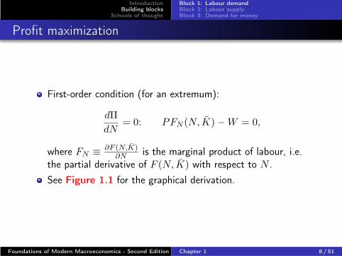
First-order condition (for an extremum):
dΠ
dN= 0: PFN (N, K̄) − W = 0,
where FN ≡ ∂F (N,K̄)∂N is the marginal product of labour, i.e.
the partial derivative of F (N, K̄) with respect to N .
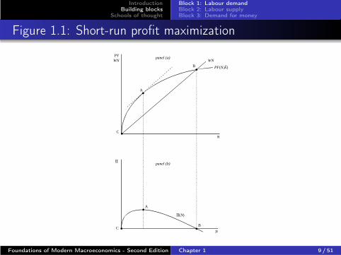
See Figure 1.1 for the graphical derivation.
Foundations of Modern Macroeconomics - Second Edition Chapter 1 8 / 51
IntroductionBuilding blocks
Schools of thought
Block 1: Labour demandBlock 2: Labour supplyBlock 3: Demand for money
Figure 1.1: Short-run profit maximization
!
!
N
WN
B
A
WN
PF(N,K)-
C!
PY
!
!N
B
A
C !
A
A(N)
panel (b)
panel (a)
Foundations of Modern Macroeconomics - Second Edition Chapter 1 9 / 51

IntroductionBuilding blocks
Schools of thought
Block 1: Labour demandBlock 2: Labour supplyBlock 3: Demand for money
Property of the labour demand functionUsing the Implicit Function Theorem
First-order condition is really an “implicit function” relatinglabour demand (ND) to the real wage (W/P ) and the capitalstock (K̄):
PFN (ND, K̄) = W ⇐⇒ FN (ND, K̄) = W/P︸ ︷︷ ︸
real wage
First-year trick comes in handy: total differentiation of theexpression to see how ND, W/P , and K̄ are related:
dFN (ND, K̄) = d(W/P ) ⇒
FNNdND + FNKdK̄ = d(W/P ) ⇒
FNNdND = d(W/P ) − FNKdK̄ ⇒
dND = − (FNK/FNN ) dK̄ + (1/FNN ) d(W/P )
Foundations of Modern Macroeconomics - Second Edition Chapter 1 10 / 51
IntroductionBuilding blocks
Schools of thought
Block 1: Labour demandBlock 2: Labour supplyBlock 3: Demand for money
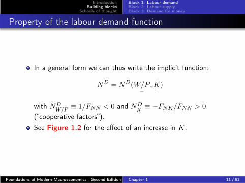
Property of the labour demand function
In a general form we can thus write the implicit function:
ND = ND(W/P−
, K̄+
)
with NDW/P ≡ 1/FNN < 0 and ND
K̄≡ −FNK/FNN > 0
(“cooperative factors”).
See Figure 1.2 for the effect of an increase in K̄.
Foundations of Modern Macroeconomics - Second Edition Chapter 1 11 / 51

IntroductionBuilding blocks
Schools of thought
Block 1: Labour demandBlock 2: Labour supplyBlock 3: Demand for money
Figure 1.2: The demand for labour
N
W/P
ND(W/P, K1)-
ND(W/P, K0)-
Foundations of Modern Macroeconomics - Second Edition Chapter 1 12 / 51
IntroductionBuilding blocks
Schools of thought
Block 1: Labour demandBlock 2: Labour supplyBlock 3: Demand for money
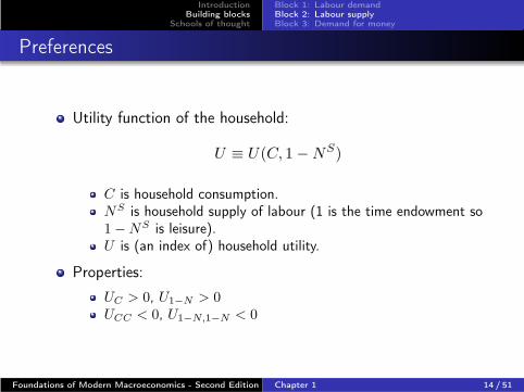
Preferences
Utility function of the household:
U ≡ U(C, 1 − NS)
C is household consumption.NS is household supply of labour (1 is the time endowment so1 − NS is leisure).U is (an index of) household utility.
Properties:
UC > 0, U1−N > 0UCC < 0, U1−N,1−N < 0
Foundations of Modern Macroeconomics - Second Edition Chapter 1 14 / 51

IntroductionBuilding blocks
Schools of thought
Block 1: Labour demandBlock 2: Labour supplyBlock 3: Demand for money
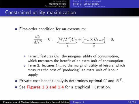
Constrained utility maximization
Budget constraint:P eC = WNS
P e is expected price level (point expectation).Labour income only source of income.
Objective of the household is to choose C and NS tomaximize utility:
max{C,NS}
U ≡ U(C, 1 − NS) subject to P eC = WNS .
Simplified treatment (substitute budget constraint intoobjective function):
max{NS}
U ≡ U[(W/P e)NS , 1 − NS
]
Foundations of Modern Macroeconomics - Second Edition Chapter 1 15 / 51
IntroductionBuilding blocks
Schools of thought
Block 1: Labour demandBlock 2: Labour supplyBlock 3: Demand for money
Constrained utility maximization
First-order condition for an extremum:
dU
dNS= 0 : (W/P e)UC
︸ ︷︷ ︸
1
+ [−1 × U1−N ]︸ ︷︷ ︸
2
= 0.
Term 1 features UC , the marginal utility of consumption,which measures the benefit of an extra unit of consumption.Term 2: features U1−N , the marginal utility of leisure, whichmeasures the cost of “producing” an extra unit of laboursupply.
Private cost-benefit analysis determines optimal C and NS .
See Figures 1.3 and 1.4 for a graphical illustration.
Foundations of Modern Macroeconomics - Second Edition Chapter 1 16 / 51

IntroductionBuilding blocks
Schools of thought
Block 1: Labour demandBlock 2: Labour supplyBlock 3: Demand for money
Figure 1.3: The consumption-leisure choice
U0
C1
!
!
!
E0
E1
EN
10!! ! ! !
C0
CC
C
U1
1!NCS 1!N0
S1!N1S 1!N S
C1S
C0S
!
!
Foundations of Modern Macroeconomics - Second Edition Chapter 1 17 / 51
IntroductionBuilding blocks
Schools of thought
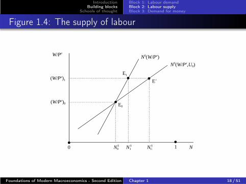
Block 1: Labour demandBlock 2: Labour supplyBlock 3: Demand for money
Figure 1.4: The supply of labour
N
W/Pe
NS(W/Pe)
NS(W/Pe,U0)
(W/Pe)0
(W/Pe)1 !
!
!
E0
E1
EN
10!!
N0S N1
S NCS
Foundations of Modern Macroeconomics - Second Edition Chapter 1 18 / 51
IntroductionBuilding blocks
Schools of thought
Block 1: Labour demandBlock 2: Labour supplyBlock 3: Demand for money
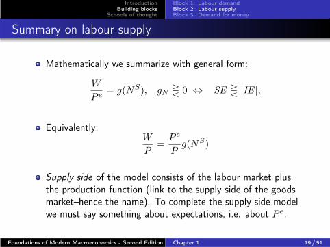
Summary on labour supply
Mathematically we summarize with general form:
W
P e= g(NS), gN R 0 ⇔ SE R |IE |,
Equivalently:W
P=
P e
Pg(NS)
Supply side of the model consists of the labour market plusthe production function (link to the supply side of the goodsmarket–hence the name). To complete the supply side modelwe must say something about expectations, i.e. about P e.
Foundations of Modern Macroeconomics - Second Edition Chapter 1 19 / 51

IntroductionBuilding blocks
Schools of thought
Block 1: Labour demandBlock 2: Labour supplyBlock 3: Demand for money
Expectation Formation Hypotheses
AEH: Adaptive expectations hypothesis:
P et+1 = Pt + (1 − λ)
[P e
t − Pt︸ ︷︷ ︸
(a)
]0 < λ < 1 ⇐⇒
∆P et+1 = λ [Pt − P e
t ] (AEH)
(a): expectational error. P et is given in the short run but it
adjusts slowly over time. If P et > Pt then expectations are
adjusted downwards and vice versa if P et < Pt
PFH: Perfect foresight hypothesis:
P e = P (PFH)
Later in this course we will discuss the rational expectationshypothesis (REH) which is the extension of PFH to thestochastic economy.
Foundations of Modern Macroeconomics - Second Edition Chapter 1 20 / 51
IntroductionBuilding blocks
Schools of thought
Block 1: Labour demandBlock 2: Labour supplyBlock 3: Demand for money
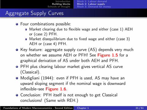
Aggregate Supply Curves
Four combinations possible:Market clearing due to flexible wage and either (case 1) AEHor (case 2) PFH.Market disequilibrium due to fixed wage and either (case 3)AEH or (case 4) PFH.
Key feature: aggregate supply curve (AS) depends very muchon whether we assume AEH or PFH! See Figure 1.5 for agraphical derivation of AS under both AEH and PFH.
PFH plus clearing labour market gives vertical AS curve(Classical).
Modigliani (1944): even if PFH is used, AS may have anupward sloping segment if the nominal wage is downwardinflexible–see Figure 1.6.
Conclusion: PFH itself is not enough to get Classicalconclusions! (Same with REH.)
Foundations of Modern Macroeconomics - Second Edition Chapter 1 21 / 51

IntroductionBuilding blocks
Schools of thought
Block 1: Labour demandBlock 2: Labour supplyBlock 3: Demand for money
Figure 1.5: Aggregate supply and expectations
YN
N Y
Y
PW
Y
W=P1 g(NS)W=P0g(NS)e
W=P2 g(NS)
Y=F(ND, K)-
W=P1FN
W=P2FN
ASPFH
ASAEH
A
BE0
E1
A
A
A
B
B
B
E1
E2E2
E0
E0
E0
P0
P1
P2
W1
W0
W2
N *
Y *
Y1N1 Y2N2
W=P0FN
!!
!
!
!
!
!
!
!
!!
!
!
!
!!
Foundations of Modern Macroeconomics - Second Edition Chapter 1 22 / 51

IntroductionBuilding blocks
Schools of thought
Block 1: Labour demandBlock 2: Labour supplyBlock 3: Demand for money
Figure 1.6: Aggregate supply with downward nominal wage
rigidity
YN
N Y
Y
PW
Y
W=P1 g(NS)
W=P2 g(NS)
Y=F(ND, K)-
W=P1FN
W=P2FN
A
A
A
A
B
E0
E0,B
E0
P0
P1
P2
W1
W0
N *
Y *
Y2N2
W=P0FN
!!
! ! !
!
!
!
!
!
!
C
N* N2S
B
ASW=W0
W=P0 g(NS)
E0,B
Foundations of Modern Macroeconomics - Second Edition Chapter 1 23 / 51

IntroductionBuilding blocks
Schools of thought
Block 1: Labour demandBlock 2: Labour supplyBlock 3: Demand for money
Test your understanding
**** Self Test ****
Derive the AS curve by graphical means under theassumption that the nominal wage cannot fall below W0.Assume that the labour market is initially in equilibriumand that the initial price level is P0.
****
Foundations of Modern Macroeconomics - Second Edition Chapter 1 24 / 51
IntroductionBuilding blocks
Schools of thought
Block 1: Labour demandBlock 2: Labour supplyBlock 3: Demand for money
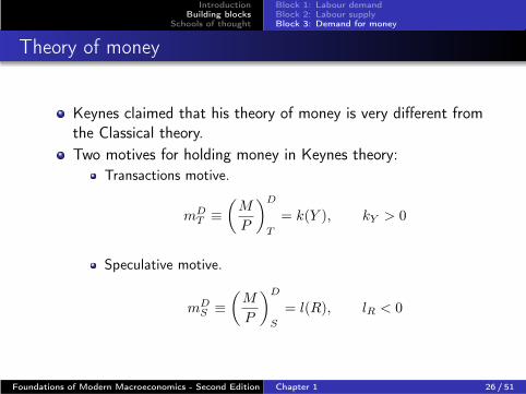
Theory of money
Keynes claimed that his theory of money is very different fromthe Classical theory.
Two motives for holding money in Keynes theory:
Transactions motive.
mDT ≡
(M
P
)D
T
= k(Y ), kY > 0
Speculative motive.
mDS ≡
(M
P
)D
S
= l(R), lR < 0
Foundations of Modern Macroeconomics - Second Edition Chapter 1 26 / 51

IntroductionBuilding blocks
Schools of thought
Block 1: Labour demandBlock 2: Labour supplyBlock 3: Demand for money
Money demand function
Figure 1.7 gives an illustration of a liquidity preferencefunction.
A “liquidity trap” is a distinct possibility: the interest rate is solow (R = RMIN ) that people are indifferent between moneyand bonds. Additional money is willingly absorbed without theneed to lower the interest rate.If R = RMAX then people hold no money for speculativepurposes. Bond prices are very low and are expected to rise.Hence capital gains on bonds are expected.
Foundations of Modern Macroeconomics - Second Edition Chapter 1 27 / 51

IntroductionBuilding blocks
Schools of thought
Block 1: Labour demandBlock 2: Labour supplyBlock 3: Demand for money
Figure 1.7: The liquidity preference function
l(Y,R)
R
l(Y,R)
RMIN
RMAX!
Foundations of Modern Macroeconomics - Second Edition Chapter 1 28 / 51
IntroductionBuilding blocks
Schools of thought
Block 1: Labour demandBlock 2: Labour supplyBlock 3: Demand for money
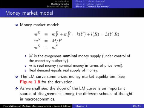
Money market model
Money market model:
mD ≡ mDS + mD
T = k(Y ) + l(R) = L(Y, R)
mS = M/P
mD = mS
M is the exogenous nominal money supply (under control ofthe monetary authority).m is real money (nominal money in terms of price level).Real demand equals real supply of money.
The LM curve summarizes money market equilibrium. SeeFigure 1.8 for the derivation.
As we shall see, the slope of the LM curve is an importantsource of disagreement among the different schools of thoughtin macroeconomics.
Foundations of Modern Macroeconomics - Second Edition Chapter 1 29 / 51

IntroductionBuilding blocks
Schools of thought
Block 1: Labour demandBlock 2: Labour supplyBlock 3: Demand for money
Figure 1.8: Derivation of the LM curve
LM
l(R)
k(Y)Y
!4 < lR < 0
lR 6 !4
lR = 0 !kY/lR 6 4
!kY/lR = 0
!kY/lR > 0RMAX
! !
!
!!
!
!
l(R) + k(Y) = (M/P)0
R
k(Y)
l(R) Y
R
RMIN
l(R)!
!
!
!B1
A1
A2
A3
A4
!
B2
B3
B4
C1C2
C3
C4
!
! !
!D1D2
D3
D4
Foundations of Modern Macroeconomics - Second Edition Chapter 1 30 / 51
IntroductionBuilding blocks
Schools of thought
Block 1: Labour demandBlock 2: Labour supplyBlock 3: Demand for money
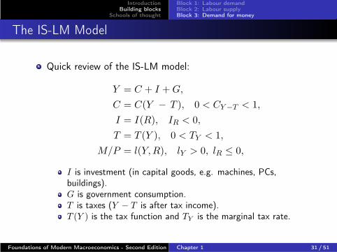
The IS-LM Model
Quick review of the IS-LM model:
Y = C + I + G,
C = C(Y − T ), 0 < CY −T < 1,
I = I(R), IR < 0,
T = T (Y ), 0 < TY < 1,
M/P = l(Y, R), lY > 0, lR ≤ 0,
I is investment (in capital goods, e.g. machines, PCs,buildings).G is government consumption.T is taxes (Y − T is after tax income).T (Y ) is the tax function and TY is the marginal tax rate.
Foundations of Modern Macroeconomics - Second Edition Chapter 1 31 / 51
IntroductionBuilding blocks
Schools of thought
Block 1: Labour demandBlock 2: Labour supplyBlock 3: Demand for money
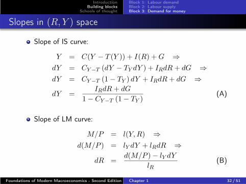
Slopes in (R, Y ) space
Slope of IS curve:
Y = C(Y − T (Y )) + I(R) + G ⇒
dY = CY −T (dY − TY dY ) + IRdR + dG ⇒
dY = CY −T (1 − TY ) dY + IRdR + dG ⇒
dY =IRdR + dG
1 − CY −T (1 − TY )(A)
Slope of LM curve:
M/P = l(Y, R) ⇒
d(M/P ) = lY dY + lRdR ⇒
dR =d(M/P ) − lY dY
lR(B)
Foundations of Modern Macroeconomics - Second Edition Chapter 1 32 / 51
IntroductionBuilding blocks
Schools of thought
Block 1: Labour demandBlock 2: Labour supplyBlock 3: Demand for money
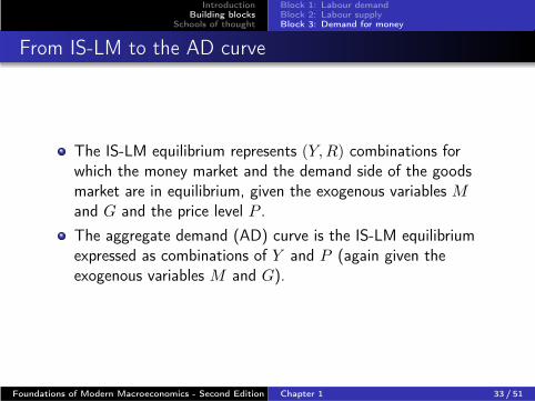
From IS-LM to the AD curve
The IS-LM equilibrium represents (Y, R) combinations forwhich the money market and the demand side of the goodsmarket are in equilibrium, given the exogenous variables Mand G and the price level P .
The aggregate demand (AD) curve is the IS-LM equilibriumexpressed as combinations of Y and P (again given theexogenous variables M and G).
Foundations of Modern Macroeconomics - Second Edition Chapter 1 33 / 51
IntroductionBuilding blocks
Schools of thought
Block 1: Labour demandBlock 2: Labour supplyBlock 3: Demand for money
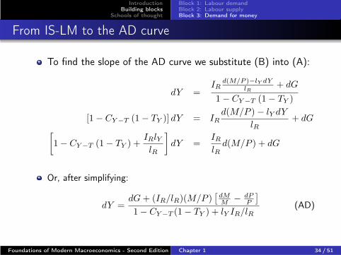
From IS-LM to the AD curve
To find the slope of the AD curve we substitute (B) into (A):
dY =IR
d(M/P )−lY dYlR
+ dG
1 − CY −T (1 − TY )
[1 − CY −T (1 − TY )] dY = IRd(M/P ) − lY dY
lR+ dG
[
1 − CY −T (1 − TY ) +IRlYlR
]
dY =IR
lRd(M/P ) + dG
Or, after simplifying:
dY =dG + (IR/lR)(M/P )
[dMM − dP
P
]
1 − CY −T (1 − TY ) + lY IR/lR(AD)
Foundations of Modern Macroeconomics - Second Edition Chapter 1 34 / 51

IntroductionBuilding blocks
Schools of thought
Block 1: Labour demandBlock 2: Labour supplyBlock 3: Demand for money
Test your understanding
**** Self Test ****
Test your understanding of the material by deriving theAD curve graphically. Pay attention to both the “normal”case (with −∞ < lR < 0) and the liquidity trap case(with lR → −∞)
****
Foundations of Modern Macroeconomics - Second Edition Chapter 1 35 / 51

IntroductionBuilding blocks
Schools of thought
The most important schools of thought
Classical economists
Keynesians
Neo-classical synthesis (a.k.a. neo-Keynesian synthesis)
Monetarists
New-Classical economists
Supply-siders
New-Keynesians
Foundations of Modern Macroeconomics - Second Edition Chapter 1 36 / 51

IntroductionBuilding blocks
Schools of thought
Distinguishing features
The real dividing issues are:
Can the government influence the outcome of the economicprocess?Should the government influence the economic process?
To preview the broad answers:
“Keynesian economists” (broadly defined) generally answer“yes” to both questions.“Classical” economist (broadly defined) generally answer “yes”to the first and “no” to the second question.
Foundations of Modern Macroeconomics - Second Edition Chapter 1 37 / 51

IntroductionBuilding blocks
Schools of thought
Classical Economists
Names: Adam Smith (1723-1790), David Hume (1711-1776),David Ricardo (1772-1823), John Stuart Mill (1806-1873),Knut Wicksell (1851-1926), Irving Fisher (1867-1947).
Quantity theory of money; Fisher’s equation of exchange:
M = kPY
with k constant.
LM curve vertical (lR = 0 in our notation).
AD curve independent of government consumption G .
Foundations of Modern Macroeconomics - Second Edition Chapter 1 38 / 51

IntroductionBuilding blocks
Schools of thought
Classical Economists
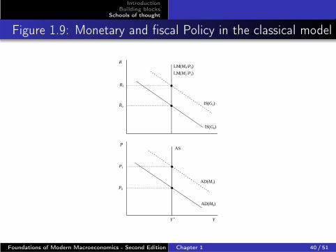
Fiscal policy useless. Just raises interest rate and crowds outinvestment (see Figure 1.9).
Monetary policy useless. Just raises prices and does nothing to“real” things (see Figure 1.9).
Classical dichotomy: money is a veil which determines nominalprices but does not affect real quantities and relative prices.Monetary neutrality.
Conclusion: no need for macroeconomic policy. Leavewell-enough alone. “Laissez-faire” economics.
Foundations of Modern Macroeconomics - Second Edition Chapter 1 39 / 51
IntroductionBuilding blocks
Schools of thought
Figure 1.9: Monetary and fiscal Policy in the classical model
R
P
IS(G1)
IS(G0)
AD(M1)
AD(M0)
LM(M0/P0)
LM(M1/P1)
AS
R1
R0
P0
P1
YY *
!
!
!
!
Foundations of Modern Macroeconomics - Second Edition Chapter 1 40 / 51

IntroductionBuilding blocks
Schools of thought
Keynes?
Names: too many interpreters to mention.
Gimmick of the liquidity trap.
Horizontal segment in the LM curve.
AD curve independent of nominal money supply M .
Classical model is inconsistent! There is no price levelconsistent with full employment. See Figure 1.10.
Foundations of Modern Macroeconomics - Second Edition Chapter 1 41 / 51

IntroductionBuilding blocks
Schools of thought
Keynes?
Fiscal policy very useful. Raises demand (and thus moveseconomy towards full employment); no interest rate changeand thus no crowding out investment (see Figure 1.10).
Monetary policy useless. Does nothing (see Figure 1.10).
But: liquidity trap not relevant in real life and, according toPigou, the real balance effect in consumption will render ADdownward sloping and will ensure logical consistency of theClassical model.
C = C(Y − T+
, M/P+
)
Foundations of Modern Macroeconomics - Second Edition Chapter 1 42 / 51

IntroductionBuilding blocks
Schools of thought
Figure 1.10: Monetary and fiscal policy in the Keynesian
model
R
P
IS(G1)
IS(G0)
LM(M0/P0)
LM(M0/P1)
AD(G0)
P0
P1
Y
!
!!
!
AD(G1)
Y *
AS
!
!
A
A
A
B
B
B
Y0 Y1
RMIN
Foundations of Modern Macroeconomics - Second Edition Chapter 1 43 / 51
IntroductionBuilding blocks
Schools of thought
Neoclassical synthesizers
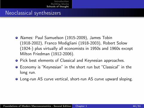
Names: Paul Samuelson (1915-2009), James Tobin(1918-2002), Franco Modigliani (1918-2003), Robert Solow(1924-) plus virtually all economists in 1950s and 1960s exceptMilton Friedman (1912-2006).
Pick best elements of Classical and Keynesian approaches.
Economy is “Keynesian” in the short run but “Classical” in thelong run.
Long-run AS curve vertical, short-run AS curve upward sloping.
Foundations of Modern Macroeconomics - Second Edition Chapter 1 44 / 51

IntroductionBuilding blocks
Schools of thought
Neoclassical synthesizers
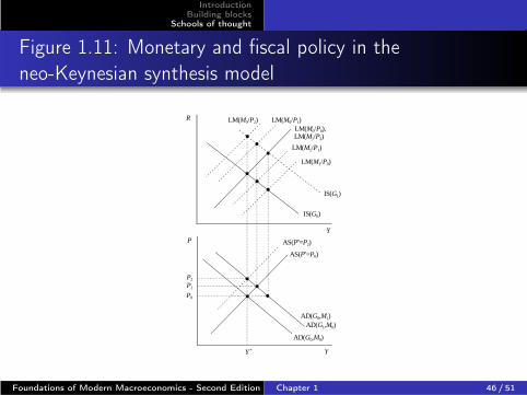
Various sub-species exist, depending on the rationalization ofthe upward sloping short-run AS curve.
Nominal wage, W , sticky downward in the short run.Expected price level, P e, sticky in the short run (adaptiveexpectations).
Both monetary and fiscal policy can affect the economy (seeFigure 1.11).
Underlying presumption is that the government should pursuea counter-cyclical policy.
Foundations of Modern Macroeconomics - Second Edition Chapter 1 45 / 51
IntroductionBuilding blocks
Schools of thought
Figure 1.11: Monetary and fiscal policy in the
neo-Keynesian synthesis model
R
P
IS(G1)
IS(G0)
LM(M0/P0),LM(M0/P1)
AD(G0,M0)
P0
P1
Y
!
!
!
Y *
AS(Pe=P0)
!
!
AD(G0,M1)AD(G1,M0)
AS(Pe=P2)
!
! LM(M1/P1)
LM(M1/P0)
Y
!
!
!P2
LM(M0/P2)
LM(M1/P2)
Foundations of Modern Macroeconomics - Second Edition Chapter 1 46 / 51
IntroductionBuilding blocks
Schools of thought
Monetarists
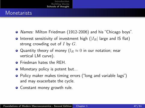
Names: Milton Friedman (1912-2006) and his “Chicago boys”.
Interest sensitivity of investment high (|IR| large and IS flat)strong crowding out of I by G.
Quantity theory of money (lR ≈ 0 in our notation; nearvertical LM curve).
Friedman hates the REH.
Monetary policy is potent but...
Policy maker makes timing errors (“long and variable lags”)and may exacerbate the cycle.
Constant money growth rule.
Foundations of Modern Macroeconomics - Second Edition Chapter 1 47 / 51

IntroductionBuilding blocks
Schools of thought
New Classical economists
Names: Robert Lucas (1937-), Thomas Sargent (1943-),Edward Prescott (1940-), Robert Barro (1944-).
Natural successors to the classical economists.
Flexible prices/wages, REH (or PFH), full employment,efficient markets.
Micro-foundations of macro-relations (e.g. investmentdemand, consumption demand, money demand, labourdemand and supply).
PIP as gimmick early on (see again in Chapter 3).
Foundations of Modern Macroeconomics - Second Edition Chapter 1 48 / 51

IntroductionBuilding blocks
Schools of thought
Supply siders
Names: Arthur Laffer, Robert Mundell (1932-).
Radical conservatives.
Strong distrust of “the government” (Leviathan).
Emphasis on distorting aspects of taxation.
Policy advice too good to be true: you can cut the tax ratewithout reducing government spending. The tax cut pays foritself–see the so-called Laffer curve in Figure 1.12.
Reagan loved it and ran huge deficits! Revisited by Bush Jr.
Are they closet Keynesians?
Foundations of Modern Macroeconomics - Second Edition Chapter 1 49 / 51

IntroductionBuilding blocks
Schools of thought
Figure 1.12: The Laffer curve
10 tL
T
B
A
C
!
!
!
! !
Foundations of Modern Macroeconomics - Second Edition Chapter 1 50 / 51

IntroductionBuilding blocks
Schools of thought
New Keynesian economists
Names: Edmund Phelps (1933-), Stanley Fischer (1943-),John B. Taylor (1946-), Olivier-Jean Blanchard (1948-), GregMankiw (1958-).
Derive their inspiration from John Maynard Keynes.
Markets are prone to fail or to be incomplete.
After initial hesitation acceptance of the REH (or PFH).
Government can and should intervene in the macro-economy.
Keen attention to microfoundations.
Foundations of Modern Macroeconomics - Second Edition Chapter 1 51 / 51