foundations and extensions third editionarslanranjha.weebly.com/uploads/4/8/9/3/4893701/... ·...
TRANSCRIPT

LINEAR PROGRAMMING
Foundations and Extensions
Third Edition

Recent titles in the INTERNATIONAL SERIES IN OPERATIONS RESEARCH & MANAGEMENT SCIENCE Frederick S. Hillier, Series Editor, Stanford University
Sethi, Yan & Zhang/ INVENTORY AND SUPPLY CHAIN MANAGEMENT WITH FORECAST
UPDATES
Cox/ QUANTITATIVE HEALTH RISK ANALYSIS METHODS: Modeling the Human Health Impacts of
Antibiotics Used in Food Animals
Ching & Ng/ MARKOV CHAINS: Models, Algorithms and Applications
Li & Sun/ NONLINEAR INTEGER PROGRAMMING
Kaliszewski/ SOFT COMPUTING FOR COMPLEX MULTIPLE CRITERIA DECISION MAKING
Bouyssou et al/ EVALUATION AND DECISION MODELS WITH MULTIPLE CRITERIA: Stepping
stones for the analyst
Blecker & Friedrich/ MASS CUSTOMIZATION: Challenges and Solutions
Appa, Pitsoulis & Williams/ HANDBOOK ON MODELLING FOR DISCRETE OPTIMIZATION
Herrmann/ HANDBOOK OF PRODUCTION SCHEDULING
Axsäter/ INVENTORY CONTROL, 2nd Ed.
Hall/ PATIENT FLOW: Reducing Delay in Healthcare Delivery
Józefowska & WĊglarz/ PERSPECTIVES IN MODERN PROJECT SCHEDULING
Tian & Zhang/ VACATION QUEUEING MODELS: Theory and Applications
Yan, Yin & Zhang/ STOCHASTIC PROCESSES, OPTIMIZATION, AND CONTROL THEORY
APPLICATIONS IN FINANCIAL ENGINEERING, QUEUEING NETWORKS, AND
MANUFACTURING SYSTEMS
Saaty & Vargas/ DECISION MAKING WITH THE ANALYTIC NETWORK PROCESS: Economic,
Political, Social & Technological Applications w. Benefits, Opportunities, Costs & Risks
Yu/ TECHNOLOGY PORTFOLIO PLANNING AND MANAGEMENT: Practical Concepts and Tools
Kandiller/ PRINCIPLES OF MATHEMATICS IN OPERATIONS RESEARCH
Lee & Lee/ BUILDING SUPPLY CHAIN EXCELLENCE IN EMERGING ECONOMIES
Weintraub/ MANAGEMENT OF NATURAL RESOURCES: A Handbook of Operations Research Models,
Algorithms, and Implementations
Hooker/ INTEGRATED METHODS FOR OPTIMIZATION
Dawande et al/ THROUGHPUT OPTIMIZATION IN ROBOTIC CELLS
Friesz/ NETWORK SCIENCE, NONLINEAR SCIENCE and INFRASTRUCTURE SYSTEMS
Cai, Sha & Wong/ TIME-VARYING NETWORK OPTIMIZATION
Mamon & Elliott/ HIDDEN MARKOV MODELS IN FINANCE
del Castillo/ PROCESS OPTIMIZATION: A Statistical Approach
Józefowska/JUST-IN-TIME SCHEDULING: Models & Algorithms for Computer & Manufacturing
Systems
Yu, Wang & Lai/ FOREIGN-EXCHANGE-RATE FORECASTING WITH ARTIFICIAL NEURAL
NETWORKS
Beyer et al/ MARKOVIAN DEMAND INVENTORY MODELS Shi & Olafsson/ NESTED PARTITIONS OPTIMIZATION: Methodology And Applications Samaniego/ SYSTEM SIGNATURES AND THEIR APPLICATIONS IN ENGINEERING RELIABILITY
Kleijnen/ DESIGN AND ANALYSIS OF SIMULATION EXPERIMENTS
Førsund/ HYDROPOWER ECONOMICS
Kogan & Tapiero/ SUPPLY CHAIN GAMES: Operations Management and Risk Valuation
* A list of the early publications in the series is at the end of the book *
LINEAR PROGRAMMING
Foundations and Extensions
Third Edition
Robert J. Vanderbei Dept. of Operations Research and Financial Engineering
Princeton University, USA
Robert J. Vanderbei
Princeton University
New Jersey, USA
Series Editor:
Fred Hillier
Stanford University
Stanford, CA, USA
ISBN-13: 978-0-387-74387-5 (HB) ISBN-13: 978-0-387-74388-2 (e-book)
Library of Congress Control Number: 2007932884
Printed on acid-free paper.
9 8 7 6 5 4 3 2 1
springer.com
The text for this book was formatted in Times-Roman using AMS-LATEX(which is a macro package for Leslie Lamport’s
LATEX, which itself is a macro package for Donald Knuth’s TEXtext formatting system) and converted to pdf format using
PDFLATEX. The figures were produced using MicroSoft’s POWERPOINT and were incorporated into the text as pdf fileswith the macro package GRAPHICX.TEX.
© 2008 by Robert J. Vanderbei
All rights reserved. This work may not be translated or copied in whole or in part without the written
permission of the publisher (Springer Science+Business Media, LLC, 233 Spring Street, New York, NY
10013, USA), except for brief excerpts in connection with reviews or scholarly analysis. Use in
connection with any form of information storage and retrieval, electronic adaptation, computer software,
or by similar or dissimilar methodology now know or hereafter developed is forbidden.
The use in this publication of trade names, trademarks, service marks and similar terms, even if the are not
identified as such, is not to be taken as an expression of opinion as to whether or not they are subject to
proprietary rights.

To Krisadee,
Marisa and Diana
Contents
Preface xiii
Preface to 2nd Edition xvii
Preface to 3rd Edition xix
Part 1. Basic Theory—The Simplex Method and Duality 1
Chapter 1. Introduction 3
1. Managing a Production Facility 3
2. The Linear Programming Problem 6
Exercises 8
Notes 10
Chapter 2. The Simplex Method 13
1. An Example 13
2. The Simplex Method 16
3. Initialization 19
4. Unboundedness 22
5. Geometry 22
Exercises 24
Notes 27
Chapter 3. Degeneracy 29
1. Definition of Degeneracy 29
2. Two Examples of Degenerate Problems 29
3. The Perturbation/Lexicographic Method 32
4. Bland’s Rule 36
5. Fundamental Theorem of Linear Programming 38
6. Geometry 39
Exercises 42
Notes 43
Chapter 4. Efficiency of the Simplex Method 45
vii
viii CONTENTS
1. Performance Measures 45
2. Measuring the Size of a Problem 45
3. Measuring the Effort to Solve a Problem 46
4. Worst-Case Analysis of the Simplex Method 47
Exercises 52
Notes 53
Chapter 5. Duality Theory 55
1. Motivation—Finding Upper Bounds 55
2. The Dual Problem 57
3. The Weak Duality Theorem 58
4. The Strong Duality Theorem 60
5. Complementary Slackness 66
6. The Dual Simplex Method 68
7. A Dual-Based Phase I Algorithm 71
8. The Dual of a Problem in General Form 73
9. Resource Allocation Problems 74
10. Lagrangian Duality 78
Exercises 79
Notes 87
Chapter 6. The Simplex Method in Matrix Notation 89
1. Matrix Notation 89
2. The Primal Simplex Method 91
3. An Example 96
4. The Dual Simplex Method 101
5. Two-Phase Methods 104
6. Negative Transpose Property 105
Exercises 108
Notes 109
Chapter 7. Sensitivity and Parametric Analyses 111
1. Sensitivity Analysis 111
2. Parametric Analysis and the Homotopy Method 115
3. The Parametric Self-Dual Simplex Method 119
Exercises 120
Notes 124
Chapter 8. Implementation Issues 125
1. Solving Systems of Equations: LU -Factorization 126
2. Exploiting Sparsity 130
3. Reusing a Factorization 136
4. Performance Tradeoffs 140

CONTENTS ix
5. Updating a Factorization 141
6. Shrinking the Bump 145
7. Partial Pricing 146
8. Steepest Edge 147
Exercises 149
Notes 150
Chapter 9. Problems in General Form 151
1. The Primal Simplex Method 151
2. The Dual Simplex Method 153
Exercises 159
Notes 160
Chapter 10. Convex Analysis 161
1. Convex Sets 161
2. Caratheodory’s Theorem 163
3. The Separation Theorem 165
4. Farkas’ Lemma 167
5. Strict Complementarity 168
Exercises 170
Notes 171
Chapter 11. Game Theory 173
1. Matrix Games 173
2. Optimal Strategies 175
3. The Minimax Theorem 177
4. Poker 181
Exercises 184
Notes 187
Chapter 12. Regression 189
1. Measures of Mediocrity 189
2. Multidimensional Measures: Regression Analysis 191
3. L2-Regression 193
4. L1-Regression 195
5. Iteratively Reweighted Least Squares 196
6. An Example: How Fast is the Simplex Method? 198
7. Which Variant of the Simplex Method is Best? 202
Exercises 203
Notes 208
Chapter 13. Financial Applications 211
1. Portfolio Selection 211
x CONTENTS
2. Option Pricing 216
Exercises 221
Notes 222
Part 2. Network-Type Problems 223
Chapter 14. Network Flow Problems 225
1. Networks 225
2. Spanning Trees and Bases 228
3. The Primal Network Simplex Method 233
4. The Dual Network Simplex Method 237
5. Putting It All Together 240
6. The Integrality Theorem 243
Exercises 244
Notes 252
Chapter 15. Applications 253
1. The Transportation Problem 253
2. The Assignment Problem 255
3. The Shortest-Path Problem 256
4. Upper-Bounded Network Flow Problems 259
5. The Maximum-Flow Problem 262
Exercises 264
Notes 269
Chapter 16. Structural Optimization 271
1. An Example 271
2. Incidence Matrices 273
3. Stability 274
4. Conservation Laws 276
5. Minimum-Weight Structural Design 279
6. Anchors Away 281
Exercises 284
Notes 284
Part 3. Interior-Point Methods 287
Chapter 17. The Central Path 289
Warning: Nonstandard Notation Ahead 289
1. The Barrier Problem 289
2. Lagrange Multipliers 292
3. Lagrange Multipliers Applied to the Barrier Problem 295
4. Second-Order Information 297
CONTENTS xi
5. Existence 297
Exercises 299
Notes 301
Chapter 18. A Path-Following Method 303
1. Computing Step Directions 303
2. Newton’s Method 305
3. Estimating an Appropriate Value for the Barrier Parameter 306
4. Choosing the Step Length Parameter 307
5. Convergence Analysis 308
Exercises 314
Notes 318
Chapter 19. The KKT System 319
1. The Reduced KKT System 319
2. The Normal Equations 320
3. Step Direction Decomposition 322
Exercises 325
Notes 325
Chapter 20. Implementation Issues 327
1. Factoring Positive Definite Matrices 327
2. Quasidefinite Matrices 331
3. Problems in General Form 337
Exercises 342
Notes 342
Chapter 21. The Affine-Scaling Method 345
1. The Steepest Ascent Direction 345
2. The Projected Gradient Direction 347
3. The Projected Gradient Direction with Scaling 349
4. Convergence 353
5. Feasibility Direction 355
6. Problems in Standard Form 356
Exercises 357
Notes 358
Chapter 22. The Homogeneous Self-Dual Method 361
1. From Standard Form to Self-Dual Form 361
2. Homogeneous Self-Dual Problems 362
3. Back to Standard Form 372
4. Simplex Method vs Interior-Point Methods 375
Exercises 379
xii CONTENTS
Notes 380
Part 4. Extensions 383
Chapter 23. Integer Programming 385
1. Scheduling Problems 385
2. The Traveling Salesman Problem 387
3. Fixed Costs 390
4. Nonlinear Objective Functions 390
5. Branch-and-Bound 392
Exercises 404
Notes 405
Chapter 24. Quadratic Programming 407
1. The Markowitz Model 407
2. The Dual 412
3. Convexity and Complexity 414
4. Solution Via Interior-Point Methods 418
5. Practical Considerations 419
Exercises 422
Notes 423
Chapter 25. Convex Programming 425
1. Differentiable Functions and Taylor Approximations 425
2. Convex and Concave Functions 426
3. Problem Formulation 426
4. Solution Via Interior-Point Methods 427
5. Successive Quadratic Approximations 429
6. Merit Functions 429
7. Parting Words 433
Exercises 433
Notes 435
Appendix A. Source Listings 437
1. The Self-Dual Simplex Method 438
2. The Homogeneous Self-Dual Method 441
Answers to Selected Exercises 445
Bibliography 449
Index 457

Preface
This book is about constrained optimization. It begins with a thorough treatment
of linear programming and proceeds to convex analysis, network flows, integer pro-
gramming, quadratic programming, and convex optimization. Along the way, dynamic
programming and the linear complementarity problem are touched on as well.
The book aims to be a first introduction to the subject. Specific examples and
concrete algorithms precede more abstract topics. Nevertheless, topics covered are
developed in some depth, a large number of numerical examples are worked out in
detail, and many recent topics are included, most notably interior-point methods. The
exercises at the end of each chapter both illustrate the theory and, in some cases, extend
it.
Prerequisites. The book is divided into four parts. The first two parts assume a
background only in linear algebra. For the last two parts, some knowledge of multi-
variate calculus is necessary. In particular, the student should know how to use La-
grange multipliers to solve simple calculus problems in 2 and 3 dimensions.
Associated software. It is good to be able to solve small problems by hand, but the
problems one encounters in practice are large, requiring a computer for their solution.
Therefore, to fully appreciate the subject, one needs to solve large (practical) prob-
lems on a computer. An important feature of this book is that it comes with software
implementing the major algorithms described herein. At the time of writing, software
for the following five algorithms is available:
• The two-phase simplex method as shown in Figure 6.1.
• The self-dual simplex method as shown in Figure 7.1.
• The path-following method as shown in Figure 18.1.
• The homogeneous self-dual method as shown in Figure 22.1.
• The long-step homogeneous self-dual method as described in Exercise 22.4.
The programs that implement these algorithms are written in C and can be easily
compiled on most hardware platforms. Students/instructors are encouraged to install
and compile these programs on their local hardware. Great pains have been taken to
make the source code for these programs readable (see Appendix A). In particular, the
names of the variables in the programs are consistent with the notation of this book.
There are two ways to run these programs. The first is to prepare the input in a
standard computer-file format, called MPS format, and to run the program using such
xiii
xiv PREFACE
a file as input. The advantage of this input format is that there is an archive of problems
stored in this format, called the NETLIB suite, that one can download and use imme-
diately (a link to the NETLIB suite can be found at the web site mentioned below).
But, this format is somewhat archaic and, in particular, it is not easy to create these
files by hand. Therefore, the programs can also be run from within a problem model-
ing system called AMPL. AMPL allows one to describe mathematical programming
problems using an easy to read, yet concise, algebraic notation. To run the programs
within AMPL, one simply tells AMPL the name of the solver-program before asking
that a problem be solved. The text that describes AMPL, (Fourer et al. 1993), makes
an excellent companion to this book. It includes a discussion of many practical linear
programming problems. It also has lots of exercises to hone the modeling skills of the
student.
Several interesting computer projects can be suggested. Here are a few sugges-
tions regarding the simplex codes:
• Incorporate the partial pricing strategy (see Section 8.7) into the two-phase
simplex method and compare it with full pricing.
• Incorporate the steepest-edge pivot rule (see Section 8.8) into the two-phase
simplex method and compare it with the largest-coefficient rule.
• Modify the code for either variant of the simplex method so that it can treat
bounds and ranges implicitly (see Chapter 9), and compare the performance
with the explicit treatment of the supplied codes.
• Implement a “warm-start” capability so that the sensitivity analyses dis-
cussed in Chapter 7 can be done.
• Extend the simplex codes to be able to handle integer programming prob-
lems using the branch-and-bound method described in Chapter 23.
As for the interior-point codes, one could try some of the following projects:
• Modify the code for the path-following algorithm so that it implements the
affine-scaling method (see Chapter 21), and then compare the two methods.
• Modify the code for the path-following method so that it can treat bounds
and ranges implicitly (see Section 20.3), and compare the performance against
the explicit treatment in the given code.
• Modify the code for the path-following method to implement the higher-
order method described in Exercise 18.5. Compare.
• Extend the path-following code to solve quadratic programming problems
using the algorithm shown in Figure 24.3.
• Further extend the code so that it can solve convex optimization problems
using the algorithm shown in Figure 25.2.
And, perhaps the most interesting project of all:
• Compare the simplex codes against the interior-point code and decide for
yourself which algorithm is better on specific families of problems.
PREFACE xv
The software implementing the various algorithms was developed using consistent
data structures and so making fair comparisons should be straightforward. The soft-
ware can be downloaded from the following web site:
http://www.princeton.edu/∼rvdb/LPbook/
If, in the future, further codes relating to this text are developed (for example, a self-
dual network simplex code), they will be made available through this web site.
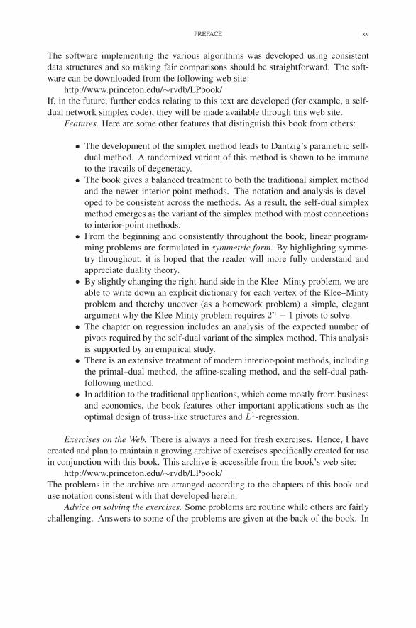
Features. Here are some other features that distinguish this book from others:
• The development of the simplex method leads to Dantzig’s parametric self-
dual method. A randomized variant of this method is shown to be immune
to the travails of degeneracy.
• The book gives a balanced treatment to both the traditional simplex method
and the newer interior-point methods. The notation and analysis is devel-
oped to be consistent across the methods. As a result, the self-dual simplex
method emerges as the variant of the simplex method with most connections
to interior-point methods.
• From the beginning and consistently throughout the book, linear program-
ming problems are formulated in symmetric form. By highlighting symme-
try throughout, it is hoped that the reader will more fully understand and
appreciate duality theory.
• By slightly changing the right-hand side in the Klee–Minty problem, we are
able to write down an explicit dictionary for each vertex of the Klee–Minty
problem and thereby uncover (as a homework problem) a simple, elegant
argument why the Klee-Minty problem requires 2n − 1 pivots to solve.
• The chapter on regression includes an analysis of the expected number of
pivots required by the self-dual variant of the simplex method. This analysis
is supported by an empirical study.
• There is an extensive treatment of modern interior-point methods, including
the primal–dual method, the affine-scaling method, and the self-dual path-
following method.
• In addition to the traditional applications, which come mostly from business
and economics, the book features other important applications such as the
optimal design of truss-like structures and L1-regression.
Exercises on the Web. There is always a need for fresh exercises. Hence, I have
created and plan to maintain a growing archive of exercises specifically created for use
in conjunction with this book. This archive is accessible from the book’s web site:
http://www.princeton.edu/∼rvdb/LPbook/
The problems in the archive are arranged according to the chapters of this book and
use notation consistent with that developed herein.
Advice on solving the exercises. Some problems are routine while others are fairly
challenging. Answers to some of the problems are given at the back of the book. In

xvi PREFACE
general, the advice given to me by Leonard Gross (when I was a student) should help
even on the hard problems: follow your nose.
Audience. This book evolved from lecture notes developed for my introduc-
tory graduate course in linear programming as well as my upper-level undergradu-
ate course. A reasonable undergraduate syllabus would cover essentially all of Part 1
(Simplex Method and Duality), the first two chapters of Part 2 (Network Flows and
Applications), and the first chapter of Part 4 (Integer Programming). At the gradu-
ate level, the syllabus should depend on the preparation of the students. For a well-
prepared class, one could cover the material in Parts 1 and 2 fairly quickly and then
spend more time on Parts 3 (Interior-Point Methods) and 4 (Extensions).
Dependencies. In general, Parts 2 and 3 are completely independent of each other.
Both depend, however, on the material in Part 1. The first Chapter in Part 4 (Integer
Programming) depends only on material from Part 1, whereas the remaining chapters
build on Part 3 material.
Acknowledgments. My interest in linear programming was sparked by Robert
Garfinkel when we shared an office at Bell Labs. I would like to thank him for
his constant encouragement, advice, and support. This book benefited greatly from
the thoughtful comments and suggestions of David Bernstein and Michael Todd. I
would also like to thank the following colleagues for their help: Ronny Ben-Tal, Leslie
Hall, Yoshi Ikura, Victor Klee, Irvin Lustig, Avi Mandelbaum, Marc Meketon, Narcis
Nabona, James Orlin, Andrzej Ruszczynski, and Henry Wolkowicz. I would like to
thank Gary Folven at Kluwer and Fred Hillier, the series editor, for encouraging me to
undertake this project. I would like to thank my students for finding many typos and
occasionally more serious errors: John Gilmartin, Jacinta Warnie, Stephen Woolbert,
Lucia Wu, and Bing Yang My thanks to Erhan Cınlar for the many times he offered
advice on questions of style. I hope this book reflects positively on his advice. Finally,
I would like to acknowledge the support of the National Science Foundation and the
Air Force Office of Scientific Research for supporting me while writing this book. In
a time of declining resources, I am especially grateful for their support.
Robert J. Vanderbei
September, 1996
Preface to 2nd Edition
For the 2nd edition, many new exercises have been added. Also I have worked
hard to develop online tools to aid in learning the simplex method and duality theory.
These online tools can be found on the book’s web page:
http://www.princeton.edu/∼rvdb/LPbook/
and are mentioned at appropriate places in the text. Besides the learning tools, I have
created several online exercises. These exercises use randomly generated problems
and therefore represent a virtually unlimited collection of “routine” exercises that can
be used to test basic understanding. Pointers to these online exercises are included in
the exercises sections at appropriate points.
Some other notable changes include:
• The chapter on network flows has been completely rewritten. Hopefully, the
new version is an improvement on the original.
• Two different fonts are now used to distinguish between the set of basic
indices and the basis matrix.
• The first edition placed great emphasis on the symmetry between the primal
and the dual (the negative transpose property). The second edition carries
this further with a discussion of the relationship between the basic and non-
basic matrices B and N as they appear in the primal and in the dual. We
show that, even though these matrices differ (they even have different di-
mensions), B−1N in the dual is the negative transpose of the corresponding
matrix in the primal.
• In the chapters devoted to the simplex method in matrix notation, the collec-
tion of variables z1, z2, . . . , zn, y1, y2, . . . , ym was replaced, in the first edi-
tion, with the single array of variables y1, y2, . . . , yn+m. This caused great
confusion as the variable yi in the original notation was changed to yn+i in
the new notation. For the second edition, I have changed the notation for the
single array to z1, z2, . . . , zn+m.
• A number of figures have been added to the chapters on convex analysis and
on network flow problems.
xvii

xviii PREFACE TO 2ND EDITION
• The algorithm refered to as the primal–dual simplex method in the first edi-
tion has been renamed the parametric self-dual simplex method in accor-
dance with prior standard usage.
• The last chapter, on convex optimization, has been extended with a discus-
sion of merit functions and their use in shortenning steps to make some
otherwise nonconvergent problems converge.
Acknowledgments. Many readers have sent corrections and suggestions for im-
provement. Many of the corrections were incorporated into earlier reprintings. Only
those that affected pagination were accrued to this new edition. Even though I cannot
now remember everyone who wrote, I am grateful to them all. Some sent comments
that had significant impact. They were Hande Benson, Eric Denardo, Sudhakar Man-
dapati, Michael Overton, and Jos Sturm.
Robert J. Vanderbei
December, 2000
Preface to 3rd Edition
It has been almost seven years since the 2nd edition appeared and the publisher is
itching for me to finish a new edition. The previous edition had very few typos. I have
fixed them all! Of course, I’ve also added some new material and who knows how
many new typos I’ve introduced. The most significant new material is contained in a
new chapter on financial applications, which discusses a linear programming variant of
the portfolio selection problem and option pricing. I am grateful to Alex d’Aspremont
for pointing out that the option pricing problem provides a nice application of duality
theory. Finally, I’d like to acknowledge the fact that half (four out of eight) of the
typos were reported to me by Trond Steihaug. Thanks Trond!
Robert J. Vanderbei
June, 2007
xix

CHAPTER 1
Introduction
This book is mostly about a subject called Linear Programming. Before defining
what we mean, in general, by a linear programming problem, let us describe a few
practical real-world problems that serve to motivate and at least vaguely to define this
subject.
1. Managing a Production Facility
Consider a production facility for a manufacturing company. The facility is ca-
pable of producing a variety of products that, for simplicity, we shall enumerate as
1, 2, . . . , n. These products are constructed/manufactured/produced out of certain raw
materials. Let us assume that there are m different raw materials, which again we shall
simply enumerate as 1, 2, . . . , m. The decisions involved in managing/operating this
facility are complicated and arise dynamically as market conditions evolve around it.
However, to describe a simple, fairly realistic optimization problem, we shall consider
a particular snapshot of the dynamic evolution. At this specific point in time, the fa-
cility has, for each raw material i = 1, 2, . . . ,m, a known amount, say bi, on hand.
Furthermore, each raw material has at this moment in time a known unit market value.
We shall denote the unit value of the ith raw material by ρi.
In addition, each product is made from known amounts of the various raw materi-
als. That is, producing one unit of product j requires a certain known amount, say aij
units, of raw material i. Also, the jth final product can be sold at the known prevailing
market price of σj dollars per unit.
Throughout this section we make an important assumption:
The production facility is small relative to the market as a whole
and therefore cannot through its actions alter the prevailing market
value of its raw materials, nor can it affect the prevailing market
price for its products.
We shall consider two optimization problems related to the efficient operation of
this facility (later, in Chapter 5, we shall see that these two problems are in fact closely
related to each other).
1.1. Production Manager as Optimist. The first problem we wish to consider
is the one faced by the company’s production manager. It is the problem of how to use
3
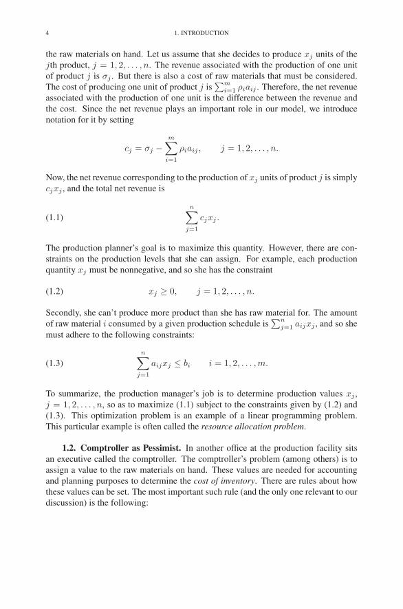
4 1. INTRODUCTION
the raw materials on hand. Let us assume that she decides to produce xj units of the
jth product, j = 1, 2, . . . , n. The revenue associated with the production of one unit
of product j is σj . But there is also a cost of raw materials that must be considered.
The cost of producing one unit of product j is∑m
i=1 ρiaij . Therefore, the net revenue
associated with the production of one unit is the difference between the revenue and
the cost. Since the net revenue plays an important role in our model, we introduce
notation for it by setting
cj = σj −m∑
i=1
ρiaij , j = 1, 2, . . . , n.
Now, the net revenue corresponding to the production of xj units of product j is simply
cjxj , and the total net revenue is
(1.1)
n∑
j=1
cjxj .
The production planner’s goal is to maximize this quantity. However, there are con-
straints on the production levels that she can assign. For example, each production
quantity xj must be nonnegative, and so she has the constraint
(1.2) xj ≥ 0, j = 1, 2, . . . , n.
Secondly, she can’t produce more product than she has raw material for. The amount
of raw material i consumed by a given production schedule is∑n
j=1 aijxj , and so she
must adhere to the following constraints:
(1.3)
n∑
j=1
aijxj ≤ bi i = 1, 2, . . . ,m.
To summarize, the production manager’s job is to determine production values xj ,
j = 1, 2, . . . , n, so as to maximize (1.1) subject to the constraints given by (1.2) and
(1.3). This optimization problem is an example of a linear programming problem.
This particular example is often called the resource allocation problem.
1.2. Comptroller as Pessimist. In another office at the production facility sits
an executive called the comptroller. The comptroller’s problem (among others) is to
assign a value to the raw materials on hand. These values are needed for accounting
and planning purposes to determine the cost of inventory. There are rules about how
these values can be set. The most important such rule (and the only one relevant to our
discussion) is the following:
1. MANAGING A PRODUCTION FACILITY 5
The company must be willing to sell the raw materials should an
outside firm offer to buy them at a price consistent with these
values.
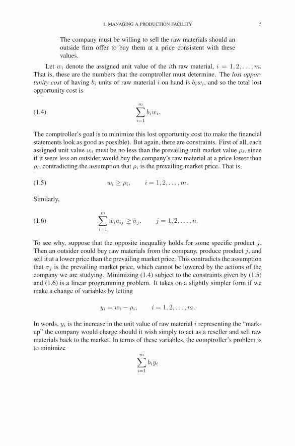
Let wi denote the assigned unit value of the ith raw material, i = 1, 2, . . . ,m.
That is, these are the numbers that the comptroller must determine. The lost oppor-
tunity cost of having bi units of raw material i on hand is biwi, and so the total lost
opportunity cost is
(1.4)
m∑
i=1
biwi.
The comptroller’s goal is to minimize this lost opportunity cost (to make the financial
statements look as good as possible). But again, there are constraints. First of all, each
assigned unit value wi must be no less than the prevailing unit market value ρi, since
if it were less an outsider would buy the company’s raw material at a price lower than
ρi, contradicting the assumption that ρi is the prevailing market price. That is,
(1.5) wi ≥ ρi, i = 1, 2, . . . ,m.
Similarly,
(1.6)
m∑
i=1
wiaij ≥ σj , j = 1, 2, . . . , n.
To see why, suppose that the opposite inequality holds for some specific product j.
Then an outsider could buy raw materials from the company, produce product j, and
sell it at a lower price than the prevailing market price. This contradicts the assumption
that σj is the prevailing market price, which cannot be lowered by the actions of the
company we are studying. Minimizing (1.4) subject to the constraints given by (1.5)
and (1.6) is a linear programming problem. It takes on a slightly simpler form if we
make a change of variables by letting
yi = wi − ρi, i = 1, 2, . . . ,m.
In words, yi is the increase in the unit value of raw material i representing the “mark-
up” the company would charge should it wish simply to act as a reseller and sell raw
materials back to the market. In terms of these variables, the comptroller’s problem is
to minimizem∑
i=1
biyi

6 1. INTRODUCTION
subject tom∑
i=1
yiaij ≥ cj , j = 1, 2, . . . , n
and
yi ≥ 0, i = 1, 2, . . . ,m.
Note that we’ve dropped a term,∑m
i=1 biρi, from the objective. It is a constant (the
market value of the raw materials), and so, while it affects the value of the function
being minimized, it does not have any impact on the actual optimal values of the
variables (whose determination is the comptroller’s main interest).
2. The Linear Programming Problem
In the two examples given above, there have been variables whose values are to be
decided in some optimal fashion. These variables are referred to as decision variables.
They are usually written as
xj , j = 1, 2, . . . , n.
In linear programming, the objective is always to maximize or to minimize some linear
function of these decision variables
ζ = c1x1 + c2x2 + · · · + cnxn.
This function is called the objective function. It often seems that real-world prob-
lems are most naturally formulated as minimizations (since real-world planners al-
ways seem to be pessimists), but when discussing mathematics it is usually nicer to
work with maximization problems. Of course, converting from one to the other is triv-
ial both from the modeler’s viewpoint (either minimize cost or maximize profit) and
from the analyst’s viewpoint (either maximize ζ or minimize −ζ). Since this book is
primarily about the mathematics of linear programming, we shall usually consider our
aim one of maximizing the objective function.
In addition to the objective function, the examples also had constraints. Some
of these constraints were really simple, such as the requirement that some decision
variable be nonnegative. Others were more involved. But in all cases the constraints
consisted of either an equality or an inequality associated with some linear combina-
tion of the decision variables:
a1x1 + a2x2 + · · · + anxn
⎧
⎪
⎪
⎨
⎪
⎪
⎩
≤=
≥
⎫
⎪
⎪
⎬
⎪
⎪
⎭
b.

2. THE LINEAR PROGRAMMING PROBLEM 7
It is easy to convert constraints from one form to another. For example, an in-
equality constraint
a1x1 + a2x2 + · · · + anxn ≤ b
can be converted to an equality constraint by adding a nonnegative variable, w, which
we call a slack variable:
a1x1 + a2x2 + · · · + anxn + w = b, w ≥ 0.
On the other hand, an equality constraint
a1x1 + a2x2 + · · · + anxn = b
can be converted to inequality form by introducing two inequality constraints:
a1x1 + a2x2 + · · · + anxn ≤ b
a1x1 + a2x2 + · · · + anxn ≥ b.
Hence, in some sense, there is no a priori preference for how one poses the constraints
(as long as they are linear, of course). However, we shall also see that, from a math-
ematical point of view, there is a preferred presentation. It is to pose the inequalities
as less-thans and to stipulate that all the decision variables be nonnegative. Hence, the
linear programming problem as we shall study it can be formulated as follows:
maximize c1x1 + c2x2 + · · ·+ cnxn
subject to a11x1 + a12x2 + · · ·+ a1nxn ≤ b1
a21x1 + a22x2 + · · ·+ a2nxn ≤ b2
...
am1x1 + am2x2 + · · ·+ amnxn ≤ bm
x1, x2, . . . xn ≥ 0.
We shall refer to linear programs formulated this way as linear programs in standard
form. We shall always use m to denote the number of constraints, and n to denote the
number of decision variables.
A proposal of specific values for the decision variables is called a solution. A
solution (x1, x2, . . . , xn) is called feasible if it satisfies all of the constraints. It is
called optimal if in addition it attains the desired maximum. Some problems are just

8 1. INTRODUCTION
simply infeasible, as the following example illustrates:
maximize 5x1 + 4x2
subject to x1 + x2 ≤ 2
−2x1 − 2x2 ≤−9
x1, x2 ≥ 0.
Indeed, the second constraint implies that x1 + x2 ≥ 4.5, which contradicts the first
constraint. If a problem has no feasible solution, then the problem itself is called
infeasible.
At the other extreme from infeasible problems, one finds unbounded problems.
A problem is unbounded if it has feasible solutions with arbitrarily large objective
values. For example, consider
maximize x1 − 4x2
subject to −2x1 + x2 ≤−1
−x1 − 2x2 ≤−2
x1, x2 ≥ 0.
Here, we could set x2 to zero and let x1 be arbitrarily large. As long as x1 is greater
than 2 the solution will be feasible, and as it gets large the objective function does too.
Hence, the problem is unbounded. In addition to finding optimal solutions to linear
programming problems, we shall also be interested in detecting when a problem is
infeasible or unbounded.
Exercises
1.1 A steel company must decide how to allocate next week’s time on a rolling
mill, which is a machine that takes unfinished slabs of steel as input and can
produce either of two semi-finished products: bands and coils. The mill’s
two products come off the rolling line at different rates:
Bands 200 tons/hr
Coils 140 tons/hr .
They also produce different profits:
Bands $ 25/ton
Coils $ 30/ton .
Based on currently booked orders, the following upper bounds are placed on
the amount of each product to produce:
EXERCISES 9
Bands 6000 tons
Coils 4000 tons .
Given that there are 40 hours of production time available this week, the
problem is to decide how many tons of bands and how many tons of coils
should be produced to yield the greatest profit. Formulate this problem as a
linear programming problem. Can you solve this problem by inspection?
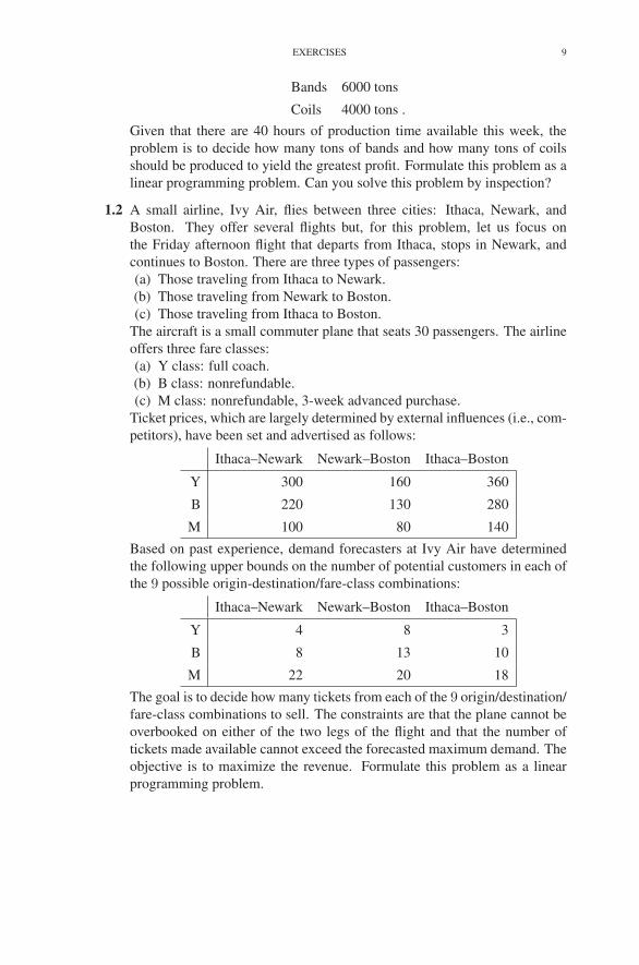
1.2 A small airline, Ivy Air, flies between three cities: Ithaca, Newark, and
Boston. They offer several flights but, for this problem, let us focus on
the Friday afternoon flight that departs from Ithaca, stops in Newark, and
continues to Boston. There are three types of passengers:
(a) Those traveling from Ithaca to Newark.
(b) Those traveling from Newark to Boston.
(c) Those traveling from Ithaca to Boston.
The aircraft is a small commuter plane that seats 30 passengers. The airline
offers three fare classes:
(a) Y class: full coach.
(b) B class: nonrefundable.
(c) M class: nonrefundable, 3-week advanced purchase.
Ticket prices, which are largely determined by external influences (i.e., com-
petitors), have been set and advertised as follows:
Ithaca–Newark Newark–Boston Ithaca–Boston
Y 300 160 360
B 220 130 280
M 100 80 140
Based on past experience, demand forecasters at Ivy Air have determined
the following upper bounds on the number of potential customers in each of
the 9 possible origin-destination/fare-class combinations:
Ithaca–Newark Newark–Boston Ithaca–Boston
Y 4 8 3
B 8 13 10
M 22 20 18
The goal is to decide how many tickets from each of the 9 origin/destination/
fare-class combinations to sell. The constraints are that the plane cannot be
overbooked on either of the two legs of the flight and that the number of
tickets made available cannot exceed the forecasted maximum demand. The
objective is to maximize the revenue. Formulate this problem as a linear
programming problem.
10 1. INTRODUCTION
1.3 Suppose that Y is a random variable taking on one of n known values:
a1, a2, . . . , an.
Suppose we know that Y either has distribution p given by
P(Y = aj) = pj
or it has distribution q given by
P(Y = aj) = qj .
Of course, the numbers pj , j = 1, 2, . . . , n are nonnegative and sum to
one. The same is true for the qj’s. Based on a single observation of Y ,
we wish to guess whether it has distribution p or distribution q. That is,
for each possible outcome aj , we will assert with probability xj that the
distribution is p and with probability 1−xj that the distribution is q. We wish
to determine the probabilities xj , j = 1, 2, . . . , n, such that the probability
of saying the distribution is p when in fact it is q has probability no larger
than β, where β is some small positive value (such as 0.05). Furthermore,
given this constraint, we wish to maximize the probability that we say the
distribution is p when in fact it is p. Formulate this maximization problem
as a linear programming problem.
Notes
The subject of linear programming has its roots in the study of linear inequali-
ties, which can be traced as far back as 1826 to the work of Fourier. Since then, many
mathematicians have proved special cases of the most important result in the subject—
the duality theorem. The applied side of the subject got its start in 1939 when L.V.
Kantorovich noted the practical importance of a certain class of linear programming
problems and gave an algorithm for their solution—see Kantorovich (1960). Unfortu-
nately, for several years, Kantorovich’s work was unknown in the West and unnoticed
in the East. The subject really took off in 1947 when G.B. Dantzig invented the simplex
method for solving the linear programming problems that arose in U.S. Air Force plan-
ning problems. The earliest published accounts of Dantzig’s work appeared in 1951
(Dantzig 1951a,b). His monograph (Dantzig 1963) remains an important reference. In
the same year that Dantzig invented the simplex method, T.C. Koopmans showed that
linear programming provided the appropriate model for the analysis of classical eco-
nomic theories. In 1975, the Royal Swedish Academy of Sciences awarded the Nobel
Prize in economic science to L.V. Kantorovich and T.C. Koopmans “for their contri-
butions to the theory of optimum allocation of resources.” Apparently the academy
regarded Dantzig’s work as too mathematical for the prize in economics (and there is
no Nobel Prize in mathematics).

NOTES 11
The textbooks by Bradley et al. (1977), Bazaraa et al. (1977), and Hillier &
Lieberman (1977) are known for their extensive collections of interesting practical
applications.

CHAPTER 2
The Simplex Method
In this chapter we present the simplex method as it applies to linear programming
problems in standard form.
1. An Example
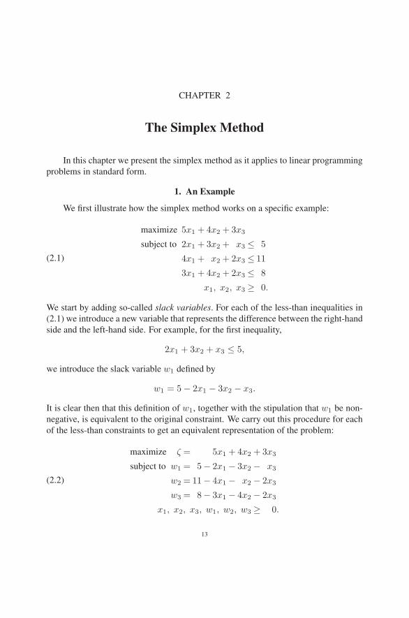
We first illustrate how the simplex method works on a specific example:
(2.1)
maximize 5x1 + 4x2 + 3x3
subject to 2x1 + 3x2 + x3 ≤ 5
4x1 + x2 + 2x3 ≤ 11
3x1 + 4x2 + 2x3 ≤ 8
x1, x2, x3 ≥ 0.
We start by adding so-called slack variables. For each of the less-than inequalities in
(2.1) we introduce a new variable that represents the difference between the right-hand
side and the left-hand side. For example, for the first inequality,
2x1 + 3x2 + x3 ≤ 5,
we introduce the slack variable w1 defined by
w1 = 5 − 2x1 − 3x2 − x3.
It is clear then that this definition of w1, together with the stipulation that w1 be non-
negative, is equivalent to the original constraint. We carry out this procedure for each
of the less-than constraints to get an equivalent representation of the problem:
(2.2)
maximize ζ = 5x1 + 4x2 + 3x3
subject to w1 = 5− 2x1 − 3x2 − x3
w2 = 11− 4x1 − x2 − 2x3
w3 = 8− 3x1 − 4x2 − 2x3
x1, x2, x3, w1, w2, w3 ≥ 0.
13
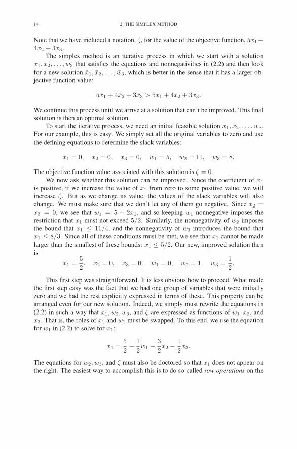
14 2. THE SIMPLEX METHOD
Note that we have included a notation, ζ, for the value of the objective function, 5x1 +4x2 + 3x3.
The simplex method is an iterative process in which we start with a solution
x1, x2, . . . , w3 that satisfies the equations and nonnegativities in (2.2) and then look
for a new solution x1, x2, . . . , w3, which is better in the sense that it has a larger ob-
jective function value:
5x1 + 4x2 + 3x3 > 5x1 + 4x2 + 3x3.
We continue this process until we arrive at a solution that can’t be improved. This final
solution is then an optimal solution.
To start the iterative process, we need an initial feasible solution x1, x2, . . . , w3.
For our example, this is easy. We simply set all the original variables to zero and use
the defining equations to determine the slack variables:
x1 = 0, x2 = 0, x3 = 0, w1 = 5, w2 = 11, w3 = 8.
The objective function value associated with this solution is ζ = 0.
We now ask whether this solution can be improved. Since the coefficient of x1
is positive, if we increase the value of x1 from zero to some positive value, we will
increase ζ. But as we change its value, the values of the slack variables will also
change. We must make sure that we don’t let any of them go negative. Since x2 =x3 = 0, we see that w1 = 5 − 2x1, and so keeping w1 nonnegative imposes the
restriction that x1 must not exceed 5/2. Similarly, the nonnegativity of w2 imposes
the bound that x1 ≤ 11/4, and the nonnegativity of w3 introduces the bound that
x1 ≤ 8/3. Since all of these conditions must be met, we see that x1 cannot be made
larger than the smallest of these bounds: x1 ≤ 5/2. Our new, improved solution then
is
x1 =5
2, x2 = 0, x3 = 0, w1 = 0, w2 = 1, w3 =
1
2.
This first step was straightforward. It is less obvious how to proceed. What made
the first step easy was the fact that we had one group of variables that were initially
zero and we had the rest explicitly expressed in terms of these. This property can be
arranged even for our new solution. Indeed, we simply must rewrite the equations in
(2.2) in such a way that x1, w2, w3, and ζ are expressed as functions of w1, x2, and
x3. That is, the roles of x1 and w1 must be swapped. To this end, we use the equation
for w1 in (2.2) to solve for x1:
x1 =5
2− 1
2w1 −
3
2x2 −
1
2x3.
The equations for w2, w3, and ζ must also be doctored so that x1 does not appear on
the right. The easiest way to accomplish this is to do so-called row operations on the

1. AN EXAMPLE 15
equations in (2.2). For example, if we take the equation for w2 and subtract two times
the equation for w1 and then bring the w1 term to the right-hand side, we get
w2 = 1 + 2w1 + 5x2.
Performing analogous row operations for w3 and ζ, we can rewrite the equations in
(2.2) as
(2.3)
ζ = 12.5− 2.5w1 − 3.5x2 + 0.5x3
x1 = 2.5− 0.5w1 − 1.5x2 − 0.5x3
w2 = 1 + 2w1 + 5x2
w3 = 0.5 + 1.5w1 + 0.5x2 − 0.5x3.
Note that we can recover our current solution by setting the “independent” variables
to zero and using the equations to read off the values for the “dependent” variables.
Now we see that increasing w1 or x2 will bring about a decrease in the objective
function value, and so x3, being the only variable with a positive coefficient, is the
only independent variable that we can increase to obtain a further increase in the ob-
jective function. Again, we need to determine how much this variable can be increased
without violating the requirement that all the dependent variables remain nonnegative.
This time we see that the equation for w2 is not affected by changes in x3, but the
equations for x1 and w3 do impose bounds, namely x3 ≤ 5 and x3 ≤ 1, respectively.
The latter is the tighter bound, and so the new solution is
x1 = 2, x2 = 0, x3 = 1, w1 = 0, w2 = 1, w3 = 0.
The corresponding objective function value is ζ = 13.
Once again, we must determine whether it is possible to increase the objective
function further and, if so, how. Therefore, we need to write our equations with
ζ, x1, w2, and x3 written as functions of w1, x2, and w3. Solving the last equation
in (2.3) for x3, we get
x3 = 1 + 3w1 + x2 − 2w3.
Also, performing the appropriate row operations, we can eliminate x3 from the other
equations. The result of these operations is
(2.4)
ζ = 13− w1 − 3x2 − w3
x1 = 2− 2w1 − 2x2 + w3
w2 = 1 + 2w1 + 5x2
x3 = 1 + 3w1 + x2 − 2w3.

16 2. THE SIMPLEX METHOD
We are now ready to begin the third iteration. The first step is to identify an
independent variable for which an increase in its value would produce a corresponding
increase in ζ. But this time there is no such variable, since all the variables have
negative coefficients in the expression for ζ. This fact not only brings the simplex
method to a standstill but also proves that the current solution is optimal. The reason
is quite simple. Since the equations in (2.4) are completely equivalent to those in
(2.2) and, since all the variables must be nonnegative, it follows that ζ ≤ 13 for every
feasible solution. Since our current solution attains the value of 13, we see that it is
indeed optimal.
1.1. Dictionaries, Bases, Etc. The systems of equations (2.2), (2.3), and (2.4)
that we have encountered along the way are called dictionaries. With the exception of
ζ, the variables that appear on the left (i.e., the variables that we have been referring
to as the dependent variables) are called basic variables. Those on the right (i.e., the
independent variables) are called nonbasic variables. The solutions we have obtained
by setting the nonbasic variables to zero are called basic feasible solutions.
2. The Simplex Method
Consider the general linear programming problem presented in standard form:
maximize
n∑
j=1
cjxj
subject to
n∑
j=1
aijxj ≤ bi i = 1, 2, . . . ,m
xj ≥ 0 j = 1, 2, . . . , n.
Our first task is to introduce slack variables and a name for the objective function
value:
(2.5)
ζ =n
∑
j=1
cjxj
wi = bi −n
∑
j=1
aijxj i = 1, 2, . . . , m.
As we saw in our example, as the simplex method proceeds, the slack variables be-
come intertwined with the original variables, and the whole collection is treated the
same. Therefore, it is at times convenient to have a notation in which the slack vari-
ables are more or less indistinguishable from the original variables. So we simply add
them to the end of the list of x-variables:
(x1, . . . , xn, w1, . . . , wm) = (x1, . . . , xn, xn+1, . . . , xn+m).

2. THE SIMPLEX METHOD 17
That is, we let xn+i = wi. With this notation, we can rewrite (2.5) as
ζ =n
∑
j=1
cjxj
xn+i = bi −n
∑
j=1
aijxj i = 1, 2, . . . ,m.
This is the starting dictionary. As the simplex method progresses, it moves from one
dictionary to another in its search for an optimal solution. Each dictionary has mbasic variables and n nonbasic variables. Let B denote the collection of indices from
{1, 2, . . . , n + m} corresponding to the basic variables, and let N denote the indices
corresponding to the nonbasic variables. Initially, we have N = {1, 2, . . . , n} and
B = {n + 1, n + 2, . . . , n + m}, but this of course changes after the first iteration.
Down the road, the current dictionary will look like this:
(2.6)
ζ = ζ +∑
j∈Ncjxj
xi = bi −∑
j∈Naijxj i ∈ B.
Note that we have put bars over the coefficients to indicate that they change as the
algorithm progresses.
Within each iteration of the simplex method, exactly one variable goes from non-
basic to basic and exactly one variable goes from basic to nonbasic. We saw this
process in our example, but let us now describe it in general.
The variable that goes from nonbasic to basic is called the entering variable. It
is chosen with the aim of increasing ζ; that is, one whose coefficient is positive: pick
k from {j ∈ N : cj > 0}. Note that if this set is empty, then the current solution is
optimal. If the set consists of more than one element (as is normally the case), then we
have a choice of which element to pick. There are several possible selection criteria,
some of which will be discussed in the next chapter. For now, suffice it to say that we
usually pick an index k having the largest coefficient (which again could leave us with
a choice).
The variable that goes from basic to nonbasic is called the leaving variable. It is
chosen to preserve nonnegativity of the current basic variables. Once we have decided
that xk will be the entering variable, its value will be increased from zero to a positive
value. This increase will change the values of the basic variables:
xi = bi − aikxk, i ∈ B.

18 2. THE SIMPLEX METHOD
We must ensure that each of these variables remains nonnegative. Hence, we require
that
(2.7) bi − aikxk ≥ 0, i ∈ B.
Of these expressions, the only ones that can go negative as xk increases are those for
which aik is positive; the rest remain fixed or increase. Hence, we can restrict our
attention to those i’s for which aik is positive. And for such an i, the value of xk at
which the expression becomes zero is
xk = bi/aik.
Since we don’t want any of these to go negative, we must raise xk only to the smallest
of all of these values:
xk = mini∈B:aik>0
bi/aik.
Therefore, with a certain amount of latitude remaining, the rule for selecting the leav-
ing variable is pick l from {i ∈ B : aik > 0 and bi/aik is minimal}.
The rule just given for selecting a leaving variable describes exactly the process
by which we use the rule in practice. That is, we look only at those variables for
which aik is positive and among those we select one with the smallest value of the
ratio bi/aik. There is, however, another, entirely equivalent, way to write this rule
which we will often use. To derive this alternate expression we use the convention
that 0/0 = 0 and rewrite inequalities (2.7) as
1
xk≥ aik
bi, i ∈ B
(we shall discuss shortly what happens when one of these ratios is an indeterminate
form 0/0 as well as what it means if none of the ratios are positive). Since we wish to
take the largest possible increase in xk, we see that
xk =
(
maxi∈B
aik
bi
)−1
.
Hence, the rule for selecting the leaving variable is as follows: pick l from {i ∈ B :aik/bi is maximal}.
The main difference between these two ways of writing the rule is that in one we
minimize the ratio of aik to bi whereas in the other we maximize the reciprocal ratio.
Of course, in the minimize formulation one must take care about the sign of the aik’s.
In the remainder of this book we will encounter these types of ratios often. We will
always write them in the maximize form since that is shorter to write, acknowledging
full well the fact that it is often more convenient, in practice, to do it the other way.

3. INITIALIZATION 19
Once the leaving-basic and entering-nonbasic variables have been selected, the
move from the current dictionary to the new dictionary involves appropriate row oper-
ations to achieve the interchange. This step from one dictionary to the next is called a
pivot.
As mentioned above, there is often more than one choice for the entering and the
leaving variables. Particular rules that make the choice unambiguous are called pivot
rules.
3. Initialization
In the previous section, we presented the simplex method. However, we only
considered problems for which the right-hand sides were all nonnegative. This ensured
that the initial dictionary was feasible. In this section, we shall discuss what one needs
to do when this is not the case.
Given a linear programming problem
maximize
n∑
j=1
cjxj
subject to
n∑
j=1
aijxj ≤ bi i = 1, 2, . . . ,m
xj ≥ 0 j = 1, 2, . . . , n,
the initial dictionary that we introduced in the preceding section was
ζ =
n∑
j=1
cjxj
wi = bi −n
∑
j=1
aijxj i = 1, 2, . . . , m.
The solution associated with this dictionary is obtained by setting each xj to zero and
setting each wi equal to the corresponding bi. This solution is feasible if and only
if all the right-hand sides are nonnegative. But what if they are not? We handle this
difficulty by introducing an auxiliary problem for which
(1) a feasible dictionary is easy to find and
(2) the optimal dictionary provides a feasible dictionary for the original prob-
lem.

20 2. THE SIMPLEX METHOD
The auxiliary problem is
maximize −x0
subject to
n∑
j=1
aijxj − x0 ≤ bi i = 1, 2, . . . ,m
xj ≥ 0 j = 0, 1, . . . , n.
It is easy to give a feasible solution to this auxiliary problem. Indeed, we simply set
xj = 0, for j = 1, . . . , n, and then pick x0 sufficiently large. It is also easy to see that
the original problem has a feasible solution if and only if the auxiliary problem has
a feasible solution with x0 = 0. In other words, the original problem has a feasible
solution if and only if the optimal solution to the auxiliary problem has objective value
zero.
Even though the auxiliary problem clearly has feasible solutions, we have not yet
shown that it has an easily obtained feasible dictionary. It is best to illustrate how to
obtain a feasible dictionary with an example:
maximize −2x1 − x2
subject to −x1 + x2 ≤−1
−x1 − 2x2 ≤−2
x2 ≤ 1
x1, x2 ≥ 0.
The auxiliary problem is
maximize −x0
subject to −x1 + x2 − x0 ≤−1
−x1 − 2x2 − x0 ≤−2
x2 − x0 ≤ 1
x0, x1, x2 ≥ 0.
Next we introduce slack variables and write down an initial infeasible dictionary:
ξ = − x0
w1 =−1 + x1 − x2 + x0
w2 =−2 + x1 + 2x2 + x0
w3 = 1 − x2 + x0.
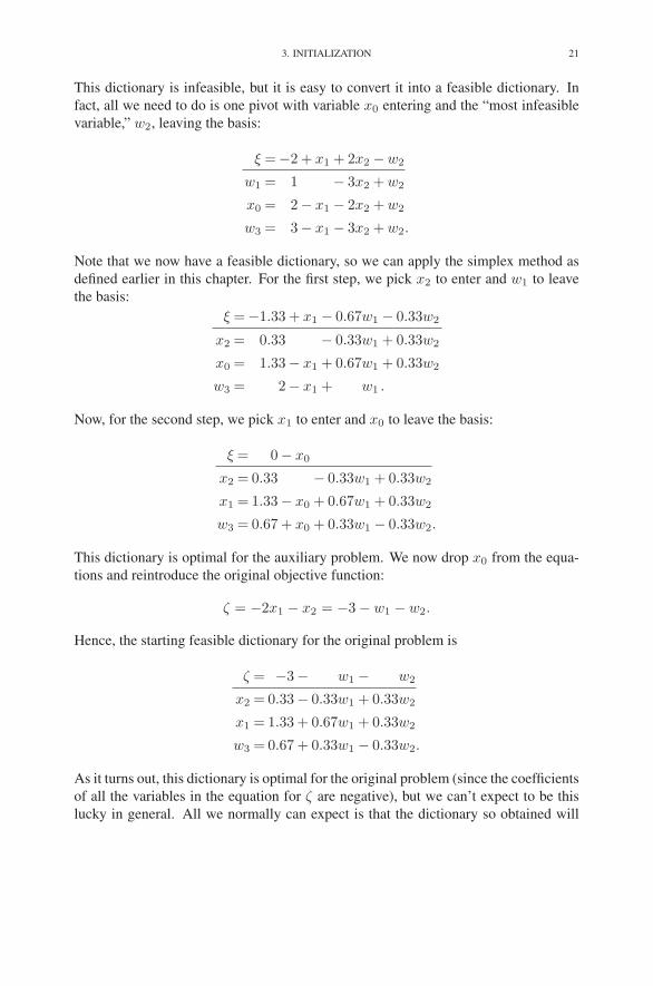
3. INITIALIZATION 21
This dictionary is infeasible, but it is easy to convert it into a feasible dictionary. In
fact, all we need to do is one pivot with variable x0 entering and the “most infeasible
variable,” w2, leaving the basis:
ξ =−2 + x1 + 2x2 −w2
w1 = 1 − 3x2 + w2
x0 = 2− x1 − 2x2 + w2
w3 = 3− x1 − 3x2 + w2.
Note that we now have a feasible dictionary, so we can apply the simplex method as
defined earlier in this chapter. For the first step, we pick x2 to enter and w1 to leave
the basis:
ξ =−1.33 + x1 − 0.67w1 − 0.33w2
x2 = 0.33 − 0.33w1 + 0.33w2
x0 = 1.33− x1 + 0.67w1 + 0.33w2
w3 = 2− x1 + w1 .
Now, for the second step, we pick x1 to enter and x0 to leave the basis:
ξ = 0− x0
x2 = 0.33 − 0.33w1 + 0.33w2
x1 = 1.33− x0 + 0.67w1 + 0.33w2
w3 = 0.67 + x0 + 0.33w1 − 0.33w2.
This dictionary is optimal for the auxiliary problem. We now drop x0 from the equa-
tions and reintroduce the original objective function:
ζ = −2x1 − x2 = −3 − w1 − w2.
Hence, the starting feasible dictionary for the original problem is
ζ = −3− w1 − w2
x2 = 0.33− 0.33w1 + 0.33w2
x1 = 1.33 + 0.67w1 + 0.33w2
w3 = 0.67 + 0.33w1 − 0.33w2.
As it turns out, this dictionary is optimal for the original problem (since the coefficients
of all the variables in the equation for ζ are negative), but we can’t expect to be this
lucky in general. All we normally can expect is that the dictionary so obtained will

22 2. THE SIMPLEX METHOD
be feasible for the original problem, at which point we continue to apply the simplex
method until an optimal solution is reached.
The process of solving the auxiliary problem to find an initial feasible solution is
often referred to as Phase I, whereas the process of going from a feasible solution to
an optimal solution is called Phase II.
4. Unboundedness
In this section, we shall discuss how to detect when the objective function value
is unbounded.
Let us now take a closer look at the “leaving variable” computation: pick l from
{i ∈ B : aik/bi is maximal}. We avoided the issue before, but now we must face what
to do if a denominator in one of these ratios vanishes. If the numerator is nonzero, then
it is easy to see that the ratio should be interpreted as plus or minus infinity depending
on the sign of the numerator. For the case of 0/0, the correct convention (as we’ll see
momentarily) is to take this as a zero.
What if all of the ratios, aik/bi, are nonpositive? In that case, none of the basic
variables will become zero as the entering variable increases. Hence, the entering
variable can be increased indefinitely to produce an arbitrarily large objective value.
In such situations, we say that the problem is unbounded. For example, consider the
following dictionary:
ζ = 5 + x3 − x1
x2 = 5 + 2x3 − 3x1
x4 = 7 − 4x1
x5 = x1.
The entering variable is x3 and the ratios are
−2/5, −0/7, 0/0.
Since none of these ratios is positive, the problem is unbounded.
In the next chapter, we will investigate what happens when some of these ratios
take the value +∞.
5. Geometry
When the number of variables in a linear programming problem is three or less,
we can graph the set of feasible solutions together with the level sets of the objective
function. From this picture, it is usually a trivial matter to write down the optimal
5. GEOMETRY 23
1 2 3 4 5 60
0
1
2
3
4
5
6
x1
x2
−x1+3x2=12x1+x2=8
2x1−x2=10
3x1+2x2=22
3x1+2x2=11
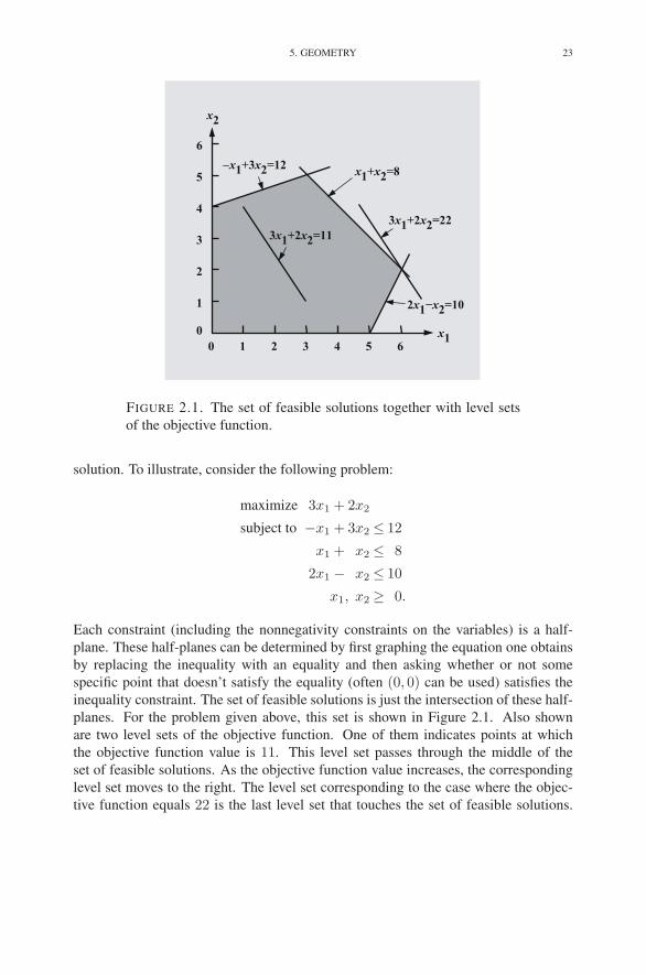
FIGURE 2.1. The set of feasible solutions together with level sets
of the objective function.
solution. To illustrate, consider the following problem:
maximize 3x1 + 2x2
subject to −x1 + 3x2 ≤ 12
x1 + x2 ≤ 8
2x1 − x2 ≤ 10
x1, x2 ≥ 0.
Each constraint (including the nonnegativity constraints on the variables) is a half-
plane. These half-planes can be determined by first graphing the equation one obtains
by replacing the inequality with an equality and then asking whether or not some
specific point that doesn’t satisfy the equality (often (0, 0) can be used) satisfies the
inequality constraint. The set of feasible solutions is just the intersection of these half-
planes. For the problem given above, this set is shown in Figure 2.1. Also shown
are two level sets of the objective function. One of them indicates points at which
the objective function value is 11. This level set passes through the middle of the
set of feasible solutions. As the objective function value increases, the corresponding
level set moves to the right. The level set corresponding to the case where the objec-
tive function equals 22 is the last level set that touches the set of feasible solutions.

24 2. THE SIMPLEX METHOD
Clearly, this is the maximum value of the objective function. The optimal solution is
the intersection of this level set with the set of feasible solutions. Hence, we see from
Figure 2.1 that the optimal solution is (x1, x2) = (6, 2).
Exercises
Solve the following linear programming problems. If you wish, you may check
your arithmetic by using the simple online pivot tool:
campuscgi.princeton.edu/∼rvdb/JAVA/pivot/simple.html
2.1 maximize 6x1 + 8x2 + 5x3 + 9x4
subject to 2x1 + x2 + x3 + 3x4 ≤ 5
x1 + 3x2 + x3 + 2x4 ≤ 3
x1, x2, x3, x4 ≥ 0.
2.2 maximize 2x1 + x2
subject to 2x1 + x2 ≤ 4
2x1 + 3x2 ≤ 3
4x1 + x2 ≤ 5
x1 + 5x2 ≤ 1
x1, x2 ≥ 0.
2.3 maximize 2x1 − 6x2
subject to −x1 − x2 − x3 ≤−2
2x1 − x2 + x3 ≤ 1
x1, x2, x3 ≥ 0.
2.4 maximize −x1 − 3x2 − x3
subject to 2x1 − 5x2 + x3 ≤−5
2x1 − x2 + 2x3 ≤ 4
x1, x2, x3 ≥ 0.
2.5 maximize x1 + 3x2
subject to −x1 − x2 ≤−3
−x1 + x2 ≤−1
x1 + 2x2 ≤ 4
x1, x2 ≥ 0.

EXERCISES 25
2.6 maximize x1 + 3x2
subject to −x1 − x2 ≤−3
−x1 + x2 ≤−1
x1 + 2x2 ≤ 2
x1, x2 ≥ 0.
2.7 maximize x1 + 3x2
subject to −x1 − x2 ≤−3
−x1 + x2 ≤−1
−x1 + 2x2 ≤ 2
x1, x2 ≥ 0.
2.8 maximize 3x1 + 2x2
subject to x1 − 2x2 ≤ 1
x1 − x2 ≤ 2
2x1 − x2 ≤ 6
x1 ≤ 5
2x1 + x2 ≤ 16
x1 + x2 ≤ 12
x1 + 2x2 ≤ 21
x2 ≤ 10
x1, x2 ≥ 0.
2.9 maximize 2x1 + 3x2 + 4x3
subject to − 2x2 − 3x3 ≥−5
x1 + x2 + 2x3 ≤ 4
x1 + 2x2 + 3x3 ≤ 7
x1, x2, x3 ≥ 0.
2.10 maximize 6x1 + 8x2 + 5x3 + 9x4
subject to x1 + x2 + x3 + x4 = 1
x1, x2, x3, x4 ≥ 0.
26 2. THE SIMPLEX METHOD
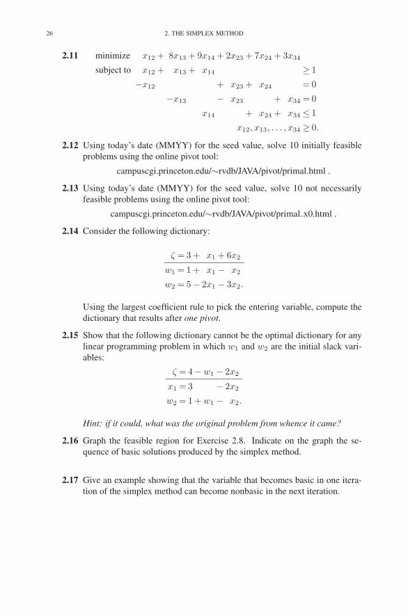
2.11 minimize x12 + 8x13 + 9x14 + 2x23 + 7x24 + 3x34
subject to x12 + x13 + x14 ≥ 1
−x12 + x23 + x24 = 0
−x13 − x23 + x34 = 0
x14 + x24 + x34 ≤ 1
x12, x13, . . . , x34 ≥ 0.
2.12 Using today’s date (MMYY) for the seed value, solve 10 initially feasible
problems using the online pivot tool:
campuscgi.princeton.edu/∼rvdb/JAVA/pivot/primal.html .
2.13 Using today’s date (MMYY) for the seed value, solve 10 not necessarily
feasible problems using the online pivot tool:
campuscgi.princeton.edu/∼rvdb/JAVA/pivot/primal x0.html .
2.14 Consider the following dictionary:
ζ = 3 + x1 + 6x2
w1 = 1 + x1 − x2
w2 = 5− 2x1 − 3x2.
Using the largest coefficient rule to pick the entering variable, compute the
dictionary that results after one pivot.
2.15 Show that the following dictionary cannot be the optimal dictionary for any
linear programming problem in which w1 and w2 are the initial slack vari-
ables:
ζ = 4−w1 − 2x2
x1 = 3 − 2x2
w2 = 1 + w1 − x2.
Hint: if it could, what was the original problem from whence it came?
2.16 Graph the feasible region for Exercise 2.8. Indicate on the graph the se-
quence of basic solutions produced by the simplex method.
2.17 Give an example showing that the variable that becomes basic in one itera-
tion of the simplex method can become nonbasic in the next iteration.

NOTES 27
2.18 Show that the variable that becomes nonbasic in one iteration of the simplex
method cannot become basic in the next iteration.
2.19 Solve the following linear programming problem:
maximize
n∑
j=1
pjxj
subject to
n∑
j=1
qjxj ≤ β
xj ≤ 1 j = 1, 2, . . . , n
xj ≥ 0 j = 1, 2, . . . , n.
Here, the numbers pj , j = 1, 2, . . . , n, are positive and sum to one. The
same is true of the qj’s:
n∑
j=1
qj = 1
qj > 0.
Furthermore (with only minor loss of generality), you may assume that
p1
q1<
p2
q2< · · · <
pn
qn.
Finally, the parameter β is a small positive number. See Exercise 1.3 for the
motivation for this problem.
Notes
The simplex method was invented by G.B. Dantzig in 1949. His monograph
(Dantzig 1963) is the classical reference. Most texts describe the simplex method as
a sequence of pivots on a table of numbers called the simplex tableau. Following
Chvatal (1983), we have developed the algorithm using the more memorable dictio-
nary notation.

CHAPTER 3
Degeneracy
In the previous chapter, we discussed what it means when the ratios computed to
calculate the leaving variable are all nonpositive (the problem is unbounded). In this
chapter, we take up the more delicate issue of what happens when some of the ratios
are infinite (i.e., their denominators vanish).
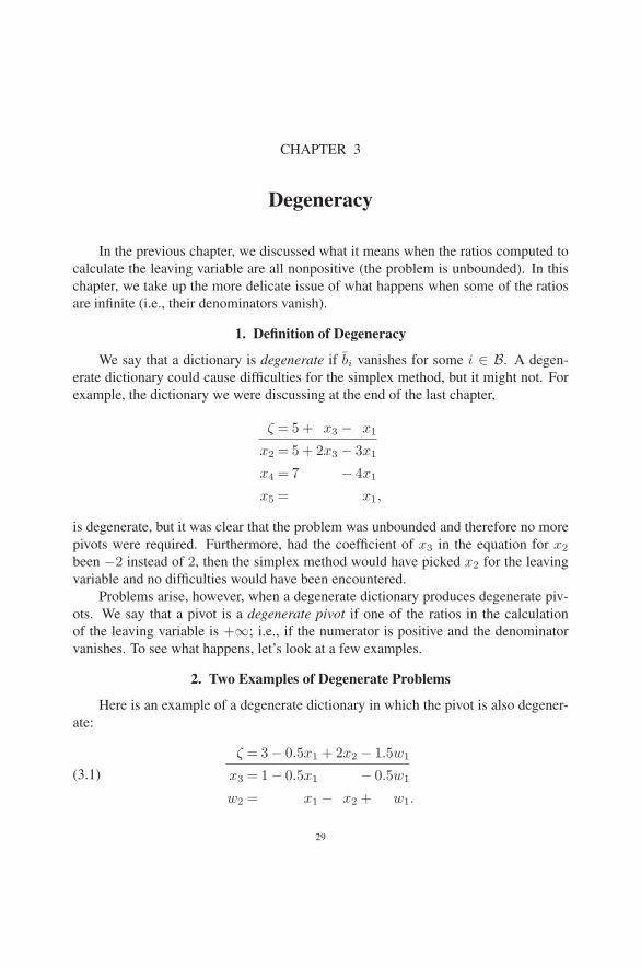
1. Definition of Degeneracy
We say that a dictionary is degenerate if bi vanishes for some i ∈ B. A degen-
erate dictionary could cause difficulties for the simplex method, but it might not. For
example, the dictionary we were discussing at the end of the last chapter,
ζ = 5 + x3 − x1
x2 = 5 + 2x3 − 3x1
x4 = 7 − 4x1
x5 = x1,
is degenerate, but it was clear that the problem was unbounded and therefore no more
pivots were required. Furthermore, had the coefficient of x3 in the equation for x2
been −2 instead of 2, then the simplex method would have picked x2 for the leaving
variable and no difficulties would have been encountered.
Problems arise, however, when a degenerate dictionary produces degenerate piv-
ots. We say that a pivot is a degenerate pivot if one of the ratios in the calculation
of the leaving variable is +∞; i.e., if the numerator is positive and the denominator
vanishes. To see what happens, let’s look at a few examples.
2. Two Examples of Degenerate Problems
Here is an example of a degenerate dictionary in which the pivot is also degener-
ate:
(3.1)
ζ = 3− 0.5x1 + 2x2 − 1.5w1
x3 = 1− 0.5x1 − 0.5w1
w2 = x1 − x2 + w1.
29
30 3. DEGENERACY
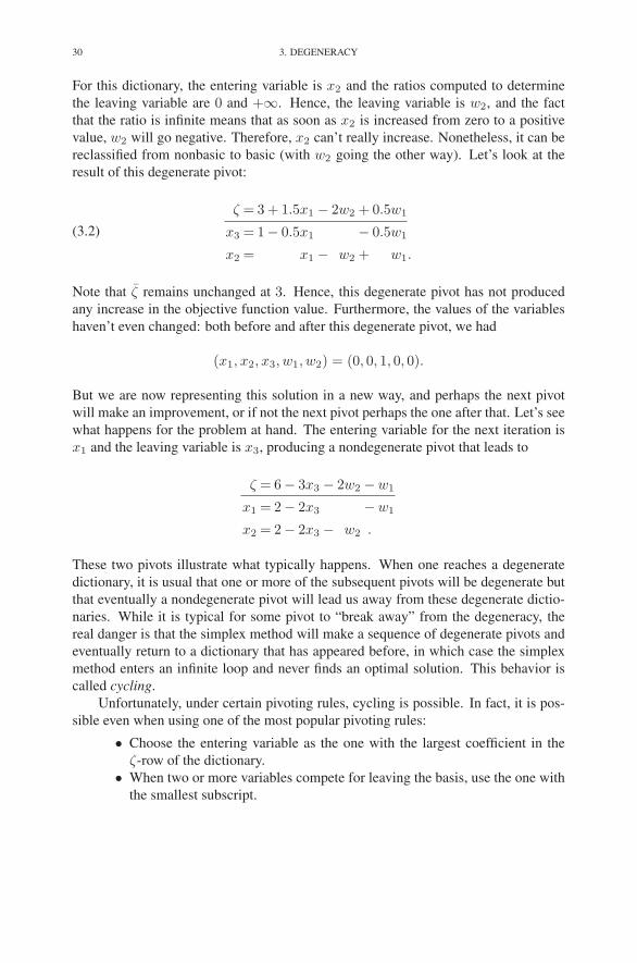
For this dictionary, the entering variable is x2 and the ratios computed to determine
the leaving variable are 0 and +∞. Hence, the leaving variable is w2, and the fact
that the ratio is infinite means that as soon as x2 is increased from zero to a positive
value, w2 will go negative. Therefore, x2 can’t really increase. Nonetheless, it can be
reclassified from nonbasic to basic (with w2 going the other way). Let’s look at the
result of this degenerate pivot:
(3.2)
ζ = 3 + 1.5x1 − 2w2 + 0.5w1
x3 = 1− 0.5x1 − 0.5w1
x2 = x1 − w2 + w1.
Note that ζ remains unchanged at 3. Hence, this degenerate pivot has not produced
any increase in the objective function value. Furthermore, the values of the variables
haven’t even changed: both before and after this degenerate pivot, we had
(x1, x2, x3, w1, w2) = (0, 0, 1, 0, 0).
But we are now representing this solution in a new way, and perhaps the next pivot
will make an improvement, or if not the next pivot perhaps the one after that. Let’s see
what happens for the problem at hand. The entering variable for the next iteration is
x1 and the leaving variable is x3, producing a nondegenerate pivot that leads to
ζ = 6− 3x3 − 2w2 −w1
x1 = 2− 2x3 −w1
x2 = 2− 2x3 − w2 .
These two pivots illustrate what typically happens. When one reaches a degenerate
dictionary, it is usual that one or more of the subsequent pivots will be degenerate but
that eventually a nondegenerate pivot will lead us away from these degenerate dictio-
naries. While it is typical for some pivot to “break away” from the degeneracy, the
real danger is that the simplex method will make a sequence of degenerate pivots and
eventually return to a dictionary that has appeared before, in which case the simplex
method enters an infinite loop and never finds an optimal solution. This behavior is
called cycling.
Unfortunately, under certain pivoting rules, cycling is possible. In fact, it is pos-
sible even when using one of the most popular pivoting rules:
• Choose the entering variable as the one with the largest coefficient in the
ζ-row of the dictionary.
• When two or more variables compete for leaving the basis, use the one with
the smallest subscript.
2. TWO EXAMPLES OF DEGENERATE PROBLEMS 31
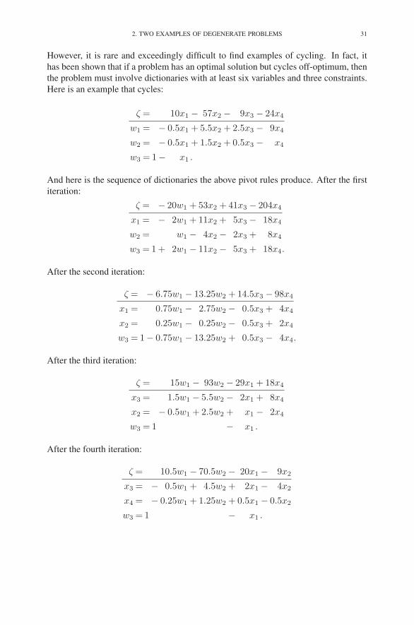
However, it is rare and exceedingly difficult to find examples of cycling. In fact, it
has been shown that if a problem has an optimal solution but cycles off-optimum, then
the problem must involve dictionaries with at least six variables and three constraints.
Here is an example that cycles:
ζ = 10x1 − 57x2 − 9x3 − 24x4
w1 = − 0.5x1 + 5.5x2 + 2.5x3 − 9x4
w2 = − 0.5x1 + 1.5x2 + 0.5x3 − x4
w3 = 1− x1 .
And here is the sequence of dictionaries the above pivot rules produce. After the first
iteration:
ζ = − 20w1 + 53x2 + 41x3 − 204x4
x1 = − 2w1 + 11x2 + 5x3 − 18x4
w2 = w1 − 4x2 − 2x3 + 8x4
w3 = 1 + 2w1 − 11x2 − 5x3 + 18x4.
After the second iteration:
ζ = − 6.75w1 − 13.25w2 + 14.5x3 − 98x4
x1 = 0.75w1 − 2.75w2 − 0.5x3 + 4x4
x2 = 0.25w1 − 0.25w2 − 0.5x3 + 2x4
w3 = 1− 0.75w1 − 13.25w2 + 0.5x3 − 4x4.
After the third iteration:
ζ = 15w1 − 93w2 − 29x1 + 18x4
x3 = 1.5w1 − 5.5w2 − 2x1 + 8x4
x2 = − 0.5w1 + 2.5w2 + x1 − 2x4
w3 = 1 − x1 .
After the fourth iteration:
ζ = 10.5w1 − 70.5w2 − 20x1 − 9x2
x3 = − 0.5w1 + 4.5w2 + 2x1 − 4x2
x4 = − 0.25w1 + 1.25w2 + 0.5x1 − 0.5x2
w3 = 1 − x1 .
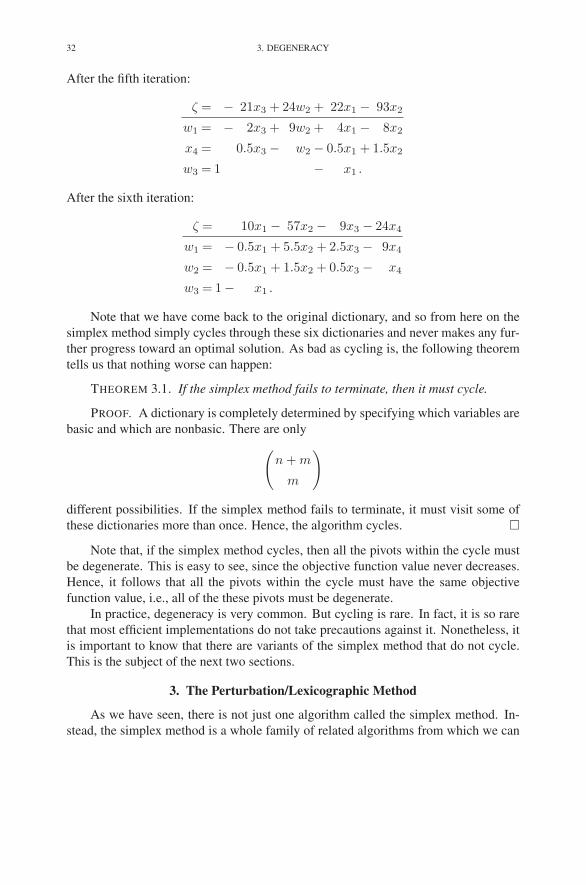
32 3. DEGENERACY
After the fifth iteration:
ζ = − 21x3 + 24w2 + 22x1 − 93x2
w1 = − 2x3 + 9w2 + 4x1 − 8x2
x4 = 0.5x3 − w2 − 0.5x1 + 1.5x2
w3 = 1 − x1 .
After the sixth iteration:
ζ = 10x1 − 57x2 − 9x3 − 24x4
w1 = − 0.5x1 + 5.5x2 + 2.5x3 − 9x4
w2 = − 0.5x1 + 1.5x2 + 0.5x3 − x4
w3 = 1− x1 .
Note that we have come back to the original dictionary, and so from here on the
simplex method simply cycles through these six dictionaries and never makes any fur-
ther progress toward an optimal solution. As bad as cycling is, the following theorem
tells us that nothing worse can happen:
THEOREM 3.1. If the simplex method fails to terminate, then it must cycle.
PROOF. A dictionary is completely determined by specifying which variables are
basic and which are nonbasic. There are only
(
n + m
m
)
different possibilities. If the simplex method fails to terminate, it must visit some of
these dictionaries more than once. Hence, the algorithm cycles. �
Note that, if the simplex method cycles, then all the pivots within the cycle must
be degenerate. This is easy to see, since the objective function value never decreases.
Hence, it follows that all the pivots within the cycle must have the same objective
function value, i.e., all of the these pivots must be degenerate.
In practice, degeneracy is very common. But cycling is rare. In fact, it is so rare
that most efficient implementations do not take precautions against it. Nonetheless, it
is important to know that there are variants of the simplex method that do not cycle.
This is the subject of the next two sections.
3. The Perturbation/Lexicographic Method
As we have seen, there is not just one algorithm called the simplex method. In-
stead, the simplex method is a whole family of related algorithms from which we can
3. THE PERTURBATION/LEXICOGRAPHIC METHOD 33
pick a specific instance by specifying what we have been referring to as pivoting rules.
We have also seen that, using the most natural pivoting rules, the simplex method can
fail to converge to an optimal solution by occasionally cycling indefinitely through a
sequence of degenerate pivots associated with a nonoptimal solution.
So this raises a natural question: are there pivoting rules for which the simplex
method will definitely either reach an optimal solution or prove that no such solution
exists? The answer to this question is yes, and we shall present two choices of such
pivoting rules.
The first method is based on the observation that degeneracy is sort of an accident.
That is, a dictionary is degenerate if one or more of the bi’s vanish. Our examples have
generally used small integers for the data, and in this case it doesn’t seem too surpris-
ing that sometimes cancellations occur and we end up with a degenerate dictionary.
But each right-hand side could in fact be any real number, and in the world of real
numbers the occurrence of any specific number, such as zero, seems to be quite un-
likely. So how about perturbing a given problem by adding small random perturbations
independently to each of the right-hand sides? If these perturbations are small enough,
we can think of them as insignificant and hence not really changing the problem. If
they are chosen independently, then the probability of an exact cancellation is zero.
Such random perturbation schemes are used in some implementations, but what
we have in mind as we discuss perturbation methods is something a little bit different.
Instead of using independent identically distributed random perturbations, let us con-
sider using a fixed perturbation for each constraint, with the perturbation getting much
smaller on each succeeding constraint. Indeed, we introduce a small positive number
ǫ1 for the first constraint and then a much smaller positive number ǫ2 for the second
constraint, etc. We write this as
0 < ǫm ≪ · · · ≪ ǫ2 ≪ ǫ1 ≪ all other data.
The idea is that each ǫi acts on an entirely different scale from all the other ǫi’s and
the data for the problem. What we mean by this is that no linear combination of the
ǫi’s using coefficients that might arise in the course of the simplex method can ever
produce a number whose size is of the same order as the data in the problem. Sim-
ilarly, each of the “lower down” ǫi’s can never “escalate” to a higher level. Hence,
cancellations can only occur on a given scale. Of course, this complete isolation of
scales can never be truly achieved in the real numbers, so instead of actually introduc-
ing specific values for the ǫi’s, we simply treat them as abstract symbols having these
scale properties.
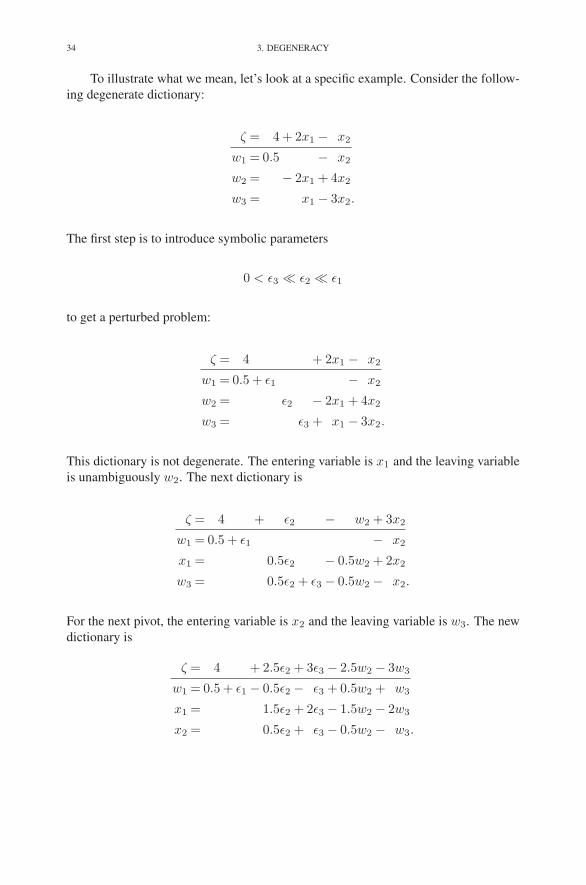
34 3. DEGENERACY
To illustrate what we mean, let’s look at a specific example. Consider the follow-
ing degenerate dictionary:
ζ = 4 + 2x1 − x2
w1 = 0.5 − x2
w2 = − 2x1 + 4x2
w3 = x1 − 3x2.
The first step is to introduce symbolic parameters
0 < ǫ3 ≪ ǫ2 ≪ ǫ1
to get a perturbed problem:
ζ = 4 + 2x1 − x2
w1 = 0.5 + ǫ1 − x2
w2 = ǫ2 − 2x1 + 4x2
w3 = ǫ3 + x1 − 3x2.
This dictionary is not degenerate. The entering variable is x1 and the leaving variable
is unambiguously w2. The next dictionary is
ζ = 4 + ǫ2 − w2 + 3x2
w1 = 0.5 + ǫ1 − x2
x1 = 0.5ǫ2 − 0.5w2 + 2x2
w3 = 0.5ǫ2 + ǫ3 − 0.5w2 − x2.
For the next pivot, the entering variable is x2 and the leaving variable is w3. The new
dictionary is
ζ = 4 + 2.5ǫ2 + 3ǫ3 − 2.5w2 − 3w3
w1 = 0.5 + ǫ1 − 0.5ǫ2 − ǫ3 + 0.5w2 + w3
x1 = 1.5ǫ2 + 2ǫ3 − 1.5w2 − 2w3
x2 = 0.5ǫ2 + ǫ3 − 0.5w2 − w3.

3. THE PERTURBATION/LEXICOGRAPHIC METHOD 35
This last dictionary is optimal. At this point, we simply drop the symbolic ǫi parame-
ters and get an optimal dictionary for the unperturbed problem:
ζ = 4− 2.5w2 − 3w3
w1 = 0.5 + 0.5w2 + w3
x1 = − 1.5w2 − 2w3
x2 = − 0.5w2 − w3.
When treating the ǫi’s as symbols, the method is called the lexicographic method.
Note that the lexicographic method does not affect the choice of entering variable but
does amount to a precise prescription for the choice of leaving variable.
It turns out that the lexicographic method produces a variant of the simplex method
that never cycles:
THEOREM 3.2. The simplex method always terminates provided that the leaving
variable is selected by the lexicographic rule.
PROOF. It suffices to show that no degenerate dictionary is ever produced. As
we’ve discussed before, the ǫi’s operate on different scales and hence can’t cancel
with each other. Therefore, we can think of the ǫi’s as a collection of independent
variables. Extracting the ǫ terms from the first dictionary, we see that we start with the
following pattern:
ǫ1
ǫ2. . .
ǫm.
And, after several pivots, the ǫ terms will form a system of linear combinations, say,
r11ǫ1 + r12ǫ2 . . . + r1mǫm
r21ǫ1 + r22ǫ2 . . . + r2mǫm
......
. . ....
rm1ǫ1 + rm2ǫ2 . . . + rmmǫm.
Since this system of linear combinations is obtained from the original system by pivot
operations and, since pivot operations are reversible, it follows that the rank of the
two systems must be the same. Since the original system had rank m, we see that
every subsequent system must have rank m. This means that there must be at least
one nonzero rij in every row i, which of course implies that none of the rows can be
degenerate. Hence, no dictionary can be degenerate. �

36 3. DEGENERACY
4. Bland’s Rule
The second pivoting rule we shall consider is called Bland’s rule. It stipulates
that both the entering and the leaving variable be selected from their respective sets of
choices by choosing the variable xk with the smallest index k.
THEOREM 3.3. The simplex method always terminates provided that both the
entering and the leaving variable are chosen according to Bland’s rule.
The proof may look rather involved, but the reader who spends the time to under-
stand it will find the underlying elegance most rewarding.
PROOF. It suffices to show that such a variant of the simplex method never cycles.
We prove this by assuming that cycling does occur and then showing that this assump-
tion leads to a contradiction. So let’s assume that cycling does occur. Without loss of
generality, we may assume that it happens from the beginning. Let D0, D1, . . . , Dk−1
denote the dictionaries through which the method cycles. That is, the simplex method
produces the following sequence of dictionaries:
D0, D1, . . . , Dk−1, D0, D1, . . . .
We say that a variable is fickle if it is in some basis and not in some other basis.
Let xt be the fickle variable having the largest index and let D denote a dictionary
in D0, D1, . . . , Dk−1 in which xt leaves the basis. Again, without loss of generality
we may assume that D = D0. Let xs denote the corresponding entering variable.
Suppose that D is recorded as follows:
ζ = v +∑
j∈Ncjxj
xi = bi −∑
j∈Naijxj i ∈ B.
Since xs is the entering variable and xt is the leaving variable, we have that s ∈ Nand t ∈ B.
Now let D∗ be a dictionary in D1, D2, . . . , Dk−1 in which xt enters the basis.
Suppose that D∗ is recorded as follows:
(3.3)
ζ = v∗ +∑
j∈N∗
c∗jxj
xi = b∗i −∑
j∈N∗
a∗ijxj i ∈ B∗.

4. BLAND’S RULE 37
Since all the dictionaries are degenerate, we have that v∗ = v, and therefore we can
write the objective function in (3.3) as
(3.4) ζ = v +
n+m∑
j=1
c∗jxj ,
where we have extended the notation c∗j to all variables (both original and slack) by
setting c∗j = 0 for j ∈ B∗.
Ignoring for the moment the possibility that some variables could go negative,
consider the solutions obtained by letting xs increase while holding all other variables
in N at zero:
xs = y,
xj = 0, j ∈ N \ {s},
xi = bi − aisy, i ∈ B.
The objective function at this point is given by
ζ = v + csy.
However, using (3.4), we see that it is also given by
ζ = v + c∗sy +∑
i∈Bc∗i (bi − aisy).
Equating these two expressions for ζ, we see that
(
cs − c∗s +∑
i∈Bc∗i ais
)
y =∑
i∈Bc∗i bi.
Since this equation must be an identity for every y, it follows that the coefficient
multiplying y must vanish (as must the right-hand side):
cs − c∗s +∑
i∈Bc∗i ais = 0.
Now, the fact that xs is the entering variable in D implies that
cs > 0.
38 3. DEGENERACY
Recall that xt is the fickle variable with the largest index. Since xs is also fickle, we
see that s < t. Since xs is not the entering variable in D∗ (as xt is), we see that
c∗s ≤ 0.
From these last three displayed equations, we get
∑
i∈Bc∗i ais < 0.
Hence, there must exist an index r ∈ B for which
(3.5) c∗rars < 0.
Consequently, c∗r �= 0 and r ∈ N ∗. Hence, xr is fickle and therefore r ≤ t. In fact,
r < t, since c∗t ats > 0. To see that this product is positive, note that both its factors
are positive: c∗t is positive, since xt is the entering variable in D∗, and ats is positive,
since xt is the leaving variable in D.
The fact that r < t implies that c∗r ≤ 0 (otherwise, according to the smallest index
criteria, r would be the entering variable for D∗). Hence, (3.5) implies that
ars > 0.
Now, since each of the dictionaries in the cycle describe the same solution, it follows
that every fickle variable is zero in all these dictionaries (since it is clearly zero in a
dictionary in which it is nonbasic). In particular, xr = 0. But in D, xr is basic. Hence,
br = 0.
These last two displayed equations imply that xr was a candidate to be the leaving
variable in D, and since r < t, it should have been chosen over xt. This is the
contradiction we have been looking for. �
5. Fundamental Theorem of Linear Programming
Now that we have a Phase I algorithm and a variant of the simplex method that
is guaranteed to terminate, we can summarize the main gist of this chapter in the
following theorem:
THEOREM 3.4. For an arbitrary linear program in standard form, the following
statements are true:
(1) If there is no optimal solution, then the problem is either infeasible or un-
bounded.
(2) If a feasible solution exists, then a basic feasible solution exists.
(3) If an optimal solution exists, then a basic optimal solution exists.

6. GEOMETRY 39
1 2x2
x3
x1
x1+2x3=3
x2+2x3=2x2=0
FIGURE 3.1. The set of feasible solutions for the problem given by (3.6).
PROOF. The Phase I algorithm either proves that the problem is infeasible or
produces a basic feasible solution. The Phase II algorithm either discovers that the
problem is unbounded or finds a basic optimal solution. These statements depend, of
course, on applying a variant of the simplex method that does not cycle, which we
now know to exist. �
6. Geometry
As we saw in the previous chapter, the set of feasible solutions for a problem in
two dimensions is the intersection of a number of halfplanes, i.e., a polygon. In three
dimensions, the situation is similar. Consider, for example, the following problem:
(3.6)
maximize x1 + 2x2 + 3x3
subject to x1 + 2x3 ≤ 3
x2 + 2x3 ≤ 2
x1, x2, x3 ≥ 0.

40 3. DEGENERACY
The set of points satisfying x1 + 2x3 = 3 is a plane. The inequality x1 + 2x3 ≤ 3therefore consists of all points on one side of this plane; that is, it is a halfspace.
The same is true for each of the other four inequalities. The feasible set consists of
those points in space that satisfy all five inequalities, i.e., those points lying in the
intersection of these halfspaces. This set is the polyhedron shown in Figure 3.1. This
polyhedron is bordered by five facets, each facet being a portion of one of the planes
that was defined by replacing a constraint inequality with an equation. For example,
the “front” facet in the figure is a portion of the plane x1+2x3 = 3. The facets acquire
a particularly simple description if we introduce slack variables into the problem:
w1 = 3− x1 − 2x3
w2 = 2 − x2 − 2x3.
Indeed, each facet corresponds precisely to some variable (either original or slack)
vanishing. For instance, the front facet in the figure corresponds to w1 = 0 whereas
the “left” facet corresponds to x2 = 0.
The correspondences can be continued. Indeed, each edge of the polyhedron cor-
responds to a pair of variables vanishing. For example, the edge lying at the interface
of the left and the front facets in the figure corresponds to both w1 = 0 and x2 = 0.
Going further yet, each vertex of the polyhedron corresponds to three variables
vanishing. For instance, the vertex whose coordinates are (1, 0, 1) corresponds to
w1 = 0, x2 = 0, and w2 = 0.
Now, let’s think about applying the simplex method to this problem. Every basic
feasible solution involves two basic variables and three nonbasic variables. Further-
more, the three nonbasic variables are, by definition, zero in the basic feasible solution.
Therefore, for this example, the basic feasible solutions stand in one-to-one correspon-
dence with the vertices of the polyhedron. In fact, applying the simplex method to this
problem, one discovers that the sequence of vertices visited by the algorithm is
(0, 0, 0) −→ (0, 0, 1) −→ (1, 0, 1) −→ (3, 2, 0).
The example we’ve been considering has the nice property that every vertex is
formed by the intersection of exactly three of the facets. But consider now the follow-
ing problem:
(3.7)
maximize x1 + 2x2 + 3x3
subject to x1 + 2x3 ≤ 2
x2 + 2x3 ≤ 2
x1, x2, x3 ≥ 0.
Algebraically, the only difference between this problem and the previous one is that
the right-hand side of the first inequality is now a 2 instead of a 3. But look at the
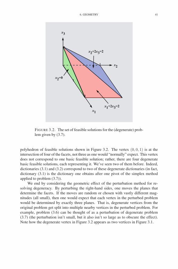
6. GEOMETRY 41
1
x2
x3
x1
x1+2x3=2
x2=0
x2+2x3=2
FIGURE 3.2. The set of feasible solutions for the (degenerate) prob-
lem given by (3.7).
polyhedron of feasible solutions shown in Figure 3.2. The vertex (0, 0, 1) is at the
intersection of four of the facets, not three as one would “normally” expect. This vertex
does not correspond to one basic feasible solution; rather, there are four degenerate
basic feasible solutions, each representing it. We’ve seen two of them before. Indeed,
dictionaries (3.1) and (3.2) correspond to two of these degenerate dictionaries (in fact,
dictionary (3.1) is the dictionary one obtains after one pivot of the simplex method
applied to problem (3.7)).
We end by considering the geometric effect of the perturbation method for re-
solving degeneracy. By perturbing the right-hand sides, one moves the planes that
determine the facets. If the moves are random or chosen with vastly different mag-
nitudes (all small), then one would expect that each vertex in the perturbed problem
would be determined by exactly three planes. That is, degenerate vertices from the
original problem get split into multiple nearby vertices in the perturbed problem. For
example, problem (3.6) can be thought of as a perturbation of degenerate problem
(3.7) (the perturbation isn’t small, but it also isn’t so large as to obscure the effect).
Note how the degenerate vertex in Figure 3.2 appears as two vertices in Figure 3.1.
42 3. DEGENERACY
Exercises
3.1 Solve the following linear program using the perturbation method to resolve
degeneracy:
maximize 10x1 − 57x2 − 9x3 − 24x4
subject to 0.5x1 − 5.5x2 − 2.5x3 + 9x4 ≤ 0
0.5x1 − 1.5x2 − 0.5x3 + x4 ≤ 0
x1 ≤ 1
x1, x2, x3, x4 ≥ 0.
Note: The simple pivot tool with the Lexicographic labels can be used to
check your arithmetic:
campuscgi.princeton.edu/∼rvdb/JAVA/pivot/simple.html
3.2 Solve the following linear program using Bland’s rule to resolve degeneracy:
maximize 10x1 − 57x2 − 9x3 − 24x4
subject to 0.5x1 − 5.5x2 − 2.5x3 + 9x4 ≤ 0
0.5x1 − 1.5x2 − 0.5x3 + x4 ≤ 0
x1 ≤ 1
x1, x2, x3, x4 ≥ 0.
3.3 Using today’s date (MMYY) for the seed value, solve 10 possibly degener-
ate problems using the online pivot tool:
campuscgi.princeton.edu/∼rvdb/JAVA/pivot/lexico.html .
3.4 Consider the linear programming problems whose right-hand sides are iden-
tically zero:
maximize
n∑
j=1
cjxj
subject to
n∑
j=1
aijxj ≤ 0 i = 1, 2, . . . ,m
xj ≥ 0 j = 1, 2, . . . , n.
Show that either xj = 0 for all j is optimal or else the problem is unbounded.
NOTES 43
3.5 Consider the following linear program:
maximize x1 + 3x2
subject to −2x1 ≤−5
x1 ≥ 0 .
Show that this problem has feasible solutions but no vertex solutions. How
does this reconcile with the fundamental theorem of linear programming
(Theorem 3.4)?
3.6 Suppose that a linear programming problem has the following property: its
initial dictionary is not degenerate and, when solved by the simplex method,
there is never a tie for the choice of leaving variable.
(a) Can such a problem have degenerate dictionaries? Explain.
(b) Can such a problem cycle? Explain.
3.7 Consider the following dictionary:
ζ = 5 + 2x2 − 2x3 + 3x5
x6 = 4− 2x2 − x3 + x5
x4 = 2− x2 + x3 − x5
x1 = 6− 2x2 − 2x3 − 3x5.
(a) List all pairs (xr, xs) such that xr could be the entering variable and xs
could be the leaving variable.
(b) List all such pairs if the largest-coefficient rule for choosing the entering
variable is used.
(c) List all such pairs if Bland’s rule for choosing the entering and leaving
variables is used.
Notes
The first example of cycling was given by Hoffman (1953). The fact that any
linear programming problem that cycles must have at least six variables and three
constraints was proved by Marshall & Suurballe (1969).
Early proofs of the fundamental theorem of linear programming (Theorem 3.4)
were constructive, relying, as in our development, on the existence of a variant of
the simplex method that works even in the presense of degeneracy. Hence, finding
such variants occupied the attention of early researchers in linear programming. The
perturbation method was first suggested by A. Orden and developed independently

44 3. DEGENERACY
by Charnes (1952). The essentially equivalent lexicographic method first appeared in
Dantzig et al. (1955). Theorem 3.3 was proved by Bland (1977).
For an extensive treatment of degeneracy issues see Gal (1993).
CHAPTER 4
Efficiency of the Simplex Method
In the previous chapter, we saw that the simplex method (with appropriate piv-
oting rules to guarantee no cycling) will solve any linear programming problem for
which an optimal solution exists. In this chapter, we investigate just how fast it will
solve a problem of a given size.
1. Performance Measures
Performance measures can be broadly divided into two types:
• worst case
• average case.
As its name implies, a worst-case analysis looks at all problems of a given “size” and
asks how much effort is needed to solve the hardest of these problems. Similarly,
an average-case analysis looks at the average amount of effort, averaging over all
problems of a given size. Worst-case analyses are generally easier than average-case
analyses. The reason is that, for worst-case analyses, one simply needs to give an
upper bound on how much effort is required and then exhibit a specific example that
attains this bound. However, for average-case analyses, one must have a stochastic
model of the space of “random linear programming problems” and then be able to
say something about the solution effort averaged over all the problems in the sample
space. There are two serious difficulties here. The first is that it is not clear at all how
one should model the space of random problems. Secondly, given such a model, one
must be able to evaluate the amount of effort required to solve every problem in the
sample space.
Therefore, worst-case analysis is more tractable than average-case analysis, but it
is also less relevant to a person who needs to solve real problems. In this chapter, we
shall give a worst-case analysis of the simplex method. Later, in Chapter 12, we shall
present results of empirical studies that indicate the average behavior over finite sets
of real problems. Such studies act as a surrogate for a true average-case analysis.
2. Measuring the Size of a Problem
Before looking at worst cases, we must discuss two issues. First, how do we
specify the size of a problem? Two parameters come naturally to mind: m and n.
45
46 4. EFFICIENCY OF THE SIMPLEX METHOD
Usually, we shall simply use these two numbers to characterize the size a problem.
However, we should mention some drawbacks associated with this choice. First of
all, it would be preferable to use only one number to indicate size. Since the data
for a problem consist of the constraint coefficients together with the right-hand side
and objective function coefficients, perhaps we should use the total number of data
elements, which is roughly mn.
The product mn isn’t bad, but what if many or even most of the data elements are
zero? Wouldn’t one expect such a problem to be easier to solve? Efficient implemen-
tations do indeed take advantage of the presence of lots of zeros, and so an analysis
should also account for this. Hence, a good measure might be simply the number
of nonzero data elements. This would definitely be an improvement, but one can go
further. On a computer, floating-point numbers are all the same size and can be mul-
tiplied in the same amount of time. But if a person is to solve a problem by hand (or
use unlimited precision computation on a computer), then certainly multiplying 23 by
7 is a lot easier than multiplying 23453.2352 by 86833.245643. So perhaps the best
measure of a problem’s size is not the number of data elements, but the actual number
of bits needed to store all the data on a computer. This measure is popular among most
computer scientists and is usually denoted by L.
However, with a little further abstraction, the size of the data, L, is seen to be
ambiguous. As we saw in Chapter 1, real-world problems, while generally large and
sparse, usually can be described quite simply and involve only a small amount of true
input data that gets greatly expanded when setting the problem up with a constraint
matrix, right-hand side, and objective function. So should L represent the number of
bits needed to specify the nonzero constraint coefficients, objective coefficients, and
right-hand sides, or should it be the number of bits in the original data set plus the
number of bits in the description of how this data represents a linear programming
problem? No one currently uses this last notion of problem size, but it seems fairly
reasonable that they should (or at least that they should seriously consider it). Anyway,
our purpose here is merely to mention that these important issues are lurking about,
but, as stated above, we shall simply focus on m and n to characterize the size of a
problem.
3. Measuring the Effort to Solve a Problem
The second issue to discuss is how one should measure the amount of work re-
quired to solve a problem. The best answer is the number of seconds of computer
time required to solve the problem, using the computer sitting on one’s desk. Un-
fortunately, there are (hopefully) many readers of this text, not all of whom use the
exact same computer. Even if they did, computer technology changes rapidly, and
a few years down the road everyone would be using something entirely different. It
would be nice if the National Institute of Standards and Technology (the government
organization in charge of setting standards, such as how many threads/inch a standard

4. WORST-CASE ANALYSIS OF THE SIMPLEX METHOD 47
light bulb should have) would identify a standard computer for the purpose of bench-
marking algorithms, but, needless to say, this is not very likely. So the time needed to
solve a problem, while the most desirable measure, is not the most practical one here.
Fortunately, there is a fairly reasonable substitute. Algorithms are generally iterative
processes, and the time to solve a problem can be factored into the number of iterations
required to solve the problem times the amount of time required to do each iteration.
The first factor, the number of iterations, does not depend on the computer and so
is a reasonable surrogate for the actual time. This surrogate is useful when compar-
ing various algorithms within the same general class of algorithms, in which the time
per iteration can be expected to be about the same among the algorithms; however, it
becomes meaningless when one wishes to compare two entirely different algorithms.
For now, we shall measure the amount of effort to solve a linear programming problem
by counting the number of iterations needed to solve it.
4. Worst-Case Analysis of the Simplex Method
How bad can the simplex method be in the worst case? Well, we have already
seen that for some pivoting rules it can cycle, and hence the worst-case solution time
for such variants is infinite. However, what about noncycling variants of the simplex
method? Since the simplex method operates by moving from one basic feasible solu-
tion to another without ever returning to a previously visited solution, an upper bound
on the number of iterations is simply the number of basic feasible solutions, of which
there can be at most
(
n + m
m
)
.
For a fixed value of the sum n + m, this expression is maximized when m = n. And
how big is it? It is not hard to show that
1
2n22n ≤
(
2n
n
)
≤ 22n
(see Exercise 4.9). It should be noted that, even though typographically compact, the
expression 2n is huge even when n is not very big. For example, 250 = 1.1259×10¹⁵.
Our best chance for finding a bad example is to look at the case where m = n.
We shall now give an example, first discovered by V. Klee and G.J. Minty in 1972, in
which the simplex method using the largest coefficient rule requires 2n − 1 iterations
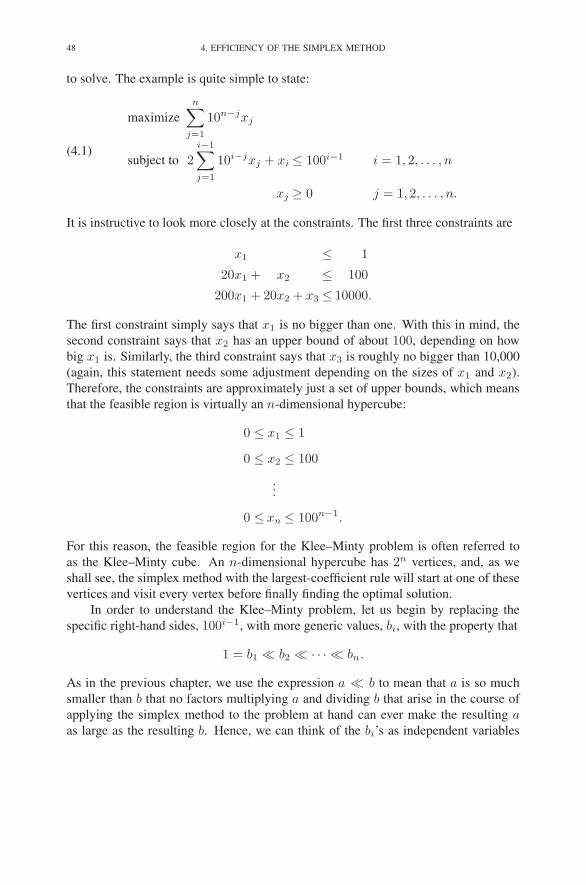
48 4. EFFICIENCY OF THE SIMPLEX METHOD
to solve. The example is quite simple to state:
(4.1)
maximize
n∑
j=1
10n−jxj
subject to 2i−1∑
j=1
10i−jxj + xi ≤ 100i−1 i = 1, 2, . . . , n
xj ≥ 0 j = 1, 2, . . . , n.
It is instructive to look more closely at the constraints. The first three constraints are
x1 ≤ 1
20x1 + x2 ≤ 100
200x1 + 20x2 + x3 ≤ 10000.
The first constraint simply says that x1 is no bigger than one. With this in mind, the
second constraint says that x2 has an upper bound of about 100, depending on how
big x1 is. Similarly, the third constraint says that x3 is roughly no bigger than 10,000
(again, this statement needs some adjustment depending on the sizes of x1 and x2).
Therefore, the constraints are approximately just a set of upper bounds, which means
that the feasible region is virtually an n-dimensional hypercube:
0 ≤ x1 ≤ 1
0 ≤ x2 ≤ 100
...
0 ≤ xn ≤ 100n−1.
For this reason, the feasible region for the Klee–Minty problem is often referred to
as the Klee–Minty cube. An n-dimensional hypercube has 2n vertices, and, as we
shall see, the simplex method with the largest-coefficient rule will start at one of these
vertices and visit every vertex before finally finding the optimal solution.
In order to understand the Klee–Minty problem, let us begin by replacing the
specific right-hand sides, 100i−1, with more generic values, bi, with the property that
1 = b1 ≪ b2 ≪ · · · ≪ bn.
As in the previous chapter, we use the expression a ≪ b to mean that a is so much
smaller than b that no factors multiplying a and dividing b that arise in the course of
applying the simplex method to the problem at hand can ever make the resulting aas large as the resulting b. Hence, we can think of the bi’s as independent variables
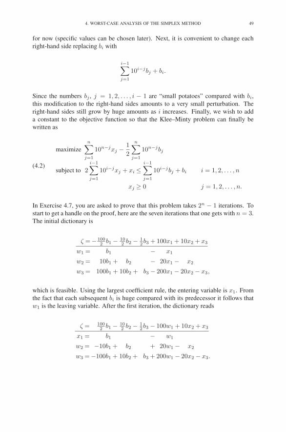
4. WORST-CASE ANALYSIS OF THE SIMPLEX METHOD 49
for now (specific values can be chosen later). Next, it is convenient to change each
right-hand side replacing bi with
i−1∑
j=1
10i−jbj + bi.
Since the numbers bj , j = 1, 2, . . . , i − 1 are “small potatoes” compared with bi,
this modification to the right-hand sides amounts to a very small perturbation. The
right-hand sides still grow by huge amounts as i increases. Finally, we wish to add
a constant to the objective function so that the Klee–Minty problem can finally be
written as
(4.2)
maximize
n∑
j=1
10n−jxj −1
2
n∑
j=1
10n−jbj
subject to 2
i−1∑
j=1
10i−jxj + xi ≤i−1∑
j=1
10i−jbj + bi i = 1, 2, . . . , n
xj ≥ 0 j = 1, 2, . . . , n.
In Exercise 4.7, you are asked to prove that this problem takes 2n − 1 iterations. To
start to get a handle on the proof, here are the seven iterations that one gets with n = 3.
The initial dictionary is
ζ =− 1002 b1 − 10
2 b2 − 12b3 + 100x1 + 10x2 + x3
w1 = b1 − x1
w2 = 10b1 + b2 − 20x1 − x2
w3 = 100b1 + 10b2 + b3 − 200x1 − 20x2 − x3,
which is feasible. Using the largest coefficient rule, the entering variable is x1. From
the fact that each subsequent bi is huge compared with its predecessor it follows that
w1 is the leaving variable. After the first iteration, the dictionary reads
ζ = 1002 b1 − 10
2 b2 − 12b3 − 100w1 + 10x2 + x3
x1 = b1 − w1
w2 = −10b1 + b2 + 20w1 − x2
w3 =−100b1 + 10b2 + b3 + 200w1 − 20x2 − x3.

50 4. EFFICIENCY OF THE SIMPLEX METHOD
Now, x2 enters and w2 leaves, so after the second iteration we get:
ζ =− 1002 b1 + 10
2 b2 − 12b3 + 100w1 − 10w2 + x3
x1 = b1 − w1
x2 = −10b1 + b2 + 20w1 − w2
w3 = 100b1 − 10b2 + b3 − 200w1 + 20w2 − x3.
After the third iteration
ζ = 1002 b1 + 10
2 b2 − 12b3 − 100x1 − 10w2 + x3
w1 = b1 − x1
x2 = 10b1 + b2 − 20x1 − w2
w3 =−100b1 − 10b2 + b3 + 200x1 + 20w2 − x3.
After the fourth iteration
ζ = − 1002 b1 − 10
2 b2 + 12b3 + 100x1 + 10w2 −w3
w1 = b1 − x1
x2 = 10b1 + b2 − 20x1 − w2
x3 =−100b1 − 10b2 + b3 + 200x1 + 20w2 −w3.
After the fifth iteration
ζ = 1002 b1 − 10
2 b2 + 12b3 − 100w1 + 10w2 −w3
x1 = b1 − w1
x2 =−10b1 + b2 + 20w1 − w2
x3 = 100b1 − 10b2 + b3 − 200w1 + 20w2 −w3.
After the sixth iteration
ζ = − 1002 b1 + 10
2 b2 + 12b3 + 100w1 − 10x2 −w3
x1 = b1 − w1
w2 = −10b1 + b2 + 20w1 − x2
x3 =−100b1 + 10b2 + b3 + 200w1 − 20x2 −w3.

4. WORST-CASE ANALYSIS OF THE SIMPLEX METHOD 51
And, finally, after the seventh iteration, we get
ζ = 1002 b1 + 10
2 b2 + 12b3 − 100x1 − 10x2 −w3
w1 = b1 − x1
w2 = 10b1 + b2 − 20x1 − x2
x3 = 100b1 + 10b2 + b3 − 200x1 − 20x2 −w3,
which is, of course, optimal.
A few observations should be made. First, every pivot is the swap of an xj with
the corresponding wj . Second, every dictionary looks just like the first one with the
exception that the wi’s and the xi’s have become intertwined and various signs have
changed (see Exercise 4.6).
Also note that the final dictionary could have been reached from the initial dictio-
nary in just one pivot if we had selected x3 to be the entering variable. But the largest-
coefficient rule dictated selecting x1. It is natural to wonder whether the largest-
coefficient rule could be replaced by some other pivot rule for which the worst-case
behavior would be much better than the 2n behavior of the largest-coefficient rule. So
far no one has found such a pivot rule. However, no one has proved that such a rule
does not exist either.
Finally, we mention that one desirable property of an algorithm is that it be scale
invariant. This means that should the units in which one measures the decision vari-
ables in a problem be changed, the algorithm would still behave in exactly the same
manner. The simplex method with the largest-coefficient rule is not scale invariant. To
see this, consider changing variables in the Klee–Minty problem by putting
xj = 100j−1xj .
In the new variables, the initial dictionary for the n = 3 Klee–Minty problem becomes
ζ =− 1002 b1 − 10
2 b2 − 12b3 + 100x1 + 1000x2 + 10000x3
w1 = b1 − x1
w2 = 10b1 + b2 − 20x1 − x2
w3 = 100b1 + 1000b2 + b3 − 200x1 − 2000x2 − 10000x3.
Now, the largest-coefficient rule picks variable x3 to enter. Variable w3 leaves, and
the method steps to the optimal solution in just one iteration. There exist pivot rules
for the simplex method that are scale invariant. But Klee–Minty-like examples have
been found for most proposed alternative pivot rules (whether scale invariant or not).
In fact, it is an open question whether there exist pivot rules for which one can prove
that no problem instance requires an exponential number of iterations (as a function
of m or n).

52 4. EFFICIENCY OF THE SIMPLEX METHOD
Exercises
In solving the following problems, the simple pivot tool can be used to check your
arithmetic:
campuscgi.princeton.edu/∼rvdb/JAVA/pivot/simple.html
4.1 Compare the performance of the largest-coefficient and the smallest-index
pivoting rules on the following linear program:
maximize 4x1 + 5x2
subject to 2x1 + 2x2 ≤ 9
x1 ≤ 4
x2 ≤ 3
x1, x2 ≥ 0.
4.2 Compare the performance of the largest-coefficient and the smallest-index
pivoting rules on the following linear program:
maximize 2x1 + x2
subject to 3x1 + x2 ≤ 3
x1, x2 ≥ 0.
4.3 Compare the performance of the largest-coefficient and the smallest-index
pivoting rules on the following linear program:
maximize 3x1 + 5x2
subject to x1 + 2x2 ≤ 5
x1 ≤ 3
x2 ≤ 2
x1, x2 ≥ 0.
4.4 Solve the Klee–Minty problem (4.1) for n = 3.
4.5 Solve the 4 variable Klee-Minty problem using the online pivot tool:
campuscgi.princeton.edu/∼rvdb/JAVA/pivot/kleeminty.html
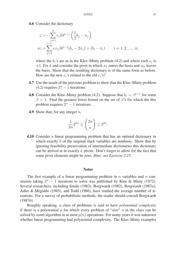
NOTES 53
4.6 Consider the dictionary
ζ =−n
∑
j=1
ǫj10n−j
(
1
2bj − xj
)
wi =
i−1∑
j=1
ǫiǫj10i−j(bj − 2xj) + (bi − xi) i = 1, 2, . . . , n,
where the bi’s are as in the Klee–Minty problem (4.2) and where each ǫi is
±1. Fix k and consider the pivot in which xk enters the basis and wk leaves
the basis. Show that the resulting dictionary is of the same form as before.
How are the new ǫi’s related to the old ǫi’s?
4.7 Use the result of the previous problem to show that the Klee–Minty problem
(4.2) requires 2n − 1 iterations.
4.8 Consider the Klee–Minty problem (4.2). Suppose that bi = βi−1 for some
β > 1. Find the greatest lower bound on the set of β’s for which the this
problem requires 2n − 1 iterations.
4.9 Show that, for any integer n,
1
2n22n ≤
(
2n
n
)
≤ 22n.
4.10 Consider a linear programming problem that has an optimal dictionary in
which exactly k of the original slack variables are nonbasic. Show that by
ignoring feasibility preservation of intermediate dictionaries this dictionary
can be arrived at in exactly k pivots. Don’t forget to allow for the fact that
some pivot elements might be zero. Hint: see Exercise 2.15.
Notes
The first example of a linear programming problem in n variables and n con-
straints taking 2n − 1 iterations to solve was published by Klee & Minty (1972).
Several researchers, including Smale (1983), Borgwardt (1982), Borgwardt (1987a),
Adler & Megiddo (1985), and Todd (1986), have studied the average number of it-
erations. For a survey of probabilistic methods, the reader should consult Borgwardt
(1987b).
Roughly speaking, a class of problems is said to have polynomial complexity
if there is a polynomial p for which every problem of “size” n in the class can be
solved by some algorithm in at most p(n) operations. For many years it was unknown
whether linear programming had polynomial complexity. The Klee–Minty examples

54 4. EFFICIENCY OF THE SIMPLEX METHOD
show that, if linear programming is polynomial, then the simplex method is not the
algorithm that gives the polynomial bound, since 2n is not dominated by any polyno-
mial. In 1979, Khachian (1979) gave a new algorithm for linear programming, called
the ellipsoid method, which is polynomial and therefore established once and for all
that linear programming has polynomial complexity. The collection of all problem
classes having polynomial complexity is usually denoted by P . A class of problems
is said to belong to the class NP if, given a (proposed) solution, one can verify its
optimality in a number of operations that is bounded by some polynomial in the “size”
of the problem. Clearly, P ⊂ NP (since, if we can solve from scratch in a polyno-
mial amount of time, surely we can verify optimality at least that fast). An important
problem in theoretical computer science is to determine whether or not P is a strict
subset of NP .
The study of how difficult it is to solve a class of problems is called complexity
theory. Readers interested in pursuing this subject further should consult Garey &
Johnson (1977).
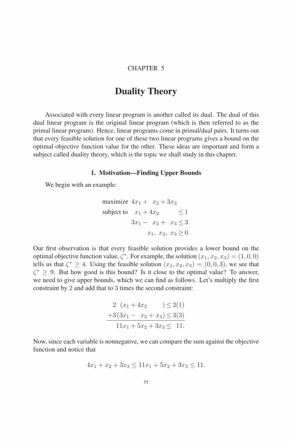
CHAPTER 5
Duality Theory
Associated with every linear program is another called its dual. The dual of this
dual linear program is the original linear program (which is then referred to as the
primal linear program). Hence, linear programs come in primal/dual pairs. It turns out
that every feasible solution for one of these two linear programs gives a bound on the
optimal objective function value for the other. These ideas are important and form a
subject called duality theory, which is the topic we shall study in this chapter.
1. Motivation—Finding Upper Bounds
We begin with an example:
maximize 4x1 + x2 + 3x3
subject to x1 + 4x2 ≤ 1
3x1 − x2 + x3 ≤ 3
x1, x2, x3 ≥ 0.
Our first observation is that every feasible solution provides a lower bound on the
optimal objective function value, ζ∗. For example, the solution (x1, x2, x3) = (1, 0, 0)tells us that ζ∗ ≥ 4. Using the feasible solution (x1, x2, x3) = (0, 0, 3), we see that
ζ∗ ≥ 9. But how good is this bound? Is it close to the optimal value? To answer,
we need to give upper bounds, which we can find as follows. Let’s multiply the first
constraint by 2 and add that to 3 times the second constraint:
2 (x1 + 4x2 )≤ 2(1)
+3(3x1 − x2 + x3)≤ 3(3)
11x1 + 5x2 + 3x3 ≤ 11.
Now, since each variable is nonnegative, we can compare the sum against the objective
function and notice that
4x1 + x2 + 3x3 ≤ 11x1 + 5x2 + 3x3 ≤ 11.
55

56 5. DUALITY THEORY
Hence, ζ∗ ≤ 11. We have localized the search to somewhere between 9 and 11. These
bounds leave a gap (within which the optimal solution lies), but they are better than
nothing. Furthermore, they can be improved. To get a better upper bound, we again
apply the same upper bounding technique, but we replace the specific numbers we
used before with variables and then try to find the values of those variables that give
us the best upper bound. So we start by multiplying the two constraints by nonnegative
numbers, y1 and y2, respectively. The fact that these numbers are nonnegative implies
that they preserve the direction of the inequalities. Hence,
y1( x1 + 4x2 )≤ y1
+y2(3x1 − x2 + x3)≤ 3y2
(y1 + 3y2)x1 + (4y1 − y2)x2 + (y2)x3 ≤ y1 + 3y2.
If we stipulate that each of the coefficients of the xi’s be at least as large as the corre-
sponding coefficient in the objective function,
y1 + 3y2 ≥ 4
4y1 − y2 ≥ 1
y2 ≥ 3,
then we can compare the objective function against this sum (and its bound):
ζ = 4x1 + x2 + 3x3
≤ (y1 + 3y2)x1 + (4y1 − y2)x2 + (y2)x3
≤ y1 + 3y2.
We now have an upper bound, y1 + 3y2, which we should minimize in our effort to
obtain the best possible upper bound. Therefore, we are naturally led to the following
optimization problem:
minimize y1 + 3y2
subject to y1 + 3y2 ≥ 4
4y1 − y2 ≥ 1
y2 ≥ 3
y1, y2 ≥ 0.
This problem is called the dual linear programming problem associated with the given
linear programming problem. In the next section, we will define the dual linear pro-
gramming problem in general.
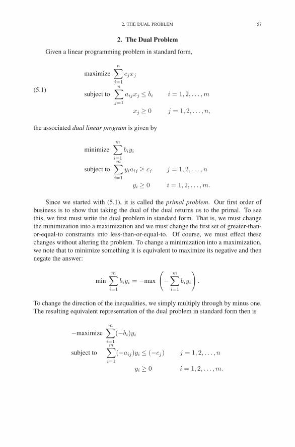
2. THE DUAL PROBLEM 57
2. The Dual Problem
Given a linear programming problem in standard form,
(5.1)
maximize
n∑
j=1
cjxj
subject to
n∑
j=1
aijxj ≤ bi i = 1, 2, . . . ,m
xj ≥ 0 j = 1, 2, . . . , n,
the associated dual linear program is given by
minimize
m∑
i=1
biyi
subject to
m∑
i=1
yiaij ≥ cj j = 1, 2, . . . , n
yi ≥ 0 i = 1, 2, . . . ,m.
Since we started with (5.1), it is called the primal problem. Our first order of
business is to show that taking the dual of the dual returns us to the primal. To see
this, we first must write the dual problem in standard form. That is, we must change
the minimization into a maximization and we must change the first set of greater-than-
or-equal-to constraints into less-than-or-equal-to. Of course, we must effect these
changes without altering the problem. To change a minimization into a maximization,
we note that to minimize something it is equivalent to maximize its negative and then
negate the answer:
min
m∑
i=1
biyi = −max
(
−m∑
i=1
biyi
)
.
To change the direction of the inequalities, we simply multiply through by minus one.
The resulting equivalent representation of the dual problem in standard form then is
−maximize
m∑
i=1
(−bi)yi
subject to
m∑
i=1
(−aij)yi ≤ (−cj) j = 1, 2, . . . , n
yi ≥ 0 i = 1, 2, . . . ,m.

58 5. DUALITY THEORY
Now we can take its dual:
−minimize
n∑
j=1
(−cj)xj
subject to
n∑
j=1
(−aij)xj ≥ (−bi) i = 1, 2, . . . ,m
xj ≥ 0 j = 1, 2, . . . , n,
which is clearly equivalent to the primal problem as formulated in (5.1).
3. The Weak Duality Theorem
As we saw in our example, the dual problem provides upper bounds for the primal
objective function value. This result is true in general and is referred to as the Weak
Duality Theorem:
THEOREM 5.1. If (x1, x2, . . . , xn) is feasible for the primal and (y1, y2, . . . , ym)is feasible for the dual, then
∑
j
cjxj ≤∑
i
biyi.
PROOF. The proof is a simple chain of obvious inequalities:
∑
j
cjxj ≤∑
j
(
∑
i
yiaij
)
xj
=∑
ij
yiaijxj
=∑
i
⎛
⎝
∑
j
aijxj
⎞
⎠ yi
≤∑
i
biyi,
where the first inequality follows from the fact that each xj is nonnegative and each
cj is no larger than∑
i yiaij . The second inequality, of course, holds for similar
reasons. �
Consider the subset of the real line consisting of all possible values for the primal
objective function, and consider the analogous subset associated with the dual prob-
lem. The weak duality theorem tells us that the set of primal values lies entirely to

3. THE WEAK DUALITY THEOREM 59
] [
Primal Values Dual Values
Gap
]
Primal Values Dual Values
No Gap
[
FIGURE 5.1. The primal objective values are all less than the dual
objective values. An important question is whether or not there is a
gap between the largest primal value and the smallest dual value.
the left of the set of dual values. As we shall see shortly, these sets are both closed
intervals (perhaps of infinite extent), and the right endpoint of the primal set butts up
against the left endpoint of the dual set (see Figure 5.1). That is, there is no gap be-
tween the optimal objective function value for the primal and for the dual. The lack
of a gap between primal and dual objective values provides a convenient tool for veri-
fying optimality. Indeed, if we can exhibit a feasible primal solution (x∗1, x
∗2, . . . , x
∗n)
and a feasible dual solution (y∗1 , y∗
2 , . . . , y∗m) for which
∑
j
cjx∗j =
∑
i
biy∗i ,
then we may conclude that each of these solutions is optimal for its respective prob-
lem. To see that the primal solution is optimal, consider any other feasible solution
(x1, x2, . . . , xn). By the weak duality theorem, we have that
∑
j
cjxj ≤∑
i
biy∗i =
∑
j
cjx∗j .
Now, since (x∗1, x
∗2, . . . , x
∗n) was assumed to be feasible, we see that it must be opti-
mal. An analogous argument shows that the dual solution is also optimal for the dual
problem. As an example, consider the solutions x = (0, 0.25, 3.25) and y = (1, 3) in
our example. Both these solutions are feasible, and both yield an objective value of
10. Hence, the weak duality theorem says that these solutions are optimal.
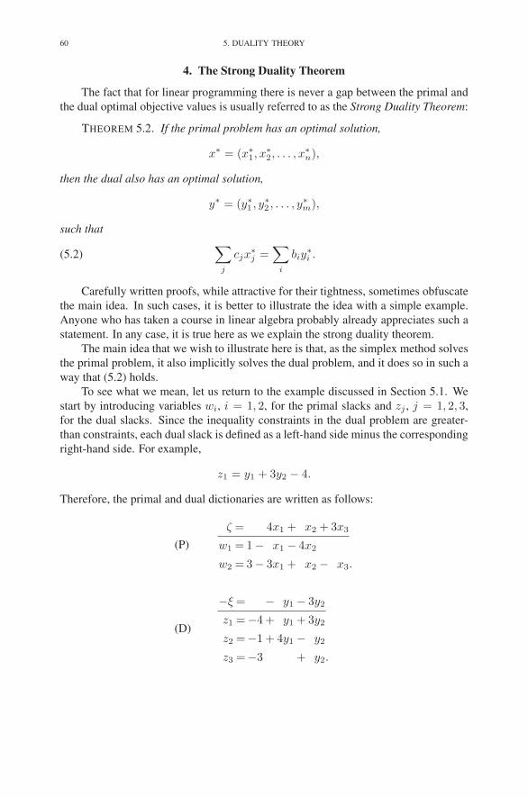
60 5. DUALITY THEORY
4. The Strong Duality Theorem
The fact that for linear programming there is never a gap between the primal and
the dual optimal objective values is usually referred to as the Strong Duality Theorem:
THEOREM 5.2. If the primal problem has an optimal solution,
x∗ = (x∗1, x
∗2, . . . , x
∗n),
then the dual also has an optimal solution,
y∗ = (y∗1 , y∗
2 , . . . , y∗m),
such that
(5.2)∑
j
cjx∗j =
∑
i
biy∗i .
Carefully written proofs, while attractive for their tightness, sometimes obfuscate
the main idea. In such cases, it is better to illustrate the idea with a simple example.
Anyone who has taken a course in linear algebra probably already appreciates such a
statement. In any case, it is true here as we explain the strong duality theorem.
The main idea that we wish to illustrate here is that, as the simplex method solves
the primal problem, it also implicitly solves the dual problem, and it does so in such a
way that (5.2) holds.
To see what we mean, let us return to the example discussed in Section 5.1. We
start by introducing variables wi, i = 1, 2, for the primal slacks and zj , j = 1, 2, 3,
for the dual slacks. Since the inequality constraints in the dual problem are greater-
than constraints, each dual slack is defined as a left-hand side minus the corresponding
right-hand side. For example,
z1 = y1 + 3y2 − 4.
Therefore, the primal and dual dictionaries are written as follows:
(P)
ζ = 4x1 + x2 + 3x3
w1 = 1− x1 − 4x2
w2 = 3− 3x1 + x2 − x3.
(D)
−ξ = − y1 − 3y2
z1 =−4 + y1 + 3y2
z2 =−1 + 4y1 − y2
z3 =−3 + y2.
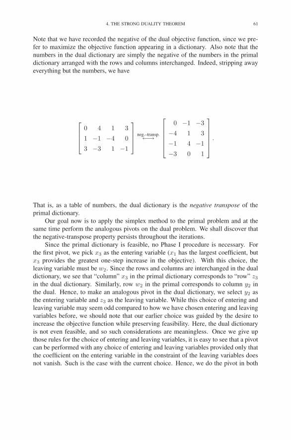
4. THE STRONG DUALITY THEOREM 61
Note that we have recorded the negative of the dual objective function, since we pre-
fer to maximize the objective function appearing in a dictionary. Also note that the
numbers in the dual dictionary are simply the negative of the numbers in the primal
dictionary arranged with the rows and columns interchanged. Indeed, stripping away
everything but the numbers, we have
⎡
⎢
⎢
⎣
0 4 1 3
1 −1 −4 0
3 −3 1 −1
⎤
⎥
⎥
⎦
neg.–transp.←→
⎡
⎢
⎢
⎢
⎢
⎣
0 −1 −3
−4 1 3
−1 4 −1
−3 0 1
⎤
⎥
⎥
⎥
⎥
⎦
.
That is, as a table of numbers, the dual dictionary is the negative transpose of the
primal dictionary.
Our goal now is to apply the simplex method to the primal problem and at the
same time perform the analogous pivots on the dual problem. We shall discover that
the negative-transpose property persists throughout the iterations.
Since the primal dictionary is feasible, no Phase I procedure is necessary. For
the first pivot, we pick x3 as the entering variable (x1 has the largest coefficient, but
x3 provides the greatest one-step increase in the objective). With this choice, the
leaving variable must be w2. Since the rows and columns are interchanged in the dual
dictionary, we see that “column” x3 in the primal dictionary corresponds to “row” z3
in the dual dictionary. Similarly, row w2 in the primal corresponds to column y2 in
the dual. Hence, to make an analogous pivot in the dual dictionary, we select y2 as
the entering variable and z3 as the leaving variable. While this choice of entering and
leaving variable may seem odd compared to how we have chosen entering and leaving
variables before, we should note that our earlier choice was guided by the desire to
increase the objective function while preserving feasibility. Here, the dual dictionary
is not even feasible, and so such considerations are meaningless. Once we give up
those rules for the choice of entering and leaving variables, it is easy to see that a pivot
can be performed with any choice of entering and leaving variables provided only that
the coefficient on the entering variable in the constraint of the leaving variables does
not vanish. Such is the case with the current choice. Hence, we do the pivot in both

62 5. DUALITY THEORY
the primal and the dual. The result is
(P)
ζ = 9− 5x1 + 4x2 − 3w2
w1 = 1− x1 − 4x2
x3 = 3− 3x1 + x2 − w2.
(D)
−ξ =−9− y1 − 3z3
z1 = 5 + y1 + 3z3
z2 =−4 + 4y1 − z3
y2 = 3 + z3.
Note that these two dictionaries still have the property of being negative-transposes
of each other. For the next pivot, the entering variable in the primal dictionary is x2
(this time there is no choice) and the leaving variable is w1. In the dual dictionary, the
corresponding entering variable is y1 and the leaving variable is z2. Doing the pivots,
we get
(P)
ζ = 10− 6x1 − w1 − 3w2
x2 = 0.25− 0.25x1 − 0.25w1
x3 = 3.25− 3.25x1 − 0.25w1 − w2.
(D)
−ξ =−10− 0.25z2 − 3.25z3
z1 = 6 + 0.25z2 + 3.25z3
y1 = 1 + 0.25z2 + 0.25z3
y2 = 3 + z3.
This primal dictionary is optimal, since the coefficients in the objective row are all
negative. Looking at the dual dictionary, we see that it is now feasible for the anal-
ogous reason. In fact, it is optimal too. Finally, both the primal and dual objective
function values are 10.
The situation should now be clear. Given a linear programming problem, which
is assumed to possess an optimal solution, first apply the Phase I procedure to get a
basic feasible starting dictionary for Phase II. Then apply the simplex method to find
an optimal solution. Each primal dictionary generated by the simplex method implic-
itly defines a corresponding dual dictionary as follows: first write down the negative
transpose and then replace each xj with a zj and each wi with a yi. As long as the pri-
mal dictionary is not optimal, the implicitly defined dual dictionary will be infeasible.
But once an optimal primal dictionary is found, the corresponding dual dictionary will
be feasible. Since its objective coefficients are always nonpositive, this feasible dual
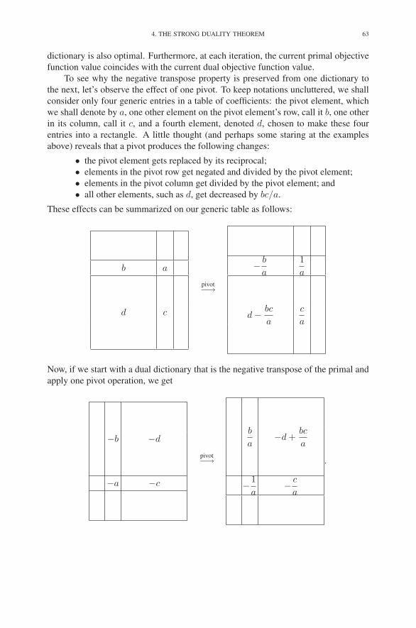
4. THE STRONG DUALITY THEOREM 63
dictionary is also optimal. Furthermore, at each iteration, the current primal objective
function value coincides with the current dual objective function value.
To see why the negative transpose property is preserved from one dictionary to
the next, let’s observe the effect of one pivot. To keep notations uncluttered, we shall
consider only four generic entries in a table of coefficients: the pivot element, which
we shall denote by a, one other element on the pivot element’s row, call it b, one other
in its column, call it c, and a fourth element, denoted d, chosen to make these four
entries into a rectangle. A little thought (and perhaps some staring at the examples
above) reveals that a pivot produces the following changes:
• the pivot element gets replaced by its reciprocal;
• elements in the pivot row get negated and divided by the pivot element;
• elements in the pivot column get divided by the pivot element; and
• all other elements, such as d, get decreased by bc/a.
These effects can be summarized on our generic table as follows:
b a
d c
pivot−→
− b
a
1
a
d − bc
a
c
a
Now, if we start with a dual dictionary that is the negative transpose of the primal and
apply one pivot operation, we get
−b −d
−a −c
pivot−→
b
a−d +
bc
a
−1
a− c
a
.

64 5. DUALITY THEORY
Note that the resulting dual table is the negative transpose of the resulting primal table.
By induction we then conclude that, if we start with this property, it will be preserved
throughout the solution process.
Since the strong duality theorem is the most important theorem in this book, we
present here a careful proof. Those readers who are satisfied with the above discussion
may skip the proof.
PROOF OF THEOREM 5.2. It suffices to exhibit a dual feasible solution y∗ satis-
fying (5.2). Suppose we apply the simplex method. We know that the simplex method
produces an optimal solution whenever one exists, and we have assumed that one does
indeed exist. Hence, the final dictionary will be an optimal dictionary for the primal
problem. The objective function in this final dictionary is ordinarily written as
ζ = ζ +∑
j∈Ncjxj .
But, since this is the optimal dictionary and we prefer stars to bars for denoting optimal
“stuff,” let us write ζ∗ instead of ζ. Also, the collection of nonbasic variables will
generally consist of a combination of original variables as well as slack variables.
Instead of using cj for the coefficients of these variables, let us use c∗j for the objective
coefficients corresponding to original variables, and let us use d∗i for the objective
coefficients corresponding to slack variables. Also, for those original variables that
are basic we put c∗j = 0, and for those slack variables that are basic we put d∗i = 0.
With these new notations, we can rewrite the objective function as
ζ = ζ∗ +
n∑
j=1
c∗jxj +
m∑
i=1
d∗i wi.
As we know, ζ∗ is the objective function value corresponding to the optimal primal
solution:
(5.3) ζ∗ =n
∑
j=1
cjx∗j .
Now, put
(5.4) y∗i = −d∗i , i = 1, 2, . . . ,m.

4. THE STRONG DUALITY THEOREM 65
We shall show that y∗ = (y∗1 , y∗
2 , . . . , y∗m) is feasible for the dual problem and satisfies
(5.2). To this end, we write the objective function two ways:
n∑
j=1
cjxj = ζ∗ +
n∑
j=1
c∗jxj +
m∑
i=1
d∗i wi
= ζ∗ +
n∑
j=1
c∗jxj +
m∑
i=1
(−y∗i )
⎛
⎝bi −n
∑
j=1
aijxj
⎞
⎠
= ζ∗ −m∑
i=1
biy∗i +
n∑
j=1
(
c∗j +m∑
i=1
y∗i aij
)
xj .
Since all these expressions are linear in the variables xj , we can equate the coefficients
of each variable appearing on the left-hand side with the corresponding coefficient
appearing in the last expression on the right-hand side. We can also equate the constant
terms on the two sides. Hence,
ζ∗ =m∑
i=1
biy∗i(5.5)
cj = c∗j +
m∑
i=1
y∗i aij , j = 1, 2, . . . , n.(5.6)
Combining (5.3) and (5.5), we get that (5.2) holds. Also, the optimality of the dic-
tionary for the primal problem implies that each c∗j is nonpositive, and hence we see
from (5.6) thatm∑
i=1
y∗i aij ≥ cj , j = 1, 2, . . . , n.
By the same reasoning, each d∗i is nonpositive, and so we see from (5.4) that
y∗i ≥ 0, i = 1, 2, . . . ,m.
These last two sets of inequalities are precisely the conditions that guarantee dual
feasibility. This completes the proof. �
The strong duality theorem tells us that, whenever the primal problem has an
optimal solution, the dual problem has one also and there is no duality gap. But what
if the primal problem does not have an optimal solution? For example, suppose that
it is unbounded. The unboundedness of the primal together with the weak duality
theorem tells us immediately that the dual problem must be infeasible. Similarly, if
the dual problem is unbounded, then the primal problem must be infeasible. It is
66 5. DUALITY THEORY
natural to hope that these three cases are the only possibilities, because if they were
we could then think of the strong duality theorem holding globally. That is, even if,
say, the primal is unbounded, the fact that then the dual is infeasible is like saying that
the primal and dual have a zero duality gap sitting out at +∞. Similarly, an infeasible
primal together with an unbounded dual could be viewed as a pair in which the gap is
zero and sits at −∞.
But it turns out that there is a fourth possibility that sometimes occurs—it can hap-
pen that both the primal and the dual problems are infeasible. For example, consider
the following problem:
maximize 2x1 − x2
subject to x1 − x2 ≤ 1
−x1 + x2 ≤−2
x1, x2 ≥ 0.
It is easy to see that both this problem and its dual are infeasible. For these problems,
one can think of there being a huge duality gap extending from −∞ to +∞.
Duality theory is often useful in that it provides a certificate of optimality. For
example, suppose that you were asked to solve a really huge and difficult linear pro-
gram. After spending weeks or months at the computer, you are finally able to get the
simplex method to solve the problem, producing as it does an optimal dual solution
y∗ in addition to the optimal primal solution x∗. Now, how are you going to convince
your boss that your solution is correct? Do you really want to ask her to verify the
correctness of your computer programs? The answer is probably not. And in fact it
is not necessary. All you need to do is supply the primal and the dual solution, and
she only has to check that the primal solution is feasible for the primal problem (that’s
easy), the dual solution is feasible for the dual problem (that’s just as easy), and the
primal and dual objective values agree (and that’s even easier). Certificates of optimal-
ity have also been known to dramatically reduce the amount of time certain underpaid
professors have to devote to grading homework assignments!
As we’ve seen, the simplex method applied to a primal problem actually solves
both the primal and the dual. Since the dual of the dual is the primal, applying the
simplex method to the dual also solves both the primal and the dual problem. Some-
times it is easier to apply the simplex method to the dual, for example, if the dual has
an obvious basic feasible solution but the primal does not. We take up this topic in the
next chapter.
5. Complementary Slackness
Sometimes it is necessary to recover an optimal dual solution when only an opti-
mal primal solution is known. The following theorem, known as the Complementary
Slackness Theorem, can help in this regard.

5. COMPLEMENTARY SLACKNESS 67
THEOREM 5.3. Suppose that x = (x1, x2, . . . , xn) is primal feasible and that
y = (y1, y2, . . . , ym) is dual feasible. Let (w1, w2, . . . , wm) denote the corresponding
primal slack variables, and let (z1, z2, . . . , zn) denote the corresponding dual slack
variables. Then x and y are optimal for their respective problems if and only if
xjzj = 0, for j = 1, 2, . . . , n,
wiyi = 0, for i = 1, 2, . . . ,m.(5.7)
PROOF. We begin by revisiting the chain of inequalities used to prove the weak
duality theorem:
∑
j
cjxj ≤∑
j
(
∑
i
yiaij
)
xj(5.8)
=∑
i
⎛
⎝
∑
j
aijxj
⎞
⎠ yi
≤∑
i
biyi.(5.9)
Recall that the first inequality arises from the fact that each term in the left-hand sum
is dominated by the corresponding term in the right-hand sum. Furthermore, this
domination is a consequence of the fact that each xj is nonnegative and
cj ≤∑
i
yiaij .
Hence, inequality (5.8) will be an equality if and only if, for every j = 1, 2, . . . , n,
either xj = 0 or cj =∑
i yiaij . But since
zj =∑
i
yiaij − cj ,
we see that the alternative to xj = 0 is simply that zj = 0. Of course, the statement
that at least one of these two numbers vanishes can be succinctly expressed by saying
that the product vanishes.
An analogous analysis of inequality (5.9) shows that it is an equality if and only
if (5.7) holds. This then completes the proof. �
Suppose that we have a nondegenerate primal basic optimal solution
x∗ = (x∗1, x
∗2, . . . , x
∗n)
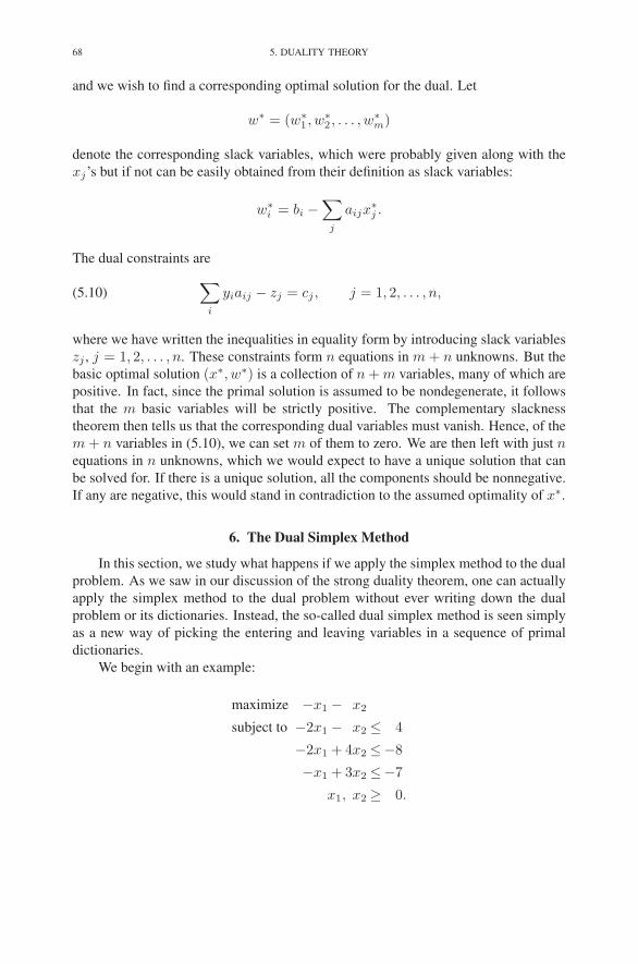
68 5. DUALITY THEORY
and we wish to find a corresponding optimal solution for the dual. Let
w∗ = (w∗1 , w∗
2 , . . . , w∗m)
denote the corresponding slack variables, which were probably given along with the
xj’s but if not can be easily obtained from their definition as slack variables:
w∗i = bi −
∑
j
aijx∗j .
The dual constraints are
(5.10)∑
i
yiaij − zj = cj , j = 1, 2, . . . , n,
where we have written the inequalities in equality form by introducing slack variables
zj , j = 1, 2, . . . , n. These constraints form n equations in m + n unknowns. But the
basic optimal solution (x∗, w∗) is a collection of n + m variables, many of which are
positive. In fact, since the primal solution is assumed to be nondegenerate, it follows
that the m basic variables will be strictly positive. The complementary slackness
theorem then tells us that the corresponding dual variables must vanish. Hence, of the
m + n variables in (5.10), we can set m of them to zero. We are then left with just nequations in n unknowns, which we would expect to have a unique solution that can
be solved for. If there is a unique solution, all the components should be nonnegative.
If any are negative, this would stand in contradiction to the assumed optimality of x∗.
6. The Dual Simplex Method
In this section, we study what happens if we apply the simplex method to the dual
problem. As we saw in our discussion of the strong duality theorem, one can actually
apply the simplex method to the dual problem without ever writing down the dual
problem or its dictionaries. Instead, the so-called dual simplex method is seen simply
as a new way of picking the entering and leaving variables in a sequence of primal
dictionaries.
We begin with an example:
maximize −x1 − x2
subject to −2x1 − x2 ≤ 4
−2x1 + 4x2 ≤−8
−x1 + 3x2 ≤−7
x1, x2 ≥ 0.
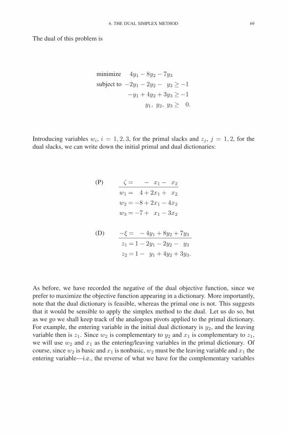
6. THE DUAL SIMPLEX METHOD 69
The dual of this problem is
minimize 4y1 − 8y2 − 7y3
subject to −2y1 − 2y2 − y3 ≥−1
−y1 + 4y2 + 3y3 ≥−1
y1, y2, y3 ≥ 0.
Introducing variables wi, i = 1, 2, 3, for the primal slacks and zj , j = 1, 2, for the
dual slacks, we can write down the initial primal and dual dictionaries:
(P) ζ = − x1 − x2
w1 = 4 + 2x1 + x2
w2 =−8 + 2x1 − 4x2
w3 =−7 + x1 − 3x2
(D) −ξ = − 4y1 + 8y2 + 7y3
z1 = 1− 2y1 − 2y2 − y3
z2 = 1− y1 + 4y2 + 3y3.
As before, we have recorded the negative of the dual objective function, since we
prefer to maximize the objective function appearing in a dictionary. More importantly,
note that the dual dictionary is feasible, whereas the primal one is not. This suggests
that it would be sensible to apply the simplex method to the dual. Let us do so, but
as we go we shall keep track of the analogous pivots applied to the primal dictionary.
For example, the entering variable in the initial dual dictionary is y2, and the leaving
variable then is z1. Since w2 is complementary to y2 and x1 is complementary to z1,
we will use w2 and x1 as the entering/leaving variables in the primal dictionary. Of
course, since w2 is basic and x1 is nonbasic, w2 must be the leaving variable and x1 the
entering variable—i.e., the reverse of what we have for the complementary variables
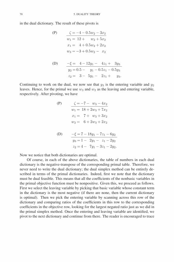
70 5. DUALITY THEORY
in the dual dictionary. The result of these pivots is
(P) ζ =−4− 0.5w2 − 3x2
w1 = 12 + w2 + 5x2
x1 = 4 + 0.5w2 + 2x2
w3 =−3 + 0.5w2 − x2
(D) −ξ = 4− 12y1 − 4z1 + 3y3
y2 = 0.5− y1 − 0.5z1 − 0.5y3
z2 = 3− 5y1 − 2z1 + y3.
Continuing to work on the dual, we now see that y3 is the entering variable and y2
leaves. Hence, for the primal we use w3 and w2 as the leaving and entering variable,
respectively. After pivoting, we have
(P) ζ =−7− w3 − 4x2
w1 = 18 + 2w3 + 7x2
x1 = 7 + w3 + 3x2
w2 = 6 + 2w3 + 2x2
(D) −ξ = 7− 18y1 − 7z1 − 6y2
y3 = 1− 2y1 − z1 − 2y2
z2 = 4− 7y1 − 3z1 − 2y2.
Now we notice that both dictionaries are optimal.
Of course, in each of the above dictionaries, the table of numbers in each dual
dictionary is the negative-transpose of the corresponding primal table. Therefore, we
never need to write the dual dictionary; the dual simplex method can be entirely de-
scribed in terms of the primal dictionaries. Indeed, first we note that the dictionary
must be dual feasible. This means that all the coefficients of the nonbasic variables in
the primal objective function must be nonpositive. Given this, we proceed as follows.
First we select the leaving variable by picking that basic variable whose constant term
in the dictionary is the most negative (if there are none, then the current dictionary
is optimal). Then we pick the entering variable by scanning across this row of the
dictionary and comparing ratios of the coefficients in this row to the corresponding
coefficients in the objective row, looking for the largest negated ratio just as we did in
the primal simplex method. Once the entering and leaving variable are identified, we
pivot to the next dictionary and continue from there. The reader is encouraged to trace
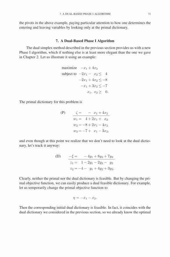
7. A DUAL-BASED PHASE I ALGORITHM 71
the pivots in the above example, paying particular attention to how one determines the
entering and leaving variables by looking only at the primal dictionary.
7. A Dual-Based Phase I Algorithm
The dual simplex method described in the previous section provides us with a new
Phase I algorithm, which if nothing else is at least more elegant than the one we gave
in Chapter 2. Let us illustrate it using an example:
maximize −x1 + 4x2
subject to −2x1 − x2 ≤ 4
−2x1 + 4x2 ≤−8
−x1 + 3x2 ≤−7
x1, x2 ≥ 0.
The primal dictionary for this problem is
(P) ζ = − x1 + 4x2
w1 = 4 + 2x1 + x2
w2 =−8 + 2x1 − 4x2
w3 =−7 + x1 − 3x2,
and even though at this point we realize that we don’t need to look at the dual dictio-
nary, let’s track it anyway:
(D) −ξ = − 4y1 + 8y2 + 7y3
z1 = 1− 2y1 − 2y2 − y3
z2 =−4− y1 + 4y2 + 3y3.
Clearly, neither the primal nor the dual dictionary is feasible. But by changing the pri-
mal objective function, we can easily produce a dual feasible dictionary. For example,
let us temporarily change the primal objective function to
η = −x1 − x2.
Then the corresponding initial dual dictionary is feasible. In fact, it coincides with the
dual dictionary we considered in the previous section, so we already know the optimal

72 5. DUALITY THEORY
solution for this modified problem. The optimal primal dictionary is
η =−7− w3 − 4x2
w1 = 18 + 2w3 + 7x2
x1 = 7 + w3 + 3x2
w2 = 6 + 2w3 + 2x2.
This primal dictionary is optimal for the modified problem but not for the original
problem. However, it is feasible for the original problem, and we can now simply
reinstate the intended objective function and continue with Phase II. Indeed,
ζ =−x1 + 4x2
=−(7 + w3 + 3x2) + 4x2
=−7 − w3 + x2.
Hence, the starting dictionary for Phase II is
ζ =−7− w3 + x2
w1 = 18 + 2w3 + 7x2
x1 = 7 + w3 + 3x2
w2 = 6 + 2w3 + 2x2.
The entering variable is x2. Looking for a leaving variable, we discover that this
problem is unbounded. Of course, more typically one would expect to have to do
several iterations of Phase II to find the optimal solution (or show unboundedness).
Here we just got lucky that the game ended so soon.
It is interesting to note how we detect infeasibility with this new Phase I algorithm.
The modified problem is guaranteed always to be dual feasible. It is easy to see that
the primal problem is infeasible if and only if the modified problem is dual unbounded
(which the dual simplex method will detect just as the primal simplex method detects
primal unboundedness).
The two-phase algorithm we have just presented can be thought of as a dual–
primal algorithm, since we first apply the dual simplex method to a modified dual
feasible problem and then finish off by applying the primal simplex method to the
original problem, starting from the feasible dictionary produced by Phase I. One could
consider turning this around and doing a primal–dual two-phase algorithm. Here, the
right-hand side of the primal problem would be modified to produce an obvious primal
feasible solution. The primal simplex method would then be applied. The optimal
solution to this primal problem will then be feasible for the original dual problem but

8. THE DUAL OF A PROBLEM IN GENERAL FORM 73
will not be optimal for it. But then the dual simplex method can be applied, starting
with this dual feasible basis until an optimal solution for the dual problem is obtained.
8. The Dual of a Problem in General Form
In Chapter 1, we saw that linear programming problems can be formulated in a
variety of ways. In this section, we shall derive the form of the dual when the primal
problem is not necessarily presented in standard form.
First, let us consider the case where the linear constraints are equalities (and the
variables are nonnegative):
(5.11)
maximize
n∑
j=1
cjxj
subject to
n∑
j=1
aijxj = bi i = 1, 2, . . . ,m
xj ≥ 0 j = 1, 2, . . . , n.
As we mentioned in Chapter 1, this problem can be reformulated with inequality con-
straints by simply writing each equality as two inequalities: one greater-than-or-equal-
to and one less-than-or-equal-to:
maximize
n∑
j=1
cjxj
subject to
n∑
j=1
aijxj ≤ bi i = 1, 2, . . . ,m
n∑
j=1
aijxj ≥ bi i = 1, 2, . . . ,m
xj ≥ 0 j = 1, 2, . . . , n.
Then negating each greater-than-or-equal-to constraint, we can put the problem into
standard form:
maximize
n∑
j=1
cjxj
subject to
n∑
j=1
aijxj ≤ bi i = 1, 2, . . . ,m
n∑
j=1
−aijxj ≤ −bi i = 1, 2, . . . ,m
xj ≥ 0 j = 1, 2, . . . , n.
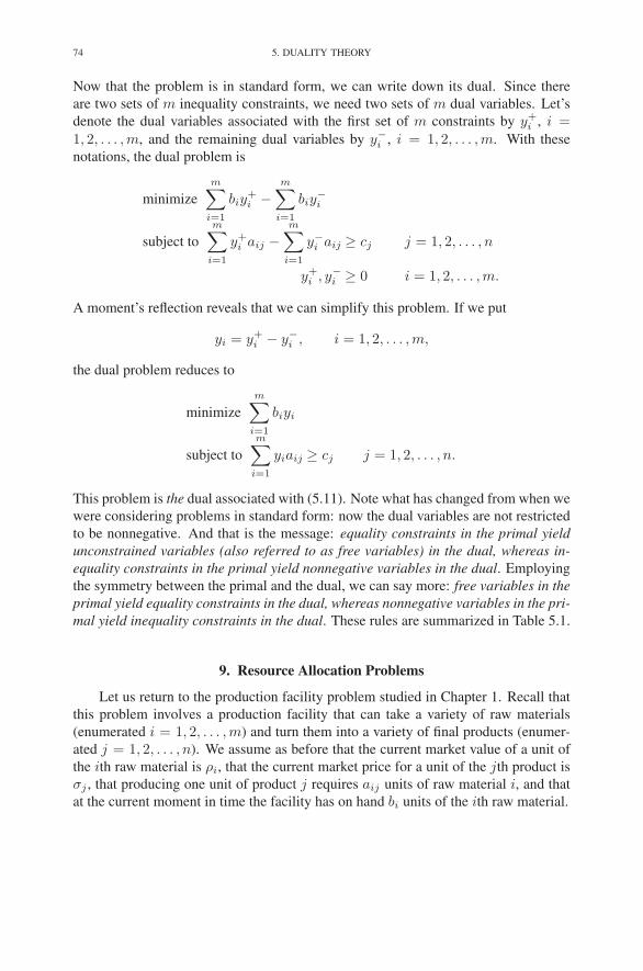
74 5. DUALITY THEORY
Now that the problem is in standard form, we can write down its dual. Since there
are two sets of m inequality constraints, we need two sets of m dual variables. Let’s
denote the dual variables associated with the first set of m constraints by y+i , i =
1, 2, . . . , m, and the remaining dual variables by y−i , i = 1, 2, . . . ,m. With these
notations, the dual problem is
minimize
m∑
i=1
biy+i −
m∑
i=1
biy−i
subject to
m∑
i=1
y+i aij −
m∑
i=1
y−i aij ≥ cj j = 1, 2, . . . , n
y+i , y−
i ≥ 0 i = 1, 2, . . . ,m.
A moment’s reflection reveals that we can simplify this problem. If we put
yi = y+i − y−
i , i = 1, 2, . . . ,m,
the dual problem reduces to
minimize
m∑
i=1
biyi
subject to
m∑
i=1
yiaij ≥ cj j = 1, 2, . . . , n.
This problem is the dual associated with (5.11). Note what has changed from when we
were considering problems in standard form: now the dual variables are not restricted
to be nonnegative. And that is the message: equality constraints in the primal yield
unconstrained variables (also referred to as free variables) in the dual, whereas in-
equality constraints in the primal yield nonnegative variables in the dual. Employing
the symmetry between the primal and the dual, we can say more: free variables in the
primal yield equality constraints in the dual, whereas nonnegative variables in the pri-
mal yield inequality constraints in the dual. These rules are summarized in Table 5.1.
9. Resource Allocation Problems
Let us return to the production facility problem studied in Chapter 1. Recall that
this problem involves a production facility that can take a variety of raw materials
(enumerated i = 1, 2, . . . ,m) and turn them into a variety of final products (enumer-
ated j = 1, 2, . . . , n). We assume as before that the current market value of a unit of
the ith raw material is ρi, that the current market price for a unit of the jth product is
σj , that producing one unit of product j requires aij units of raw material i, and that
at the current moment in time the facility has on hand bi units of the ith raw material.

9. RESOURCE ALLOCATION PROBLEMS 75
Primal Dual
Equality Constraint Free Variable
Inequality Constraint Nonnegative Variable
Free Variable Equality Constraint
Nonnegative Variable Inequality Constraint
TABLE 5.1. Rules for forming the dual.
The current market values/prices are, by definition, related to each other by the
formulas
σj =∑
i
ρiaij , j = 1, 2, . . . , n.
These equations hold whenever the market is in equilibrium. (Of course, it is crucial to
assume here that the collection of “raw materials” appearing on the right-hand side is
exhaustive, including such items as depreciation of fixed assets and physical labor.) In
the real world, the market is always essentially in equilibrium. Nonetheless, it contin-
ually experiences small perturbations that ripple through it and move the equilibrium
to new levels.
These perturbations can be from several causes, an important one being innova-
tion. One possible innovation is to improve the production process. This means that
the values of some of the aij’s are reduced. Now, suddenly there is a windfall profit
for each unit of product j produced. This windfall profit is given by
(5.12) cj = σj −∑
i
ρiaij .
Of course, eventually most producers of these products will take advantage of the same
innovation, and once the suppliers get wind of the profits being made, they will get in
on the action by raising the price of the raw materials.1 Nonetheless, there is always a
time lag; it is during this time that fortunes are made.
To be concrete, let us assume that the time lag is about one month (depending
on the industry, this lag time could be considered too short or too long). Suppose
also that the production manager decides to produce xj units of product j and that
all units produced are sold immediately at their market value. Then the total revenue
1One could take the prices of raw materials as fixed and argue that the value of the final products will
fall. It doesn’t really matter which view one adopts, since prices are relative anyway. The point is simply
that the difference between the price of the raw materials and the price of the final products must narrow
due to this innovation.

76 5. DUALITY THEORY
during this month will be∑
j σjxj . The value of the raw materials on hand at the
beginning of the month was∑
i ρibi. Also, if we denote the new price levels for the
raw materials at the end of the month by wi, i = 1, 2, . . . ,m, then the value of any
remaining inventory at the end of the month is given by
∑
i
wi
⎛
⎝bi −∑
j
aijxj
⎞
⎠
(if any term is negative, then it represents the cost of purchasing additional raw mate-
rials to meet the month’s production requirements—we assume that these additional
purchases are made at the new, higher, end-of-month price). The total windfall, call it
π, (over all products) for this month can now be written as
(5.13) π =∑
j
σjxj +∑
i
wi
⎛
⎝bi −∑
j
aijxj
⎞
⎠−∑
i
ρibi.
Our aim is to choose production levels xj , j = 1, 2, . . . , n, that maximize this
windfall. But our supplier’s aim is to choose prices wi, i = 1, 2, . . . , m, so as to
minimize our windfall. Before studying these optimizations, let us first rewrite the
windfall in a more convenient form. As in Chapter 1, let yi denote the increase in the
price of raw material i. That is,
(5.14) wi = ρi + yi.
Substituting (5.14) into (5.13) and then simplifying notations using (5.12), we see that
(5.15) π =∑
j
cjxj +∑
i
yi
⎛
⎝bi −∑
j
aijxj
⎞
⎠ .
To emphasize that π depends on each of the xj’s and on the yi’s, we sometimes write
it as π(x1, . . . , xn, y1, . . . , ym).Now let us return to the competing optimizations. Given xj for j = 1, 2, . . . , n,
the suppliers react to minimize π(x1, . . . , xn, y1, . . . , ym). Looking at (5.15), we see
that for any resource i in short supply, that is,
bi −∑
j
aijxj < 0,

9. RESOURCE ALLOCATION PROBLEMS 77
the suppliers will jack up the price immensely (i.e., yi = ∞). To avoid this obviously
bad situation, the production manager will be sure to set the production levels so that
∑
j
aijxj ≤ bi, i = 1, 2, . . . , m.
On the other hand, for any resource i that is not exhausted during the windfall month,
that is,
bi −∑
j
aijxj > 0,
the suppliers will have no incentive to change the prevailing market price (i.e., yi = 0).
Therefore, from the production manager’s point of view, the problem reduces to one
of maximizing∑
j
cjxj
subject to the constraints that
∑
j
aijxj ≤ bi, i = 1, 2, . . . ,m,
xj ≥ 0, j = 1, 2, . . . , n.
This is just our usual primal linear programming problem. This is the problem that the
production manager needs to solve in anticipation of adversarial suppliers.
Now let us look at the problem from the suppliers’ point of view. Rearranging the
terms in (5.15) by writing
(5.16) π =∑
j
(
cj −∑
i
yiaij
)
xj +∑
i
yibi,
we see that if the suppliers set prices in such a manner that a windfall remains on the
jth product even after the price adjustment, that is,
cj −∑
i
yiaij > 0,
then the production manager would be able to generate for the facility an arbitrarily
large windfall by producing a huge amount of the jth product (i.e., xj = ∞). We
assume that this is unacceptable to the suppliers, and so they will determine their price
increases so that∑
i
yiaij ≥ cj , j = 1, 2, . . . , n.

78 5. DUALITY THEORY
Also, if the suppliers set the price increases too high so that the production facility will
lose money by producing product j, that is,
cj −∑
i
yiaij < 0,
then the production manager would simply decide not to engage in that activity. That
is, she would set xj = 0. Hence, the first term in (5.16) will always be zero, and so
the optimization problem faced by the suppliers is to minimize
∑
i
biyi
subject to the constraints that
∑
i
yiaij ≥ cj , j = 1, 2, . . . , n,
yi ≥ 0, i = 1, 2, . . . ,m.
This is precisely the dual of the production manager’s problem!
As we’ve seen earlier with the strong duality theorem, if the production manager’s
problem has an optimal solution, then so does the suppliers’ problem, and the two
objectives agree. This means than an equilibrium can be reestablished by setting the
production levels and the price hikes according to the optimal solutions to these two
linear programming problems.
10. Lagrangian Duality
The analysis of the preceding section is an example of a general technique that
forms the foundation of a subject called Lagrangian duality, which we shall briefly
describe.
Let us start by summarizing what we did. It was quite simple. The analysis
revolved around a function
π(x1, . . . , xn, y1, . . . , ym) =∑
j
cjxj −∑
i
∑
j
yiaijxj +∑
i
yibi.
To streamline notations, let x stand for the entire collection of variables x1, x2, . . . , xn
and let y stand for the collection of yi’s so that we can write π(x, y) in place of
π(x1, . . . , xn, y1, . . . , ym). Written with these notations, we showed in the previous
section that
maxx≥0
miny≥0
π(x, y) = miny≥0
maxx≥0
π(x, y).
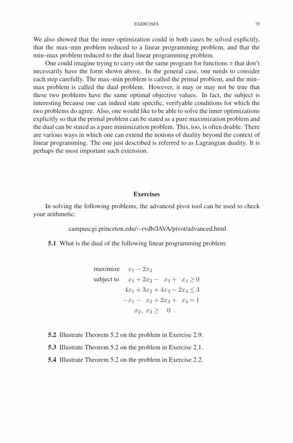
EXERCISES 79
We also showed that the inner optimization could in both cases be solved explicitly,
that the max–min problem reduced to a linear programming problem, and that the
min–max problem reduced to the dual linear programming problem.
One could imagine trying to carry out the same program for functions π that don’t
necessarily have the form shown above. In the general case, one needs to consider
each step carefully. The max–min problem is called the primal problem, and the min–
max problem is called the dual problem. However, it may or may not be true that
these two problems have the same optimal objective values. In fact, the subject is
interesting because one can indeed state specific, verifyable conditions for which the
two problems do agree. Also, one would like to be able to solve the inner optimizations
explicitly so that the primal problem can be stated as a pure maximization problem and
the dual can be stated as a pure minimization problem. This, too, is often doable. There
are various ways in which one can extend the notions of duality beyond the context of
linear programming. The one just described is referred to as Lagrangian duality. It is
perhaps the most important such extension.
Exercises
In solving the following problems, the advanced pivot tool can be used to check
your arithmetic:
campuscgi.princeton.edu/∼rvdb/JAVA/pivot/advanced.html
5.1 What is the dual of the following linear programming problem:
maximize x1 − 2x2
subject to x1 + 2x2 − x3 + x4 ≥ 0
4x1 + 3x2 + 4x3 − 2x4 ≤ 3
−x1 − x2 + 2x3 + x4 = 1
x2, x3 ≥ 0 .
5.2 Illustrate Theorem 5.2 on the problem in Exercise 2.9.
5.3 Illustrate Theorem 5.2 on the problem in Exercise 2.1.
5.4 Illustrate Theorem 5.2 on the problem in Exercise 2.2.
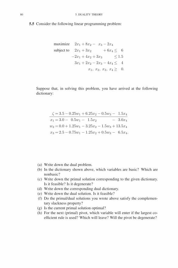
80 5. DUALITY THEORY
5.5 Consider the following linear programming problem:
maximize 2x1 + 8x2 − x3 − 2x4
subject to 2x1 + 3x2 + 6x4 ≤ 6
−2x1 + 4x2 + 3x3 ≤ 1.5
3x1 + 2x2 − 2x3 − 4x4 ≤ 4
x1, x2, x3, x4 ≥ 0.
Suppose that, in solving this problem, you have arrived at the following
dictionary:
ζ = 3.5− 0.25w1 + 6.25x2 − 0.5w3 − 1.5x4
x1 = 3.0− 0.5w1 − 1.5x2 − 3.0x4
w2 = 0.0 + 1.25w1 − 3.25x2 − 1.5w3 + 13.5x4
x3 = 2.5− 0.75w1 − 1.25x2 + 0.5w3 − 6.5x4.
(a) Write down the dual problem.
(b) In the dictionary shown above, which variables are basic? Which are
nonbasic?
(c) Write down the primal solution corresponding to the given dictionary.
Is it feasible? Is it degenerate?
(d) Write down the corresponding dual dictionary.
(e) Write down the dual solution. Is it feasible?
(f) Do the primal/dual solutions you wrote above satisfy the complemen-
tary slackness property?
(g) Is the current primal solution optimal?
(h) For the next (primal) pivot, which variable will enter if the largest co-
efficient rule is used? Which will leave? Will the pivot be degenerate?
EXERCISES 81
5.6 Solve the following linear program:
maximize −x1 − 2x2
subject to −2x1 + 7x2 ≤ 6
−3x1 + x2 ≤−1
9x1 − 4x2 ≤ 6
x1 − x2 ≤ 1
7x1 − 3x2 ≤ 6
−5x1 + 2x2 ≤−3
x1, x2 ≥ 0.
5.7 Solve the linear program given in Exercise 2.3 using the dual–primal two-
phase algorithm.
5.8 Solve the linear program given in Exercise 2.4 using the dual–primal two-
phase algorithm.
5.9 Solve the linear program given in Exercise 2.6 using the dual–primal two-
phase algorithm.
5.10 Using today’s date (MMYY) for the seed value, solve 10 problems using the
dual phase I primal phase II simplex method:
campuscgi.princeton.edu/∼rvdb/JAVA/pivot/dp2phase.html .
5.11 Using today’s date (MMYY) for the seed value, solve 10 problems using the
primal phase I dual phase II simplex method:
campuscgi.princeton.edu/∼rvdb/JAVA/pivot/pd2phase.html
5.12 For x and y in R, compute
maxx≥0
miny≥0
(x − y) and miny≥0
maxx≥0
(x − y)
and note whether or not they are equal.
82 5. DUALITY THEORY
5.13 Consider the following process. Starting with a linear programming problem
in standard form,
maximize
n∑
j=1
cjxj
subject to
n∑
j=1
aijxj ≤ bi i = 1, 2, . . . ,m
xj ≥ 0 j = 1, 2, . . . , n,
first form its dual:
minimize
m∑
i=1
biyi
subject to
m∑
i=1
yiaij ≥ cj j = 1, 2, . . . , n
yi ≥ 0 i = 1, 2, . . . ,m.
Then replace the minimization in the dual with a maximization to get a new
linear programming problem, which we can write in standard form as fol-
lows:
maximize
m∑
i=1
biyi
subject to
m∑
i=1
−yiaij ≤ −cj j = 1, 2, . . . , n
yi ≥ 0 i = 1, 2, . . . ,m.
If we identify a linear programming problem with its data, (aij , bi, cj), the
above process can be thought of as a transformation T on the space of data
defined by
(aij , bi, cj)T−→ (−aji,−cj , bi).
Let ζ∗(aij , bi, cj) denote the optimal objective function value of the standard-
form linear programming problem having data (aij , bi, cj). By strong dual-
ity together with the fact that a maximization dominates a minimization, it
follows that
ζ∗(aij , bi, cj) ≤ ζ∗(−aji,−cj , bi).
EXERCISES 83
Now if we repeat this process, we get
(aij , bi, cj)T→ (−aji,−cj , bi)
T→ (aij ,−bi,−cj)
T→ (−aji, cj ,−bi)
T→ (aij , bi, cj)
and hence that
ζ∗(aij , bi, cj)≤ ζ∗(−aji,−cj , bi)
≤ ζ∗(aij ,−bi,−cj)
≤ ζ∗(−aji, cj ,−bi)
≤ ζ∗(aij , bi, cj).
But the first and the last entry in this chain of inequalities are equal. There-
fore, all these inequalities would seem to be equalities. While this outcome
could happen sometimes, it certainly isn’t always true. What is the error in
this logic? Can you state a (correct) nontrivial theorem that follows from
this line of reasoning? Can you give an example where the four inequalities
are indeed all equalities?
5.14 Consider the following variant of the resource allocation problem:
(5.17)
maximize
n∑
j=1
cjxj
subject to
n∑
j=1
aijxj ≤ bi i = 1, 2, . . . ,m
0 ≤ xj ≤ uj j = 1, 2, . . . , n.
As usual, the cj’s denote the unit prices for the products and the bi’s denote
the number of units on hand for each raw material. In this variant, the uj’s
denote upper bounds on the number of units of each product that can be
sold at the set price. Now, let’s assume that the raw materials have not
been purchased yet and it is part of the problem to determine the bi’s. Let
pi, i = 1, 2, . . . ,m denote the price for raw material i. The problem then
84 5. DUALITY THEORY
becomes an optimization over both the xj’s and the bi’s:
maximize
n∑
j=1
cjxj −m∑
i=1
pibi
subject to
n∑
j=1
aijxj − bi ≤ 0 i = 1, 2, . . . ,m
0 ≤ xj ≤ uj j = 1, 2, . . . , n
bi ≥ 0 i = 1, 2, . . . ,m.
(a) Show that this problem always has an optimal solution.
(b) Let y∗i (b), i = 1, 2, . . . , m, denote optimal dual variables for the origi-
nal resource allocation problem (5.17). Note that we’ve explicitly indi-
cated that these dual variables depend on the b’s. Also, we assume that
problem (5.17) is both primal and dual non-degenerate so the y∗i (b) is
uniquely defined. Show that the optimal value of the bi’s, call them
b∗i ’s, satisfy
y∗i (b∗) = pi.
Hint: You will need to use the fact that, for resource allocation prob-
lems, we have aij ≥ 0 for all i, and all j.
5.15 Consider the following linear program:
maximize
n∑
j=1
pjxj
subject to
n∑
j=1
qjxj ≤ β
xj ≤ 1 j = 1, 2, . . . , n
xj ≥ 0 j = 1, 2, . . . , n.
Here, the numbers pj , j = 1, 2, . . . , n are positive and sum to one. The same
is true of the qj’s:
n∑
j=1
qj = 1
qj > 0.
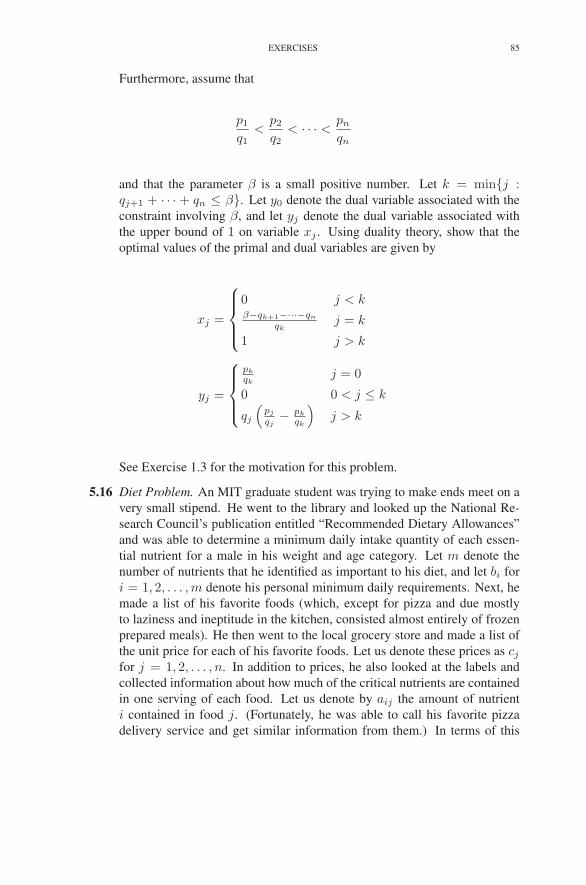
EXERCISES 85
Furthermore, assume that
p1
q1<
p2
q2< · · · <
pn
qn
and that the parameter β is a small positive number. Let k = min{j :qj+1 + · · · + qn ≤ β}. Let y0 denote the dual variable associated with the
constraint involving β, and let yj denote the dual variable associated with
the upper bound of 1 on variable xj . Using duality theory, show that the
optimal values of the primal and dual variables are given by
xj =
⎧
⎪
⎪
⎨
⎪
⎪
⎩
0 j < kβ−qk+1−···−qn
qkj = k
1 j > k
yj =
⎧
⎪
⎪
⎨
⎪
⎪
⎩
pk
qkj = 0
0 0 < j ≤ k
qj
(
pj
qj− pk
qk
)
j > k
See Exercise 1.3 for the motivation for this problem.
5.16 Diet Problem. An MIT graduate student was trying to make ends meet on a
very small stipend. He went to the library and looked up the National Re-
search Council’s publication entitled “Recommended Dietary Allowances”
and was able to determine a minimum daily intake quantity of each essen-
tial nutrient for a male in his weight and age category. Let m denote the
number of nutrients that he identified as important to his diet, and let bi for
i = 1, 2, . . . , m denote his personal minimum daily requirements. Next, he
made a list of his favorite foods (which, except for pizza and due mostly
to laziness and ineptitude in the kitchen, consisted almost entirely of frozen
prepared meals). He then went to the local grocery store and made a list of
the unit price for each of his favorite foods. Let us denote these prices as cj
for j = 1, 2, . . . , n. In addition to prices, he also looked at the labels and
collected information about how much of the critical nutrients are contained
in one serving of each food. Let us denote by aij the amount of nutrient
i contained in food j. (Fortunately, he was able to call his favorite pizza
delivery service and get similar information from them.) In terms of this

86 5. DUALITY THEORY
information, he formulated the following linear programming problem:
minimize
n∑
j=1
cjxj
subject to
n∑
j=1
aijxj ≥ bi i = 1, 2, . . . ,m
xj ≥ 0 j = 1, 2, . . . , n.
Formulate the dual to this linear program. Can you introduce another person
into the above story whose problem would naturally be to solve the dual?
5.17 Saddle points. A function h(y) defined for y ∈ R is called strongly convex
if
• h′′(y) > 0 for all y ∈ R,
• limy→−∞ h′(y) = −∞, and
• limy→∞ h′(y) = ∞.
A function h is called strongly concave if −h is strongly convex. Let π(x, y),be a function defined for (x, y) ∈ R
2 and having the following form
π(x, y) = f(x) − xy + g(y),
where f is strongly concave and g is strongly convex. Using elementary
calculus
1. Show that there is one and only one point (x∗, y∗) ∈ R2 at which the
gradient of π,
∇π =
[
∂π/∂x
∂π/∂y
]
,
vanishes. Hint: From the two equations obtained by setting the deriva-
tives to zero, derive two other relations having the form x = φ(x) and
y = ψ(y). Then study the functions φ and ψ to show that there is one
and only one solution.
2. Show that
maxx∈R
miny∈R
π(x, y) = π(x∗, y∗) = miny∈R
maxx∈R
π(x, y),
where (x∗, y∗) denotes the “critical point” identified in part 1 above.
(Note: Be sure to check the signs of the second derivatives for both the
inner and the outer optimizations.)
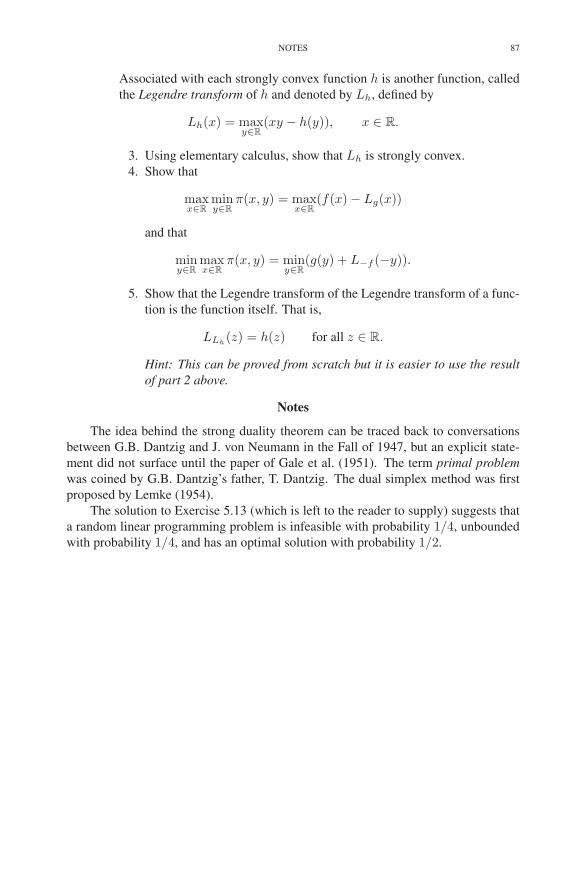
NOTES 87
Associated with each strongly convex function h is another function, called
the Legendre transform of h and denoted by Lh, defined by
Lh(x) = maxy∈R
(xy − h(y)), x ∈ R.
3. Using elementary calculus, show that Lh is strongly convex.
4. Show that
maxx∈R
miny∈R
π(x, y) = maxx∈R
(f(x) − Lg(x))
and that
miny∈R
maxx∈R
π(x, y) = miny∈R
(g(y) + L−f (−y)).
5. Show that the Legendre transform of the Legendre transform of a func-
tion is the function itself. That is,
LLh(z) = h(z) for all z ∈ R.
Hint: This can be proved from scratch but it is easier to use the result
of part 2 above.
Notes
The idea behind the strong duality theorem can be traced back to conversations
between G.B. Dantzig and J. von Neumann in the Fall of 1947, but an explicit state-
ment did not surface until the paper of Gale et al. (1951). The term primal problem
was coined by G.B. Dantzig’s father, T. Dantzig. The dual simplex method was first
proposed by Lemke (1954).
The solution to Exercise 5.13 (which is left to the reader to supply) suggests that
a random linear programming problem is infeasible with probability 1/4, unbounded
with probability 1/4, and has an optimal solution with probability 1/2.


CHAPTER 6
The Simplex Method in Matrix Notation
So far, we have avoided using matrix notation to present linear programming
problems and the simplex method. In this chapter, we shall recast everything into
matrix notation. At the same time, we will emphasize the close relations between the
primal and the dual problems.
1. Matrix Notation
As usual, we begin our discussion with the standard-form linear programming
problem:
maximize
n∑
j=1
cjxj
subject to
n∑
j=1
aijxj ≤ bi i = 1, 2, . . . ,m
xj ≥ 0 j = 1, 2, . . . , n.
In the past, we have generally denoted slack variables by wi’s but have noted that
sometimes it is convenient just to string them onto the end of the list of original vari-
ables. Such is the case now, and so we introduce slack variables as follows:
xn+i = bi −n
∑
j=1
aijxj , i = 1, 2, . . . ,m.
With these slack variables, we now write our problem in matrix form:
maximize cT x
subject to Ax = b
x≥ 0,
89

90 6. THE SIMPLEX METHOD IN MATRIX NOTATION
where
(6.1) A =
⎡
⎢
⎢
⎢
⎢
⎢
⎣
a11 a12 . . . a1n 1
a21 a22 . . . a2n 1...
......
. . .
am1 am2 . . . amn 1
⎤
⎥
⎥
⎥
⎥
⎥
⎦
,
(6.2) b =
⎡
⎢
⎢
⎢
⎢
⎢
⎣
b1
b2
...
bm
⎤
⎥
⎥
⎥
⎥
⎥
⎦
, c =
⎡
⎢
⎢
⎢
⎢
⎢
⎢
⎢
⎢
⎢
⎢
⎢
⎢
⎢
⎣
c1
c2
...
cn
0...
0
⎤
⎥
⎥
⎥
⎥
⎥
⎥
⎥
⎥
⎥
⎥
⎥
⎥
⎥
⎦
, and x =
⎡
⎢
⎢
⎢
⎢
⎢
⎢
⎢
⎢
⎢
⎢
⎢
⎢
⎢
⎣
x1
x2
...
xn
xn+1
...
xn+m
⎤
⎥
⎥
⎥
⎥
⎥
⎥
⎥
⎥
⎥
⎥
⎥
⎥
⎥
⎦
.
As we know, the simplex method is an iterative procedure in which each iteration
is characterized by specifying which m of the n + m variables are basic. As before,
we denote by B the set of indices corresponding to the basic variables, and we denote
by N the remaining nonbasic indices.
In component notation, the ith component of Ax can be broken up into a basic
part and a nonbasic part:
(6.3)
n+m∑
j=1
aijxj =∑
j∈Baijxj +
∑
j∈Naijxj .
We wish to introduce a notation for matrices that will allow us to break up the matrix
product Ax analogously. To this end, let B denote an m × m matrix whose columns
consist precisely of the m columns of A that are associated with the basic variables.
Similarly, let N denote an m × n matrix whose columns are the n nonbasic columns
of A. Then we write A in a partitioned-matrix form as follows:
A =[
B N]
Strictly speaking, the matrix on the right does not equal the A matrix. Instead, it is the
A matrix with its columns rearranged in such a manner that all the columns associated
with basic variables are listed first followed by the nonbasic columns. Nonetheless, as
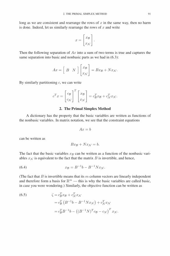
2. THE PRIMAL SIMPLEX METHOD 91
long as we are consistent and rearrange the rows of x in the same way, then no harm
is done. Indeed, let us similarly rearrange the rows of x and write
x =
[
xB
xN
]
.
Then the following separation of Ax into a sum of two terms is true and captures the
same separation into basic and nonbasic parts as we had in (6.3):
Ax =[
B N]
[
xB
xN
]
= BxB + NxN .
By similarly partitioning c, we can write
cT x =
[
cB
cN
]T [
xB
xN
]
= cTBxB + cT
NxN .
2. The Primal Simplex Method
A dictionary has the property that the basic variables are written as functions of
the nonbasic variables. In matrix notation, we see that the constraint equations
Ax = b
can be written as
BxB + NxN = b.
The fact that the basic variables xB can be written as a function of the nonbasic vari-
ables xN is equivalent to the fact that the matrix B is invertible, and hence,
(6.4) xB = B−1b − B−1NxN .
(The fact that B is invertible means that its m column vectors are linearly independent
and therefore form a basis for Rm — this is why the basic variables are called basic,
in case you were wondering.) Similarly, the objective function can be written as
ζ = cTBxB + cT
NxN(6.5)
= cTB(
B−1b − B−1NxN)
+ cTNxN
= cTBB−1b −
(
(B−1N)T cB − cN)T
xN .

92 6. THE SIMPLEX METHOD IN MATRIX NOTATION
Combining (6.5) and (6.4), we see that we can write the dictionary associated with
basis B as
(6.6)ζ = cT
BB−1b−(
(B−1N)T cB − cN)T
xN
xB = B−1b−B−1NxN .
Comparing against the component-form notation of Chapter 2 (see (2.6)), we make
the following identifications:
cTBB−1b = ζ
cN − (B−1N)T cB = [cj ]
B−1b =[
bi
]
B−1N = [aij ] ,
where the bracketed expressions on the right denote vectors and matrices with the
index i running over B and the index j running over N . The basic solution associated
with dictionary (6.6) is obtained by setting xN equal to zero:
x∗N = 0,
x∗B = B−1b.(6.7)
As we saw in the last chapter, associated with each primal dictionary there is a
dual dictionary that is simply the negative-transpose of the primal. However, to have
the negative-transpose property, it is important to correctly associate complementary
pairs of variables. So first we recall that, for the current discussion, we have appended
the primal slack variables to the end of the original variables:
(x1, . . . , xn, w1, . . . , wm) −→ (x1, . . . , xn, xn+1, . . . , xn+m).
Also recall that the dual slack variables are complementary to the original primal
variables and that the original dual variables are complementary to the primal slack
variables. Therefore, to maintain the desired complementarity condition between like
indices in the primal and the dual, we need to relabel the dual variables and append
them to the end of the dual slacks:
(z1, . . . , zn, y1, . . . , ym) −→ (z1, . . . , zn, zn+1, . . . , zn+m).
With this relabeling of the dual variables, the dual dictionary corresponding to (6.6) is
−ξ = −cTBB−1b− (B−1b)T zB
zN = (B−1N)T cB − cN + (B−1N)T zB.

2. THE PRIMAL SIMPLEX METHOD 93
The dual solution associated with this dictionary is obtained by setting zB equal to
zero:
z∗B = 0,
z∗N = (B−1N)T cB − cN .(6.8)
Using (6.7) and (6.8) and introducing the shorthand
(6.9) ζ∗ = cTBB−1b,
we see that we can write the primal dictionary succinctly as
(6.10)ζ = ζ∗ − z∗N
T xN
xB = x∗B −B−1NxN .
The associated dual dictionary then has a very symmetric appearance:
(6.11)−ξ =−ζ∗ − (x∗
B)T zB
zN = z∗N + (B−1N)T zB.
The (primal) simplex method can be described briefly as follows. The starting
assumptions are that we are given
(1) a partition of the n + m indices into a collection B of m basic indices and a
collection N of n nonbasic ones with the property that the basis matrix B is
invertible,
(2) an associated current primal solution x∗B ≥ 0 (and x∗
N = 0), and
(3) an associated current dual solution z∗N (with z∗B = 0)
such that the dictionary given by (6.10) represents the primal objective function and
the primal constraints. The simplex method then produces a sequence of steps to
“adjacent” bases such that the current value ζ∗ of the objective function ζ increases
at each step (or, at least, would increase if the step size were positive), updating x∗B
and z∗N along the way. Two bases are said to be adjacent to each other if they differ in
only one index. That is, given a basis B, an adjacent basis is determined by removing
one basic index and replacing it with a nonbasic index. The index that gets removed
corresponds to the leaving variable, whereas the index that gets added corresponds to
the entering variable.
One step of the simplex method is called an iteration. We now elaborate further
on the details by describing one iteration as a sequence of specific steps.
Step 1. Check for Optimality. If z∗N ≥ 0, stop. The current solution is optimal.
To see this, first note that the simplex method always maintains primal feasibility and
complementarity. Indeed, the primal solution is feasible, since x∗B ≥ 0 and xN = 0
and the dictionary embodies the primal constraints. Also, the fact that x∗N = 0 and

94 6. THE SIMPLEX METHOD IN MATRIX NOTATION
z∗B = 0 implies that the primal and dual solutions are complementary. Hence, all that
is required for optimality is dual feasibility. But by looking at the associated dual
dictionary (6.11), we see that the dual solution is feasible if and only if z∗N ≥ 0.
Step 2. Select Entering Variable. Pick an index j ∈ N for which z∗j < 0. Variable
xj is the entering variable.
Step 3. Compute Primal Step Direction ∆xB. Having selected the entering vari-
able, it is our intention to let its value increase from zero. Hence, we let
xN =
⎡
⎢
⎢
⎢
⎢
⎢
⎢
⎢
⎢
⎢
⎢
⎢
⎢
⎢
⎣
0...
0
t
0...
0
⎤
⎥
⎥
⎥
⎥
⎥
⎥
⎥
⎥
⎥
⎥
⎥
⎥
⎥
⎦
տ= tej ,
jth position
where we follow the common convention of letting ej denote the unit vector that is
zero in every component except for a one in the position associated with index j (note
that, because of our index rearrangement conventions, this is not generally the jth
element of the vector). Then from (6.10), we have that
xB = x∗B − B−1Ntej .
Hence, we see that the step direction ∆xB for the primal basic variables is given by
∆xB = B−1Nej .
Step 4. Compute Primal Step Length. We wish to pick the largest t ≥ 0 for which
every component of xB remains nonnegative. That is, we wish to pick the largest t for
which
x∗B ≥ t∆xB.
Since, for each i ∈ B∗, x∗i ≥ 0 and t ≥ 0, we can divide both sides of the above
inequality by these numbers and preserve the sense of the inequality. Therefore, doing
this division, we get the requirement that
1
t≥ ∆xi
x∗i
, for all i ∈ B.
We want to let t be as large as possible, and so 1/t should be made as small as pos-
sible. The smallest possible value for 1/t that satisfies all the required inequalities is
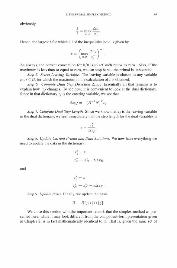
2. THE PRIMAL SIMPLEX METHOD 95
obviously1
t= max
i∈B∆xi
x∗i
.
Hence, the largest t for which all of the inequalities hold is given by
t =
(
maxi∈B
∆xi
x∗i
)−1
.
As always, the correct convention for 0/0 is to set such ratios to zero. Also, if the
maximum is less than or equal to zero, we can stop here—the primal is unbounded.
Step 5. Select Leaving Variable. The leaving variable is chosen as any variable
xi, i ∈ B, for which the maximum in the calculation of t is obtained.
Step 6. Compute Dual Step Direction ∆zN . Essentially all that remains is to
explain how z∗N changes. To see how, it is convenient to look at the dual dictionary.
Since in that dictionary zi is the entering variable, we see that
∆zN = −(B−1N)T ei.
Step 7. Compute Dual Step Length. Since we know that zj is the leaving variable
in the dual dictionary, we see immediately that the step length for the dual variables is
s =z∗j
∆zj.
Step 8. Update Current Primal and Dual Solutions. We now have everything we
need to update the data in the dictionary:
x∗j ← t
x∗B ← x∗
B − t∆xB
and
z∗i ← s
z∗N ← z∗N − s∆zN .
Step 9. Update Basis. Finally, we update the basis:
B ← B \ {i} ∪ {j}.
We close this section with the important remark that the simplex method as pre-
sented here, while it may look different from the component-form presentation given
in Chapter 2, is in fact mathematically identical to it. That is, given the same set of
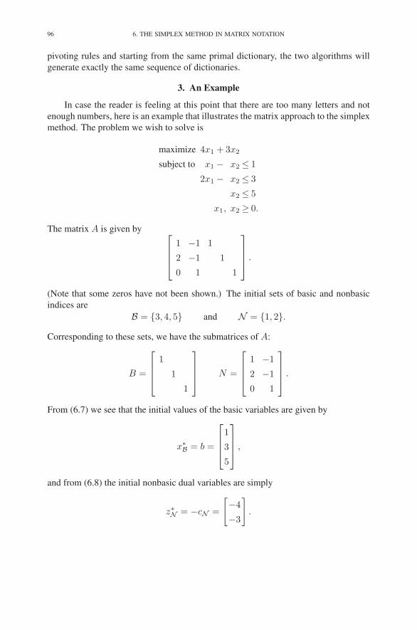
96 6. THE SIMPLEX METHOD IN MATRIX NOTATION
pivoting rules and starting from the same primal dictionary, the two algorithms will
generate exactly the same sequence of dictionaries.
3. An Example
In case the reader is feeling at this point that there are too many letters and not
enough numbers, here is an example that illustrates the matrix approach to the simplex
method. The problem we wish to solve is
maximize 4x1 + 3x2
subject to x1 − x2 ≤ 1
2x1 − x2 ≤ 3
x2 ≤ 5
x1, x2 ≥ 0.
The matrix A is given by⎡
⎢
⎢
⎣
1 −1 1
2 −1 1
0 1 1
⎤
⎥
⎥
⎦
.
(Note that some zeros have not been shown.) The initial sets of basic and nonbasic
indices are
B = {3, 4, 5} and N = {1, 2}.
Corresponding to these sets, we have the submatrices of A:
B =
⎡
⎢
⎢
⎣
1
1
1
⎤
⎥
⎥
⎦
N =
⎡
⎢
⎢
⎣
1 −1
2 −1
0 1
⎤
⎥
⎥
⎦
.
From (6.7) we see that the initial values of the basic variables are given by
x∗B = b =
⎡
⎢
⎢
⎣
1
3
5
⎤
⎥
⎥
⎦
,
and from (6.8) the initial nonbasic dual variables are simply
z∗N = −cN =
[
−4
−3
]
.

3. AN EXAMPLE 97
Since x∗B ≥ 0, the initial solution is primal feasible, and hence we can apply the
simplex method without needing any Phase I procedure.
3.1. First Iteration. Step 1. Since z∗N has some negative components, the cur-
rent solution is not optimal.
Step 2. Since z∗1 = −4 and this is the most negative of the two nonbasic dual
variables, we see that the entering index is
j = 1.
Step 3.
∆xB = B−1Nej =
⎡
⎢
⎢
⎣
1 −1
2 −1
0 1
⎤
⎥
⎥
⎦
[
1
0
]
=
⎡
⎢
⎢
⎣
1
2
0
⎤
⎥
⎥
⎦
.
Step 4.
t =
(
max
{
1
1,2
3,0
5
})−1
= 1.
Step 5. Since the ratio that achieved the maximum in Step 4 was the first ratio and
this ratio corresponds to basis index 3, we see that
i = 3.
Step 6.
∆zN = −(B−1N)T ei = −[
1 2 0
−1 −1 1
]
⎡
⎢
⎢
⎣
1
0
0
⎤
⎥
⎥
⎦
=
[
−1
1
]
.
Step 7.
s =z∗j
∆zj=
−4
−1= 4.
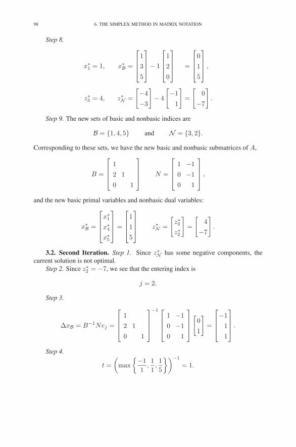
98 6. THE SIMPLEX METHOD IN MATRIX NOTATION
Step 8.
x∗1 = 1, x∗
B =
⎡
⎢
⎢
⎣
1
3
5
⎤
⎥
⎥
⎦
− 1
⎡
⎢
⎢
⎣
1
2
0
⎤
⎥
⎥
⎦
=
⎡
⎢
⎢
⎣
0
1
5
⎤
⎥
⎥
⎦
,
z∗3 = 4, z∗N =
[
−4
−3
]
− 4
[
−1
1
]
=
[
0
−7
]
.
Step 9. The new sets of basic and nonbasic indices are
B = {1, 4, 5} and N = {3, 2}.
Corresponding to these sets, we have the new basic and nonbasic submatrices of A,
B =
⎡
⎢
⎢
⎣
1
2 1
0 1
⎤
⎥
⎥
⎦
N =
⎡
⎢
⎢
⎣
1 −1
0 −1
0 1
⎤
⎥
⎥
⎦
,
and the new basic primal variables and nonbasic dual variables:
x∗B =
⎡
⎢
⎢
⎣
x∗1
x∗4
x∗5
⎤
⎥
⎥
⎦
=
⎡
⎢
⎢
⎣
1
1
5
⎤
⎥
⎥
⎦
z∗N =
[
z∗3z∗2
]
=
[
4
−7
]
.
3.2. Second Iteration. Step 1. Since z∗N has some negative components, the
current solution is not optimal.
Step 2. Since z∗2 = −7, we see that the entering index is
j = 2.
Step 3.
∆xB = B−1Nej =
⎡
⎢
⎢
⎣
1
2 1
0 1
⎤
⎥
⎥
⎦
−1 ⎡
⎢
⎢
⎣
1 −1
0 −1
0 1
⎤
⎥
⎥
⎦
[
0
1
]
=
⎡
⎢
⎢
⎣
−1
1
1
⎤
⎥
⎥
⎦
.
Step 4.
t =
(
max
{−1
1,1
1,1
5
})−1
= 1.

3. AN EXAMPLE 99
Step 5. Since the ratio that achieved the maximum in Step 4 was the second ratio
and this ratio corresponds to basis index 4, we see that
i = 4.
Step 6.
∆zN =−(B−1N)T ei
=−[
1 0 0
−1 −1 1
]
⎡
⎢
⎢
⎣
1 2 0
1
1
⎤
⎥
⎥
⎦
−1 ⎡
⎢
⎢
⎣
0
1
0
⎤
⎥
⎥
⎦
=
[
2
−1
]
.
Step 7.
s =z∗j
∆zj=
−7
−1= 7.
Step 8.
x∗2 = 1, x∗
B =
⎡
⎢
⎢
⎣
1
1
5
⎤
⎥
⎥
⎦
− 1
⎡
⎢
⎢
⎣
−1
1
1
⎤
⎥
⎥
⎦
=
⎡
⎢
⎢
⎣
2
0
4
⎤
⎥
⎥
⎦
,
z∗4 = 7, z∗N =
[
4
−7
]
− 7
[
2
−1
]
=
[
−10
0
]
.
Step 9. The new sets of basic and nonbasic indices are
B = {1, 2, 5} and N = {3, 4}.
Corresponding to these sets, we have the new basic and nonbasic submatrices of A,
B =
⎡
⎢
⎢
⎣
1 −1 0
2 −1 0
0 1 1
⎤
⎥
⎥
⎦
N =
⎡
⎢
⎢
⎣
1 0
0 1
0 0
⎤
⎥
⎥
⎦
,
and the new basic primal variables and nonbasic dual variables:
x∗B =
⎡
⎢
⎢
⎣
x∗1
x∗2
x∗5
⎤
⎥
⎥
⎦
=
⎡
⎢
⎢
⎣
2
1
4
⎤
⎥
⎥
⎦
z∗N =
[
z∗3z∗4
]
=
[
−10
7
]
.
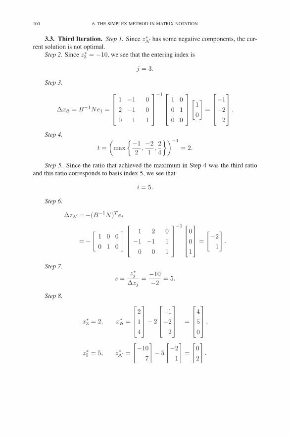
100 6. THE SIMPLEX METHOD IN MATRIX NOTATION
3.3. Third Iteration. Step 1. Since z∗N has some negative components, the cur-
rent solution is not optimal.
Step 2. Since z∗3 = −10, we see that the entering index is
j = 3.
Step 3.
∆xB = B−1Nej =
⎡
⎢
⎢
⎣
1 −1 0
2 −1 0
0 1 1
⎤
⎥
⎥
⎦
−1 ⎡
⎢
⎢
⎣
1 0
0 1
0 0
⎤
⎥
⎥
⎦
[
1
0
]
=
⎡
⎢
⎢
⎣
−1
−2
2
⎤
⎥
⎥
⎦
.
Step 4.
t =
(
max
{−1
2,−2
1,2
4
})−1
= 2.
Step 5. Since the ratio that achieved the maximum in Step 4 was the third ratio
and this ratio corresponds to basis index 5, we see that
i = 5.
Step 6.
∆zN =−(B−1N)T ei
=−[
1 0 0
0 1 0
]
⎡
⎢
⎢
⎣
1 2 0
−1 −1 1
0 0 1
⎤
⎥
⎥
⎦
−1 ⎡
⎢
⎢
⎣
0
0
1
⎤
⎥
⎥
⎦
=
[
−2
1
]
.
Step 7.
s =z∗j
∆zj=
−10
−2= 5.
Step 8.
x∗3 = 2, x∗
B =
⎡
⎢
⎢
⎣
2
1
4
⎤
⎥
⎥
⎦
− 2
⎡
⎢
⎢
⎣
−1
−2
2
⎤
⎥
⎥
⎦
=
⎡
⎢
⎢
⎣
4
5
0
⎤
⎥
⎥
⎦
,
z∗5 = 5, z∗N =
[
−10
7
]
− 5
[
−2
1
]
=
[
0
2
]
.
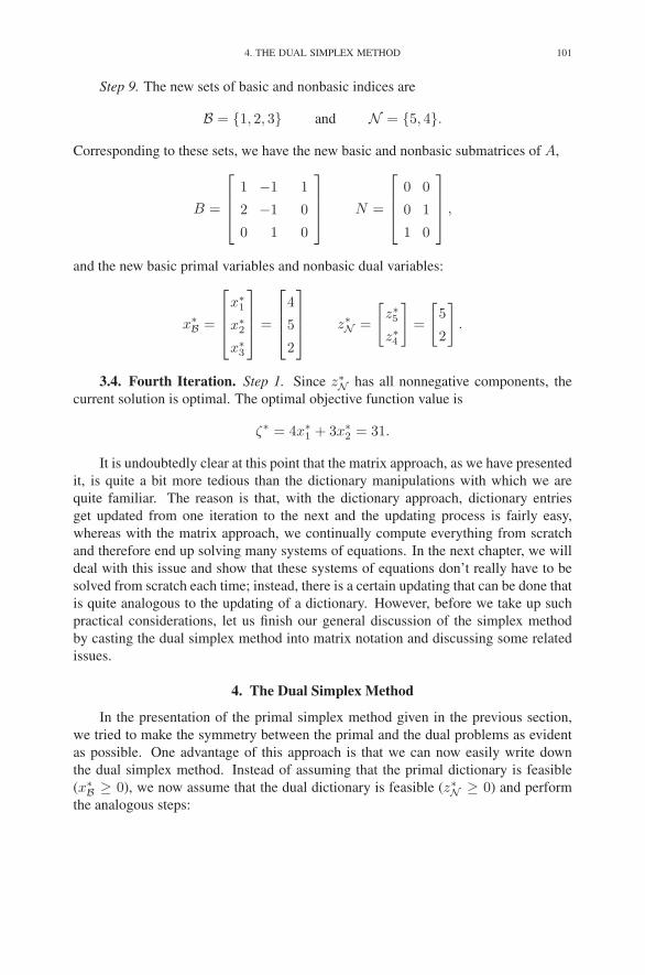
4. THE DUAL SIMPLEX METHOD 101
Step 9. The new sets of basic and nonbasic indices are
B = {1, 2, 3} and N = {5, 4}.
Corresponding to these sets, we have the new basic and nonbasic submatrices of A,
B =
⎡
⎢
⎢
⎣
1 −1 1
2 −1 0
0 1 0
⎤
⎥
⎥
⎦
N =
⎡
⎢
⎢
⎣
0 0
0 1
1 0
⎤
⎥
⎥
⎦
,
and the new basic primal variables and nonbasic dual variables:
x∗B =
⎡
⎢
⎢
⎣
x∗1
x∗2
x∗3
⎤
⎥
⎥
⎦
=
⎡
⎢
⎢
⎣
4
5
2
⎤
⎥
⎥
⎦
z∗N =
[
z∗5z∗4
]
=
[
5
2
]
.
3.4. Fourth Iteration. Step 1. Since z∗N has all nonnegative components, the
current solution is optimal. The optimal objective function value is
ζ∗ = 4x∗1 + 3x∗
2 = 31.
It is undoubtedly clear at this point that the matrix approach, as we have presented
it, is quite a bit more tedious than the dictionary manipulations with which we are
quite familiar. The reason is that, with the dictionary approach, dictionary entries
get updated from one iteration to the next and the updating process is fairly easy,
whereas with the matrix approach, we continually compute everything from scratch
and therefore end up solving many systems of equations. In the next chapter, we will
deal with this issue and show that these systems of equations don’t really have to be
solved from scratch each time; instead, there is a certain updating that can be done that
is quite analogous to the updating of a dictionary. However, before we take up such
practical considerations, let us finish our general discussion of the simplex method
by casting the dual simplex method into matrix notation and discussing some related
issues.
4. The Dual Simplex Method
In the presentation of the primal simplex method given in the previous section,
we tried to make the symmetry between the primal and the dual problems as evident
as possible. One advantage of this approach is that we can now easily write down
the dual simplex method. Instead of assuming that the primal dictionary is feasible
(x∗B ≥ 0), we now assume that the dual dictionary is feasible (z∗N ≥ 0) and perform
the analogous steps:

102 6. THE SIMPLEX METHOD IN MATRIX NOTATION
Step 1. Check for Optimality. If x∗B ≥ 0, stop. The current solution is opti-
mal. Note that for the dual simplex method, dual feasibility and complementarity are
maintained from the beginning, and the algorithm terminates once a primal feasible
solution is discovered.
Step 2. Select Entering Variable. Pick an index i ∈ B for which x∗i < 0. Variable
zi is the entering variable.
Step 3. Compute Dual Step Direction ∆zN . From the dual dictionary, we see that
∆zN = −(B−1N)T ei.
Step 4. Compute Dual Step Length. We wish to pick the largest s ≥ 0 for which
every component of zN remains nonnegative. As in the primal simplex method, this
computation involves computing the maximum of some ratios:
s =
(
maxj∈N
∆zj
z∗j
)−1
.
If s is not positive, then stop here—the dual is unbounded (implying, of course, that
the primal is infeasible).
Step 5. Select Leaving Variable. The leaving variable is chosen as any variable
zj , j ∈ N , for which the maximum in the calculation of s is obtained.
Step 6. Compute Primal Step Direction ∆xB. To see how x∗B changes in the dual
dictionary, it is convenient to look at the primal dictionary. Since in that dictionary xj
is the entering variable, we see that
∆xB = B−1Nej .
Step 7. Compute Primal Step Length. Since we know that xi is the leaving vari-
able in the primal dictionary, we see immediately that the step length for the primal
variables is
t =x∗
i
∆xi.
Step 8. Update Current Primal and Dual Solutions. We now have everything we
need to update the data in the dictionary:
x∗j ← t
x∗B ← x∗
B − t∆xB.
and
z∗i ← s
z∗N ← z∗N − s∆zN
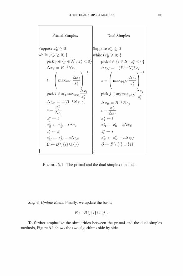
4. THE DUAL SIMPLEX METHOD 103
Primal Simplex
Suppose x∗B ≥ 0
while (z∗N �≥ 0) {pick j ∈ {j ∈ N : z∗j < 0}∆xB = B−1Nej
t =
⎛
⎜
⎝maxi∈B
∆xi
x∗i
⎞
⎟
⎠
−1
pick i ∈ argmaxi∈B∆xi
x∗i
∆zN = −(B−1N)T ei
s =z∗j
∆zj
x∗j ← t
x∗B ← x∗
B − t∆xB
z∗i ← s
z∗N ← z∗N − s∆zN
B ← B \ {i} ∪ {j}}
Dual Simplex
Suppose z∗N ≥ 0
while (x∗B �≥ 0) {
pick i ∈ {i ∈ B : x∗i < 0}
∆zN = −(B−1N)T ei
s =
⎛
⎜
⎝maxj∈N
∆zj
z∗j
⎞
⎟
⎠
−1
pick j ∈ argmaxj∈N∆zj
z∗j∆xB = B−1Nej
t =x∗
i
∆xi
x∗j ← t
x∗B ← x∗
B − t∆xB
z∗i ← s
z∗N ← z∗N − s∆zN
B ← B \ {i} ∪ {j}}
FIGURE 6.1. The primal and the dual simplex methods.
Step 9. Update Basis. Finally, we update the basis:
B ← B \ {i} ∪ {j}.
To further emphasize the similarities between the primal and the dual simplex
methods, Figure 6.1 shows the two algorithms side by side.
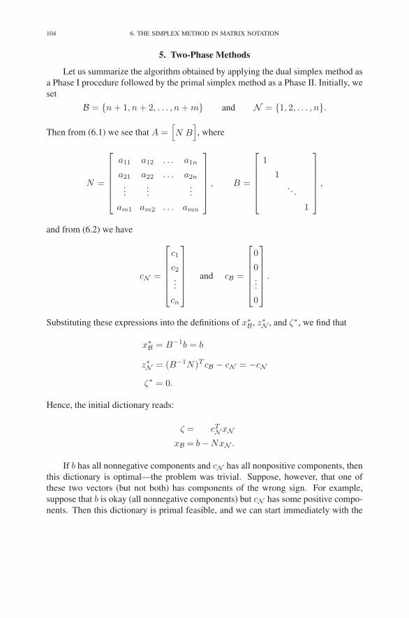
104 6. THE SIMPLEX METHOD IN MATRIX NOTATION
5. Two-Phase Methods
Let us summarize the algorithm obtained by applying the dual simplex method as
a Phase I procedure followed by the primal simplex method as a Phase II. Initially, we
set
B = {n + 1, n + 2, . . . , n + m} and N = {1, 2, . . . , n}.
Then from (6.1) we see that A =[
N B]
, where
N =
⎡
⎢
⎢
⎢
⎢
⎢
⎣
a11 a12 . . . a1n
a21 a22 . . . a2n
......
...
am1 am2 . . . amn
⎤
⎥
⎥
⎥
⎥
⎥
⎦
, B =
⎡
⎢
⎢
⎢
⎢
⎢
⎣
1
1
. . .
1
⎤
⎥
⎥
⎥
⎥
⎥
⎦
,
and from (6.2) we have
cN =
⎡
⎢
⎢
⎢
⎢
⎢
⎣
c1
c2
...
cn
⎤
⎥
⎥
⎥
⎥
⎥
⎦
and cB =
⎡
⎢
⎢
⎢
⎢
⎢
⎣
0
0...
0
⎤
⎥
⎥
⎥
⎥
⎥
⎦
.
Substituting these expressions into the definitions of x∗B, z∗N , and ζ∗, we find that
x∗B = B−1b = b
z∗N = (B−1N)T cB − cN = −cN
ζ∗ = 0.
Hence, the initial dictionary reads:
ζ = cTNxN
xB = b−NxN .
If b has all nonnegative components and cN has all nonpositive components, then
this dictionary is optimal—the problem was trivial. Suppose, however, that one of
these two vectors (but not both) has components of the wrong sign. For example,
suppose that b is okay (all nonnegative components) but cN has some positive compo-
nents. Then this dictionary is primal feasible, and we can start immediately with the
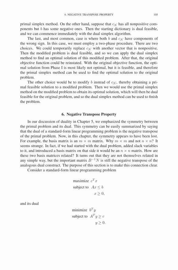
6. NEGATIVE TRANSPOSE PROPERTY 105
primal simplex method. On the other hand, suppose that cN has all nonpositive com-
ponents but b has some negative ones. Then the starting dictionary is dual feasible,
and we can commence immediately with the dual simplex algorithm.
The last, and most common, case is where both b and cN have components of
the wrong sign. In this case, we must employ a two-phase procedure. There are two
choices. We could temporarily replace cN with another vector that is nonpositive.
Then the modified problem is dual feasible, and so we can apply the dual simplex
method to find an optimal solution of this modified problem. After that, the original
objective function could be reinstated. With the original objective function, the opti-
mal solution from Phase I is most likely not optimal, but it is feasible, and therefore
the primal simplex method can be used to find the optimal solution to the original
problem.
The other choice would be to modify b instead of cN , thereby obtaining a pri-
mal feasible solution to a modified problem. Then we would use the primal simplex
method on the modified problem to obtain its optimal solution, which will then be dual
feasible for the original problem, and so the dual simplex method can be used to finish
the problem.
6. Negative Transpose Property
In our discussion of duality in Chapter 5, we emphasized the symmetry between
the primal problem and its dual. This symmetry can be easily summarized by saying
that the dual of a standard-form linear programming problem is the negative transpose
of the primal problem. Now, in this chapter, the symmetry appears to have been lost.
For example, the basis matrix is an m × m matrix. Why m × m and not n × n? It
seems strange. In fact, if we had started with the dual problem, added slack variables
to it, and introduced a basis matrix on that side it would be an n × n matrix. How are
these two basis matrices related? It turns out that they are not themselves related in
any simple way, but the important matrix B−1N is still the negative transpose of the
analogous dual construct. The purpose of this section is to make this connection clear.
Consider a standard-form linear programming problem
maximize cT x
subject to Ax≤ b
x≥ 0,
and its dual
minimize bT y
subject to AT y ≥ c
y ≥ 0.
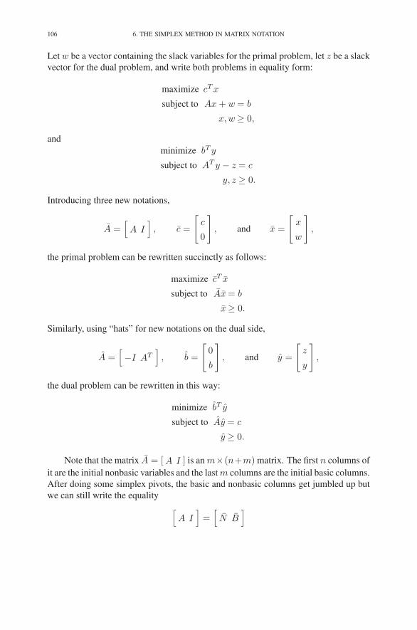
106 6. THE SIMPLEX METHOD IN MATRIX NOTATION
Let w be a vector containing the slack variables for the primal problem, let z be a slack
vector for the dual problem, and write both problems in equality form:
maximize cT x
subject to Ax + w = b
x, w ≥ 0,
and
minimize bT y
subject to AT y − z = c
y, z ≥ 0.
Introducing three new notations,
A =[
A I]
, c =
[
c
0
]
, and x =
[
x
w
]
,
the primal problem can be rewritten succinctly as follows:
maximize cT x
subject to Ax = b
x≥ 0.
Similarly, using “hats” for new notations on the dual side,
A =[
−I AT]
, b =
[
0
b
]
, and y =
[
z
y
]
,
the dual problem can be rewritten in this way:
minimize bT y
subject to Ay = c
y ≥ 0.
Note that the matrix A = [ A I ] is an m×(n+m) matrix. The first n columns of
it are the initial nonbasic variables and the last m columns are the initial basic columns.
After doing some simplex pivots, the basic and nonbasic columns get jumbled up but
we can still write the equality
[
A I]
=[
N B]
6. NEGATIVE TRANSPOSE PROPERTY 107
with the understanding that the equality only holds after rearranging the columns ap-
propriately.
On the dual side, the matrix A = [−I AT ] is an n × (n + m) matrix. The first
n columns of it are the initial basic variables (for the dual problem) and the last mcolumns are the initial nonbasic columns. If the same set of pivots that were applied
to the primal problem are also applied to the dual, then the columns get rearranged in
exactly the same way as they did for the primal and we can write
[
−I AT]
=[
B N]
again with the proviso that the columns of one matrix must be rearranged in a specific
manner to bring it into exact equality with the other matrix.
Now, the primal dictionary involves the matrix B−1N whereas the dual dictionary
involves the matrix B−1N . It probably doesn’t seem at all obvious that these two
matrices are negative transposes of each other. To see that it is so, consider what
happens when we multiply A by AT in both the permuted notation and the unpermuted
notation:
AAT =[
N B]
[
BT
NT
]
= NBT + BNT
and
AAT =[
A I]
[
−I
A
]
= −A + A = 0.
These two expressions obviously must agree so we see that
NBT + BNT = 0.
Putting the two terms on the opposite sides of the equality sign and multiplying on the
right by the inverse of BT and on the left by the inverse of B, we get that
B−1N = −(
B−1N)T
,
which is the property we wished to establish.

108 6. THE SIMPLEX METHOD IN MATRIX NOTATION
Exercises
6.1 Consider the following linear programming problem:
maximize −6x1 + 32x2 − 9x3
subject to −2x1 + 10x2 − 3x3 ≤−6
x1 − 7x2 + 2x3 ≤ 4
x1, x2, x3 ≥ 0.
Suppose that, in solving this problem, you have arrived at the following
dictionary:
ζ =−18− 3x4 + 2x2
x3 = 2− x4 + 4x2 − 2x5
x1 = 2x4 − x2 + 3x5.
(a) Which variables are basic? Which are nonbasic?
(b) Write down the vector, x∗B, of current primal basic solution values.
(c) Write down the vector, z∗N , of current dual nonbasic solution values.
(d) Write down B−1N .
(e) Is the primal solution associated with this dictionary feasible?
(f) Is it optimal?
(g) Is it degenerate?
6.2 Consider the following linear programming problem:
maximize x1 + 2x2 + 4x3 + 8x4 + 16x5
subject to x1 + 2x2 + 3x3 + 4x4 + 5x5 ≤ 2
7x1 + 5x2 − 3x3 − 2x4 ≤ 0
x1, x2, x3, x4, x5 ≥ 0.
Consider the situation in which x3 and x5 are basic and all other variables
are nonbasic. Write down:
(a) B,
(b) N ,
(c) b,
(d) cB,
(e) cN ,
(f) B−1N ,
(g) x∗B = B−1b,
(h) ζ∗ = cTBB−1b,
(i) z∗N = (B−1N)T cB − cN ,

NOTES 109
(j) the dictionary corresponding to this basis.
6.3 Solve the problem in Exercise 2.1 using the matrix form of the primal sim-
plex method.
6.4 Solve the problem in Exercise 2.4 using the matrix form of the dual simplex
method.
6.5 Solve the problem in Exercise 2.3 using the two-phase approach in matrix
form.
6.6 Find the dual of the following linear program:
maximize cT x
subject to a ≤ Ax ≤ b
l ≤ x ≤ u.
6.7 (a) Let A be a given m × n matrix, c a given n-vector, and b a given m-
vector. Consider the following max-min problem:
maxx≥0
miny≥0
(
cT x − yT Ax + bT y)
.
By noting that the inner optimization can be carried out explicitly, show
that this problem can be reduced to a linear programming problem.
Write it explicitly.
(b) What linear programming problem do you get if the min and max are
interchanged?
Notes
In this chapter, we have accomplished two tasks: (1) we have expressed the sim-
plex method in matrix notation, and (2) we have reduced the information we carry
from iteration to iteration to simply the list of basic variables together with current
values of the primal basic variables and the dual nonbasic variables. In particular, it is
not necessary to calculate explicitly all the entries of the matrix B−1N .
What’s in a name? There are times when one thing has two names. So far in this
book, we have discussed essentially only one algorithm: the simplex method (assum-
ing, of course, that specific pivot rules have been settled on). But this one algorithm is
sometimes referred to as the simplex method and at other times it is referred to as the
revised simplex method. The distinction being made with this new name has nothing to
do with the algorithm. Rather it refers to the specifics of an implementation. Indeed,
an implementation of the simplex method that avoids explicit calculation of the matrix
B−1N is referred to as an implementation of the revised simplex method. We shall
see in Chapter 8 why it is beneficial to avoid computing B−1N .


CHAPTER 7
Sensitivity and Parametric Analyses
In this chapter, we consider two related subjects. The first, called sensitivity anal-
ysis (or postoptimality analysis) addresses the following question: having found an
optimal solution to a given linear programming problem, how much can we change
the data and have the current partition into basic and nonbasic variables remain opti-
mal? The second subject addresses situations in which one wishes to solve not just one
linear program, but a whole family of problems parametrized by a single real variable.
We shall study parametric analysis in a very specific context in which we wish
to find the optimal solution to a given linear programming problem by starting from a
problem whose solution is trivially known and then deforming this problem back to the
original problem, maintaining as we go optimality of the current solution. The result
of this deformation approach to solving a linear programming problem is a new variant
of the simplex method, which is called the parametric self-dual simplex method. We
will see in later chapters that this variant of the simplex method resembles, in certain
respects, the interior-point methods that we shall study.
1. Sensitivity Analysis
One often needs to solve not just one linear programming problem but several
closely related problems. There are many reasons that this need might arise. For
example, the data that define the problem may have been rather uncertain and one
may wish to consider various possible data scenarios. Or perhaps the data are known
accurately but change from day to day, and the problem must be resolved for each new
day. Whatever the reason, this situation is quite common. So one is led to ask whether
it is possible to exploit the knowledge of a previously obtained optimal solution to
obtain more quickly the optimal solution to the problem at hand. Of course, the answer
is often yes, and this is the subject of this section.
We shall treat a number of possible situations. All of them assume that a problem
has been solved to optimality. This means that we have at our disposal the final,
optimal dictionary:
ζ = ζ∗ − z∗TN xN
xB = x∗B −B−1NxN .
111

112 7. SENSITIVITY AND PARAMETRIC ANALYSES
Suppose we wish to change the objective coefficients from c to, say, c. It is natural to
ask how the dictionary at hand could be adjusted to become a valid dictionary for the
new problem. That is, we want to maintain the current classification of the variables
into basic and nonbasic variables and simply adjust ζ∗, z∗N , and x∗B appropriately.
Recall from (6.7), (6.8), and (6.9) that
x∗B = B−1b,
z∗N = (B−1N)T cB − cN ,
ζ∗ = cTBB−1b.
Hence, the change from c to c requires us to recompute z∗N and ζ∗, but x∗B remains
unchanged. Therefore, after recomputing z∗N and ζ∗, the new dictionary is still primal
feasible, and so there is no need for a Phase I procedure: we can jump straight into the
primal simplex method, and if c is not too different from c, we can expect to get to the
new optimal solution in a relatively small number of steps.
Now suppose that instead of changing c, we wish to change only the right-hand
side b. In this case, we see that we need to recompute x∗B and ζ∗, but z∗N remains
unchanged. Hence, the new dictionary will be dual feasible, and so we can apply the
dual simplex method to arrive at the new optimal solution fairly directly.
Therefore, changing just the objective function or just the right-hand side results
in a new dictionary having nice feasibility properties. What if we need/want to change
some (or all) entries in both the objective function and the right-hand side and maybe
even the constraint matrix too? In this case, everything changes: ζ∗, z∗N , x∗B. Even
the entries in B and N change. Nonetheless, as long as the new basis matrix B is
nonsingular, we can make a new dictionary that preserves the old classification into
basic and nonbasic variables. The new dictionary will most likely be neither primal
feasible nor dual feasible, but if the changes in the data are fairly small in magnitude,
one would still expect that this starting dictionary will get us to an optimal solution
in fewer iterations than simply starting from scratch. While there is no guarantee
that any of these so-called warm-starts will end up in fewer iterations to optimality,
extensive empirical evidence indicates that this procedure often makes a substantial
improvement: sometimes the warm-started problems solve in as little as one percent
of the time it takes to solve the original problem.
1.1. Ranging. Often one does not wish to solve a modification of the original
problem, but instead just wants to ask a hypothetical question:
If I were to change the objective function by increasing or decreas-
ing one of the objective coefficients a small amount, how much
could I increase/decrease it without changing the optimality of my
current basis?
1. SENSITIVITY ANALYSIS 113
To study this question, let us suppose that c gets changed to c + t∆c, where t is a real
number and ∆c is a given vector (which is often all zeros except for a one in a single
entry, but we don’t need to restrict the discussion to this case). It is easy to see that z∗Ngets incremented by
t∆zN ,
where
(7.1) ∆zN = (B−1N)T ∆cB − ∆cN .
Hence, the current basis will remain dual feasible as long as
(7.2) z∗N + t∆zN ≥ 0.
We’ve manipulated this type of inequality many times before, and so it should be clear
that, for t > 0, this inequality will remain valid as long as
t ≤(
maxj∈N
−∆zj
z∗j
)−1
.
Similar manipulations show that, for t < 0, the lower bound is
t ≥(
minj∈N
−∆zj
z∗j
)−1
.
Combining these two inequalities, we see that t must lie in the interval
(
minj∈N
−∆zj
z∗j
)−1
≤ t ≤(
maxj∈N
−∆zj
z∗j
)−1
.
Let us illustrate these calculations with an example. Consider the following linear
programming problem:
maximize 5x1 + 4x2 + 3x3
subject to 2x1 + 3x2 + x3 ≤ 5
4x1 + x2 + 2x3 ≤ 11
3x1 + 4x2 + 2x3 ≤ 8
x1, x2, x3 ≥ 0 .

114 7. SENSITIVITY AND PARAMETRIC ANALYSES
The optimal dictionary for this problem is given by
ξ = 13− 3x2 − x4 − x6
x3 = 1 + x2 + 3x4 − 2x6
x1 = 2− 2x2 − 2x4 + x6
x5 = 1 + 5x2 + 2x4 .
The optimal basis is B = {3, 1, 5}. Suppose we want to know how much the coef-
ficient of 5 on x1 in the objective function can change without altering the optimality
of this basis. From the statement of the problem, we see that
c =[
5 4 3 0 0 0]T
.
Since we are interested in changes in the first coefficient, we put
∆c =[
1 0 0 0 0 0]T
.
We partition c according to the final (optimal) basis. Hence, we have
∆cB =
⎡
⎢
⎢
⎣
0
1
0
⎤
⎥
⎥
⎦
and ∆cN =
⎡
⎢
⎢
⎣
0
0
0
⎤
⎥
⎥
⎦
.
Next, we need to compute ∆zN using (7.1). We could compute B−1N from scratch,
but it is easier to extract it from the constraint coefficients in the final dictionary. In-
deed,
−B−1N =
⎡
⎢
⎢
⎣
1 3−2
−2−2 1
5 2 0
⎤
⎥
⎥
⎦
.
Hence, from (7.1) we see that
∆zN =
⎡
⎢
⎢
⎣
2
2
−1
⎤
⎥
⎥
⎦
.
Now, (7.2) gives the condition on t. Writing it out componentwise, we get
3 + 2t ≥ 0, 1 + 2t ≥ 0, and 1 − t ≥ 0.
2. PARAMETRIC ANALYSIS AND THE HOMOTOPY METHOD 115
These three inequalities, which must all hold, can be summarized by saying that
−1
2≤ t ≤ 1
Hence, in terms of the coefficient on x1, we finally see that it can range from 4.5 to 6.
Now suppose we change b to b + t∆b and ask how much t can change before
the current basis becomes nonoptimal. In this case, z∗N does not change, but x∗B gets
incremented by t∆xB, where
∆xB = B−1∆b.
Hence, the current basis will remain optimal as long as t lies in the interval
(
mini∈B
−∆xi
x∗i
)−1
≤ t ≤(
maxi∈B
−∆xi
x∗i
)−1
.
2. Parametric Analysis and the Homotopy Method
In this section, we illustrate the notion of parametric analysis by applying a tech-
nique called the homotopy method to get a new algorithm for solving linear program-
ming problems. The homotopy method is a general technique in which one creates a
continuous deformation that changes a given difficult problem into a related but triv-
ially solved problem and then attempts to work backwards from the trivial problem to
the difficult problem by solving (hopefully without too much effort) all the problems
in between. Of course, there is a continuum of problems between the hard one and the
trivial one, and so we shouldn’t expect that this technique will be effective in every
situation; but for linear programming and for many other problem domains, it turns
out to yield efficient algorithms.
We start with an example. Suppose we wish to solve the following linear pro-
gramming problem:
maximize −2x1 + 3x2
subject to −x1 + x2 ≤−1
−x1 − 2x2 ≤−2
x2 ≤ 1
x1, x2 ≥ 0.

116 7. SENSITIVITY AND PARAMETRIC ANALYSES
The starting dictionary is
ζ = − 2x1 − (−3)x2
x3 =−1 + x1 − x2
x4 =−2 + x1 + 2x2
x5 = 1 − x2 .
This dictionary is neither primal nor dual feasible. Let’s perturb it by adding a positive
real number μ to each right-hand side and subtracting it from each objective function
coefficient. We now arrive at a family of dictionaries, parametrized by μ:
(7.3)
ζ = − (2 + μ)x1 − (−3 + μ)x2
x3 =−1 + μ + x1 − x2
x4 =−2 + μ + x1 + 2x2
x5 = 1 + μ − x2 .
Clearly, for μ sufficiently large, specifically μ ≥ 3, this dictionary is both primal
and dual feasible. Hence, the associated solution x = [0, 0,−1 + μ,−2 + μ, 1 + μ]is optimal. Starting with μ large, we reduce it as much as we can while keeping
dictionary (7.3) optimal. This dictionary will become nonoptimal as soon as μ < 3,
since the associated dual variable y∗2 = −3 + μ will become negative. In other words,
the coefficient of x2, which is 3− μ, will become positive. This change of sign on the
coefficient of x2 suggests that we make a primal pivot in which x2 enters the basis.
The usual ratio test (using the specific value of μ = 3) indicates that x3 must be the
leaving variable. Making the pivot, we get
ζ =−3 + 4μ− μ2 − (−1 + 2μ)x1 − (3 − μ)x3
x2 =−1 + μ + x1 − x3
x4 =−4 + 3μ + 3x1 − 2x3
x5 = 2 + x1 + x3 .
This dictionary is optimal as long as
−1 + 2μ ≥ 0, 3 − μ ≥ 0,
−1 + μ ≥ 0, −4 + 3μ ≥ 0.
These inequalities reduce to4
3≤ μ ≤ 3.
2. PARAMETRIC ANALYSIS AND THE HOMOTOPY METHOD 117
So now we can reduce μ from its current value of 3 down to 4/3. If we reduce it
below 4/3, the primal feasibility inequality, −4 + 3μ ≥ 0, becomes violated. This
violation suggests that we perform a dual pivot with x4 serving as the leaving variable.
The usual (dual) ratio test (with μ = 4/3) then tells us that x1 must be the entering
variable. Doing the pivot, we get
ζ =− 53 + 1
3μ + μ2 − (− 13 + 2
3μ)x4 − ( 73 + 1
3μ)x3
x2 = 13 + 1
3x4 − 13x3
x1 = 43 − μ + 1
3x4 + 23x3
x5 = 23 + μ − 1
3x4 + 13x3 .
Now the conditions for optimality are
−1
3+
2
3μ ≥ 0,
7
3+
1
3μ ≥ 0,
4
3− μ ≥ 0,
2
3+ μ ≥ 0,
which reduce to1
2≤ μ ≤ 4
3.
For the next iteration, we reduce μ to 1/2 and see that the inequality that becomes
binding is the dual feasibility inequality
−1
3+
2
3μ ≥ 0.
Hence, we do a primal pivot with x4 entering the basis. The leaving variable is x5,
and the new dictionary is
ζ =−1 − μ2 − (1 − 2μ)x5 − (2 + μ)x3
x2 = 1 + μ − x5
x1 = 2 − x5 + x3
x4 = 2 + 3μ − 3x5 + x3 .
For this dictionary, the range of optimality is given by
1 − 2μ ≥ 0, 2 + μ ≥ 0,
1 + μ ≥ 0, 2 + 3μ ≥ 0,

118 7. SENSITIVITY AND PARAMETRIC ANALYSES
which reduces to
−2
3≤ μ ≤ 1
2.
This range covers μ = 0, and so now we can set μ to 0 and get an optimal dictionary
for our original problem:
ζ =−1− x5 − 2x3
x2 = 1− x5
x1 = 2− x5 + x3
x4 = 2− 3x5 + x3 .
The algorithm we have just illustrated is called the parametric self-dual simplex
method.1 We shall often refer to it more simply as the self-dual simplex method. It
has some attractive features. First, in contrast to the methods presented earlier, this
algorithm does not require a separate Phase I procedure. It starts with any problem,
be it primal infeasible, dual infeasible, or both, and it systematically performs pivots
(whether primal or dual) until it finds an optimal solution.
A second feature is that a trivial modification of the algorithm can avoid en-
tirely ever encountering a degenerate dictionary. Indeed, suppose that, instead of
adding/subtracting μ from each of the right-hand sides and objective coefficients, we
add/subtract a positive constant times μ. Suppose further that the positive constant
is different in each addition/subtraction. In fact, suppose that they are chosen inde-
pendently from, say, a uniform distribution on [1/2, 3/2]. Then with probability one,
the algorithm will produce no primal degenerate or dual degenerate dictionary in any
iteration. In Chapter 3, we discussed perturbing the right-hand side of a linear pro-
gramming problem to avoid degeneracy in the primal simplex method, but back then
the perturbation changed the problem. The present perturbation does not in any way
affect the problem that is solved.
With the above randomization trick to resolve the degeneracy issue, the analysis of
the convergence of the algorithm is straightforward. Indeed, let us consider a problem
that is feasible and bounded (the questions regarding feasibility and boundedness are
addressed in Exercise 7.10). For each nondegenerate pivot, the next value of μ will
be strictly less than the current value. Since each of these μ values is determined by a
partition of the variables into basics and nonbasics and there are only a finite number
of such partitions, it follows that the method must reach a partition with a negative μvalue in a finite number of steps.
1In the first edition, this method was called the primal–dual simplex method.
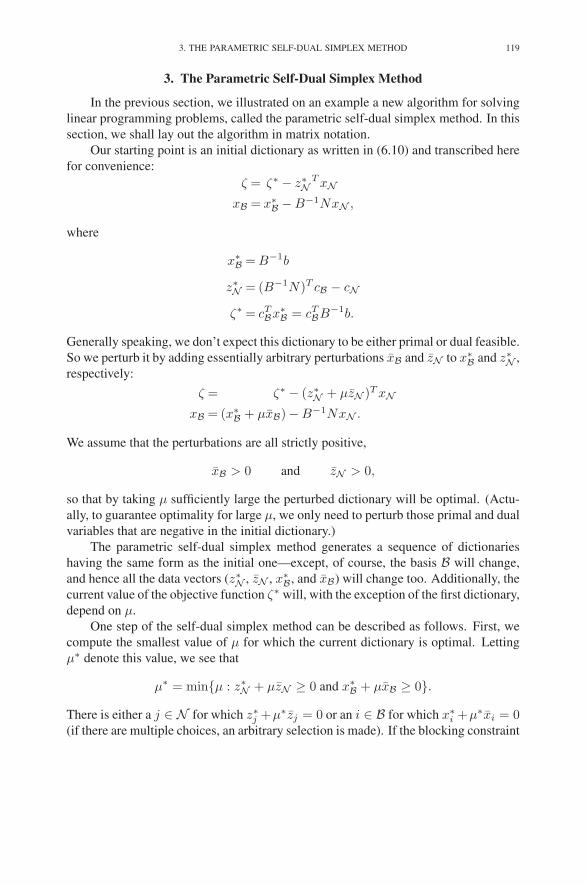
3. THE PARAMETRIC SELF-DUAL SIMPLEX METHOD 119
3. The Parametric Self-Dual Simplex Method
In the previous section, we illustrated on an example a new algorithm for solving
linear programming problems, called the parametric self-dual simplex method. In this
section, we shall lay out the algorithm in matrix notation.
Our starting point is an initial dictionary as written in (6.10) and transcribed here
for convenience:
ζ = ζ∗ − z∗NT xN
xB = x∗B −B−1NxN ,
where
x∗B = B−1b
z∗N = (B−1N)T cB − cN
ζ∗ = cTBx∗
B = cTBB−1b.
Generally speaking, we don’t expect this dictionary to be either primal or dual feasible.
So we perturb it by adding essentially arbitrary perturbations xB and zN to x∗B and z∗N ,
respectively:
ζ = ζ∗ − (z∗N + μzN )T xN
xB = (x∗B + μxB)−B−1NxN .
We assume that the perturbations are all strictly positive,
xB > 0 and zN > 0,
so that by taking μ sufficiently large the perturbed dictionary will be optimal. (Actu-
ally, to guarantee optimality for large μ, we only need to perturb those primal and dual
variables that are negative in the initial dictionary.)
The parametric self-dual simplex method generates a sequence of dictionaries
having the same form as the initial one—except, of course, the basis B will change,
and hence all the data vectors (z∗N , zN , x∗B, and xB) will change too. Additionally, the
current value of the objective function ζ∗ will, with the exception of the first dictionary,
depend on μ.
One step of the self-dual simplex method can be described as follows. First, we
compute the smallest value of μ for which the current dictionary is optimal. Letting
μ∗ denote this value, we see that
μ∗ = min{μ : z∗N + μzN ≥ 0 and x∗B + μxB ≥ 0}.
There is either a j ∈ N for which z∗j +μ∗zj = 0 or an i ∈ B for which x∗i +μ∗xi = 0
(if there are multiple choices, an arbitrary selection is made). If the blocking constraint
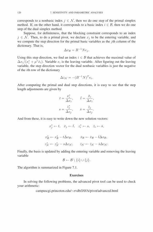
120 7. SENSITIVITY AND PARAMETRIC ANALYSES
corresponds to a nonbasic index j ∈ N , then we do one step of the primal simplex
method. If, on the other hand, it corresponds to a basic index i ∈ B, then we do one
step of the dual simplex method.
Suppose, for definiteness, that the blocking constraint corresponds to an index
j ∈ N . Then, to do a primal pivot, we declare xj to be the entering variable, and
we compute the step direction for the primal basic variables as the jth column of the
dictionary. That is,
∆xB = B−1Nej .
Using this step direction, we find an index i ∈ B that achieves the maximal value of
∆xi/(x∗i + μ∗xi). Variable xi is the leaving variable. After figuring out the leaving
variable, the step direction vector for the dual nonbasic variables is just the negative
of the ith row of the dictionary
∆zN = −(B−1N)T ei.
After computing the primal and dual step directions, it is easy to see that the step
length adjustments are given by
t =x∗
i
∆xi, t =
xi
∆xi,
s =z∗j
∆zj, s =
zj
∆zj.
And from these, it is easy to write down the new solution vectors:
x∗j ← t, xj ← t, z∗i ← s, zi ← s,
x∗B ← x∗
B − t∆xB, xB ← xB − t∆xB,
z∗N ← z∗N − s∆zN , zN ← zN − s∆zN .
Finally, the basis is updated by adding the entering variable and removing the leaving
variable
B ← B \ {i} ∪ {j}.
The algorithm is summarized in Figure 7.1.
Exercises
In solving the following problems, the advanced pivot tool can be used to check
your arithmetic:
campuscgi.princeton.edu/∼rvdb/JAVA/pivot/advanced.html
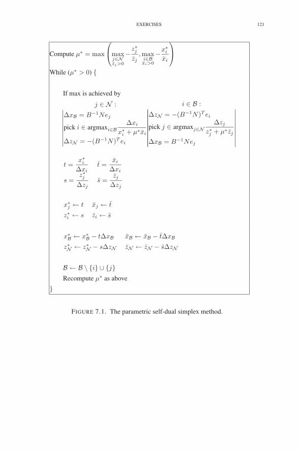
EXERCISES 121
Compute μ∗ = max
⎛
⎝maxj∈Nzj>0
−z∗jzj
,maxi∈Bxi>0
−x∗i
xi
⎞
⎠
While (μ∗ > 0) {
If max is achieved by
j ∈ N :
∆xB = B−1Nej
pick i ∈ argmaxi∈B∆xi
x∗i + μ∗xi
∆zN = −(B−1N)T ei
i ∈ B :
∆zN = −(B−1N)T ei
pick j ∈ argmaxj∈N∆zj
z∗j + μ∗zj
∆xB = B−1Nej
t =x∗
i
∆xit =
xi
∆xi
s =z∗j
∆zjs =
zj
∆zj
x∗j ← t xj ← t
z∗i ← s zi ← s
x∗B ← x∗
B − t∆xB xB ← xB − t∆xB
z∗N ← z∗N − s∆zN zN ← zN − s∆zN
B ← B \ {i} ∪ {j}Recompute μ∗ as above
}
FIGURE 7.1. The parametric self-dual simplex method.
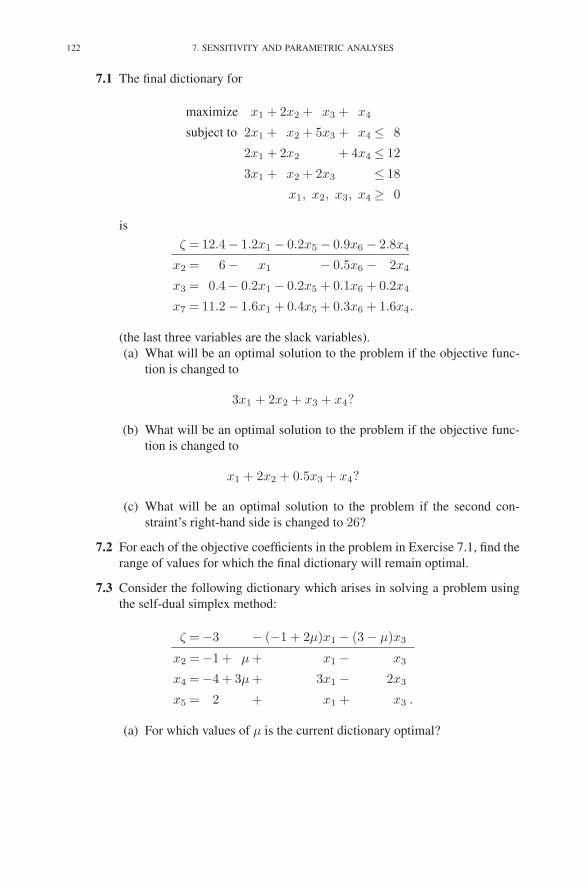
122 7. SENSITIVITY AND PARAMETRIC ANALYSES
7.1 The final dictionary for
maximize x1 + 2x2 + x3 + x4
subject to 2x1 + x2 + 5x3 + x4 ≤ 8
2x1 + 2x2 + 4x4 ≤ 12
3x1 + x2 + 2x3 ≤ 18
x1, x2, x3, x4 ≥ 0
is
ζ = 12.4− 1.2x1 − 0.2x5 − 0.9x6 − 2.8x4
x2 = 6− x1 − 0.5x6 − 2x4
x3 = 0.4− 0.2x1 − 0.2x5 + 0.1x6 + 0.2x4
x7 = 11.2− 1.6x1 + 0.4x5 + 0.3x6 + 1.6x4.
(the last three variables are the slack variables).
(a) What will be an optimal solution to the problem if the objective func-
tion is changed to
3x1 + 2x2 + x3 + x4?
(b) What will be an optimal solution to the problem if the objective func-
tion is changed to
x1 + 2x2 + 0.5x3 + x4?
(c) What will be an optimal solution to the problem if the second con-
straint’s right-hand side is changed to 26?
7.2 For each of the objective coefficients in the problem in Exercise 7.1, find the
range of values for which the final dictionary will remain optimal.
7.3 Consider the following dictionary which arises in solving a problem using
the self-dual simplex method:
ζ =−3 − (−1 + 2μ)x1 − (3 − μ)x3
x2 =−1 + μ + x1 − x3
x4 =−4 + 3μ + 3x1 − 2x3
x5 = 2 + x1 + x3 .
(a) For which values of μ is the current dictionary optimal?
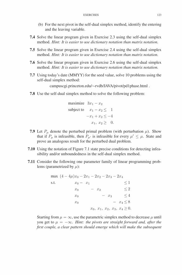
EXERCISES 123
(b) For the next pivot in the self-dual simplex method, identify the entering
and the leaving variable.
7.4 Solve the linear program given in Exercise 2.3 using the self-dual simplex
method. Hint: It is easier to use dictionary notation than matrix notation.
7.5 Solve the linear program given in Exercise 2.4 using the self-dual simplex
method. Hint: It is easier to use dictionary notation than matrix notation.
7.6 Solve the linear program given in Exercise 2.6 using the self-dual simplex
method. Hint: It is easier to use dictionary notation than matrix notation.
7.7 Using today’s date (MMYY) for the seed value, solve 10 problems using the
self-dual simplex method:
campuscgi.princeton.edu/∼rvdb/JAVA/pivot/pd1phase.html .
7.8 Use the self-dual simplex method to solve the following problem:
maximize 3x1 − x2
subject to x1 − x2 ≤ 1
−x1 + x2 ≤−4
x1, x2 ≥ 0.
7.9 Let Pμ denote the perturbed primal problem (with perturbation μ). Show
that if Pμ is infeasible, then Pμ′ is infeasible for every μ′ ≤ μ. State and
prove an analogous result for the perturbed dual problem.
7.10 Using the notation of Figure 7.1 state precise conditions for detecting infea-
sibility and/or unboundedness in the self-dual simplex method.
7.11 Consider the following one parameter family of linear programming prob-
lems (parametrized by μ):
max (4 − 4μ)x0 − 2x1 − 2x2 − 2x3 − 2x4
s.t. x0 − x1 ≤ 1
x0 − x2 ≤ 2
x0 − x3 ≤ 4
x0 − x4 ≤ 8
x0, x1, x2, x3, x4 ≥ 0.
Starting from μ = ∞, use the parametric simplex method to decrease μ until
you get to μ = −∞. Hint: the pivots are straight forward and, after the
first couple, a clear pattern should emerge which will make the subsequent

124 7. SENSITIVITY AND PARAMETRIC ANALYSES
pivots easy. Clearly indicate the range of μ values for which each dictionary
is optimal.
Notes
Parametric analysis has its roots in Gass & Saaty (1955). G.B. Dantzig’s clas-
sic book (Dantzig 1963) describes the self-dual simplex method under the name of
the self-dual parametric simplex method. It is a special case of “Lemke’s algorithm”
for the linear complementarity problem (Lemke 1965) (see Exercise 18.7). Smale
(1983) and Borgwardt (1982) were first to realize that the parametric self-dual sim-
plex method is amenable to probabilistic analysis. For a more recent discussion of
homotopy methods and the parametric self-dual simplex method, see Nazareth (1986)
and Nazareth (1987).

CHAPTER 8
Implementation Issues
In the previous chapter, we rewrote the simplex method using matrix notation.
This is the first step toward our aim of describing the simplex method as one would
implement it as a computer program. In this chapter, we shall continue in this direction
by addressing some important implementation issues.
The most time-consuming steps in the simplex method are the computations
∆xB = B−1Nej and ∆zN = −(B−1N)T ei,
and the difficulty in these steps arises from the B−1. Of course, we don’t ever actually
compute the inverse of the basis matrix. Instead, we calculate, say, ∆xB by solving
the following system of equations:
(8.1) B∆xB = aj ,
where
aj = Nej
is the column of N associated with nonbasic variable xj .
Similarly, the calculation of ∆zN is also broken into two steps:
BT v = ei,(8.2)
∆zN =−NT v.
Here, the first step is the solution of a large system of equations, this time involving
BT instead of B, and the second step is the comparatively trivial task of multiplying
a vector on the left by the matrix −NT .
Solving the systems of equations (8.1) and (8.2) is where most of the complexity
of a simplex iteration lies. We discuss solving such systems in the first two sections.
In the second section, we look at the effect of sparsity on these systems. The next
few sections explain how to reuse and/or update the computations of one iteration in
subsequent iterations. In the final sections, we address a few other issues that affect
the efficiency of an implementation.
125

126 8. IMPLEMENTATION ISSUES
1. Solving Systems of Equations: LU -Factorization
In this section, we discuss solving systems of equations of the form
Bx = b,
where B is an invertible m × m matrix and b is an arbitrary m-vector. (Analysis of
the transpose BT x = b is left to Exercise 8.4.) Our first thought is to use Gaussian
elimination. This idea is correct, but to explain how Gaussian elimination is actually
implemented, we need to take a fresh look at how it works. To explain, let us consider
an example:
B =
⎡
⎢
⎢
⎢
⎢
⎢
⎢
⎢
⎣
2 4 −2
3 1 1
−1 −1 −2
−1 −6
1 4
⎤
⎥
⎥
⎥
⎥
⎥
⎥
⎥
⎦
.
(Note that, to emphasize the importance of sparsity, zero entries are simply left blank.)
In Gaussian elimination, one begins by subtracting appropriate multiples of the first
row from each subsequent row to get zeros in the first column below the diagonal. For
our specific example, we subtract 3/2 times the first row from the second row and we
subtract −1/2 times the first row from the third row. The result is
⎡
⎢
⎢
⎢
⎢
⎢
⎢
⎢
⎣
2 4 −2
1 −6 1 3
1 −3
−1 −6
1 4
⎤
⎥
⎥
⎥
⎥
⎥
⎥
⎥
⎦
.
Shortly, we will want to remember the values of the nonzero elements in the first
column. Therefore, let us agree to do the row operations that are required to eliminate
nonzeros, but when we write down the result of the elimination, we will leave the
nonzeros there. With this convention, the result of the elimination of the first column
can be written as⎡
⎢
⎢
⎢
⎢
⎢
⎢
⎢
⎣
2 4 −2
3 1 −6 1 3
−1 1 −3
−1 −6
1 4
⎤
⎥
⎥
⎥
⎥
⎥
⎥
⎥
⎦
.

1. SOLVING SYSTEMS OF EQUATIONS: LU -FACTORIZATION 127
Note that we have drawn a line to separate the eliminated top/left parts of the matrix
from the uneliminated lower-right part.
Next, we eliminate the nonzeros below the second diagonal (there’s only one)
by subtracting an appropriate multiple of the second row from each subsequent row.
Again, we write the answer without zeroing out the eliminated elements:
⎡
⎢
⎢
⎢
⎢
⎢
⎢
⎢
⎣
2 4 −2
3 1 −6 1 3
−1 1 −3
−1 −6 1 −3
1 4
⎤
⎥
⎥
⎥
⎥
⎥
⎥
⎥
⎦
.
After eliminating the third column, we get
⎡
⎢
⎢
⎢
⎢
⎢
⎢
⎢
⎣
2 4 −2
3 1 −6 1 3
−1 1 −3
−1 −6 1 −21
1 7
⎤
⎥
⎥
⎥
⎥
⎥
⎥
⎥
⎦
.
Now, the remaining uneliminated part is already an upper triangular matrix, and hence
no more elimination is required.
At this point, you are probably wondering how this strangely produced matrix is
related to the original matrix B. The answer is both simple and elegant. First, take
the final matrix and split it into three matrices: the matrix consisting of all elements
on or below the diagonal, the matrix consisting of just the diagonal elements, and the
matrix consisting of all elements on or above the diagonal. It is amazing but true that
B is simply the product of the resulting lower triangular matrix times the inverse of
the diagonal matrix times the upper triangular matrix:
B =
⎡
⎢
⎢
⎢
⎢
⎢
⎢
⎢
⎣
2
3 1
−1 1
−1 −6 1
1 7
⎤
⎥
⎥
⎥
⎥
⎥
⎥
⎥
⎦
⎡
⎢
⎢
⎢
⎢
⎢
⎢
⎢
⎣
2
1
1
1
7
⎤
⎥
⎥
⎥
⎥
⎥
⎥
⎥
⎦
−1 ⎡
⎢
⎢
⎢
⎢
⎢
⎢
⎢
⎣
2 4 −2
1 −6 1 3
1 −3
1 −21
7
⎤
⎥
⎥
⎥
⎥
⎥
⎥
⎥
⎦
.

128 8. IMPLEMENTATION ISSUES
(If you don’t believe it, multiply them and see.) Normally, the product of the lower
triangular matrix and the diagonal matrix is denoted by L,
L =
⎡
⎢
⎢
⎢
⎢
⎢
⎢
⎢
⎣
2
3 1
−1 1
−1 −6 1
1 7
⎤
⎥
⎥
⎥
⎥
⎥
⎥
⎥
⎦
⎡
⎢
⎢
⎢
⎢
⎢
⎢
⎢
⎣
2
1
1
1
7
⎤
⎥
⎥
⎥
⎥
⎥
⎥
⎥
⎦
−1
=
⎡
⎢
⎢
⎢
⎢
⎢
⎢
⎢
⎣
132 1
− 12 1
−1 −6 1
1 1
⎤
⎥
⎥
⎥
⎥
⎥
⎥
⎥
⎦
,
and the upper triangular matrix is denote by U :
U =
⎡
⎢
⎢
⎢
⎢
⎢
⎢
⎢
⎣
2 4 −2
1 −6 1 3
1 −3
1 −21
7
⎤
⎥
⎥
⎥
⎥
⎥
⎥
⎥
⎦
.
The resulting representation,
B = LU,
is called an LU -factorization of B. Finding an LU -factorization is equivalent to
Gaussian elimination in the sense that multiplying B on the left by L−1 has the effect
of applying row operations to B to put it into upper-triangular form U .
The value of an LU -factorization is that it can be used to solve systems of equa-
tions. For example, suppose that we wish to solve equation (8.1), where B is as above
and
(8.3) aj =
⎡
⎢
⎢
⎢
⎢
⎢
⎢
⎢
⎣
7
−2
0
3
0
⎤
⎥
⎥
⎥
⎥
⎥
⎥
⎥
⎦
.
First, we substitute LU for B so that the system becomes
LU∆xB = aj .
Now, if we let y = U∆xB, then we can solve
Ly = b

1. SOLVING SYSTEMS OF EQUATIONS: LU -FACTORIZATION 129
for y, and once y is known, we can solve
U∆xB = y
for ∆xB. Because L is lower triangular, solving Ly = b is easy. Indeed, writing the
system out,⎡
⎢
⎢
⎢
⎢
⎢
⎢
⎢
⎣
132 1
− 12 1
−1 −6 1
1 1
⎤
⎥
⎥
⎥
⎥
⎥
⎥
⎥
⎦
⎡
⎢
⎢
⎢
⎢
⎢
⎢
⎢
⎣
y1
y2
y3
y4
y5
⎤
⎥
⎥
⎥
⎥
⎥
⎥
⎥
⎦
=
⎡
⎢
⎢
⎢
⎢
⎢
⎢
⎢
⎣
7
−2
0
3
0
⎤
⎥
⎥
⎥
⎥
⎥
⎥
⎥
⎦
,
we notice immediately that y1 = 7. Then, given y1, it becomes clear from the second
equation that y2 = −2 − (3/2)y1 = −25/2. Continuing in this way, we find that
⎡
⎢
⎢
⎢
⎢
⎢
⎢
⎢
⎣
y1
y2
y3
y4
y5
⎤
⎥
⎥
⎥
⎥
⎥
⎥
⎥
⎦
=
⎡
⎢
⎢
⎢
⎢
⎢
⎢
⎢
⎣
7
− 252
72232
− 72
⎤
⎥
⎥
⎥
⎥
⎥
⎥
⎥
⎦
.
The process of successively solving for the elements of the vector y starting with the
first and proceeding to the last is called forward substitution.
Of course, solving U∆xB = y is easy too, since U is upper triangular. The system
to solve is given by
⎡
⎢
⎢
⎢
⎢
⎢
⎢
⎢
⎣
2 4 −2
1 −6 1 3
1 −3
1 −21
7
⎤
⎥
⎥
⎥
⎥
⎥
⎥
⎥
⎦
⎡
⎢
⎢
⎢
⎢
⎢
⎢
⎢
⎣
∆x1
∆x2
∆x3
∆x4
∆x5
⎤
⎥
⎥
⎥
⎥
⎥
⎥
⎥
⎦
=
⎡
⎢
⎢
⎢
⎢
⎢
⎢
⎢
⎣
7
− 252
72232
− 72
⎤
⎥
⎥
⎥
⎥
⎥
⎥
⎥
⎦
(note that, to keep notations simple, we are assuming that the basic indices are 1through 5 so that ∆xB = (∆x1,∆x2,∆x3,∆x4,∆x5)). This time we start with the
last equation and see that ∆x5 = −1/2. Then the second to last equation tells us that

130 8. IMPLEMENTATION ISSUES
∆x4 = 23/2 + 21(∆x5) = 1. After working our way to the first equation, we have
∆xB =
⎡
⎢
⎢
⎢
⎢
⎢
⎢
⎢
⎣
∆x1
∆x2
∆x3
∆x4
∆x5
⎤
⎥
⎥
⎥
⎥
⎥
⎥
⎥
⎦
=
⎡
⎢
⎢
⎢
⎢
⎢
⎢
⎢
⎣
−1
0
2
1
− 12
⎤
⎥
⎥
⎥
⎥
⎥
⎥
⎥
⎦
.
This process of working from the last element of ∆xB back to the first is called back-
ward substitution.
2. Exploiting Sparsity
In the previous section, we took a specific matrix B and constructed an LU fac-
torization of it. However, with that example we were lucky in that every diagonal
element was nonzero at the moment it was used to eliminate the nonzeros below it.
Had we encountered a zero diagonal element, we would have been forced to rearrange
the columns and/or the rows of the matrix to put a nonzero element in this position.
For a random matrix (whatever that means), the odds of encountering a zero are nil,
but a basis matrix can be expected to have plenty of zeros in it, since, for example, it
is likely to contain columns associated with slack variables, which are all zero except
for one 1. A matrix that contains zeros is called a sparse matrix.
When a sparse matrix has lots of zeros, two things happen. First, the chances
of being required to make row and/or column permutations is high. Second, addi-
tional computational efficiency can be obtained by making further row and/or column
permutations with the aim of keeping L and/or U as sparse as possible.
The problem of finding the “best” permutation is, in itself, harder than the linear
programming problem that we ultimately wish to solve. But there are simple heuristics
that help to preserve sparsity in L and U . We shall focus on just one such heuristic,
called the minimum-degree ordering heuristic, which is describe as follows:
Before eliminating the nonzeros below a diagonal “pivot” ele-
ment, scan all uneliminated rows and select the sparsest row, i.e.,
that row having the fewest nonzeros in its uneliminated part (ties
can be broken arbitrarily). Swap this row with the pivot row. Then
scan the uneliminated nonzeros in this row and select that one
whose column has the fewest nonzeros in its uneliminated part.
Swap this column with the pivot column so that this nonzero be-
comes the pivot element. (Of course, provisions should be made
to reject such a pivot element if its value is close to zero.)
As a matter of terminology, the number of nonzeros in the uneliminated part of a
row/column is called the degree of the row/column. Hence, the name of the heuristic.

2. EXPLOITING SPARSITY 131
Let’s apply the minimum-degree heuristic to the LU -factorization of the matrix
B studied in the previous section. To keep track of the row and column permutations,
we will indicate original row indices on the left and original column indices across the
top. Hence, we start with:
B =
1 2 3 4 5
1
2
3
4
5
⎡
⎢
⎢
⎢
⎢
⎢
⎢
⎢
⎣
2 4 −2
3 1 1
−1 −1 −2
−1 −6
1 4
⎤
⎥
⎥
⎥
⎥
⎥
⎥
⎥
⎦
.
To begin, row 4 has the fewest nonzeros, and within row 4, the −1 in column 2 belongs
to the column with the fewest nonzeros. Hence, we swap rows 1 and 4 and we swap
columns 1 and 2 to rewrite B as
B =
2 1 3 4 5
4
2
3
1
5
⎡
⎢
⎢
⎢
⎢
⎢
⎢
⎢
⎣
−1 −6
1 3 1
−1 −1 −2
2 4 −2
1 4
⎤
⎥
⎥
⎥
⎥
⎥
⎥
⎥
⎦
.
Now, we eliminate the nonzeros under the first diagonal element (and, as before, we
leave the eliminated nonzeros as they were). The result is
2 1 3 4 5
4
2
3
1
5
⎡
⎢
⎢
⎢
⎢
⎢
⎢
⎢
⎣
−1 −6
1 3 1 −6
−1 −1 −2
2 4 −2
1 4
⎤
⎥
⎥
⎥
⎥
⎥
⎥
⎥
⎦
.
Before doing the elimination associated with the second diagonal element, we
note that row 5 is the row with minimum degree, and within row 5, the element 1 in
column 3 has minimum column degree. Hence, we swap rows 2 and 5 and we swap
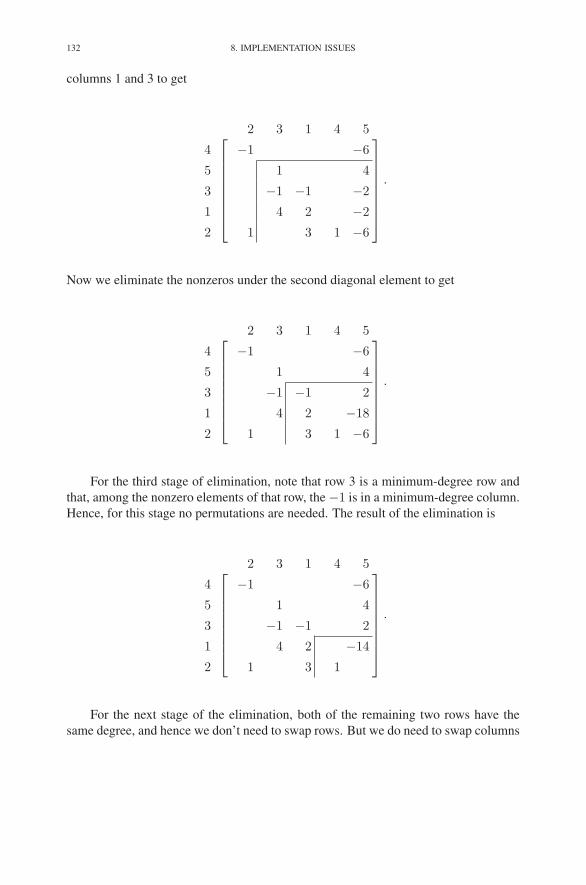
132 8. IMPLEMENTATION ISSUES
columns 1 and 3 to get
2 3 1 4 5
4
5
3
1
2
⎡
⎢
⎢
⎢
⎢
⎢
⎢
⎢
⎣
−1 −6
1 4
−1 −1 −2
4 2 −2
1 3 1 −6
⎤
⎥
⎥
⎥
⎥
⎥
⎥
⎥
⎦
.
Now we eliminate the nonzeros under the second diagonal element to get
2 3 1 4 5
4
5
3
1
2
⎡
⎢
⎢
⎢
⎢
⎢
⎢
⎢
⎣
−1 −6
1 4
−1 −1 2
4 2 −18
1 3 1 −6
⎤
⎥
⎥
⎥
⎥
⎥
⎥
⎥
⎦
.
For the third stage of elimination, note that row 3 is a minimum-degree row and
that, among the nonzero elements of that row, the −1 is in a minimum-degree column.
Hence, for this stage no permutations are needed. The result of the elimination is
2 3 1 4 5
4
5
3
1
2
⎡
⎢
⎢
⎢
⎢
⎢
⎢
⎢
⎣
−1 −6
1 4
−1 −1 2
4 2 −14
1 3 1
⎤
⎥
⎥
⎥
⎥
⎥
⎥
⎥
⎦
.
For the next stage of the elimination, both of the remaining two rows have the
same degree, and hence we don’t need to swap rows. But we do need to swap columns
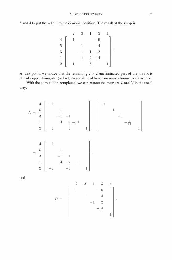
2. EXPLOITING SPARSITY 133
5 and 4 to put the −14 into the diagonal position. The result of the swap is
2 3 1 5 4
4
5
3
1
2
⎡
⎢
⎢
⎢
⎢
⎢
⎢
⎢
⎣
−1 −6
1 4
−1 −1 2
4 2 −14
1 3 1
⎤
⎥
⎥
⎥
⎥
⎥
⎥
⎥
⎦
.
At this point, we notice that the remaining 2 × 2 uneliminated part of the matrix is
already upper triangular (in fact, diagonal), and hence no more elimination is needed.
With the elimination completed, we can extract the matrices L and U in the usual
way:
L =
4
5
3
1
2
⎡
⎢
⎢
⎢
⎢
⎢
⎢
⎢
⎣
−1
1
−1 −1
4 2 −14
1 3 1
⎤
⎥
⎥
⎥
⎥
⎥
⎥
⎥
⎦
⎡
⎢
⎢
⎢
⎢
⎢
⎢
⎢
⎣
−1
1
−1
− 114
1
⎤
⎥
⎥
⎥
⎥
⎥
⎥
⎥
⎦
=
4
5
3
1
2
⎡
⎢
⎢
⎢
⎢
⎢
⎢
⎢
⎣
1
1
−1 1
4 −2 1
−1 −3 1
⎤
⎥
⎥
⎥
⎥
⎥
⎥
⎥
⎦
,
and
U =
2 3 1 5 4⎡
⎢
⎢
⎢
⎢
⎢
⎢
⎢
⎣
−1 −6
1 4
−1 2
−14
1
⎤
⎥
⎥
⎥
⎥
⎥
⎥
⎥
⎦
.

134 8. IMPLEMENTATION ISSUES
(Note that the columns of L and the rows of U do not have any “original” indices
associated with them, and so no permutation is indicated across the top of L or down
the left side of U .)
This LU -factorization has five off-diagonal nonzeros in L and three off-diagonal
nonzeros in U for a total of eight off-diagonal nonzeros. In contrast, the LU factor-
ization from the previous section had a total of 12 off-diagonal nonzeros. Hence, the
minimum-degree ordering heuristic paid off for this example by reducing the number
of nonzeros by 33%. While such a reduction may not seem like a big deal for small
matrices such as our 5× 5 example, for large matrices the difference can be dramatic.
The fact that we have permuted the rows and columns to get this factorization has
only a small impact on how one uses the factorization to solve systems of equations.
To illustrate, let us solve the same system that we considered before: B∆xB = aj ,
where aj is given by (8.3). The first step in solving this system is to permute the rows
of aj so that they agree with the rows of L and then to use forward substitution to
solve the system Ly = aj . Writing it out, the system looks like this:
4
5
3
1
2
⎡
⎢
⎢
⎢
⎢
⎢
⎢
⎢
⎣
1
1
−1 1
4 −2 1
−1 −3 1
⎤
⎥
⎥
⎥
⎥
⎥
⎥
⎥
⎦
⎡
⎢
⎢
⎢
⎢
⎢
⎢
⎢
⎣
y1
y2
y3
y4
y5
⎤
⎥
⎥
⎥
⎥
⎥
⎥
⎥
⎦
=
4
5
3
1
2
⎡
⎢
⎢
⎢
⎢
⎢
⎢
⎢
⎣
3
0
0
7
−2
⎤
⎥
⎥
⎥
⎥
⎥
⎥
⎥
⎦
The result of the forward substitution is that
(8.4)
⎡
⎢
⎢
⎢
⎢
⎢
⎢
⎢
⎣
y1
y2
y3
y4
y5
⎤
⎥
⎥
⎥
⎥
⎥
⎥
⎥
⎦
=
⎡
⎢
⎢
⎢
⎢
⎢
⎢
⎢
⎣
3
0
0
7
1
⎤
⎥
⎥
⎥
⎥
⎥
⎥
⎥
⎦
.
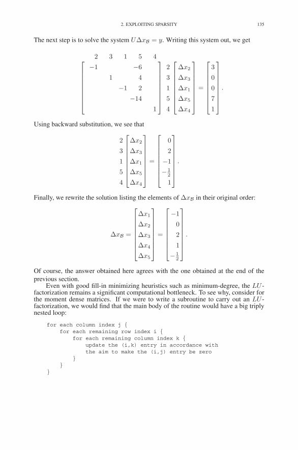
2. EXPLOITING SPARSITY 135
The next step is to solve the system U∆xB = y. Writing this system out, we get
2 3 1 5 4⎡
⎢
⎢
⎢
⎢
⎢
⎢
⎢
⎣
−1 −6
1 4
−1 2
−14
1
⎤
⎥
⎥
⎥
⎥
⎥
⎥
⎥
⎦
2
3
1
5
4
⎡
⎢
⎢
⎢
⎢
⎢
⎢
⎢
⎣
∆x2
∆x3
∆x1
∆x5
∆x4
⎤
⎥
⎥
⎥
⎥
⎥
⎥
⎥
⎦
=
⎡
⎢
⎢
⎢
⎢
⎢
⎢
⎢
⎣
3
0
0
7
1
⎤
⎥
⎥
⎥
⎥
⎥
⎥
⎥
⎦
.
Using backward substitution, we see that
2
3
1
5
4
⎡
⎢
⎢
⎢
⎢
⎢
⎢
⎢
⎣
∆x2
∆x3
∆x1
∆x5
∆x4
⎤
⎥
⎥
⎥
⎥
⎥
⎥
⎥
⎦
=
⎡
⎢
⎢
⎢
⎢
⎢
⎢
⎢
⎣
0
2
−1
− 12
1
⎤
⎥
⎥
⎥
⎥
⎥
⎥
⎥
⎦
.
Finally, we rewrite the solution listing the elements of ∆xB in their original order:
∆xB =
⎡
⎢
⎢
⎢
⎢
⎢
⎢
⎢
⎣
∆x1
∆x2
∆x3
∆x4
∆x5
⎤
⎥
⎥
⎥
⎥
⎥
⎥
⎥
⎦
=
⎡
⎢
⎢
⎢
⎢
⎢
⎢
⎢
⎣
−1
0
2
1
− 12
⎤
⎥
⎥
⎥
⎥
⎥
⎥
⎥
⎦
.
Of course, the answer obtained here agrees with the one obtained at the end of the
previous section.Even with good fill-in minimizing heuristics such as minimum-degree, the LU -
factorization remains a significant computational bottleneck. To see why, consider forthe moment dense matrices. If we were to write a subroutine to carry out an LU -factorization, we would find that the main body of the routine would have a big triplynested loop:
for each column index j {for each remaining row index i {
for each remaining column index k {update the (i,k) entry in accordance withthe aim to make the (i,j) entry be zero
}}
}
136 8. IMPLEMENTATION ISSUES
Since each of these loops involves approximately m steps, the LU -factorization rou-
tine requires about m3 operations and hence is called an order m3 algorithm. Similar
considerations tell us that the forward and backward substitutions are both order m2
algorithms. This means that forward and backward substitution can be done much
faster than LU -factorization. Indeed, if m = 5000, then factorization takes a couple
of thousand times longer than a forward or backward substitution. Of course, this ar-
gument is for dense matrices. But for sparse matrices a similar, if less dramatic, effect
is seen. Typically, for sparse matrices, one expects that factorization will take from
10 to 100 times longer than substitution. Therefore, it is important to perform as few
LU -factorizations as possible. This is the subject of the next section.
3. Reusing a Factorization
In the previous two sections, we showed how to use an LU -factorization of B to
solve the system of equations
B∆xB = aj
for the primal step direction ∆xB. Since the basis matrix doesn’t change much from
one iteration of the simplex method to the next (columns get replaced by new ones
one at a time), we ask whether the LU -factorization of B from the current iteration
might somehow be used again to solve the systems of equations that arise in the next
iteration (or even the next several iterations).
Let B denote the current basis (for which a factorization has already been com-
puted) and let B denote the basis of the next iteration. Then B is simply B with
the column that holds the column vector ai associated with the leaving variable xi
replaced by a new column vector aj associated with the entering variable xj . This
verbal description can be converted into a formula:
(8.5) B = B + (aj − ai)eTi .
Here, as before, ei denotes the vector that is all zeros except for a one in the position
associated with index i—to be definite, let us say that this position is the pth position
in the vector. To see why this formula is correct, it is helpful to realize that a column
vector, say a, times eTi produces a matrix that is all zero except for the pth column,
which contains the column vector a.
Since the basis B is invertible, (8.5) can be rewritten as
B = B(
I + B−1(aj − ai)eTi
)
.
Denote the matrix in parentheses by E. Recall that aj = Nej , since it is the column
vector from A associated with the entering variable xj . Hence,
B−1aj = B−1Nej = ∆xB,

3. REUSING A FACTORIZATION 137
which is a vector we need to compute in the current iteration anyway. Also,
B−1ai = ei,
since ai is the column of B associated with the leaving variable xi. Therefore, we can
write E more simply as
E = I + (∆xB − ei)eTi .
Now, if E has a simple inverse, then we can use it together with the LU -factorization
of B to provide an efficient means of solving systems of equations involving B. The
following proposition shows that E does indeed have a simple inverse.
PROPOSITION 8.1. Given two column vectors u and v for which 1 + vT u �= 0,
(I + uvT )−1 = I − uvT
1 + vT u.
PROOF. The proof is trivial. We simply multiply the matrix by its supposed in-
verse and check that we get the identity:
(
I + uvT)
(
I − uvT
1 + vT u
)
= I + uvT − uvT
1 + vT u− uvT uvT
1 + vT u
= I + uvT
(
1 − 1
1 + vT u− vT u
1 + vT u
)
= I,
where the last equality follows from the observation that the parenthesized expression
vanishes. �
The identity in Proposition 8.1 may seem mysterious, but in fact it has a simple
derivation based on the explicit formula for the sum of a geometric series:
∞∑
j=0
ξj =1
1 − ξ, for |ξ| < 1.
This is an identity for real numbers, but it also holds for matrices:
∞∑
j=0
Xj = (I − X)−1
,
provided that the absolute value of each of the eigenvalues of X is less than one (we
don’t prove this here, since it’s just for motivation). Assuming, for the moment, that
the absolute values of the eigenvalues of uvT are less than one (actually, all but one of
them are zero), we can expand (I+uvT )−1 in a geometric series, reassociate products,
138 8. IMPLEMENTATION ISSUES
and collapse the resulting geometric series to get(
I + uvT)−1
= I − uvT + (uvT )(uvT ) − (uvT )(uvT )(uvT ) + · · ·= I − uvT + u(vT u)vT − u(vT u)(vT u)vT + · · ·= I − u
(
1 − vT u + (vT u)2 − · · ·)
vT
= I − u1
1 + vT uvT
= I − uvT
1 + vT u,
where the last equality follows from the fact that 1/(1+ vT u) is a scalar and therefore
can be pulled out of the vector/matrix calculation.
Applying Proposition 8.1 to matrix E, we see that
E−1 = I − (∆xB − ei)eTi
1 + eTi (∆xB − ei)
= I − (∆xB − ei)eTi
∆xi
=
⎡
⎢
⎢
⎢
⎢
⎢
⎢
⎢
⎢
⎢
⎢
⎢
⎢
⎢
⎢
⎣
1 −∆xj1
∆xi
. . .
1 −∆xjp−1
∆xi
1∆xi
−∆xjp+1
∆xi1
. . .
−∆xjm
∆xi1
⎤
⎥
⎥
⎥
⎥
⎥
⎥
⎥
⎥
⎥
⎥
⎥
⎥
⎥
⎥
⎦
.
Now, let’s look at the systems of equations that need to be solved in the next
iteration. Using tildes to denote items associated with the next iteration, we see that
we need to solve
B∆xB = aj and BT v = ei
(actually, we should probably put the tilde on the j instead of the aj and on the iinstead of the ei, but doing so seems less aesthetically appealing, even though it’s
more correct). Recalling that B = BE, we see that the first system is equivalent to
BE∆xB = aj ,
which can be solved in two stages:
Bu = aj ,
E∆xB = u.

3. REUSING A FACTORIZATION 139
Of course, the second system (involving E) is trivial, since we have an explicit formula
for the inverse of E:
∆xB = E−1u
= u − ui
∆xi(∆xB − ei)
(where, in keeping with our tradition, we have used ui to denote the element of uassociated with the basic variable xi—that is, ui is the pth entry of u).
The system involving BT is handled in the same manner. Indeed, first we rewrite
it as
ET BT v = ei
and then observe that it too can be solved in two steps:
ET u = ei,
BT v = u.
This time, the first step is the trivial one1:
u = E−T ei
= ei − ei(∆xB − ei)
T ei
∆xi.
Note that the fraction in the preceding equation is a scalar, and so this final expression
for u shows that it is a vector with at most two nonzeros—that is, the result is utterly
trivial even if the formula looks a little bit cumbersome.
We end this section by returning briefly to our example. Suppose that B is B with
column 3 replaced by the vector aj given in (8.3). Suppose that
aj =[
5 0 0 0−1]T
.
To solve B∆xB = aj , we first solve Bu = aj using our LU -factorization of B. The
result of the forward and backward substitutions is
u =[
0 3 1−3− 12
]T
.
1Occasionally we use the superscript −T for the transpose of the inverse of a matrix. Hence, E−T =(E−1)T .

140 8. IMPLEMENTATION ISSUES
Next, we solve for ∆xB = E−1u:
∆xB = u − u3
∆x3(∆xB − e3) =
⎡
⎢
⎢
⎢
⎢
⎢
⎢
⎢
⎣
0
3
1
−3
− 12
⎤
⎥
⎥
⎥
⎥
⎥
⎥
⎥
⎦
− 1
2
⎛
⎜
⎜
⎜
⎜
⎜
⎜
⎜
⎝
⎡
⎢
⎢
⎢
⎢
⎢
⎢
⎢
⎣
−1
0
2
1
− 12
⎤
⎥
⎥
⎥
⎥
⎥
⎥
⎥
⎦
−
⎡
⎢
⎢
⎢
⎢
⎢
⎢
⎢
⎣
0
0
1
0
0
⎤
⎥
⎥
⎥
⎥
⎥
⎥
⎥
⎦
⎞
⎟
⎟
⎟
⎟
⎟
⎟
⎟
⎠
=
⎡
⎢
⎢
⎢
⎢
⎢
⎢
⎢
⎣
12
312
− 72
− 14
⎤
⎥
⎥
⎥
⎥
⎥
⎥
⎥
⎦
.
Of course, it is easy to check that we have gotten the correct answer: simply multiply
B times ∆xB and check that it equals aj . It does.
4. Performance Tradeoffs
The idea of writing the next basis as a product of the current basis times an easily
invertible matrix can be extended over several iterations. For example, if we look kiterations out, we can write
Bk = B0E0E1 · · ·Ek−1.
If we have an LU -factorization of B0 and we have saved enough information to re-
construct each Ej , then we can use this product to solve systems of equations involv-
ing Bk.
Note that in order to reconstruct Ej , all we need to save is the primal step direction
vector ∆xjB (and an integer telling which column it goes in). In actual implementa-
tions, these vectors are stored in lists. For historical reasons, this list is called an
eta-file (and the matrices Ej are called eta matrices). Given the LU -factorization of
B0 and the eta-file, it is an easy matter to solve systems of equations involving either
B or BT . However, as k gets large, the amount of work required to go through the
entire eta-file begins to dominate the amount of work that would be required to simply
form a new LU -factorization of the current basis. Hence, the best strategy is to use an
eta-file but with periodic refactorization of the basis (and accompanied purging of the
eta-file).
The question then becomes: how often should one recompute a factorization of
the current basis? To answer this question, suppose that we know that it takes Farithmetic operations to form an LU -factorization (of a typical basis for the problem
at hand), S operations to do one forward/backward substitution, and E operations to
multiply by the inverse of one eta-matrix. Then the number of operations for the initial
iteration of the simplex method is F + 2S (since we need to do an LU -factorization
and two forward/backward substitutions—one for the system involving the basis and
the other for the system involving its transpose). Then, in the next iteration, we need
to do two forward/backward substitutions and two eta-inverse calculations. Each sub-
sequent iteration is the same as the previous, except that there are two extra eta-inverse

5. UPDATING A FACTORIZATION 141
calculations. Hence, the average number of arithmetic operations per iteration if we
refactorize after every K iterations is
T (K) =1
K((F + 2S) + 2(S + E) + 2(S + 2E)
+ · · · + 2(S + (K − 1)E))
=1
KF + 2S + (K − 1)E.
Treating K as a real variable for the moment, we can differentiate this expression with
respect to K, set the derivative equal to zero, and solve for K to get an estimate for
the optimal choice of K:
K =
√
F
E.
As should be clear from our earlier discussions, E is of order m and, if the basis
matrix is dense, F is of order m3. Hence, for dense matrices, our estimates would
indicate that refactorizations should take place every m iterations or so. However,
for sparse matrices, F will be substantially less that m3—more like a constant times
m2—which would indicate that refactorizations should occur on the order of every√m iterations. In practice, one typically allows the value of K to be a user-settable
parameter whose default value is set to something like 100.
5. Updating a Factorization
There is an important alternative to the eta-matrix method for reusing an LU -
factorization, which we shall describe in this section and the next. As always, it is
easiest to work with an example, so let’s continue with the same example we’ve been
using throughout this chapter.
Recall that the matrix B is simply B with its third column replaced by the vector
aj given in (8.3):
B =
1 2 3 4 5
1
2
3
4
5
⎡
⎢
⎢
⎢
⎢
⎢
⎢
⎢
⎣
2 7 −2
3 1 −2 1
−1 −2
−1 3 −6
4
⎤
⎥
⎥
⎥
⎥
⎥
⎥
⎥
⎦
=
2 3 1 5 4
4
5
3
1
2
⎡
⎢
⎢
⎢
⎢
⎢
⎢
⎢
⎣
−1 3 −6
4
−1 −2
7 2 −2
1 −2 3 1
⎤
⎥
⎥
⎥
⎥
⎥
⎥
⎥
⎦
.
(Note that we’ve highlighted the new column by putting a box around it.)
Since L−1B = U and B differs from B in only one column, it follows that L−1Bcoincides with U except for the column that got changed. And, since this column got

142 8. IMPLEMENTATION ISSUES
replaced by aj , it follows that this column of L−1B contains L−1aj , which we’ve
already computed and found to be given by (8.4). Hence,
(8.6) L−1B =
2 3 1 5 4
1
2
3
4
5
⎡
⎢
⎢
⎢
⎢
⎢
⎢
⎢
⎣
−1 3 −6
4
−1 2
7 −14
1 1
⎤
⎥
⎥
⎥
⎥
⎥
⎥
⎥
⎦
.
As we saw before, the columns of L have no “original” indices to relate back to, and
so one can simply take them to be numbered in natural order. The same is then true
for the rows of L−1 and hence for the rows of L−1B. That is why the rows shown
above are numbered as they are. We’ve shown these numbers explicitly, since they are
about to get permuted.
The boxed column in (8.6) is called a spike, since it has nonzeros below the diag-
onal. The 4×4 submatrix constructed from rows 2 through 5 and columns 3, 1, 5, and
4 is called the bump. To get this matrix back into upper-triangular form, one could do
row operations to eliminate the nonzeros in the spike that lie below the diagonal. But
such row operations could create fill-in anywhere in the bump. Such fill-in would be
more than one would like to encounter. However, consider what happens if the spike
column is moved to the rightmost column of the bump, shifting the other columns left
one position in the process, and if the top row of the bump (i.e., row 2) is moved to
the bottom of the bump, shifting the other bump rows up by one. The result of these
permutations is
L−1B =
2 1 5 4 3
1
3
4
5
2
⎡
⎢
⎢
⎢
⎢
⎢
⎢
⎢
⎣
−1 −6 3
−1 2
−14 7
1 1
4
⎤
⎥
⎥
⎥
⎥
⎥
⎥
⎥
⎦
.
(For future reference, we’ve boxed the bump.) In general, the effect of this permutation
is that the column spike gets replaced by a row spike along the bottom row of the bump:

5. UPDATING A FACTORIZATION 143
⎡
⎢
⎢
⎢
⎢
⎢
⎢
⎢
⎢
⎢
⎢
⎢
⎢
⎢
⎢
⎢
⎢
⎢
⎢
⎢
⎢
⎢
⎣
∗ ∗ ∗ ∗ ∗ ∗ ∗ ∗ ∗ ∗ ∗∗ ∗ ∗ ∗ ∗ ∗ ∗ ∗ ∗ ∗
∗ ∗ ∗ ∗ ∗ ∗ ∗ ∗ ∗∗ ∗ ∗ ∗ ∗ ∗ ∗ ∗ ∗∗ ∗ ∗ ∗ ∗ ∗ ∗ ∗∗ ∗ ∗ ∗ ∗ ∗ ∗∗ ∗ ∗ ∗ ∗ ∗∗ ∗ ∗ ∗ ∗∗ ∗ ∗ ∗
∗ ∗∗
⎤
⎥
⎥
⎥
⎥
⎥
⎥
⎥
⎥
⎥
⎥
⎥
⎥
⎥
⎥
⎥
⎥
⎥
⎥
⎥
⎥
⎥
⎦
−→
⎡
⎢
⎢
⎢
⎢
⎢
⎢
⎢
⎢
⎢
⎢
⎢
⎢
⎢
⎢
⎢
⎢
⎢
⎢
⎢
⎢
⎢
⎣
∗ ∗ ∗ ∗ ∗ ∗ ∗ ∗ ∗ ∗ ∗∗ ∗ ∗ ∗ ∗ ∗ ∗ ∗ ∗ ∗
∗ ∗ ∗ ∗ ∗ ∗ ∗ ∗ ∗∗ ∗ ∗ ∗ ∗ ∗ ∗ ∗
∗ ∗ ∗ ∗ ∗ ∗ ∗∗ ∗ ∗ ∗ ∗ ∗
∗ ∗ ∗ ∗ ∗∗ ∗ ∗ ∗
∗ ∗ ∗ ∗ ∗ ∗ ∗ ∗ ∗∗ ∗
∗
⎤
⎥
⎥
⎥
⎥
⎥
⎥
⎥
⎥
⎥
⎥
⎥
⎥
⎥
⎥
⎥
⎥
⎥
⎥
⎥
⎥
⎥
⎦
.
Now any fill-in produced by row operations is confined to the spike row. In our exam-
ple, there is only one nonzero in the spike row, and to eliminate it we need to add 2/7times row 4 to it. This row operation can be represented algebraically as multiplication
on the left by the matrix
E =
⎡
⎢
⎢
⎢
⎢
⎢
⎢
⎢
⎣
1
1
1
127 1
⎤
⎥
⎥
⎥
⎥
⎥
⎥
⎥
⎦
.
That is,
EL−1B =
2 1 5 4 3
1
3
4
5
2
⎡
⎢
⎢
⎢
⎢
⎢
⎢
⎢
⎣
−1 −6 3
−1 2
−14 7
1 1
2
⎤
⎥
⎥
⎥
⎥
⎥
⎥
⎥
⎦
.
If we denote the new upper triangular matrix by U , then, solving for B, we get the
following factorization of B:
B = LE−1U .
We can use this new factorization to solve systems of equations. For example, to
solve
B∆xB = aj ,
we first solve
(8.7) Ly = aj
for y. Then, given y, we compute
z = Ey,

144 8. IMPLEMENTATION ISSUES
and finally we solve
U∆xB = z
for ∆xB. It is clear from the following chain of equalities that these three steps com-
pute ∆xB:
∆xB = U−1z = U−1Ey = U−1EL−1aj = B−1aj .
For our example, we use forward substitution to solve (8.7) for y. The result is
y =
1
2
3
4
5
⎡
⎢
⎢
⎢
⎢
⎢
⎢
⎢
⎣
0
−1
−1
7
−3
⎤
⎥
⎥
⎥
⎥
⎥
⎥
⎥
⎦
=
1
3
4
5
2
⎡
⎢
⎢
⎢
⎢
⎢
⎢
⎢
⎣
0
−1
7
−3
−1
⎤
⎥
⎥
⎥
⎥
⎥
⎥
⎥
⎦
.
Next, we apply the row operations (in our case, there is only one) to get z:
z = Ey =
1
3
4
5
2
⎡
⎢
⎢
⎢
⎢
⎢
⎢
⎢
⎣
0
−1
7
−3
1
⎤
⎥
⎥
⎥
⎥
⎥
⎥
⎥
⎦
.
Finally, backward substitution using U is performed to compute ∆xB:
2 1 5 4 3
1
3
4
5
2
⎡
⎢
⎢
⎢
⎢
⎢
⎢
⎢
⎣
−1 −6 3
−1 2
−14 7
1 1
2
⎤
⎥
⎥
⎥
⎥
⎥
⎥
⎥
⎦
2
1
5
4
3
⎡
⎢
⎢
⎢
⎢
⎢
⎢
⎢
⎣
?
⎤
⎥
⎥
⎥
⎥
⎥
⎥
⎥
⎦
=
1
3
4
5
2
⎡
⎢
⎢
⎢
⎢
⎢
⎢
⎢
⎣
0
−1
7
−3
1
⎤
⎥
⎥
⎥
⎥
⎥
⎥
⎥
⎦
.
The result of the backward substitution is
∆xB =
2
1
5
4
3
⎡
⎢
⎢
⎢
⎢
⎢
⎢
⎢
⎣
312
− 14
− 7212
⎤
⎥
⎥
⎥
⎥
⎥
⎥
⎥
⎦
=
1
2
3
4
5
⎡
⎢
⎢
⎢
⎢
⎢
⎢
⎢
⎣
12
312
− 72
− 14
⎤
⎥
⎥
⎥
⎥
⎥
⎥
⎥
⎦
,
which agrees with the solution we got before using eta-matrices.

6. SHRINKING THE BUMP 145
6. Shrinking the Bump
There is an important enhancement to the factorization updating technique de-
scribed in the previous section. After permuting rows and columns converting the
spike column into a spike row, we can exploit the fact that the spike row is often very
sparse (coming as it does from what was originally the top row of the bump) and do
further row and column permutations to reduce the size of the bump. To see what
we mean, let’s look at our example. First, we note that the leftmost element of the
spike row is zero (and hence that the left column of the bump is a singleton column).
Therefore, we can simply declare that this column and the corresponding top row do
not belong to the bump. That is, we can immediately reduce the size of the bump by
one:
2 1 5 4 3
1
3
4
5
2
⎡
⎢
⎢
⎢
⎢
⎢
⎢
⎢
⎣
−1 −6 3
−1 2
−14 7
1 1
4
⎤
⎥
⎥
⎥
⎥
⎥
⎥
⎥
⎦
.
This idea can be extended to any column that has a single nonzero in the bump. For
example, column 4 is a singleton column too. The trick now is to move this column to
the leftmost column of the bump, pushing the intermediate columns to the right, and
to apply the same permutation to the rows. After permuting the rows and columns like
this, the bump can be reduced in size again:
2 1 4 5 3
1
3
5
4
2
⎡
⎢
⎢
⎢
⎢
⎢
⎢
⎢
⎣
−1 −6 3
−1 2
1 1
−14 7
4
⎤
⎥
⎥
⎥
⎥
⎥
⎥
⎥
⎦
.
Furthermore, this reduction in the bump causes a new singleton column to appear
(since a singleton need only be a singleton within the bump), namely, column 3.
Hence, we permute once again. This time just the column gets permuted, since the
singleton is already in the correct row. The bump gets reduced in size once again, now

146 8. IMPLEMENTATION ISSUES
to a 1 × 1 bump, which is not really a bump at all:
2 1 4 3 5
1
3
5
4
2
⎡
⎢
⎢
⎢
⎢
⎢
⎢
⎢
⎣
−1 3 −6
−1 2
1 1
7 −14
4
⎤
⎥
⎥
⎥
⎥
⎥
⎥
⎥
⎦
.
Note that we have restored upper triangularity using only permutations; no row oper-
ations were needed. While this doesn’t always happen, it is a common and certainly
welcome event.
Our example, being fairly small, doesn’t exhibit all the possible bump-reducing
permutations. In addition to looking for singleton columns, one can also look for
singleton rows. Each singleton row can be moved to the bottom of the bump. At the
same time, the associated column is moved to the right-hand column of the bump.
After this permutation, the right-hand column and the bottom row can be removed
from the bump.
Before closing this section, we reiterate a few important points. First, as the
bump gets smaller, the chances of finding further singletons increases. Also, with the
exception of the lower-right diagonal element of the bump, all other diagonal elements
are guaranteed to be nonzero, since the matrix U from which U is derived has this
property. Therefore, most bump reductions apply the same permutation to the rows
as to the columns. Finally, we have illustrated how to update the factorization once,
but this technique can, of course, be applied over and over. Eventually, however, it
becomes more efficient to refactorize the basis from scratch.
7. Partial Pricing
In many real-world problems, the number of constraints m is small compared
with the number of variables n. Looking over the steps of the primal simplex method,
we see that the only steps involving n-vectors are Step 2, in which we pick a nonbasic
variable to be the entering variable,
pick j ∈ {j ∈ N : z∗j < 0};Step 6, in which we compute the step direction for the dual variables,
∆zN = −(B−1N)T ei;
and Step 8, in which we update the dual variables,
z∗N ← z∗N − s∆zN .
Scanning all the nonbasic indices in Step 2 requires looking at n candidates. When nis huge, this step is likely to be a bottleneck step for the algorithm. However, there is
8. STEEPEST EDGE 147
no requirement that all indices be scanned. We could simply scan from the beginning
and stop at the first index j for which z∗j is negative (as in Bland’s rule). However, in
practice, it is felt that picking an index j corresponding to a very negative z∗j produces
an algorithm that is likely to reach optimality faster. Therefore, the following scheme,
referred to as partial pricing is often employed. Initially, scan only a fraction of the
indices (say n/3), and set aside a handful of good ones (say, the 40 or so having the
most negative z∗j ). Then use only these 40 in Steps 2, 6, and 8 for subsequent iterations
until less than a certain fraction (say, 1/2) of them remain eligible. At this point, use
(6.8) to compute the current values of a new batch of n/3 nonbasic dual variables, and
go back to the beginning of this partial pricing process by setting aside the best 40. In
this way, most of the iterations look like they only have 40 nonbasic variables. Only
occasionly does the grim reality of the full huge number of nonbasic variables surface.
Looking at the dual simplex method (Figure 6.1), we see that we aren’t so lucky.
In it, vectors of length n arise in the max-ratio test:
t =
(
maxj∈N
∆zj
z∗j
)−1
pick j ∈ argmaxj∈N∆zj
z∗j.
Here, the entire collection of nonbasic indices must be checked; otherwise, dual fea-
sibility will be lost and the algorithm will fail. Therefore, in cases where n is huge
relative to m and partial pricing is used, it is important not to use the dual simplex
method as a Phase I procedure. Instead, one should use the technique of adding artifi-
cial variables as we did in Chapter 2 to force an initial feasible solution.
8. Steepest Edge
In Chapter 4, we saw that one of the drawbacks of the largest-coefficient rule is
its sensitivity to the scale in which variables are quantified. In this section, we shall
discuss a pivot rule that partially remedies this problem. Recall that each step of the
simplex method is a step along an edge of the feasible region from one vertex to an
adjacent vertex. The largest coefficient rule picks the variable that gives the largest
rate of increase of the objective function. However, this rate of increase is measured
in the “space of nonbasic variables” (we view the basic variables simply as dependent
variables). Also, this space changes from one iteration to the next. Hence, in a certain
respect, it would seem wiser to measure the rate of increase in the larger space consist-
ing of all the variables, both basic and nonbasic. When the rate of increase is gauged
in this larger space, the pivot rule is called the steepest-edge rule. It is the subject of
this section.
148 8. IMPLEMENTATION ISSUES
Fix a nonbasic index j ∈ N . We wish to consider whether xj should be the
entering variable. If it were, the step direction vector would be
∆x =
[
∆xB
∆xN
]
=
[
−B−1Nej
ej
]
.
This vector points out along the edge corresponding to the pivot that would result by
letting xj enter the basis. As we know, the objective function is
f(x) = cT x = cTBxB + cT
NxN .
The derivative of f(x) in the direction of ∆x is given by
∂f
∂∆x= cT ∆x
‖∆x‖ =cTB∆xB + cT
N∆xN‖∆x‖ .
The numerator is easy (and familiar):
cTB∆xB + cT
N∆xN = cj − cTBB−1Nej
=(
cN − (B−1N)T cB)
j
=−z∗j .
The denominator is more troublesome:
‖∆x‖2 = ‖∆xB‖2 + 1 = ‖B−1Nej‖2 + 1.
To calculate B−1Nej for every j ∈ N is exactly the same as computing the matrix
B−1N , which (as we’ve discussed before) is time consuming and therefore a com-
putation we wish to avoid. But it turns out that we can compute B−1Nej for every
j ∈ N once at the start (when B is essentially, if not identically, an identity matrix)
and then update the norms of these vectors using a simple formula, which we shall
now derive.
Let
νk = ‖B−1Nek‖2, k ∈ N .
Suppose that we know these numbers, we use them to perform one step of the simplex
method, and we are now at the beginning of the next iteration. As usual, let us denote
quantities in this next iteration by putting tildes on them. For example, B denotes the
new basis matrix. As we’ve seen before, B is related to B by the equation B = BE,
where
E−1 = I − (∆xB − ei)eTi
∆xi.
Now, let’s compute the new ν values:
νk = aTk B−T B−1ak
= aTk B−T E−T E−1B−1ak
= aTk B−T
(
I − ei(∆xB − ei)T
∆xi
)(
I − (∆xB − ei)eTi
∆xi
)
B−1ak.(8.8)
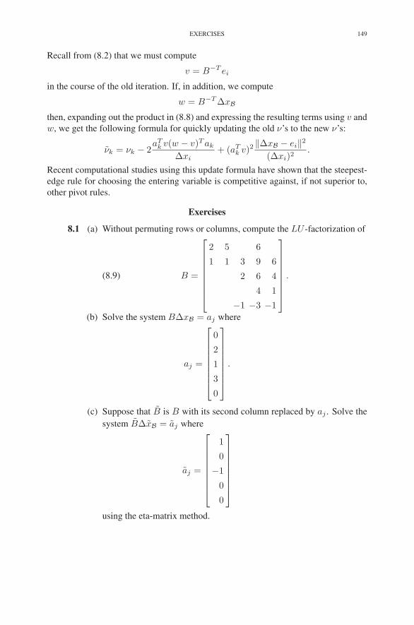
EXERCISES 149
Recall from (8.2) that we must compute
v = B−T ei
in the course of the old iteration. If, in addition, we compute
w = B−T ∆xB
then, expanding out the product in (8.8) and expressing the resulting terms using v and
w, we get the following formula for quickly updating the old ν’s to the new ν’s:
νk = νk − 2aT
k v(w − v)T ak
∆xi+ (aT
k v)2‖∆xB − ei‖2
(∆xi)2.
Recent computational studies using this update formula have shown that the steepest-
edge rule for choosing the entering variable is competitive against, if not superior to,
other pivot rules.
Exercises
8.1 (a) Without permuting rows or columns, compute the LU -factorization of
(8.9) B =
⎡
⎢
⎢
⎢
⎢
⎢
⎢
⎢
⎣
2 5 6
1 1 3 9 6
2 6 4
4 1
−1 −3 −1
⎤
⎥
⎥
⎥
⎥
⎥
⎥
⎥
⎦
.
(b) Solve the system B∆xB = aj where
aj =
⎡
⎢
⎢
⎢
⎢
⎢
⎢
⎢
⎣
0
2
1
3
0
⎤
⎥
⎥
⎥
⎥
⎥
⎥
⎥
⎦
.
(c) Suppose that B is B with its second column replaced by aj . Solve the
system B∆xB = aj where
aj =
⎡
⎢
⎢
⎢
⎢
⎢
⎢
⎢
⎣
1
0
−1
0
0
⎤
⎥
⎥
⎥
⎥
⎥
⎥
⎥
⎦
using the eta-matrix method.
150 8. IMPLEMENTATION ISSUES
(d) Solve the system B∆xB = aj again, this time using the factorization
updating method.
8.2 Use the minimum-degree ordering heuristic to find an LU -factorization of
the matrix B given by (8.9).
8.3 A permutation matrix is a matrix of zeros and ones for which each row has
one 1 and each column has one 1.
(a) Let B be an m × m matrix, and let P be a permutation matrix. Show
that PB is a matrix obtained by permuting the rows of B and that
BP is a matrix obtained by permuting the columns of B. Are the two
permutations the same?
(b) Show that every permutation of the rows of a matrix B corresponds to
multiplying B on the left by a permutation matrix.
(c) Show that for any permutation matrix P ,
P−1 = PT .
8.4 Explain how to use the factorization B = LU to solve
BT x = b.
Notes
Techniques for exploiting sparsity in matrix factorization have their roots in the
paper by Markowitz (1957). A few standard references on matrix factorization are the
books of Duff et al. (1986), Golub & VanLoan (1989), and Gill et al. (1991). The
eta-matrix technique given in Section 8.3 for using an old basis to solve systems of
equations involving the current basis was first described by Dantzig & Orchard-Hayes
(1954). The factorization updating technique described in Section 8.5 is the method
given by Forrest & Tomlin (1972). The bump reduction techniques of Section 8.6
were first introduced by Saunders (1973) and Reid (1982). The steepest-edge pivoting
rule is due to Goldfarb & Reid (1977). A similar rule, known as Devex, was given by
Harris (1973).
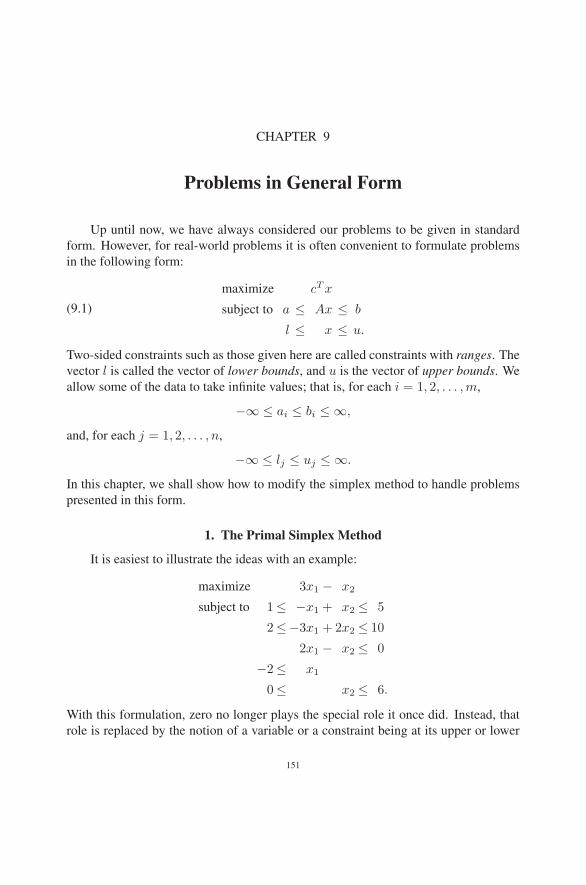
CHAPTER 9
Problems in General Form
Up until now, we have always considered our problems to be given in standard
form. However, for real-world problems it is often convenient to formulate problems
in the following form:
(9.1)
maximize cT x
subject to a ≤ Ax ≤ b
l ≤ x ≤ u.
Two-sided constraints such as those given here are called constraints with ranges. The
vector l is called the vector of lower bounds, and u is the vector of upper bounds. We
allow some of the data to take infinite values; that is, for each i = 1, 2, . . . ,m,
−∞ ≤ ai ≤ bi ≤ ∞,
and, for each j = 1, 2, . . . , n,
−∞ ≤ lj ≤ uj ≤ ∞.
In this chapter, we shall show how to modify the simplex method to handle problems
presented in this form.
1. The Primal Simplex Method
It is easiest to illustrate the ideas with an example:
maximize 3x1 − x2
subject to 1≤ −x1 + x2 ≤ 5
2≤−3x1 + 2x2 ≤ 10
2x1 − x2 ≤ 0
−2≤ x1
0≤ x2 ≤ 6.
With this formulation, zero no longer plays the special role it once did. Instead, that
role is replaced by the notion of a variable or a constraint being at its upper or lower
151

152 9. PROBLEMS IN GENERAL FORM
bound. Therefore, instead of defining slack variables for each constraint, we use wi
simply to denote the value of the ith constraint:
w1 = −x1 + x2
w2 =−3x1 + 2x2
w3 = 2x1 − x2.
The constraints can then be interpreted as upper and lower bounds on these variables.
Now when we record our problem in a dictionary, we will have to keep explicit track
of the upper and lower bound on the original xj variables and the new wi variables.
Also, the value of a nonbasic variable is no longer implicit; it could be at either its
upper or its lower bound. Hence, we shall indicate which is the case by putting a box
around the relevant bound. Finally, we need to keep track of the values of the basic
variables. Hence, we shall write our dictionary as follows:
l −2 0
u ∞ 6
ζ = 3x1 − x2 =−6
1 5 w1 = −x1 + x2 = 2
2 10 w2 =−3x1 + 2x2 = 6
−∞ 0 w3 = 2x1 − x2 =−4 .
Since all the wi’s are between their upper and lower bounds, this dictionary is feasi-
ble. But it is not optimal, since x1 could be increased from its present value at the
lower bound, thereby increasing the objective function’s value. Hence, x1 shall be the
entering variable for the first iteration. Looking at w1, we see that x1 can be raised
only 1 unit before w1 hits its lower bound. Similarly, x1 can be raised by 4/3 units,
at which point w2 hits its lower bound. Finally, if x1 were raised 2 units, then w3
would hit its upper bound. The tightest of these constraints is the one on w1, and so
w1 becomes the leaving variable—which, in the next iteration, will then be at its lower
bound. Performing the usual row operations, we get
l 1 0
u 5 6
ζ =−3w1 + 2x2 =−3
−2∞ x1 = −w1 + x2 =−1
2 10 w2 = 3w1 − x2 = 3
−∞ 0 w3 =−2w1 + x2 =−2 .
Note, of course, that the objective function value has increased (from −6 to −3). For
the second iteration, raising x2 from its lower bound will produce an increase in ζ.
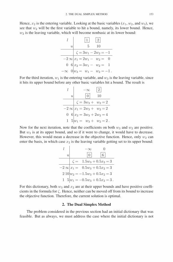
2. THE DUAL SIMPLEX METHOD 153
Hence, x2 is the entering variable. Looking at the basic variables (x1, w2, and w3), we
see that w2 will be the first variable to hit a bound, namely, its lower bound. Hence,
w2 is the leaving variable, which will become nonbasic at its lower bound:
l 1 2
u 5 10
ζ = 3w1 − 2w2 =−1
−2∞ x1 = 2w1 − w2 = 0
0 6 x2 = 3w1 − w2 = 1
−∞ 0 w3 = w1 − w2 =−1 .
For the third iteration, w1 is the entering variable, and w3 is the leaving variable, since
it hits its upper bound before any other basic variables hit a bound. The result is
l −∞ 2
u 0 10
ζ = 3w3 + w2 = 2
−2∞ x1 = 2w3 + w2 = 2
0 6 x2 = 3w3 + 2w2 = 4
1 5 w1 = w3 + w2 = 2 .
Now for the next iteration, note that the coefficients on both w3 and w2 are positive.
But w3 is at its upper bound, and so if it were to change, it would have to decrease.
However, this would mean a decrease in the objective function. Hence, only w2 can
enter the basis, in which case x2 is the leaving variable getting set to its upper bound:
l −∞ 0
u 0 6
ζ = 1.5w3 + 0.5x2 = 3
−2∞ x1 = 0.5w3 + 0.5x2 = 3
2 10 w2 =−1.5w3 + 0.5x2 = 3
1 5 w1 =−0.5w3 + 0.5x2 = 3 .
For this dictionary, both w3 and x2 are at their upper bounds and have positive coeffi-
cients in the formula for ζ. Hence, neither can be moved off from its bound to increase
the objective function. Therefore, the current solution is optimal.
2. The Dual Simplex Method
The problem considered in the previous section had an initial dictionary that was
feasible. But as always, we must address the case where the initial dictionary is not
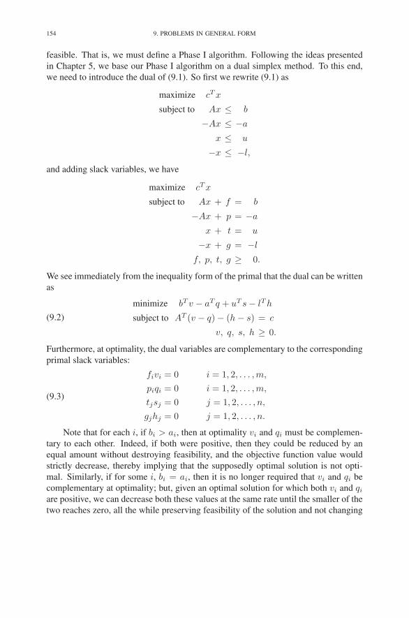
154 9. PROBLEMS IN GENERAL FORM
feasible. That is, we must define a Phase I algorithm. Following the ideas presented
in Chapter 5, we base our Phase I algorithm on a dual simplex method. To this end,
we need to introduce the dual of (9.1). So first we rewrite (9.1) as
maximize cT x
subject to Ax ≤ b
−Ax ≤ −a
x ≤ u
−x ≤ −l,
and adding slack variables, we have
maximize cT x
subject to Ax + f = b
−Ax + p = −a
x + t = u
−x + g = −l
f, p, t, g ≥ 0.
We see immediately from the inequality form of the primal that the dual can be written
as
(9.2)
minimize bT v − aT q + uT s − lT h
subject to AT (v − q) − (h − s) = c
v, q, s, h ≥ 0.
Furthermore, at optimality, the dual variables are complementary to the corresponding
primal slack variables:
(9.3)
fivi = 0 i = 1, 2, . . . ,m,
piqi = 0 i = 1, 2, . . . ,m,
tjsj = 0 j = 1, 2, . . . , n,
gjhj = 0 j = 1, 2, . . . , n.
Note that for each i, if bi > ai, then at optimality vi and qi must be complemen-
tary to each other. Indeed, if both were positive, then they could be reduced by an
equal amount without destroying feasibility, and the objective function value would
strictly decrease, thereby implying that the supposedly optimal solution is not opti-
mal. Similarly, if for some i, bi = ai, then it is no longer required that vi and qi be
complementary at optimality; but, given an optimal solution for which both vi and qi
are positive, we can decrease both these values at the same rate until the smaller of the
two reaches zero, all the while preserving feasibility of the solution and not changing

2. THE DUAL SIMPLEX METHOD 155
the objective function value. Hence, there always exists an optimal solution in which
every component of v is complementary to the corresponding component of q. The
same argument shows that if there exists an optimal solution, then there exists one in
which all the components of h and s are complementary to each other as well.
For a real variable ξ, its positive part ξ+ is defined as
ξ+ = max{ξ, 0}
and its negative part ξ− is defined similarly as
ξ− = max{−ξ, 0}.
Clearly, both ξ+ and ξ− are nonnegative. Furthermore, they are complementary,
ξ+ = 0 or ξ− = 0,
and their difference represents ξ:
ξ = ξ+ − ξ−.
From the complementarity of the components of v against the components of q,
we can think of them as the positive and negative parts of the components of just one
vector y. So let us write:
v = y+ and q = y−.
Similarly, let us write
h = z+ and s = z−.
If we impose these complementarity conditions not just at optimality but also from the
start, then we can eliminate v, q, s, and h from the dual and write it simply as
(9.4)minimize bT y+ − aT y− + uT z+ − lT z−
subject to AT y − z = c,
where the notation y+ denotes the componentwise positive part of y, etc. This problem
is an example from the class of problems called piecewise linear programs. Usually,
piecewise linear programs are solved by converting them into linear programs. Here,
however, we wish to go in the other direction. We shall present an algorithm for (9.4)
that will serve as an algorithm for (9.2). We will call this algorithm the dual simplex
method for problems in general form.
To economize on the presentation, we shall present the dual simplex method in
the context of a Phase I algorithm for linear programs in general form. Also, to avoid

156 9. PROBLEMS IN GENERAL FORM
cumbersome notations, we shall present the algorithm with the following example:
(9.5)
maximize 2x1 − x2
subject to 0≤ x1 + x2 ≤ 6
2≤−x1 + 2x2 ≤ 10
x1 − x2 ≤ 0
−2≤ x1
1≤ x2 ≤ 5.
The piecewise linear formulation of the dual is
minimize 6y+1 + 10y+
2 + 2z+1 − z+
2
− 2y−2 +∞y−
3 +∞z−1 + 5z−2subject to y1 − y2 + y3 − z1 = 2
y1 + 2y2 − y3 − − z2 =−1.
Note that the objective function has coefficients that are infinite. The correct
convention is that infinity times a variable is plus infinity if the variable is positive,
zero if the variable is zero, and minus infinity if the variable is negative.
Since the objective function is nonlinear (taking positive and negative parts of
variables is certainly a nonlinear operation), we will not be able to do the usual row
operations on the objective function. Therefore, in each iteration, we simply study it
as is. But as usual, we prefer to think in terms of maximization, and so we record the
negative of the objective function:
(9.6)−ξ =−6y+
1 − 10y+2 − 2z+
1 + z+2
+ 2y−2 −∞y−
3 −∞z−1 − 5z−2 .
We can of course perform row operations on the two constraints, so we set up the
usual sort of dictionary for them:
(9.7)z1 =−2 + y1 − y2 + y3
z2 = 1 + y1 + 2y2 − y3.
For the dual problem, all the action takes place at zero. That is, slopes in the objec-
tive function change when a variable goes from negative to positive. Since nonbasic
variable are supposed to be set where the action is, we associate a current solution
with each dictionary by setting the nonbasic variables to zero. Hence, the solution
associated with the initial dictionary is
(y1, y2, y3, z1, z2) = (0, 0, 0,−2, 1).
The fact that z1 is negative implies that z−1 is a positive number and hence that the
objective function value associated with this solution is minus infinity. Whenever the

2. THE DUAL SIMPLEX METHOD 157
objective function value is minus infinity, we say that the solution is infeasible. We
also refer to the associated dictionary as infeasible. Hence, the initial dictionary given
in (9.7) is infeasible.
The dual simplex method must start with a dual feasible solution. But since we
intend to use the dual simplex method simply to find a feasible solution for (9.5), we
are free to change the objective function in (9.5) any way we please. In particular, we
can change it from
ζ = 2x1 − x2
to
η = −2x1 − x2.
Making that change to the primal leaves the dual objective function unchanged, but
produces a feasible dual dictionary:
(9.8)z1 = 2 + y1 − y2 + y3
z2 = 1 + y1 + 2y2 − y3.
For comparison purposes, let us also record the corresponding primal dictionary.
It is easy to write down the equations defining the wi’s, but how do we know whether
the xj’s are supposed to be at their upper or their lower bounds? The answer comes
from the requirement that the primal and dual satisfy the complementarity conditions
given in (9.3). Indeed, from the dual dictionary we see that z1 = 1. Hence, z+1 = 1.
But since z+1 is just a surrogate for h1, we see that h1 is positive and hence that g1
must be zero. This means that x1 must be at its lower bound. Similarly, for the sake
of complementarity, x2 must also be at its lower bound. Hence, the primal dictionary
is
l −2 1
u ∞ 5
η = −x1 − x2 = 1
0 6 w1 = x1 + x2 =−1
2 10 w2 = −x1 + 2x2 = 4
−∞ 0 w3 = x1 − x2 =−3 .
Note that it is infeasible, since w1 is not between its upper and lower bounds.
We are now ready to describe the first iteration of the dual simplex method. To
this end, we ask whether we can improve the dual objective function value by moving
one of the nonbasic variables (y1, y2, or y3) away from zero. Of course, each of these
three variables can be moved either to the positive or the negative side of zero; we
must analyze these six cases individually. First of all, note that since z1 is positive at
the current solution, it follows that z+1 = z1 and z−1 = 0 in a neighborhood of the
current solution. A similar statement can be made for z2, and so we can rewrite (9.6)

158 9. PROBLEMS IN GENERAL FORM
locally around the current solution as
−ξ =−6y+1 − 10y+
2 − 2z1 + z2
+ 2y−2 −∞y−
3 .
Now, as y1 is increased from zero, the rate of increase of −ξ is simply the derivative of
the right-hand side with respect to y1, where we must keep in mind that z1 and z2 are
functions of y1 via the dictionary (9.8). Hence, the rate of increase is −6−2+1 = −7;
i.e., the objective function decreases at a rate of 7 units per unit increase of y1. If,
on the other hand, y2 is decreased from zero into negative territory, then the rate of
increase of −ξ is the negative of the derivative of the right-hand side. In this case
we get no contribution from y−1 but we do get something from z1 and z2 for a total
of 2 − 1 = 1. Hence, the rate of increase as we move in this direction is one unit
increase per unit move. We can analyze changes to y2 and y3. The entire situation can
be summarized as follows:
y1 ր −6− 2 + 1 = −7
y1 ց 0 + 2− 1 = 1
y2 ր−10 + 2 + 2 = −6
y2 ց 2− 2− 2 = −2
y3 ր 0− 2− 1 = −3
y3 ց−∞+ 2 + 1 =−∞.
Of these six cases, the only one that brings about an increase in −ξ is the one in which
y1 is sent negative. Hence, y1 shall be our entering variable, and it will go negative.
To find the leaving variable, we must ask: as y1 goes negative, which of z1 and z2
will hit zero first? For the current dictionary, z2 gets to zero first and so becomes the
leaving variable. Performing the usual row operations, the new dictionary for the dual
problem is
z1 = 1 + z2 − 3y2 + 2y3
y1 =−1 + z2 − 2y2 − y3.
Let us have a look at the new primal dictionary. The fact that y1 was the entering
variable in the dual dictionary implies that w1 is the leaving variable in the primal.
Furthermore, the fact that y1 has gone negative implies that y−1 is now positive, and so
complementarity then demands that q1 be zero; i.e., w1 should go to its lower bound.
The fact that z2 was the leaving variable in the dual dictionary implies that x2 is the
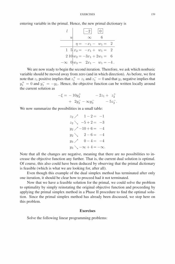
EXERCISES 159
entering variable in the primal. Hence, the new primal dictionary is
l −2 0
u ∞ 6
η = −x1 − w1 = 2
1 5 x2 = −x1 + w1 = 2
2 10 w2 =−3x1 + 2w1 = 6
−∞ 0 w3 = 2x1 − w1 =−4 .
We are now ready to begin the second iteration. Therefore, we ask which nonbasic
variable should be moved away from zero (and in which direction). As before, we first
note that z1 positive implies that z+1 = z1 and z−1 = 0 and that y1 negative implies that
y+1 = 0 and y−
1 = −y1. Hence, the objective function can be written locally around
the current solution as
−ξ = − 10y+2 − 2z1 + z+
2
+ 2y−2 −∞y−
3 − 5z−2 .
We now summarize the possibilities in a small table:
z2 ր 1− 2 = −1
z2 ց −5 + 2 = −3
y2 ր−10 + 6 = −4
y2 ց 2− 6 = −4
y3 ր 0− 4 = −4
y3 ց−∞+ 4 =−∞.
Note that all the changes are negative, meaning that there are no possibilities to in-
crease the objective function any further. That is, the current dual solution is optimal.
Of course, this also could have been deduced by observing that the primal dictionary
is feasible (which is what we are looking for, after all).
Even though this example of the dual simplex method has terminated after only
one iteration, it should be clear how to proceed had it not terminated.
Now that we have a feasible solution for the primal, we could solve the problem
to optimality by simply reinstating the original objective function and proceeding by
applying the primal simplex method in a Phase II procedure to find the optimal solu-
tion. Since the primal simplex method has already been discussed, we stop here on
this problem.
Exercises
Solve the following linear programming problems:

160 9. PROBLEMS IN GENERAL FORM
9.1 maximize −x1 + x2
subject to −x1 + x2 ≤ 5
x1 − 2x2 ≤ 9
0 ≤ x1 ≤ 6
0 ≤ x2 ≤ 8.
9.2 maximize −3x1 − x2 + x3 + 2x4 − x5 + x6 − x7 − 4x8
subject to x1 + 4x3 + x4 − 5x5 − 2x6 + 3x7 − 6x8 = 7
x2 − 3x3 − x4 + 4x5 + x6 − 2x7 + 5x8 =−3
0 ≤ x1 ≤ 8
0 ≤ x2 ≤ 6
0 ≤ x3 ≤ 10
0 ≤ x4 ≤ 15
0 ≤ x5 ≤ 2
0 ≤ x6 ≤ 10
0 ≤ x7 ≤ 4
0 ≤ x8 ≤ 3.
Notes
Dantzig (1955) was the first to consider variants of the simplex method that handle
bounds and ranges implicitly.
CHAPTER 10
Convex Analysis
This book is mostly about linear programming. However, this subject, important
as it is, is just a subset of a larger subject called convex analysis. In this chapter, we
shall give a brief introduction to this broader subject. In particular, we shall prove a
few of the fundamental results of convex analysis and see that their proofs depend on
some of the theory of linear programming that we have already developed.
1. Convex Sets
Given a finite set of points, z1, z2, . . . , zn, in Rm, a point z in R
m is called a
convex combination of these points if1
z =n
∑
j=1
tjzj ,
where tj ≥ 0 for each j and∑n
j=1 tj = 1. It is called a strict convex combination if
none of the tj’s vanish. For n = 2, the set of all convex combinations of two points is
simply the line segment connecting them.
A subset S of Rm is called convex if, for every x and y in S, S also contains all
points on the line segment connecting x and y. That is, tx + (1 − t)y ∈ S, for every
0 < t < 1. See Figure 10.1.
Certain elementary properties of convex sets are trivial to prove. For example,
the intersection of an arbitrary collection of convex sets is convex. Indeed, let Sα,
α ∈ I , denote a collection of convex sets indexed by some set I . Then the claim is
that ∩α∈ISα is convex. To see this, consider an arbitrary pair of points x and y in the
intersection. It follows that x and y are in each Sα. By the convexity of Sα it follows
that Sα contains the line segment connecting x and y. Since each of these sets contains
the line segment, so does their intersection. Hence, the intersection is convex.
Here is another easy one:
THEOREM 10.1. A set C is convex if and only if it contains all convex combina-
tions of points in C.
1Until now we’ve used subscripts for the components of a vector. In this chapter, subscripts will be
used to list sequences of vectors. Hopefully, this will cause no confusion.
161
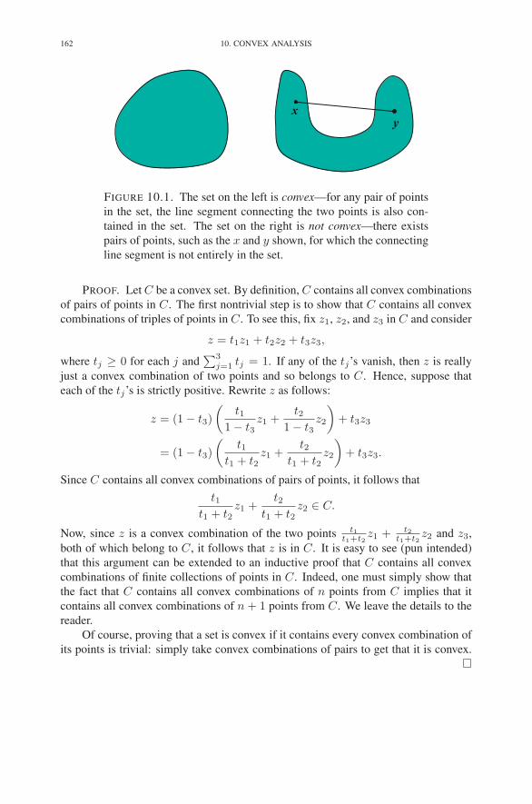
162 10. CONVEX ANALYSIS
xy
FIGURE 10.1. The set on the left is convex—for any pair of points
in the set, the line segment connecting the two points is also con-
tained in the set. The set on the right is not convex—there exists
pairs of points, such as the x and y shown, for which the connecting
line segment is not entirely in the set.
PROOF. Let C be a convex set. By definition, C contains all convex combinations
of pairs of points in C. The first nontrivial step is to show that C contains all convex
combinations of triples of points in C. To see this, fix z1, z2, and z3 in C and consider
z = t1z1 + t2z2 + t3z3,
where tj ≥ 0 for each j and∑3
j=1 tj = 1. If any of the tj’s vanish, then z is really
just a convex combination of two points and so belongs to C. Hence, suppose that
each of the tj’s is strictly positive. Rewrite z as follows:
z = (1 − t3)
(
t11 − t3
z1 +t2
1 − t3z2
)
+ t3z3
= (1 − t3)
(
t1t1 + t2
z1 +t2
t1 + t2z2
)
+ t3z3.
Since C contains all convex combinations of pairs of points, it follows that
t1t1 + t2
z1 +t2
t1 + t2z2 ∈ C.
Now, since z is a convex combination of the two points t1t1+t2
z1 + t2t1+t2
z2 and z3,
both of which belong to C, it follows that z is in C. It is easy to see (pun intended)
that this argument can be extended to an inductive proof that C contains all convex
combinations of finite collections of points in C. Indeed, one must simply show that
the fact that C contains all convex combinations of n points from C implies that it
contains all convex combinations of n + 1 points from C. We leave the details to the
reader.
Of course, proving that a set is convex if it contains every convex combination of
its points is trivial: simply take convex combinations of pairs to get that it is convex.
�

2. CARATHEODORY’S THEOREM 163
For each set S in Rm (not necessarily convex), there exists a smallest convex set,
which we shall denote by conv(S), containing S. It is defined, quite simply, as the
intersection of all convex sets containing S. From our discussion about intersections,
it follows that this set is convex. The set conv(S) is called the convex hull of S.
This definition can be thought of as a definition from the “outside,” since it involves
forming the intersection of a collection of sets that contain S. Our next theorem gives
a characterization of convex sets from the “inside”:
THEOREM 10.2. The convex hull conv(S) of a set S in Rm consists precisely of
the set of all convex combinations of finite collections of points from S.
PROOF. Let H denote the set of all convex combinations of finite sets of points
in S:
H =
⎧
⎨
⎩
z =
n∑
j=1
tjzj : n ≥ 1, zj ∈ S and tj > 0 for all j, and
n∑
j=1
tj = 1
⎫
⎬
⎭
.
It suffices to show that (1) H contains S, (2) H is convex, and (3) every convex set
containing S also contains H .
To see that H contains S, just take n = 1 in the definition of H .
To see that H is convex, fix two points x and y in H and a real number 0 < t < 1.
We must show that z = tx + (1 − t)y ∈ H . The fact that x ∈ H implies that
x =∑r
j=1 pjxj , for some r ≥ 1, where pj > 0 for j = 1, 2, . . . , r,∑r
j=1 pj = 1,
and xj ∈ S for j = 1, 2, . . . , r. Similarly, the fact that y is in H implies that y =∑s
j=1 qjyj , for some s ≥ 1, where qj > 0 for j = 1, 2, . . . , s,∑s
j=1 qj = 1, and
yj ∈ S for j = 1, 2, . . . , s. Hence,
z = tx + (1 − t)y =
r∑
j=1
tpjxj +
s∑
j=1
(1 − t)qjyj .
Since the coefficients (tp1, . . . , tpr, (1 − t)q1, . . . , (1 − t)qs) are all positive and sum
to one, it follows that this last expression for z is a convex combination of r + s points
from S. Hence, z is in H . Since x and y were arbitrary points in H and t was an
arbitrary real number between zero and one, the fact that z ∈ H implies that H is
convex.
It remains simply to show that H is contained in every convex set containing S.
Let C be such a set (i.e., convex and containing S). From Theorem 10.1 and the fact
that C contains S, it follows that C contains all convex combinations of points in S.
Hence, C contains H . �
2. Caratheodory’s Theorem
In the previous section, we showed that the convex hull of a set S can be con-
structed by forming all convex combinations of finite sets of points from S. In 1907,
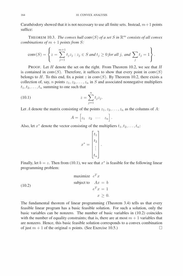
164 10. CONVEX ANALYSIS
Caratheodory showed that it is not necessary to use all finite sets. Instead, m+1 points
suffice:
THEOREM 10.3. The convex hull conv(S) of a set S in Rm consists of all convex
combinations of m + 1 points from S:
conv(S) =
⎧
⎨
⎩
z =m+1∑
j=1
tjzj : zj ∈ S and tj ≥ 0 for all j, and∑
j
tj = 1
⎫
⎬
⎭
.
PROOF. Let H denote the set on the right. From Theorem 10.2, we see that His contained in conv(S). Therefore, it suffices to show that every point in conv(S)belongs to H . To this end, fix a point z in conv(S). By Theorem 10.2, there exists a
collection of, say, n points z1, z2, . . . , zn in S and associated nonnegative multipliers
t1, t2, . . . , tn summing to one such that
(10.1) z =
n∑
j=1
tjzj .
Let A denote the matrix consisting of the points z1, z2, . . . , zn as the columns of A:
A =[
z1 z2 · · · zn
]
.
Also, let x∗ denote the vector consisting of the multipliers t1, t2, . . . , tn:
x∗ =
⎡
⎢
⎢
⎢
⎢
⎢
⎣
t1
t2...
tn
⎤
⎥
⎥
⎥
⎥
⎥
⎦
.
Finally, let b = z. Then from (10.1), we see that x∗ is feasible for the following linear
programming problem:
(10.2)
maximize cT x
subject to Ax = b
eT x = 1
x ≥ 0.
The fundamental theorem of linear programming (Theorem 3.4) tells us that every
feasible linear program has a basic feasible solution. For such a solution, only the
basic variables can be nonzero. The number of basic variables in (10.2) coincides
with the number of equality constraints; that is, there are at most m + 1 variables that
are nonzero. Hence, this basic feasible solution corresponds to a convex combination
of just m + 1 of the original n points. (See Exercise 10.5.) �

3. THE SEPARATION THEOREM 165
It is easy to see that the number m+1 is the best possible. For example, the point
(1/(m+1), 1/(m+1), . . . , 1/(m+1)) in Rm belongs to the convex hull of the m+1
points e1, e2, . . . , em, 0 but is not a convex combination of any subset of them.
3. The Separation Theorem
We shall define a halfspace of Rn to be any set given by a single (nontrivial) linear
inequality:
(10.3) {x ∈ Rn :
n∑
j=1
ajxj ≤ b}, (a1, a2, . . . , an) �= 0.
Every halfspace is convex. To see this, suppose that x = (x1, x2, . . . , xn) and y =(y1, y2, . . . , yn) both satisfy the linear inequality in (10.3). Fix t between zero and
one. Then both t and 1 − t are nonnegative, and so multiplying by them preserves the
direction of inequality. Therefore, multiplying∑
j ajxj ≤ b by t and∑
j ajyj ≤ bby 1 − t and then adding, we get
∑
j
aj (txj + (1 − t)yj) ≤ b.
That is, tx + (1 − t)y also satisfies the inequality defining the halfspace.
If we allow the vector of coefficients (a1, a2, . . . , an) in the definition of a half-
space to vanish, then we call the set so defined a generalized halfspace. It is easy to
see that every generalized halfspace is simply a halfspace, all of Rn, or the empty set.
Also, every generalized halfspace is clearly convex.
A polyhedron is defined as the intersection of a finite collection of generalized
halfspaces. That is, a polyhedron is any set of the form
{x ∈ Rn :
n∑
j=1
aijxj ≤ bi, i = 1, 2, . . . , m}.
Every polyhedron, being the intersection of a collection of convex sets, is convex.
The following theorem is called the Separation Theorem for polyhedra.
THEOREM 10.4. Let P and P be two disjoint nonempty polyhedra in Rn. Then
there exist disjoint halfspaces H and H such that P ⊂ H and P ⊂ H .
PROOF. Suppose that P and P are given by the following systems of inequalities:
P = {x : Ax ≤ b},P = {x : Ax ≤ b}.
The disjointness of P and P implies that there is no solution to the system
(10.4)
[
A
A
]
x ≤[
b
b
]
.

166 10. CONVEX ANALYSIS
To continue the proof, we need a result known as Farkas’ Lemma, which says that
Ax ≤ b has no solutions if and only if there is an m-vector y such that
AT y = 0
y ≥ 0
bT y < 0.
We shall prove this result in the next section. For now, let us apply Farkas’ Lemma to
the situation at hand. Indeed, the fact that there are no solutions to (10.4) implies that
there exists a vector, which we shall write in block form as[
y
y
]
,
such that
[
AT AT]
[
y
y
]
= AT y + AT y = 0(10.5)
[
y
y
]
≥ 0(10.6)
[
bT bT]
[
y
y
]
= bT y + bT y < 0.(10.7)
From the last condition, we see that either bT y < 0 or bT y < 0 (or both). Without
loss of generality, we may assume that
bT y < 0.
Farkas’ Lemma (this time applied in the other direction) together with the nonempti-
ness of P now implies that
AT y �= 0.
Put
H ={
x : (AT y)T x ≤ bT y}
and H ={
x : (AT y)T x ≥ −bT y}
.
These sets are clearly halfspaces. To finish the proof, we must show that they are
disjoint and contain their corresponding polyhedra.
First of all, it follows from (10.7) that H and H are disjoint. Indeed, suppose that
x ∈ H . Then (AT y)T x ≤ bT y < −bT y, which implies that x is not in H .
To show that P ⊂ H , fix x in P . Then Ax ≤ b. Since y ≥ 0 (as we know from
(10.6)), it follows then that yT Ax ≤ yT b. But this is exactly the condition that says
that x belongs to H . Since x was an arbitrary point in P , it follows that P ⊂ H .
Showing that P is a subset of H is similar. Indeed, suppose that x ∈ P . Then
Ax ≤ b. Multiplying on the left by −yT and noting that y ≥ 0, we see that −yT Ax ≥
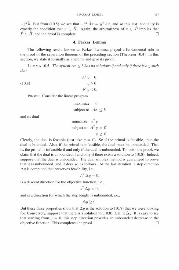
4. FARKAS’ LEMMA 167
−yT b. But from (10.5) we see that −yT Ax = yT Ax, and so this last inequality is
exactly the condition that x ∈ H . Again, the arbitrariness of x ∈ P implies that
P ⊂ H , and the proof is complete. �
4. Farkas’ Lemma
The following result, known as Farkas’ Lemma, played a fundamental role in
the proof of the separation theorem of the preceding section (Theorem 10.4). In this
section, we state it formally as a lemma and give its proof.
LEMMA 10.5. The system Ax ≤ b has no solutions if and only if there is a y such
that
AT y = 0
y ≥ 0(10.8)
bT y < 0.
PROOF. Consider the linear program
maximize 0
subject to Ax ≤ b
and its dual
minimize bT y
subject to AT y = 0
y ≥ 0.
Clearly, the dual is feasible (just take y = 0). So if the primal is feasible, then the
dual is bounded. Also, if the primal is infeasible, the dual must be unbounded. That
is, the primal is infeasible if and only if the dual is unbounded. To finish the proof, we
claim that the dual is unbounded if and only if there exists a solution to (10.8). Indeed,
suppose that the dual is unbounded. The dual simplex method is guaranteed to prove
that it is unbounded, and it does so as follows. At the last iteration, a step direction
∆y is computed that preserves feasibility, i.e.,
AT ∆y = 0,
is a descent direction for the objective function, i.e.,
bT ∆y < 0,
and is a direction for which the step length is unbounded, i.e.,
∆y ≥ 0.
But these three properties show that ∆y is the solution to (10.8) that we were looking
for. Conversely, suppose that there is a solution to (10.8). Call it ∆y. It is easy to see
that starting from y = 0, this step direction provides an unbounded decrease in the
objective function. This completes the proof. �

168 10. CONVEX ANALYSIS
5. Strict Complementarity
In this section, we consider the usual inequality-form linear programming prob-
lem, which we write with its slack variables shown explicitly:
(10.9)
maximize cT x
subject to Ax + w = b
x, w ≥ 0.
As we know, the dual can be written as follows:
(10.10)
minimize bT y
subject to AT y − z = c
y, z ≥ 0.
In our study of duality theory in Chapter 5, we saw that every pair of optimal solu-
tions to these two problems possesses a property called complementary slackness. If
(x∗, w∗) denotes an optimal solution to the primal and (y∗, z∗) denotes an optimal
solution to the dual, then the complementary slackness theorem says that, for each
j = 1, 2, . . . , n, either x∗j = 0 or z∗j = 0 (or both) and, for each i = 1, 2, . . . ,m,
either y∗i = 0 or w∗
i = 0 (or both). In this section, we shall prove that there are opti-
mal pairs of solutions for which the parenthetical “or both” statements don’t happen.
That is, there are optimal solutions for which exactly one member of each pair (x∗j , z
∗j )
vanishes and exactly one member from each pair (y∗i , w∗
i ) vanishes. In such cases, we
say that the optimal solutions are strictly complementary to each other. The strictness
of the complementary slackness is often expressed by saying that x∗ + z∗ > 0 and
y∗ + w∗ > 02.
As a warm-up, we prove the following theorem.
THEOREM 10.6. If both the primal and the dual have feasible solutions, then
there exists a primal feasible solution (x, w) and a dual feasible solution (y, z) such
that x + z > 0 and y + w > 0.
PROOF. If there is a feasible primal solution x for which xj > 0, then it doesn’t
matter whether there is a feasible dual solution whose jth slack variable is strictly
positive. But what about indices j for which xj = 0 for every feasible solution? Let jbe such an index. Consider the following linear programming problem:
(10.11)
maximize xj
subject to Ax≤ b
x≥ 0.
2Given any vector ξ, we use the notation ξ > 0 to indicate that every component of ξ is strictly
positive: ξj > 0 for all j

5. STRICT COMPLEMENTARITY 169
This problem is feasible, since its constraints are the same as for the original primal
problem (10.9). Furthermore, it has an optimal solution (the corresponding objective
function value is zero). The dual of (10.11) is:
minimize bT y
subject to AT y ≥ ej
y ≥ 0.
By the strong duality theorem, the dual has an optimal solution, say y′. Letting z′
denote the corresponding slack variable, we have that
AT y′ − z′ = ej
y′, z′ ≥ 0.
Now, let y be any feasible solution to (10.10) and let z be the corresponding slack
variable. Then the above properties of y′ and z′ imply that y + y′ is feasible for
(10.10) and its slack is z + z′ + ej . Clearly, for this dual feasible solution we have
that the jth component of its vector of slack variables is at least 1. To summarize, we
have shown that, for each j, there exists a primal feasible solution, call it (x(j), w(j)),
and a dual feasible solution, call it (y(j), z(j)), such that x(j)j + z
(j)j > 0. In the same
way, one can exhibit primal and dual feasible solutions for which each individual dual
variable and its corresponding primal slack add to a positive number. To complete the
proof, we now form a strict convex combination of these n + m feasible solutions.
Since the feasible region for a linear programming problem is convex, these convex
combinations preserve primal and dual feasibility. Since the convex combination is
strict, it follows that every primal variable and its dual slack add to a strictly positive
number as does every dual variable and its primal slack. �
A variable xj that must vanish in order for a linear programming problem to be
feasible is called a null variable. The previous theorem says that if a variable is null,
then its dual slack is not null.
The following theorem is called the Strict Complementary Slackness Theorem
THEOREM 10.7. If a linear programming problem has an optimal solution, then
there is an optimal solution (x∗, w∗) and an optimal dual solution (y∗, z∗) such that
x∗ + z∗ > 0 and y∗ + w∗ > 0.
We already know from the complementary slackness theorem (Theorem 5.1) that
x∗ and z∗ are complementary to each other as are y∗ and w∗. This theorem then
asserts that the complementary slackness is strict.
PROOF. The proof is much the same as the proof of Theorem 10.6 except this
time we look at an index j for which xj vanishes in every optimal solution. We then

170 10. CONVEX ANALYSIS
consider the following problem:
(10.12)
maximize xj
subject to Ax≤ b
cT x≥ ζ∗
x≥ 0,
where ζ∗ denotes the objective value of the optimal solution to the original problem. In
addition to the dual variables y corresponding to the Ax ≤ b constraints, there is one
more dual variable, call it t, associated with the constraint cT x ≥ ζ∗. The analysis
of problem (10.12) is similar to the analysis given in Theorem 10.6 except that one
must now consider two cases: (a) the optimal value of t is strictly positive and (b) the
optimal value of t vanishes. The details are left as an exercise (see Exercise 10.6). �
Exercises
10.1 Is Rn a polyhedron?
10.2 For each b ∈ Rm, let ξ∗(b) denote the optimal objective function value for
the following linear program:
maximize cT x
subject to Ax≤ b
x≥ 0.
Suppose that ξ∗(b) < ∞ for all b. Show that the function ξ∗(b) is concave (a
function f on Rm is called concave if f(tx+(1−t)y) ≥ tf(x)+(1−t)f(y)
for all x and y in Rm and all 0 < t < 1). Hint: Consider the dual problem.
10.3 Describe how one needs to modify the proof of Theorem 10.4 to get a proof
of the following result:
Let P and P be two disjoint polyhedra in Rn. Then there exist
disjoint generalized halfspaces H and H such that P ⊂ H and
P ⊂ H .
10.4 Find a strictly complementary solution to the following linear programming
problem and its dual:
maximize 2x1 + x2
subject to 4x1 + 2x2 ≤ 6
x2 ≤ 1
2x1 + x2 ≤ 3
x1, x2 ≥ 0.

NOTES 171
10.5 There is a slight oversimplification in the proof of Theorem 10.3. Can you
spot it? Can you fix it?
10.6 Complete the proof of Theorem 10.7.
10.7 Interior solutions. Prove the following statement: If a linear programming
problem has feasible solutions and the set of feasible solutions is bounded,
then there is a strictly positive dual feasible solution: y > 0 and z > 0.
Hint. It is easier to prove the equivalent statement: if a linear programming
problem has feasible solutions and the dual has null variables, then the set
of primal feasible solutions is an unbounded set.
Notes
Caratheodory (1907) proved Theorem 10.3. Farkas (1902) proved Lemma 10.5.
Several similar results were discovered by many others, including Gordan (1873),
Stiemke (1915), Ville (1938), and Tucker (1956). The standard reference on convex
analysis is Rockafellar (1970).


CHAPTER 11
Game Theory
In this chapter, we shall study if not the most practical then certainly an elegant
application of linear programming. The subject is called game theory, and we shall
focus on the simplest type of game, called the finite two-person zero-sum game, or
just matrix game for short. Our primary goal shall be to prove the famous Minimax
Theorem, which was first discovered and proved by John von Neumann in 1928. His
original proof of this theorem was rather involved and depended on another beautiful
theorem from mathematics, the Brouwer Fixed-Point Theorem. However, it eventu-
ally became clear that the solution of matrix games could be found by solving a certain
linear programming problem and that the Minimax Theorem is just a fairly straight-
forward consequence of the Duality Theorem.
1. Matrix Games
A matrix game is a two-person game defined as follows. Each person first selects,
independently of the other, an action from a finite set of choices (the two players in
general will be confronted with different sets of actions from which to choose). Then
both reveal to each other their choice. If we let i denote the first player’s choice and
j denote the second player’s choice, then the rules of the game stipulate that the first
player will pay the second player aij dollars. The array of possible payments
A = [aij ]
is presumed known to both players before the game begins. Of course, if aij is negative
for some pair (i, j), then the payment goes in the reverse direction — from the second
player to the first. For obvious reasons, we shall refer to the first player as the row
player and the second player as the column player. Since we have assumed that the
row player has only a finite number of actions from which to choose, we can enumerate
these actions and assume without loss of generality that i is simply an integer selected
from 1 to m. Similarly, we can assume that j is simply an index ranging from 1to n (in its real-world interpretation, row action 3 will generally have nothing to do
with column action 3—the number 3 simply indicates that it is the third action in the
enumerated list of choices).
Let us look at a specific familiar example. Namely, consider the game every
child knows, called Paper–Scissors–Rock. To refresh the memory of older readers,
173
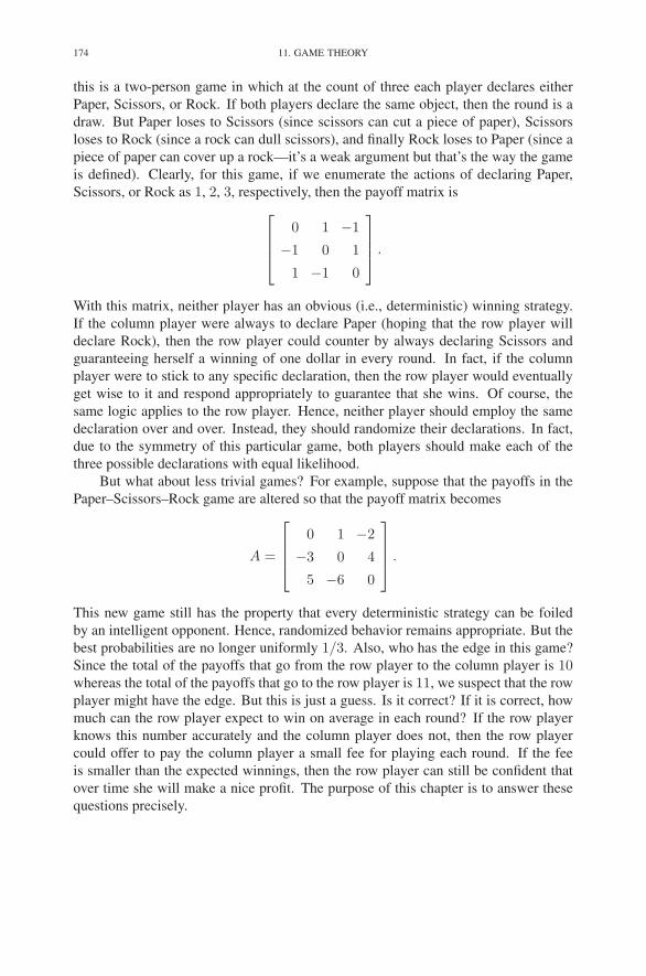
174 11. GAME THEORY
this is a two-person game in which at the count of three each player declares either
Paper, Scissors, or Rock. If both players declare the same object, then the round is a
draw. But Paper loses to Scissors (since scissors can cut a piece of paper), Scissors
loses to Rock (since a rock can dull scissors), and finally Rock loses to Paper (since a
piece of paper can cover up a rock—it’s a weak argument but that’s the way the game
is defined). Clearly, for this game, if we enumerate the actions of declaring Paper,
Scissors, or Rock as 1, 2, 3, respectively, then the payoff matrix is
⎡
⎢
⎢
⎣
0 1 −1
−1 0 1
1 −1 0
⎤
⎥
⎥
⎦
.
With this matrix, neither player has an obvious (i.e., deterministic) winning strategy.
If the column player were always to declare Paper (hoping that the row player will
declare Rock), then the row player could counter by always declaring Scissors and
guaranteeing herself a winning of one dollar in every round. In fact, if the column
player were to stick to any specific declaration, then the row player would eventually
get wise to it and respond appropriately to guarantee that she wins. Of course, the
same logic applies to the row player. Hence, neither player should employ the same
declaration over and over. Instead, they should randomize their declarations. In fact,
due to the symmetry of this particular game, both players should make each of the
three possible declarations with equal likelihood.
But what about less trivial games? For example, suppose that the payoffs in the
Paper–Scissors–Rock game are altered so that the payoff matrix becomes
A =
⎡
⎢
⎢
⎣
0 1 −2
−3 0 4
5 −6 0
⎤
⎥
⎥
⎦
.
This new game still has the property that every deterministic strategy can be foiled
by an intelligent opponent. Hence, randomized behavior remains appropriate. But the
best probabilities are no longer uniformly 1/3. Also, who has the edge in this game?
Since the total of the payoffs that go from the row player to the column player is 10whereas the total of the payoffs that go to the row player is 11, we suspect that the row
player might have the edge. But this is just a guess. Is it correct? If it is correct, how
much can the row player expect to win on average in each round? If the row player
knows this number accurately and the column player does not, then the row player
could offer to pay the column player a small fee for playing each round. If the fee
is smaller than the expected winnings, then the row player can still be confident that
over time she will make a nice profit. The purpose of this chapter is to answer these
questions precisely.
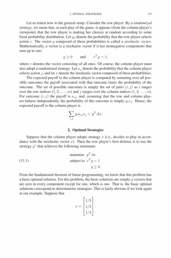
2. OPTIMAL STRATEGIES 175
Let us return now to the general setup. Consider the row player. By a randomized
strategy, we mean that, at each play of the game, it appears (from the column player’s
viewpoint) that the row player is making her choices at random according to some
fixed probability distribution. Let yi denote the probability that the row player selects
action i. The vector y composed of these probabilities is called a stochastic vector.
Mathematically, a vector is a stochastic vector if it has nonnegative components that
sum up to one:
y ≥ 0 and eT y = 1,
where e denotes the vector consisting of all ones. Of course, the column player must
also adopt a randomized strategy. Let xj denote the probability that the column player
selects action j, and let x denote the stochastic vector composed of these probabilities.
The expected payoff to the column player is computed by summing over all pos-
sible outcomes the payoff associated with that outcome times the probability of the
outcome. The set of possible outcomes is simply the set of pairs (i, j) as i ranges
over the row indices (1, 2, . . . , m) and j ranges over the column indices (1, 2, . . . , n).
For outcome (i, j) the payoff is aij , and, assuming that the row and column play-
ers behave independently, the probability of this outcome is simply yixj . Hence, the
expected payoff to the column player is
∑
i,j
yiaijxj = yT Ax.
2. Optimal Strategies
Suppose that the column player adopts strategy x (i.e., decides to play in accor-
dance with the stochastic vector x). Then the row player’s best defense is to use the
strategy y∗ that achieves the following minimum:
(11.1)
minimize yT Ax
subject to eT y = 1
y ≥ 0.
From the fundamental theorem of linear programming, we know that this problem has
a basic optimal solution. For this problem, the basic solutions are simply y vectors that
are zero in every component except for one, which is one. That is, the basic optimal
solutions correspond to deterministic strategies. This is fairly obvious if we look again
at our example. Suppose that
x =
⎡
⎢
⎢
⎣
1/3
1/3
1/3
⎤
⎥
⎥
⎦
.

176 11. GAME THEORY
Then
Ax =
⎡
⎢
⎢
⎣
−1/3
1/3
−1/3
⎤
⎥
⎥
⎦
,
and so the row player’s best choice is to select either i = 1 (Paper) or i = 3 (Rock)
or any combination thereof. That is, an optimal solution is y∗ = (1, 0, 0) (it is not
unique).
Since for any given x the row player will adopt the strategy that achieves the
minimum in (11.1), it follows that the column player should employ a strategy x∗ that
attains the following maximum:
(11.2) maxx
miny
yT Ax,
where the max and the min are over all stochastic vectors (of the appropriate dimen-
sion).
The question then becomes: how do we solve (11.2)? It turns out that this problem
can be reformulated as a linear programming problem. Indeed, we have already seen
that the inner optimization (the minimization) can be taken over just the deterministic
strategies:
miny
yT Ax = mini
eTi Ax,
where we have used ei to denote the vector of all zeros except for a one in position i.Hence, the max-min problem given in (11.2) can be rewritten as
maximize(
mini eTi Ax
)
subject to
n∑
j=1
xj = 1
xj ≥ 0 j = 1, 2, . . . , n.
Now, if we introduce a new variable, v, representing a lower bound on the eTi Ax’s,
then we see that the problem can be recast as a linear program:
maximize v
subject to v ≤ eTi Ax i = 1, 2, . . . , m
n∑
j=1
xj = 1
xj ≥ 0 j = 1, 2, . . . , n.

3. THE MINIMAX THEOREM 177
Switching back to vector notation, the problem can be written as
maximize v
subject to ve − Ax≤ 0
eT x = 1
x≥ 0.
Finally, writing in block-matrix form, we get
(11.3)
maximize[
0 1]
[
x
v
]
subject to
[
−A e
eT 0
][
x
v
]
≤=
[
0
1
]
x≥ 0
v free.
Now let’s turn it around. By symmetry, the row player seeks a strategy y∗ that
attains optimality in the following min-max problem:
miny
maxx
yT Ax,
which can be reformulated as the following linear program:
minimize u
subject to ue − AT y ≥ 0
eT y = 1
y ≥ 0.
Writing in block-matrix form, we get
(11.4)
minimize[
0 1]
[
y
u
]
subject to
[
−AT e
eT 0
][
y
u
]
≥=
[
0
1
]
y ≥ 0
u free.
3. The Minimax Theorem
Having reduced the computation of the optimal strategies x∗ and y∗ to the solution
of linear programs, it is now a simple matter to show that they are consistent with each
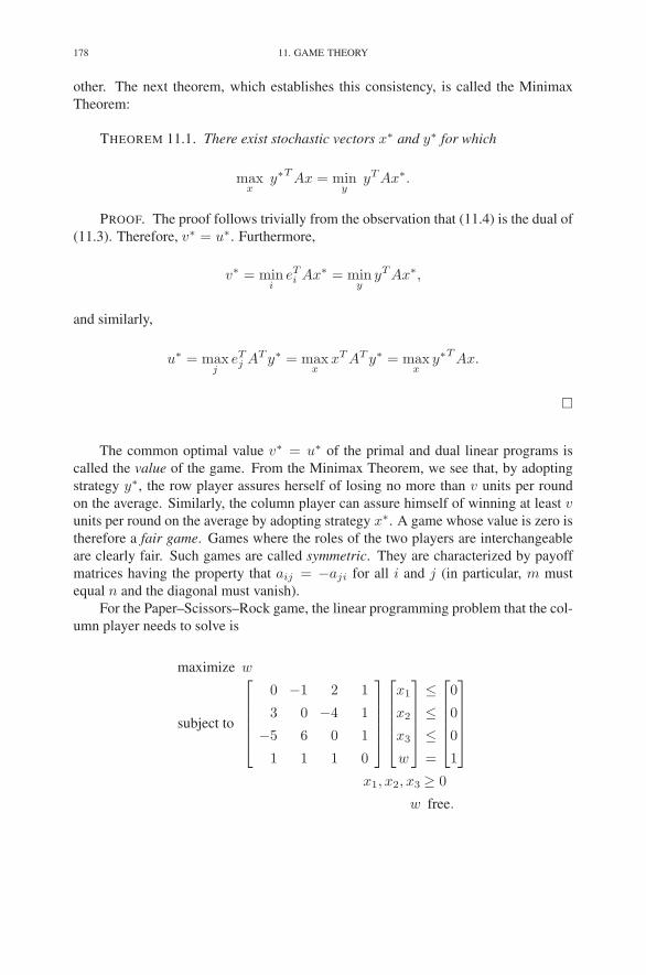
178 11. GAME THEORY
other. The next theorem, which establishes this consistency, is called the Minimax
Theorem:
THEOREM 11.1. There exist stochastic vectors x∗ and y∗ for which
maxx
y∗T Ax = miny
yT Ax∗.
PROOF. The proof follows trivially from the observation that (11.4) is the dual of
(11.3). Therefore, v∗ = u∗. Furthermore,
v∗ = mini
eTi Ax∗ = min
yyT Ax∗,
and similarly,
u∗ = maxj
eTj AT y∗ = max
xxT AT y∗ = max
xy∗T Ax.
�
The common optimal value v∗ = u∗ of the primal and dual linear programs is
called the value of the game. From the Minimax Theorem, we see that, by adopting
strategy y∗, the row player assures herself of losing no more than v units per round
on the average. Similarly, the column player can assure himself of winning at least vunits per round on the average by adopting strategy x∗. A game whose value is zero is
therefore a fair game. Games where the roles of the two players are interchangeable
are clearly fair. Such games are called symmetric. They are characterized by payoff
matrices having the property that aij = −aji for all i and j (in particular, m must
equal n and the diagonal must vanish).
For the Paper–Scissors–Rock game, the linear programming problem that the col-
umn player needs to solve is
maximize w
subject to
⎡
⎢
⎢
⎢
⎢
⎣
0 −1 2 1
3 0 −4 1
−5 6 0 1
1 1 1 0
⎤
⎥
⎥
⎥
⎥
⎦
⎡
⎢
⎢
⎢
⎢
⎣
x1
x2
x3
w
⎤
⎥
⎥
⎥
⎥
⎦
≤≤≤=
⎡
⎢
⎢
⎢
⎢
⎣
0
0
0
1
⎤
⎥
⎥
⎥
⎥
⎦
x1, x2, x3 ≥ 0
w free.

3. THE MINIMAX THEOREM 179
In nonmatrix notation, it looks like this:
maximize w
subject to −x2 + 2x3 + w ≤ 0
3x1 − 4x3 + w ≤ 0
−5x1 + 6x2 + w ≤ 0
x1 + x2 + x3 = 1
x1, x2, x3 ≥ 0.
This linear programming problem deviates from our standard inequality form in two
respects: (1) it has an equality constraint and (2) it has a free variable. There are
several ways in which one can convert this problem into standard form. The most
compact conversion is as follows. First, use the equality constraint to solve explicitly
for one of the xj’s, say x3:
x3 = 1 − x1 − x2.
Then eliminate this variable from the remaining equations to get
maximize w
subject to −2x1 − 3x2 + w ≤−2
7x1 + 4x2 + w ≤ 4
−5x1 + 6x2 + w ≤ 0
x1 + x2 ≤ 1
x1, x2 ≥ 0.
The elimination of x3 has changed the last constraint from an equality into an inequal-
ity.
The next step is to write down a starting dictionary. To do this, we need to in-
troduce slack variables for each of these constraints. It is natural (and desirable) to
denote the slack variable for the last constraint by x3. In fact, doing this, we get the
following starting dictionary:
ξ = w
x4 =−2 + 2x1 + 3x2 −w
x5 = 4− 7x1 − 4x2 −w
x6 = 5x1 − 6x2 −w
x3 = 1− x1 − x2 .
The variable w is not constrained to be nonnegative. Therefore, there is no reason for
it to be nonbasic. Let us do an arbitrary pivot with w as the entering variable and any
basic variable as the leaving variable (well, not exactly any—we must make sure that

180 11. GAME THEORY
it causes no division by 0, so therefore x3 is not a candidate). Picking x4 to leave, we
get
ξ =−2 + 2x1 + 3x2 − x4
w =−2 + 2x1 + 3x2 − x4
x5 = 6− 9x1 − 7x2 + x4
x6 = 2 + 3x1 − 9x2 + x4
x3 = 1− x1 − x2 .
Since w is free of sign constraints, it will never leave the basis (since a leaving vari-
able is, by definition, a variable that hits its lower bound—w has no such bound).
Therefore, we may as well remove it from the dictionary altogether; it can always be
computed at the end. Hence, we note that
w = −2 + 2x1 + 3x2 − x4,
or better yet that
w = ξ,
and the dictionary now becomes
ξ =−2 + 2x1 + 3x2 − x4
x5 = 6− 9x1 − 7x2 + x4
x6 = 2 + 3x1 − 9x2 + x4
x3 = 1− x1 − x2 .
At last, we are in a position to apply the simplex method. Two (tedious) iterations bring
us to the optimal dictionary. Since it involves fractions, we multiply each equation by
an integer to make each number in the dictionary an integer. Indeed, after multiplying
by 102, the optimal dictionary is given by
102ξ =−16− 27x5 − 13x6 − 62x4
102x1 = 40− 9x5 + 7x6 + 2x4
102x2 = 36− 3x5 − 9x6 + 12x4
102x3 = 26 + 12x5 + 2x6 − 14x4.
From this dictionary, it is easy to read off the optimal primal solution:
x∗ =
⎡
⎢
⎢
⎣
40/102
36/102
26/102
⎤
⎥
⎥
⎦
.

4. POKER 181
Also, since x4, x5, and x6 are complementary to y1, y2, and y3 in the dual problem,
the optimal dual solution is
y∗ =
⎡
⎢
⎢
⎣
62/102
27/102
13/102
⎤
⎥
⎥
⎦
.
Finally, the value of the game is
w∗ = ξ∗ = −16/102 = −0.15686275,
which indicates that the row player does indeed have an advantage and can expect to
make on the average close to 16 cents per round.
4. Poker
Some card games such as poker involve a round of bidding in which the players at
times bluff by increasing their bid in an attempt to coerce their opponents into backing
down, even though if the challenge is accepted they will surely lose. Similarly, they
will sometimes underbid to give their opponents false hope. In this section, we shall
study a simplified version of poker (the real game is too hard to analyze) to see if
bluffing and underbidding are justified bidding strategies.
Simplified poker involves two players, A and B, and a deck having three cards, 1,
2, and 3. At the beginning of a round, each player “antes up” $1 and is dealt one card
from the deck. A bidding session follows in which each player in turn, starting with
A, either (a) bets and adds $1 to the “kitty” or (b) passes. Bidding terminates when
a bet is followed by a bet,
a pass is followed by a pass, or
a bet is followed by a pass.
In the first two cases, the winner of the round is decided by comparing cards, and the
kitty goes to the player with the higher card. In the third case, bet followed by pass,
the player who bet wins the round independently of who had the higher card (in real
poker, the player who passes is said to fold).
With these simplified betting rules, there are only five possible betting scenarios:
A passes, B passes: $1 to holder of higher card
A passes, B bets, A passes: $1 to B
A passes, B bets, A bets: $2 to holder of higher card
A bets, B passes: $1 to A
A bets, B bets: $2 to holder of higher card

182 11. GAME THEORY
After being dealt a card, player A will decide to bet along one of three lines:
1. Pass. If B bets, pass again.
2. Pass. If B bets, bet.
3. Bet.
Similarly, after being dealt a card, player B can bet along one of four lines:
1. Pass no matter what.
2. If A passes, pass, but if A bets, bet.
3. If A passes, bet, but if A bets, pass.
4. Bet no matter what.
To model the situation as a matrix game, we must identify each player’s pure strategies.
A pure strategy is a statement of what line of betting a player intends to follow for
each possible card that the player is dealt. Hence, the players’ pure strategies can be
denoted by triples (y1, y2, y3), where yi is the line of betting that the player will use
when holding card i. (For player A, the yi’s can take values 1, 2, and 3, whereas for
player B, they can take values 1, 2, 3, and 4.)
Given a pure strategy for both players, one can compute the average payment
from, say, A to B. For example, suppose that player A adopts strategy (3, 1, 2) and
player B adopts strategy (3, 2, 4). There are six ways in which the cards can be dealt,
and we can analyze each of them as follows:
card dealt betting session payment
A B A to B
1 2 A bets, B bets 2
1 3 A bets, B bets 2
2 1 A passes, B bets, A passes 1
2 3 A passes, B bets, A passes 1
3 1 A passes, B bets, A bets −2
3 2 A passes, B passes −1
Since each of the six deals are equally likely, the average payment from A to B is
(2 + 2 + 1 + 1 − 2 − 1)/6 = 0.5The calculation of the average payment must be carried out for every combination
of pairs of strategies. How many are there? Player A has 3×3×3 = 27 pure strategies
and player B has 4×4×4 = 64 pure strategies. Hence, there are 27×64 = 1728 pairs.

4. POKER 183
Calculating the average payment for all these pairs is a daunting task. Fortunately, we
can reduce the number of pure strategies (and hence the number of pairs) that need to
be considered by making a few simple observations.
The first observation is that a player holding a 1 should never answer a bet with
a bet, since the player will lose regardless of the answering bet and will lose less by
passing. This logic implies that, when holding a 1,
player A should refrain from betting along line 2;
player B should refrain from betting along lines 2 and 4.
More clearly improvable strategies can be ruled out when holding the highest
card. For example, a player holding a 3 should never answer a bet with a pass, since
by passing the player will lose, but by betting the player will win. Furthermore, when
holding a 3, a player should always answer a pass with a bet, since in either case the
player is going to win, but answering with a bet opens the possibility of the opponent
betting again and thereby increasing the size of the win for the player holding the 3.
Hence, when holding a 3,
player A should refrain from betting along line 1;
player B should refrain from betting along lines 1, 2, and 3.
Eliminating from consideration the above lines of betting, we see that player A
now has 2×3×2 = 12 pure strategies and player B has 2×4×1 = 8 pure strategies.
The number of pairs has therefore dropped to 96—a significant reduction. Not only do
we eliminate these “bad” strategies from the mathematical model but also we assume
that both players know that these bad strategies will not be used. That is, player A
can assume that player B will play intelligently, and player B can assume the same of
A. This knowledge then leads to further reductions. For example, when holding a 2,
player A should refrain from betting along line 3. To reach this conclusion, we must
carefully enumerate possibilities. Since player A holds the 2, player B holds either the
1 or the 3. But we’ve already determined what player B will do in both of those cases.
Using this knowledge, it is not hard to see that player A would be unwise to bet along
line 3. A similar analysis reveals that, when holding a 2, player B should refrain from
lines 3 and 4. Therefore, player A now has only 2 × 2 × 2 = 8 pure strategies and
player B has only 2 × 2 × 1 = 4 pure strategies.
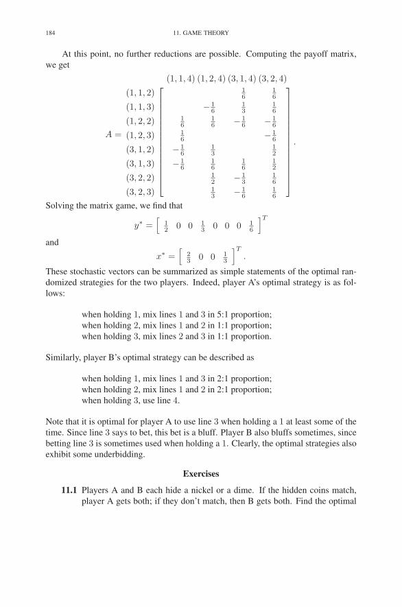
184 11. GAME THEORY
At this point, no further reductions are possible. Computing the payoff matrix,
we get
A =
(1, 1, 4) (1, 2, 4) (3, 1, 4) (3, 2, 4)
(1, 1, 2)
(1, 1, 3)
(1, 2, 2)
(1, 2, 3)
(3, 1, 2)
(3, 1, 3)
(3, 2, 2)
(3, 2, 3)
⎡
⎢
⎢
⎢
⎢
⎢
⎢
⎢
⎢
⎢
⎢
⎢
⎢
⎢
⎢
⎣
16
16
− 16
13
16
16
16 − 1
6 − 16
16 − 1
6
− 16
13
12
− 16
16
16
12
12 − 1
316
13 − 1
616
⎤
⎥
⎥
⎥
⎥
⎥
⎥
⎥
⎥
⎥
⎥
⎥
⎥
⎥
⎥
⎦
.
Solving the matrix game, we find that
y∗ =[
12 0 0 1
3 0 0 0 16
]T
and
x∗ =[
23 0 0 1
3
]T
.
These stochastic vectors can be summarized as simple statements of the optimal ran-
domized strategies for the two players. Indeed, player A’s optimal strategy is as fol-
lows:
when holding 1, mix lines 1 and 3 in 5:1 proportion;
when holding 2, mix lines 1 and 2 in 1:1 proportion;
when holding 3, mix lines 2 and 3 in 1:1 proportion.
Similarly, player B’s optimal strategy can be described as
when holding 1, mix lines 1 and 3 in 2:1 proportion;
when holding 2, mix lines 1 and 2 in 2:1 proportion;
when holding 3, use line 4.
Note that it is optimal for player A to use line 3 when holding a 1 at least some of the
time. Since line 3 says to bet, this bet is a bluff. Player B also bluffs sometimes, since
betting line 3 is sometimes used when holding a 1. Clearly, the optimal strategies also
exhibit some underbidding.
Exercises
11.1 Players A and B each hide a nickel or a dime. If the hidden coins match,
player A gets both; if they don’t match, then B gets both. Find the optimal
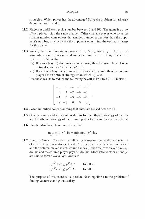
EXERCISES 185
strategies. Which player has the advantage? Solve the problem for arbitrary
denominations a and b.
11.2 Players A and B each pick a number between 1 and 100. The game is a draw
if both players pick the same number. Otherwise, the player who picks the
smaller number wins unless that smaller number is one less than the oppo-
nent’s number, in which case the opponent wins. Find the optimal strategy
for this game.
11.3 We say that row r dominates row s if arj ≥ asj for all j = 1, 2, . . . , n.
Similarly, column r is said to dominate column s if air ≥ ais for all i =1, 2, . . . ,m. Show that
(a) If a row (say, r) dominates another row, then the row player has an
optimal strategy y∗ in which y∗r = 0.
(b) If a column (say, s) is dominated by another column, then the column
player has an optimal strategy x∗ in which x∗s = 0.
Use these results to reduce the following payoff matrix to a 2 × 2 matrix:
⎡
⎢
⎢
⎢
⎢
⎣
−6 2 −4 −7 −5
0 4 −2 −9 −1
−7 3 −3 −8 −2
2 −3 6 0 3
⎤
⎥
⎥
⎥
⎥
⎦
.
11.4 Solve simplified poker assuming that antes are $2 and bets are $1.
11.5 Give necessary and sufficient conditions for the rth pure strategy of the row
and the sth pure strategy of the column player to be simultaneously optimal.
11.6 Use the Minimax Theorem to show that
maxx
miny
yT Ax = miny
maxx
yT Ax.
11.7 Bimatrix Games. Consider the following two-person game defined in terms
of a pair of m × n matrices A and B: if the row player selects row index iand the column player selects column index j, then the row player pays aij
dollars and the column player pays bij dollars. Stochastic vectors x∗ and y∗
are said to form a Nash equilibrium if
y∗T Ax∗ ≤ yT Ax∗ for all y
y∗T Bx∗ ≤ y∗T Bx for all x.
The purpose of this exercise is to relate Nash equilibria to the problem of
finding vectors x and y that satisfy
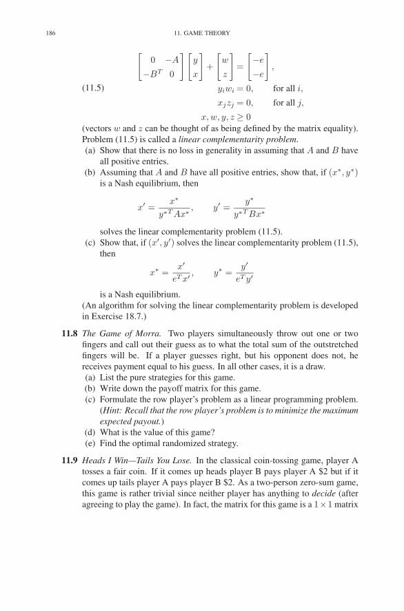
186 11. GAME THEORY
(11.5)
[
0 −A
−BT 0
][
y
x
]
+
[
w
z
]
=
[
−e
−e
]
,
yiwi = 0, for all i,
xjzj = 0, for all j,
x, w, y, z ≥ 0(vectors w and z can be thought of as being defined by the matrix equality).
Problem (11.5) is called a linear complementarity problem.
(a) Show that there is no loss in generality in assuming that A and B have
all positive entries.
(b) Assuming that A and B have all positive entries, show that, if (x∗, y∗)is a Nash equilibrium, then
x′ =x∗
y∗T Ax∗ , y′ =y∗
y∗T Bx∗
solves the linear complementarity problem (11.5).
(c) Show that, if (x′, y′) solves the linear complementarity problem (11.5),
then
x∗ =x′
eT x′ , y∗ =y′
eT y′
is a Nash equilibrium.
(An algorithm for solving the linear complementarity problem is developed
in Exercise 18.7.)
11.8 The Game of Morra. Two players simultaneously throw out one or two
fingers and call out their guess as to what the total sum of the outstretched
fingers will be. If a player guesses right, but his opponent does not, he
receives payment equal to his guess. In all other cases, it is a draw.
(a) List the pure strategies for this game.
(b) Write down the payoff matrix for this game.
(c) Formulate the row player’s problem as a linear programming problem.
(Hint: Recall that the row player’s problem is to minimize the maximum
expected payout.)
(d) What is the value of this game?
(e) Find the optimal randomized strategy.
11.9 Heads I Win—Tails You Lose. In the classical coin-tossing game, player A
tosses a fair coin. If it comes up heads player B pays player A $2 but if it
comes up tails player A pays player B $2. As a two-person zero-sum game,
this game is rather trivial since neither player has anything to decide (after
agreeing to play the game). In fact, the matrix for this game is a 1×1 matrix

NOTES 187
with only a zero in it, which represents the expected payoff from player A
to B.
Now consider the same game with the following twist. Player A is
allowed to peek at the outcome and then decide either to stay in the game
or to bow out. If player A bows out, then he automatically loses but only
has to pay player B $1. Of course, player A must inform player B of his
decision. If his decision is to stay in the game, then player B has the option
either to stay in the game or not. If she decides to get out, then she loses
$1 to player A. If both players stay in the game, then the rules are as in the
classical game: heads means player A wins, tails means player B wins.
(a) List the strategies for each player in this game. (Hint: Don’t forget that
a strategy is something that a player has control over.)
(b) Write down the payoff matrix.
(c) A few of player A’s strategies are uniformly inferior to others. These
strategies can be ruled out. Which of player A’s strategies can be ruled
out?
(d) Formulate the row player’s problem as a linear programming problem.
(Hints: (1) Recall that the row player’s problem is to minimize the max-
imum expected payout. (2) Don’t include rows that you ruled out in the
previous part.)
(e) Find the optimal randomized strategy.
(f) Discuss whether this game is interesting or not.
Notes
The Minimax Theorem was proved by von Neumann (1928). Important refer-
ences include Gale et al. (1951), von Neumann & Morgenstern (1947), Karlin (1959),
and Dresher (1961). Simplified poker was invented and analyzed by Kuhn (1950).
Exercises 11.1 and 11.2 are borrowed from Chvatal (1983).

CHAPTER 12
Regression
In this chapter, we shall study an application of linear programming to an area
of statistics called regression. As a specific example, we shall use size and iteration-
count data collected from a standard suite of linear programming problems to derive
a regression estimate of the number of iterations needed to solve problems of a given
size.
1. Measures of Mediocrity
We begin our discussion with an example. Here are the midterm exam scores for
a linear programming course:
28, 62, 80, 84, 86, 86, 92, 95, 98.
Let m denote the number of exam scores (i.e., m = 9) and let bi, i = 1, 2, . . . ,m, de-
note the actual scores (arranged in increasing order as above). The most naive measure
of the “average” score is just the mean value, x, defined by
x =1
m
m∑
i=1
bi = 79.0.
This is an example of a statistic, which, by definition, is a function of a set of data.
Statistics are computed so that one does not need to bother with reporting large tables
of raw numbers. (Admittedly, the task of reporting the above list of 9 exam scores is
not very onerous, but this is just an example.) Now, suppose the professor in question
did not report the scores but instead just gave summary statistics. Consider the student
who got an 80 on the exam. This student surely didn’t feel great about this score but
might have thought that at least it was better than average. However, as the raw data
makes clear, this student really did worse than average1 on the exam (the professor
confesses that the exam was rather easy). In fact, out of the nine students, the one
who got an 80 scored third from the bottom of the class. Furthermore, the student who
scored worst on the exam did so badly that one might expect this student to drop the
course, thereby making the 80 look even worse.
1“Average” is usually taken as synonymous with “mean” but in this section we shall use it in an
imprecise sense, employing other technically defined terms for specific meanings.
189

190 12. REGRESSION
FIGURE 12.1. The objective function whose minimum occurs at
the median.
Any statistician would, of course, immediately suggest that we report the median
score instead of the mean. The median score is, by definition, that score which is
worse than half of the other scores and better than the other half. In other words, the
median x is defined as
x = b(m+1)/2 = 86.
(Here and in various places in this chapter, we shall assume that m is odd so that
certain formulas such as this one remain fairly simple.) Clearly, the 86 gives a more
accurate indication of what the average score on the exam was.
There is a close connection between these statistical concepts and optimization.
For example, the mean x minimizes, over all real numbers x, the sum of the squared
deviations between the data points and x itself. That is,
x = argminx∈R
m∑
i=1
(x − bi)2.
To verify this claim, we let f(x) =∑m
i=1(x−bi)2, differentiate with respect to x, and
set the derivative to zero to get
f ′(x) =m∑
i=1
2(x − bi) = 0.

2. MULTIDIMENSIONAL MEASURES: REGRESSION ANALYSIS 191
Solving this equation for the critical point2 x, we see that
x =1
m
m∑
i=1
bi = x.
The fact that this critical point is a minimum rather than a maximum (or a saddle point)
follows from the fact that f ′′(x) > 0 for all x ∈ R.
The median x also enjoys a close connection with optimization. Indeed, it is the
point that minimizes the sum of the absolute values of the difference between each
data point and itself. That is,
x = argminx∈R
m∑
i=1
|x − bi|.
To see that this is correct, we again use calculus. Let
f(x) =
m∑
i=1
|x − bi|.
This function is continuous, piecewise linear, and convex (see Figure 12.1). How-
ever, it is not differentiable at the data points. Nonetheless, we can look at its de-
rivative at other points to see where it jumps across zero. The derivative, for x �∈{b1, b2, . . . , bm}, is
f ′(x) =
m∑
i=1
sgn(x − bi),
where
sgn(x) =
⎧
⎪
⎪
⎨
⎪
⎪
⎩
1 if x > 0
0 if x = 0
−1 if x < 0.
Hence, we see that the derivative at x is just the number of data points to the left of xminus the number of data points to the right. Clearly, this derivative jumps across zero
at the median, implying that the median is the minimum.
In this chapter, we shall discuss certain generalizations of means and medians
called regressions. At the end, we will consider a specific example that is of particular
interest to us: the empirical average performance of the simplex method.
2. Multidimensional Measures: Regression Analysis
The analysis of the previous section can be recast as follows. Given a “random”
observation b, we assume that it consists of two parts: a fixed, but unknown, part
2Recall from calculus that a critical point is any point at which the derivative vanishes or fails to exist.

192 12. REGRESSION
denoted by x and a random fluctuation about this fixed part, which we denote by ǫ.
Hence,
b = x + ǫ.
Now, if we take several observations and index them as i = 1, 2, . . . ,m, the b’s and
the ǫ’s will vary, but x is assumed to be the same for all observations. Therefore, we
can summarize the situation by writing
bi = x + ǫi, i = 1, 2, . . . , m.
We now see that the mean is simply the value of x that minimizes the sum of the
squares of the ǫi’is. Similarly, the median is the value of x that minimizes the sum of
the absolute values of the ǫi’s.
Sometimes one wishes to do more than merely identify some sort of “average.”
For example, a medical researcher might collect blood pressure data on thousands
of patients with the aim of identifying how blood pressure depends on age, obesity
(defined as weight over height), sex, etc. So associated with each observation b of
a blood pressure are values of these control variables. Let’s denote by a1 the age
of a person, a2 the obesity, a3 the sex, etc. Let n denote the number of different
control variables being considered by the researcher. In (linear) regression analysis,
we assume that the response b depends linearly on the control variables. Hence, we
assume that there are (unknown) numbers xj , j = 1, 2, . . . , n, such that
b =
n∑
j=1
ajxj + ǫ.
This equation is referred to as the regression model. Of course, the researcher collects
data from thousands of patients, and so the data items, b and the aj’s, must be indexed
over these patients. That is,
bi =
n∑
j=1
aijxj + ǫi, i = 1, 2, . . . ,m.
If we let b denote the vector of observations, ǫ the vector of random fluctuations, and
A the matrix whose ith row consists of the values of the control variables for the ithpatient, then the regression model can be expressed in matrix notation as
(12.1) b = Ax + ǫ.
In regression analysis, the goal is to find the vector x that best explains the obser-
vations b. Hence, we wish to pick values that minimize, in some sense, the vector ǫ’s.
Just as for the mean and median, we can consider minimizing either the sum of the
squares of the ǫi’s or the sum of the absolute values of the ǫi’s. There are even other
possibilities. In the next two sections, we will discuss the range of possibilities and
then give specifics for the two mentioned above.
3. L2-REGRESSION 193
3. L2-Regression
There are several notions of the size of a vector. The most familiar one is the
Euclidean length
‖y‖2 = (∑
i
y2i )1/2.
This notion of length corresponds to our physical notion (at least when the dimension
is low, such as 1, 2, or 3). However, one can use any power inside the sum as long as
the corresponding root accompanies it on the outside of the sum. For 1 ≤ p < ∞, we
get then the so-called Lp-norm of a vector y
‖y‖p = (∑
i
ypi )1/p.
Other than p = 2, the second most important case is p = 1 (and the third most
important case corresponds to the limit as p tends to infinity).
Measuring the size of ǫ in (12.1) using the L2-norm, we arrive at the L2-regression
problem, which is to find x that attains the minimum L2-norm for the difference be-
tween b and Ax. Of course, it is entirely equivalent to minimize the square of the
L2-norm, and so we get
x = argminx‖b − Ax‖22.
Just as for the mean, there is an explicit formula for x. To find it, we again rely on
elementary calculus. Indeed, let
f(x) = ‖b − Ax‖22 =
∑
i
⎛
⎝bi −∑
j
aijxj
⎞
⎠
2
.
In this multidimensional setting, a critical point is defined as a point at which the
derivative with respect to every variable vanishes. So if we denote a critical point by
x, we see that it must satisfy the following equations:
∂f
∂xk(x) =
∑
i
2
⎛
⎝bi −∑
j
aij xj
⎞
⎠ (−aik) = 0, k = 1, 2, . . . , n.
Simplifying these equations, we get∑
i
aikbi =∑
i
∑
j
aikaij xj , k = 1, 2, . . . , n.
In matrix notation, these equations can be summarized as follows:
AT b = AT Ax.
In other words, assuming that AT A is invertible, we get
(12.2) x = (AT A)−1AT b.

194 12. REGRESSION
a
b
0 1 2 3 40
1
2
3
4
FIGURE 12.2. Three data points for a linear regression.
This is the formula for L2-regression. It is also commonly called least squares regres-
sion. In Section 12.6, we will use this formula to solve a specific regression problem.
Example. The simplest and most common regression model arises when one
wishes to describe a response variable b as a linear function of a single input vari-
able a. In this case, the model is
b = ax1 + x2.
The unknowns here are the slope x1 and the intercept x2. Figure 12.2 shows a plot
of three pairs (a, b) through which we want to draw the “best” straight line. At first
glance, this model does not seem to fit the regression paradigm, since regression mod-
els (as we’ve defined them) do not involve a term for a nonzero intercept. But the
model here can be made to fit by introducing a new control variable, say, a2, which
is always set to 1. While we’re at it, let’s change our notation for a to a1 so that the
model can now be written as
b = a1x1 + a2x2.

4. L1-REGRESSION 195
The three data points can then be summarized in matrix notation as⎡
⎢
⎢
⎣
1
2.5
3
⎤
⎥
⎥
⎦
=
⎡
⎢
⎢
⎣
0 1
2 1
4 1
⎤
⎥
⎥
⎦
[
x1
x2
]
+
⎡
⎢
⎢
⎣
ǫ1
ǫ2
ǫ3
⎤
⎥
⎥
⎦
.
For this problem,
AT A =
[
0 2 4
1 1 1
]
⎡
⎢
⎢
⎣
0 1
2 1
4 1
⎤
⎥
⎥
⎦
=
[
20 6
6 3
]
and
AT b =
[
0 2 4
1 1 1
]
⎡
⎢
⎢
⎣
1
2.5
3
⎤
⎥
⎥
⎦
=
[
17
6.5
]
.
Hence,
x =
[
x1
x2
]
=1
24
[
3 −6
−6 20
][
17
6.5
]
=
[
1/2
7/6
]
.
4. L1-Regression
Just as the median gives a more robust estimate of the “average value” of a col-
lection of numbers than the mean, L1-regression is less sensitive to outliers than least
squares regression is. It is defined by minimizing the L1-norm of the deviation vector
in (12.1). That is, the problem is to find x as follows:
x = argminx‖b − Ax‖1.
Unlike for least squares regression, there is no explicit formula for the solution to
the L1-regression problem. However, the problem can be reformulated as a linear
programming problem. Indeed, it is easy to see that the L1-regression problem,
minimize∑
i
∣
∣
∣
∣
∣
∣
bi −∑
j
aijxj
∣
∣
∣
∣
∣
∣
,
can be rewritten as
minimize∑
i ti
subject to ti −∣
∣
∣bi −
∑
j aijxj
∣
∣
∣= 0, i = 1, 2, . . . , m,
196 12. REGRESSION
which is equivalent to the following linear programming problem:
(12.3)minimize
∑
i ti
subject to −ti ≤ bi −∑
j aijxj ≤ ti, i = 1, 2, . . . ,m.
Hence, to solve the L1-regression problem, it suffices to solve this linear programming
problem. In the next section, we shall present an alternative algorithm for computing
the solution to an L1-regression problem.
Example. Returning to the example of the last section, the L1-regression problem
is solved by finding the optimal solution to the following linear programming problem:
minimize t1 + t2 + t3
subject to − x2 − t1 ≤ −1
−2x1 − x2 − t2 ≤−2.5
−4x1 − x2 − t3 ≤ −3
x2 − t1 ≤ 1
2x1 + x2 − t2 ≤ 2.5
4x1 + x2 − t3 ≤ 3
t1, t2, t3 ≥ 0.
The solution to this linear programming problem is
x =
[
0.5
1
]
,
which clearly indicates that the point (2, 2.5) is viewed by the L1-regression as an
outlier, since the regression line passes exactly through the other two points.
5. Iteratively Reweighted Least Squares
Even though calculus cannot be used to obtain an explicit formula for the solution
to the L1-regression problem, it can be used to obtain an iterative procedure that,
when properly initialized, converges to the solution of the L1-regression problem.
The resulting iterative process is called iteratively reweighted least squares. In this
section, we briefly discuss this method. We start by considering the objective function
for L1-regression:
f(x) = ‖b − Ax‖1
=∑
i
∣
∣
∣
∣
∣
∣
bi −∑
j
aijxj
∣
∣
∣
∣
∣
∣
.
5. ITERATIVELY REWEIGHTED LEAST SQUARES 197
Differentiating this objective function is a problem, since it involves absolute values.
However, the absolute value function
g(z) = |z|is differentiable everywhere except at one point: z = 0. Furthermore, we can use the
following simple formula for the derivative, where it exists:
g′(z) =z
|z| .
Using this formula to differentiate f with respect to each variable, and setting the
derivatives to zero, we get the following equations for critical points:
(12.4)∂f
∂xk=
∑
i
bi −∑
j aijxj
|bi −∑
j aijxj |(−aik) = 0, k = 1, 2, . . . , n.
If we introduce the following shorthand notation for the deviations,
ǫi(x) =
∣
∣
∣
∣
∣
∣
bi −∑
j
aijxj
∣
∣
∣
∣
∣
∣
,
we see that we can rewrite (12.4) as
∑
i
aikbi
ǫi(x)=
∑
i
∑
j
aikaijxj
ǫi(x), k = 1, 2, . . . , n.
Now, if we let Ex denote the diagonal matrix containing the vector ǫ(x) on the diago-
nal, we can write these equations in matrix notation as follows:
AT E−1x b = AT E−1
x Ax.
This equation can’t be solved for x as we were able to do in L2-regression because
of the dependence of the diagonal matrix on x. But let us rearrange this system of
equations by multiplying both sides by the inverse of AT E−1x A. The result is
x =(
AT E−1x A
)−1AT E−1
x b.
This formula suggests an iterative scheme that hopefully converges to a solution. In-
deed, we start by initializing x0 arbitrarily and then use the above formula to succes-
sively compute new approximations. If we let xk denote the approximation at the kth
iteration, then the update formula can be expressed as
xk+1 =(
AT E−1xk A
)−1AT E−1
xk b.
Assuming only that the matrix inverse exists at every iteration, one can show that this
iteration scheme converges to a solution to the L1-regression problem.
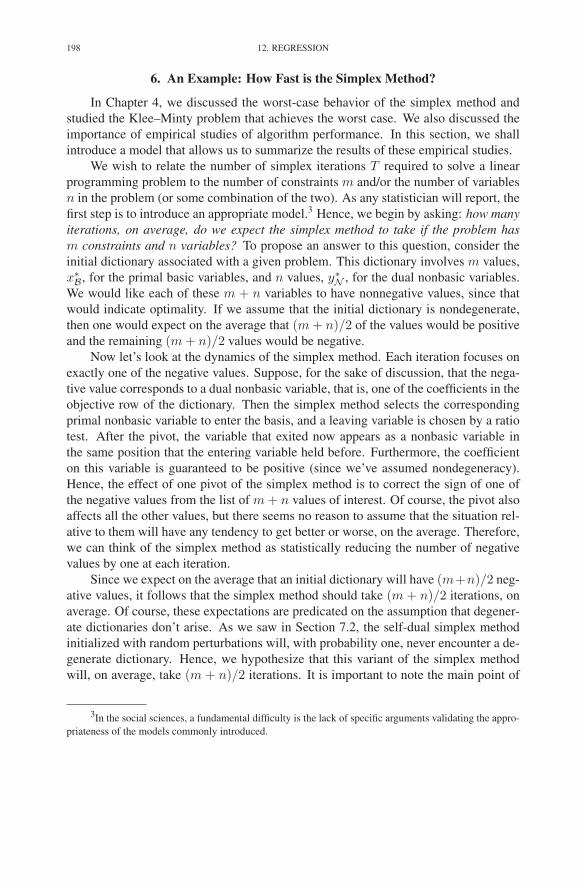
198 12. REGRESSION
6. An Example: How Fast is the Simplex Method?
In Chapter 4, we discussed the worst-case behavior of the simplex method and
studied the Klee–Minty problem that achieves the worst case. We also discussed the
importance of empirical studies of algorithm performance. In this section, we shall
introduce a model that allows us to summarize the results of these empirical studies.
We wish to relate the number of simplex iterations T required to solve a linear
programming problem to the number of constraints m and/or the number of variables
n in the problem (or some combination of the two). As any statistician will report, the
first step is to introduce an appropriate model.3 Hence, we begin by asking: how many
iterations, on average, do we expect the simplex method to take if the problem has
m constraints and n variables? To propose an answer to this question, consider the
initial dictionary associated with a given problem. This dictionary involves m values,
x∗B, for the primal basic variables, and n values, y∗
N , for the dual nonbasic variables.
We would like each of these m + n variables to have nonnegative values, since that
would indicate optimality. If we assume that the initial dictionary is nondegenerate,
then one would expect on the average that (m + n)/2 of the values would be positive
and the remaining (m + n)/2 values would be negative.
Now let’s look at the dynamics of the simplex method. Each iteration focuses on
exactly one of the negative values. Suppose, for the sake of discussion, that the nega-
tive value corresponds to a dual nonbasic variable, that is, one of the coefficients in the
objective row of the dictionary. Then the simplex method selects the corresponding
primal nonbasic variable to enter the basis, and a leaving variable is chosen by a ratio
test. After the pivot, the variable that exited now appears as a nonbasic variable in
the same position that the entering variable held before. Furthermore, the coefficient
on this variable is guaranteed to be positive (since we’ve assumed nondegeneracy).
Hence, the effect of one pivot of the simplex method is to correct the sign of one of
the negative values from the list of m + n values of interest. Of course, the pivot also
affects all the other values, but there seems no reason to assume that the situation rel-
ative to them will have any tendency to get better or worse, on the average. Therefore,
we can think of the simplex method as statistically reducing the number of negative
values by one at each iteration.
Since we expect on the average that an initial dictionary will have (m+n)/2 neg-
ative values, it follows that the simplex method should take (m + n)/2 iterations, on
average. Of course, these expectations are predicated on the assumption that degener-
ate dictionaries don’t arise. As we saw in Section 7.2, the self-dual simplex method
initialized with random perturbations will, with probability one, never encounter a de-
generate dictionary. Hence, we hypothesize that this variant of the simplex method
will, on average, take (m + n)/2 iterations. It is important to note the main point of
3In the social sciences, a fundamental difficulty is the lack of specific arguments validating the appro-
priateness of the models commonly introduced.
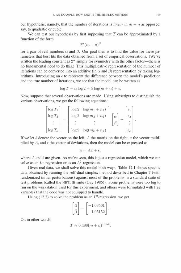
6. AN EXAMPLE: HOW FAST IS THE SIMPLEX METHOD? 199
our hypothesis; namely, that the number of iterations is linear in m + n as opposed,
say, to quadratic or cubic.
We can test our hypothesis by first supposing that T can be approximated by a
function of the form
2α(m + n)β
for a pair of real numbers α and β. Our goal then is to find the value for these pa-
rameters that best fits the data obtained from a set of empirical observations. (We’ve
written the leading constant as 2α simply for symmetry with the other factor—there is
no fundamental need to do this.) This multiplicative representation of the number of
iterations can be converted into an additive (in α and β) representation by taking log-
arithms. Introducing an ǫ to represent the difference between the model’s prediction
and the true number of iterations, we see that the model can be written as
log T = α log 2 + β log(m + n) + ǫ.
Now, suppose that several observations are made. Using subscripts to distinguish the
various observations, we get the following equations:⎡
⎢
⎢
⎢
⎢
⎢
⎣
log T1
log T2
...
log Tk
⎤
⎥
⎥
⎥
⎥
⎥
⎦
=
⎡
⎢
⎢
⎢
⎢
⎢
⎣
log 2 log(m1 + n1)
log 2 log(m2 + n2)...
...
log 2 log(mk + nk)
⎤
⎥
⎥
⎥
⎥
⎥
⎦
[
α
β
]
+
⎡
⎢
⎢
⎢
⎢
⎢
⎣
ǫ1
ǫ2...
ǫk
⎤
⎥
⎥
⎥
⎥
⎥
⎦
.
If we let b denote the vector on the left, A the matrix on the right, x the vector multi-
plied by A, and ǫ the vector of deviations, then the model can be expressed as
b = Ax + ǫ,
where A and b are given. As we’ve seen, this is just a regression model, which we can
solve as an L1-regression or as an L2-regression.
Given real data, we shall solve this model both ways. Table 12.1 shows specific
data obtained by running the self-dual simplex method described in Chapter 7 (with
randomized initial perturbations) against most of the problems in a standard suite of
test problems (called the NETLIB suite (Gay 1985)). Some problems were too big to
run on the workstation used for this experiment, and others were formulated with free
variables that the code was not equipped to handle.
Using (12.2) to solve the problem as an L2-regression, we get[
α
β
]
=
[
−1.03561
1.05152
]
.
Or, in other words,
T ≈ 0.488(m + n)1.052.

200 12. REGRESSION
Name m n iters Name m n iters
25fv47 777 1545 5089 nesm 646 2740 5829
80bau3b 2021 9195 10514 recipe 74 136 80
adlittle 53 96 141 sc105 104 103 92
afiro 25 32 16 sc205 203 202 191
agg2 481 301 204 sc50a 49 48 46
agg3 481 301 193 sc50b 48 48 53
bandm 224 379 1139 scagr25 347 499 1336
beaconfd 111 172 113 scagr7 95 139 339
blend 72 83 117 scfxm1 282 439 531
bnl1 564 1113 2580 scfxm2 564 878 1197
bnl2 1874 3134 6381 scfxm3 846 1317 1886
boeing1 298 373 619 scorpion 292 331 411
boeing2 125 143 168 scrs8 447 1131 783
bore3d 138 188 227 scsd1 77 760 172
brandy 123 205 585 scsd6 147 1350 494
czprob 689 2770 2635 scsd8 397 2750 1548
d6cube 403 6183 5883 sctap1 284 480 643
degen2 444 534 1421 sctap2 1033 1880 1037
degen3 1503 1818 6398 sctap3 1408 2480 1339
e226 162 260 598 seba 449 896 766
etamacro 334 542 1580 share1b 107 217 404
fffff800 476 817 1029 share2b 93 79 189
finnis 398 541 680 shell 487 1476 1155
fit1d 24 1026 925 ship04l 317 1915 597
fit1p 627 1677 15284 ship04s 241 1291 560
forplan 133 415 576 ship08l 520 3149 1091
ganges 1121 1493 2716 ship08s 326 1632 897
greenbea 1948 4131 21476 ship12l 687 4224 1654
grow15 300 645 681 ship12s 417 1996 1360
grow22 440 946 999 sierra 1212 2016 793
grow7 140 301 322 standata 301 1038 74
israel 163 142 209 standmps 409 1038 295
kb2 43 41 63 stocfor1 98 100 81
lotfi 134 300 242 stocfor2 2129 2015 2127
maros 680 1062 2998
TABLE 12.1. Number of iterations for the self-dual simplex method.
This is amazingly close to our hypothesized formula, (m + n)/2. Figure 12.3 shows
a log–log plot of T vs. m + n with the L2-regression line drawn through it. It is clear
from this graph that a straight line (in the log–log plot) is a good model for fitting this
data.
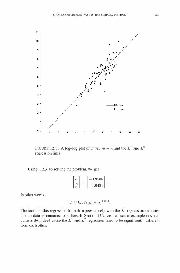
6. AN EXAMPLE: HOW FAST IS THE SIMPLEX METHOD? 201
FIGURE 12.3. A log–log plot of T vs. m + n and the L1 and L2
regression lines.
Using (12.3) to solving the problem, we get
[
α
β
]
=
[
−0.9508
1.0491
]
.
In other words,
T ≈ 0.517(m + n)1.049.
The fact that this regression formula agrees closely with the L2-regression indicates
that the data set contains no outliers. In Section 12.7, we shall see an example in which
outliers do indeed cause the L1 and L2 regression lines to be significantly different
from each other.

202 12. REGRESSION
7. Which Variant of the Simplex Method is Best?
As we saw in the previous section, if the simplex method does not encounter
degenerate dictionaries along its path to optimality, then we can expect that on the
average it will converge in (m + n)/2 iterations. Also, we’ve verified this hypothesis
running the self-dual simplex method (with randomized initial perturbations) against
actual data. The other variants of the simplex method that we have studied do en-
counter degenerate dictionaries and hence we expect them to take more iterations.
To test this hypothesis, we looked at the two-phase simplex method using a dual
Phase I followed by a primal Phase II. The temporary objective function chosen for
Phase I was generated randomly, and hence the Phase I portion of the algorithm en-
countered no degeneracy. However, the Phase II dictionaries were often degenerate
using this method. Figure 12.4 shows a log–log plot of iterations vs. m + n.
The particular code that was used to produce these numbers has not been carefully
tuned, and hence, due to minor numerical problems, the code failed to find an optimal
solution for several of the test problems (even though all the problems in the test suite
are known to have optimal solutions). For these bad problems, one would expect that
the number of iterations to solve the problem is in fact larger (perhaps significantly)
than the number obtained. Nonetheless, Figure 12.4 shows all the results, even those
corresponding to bad problems. The bad data points are shown with open circles.
The figure shows two regression lines. The lower one is the L2-regression line.
Note that it is pulled down significantly by the single outlier at the bottom of the graph.
The upper line is the L1 regression line. Visually it appears to capture better the trend
exhibited by most points. The equation for the L1-regression is
T ≈ 0.877(m + n)0.994.
Again, the hypothesis that the number of iterations is linear in m + n is strongly
supported. But this time the coefficient is obviously not close to 1/2. Instead, it
is almost twice as large. Hence, this method seems to be worse than the self-dual
simplex method.
To reiterate, our conclusion is that degeneracy is bad for iteration counts and any
version of the simplex method that can avoid it will likely do well. To see this effect
in a dramatic setting, let us consider one instance of a large problem that is known to
be highly degenerate. The problem we shall consider is called an assignment problem.
This class of linear programming problem is discussed in detail in Chapter 15. For
now, it suffices to say simply that problems in this class are always degenerate. We
generated one large (m = 600, n = 90,000) random assignment problem and let
the two codes described above solve it. The two-phase code4 took 9951 iterations,
whereas the self-dual code took only 1655—a substantial improvement.
4Unlike the earlier experiments, here the Phase I objective was initialized, without the benefit of
randomization, by setting the jth coefficient to max(cj , 1) where cj is the Phase II objective coefficient.
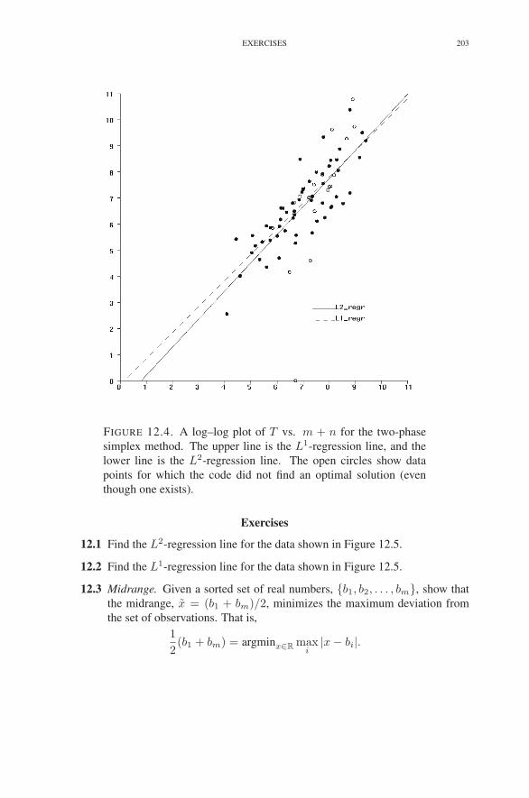
EXERCISES 203
FIGURE 12.4. A log–log plot of T vs. m + n for the two-phase
simplex method. The upper line is the L1-regression line, and the
lower line is the L2-regression line. The open circles show data
points for which the code did not find an optimal solution (even
though one exists).
Exercises
12.1 Find the L2-regression line for the data shown in Figure 12.5.
12.2 Find the L1-regression line for the data shown in Figure 12.5.
12.3 Midrange. Given a sorted set of real numbers, {b1, b2, . . . , bm}, show that
the midrange, x = (b1 + bm)/2, minimizes the maximum deviation from
the set of observations. That is,
1
2(b1 + bm) = argminx∈R
maxi
|x − bi|.
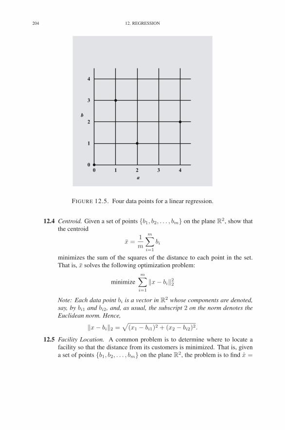
204 12. REGRESSION
a
b
0 1 2 3 40
1
2
3
4
FIGURE 12.5. Four data points for a linear regression.
12.4 Centroid. Given a set of points {b1, b2, . . . , bm} on the plane R2, show that
the centroid
x =1
m
m∑
i=1
bi
minimizes the sum of the squares of the distance to each point in the set.
That is, x solves the following optimization problem:
minimize
m∑
i=1
‖x − bi‖22
Note: Each data point bi is a vector in R2 whose components are denoted,
say, by bi1 and bi2, and, as usual, the subscript 2 on the norm denotes the
Euclidean norm. Hence,
‖x − bi‖2 =√
(x1 − bi1)2 + (x2 − bi2)2.
12.5 Facility Location. A common problem is to determine where to locate a
facility so that the distance from its customers is minimized. That is, given
a set of points {b1, b2, . . . , bm} on the plane R2, the problem is to find x =
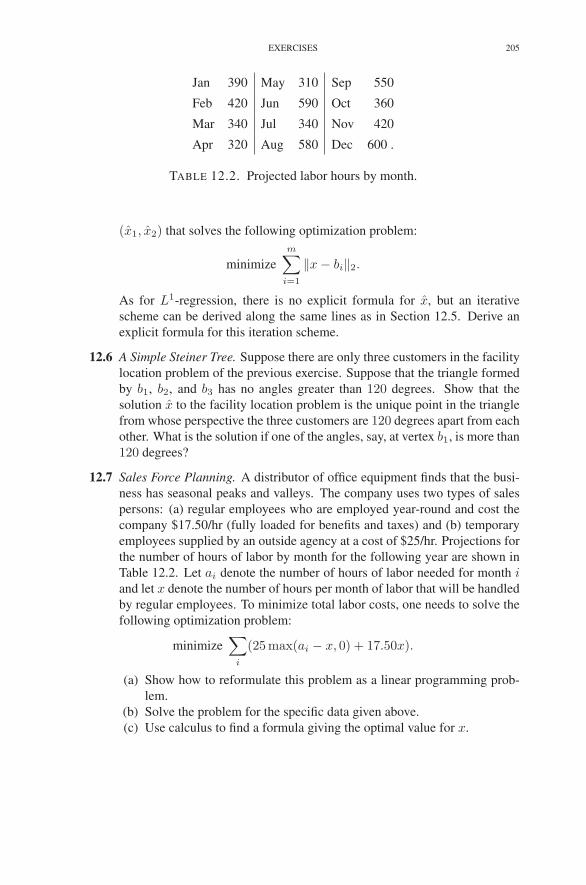
EXERCISES 205
Jan 390 May 310 Sep 550
Feb 420 Jun 590 Oct 360
Mar 340 Jul 340 Nov 420
Apr 320 Aug 580 Dec 600 .
TABLE 12.2. Projected labor hours by month.
(x1, x2) that solves the following optimization problem:
minimize
m∑
i=1
‖x − bi‖2.
As for L1-regression, there is no explicit formula for x, but an iterative
scheme can be derived along the same lines as in Section 12.5. Derive an
explicit formula for this iteration scheme.
12.6 A Simple Steiner Tree. Suppose there are only three customers in the facility
location problem of the previous exercise. Suppose that the triangle formed
by b1, b2, and b3 has no angles greater than 120 degrees. Show that the
solution x to the facility location problem is the unique point in the triangle
from whose perspective the three customers are 120 degrees apart from each
other. What is the solution if one of the angles, say, at vertex b1, is more than
120 degrees?
12.7 Sales Force Planning. A distributor of office equipment finds that the busi-
ness has seasonal peaks and valleys. The company uses two types of sales
persons: (a) regular employees who are employed year-round and cost the
company $17.50/hr (fully loaded for benefits and taxes) and (b) temporary
employees supplied by an outside agency at a cost of $25/hr. Projections for
the number of hours of labor by month for the following year are shown in
Table 12.2. Let ai denote the number of hours of labor needed for month iand let x denote the number of hours per month of labor that will be handled
by regular employees. To minimize total labor costs, one needs to solve the
following optimization problem:
minimize∑
i
(25max(ai − x, 0) + 17.50x).
(a) Show how to reformulate this problem as a linear programming prob-
lem.
(b) Solve the problem for the specific data given above.
(c) Use calculus to find a formula giving the optimal value for x.
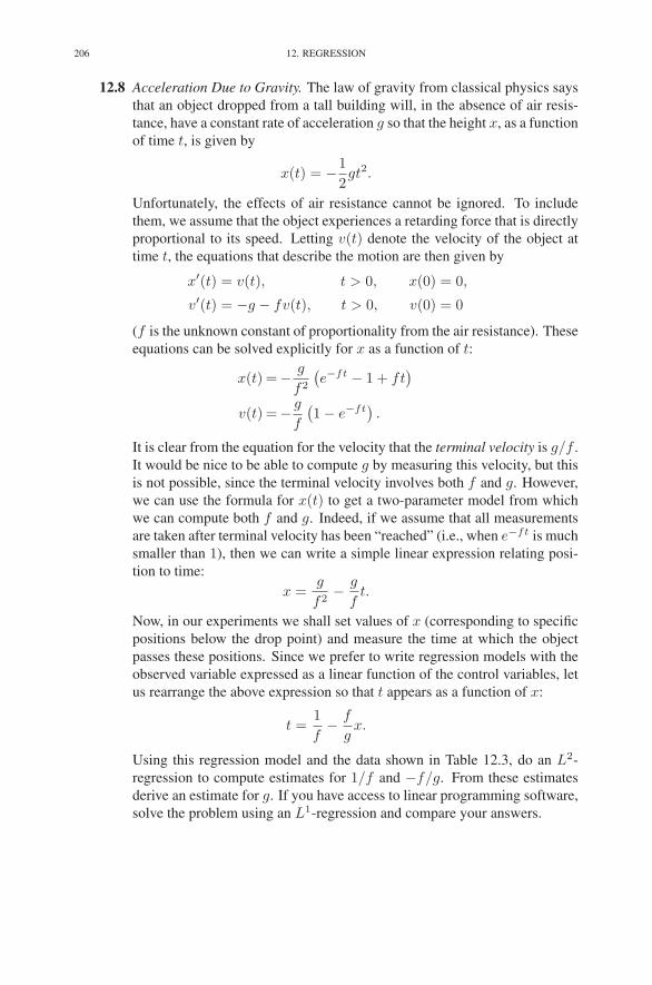
206 12. REGRESSION
12.8 Acceleration Due to Gravity. The law of gravity from classical physics says
that an object dropped from a tall building will, in the absence of air resis-
tance, have a constant rate of acceleration g so that the height x, as a function
of time t, is given by
x(t) = −1
2gt2.
Unfortunately, the effects of air resistance cannot be ignored. To include
them, we assume that the object experiences a retarding force that is directly
proportional to its speed. Letting v(t) denote the velocity of the object at
time t, the equations that describe the motion are then given by
x′(t) = v(t), t > 0, x(0) = 0,
v′(t) = −g − fv(t), t > 0, v(0) = 0
(f is the unknown constant of proportionality from the air resistance). These
equations can be solved explicitly for x as a function of t:
x(t) =− g
f2
(
e−ft − 1 + ft)
v(t) =− g
f
(
1 − e−ft)
.
It is clear from the equation for the velocity that the terminal velocity is g/f .
It would be nice to be able to compute g by measuring this velocity, but this
is not possible, since the terminal velocity involves both f and g. However,
we can use the formula for x(t) to get a two-parameter model from which
we can compute both f and g. Indeed, if we assume that all measurements
are taken after terminal velocity has been “reached” (i.e., when e−ft is much
smaller than 1), then we can write a simple linear expression relating posi-
tion to time:
x =g
f2− g
ft.
Now, in our experiments we shall set values of x (corresponding to specific
positions below the drop point) and measure the time at which the object
passes these positions. Since we prefer to write regression models with the
observed variable expressed as a linear function of the control variables, let
us rearrange the above expression so that t appears as a function of x:
t =1
f− f
gx.
Using this regression model and the data shown in Table 12.3, do an L2-
regression to compute estimates for 1/f and −f/g. From these estimates
derive an estimate for g. If you have access to linear programming software,
solve the problem using an L1-regression and compare your answers.
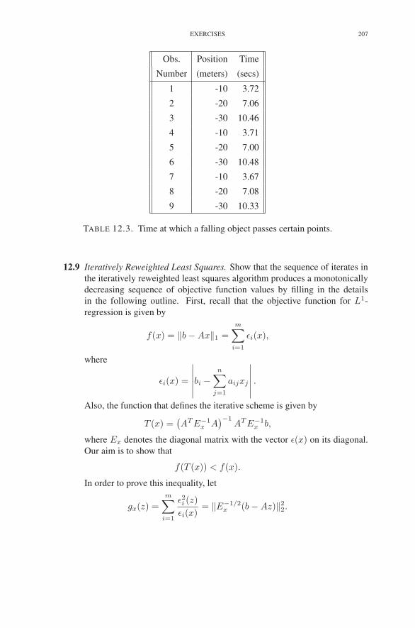
EXERCISES 207
Obs. Position Time
Number (meters) (secs)
1 -10 3.72
2 -20 7.06
3 -30 10.46
4 -10 3.71
5 -20 7.00
6 -30 10.48
7 -10 3.67
8 -20 7.08
9 -30 10.33
TABLE 12.3. Time at which a falling object passes certain points.
12.9 Iteratively Reweighted Least Squares. Show that the sequence of iterates in
the iteratively reweighted least squares algorithm produces a monotonically
decreasing sequence of objective function values by filling in the details
in the following outline. First, recall that the objective function for L1-
regression is given by
f(x) = ‖b − Ax‖1 =
m∑
i=1
ǫi(x),
where
ǫi(x) =
∣
∣
∣
∣
∣
∣
bi −n
∑
j=1
aijxj
∣
∣
∣
∣
∣
∣
.
Also, the function that defines the iterative scheme is given by
T (x) =(
AT E−1x A
)−1AT E−1
x b,
where Ex denotes the diagonal matrix with the vector ǫ(x) on its diagonal.
Our aim is to show that
f(T (x)) < f(x).
In order to prove this inequality, let
gx(z) =m∑
i=1
ǫ2i (z)
ǫi(x)= ‖E−1/2
x (b − Az)‖22.

208 12. REGRESSION
(a) Use calculus to show that, for each x, T (x) is a global minimum of gx.
(b) Show that gx(x) = f(x).(c) By writing
ǫi(T (x)) = ǫi(x) + (ǫi(T (x)) − ǫi(x))
and then substituting the right-hand expression into the definition of
gx(T (x)), show that
gx(T (x)) ≥ 2f(T (x)) − f(x).
(d) Combine the three steps above to finish the proof.
12.10 In our study of means and medians, we showed that the median of a collec-
tion of numbers, b1, b2, . . . , bn, is the number x that minimizes∑
j |x− bj |.Let μ be a real parameter.
(a) Give a statistical interpretation to the following optimization problem:
minimize∑
j
(|x − bj | + μ(x − bj)) .
Hint: the special cases μ = 0,±1/2,±1 might help clarify the general
situation.
(b) Express the above problem as a linear programming problem.
(c) The parametric simplex method can be used to solve families of linear
programming problems indexed by a parameter μ (such as we have
here). Starting at μ = ∞ and proceeding to μ = −∞ one solves
all of the linear programs with just a finite number of pivots. Use the
parametric simplex method to solve the problems of the previous part
in the case where n = 4 and b1 = 1, b2 = 2, b3 = 4, and b4 = 8.
(d) Now consider the general case. Write down the dictionary that appears
in the k-th iteration and show by induction that it is correct.
12.11 Show that the L∞-norm is just the maximum of the absolute values. That
is,
limp→∞
‖x‖p = maxi
|xi|.
Notes
Gonin & Money (1989) and Dodge (1987) are two references on regression that
include discussion of both L2 and L1 regression. The standard reference on L1 re-
gression is Bloomfield & Steiger (1983).
Several researchers, including Smale (1983), Borgwardt (1982), Borgwardt (1987a),
Adler & Megiddo (1985), and Todd (1986), have studied the average number of

NOTES 209
iterations of the simplex method as a function of m and/or n. The model discussed
in this chapter is similar to the sign-invariant model introduced by Adler & Berenguer
(1981).


CHAPTER 13
Financial Applications
In this chapter, we shall study some applications of linear programming to prob-
lems in quantitative finance.
1. Portfolio Selection
Every investor, from the individual to the professional fund manager, must decide
on an appropriate mix of assets to include in his or her investment portfolio. Given a
collection of potential investments (indexed, say, from 1 to n), let Rj denote the return
in the next time period on investment j, j = 1, . . . , n. In general, Rj is a random
variable, although some investments may be essentially deterministic.
A portfolio is determined by specifying what fraction of one’s assets to put into
each investment. That is, a portfolio is a collection of nonnegative numbers xj , j =1, . . . , n, that sum to one. The return (on each dollar) one would obtain using a given
portfolio is given by
R =∑
j
xjRj .
The reward associated with such a portfolio is defined as the expected return1:
ER =∑
j
xjERj .
If reward were the only issue, then the problem would be trivial: simply put everything
in the investment with the highest expected return. But unfortunately, investments
with high reward typically also carry a high level of risk. That is, even though they are
expected to do very well in the long run, they also tend to be erratic in the short term.
There are many ways to define risk, some better than others. We will define the risk
1 In this chapter, we assume a modest familiarity with the ideas and notations of probability:
the symbol E denotes expected value, which means that, if R is a random variable that takes values
R(1), R(2), . . . , R(T ) with equal probability, then
ER =1
T
T∑
t=1
R(t).
211
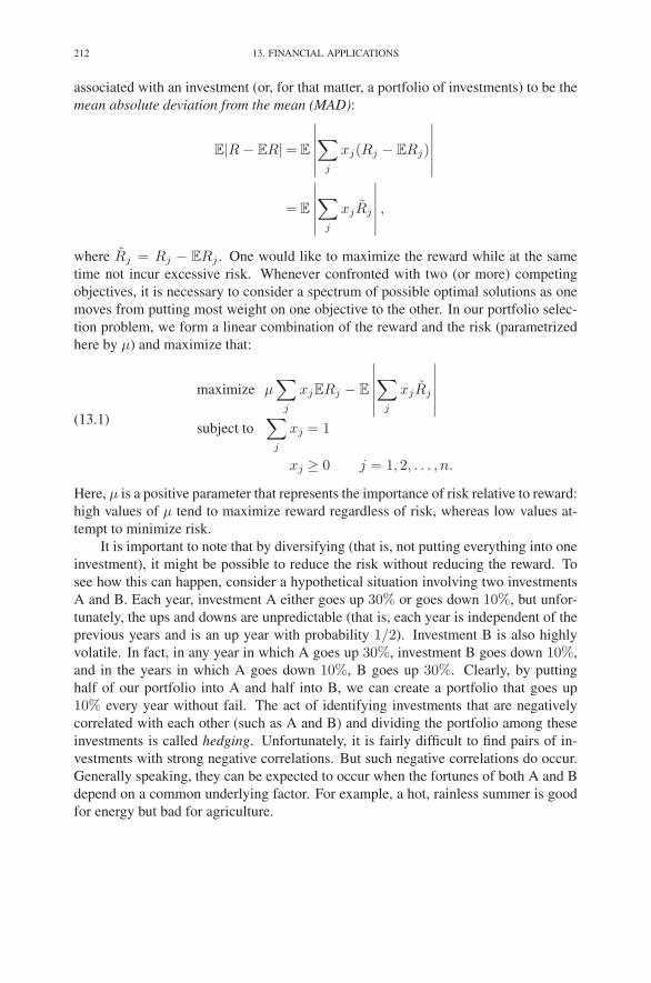
212 13. FINANCIAL APPLICATIONS
associated with an investment (or, for that matter, a portfolio of investments) to be the
mean absolute deviation from the mean (MAD):
E|R − ER|= E
∣
∣
∣
∣
∣
∣
∑
j
xj(Rj − ERj)
∣
∣
∣
∣
∣
∣
= E
∣
∣
∣
∣
∣
∣
∑
j
xjRj
∣
∣
∣
∣
∣
∣
,
where Rj = Rj − ERj . One would like to maximize the reward while at the same
time not incur excessive risk. Whenever confronted with two (or more) competing
objectives, it is necessary to consider a spectrum of possible optimal solutions as one
moves from putting most weight on one objective to the other. In our portfolio selec-
tion problem, we form a linear combination of the reward and the risk (parametrized
here by μ) and maximize that:
(13.1)
maximize μ∑
j
xjERj − E
∣
∣
∣
∣
∣
∣
∑
j
xjRj
∣
∣
∣
∣
∣
∣
subject to∑
j
xj = 1
xj ≥ 0 j = 1, 2, . . . , n.
Here, μ is a positive parameter that represents the importance of risk relative to reward:
high values of μ tend to maximize reward regardless of risk, whereas low values at-
tempt to minimize risk.
It is important to note that by diversifying (that is, not putting everything into one
investment), it might be possible to reduce the risk without reducing the reward. To
see how this can happen, consider a hypothetical situation involving two investments
A and B. Each year, investment A either goes up 30% or goes down 10%, but unfor-
tunately, the ups and downs are unpredictable (that is, each year is independent of the
previous years and is an up year with probability 1/2). Investment B is also highly
volatile. In fact, in any year in which A goes up 30%, investment B goes down 10%,
and in the years in which A goes down 10%, B goes up 30%. Clearly, by putting
half of our portfolio into A and half into B, we can create a portfolio that goes up
10% every year without fail. The act of identifying investments that are negatively
correlated with each other (such as A and B) and dividing the portfolio among these
investments is called hedging. Unfortunately, it is fairly difficult to find pairs of in-
vestments with strong negative correlations. But such negative correlations do occur.
Generally speaking, they can be expected to occur when the fortunes of both A and B
depend on a common underlying factor. For example, a hot, rainless summer is good
for energy but bad for agriculture.

1. PORTFOLIO SELECTION 213
Year- SHY XLB XLE XLF XLI XLK XLP XLU XLV
Month Bonds Materials Energy Financial Indust. Tech. Staples Util. Health
2007-04 1.000 1.044 1.068 1.016 1.035 1.032 1.004 0.987 1.014
2007-03 1.003 1.015 1.051 1.039 1.046 1.047 1.028 1.049 1.073
2007-02 1.005 1.024 1.062 0.994 1.008 1.010 1.021 1.036 1.002
2007-01 1.007 1.027 0.980 0.971 0.989 0.973 0.985 1.053 0.977
2006-12 1.002 1.040 0.991 1.009 1.021 1.020 1.020 0.996 1.030
2006-11 1.001 0.995 0.969 1.030 0.997 0.989 1.020 0.999 1.007
2006-10 1.005 1.044 1.086 1.007 1.024 1.028 0.991 1.026 0.999
2006-09 1.004 1.060 1.043 1.023 1.028 1.040 1.018 1.053 1.003
2006-08 1.004 1.000 0.963 1.040 1.038 1.040 0.999 0.985 1.015
2006-07 1.008 1.030 0.949 1.012 1.011 1.070 1.039 1.028 1.029
2006-06 1.007 0.963 1.034 1.023 0.943 0.974 1.016 1.048 1.055
2006-05 1.002 1.005 1.022 0.995 0.999 0.995 1.018 1.023 1.000
2006-04 1.002 0.960 0.972 0.962 0.983 0.935 1.002 1.016 0.979
2006-03 1.002 1.035 1.050 1.043 1.021 0.987 1.010 1.016 0.969
2006-02 1.002 1.047 1.042 1.003 1.044 1.023 1.008 0.954 0.987
2006-01 1.000 0.978 0.908 1.021 1.031 1.002 1.008 1.013 1.012
2005-12 1.002 1.048 1.146 1.009 1.003 1.034 1.002 1.024 1.013
2005-11 1.004 1.029 1.018 1.000 1.005 0.969 1.001 1.009 1.035
2005-10 1.004 1.076 1.015 1.048 1.058 1.063 1.009 0.999 1.012
2005-09 0.999 1.002 0.909 1.030 0.986 0.977 0.996 0.936 0.969
2005-08 0.997 1.008 1.063 1.009 1.017 1.002 1.014 1.042 0.995
2005-07 1.007 0.958 1.064 0.983 0.976 0.991 0.983 1.006 0.996
2005-06 0.996 1.056 1.071 1.016 1.038 1.057 1.032 1.023 1.023
2005-05 1.002 0.980 1.070 1.012 0.974 0.987 0.981 1.059 0.994
TABLE 13.1. Monthly returns per dollar for each of nine invest-
ments over two years. That is, $1 invested in the energy sector fund
XLE on April 1, 2007, was worth $1.068 on April 30, 2007.
Solving problem (13.1) requires knowledge of the joint distribution of the Rj’s.
However, this distribution is not known theoretically but instead must be estimated
by looking at historical data. For example, Table 13.1 shows monthly returns over a
recent two-year period for one bond fund (3-year Treasury Bonds) and eight differ-
ent sector index funds: Materials (XLB), Energy (XLE), Financial (XLF), Industrial
(XLI), Technology (XLK), Staples (XLP), Utilities (XLU), and Healthcare (XLV).
Let Rj(t) denote the return on investment j over T monthly time periods as shown in
Table 13.1. One way to estimate the mean ERj is simply to take the average of the
historical returns:
ERj =1
T
T∑
t=1
Rj(t).

214 13. FINANCIAL APPLICATIONS
1.1. Reduction to a Linear Programming Problem. As formulated, the prob-
lem in (13.1) is not a linear programming problem. We use the same trick we used
in the previous chapter to replace each absolute value with a new variable and then
impose inequality constraints that ensure that the new variable will indeed be the ap-
propriate absolute value once an optimal value to the problem has been obtained. But
first, let us rewrite (13.1) with the expected value operation replaced by a simple aver-
aging over the given historical data:
(13.2)
maximize μ∑
j
xjrj −1
T
T∑
t=1
∣
∣
∣
∣
∣
∣
∑
j
xj(Rj(t) − rj)
∣
∣
∣
∣
∣
∣
subject to∑
j
xj = 1
xj ≥ 0 j = 1, 2, . . . , n,
where
rj =1
T
T∑
t=1
Rj(t)
denotes the expected reward for asset j. Now, replace∣
∣
∣
∑
j xj(Rj(t) − rj)∣
∣
∣with a
new variable yt and rewrite the optimization problem as
(13.3)
maximize μ∑
j
xjrj −1
T
T∑
t=1
yt
subject to −yt ≤∑
j
xj(Rj(t) − rj)≤ yt t = 1, 2, . . . , T,
∑
j xj = 1
xj ≥ 0 j = 1, 2, . . . , n
yt ≥ 0 t = 1, 2, . . . , T.
As we’ve seen in other contexts before, at optimality one of the two inequalities in-
volving yt must actually be an equality because if both inequalities were strict then it
would be possible to further increase the objective function by reducing yt.
1.2. Solution via Parametric Simplex Method. The problem formulation given
by (13.3) is a linear program that can be solved for any particular value of μ using the
methods described in previous chapters. However, we can do much better than this.
The problem is a parametric linear programming problem, where the parameter is the
risk aversion parameter μ. If we can give a value of μ for which a basic optimal
solution is obvious, then we can start from this basic solution and use the parametric
simplex method to find the optimal solution associated with each and every value of
μ. It is easy to see that for μ larger than some threshold, the optimal solution is to put
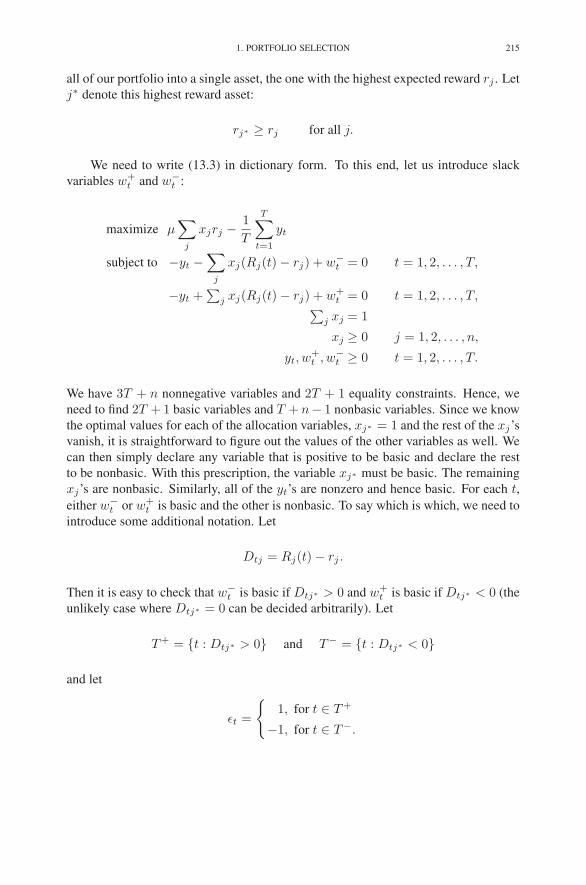
1. PORTFOLIO SELECTION 215
all of our portfolio into a single asset, the one with the highest expected reward rj . Let
j∗ denote this highest reward asset:
rj∗ ≥ rj for all j.
We need to write (13.3) in dictionary form. To this end, let us introduce slack
variables w+t and w−
t :
maximize μ∑
j
xjrj −1
T
T∑
t=1
yt
subject to −yt −∑
j
xj(Rj(t) − rj) + w−t = 0 t = 1, 2, . . . , T,
−yt +∑
j xj(Rj(t) − rj) + w+t = 0 t = 1, 2, . . . , T,
∑
j xj = 1
xj ≥ 0 j = 1, 2, . . . , n,
yt, w+t , w−
t ≥ 0 t = 1, 2, . . . , T.
We have 3T + n nonnegative variables and 2T + 1 equality constraints. Hence, we
need to find 2T + 1 basic variables and T + n− 1 nonbasic variables. Since we know
the optimal values for each of the allocation variables, xj∗ = 1 and the rest of the xj’s
vanish, it is straightforward to figure out the values of the other variables as well. We
can then simply declare any variable that is positive to be basic and declare the rest
to be nonbasic. With this prescription, the variable xj∗ must be basic. The remaining
xj’s are nonbasic. Similarly, all of the yt’s are nonzero and hence basic. For each t,either w−
t or w+t is basic and the other is nonbasic. To say which is which, we need to
introduce some additional notation. Let
Dtj = Rj(t) − rj .
Then it is easy to check that w−t is basic if Dtj∗ > 0 and w+
t is basic if Dtj∗ < 0 (the
unlikely case where Dtj∗ = 0 can be decided arbitrarily). Let
T+ = {t : Dtj∗ > 0} and T− = {t : Dtj∗ < 0}
and let
ǫt =
{
1, for t ∈ T+
−1, for t ∈ T−.

216 13. FINANCIAL APPLICATIONS
It’s tedious, but here’s the optimal dictionary:
ζ = 1T
T∑
t=1
ǫtDtj∗ − 1T
∑
j =j∗
T∑
t=1
ǫt(Dtj − Dtj∗)xj − 1T
∑
t∈T−
w−t − 1
T
∑
t∈T+
w+t
+μrj∗ +μ∑
j =j∗
(rj − rj∗)xj
yt = −Dtj∗ −∑
j =j∗
(Dtj − Dtj∗)xj +w−t t ∈ T−
w−t = 2Dtj∗ +2
∑
j =j∗
(Dtj − Dtj∗)xj +w+t t ∈ T+
yt = Dtj∗ +∑
j =j∗
(Dtj − Dtj∗)xj +w+t t ∈ T+
w+t =−2Dtj∗ −2
∑
j =j∗
(Dtj − Dtj∗)xj +w−t t ∈ T−
xj∗ = 1 −∑
j =j∗
xj
We can now check that, for large μ, this dictionary is optimal. Indeed, the objective
coefficients on the w−t and w+
t variables in the first row of the objective function are
negative. The coefficients on the xj’s in the first row can be positive or negative but for
μ sufficiently large, the negative coefficients on the xj’s in the second row dominate
and make all coefficients negative after considering both rows. Similarly, the fact that
all of the basic variables are positive follows immediately from the definitions of T+
and T−.
A few simple inequalities determine the μ-threshold above which the given dic-
tionary is optimal. The parametric simplex method can then be used to systematically
reduce μ to zero. Along the way, each dictionary encountered corresponds to an op-
timal solution for some range of μ values. Hence, in one pass we have solved the
portfolio selection problem for every investor from the bravest to the most cautious.
Figure 13.1 shows all of the optimal portfolios. The set of all risk–reward profiles that
are possible is shown in Figure 13.2. The lower-right boundary of this set is the so-
called efficient frontier. Any portfolio that produces a risk–reward combination that
does not lie on the efficient frontier can be improved either by increasing its mean
reward without changing the risk or by decreasing the risk without changing the mean
reward. Hence, one should only invest in portfolios that lie on the efficient frontier.
2. Option Pricing
Option pricing is one of the fundamental problems of quantitative finance. In
this section we will describe briefly what an option is and formulate upper and lower
bounds on the price as a linear programming problem.
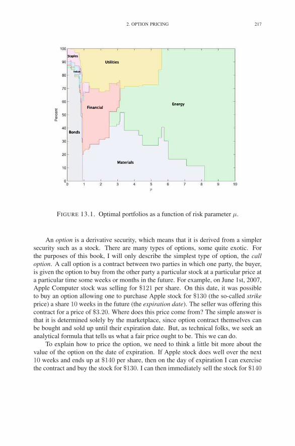
2. OPTION PRICING 217
FIGURE 13.1. Optimal portfolios as a function of risk parameter μ.
An option is a derivative security, which means that it is derived from a simpler
security such as a stock. There are many types of options, some quite exotic. For
the purposes of this book, I will only describe the simplest type of option, the call
option. A call option is a contract between two parties in which one party, the buyer,
is given the option to buy from the other party a particular stock at a particular price at
a particular time some weeks or months in the future. For example, on June 1st, 2007,
Apple Computer stock was selling for $121 per share. On this date, it was possible
to buy an option allowing one to purchase Apple stock for $130 (the so-called strike
price) a share 10 weeks in the future (the expiration date). The seller was offering this
contract for a price of $3.20. Where does this price come from? The simple answer is
that it is determined solely by the marketplace, since option contract themselves can
be bought and sold up until their expiration date. But, as technical folks, we seek an
analytical formula that tells us what a fair price ought to be. This we can do.
To explain how to price the option, we need to think a little bit more about the
value of the option on the date of expiration. If Apple stock does well over the next
10 weeks and ends up at $140 per share, then on the day of expiration I can exercise
the contract and buy the stock for $130. I can then immediately sell the stock for $140
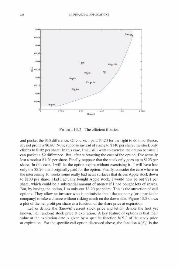
218 13. FINANCIAL APPLICATIONS
FIGURE 13.2. The efficient frontier.
and pocket the $10 difference. Of course, I paid $3.20 for the right to do this. Hence,
my net profit is $6.80. Now, suppose instead of rising to $140 per share, the stock only
climbs to $132 per share. In this case, I will still want to exercise the option because I
can pocket a $2 difference. But, after subtracting the cost of the option, I’ve actually
lost a modest $1.20 per share. Finally, suppose that the stock only goes up to $125 per
share. In this case, I will let the option expire without exercising it. I will have lost
only the $3.20 that I originally paid for the option. Finally, consider the case where in
the intervening 10 weeks some really bad news surfaces that drives Apple stock down
to $100 per share. Had I actually bought Apple stock, I would now be out $21 per
share, which could be a substantial amount of money if I had bought lots of shares.
But, by buying the option, I’m only out $3.20 per share. This is the attraction of call
options. They allow an investor who is optimistic about the economy (or a particular
company) to take a chance without risking much on the down side. Figure 13.3 shows
a plot of the net profit per share as a function of the share price at expiration.
Let s0 denote the (known) current stock price and let S1 denote the (not yet
known, i.e., random) stock price at expiration. A key feature of options is that their
value at the expiration date is given by a specific function h(S1) of the stock price
at expiration. For the specific call option discussed above, the function h(S1) is the

2. OPTION PRICING 219
100 110 120 130 140 150 160-5
0
5
10
15
20
25
30
FIGURE 13.3. A graph of the value of the option at expiration as a
function of stock price. In this example, the strike price is $130.
“hockey-stick” shaped function shown in Figure 13.3. If we think we know the distri-
bution of the random variable S1, then we could compute its expected value and, if we
ignore the discounting for inflation, we could use this to price the option:
p = Eh(S1).
Unfortunately, we generally don’t know the distribution of S1.
We can, however, make some indirect inferences based on “market wisdom” that
constrain the possible values for p and thereby implicitly tell us something about the
distribution of S1. Specifically, let us imagine that there are already a number of
options being traded in the market that are based on the same underlying stock and
have the same expiration date. Let us suppose that there are already n options being
traded in the market with known prices. That is, there are specific functions hj(S1),j = 1, 2, . . . , n, for which there are already known prices pj . One can think of the
underlying stock itself as the simplest possible option. Since the stock is traded, it
too provides some information about the future. We assume that this trivial asset is
the j = 1 option in the collection of known priced options. For this option, we have
h1(S1) = S1 and p1 = s0. To these n options, we add one more: cash. One dollar

220 13. FINANCIAL APPLICATIONS
today will be worth one dollar on the expiration date (again, we are ignoring here the
time value of money). In a sense, this is also and option.
The problem we wish to consider is how to price a new option whose payout
function we denote by g(S1). Consider building a portfolio of the available options
consisting of x0 “shares” of dollars, x1 shares of the underlying stock, and xj shares
of option j (j = 2, . . . , n). Today, this portfolio costs
x0 + x1s0 +
n∑
j=2
xjpj .
At the expiration date, the portolio’s value will be
x0 + x1S1 +
n∑
j=2
xjhj(S1).
Suppose that no matter how S1 turns out, the value of the new option dominates that
of the portfolio:
x0 + x1S1 +n
∑
j=2
xjhj(S1) ≤ g(S1).
Then, it must be the case that the price p of the new option today must also dominate
the cost of this portfolio:
x0 + x1s0 +
n∑
j=2
xjpj ≤ p.
This is called a no-arbitrage condition. This no-arbitrage condition implies a lower
bound p on the price of the new option, which we can maximize:
maximize x0 + x1s0 +
n∑
j=2
xjpj
subject to x0 + x1S1 +n
∑
j=2
xjhj(S1)≤ g(S1).
This problem actually has an infinite number of constraints because the inequality
must hold no matter what value S1 takes on. It can be made into a linear programming
problem by introducing a finite set of possible values, say s1(1), s1(2), . . . , s1(m).The resulting linear programming problem can thus be written as
(13.4)
maximize p = x0 + x1s0 +
n∑
j=2
xjpj
subject to x0 + x1s1(i) +
n∑
j=2
xjhj(s1(i))≤ g(s1(i)), i = 1, . . . , m.

EXERCISES 221
In a completely analogous manner we can find a tight upper bound p for p by solving
a minimization problem:
(13.5)
minimize p = x0 + x1s0 +
n∑
j=2
xjpj
subject to x0 + x1s1(i) +
n∑
j=2
xjhj(s1(i))≥ g(s1(i)), i = 1, . . . , m.
The dual problem associated with (13.4) is
minimize∑
i
g(s1(i))yi
subject to∑
i
yi = 1,
∑
i
s1(i)yi = s0,
∑
i
hj(s1(i))yi = pj , j = 2, . . . , n
yi ≥ 0, i = 1, . . . , m.
Note that the first and last constraints tell us that the yi’s are a system of probabilities.
Given this interpretation of the yi’s as probabilities, the expression
∑
i
s1(i)yi
is just an expected value of the random variable S1 computed using these probabilities.
So, the constraint∑
i s1(i)yi = s0 means that the expected stock price at the end
of the time period must match the current stock price, when computed with the yi
probabilities. For this reason, we call these probabilities risk neutral. Similarly, the
constraints∑
i hj(s1(i))yi = pj , j = 2, . . . , n, tell us that each of the options must
also be priced in such a way that the expected future price matches the current market
price.
Exercises
13.1 Find every portfolio on the efficient frontier using the most recent 6 months
of data for the Bond (SHY), Materials (XLB), Energy (XLE), and Finacial
(XLF) sectors as shown in Table 13.1 (that is, using the upper left 6 × 4subblock of data).

222 13. FINANCIAL APPLICATIONS
13.2 On Planet Claire, markets are highly volatile. Here’s some recent historical
data:
Year- Hair Cosmetics Cash
Month Products
2007-04 1.0 2.0 1.0
2007-03 2.0 2.0 1.0
2007-02 2.0 0.5 1.0
2007-01 0.5 2.0 1.0
Find every portfolio on Planet Claire’s efficient frontier.
13.3 What is the dual of (13.5)?
Notes
The portfolio selection problem originates with Markowitz (1959). He won the
1990 Nobel prize in Economics for this work. In its original formulation, risk is
modeled by the variance of the portfolio’s value rather than the absolute deviation
from the mean considered here. We will discuss the quadratic formulation later in
Chapter 24.
The MAD risk measure we have considered in this chapter has many nice proper-
ties the most important of which is that it produces portfolios that are guaranteed not
to be stochastically dominated (to second order) by other portfolios. Many risk mea-
sures fail to possess this important property. See Ruszczynski & Vanderbei (2003) for
details.
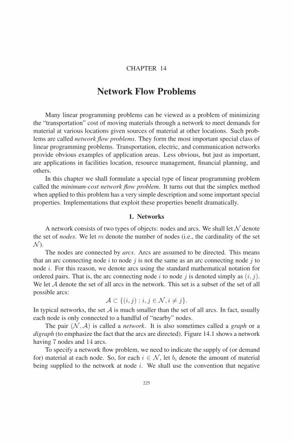
CHAPTER 14
Network Flow Problems
Many linear programming problems can be viewed as a problem of minimizing
the “transportation” cost of moving materials through a network to meet demands for
material at various locations given sources of material at other locations. Such prob-
lems are called network flow problems. They form the most important special class of
linear programming problems. Transportation, electric, and communication networks
provide obvious examples of application areas. Less obvious, but just as important,
are applications in facilities location, resource management, financial planning, and
others.
In this chapter we shall formulate a special type of linear programming problem
called the minimum-cost network flow problem. It turns out that the simplex method
when applied to this problem has a very simple description and some important special
properties. Implementations that exploit these properties benefit dramatically.
1. Networks
A network consists of two types of objects: nodes and arcs. We shall let N denote
the set of nodes. We let m denote the number of nodes (i.e., the cardinality of the set
N ).
The nodes are connected by arcs. Arcs are assumed to be directed. This means
that an arc connecting node i to node j is not the same as an arc connecting node j to
node i. For this reason, we denote arcs using the standard mathematical notation for
ordered pairs. That is, the arc connecting node i to node j is denoted simply as (i, j).We let A denote the set of all arcs in the network. This set is a subset of the set of all
possible arcs:
A ⊂ {(i, j) : i, j ∈ N , i �= j}.In typical networks, the set A is much smaller than the set of all arcs. In fact, usually
each node is only connected to a handful of “nearby” nodes.
The pair (N ,A) is called a network. It is also sometimes called a graph or a
digraph (to emphasize the fact that the arcs are directed). Figure 14.1 shows a network
having 7 nodes and 14 arcs.
To specify a network flow problem, we need to indicate the supply of (or demand
for) material at each node. So, for each i ∈ N , let bi denote the amount of material
being supplied to the network at node i. We shall use the convention that negative
225

226 14. NETWORK FLOW PROBLEMS
a e
d
c b
f g5
−2
−6
−6
9
FIGURE 14.1. A network having 7 nodes and 14 arcs. The numbers
written next to the nodes denote the supply at the node (negative
values indicate demands; missing values indicate no supply or de-
mand).
supplies are in fact demands. Hence, our problem will be to move the material that
sits at the supply nodes over to the demand nodes. The movements must be along the
arcs of the network (and adhering to the directions of the arcs). Since, except for the
supply and demand, there is no other way for material to enter or leave the system,
it follows that the total supply must equal the total demand for the problem to have a
feasible solution. Hence, we shall always assume that
∑
i∈Nbi = 0.
To help us decide the paths along which materials should move, we assume that
each arc, say, (i, j), has associated with it a cost cij that represents the cost of shipping
one unit from i to j directly along arc (i, j). The decision variables then are how
much material to ship along each arc. That is, for each (i, j) ∈ A, xij will denote the
quantity shipped directly from i to j along arc (i, j). The objective is to minimize the
total cost of moving the supply to meet the demand:
minimize∑
(i,j)∈Acijxij .
As we mentioned before, the constraints on the decision variables are that they
ensure flow balance at each node. Let us consider a fixed node, say, k ∈ N . The total
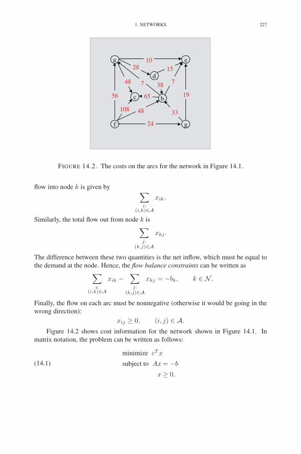
1. NETWORKS 227
a e
d
c b
f g
10
56
108 48
24
33
19
738748
15
65
28
FIGURE 14.2. The costs on the arcs for the network in Figure 14.1.
flow into node k is given by∑
i:(i,k)∈A
xik.
Similarly, the total flow out from node k is∑
j:(k,j)∈A
xkj .
The difference between these two quantities is the net inflow, which must be equal to
the demand at the node. Hence, the flow balance constraints can be written as∑
i:(i,k)∈A
xik −∑
j:(k,j)∈A
xkj = −bk, k ∈ N .
Finally, the flow on each arc must be nonnegative (otherwise it would be going in the
wrong direction):
xij ≥ 0, (i, j) ∈ A.
Figure 14.2 shows cost information for the network shown in Figure 14.1. In
matrix notation, the problem can be written as follows:
(14.1)
minimize cT x
subject to Ax = −b
x≥ 0,

228 14. NETWORK FLOW PROBLEMS
where
xT =[
xac xad xae xba xbc xbe xdb xde xfa xfb xfc xfg xgb xge
]
,
A =
⎡
⎢
⎢
⎢
⎢
⎢
⎢
⎢
⎢
⎢
⎢
⎢
⎢
⎣
−1 −1 −1 1 1
−1 −1 −1 1 1 1
1 1 1
1 −1 −1
1 1 1 1
−1 −1 −1 −1
1 −1 −1
⎤
⎥
⎥
⎥
⎥
⎥
⎥
⎥
⎥
⎥
⎥
⎥
⎥
⎦
, b =
⎡
⎢
⎢
⎢
⎢
⎢
⎢
⎢
⎢
⎢
⎢
⎢
⎢
⎣
0
0
−6
−6
−2
9
5
⎤
⎥
⎥
⎥
⎥
⎥
⎥
⎥
⎥
⎥
⎥
⎥
⎥
⎦
,
cT =[
48 28 10 7 65 7 38 15 56 48 108 24 33 19]
.
In network flow problems, the constraint matrix A is called the node–arc incidence
matrix.
The network flow problem differs from our usual standard form linear program-
ming problem in two respects: (1) it is a minimization instead of a maximization and
(2) the constraints are equalities instead of inequalities. Nonetheless, we have studied
before how duality applies to problems in nonstandard form. The dual of (14.1) is
maximize −bT y
subject to AT y + z = c
z ≥ 0.
Written in network notation, the dual is
maximize −∑
i∈Nbiyi
subject to yj − yi + zij = cij , (i, j) ∈ Azij ≥ 0, (i, j) ∈ A.
Finally, it is not hard to check that the complementarity conditions (to be satisfied by
an optimal primal–dual solution pair) are
xijzij = 0, (i, j) ∈ A.
We shall often refer to the primal variables as primal flows.
2. Spanning Trees and Bases
Network flow problems can be solved efficiently because the basis matrices have
a special structure that can be described nicely in terms of the network. In order to
explain this structure, we need to introduce a number of definitions.
First of all, an ordered list of nodes (n1, n2, . . . , nk) is called a path in the network
if each adjacent pair of nodes in the list is connected by an arc in the network. It is

2. SPANNING TREES AND BASES 229
FIGURE 14.3. The network on the left is connected whereas the
one on the right is not.
FIGURE 14.4. The network on the left contains a cycle whereas the
one on the right is acyclic.
important to note that we do not assume that the arcs point in any particular direction.
For example, for nodes ni and ni+1, there must be an arc in the network. It could
run either from ni to ni+1 or from ni+1 to ni. (One should think about one-way
roads—even though cars can only go one way, pedestrians are allowed to walk along
the path of the road in either direction.) A network is called connected if there is a path
connecting every pair of nodes (see Figure 14.3). For the remainder of this chapter,
we make the following assumption:
Assumption. The network is connected.
For any arc (i, j), we refer to i as its tail and j as its head.
A cycle is a path in which the last node coincides with the first node. A network
is called acyclic if it does not contain any cycles (see Figure 14.4).
A network is a tree if it is connected and acyclic (see Figure 14.5). A network
(N , A) is called a subnetwork of (N ,A) if N ⊂ N and A ⊂ A. A subnetwork
(N , A) is a spanning tree if it is a tree and N = N . Since a spanning tree’s node set
coincides with the node set of the underlying network, it suffices to refer to a spanning
tree by simply giving its arc set.
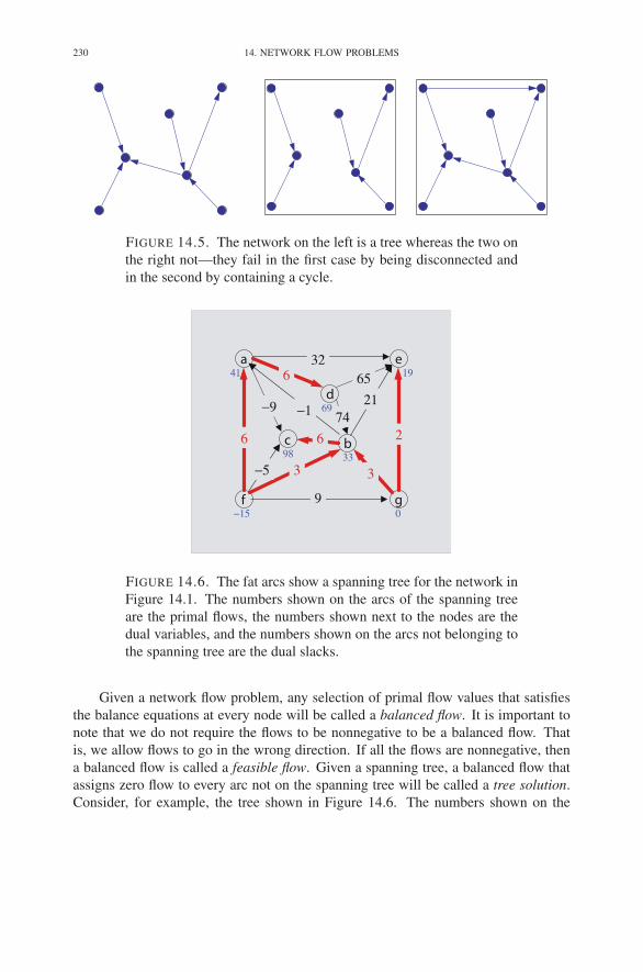
230 14. NETWORK FLOW PROBLEMS
FIGURE 14.5. The network on the left is a tree whereas the two on
the right not—they fail in the first case by being disconnected and
in the second by containing a cycle.
a e
d
c b
f g
32
6
−5 3
9
3
2
2174−1−9
65
6
641
−15
98
19
0
33
69
FIGURE 14.6. The fat arcs show a spanning tree for the network in
Figure 14.1. The numbers shown on the arcs of the spanning tree
are the primal flows, the numbers shown next to the nodes are the
dual variables, and the numbers shown on the arcs not belonging to
the spanning tree are the dual slacks.
Given a network flow problem, any selection of primal flow values that satisfies
the balance equations at every node will be called a balanced flow. It is important to
note that we do not require the flows to be nonnegative to be a balanced flow. That
is, we allow flows to go in the wrong direction. If all the flows are nonnegative, then
a balanced flow is called a feasible flow. Given a spanning tree, a balanced flow that
assigns zero flow to every arc not on the spanning tree will be called a tree solution.
Consider, for example, the tree shown in Figure 14.6. The numbers shown on the

2. SPANNING TREES AND BASES 231
arcs of the spanning tree give the tree solution corresponding to the supplies/demands
shown in Figure 14.1. They were obtained by starting at the “leaves” of the tree and
working “inward.” For instance, the flows could be solved for successively as follows:
flow bal at d: xad = 6,
flow bal at a: xfa − xad = 0 =⇒ xfa = 6,
flow bal at f: −xfa − xfb = −9 =⇒ xfb = 3,
flow bal at c: xbc = 6,
flow bal at b: xfb + xgb − xbc = 0 =⇒ xgb = 3,
flow bal at e: xge = 2.
It is easy to see that this process always works. The reason is that every tree must have
at least one leaf node, and deleting a leaf node together with the edge leading into it
produces a subtree.
The above computation suggests that spanning trees are related to bases in the
simplex method. Let us pursue this idea. Normally, a basis is an invertible square
submatrix of the constraint matrix. But for incidence matrices, no such submatrix
exists. To see why, note that if we sum together all the rows of A, we get a row vector
of all zeros (since each column of A has exactly one +1 and one −1). Of course,
every square submatrix of A has this same property and so is singular. In fact, we
shall show in a moment that for a connected network, there is exactly one redundant
equation (i.e., the rank of A is exactly m − 1).
Let us select some node, say, the last one, and delete the flow-balance constraint
associated with this node from the constraints defining the problem (since it is redun-
dant anyway). Let’s call this node the root node. Let A denote the incidence matrix
A without the row corresponding to the root node (i.e., the last row), and let b denote
the supply/demand vector with the last entry deleted. The most important property of
network flow problems is summarized in the following theorem:
THEOREM 14.1. A square submatrix of A is a basis if and only if the arcs to
which its columns correspond form a spanning tree.
Rather than presenting a formal proof of this theorem, it is more instructive to
explain the idea using the example we’ve been studying. Therefore, consider the
spanning tree shown in Figure 14.6, and let B denote the square submatrix of A cor-
responding to this tree. The matrix B is invertible if and only if every system of
equations of the form
Bu = β
has a unique solution. This is exactly the type of equation that we already solved to
find the tree solution associated with the spanning tree:
BxB = −b.
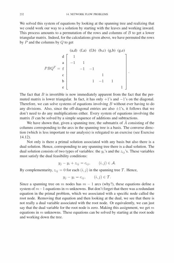
232 14. NETWORK FLOW PROBLEMS
We solved this system of equations by looking at the spanning tree and realizing that
we could work our way to a solution by starting with the leaves and working inward.
This process amounts to a permutation of the rows and columns of B to get a lower
triangular matrix. Indeed, for the calculations given above, we have permuted the rows
by P and the columns by Q to get
PBQT =
(a,d) (f,a) (f,b) (b,c) (g,b) (g,e)
d
a
f
c
b
e
⎡
⎢
⎢
⎢
⎢
⎢
⎢
⎢
⎢
⎢
⎣
1
−1 1
−1 −1
1
1 −1 1
1
⎤
⎥
⎥
⎥
⎥
⎥
⎥
⎥
⎥
⎥
⎦
.
The fact that B is invertible is now immediately apparent from the fact that the per-
muted matrix is lower triangular. In fact, it has only +1’s and −1’s on the diagonal.
Therefore, we can solve systems of equations involving B without ever having to do
any divisions. Also, since the off-diagonal entries are also ±1’s, it follows that we
don’t need to do any multiplications either. Every system of equations involving the
matrix B can be solved by a simple sequence of additions and subtractions.
We have shown that, given a spanning tree, the submatrix of A consisting of the
columns corresponding to the arcs in the spanning tree is a basis. The converse direc-
tion (which is less important to our analysis) is relegated to an exercise (see Exercise
14.12).
Not only is there a primal solution associated with any basis but also there is a
dual solution. Hence, corresponding to any spanning tree there is a dual solution. The
dual solution consists of two types of variables: the yi’s and the zij’s. These variables
must satisfy the dual feasibility conditions:
yj − yi + zij = cij , (i, j) ∈ A.
By complementarity, zij = 0 for each (i, j) in the spanning tree T . Hence,
yj − yi = cij , (i, j) ∈ T .
Since a spanning tree on m nodes has m − 1 arcs (why?), these equations define a
system of m−1 equations in m unknowns. But don’t forget that there was a redundant
equation in the primal problem, which we associated with a specific node called the
root node. Removing that equation and then looking at the dual, we see that there is
not really a dual variable associated with the root node. Or equivalently, we can just
say that the dual variable for the root node is zero. Making this assignment, we get mequations in m unknowns. These equations can be solved by starting at the root node
and working down the tree.

3. THE PRIMAL NETWORK SIMPLEX METHOD 233
For example, let node “g” be the root node in the spanning tree in Figure 14.6.
Starting with it, we compute the dual variables as follows:
yg = 0,
across arc (g,e): ye − yg = 19 =⇒ ye = 19,
across arc (g,b): yb − yg = 33 =⇒ yb = 33,
across arc (b,c): yc − yb = 65 =⇒ yc = 98,
across arc (f,b): yb − yf = 48 =⇒ yf = −15,
across arc (f,a): ya − yf = 56 =⇒ ya = 41,
across arc (a,d): yd − ya = 28 =⇒ yd = 69.
Now that we know the dual variables, the dual slacks for the arcs not in the spanning
tree T can be computed using
zij = yi + cij − yj , (i, j) �∈ T(which is just the dual feasibility condition solved for zij). These values are shown on
the nontree arcs in Figure 14.6.
From duality theory, we know that the current tree solution is optimal if all the
flows are nonnegative and if all the dual slacks are nonnegative. The tree solution
shown in Figure 14.6 satisfies the first condition but not the second. That is, it is
primal feasible but not dual feasible. Hence, we can apply the primal simplex method
to move from this solution to an optimal one. We take up this task in the next section.
3. The Primal Network Simplex Method
Each of the variants of the simplex method presented in earlier chapters of this
book can be applied to network flow problems. It would be overkill to describe them
all here in the context of networks. However, they are all built on two simple algo-
rithms: the primal simplex method (for problems that are primal feasible) and the dual
simplex method (for problems that are dual feasible). We discuss them both in detail.
We shall describe the primal network simplex method by continuing with our
example. As mentioned above, the tree shown in Figure 14.6 is primal feasible but
not dual feasible. The basic idea that defines the primal simplex method is to pick a
nontree arc that is dual infeasible and let it enter the tree (i.e., become basic) and then
readjust everything so that we still have a tree solution.
The First Iteration. For our first pivot, we let arc (a,c) enter the tree using a primal
pivot. In a primal pivot, we add flow to the entering variable, keeping all other nontree
flows set to zero and adjusting the tree flows appropriately to maintain flow balance.
Given any spanning tree, adding an extra arc must create a cycle (why?). Hence, the
current spanning tree together with the entering arc must contain a cycle. The flows
on the cycle must change to accommodate the increasing flow on the entering arc. The
flows on the other tree arcs remain unchanged. In our example, the cycle is: “a”, “c”,
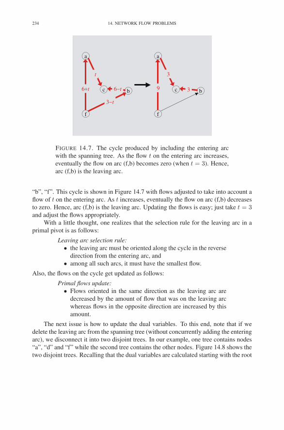
234 14. NETWORK FLOW PROBLEMS
a
c b
f
6+t
3−t
t
6−t
a
c b
f
9
3
3
FIGURE 14.7. The cycle produced by including the entering arc
with the spanning tree. As the flow t on the entering arc increases,
eventually the flow on arc (f,b) becomes zero (when t = 3). Hence,
arc (f,b) is the leaving arc.
“b”, “f”. This cycle is shown in Figure 14.7 with flows adjusted to take into account a
flow of t on the entering arc. As t increases, eventually the flow on arc (f,b) decreases
to zero. Hence, arc (f,b) is the leaving arc. Updating the flows is easy; just take t = 3and adjust the flows appropriately.
With a little thought, one realizes that the selection rule for the leaving arc in a
primal pivot is as follows:
Leaving arc selection rule:
• the leaving arc must be oriented along the cycle in the reverse
direction from the entering arc, and
• among all such arcs, it must have the smallest flow.
Also, the flows on the cycle get updated as follows:
Primal flows update:
• Flows oriented in the same direction as the leaving arc are
decreased by the amount of flow that was on the leaving arc
whereas flows in the opposite direction are increased by this
amount.
The next issue is how to update the dual variables. To this end, note that if we
delete the leaving arc from the spanning tree (without concurrently adding the entering
arc), we disconnect it into two disjoint trees. In our example, one tree contains nodes
“a”, “d” and “f” while the second tree contains the other nodes. Figure 14.8 shows the
two disjoint trees. Recalling that the dual variables are calculated starting with the root

3. THE PRIMAL NETWORK SIMPLEX METHOD 235
a e
d
c b
f g
?
?
? ?
?
3
2
21???
?
?
6?
?
98
19
0
33
?
FIGURE 14.8. The two disjoint trees. Primal and dual values that
remained unchanged are shown, whereas those that need to be up-
dated are shown as question marks.
node and working up the spanning tree, it is clear that the dual variables on the subtree
containing the root node remain unchanged, whereas those on the other subtree must
change. For the current pivot, the other subtree consists of nodes “a”, “d”, and “f”.
They all get incremented by the same fixed amount, since the only change is that the
arc by which we bridged from the root-containing tree to this other tree has changed
from the leaving arc to the entering arc. Looking at node “a” and using tildes to denote
values after being changed, we see that
ya = yc − cac
= yc − cac,
whereas
zac = ya + cac − yc.
Combining these two equations, we get
ya = ya − zac.
That is, the dual variable at node “a” gets decremented by zac = −9. Of course, all
of the dual variables on this subtree get decremented by this same amount. In general,
the dual variable update rule can be stated as follows:
Dual variables update:
• If the entering arc crosses from the root-containing tree to the
non-root-containing tree, then increase all dual variables on

236 14. NETWORK FLOW PROBLEMS
a e
d
c b
f g
41
9
4 9
18
3
2
2183−103
74
3
650
−6
98
19
0
33
78
FIGURE 14.9. The tree solution at the end of the first iteration.
the non-root-containing tree by the dual slack of the entering
arc.
• Otherwise, decrease these dual variables by this amount.
Finally, we must update the dual slacks. The only dual slacks that change are
those that span across the two trees since, for these nodes, either the head or the tail
dual variable changes, while the other does not. Those that span the two subtrees in
the same direction as the entering arc must be decreased by zac, whereas those that
bridge the two trees in the opposite direction must be increased by this amount. For
our example, six nontree arcs, (f,g), (f,b), (f,c), (d,b), (d,e), and (a,e), span in the same
direction as the entering arc. They all must be decreased by −9. That is, they must be
increased by 9. For example, the dual slack on arc (f,c) changes from −5 to 4. Only
one arc, (b,a), spans in the other direction. It must be decreased by 9. The updated
solution is shown in Figure 14.9. The general rule for updating the dual slacks is as
follows:
Dual slacks update:
• The dual slacks corresponding to those arcs that bridge in the
same direction as the entering arc get decremented by the old
dual slack on the entering arc, whereas those that correspond
to arcs bridging in the opposite direction get incremented by
this amount.
The Second Iteration. The tree solution shown in Figure 14.9 has only one re-
maining infeasibility: zba = −10. Arc (b,a) must therefore enter the spanning tree.
Adding it, we create a cycle consisting of nodes “a”, “b”, and “c”. The leaving arc
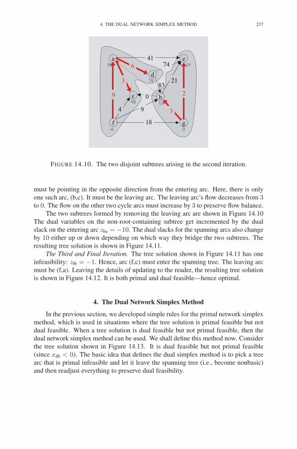
4. THE DUAL NETWORK SIMPLEX METHOD 237
83
a e
d
c b
f g
41
9
4 9
18
3
2
213
74
0
650
−6
98
19
0
33
78
FIGURE 14.10. The two disjoint subtrees arising in the second iteration.
must be pointing in the opposite direction from the entering arc. Here, there is only
one such arc, (b,c). It must be the leaving arc. The leaving arc’s flow decreases from 3to 0. The flow on the other two cycle arcs must increase by 3 to preserve flow balance.
The two subtrees formed by removing the leaving arc are shown in Figure 14.10
The dual variables on the non-root-containing subtree get incremented by the dual
slack on the entering arc zba = −10. The dual slacks for the spanning arcs also change
by 10 either up or down depending on which way they bridge the two subtrees. The
resulting tree solution is shown in Figure 14.11.
The Third and Final Iteration. The tree solution shown in Figure 14.11 has one
infeasibility: zfb = −1. Hence, arc (f,c) must enter the spanning tree. The leaving arc
must be (f,a). Leaving the details of updating to the reader, the resulting tree solution
is shown in Figure 14.12. It is both primal and dual feasible—hence optimal.
4. The Dual Network Simplex Method
In the previous section, we developed simple rules for the primal network simplex
method, which is used in situations where the tree solution is primal feasible but not
dual feasible. When a tree solution is dual feasible but not primal feasible, then the
dual network simplex method can be used. We shall define this method now. Consider
the tree solution shown in Figure 14.13. It is dual feasible but not primal feasible
(since xdb < 0). The basic idea that defines the dual simplex method is to pick a tree
arc that is primal infeasible and let it leave the spanning tree (i.e., become nonbasic)
and then readjust everything to preserve dual feasibility.

238 14. NETWORK FLOW PROBLEMS
a e
d
c b
f g
31
9
4 −1
8
3
2
217336
64
10
640
−16
88
19
0
33
68
FIGURE 14.11. The tree solution at the end of the second iteration.
To get from the spanning tree in Figure 14.9 to here, we let arc (b,a)
enter and arc (b,c) leave.
a e
d
c b
f g
31
1
5 9
9
3
2
2173126
64
10
640
−15
88
19
0
33
68
FIGURE 14.12. The tree solution at the end of the third iteration.
To get from the spanning tree in Figure 14.11 to here, we let arc (f,b)
enter and arc (f,a) leave. This tree solution is the optimal solution to
the problem.
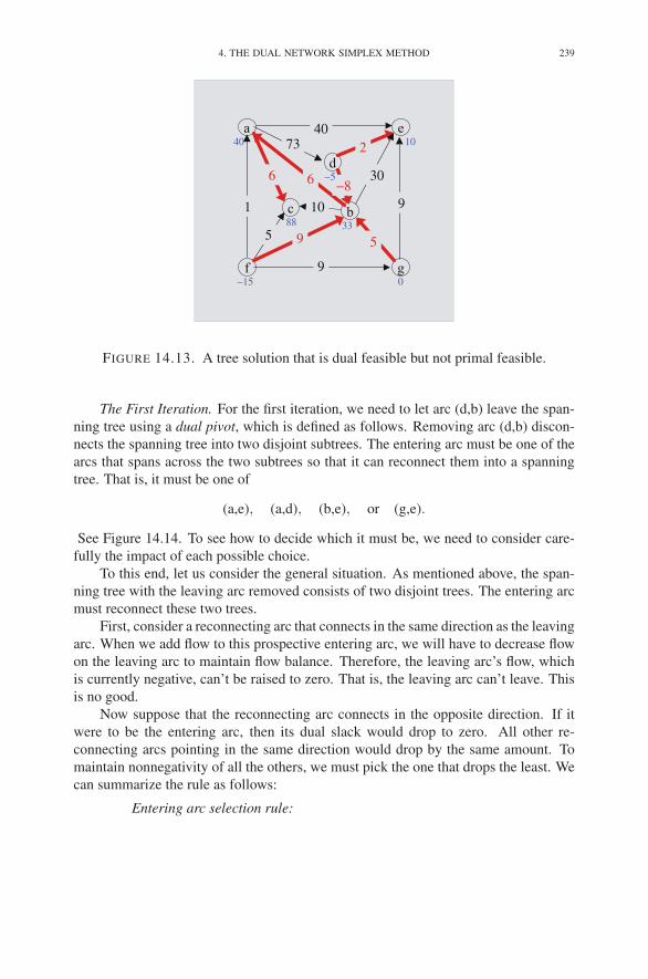
4. THE DUAL NETWORK SIMPLEX METHOD 239
a e
d
c b
f g
40
1
5 9
9
5
9
30−866
2
10
7340
−15
88
10
0
33
−5
FIGURE 14.13. A tree solution that is dual feasible but not primal feasible.
The First Iteration. For the first iteration, we need to let arc (d,b) leave the span-
ning tree using a dual pivot, which is defined as follows. Removing arc (d,b) discon-
nects the spanning tree into two disjoint subtrees. The entering arc must be one of the
arcs that spans across the two subtrees so that it can reconnect them into a spanning
tree. That is, it must be one of
(a,e), (a,d), (b,e), or (g,e).
See Figure 14.14. To see how to decide which it must be, we need to consider care-
fully the impact of each possible choice.
To this end, let us consider the general situation. As mentioned above, the span-
ning tree with the leaving arc removed consists of two disjoint trees. The entering arc
must reconnect these two trees.
First, consider a reconnecting arc that connects in the same direction as the leaving
arc. When we add flow to this prospective entering arc, we will have to decrease flow
on the leaving arc to maintain flow balance. Therefore, the leaving arc’s flow, which
is currently negative, can’t be raised to zero. That is, the leaving arc can’t leave. This
is no good.
Now suppose that the reconnecting arc connects in the opposite direction. If it
were to be the entering arc, then its dual slack would drop to zero. All other re-
connecting arcs pointing in the same direction would drop by the same amount. To
maintain nonnegativity of all the others, we must pick the one that drops the least. We
can summarize the rule as follows:
Entering arc selection rule:

240 14. NETWORK FLOW PROBLEMS
a e
d
c b
f g
40
1
5 9
9
5
9
3066
2
10
7340
−15
88
10
0
33
−5
FIGURE 14.14. The two subtrees for the first pivot of the dual sim-
plex method.
• the entering arc must bridge the two subtrees in the opposite
direction from the leaving arc, and
• among all such arcs, it must have the smallest dual slack.
In our example, all bridging arcs point in the opposite direction from the leaving arc.
The one with the smallest dual slack is (g,e) whose slack is zge = 9. This arc must be
the entering arc.
We have now determined both the entering and leaving arcs. Hence, the new
spanning tree is determined and therefore, in principle, all the variables associated
with this new spanning tree can be computed. Furthermore, the rules for determining
the new values by updating from the previous ones are the same as in the primal
network simplex method. The resulting tree solution is shown in Figure 14.15.
The Second Iteration. For the second pivot, there are two choices for the leaving
arc: (g,b) and (d,e). Using the most infeasible, we choose (d,e). We remove this arc
from the spanning tree to produce two subtrees. One of the subtrees consists of just
the node “d” all by itself while the other subtree consists of the rest of the nodes.
Remembering that the reconnecting arc must bridge the two subtrees in the opposite
direction, the only choice is (a,d). So this arc is the entering arc. Making the pivot, we
arrive at the optimal tree solution shown in Figure 14.12.
5. Putting It All Together
As we saw in Chapter 5, for linear programming the primal and the dual simplex
methods form the foundation on which one can build a few different variants of the
simplex method. The same is true here in the context of network flows.

5. PUTTING IT ALL TOGETHER 241
a e
d
c b
f g
31
1
5 9
9
−3
8
21966
−6
10
6440
−15
88
19
0
33
4
FIGURE 14.15. The tree solution after the first pivot.
For example, one can build a two-phased procedure in which one first uses the
dual network simplex method (with costs artificially and temporarily altered to ensure
dual feasibility of an initial tree solution) to find a primal feasible solution and then
uses the primal network simplex method to move from the feasible solution to an
optimal one.
Alternatively, one can use the primal network simplex method (with supplies tem-
porarily altered to ensure primal feasibility of an initial tree solution) to find a dual
feasible solution and then use the dual network simplex method (with the original
supplies) to move from the dual feasible solution to an optimal one.
Finally, as described for linear programming in Chapter 7, one can define a para-
metric self-dual method in which primal pivots and dual pivots are intermingled as
needed so as to reduce a perturbation parameter μ from ∞ to zero.
Since there is nothing new in how one builds the network versions of these algo-
rithms from the basic primal and dual simplex pivots, we don’t go through any exam-
ples here. Instead, we just mention one final observation about the dual variables, the
yi’s. Namely, they are not needed anywhere in the performance of a primal or a dual
pivot. Hence, their calculation is entirely optional and can be skipped altogether or
simply defered to the end.
For completeness, we end this section by giving a step-by-step description of the
self-dual network simplex method. The steps are as follows:
(1) Identify a spanning tree—any one will do (see Exercise 14.14). Also identify
a root node.
(2) Compute initial primal flows on the tree arcs by assuming that nontree arcs
have zero flow and the total flow at each node must be balanced. For this

242 14. NETWORK FLOW PROBLEMS
calculation, the computed primal flows may be negative. In this case, the
initial primal solution is not feasible. The calculation is performed working
from leaf nodes inward.
(3) Compute initial dual values by working out from the root node along tree
arcs using the formula
yj − yi = cij ,
which is valid on tree arcs, since the dual slacks vanish on these arcs.
(4) Compute initial dual slacks on each nontree arc using the formula
zij = yi + cij − yj .
Again, some of the zij’s might be nonnegative. This is okay (for now), but
it is important that they satisfy the above equality.
(5) Perturb each primal flow and each dual slack that has a negative initial value
by adding a positive scalar μ to each such value.
(6) Identify a range μMIN ≤ μ ≤ μMAX over which the current solution is optimal
(on the first iteration, μMAX will be infinite).
(7) Check the stopping rule: if μMIN ≤ 0, then set μ = 0 to recover an optimal
solution. While not optimal, perform each of the remaining steps and then
return to recheck this condition.
(8) Select an arc associated with the inequality μMIN ≤ μ (if there are several,
pick one arbitrarily). If this arc is a nontree arc, then the current pivot is a
primal pivot. If, on the other hand, it is a tree arc, then the pivot is a dual
pivot.
(a) If the pivot is a primal pivot, the arc identified above is the entering arc.
Identify the associated leaving arc as follows. First, add the entering arc
to the tree. With this arc added, there must be a cycle consisting of the
entering arc and other tree arcs. The leaving arc is chosen from those
arcs on the cycle that go in the opposite direction from the entering arc
and having the smallest flow among all such arcs (evaluated at μ =μMIN).
(b) If the pivot is a dual pivot, the arc identified above is the leaving arc.
Identify the associated entering arc as follows. First, delete the leaving
arc from the tree. This deletion splits the tree into two subtrees. The
entering arc must bridge these two trees in the opposite direction to the
leaving arc, and, among such arcs, it must be the one with the smallest
dual slack (evaluated at μ = μMIN).
(9) Update primal flows as follows. Add the entering arc to the tree. This ad-
dition creates a cycle containing both the entering and leaving arcs. Adjust
the flow on the leaving arc to zero, and then adjust the flows on each of the
other cycle arcs as necessary to maintain flow balance.

6. THE INTEGRALITY THEOREM 243
(10) Update dual variables as follows. Delete the leaving arc from the old tree.
This deletion splits the old tree into two subtrees. Let Tu denote the subtree
containing the tail of the entering arc, and let Tv denote the subtree contain-
ing its head. The dual variables for nodes in Tu remain unchanged, but the
dual variables for nodes in Tv get incremented by the old dual slack on the
entering arc.
(11) Update dual slacks as follows. All dual slacks remain unchanged except for
those associated with nontree arcs that bridge the two subtrees Tu and Tv .
The dual slacks corresponding to those arcs that bridge in the same direction
as the entering arc get decremented by the old dual slack on the entering arc,
whereas those that correspond to arcs bridging in the opposite direction get
incremented by this amount.
As was said before and should now be clear, there is no need to update the dual vari-
ables from one iteration to the next; that is, step 10 can be skipped.
6. The Integrality Theorem
In this section, we consider network flow problems for which all the supplies and
demands are integers. Such problems are called network flow problems with integer
data. As we explained in Section 14.2, for network flow problems, basic primal so-
lutions are computed without any multiplication or division. The following important
theorem follows immediately from this property:
THEOREM 14.2. Integrality Theorem. For network flow problems with integer
data, every basic feasible solution and, in particular, every basic optimal solution
assigns integer flow to every arc.
This theorem is important because many real-world network flow problems have
integral supplies/demands and require their solutions to be integral too. This inte-
grality restriction typically occurs when one is shipping indivisible units through a
network. For example, it wouldn’t make sense to ship one third of a car from an au-
tomobile assembly plant to one dealership with the other two thirds going to another
dealership.
Problems that are linear programming problems with the additional stipulation
that the optimal solution values must be integers are called integer programming prob-
lems. Generally speaking, these problems are much harder to solve than linear pro-
gramming problems (see Chapter 23). However, if the problem is a network flow
problem with integer data, it can be solved efficiently using the simplex method to
compute a basic optimal solution, which the integrality theorem tells us will be integer
valued.
6.1. Konig’s Theorem. In addition to its importance in real-world optimization
problems, the integrality theorem also has many applications to the branch of mathe-
matics called combinatorics. We illustrate with just one example.

244 14. NETWORK FLOW PROBLEMS
THEOREM 14.3. Konig’s Theorem. Suppose that there are n girls and n boys,
that every girl knows exactly k boys, and that every boy knows exactly k girls. Then nmarriages can be arranged with everybody knowing his or her spouse.
Before proving this theorem it is important to clarify its statement by saying that
the property of “knowing” is symmetric (for example, knowing in the biblical sense).
That is, if a certain girl knows a certain boy, then this boy also knows this girl.
PROOF. Consider a network with nodes g1, g2, . . . , gn, b1, b2, . . . , bn and an arc
from gi to bj if girl i and boy j know each other. Assign one unit of supply to each girl
node and a unit of demand to each boy node. Assign arbitrary objective coefficients to
create a well-defined network flow problem. The problem is guaranteed to be feasible:
just put a flow of 1/k on each arc (the polygamists in the group might prefer this
nonintegral solution). By the integrality theorem, the problem has an integer-valued
solution. Clearly, the flow on each arc must be either zero or one. Also, each girl
node is the tail of exactly one arc having a flow of one. This arc points to her intended
mate. �
Exercises
In solving the following problems, the network pivot tool can be used to check
your arithmetic:
campuscgi.princeton.edu/∼rvdb/JAVA/network/nettool/netsimp.html
14.1 Consider the following network flow problem:
f0
e
d
a
c
b
h
g
i11
5
0
6
3
1
−3
12 103
51 5
3
1
7
6
−8
3
8
17
−3
−8
−9 0
Numbers shown above the nodes are supplies (negative values represent de-
mands) and numbers shown above the arcs are unit shipping costs. The
darkened arcs form a spanning tree.
(a) Compute primal flows for each tree arc.
(b) Compute dual variables for each node.
(c) Compute dual slacks for each nontree arc.
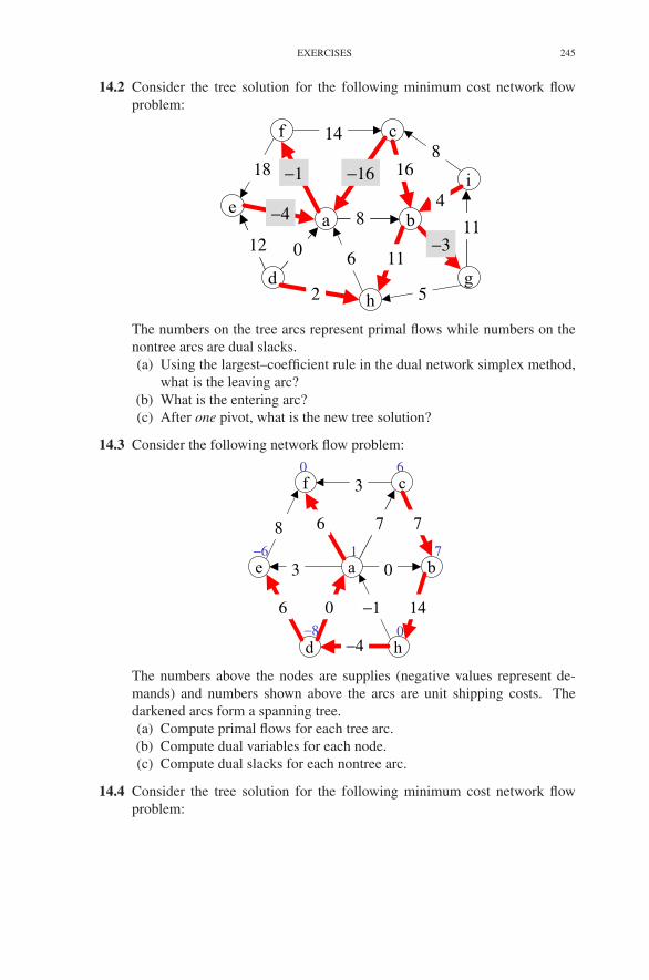
EXERCISES 245
14.2 Consider the tree solution for the following minimum cost network flow
problem:
f
e
d
a
c
b
h
g
i18
14
−1
−4
12
2
8
−16 168
110 11
5
−3
4
6
The numbers on the tree arcs represent primal flows while numbers on the
nontree arcs are dual slacks.
(a) Using the largest–coefficient rule in the dual network simplex method,
what is the leaving arc?
(b) What is the entering arc?
(c) After one pivot, what is the new tree solution?
14.3 Consider the following network flow problem:
f
e
d
a
c
b
h
8
3
6
3
6
−4
0
7 7
0 14−1
−6
−8 0
1 7
0 6
The numbers above the nodes are supplies (negative values represent de-
mands) and numbers shown above the arcs are unit shipping costs. The
darkened arcs form a spanning tree.
(a) Compute primal flows for each tree arc.
(b) Compute dual variables for each node.
(c) Compute dual slacks for each nontree arc.
14.4 Consider the tree solution for the following minimum cost network flow
problem:
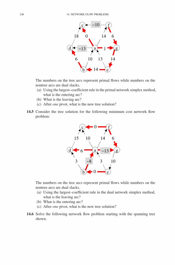
246 14. NETWORK FLOW PROBLEMS
c
d
b
a
f
g
e
18
−10
0
−13
6
14
1
14 6
10 1413
The numbers on the tree arcs represent primal flows while numbers on the
nontree arcs are dual slacks.
(a) Using the largest–coefficient rule in the primal network simplex method,
what is the entering arc?
(b) What is the leaving arc?
(c) After one pivot, what is the new tree solution?
14.5 Consider the tree solution for the following minimum cost network flow
problem:
c
d
b
a
f
g
e
15
0
10
6
3
0
−13
14 6
−8 103
The numbers on the tree arcs represent primal flows while numbers on the
nontree arcs are dual slacks.
(a) Using the largest–coefficient rule in the dual network simplex method,
what is the leaving arc?
(b) What is the entering arc?
(c) After one pivot, what is the new tree solution?
14.6 Solve the following network flow problem starting with the spanning tree
shown.

EXERCISES 247
c2
b
e h
d
g
f
a
3
1
2
4
3
2
1
1
1
−2
−3−1
6
−3
1
The numbers displayed next to nodes are supplies(+)/demands(−). Num-
bers on arcs are costs. Missing data should be assumed to be zero. The bold
arcs represent an initial spanning tree.
14.7 Solve Exercise 2.11 using the self-dual network simplex method.
14.8 Using today’s date (MMYY) for the seed value, solve 10 problems using the
network simplex pivot tool:
campuscgi.princeton.edu/∼rvdb/JAVA/network/challenge/netsimp.html .
14.9 Consider the following tree solution for a minimum cost network flow prob-
lem:
a
e d
b
c
f
7−µ
6+µ
6
4 5
−4+µ 5−µ 3
2+µ
0 3 2−µ
5+µ 10−µ 6
As usual, bold arcs represent arcs on the spanning tree, numbers next to the
bold arcs are primal flows, numbers next to non-bold arcs are dual slacks,
and numbers next to nodes are dual variables.
(a) For what values of μ is this tree solution optimal?
(b) What are the entering and leaving arcs?
(c) After one pivot, what is the new tree solution?
(d) For what values of μ is the new tree solution optimal?
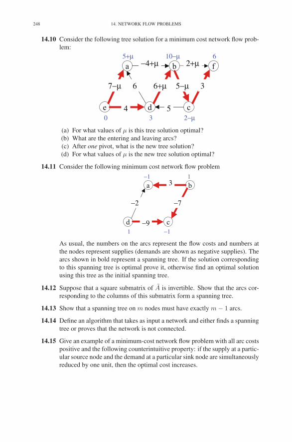
248 14. NETWORK FLOW PROBLEMS
14.10 Consider the following tree solution for a minimum cost network flow prob-
lem:
a
e d
b
c
f
7−µ
−4+µ
6
4 5
6+µ 5−µ 3
2+µ
0 3 2−µ
5+µ 10−µ 6
(a) For what values of μ is this tree solution optimal?
(b) What are the entering and leaving arcs?
(c) After one pivot, what is the new tree solution?
(d) For what values of μ is the new tree solution optimal?
14.11 Consider the following minimum cost network flow problem
a
d c
b
−2
3
−9
−7
1 −1
−1 1
As usual, the numbers on the arcs represent the flow costs and numbers at
the nodes represent supplies (demands are shown as negative supplies). The
arcs shown in bold represent a spanning tree. If the solution corresponding
to this spanning tree is optimal prove it, otherwise find an optimal solution
using this tree as the initial spanning tree.
14.12 Suppose that a square submatrix of A is invertible. Show that the arcs cor-
responding to the columns of this submatrix form a spanning tree.
14.13 Show that a spanning tree on m nodes must have exactly m − 1 arcs.
14.14 Define an algorithm that takes as input a network and either finds a spanning
tree or proves that the network is not connected.
14.15 Give an example of a minimum-cost network flow problem with all arc costs
positive and the following counterintuitive property: if the supply at a partic-
ular source node and the demand at a particular sink node are simultaneously
reduced by one unit, then the optimal cost increases.
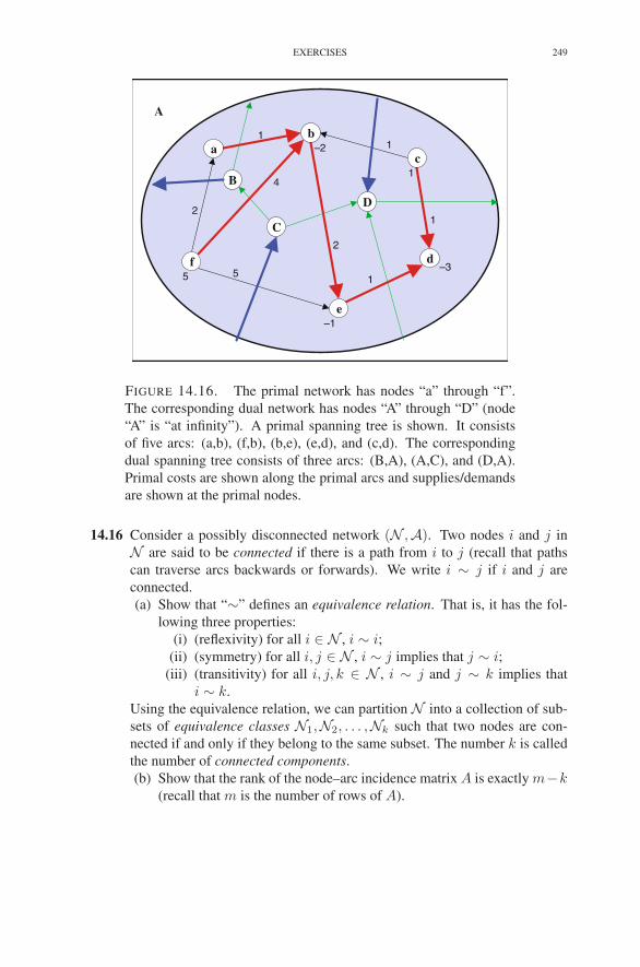
EXERCISES 249
df
e
a
b
c
B
C
D
A
1
11
2
4
2
515
–3
–2
1
–1
FIGURE 14.16. The primal network has nodes “a” through “f”.
The corresponding dual network has nodes “A” through “D” (node
“A” is “at infinity”). A primal spanning tree is shown. It consists
of five arcs: (a,b), (f,b), (b,e), (e,d), and (c,d). The corresponding
dual spanning tree consists of three arcs: (B,A), (A,C), and (D,A).
Primal costs are shown along the primal arcs and supplies/demands
are shown at the primal nodes.
14.16 Consider a possibly disconnected network (N ,A). Two nodes i and j in
N are said to be connected if there is a path from i to j (recall that paths
can traverse arcs backwards or forwards). We write i ∼ j if i and j are
connected.
(a) Show that “∼” defines an equivalence relation. That is, it has the fol-
lowing three properties:
(i) (reflexivity) for all i ∈ N , i ∼ i;(ii) (symmetry) for all i, j ∈ N , i ∼ j implies that j ∼ i;
(iii) (transitivity) for all i, j, k ∈ N , i ∼ j and j ∼ k implies that
i ∼ k.
Using the equivalence relation, we can partition N into a collection of sub-
sets of equivalence classes N1,N2, . . . ,Nk such that two nodes are con-
nected if and only if they belong to the same subset. The number k is called
the number of connected components.
(b) Show that the rank of the node–arc incidence matrix A is exactly m−k(recall that m is the number of rows of A).
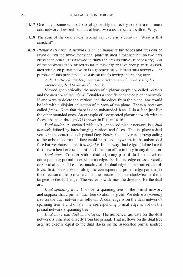
250 14. NETWORK FLOW PROBLEMS
14.17 One may assume without loss of generality that every node in a minimum
cost network flow problem has at least two arcs associated with it. Why?
14.18 The sum of the dual slacks around any cycle is a constant. What is that
constant?
14.19 Planar Networks. A network is called planar if the nodes and arcs can be
layed out on the two-dimensional plane in such a manner that no two arcs
cross each other (it is allowed to draw the arcs as curves if necessary). All
of the networks encountered so far in this chapter have been planar. Associ-
ated with each planar network is a geometrically defined dual network. The
purpose of this problem is to establish the following interesting fact:
A dual network simplex pivot is precisely a primal network simplex
method applied to the dual network.
Viewed geometrically, the nodes of a planar graph are called vertices
and the arcs are called edges. Consider a specific connected planar network.
If one were to delete the vertices and the edges from the plane, one would
be left with a disjoint collection of subsets of the plane. These subsets are
called faces. Note that there is one unbounded face. It is a face just like
the other bounded ones. An example of a connected planar network with its
faces labeled A through D is shown in Figure 14.16.
Dual nodes. Associated with each connected planar network is a dual
network defined by interchanging vertices and faces. That is, place a dual
vertex in the center of each primal face. Note: the dual vertex corresponding
to the unbounded primal face could be placed anywhere in the unbounded
face but we choose to put it at infinity. In this way, dual edges (defined next)
that have a head or a tail at this node can run off to infinity in any direction.
Dual arcs. Connect with a dual edge any pair of dual nodes whose
corresponding primal faces share an edge. Each dual edge crosses exactly
one primal edge. The directionality of the dual edge is determined as fol-
lows: first, place a vector along the corresponding primal edge pointing in
the direction of the primal arc, and then rotate it counterclockwise until it is
tangent to the dual edge. The vector now defines the direction for the dual
arc.
Dual spanning tree. Consider a spanning tree on the primal network
and suppose that a primal–dual tree solution is given. We define a spanning
tree on the dual network as follows. A dual edge is on the dual network’s
spanning tree if and only if the corresponding primal edge is not on the
primal network’s spanning tree.
Dual flows and dual dual-slacks. The numerical arc data for the dual
network is inherited directly from the primal. That is, flows on the dual tree
arcs are exactly equal to the dual slacks on the associated primal nontree
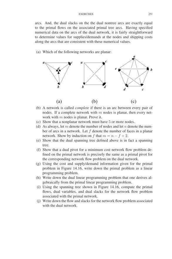
EXERCISES 251
arcs. And, the dual slacks on the the dual nontree arcs are exactly equal
to the primal flows on the associated primal tree arcs. Having specified
numerical data on the arcs of the dual network, it is fairly straightforward
to determine values for supplies/demands at the nodes and shipping costs
along the arcs that are consistent with these numerical values.
(a) Which of the following networks are planar:a
be
d c
aa
bb
cc
d
d
(a) (b) (c)
(b) A network is called complete if there is an arc between every pair of
nodes. If a complete network with m nodes is planar, then every net-
work with m nodes is planar. Prove it.
(c) Show that a nonplanar network must have 5 or more nodes.
(d) As always, let m denote the number of nodes and let n denote the num-
ber of arcs in a network. Let f denote the number of faces in a planar
network. Show by induction on f that m = n − f + 2.
(e) Show that the dual spanning tree defined above is in fact a spanning
tree.
(f) Show that a dual pivot for a minimum cost network flow problem de-
fined on the primal network is precisely the same as a primal pivot for
the corresponding network flow problem on the dual network.
(g) Using the cost and supply/demand information given for the primal
problem in Figure 14.16, write down the primal problem as a linear
programming problem.
(h) Write down the dual linear programming problem that one derives al-
gebraically from the primal linear programming problem.
(i) Using the spanning tree shown in Figure 14.16, compute the primal
flows, dual variables, and dual slacks for the network flow problem
associated with the primal network.
(j) Write down the flow and slacks for the network flow problem associated
with the dual network.

252 14. NETWORK FLOW PROBLEMS
(k) Find arc costs and node supplies/demands for the dual network that are
consistent with the flows and slacks just computed.
(l) Write down the linear programming problem associated with the net-
work flow problem on the dual network.
Notes
The classical reference is Ford & Fulkerson (1962). More recent works include
the books by Christofides (1975), Lawler (1976), Bazaraa et al. (1977), Kennington &
Helgason (1980), Jensen & Barnes (1980), Bertsekas (1991), and Ahuja et al. (1993).
The two “original” algorithms for solving minimum-cost network flow problems
are the network simplex method developed by Dantzig (1951a) and the primal–dual
method developed by Ford & Fulkerson (1958). The self-dual algorithm described
in this chapter is neither of these. In fact, it resembles the “out-of-kilter” method
described by Ford & Fulkerson (1962).

CHAPTER 15
Applications
In this chapter, we discuss briefly the most important applications of network flow
problems.
1. The Transportation Problem
The network flow problem, when thought of as representing the shipment of goods
along a transportation network, is called the transshipment problem. An important
special case is when the set of nodes N can be partitioned into two sets S and D,
N = S ∪ D, S ∩ D = ∅,such that every arc in A has its tail in S and its head in D. The nodes in S are called
source (or supply) nodes, while those in D are called destination (or demand) nodes.
Such graphs are called bipartite graphs (see Figure 15.1). A network flow problem on
such a bipartite graph is called a transportation problem. In order for a transportation
Supplynodes
Demandnodes
FIGURE 15.1. A bipartite graph—the network for a transportation problem.
253
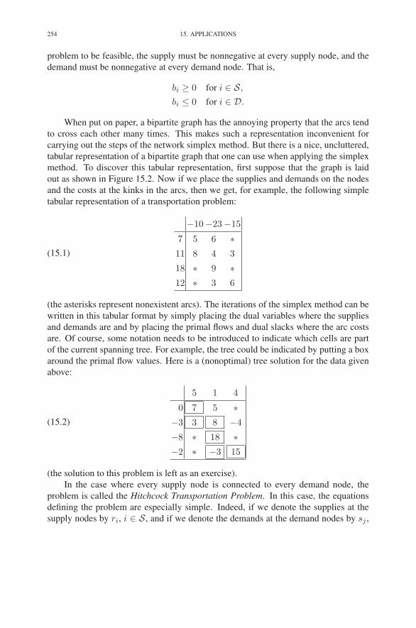
254 15. APPLICATIONS
problem to be feasible, the supply must be nonnegative at every supply node, and the
demand must be nonnegative at every demand node. That is,
bi ≥ 0 for i ∈ S,
bi ≤ 0 for i ∈ D.
When put on paper, a bipartite graph has the annoying property that the arcs tend
to cross each other many times. This makes such a representation inconvenient for
carrying out the steps of the network simplex method. But there is a nice, uncluttered,
tabular representation of a bipartite graph that one can use when applying the simplex
method. To discover this tabular representation, first suppose that the graph is laid
out as shown in Figure 15.2. Now if we place the supplies and demands on the nodes
and the costs at the kinks in the arcs, then we get, for example, the following simple
tabular representation of a transportation problem:
(15.1)
−10−23−15
7 5 6 ∗11 8 4 3
18 ∗ 9 ∗12 ∗ 3 6
(the asterisks represent nonexistent arcs). The iterations of the simplex method can be
written in this tabular format by simply placing the dual variables where the supplies
and demands are and by placing the primal flows and dual slacks where the arc costs
are. Of course, some notation needs to be introduced to indicate which cells are part
of the current spanning tree. For example, the tree could be indicated by putting a box
around the primal flow values. Here is a (nonoptimal) tree solution for the data given
above:
(15.2)
5 1 4
0 7 5 ∗−3 3 8 −4
−8 ∗ 18 ∗−2 ∗ −3 15
(the solution to this problem is left as an exercise).
In the case where every supply node is connected to every demand node, the
problem is called the Hitchcock Transportation Problem. In this case, the equations
defining the problem are especially simple. Indeed, if we denote the supplies at the
supply nodes by ri, i ∈ S, and if we denote the demands at the demand nodes by sj ,

2. THE ASSIGNMENT PROBLEM 255
Supplies
Demands
7
11
18
12
−10 −23 −15
5 6
8 4 3
9
3 6
FIGURE 15.2. The bipartite graph from Figure 15.1 laid out in a
rectangular fashion, with supplies and demands given at the nodes,
and with costs given on the arcs.
j ∈ D, then we can write the problem as
minimize∑
i∈S
∑
j∈Dcijxij
subject to∑
j∈Dxij = ri i ∈ S
∑
i∈Sxij = sj j ∈ D
xij ≥ 0 i ∈ S, j ∈ D.
2. The Assignment Problem
Given a set S of m people, a set D of m tasks, and for each i ∈ S, j ∈ D a cost
cij associated with assigning person i to task j, the assignment problem is to assign
each person to one and only one task in such a manner that each task gets covered by
someone and the total cost of the assignments is minimized. If we let
xij =
{
1 if person i is assigned task j,
0 otherwise,
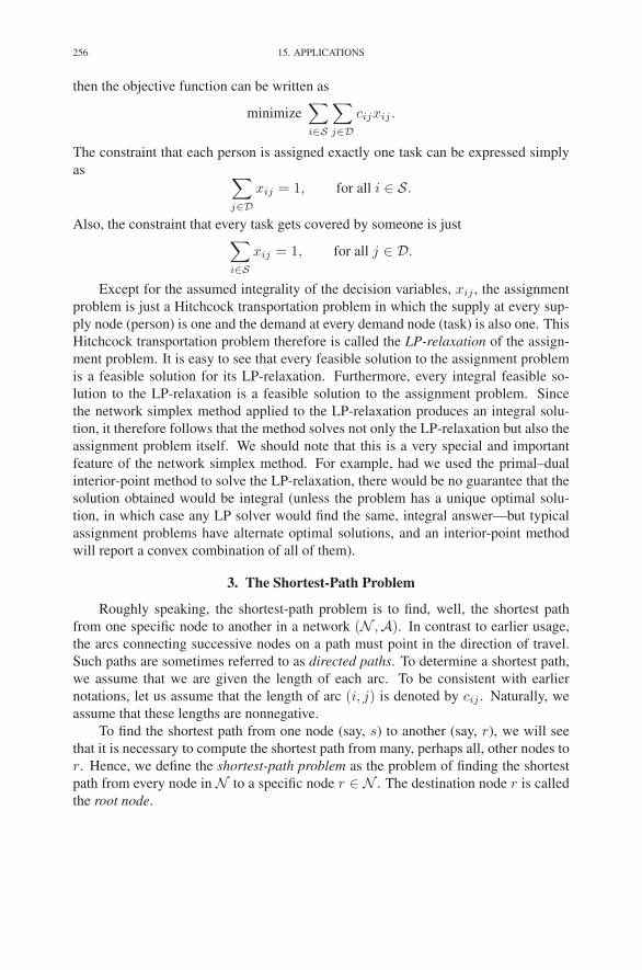
256 15. APPLICATIONS
then the objective function can be written as
minimize∑
i∈S
∑
j∈Dcijxij .
The constraint that each person is assigned exactly one task can be expressed simply
as∑
j∈Dxij = 1, for all i ∈ S.
Also, the constraint that every task gets covered by someone is just∑
i∈Sxij = 1, for all j ∈ D.
Except for the assumed integrality of the decision variables, xij , the assignment
problem is just a Hitchcock transportation problem in which the supply at every sup-
ply node (person) is one and the demand at every demand node (task) is also one. This
Hitchcock transportation problem therefore is called the LP-relaxation of the assign-
ment problem. It is easy to see that every feasible solution to the assignment problem
is a feasible solution for its LP-relaxation. Furthermore, every integral feasible so-
lution to the LP-relaxation is a feasible solution to the assignment problem. Since
the network simplex method applied to the LP-relaxation produces an integral solu-
tion, it therefore follows that the method solves not only the LP-relaxation but also the
assignment problem itself. We should note that this is a very special and important
feature of the network simplex method. For example, had we used the primal–dual
interior-point method to solve the LP-relaxation, there would be no guarantee that the
solution obtained would be integral (unless the problem has a unique optimal solu-
tion, in which case any LP solver would find the same, integral answer—but typical
assignment problems have alternate optimal solutions, and an interior-point method
will report a convex combination of all of them).
3. The Shortest-Path Problem
Roughly speaking, the shortest-path problem is to find, well, the shortest path
from one specific node to another in a network (N ,A). In contrast to earlier usage,
the arcs connecting successive nodes on a path must point in the direction of travel.
Such paths are sometimes referred to as directed paths. To determine a shortest path,
we assume that we are given the length of each arc. To be consistent with earlier
notations, let us assume that the length of arc (i, j) is denoted by cij . Naturally, we
assume that these lengths are nonnegative.
To find the shortest path from one node (say, s) to another (say, r), we will see
that it is necessary to compute the shortest path from many, perhaps all, other nodes to
r. Hence, we define the shortest-path problem as the problem of finding the shortest
path from every node in N to a specific node r ∈ N . The destination node r is called
the root node.

3. THE SHORTEST-PATH PROBLEM 257
3.1. Network Flow Formulation. The shortest-path problem can be formulated
as a network flow problem. Indeed, put a supply of one unit at each nonroot node, and
put the appropriate amount of demand at the root (to meet the total supply). The cost
on each arc is just the length of the arc. Suppose that we’ve solved this network flow
problem. Then the shortest path from a node i to r can be found by simply following
the arcs from i to r on the optimal spanning tree. Also, the length of the shortest path
is y∗r − y∗
i .
While the network simplex method can be used to solve the shortest-path problem,
there are faster algorithms designed especially for it. To describe these algorithms, let
us denote the distance from i to r by vi. These distances (or approximations thereof)
are called labels in the networks literature. Some algorithms compute these distances
systematically in a certain order. These algorithms are called label-setting algorithms.
Other algorithms start with an estimate for these labels and then iteratively correct
the estimates until the optimal values are found. Such algorithms are called label-
correcting algorithms.
Note that if we set y∗r to zero in the network flow solution, then the labels are
simply the negative of the optimal dual variables. In the following subsections, we
shall describe simple examples of label-setting and label-correcting algorithms.
3.2. A Label-Correcting Algorithm. To describe a label-correcting algorithm,
we need to identify a system of equations that characterize the shortest-path distances.
First of all, clearly
vr = 0.
What can we say about the labels at other nodes, say, node i? Suppose that we select
an arc (i, j) that leaves node i. If we were to travel along this arc and then, from node
j, travel along the shortest path to r, then the distance to the root would be cij +vj . So,
from node i, we should select the arc that minimizes these distances. This selection
will then give the shortest distance from i to r. That is,
(15.3) vi = min{cij + vj : (i, j) ∈ A}, i �= r.
The argument we have just made is called the principle of dynamic programming,
and equation (15.3) is called Bellman’s equation. Dynamic programming is a whole
subject of its own—we shall only illustrate some of its basic ideas by our study of the
shortest-path problem. In the dynamic programming literature, the set of vi’s viewed
as a function defined on the nodes is called the value function (hence the notation).
From Bellman’s equation, it is easy to identify the arcs one would travel on in a
shortest-path route to the root. Indeed, these arcs are given by
T = {(i, j) ∈ A : vi = cij + vj}.This set of arcs may contain alternate shortest paths to the root, and so the set is not
necessarily a tree. Nonetheless, any path that follows these arcs will get to the root on
a shortest-path route.
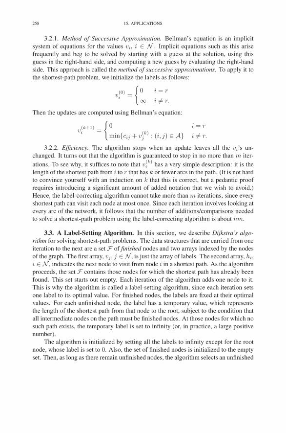
258 15. APPLICATIONS
3.2.1. Method of Successive Approximation. Bellman’s equation is an implicit
system of equations for the values vi, i ∈ N . Implicit equations such as this arise
frequently and beg to be solved by starting with a guess at the solution, using this
guess in the right-hand side, and computing a new guess by evaluating the right-hand
side. This approach is called the method of successive approximations. To apply it to
the shortest-path problem, we initialize the labels as follows:
v(0)i =
{
0 i = r
∞ i �= r.
Then the updates are computed using Bellman’s equation:
v(k+1)i =
{
0 i = r
min{cij + v(k)j : (i, j) ∈ A} i �= r.
3.2.2. Efficiency. The algorithm stops when an update leaves all the vi’s un-
changed. It turns out that the algorithm is guaranteed to stop in no more than m iter-
ations. To see why, it suffices to note that v(k)i has a very simple description: it is the
length of the shortest path from i to r that has k or fewer arcs in the path. (It is not hard
to convince yourself with an induction on k that this is correct, but a pedantic proof
requires introducing a significant amount of added notation that we wish to avoid.)
Hence, the label-correcting algorithm cannot take more than m iterations, since every
shortest path can visit each node at most once. Since each iteration involves looking at
every arc of the network, it follows that the number of additions/comparisons needed
to solve a shortest-path problem using the label-correcting algorithm is about nm.
3.3. A Label-Setting Algorithm. In this section, we describe Dijkstra’s algo-
rithm for solving shortest-path problems. The data structures that are carried from one
iteration to the next are a set F of finished nodes and two arrays indexed by the nodes
of the graph. The first array, vj , j ∈ N , is just the array of labels. The second array, hi,
i ∈ N , indicates the next node to visit from node i in a shortest path. As the algorithm
proceeds, the set F contains those nodes for which the shortest path has already been
found. This set starts out empty. Each iteration of the algorithm adds one node to it.
This is why the algorithm is called a label-setting algorithm, since each iteration sets
one label to its optimal value. For finished nodes, the labels are fixed at their optimal
values. For each unfinished node, the label has a temporary value, which represents
the length of the shortest path from that node to the root, subject to the condition that
all intermediate nodes on the path must be finished nodes. At those nodes for which no
such path exists, the temporary label is set to infinity (or, in practice, a large positive
number).
The algorithm is initialized by setting all the labels to infinity except for the root
node, whose label is set to 0. Also, the set of finished nodes is initialized to the empty
set. Then, as long as there remain unfinished nodes, the algorithm selects an unfinished

4. UPPER-BOUNDED NETWORK FLOW PROBLEMS 259
Initialize:
F = ∅
vj =
{
0 j = r,
∞ j �= r.
while (|Fc| > 0){j = argmin{vk : k �∈ F}F ← F ∪ {j}for each i for which (i, j) ∈ A and i �∈ F {
if (cij + vj < vi) {vi = cij + vj
hi = j
}}
}
FIGURE 15.3. Dijkstra’s shortest-path algorithm.
node j having the smallest temporary label, adds it to the set of finished nodes, and
then updates each unfinished “upstream” neighbor i by setting its label to cij + vj if
this value is smaller than the current value vi. For each neighbor i whose label gets
changed, hi is set to j. The algorithm is summarized in Figure 15.3.
4. Upper-Bounded Network Flow Problems
Some real-world network flow problems involve upper bounds on the amount
of flow that an arc can handle. There are modified versions of the network simplex
method that allow one to handle such upper bounds implicitly, but we shall simply
show how to reduce an upper-bounded network flow problem to one without upper
bounds.
Let us consider just one arc, (i, j), in a network flow problem. Suppose that there
is an upper bound of uij on the amount of flow that this arc can handle. We can express
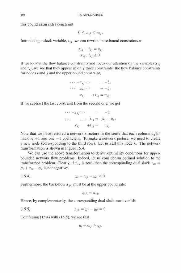
260 15. APPLICATIONS
this bound as an extra constraint:
0 ≤ xij ≤ uij .
Introducing a slack variable, tij , we can rewrite these bound constraints as
xij + tij = uij
xij , tij ≥ 0.
If we look at the flow balance constraints and focus our attention on the variables xij
and tij , we see that they appear in only three constraints: the flow balance constraints
for nodes i and j and the upper bound constraint,
· · · −xij · · · = −bi
· · · xij · · · =−bj
xij +tij = uij .
If we subtract the last constraint from the second one, we get
· · · −xij · · · = −bi
· · · · · · −tij =−bj − uij
xij +tij = uij .
Note that we have restored a network structure in the sense that each column again
has one +1 and one −1 coefficient. To make a network picture, we need to create
a new node (corresponding to the third row). Let us call this node k. The network
transformation is shown in Figure 15.4.
We can use the above transformation to derive optimality conditions for upper-
bounded network flow problems. Indeed, let us consider an optimal solution to the
transformed problem. Clearly, if xik is zero, then the corresponding dual slack zik =yi + cij − yk is nonnegative:
(15.4) yi + cij − yk ≥ 0.
Furthermore, the back-flow xjk must be at the upper bound rate:
xjk = uij .
Hence, by complementarity, the corresponding dual slack must vanish:
(15.5) zjk = yj − yk = 0.
Combining (15.4) with (15.5), we see that
yi + cij ≥ yj .
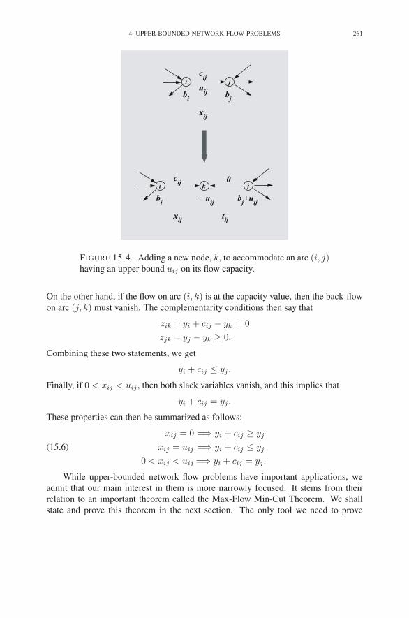
4. UPPER-BOUNDED NETWORK FLOW PROBLEMS 261
i j
bi
cij
bj
uij
xij
ki j
bi
−uij
cij 0
bj+uij
xij
tij
FIGURE 15.4. Adding a new node, k, to accommodate an arc (i, j)having an upper bound uij on its flow capacity.
On the other hand, if the flow on arc (i, k) is at the capacity value, then the back-flow
on arc (j, k) must vanish. The complementarity conditions then say that
zik = yi + cij − yk = 0
zjk = yj − yk ≥ 0.
Combining these two statements, we get
yi + cij ≤ yj .
Finally, if 0 < xij < uij , then both slack variables vanish, and this implies that
yi + cij = yj .
These properties can then be summarized as follows:
xij = 0 =⇒ yi + cij ≥ yj
xij = uij =⇒ yi + cij ≤ yj(15.6)
0 < xij < uij =⇒ yi + cij = yj .
While upper-bounded network flow problems have important applications, we
admit that our main interest in them is more narrowly focused. It stems from their
relation to an important theorem called the Max-Flow Min-Cut Theorem. We shall
state and prove this theorem in the next section. The only tool we need to prove
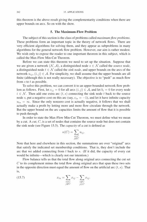
262 15. APPLICATIONS
this theorem is the above result giving the complementarity conditions when there are
upper bounds on arcs. So on with the show.
5. The Maximum-Flow Problem
The subject of this section is the class of problems called maximum-flow problems.
These problems form an important topic in the theory of network flows. There are
very efficient algorithms for solving them, and they appear as subproblems in many
algorithms for the general network flow problem. However, our aim is rather modest.
We wish only to expose the reader to one important theorem in this subject, which is
called the Max-Flow Min-Cut Theorem.
Before we can state this theorem we need to set up the situation. Suppose that
we are given a network (N ,A), a distinguished node s ∈ N called the source node,
a distinguished node t ∈ N called the sink node, and upper bounds on the arcs of the
network uij , (i, j) ∈ A. For simplicity, we shall assume that the upper bounds are all
finite (although this is not really necessary). The objective is to “push” as much flow
from s to t as possible.
To solve this problem, we can convert it to an upper-bounded network flow prob-
lem as follows. First, let cij = 0 for all arcs (i, j) ∈ A, and let bi = 0 for every node
i ∈ N . Then add one extra arc (t, s) connecting the sink node t back to the source
node s, put a negative cost on this arc (say, cts = −1), and let it have infinite capacity
uts = ∞. Since the only nonzero cost is actually negative, it follows that we shall
actually make a profit by letting more and more flow circulate through the network.
But the upper bound on the arc capacities limits the amount of flow that it is possible
to push through.
In order to state the Max-Flow Min-Cut Theorem, we must define what we mean
by a cut. A cut, C, is a set of nodes that contains the source node but does not contain
the sink node (see Figure 15.5). The capacity of a cut is defined as
κ(C) =∑
i∈Cj ∈C
uij .
Note that here and elsewhere in this section, the summations are over “original” arcs
that satisfy the indicated set membership conditions. That is, they don’t include the
arc that we added connecting from t back to s. (If it did, the capacity of every cut
would be infinite—which is clearly not our intention.)
Flow balance tells us that the total flow along original arcs connecting the cut set
C to its complement minus the total flow along original arcs that span these two sets
in the opposite direction must equal the amount of flow on the artificial arc (t, s). That
is,
(15.7) xts =∑
i∈Cj ∈C
xij −∑
i∈Cj∈C
xij .

5. THE MAXIMUM-FLOW PROBLEM 263
s
t
C
cts
= −1
FIGURE 15.5. A cut set C for a maximum flow problem.
We are now ready to state the Max-Flow Min-Cut Theorem.
THEOREM 15.1. The maximum value of xts equals the minimum value of κ(C).
PROOF. The proof follows the usual sort of pattern common in subjects where
there is a sort of duality theory. First of all, we note that it follows from (15.7) that
(15.8) xts ≤ κ(C)
for every feasible flow and every cut set C. Then all that is required is to exhibit a
feasible flow and a cut set for which this inequality is an equality.
Let x∗ij , (i, j) ∈ A, denote the optimal values of the primal variables, and let y∗
i ,
i ∈ N , denote the optimal values of the dual variables. Then the complementarity
conditions (15.6) imply that
x∗ij = 0 whenever y∗
i + cij > y∗j(15.9)
x∗ij = uij whenever y∗
i + cij < y∗j .(15.10)
In particular,
y∗t − 1 ≥ y∗
s
(since uts = ∞). Put C∗ = {k : y∗k ≤ y∗
s}. Clearly, C∗ is a cut.
Consider an arc having its tail in C∗ and its head in the complement of C∗. It
follows from the definition of C∗ that y∗i ≤ y∗
s < y∗j . Since cij is zero, we see from
(15.10) that x∗ij = uij .
Now consider an original arc having its tail in the complement of C∗ and its
head in C∗ (i.e., bridging the two sets in the opposite direction). It follows then that
y∗j ≤ y∗
s < y∗i . Hence, we see from (15.9) that x∗
ij = 0.
264 15. APPLICATIONS
Combining the observations of the last two paragraphs with (15.7), we see that
x∗ts =
∑
i∈Cj ∈C
uij = κ(C∗).
In light of (15.8), the proof is complete. �
Exercises
15.1 Solve the transportation problem given in (15.1), using (15.2) for the starting
tree solution.
15.2 Solve the following linear programming problem:
maximize 7x1 − 3x2 + 9x3 + 2x4
subject to x1 + x2 ≤ 1
x3 + x4 ≤ 1
x1 + x3 ≥ 1
x2 + x4 ≥ 1
x1, x2, x3, x4 ≥ 0.
(Note: there are two greater-than-or-equal-to constraints.)
15.3 Bob, Carol, David, and Alice are stranded on a desert island. Bob and David
each would like to give their affection to Carol or to Alice. Food is the
currency of trade for this starving foursome. Bob is willing to pay Carol 7clams if she will accept his affection. David is even more keen and is willing
to give Carol 9 clams if she will accept it. Both Bob and David prefer Carol
to Alice (sorry Alice). To quantify this preference, David is willing to pay
Alice only 2 clams for his affection. Bob is even more averse: he says that
Alice would have to pay him for it. In fact, she’d have to pay him 3 clams
for his affection. Carol and Alice, being proper young women, will accept
affection from one and only one of the two guys. Between the two of them
they have decided to share the clams equally between them and hence their
objective is simply to maximize the total number of clams they will receive.
Formulate this problem as a transportation problem. Solve it.
15.4 Project Scheduling. This problem deals with the creation of a project sched-
ule; specifically, the project of building a house. The project has been di-
vided into a set of jobs. The problem is to schedule the time at which each
of these jobs should start and also to predict how long the project will take.
Naturally, the objective is to complete the project as quickly as possible
(time is money!). Over the duration of the project, some of the jobs can be

EXERCISES 265
done concurrently. But, as the following table shows, certain jobs definitely
can’t start until others are completed.
Duration Must be
Job (weeks) Preceeded by
0. Sign Contract with Buyer 0 –
1. Framing 2 0
2. Roofing 1 1
3. Siding 3 1
4. Windows 2.5 3
5. Plumbing 1.5 3
6. Electical 2 2,4
7. Inside Finishing 4 5,6
8. Outside Painting 3 2,4
9. Complete the Sale to Buyer 0 7,8
One possible schedule is the following:
Job Start Time
0. Sign Contract with Buyer 0
1. Framing 1
2. Roofing 4
3. Siding 6
4. Windows 10
5. Plumbing 9
6. Electical 13
7. Inside Finishing 16
8. Outside Painting 14
9. Complete the Sale to Buyer 21
With this schedule, the project duration is 21 weeks (the difference be-
tween the start times of jobs 9 and 0).
To model the problem as a linear program, introduce the following de-
cision variables:
tj = the start time of job j.

266 15. APPLICATIONS
(a) Write an expression for the objective function, which is to minimize the
project duration.
(b) For each job j, write a constraint for each job i that must preceed j; the
constraint should ensure that job j doesn’t start until job i is finished.
These are called precedence constraints.
15.5 Continuation. This problem generalizes the specific example of the previous
problem. A project consists of a set of jobs J . For each job j ∈ J there
is a certain set Pj of other jobs that must be completed before job j can be
started. (This is called the set of predecessors of job j.) One of the jobs, say
s, is the starting job; it has no predecessors. Another job, say t, is the final
(or terminal) job; it is not the predecessor of any other job. The time it will
take to do job j is denoted dj (the duration of the job).
The problem is to decide what time each job should begin so that no
job begins before its predecessors are finished, and the duration of the entire
project is minimized. Using the notations introduced above, write out a
complete description of this linear programming problem.
15.6 Continuation. Let xij denote the dual variable corresponding to the prece-
dence constraint that ensures job j doesn’t start until job i finishes.
(a) Write out the dual to the specific linear program in Problem 15.4.
(b) Write out the dual to the general linear program in Problem 15.5.
(c) Describe how the optimal value of the dual variable xij can be inter-
preted.
15.7 Continuation. The project scheduling problem can be represented on a di-
rected graph with arc weights as follows. The nodes of the graph correspond
to the jobs. The arcs correspond to the precedence relations. That is, if job imust be completed before job j, then there is an arc pointing from node i to
node j. The weight on this arc is di.
(a) Draw the directed graph associated with the example in Problem 15.4,
being sure to label the nodes and write the weights beside the arcs.
(b) Return to the formulation of the dual from Problem 15.6(a). Give an
interpretation of that dual problem in terms of the directed graph drawn
in Part (a).
(c) Explain why there is always an optimal solution to the dual problem in
which each variable xij is either 0 or 1.
(d) Write out the complementary slackness condition corresponding to dual
variable x26.

EXERCISES 267
(e) Describe the dual problem in the language of the original project sched-
uling model.
15.8 Continuation. Here is an algorithm for computing optimal start times tj :
1. List the jobs so that the predecessors of each job come be-
fore it in the list.
2. Put t0 = 0.
3. Go down the list of jobs and for job j put tj = max{ti+di :i is a predecessor of j}.
(a) Apply this algorithm to the specific instance from Problem 15.4. What
are the start times of each of the jobs? What is the project duration?
(b) Prove that the solution found in Part (a) is optimal by exhibiting a corre-
sponding dual solution and checking the usual conditions for optimal-
ity (Hint: The complementary slackness conditions may help you find a
dual solution.).
15.9 Currency Arbitrage. Consider the world’s currency market. Given two cur-
rencies, say the Japanese Yen and the US Dollar, there is an exchange rate
between them (currently about 110 Yen to the Dollar). It is always true that,
if you convert money from one currency to another and then back, you will
end up with less than you started with. That is, the product of the exchange
rates between any pair of countries is always less than one. However, it
sometimes happens that a longer chain of conversions results in a gain. Such
a lucky situation is called an arbitrage. One can use a linear programming
model to find such situations when they exist.
Consider the following table of exchange rates (which is actual data
from the Wall Street Journal on Nov 10, 1996):
param rate:USD Yen Mark Franc :=
USD . 111.52 1.4987 5.0852Yen .008966 . .013493 .045593Mark .6659 73.964 . 3.3823Franc .1966 21.933 .29507 .;
It is not obvious, but the USD→Yen→Mark→USD conversion actually makes
$0.002 on each initial dollar.
268 15. APPLICATIONS
To look for arbitrage possibilities, one can make a generalized network
model, which is a network flow model with the unusual twist that a unit
of flow that leaves one node arrives at the next node multiplied by a scale
factor—in our example, the currency conversion rate. For us, each currency
is represented by a node. There is an arc from each node to every other node.
A flow of one unit out of one node becomes a flow of a different magnitude
at the head node. For example, one dollar flowing out of the USD node
arrives at the Franc node as 5.0852 Francs.
Let xij denote the flow from node (i.e. currency) i to node j. This flow
is measured in the currency of node i.One node is special; it is the home node, say the US Dollars (USD)
node. At all other nodes, there must be flow balance.
(a) Write down the flow balance constraints at the 3 non-home nodes (Franc,
Yen, and Mark).
At the home node, we assume that there is a supply of one unit (to get things
started). Furthermore, at this node, flow balance will not be satisfied. Instead
one expects a net inflow. If it is possible to make this inflow greater than
one, then an arbitrage has been found. Let f be a variable that represents
this inflow.
(b) Using variable f to represent net inflow to the home node, write a flow
balance equation for the home node.
Of course, the primal objective is to maximize f .
(c) Using yi to represent the dual variable associated with the primal con-
straint for currency i, write down the dual linear program. (Regard the
primal variable f as a free variable.)
Now consider the general case, which might involve hundreds of currencies
worldwide.
(d) Write down the model mathematically using xij for the flow leaving
node i heading for node j (measured in the currency of node i), rij for
the exchange rate when converting from currency i to currency j, and
f for the net inflow at the home node i∗.
(e) Write down the dual problem.

NOTES 269
(f) Can you give an interpretation for the dual variables? Hint: It might be
helpful to think about the case where rji = 1/rij for all i, j.
(g) Comment on the conditions under which your model will be unbounded
and/or infeasible.
Notes
The Hitchcock problem was introduced by Hitchcock (1941). Dijkstra’s algo-
rithm was discovered by Dijkstra (1959).
The Max-Flow Min-Cut Theorem was proved independently by Elias et al. (1956),
by Ford & Fulkerson (1956) and, in the restricted case where the upper bounds are all
integers, by Kotzig (1956). Fulkerson & Dantzig (1955) also proved the Max-Flow
Min-Cut Theorem. Their proof uses duality, which is particularly relevant to this
chapter.
The classic references for dynamic programming are the books by Bellman (1957)
and Howard (1960). Further discussion of label-setting and label-correcting algo-
rithms can be found in the book by Ahuja et al. (1993).


CHAPTER 16
Structural Optimization
This final chapter on network-type problems deals with finding the best design
of a structure to support a specified load at a fixed set of points. The topology of the
problem is described by a graph where each node represents a joint in the structure and
each arc represents a potential member.1 We shall formulate this problem as a linear
programming problem whose solution determines which of the potential members to
include in the structure and how thick each included member must be to handle the
load. The optimization criterion is to find a minimal weight structure. As we shall see,
the problem bears a striking resemblance to the minimum-cost network flow problem
that we studied in Chapter 14.
1. An Example
We begin with an example. Consider the graph shown in Figure 16.1. This graph
represents a structure consisting of five joints and eight possible members connecting
the joints. The five joints and their coordinates are given as follows:
Joint Coordinates
1 (0.0 , 0.0)
2 (6.0 , 0.0)
3 (0.0 , 8.0)
4 (6.0 , 8.0)
5 (3.0 , 12.0)
Since joints are analogous to nodes in a network, we shall denote the set of joints by
N and denote by m the number of joints. Also, since members are analogous to arcs
in network flows, we shall denote the set of them by A. For the structure shown in
Figure 16.1, the set of members is
A = {{1, 2}, {1, 3}, {1, 4}, {2, 3}, {2, 4}, {3, 4}, {3, 5}, {4, 5}} .
1Civil engineers refer to beams as members.
271
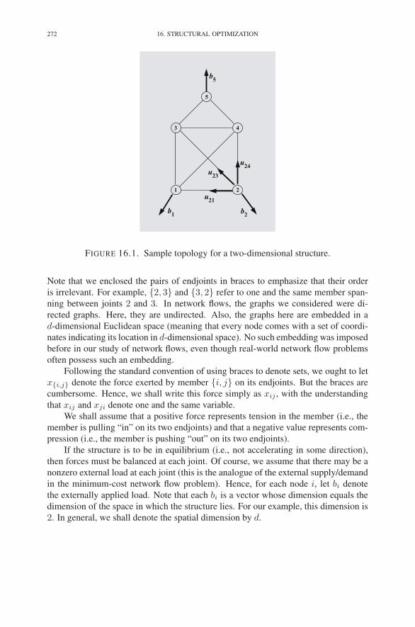
272 16. STRUCTURAL OPTIMIZATION
3
1 2
4
5
b1
b2
b5
u21
u24
u23
FIGURE 16.1. Sample topology for a two-dimensional structure.
Note that we enclosed the pairs of endjoints in braces to emphasize that their order
is irrelevant. For example, {2, 3} and {3, 2} refer to one and the same member span-
ning between joints 2 and 3. In network flows, the graphs we considered were di-
rected graphs. Here, they are undirected. Also, the graphs here are embedded in a
d-dimensional Euclidean space (meaning that every node comes with a set of coordi-
nates indicating its location in d-dimensional space). No such embedding was imposed
before in our study of network flows, even though real-world network flow problems
often possess such an embedding.
Following the standard convention of using braces to denote sets, we ought to let
x{i,j} denote the force exerted by member {i, j} on its endjoints. But the braces are
cumbersome. Hence, we shall write this force simply as xij , with the understanding
that xij and xji denote one and the same variable.
We shall assume that a positive force represents tension in the member (i.e., the
member is pulling “in” on its two endjoints) and that a negative value represents com-
pression (i.e., the member is pushing “out” on its two endjoints).
If the structure is to be in equilibrium (i.e., not accelerating in some direction),
then forces must be balanced at each joint. Of course, we assume that there may be a
nonzero external load at each joint (this is the analogue of the external supply/demand
in the minimum-cost network flow problem). Hence, for each node i, let bi denote
the externally applied load. Note that each bi is a vector whose dimension equals the
dimension of the space in which the structure lies. For our example, this dimension is
2. In general, we shall denote the spatial dimension by d.

2. INCIDENCE MATRICES 273
Force balance imposes a number of constraints on the member forces. For exam-
ple, the force balance equations for joint 2 can be written as follows:
x12
[
−1
0
]
+ x23
[
−0.6
0.8
]
+ x24
[
0
1
]
= −[
b12
b22
]
,
where b12 and b2
2 denote the components of b2. Note that the three vectors appearing
on the left are unit vectors pointing out from joint 2 along each of the corresponding
members.
2. Incidence Matrices
If, for each joint i, we let pi denote its position vector, then the unit vectors point-
ing along the arcs can be written as follows:
uij =pj − pi
‖pj − pi‖, {i, j} ∈ A.
It is important to note that uji = −uij , since the first vector points from j towards
i, whereas the second points from i towards j. In terms of these notations, the force
balance equations can be expressed succinctly as
(16.1)∑
j:{i,j}∈A
uijxij = −bi i = 1, 2, . . . , m.
These equations can be written in matrix form as
(16.2) Ax = −b
where x denotes the vector consisting of the member forces, b denotes the vector
whose elements are the applied load vectors, and A is a matrix containing the unit
vectors pointing along the appropriate arcs. For our example, we have
xT =[
x12 x13 x14 x23 x24 x34 x35 x45
]
A =
1
2
3
4
5
⎡
⎢
⎢
⎢
⎢
⎢
⎢
⎢
⎢
⎢
⎢
⎢
⎢
⎢
⎢
⎢
⎢
⎢
⎢
⎢
⎢
⎢
⎣
[
1
0
] [
0
1
] [
.6
.8
]
[
−1
0
] [
−.6
.8
] [
0
1
]
[
0
−1
] [
.6
−.8
] [
1
0
] [
.6
.8
]
[
−.6
−.8
] [
0
−1
] [
−1
0
] [
−.6
.8
]
[
−.6
−.8
] [
.6
−.8
]
⎤
⎥
⎥
⎥
⎥
⎥
⎥
⎥
⎥
⎥
⎥
⎥
⎥
⎥
⎥
⎥
⎥
⎥
⎥
⎥
⎥
⎥
⎦
, b =
⎡
⎢
⎢
⎢
⎢
⎢
⎢
⎢
⎢
⎢
⎢
⎢
⎢
⎢
⎢
⎢
⎢
⎢
⎢
⎢
⎢
⎢
⎣
b11
b21
b12
b22
b13
b23
b14
b24
b15
b25
⎤
⎥
⎥
⎥
⎥
⎥
⎥
⎥
⎥
⎥
⎥
⎥
⎥
⎥
⎥
⎥
⎥
⎥
⎥
⎥
⎥
⎥
⎦
.
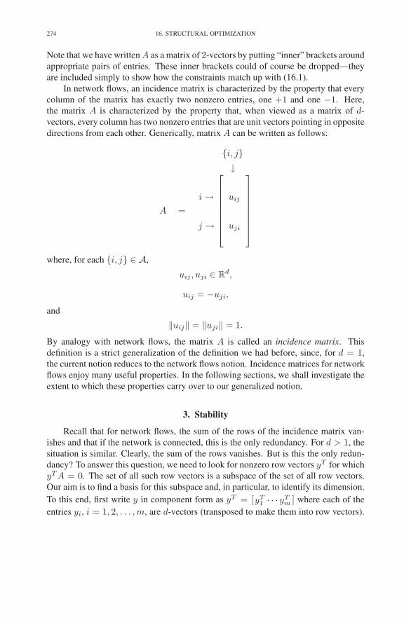
274 16. STRUCTURAL OPTIMIZATION
Note that we have written A as a matrix of 2-vectors by putting “inner” brackets around
appropriate pairs of entries. These inner brackets could of course be dropped—they
are included simply to show how the constraints match up with (16.1).
In network flows, an incidence matrix is characterized by the property that every
column of the matrix has exactly two nonzero entries, one +1 and one −1. Here,
the matrix A is characterized by the property that, when viewed as a matrix of d-
vectors, every column has two nonzero entries that are unit vectors pointing in opposite
directions from each other. Generically, matrix A can be written as follows:
{i, j}↓
A =
i →
j →
⎡
⎢
⎢
⎢
⎢
⎢
⎢
⎢
⎣
uij
uji
⎤
⎥
⎥
⎥
⎥
⎥
⎥
⎥
⎦
where, for each {i, j} ∈ A,
uij , uji ∈ Rd,
uij = −uji,
and
‖uij‖ = ‖uji‖ = 1.
By analogy with network flows, the matrix A is called an incidence matrix. This
definition is a strict generalization of the definition we had before, since, for d = 1,
the current notion reduces to the network flows notion. Incidence matrices for network
flows enjoy many useful properties. In the following sections, we shall investigate the
extent to which these properties carry over to our generalized notion.
3. Stability
Recall that for network flows, the sum of the rows of the incidence matrix van-
ishes and that if the network is connected, this is the only redundancy. For d > 1, the
situation is similar. Clearly, the sum of the rows vanishes. But is this the only redun-
dancy? To answer this question, we need to look for nonzero row vectors yT for which
yT A = 0. The set of all such row vectors is a subspace of the set of all row vectors.
Our aim is to find a basis for this subspace and, in particular, to identify its dimension.
To this end, first write y in component form as yT = [yT1 · · · yT
m ] where each of the
entries yi, i = 1, 2, . . . ,m, are d-vectors (transposed to make them into row vectors).

3. STABILITY 275
Multiplying this row vector against each column of A, we see that yT A = 0 if and
only if
(16.3) yTi uij + yT
j uji = 0, for all {i, j} ∈ A.
There are many choices of y that yield a zero row combination. For example, we can
take any vector v ∈ Rd and put
yi = v, for every i ∈ N .
Substituting this choice of yi’s into the left-hand side of (16.3), we get
yTi uij + yT
j uji = vT uij + vT uji = vT uij − vT uij = 0.
This set of choices shows that the subspace is at least d-dimensional.
But there are more! They are defined in terms of skew symmetric matrices. A
matrix R is called skew symmetric if RT = −R. A simple but important property of
skew symmetric matrices is that, for every vector ξ,
(16.4) ξT Rξ = 0
(see Exercise 16.1). We shall make use of this property shortly. Now, to give more
choices of y, let R be a d × d skew symmetric matrix and put
yi = Rpi, for every i ∈ N
(recall that pi denotes the position vector for joint i). We need to check (16.3). Sub-
stituting this definition of the y’s into the left-hand side in (16.3), we see that
yTi uij + yT
j uji = pTi RT uij + pT
j RT uji
=−pTi Ruij − pT
j Ruji
= (pj − pi)T Ruij .
Now substituting in the definition of uij , we get
(pj − pi)T Ruij =
(pj − pi)T R(pj − pi)
‖pj − pi‖.
Finally, by putting ξ = pj − pi and using property (16.4) of skew symmetric matrices,
we see that the numerator on the right vanishes. Hence, (16.3) holds.
How many redundancies have we found? For d = 2, there are two independent
v-type redundancies and one more R-type. The following two vectors and a matrix
can be taken as a basis for these redundancies[
1
0
]
,
[
0
1
]
,
[
0 −1
1 0
]
.
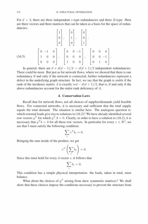
276 16. STRUCTURAL OPTIMIZATION
For d = 3, there are three independent v-type redundancies and three R-type. Here
are three vectors and three matrices that can be taken as a basis for the space of redun-
dancies:⎡
⎢
⎢
⎣
1
0
0
⎤
⎥
⎥
⎦
,
⎡
⎢
⎢
⎣
0
1
0
⎤
⎥
⎥
⎦
,
⎡
⎢
⎢
⎣
0
0
1
⎤
⎥
⎥
⎦
,
(16.5)
⎡
⎢
⎢
⎣
0 −1 0
1 0 0
0 0 0
⎤
⎥
⎥
⎦
,
⎡
⎢
⎢
⎣
0 0 −1
0 0 0
1 0 0
⎤
⎥
⎥
⎦
,
⎡
⎢
⎢
⎣
0 0 0
0 0 −1
0 1 0
⎤
⎥
⎥
⎦
.
In general, there are d + d(d − 1)/2 = d(d + 1)/2 independent redundancies.
There could be more. But just as for network flows, where we showed that there is one
redundancy if and only if the network is connected, further redundancies represent a
defect in the underlying graph structure. In fact, we say that the graph is stable if the
rank of the incidence matrix A is exactly md − d(d + 1)/2, that is, if and only if the
above redundancies account for the entire rank deficiency of A.
4. Conservation Laws
Recall that for network flows, not all choices of supplies/demands yield feasible
flows. For connected networks, it is necessary and sufficient that the total supply
equals the total demand. The situation is similar here. The analogous question is:
which external loads give rise to solutions to (16.2)? We have already identified several
row vectors yT for which yT A = 0. Clearly, in order to have a solution to (16.2), it is
necessary that yT b = 0 for all these row vectors. In particular for every v ∈ Rd, we
see that b must satisfy the following condition:∑
i
vT bi = 0.
Bringing the sum inside of the product, we get
vT
(
∑
i
bi
)
= 0.
Since this must hold for every d-vector v, it follows that∑
i
bi = 0.
This condition has a simple physical interpretation: the loads, taken in total, must
balance.
What about the choices of yT arising from skew symmetric matrices? We shall
show that these choices impose the conditions necessary to prevent the structure from
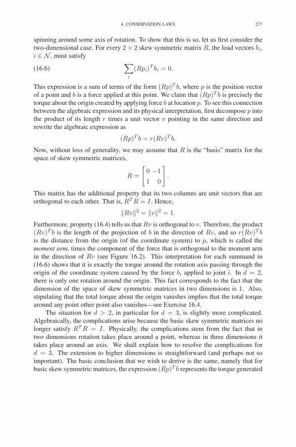
4. CONSERVATION LAWS 277
spinning around some axis of rotation. To show that this is so, let us first consider the
two-dimensional case. For every 2 × 2 skew symmetric matrix R, the load vectors bi,
i ∈ N , must satisfy
(16.6)∑
i
(Rpi)T bi = 0.
This expression is a sum of terms of the form (Rp)T b, where p is the position vector
of a point and b is a force applied at this point. We claim that (Rp)T b is precisely the
torque about the origin created by applying force b at location p. To see this connection
between the algebraic expression and its physical interpretation, first decompose p into
the product of its length r times a unit vector v pointing in the same direction and
rewrite the algebraic expression as
(Rp)T b = r(Rv)T b.
Now, without loss of generality, we may assume that R is the “basis” matrix for the
space of skew symmetric matrices,
R =
[
0 −1
1 0
]
.
This matrix has the additional property that its two columns are unit vectors that are
orthogonal to each other. That is, RT R = I . Hence,
‖Rv‖2 = ‖v‖2 = 1.
Furthermore, property (16.4) tells us that Rv is orthogonal to v. Therefore, the product
(Rv)T b is the length of the projection of b in the direction of Rv, and so r(Rv)T bis the distance from the origin (of the coordinate system) to p, which is called the
moment arm, times the component of the force that is orthogonal to the moment arm
in the direction of Rv (see Figure 16.2). This interpretation for each summand in
(16.6) shows that it is exactly the torque around the rotation axis passing through the
origin of the coordinate system caused by the force bi applied to joint i. In d = 2,
there is only one rotation around the origin. This fact corresponds to the fact that the
dimension of the space of skew symmetric matrices in two dimensions is 1. Also,
stipulating that the total torque about the origin vanishes implies that the total torque
around any point other point also vanishes—see Exercise 16.4.
The situation for d > 2, in particular for d = 3, is slightly more complicated.
Algebraically, the complications arise because the basic skew symmetric matrices no
longer satisfy RT R = I . Physically, the complications stem from the fact that in
two dimensions rotation takes place around a point, whereas in three dimensions it
takes place around an axis. We shall explain how to resolve the complications for
d = 3. The extension to higher dimensions is straightforward (and perhaps not so
important). The basic conclusion that we wish to derive is the same, namely that for
basic skew symmetric matrices, the expression (Rp)T b represents the torque generated

278 16. STRUCTURAL OPTIMIZATION
bi
pi
Rvi
vi
0
i
FIGURE 16.2. The ith summand in (16.6) is the length of pi times
the length of the projection of bi onto the direction given by Rvi.
This is precisely the torque around an axis at 0 caused by the force
bi applied at joint i.
by applying a force b at point p. Recall that there are just three basic skew symmetric
matrices, and they are given by (16.5). To be specific, let us just study the first one:
R =
⎡
⎢
⎢
⎣
0 −1 0
1 0 0
0 0 0
⎤
⎥
⎥
⎦
.
This matrix can be decomposed into the product of two matrices:
R = UP
where
U =
⎡
⎢
⎢
⎣
0 −1 0
1 0 0
0 0 1
⎤
⎥
⎥
⎦
and P =
⎡
⎢
⎢
⎣
1 0 0
0 1 0
0 0 0
⎤
⎥
⎥
⎦
.
The matrix U has the property that R had before, namely,
UT U = I.
Such matrices are called unitary. The matrix P is a projection matrix. If we let
q = Pp,
v =q
‖q‖ ,
and
r = ‖q‖,

5. MINIMUM-WEIGHT STRUCTURAL DESIGN 279
}v
q
p
b
}r
( vU)Tb
x1
x2
x3
vU
FIGURE 16.3. The decomposition of (Rp)T b into the product of a
moment arm r times the component of b in the direction Uv shows
that it is precisely the torque around the third axis.
then we can rewrite (Rp)T b as
(Rp)T b = r(Uv)T b.
Since v is a unit vector and U is unitary, it follows that Uv is a unit vector. Hence,
(Uv)T b represents the scalar projection of b onto the direction determined by Uv.
Also, it is easy to check that Uv is orthogonal to v. At this point, we can consult
Figure 16.3 to see that r is the moment arm for the torque around the third coordinate
axis and (Uv)T b is the component of force in the direction of rotation around this axis.
Therefore, the product is precisely the torque around this axis. As we know, for d = 3,
there are three independent axes of rotation, namely, pitch, roll, and yaw. These axes
correspond to the three basis matrices for the space of 3× 3 skew symmetric matrices
(the one we have just studied corresponds to the yaw axis).
Finally, we note that (16.6) simply states that the total torque around each axis of
rotation must vanish. This means that the forces cannot be chosen to make the system
spin.
5. Minimum-Weight Structural Design
For a structure with m nodes, the system of force balance equations (16.2) has mdequations. But, as we now know, if the structure is stable, there are exactly d(d+1)/2
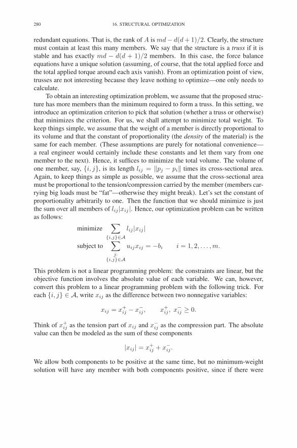
280 16. STRUCTURAL OPTIMIZATION
redundant equations. That is, the rank of A is md− d(d + 1)/2. Clearly, the structure
must contain at least this many members. We say that the structure is a truss if it is
stable and has exactly md − d(d + 1)/2 members. In this case, the force balance
equations have a unique solution (assuming, of course, that the total applied force and
the total applied torque around each axis vanish). From an optimization point of view,
trusses are not interesting because they leave nothing to optimize—one only needs to
calculate.
To obtain an interesting optimization problem, we assume that the proposed struc-
ture has more members than the minimum required to form a truss. In this setting, we
introduce an optimization criterion to pick that solution (whether a truss or otherwise)
that minimizes the criterion. For us, we shall attempt to minimize total weight. To
keep things simple, we assume that the weight of a member is directly proportional to
its volume and that the constant of proportionality (the density of the material) is the
same for each member. (These assumptions are purely for notational convenience—
a real engineer would certainly include these constants and let them vary from one
member to the next). Hence, it suffices to minimize the total volume. The volume of
one member, say, {i, j}, is its length lij = ‖pj − pi‖ times its cross-sectional area.
Again, to keep things as simple as possible, we assume that the cross-sectional area
must be proportional to the tension/compression carried by the member (members car-
rying big loads must be “fat”—otherwise they might break). Let’s set the constant of
proportionality arbitrarily to one. Then the function that we should minimize is just
the sum over all members of lij |xij |. Hence, our optimization problem can be written
as follows:
minimize∑
{i,j}∈Alij |xij |
subject to∑
j:{i,j}∈A
uijxij = −bi i = 1, 2, . . . ,m.
This problem is not a linear programming problem: the constraints are linear, but the
objective function involves the absolute value of each variable. We can, however,
convert this problem to a linear programming problem with the following trick. For
each {i, j} ∈ A, write xij as the difference between two nonnegative variables:
xij = x+ij − x−
ij , x+ij , x−
ij ≥ 0.
Think of x+ij as the tension part of xij and x−
ij as the compression part. The absolute
value can then be modeled as the sum of these components
|xij | = x+ij + x−
ij .
We allow both components to be positive at the same time, but no minimum-weight
solution will have any member with both components positive, since if there were

6. ANCHORS AWAY 281
such a member, the tension component and the compression component could be de-
creased simultaneously at the same rate without changing the force balance equations
but reducing the weight. This reduction contradicts the minimum-weight assumption.
We can now state the linear programming formulation of the minimum weight
structural design problem as follows:
minimize∑
{i,j}∈A(lijx
+ij + lijx
−ij)
subject to∑
j:{i,j}∈A
(uijx+ij − uijx
−ij) = −bi i = 1, 2, . . . , m
x+ij , x−
ij ≥ 0 {i, j} ∈ A.
In terms of the incidence matrix, each column must now be written down twice, once
as before and once as the negative of before.
6. Anchors Away
So far we have considered structures that are free floating in the sense that even
though loads are applied at various joints, we have not assumed that any of the joints
are anchored to a large object such as the Earth. This setup is fine for structures
intended for a rocket or a space station, but for Earth-bound applications it is generally
desired to anchor some joints. It is trivial to modify the formulation we have already
given to cover the situation where some of the joints are anchored. Indeed, the d force
balance equations associated with an anchored joint are simply dropped as constraints,
since the Earth supplies whatever counterbalancing force is needed. Of course, one
can consider dropping only some of the d force balance equations associated with a
particular joint. In this case, the physical interpretation is quite simple. For example,
in two dimensions it simply means that the joint is allowed to roll on a track that is
aligned with one of the coordinate directions but is not allowed to move off the track.
If enough “independent” constraints are dropped (at least three in two dimensions
and at least six in three dimensions), then there are no longer any limitations on the
applied loads—the structure will be sufficiently well anchored so that the Earth will
apply whatever forces are needed to prevent the structure from moving. This is the
most typical scenario under which these problems are solved. It makes setting up the
problem much easier, since one no longer needs to worry about supplying loads that
can’t be balanced.
We end this chapter with one realistic example. Suppose the need exists to design
a bracket to support a hanging load at a fixed distance from a wall. This bracket
will be molded out of plastic, which means that the problem of finding an optimal
design belongs to the realm of continuum mechanics. However, we can get an idea
of the optimal shape by modeling the problem discretely (don’t tell anyone). That is,
we define a lattice of joints as shown in Figure 16.4 and introduce a set of members
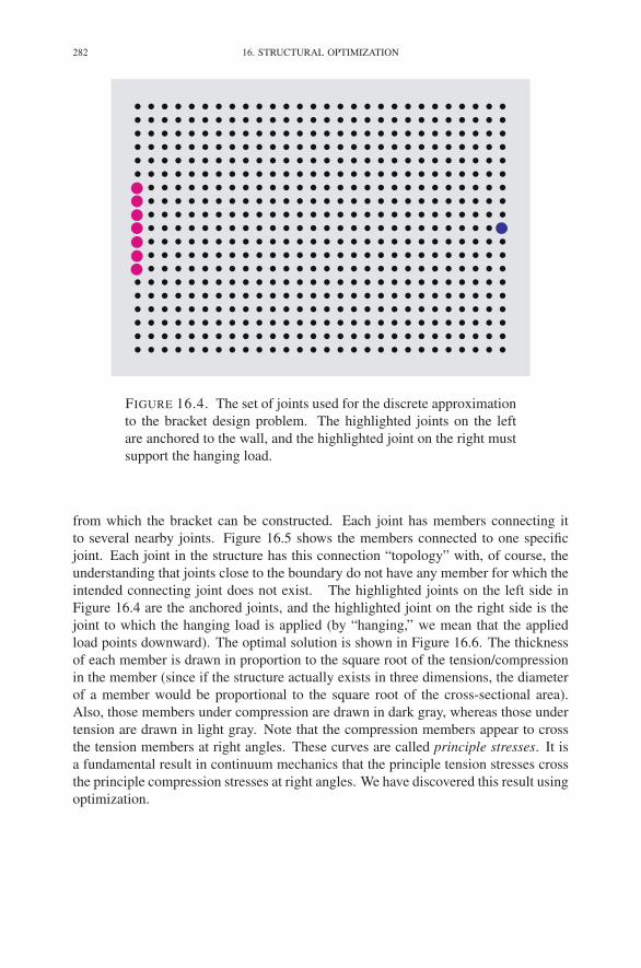
282 16. STRUCTURAL OPTIMIZATION
FIGURE 16.4. The set of joints used for the discrete approximation
to the bracket design problem. The highlighted joints on the left
are anchored to the wall, and the highlighted joint on the right must
support the hanging load.
from which the bracket can be constructed. Each joint has members connecting it
to several nearby joints. Figure 16.5 shows the members connected to one specific
joint. Each joint in the structure has this connection “topology” with, of course, the
understanding that joints close to the boundary do not have any member for which the
intended connecting joint does not exist. The highlighted joints on the left side in
Figure 16.4 are the anchored joints, and the highlighted joint on the right side is the
joint to which the hanging load is applied (by “hanging,” we mean that the applied
load points downward). The optimal solution is shown in Figure 16.6. The thickness
of each member is drawn in proportion to the square root of the tension/compression
in the member (since if the structure actually exists in three dimensions, the diameter
of a member would be proportional to the square root of the cross-sectional area).
Also, those members under compression are drawn in dark gray, whereas those under
tension are drawn in light gray. Note that the compression members appear to cross
the tension members at right angles. These curves are called principle stresses. It is
a fundamental result in continuum mechanics that the principle tension stresses cross
the principle compression stresses at right angles. We have discovered this result using
optimization.
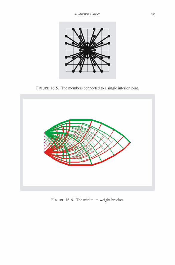
6. ANCHORS AWAY 283
FIGURE 16.5. The members connected to a single interior joint.
FIGURE 16.6. The minimum weight bracket.

284 16. STRUCTURAL OPTIMIZATION
Most nonexperts find the solution to this problem to be quite surprising, since it
covers such a large area. Yet it is indeed optimal. Also, one can see that the continuum
solution should be roughly in the shape of a leaf.
Exercises
16.1 Show that a matrix R is skew symmetric if and only if
ξT Rξ = 0, for every vector ξ.
16.2 Which of the structures shown in Figure 16.7 is stable? (Note: each structure
is shown embedded in a convenient coordinate system.)
16.3 Which of the structures shown in Figure 16.7 is a truss?
16.4 Assuming that the total applied force vanishes, show that total torque is
translation invariant. That is, for any vector ξ ∈ Rd,
∑
i
(R(pi − ξ))T bi =∑
i
(Rpi)T bi.
16.5 In 3-dimensions there are 5 regular (Platonic) solids. They are shown in
Figure 16.8 and have the following number of vertices and edges:
vertices edges
tetrahedron 4 6
cube 8 12
octahedron 6 12
dodecahedron 20 30
icosahedron 12 30
If one were to construct pin-jointed wire-frame models of these solids, which
ones would be stable?
Notes
Structural optimization has its roots in Michell (1904). The first paper in which
truss design was formulated as a linear programming problem is Dorn et al. (1964). A
few general references on the subject include Hemp (1973), Rozvany (1989), Bendsøe
et al. (1994), and Recski (1989).
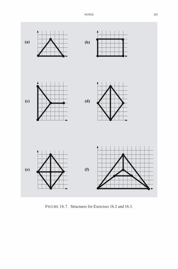
NOTES 285
(a) (b)
(c) (d)
(f)(e)
FIGURE 16.7. Structures for Exercises 16.2 and 16.3.

286 16. STRUCTURAL OPTIMIZATION
FIGURE 16.8. The five regular solids.
CHAPTER 17
The Central Path
In this chapter, we begin our study of an alternative to the simplex method for
solving linear programming problems. The algorithm we are going to introduce is
called a path-following method. It belongs to a class of methods called interior-point
methods. The path-following method seems to be the simplest and most natural of
all the methods in this class, so in this book we focus primarily on it. Before we
can introduce this method, we must define the path that appears in the name of the
method. This path is called the central path and is the subject of this chapter. Before
discussing the central path, we must lay some groundwork by analyzing a nonlinear
problem, called the barrier problem, associated with the linear programming problem
that we wish to solve.
Warning: Nonstandard Notation Ahead
Starting with this chapter, given a lower-case letter denoting a vector quantity, we
shall use the upper-case form of the same letter to denote the diagonal matrix whose
diagonal entries are those of the corresponding vector. For example,
x =
⎡
⎢
⎢
⎢
⎢
⎢
⎣
x1
x2
...
xn
⎤
⎥
⎥
⎥
⎥
⎥
⎦
=⇒ X =
⎡
⎢
⎢
⎢
⎢
⎢
⎣
x1
x2
. . .
xn
⎤
⎥
⎥
⎥
⎥
⎥
⎦
.
This notation is nonstandard in mathematics at large, but has achieved a certain amount
of acceptance in the interior-point-methods community.
1. The Barrier Problem
In this chapter, we consider the linear programming problem expressed, as usual,
with inequality constraints and nonnegative variables:
maximize cT x
subject to Ax≤ b
x≥ 0.
289
290 17. THE CENTRAL PATH
The corresponding dual problem is
minimize bT y
subject to AT y ≥ c
y ≥ 0.
As usual, we add slack variables to convert both problems to equality form:
(17.1)
maximize cT x
subject to Ax + w = b
x, w ≥ 0
and
minimize bT y
subject to AT y − z = c
y, z ≥ 0.
Given a constrained maximization problem where some of the constraints are
inequalities (such as our primal linear programming problem), one can consider re-
placing any inequality constraint with an extra term in the objective function. For
example, in (17.1) we could remove the constraint that a specific variable, say, xj , is
nonnegative by adding to the objective function a term that is negative infinity when xj
is negative and is zero otherwise. This reformulation doesn’t seem to be particularly
helpful, since this new objective function has an abrupt discontinuity that, for exam-
ple, prevents us from using calculus to study it. However, suppose we replace this
discontinuous function with another function that is negative infinity when xj is nega-
tive but is finite for xj positive and approaches negative infinity as xj approaches zero.
In some sense this smooths out the discontinuity and perhaps improves our ability to
apply calculus to its study. The simplest such function is the logarithm. Hence, for
each variable, we introduce a new term in the objective function that is just a constant
times the logarithm of the variable:
(17.2)maximize cT x + μ
∑
j log xj + μ∑
i log wi
subject to Ax + w = b.
This problem, while not equivalent to our original problem, seems not too different
either. In fact, as the parameter μ, which we assume to be positive, gets small, it
appears that (17.2) becomes a better and better stand-in for (17.1). Problem (17.2)
is called the barrier problem associated with (17.1). Note that it is not really one
problem, but rather a whole family of problems indexed by the parameter μ. Each of
these problems is a nonlinear programming problem because the objective function
is nonlinear. This nonlinear objective function is called a barrier function or, more
specifically, a logarithmic barrier function.
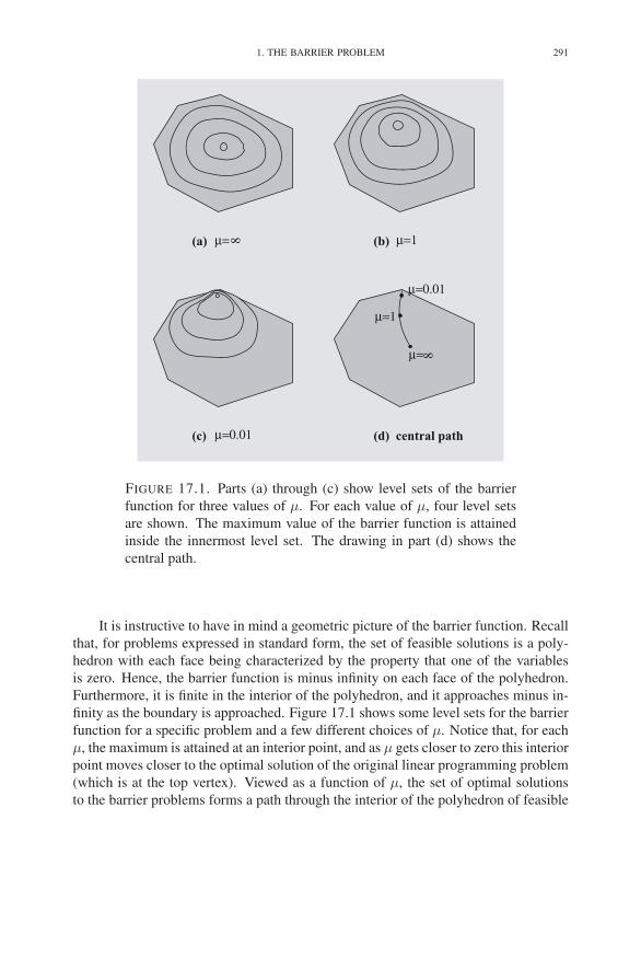
1. THE BARRIER PROBLEM 291
µ= 8
µ=1
µ=0.01
(a) µ= 8 (b) µ=1
(c) µ=0.01 (d) central path
FIGURE 17.1. Parts (a) through (c) show level sets of the barrier
function for three values of μ. For each value of μ, four level sets
are shown. The maximum value of the barrier function is attained
inside the innermost level set. The drawing in part (d) shows the
central path.
It is instructive to have in mind a geometric picture of the barrier function. Recall
that, for problems expressed in standard form, the set of feasible solutions is a poly-
hedron with each face being characterized by the property that one of the variables
is zero. Hence, the barrier function is minus infinity on each face of the polyhedron.
Furthermore, it is finite in the interior of the polyhedron, and it approaches minus in-
finity as the boundary is approached. Figure 17.1 shows some level sets for the barrier
function for a specific problem and a few different choices of μ. Notice that, for each
μ, the maximum is attained at an interior point, and as μ gets closer to zero this interior
point moves closer to the optimal solution of the original linear programming problem
(which is at the top vertex). Viewed as a function of μ, the set of optimal solutions
to the barrier problems forms a path through the interior of the polyhedron of feasible

292 17. THE CENTRAL PATH
g=0x*
∆
f
FIGURE 17.2. The concentric rings illustrate a few level sets of f .
Clearly, at the optimal solution, x∗, the gradient must be perpendic-
ular to the feasible set.
solutions. This path is called the central path. Our aim is to study this central path. To
this end, we need to develop some machinery, referred to as Lagrange multipliers.
2. Lagrange Multipliers
We wish to discuss briefly the general problem of maximizing a function subject
to one or more equality constraints. Here, the functions are permitted to be nonlinear,
but are assumed to be smooth, say, twice differentiable.
For the moment, suppose that there is a single constraint equation so that the
problem can be formally stated as
maximize f(x)
subject to g(x) = 0.
In this case, the geometry behind the problem is compelling (see Figure 17.2). The
gradient of f , denoted ∇f , is a vector that points in the direction of most rapid increase
of f . For unconstrained optimization, we would simply set this vector equal to zero
to determine the so-called critical points of f , and the maximum, if it exists, would
have to be included in this set. However, given the constraint, g(x) = 0, it is no longer
correct to look at points where the gradient vanishes. Instead, the gradient must be
orthogonal to the set of feasible solutions {x : g(x) = 0}. Of course, at each point xin the feasible set, ∇g(x), is a vector that is orthogonal to the feasible set at this point
x. Hence, our new requirement for a point x∗ to be a critical point is that it is feasible
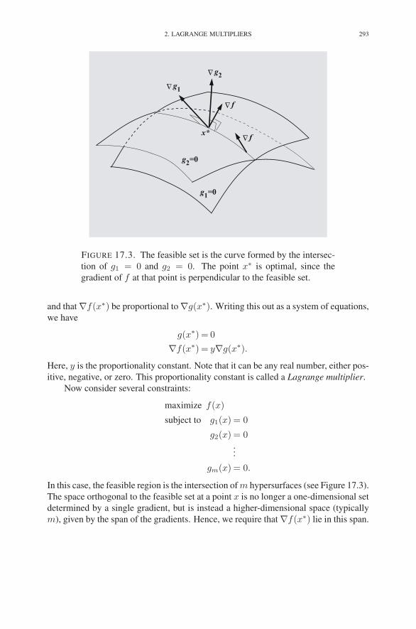
2. LAGRANGE MULTIPLIERS 293
g1=0
x*
g2=0
∆
g2
∆
g1
∆
f
∆
f
FIGURE 17.3. The feasible set is the curve formed by the intersec-
tion of g1 = 0 and g2 = 0. The point x∗ is optimal, since the
gradient of f at that point is perpendicular to the feasible set.
and that ∇f(x∗) be proportional to ∇g(x∗). Writing this out as a system of equations,
we have
g(x∗) = 0
∇f(x∗) = y∇g(x∗).
Here, y is the proportionality constant. Note that it can be any real number, either pos-
itive, negative, or zero. This proportionality constant is called a Lagrange multiplier.
Now consider several constraints:
maximize f(x)
subject to g1(x) = 0
g2(x) = 0...
gm(x) = 0.
In this case, the feasible region is the intersection of m hypersurfaces (see Figure 17.3).
The space orthogonal to the feasible set at a point x is no longer a one-dimensional set
determined by a single gradient, but is instead a higher-dimensional space (typically
m), given by the span of the gradients. Hence, we require that ∇f(x∗) lie in this span.

294 17. THE CENTRAL PATH
This yields the following set of equations for a critical point:
g(x∗) = 0
∇f(x∗) =m∑
i=1
yi∇g(x∗).(17.3)
The derivation of these equations has been entirely geometric, but there is also a
simple algebraic formalism that yields the same equations. The idea is to introduce
the so-called Lagrangian function
L(x, y) = f(x) −∑
i
yigi(x)
and to look for its critical points over both x and y. Since this is now an unconstrained
optimization problem, the critical points are determined by simply setting all the first
derivatives to zero:
∂L
∂xj=
∂f
∂xj−
∑
i
yi∂gi
∂xj= 0, j = 1, 2, . . . , n,
∂L
∂yi= −gi = 0, i = 1, 2, . . . ,m.
Writing these equations in vector notation, we see that they are exactly the same as
those derived using the geometric approach. These equations are usually referred to
as the first-order optimality conditions.
Determining whether a solution to the first-order optimality conditions is indeed a
global maximum as desired can be difficult. However, if the constraints are all linear,
the first step (which is often sufficient) is to look at the matrix of second derivatives:
Hf(x) =
[
∂2f
∂xi∂xj
]
.
This matrix is called the Hessian of f at x. We have
THEOREM 17.1. If the constraints are linear, a critical point x∗ is a local maxi-
mum if
(17.4) ξT Hf(x∗)ξ < 0
for each ξ �= 0 satisfying
(17.5) ξT∇gi(x∗) = 0, i = 1, 2, . . . ,m.
PROOF. We start with the two-term Taylor series expansion of f about x∗:
f(x∗ + ξ) = f(x∗) + ∇f(x∗)T ξ +1
2ξT Hf(x∗)ξ + o(‖ξ‖2).

3. LAGRANGE MULTIPLIERS APPLIED TO THE BARRIER PROBLEM 295
The vector ξ represents a displacement from the current point x∗. The only displace-
ments that are relevant are those that lie in the feasible set. Hence, let ξ be a direction
vector satisfying (17.5). From (17.3) and (17.5), we see that ∇f(x∗)T ξ = 0, and so
f(x∗ + ξ) = f(x∗) +1
2ξT Hf(x∗)ξ + o(‖ξ‖2).
Employing (17.4) finishes the proof. �
It is worth remarking that if (17.4) is satisfied not just at x∗ but at all x, then x∗ is
a unique global maximum.
In the next section, we shall use Lagrange multipliers to study the central path
defined by the barrier problem.
3. Lagrange Multipliers Applied to the Barrier Problem
In this section, we shall use the machinery of Lagrange multipliers to study the
solution to the barrier problem. In particular, we will show that (subject to some mild
assumptions) for each value of the barrier parameter μ, there is a unique solution to
the barrier problem. We will also show that as μ tends to zero, the solution to the
barrier problem tends to the solution to the original linear programming problem. In
the course of our study, we will stumble naturally upon the central path for the dual
problem. Taken together, the equations defining the primal and the dual central paths
play an important role, and so we will introduce the notion of a primal–dual central
path.
We begin by recalling the barrier problem:
maximize cT x + μ∑
j log xj + μ∑
i log wi
subject to Ax + w = b.
This is an equality-constrained optimization problem, and so it is a problem to which
we can apply the Lagrange multiplier tools developed in the previous section. The
Lagrangian for this problem is
L(x,w, y) = cT x + μ∑
j
log xj + μ∑
i
log wi + yT (b − Ax − w).
Taking derivatives with respect to each variable and setting them to zero, we get the
first-order optimality conditions:
∂L
∂xj= cj + μ
1
xj−
∑
i
yiaij = 0, j = 1, 2, . . . , n,
∂L
∂wi= μ
1
wi− yi = 0, i = 1, 2, . . . ,m.
∂L
∂yi= bi −
∑
j
aijxj − wi = 0, i = 1, 2, . . . ,m.
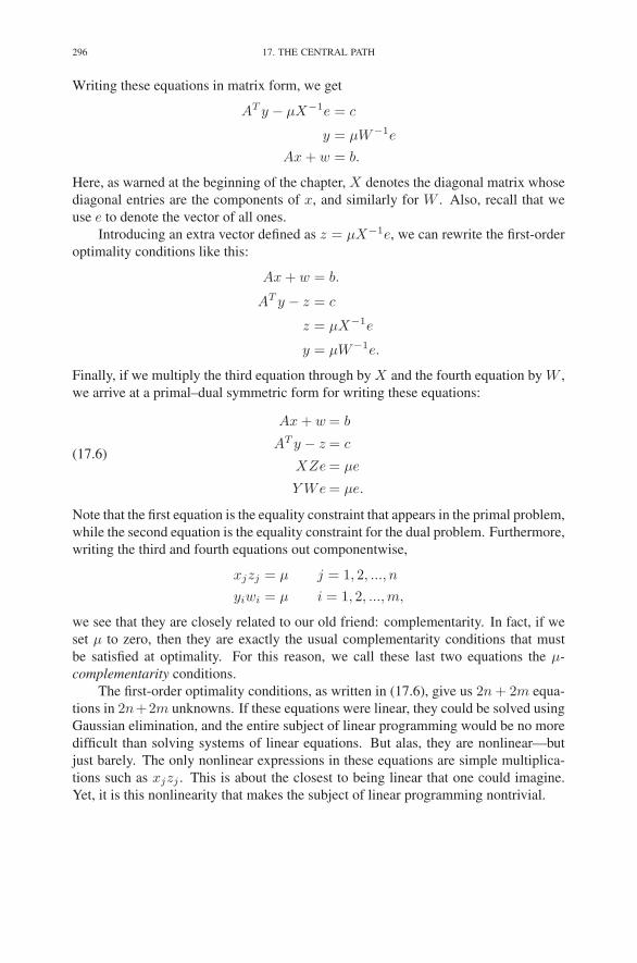
296 17. THE CENTRAL PATH
Writing these equations in matrix form, we get
AT y − μX−1e = c
y = μW−1e
Ax + w = b.
Here, as warned at the beginning of the chapter, X denotes the diagonal matrix whose
diagonal entries are the components of x, and similarly for W . Also, recall that we
use e to denote the vector of all ones.
Introducing an extra vector defined as z = μX−1e, we can rewrite the first-order
optimality conditions like this:
Ax + w = b.
AT y − z = c
z = μX−1e
y = μW−1e.
Finally, if we multiply the third equation through by X and the fourth equation by W ,
we arrive at a primal–dual symmetric form for writing these equations:
(17.6)
Ax + w = b
AT y − z = c
XZe = μe
Y We = μe.
Note that the first equation is the equality constraint that appears in the primal problem,
while the second equation is the equality constraint for the dual problem. Furthermore,
writing the third and fourth equations out componentwise,
xjzj = μ j = 1, 2, ..., n
yiwi = μ i = 1, 2, ...,m,
we see that they are closely related to our old friend: complementarity. In fact, if we
set μ to zero, then they are exactly the usual complementarity conditions that must
be satisfied at optimality. For this reason, we call these last two equations the μ-
complementarity conditions.
The first-order optimality conditions, as written in (17.6), give us 2n + 2m equa-
tions in 2n+2m unknowns. If these equations were linear, they could be solved using
Gaussian elimination, and the entire subject of linear programming would be no more
difficult than solving systems of linear equations. But alas, they are nonlinear—but
just barely. The only nonlinear expressions in these equations are simple multiplica-
tions such as xjzj . This is about the closest to being linear that one could imagine.
Yet, it is this nonlinearity that makes the subject of linear programming nontrivial.

5. EXISTENCE 297
We must ask both whether a solution to (17.6) exists and if so is it unique. We
address these questions in reverse order.
4. Second-Order Information
To show that the solution, if it is exists, must be unique, we use second-order
information on the barrier function:
(17.7) f(x,w) = cT x + μ∑
j
log xj + μ∑
i
log wi.
The first derivatives are
∂f
∂xj= cj +
μ
xj, j = 1, 2, . . . , n,
∂f
∂wi=
μ
wi, i = 1, 2, . . . ,m,
and the pure second derivatives are
∂2f
∂x2j
= − μ
x2j
, j = 1, 2, . . . , n,
∂2f
∂w2i
= − μ
w2i
, i = 1, 2, . . . ,m.
All the mixed second derivatives vanish. Therefore, the Hessian is a diagonal matrix
with strictly negative entries. Hence, by Theorem 17.1, there can be at most one
critical point and, if it exists, it is a global maximum.
5. Existence
So, does a solution to the barrier problem always exist? It might not. Consider,
for example, the following trivial optimization problem on the nonnegative half-line:
maximize 0
subject to x ≥ 0.
For this problem, the barrier function is
f(x) = μ log x,
which doesn’t have a maximum (or, less precisely, the maximum is infinity which
is attained at x = ∞). However, such examples are rare. For example, consider
modifying the objective function in this example to make x = 0 the unique optimal
solution:
maximize −x
subject to x ≥ 0.
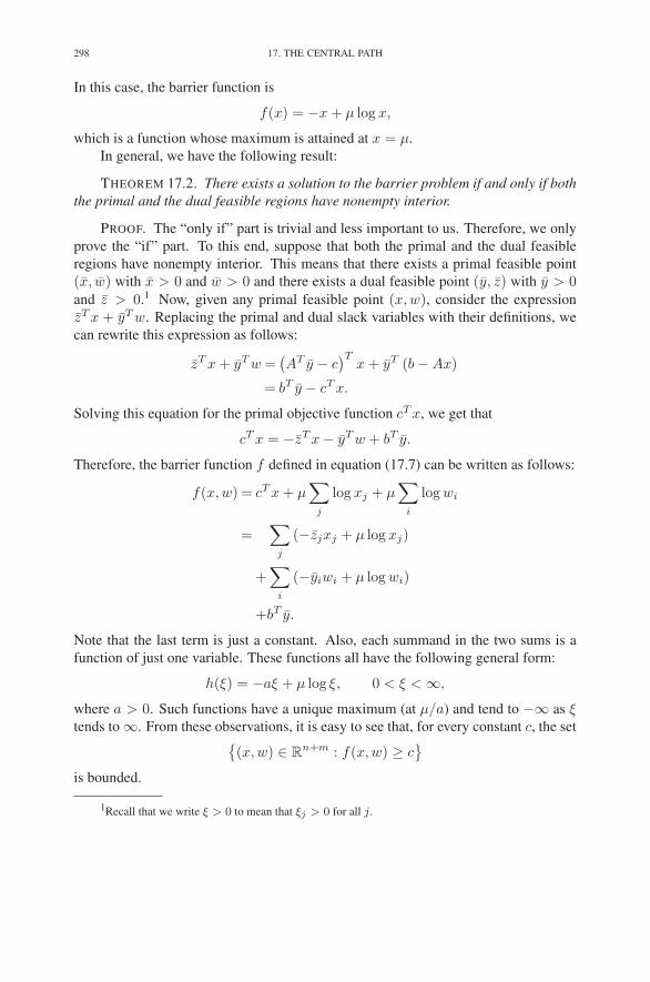
298 17. THE CENTRAL PATH
In this case, the barrier function is
f(x) = −x + μ log x,
which is a function whose maximum is attained at x = μ.
In general, we have the following result:
THEOREM 17.2. There exists a solution to the barrier problem if and only if both
the primal and the dual feasible regions have nonempty interior.
PROOF. The “only if” part is trivial and less important to us. Therefore, we only
prove the “if” part. To this end, suppose that both the primal and the dual feasible
regions have nonempty interior. This means that there exists a primal feasible point
(x, w) with x > 0 and w > 0 and there exists a dual feasible point (y, z) with y > 0and z > 0.1 Now, given any primal feasible point (x,w), consider the expression
zT x + yT w. Replacing the primal and dual slack variables with their definitions, we
can rewrite this expression as follows:
zT x + yT w =(
AT y − c)T
x + yT (b − Ax)
= bT y − cT x.
Solving this equation for the primal objective function cT x, we get that
cT x = −zT x − yT w + bT y.
Therefore, the barrier function f defined in equation (17.7) can be written as follows:
f(x,w) = cT x + μ∑
j
log xj + μ∑
i
log wi
=∑
j
(−zjxj + μ log xj)
+∑
i
(−yiwi + μ log wi)
+bT y.
Note that the last term is just a constant. Also, each summand in the two sums is a
function of just one variable. These functions all have the following general form:
h(ξ) = −aξ + μ log ξ, 0 < ξ < ∞,
where a > 0. Such functions have a unique maximum (at μ/a) and tend to −∞ as ξtends to ∞. From these observations, it is easy to see that, for every constant c, the set
{
(x,w) ∈ Rn+m : f(x,w) ≥ c
}
is bounded.
1Recall that we write ξ > 0 to mean that ξj > 0 for all j.

EXERCISES 299
Put
f = f(x, w)
and let
P = {(x,w) : Ax + w = b, x ≥ 0, w ≥ 0, f(x,w) ≥ f}.Clearly, P is nonempty, since it contains (x, w). From the discussion above, we see
that P is a bounded set.
This set is also closed. To see this, note that it is the intersection of three sets,
{(x,w) : Ax + w = b} ∩ {(x,w) : x ≥ 0, w ≥ 0} ∩ {(x,w) : f(x,w) ≥ f}.The first two of these sets are obviously closed. The third set is closed because it is
the inverse image of a closed set, [f ,∞], under a continuous mapping f . Finally, the
intersection of three closed sets is closed.
In Euclidean spaces, a closed bounded set is called compact. A well-known theo-
rem from real analysis about compact sets is that a continuous function on a nonempty
compact set attains its maximum. This means that there exists a point in the compact
set at which the function hits its maximum. Applying this theorem to f on P , we see
that f does indeed attain its maximum on P , and this implies it attains its maximum
on all of {(x,w) : x > 0, w > 0}, since P was by definition that part of this domain
on which f takes large values (bigger than f , anyway). This completes the proof. �
We summarize our main result in the following corollary:
COROLLARY 17.3. If a primal feasible set (or, for that matter, its dual) has a
nonempty interior and is bounded, then for each μ > 0 there exists a unique solution
(xμ, wμ, yμ, zμ)
to (17.6).
PROOF. Follows immediately from the previous theorem and Exercise 10.7. �
The path {(xμ, wμ, yμ, zμ) : μ > 0} is called the primal–dual central path. It
plays a fundamental role in interior-point methods for linear programming. In the next
chapter, we define the simplest interior-point method. It is an iterative procedure that
at each iteration attempts to move toward a point on the central path that is closer to
optimality than the current point.
Exercises
17.1 Compute and graph the central trajectory for the following problem:
maximize −x1 + x2
subject to x2 ≤ 1
−x1 ≤−1
x1, x2 ≥ 0.
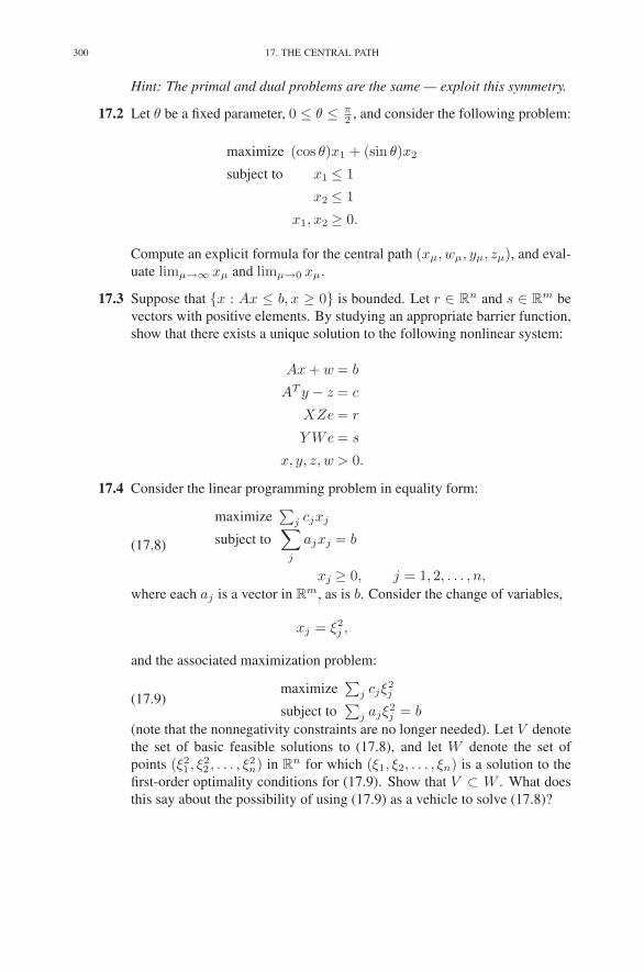
300 17. THE CENTRAL PATH
Hint: The primal and dual problems are the same — exploit this symmetry.
17.2 Let θ be a fixed parameter, 0 ≤ θ ≤ π2 , and consider the following problem:
maximize (cos θ)x1 + (sin θ)x2
subject to x1 ≤ 1
x2 ≤ 1
x1, x2 ≥ 0.
Compute an explicit formula for the central path (xμ, wμ, yμ, zμ), and eval-
uate limμ→∞ xμ and limμ→0 xμ.
17.3 Suppose that {x : Ax ≤ b, x ≥ 0} is bounded. Let r ∈ Rn and s ∈ R
m be
vectors with positive elements. By studying an appropriate barrier function,
show that there exists a unique solution to the following nonlinear system:
Ax + w = b
AT y − z = c
XZe = r
Y We = s
x, y, z, w > 0.
17.4 Consider the linear programming problem in equality form:
(17.8)
maximize∑
j cjxj
subject to∑
j
ajxj = b
xj ≥ 0, j = 1, 2, . . . , n,
where each aj is a vector in Rm, as is b. Consider the change of variables,
xj = ξ2j ,
and the associated maximization problem:
(17.9)maximize
∑
j cjξ2j
subject to∑
j ajξ2j = b
(note that the nonnegativity constraints are no longer needed). Let V denote
the set of basic feasible solutions to (17.8), and let W denote the set of
points (ξ21 , ξ2
2 , . . . , ξ2n) in R
n for which (ξ1, ξ2, . . . , ξn) is a solution to the
first-order optimality conditions for (17.9). Show that V ⊂ W . What does
this say about the possibility of using (17.9) as a vehicle to solve (17.8)?

NOTES 301
Notes
Research into interior-point methods has its roots in the work of Fiacco & Mc-
Cormick (1968). Interest in these methods exploded after the appearance of the sem-
inal paper Karmarkar (1984). Karmarkar’s paper uses clever ideas from projective
geometry. It doesn’t mention anything about central paths, which have become fun-
damental to the theory of interior-point methods. The discovery that Karmarkar’s
algorithm has connections with the primal–dual central path introduced in this chapter
can be traced to Megiddo (1989). The notion of central points can be traced to pre-
Karmarkar times with the work of Huard (1967). D.A. Bayer and J.C. Lagarias, in a
pair of papers (Bayer & Lagarias 1989a,b), give an in-depth study of the central path.
Deriving optimality conditions and giving conditions under which they are nec-
essary and sufficient to guarantee optimality is one of the main goals of nonlinear
programming. Standard texts on this subject include the books by Luenberger (1984),
Bertsekas (1995), and Nash & Sofer (1996).

CHAPTER 18
A Path-Following Method
In this chapter, we define an interior-point method for linear programming that
is called a path-following method. Recall that for the simplex method we required
a two-phase solution procedure. The path-following method is a one-phase method.
This means that the method can begin from a point that is neither primal nor dual
feasible and it will proceed from there directly to the optimal solution. Hence, we
start with an arbitrary choice of strictly positive values for all the primal and dual
variables, i.e., (x,w, y, z) > 0, and then iteratively update these values as follows:
(1) Estimate an appropriate value for μ (i.e., smaller than the “current” value
but not too small).
(2) Compute step directions (∆x,∆w,∆y,∆z) pointing approximately at the
point (xμ, wμ, yμ, zμ) on the central path.
(3) Compute a step length parameter θ such that the new point
x = x + θ∆x, y = y + θ∆y,
w = w + θ∆w, z = z + θ∆z
continues to have strictly positive components.
(4) Replace (x,w, y, z) with the new solution (x, w, y, z).
To fully define the path-following method, it suffices to make each of these four steps
precise. Since the second step is in some sense the most fundamental, we start by
describing that one after which we turn our attention to the others.
1. Computing Step Directions
Our aim is to find (∆x,∆w,∆y,∆z) such that the new point (x + ∆x,w +∆w, y + ∆y, z + ∆z) lies approximately on the primal–dual central path at the point
(xμ, wμ, yμ, zμ). Recalling the defining equations for this point on the central path,
Ax + w = b
AT y − z = c
XZe = μe
Y We = μe,
303
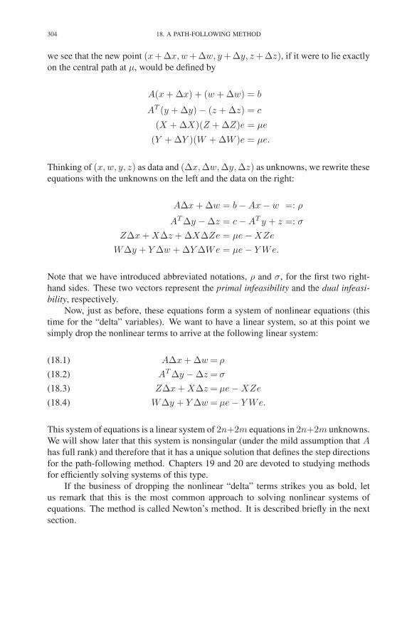
304 18. A PATH-FOLLOWING METHOD
we see that the new point (x+∆x,w +∆w, y +∆y, z +∆z), if it were to lie exactly
on the central path at μ, would be defined by
A(x + ∆x) + (w + ∆w) = b
AT (y + ∆y) − (z + ∆z) = c
(X + ∆X)(Z + ∆Z)e = μe
(Y + ∆Y )(W + ∆W )e = μe.
Thinking of (x,w, y, z) as data and (∆x,∆w,∆y,∆z) as unknowns, we rewrite these
equations with the unknowns on the left and the data on the right:
A∆x + ∆w = b − Ax − w =: ρ
AT ∆y − ∆z = c − AT y + z =: σ
Z∆x + X∆z + ∆X∆Ze = μe − XZe
W∆y + Y ∆w + ∆Y ∆We = μe − Y We.
Note that we have introduced abbreviated notations, ρ and σ, for the first two right-
hand sides. These two vectors represent the primal infeasibility and the dual infeasi-
bility, respectively.
Now, just as before, these equations form a system of nonlinear equations (this
time for the “delta” variables). We want to have a linear system, so at this point we
simply drop the nonlinear terms to arrive at the following linear system:
A∆x + ∆w = ρ(18.1)
AT ∆y − ∆z = σ(18.2)
Z∆x + X∆z = μe − XZe(18.3)
W∆y + Y ∆w = μe − Y We.(18.4)
This system of equations is a linear system of 2n+2m equations in 2n+2m unknowns.
We will show later that this system is nonsingular (under the mild assumption that Ahas full rank) and therefore that it has a unique solution that defines the step directions
for the path-following method. Chapters 19 and 20 are devoted to studying methods
for efficiently solving systems of this type.
If the business of dropping the nonlinear “delta” terms strikes you as bold, let
us remark that this is the most common approach to solving nonlinear systems of
equations. The method is called Newton’s method. It is described briefly in the next
section.
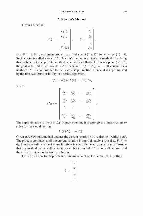
2. NEWTON’S METHOD 305
2. Newton’s Method
Given a function
F (ξ) =
⎡
⎢
⎢
⎢
⎢
⎢
⎣
F1(ξ)
F2(ξ)...
FN (ξ)
⎤
⎥
⎥
⎥
⎥
⎥
⎦
, ξ =
⎡
⎢
⎢
⎢
⎢
⎢
⎣
ξ1
ξ2
...
ξN
⎤
⎥
⎥
⎥
⎥
⎥
⎦
,
from RN into R
N , a common problem is to find a point ξ∗ ∈ RN for which F (ξ∗) = 0.
Such a point is called a root of F . Newton’s method is an iterative method for solving
this problem. One step of the method is defined as follows. Given any point ξ ∈ RN ,
the goal is to find a step direction ∆ξ for which F (ξ + ∆ξ) = 0. Of course, for a
nonlinear F it is not possible to find such a step direction. Hence, it is approximated
by the first two terms of its Taylor’s series expansion,
F (ξ + ∆ξ) ≈ F (ξ) + F ′(ξ)∆ξ,
where
F ′(ξ) =
⎡
⎢
⎢
⎢
⎢
⎢
⎢
⎢
⎢
⎢
⎢
⎣
∂F1
∂ξ1
∂F1
∂ξ2· · · ∂F1
∂ξN
∂F2
∂ξ1
∂F2
∂ξ2· · · ∂F2
∂ξN
......
...
∂FN
∂ξ1
∂FN
∂ξ2· · · ∂FN
∂ξN
⎤
⎥
⎥
⎥
⎥
⎥
⎥
⎥
⎥
⎥
⎥
⎦
.
The approximation is linear in ∆ξ. Hence, equating it to zero gives a linear system to
solve for the step direction:
F ′(ξ)∆ξ = −F (ξ).
Given ∆ξ, Newton’s method updates the current solution ξ by replacing it with ξ+∆ξ.
The process continues until the current solution is approximately a root (i.e., F (ξ) ≈0). Simple one-dimensional examples given in every elementary calculus text illustrate
that this method works well, when it works, but it can fail if F is not well behaved and
the initial point is too far from a solution.
Let’s return now to the problem of finding a point on the central path. Letting
ξ =
⎡
⎢
⎢
⎢
⎢
⎣
x
w
y
z
⎤
⎥
⎥
⎥
⎥
⎦
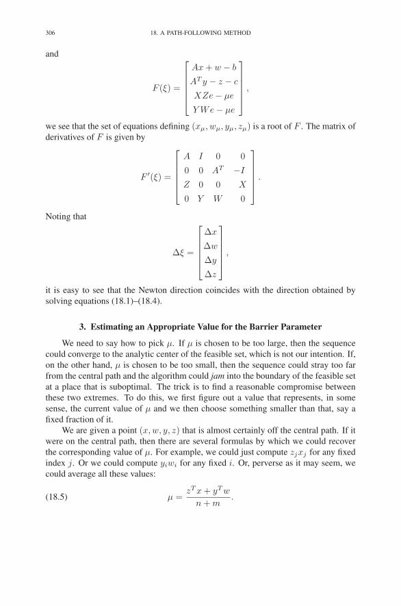
306 18. A PATH-FOLLOWING METHOD
and
F (ξ) =
⎡
⎢
⎢
⎢
⎢
⎣
Ax + w − b
AT y − z − c
XZe − μe
Y We − μe
⎤
⎥
⎥
⎥
⎥
⎦
,
we see that the set of equations defining (xμ, wμ, yμ, zμ) is a root of F . The matrix of
derivatives of F is given by
F ′(ξ) =
⎡
⎢
⎢
⎢
⎢
⎣
A I 0 0
0 0 AT −I
Z 0 0 X
0 Y W 0
⎤
⎥
⎥
⎥
⎥
⎦
.
Noting that
∆ξ =
⎡
⎢
⎢
⎢
⎢
⎣
∆x
∆w
∆y
∆z
⎤
⎥
⎥
⎥
⎥
⎦
,
it is easy to see that the Newton direction coincides with the direction obtained by
solving equations (18.1)–(18.4).
3. Estimating an Appropriate Value for the Barrier Parameter
We need to say how to pick μ. If μ is chosen to be too large, then the sequence
could converge to the analytic center of the feasible set, which is not our intention. If,
on the other hand, μ is chosen to be too small, then the sequence could stray too far
from the central path and the algorithm could jam into the boundary of the feasible set
at a place that is suboptimal. The trick is to find a reasonable compromise between
these two extremes. To do this, we first figure out a value that represents, in some
sense, the current value of μ and we then choose something smaller than that, say a
fixed fraction of it.
We are given a point (x,w, y, z) that is almost certainly off the central path. If it
were on the central path, then there are several formulas by which we could recover
the corresponding value of μ. For example, we could just compute zjxj for any fixed
index j. Or we could compute yiwi for any fixed i. Or, perverse as it may seem, we
could average all these values:
(18.5) μ =zT x + yT w
n + m.
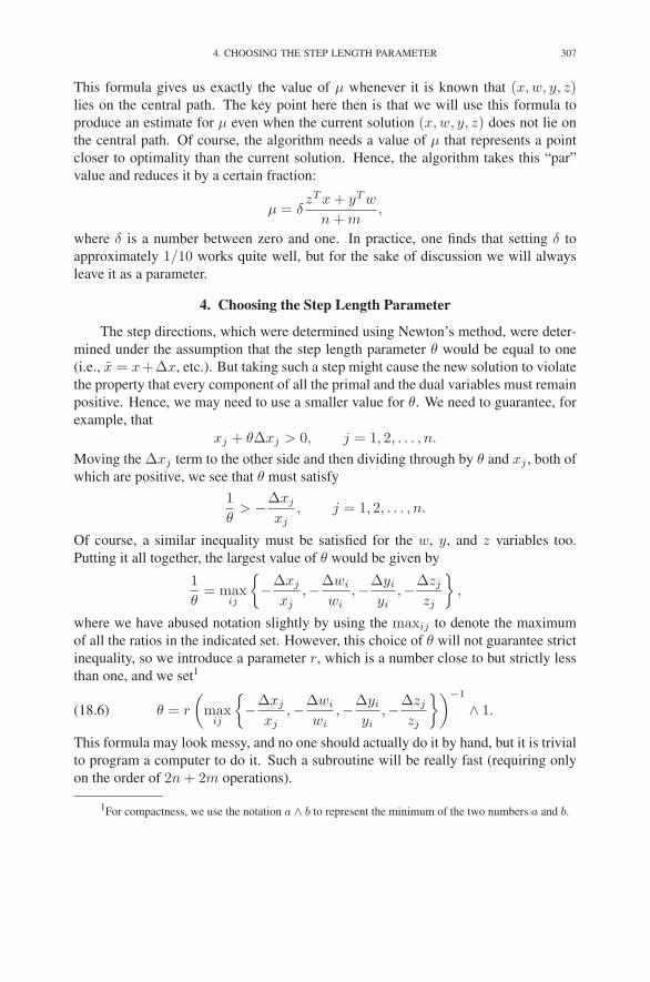
4. CHOOSING THE STEP LENGTH PARAMETER 307
This formula gives us exactly the value of μ whenever it is known that (x,w, y, z)lies on the central path. The key point here then is that we will use this formula to
produce an estimate for μ even when the current solution (x,w, y, z) does not lie on
the central path. Of course, the algorithm needs a value of μ that represents a point
closer to optimality than the current solution. Hence, the algorithm takes this “par”
value and reduces it by a certain fraction:
μ = δzT x + yT w
n + m,
where δ is a number between zero and one. In practice, one finds that setting δ to
approximately 1/10 works quite well, but for the sake of discussion we will always
leave it as a parameter.
4. Choosing the Step Length Parameter
The step directions, which were determined using Newton’s method, were deter-
mined under the assumption that the step length parameter θ would be equal to one
(i.e., x = x+∆x, etc.). But taking such a step might cause the new solution to violate
the property that every component of all the primal and the dual variables must remain
positive. Hence, we may need to use a smaller value for θ. We need to guarantee, for
example, that
xj + θ∆xj > 0, j = 1, 2, . . . , n.
Moving the ∆xj term to the other side and then dividing through by θ and xj , both of
which are positive, we see that θ must satisfy
1
θ> −∆xj
xj, j = 1, 2, . . . , n.
Of course, a similar inequality must be satisfied for the w, y, and z variables too.
Putting it all together, the largest value of θ would be given by
1
θ= max
ij
{
−∆xj
xj,−∆wi
wi,−∆yi
yi,−∆zj
zj
}
,
where we have abused notation slightly by using the maxij to denote the maximum
of all the ratios in the indicated set. However, this choice of θ will not guarantee strict
inequality, so we introduce a parameter r, which is a number close to but strictly less
than one, and we set1
(18.6) θ = r
(
maxij
{
−∆xj
xj,−∆wi
wi,−∆yi
yi,−∆zj
zj
})−1
∧ 1.
This formula may look messy, and no one should actually do it by hand, but it is trivial
to program a computer to do it. Such a subroutine will be really fast (requiring only
on the order of 2n + 2m operations).
1For compactness, we use the notation a ∧ b to represent the minimum of the two numbers a and b.
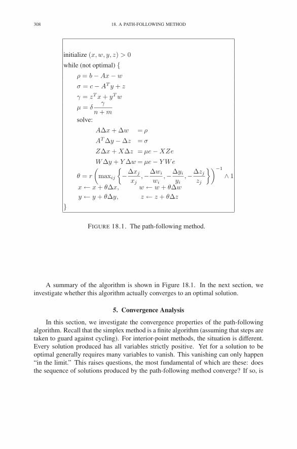
308 18. A PATH-FOLLOWING METHOD
initialize (x,w, y, z) > 0
while (not optimal) {ρ = b − Ax − w
σ = c − AT y + z
γ = zT x + yT w
μ = δγ
n + msolve:
A∆x + ∆w = ρ
AT ∆y − ∆z = σ
Z∆x + X∆z = μe − XZe
W∆y + Y ∆w = μe − Y We
θ = r
(
maxij
{
−∆xj
xj,−∆wi
wi,−∆yi
yi,−∆zj
zj
})−1
∧ 1
x ← x + θ∆x, w ← w + θ∆w
y ← y + θ∆y, z ← z + θ∆z
}
FIGURE 18.1. The path-following method.
A summary of the algorithm is shown in Figure 18.1. In the next section, we
investigate whether this algorithm actually converges to an optimal solution.
5. Convergence Analysis
In this section, we investigate the convergence properties of the path-following
algorithm. Recall that the simplex method is a finite algorithm (assuming that steps are
taken to guard against cycling). For interior-point methods, the situation is different.
Every solution produced has all variables strictly positive. Yet for a solution to be
optimal generally requires many variables to vanish. This vanishing can only happen
“in the limit.” This raises questions, the most fundamental of which are these: does
the sequence of solutions produced by the path-following method converge? If so, is

5. CONVERGENCE ANALYSIS 309
the limit optimal? How fast is the convergence? In particular, if we set “optimality
tolerances,” how many iterations will it take to achieve these tolerances? We will
address these questions in this section.
In this section, we will need to measure the size of various vectors. There are
many choices. For example, for each 1 ≤ p < ∞, we can define the so-called p-norm
of a vector x as
‖x‖p =
⎛
⎝
∑
j
|xj |p⎞
⎠
1p
.
The limit as p tends to infinity is also well defined, and it simplifies to the so-called
sup-norm:
‖x‖∞ = maxj
|xj |.
5.1. Measures of Progress. Recall from duality theory that there are three crite-
ria that must be met in order that a primal–dual solution be optimal:
(1) Primal feasibility,
(2) Dual feasibility, and
(3) Complementarity.
For each of these criteria, we introduce a measure of the extent to which they fail to
be met.
For the primal feasibility criterion, we use the 1-norm of the primal infeasibility
vector
ρ = b − Ax − w.
For the dual feasibility criterion, we use the 1-norm of the dual infeasibility vector
σ = c − AT y + z.
For complementarity, we use
γ = zT x + yT w.
5.2. Progress in One Iteration. For the analysis in the section, we prefer to
modify the algorithm slightly by having it take shorter steps than specified before.
Indeed, we let
θ = r
(
maxi,j
{∣
∣
∣
∣
∆xj
xj
∣
∣
∣
∣
,
∣
∣
∣
∣
∆wi
wi
∣
∣
∣
∣
,
∣
∣
∣
∣
∆yi
yi
∣
∣
∣
∣
,
∣
∣
∣
∣
∆zj
zj
∣
∣
∣
∣
})−1
∧ 1
=r
max(‖X−1∆x‖∞, . . . , ‖Z−1∆z‖∞)∧ 1.(18.7)
Note that the only change has been to replace the negative ratios with the absolute
value of the same ratios. Since the maximum of the absolute values can be larger than
the maximum of the ratios themselves, this formula produces a smaller value for θ. In
this section, let x, y, etc., denote quantities from one iteration of the algorithm, and
310 18. A PATH-FOLLOWING METHOD
put a tilde on the same letters to denote the same quantity at the next iteration of the
algorithm. Hence,
x = x + θ∆x, y = y + θ∆y,
w = w + θ∆w, z = z + θ∆z.
Now let’s compute some of the other quantities. We begin with the primal infea-
sibility:
ρ = b − Ax − w
= b − Ax − w − θ(A∆x + ∆w).
But b −Ax −w equals the primal infeasibility ρ (by definition) and A∆x + ∆w also
equals ρ, since this is precisely the first equation in the system that defines the “delta”
variables. Hence,
(18.8) ρ = (1 − θ)ρ.
Similarly,
σ = c − AT y + z
= c − AT y + z − θ(A∆y − ∆z)
= (1 − θ)σ.(18.9)
Since θ is a number between zero and one, it follows that each iteration produces a
decrease in both the primal and the dual infeasibility and that this decrease is better
the closer θ is to one.
The analysis of the complementarity is a little more complicated (after all, this is
the part of the system where the linearization took place):
γ = zT x + yT w
= (z + θ∆z)T (x + θ∆x) + (y + θ∆y)T (w + θ∆w)
= zT x + yT w
+ θ(zT ∆x + ∆zT x + yT ∆w + ∆yT w)
+ θ2(∆zT ∆x + ∆yT ∆w).
We need to analyze each of the θ terms separately. From (18.3), we see that
zT ∆x + ∆zT x = eT (Z∆x + X∆z)
= eT (μe − ZXe)
= μn − zT x.

5. CONVERGENCE ANALYSIS 311
Similarly, from (18.4), we have
yT ∆w + ∆yT w = eT (Y ∆w + W∆y)
= eT (μe − Y We)
= μm − yT w.
Finally, (18.1) and (18.2) imply that
∆zT ∆x + ∆yT ∆w =(
AT ∆y − σ)T
∆x + ∆yT (ρ − A∆x)
= ∆yT ρ − σT ∆x.
Substituting these expressions into the last expression for γ, we get
γ = zT x + yT w
+ θ(
μ(n + m) − (zT x + yT w))
+ θ2(
∆yT ρ − σT ∆x)
.
At this point, we recognize that zT x + yT w = γ and that μ(n + m) = δγ. Hence,
γ = (1 − (1 − δ)θ) γ + θ2(
∆yT ρ − σT ∆x)
.
We must now abandon equalities and work with estimates. Our favorite tool for esti-
mation is the following inequality:
|vT w| = |∑
j
vjwj |
≤∑
j
|vj ||wj |
≤ (maxj
|vj |)(∑
j
|wj |)
= ‖v‖∞‖w‖1.
This inequality is the trivial case of Holder’s inequality. From Holder’s inequality, we
see that
|∆yT ρ| ≤ ‖ρ‖1‖∆y‖∞ and |σT ∆x| ≤ ‖σ‖1‖∆x‖∞.
Hence,
γ ≤ (1 − (1 − δ)θ) γ + θ (‖ρ‖1‖θ∆y‖∞ + ‖σ‖1‖θ∆x‖∞) .
Next, we use the specific choice of step length θ to get a bound on ‖θ∆y‖∞ and
‖θ∆x‖∞. Indeed, (18.7) implies that
θ ≤ r
‖X−1∆x‖∞≤ xj
|∆xj |for all j.
Hence,
‖θ∆x‖∞ ≤ ‖x‖∞.
312 18. A PATH-FOLLOWING METHOD
Similarly,
‖θ∆y‖∞ ≤ ‖y‖∞.
If we now assume that, along the sequence of points x and y visited by the algorithm,
‖x‖∞ and ‖y‖∞ are bounded by a large real number M , then we can estimate the new
complementarity as
(18.10) γ ≤ (1 − (1 − δ)θ) γ + M‖ρ‖1 + M‖σ‖1.
5.3. Stopping Rule. Let ǫ > 0 be a small positive tolerance, and let M < ∞be a large finite tolerance. If ‖x‖∞ gets larger than M , then we stop and declare the
problem primal unbounded. If ‖y‖∞ gets larger than M , then we stop and declare the
problem dual unbounded. Finally, if ‖ρ‖1 < ǫ, ‖σ‖1 < ǫ, and γ < ǫ, then we stop and
declare the current solution to be optimal (at least within this small tolerance).
Since γ is a measure of complementarity and complementarity is related to the
duality gap, one would expect that a small value of γ should translate into a small
duality gap. This turns out to be true. Indeed, from the definitions of γ, σ, and ρ, we
can write
γ = zT x + yT w
= (σ + AT y − c)T x + yT (b − Ax − ρ)
= bT y − cT x + σT x − ρT y.
At this point, we use Holder’s inequality to bound some of these terms to get an esti-
mate on the duality gap:
|bT y − cT x| ≤ γ + |σT x| + |yT ρ|≤ γ + ‖σ‖1‖x‖∞ + ‖ρ‖1‖y‖∞.
Now, if γ, ‖σ‖1, and ‖ρ‖1 are all small (and ‖x‖∞ and ‖y‖∞ are not too big), then
the duality gap will be small. This estimate shows that one shouldn’t expect the du-
ality gap to get small until the primal and the dual are very nearly feasible. Actual
implementations confirm this expectation.
5.4. Progress Over Several Iterations. Now let ρ(k), σ(k), γ(k), θ(k), etc., de-
note the values of these quantities at the kth iteration. We have the following result
about the overall performance of the algorithm:
THEOREM 18.1. Suppose there is a real number t > 0, a real number M < ∞,
and an integer K such that for all k ≤ K,
θ(k) ≥ t,
‖x(k)‖∞ ≤ M,
‖y(k)‖∞ ≤ M.
5. CONVERGENCE ANALYSIS 313
Then there exists a constant M < ∞ such that
‖ρ(k)‖1 ≤ (1 − t)k‖ρ(0)‖1,
‖σ(k)‖1 ≤ (1 − t)k‖σ(0)‖1,
γ(k) ≤ (1 − t)kM,
for all k ≤ K where
t = t(1 − δ).
PROOF. From (18.8) and the bound on θ(k), it follows that
‖ρ(k)‖1 ≤ (1 − t)‖ρ(k−1)‖1 ≤ · · · ≤ (1 − t)k‖ρ(0)‖1.
Similarly, from (18.9), it follows that
‖σ(k)‖1 ≤ (1 − t)‖σ(k−1)‖1 ≤ · · · ≤ (1 − t)k‖σ(0)‖1.
As usual, γ(k) is harder to estimate. From (18.10) and the previous two estimates, we
see that
γ(k) ≤ (1 − t(1 − δ)) γ(k−1)
+M(1 − t)k−1(
‖ρ(0)‖1 + ‖σ(0)‖1
)
= (1 − t)γ(k−1) + M(1 − t)k−1,(18.11)
where M = M(
‖ρ(0)‖1 + ‖σ(0)‖1
)
. Since an analogous inequality relates γ(k−1) to
γ(k−2), we can substitute this analogous inequality into (18.11) to get
γ(k) ≤ (1 − t)[
(1 − t)γ(k−2) + M(1 − t)k−2]
+ M(1 − t)k−1
= (1 − t)2γ(k−2) + M(1 − t)k−1
[
1 − t
1 − t+ 1
]
.
Continuing in this manner, we see that
γ(k) ≤ (1 − t)2[
(1 − t)γ(k−3) + M(1 − t)k−3]
+ M(1 − t)k−1
[
1 − t
1 − t+ 1
]
= (1 − t)3γ(k−3) + M(1 − t)k−1
[
(
1 − t
1 − t
)2
+1 − t
1 − t+ 1
]
≤ · · · ≤
≤ (1 − t)kγ(0) + M(1 − t)k−1
[
(
1 − t
1 − t
)k−1
+ · · · + 1 − t
1 − t+ 1
]
.

314 18. A PATH-FOLLOWING METHOD
Now we sum the bracketed partial sum of a geometric series to get
(1 − t)k−1
[
(
1 − t
1 − t
)k−1
+ · · · + 1 − t
1 − t+ 1
]
= (1 − t)k−1
1 −(
1 − t
1 − t
)k
1 − 1 − t
1 − t
=(1 − t)k − (1 − t)k
t − t.
Recalling that t = t(1 − δ) and dropping the second term in the numerator, we get
(1 − t)k − (1 − t)k
t − t≤ (1 − t)k
δt.
Putting this all together, we see that
γ(k) ≤ (1 − t)k
(
γ(0) +M
δt
)
.
Denoting the parenthesized expression by M completes the proof. �
Theorem 18.1 is only a partial convergence result because it depends on the as-
sumption that the step lengths remain bounded away from zero. To show that the
step lengths do indeed have this property requires that the algorithm be modified and
that the starting point be carefully selected. The details are rather technical and hence
omitted (see the Notes at the end of the chapter for references).
Also, before we leave this topic, note that the primal and dual infeasibilities go
down by a factor of 1 − t at each iteration, whereas the duality gap goes down by a
smaller amount 1 − t. The fact that the duality gap converges more slowly that the
infeasibilities is also readily observed in practice.
Exercises
18.1 Starting from (x,w, y, z) = (e, e, e, e), and using δ = 1/10, and r = 9/10,
compute (x,w, y, z) after one step of the path-following method for the
problem given in
(a) Exercise 2.3.
(b) Exercise 2.4.
(c) Exercise 2.5.
(d) Exercise 2.10.
18.2 Let {(xμ, wμ, yμ, zμ) : μ ≥ 0} denote the central trajectory. Show that
limμ→∞
bT yμ − cT xμ = ∞.
Hint: look at (18.5).

EXERCISES 315
18.3 Consider a linear programming problem whose feasible region is bounded
and has nonempty interior. Use the result of Exercise 18.2 to show that the
dual problem’s feasible set is unbounded.
18.4 Scale invariance. Consider a linear program and its dual:
(P )
max cT x
s.t. Ax + w = b
x, w ≥ 0
(D)
min bT y
s.t. AT y − z = c
y, z ≥ 0.
Let R and S be two given diagonal matrices having positive entries along
their diagonals. Consider the scaled reformulation of the original problem
and its dual:
(P )
max (Sc)T x
s.t. RASx + w = Rb
x, w ≥ 0
(D)
min (Rb)T y
s.t. SAT Ry − z = Sc
y, z ≥ 0.
Let (xk, wk, yk, zk) denote the sequence of solutions generated by the
primal–dual interior-point method applied to (P )–(D). Similarly, let
(xk, wk, yk, zk) denote the sequence of solutions generated by the primal–
dual interior-point method applied to (P )–(D). Suppose that we have the
following relations among the starting points:
x0 = S−1x0, w0 = Rw0, y0 = R−1y0, z0 = Sz0.
Show that these relations then persist. That is, for each k ≥ 1,
xk = S−1xk, wk = Rwk, yk = R−1yk, zk = Szk.
18.5 Homotopy method. Let x, y, z, and w be given componentwise positive
“initial” values for x, y, z, and w, respectively. Let t be a parameter between
0 and 1. Consider the following nonlinear system:
(18.12)
Ax + w = tb + (1 − t)(Ax + w)
AT y − z = tc + (1 − t)(AT y − z)
XZe = (1 − t)XZe
Y We = (1 − t)Y W e
x, y, z, w > 0.
(a) Use Exercise 17.3 to show that this nonlinear system has a unique so-
lution for each 0 ≤ t < 1. Denote it by (x(t), y(t), z(t), w(t)).(b) Show that (x(0), y(0), z(0), w(0)) = (x, y, z, w).(c) Assuming that the limit
(x(1), y(1), z(1), w(1)) = limt→1
(x(t), y(t), z(t), w(t))

316 18. A PATH-FOLLOWING METHOD
exists, show that it solves the standard-form linear programming prob-
lem.
(d) The family of solutions (x(t), y(t), z(t), w(t)), 0 ≤ t < 1, describes
a curve in “primal–dual” space. Show that the tangent to this curve at
t = 0 coincides with the path-following step direction at (x, y, z, w)computed with μ = 0; that is,(
dx
dt(0),
dy
dt(0),
dz
dt(0),
dw
dt(0)
)
= (∆x,∆y,∆z,∆w),
where (∆x,∆y,∆z,∆w) is the solution to (18.1)–(18.4).
18.6 Higher-order methods. The previous exercise shows that the path-following
step direction can be thought of as the direction one gets by approximating
a homotopy path with its tangent line:
x(t) ≈ x(0) +dx
dt(0)t.
By using more terms of the Taylor’s series expansion, one can get a better
approximation:
x(t) ≈ x(0) +dx
dt(0)t +
1
2
d2x
dt2(0)t2 + · · · + 1
k!
dkx
dtk(0)tk.
(a) Differentiating the equations in (18.12) twice, derive a linear system for
(d2x/dt2(0), d2y/dt2(0), d2z/dt2(0), d2w/dt2(0)).(b) Can the same technique be applied to derive linear systems for the
higher-order derivatives?
18.7 Linear Complementarity Problem. Given a k × k matrix M and a k-vector
q, a vector x is said to solve the linear complementarity problem if
−Mx + z = q
XZe = 0
x, z ≥ 0
(note that the first equation can be taken as the definition of z).
(a) Show that the optimality conditions for linear programming can be ex-
pressed as a linear complementarity problem with
M =
[
0 −A
AT 0
]
.
(b) The path-following method introduced in this chapter can be extended
to cover linear complementarity problems. The main step in the deriva-
tion is to replace the complementarity condition XZe = 0 with a
μ-complementarity condition XZe = μe and then to use Newton’s

EXERCISES 317
method to derive step directions ∆x and ∆z. Carry out this procedure
and indicate the system of equations that define ∆x and ∆z.
(c) Give conditions under which the system derived above is guaranteed to
have a unique solution.
(d) Write down the steps of the path-following method for the linear com-
plementarity problem.
(e) Study the convergence of this algorithm by adapting the analysis given
in Section 18.5.
18.8 Consider again the L1-regression problem:
minimize ‖b − Ax‖1.
Complete the following steps to derive the step direction vector ∆x associ-
ated with the primal-dual affine-scaling method for solving this problem.
(a) Show that the L1-regression problem is equivalent to the following lin-
ear programming problem:
(18.13)
minimize eT (t+ + t−)
subject to Ax + t+ − t− = b
t+, t− ≥ 0.
(b) Write down the dual of (18.13).
(c) Add slack and/or surplus variables as necessary to reformulate the dual
so that all inequalities are simple nonnegativities of variables.
(d) Identify all primal-dual pairs of complementary variables.
(e) Write down the nonlinear system of equations consisting of: (1) the
primal equality constraints, (2) the dual equality constraints, (3) all
complementarity conditions (using μ = 0 since we are looking for an
affine-scaling algorithm).
(f) Apply Newton’s method to the nonlinear system to obtain a linear sys-
tem for step directions for all of the primal and dual variables.
(g) We may assume without loss of generality that both the initial primal
solution and the initial dual solution are feasible. Explain why.
(h) The linear system derived above is a 6 × 6 block matrix system. But it
is easy to solve most of it by hand. First eliminate those step direction
associated with the nonnegative variables to arrive at a 2 × 2 block
matrix system.
(i) Next, solve the 2 × 2 system. Give an explicit formula for ∆x.
(j) How does this primal-dual affine-scaling algorithm compare with the
iteratively reweighted least squares algorithm defined in Section 12.5?

318 18. A PATH-FOLLOWING METHOD
18.9
(a) Let ξj , j = 1, 2, . . . , denote a sequence of real numbers between zero
and one. Show that∏
j(1 − ξj) = 0 if∑
j ξj = ∞.
(b) Use the result of part a to prove the following convergence result: if
the sequences ‖x(k)‖∞, k = 1, 2, . . . , and ‖y(k)‖∞, k = 1, 2, . . . , are
bounded and∑
k θ(k) = ∞, then
limk→∞
‖ρ(k)‖1 = 0
limk→∞
‖σ(k)‖1 = 0
limk→∞
γ(k) = 0.
Notes
The path-following algorithm introduced in this chapter has its origins in a paper
by Kojima et al. (1989). Their paper assumed an initial feasible solution and therefore
was a true interior-point method. The method given in this chapter does not assume
the initial solution is feasible—it is a one-phase algorithm. The simple yet beautiful
idea of modifying the Kojima–Mizuno–Yoshise primal–dual algorithm to make it into
a one-phase algorithm is due to Lustig (1990).
Of the thousands of papers on interior-point methods that have appeared in the
last decade, the majority have included convergence proofs for some version of an
interior-point method. Here, we only mention a few of the important papers. The
first polynomial-time algorithm for linear programming was discovered by Khachian
(1979). Khachian’s algorithm is fundamentally different from any algorithm presented
in this book. Paradoxically, it proved in practice to be inferior to the simplex method.
N.K. Karmarkar’s pathbreaking paper (Karmarkar 1984) contained a detailed con-
vergence analysis. His claims, based on preliminary testing, that his algorithm is
uniformly substantially faster than the simplex method sparked a revolution in linear
programming. Unfortunately, his claims proved to be exaggerated, but nonetheless
interior-point methods have been shown to be competitive with the simplex method
and usually superior on very large problems. The convergence proof for a primal–dual
interior-point method was given by Kojima et al. (1989). Shortly thereafter, Monteiro
& Adler (1989) improved on the convergence analysis. Two recent survey papers,
Todd (1995) and Anstreicher (1996), give nice overviews of the current state of the
art. Also, a soon-to-be-published book by Wright (1996) should prove to be a valu-
able reference to the reader wishing more information on convergence properties of
these algorithms.
The homotopy method outlined in Exercise 18.5 is described in Nazareth (1986)
and Nazareth (1996). Higher-order path-following methods are described (differently)
in Carpenter et al. (1993).
CHAPTER 19
The KKT System
The most time-consuming aspect of each iteration of the path-following method
is solving the system of equations that defines the step direction vectors ∆x, ∆y, ∆w,
and ∆z:
A∆x + ∆w = ρ(19.1)
AT ∆y − ∆z = σ(19.2)
Z∆x + X∆z = μe − XZe(19.3)
W∆y + Y ∆w = μe − Y We.(19.4)
After minor manipulation, these equations can be written in block matrix form as
follows:
(19.5)
⎡
⎢
⎢
⎢
⎢
⎣
−XZ−1 −I
A I
−I AT
I Y W−1
⎤
⎥
⎥
⎥
⎥
⎦
⎡
⎢
⎢
⎢
⎢
⎣
∆z
∆y
∆x
∆w
⎤
⎥
⎥
⎥
⎥
⎦
=
⎡
⎢
⎢
⎢
⎢
⎣
−μZ−1e + x
ρ
σ
μW−1e − y
⎤
⎥
⎥
⎥
⎥
⎦
.
This system is called the Karush–Kuhn–Tucker system, or simply the KKT system. It
is a symmetric linear system of 2n+2m equations in 2n+2m unknowns. One could,
of course, perform a factorization of this large system and then follow that with a
forward and backward substitution to solve the system. However, it is better to do part
of this calculation “by hand” first and only use a factorization routine to help solve a
smaller system. There are two stages of reductions that one could apply. After the first
stage, the remaining system is called the reduced KKT system, and after the second
stage it is called the system of normal equations. We shall discuss these two systems
in the next two sections.
1. The Reduced KKT System
Equations (19.3) and (19.4) are trivial (in the sense that they only involve diag-
onal matrices), and so it seems sensible to eliminate them right from the start. To
preserve the symmetry that we saw in (19.5), we should solve them for ∆z and ∆w,
319

320 19. THE KKT SYSTEM
respectively:
∆z = X−1(μe − XZe − Z∆x)
∆w = Y −1(μe − Y We − W∆y).
Substituting these formulas into (19.1) and (19.2), we get the so-called reduced KKT
system:
A∆x − Y −1W∆y = ρ − μY −1e + w(19.6)
AT ∆y + X−1Z∆x = σ + μX−1e − z.(19.7)
Substituting in the definitions of ρ and σ and writing the system in matrix notation,
we get[
−Y −1W A
AT X−1Z
][
∆y
∆x
]
=
[
b − Ax − μY −1e
c − AT y + μX−1e
]
.
Note that the reduced KKT matrix is again a symmetric matrix. Also, the right-hand
side displays symmetry between the primal and the dual. To reduce the system any
further, one needs to break the symmetry that we have carefully preserved up to this
point. Nonetheless, we forge ahead.
2. The Normal Equations
For the second stage of reduction, there are two choices: we could either (1) solve
(19.6) for ∆y and eliminate it from (19.7) or (2) solve (19.7) for ∆x and eliminate it
from (19.6). For the moment, let us assume that we follow the latter approach. In this
case, we get from (19.7) that
(19.8) ∆x = XZ−1(c − AT y + μX−1e − AT ∆y),
which we use to eliminate ∆x from (19.6) to get
− (Y −1W + AXZ−1AT )∆y = b − Ax − μY −1e(19.9)
−AXZ−1(c − AT y + μX−1e).
This last system is a system of m equations in m unknowns. It is called the system
of normal equations in primal form. It is a system of equations involving the matrix
Y −1W + AXZ−1AT . The Y −1W term is simply a diagonal matrix, and so the real
meat of this matrix is contained in the AXZ−1AT term.
Given that A is sparse (which is generally the case in real-world linear programs),
one would expect the matrix AXZ−1AT to be likewise sparse. However, we need to
investigate the sparsity of AXZ−1AT (or lack thereof) more closely. Note that the
(i, j)th element of this matrix is given by
(AXZ−1AT )ij =
n∑
k=1
aikxk
zkajk.
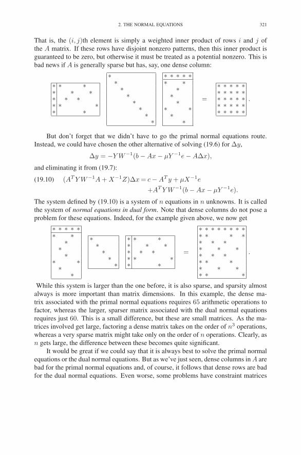
2. THE NORMAL EQUATIONS 321
That is, the (i, j)th element is simply a weighted inner product of rows i and j of
the A matrix. If these rows have disjoint nonzero patterns, then this inner product is
guaranteed to be zero, but otherwise it must be treated as a potential nonzero. This is
bad news if A is generally sparse but has, say, one dense column:
∗ ∗ ∗∗ ∗ ∗∗ ∗ ∗∗ ∗ ∗∗ ∗
∗∗∗∗∗∗∗∗
∗ ∗ ∗ ∗ ∗∗ ∗
∗∗∗
∗ ∗∗
∗
=
∗ ∗ ∗ ∗ ∗∗ ∗ ∗ ∗ ∗∗ ∗ ∗ ∗ ∗∗ ∗ ∗ ∗ ∗∗ ∗ ∗ ∗ ∗
.
But don’t forget that we didn’t have to go the primal normal equations route.
Instead, we could have chosen the other alternative of solving (19.6) for ∆y,
∆y = −Y W−1(b − Ax − μY −1e − A∆x),
and eliminating it from (19.7):
(AT Y W−1A + X−1Z)∆x = c − AT y + μX−1e(19.10)
+AT Y W−1(b − Ax − μY −1e).
The system defined by (19.10) is a system of n equations in n unknowns. It is called
the system of normal equations in dual form. Note that dense columns do not pose a
problem for these equations. Indeed, for the example given above, we now get
∗ ∗ ∗ ∗ ∗∗ ∗
∗∗∗
∗ ∗∗
∗
∗∗∗∗∗
∗ ∗ ∗∗ ∗ ∗∗ ∗ ∗∗ ∗ ∗∗ ∗
=
∗ ∗ ∗ ∗ ∗ ∗ ∗ ∗∗ ∗ ∗ ∗∗ ∗ ∗∗ ∗ ∗∗ ∗ ∗∗ ∗ ∗∗ ∗ ∗∗ ∗ ∗
.
While this system is larger than the one before, it is also sparse, and sparsity almost
always is more important than matrix dimensions. In this example, the dense ma-
trix associated with the primal normal equations requires 65 arithmetic operations to
factor, whereas the larger, sparser matrix associated with the dual normal equations
requires just 60. This is a small difference, but these are small matrices. As the ma-
trices involved get large, factoring a dense matrix takes on the order of n3 operations,
whereas a very sparse matrix might take only on the order of n operations. Clearly, as
n gets large, the difference between these becomes quite significant.
It would be great if we could say that it is always best to solve the primal normal
equations or the dual normal equations. But as we’ve just seen, dense columns in A are
bad for the primal normal equations and, of course, it follows that dense rows are bad
for the dual normal equations. Even worse, some problems have constraint matrices

322 19. THE KKT SYSTEM
A that are overall very sparse but contain some dense rows and some dense columns.
Such problems are sure to run into trouble with either sets of normal equations. For
these reasons, it is best to factor the matrix in the reduced KKT system directly. Then
it is possible to find pivot orders that circumvent the difficulties posed by both dense
columns and dense rows.
3. Step Direction Decomposition
In the next chapter, we shall discuss factorization techniques for symmetric ma-
trices (along with other implementation issues). However, before we embark on that
discussion, we end this chapter by taking a closer look at the formulas for the step
direction vectors. To be specific, let us look at ∆x. From the primal normal equa-
tions (19.9), we can solve for ∆y and then substitute the solution into (19.8) to get an
explicit formula for ∆x:
∆x =(
D2 − D2AT (E−2 + AD2AT )−1AD2)
(c − AT y + μX−1e)(19.11)
+ D2AT (E−2 + AD2AT )−1(b − Ax − μY −1e),
where we have denoted by D the positive diagonal matrix defined by
D2 = XZ−1
and we have denoted by E the positive diagonal matrix defined by
E2 = Y W−1
(defining these matrices by their squares is possible, since the squares have positive
diagonal entries). However, using the dual normal equations, we get
∆x =(
AT E2A + D−2)−1
(c − AT y + μX−1e)(19.12)
+(
AT E2A + D−2)−1
AT E2(b − Ax − μY −1e).
These two expressions for ∆x look entirely different, but they must be the same, since
we know that ∆x is uniquely defined by the reduced KKT system. They are indeed
the same, as can be shown directly by establishing a certain matrix identity. This is
the subject of Exercise 19.1. There are a surprising number of published research
papers on interior-point methods that present supposedly new algorithms that are in
fact identical to existing methods. These papers get published because the equivalence
is not immediately obvious (such as the one we just established).
3. STEP DIRECTION DECOMPOSITION 323
We can gain further insight into the path-following method by looking more
closely at the primal step direction vector. Formula (19.11) can be rearranged as fol-
lows:
∆x =(
D2 − D2AT (E−2 + AD2AT )−1AD2)
c
+ μ(
D2 − D2AT (E−2 + AD2AT )−1AD2)
X−1e
− μD2AT (E−2 + AD2AT )−1Y −1e
+ D2AT (E−2 + AD2AT )−1(b − Ax)
− D2AT(
I − (E−2 + AD2AT )−1AD2AT)
y.
For comparison purposes down the road, we prefer to write the Y −1e that appears in
the second term containing μ as E−2W−1e. Also, using the result of Exercise 19.2,
we can rewrite the bulk of the last line as follows:(
I − (E−2 + AD2AT )−1AD2AT)
y = (E−2 + AD2AT )−1E−2y
= (E−2 + AD2AT )−1w.
Putting this all together, we get
∆x =(
D2 − D2AT (E−2 + AD2AT )−1AD2)
c
+ μ(
D2 − D2AT (E−2 + AD2AT )−1AD2)
X−1e
− μD2AT (E−2 + AD2AT )−1E−2W−1e
+ D2AT (E−2 + AD2AT )−1ρ
=∆xOPT + μ∆xCTR + ∆xFEAS,
where
∆xOPT =(
D2 − D2AT (E−2 + AD2AT )−1AD2)
c,
∆xCTR =(
D2 − D2AT (E−2 + AD2AT )−1AD2)
X−1e
− D2AT (E−2 + AD2AT )−1E−2W−1e,
and
∆xFEAS = D2AT (E−2 + AD2AT )−1ρ.
In Chapter 21, we shall show that these components of ∆x have important connections
to the step directions that arise in a related interior-point method called the affine-
scaling method. For now, we simply establish some of their properties as they relate
to the path-following method. Our first result is that ∆xOPT is an ascent direction.
THEOREM 19.1. cT ∆xOPT ≥ 0.
PROOF. We use the result of Exercise 19.1 (with the roles of E and D switched)
to see that
∆xOPT = (AT E2A + D−2)−1c.

324 19. THE KKT SYSTEM
Hence,
cT ∆xOPT = cT (AT E2A + D−2)−1c.
We claim that the right-hand side is obviously nonnegative, since the matrix sand-
wiched between c and its transpose is positive semidefinite.1 Indeed, the claim follows
from the definition of positive semidefiniteness: a matrix B is positive semidefinite if
ξT Bξ ≥ 0 for all vectors ξ. To see that the matrix in question is in fact positive
semidefinite, we first note that AT E2A and D−2 are positive semidefinite:
ξT AT E2Aξ = ‖EAξ‖2 ≥ 0 and ξT D−2ξ = ‖D−1ξ‖2 ≥ 0.
Then we show that the sum of two positive semidefinite matrices is positive semidefi-
nite and finally that the inverse of a symmetric positive semidefinite matrix is positive
semidefinite. To verify closure under summation, suppose that B(1) and B(2) are pos-
itive semidefinite, and then compute
ξT (B(1) + B(2))ξ = ξT B(1)ξ + ξT B(2)ξ ≥ 0.
To verify closure under forming inverses of symmetric positive semidefinite matrices,
suppose that B is symmetric and positive semidefinite. Then
ξT B−1ξ = ξT B−1BB−1ξ = (B−1ξ)T B(B−1ξ) ≥ 0,
where the inequality follows from the fact that B is positive semidefinite and B−1ξ is
simply any old vector. This completes the proof. �
The theorem just proved justifies our referring to ∆xOPT as a step-toward-optimality
direction. We next show that ∆xFEAS is in fact a step-toward-feasibility.
In Exercise 19.3, you are asked to find the formulas for the primal slack vector’s
step directions, ∆wOPT, ∆wCTR, and ∆wFEAS. It is easy to verify from these formu-
las that the pairs (∆xOPT,∆wOPT) and (∆xCTR,∆wCTR) preserve the current level of
infeasibility. That is,
A∆xOPT + ∆wOPT = 0
and
A∆xCTR + ∆wCTR = 0.
Hence, only the “feasibility” directions can improve the degree of feasibility. Indeed,
it is easy to check that
A∆xFEAS + ∆wFEAS = ρ.
Finally, we consider ∆xCTR. If the objective function were zero (i.e., c = 0) and
if the current point were feasible, then steps toward optimality and feasibility would
vanish and we would be left with just ∆xCTR. Since our step directions were derived
in an effort to move toward a point on the central path parametrized by μ, we now see
that ∆xCTR plays the role of a step-toward-centrality.
1In fact, it’s positive definite, but we don’t need this stronger property here.

NOTES 325
Exercises
19.1 Sherman–Morrison–Woodbury Formula. Assuming that all the inverses be-
low exist, show that the following identity is true:
(E−1 + ADAT )−1 = E − EA(AT EA + D−1)−1AT E.
Use this identity to verify directly the equivalence of the expressions given
for ∆x in (19.11) and (19.12).
19.2 Assuming that all the inverses exist, show that the following identity holds:
I − (E + ADAT )−1ADAT = (E + ADAT )−1E.
19.3 Show that
∆w = ∆wOPT + μ∆wCTR + ∆wFEAS,
where
∆wOPT = −A(
D2 − D2AT (E−2 + AD2AT )−1AD2)
c,
∆wCTR = −A(
D2 − D2AT (E−2 + AD2AT )−1AD2)
X−1e
+ AD2AT (E−2 + AD2AT )−1E−2W−1e,
and
∆wFEAS = ρ − AD2AT (E−2 + AD2AT )−1ρ.
Notes
The KKT system for general inequality constrained optimization problems was
derived by Kuhn & Tucker (1951). It was later discovered that W. Karush had proven
the same result in his 1939 master’s thesis at the University of Chicago (Karush
1939). John (1948) was also an early contributor to inequality-constrained optimiza-
tion. Kuhn’s survey paper (Kuhn 1976) gives a historical account of the development
of the subject.


CHAPTER 20
Implementation Issues
In this chapter, we discuss implementation issues that arise in connection with the
path-following method.
The most important issue is the efficient solution of the systems of equations dis-
cussed in the previous chapter. As we saw, there are basically three choices, involving
either the reduced KKT matrix,
(20.1) B =
[
−E−2 A
AT D−2
]
,
or one of the two matrices associated with the normal equations:
(20.2) AD2AT + E−2
or
(20.3) AT E2A + D−2.
(Here, E−2 = Y −1W and D−2 = X−1Z.)
In the previous chapter, we explained that dense columns/rows are bad for the
normal equations and that therefore one might be better off solving the system involv-
ing the reduced KKT matrix. But there is also a reason one might prefer to work with
one of the systems of normal equations. The reason is that these matrices are posi-
tive definite. We shall show in the first section that there are important advantages in
working with positive definite matrices. In the second section, we shall consider the
reduced KKT matrix and see to what extent the nice properties possessed by positive
definite matrices carry over to these matrices.
After finishing our investigations into numerical factorization, we shall take up
a few other relevant tasks, such as how one extends the path-following algorithm to
handle problems with bounds and ranges.
1. Factoring Positive Definite Matrices
As we saw in the proof of Theorem 19.1, the matrix (20.2) appearing in the primal
normal equations is positive semidefinite (and so is (20.3), of course). In fact, it is
even better—it’s positive definite. A matrix B is positive definite if ξT Bξ > 0 for
all vectors ξ �= 0. In this section, we will show that, if we restrict our row/column
327

328 20. IMPLEMENTATION ISSUES
reordering to symmetric reorderings, that is, reorderings where the rows and columns
undergo the same permutation, then there is no danger of encountering a pivot element
whose value is zero. Hence, the row/column permutation can be selected ahead of time
based only on the aim of maintaining sparsity.
If we restrict ourselves to symmetric permutations, each pivot element is a diago-
nal element of the matrix. The following result shows that we can start by picking an
arbitrary diagonal element as the first pivot element:
THEOREM 20.1. If B is positive definite, then bii > 0 for all i.
The proof follows trivially from the definition of positive definiteness:
bii = eTi Bei > 0.
The next step is to show that after each stage of the elimination process, the remaining
uneliminated matrix is positive definite. Let us illustrate by breaking out the first
row/column of the matrix and looking at what the first step of the elimination process
does. Breaking out the first row/column, we write
B =
[
a bT
b C
]
.
Here, a is the first diagonal element (a scalar), b is the column below a, and C is the
matrix consisting of all of B except the first row/column. One step of elimination (as
described in Chapter 8) transforms B into[
a bT
b C − bbT
a
]
.
The following theorem tells us that the uneliminated part is positive definite:
THEOREM 20.2. If B is positive definite, then so is C − bbT /a.
PROOF. The fact that B is positive definite implies that
(20.4)[
x yT]
[
a bT
b C
][
x
y
]
= ax2 + 2yT bx + yT Cy
is positive whenever the scalar x or the vector y is nonzero (or both). Fix a vector
y �= 0, and put x = − 1abT y. Using these choices in (20.4), we get
0 <1
ayT bbT y − 2
1
ayT bbT y + yT Cy = yT
(
C − bbT
a
)
y.
Since y was an arbitrary nonzero vector, it follows that C − bbT /a is positive definite.
�

1. FACTORING POSITIVE DEFINITE MATRICES 329
Hence, after one step of the elimination, the uneliminated part is positive definite.
It follows by induction then that the uneliminated part is positive definite at every step
of the elimination.
Here’s an example:
B =
⎡
⎢
⎢
⎢
⎢
⎢
⎢
⎢
⎣
2 −1 −1
−1 3 −1 −1
−1 2 −1
−1 −1 3 −1
−1 −1 3
⎤
⎥
⎥
⎥
⎥
⎥
⎥
⎥
⎦
.
At the end of the four steps of the elimination (without permutations), we end up with⎡
⎢
⎢
⎢
⎢
⎢
⎢
⎢
⎣
2 −1 −1
−1 52 −1 −1 − 1
2
−1 85 − 7
5 − 15
−1 − 75
118 − 11
8
−1 − 12 − 1
5 − 118 1
⎤
⎥
⎥
⎥
⎥
⎥
⎥
⎥
⎦
.
From this eliminated form, we extract the lower triangular matrix, the diagonal matrix,
and the upper triangular matrix to write B as
B =
⎡
⎢
⎢
⎢
⎢
⎢
⎢
⎢
⎣
2
−1 52
−1 85
−1 − 75
118
−1 − 12 − 1
5 − 118 1
⎤
⎥
⎥
⎥
⎥
⎥
⎥
⎥
⎦
⎡
⎢
⎢
⎢
⎢
⎢
⎢
⎢
⎣
252
85
118
1
⎤
⎥
⎥
⎥
⎥
⎥
⎥
⎥
⎦
−1 ⎡
⎢
⎢
⎢
⎢
⎢
⎢
⎢
⎣
2 −1 −152 −1 −1 − 1
285 − 7
5 − 15
118 − 11
8
1
⎤
⎥
⎥
⎥
⎥
⎥
⎥
⎥
⎦
.
As we saw in Chapter 8, it is convenient to combine the lower triangular matrix with
the diagonal matrix to get a new lower triangular matrix with ones on the diagonal.
But the current lower triangular matrix is exactly the transpose of the upper triangular
matrix. Hence, to preserve symmetry, we should combine the diagonal matrix with
both the lower and the upper triangular matrices. Since it only appears once, we must
multiply and divide by it (in the middle of the product). Doing this, we get
B =
⎡
⎢
⎢
⎢
⎢
⎢
⎢
⎢
⎣
1
− 12 1
− 25 1
− 25 − 7
8 1
− 12 − 1
5 − 18 −1 1
⎤
⎥
⎥
⎥
⎥
⎥
⎥
⎥
⎦
⎡
⎢
⎢
⎢
⎢
⎢
⎢
⎢
⎣
252
85
118
1
⎤
⎥
⎥
⎥
⎥
⎥
⎥
⎥
⎦
⎡
⎢
⎢
⎢
⎢
⎢
⎢
⎢
⎣
1 − 12 − 1
2
1 − 25 − 2
5 − 15
1 − 78 − 1
8
1 −1
1
⎤
⎥
⎥
⎥
⎥
⎥
⎥
⎥
⎦
.
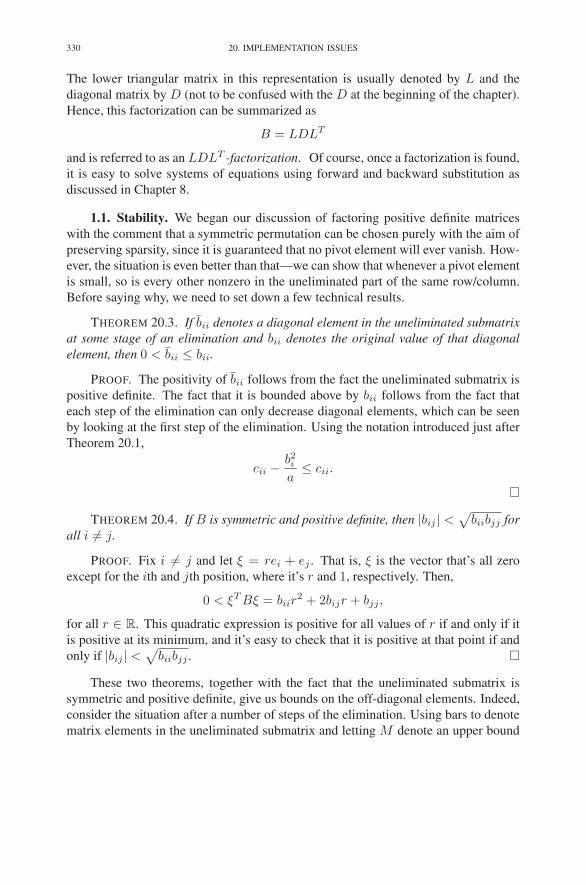
330 20. IMPLEMENTATION ISSUES
The lower triangular matrix in this representation is usually denoted by L and the
diagonal matrix by D (not to be confused with the D at the beginning of the chapter).
Hence, this factorization can be summarized as
B = LDLT
and is referred to as an LDLT -factorization. Of course, once a factorization is found,
it is easy to solve systems of equations using forward and backward substitution as
discussed in Chapter 8.
1.1. Stability. We began our discussion of factoring positive definite matrices
with the comment that a symmetric permutation can be chosen purely with the aim of
preserving sparsity, since it is guaranteed that no pivot element will ever vanish. How-
ever, the situation is even better than that—we can show that whenever a pivot element
is small, so is every other nonzero in the uneliminated part of the same row/column.
Before saying why, we need to set down a few technical results.
THEOREM 20.3. If bii denotes a diagonal element in the uneliminated submatrix
at some stage of an elimination and bii denotes the original value of that diagonal
element, then 0 < bii ≤ bii.
PROOF. The positivity of bii follows from the fact the uneliminated submatrix is
positive definite. The fact that it is bounded above by bii follows from the fact that
each step of the elimination can only decrease diagonal elements, which can be seen
by looking at the first step of the elimination. Using the notation introduced just after
Theorem 20.1,
cii −b2i
a≤ cii.
�
THEOREM 20.4. If B is symmetric and positive definite, then |bij | <√
biibjj for
all i �= j.
PROOF. Fix i �= j and let ξ = rei + ej . That is, ξ is the vector that’s all zero
except for the ith and jth position, where it’s r and 1, respectively. Then,
0 < ξT Bξ = biir2 + 2bijr + bjj ,
for all r ∈ R. This quadratic expression is positive for all values of r if and only if it
is positive at its minimum, and it’s easy to check that it is positive at that point if and
only if |bij | <√
biibjj . �
These two theorems, together with the fact that the uneliminated submatrix is
symmetric and positive definite, give us bounds on the off-diagonal elements. Indeed,
consider the situation after a number of steps of the elimination. Using bars to denote
matrix elements in the uneliminated submatrix and letting M denote an upper bound
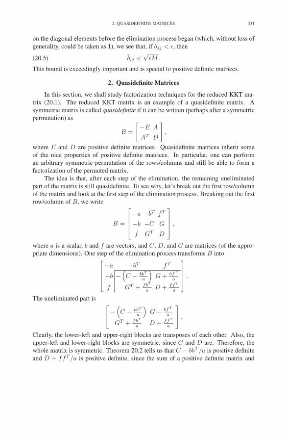
2. QUASIDEFINITE MATRICES 331
on the diagonal elements before the elimination process began (which, without loss of
generality, could be taken as 1), we see that, if bjj < ǫ, then
(20.5) bij <√
ǫM.
This bound is exceedingly important and is special to positive definite matrices.
2. Quasidefinite Matrices
In this section, we shall study factorization techniques for the reduced KKT ma-
trix (20.1). The reduced KKT matrix is an example of a quasidefinite matrix. A
symmetric matrix is called quasidefinite if it can be written (perhaps after a symmetric
permutation) as
B =
[
−E A
AT D
]
,
where E and D are positive definite matrices. Quasidefinite matrices inherit some
of the nice properties of positive definite matrices. In particular, one can perform
an arbitrary symmetric permutation of the rows/columns and still be able to form a
factorization of the permuted matrix.
The idea is that, after each step of the elimination, the remaining uneliminated
part of the matrix is still quasidefinite. To see why, let’s break out the first row/column
of the matrix and look at the first step of the elimination process. Breaking out the first
row/column of B, we write
B =
⎡
⎢
⎢
⎣
−a −bT fT
−b −C G
f GT D
⎤
⎥
⎥
⎦
,
where a is a scalar, b and f are vectors, and C, D, and G are matrices (of the appro-
priate dimensions). One step of the elimination process transforms B into⎡
⎢
⎢
⎣
−a −bT fT
−b −(
C − bbT
a
)
G + bfT
a
f GT + fbT
a D + ffT
a
⎤
⎥
⎥
⎦
.
The uneliminated part is⎡
⎣
−(
C − bbT
a
)
G + bfT
a
GT + fbT
a D + ffT
a
⎤
⎦ .
Clearly, the lower-left and upper-right blocks are transposes of each other. Also, the
upper-left and lower-right blocks are symmetric, since C and D are. Therefore, the
whole matrix is symmetric. Theorem 20.2 tells us that C − bbT /a is positive definite
and D + ffT /a is positive definite, since the sum of a positive definite matrix and

332 20. IMPLEMENTATION ISSUES
a positive semidefinite matrix is positive definite (see Exercise 20.2). Therefore, the
uneliminated part is indeed quasidefinite.
Of course, had the first pivot element been selected from the submatrix D instead
of E, perhaps the story would be different. But it is easy to check that it’s the same.
Hence, no matter which diagonal element is selected to be the first pivot element, the
resulting uneliminated part is quasidefinite. Now, by induction it follows that every
step of the elimination process involves choosing a pivot element from the diagonals
of a quasidefinite matrix. Since these diagonals come from either a positive definite
submatrix or the negative of such a matrix, it follows that they are always nonzero (but
many of them will be negative). Therefore, just as for positive definite matrices, an
arbitrary symmetric permutation of a quasidefinite matrix can be factored without any
risk of encountering a zero pivot element.
Here’s an example:
(20.6) B =
1 2 3 4 5
1
2
3
4
5
⎡
⎢
⎢
⎢
⎢
⎢
⎢
⎢
⎣
−1 −2 1
−2 2
−3 1
−2 1 2
1 2 1
⎤
⎥
⎥
⎥
⎥
⎥
⎥
⎥
⎦
.
(The blocks are easy to pick out, since the negative diagonals must be from −E,
whereas the positive ones are from D.) Let’s eliminate by picking the diagonals in the
order 1, 5, 2, 4, 3. No permutations are needed in preparation for the first step of the
elimination. After this step, we have
1 2 3 4 5
1
2
3
4
5
⎡
⎢
⎢
⎢
⎢
⎢
⎢
⎢
⎣
−1 −2 1
−2 2
−3 1
−2 1 6 −2
1 2 −2 2
⎤
⎥
⎥
⎥
⎥
⎥
⎥
⎥
⎦
.

2. QUASIDEFINITE MATRICES 333
Now, we move row/column 5 to the pivot position, slide the other rows/columns
down/over, and eliminate to get
1 5 2 3 4
1
5
2
3
4
⎡
⎢
⎢
⎢
⎢
⎢
⎢
⎢
⎣
−1 1 −2
1 2 2 −2
2 −4 2
−3 1
−2 −2 2 1 4
⎤
⎥
⎥
⎥
⎥
⎥
⎥
⎥
⎦
.
Row/column 2 is in the correct position for the third step of the elimination, and there-
fore, without further ado, we do the next step in the elimination:
1 5 2 3 4
1
5
2
3
4
⎡
⎢
⎢
⎢
⎢
⎢
⎢
⎢
⎣
−1 1 −2
1 2 2 −2
2 −4 2
−3 1
−2 −2 2 1 5
⎤
⎥
⎥
⎥
⎥
⎥
⎥
⎥
⎦
.
Finally, we interchange rows/columns 3 and 4 and do the last elimination step to get
1 5 2 4 3
1
5
2
4
3
⎡
⎢
⎢
⎢
⎢
⎢
⎢
⎢
⎣
−1 1 −2
1 2 2 −2
2 −4 2
−2 −2 2 5 1
1 − 165
⎤
⎥
⎥
⎥
⎥
⎥
⎥
⎥
⎦
.
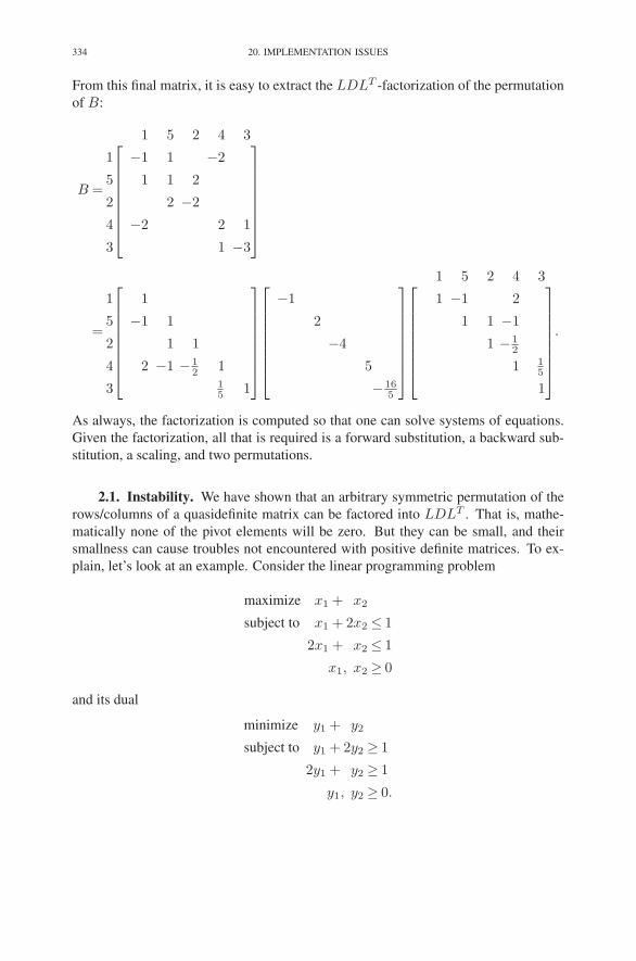
334 20. IMPLEMENTATION ISSUES
From this final matrix, it is easy to extract the LDLT -factorization of the permutation
of B:
B =
1 5 2 4 3
1
5
2
4
3
⎡
⎢
⎢
⎢
⎢
⎢
⎢
⎢
⎣
−1 1 −2
1 1 2
2 −2
−2 2 1
1 −3
⎤
⎥
⎥
⎥
⎥
⎥
⎥
⎥
⎦
=
1
5
2
4
3
⎡
⎢
⎢
⎢
⎢
⎢
⎢
⎢
⎣
1
−1 1
1 1
2 −1 − 12 1
15 1
⎤
⎥
⎥
⎥
⎥
⎥
⎥
⎥
⎦
⎡
⎢
⎢
⎢
⎢
⎢
⎢
⎢
⎣
−1
2
−4
5
− 165
⎤
⎥
⎥
⎥
⎥
⎥
⎥
⎥
⎦
1 5 2 4 3⎡
⎢
⎢
⎢
⎢
⎢
⎢
⎢
⎣
1 −1 2
1 1 −1
1 − 12
1 15
1
⎤
⎥
⎥
⎥
⎥
⎥
⎥
⎥
⎦
.
As always, the factorization is computed so that one can solve systems of equations.
Given the factorization, all that is required is a forward substitution, a backward sub-
stitution, a scaling, and two permutations.
2.1. Instability. We have shown that an arbitrary symmetric permutation of the
rows/columns of a quasidefinite matrix can be factored into LDLT . That is, mathe-
matically none of the pivot elements will be zero. But they can be small, and their
smallness can cause troubles not encountered with positive definite matrices. To ex-
plain, let’s look at an example. Consider the linear programming problem
maximize x1 + x2
subject to x1 + 2x2 ≤ 1
2x1 + x2 ≤ 1
x1, x2 ≥ 0
and its dual
minimize y1 + y2
subject to y1 + 2y2 ≥ 1
2y1 + y2 ≥ 1
y1, y2 ≥ 0.
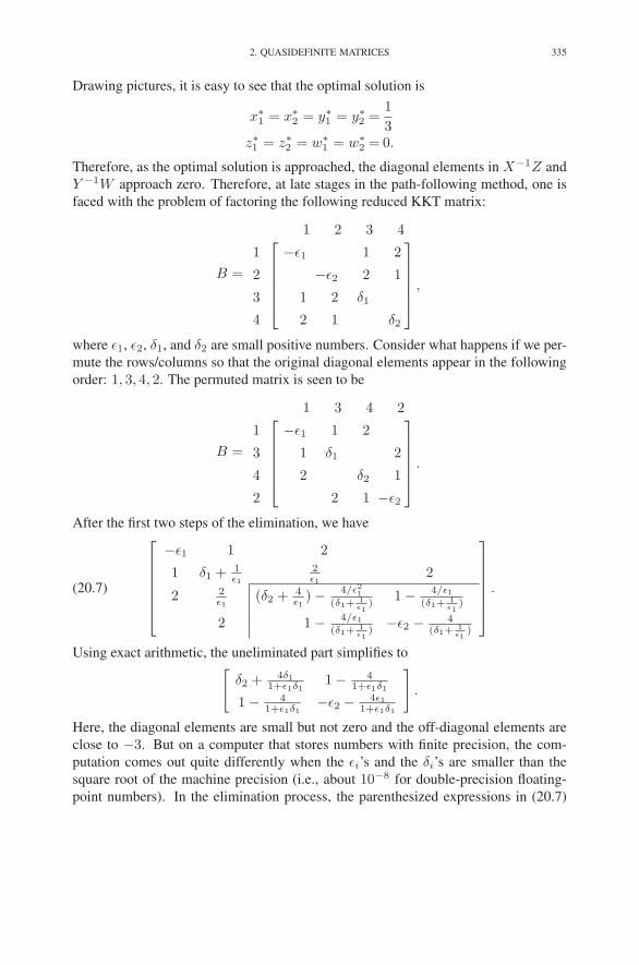
2. QUASIDEFINITE MATRICES 335
Drawing pictures, it is easy to see that the optimal solution is
x∗1 = x∗
2 = y∗1 = y∗
2 =1
3z∗1 = z∗2 = w∗
1 = w∗2 = 0.
Therefore, as the optimal solution is approached, the diagonal elements in X−1Z and
Y −1W approach zero. Therefore, at late stages in the path-following method, one is
faced with the problem of factoring the following reduced KKT matrix:
B =
1 2 3 4
1
2
3
4
⎡
⎢
⎢
⎢
⎢
⎣
−ǫ1 1 2
−ǫ2 2 1
1 2 δ1
2 1 δ2
⎤
⎥
⎥
⎥
⎥
⎦
,
where ǫ1, ǫ2, δ1, and δ2 are small positive numbers. Consider what happens if we per-
mute the rows/columns so that the original diagonal elements appear in the following
order: 1, 3, 4, 2. The permuted matrix is seen to be
B =
1 3 4 2
1
3
4
2
⎡
⎢
⎢
⎢
⎢
⎣
−ǫ1 1 2
1 δ1 2
2 δ2 1
2 1 −ǫ2
⎤
⎥
⎥
⎥
⎥
⎦
.
After the first two steps of the elimination, we have
(20.7)
⎡
⎢
⎢
⎢
⎢
⎢
⎣
−ǫ1 1 2
1 δ1 + 1ǫ1
2ǫ1
2
2 2ǫ1
(δ2 + 4ǫ1
) − 4/ǫ21(δ1+
1ǫ1
)1 − 4/ǫ1
(δ1+1
ǫ1)
2 1 − 4/ǫ1(δ1+
1ǫ1
)−ǫ2 − 4
(δ1+1
ǫ1)
⎤
⎥
⎥
⎥
⎥
⎥
⎦
.
Using exact arithmetic, the uneliminated part simplifies to[
δ2 + 4δ1
1+ǫ1δ11 − 4
1+ǫ1δ1
1 − 41+ǫ1δ1
−ǫ2 − 4ǫ11+ǫ1δ1
]
.
Here, the diagonal elements are small but not zero and the off-diagonal elements are
close to −3. But on a computer that stores numbers with finite precision, the com-
putation comes out quite differently when the ǫi’s and the δi’s are smaller than the
square root of the machine precision (i.e., about 10−8 for double-precision floating-
point numbers). In the elimination process, the parenthesized expressions in (20.7)

336 20. IMPLEMENTATION ISSUES
are evaluated before the other operations. Hence, in finite precision arithmetic, these
expressions produce
δ2 +4
ǫ1=
4
ǫ1and δ1 +
1
ǫ1=
1
ǫ1,
and so (20.7) becomes
1 3 4 2
1
3
4
2
⎡
⎢
⎢
⎢
⎢
⎣
−ǫ1 1 2
1 1ǫ1
2ǫ1
2
2 2ǫ1
0 −3
2 −3 −4ǫ1
⎤
⎥
⎥
⎥
⎥
⎦
,
which clearly presents a problem for the next step in the elimination process.
Now let’s consider what happens if the elimination process is applied directly to
B without permuting the rows/columns. Sparing the reader the tedious details, the end
result of the elimination is the following matrix:
(20.8)
⎡
⎢
⎢
⎢
⎢
⎢
⎣
−ǫ1 1 2
−ǫ2 2 1
1 2 δ1 + 1ǫ1
+ 4ǫ2
2ǫ1
+ 2ǫ2
2 1 2ǫ1
+ 2ǫ2
δ2 + 4ǫ1
+ 1ǫ2
− ( 2ǫ1
+ 2ǫ2
)2
(δ1+1
ǫ1+ 4
ǫ2)
⎤
⎥
⎥
⎥
⎥
⎥
⎦
.
As before, in finite precision arithmetic, certain small numbers get lost:
δ2 +4
ǫ1=
4
ǫ1and δ1 +
1
ǫ1=
1
ǫ1.
Making these substitutions in (20.8), we see that the final matrix produced by the
elimination process using finite precision arithmetic is⎡
⎢
⎢
⎢
⎢
⎣
−ǫ1 1 2
−ǫ2 2 1
1 2 1ǫ1
+ 4ǫ2
2ǫ1
+ 2ǫ2
2 1 2ǫ1
+ 2ǫ2
0
⎤
⎥
⎥
⎥
⎥
⎦
.
Just as before, the fact that small numbers got lost has resulted in a zero appearing
on the diagonal where a small but nonzero (in this case positive) number belongs.
However, the situation is fundamentally different this time. With the first ordering,
a −3 remained to be eliminated under the zero diagonal element, whereas with the
second ordering, this did not happen. Of course, it didn’t happen in this particular
example because the 0 appeared as the last pivot element, which has no elements below
it to be eliminated. But that is not the general reason why the second ordering does
3. PROBLEMS IN GENERAL FORM 337
not produce nonzeros under zero pivot elements. In general, a zero (which should be
a small positive) can appear anywhere in the lower-right block (relative to the original
quasidefinite partitioning). But once the elimination process gets to this block, the
remaining uneliminated part of the matrix is positive definite. Hence, the estimate in
(20.5) can be used to tell us that all the nonzeros below a zero diagonal are in fact
small themselves. A zero appearing on the diagonal only presents a problem if there
are nonzeros below it that need to be eliminated. If there are none, then the elimination
can simply proceed to the next pivot element (see Exercise 20.1).
Let’s summarize the situation. We showed in the last chapter that the possibility of
dense rows/columns makes it unattractive to work strictly with the normal equations.
Yet, although the quasidefinite reduced KKT system can be used, it is numerically
less stable. A compromise solution seems to be suggested. One could take a struc-
tured approach to the reordering heuristic. In the structured approach, one decides first
whether it seems better to begin pivoting with elements from the upper-left block or
from the lower-right block. Once this decision is made, one should pivot out all the
diagonal elements from this block before working on the other block, with the excep-
tion that pivots involving dense rows/columns be deferred to the end of the elimination
process. If no dense columns are identified, this strategy mimics the normal equations
approach. Indeed, after eliminating all the diagonal elements in the upper-left block,
the remaining uneliminated lower-right block contains exactly the matrix for the sys-
tem of dual normal equations. Similarly, had the initial choice been to pivot out all
the diagonal elements from the lower-right block, then the remaining uneliminated
upper-left block becomes the matrix for the system of primal normal equations.
With this structured approach, if no dense rows/columns are identified and de-
ferred, then the elimination process is numerically stable. If, on the other hand, some
dense rows/columns are deferred, then the factorization is less stable. But in practice,
this approach seems to work well. Of course, one could be more careful and monitor
the diagonal elements. If a diagonal element gets small (relative to the other unelim-
inated nonzeros in the same row/column), then one could flag it and then calculate a
new ordering in which such pivot elements are deferred to the end of the elimination
process.
3. Problems in General Form
In this section, we describe how to adapt the path-following algorithm to solving
problems presented in the following general form:
(20.9)
maximize cT x
subject to a ≤ Ax ≤ b
l ≤ x ≤ u.

338 20. IMPLEMENTATION ISSUES
As in Chapter 9, some of the data elements are allowed to take on infinite values.
However, let us consider first the case where all the components of a, b, l, and u are
finite. Infinities require special treatment, which shall be discussed shortly.
Following the derivation of the path-following method that we introduced in Chap-
ter 18, the first step is to introduce slack variables as appropriate to replace all inequal-
ity constraints with simple nonnegativity constraints. Hence, we rewrite the primal
problem (20.9) as follows:
maximize cT x
subject to Ax + f = b
−Ax + p = −a
x + t = u
−x + g = −l
f, p, t, g ≥ 0.
In Chapter 9, we showed that the dual problem is given by
minimize bT v − aT q + uT s − lT h
subject to AT (v − q) − (h − s) = c
v, q, s, h ≥ 0,
and the corresponding complementarity conditions are given by
fivi = 0 i = 1, 2, . . . ,m,
piqi = 0 i = 1, 2, . . . ,m,
tjsj = 0 j = 1, 2, . . . , n,
gjhj = 0 j = 1, 2, . . . , n.
The next step in the derivation is to introduce the primal–dual central path, which
we parametrize as usual by a positive real parameter μ. Indeed, for each μ > 0,
we define the associated central-path point in primal–dual space as the unique point
that simultaneously satisfies the conditions of primal feasibility, dual feasibility, and

3. PROBLEMS IN GENERAL FORM 339
μ-complementarity. Ignoring nonnegativity (which is enforced separately), these con-
ditions are
Ax + f = b
f + p = b − a
x + t = u
−x + g =−l
AT y + s − h = c
y + q − v = 0
FV e = μe
PQe = μe
TSe = μe
GHe = μe.
Note that we have replaced the primal feasibility condition, −Ax + p = −a, with the
equivalent condition that f +p = b−a, and we have introduced into the dual problem
new variables y defined by y = v − q. The reason for these changes is to put the
system of equations into a form in which A and AT appear as little as possible (so that
solving the system of equations for the step direction will be as efficient as possible).
The last four equations are the μ-complementarity conditions. As usual, each
upper case letter that appears on the left in these equations denotes the diagonal matrix
having the components of the corresponding lower-case vector on its diagonal. The
system is a nonlinear system of 5n + 5m equations in 5n + 5m unknowns. It has a
unique solution in the strict interior of the following subset of primal–dual space:
(20.10) {(x, f, p, t, g, y, v, q, s, h) : f, p, t, g, v, q, s, h ≥ 0}.This fact can be seen by noting that these equations are the first-order optimality con-
ditions for an associated strictly convex barrier problem.
As μ tends to zero, the central path converges to the optimal solution to both the
primal and dual problems. The path-following algorithm is defined as an iterative pro-
cess that starts from a point in the strict interior of (20.10), estimates at each iteration
a value of μ representing a point on the central path that is in some sense closer to the
optimal solution than the current point, and then attempts to step toward this central-
path point, making sure that the new point remains in the strict interior of the the set
given in (20.10).
Suppose for the moment that we have already decided on the target value for
μ. Let (x, . . . , h) denote the current point in the strict interior of (20.10), and let
(x+∆x, . . . , h+∆h) denote the point on the central path corresponding to the target

340 20. IMPLEMENTATION ISSUES
value of μ. The defining equations for the point on the central path can be written as
A∆x + ∆f = b − Ax − f =: ρ
∆f + ∆p = b − a − f − p =: α
∆x + ∆t = u − x − t =: τ
−∆x + ∆g = −l + x − g =: ν
AT ∆y + ∆s − ∆h = c − AT y − s + h =: σ
∆y + ∆q − ∆v = −y − q + v =: β
FV −1∆v + ∆f = μV −1e − f − V −1∆V ∆f =: γf
QP−1∆p + ∆q = μP−1e − q − P−1∆P∆q =: γq
ST−1∆t + ∆s = μT−1e − s − T−1∆T∆s =: γs
HG−1∆g + ∆h = μG−1e − h − G−1∆G∆h =: γh,
where we have introduced notations ρ, . . . , γh as shorthands for the right-hand side ex-
pressions. This is almost a linear system for the direction vectors (∆x, . . . ,∆h). The
only nonlinearities appear on the right-hand sides of the complementarity equations
(i.e., in γf , . . . , γh). As we saw before, Newton’s method suggests that we simply
drop these nonlinear terms to obtain a linear system for the “delta” variables.
Clearly, the main computational burden is to solve the system shown above. It
is important to note that this is a large, sparse, indefinite, linear system. It is also
symmetric if one negates certain rows and rearranges rows and columns appropriately:⎡
⎢
⎢
⎢
⎢
⎢
⎢
⎢
⎢
⎢
⎢
⎢
⎢
⎢
⎢
⎢
⎢
⎢
⎢
⎢
⎢
⎣
−FV −1 −I
I I
−I I
I I
A I
I −I AT
−I I I
I QP−1
I HG−1
I ST−1
⎤
⎥
⎥
⎥
⎥
⎥
⎥
⎥
⎥
⎥
⎥
⎥
⎥
⎥
⎥
⎥
⎥
⎥
⎥
⎥
⎥
⎦
⎡
⎢
⎢
⎢
⎢
⎢
⎢
⎢
⎢
⎢
⎢
⎢
⎢
⎢
⎢
⎢
⎢
⎢
⎢
⎢
⎢
⎣
∆v
∆s
∆h
∆q
∆y
∆x
∆f
∆p
∆g
∆t
⎤
⎥
⎥
⎥
⎥
⎥
⎥
⎥
⎥
⎥
⎥
⎥
⎥
⎥
⎥
⎥
⎥
⎥
⎥
⎥
⎥
⎦
=
⎡
⎢
⎢
⎢
⎢
⎢
⎢
⎢
⎢
⎢
⎢
⎢
⎢
⎢
⎢
⎢
⎢
⎢
⎢
⎢
⎢
⎣
−γf
τ
ν
α
ρ
σ
β
γq
γh
γs
⎤
⎥
⎥
⎥
⎥
⎥
⎥
⎥
⎥
⎥
⎥
⎥
⎥
⎥
⎥
⎥
⎥
⎥
⎥
⎥
⎥
⎦
.
Because this system is symmetric, we look for symmetric pivots to solve it. That
is, we choose our pivots only from the diagonal elements. It turns out that we can
eliminate ∆v, ∆p, ∆g, and ∆t using the nonzero diagonals −FV −1, QP−1, HG−1,
and ST−1, respectively, in any order without causing any nondiagonal fill-in. Indeed,

3. PROBLEMS IN GENERAL FORM 341
the equations for ∆v, ∆p, ∆g, and ∆t are
∆v = V F−1(γf − ∆f)
∆p = PQ−1(γq − ∆q)(20.11)
∆g = GH−1(γh − ∆h)
∆t = TS−1(γs − ∆s),
and after elimination from the system, we get⎡
⎢
⎢
⎢
⎢
⎢
⎢
⎢
⎢
⎢
⎣
−TS−1 I
−GH−1 −I
−PQ−1 I
A I
I −I AT
I I V F−1
⎤
⎥
⎥
⎥
⎥
⎥
⎥
⎥
⎥
⎥
⎦
⎡
⎢
⎢
⎢
⎢
⎢
⎢
⎢
⎢
⎢
⎣
∆s
∆h
∆q
∆y
∆x
∆f
⎤
⎥
⎥
⎥
⎥
⎥
⎥
⎥
⎥
⎥
⎦
=
⎡
⎢
⎢
⎢
⎢
⎢
⎢
⎢
⎢
⎢
⎣
τ
ν
α
ρ
σ
β
⎤
⎥
⎥
⎥
⎥
⎥
⎥
⎥
⎥
⎥
⎦
,
where again we have introduced abbreviated notations for the components of the right-
hand side:
τ = τ − TS−1γs
ν = ν − GH−1γh
α = α − PQ−1γq
β = β + V F−1γf .
Next we use the pivot elements −TS−1, −GH−1, and −PQ−1 to solve for ∆s,
∆h, and ∆q, respectively:
∆s = −ST−1(τ − ∆x)
∆h = −HG−1(ν + ∆x)(20.12)
∆q = −QP−1(α − ∆f).
After eliminating these variables, the system simplifies to⎡
⎢
⎢
⎣
A I
AT D
I E
⎤
⎥
⎥
⎦
⎡
⎢
⎢
⎣
∆y
∆x
∆f
⎤
⎥
⎥
⎦
=
⎡
⎢
⎢
⎣
ρ
σ + ST−1τ − HG−1ν
β + QP−1α.
⎤
⎥
⎥
⎦
,
where
D = ST−1 + HG−1
and
E = V F−1 + QP−1.

342 20. IMPLEMENTATION ISSUES
Finally, we use the pivot element E to solve for ∆f ,
(20.13) ∆f = E−1(β + QP−1α − ∆y),
which brings us to the reduced KKT equations:
(20.14)
[
−E−1 A
AT D
][
∆y
∆x
]
=
[
ρ − E−1(β + QP−1α)
σ + ST−1τ − HG−1ν
]
.
Up to this point, none of the eliminations have produced any off-diagonal fill-
in. Also, the matrix for system given in (20.14) is a symmetric quasidefinite matrix.
Hence, the techniques given in Section 19.2 for solving such systems can be used. The
algorithm is summarized in 20.1.
Exercises
20.1 The matrix
B =
⎡
⎢
⎢
⎢
⎢
⎢
⎢
⎢
⎣
2 −2
1 −1
−2 2
−1 2 −1
−1 2
⎤
⎥
⎥
⎥
⎥
⎥
⎥
⎥
⎦
is not positive definite but is positive semidefinite. Find a factorization B =LDLT , where L is lower triangular with ones on the diagonal and D is a
diagonal matrix with nonnegative diagonal elements. If such a factorization
exists for every symmetric positive semidefinite matrix, explain why. If not,
give a counterexample.
20.2 Show that the sum of a positive definite matrix and a positive semidefinite
matrix is positive definite.
20.3 Permute the rows/columns of the matrix B given in (20.6) so that the diag-
onal elements from B appear in the order 2, 3, 4, 5, 1. Compute an LDLT -
factorization of this matrix.
20.4 Show that, if B is symmetric and positive semidefinite, then |bij | ≤√
biibjj
for all i, j.
Notes
Most implementations of interior-point methods assume the problem to be formu-
lated with equality constraints. In this formulation, Lustig et al. (1994) give a good
overview of the performance of interior-point algorithms compared with the simplex
method.

NOTES 343
initialize (x, f, p, t, g, y, v, q, s, h) such that f, p, t, g, v, q, s, h > 0
while (not optimal) {
ρ = b − Ax − w
σ = c − AT y + z
γ = fT v + pT q + tT s + gT h
µ = δγ
n + mγf = µV −1e − f
γq = µP−1e − q
γs = µT−1e − s
γh = µG−1e − h
τ = u − x − t − TS−1γs
ν = −l + x − g − GH−1γh
α = b − a − f − p − PQ−1γq
β = −y − q + v + V F−1γf
D = ST−1 + HG−1
E = V F−1 + QP−1
solve:
[
−E−1 A
AT D
] [
∆y
∆x
]
=
[
ρ − E−1(β + QP−1α)
σ + ST−1τ − HG−1ν
]
compute: ∆f using (20.13), ∆s, ∆h, ∆q using (20.12),
and ∆v, ∆p, ∆g, ∆t using (20.11)
θ = r
(
maxij
{
−∆fj
fj
,−∆pi
pi
,−∆ti
ti
,−∆gj
gj
,
−∆vj
vj
,−∆qi
qi
,−∆si
si
,−∆hj
hj
})
−1
∧ 1
x ← x + θ∆x, y ← y + θ∆y, f ← f + θ∆f, v ← v + θ∆v
p ← p + θ∆p, q ← q + θ∆q, t ← t + θ∆t, s ← s + θ∆s
g ← g + θ∆g, h ← h + θ∆h
}
FIGURE 20.1. The path-following method—general form.

344 20. IMPLEMENTATION ISSUES
The suggestion that it is better to solve equations in the KKT form instead of
normal form was offered independently by a number of researchers (Gill et al. 1992,
Turner 1991, Fourer & Mehrotra 1991, Vanderbei & Carpenter 1993).
The advantages of the primal–dual symmetric formulation were first reported in
Vanderbei (1994). The basic properties of quasidefinite matrices were first given in
Vanderbei (1995).

CHAPTER 21
The Affine-Scaling Method
In the previous chapter, we showed that the step direction for the path-following
method can be decomposed into a linear combination of three directions: a direction
toward optimality, a direction toward feasibility, and a direction toward centrality. It
turns out that these directions, or minor variants of them, arise in all interior-point
methods.
Historically, one of the first interior-point methods to be invented, analyzed, and
implemented was a two-phase method in which Phase I uses only the feasibility di-
rection and Phase II uses only the optimality direction. This method is called affine
scaling. While it is no longer considered the method of choice for practical implemen-
tations, it remains important because its derivation provides valuable insight into the
nature of the three basic directions mentioned above.
In this chapter, we shall explain the affine-scaling principle and use it to derive
the step toward optimality and step toward feasibility directions. As always, our main
interest lies in problems presented in standard form. But for affine scaling, it is easier
to start by considering problems in equality form. Hence, we begin by assuming that
the linear programming problem is given as
(21.1)
maximize cT x
subject to Ax = b
x≥ 0.
We shall begin with the Phase II algorithm. Hence, we assume that we have a feasible
initial starting point, x0. For the affine-scaling method, it is important that this starting
point lie in the strict interior of the feasible set. That is, we assume that
Ax0 = b and x0 > 0.
1. The Steepest Ascent Direction
Since the affine-scaling principle is fundamentally geometric, it is useful to keep
a picture in mind. A typical picture for m = 1 and n = 3 is shown in Figure 21.1. The
ultimate goal is, of course, to move from x0 to the optimal solution x∗. However, the
short-term goal is to move from x0 in some direction ∆x that improves the objective
function. Such a direction is called an ascent direction. You probably recall from
345
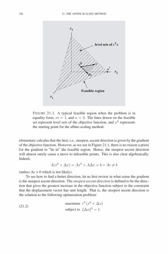
346 21. THE AFFINE-SCALING METHOD
x1
x2
x3
x0
level sets of cTx
Feasible region
x*
c
Pc
FIGURE 21.1. A typical feasible region when the problem is in
equality form, m = 1, and n = 3. The lines drawn on the feasible
set represent level sets of the objective function, and x0 represents
the starting point for the affine-scaling method.
elementary calculus that the best, i.e., steepest, ascent direction is given by the gradient
of the objective function. However, as we see in Figure 21.1, there is no reason a priori
for the gradient to “lie in” the feasible region. Hence, the steepest ascent direction
will almost surely cause a move to infeasible points. This is also clear algebraically.
Indeed,
A(x0 + ∆x) = Ax0 + A∆x = b + Ac �= b
(unless Ac = 0 which is not likely).
To see how to find a better direction, let us first review in what sense the gradient
is the steepest ascent direction. The steepest ascent direction is defined to be the direc-
tion that gives the greatest increase in the objective function subject to the constraint
that the displacement vector has unit length. That is, the steepest ascent direction is
the solution to the following optimization problem:
(21.2)maximize cT (x0 + ∆x)
subject to ‖∆x‖2 = 1.
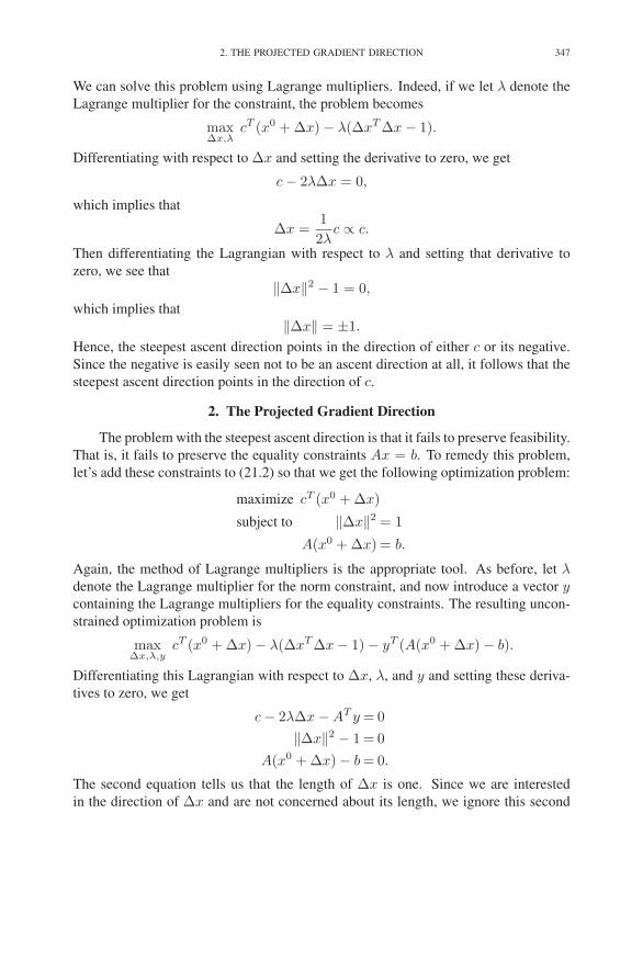
2. THE PROJECTED GRADIENT DIRECTION 347
We can solve this problem using Lagrange multipliers. Indeed, if we let λ denote the
Lagrange multiplier for the constraint, the problem becomes
max∆x,λ
cT (x0 + ∆x) − λ(∆xT ∆x − 1).
Differentiating with respect to ∆x and setting the derivative to zero, we get
c − 2λ∆x = 0,
which implies that
∆x =1
2λc ∝ c.
Then differentiating the Lagrangian with respect to λ and setting that derivative to
zero, we see that
‖∆x‖2 − 1 = 0,
which implies that
‖∆x‖ = ±1.
Hence, the steepest ascent direction points in the direction of either c or its negative.
Since the negative is easily seen not to be an ascent direction at all, it follows that the
steepest ascent direction points in the direction of c.
2. The Projected Gradient Direction
The problem with the steepest ascent direction is that it fails to preserve feasibility.
That is, it fails to preserve the equality constraints Ax = b. To remedy this problem,
let’s add these constraints to (21.2) so that we get the following optimization problem:
maximize cT (x0 + ∆x)
subject to ‖∆x‖2 = 1
A(x0 + ∆x) = b.
Again, the method of Lagrange multipliers is the appropriate tool. As before, let λdenote the Lagrange multiplier for the norm constraint, and now introduce a vector ycontaining the Lagrange multipliers for the equality constraints. The resulting uncon-
strained optimization problem is
max∆x,λ,y
cT (x0 + ∆x) − λ(∆xT ∆x − 1) − yT (A(x0 + ∆x) − b).
Differentiating this Lagrangian with respect to ∆x, λ, and y and setting these deriva-
tives to zero, we get
c − 2λ∆x − AT y = 0
‖∆x‖2 − 1 = 0
A(x0 + ∆x) − b = 0.
The second equation tells us that the length of ∆x is one. Since we are interested
in the direction of ∆x and are not concerned about its length, we ignore this second

348 21. THE AFFINE-SCALING METHOD
equation. The first equation tells us that ∆x is proportional to c − AT y, and again,
since we aren’t concerned about lengths, we put λ = 1/2 so that the first equation
reduces to
(21.3) ∆x = c − AT y.
Since Ax0 = b, the third equation says that
A∆x = 0.
Substituting (21.3) into this equation, we get
Ac − AAT y = 0,
which, assuming that AAT has full rank (as it should), can be solved for y to get
y = (AAT )−1Ac.
Now, substituting this expression into (21.3), we see that
∆x = c − AT (AAT )−1Ac.
It is convenient to let P be the matrix defined by
P = I − AT (AAT )−1A.
With this definition, ∆x can be expressed succinctly as
∆x = Pc.
We claim that P is the matrix that maps any vector, such as c, to its orthogonal
projection onto the null space of A. To justify this claim, we first need to define some
of the terms we’ve used. The null space of A is defined as {d ∈ Rn : Ad = 0}. We
shall denote the null space of A by N(A). A vector c is the orthogonal projection of
c onto N(A) if it lies in the null space,
c ∈ N(A),
and if the difference between it and c is orthogonal to every other vector in N(A).That is,
dT (c − c) = 0, for all d ∈ N(A).
Hence, to show that Pc is the orthogonal projection of c onto the null space of A, we
simply check these two conditions. Checking the first, we see that
APc = Ac − AAT (AAT )−1Ac,
which clearly vanishes. To check the second condition, let d be an arbitrary vector in
the null space, and compute
dT (c − Pc) = dT AT (AAT )−1Ac,
which also vanishes, since dT AT = (Ad)T = 0. The orthogonal projection Pc is
shown in Figure 21.1.

3. THE PROJECTED GRADIENT DIRECTION WITH SCALING 349
3. The Projected Gradient Direction with Scaling
The orthogonal projection of the gradient gives a good step direction in the sense
that among all feasibility-preserving directions, it gives the largest rate of increase
of cT x per unit step length. This property is nice as long as the current point x0 is
well inside the feasible set. But if it is close to a “wall,” the overall increase in one
step will be small, since even though the rate is large the actual step length will be
small, yielding a small overall increase. In fact, the increase will become arbitrarily
small as the point x0 is taken closer and closer to a “wall.” Hence, to get a reasonable
algorithm, we need to find a formula for computing step directions that steers away
from walls as they get close.
The affine-scaling algorithm achieves this affect as follows: scale the variables
in the problem so that the current feasible solution is far from the walls, compute the
step direction as the projected gradient in the scaled problem, and then translate this
direction back into the original system. The idea of scaling seems too simple to do
any good, and this is true if one tries the most naive scaling—just multiplying every
variable by one large number (such as the reciprocal of the smallest component of x0).
Such a uniform scaling does not change the picture in any way. For example, Figure
21.1, which doesn’t show specific scales on the coordinate axes, would not change at
all. Hence, whether distance is measured in miles or in feet, the property of being
close to a wall remains unchanged.
Fortunately, the scaling we have in mind for the affine-scaling algorithm is just
slightly fancier. Indeed, the idea is to scale each variable in such a manner that its
initial value gets mapped to 1. That is, for each j = 1, 2, . . . , n, we introduce new
variables given by
ξj =xj
x0j
.
Of course, this change of variable is trivial to undo:
xj = x0jξj .
In matrix notation, the change of variables can be written as
(21.4) x = X0ξ.
Note that we are employing our usual convention of letting an upper-case letter stand
for a diagonal matrix whose diagonal elements come from the components of the
vector denoted by the corresponding lower-case letter. Clearly, under this change of
variables, the initial solution x0 gets mapped to the vector e of all ones, which is at
least one unit away from each wall. Figure 21.2 shows an example of this scaling
transformation. Note that, unlike the trivial scaling mentioned above, this scaling
changes the way the level sets of the objective cut across the feasible region.
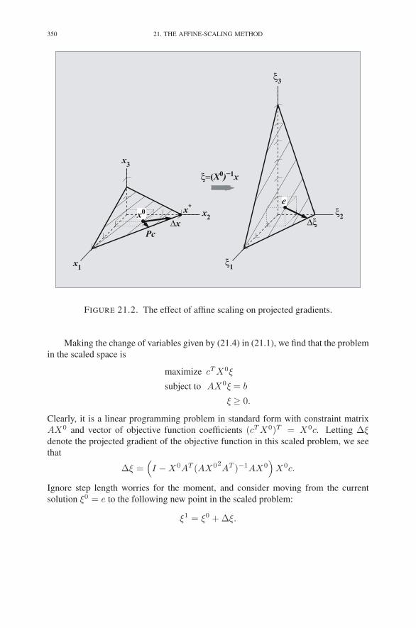
350 21. THE AFFINE-SCALING METHOD
∆x
x*
Pc
x1
x3
ξ1
x2
ξ2
ξ3
x0
e
∆ξ
ξ=(X0)−1x
FIGURE 21.2. The effect of affine scaling on projected gradients.
Making the change of variables given by (21.4) in (21.1), we find that the problem
in the scaled space is
maximize cT X0ξ
subject to AX0ξ = b
ξ ≥ 0.
Clearly, it is a linear programming problem in standard form with constraint matrix
AX0 and vector of objective function coefficients (cT X0)T = X0c. Letting ∆ξdenote the projected gradient of the objective function in this scaled problem, we see
that
∆ξ =(
I − X0AT (AX02AT )−1AX0
)
X0c.
Ignore step length worries for the moment, and consider moving from the current
solution ξ0 = e to the following new point in the scaled problem:
ξ1 = ξ0 + ∆ξ.
3. THE PROJECTED GRADIENT DIRECTION WITH SCALING 351
Then transforming this new point back into the original unscaled variables, we get a
new point x1 given by
x1 = X0ξ1 = X0(e + ∆ξ) = x0 + X0∆ξ.
Of course, the difference between x1 and x0 is the step direction in the original vari-
ables. Denoting this difference by ∆x, we see that
∆x = X0(
I − X0AT (AX02AT )−1AX0
)
X0c
=(
D − DAT (ADAT )−1AD)
c,(21.5)
where
D = X02.
The expression for ∆x given by (21.5) is called the affine-scaling step direction. Of
course, to construct the affine-scaling algorithm out of this formula for a step direc-
tion, one simply needs to choose step lengths in such a manner as to ensure “strict”
feasibility of each iterate.
We end this section by illustrating some of the calculations on the following trivial
example:
maximize 2x1 + 3x2 + 2x3
subject to x1 + x2 + 2x3 = 3
x1, x2, x3 ≥ 0.
This is precisely the problem shown in Figure 21.2. As in the figure, let us assume that
x0 =
⎡
⎢
⎢
⎣
13214
⎤
⎥
⎥
⎦
.

352 21. THE AFFINE-SCALING METHOD
For later comparison, we compute the projected gradient (without scaling):
Pc = c − AT (AAT )−1Ac
=
⎡
⎢
⎢
⎣
2
3
2
⎤
⎥
⎥
⎦
−
⎡
⎢
⎢
⎣
1
1
2
⎤
⎥
⎥
⎦
⎛
⎜
⎜
⎝
[
1 1 2]
⎡
⎢
⎢
⎣
1
1
2
⎤
⎥
⎥
⎦
⎞
⎟
⎟
⎠
−1
[
1 1 2]
⎡
⎢
⎢
⎣
2
3
2
⎤
⎥
⎥
⎦
=
⎡
⎢
⎢
⎣
2
3
2
⎤
⎥
⎥
⎦
−
⎡
⎢
⎢
⎣
1
1
2
⎤
⎥
⎥
⎦
9
6
=
⎡
⎢
⎢
⎣
1232
−1
⎤
⎥
⎥
⎦
.
Now, in the scaled coordinate system, the gradient of the objective function is
X0c =
⎡
⎢
⎢
⎣
132
14
⎤
⎥
⎥
⎦
⎡
⎢
⎢
⎣
2
3
2
⎤
⎥
⎥
⎦
=
⎡
⎢
⎢
⎣
29212
⎤
⎥
⎥
⎦
and the constraint matrix is given by
AX0 =[
1 1 2]
⎡
⎢
⎢
⎣
132
14
⎤
⎥
⎥
⎦
=[
1 32
12
]
.
Using these, we compute ∆ξ as follows:
∆ξ =
⎡
⎢
⎢
⎣
29212
⎤
⎥
⎥
⎦
−
⎡
⎢
⎢
⎣
13212
⎤
⎥
⎥
⎦
⎛
⎜
⎜
⎝
[
1 32
12
]
⎡
⎢
⎢
⎣
13212
⎤
⎥
⎥
⎦
⎞
⎟
⎟
⎠
−1
[
1 32
12
]
⎡
⎢
⎢
⎣
29212
⎤
⎥
⎥
⎦
=
⎡
⎢
⎢
⎣
29212
⎤
⎥
⎥
⎦
−
⎡
⎢
⎢
⎣
13212
⎤
⎥
⎥
⎦
2
79
=
⎡
⎢
⎢
⎣
− 47914
− 1114
⎤
⎥
⎥
⎦
.

4. CONVERGENCE 353
Finally, ∆x is obtained by the inverse scaling:
∆x = X0∆ξ
=
⎡
⎢
⎢
⎣
132
14
⎤
⎥
⎥
⎦
⎡
⎢
⎢
⎣
− 47914
− 1114
⎤
⎥
⎥
⎦
=
⎡
⎢
⎢
⎣
− 472728
− 1156
⎤
⎥
⎥
⎦
.
In the next section, we discuss the convergence properties of the affine-scaling algo-
rithm.
4. Convergence
In the previous section, we derived the affine-scaling step direction ∆x. To make
an algorithm, we need to introduce an associated step length. If the step were chosen
so that the new point were to lie exactly on the boundary of the feasible region, then
the multiplier for ∆x, which as usual we denote by θ, would be given by
θ =
(
maxj
{
−∆xj
xj
})−1
.
But as always, we need to shorten the step by introducing a parameter 0 < r < 1 and
setting
θ = r
(
maxj
{
−∆xj
xj
})−1
.
With this choice of θ, the iterations of the affine-scaling algorithm are defined by
x ← x + θ∆x.
It turns out that the analysis of the affine-scaling algorithm is more delicate than
the analysis of the path-following algorithm that we discussed in Chapter 18. Hence,
we simply state without proof the main results.
THEOREM 21.1.
(a) If the problem and its dual are nondegenerate, then for every r < 1, the
sequence generated by the algorithm converges to the optimal solution.
(b) For r ≤ 2/3, the sequence generated by the algorithm converges to an
optimal solution (regardless of degeneracy).
(c) There exists an example and an associated r < 1 for which the algorithm
converges to a nonoptimal solution.
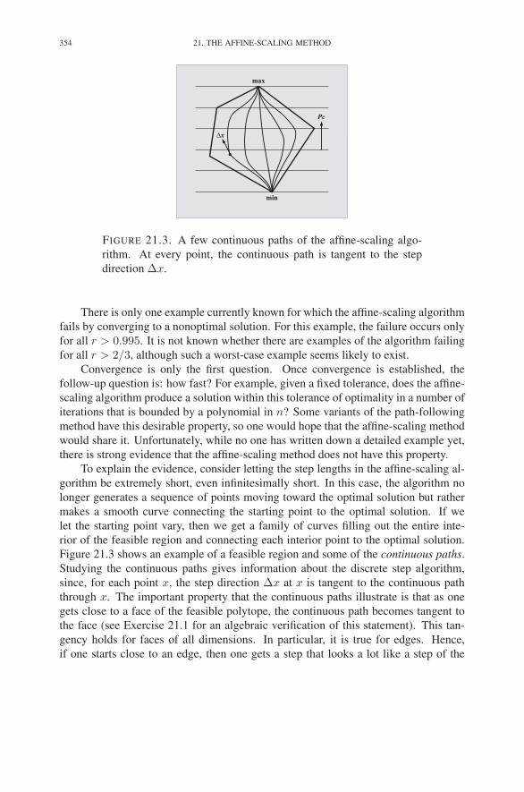
354 21. THE AFFINE-SCALING METHOD
Pc
min
max
∆x
FIGURE 21.3. A few continuous paths of the affine-scaling algo-
rithm. At every point, the continuous path is tangent to the step
direction ∆x.
There is only one example currently known for which the affine-scaling algorithm
fails by converging to a nonoptimal solution. For this example, the failure occurs only
for all r > 0.995. It is not known whether there are examples of the algorithm failing
for all r > 2/3, although such a worst-case example seems likely to exist.
Convergence is only the first question. Once convergence is established, the
follow-up question is: how fast? For example, given a fixed tolerance, does the affine-
scaling algorithm produce a solution within this tolerance of optimality in a number of
iterations that is bounded by a polynomial in n? Some variants of the path-following
method have this desirable property, so one would hope that the affine-scaling method
would share it. Unfortunately, while no one has written down a detailed example yet,
there is strong evidence that the affine-scaling method does not have this property.
To explain the evidence, consider letting the step lengths in the affine-scaling al-
gorithm be extremely short, even infinitesimally short. In this case, the algorithm no
longer generates a sequence of points moving toward the optimal solution but rather
makes a smooth curve connecting the starting point to the optimal solution. If we
let the starting point vary, then we get a family of curves filling out the entire inte-
rior of the feasible region and connecting each interior point to the optimal solution.
Figure 21.3 shows an example of a feasible region and some of the continuous paths.
Studying the continuous paths gives information about the discrete step algorithm,
since, for each point x, the step direction ∆x at x is tangent to the continuous path
through x. The important property that the continuous paths illustrate is that as one
gets close to a face of the feasible polytope, the continuous path becomes tangent to
the face (see Exercise 21.1 for an algebraic verification of this statement). This tan-
gency holds for faces of all dimensions. In particular, it is true for edges. Hence,
if one starts close to an edge, then one gets a step that looks a lot like a step of the
5. FEASIBILITY DIRECTION 355
simplex method. Therefore, it is felt that if one were to take a problem that is bad
for the simplex method, such as the Klee–Minty problem, and start the affine-scaling
algorithm in just the right place, then it would mimic the steps of the simplex method
and therefore take 2n iterations to get close to the optimal solution. This is the idea,
but as noted above, no one has carried out the calculations.
5. Feasibility Direction
To derive a Phase I procedure for the affine-scaling algorithm, we consider a start-
ing point x0 that has strictly positive components but does not necessarily satisfy the
equality constraints Ax = b. We then let
ρ = b − Ax0
denote the vector of infeasibilities. With these definitions under our belt, we introduce
the following auxiliary problem involving one extra variable, which we shall denote
by x0 (not to be confused with the initial solution vector x0):
maximize −x0
subject to Ax + x0ρ = b
x ≥ 0, x0 ≥ 0.
Clearly, the vector[
x0
1
]
is a strictly positive feasible solution to the auxiliary problem. Hence, we can apply the
affine-scaling algorithm to the auxiliary problem. If the optimal solution has x∗0 > 0,
then the original problem is infeasible. If, on the other hand, the optimal solution has
x∗0 = 0, then the optimal solution to the auxiliary problem provides a feasible starting
solution to the original problem (it may not be a strictly interior feasible solution, but
we shall ignore such technicalities in the present discussion).
Let us now derive a specific formula for the step direction vector in the auxiliary
problem. The vector of objective coefficients is[
0
−1
]
,
the constraint matrix is[
A ρ]
,
and the “current” solution can be denoted as[
x
x0
]
.
356 21. THE AFFINE-SCALING METHOD
Substituting these three objects appropriately into (21.5), we get[
∆x
∆x0
]
=
([
X2
x20
]
−[
X2
x20
][
AT
ρT
]
(
[
A ρ]
[
X2
x20
][
AT
ρT
])−1
[
A ρ]
[
X2
x20
])[
0
−1
]
.
Exploiting heavily the fact that all the coefficients in the objective vector are zero
except for the last, we can write a fairly simple expression for ∆x:
∆x = X2AT(
AX2AT + x20ρρT
)−1ρx0.
The final simplification comes from applying the Sherman–Morrison–Woodbury for-
mula (see Exercise 19.1) to the inverted expression above to discover that the vector
(AX2AT + x20ρρT )−1ρ points in the same direction as (AX2AT )−1ρ. That is, there
is a positive scalar α such that
(AX2AT + x20ρρT )−1ρ = α(AX2AT )−1ρ
(see Exercise 21.3). Since vector lengths are irrelevant, we can define the affine-
scaling feasibility step direction as
(21.6) ∆x = X2AT(
AX2AT)−1
ρ.
6. Problems in Standard Form
We return now to problems in standard form:
maximize cT x
subject to Ax≤ b
x≥ 0.
Introducing slack variables w, we can write the problem equivalently as
(21.7)
maximize
[
c
0
]T [
x
w
]
subject to[
A I]
[
x
w
]
= b
[
x
w
]
≥ 0.

EXERCISES 357
Writing down the affine-scaling step direction for this problem, we get[
∆x
∆w
]
=
([
X2
W 2
]
−[
X2
W 2
][
AT
I
]
(
[
A I]
[
X2
W 2
][
AT
I
])−1
[
A I]
[
X2
W 2
])[
c
0
]
,
which simplifies to[
∆x
∆w
]
=
[
X2c
0
]
−[
X2AT
W 2
]
(
AX2AT + W 2)−1
AX2c.
Therefore, in particular
∆x = X2c − X2AT (AX2AT + W 2)−1AX2c.
Note that this formula for ∆x matches the formula for ∆xOPT given in Section 19.3,
except that the diagonal matrix X2 replaces XZ−1 and W 2 replaces WY −1. These
diagonal matrices are referred to as scaling matrices. Hence, the formula for ∆x given
above is often called the affine-scaling step direction with primal scaling, whereas
∆xOPT is referred to as the affine-scaling step direction with primal–dual scaling.
Similar connections can be established between the Phase I step direction derived
in this section and ∆xFEAS from Section 19.3. Indeed, from (21.6), we see that the
feasibility step direction for (21.7) is[
∆x
∆w
]
=
[
X2
W 2
][
AT
I
](
[
A I]
[
X2
W 2
][
AT
I
])−1
(
b −[
A I]
[
x
w
])
.
Again, looking just at the formula for ∆x, we see that
∆x = X2AT (AX2AT + W 2)−1(b − Ax − w),
which coincides with ∆xFEAS except that X2 replaces XZ−1 and W 2 replaces WY −1.
Exercises
21.1 Step direction becomes tangent to each facet. Let ∆x denote the affine-
scaling step direction given by
∆x =(
X2 − X2AT (AX2AT )−1AX2)
c.

358 21. THE AFFINE-SCALING METHOD
This step direction is clearly a function of x. Fix j. Show that the limit as
xj tends to zero of ∆x is a vector whose jth component vanishes. That is,
limxj→0
∆xj = 0.
21.2 Dual Estimates. Consider the following function, defined in the interior of
the polytope of feasible solutions {x : Ax = b, x > 0} by
y(x) = (AX2AT )−1AX2c.
Consider a partition of the columns of A =[
B N]
into a basic part B and a
nonbasic part N , and, as we did in our study of the simplex method, partition
the n-vectors analogously. Show that
limxN→0
y(x) = (BT )−1cB.
21.3 Let A be an m×n matrix having rank m, and let ρ be an arbitrary m-vector.
Use the identity proved in Exercise 19.1 to show that there exists a scalar αsuch that
(AAT + ρρT )−1ρ = α(AAT )−1ρ.
Hint: Be mindful of which matrices are invertible.
21.4 (So-called) Dual Affine-Scaling Method. Compute the affine-scaling step-
direction vector ∆x for problems in the following form:
maximize cT x
subject to Ax ≤ b.
Notes
The affine-scaling algorithm was first suggested by Dikin (1967). He subse-
quently published a convergence analysis in Dikin (1974). Dikin’s work went largely
unnoticed for many years until several researchers independently rediscovered the
affine-scaling algorithm as a simple variant of Karmarkar’s algorithm (Karmarkar
1984). Of these independent rediscoveries, only two papers offered a convergence
analysis: one by Barnes (1986) and the other by Vanderbei et al. (1986). It is inter-
esting to note that Karmarkar himself was one of the independent rediscoverers, but
he mistakenly believed that the algorithm enjoyed the same convergence properties as
his algorithm (i.e., that it would get within any fixed tolerance of optimality within a
specific number of iterations bounded by a polynomial in n).
Theorem 21.1(a) was proved by Vanderbei et al. (1986). Part (b) of the theorem
was proved by Tsuchiya & Muramatsu (1992) who also show that the result is sharp.
A sharper sharpness result can be found in Hall & Vanderbei (1993). Part (c) of the
Theorem was established by Mascarenhas (1997).

NOTES 359
The first derivation of the affine-scaling feasibility step direction was given by
Vanderbei (1989). The simple derivation given in Section 21.5 is due to M. Meketon.
A recent book by Saigal (1995) contains an extensive treatment of affine-scaling
methods.

CHAPTER 22
The Homogeneous Self-Dual Method
In Chapter 18, we described and analyzed an interior-point method called the
path-following algorithm. This algorithm is essentially what one implements in prac-
tice but as we saw in the section on convergence analysis, it is not easy (and perhaps
not possible) to give a complete proof that the method converges to an optimal solu-
tion. If convergence were completely established, the question would still remain as
to how fast is the convergence. In this chapter, we shall present a similar algorithm for
which a complete convergence analysis can be given.
1. From Standard Form to Self-Dual Form
As always, we are interested in a linear programming problem given in standard
form
(22.1)
maximize cT x
subject to Ax≤ b
x≥ 0
and its dual
(22.2)
minimize bT y
subject to AT y ≥ c
y ≥ 0.
As we shall show, these two problems can be solved by solving the following problem,
which essentially combines the primal and dual problems into one problem:
(22.3)
maximize 0
subject to − AT y + cφ ≤ 0,
Ax − bφ ≤ 0,
−cT x + bT y ≤ 0,
x, y, φ ≥ 0.
Note that, beyond combining the primal and dual into one big problem, one new vari-
able (φ) and one new constraint have been added. Hence, the total number of variables
361
362 22. THE HOMOGENEOUS SELF-DUAL METHOD
in (22.3) is n + m + 1 and the total number of constraints is n + m + 1. Furthermore,
the objective function and the right-hand sides all vanish. Problems with such right-
hand sides are called homogeneous. Also, the constraint matrix for problem (22.3) is
skew symmetric. That is, it is equal to the negative of its transpose. Homogeneous
linear programming problems having a skew symmetric constraint matrix are called
self-dual.
In the next section, we shall give an algorithm for the solution of homogeneous
self-dual linear programming problems. But first, let’s note that a solution to (22.3) in
which φ > 0 can be converted into solutions for (22.1) and (22.2). Indeed, let (x, y, φ)be an optimal solution to problem (22.3). Suppose that φ > 0. (The algorithm given
in the next section will guarantee that this property is satisfied whenever (22.1) and
(22.2) have optimal solutions1). Put
x∗ = x/φ and y∗ = y/φ.
Then the constraints in (22.3) say that
− AT y∗ + c ≤ 0,
Ax∗ − b ≤ 0,
−cT x∗ + bT y∗ ≤ 0.
Also, x∗ and y∗ are both nonnegative. Therefore, x∗ is feasible for (22.1) and y∗ is
feasible for (22.2). From the weak duality theorem together with the third inequality
above, we get
cT x∗ = bT y∗.
Therefore, x∗ is optimal for the primal problem (22.1) and y∗ is optimal for the dual
problem (22.2). As we will see later, the case where φ = 0 corresponds to infeasibility
of either the primal or the dual problem (or both).
2. Homogeneous Self-Dual Problems
Consider a linear programming problem in standard form
maximize cT x
subject to Ax≤ b
x≥ 0
and its dual
minimize bT y
subject to AT y ≥ c
y ≥ 0.
1The astute reader might notice that setting all variables to 0 produces an optimal solution.
2. HOMOGENEOUS SELF-DUAL PROBLEMS 363
Such a linear programming problem is called self-dual if m = n, A = −AT , and
b = −c. The reason for the name is that the dual of such a problem is the same as
the primal. To see this, rewrite the constraints as less-thans and then use the defining
properties for self-duality to get
AT y ≥ c ⇔ −AT y ≤ −c ⇔ Ay ≤ b.
Similarly, writing the objective function as a maximization, we get
min bT y = −max−bT y = −max cT y.
Hence, ignoring the (irrelevant) fact that the dual records the negative of the objective
function, the primal and the dual are seen to be the same. A linear programming
problem in which the right-hand side vanishes is called a homogeneous problem. It
follows that if a problem is homogeneous and self-dual, then its objective function
must vanish too.
For the remainder of this section, we assume that the problem under consideration
is homogeneous and self-dual. Since the case m = n = 1 is trivial (A = 0 in this
case), we assume throughout this section that n ≥ 2. Also, since the dual is the same
problem as the primal, we prefer to use the letter z for the primal slacks (instead of the
usual w). Hence, the primal can be written as
(22.4)
maximize 0
subject to Ax + z = 0
x, z ≥ 0.
The following theorem establishes some of the important properties of homoge-
neous self-dual problems.
THEOREM 22.1. For homogeneous self-dual problem (22.4), the following state-
ments hold:
(1) It has feasible solutions and every feasible solution is optimal.
(2) The set of feasible solutions has empty interior. In fact, if (x, z) is feasible,
then zT x = 0.
PROOF. (1) The trivial solution, (x, z) = (0, 0), is feasible. Since the objective
function is zero, every feasible solution is optimal.
(2) Suppose that (x, z) is feasible for (22.4). The fact that A is skew symmetric
implies that ξT Aξ = 0 for every vector ξ (see Exercise 16.1). In particular, xT Ax = 0.
Therefore, multiplying Ax+z = 0 on the left by xT , we get 0 = xT Ax+xT z = xT z.
This completes the proof. �
Part (2) of the previous theorem tells us that homogeneous self-dual problems do
not have central paths.

364 22. THE HOMOGENEOUS SELF-DUAL METHOD
2.1. Step Directions. As usual, the interior-point method we shall derive will
have the property that the intermediate solutions it produces will be infeasible. Hence,
let
ρ(x, z) = Ax + z
denote the infeasibility of a solution (x, z). Also, let
μ(x, z) =1
nxT z.
The number μ(x, z) measures the degree of noncomplementarity between x and z.
When x and z are clear from context, we shall simply write ρ for ρ(x, z) and μ for
μ(x, z).Step directions (∆x,∆z) are chosen to reduce the infeasibility and noncomple-
mentarity of the current solution by a given factor δ, 0 ≤ δ ≤ 1. Hence, we consider
the nonlinear system that would make the infeasibility and noncomplementarity of
(x + ∆x, z + ∆z) be δ times that of (x, z):
A(x + ∆x) + (z + ∆z) = δ(Ax + z),
(X + ∆X)(Z + ∆Z)e = δμ(x, z)e.
As usual, this system is nonlinear in the “delta” variables. Dropping the nonlinear
term (appearing only in the second equation), we get the following linear system of
equations for the step directions:
A∆x + ∆z =−(1 − δ)ρ(x, z),(22.5)
Z∆x + X∆z = δμ(x, z)e − XZe.(22.6)
With these step directions, we pick a step length θ and step to a new point:
x = x + θ∆x, z = z + θ∆z.
We denote the new ρ-vector by ρ and the new μ-value by μ:
ρ = ρ(x, z) and μ = μ(x, z).
The following theorem establishes some of the properties of these step directions.
THEOREM 22.2. The following relations hold:
(1) ∆zT ∆x = 0.
(2) ρ = (1 − θ + θδ)ρ.
(3) μ = (1 − θ + θδ)μ.
(4) XZe − μe = (1 − θ)(XZe − μe) + θ2∆X∆Ze.
PROOF. (1) We start by multiplying both sides of (22.5) on the left by ∆xT :
(22.7) ∆xT A∆x + ∆xT ∆z = −(1 − δ)∆xT ρ.
The skew symmetry of A (i.e., A = −AT ) implies that ∆xT A∆x = 0 (see Exercise
16.1). Hence, the left-hand side of (22.7) simplifies nicely:
∆xT A∆x + ∆xT ∆z = ∆xT ∆z.
2. HOMOGENEOUS SELF-DUAL PROBLEMS 365
Substituting the definition of ρ into the right-hand side of (22.7), we get
−(1 − δ)∆xT ρ = −(1 − δ)∆xT (Ax + z).
Next, we use the skew symmetry of A to rewrite ∆xT Ax as follows:
∆xT Ax = (Ax)T ∆x = xT AT ∆x = −xT A∆x.
Assembling what we have so far, we see that
(22.8) ∆xT ∆z = −(1 − δ)(−xT A∆x + zT ∆x).
To proceed, we use (22.5) to replace A∆x with −(1 − δ)ρ − ∆z. Therefore,
− xT A∆x + zT ∆x = xT ((1 − δ)ρ + ∆z) + zT ∆x
= (1 − δ)xT ρ + xT ∆z + zT ∆x.(22.9)
Again using the definition of ρ and the skew symmetry of A, we see that
xT ρ = xT (Ax + z) = xT z.
The last two terms in (22.9) can be simplified by multiplying both sides of (22.6) on
the left by eT and then using the definition of μ to see that
zT ∆x + xT ∆z = δμn − xT z = (δ − 1)xT z..
Making these substitutions in (22.9), we get
−xT A∆x + zT ∆x = (1 − δ)xT z + (δ − 1)xT z = 0.
Hence, from (22.8), we see that ∆xT ∆z vanishes as claimed.
(2) From the definitions of x and z, we see that
ρ = A(x + θ∆x) + (z + θ∆z)
= Ax + z + θ(A∆x + ∆z)
= (1 − θ + θδ)ρ.
(3) From the definitions of x and z, we see that
xT z = (x + θ∆x)T (z + θ∆z)
= xT z + θ(zT ∆x + xT ∆z) + θ2∆zT ∆x.
From part (1) and (22.6), we then get
xT z = xT z + θ(δμn − xT z).
Therefore,
μ =1
nxT z = (1 − θ)μ + θδμ.
(4) From the definitions of x and z together with part (3), we see that
XZe − μe = (X + θ∆X)(Z + θ∆Z)e − (1 − θ + θδ)μe
= XZe + θ(Z∆x + X∆z) + θ2∆X∆Ze − (1 − θ + θδ)μe.

366 22. THE HOMOGENEOUS SELF-DUAL METHOD
Substituting (22.6) into the second term on the right and recollecting terms, we get the
desired expression. �
2.2. Predictor-Corrector Algorithm. With the preliminaries behind us, we are
now ready to describe an algorithm. We shall be more conservative than we were in
Chapter 18 and define the algorithm in such a way that it keeps the components of
XZe close to each other. Indeed, for each 0 ≤ β ≤ 1, let
N (β) = {(x, z) > 0 : ‖XZe − μ(x, z)e‖ ≤ βμ(x, z)} .
Shortly, we will only deal with N (1/4) and N (1/2) but first let us note generally that
β < β′ implies that N (β) ⊂ N (β′). Hence, as a function of β, the N (β)’s form an
increasing family of sets. Also, N (0) is precisely the set of points (x, z) for which
XZe has all equal components.
The algorithm alternates between two types of steps. On the first iteration and
subsequently on every other iteration, the algorithm performs a predictor step. Before
a predictor step, one assumes that
(x, z) ∈ N (1/4).
Then step directions are computed using δ = 0 (i.e., with no centering) and the step
length is calculated so as not to go outside of N (1/2):
(22.10) θ = max{t : (x + t∆x, z + t∆z) ∈ N (1/2)}.
On the even iterations, the algorithm performs a corrector step. Before a corrector
step, one assumes that
(x, z) ∈ N (1/2)
(as is guaranteed by the predictor step’s step length). Then step directions are com-
puted using δ = 1 (i.e., pure centering) and the step length parameter θ is set to 1.
The following theorem shows that the result of each step satisfies the precondition
for the next step of the algorithm and that μ decreases on predictor steps while it stays
the same on corrector steps.
THEOREM 22.3. The following statements are true:
(1) After a predictor step, (x, z) ∈ N (1/2) and μ = (1 − θ)μ.
(2) After a corrector step, (x, z) ∈ N (1/4) and μ = μ.
PROOF OF PART (1). The formula for μ follows from part (3) of Theorem 22.2
by putting δ = 0. The fact that (x, z) ∈ N (1/2) is an immediate consequence of the
choice of θ. �
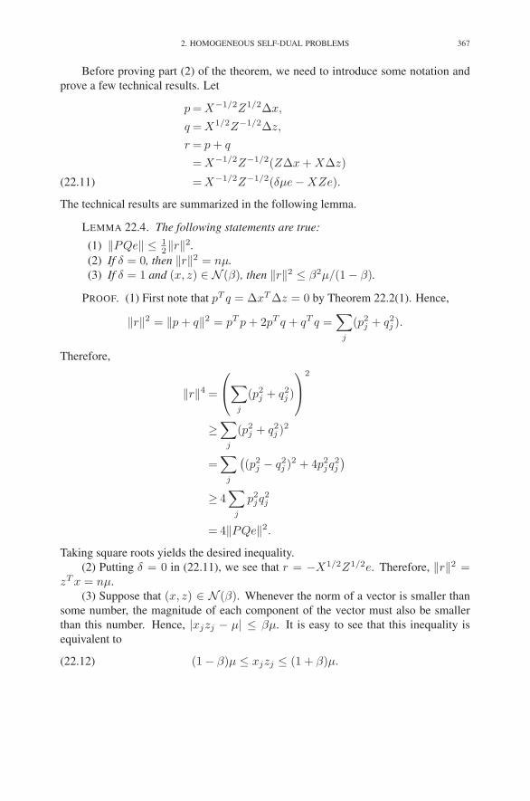
2. HOMOGENEOUS SELF-DUAL PROBLEMS 367
Before proving part (2) of the theorem, we need to introduce some notation and
prove a few technical results. Let
p = X−1/2Z1/2∆x,
q = X1/2Z−1/2∆z,
r = p + q
= X−1/2Z−1/2(Z∆x + X∆z)
= X−1/2Z−1/2(δμe − XZe).(22.11)
The technical results are summarized in the following lemma.
LEMMA 22.4. The following statements are true:
(1) ‖PQe‖ ≤ 12‖r‖2.
(2) If δ = 0, then ‖r‖2 = nμ.
(3) If δ = 1 and (x, z) ∈ N (β), then ‖r‖2 ≤ β2μ/(1 − β).
PROOF. (1) First note that pT q = ∆xT ∆z = 0 by Theorem 22.2(1). Hence,
‖r‖2 = ‖p + q‖2 = pT p + 2pT q + qT q =∑
j
(p2j + q2
j ).
Therefore,
‖r‖4 =
⎛
⎝
∑
j
(p2j + q2
j )
⎞
⎠
2
≥∑
j
(p2j + q2
j )2
=∑
j
(
(p2j − q2
j )2 + 4p2jq
2j
)
≥ 4∑
j
p2jq
2j
= 4‖PQe‖2.
Taking square roots yields the desired inequality.
(2) Putting δ = 0 in (22.11), we see that r = −X1/2Z1/2e. Therefore, ‖r‖2 =zT x = nμ.
(3) Suppose that (x, z) ∈ N (β). Whenever the norm of a vector is smaller than
some number, the magnitude of each component of the vector must also be smaller
than this number. Hence, |xjzj − μ| ≤ βμ. It is easy to see that this inequality is
equivalent to
(22.12) (1 − β)μ ≤ xjzj ≤ (1 + β)μ.

368 22. THE HOMOGENEOUS SELF-DUAL METHOD
Now putting δ = 1 in (22.11), we get
‖r‖2 =∑
j
(xjzj − μ)2
xjzj.
Therefore, using the lower bound given in (22.12), we get the following upper bound:
‖r‖2 ≤ 1
(1 − β)μ
∑
j
(xjzj − μ)2.
Finally, since (x, z) ∈ N (β), we see that the above sum is bounded by β2μ2. This
gives the claimed inequality. �
PROOF OF THEOREM 22.3(2). Since θ = 1 in a corrector step, it follows from
Theorem 22.2(4) that XZe − μe = ∆X∆Ze = PQe. Therefore, parts (1) and (3) of
Lemma 22.4 imply that
‖XZe − μe‖= ‖PQe‖
≤ 1
2‖r‖2
≤ 1
2
(1/2)2
1 − 1/2μ
=1
4μ.(22.13)
We also need to show that (x, z) > 0. For 0 ≤ t ≤ 1, let
x(t) = x + t∆x, z(t) = z + t∆z, and μ(t) = μ(x(t), z(t)).
Then from part (4) of Theorem 22.2, we have
X(t)Z(t)e − μ(t)e = (1 − t)(XZe − μe) + t2∆X∆Ze.
The right-hand side is the sum of two vectors. Since the length of the sum of two
vectors is less than the sum of the lengths (i.e., by the triangle inequality), it follows
that
(22.14) ‖X(t)Z(t)e − μ(t)e‖ ≤ (1 − t)‖XZe − μe‖ + t2‖∆X∆Ze‖(note that we’ve pulled the scalars out of the norms). Now, since (x, z) ∈ N (1/2),we have ‖XZe−μe‖ ≤ μ/2. Furthermore, from (22.13) we have that ‖∆X∆Ze‖ =‖PQe‖ ≤ μ/4. Replacing the norms in (22.14) with these upper bounds, we get the
following bound:
(22.15) ‖X(t)Z(t)e − μ(t)e‖ ≤ (1 − t)μ
2+ t2
μ
4≤ μ
2
(the second inequality follows from the obvious facts that t2 ≤ t and μ/4 ≤ μ/2).
Now, consider a specific component j. It follows from (22.15) that
xj(t)zj(t) − μ(t) ≥ −μ
2.

2. HOMOGENEOUS SELF-DUAL PROBLEMS 369
Since δ = 1, part (3) of Theorem 22.2 tells us that μ(t) = μ for all t. Therefore the
previous inequality can be written as
(22.16) xj(t)zj(t) ≥μ
2> 0.
This inequality then implies that xj(t) > 0 and zj(t) > 0 for all 0 ≤ t ≤ 1 (since
they could only become negative by passing through 0, which is ruled out by (22.16)).
Putting t = 1, we get that xj > 0 and zj > 0. Since the component j was arbitrary, it
follows that (x, z) > 0. Therefore (x, z) ∈ N (1/4). �
2.3. Convergence Analysis. The previous theorem showed that the predictor-
corrector algorithm is well defined. The next theorem gives us a lower bound on the
progress made by each predictor step.
THEOREM 22.5. In each predictor step, θ ≥ 12√
n.
PROOF. Using the same notation as in the proof of Theorem 22.3, we have the
inequality:
‖X(t)Z(t)e − μ(t)e‖ ≤ (1 − t)‖XZe − μe‖(22.17)
+t2‖∆X∆Ze‖.This time, however, (x, z) ∈ N (1/4) and δ = 0. Hence,
‖XZe − μe‖ ≤ μ
4
and, from parts (1) and (2) of Lemma 22.4,
‖∆X∆Ze‖ = ‖PQe‖ ≤ 1
2‖r‖2 =
1
2nμ.
Using these two bounds in (22.17), we get the following bound:
‖X(t)Z(t)e − μ(t)e‖ ≤ (1 − t)μ
4+ t2
nμ
2.
Now, fix a t ≤ (2√
n)−1. For such a t, we have t2n/2 ≤ 1/8. Therefore, using the
fact that t ≤ 1/2 for n ≥ 2, we get
‖X(t)Z(t)e − μ(t)e‖ ≤ (1 − t)μ
4+
μ
8
≤ (1 − t)μ
4+ (1 − t)
μ
4
= (1 − t)μ
2
=μ(t)
2.
Hence, as in the previous theorem, (x(t), z(t)) ∈ N (1/2). Since t was an arbitrary
number less than (2√
n)−1, it follows that θ ≥ (2√
n)−1. �
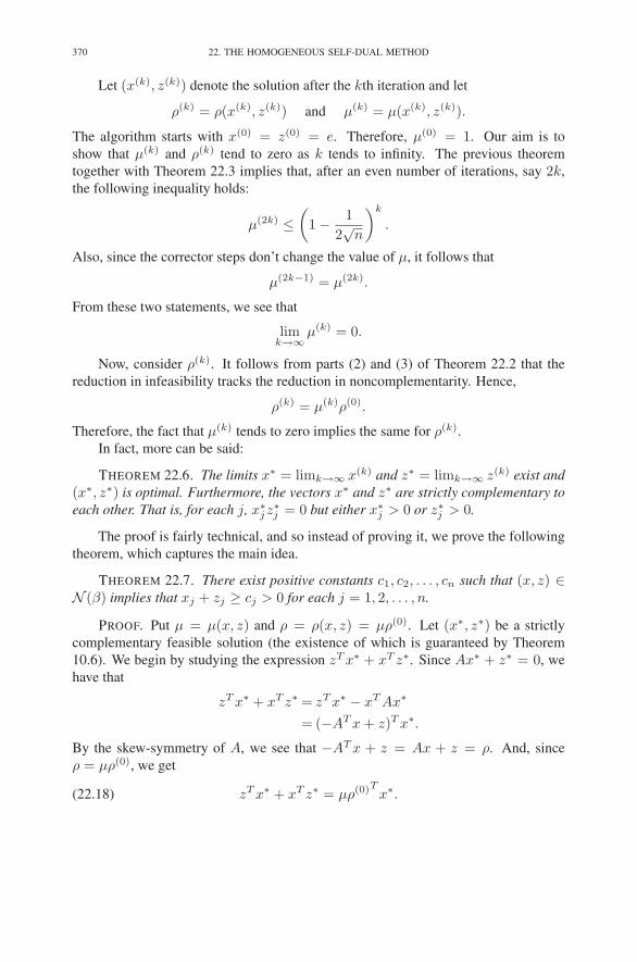
370 22. THE HOMOGENEOUS SELF-DUAL METHOD
Let (x(k), z(k)) denote the solution after the kth iteration and let
ρ(k) = ρ(x(k), z(k)) and μ(k) = μ(x(k), z(k)).
The algorithm starts with x(0) = z(0) = e. Therefore, μ(0) = 1. Our aim is to
show that μ(k) and ρ(k) tend to zero as k tends to infinity. The previous theorem
together with Theorem 22.3 implies that, after an even number of iterations, say 2k,
the following inequality holds:
μ(2k) ≤(
1 − 1
2√
n
)k
.
Also, since the corrector steps don’t change the value of μ, it follows that
μ(2k−1) = μ(2k).
From these two statements, we see that
limk→∞
μ(k) = 0.
Now, consider ρ(k). It follows from parts (2) and (3) of Theorem 22.2 that the
reduction in infeasibility tracks the reduction in noncomplementarity. Hence,
ρ(k) = μ(k)ρ(0).
Therefore, the fact that μ(k) tends to zero implies the same for ρ(k).
In fact, more can be said:
THEOREM 22.6. The limits x∗ = limk→∞ x(k) and z∗ = limk→∞ z(k) exist and
(x∗, z∗) is optimal. Furthermore, the vectors x∗ and z∗ are strictly complementary to
each other. That is, for each j, x∗jz
∗j = 0 but either x∗
j > 0 or z∗j > 0.
The proof is fairly technical, and so instead of proving it, we prove the following
theorem, which captures the main idea.
THEOREM 22.7. There exist positive constants c1, c2, . . . , cn such that (x, z) ∈N (β) implies that xj + zj ≥ cj > 0 for each j = 1, 2, . . . , n.
PROOF. Put μ = μ(x, z) and ρ = ρ(x, z) = μρ(0). Let (x∗, z∗) be a strictly
complementary feasible solution (the existence of which is guaranteed by Theorem
10.6). We begin by studying the expression zT x∗ + xT z∗. Since Ax∗ + z∗ = 0, we
have that
zT x∗ + xT z∗ = zT x∗ − xT Ax∗
= (−AT x + z)T x∗.
By the skew-symmetry of A, we see that −AT x + z = Ax + z = ρ. And, since
ρ = μρ(0), we get
(22.18) zT x∗ + xT z∗ = μρ(0)Tx∗.
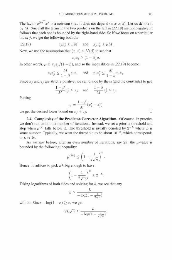
2. HOMOGENEOUS SELF-DUAL PROBLEMS 371
The factor ρ(0)Tx∗ is a constant (i.e., it does not depend on x or z). Let us denote it
by M . Since all the terms in the two products on the left in (22.18) are nonnegative, it
follows that each one is bounded by the right-hand side. So if we focus on a particular
index j, we get the following bounds:
(22.19) zjx∗j ≤ μM and xjz
∗j ≤ μM.
Now, we use the assumption that (x, z) ∈ N (β) to see that
xjzj ≥ (1 − β)μ.
In other words, μ ≤ xjzj/(1 − β), and so the inequalities in (22.19) become
zjx∗j ≤ M
1 − βzjxj and xjz
∗j ≤ M
1 − βxjzj .
Since xj and zj are strictly positive, we can divide by them (and the constants) to get
1 − β
Mx∗
j ≤ xj and1 − β
Mz∗j ≤ zj .
Putting
cj =1 − β
M(x∗
j + z∗j ),
we get the desired lower bound on xj + zj . �
2.4. Complexity of the Predictor-Corrector Algorithm. Of course, in practice
we don’t run an infinite number of iterations. Instead, we set a priori a threshold and
stop when μ(k) falls below it. The threshold is usually denoted by 2−L where L is
some number. Typically, we want the threshold to be about 10−8, which corresponds
to L ≈ 26.
As we saw before, after an even number of iterations, say 2k, the μ-value is
bounded by the following inequality:
μ(2k) ≤(
1 − 1
2√
n
)k
.
Hence, it suffices to pick a k big enough to have(
1 − 1
2√
n
)k
≤ 2−L.
Taking logarithms of both sides and solving for k, we see that any
k ≥ L
− log(1 − 12√
n)
will do. Since − log(1 − x) ≥ x, we get
2L√
n ≥ L
− log(1 − 12√
n).

372 22. THE HOMOGENEOUS SELF-DUAL METHOD
Therefore, any k ≥ 2L√
n will do. In particular, k = 2L√
n rounded up to the nearest
integer will suffice. Since k represents half the number of iterations, it follows that it
will take at most 4L√
n iterations for the μ-value to fall below the threshold of 2−L.
This bound implies that the method is a polynomial algorithm, since it says that any
desired precision can be obtained in a number of iterations that is bounded above by a
polynomial in n (here, 4L√
n is not itself a polynomial but is bounded above by say a
linear function in n for n ≥ 2).
2.5. The KKT System. We end this section on homogeneous self-dual problems
by briefly discussing the KKT system (22.5)–(22.6). Solving this system of equations
is the most time consuming step within each iteration of the predictor-corrector al-
gorithm. There are several ways in which one can organize the computation. The
approach that most parallels what we have done before is first to solve (22.6) for ∆z,
∆z = X−1(−Z∆x + δμe − XZe)(22.20)
=−X−1Z∆x + δμX−1e − z,
and then to eliminate it from (22.5) to get the following reduced KKT system:
(A − X−1Z)∆x = −(1 − δ)ρ + z − δμX−1e.
In the next section, we apply the algorithm developed in this section to the homoge-
neous self-dual problem given by (22.3).
3. Back to Standard Form
We return now to the setup in Section 1. Let z, w, and ψ denote the slack variables
for the constraints in problem (22.3):
(22.21)
maximize 0
subject to − AT y + cφ + z = 0,
Ax − bφ + w = 0,
−cT x + bT y + ψ = 0,
x, y, φ, z, w, ψ ≥ 0.
We say that a feasible solution (x, y, φ, z, w, ψ) is strictly complementary if xj + zj >0 for all j, yi + wi > 0 for all i, and φ + ψ > 0. Theorem 10.6 ensures the existence
of such a solution (why?).
The following theorem summarizes and extends the motivating discussion given
in Section 1.
THEOREM 22.8. Suppose that (x, y, φ, z, w, ψ) is a strictly complementary fea-
sible (hence, optimal) solution to (22.21).
(1) If φ > 0, then x∗ = x/φ is optimal for the primal problem (22.1) and
y∗ = y/φ is optimal for its dual (22.2).

3. BACK TO STANDARD FORM 373
(2) If φ = 0, then either cT x > 0 or bT y < 0.
(a) If cT x > 0, then the dual problem is infeasible.
(b) If bT y < 0, then the primal problem is infeasible.
PROOF. Part (1) was proved in Section 1. For part (2), suppose that φ = 0. By
strict complementarity, ψ > 0. Hence, x and y satisfy
AT y ≥ 0,
Ax≤ 0,(22.22)
bT y < cT x.
From the last inequality, we see that it is impossible to have bT y ≥ 0 and cT x ≤ 0.
That is, either cT x > 0 or bT y < 0 (or both). Suppose, without loss of generality, that
cT x > 0. We will prove by contradiction that the dual problem is infeasible. To this
end, suppose that there exists a vector y0 ≥ 0 such that
(22.23) AT y0 ≥ c.
Since x ≥ 0, we can multiply by it without changing the direction of an inequality. So
multiplying (22.23) on the left by xT , we get
xT AT y0 ≥ xT c.
Now, the right-hand side is strictly positive. But inequality (22.22) together with the
nonnegativity of y0 implies that the left-hand side is nonpositive:
xT AT y0 = (Ax)T y0 ≤ 0.
This is a contradiction and therefore the dual must be infeasible. �
3.1. The Reduced KKT System. The right-hand side in the reduced KKT sys-
tem involves the vector of infeasibilities. We partition this vector into three parts as
follows:⎡
⎢
⎢
⎣
σ
ρ
γ
⎤
⎥
⎥
⎦
=
⎡
⎢
⎢
⎣
−AT c
A −b
−cT bT
⎤
⎥
⎥
⎦
⎡
⎢
⎢
⎣
x
y
φ
⎤
⎥
⎥
⎦
+
⎡
⎢
⎢
⎣
z
w
ψ
⎤
⎥
⎥
⎦
=
⎡
⎢
⎢
⎣
−AT y + cφ + z
Ax − bφ + w
−cT x + bT y + φ
⎤
⎥
⎥
⎦
.
The reduced KKT system for (22.3) is given by
(22.24)
⎡
⎢
⎢
⎣
−X−1Z −AT c
A −Y −1W −b
−cT bT −ψ/φ
⎤
⎥
⎥
⎦
⎡
⎢
⎢
⎣
∆x
∆y
∆φ
⎤
⎥
⎥
⎦
=
⎡
⎢
⎢
⎣
σ
ρ
γ
⎤
⎥
⎥
⎦
,
where⎡
⎢
⎢
⎣
σ
ρ
γ
⎤
⎥
⎥
⎦
=
⎡
⎢
⎢
⎣
−(1 − δ)σ + z − δμX−1e
−(1 − δ)ρ + w − δμY −1e
−(1 − δ)γ + ψ − δμ/φ
⎤
⎥
⎥
⎦
.
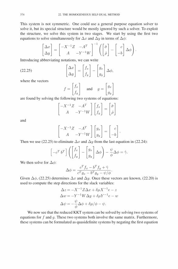
374 22. THE HOMOGENEOUS SELF-DUAL METHOD
This system is not symmetric. One could use a general purpose equation solver to
solve it, but its special structure would be mostly ignored by such a solver. To exploit
the structure, we solve this system in two stages. We start by using the first two
equations to solve simultaneously for ∆x and ∆y in terms of ∆φ:[
∆x
∆y
]
=
[
−X−1Z −AT
A −Y −1W
]−1 ([
σ
ρ
]
−[
c
−b
]
∆φ
)
.
Introducing abbreviating notations, we can write
(22.25)
[
∆x
∆y
]
=
[
fx
fy
]
−[
gx
gy
]
∆φ,
where the vectors
f =
[
fx
fy
]
and g =
[
gx
gy
]
are found by solving the following two systems of equations:[
−X−1Z −AT
A −Y −1W
][
fx
fy
]
=
[
σ
ρ
]
and[
−X−1Z −AT
A −Y −1W
][
gx
gy
]
=
[
c
−b
]
.
Then we use (22.25) to eliminate ∆x and ∆y from the last equation in (22.24):
[
−cT bT]
([
fx
fy
]
−[
gx
gy
]
∆φ
)
− ψ
φ∆φ = γ.
We then solve for ∆φ:
∆φ =cT fx − bT fy + γ
cT gx − bT gy − ψ/φ.
Given ∆φ, (22.25) determines ∆x and ∆y. Once these vectors are known, (22.20) is
used to compute the step directions for the slack variables:
∆z =−X−1Z∆x + δμX−1e − z
∆w =−Y −1W∆y + δμY −1e − w
∆ψ =−ψ
φ∆φ + δμ/φ − ψ.
We now see that the reduced KKT system can be solved by solving two systems of
equations for f and g. These two systems both involve the same matrix. Furthermore,
these systems can be formulated as quasidefinite systems by negating the first equation

4. SIMPLEX METHOD VS INTERIOR-POINT METHODS 375
and then reordering the equations appropriately. For example, the quasidefinite system
for g is[
−Y −1W A
AT X−1Z
][
gy
gx
]
=
[
−b
−c
]
.
Therefore, the techniques developed in Chapter 20 can be used to solve these systems
of equations. In particular, to solve the two systems, the quasidefinite matrix only
needs to be factored once. Then the two systems can be solved by doing two forward
and two backward substitutions. Since factorization requires more computation than
forward and backward substitutions, one would expect to be able to solve these two
systems in much less time than if they were each being solved from scratch. In fact,
it is often the case that one can solve two systems involving the same quasidefinite
matrix in little more time than is required to solve just one such system.
The full homogeneous self-dual method is summarized in Figure 22.1.
4. Simplex Method vs Interior-Point Methods
Finally, we compare the performance of interior-point methods with the simplex
method. For this comparison, we have chosen the homogeneous self-dual method
described in this chapter and the self-dual simplex method (see Figure 7.1). In the
interest of efficiency certain liberties have been taken with the implementations. For
example, in the homogeneous self-dual method, (18.6) is used to compute “long” step
lengths instead of the more conservative “short” step lengths in (22.10). The code
fragments implementing each of these two algorithms are shown in Appendix A.
A standard collection of test problems, the so-called NETLIB suite, were used in
the comparison. Problems in this collection are formulated with bounds and ranges:
minimize cT x
subject to b ≤ Ax ≤ b + r
l ≤ x ≤ u.
However, to keep the algorithms as simple as possible, they were implemented only for
problems in our standard inequality form. Therefore, the problems from the NETLIB
suite were converted to standard form as follows:
− maximize −cT x − cT l
subject to −Ax ≤ −b + Al
Ax ≤ b + r − Al
x ≤ u − l
x ≥ 0.

376 22. THE HOMOGENEOUS SELF-DUAL METHOD
initialize
(x, y, φ, z, w, ψ) = (e, e, 1, e, e, 1)
while (not optimal) {
µ = (zT x + wT y + ψφ)/(n + m + 1)
δ =
{
0, on odd iterations
1, on even iterations
ρ = −(1 − δ)(Ax − bφ + w) + w − δµY −1e
σ = −(1 − δ)(−AT y + cφ + z) + z − δµX−1e
γ = −(1 − δ)(bT y − cT x + ψ) + ψ − δµ/φ
solve the two (n + m) × (n + m) quasidefinite systems:[
−Y −1W A
AT X−1Z
] [
fy
fx
]
=
[
ρ
−σ
]
and[
−Y −1W A
AT X−1Z
] [
gy
gx
]
=
[
−b
−c
]
∆φ =cT fx − bT fy + γ
cT gx − bT gy − ψ/φ
[
∆x
∆y
]
=
[
fx
fy
]
−
[
gx
gy
]
∆φ
∆z = −X−1Z∆x + δµX−1e − z
∆w = −Y −1W∆y + δµY −1e − w
∆ψ = −ψ
φ∆φ + δµ/φ − ψ
θ =
{
max{t : (x(t), . . . , ψ(t)) ∈ N (1/2)}, on odd iterations
1, on even iterationsx ← x + θ∆x, z ← z + θ∆z
y ← y + θ∆y, w ← w + θ∆w
φ ← φ + θ∆φ, ψ ← ψ + θ∆ψ
}
FIGURE 22.1. The Homogeneous Self-Dual Method.
Of course, this transformation is invalid when any of the lower bounds are infinite.
Therefore, such problems have been dropped in our experiment. Also, this trans-
formation introduces significant computational inefficiency but, since it was applied
equally to the problems presented to both methods, the comparison remains valid.

4. SIMPLEX METHOD VS INTERIOR-POINT METHODS 377
The results of our experiment are shown in Table 22.1. The most obvious obser-
vation is that the simplex method is generally faster and that, for many problems, the
slower method is not more than 3 or 4 times slower. For problems in this suite, these
results are consistent with results reported in the literature. However, it must be noted
that the problems in this suite range only from small to medium in size. The largest
problem, fit2p, has about 3000 constraints and about 14000 variables. By today’s
standards, this problem is considered of medium size. For larger problems, reports
in the literature indicate that interior point methods tend to be superior although the
results are very much dependent on the specific class of problems. In the remaining
chapters of this book we shall consider various extensions of the linear programming
model. We shall see that the simplex method is particularly well suited for solving
integer programming problems studied in Chapter 23 whereas interior point methods
are more appropriate for extensions into the quadratic and convex programming prob-
lems studied in Chapters 24 and 25. These considerations are often more important
than speed. There are, of course, exceptions. For example, the interior-point method
is about 900 times faster than the simplex method on problem fit2p. Such a difference
cannot be ignored.
When comparing algorithms it is always tempting to look for ways to improve
the slower method. There are obvious enhancements to the interior-point method used
in this implementation. For example, one could use the same LDLT factorization to
compute both the predictor and the corrector directions. When implemented properly,
this enhancement alone can almost halve the times for this method.
Of course, the winning algorithm can also be improved (but, significant overall
improvements such as the one just mentioned for the interior-point method are not at
all obvious). Looking at the table, we note that the interior-point method solved both
fit2p and fit2d in roughly the same amount of time. These two problems are duals of
each other and hence any algorithm that treats the primal and the dual symmetrically
should take about the same time to solve them. Now, look at the simplex method’s
performance on these two problems. There is a factor of 36 difference between them.
The reason is that, even though we have religiously adhered to primal-dual symmetry
in our development of the simplex method, an asymmetry did creep in. To see it, note
that the basic matrix is always a square submatrix of[
A I]
. That is, it is an m × m
matrix. If we apply the algorithm to the dual problem, then the basis matrix is n × n.
Hence, even though the sequence of iterates generated should be identical with the two
problems, the computations involved in each iteration can be very different if m and
n are not about the same. This is the case for the fit2p/fit2d pair. Of course, one can
easily think up schemes to overcome this difficulty. But even if the performance of the
simplex method on fit2p can be brought in line with its performance on fit2d, it will
still be about 25 times slower than the interior-point on this problem – a difference
that remains significant.

378 22. THE HOMOGENEOUS SELF-DUAL METHOD
Name Time Name Time
Simplex Interior Simplex Interior
Method Point Method Point
25fv47 2m55.70s 3m14.82s maros 1m0.87s 3m19.43s
80bau3b 7m59.57s 2m34.84s nesm 1m40.78s 6m21.28s
adlittle 0m0.26s 0m0.47s pilot87 * *
afiro 0m0.03s 0m0.11s pilotnov * 4m15.31s
agg 0m1.09s 0m4.59s pilots * 32m48.15s
agg2 0m1.64s 0m21.42s recipe 0m0.21s 0m1.04s
agg3 0m1.72s 0m26.52s sc105 0m0.28s 0m0.37s
bandm 0m15.87s 0m9.01s sc205 0m1.30s 0m0.84s
beaconfd 0m0.67s 0m6.42s sc50a 0m0.09s 0m0.17s
blend 0m0.40s 0m0.56s sc50b 0m0.12s 0m0.15s
bnl1 0m38.38s 0m46.09s scagr25 0m12.93s 0m4.44s
bnl2 3m54.52s 10m19.04s scagr7 0m1.16s 0m1.05s
boeing1 0m5.56s 0m9.14s scfxm1 0m4.44s 0m7.80s
boeing2 0m0.80s 0m1.72s scfxm2 0m14.33s 0m18.84s
bore3d 0m1.17s 0m3.97s scfxm3 0m28.92s 0m28.92s
brandy 0m5.33s 0m8.44s scorpion 0m3.38s 0m2.64s
czprob 0m50.14s 0m41.77s scrs8 0m7.15s 0m9.53s
d2q06c * 1h11m1.93s scsd1 0m0.86s 0m3.88s
d6cube 2m46.71s 13m44.52s scsd6 0m2.89s 0m9.31s
degen2 0m17.28s 0m17.02s scsd8 0m28.87s 0m16.82s
degen3 5m55.52s 3m36.73s sctap1 0m2.98s 0m3.08s
dfl001 8h55m33.05s ** sctap2 0m7.41s 0m12.03s
e226 0m4.76s 0m6.65s sctap3 0m11.70s 0m17.18s
etamacro 0m17.94s 0m43.40s seba 0m27.25s 0m11.90s
fffff800 0m10.07s 1m9.15s share1b 0m2.07s 0m10.90s
finnis 0m4.76s 0m6.17s share2b 0m0.47s 0m0.71s
fit1d 0m18.15s 0m11.63s shell 0m16.12s 0m29.45s
fit1p 7m10.86s 0m16.47s ship04l 0m3.82s 0m13.60s
fit2d 1h3m14.37s 4m27.66s ship04s 0m3.48s 0m10.81s
fit2p 36h31m31.80s 2m35.67s ship08l 0m17.83s 0m39.06s
forplan 0m3.99s * ship08s 0m8.85s 0m19.64s
ganges 0m44.27s 0m34.89s ship12l 0m26.55s 1m8.62s
gfrdpnc 0m11.51s 0m8.46s ship12s 0m16.75s 0m30.33s
greenbea 22m45.49s 43m4.32s sierra 0m10.88s 0m42.89s
grow15 0m8.55s 0m58.26s standata 0m0.57s 0m6.60s
grow22 0m11.79s 2m0.53s standmps 0m2.41s 0m13.44s
grow7 0m3.61s 0m13.57s stocfor1 0m0.22s 0m0.92s
israel 0m1.83s 0m2.66s stocfor2 0m45.15s 0m40.43s
kb2 0m0.15s 0m0.34s wood1p 0m14.15s 7m18.47s
lotfi 0m0.81s 0m3.36s woodw 1m48.14s 8m53.92s
maros-r7 * 1h31m12.06s
TABLE 22.1. Comparison between the self-dual simplex method
and the homogeneous self-dual interior-point method. (*) denotes
numerical difficulties. (**) denotes insufficient memory.

EXERCISES 379
Exercises
22.1 When n = 1, the set N (β) is a subset of R2. Graph it.
22.2 Suppose there is an algorithm for which one can prove that
μ(k) ≤(
1 − a
f(n)
)k
,
for every k ≥ 1, where f(n) denotes a specific function of n, such as f(n) =n2, and a is a constant. In terms of a and f and the “precision” L, give a
(tight) upper bound on the number of iterations that would be sufficient to
guarantee that
μ(k) ≤ 2−L.
22.3 In Section 3 of Chapter 20, we extended the primal-dual path-following
method to treat problems in general form. Extend the homogeneous self-
dual method in the same way.
22.4 Long-step variant. Let
M(β) = {(x, z) : min XZe ≥ (1 − β)μ(x, z)}.(The notation min XZe denotes the scalar that is the minimum of all the
components of the vector XZe. Throughout this problem, given any vector
v, the notation min v (max v) will denote the minimum (maximum) of the
components of v.) Fix 12 < β < 1 (say β = 0.95). A long-step variant of
the homogeneous self-dual method starts with an initial (x, z) ∈ M(β) and
in every iteration uses
δ = 2(1 − β)
and
θ = max{t : (x + t∆x, z + t∆z) ∈ M(β)}.The goal of this exercise is to analyze the complexity of this algorithm by
completing the following steps.
(a) Show that N (β) ⊂ M(β) ⊂ M(1) = {(x, z) > 0}.
(b) Show that max(−PQe) ≤ ‖r‖2/4. Hint: Start by writing
pjqj ≥∑
i:piqi<0
piqi
and then use the facts that pT q = 0, pi + qi = ri, and that for any two
real numbers a and b, (a + b)2 ≥ 4ab (prove this).
(c) Show that if (x, z) ∈ M(β), then ‖r‖2 ≤ nμ. Hint: Use (22.11)
to write ‖r‖2 =∑
j(xjzj − δμ)2/xjzj . Expand the numerator, use
the definitions of μ and δ to simplify, and then use the assumption that
(x, z) ∈ M(β) to take care of the remaining denominator.
380 22. THE HOMOGENEOUS SELF-DUAL METHOD
(d) Show that if (x, z) ∈ M(β), then
θ ≥ min{1,− βδμ
min PQe} ≥ 4βδ
n.
Hint: Using the same notation as in the proof of Theorem 22.3, fix
t ≤ min{1,−βδμ/min PQe}, write
xj(t)zj(t) − μ(t) = (1 − t)(xjzj − μ) + t2∆xj∆zj ,
and then replace the right-hand side by a lower bound that is indepen-
dent of j. From there, follow your nose until you get the first inequality.
The second inequality follows from parts (b) and (c).
(e) As usual letting μ(k) denote the μ value associated with the solution on
the kth iteration of the algorithm, show that
μ(k) ≤(
1 − 4βδ
n(1 − δ)
)k
.
(f) Give an upper bound on the number of iterations required to get μ(k) ≤2−L.
(g) Show that θ can be computed by solving n (univariate) quadratic equa-
tions.
(h) A robust implementation of a quadratic equation solver uses the for-
mula
x =
⎧
⎨
⎩
−b−√
b2−4ac2a , b ≥ 0,
2c−b+
√b2−4ac
, b < 0,
for one of the two roots to ax2 + bx + c = 0 (a similar formula is
used for the other one). Show that the two expressions on the right are
mathematically equal and suggest a reason to prefer one over the other
in the particular cases indicated.
Notes
The first study of homogeneous self-dual problems appeared in Tucker (1956).
This chapter is based on the papers Mizuno et al. (1993), Ye et al. (1994), and Xu
et al. (1993). The step length formula (22.10) forces the algorithm studied in this
chapter to take much shorter steps than those in Chapter 18. In general, algorithms
that are based on steps that confine the iterates to N (β) are called short-step methods.
A long-step variant of the algorithm can be obtained by enlarging the set N (β). Such
a variant is the subject of Exercise 22.4. For this method, a worst case analysis shows
that it takes on the order of n steps to achieve a given level of precision. Xu et al.
(1993) describes an efficient implementation of the long-step variant.
The predictor–corrector method is a standard technique used in the numerical so-
lution of ordinary differential equations. Mehrotra (1992) (see also Mehrotra (1989))

NOTES 381
was the first to apply this technique in the context of interior-point methods, although
the related notion of forming power series approximations was suggested earlier by
N.K. Karmarkar and is described in Adler et al. (1989).


CHAPTER 23
Integer Programming
Many real-world problems could be modeled as linear programs except that some
or all of the variables are constrained to be integers. Such problems are called inte-
ger programming problems. One might think that these problems wouldn’t be much
harder than linear programming problems. For example, we saw in Chapter 14 that for
network flow problems with integer data, the simplex method automatically produces
integer solutions. But that was just luck. In general, one can’t expect to get integer
solutions; in fact, as we shall see in this chapter, integer programming problems turn
out to be generally much harder to crack than linear ones.
There are many important real-world problems that can be formulated as integer
programming problems. The subject is so important that several monographs are de-
voted entirely to it. In this chapter, we shall just present a few favorite applications
that can be modeled as integer programming problems and then we will discuss one
technique for solving problems in this class, called branch-and-bound.
1. Scheduling Problems
There are many problems that can be classified as scheduling problems. We shall
consider just two related problems of this type: the equipment scheduling and crew
scheduling problems faced by large airlines. Airlines determine how to route their
planes as follows. First, a number of specific flight legs are defined based on market
demand. A leg is by definition one flight taking off from somewhere at some time
and landing somewhere else (hopefully). For example, a leg could be a flight from
New York directly to Chicago departing at 7:30 A.M. Another might be a flight from
Chicago to San Francisco departing at 1:00 P.M. The important point is that these legs
are defined by market demand, and it is therefore not clear a priori how to put these
legs together in such a way that the available aircraft can cover all of them. That is,
for each airplane, the airline must put together a route that it will fly. A route, by
definition, consists of a sequence of flight legs for which the destination of one leg is
the origin of the next (and, of course, the final destination must be the origin of the
first leg, forming a closed loop).
The airline scheduling problems are generally tackled in two stages. First, reason-
able routes are identified that meet various regulatory and temporal constraints (you
can’t leave somewhere before you’ve arrived there—time also must be reserved for
385

386 23. INTEGER PROGRAMMING
dropping off and taking on passengers). This route-identification problem is by no
means trivial, but it isn’t our main interest here, so we shall simply assume that a col-
lection of reasonable routes has already been identified. Given the potential routes,
the second stage is to select a subset of them with the property that each leg is covered
by exactly one route. If the collection of potential routes is sufficiently rich, we would
expect there to be several feasible solutions. Therefore, as always, our goal is to pick
an optimal one, which in this case we define as one that minimizes the total cost. To
formulate this problem as an integer program, let
xj =
{
1 if route j is selected,
0 otherwise,
aij =
{
1 if leg i is part of route j,
0 otherwise,
and
cj = cost of using route j.
With these notations, the equipment scheduling problem is to
minimize
n∑
j=1
cjxj
subject to
n∑
j=1
aijxj = 1 i = 1, 2, . . . ,m,
xj ∈ {0, 1} j = 1, 2, . . . , n.
This model is often called a set-partitioning problem, since the set of legs gets divided,
or partitioned, among the various routes.
The flight crews do not necessarily follow the same aircraft around a route. The
main reason is that the constraints that apply to flight crews differ from those for the
aircraft (for example, flight crews need to sleep occasionally). Hence, the problem has
a different set of potential routes. Also, it is sometimes reasonable to allow crews to
ride as passengers on some legs with the aim of getting in position for a subsequent
flight. With these changes, the crew scheduling problem is
minimize
n∑
j=1
cjxj
subject to
n∑
j=1
aijxj ≥ 1 i = 1, 2, . . . ,m,
xj ∈ {0, 1} j = 1, 2, . . . , n.
This model is often referred to as a set-covering problem, since the crews are assigned
so as to cover each leg.

2. THE TRAVELING SALESMAN PROBLEM 387
0
1
2
3
4
5
6
FIGURE 23.1. A feasible tour in a seven-city traveling salesman problem.
2. The Traveling Salesman Problem
Consider a salesman who needs to visit each of n cities, which we shall enumerate
as 0, 1, . . . , n − 1. His goal is to start from his home city, 0, and make a tour visiting
each of the remaining cities once and only once and then returning to his home. We
assume that the “distance” between each pair of cities, cij , is known (distance does
not necessarily have to be distance—it could be travel time or, even better, the cost of
travel) and that the salesman wants to make the tour that minimizes the total distance.
This problem is called the traveling salesman problem. Figure 23.1 shows an example
with seven cities. Clearly, a tour is determined by listing the cities in the order in
which they will be visited. If we let si denote the ith city visited, then the tour can be
described simply as
s0 = 0, s1, s2, . . . , sn−1.
The total number of possible tours is equal to the number of ways one can permute
the n − 1 cities, i.e., (n − 1)!. Factorials are huge even for small n (for example,
50! = 3.041 × 1064). Hence, enumeration is out of the question. Our aim is to
formulate this problem as an integer program that can be solved more quickly than by
using enumeration.
It seems reasonable to introduce for each (i, j) a decision variable xij that will be
equal to one if the tour visits city j immediately after visiting city i; otherwise, it will
be equal to zero. In terms of these variables, the objective function is easy to write:
minimize∑
i
∑
j
cijxij .

388 23. INTEGER PROGRAMMING
0
1
2
3
4
5
6
FIGURE 23.2. Two disjoint subtours in a seven-city traveling sales-
man problem.
The tricky part is to formulate constraints to guarantee that the set of nonzero xij’s
corresponds exactly to a bonafide tour. Some of the constraints are fairly obvious. For
example, after the salesman visits city i, he must go to one and only one city next. We
can write these constraints as
(23.1)∑
j
xij = 1, i = 0, 1, . . . , n − 1
(we call them the go-to constraints). Similarly, when the salesman visits a city, he
must have come from one and only one prior city. That is,
(23.2)∑
i
xij = 1, j = 0, 1, . . . , n − 1
(by analogy we call these the come-from constraints). If the go-to and the come-
from constraints are sufficient to ensure that the decision variables represent a tour,
the traveling salesman problem would be quite easy to solve because it would just
be an assignment problem, which can be solved efficiently by the simplex method.
But unfortunately, these constraints are not sufficient, since they do not rule out the
possibility of forming disjoint subtours. An example is shown in Figure 23.2.
We need to introduce more constraints to guarantee connectivity of the graph that
the tour represents. To see how to do this, consider a specific tour
s0 = 0, s1, s2, . . . , sn−1.
Let ti for i = 0, 1, . . . , n be defined as the number of the stop along the tour at which
city i is visited; i.e., “when” city i is visited along the tour. From this definition, we
2. THE TRAVELING SALESMAN PROBLEM 389
see that t0 = 0, ts1= 1, ts2
= 2, etc. In general,
tsi= i, i = 0, 1, . . . , n − 1,
so that we can think of the tj’s as being the inverse of the si’s. For a bonafide tour,
tj = ti + 1, if xij = 1.
Also, each ti is an integer between 0 and n − 1, inclusive. Hence, tj satisfies the
following constraints:
tj ≥{
ti + 1 − n if xij = 0,
ti + 1 if xij = 1.
(Note that by subtracting n in the xij = 0 case, we have effectively made the condition
always hold.) These constraints can be written succinctly as
(23.3) tj ≥ ti + 1 − n(1 − xij), i ≥ 0, j ≥ 1, i �= j.
Now, these constraints were derived based on conditions that a bonafide tour satisfies.
It turns out that they also force a solution to be a bonafide tour. That is, they rule out
subtours. To see this, suppose to the contrary that there exists a solution to (23.1),
(23.2), and (23.3) that consists of at least two subtours. Consider a subtour that does
not include city 0. Let r denote the number of legs on this subtour. Clearly, r ≥ 2.
Now, sum (23.3) over all arcs on this subtour. On the left, we get the sum of the
tj’s over each city visited by the subtour. On the right, we get the same sum plus r.
Cancelling the sums from the two sides, we get that
0 ≥ r,
which is a contradiction. Hence, the traveling salesman problem can be formulated as
the following integer programming problem:
minimize∑
i,j
cijxij
subject to
n∑
j=1
xij = 1, i = 0, 1, . . . , n − 1,
n∑
i=1
xij = 1, j = 0, 1, . . . , n − 1,
tj ≥ ti + 1 − n(1 − xij), i ≥ 0, j ≥ 1, i �= j,
t0 = 0,
xij ∈ {0, 1},ti ∈ {0, 1, 2, . . .}.
Note that, for the n-city problem, there are n2 + n variables in this formulation.
390 23. INTEGER PROGRAMMING
3. Fixed Costs
The terms in an objective function often represent costs associated with engaging
in an activity. Until now, we’ve always assumed that each of these terms is a linear
function such as cx. However, it is sometimes more realistic to assume that there is
a fixed cost for engaging in the activity plus a linear variable cost. That is, one such
term might have the form
c(x) =
{
0 if x = 0
K + cx if x > 0.
If we assume that there is an upper bound on the size of x, then it turns out that such a
function can be equivalently modeled using strictly linear functions at the expense of
introducing one integer-valued variable. Indeed, suppose that u is an upper bound on
the x variable. Let y denote a {0, 1}-valued variable that is one when and only when
x > 0. Then
c(x) = Ky + cx.
Also, the condition that y is one exactly when x > 0 can be guaranteed by introducing
the following constraints:
x≤ uy
x≥ 0
y ∈ {0, 1}.Of course, if the objective function has several terms with associated fixed costs, then
this trick must be used on each of these terms.
4. Nonlinear Objective Functions
Sometimes the terms in the objective function are not linear at all. For example,
one such term could look like the function shown in Figure 23.3. In Chapter 25, we
will discuss efficient algorithms that can be used in the presence of nonlinear objective
functions—at least when they have appropriate convexity/concavity properties. In this
section, we will show how to formulate an integer programming approximation to a
general nonlinear term in the objective function. The first step is to approximate the
nonlinear function by a continuous piecewise linear function.
The second step is to introduce integer variables that allow us to represent the
piecewise linear function using linear relations. To see how to do this, first we decom-
pose the variable x into a sum,
x = x1 + x2 + · · · + xk,
where xi denotes how much of the interval [0, x] is contained in the ith linear segment
of the piecewise linear function (see Figure 23.4). Of course, some of the initial seg-
ments will lie entirely within the interval [0, x], one segment will lie partially in and
partially out, and then the subsequent segments will lie entirely outside of the interval.
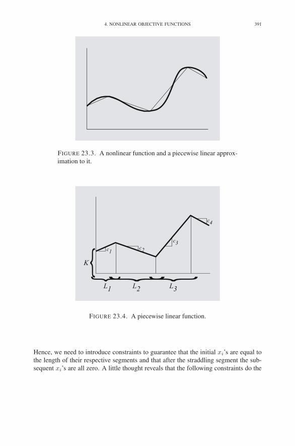
4. NONLINEAR OBJECTIVE FUNCTIONS 391
FIGURE 23.3. A nonlinear function and a piecewise linear approx-
imation to it.
{ {{{
K
L1
L2
L3
c1
c2
c3
c4
FIGURE 23.4. A piecewise linear function.
Hence, we need to introduce constraints to guarantee that the initial xi’s are equal to
the length of their respective segments and that after the straddling segment the sub-
sequent xi’s are all zero. A little thought reveals that the following constraints do the

392 23. INTEGER PROGRAMMING
trick:
Ljwj ≤ xj ≤ Ljwj−1 j = 1, 2, . . . , k
w0 = 1
wj ∈ {0, 1} j = 1, 2, . . . , k
xj ≥ 0 j = 1, 2, . . . , k.
Indeed, it follows from these constraints that wj ≤ wj−1 for j = 1, 2, . . . , k. This
inequality implies that once one of the wj’s is zero, then all the subsequent ones must
be zero. If wj = wj−1 = 1, the two-sided inequality on xj reduces to Lj ≤ xj ≤ Lj .
That is, xj = Lj . Similarly, if wj = wj−1 = 0, then the two-sided inequality reduces
to xj = 0. The only other case is when wj = 0 but wj−1 = 1. In this case, the
two-sided inequality becomes 0 ≤ xj ≤ Lj . Therefore, in all cases, we get what we
want. Now with this decomposition we can write the piecewise linear function as
K + c1x1 + c2x2 + · · · + ckxk.
5. Branch-and-Bound
In the previous sections, we presented a variety of problems that can be formulated
as integer programming problems. As it happens, all of them had the property that the
integer variables took just one of two values, namely, zero or one. However, there
are other integer programming problems in which the integer variables can be any
nonnegative integer. Hence, we define the standard integer programming problem as
follows:
maximize cT x
subject to Ax≤ b
x≥ 0
x has integer components.
In this section, we shall present an algorithm for solving these problems. The algo-
rithm is called branch-and-bound. It involves solving a (potentially) large number of
(related) linear programming problems in its search for an optimal integer solution.
The algorithm starts out with the following wishful approach: first ignore the con-
straint that the components of x be integers, solve the resulting linear programming
problem, and hope that the solution vector has all integer components. Of course,
hopes are almost always unfulfilled, and so a backup strategy is needed. The simplest
strategy would be to round each resulting solution value to its nearest integer value.
Unfortunately, this naive strategy can be quite bad. In fact, the integer solution so ob-
tained might not even be feasible, which shouldn’t be surprising, since we know that
the solution to a linear programming problem is at a vertex of the feasible set and so it
is quite expected that naive movement will go outside of the feasible set.

5. BRANCH-AND-BOUND 393
1 2 3 4 5 60
0
1
2
3
4
5
6
x1
x2
10x1+7x2=40
Optimal Solution
to LP−relaxation
x1+x2=5
17x1+12x2=68.33
=z0
FIGURE 23.5. An integer programming problem. The dots repre-
sent the feasible integer points, and the shaded region shows the
feasible region for the LP-relaxation.
To be concrete, consider the following example:
maximize 17x1 + 12x2
subject to 10x1 + 7x2 ≤ 40
x1 + x2 ≤ 5
x1, x2 ≥ 0
x1, x2 integers.
The linear programming problem obtained by dropping the integrality constraint is
called the LP-relaxation. Since it has fewer constraints, its optimal solution provides
an upper bound ζ0 on the the optimal solution ζ∗ to the integer programming prob-
lem. Figure 23.5 shows the feasible points for the integer programming problem as
well as the feasible polytope for its LP-relaxation. The solution to the LP-relaxation is
at (x1, x2) = (5/3, 10/3), and the optimal objective value is 205/3 = 68.33. Round-
ing each component of this solution to the nearest integer, we get (2, 3), which is not
even feasible. The feasible integer solution that is closest to the LP-optimal solution
is (1, 3), but we can see from Figure 23.5 that this solution is not the optimal solution
to the integer programming problem. In fact, it is easy to see from the figure that

394 23. INTEGER PROGRAMMING
1 2 3 4 5 60
0
1
2
3
4
5
6
x1
x2
P1
P2
FIGURE 23.6. The feasible subregions formed by the first branch.
the optimal integer solution is either (1, 4) or (4, 0). To make the problem interest-
ing, we’ve chosen the objective function to make the more distant point (4, 0) be the
optimal solution.
Of course, we can solve only very small problems by the graphical method: to
solve larger problems, an algorithm is required, which we now describe. Consider
variable x1 in the optimal solution to the LP-relaxation. Its value is 5/3. In the optimal
solution to the integer programming problem, it will be an integer. Hence, it will
satisfy either x1 ≤ 1 or x1 ≥ 2. We consider these two cases separately. Let P1 denote
the linear programming problem obtained by adding the constraint x1 ≤ 1 to the LP-
relaxation, and let P2 denote the problem obtained by including the other possibility,
x1 ≥ 2. The feasible regions for P1 and P2 are shown in Figure 23.6. Let us study
P1 first. It is clear from Figure 23.6 that the optimal solution is at (x1, x2) = (1, 4)with an objective value of 65. Our algorithm has found its first feasible solution to the
integer programming problem. We record this solution as the best-so-far. Of course,
better ones may (in this case, will) come along later.
Now let’s consider P2. Looking at Figure 23.6 and doing a small amount of
calculation, we see that the optimal solution is at (x1, x2) = (2, 20/7). In this case,
the objective function value is 478/7 = 68.29. Now if this value had turned out to be
less than the best-so-far value, then we’d be done, since any integer solution that lies
within the feasible region for P2 would have a smaller value yet. But this is not the

5. BRANCH-AND-BOUND 395
P0: x
1=1.67, x
2=3.33
ζ=68.33
x1<1 x
1>2
x2>3x
2<2
P1: x
1=1, x
2=4
ζ=65
P2: x
1=2, x
2=2.86
ζ=68.29
FIGURE 23.7. The beginnings of the enumeration tree.
case, and so we must continue our systematic search. Since x2 = 20/7 = 2.86, we
divide P2 into two subproblems, one in which the constraint x2 ≤ 2 is added and one
with x2 ≥ 3 added.
Before considering these two new cases, note that we are starting to develop a
tree of linear programming subproblems. This tree is called the enumeration tree. The
tree as far as we have investigated is shown in Figure 23.7. The double box around P1
indicates that that part of the tree is done: i.e., there are no branches emanating from
P1—it is a leaf node. The two empty boxes below P2 indicate two subproblems that
have yet to be studied. Let’s proceed by looking at the left branch, which corresponds
to adding the constraint x2 ≤ 2 to what we had before. We denote this subproblem
by P3. Its feasible region is shown in Figure 23.8, from which we see that the optimal
solution is at (2.6, 2). The associated optimal objective value is 68.2. Again, the
solution is fractional. Hence, the process of subdividing must continue. This time we
subdivide based on the values of x1. Indeed, we consider two cases: either x1 ≤ 2 or
x1 ≥ 3.
Figure 23.9 shows the enumeration tree as it now stands. At this juncture, there
are three directions in which we could proceed. We could either study the other branch
under P2 or work on one of the two branches sitting under P3. If we were to system-
atically solve all the problems on a given level of the tree before going deeper, we
would be performing what is referred to as a breadth-first search. On the other hand,
going deep before going wide is called a depth-first search. For reasons that we shall

396 23. INTEGER PROGRAMMING
1 2 3 4 5 60
0
1
2
3
4
5
6
x1
x2
P1
P3
FIGURE 23.8. The refinement of P2 to P3.
explain later, it turns out to be better to do a depth-first search. And, to be specific, let
us always choose the left branch before the right branch (in practice, there are much
better rules that one can employ here). So our next linear programming problem is the
one that we get by adding the constraint that x1 ≤ 2 to the constraints that defined P3.
Let us call this new problem P4. Its feasible region is shown in Figure 23.10. It is easy
to see that the optimal solution to this problem is (2, 2), with an objective value of 58.
This solution is an integer solution, so it is feasible for the integer programming prob-
lem. But it is not better than our best-so-far. Nonetheless, we do not need to consider
any further subproblems below this one in the enumeration tree.
Since problem P4 is a leaf in the enumeration tree, we need to work back up the
tree looking for the first node that has an unsolved problem sitting under it. For the case
at hand, the unsolved problem is on the right branch underneath P3. Let us call this
problem P5. It too is depicted in Figure 23.10. The optimal solution is (3, 1.43), with
an optimal objective function value of 68.14. Since this objective function value is
larger than the value of the best-so-far integer solution, we must further investigate by
dividing into two possibilities, either x2 ≤ 1 or x2 ≥ 2. At this point, the enumeration
tree looks like that shown in Figure 23.11.
Let P6 denote the linear programming problem that we get on the left branch un-
der P5. Its feasible region is shown in Figure 23.12. The optimal solution is (3.3, 1),and the associated objective value is 68.1. Again, the solution is fractional and has a

5. BRANCH-AND-BOUND 397
P0: x
1=1.67, x
2=3.33
ζ=68.33
P3: x
1=2.6, x
2=2
ζ=68.2
x1<1 x
1>2
x2>3x
2<2
x1<2 x
1>3
P1: x
1=1, x
2=4
ζ=65
P2: x
1=2, x
2=2.86
ζ=68.29
FIGURE 23.9. The enumeration tree after solving P3.
higher objective value than the best-so-far integer solution. Hence, it must be subdi-
vided based on x1 ≤ 3 as opposed to x1 ≥ 4. Denoting these two problems by P7
and P8, their feasible regions are as depicted in Figure 23.13. The solution to P7 is
(3, 1), and the objective value is 63. This is an integer solution, but it is not better than
the best-so-far. Nonetheless, the node becomes a leaf, since the solution is integral.
Hence, we move on to P8. The solution to this problem is also integral, (4, 0). Also,
the objective value associated with this solution is 68, which is a new record for feasi-
ble integer solutions. Hence, this solution becomes our best-so-far. The enumeration
tree at this point is shown in Figure 23.14.
Now we need to go back and solve the problems under P5 and P2 (and any
subproblems thereof). It turns out that both these subproblems are infeasible, and
so no more subdivisions are needed. The enumeration tree is now completely fath-
omed and is shown in Figure 23.15. We can now assert that the optimal solution to
the original integer programming problem was found in problem P8. The solution is
(x1, x2) = (4, 0), and the associated objective function value is 68.

398 23. INTEGER PROGRAMMING
1 2 3 4 5 60
0
1
2
3
4
5
6
x1
x2
P1
P5
P4
FIGURE 23.10. The refinement of P3 to P4.

5. BRANCH-AND-BOUND 399
P0: x
1=1.67, x
2=3.33
ζ=68.33
P3: x
1=2.6, x
2=2
ζ=68.2
x1<1 x
1>2
x2>3x
2<2
x1<2 x
1>3
x2<1 x2
>2
P1: x
1=1, x
2=4
ζ=65
P4: x
1=2, x
2=2
ζ=58
P5: x
1=3, x
2=1.43
ζ=68.14
P2: x
1=2, x
2=2.86
ζ=68.29
FIGURE 23.11. The enumeration tree after solving P5. The double
box around P4 indicates that it is a leaf in the tree.

400 23. INTEGER PROGRAMMING
1 2 3 4 5 60
0
1
2
3
4
5
6
x1
x2
P1
P6
P4
FIGURE 23.12. The refinement of P5 to P6.
1 2 3 4 5 60
0
1
2
3
4
5
6
x1
x2
P1
P7
P5 P
8
FIGURE 23.13. The refinement of P6 to P7 and P8.

5. BRANCH-AND-BOUND 401
P0: x
1=1.67, x
2=3.33
ζ=68.33
P8: x
1=4, x
2=0
ζ=68
P6: x
1=3.3, x
2=1
ζ=68.1
P3: x
1=2.6, x
2=2
ζ=68.2
x1<1 x
1>2
x2>3x
2<2
x1<2 x
1>3
x2<1 x2
>2
x1<3 x
1>4
P1: x
1=1, x
2=4
ζ=65
P4: x
1=2, x
2=2
ζ=58
P7: x
1=3, x
2=1
ζ=63
P5: x
1=3, x
2=1.43
ζ=68.14
P2: x
1=2, x
2=2.86
ζ=68.29
FIGURE 23.14. The enumeration tree after solving P6, P7, and P8.

402 23. INTEGER PROGRAMMING
P0: x
1=1.67, x
2=3.33
ζ=68.33
P8: x
1=4, x
2=0
ζ=68
P6: x
1=3.3, x
2=1
ζ=68.1
P3: x
1=2.6, x
2=2
ζ=68.2
x1<1 x
1>2
x2>3x
2<2
x1<2 x
1>3
x2<1 x2
>2
x1<3 x
1>4
P1: x
1=1, x
2=4
ζ=65
P4: x
1=2, x
2=2
ζ=58
P7: x
1=3, x
2=1
ζ=63
P5: x
1=3, x
2=1.43
ζ=68.14
P2: x
1=2, x
2=2.86
ζ=68.29
P9: Infeasible
P10
: Infeasible
FIGURE 23.15. The complete enumeration tree.
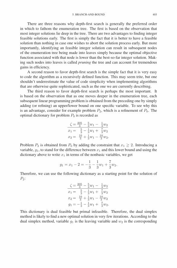
5. BRANCH-AND-BOUND 403
There are three reasons why depth-first search is generally the preferred order
in which to fathom the enumeration tree. The first is based on the observation that
most integer solutions lie deep in the tree. There are two advantages to finding integer
feasible solutions early. The first is simply the fact that it is better to have a feasible
solution than nothing in case one wishes to abort the solution process early. But more
importantly, identifying an feasible integer solution can result in subsequent nodes
of the enumeration tree being made into leaves simply because the optimal objective
function associated with that node is lower than the best-so-far integer solution. Mak-
ing such nodes into leaves is called pruning the tree and can account for tremendous
gains in efficiency.
A second reason to favor depth-first search is the simple fact that it is very easy
to code the algorithm as a recursively defined function. This may seem trite, but one
shouldn’t underestimate the value of code simplicity when implementing algorithms
that are otherwise quite sophisticated, such as the one we are currently describing.
The third reason to favor depth-first search is perhaps the most important. It
is based on the observation that as one moves deeper in the enumeration tree, each
subsequent linear programming problem is obtained from the preceding one by simply
adding (or refining) an upper/lower bound on one specific variable. To see why this
is an advantage, consider for example problem P2, which is a refinement of P0. The
optimal dictionary for problem P0 is recorded as
ζ = 2053 − 5
3w1 − 13w2
x1 = 53 − 1
3w1 + 73w2
x2 = 103 + 1
3w1 − 103 w2.
Problem P2 is obtained from P0 by adding the constraint that x1 ≥ 2. Introducing a
variable, g1, to stand for the difference between x1 and this lower bound and using the
dictionary above to write x1 in terms of the nonbasic variables, we get
g1 = x1 − 2 = −1
3− 1
3w1 +
7
3w2.
Therefore, we can use the following dictionary as a starting point for the solution of
P2:
ζ = 2053 − 5
3w1 − 13w2
x1 = 53 − 1
3w1 + 73w2
x2 = 103 + 1
3w1 − 103 w2
g1 = − 13 − 1
3w1 + 73w2.
This dictionary is dual feasible but primal infeasible. Therefore, the dual simplex
method is likely to find a new optimal solution in very few iterations. According to the
dual simplex method, variable g1 is the leaving variable and w2 is the corresponding
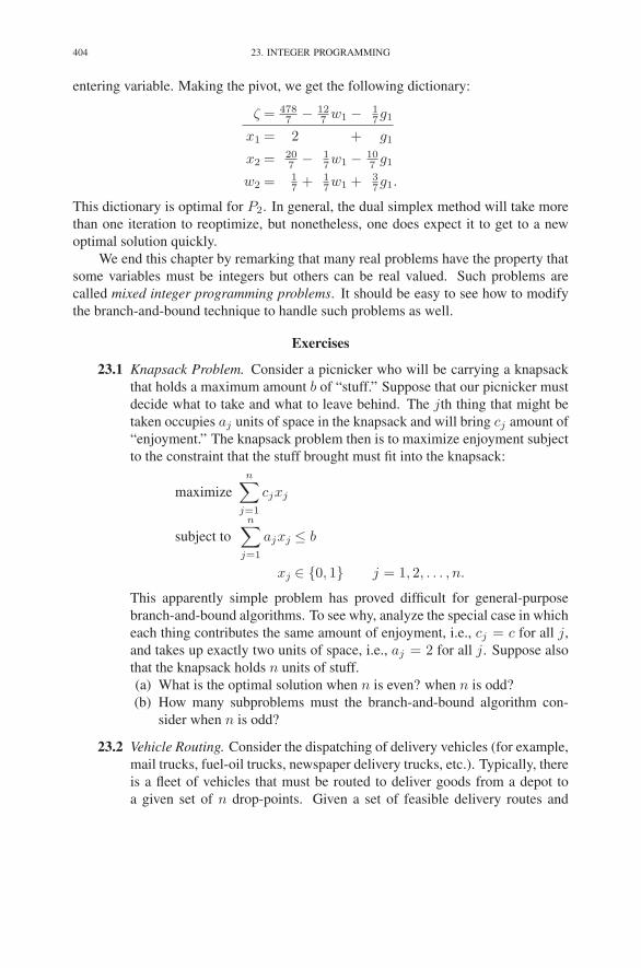
404 23. INTEGER PROGRAMMING
entering variable. Making the pivot, we get the following dictionary:
ζ = 4787 − 12
7 w1 − 17g1
x1 = 2 + g1
x2 = 207 − 1
7w1 − 107 g1
w2 = 17 + 1
7w1 + 37g1.
This dictionary is optimal for P2. In general, the dual simplex method will take more
than one iteration to reoptimize, but nonetheless, one does expect it to get to a new
optimal solution quickly.
We end this chapter by remarking that many real problems have the property that
some variables must be integers but others can be real valued. Such problems are
called mixed integer programming problems. It should be easy to see how to modify
the branch-and-bound technique to handle such problems as well.
Exercises
23.1 Knapsack Problem. Consider a picnicker who will be carrying a knapsack
that holds a maximum amount b of “stuff.” Suppose that our picnicker must
decide what to take and what to leave behind. The jth thing that might be
taken occupies aj units of space in the knapsack and will bring cj amount of
“enjoyment.” The knapsack problem then is to maximize enjoyment subject
to the constraint that the stuff brought must fit into the knapsack:
maximize
n∑
j=1
cjxj
subject to
n∑
j=1
ajxj ≤ b
xj ∈ {0, 1} j = 1, 2, . . . , n.
This apparently simple problem has proved difficult for general-purpose
branch-and-bound algorithms. To see why, analyze the special case in which
each thing contributes the same amount of enjoyment, i.e., cj = c for all j,
and takes up exactly two units of space, i.e., aj = 2 for all j. Suppose also
that the knapsack holds n units of stuff.
(a) What is the optimal solution when n is even? when n is odd?
(b) How many subproblems must the branch-and-bound algorithm con-
sider when n is odd?
23.2 Vehicle Routing. Consider the dispatching of delivery vehicles (for example,
mail trucks, fuel-oil trucks, newspaper delivery trucks, etc.). Typically, there
is a fleet of vehicles that must be routed to deliver goods from a depot to
a given set of n drop-points. Given a set of feasible delivery routes and

NOTES 405
the cost associated with each one, explain how to formulate the problem of
minimizing the total delivery cost as a set-partitioning problem.
23.3 Explain how to modify the integer programming reformulation of continu-
ous piecewise linear functions so that it covers piecewise linear functions
having discontinuities at the junctions of the linear segments. Can fixed
costs be handled with this approach?
Notes
Standard references for integer programming include the classic text by Garfinkel
& Nemhauser (1972) and the more recent text by Nemhauser & Wolsey (1988).

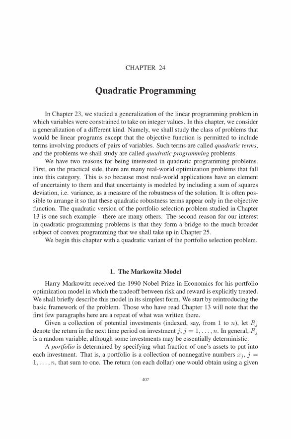
CHAPTER 24
Quadratic Programming
In Chapter 23, we studied a generalization of the linear programming problem in
which variables were constrained to take on integer values. In this chapter, we consider
a generalization of a different kind. Namely, we shall study the class of problems that
would be linear programs except that the objective function is permitted to include
terms involving products of pairs of variables. Such terms are called quadratic terms,
and the problems we shall study are called quadratic programming problems.
We have two reasons for being interested in quadratic programming problems.
First, on the practical side, there are many real-world optimization problems that fall
into this category. This is so because most real-world applications have an element
of uncertainty to them and that uncertainty is modeled by including a sum of squares
deviation, i.e. variance, as a measure of the robustness of the solution. It is often pos-
sible to arrange it so that these quadratic robustness terms appear only in the objective
function. The quadratic version of the portfolio selection problem studied in Chapter
13 is one such example—there are many others. The second reason for our interest
in quadratic programming problems is that they form a bridge to the much broader
subject of convex programming that we shall take up in Chapter 25.
We begin this chapter with a quadratic variant of the portfolio selection problem.
1. The Markowitz Model
Harry Markowitz received the 1990 Nobel Prize in Economics for his portfolio
optimization model in which the tradeoff between risk and reward is explicitly treated.
We shall briefly describe this model in its simplest form. We start by reintroducing the
basic framework of the problem. Those who have read Chapter 13 will note that the
first few paragraphs here are a repeat of what was written there.
Given a collection of potential investments (indexed, say, from 1 to n), let Rj
denote the return in the next time period on investment j, j = 1, . . . , n. In general, Rj
is a random variable, although some investments may be essentially deterministic.
A portfolio is determined by specifying what fraction of one’s assets to put into
each investment. That is, a portfolio is a collection of nonnegative numbers xj , j =1, . . . , n, that sum to one. The return (on each dollar) one would obtain using a given
407

408 24. QUADRATIC PROGRAMMING
portfolio is given by
R =∑
j
xjRj .
The reward associated with such a portfolio is defined as the expected return:
ER =∑
j
xjERj .
If reward alone were the issue, the problem would be trivial: simply put everything in
the investment with the highest expected return. But unfortunately, investments with
high reward typically also carry a high level of risk. That is, even though they are
expected to do very well in the long run, they also tend to be erratic in the short term.
Markowitz defined the risk associated with an investment to be the variance of the
return:
Var(R) = E(R − ER)2
= E
⎛
⎝
∑
j
xj(Rj − ERj)
⎞
⎠
2
= E
⎛
⎝
∑
j
xjRj
⎞
⎠
2
,
where Rj = Rj − ERj . One would like to maximize the reward while at the same
time not incur excessive risk. In the Markowitz model, one forms a linear combination
of the mean and the variance (parametrized here by μ) and minimizes that:
(24.1)
minimize −∑
j
xjERj + μE
⎛
⎝
∑
j
xjRj
⎞
⎠
2
subject to∑
j
xj = 1
xj ≥ 0 j = 1, 2, . . . , n.
Here, as in Chapter 13, μ is a positive parameter that represents the importance of risk
relative to reward: high values of μ tend to minimize risk at the expense of reward,
whereas low values put more weight on reward.
Again, as in Chapter 13, whenever there are individual investments that are neg-
atively correlated, i.e. one is likely to go up exactly on those days where the other is
likely to go down, it is wise to buy some of each. This is called hedging. In statistics,
the so-called covariance matrix is the key to identifying negative correlations. And,
the covariance matrix is what appears in the Markowitz model. To see it, let us expand
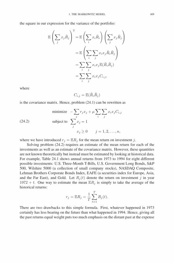
1. THE MARKOWITZ MODEL 409
the square in our expression for the variance of the portfolio:
E
⎛
⎝
∑
j
xjRj
⎞
⎠
2
= E
(
∑
i
xiRi
)
⎛
⎝
∑
j
xjRj
⎞
⎠
= E
⎛
⎝
∑
i
∑
j
xixjRiRj
⎞
⎠
=∑
i
∑
j
xixjE(RiRj)
=∑
i
∑
j
xixjCi,j ,
where
Ci,j = E(RiRj)
is the covariance matrix. Hence, problem (24.1) can be rewritten as
(24.2)
minimize −∑
j
rjxj + μ∑
i
∑
j
xixjCi,j
subject to∑
j
xj = 1
xj ≥ 0 j = 1, 2, . . . , n,
where we have introduced rj = ERj for the mean return on investment j.
Solving problem (24.2) requires an estimate of the mean return for each of the
investments as well as an estimate of the covariance matrix. However, these quantities
are not known theoretically but instead must be estimated by looking at historical data.
For example, Table 24.1 shows annual returns from 1973 to 1994 for eight different
possible investments: U.S. Three-Month T-Bills, U.S. Government Long Bonds, S&P
500, Wilshire 5000 (a collection of small company stocks), NASDAQ Composite,
Lehman Brothers Corporate Bonds Index, EAFE (a securities index for Europe, Asia,
and the Far East), and Gold. Let Rj(t) denote the return on investment j in year
1972 + t. One way to estimate the mean ERj is simply to take the average of the
historical returns:
rj = ERj =1
T
T∑
t=1
Rj(t).
There are two drawbacks to this simple formula. First, whatever happened in 1973
certainly has less bearing on the future than what happened in 1994. Hence, giving all
the past returns equal weight puts too much emphasis on the distant past at the expense
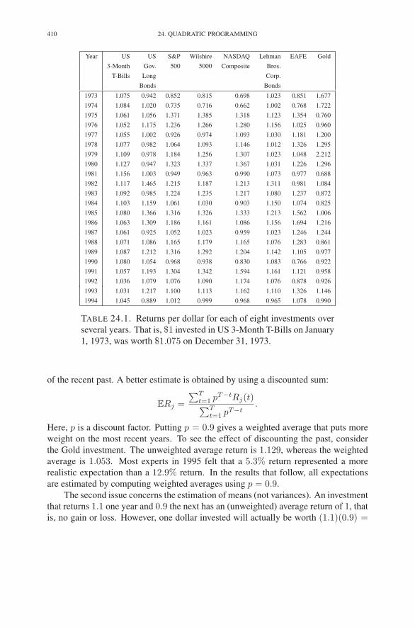
410 24. QUADRATIC PROGRAMMING
Year US US S&P Wilshire NASDAQ Lehman EAFE Gold
3-Month Gov. 500 5000 Composite Bros.
T-Bills Long Corp.
Bonds Bonds
1973 1.075 0.942 0.852 0.815 0.698 1.023 0.851 1.677
1974 1.084 1.020 0.735 0.716 0.662 1.002 0.768 1.722
1975 1.061 1.056 1.371 1.385 1.318 1.123 1.354 0.760
1976 1.052 1.175 1.236 1.266 1.280 1.156 1.025 0.960
1977 1.055 1.002 0.926 0.974 1.093 1.030 1.181 1.200
1978 1.077 0.982 1.064 1.093 1.146 1.012 1.326 1.295
1979 1.109 0.978 1.184 1.256 1.307 1.023 1.048 2.212
1980 1.127 0.947 1.323 1.337 1.367 1.031 1.226 1.296
1981 1.156 1.003 0.949 0.963 0.990 1.073 0.977 0.688
1982 1.117 1.465 1.215 1.187 1.213 1.311 0.981 1.084
1983 1.092 0.985 1.224 1.235 1.217 1.080 1.237 0.872
1984 1.103 1.159 1.061 1.030 0.903 1.150 1.074 0.825
1985 1.080 1.366 1.316 1.326 1.333 1.213 1.562 1.006
1986 1.063 1.309 1.186 1.161 1.086 1.156 1.694 1.216
1987 1.061 0.925 1.052 1.023 0.959 1.023 1.246 1.244
1988 1.071 1.086 1.165 1.179 1.165 1.076 1.283 0.861
1989 1.087 1.212 1.316 1.292 1.204 1.142 1.105 0.977
1990 1.080 1.054 0.968 0.938 0.830 1.083 0.766 0.922
1991 1.057 1.193 1.304 1.342 1.594 1.161 1.121 0.958
1992 1.036 1.079 1.076 1.090 1.174 1.076 0.878 0.926
1993 1.031 1.217 1.100 1.113 1.162 1.110 1.326 1.146
1994 1.045 0.889 1.012 0.999 0.968 0.965 1.078 0.990
TABLE 24.1. Returns per dollar for each of eight investments over
several years. That is, $1 invested in US 3-Month T-Bills on January
1, 1973, was worth $1.075 on December 31, 1973.
of the recent past. A better estimate is obtained by using a discounted sum:
ERj =
∑Tt=1 pT−tRj(t)∑T
t=1 pT−t.
Here, p is a discount factor. Putting p = 0.9 gives a weighted average that puts more
weight on the most recent years. To see the effect of discounting the past, consider
the Gold investment. The unweighted average return is 1.129, whereas the weighted
average is 1.053. Most experts in 1995 felt that a 5.3% return represented a more
realistic expectation than a 12.9% return. In the results that follow, all expectations
are estimated by computing weighted averages using p = 0.9.
The second issue concerns the estimation of means (not variances). An investment
that returns 1.1 one year and 0.9 the next has an (unweighted) average return of 1, that
is, no gain or loss. However, one dollar invested will actually be worth (1.1)(0.9) =
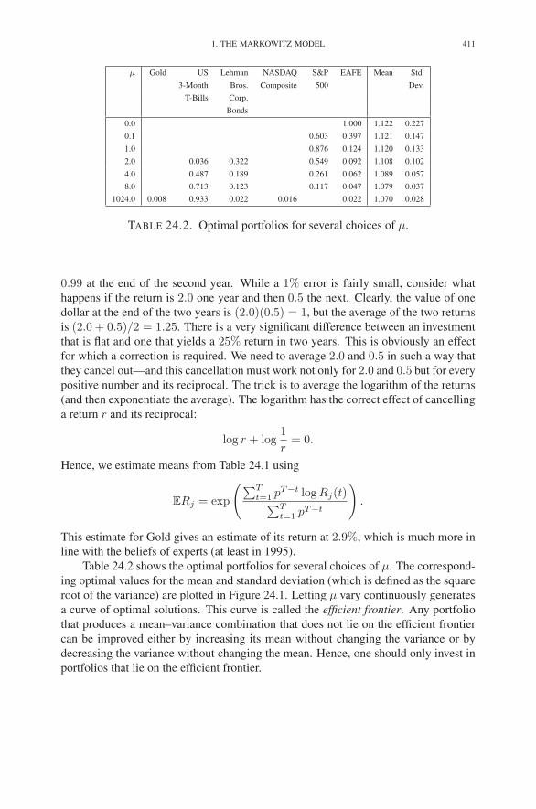
1. THE MARKOWITZ MODEL 411
μ Gold US Lehman NASDAQ S&P EAFE Mean Std.
3-Month Bros. Composite 500 Dev.
T-Bills Corp.
Bonds
0.0 1.000 1.122 0.227
0.1 0.603 0.397 1.121 0.147
1.0 0.876 0.124 1.120 0.133
2.0 0.036 0.322 0.549 0.092 1.108 0.102
4.0 0.487 0.189 0.261 0.062 1.089 0.057
8.0 0.713 0.123 0.117 0.047 1.079 0.037
1024.0 0.008 0.933 0.022 0.016 0.022 1.070 0.028
TABLE 24.2. Optimal portfolios for several choices of μ.
0.99 at the end of the second year. While a 1% error is fairly small, consider what
happens if the return is 2.0 one year and then 0.5 the next. Clearly, the value of one
dollar at the end of the two years is (2.0)(0.5) = 1, but the average of the two returns
is (2.0 + 0.5)/2 = 1.25. There is a very significant difference between an investment
that is flat and one that yields a 25% return in two years. This is obviously an effect
for which a correction is required. We need to average 2.0 and 0.5 in such a way that
they cancel out—and this cancellation must work not only for 2.0 and 0.5 but for every
positive number and its reciprocal. The trick is to average the logarithm of the returns
(and then exponentiate the average). The logarithm has the correct effect of cancelling
a return r and its reciprocal:
log r + log1
r= 0.
Hence, we estimate means from Table 24.1 using
ERj = exp
(
∑Tt=1 pT−t log Rj(t)
∑Tt=1 pT−t
)
.
This estimate for Gold gives an estimate of its return at 2.9%, which is much more in
line with the beliefs of experts (at least in 1995).
Table 24.2 shows the optimal portfolios for several choices of μ. The correspond-
ing optimal values for the mean and standard deviation (which is defined as the square
root of the variance) are plotted in Figure 24.1. Letting μ vary continuously generates
a curve of optimal solutions. This curve is called the efficient frontier. Any portfolio
that produces a mean–variance combination that does not lie on the efficient frontier
can be improved either by increasing its mean without changing the variance or by
decreasing the variance without changing the mean. Hence, one should only invest in
portfolios that lie on the efficient frontier.
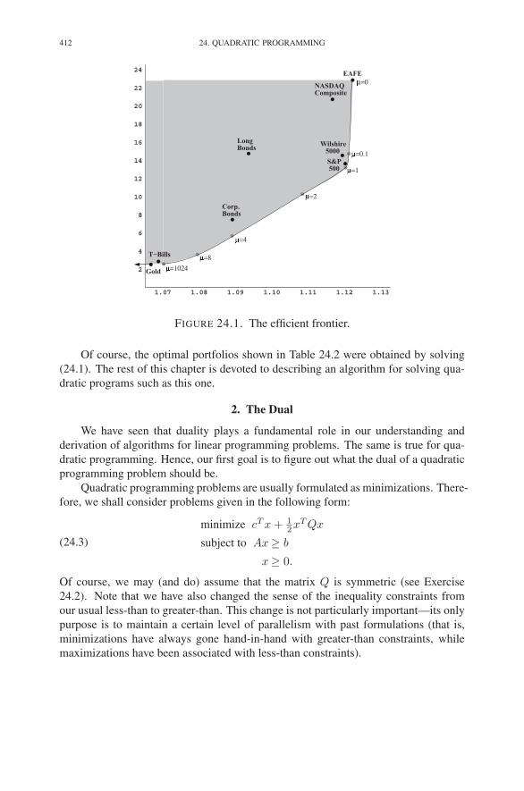
412 24. QUADRATIC PROGRAMMING
Wilshire 5000 µ=0.1
µ=1
1.08 1.09 1.10 1.11 1.12 1.131.07
2
6
8
10
12
14
16
18
20
22
24
4 T−Bills
Corp.Bonds
LongBonds
S&P 500
NASDAQComposite
Gold
EAFE
µ=8
µ=4
µ=2
µ=0
µ=1024
FIGURE 24.1. The efficient frontier.
Of course, the optimal portfolios shown in Table 24.2 were obtained by solving
(24.1). The rest of this chapter is devoted to describing an algorithm for solving qua-
dratic programs such as this one.
2. The Dual
We have seen that duality plays a fundamental role in our understanding and
derivation of algorithms for linear programming problems. The same is true for qua-
dratic programming. Hence, our first goal is to figure out what the dual of a quadratic
programming problem should be.
Quadratic programming problems are usually formulated as minimizations. There-
fore, we shall consider problems given in the following form:
(24.3)
minimize cT x + 12xT Qx
subject to Ax≥ b
x≥ 0.
Of course, we may (and do) assume that the matrix Q is symmetric (see Exercise
24.2). Note that we have also changed the sense of the inequality constraints from
our usual less-than to greater-than. This change is not particularly important—its only
purpose is to maintain a certain level of parallelism with past formulations (that is,
minimizations have always gone hand-in-hand with greater-than constraints, while
maximizations have been associated with less-than constraints).
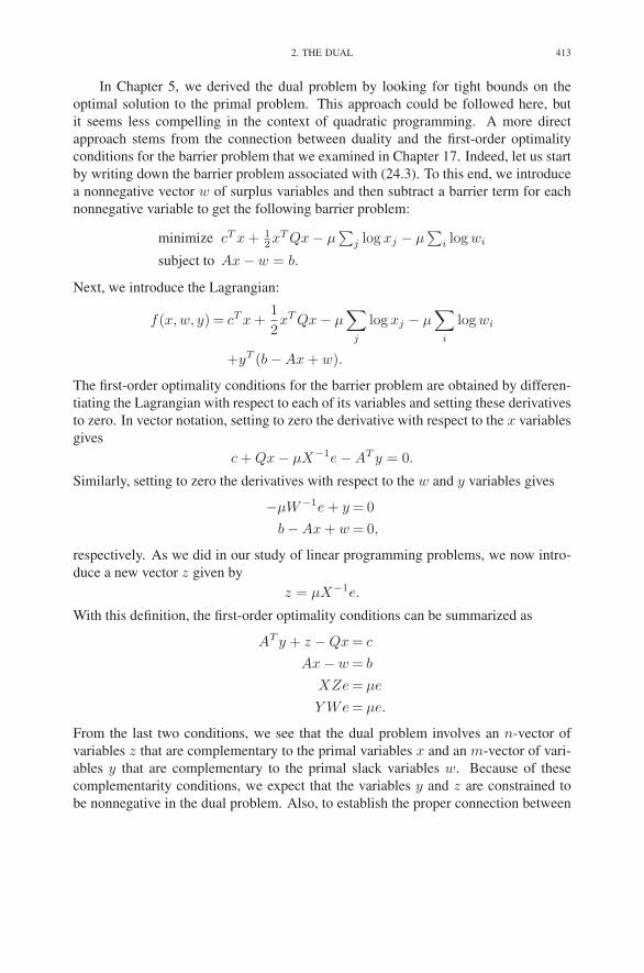
2. THE DUAL 413
In Chapter 5, we derived the dual problem by looking for tight bounds on the
optimal solution to the primal problem. This approach could be followed here, but
it seems less compelling in the context of quadratic programming. A more direct
approach stems from the connection between duality and the first-order optimality
conditions for the barrier problem that we examined in Chapter 17. Indeed, let us start
by writing down the barrier problem associated with (24.3). To this end, we introduce
a nonnegative vector w of surplus variables and then subtract a barrier term for each
nonnegative variable to get the following barrier problem:
minimize cT x + 12xT Qx − μ
∑
j log xj − μ∑
i log wi
subject to Ax − w = b.
Next, we introduce the Lagrangian:
f(x,w, y) = cT x +1
2xT Qx − μ
∑
j
log xj − μ∑
i
log wi
+yT (b − Ax + w).
The first-order optimality conditions for the barrier problem are obtained by differen-
tiating the Lagrangian with respect to each of its variables and setting these derivatives
to zero. In vector notation, setting to zero the derivative with respect to the x variables
gives
c + Qx − μX−1e − AT y = 0.
Similarly, setting to zero the derivatives with respect to the w and y variables gives
−μW−1e + y = 0
b − Ax + w = 0,
respectively. As we did in our study of linear programming problems, we now intro-
duce a new vector z given by
z = μX−1e.
With this definition, the first-order optimality conditions can be summarized as
AT y + z − Qx = c
Ax − w = b
XZe = μe
Y We = μe.
From the last two conditions, we see that the dual problem involves an n-vector of
variables z that are complementary to the primal variables x and an m-vector of vari-
ables y that are complementary to the primal slack variables w. Because of these
complementarity conditions, we expect that the variables y and z are constrained to
be nonnegative in the dual problem. Also, to establish the proper connection between
414 24. QUADRATIC PROGRAMMING
the first-order optimality conditions and the dual problem, we must recognize the first
condition as a dual constraint. Hence, the constraints for the dual problem are
AT y + z − Qx = c
y, z ≥ 0.
It is interesting to note that the dual constraints involve an n-vector x that seems as
if it should belong to the primal problem. This may seem odd, but when understood
properly it turns out to be entirely harmless. The correct interpretation is that the
variable x appearing in the dual has, in principle, no connection to the variable xappearing in the primal (except that, as we shall soon see, at optimality they will be
equal).
The barrier problem has helped us write down the dual constraints, but it does not
shed any light on the dual objective function. To see what the dual objective function
should be, we look at what it needs to be for the weak duality theorem to hold true. In
the weak duality theorem, we assume that we have a primal feasible solution (x,w)and a dual feasible solution (x, y, z). We then follow the obvious chains of equalities:
yT (Ax) = yT (b + w) = bT y + yT w
and
(AT y)T x = (c − z + Qx)T x = cT x − zT x + xT Qx.
Now, since yT (Ax) = (AT y)T x, we see that
0 ≤ yT w + zT x = cT x + xT Qx − bT y
= (cT x +1
2xT Qx) − (bT y − 1
2xT Qx).
From this inequality, we see that the dual objective function is bT y − 12xT Qx. Hence,
the dual problem can be stated now as
maximize bT y − 12xT Qx
subject to AT y + z − Qx = c
y, z ≥ 0.
For linear programming, the fundamental connection between the primal and dual
problems is summarized in the Complementary Slackness Theorem. In the next sec-
tion, we shall derive a version of this theorem for quadratic programming.
3. Convexity and Complexity
In linear programming, the dual problem is important because it provides a cer-
tificate of optimality as manifest in the Complementary Slackness Theorem. Under
certain conditions, the same is true here. Let us start by deriving the analogue of the
Complementary Slackness Theorem. The derivation begins with a reiteration of the
derivation of the Weak Duality Theorem. Indeed, let (x,w) denote a feasible solution

3. CONVEXITY AND COMPLEXITY 415
to the primal problem and let (x, y, z) denote a feasible solution to the dual problem
(we have put a bar on the dual x to distinguish it from the one appearing in the pri-
mal). The chain of equalities that form the backbone of the proof of the Weak Duality
Theorem are, as always, obtained by writing yT Ax two ways, namely,
yT (Ax) = (AT y)T x,
and then producing the obvious substitutions
yT (Ax) = yT (b + w) = bT y + yT w
and
(AT y)T x = (c − z + Qx)T x = cT x − zT x + xT Qx.
Comparing the ends of these two chains and using the fact that both yT w and zT x are
nonnegative, we see that
(24.4) 0 ≤ yT w + zT x = cT x + xT Qx − bT y.
So far, so good.
Now, what about the Complementary Slackness Theorem? In the present context,
we expect this theorem to say roughly the following: given a solution (x∗, w∗) that is
feasible for the primal and a solution (x∗, y∗, z∗) that is feasible for the dual, if these
solutions make inequality (24.4) into an equality, then the primal solution is optimal
for the primal problem and the dual solution is optimal for the dual problem.
Let’s try to prove this. Let (x,w) be an arbitrary primal feasible solution. Weak
duality applied to (x,w) on the primal side and (x∗, y∗, z∗) on the dual side says that
cT x + x∗T Qx − bT y∗ ≥ 0.
But for the specific primal feasible solution (x∗, w∗), this inequality is an equality:
cT x∗ + x∗T Qx∗ − bT y∗ = 0.
Combining these, we get
cT x∗ + x∗T Qx∗ ≤ cT x + x∗T Qx.
This is close to what we want, but not quite it. Recall that our aim is to show that the
primal objective function evaluated at x∗ is no larger than its value at x. That is,
cT x∗ +1
2x∗T Qx∗ ≤ cT x +
1
2xT Qx.

416 24. QUADRATIC PROGRAMMING
It is easy to get from the one to the other. Starting from the desired left-hand side, we
compute as follows:
cT x∗ +1
2x∗T Qx∗ = cT x∗ + x∗T Qx∗ − 1
2x∗T Qx∗
≤ cT x + x∗T Qx − 1
2x∗T Qx∗
= cT x +1
2xT Qx − 1
2xT Qx + x∗T Qx − 1
2x∗T Qx∗
= cT x +1
2xT Qx − 1
2(x − x∗)T Q(x − x∗).
The last step in the derivation is to drop the subtracted term on the right-hand side of
the last expression. We can do this if the quantity being subtracted is nonnegative.
But is it? In general, the answer is no. For example, if Q were the negative of the
identity matrix, then the expression (x − x∗)T Q(x − x∗) would be negative rather
than nonnegative.
So it is here that we must impose a restriction on the class of quadratic program-
ming problems that we study. The correct assumption is that Q is positive semidefinite.
Recall from Chapter 19 that a matrix Q is positive semidefinite if
ξT Qξ ≥ 0 for all ξ ∈ Rn.
With this assumption, we can finish the chain of inequalities and conclude that
cT x∗ +1
2x∗T Qx∗ ≤ cT x +
1
2xT Qx.
Since x was an arbitrary primal feasible point, it follows that x∗ (together with w∗)
is optimal for the primal problem. A similar analysis shows that y∗ (together with x∗
and z∗) is optimal for the dual problem (see Exercise 24.4).
A quadratic programming problem of the form (24.3) in which the matrix Q is
positive semidefinite is called a convex quadratic programming problem. The discus-
sion given above can be summarized in the following theorem:
THEOREM 24.1. For convex quadratic programming problems, given a solution
(x∗, w∗) that is feasible for the primal and a solution (x∗, y∗, z∗) that is feasible for
the dual, if these solutions make inequality (24.4) into an equality, then the primal
solution is optimal for the primal problem and the dual solution is optimal for the
dual problem.
To see how bad things are when Q is not positive semidefinite, consider the fol-
lowing example:
(24.5)minimize
∑
j xj(1 − xj) +∑
j cjxj
subject to 0 ≤ xj ≤ 1, j = 1, 2, . . . , n.
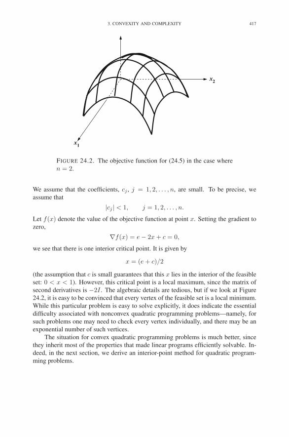
3. CONVEXITY AND COMPLEXITY 417
x1
x2
FIGURE 24.2. The objective function for (24.5) in the case where
n = 2.
We assume that the coefficients, cj , j = 1, 2, . . . , n, are small. To be precise, we
assume that
|cj | < 1, j = 1, 2, . . . , n.
Let f(x) denote the value of the objective function at point x. Setting the gradient to
zero,
∇f(x) = e − 2x + c = 0,
we see that there is one interior critical point. It is given by
x = (e + c)/2
(the assumption that c is small guarantees that this x lies in the interior of the feasible
set: 0 < x < 1). However, this critical point is a local maximum, since the matrix of
second derivatives is −2I . The algebraic details are tedious, but if we look at Figure
24.2, it is easy to be convinced that every vertex of the feasible set is a local minimum.
While this particular problem is easy to solve explicitly, it does indicate the essential
difficulty associated with nonconvex quadratic programming problems—namely, for
such problems one may need to check every vertex individually, and there may be an
exponential number of such vertices.
The situation for convex quadratic programming problems is much better, since
they inherit most of the properties that made linear programs efficiently solvable. In-
deed, in the next section, we derive an interior-point method for quadratic program-
ming problems.
418 24. QUADRATIC PROGRAMMING
4. Solution Via Interior-Point Methods
In this section, we derive an interior-point method for quadratic programming
problems. We start from the first-order optimality conditions, which we saw in the last
section are given by
AT y + z − Qx = c
Ax − w = b
XZe = μe
Y We = μe.
Following the derivation given in Chapter 18, we replace (x,w, y, z) with (x+∆x,w+∆w, y + ∆y, z + ∆z) to get the following nonlinear system in (∆x,∆w,∆y,∆z):
AT ∆y + ∆z − Q∆x = c − AT y − z + Qx =: σ
A∆x − ∆w = b − Ax + w =: ρ
Z∆x + X∆z + ∆X∆Ze = μe − XZe
W∆y + Y ∆w + ∆Y ∆We = μe − Y We.
Next, we drop the nonlinear terms to get the following linear system for the step di-
rections (∆x,∆w,∆y,∆z):
AT ∆y + ∆z − Q∆x = σ
A∆x − ∆w = ρ
Z∆x + X∆z = μe − XZe
W∆y + Y ∆w = μe − Y We.
Following the reductions of Chapter 19, we use the last two equations to solve for ∆zand ∆w to get
∆z = X−1(μe − XZe − Z∆x)
∆w = Y −1(μe − Y We − W∆y).
We then use these expressions to eliminate ∆z and ∆w from the remaining two equa-
tions in the system. After elimination, we arrive at the following reduced KKT system:
AT ∆y − (X−1Z + Q)∆x = σ − μX−1e + z(24.6)
A∆x + Y −1W∆y = ρ + μY −1e − w.(24.7)
Substituting in the definitions of ρ and σ and writing the system in matrix notation,
we get[
−(X−1Z + Q) AT
A Y −1W
][
∆x
∆y
]
=
[
c − AT y − μX−1e + Qx
b − Ax + μY −1e
]
.
A summary of the algorithm is shown in Figure 24.3. It should be clear that

5. PRACTICAL CONSIDERATIONS 419
initialize (x,w, y, z) > 0
while (not optimal) {ρ = b − Ax + w
σ = c − AT y − z + Qx
γ = zT x + yT w
μ = δγ
n + msolve:
[
−(X−1Z + Q) AT
A Y −1W
][
∆x
∆y
]
=
[
c − AT y − μX−1e + Qx
b − Ax + μY −1e
]
.
∆z = X−1(μe − XZe − Z∆x)
∆w = Y −1(μe − Y We − W∆y)
θ = r
(
maxij
{
−∆xj
xj,−∆wi
wi,−∆yi
yi,−∆zj
zj
})−1
∧ 1
x ← x + θ∆x, w ← w + θ∆w
y ← y + θ∆y, z ← z + θ∆z
}
FIGURE 24.3. The path-following method for quadratic program-
ming problems.
the quadratic term in the objective function plays a fairly small role. In fact, the
convergence analysis given in Chapter 18 can be easily adapted to yield analogous
results for quadratic programming problems (see Exercise 24.6).
5. Practical Considerations
For practical implementations of interior-point algorithms, we saw in Chapter 19
that the difficulties created by dense rows/columns suggest that we solve the reduced
KKT system using an equation solver that can handle symmetric indefinite systems
(such as those described in Chapter 20). Quadratic programming problems give us
420 24. QUADRATIC PROGRAMMING
even more reason to prefer the reduced KKT system. To see why, let us reduce the
system further to get a feel for the normal equations for quadratic programming.
If we use (24.6) to solve for ∆x and then eliminate it from (24.7), we get
∆x = −(X−1Z + Q)−1(
c − AT y + Qx − μX−1e − AT ∆y)
and the associated system of normal equations (in primal form):
(
A(X−1Z + Q)−1AT + Y −1W)
∆y = b − Ax + μY −1e
+A(X−1Z + Q)−1(
c − AT y + Qx − μX−1e)
.
As we saw in Chapter 19, the most significant disadvantage of the normal equations
is that they could involve a dense matrix even when the original constraint matrix is
sparse. For quadratic programming, this disadvantage is even more pronounced. Now
the matrix of normal equations has the nonzero pattern of A(D + Q)−1AT , where Dis a diagonal matrix. If Q is a diagonal matrix, then this matrix appearing between
A and AT is diagonal, and the system has the same structure as we saw for linear
programming. But if Q is not a diagonal matrix, then all hope for any sparsity in
A(D + Q)−1AT is lost.
Fortunately, however, the dual form of the normal equations is likely to retain
some sparsity. Indeed, to derive the dual form, we use (24.7) to solve for ∆y and then
eliminate it from (24.6). The result is
∆y = Y W−1(
b − Ax + μY −1e − A∆x)
and
−(
X−1Z + Q + AT Y W−1A)
∆x = c − AT y + Qx − μX−1e
−AT Y W−1(
b − Ax + μY −1e)
.
Now the matrix has a nonzero pattern of AT A + Q. This pattern is much more likely
to be sparse than the pattern we had above.
As mentioned earlier, there is significantly less risk of fill-in if Q is diagonal. A
quadratic programming problem for which Q is diagonal is called a separable qua-
dratic programming problem. It turns out that every nonseparable quadratic program-
ming problem can be replaced by an equivalent separable version, and sometimes this
replacement results in a problem that can be solved dramatically faster than the origi-
nal nonseparable problem. The trick reveals itself when we remind ourselves that the
problems we are studying are convex quadratic programs, and so we ask the question:
how do we know that the matrix Q is positive semidefinite? Or, more to the point, how
does the creator of the model know that Q is positive semidefinite? There are many
equivalent characterizations of positive semidefiniteness, but the one that is easiest to
check is the one that says that Q is positive semidefinite if and only if it can be factored
as follows:
Q = FT DF.
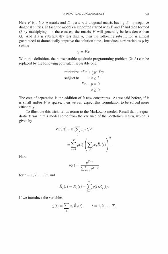
5. PRACTICAL CONSIDERATIONS 421
Here F is a k × n matrix and D is a k × k diagonal matrix having all nonnegative
diagonal entries. In fact, the model creator often started with F and D and then formed
Q by multiplying. In these cases, the matrix F will generally be less dense than
Q. And if k is substantially less than n, then the following substitution is almost
guaranteed to dramatically improve the solution time. Introduce new variables y by
setting
y = Fx.
With this definition, the nonseparable quadratic programming problem (24.3) can be
replaced by the following equivalent separable one:
minimize cT x + 12yT Dy
subject to Ax≥ b
Fx − y = 0
x≥ 0.
The cost of separation is the addition of k new constraints. As we said before, if kis small and/or F is sparse, then we can expect this formulation to be solved more
efficiently.
To illustrate this trick, let us return to the Markowitz model. Recall that the qua-
dratic terms in this model come from the variance of the portfolio’s return, which is
given by
Var(R) = E(∑
j
xjRj)2
=T∑
t=1
p(t)
⎛
⎝
∑
j
xjRj(t)
⎞
⎠
2
.
Here,
p(t) =pT−t
∑Ts=1 pT−s
for t = 1, 2, . . . , T , and
Rj(t) = Rj(t) −T∑
t=1
p(t)Rj(t).
If we introduce the variables,
y(t) =∑
j
xjRj(t), t = 1, 2, . . . , T,

422 24. QUADRATIC PROGRAMMING
then we get the following separable version of the Markowitz model:
maximize∑
j
xjERj − μ
T∑
t=1
p(t)y(t)2
subject to∑
j
xj = 1
y(t) =∑
j xjRj(t), t = 1, 2, . . . , T,
xj ≥ 0 j = 1, 2, . . . , n.
Using specific data involving 500 possible investments and 20 historical time periods,
the separable version solves 60 times faster than the nonseparable version using a
QP-solver called LOQO.
Exercises
24.1 Show that the gradient of the function
f(x) =1
2xT Qx
is given by
∇f(x) = Qx.
24.2 Suppose that Q is an n × n matrix that is not necessarily symmetric. Let
Q = 12 (Q + QT ). Show that
(a) xT Qx = xT Qx, for every x ∈ Rn, and
(b) Q is symmetric.
24.3 Penalty Methods.
(a) Consider the following problem:
minimize 12xT Qx
subject to Ax = b,
where Q is symmetric, positive semidefinite, and invertible (these last
two conditions are equivalent to saying that Q is positive definite). By
solving the first-order optimality conditions, give an explicit formula
for the solution to this problem.
(b) Each equality constraint in the above problem can be replaced by a
penalty term added to the objective function. Penalty terms should be
small when the associated constraint is satisfied and become rapidly
larger as it becomes more and more violated. One choice of penalty
function is the quadratic function. The quadratic penalty problem is
defined as follows:
minimize1
2xT Qx +
λ
2(b − Ax)T (b − Ax),

NOTES 423
where λ is a large real-valued parameter. Derive an explicit formula for
the solution to this problem.
(c) Show that, in the limit as λ tends to infinity, the solution to the quadratic
penalty problem converges to the solution to the original problem.
24.4 Consider a convex quadratic programming problem. Suppose that (x∗, w∗)is a feasible solution for the primal and that (x∗, y∗, z∗) is a feasible solution
for the dual. Suppose further that these solutions make inequality (24.4) into
an equality. Show that the dual solution is optimal for the dual problem.
24.5 A real-valued function f defined on Rn is called convex if, for every x, y ∈
Rn, and for every 0 < t < 1,
f(tx + (1 − t)y) ≤ tf(x) + (1 − t)f(y).
Show that the function
f(x) = cT x +1
2xT Qx, x ∈ R
n,
is convex if Q is positive semidefinite.
24.6 Extend the convergence analysis given in Chapter 18 so that it applies to con-
vex quadratic programming problems, and identify in particular any steps
that depend on Q being positive semidefinite.
24.7 Consider the quadratic programming problem given in the following form:
minimize cT x + 12xT Qx
subject to Ax ≥ b,
(i.e., without assuming nonnegativity of the x vector). Show that the formu-
las for the step directions ∆x and ∆y are given by the following reduced
KKT system:
(24.8)
[
−Q AT
A WY −1
][
∆x
∆y
]
=
[
c − AT y + Qx
b − Ax + μY −1e
]
.
Notes
The portfolio optimization model presented in Section 24.1 was first introduced
by Markowitz (1959). He received the 1990 Nobel Prize in Economics for this work.
Quadratic programming is the simplest class of problems from the subject called
nonlinear programming. Two excellent recent texts that cover nonlinear programming
are those by Bertsekas (1995) and Nash & Sofer (1996). The first paper that extended
the path-following method to quadratic programming was Monteiro & Adler (1989).
The presentation given here follows Vanderbei (1999).


CHAPTER 25
Convex Programming
In the last chapter, we saw that small modifications to the primal–dual interior-
point algorithm allow it to be applied to quadratic programming problems as long as
the quadratic objective function is convex. In this chapter, we shall go further and
allow the objective function to be a general (smooth) convex function. In addition,
we shall allow the feasible region to be any convex set given by a finite collection of
convex inequalities.
1. Differentiable Functions and Taylor Approximations
In this chapter, all nonlinear functions will be assumed to be twice differentiable,
and the second derivatives will be assumed continuous. We begin by reiterating a few
definitions and results that were briefly touched on in Chapter 17. First of all, given a
real-valued function f defined on a domain in Rn, the vector
∇f(x) =
⎡
⎢
⎢
⎢
⎢
⎢
⎣
∂f∂x1
(x)∂f∂x2
(x)...
∂f∂xn
(x)
⎤
⎥
⎥
⎥
⎥
⎥
⎦
is called the gradient of f at x. The matrix
Hf(x) =
⎡
⎢
⎢
⎢
⎢
⎢
⎣
∂2f∂x2
1
(x) ∂2f∂x1∂x2
(x) · · · ∂2f∂x1∂xn
(x)∂2f
∂x2∂x1(x) ∂2f
∂x22
(x) · · · ∂2f∂x2∂xn
(x)
......
...∂2f
∂xn∂x1(x) ∂2f
∂xn∂x2(x) · · · ∂2f
∂x2n(x)
⎤
⎥
⎥
⎥
⎥
⎥
⎦
is called the Hessian of f at x. In dimensions greater than one, the gradient and
the Hessian are the analogues of the first and second derivatives of a function in one
dimension. In particular, they appear in the three-term Taylor series expansion of fabout the point x:
f(x + ∆x) = f(x) + ∇f(x)T ∆x +1
2∆xT Hf(x)∆x + rx(∆x).
425

426 25. CONVEX PROGRAMMING
The last term is called the remainder term. The value of this expansion lies in the fact
that this remainder is small when ∆x is small. To be precise, the remainder has the
following property:
lim∆x→0
rx(∆x)
‖∆x‖2= 0.
This result follows immediately from the one-dimensional three-term Taylor series
expansion applied to g(t) = f(x + t∆x) and the chain rule (see Exercise 25.8).
2. Convex and Concave Functions
There are several equivalent definitions of convexity of a function. The definition
that is most expedient for our purposes is the multidimensional generalization of the
statement that a function is convex if its second derivative is nonnegative. Hence, we
say that a real-valued function defined on a domain in Rn is convex if its Hessian is
positive semidefinite everywhere in its domain. A function is called concave if its
negation is convex.
3. Problem Formulation
We shall study convex optimization problems posed in the following form:
minimize c(x)
subject to ai(x) ≥ bi, i = 1, 2, . . . , m.
Here, the real-valued function c(·) is assumed to be convex, and the m real-valued
functions ai(·) are assumed to be concave. This formulation is the natural extension
of the convex quadratic programming problem studied in the previous chapter, except
that we have omitted the nonnegativity constraints on the variables. This omission is
only a matter of convenience since, if a given problem involves nonnegative variables,
the assertion of their nonnegativity can be incorporated as part of the m nonlinear
inequality constraints. Also note that once we allow for general concave inequality
constraints, we can take the right-hand sides to be zero by simply incorporating ap-
propriate shifts into the nonlinear constraint functions. Hence, many texts on convex
optimization prefer to formulate the constraints in the form ai(x) ≥ 0. We have
left the constants bi on the right-hand side for later comparisons with the quadratic
programming problem of the previous chapter. Finally, note that many convex and
concave functions become infinite in places and therefore have a natural domain that
is a strict subset of Rn. This issue is important to address when solving practical prob-
lems, but since this chapter is just an introduction to convex optimization, we shall
assume that all functions are finite on all of Rn.
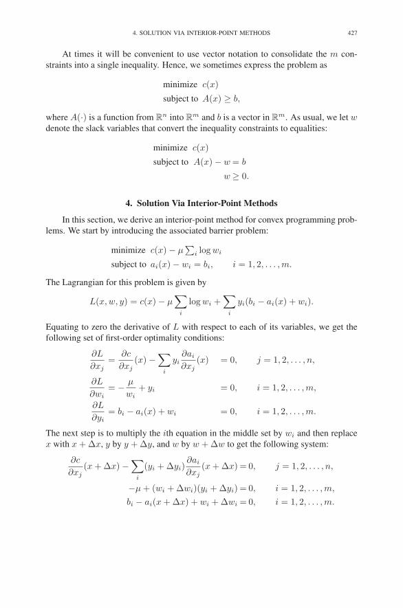
4. SOLUTION VIA INTERIOR-POINT METHODS 427
At times it will be convenient to use vector notation to consolidate the m con-
straints into a single inequality. Hence, we sometimes express the problem as
minimize c(x)
subject to A(x) ≥ b,
where A(·) is a function from Rn into R
m and b is a vector in Rm. As usual, we let w
denote the slack variables that convert the inequality constraints to equalities:
minimize c(x)
subject to A(x) − w = b
w ≥ 0.
4. Solution Via Interior-Point Methods
In this section, we derive an interior-point method for convex programming prob-
lems. We start by introducing the associated barrier problem:
minimize c(x) − μ∑
i log wi
subject to ai(x) − wi = bi, i = 1, 2, . . . , m.
The Lagrangian for this problem is given by
L(x,w, y) = c(x) − μ∑
i
log wi +∑
i
yi(bi − ai(x) + wi).
Equating to zero the derivative of L with respect to each of its variables, we get the
following set of first-order optimality conditions:
∂L
∂xj=
∂c
∂xj(x) −
∑
i
yi∂ai
∂xj(x) = 0, j = 1, 2, . . . , n,
∂L
∂wi= − μ
wi+ yi = 0, i = 1, 2, . . . ,m,
∂L
∂yi= bi − ai(x) + wi = 0, i = 1, 2, . . . ,m.
The next step is to multiply the ith equation in the middle set by wi and then replace
x with x + ∆x, y by y + ∆y, and w by w + ∆w to get the following system:
∂c
∂xj(x + ∆x) −
∑
i
(yi + ∆yi)∂ai
∂xj(x + ∆x) = 0, j = 1, 2, . . . , n,
−μ + (wi + ∆wi)(yi + ∆yi) = 0, i = 1, 2, . . . , m,
bi − ai(x + ∆x) + wi + ∆wi = 0, i = 1, 2, . . . , m.

428 25. CONVEX PROGRAMMING
Now we view this set of equations as a nonlinear system in the “delta” variables and
linearize it by replacing each nonlinear function with its two-term Taylor series ap-
proximation. For example, ∂c/∂xj(x + ∆x) gets replaced with
∂c
∂xj(x + ∆x) ≈ ∂c
∂xj(x) +
∑
k
∂2c
∂xj∂xk(x)∆xk.
Similarly, ∂ai/∂xj(x + ∆x) gets replaced with
∂ai
∂xj(x + ∆x) ≈ ∂ai
∂xj(x) +
∑
k
∂2ai
∂xj∂xk(x)∆xk.
Writing the resulting linear system with the delta-variable terms on the left and every-
thing else on the right, we get
∑
k
(
− ∂2c
∂xj∂xk+
∑
i
yi∂2ai
∂xj∂xk
)
∆xk +∑
i
∂ai
∂xj∆yi =
∂c
∂xj−
∑
i
yi∂ai
∂xj
yi∆wi + wi∆yi = μ − wiyi∑
k
∂ai
∂xk∆xk − ∆wi = bi − ai + wi.
(Note that we have omitted the indication that the functions c, ai, and their derivatives
are to be evaluated at x.)
As usual, the next step is to solve the middle set of equations for the ∆wi’s and
then to eliminate them from the system. The reduced system then becomes
∑
k
(
− ∂2c
∂xj∂xk+
∑
i
yi∂2ai
∂xj∂xk
)
∆xk +∑
i
∂ai
∂xj∆yi =
∂c
∂xj−
∑
i
yi∂ai
∂xj
∑
k
∂ai
∂xk∆xk +
wi
yi∆yi = bi − ai +
μ
yi,
and the equations for the ∆wi’s are
∆wi = −wi
yi∆yi +
μ
yi− wi, i = 1, 2, . . . ,m.
At this point it is convenient to put the equations into matrix form. If we generalize our
familiar gradient notation by letting ∇A(x) denote the m × n matrix whose (i, j)thentry is ∂ai/∂xj(x), then we can write the above system succinctly as follows:
(25.1)[
−Hc(x) +∑
i yiHai(x) ∇A(x)T
∇A(x) WY −1
][
∆x
∆y
]
=
[
∇c(x) −∇A(x)T y
b − A(x) + μY −1e
]
.
Now that we have step directions, the algorithm is easy to describe—just compute
step lengths that preserve strict positivity of the wi’s and the yi’s, step to a new point,
and iterate.

6. MERIT FUNCTIONS 429
5. Successive Quadratic Approximations
It is instructive to notice the similarity between the system given above and the
analogous system for the quadratic programming problem posed in the analogous form
(see Exercise 24.7). Indeed, a careful matching of terms reveals that the step direc-
tions derived here are exactly those that would be obtained if one were to form a certain
quadratic approximation at the beginning of each iteration of the interior-point algo-
rithm. Hence, the interior-point method can be thought of as a successive quadratic
programming algorithm. In order to write this quadratic approximation neatly, let xand y denote the current primal and dual variables, respectively. Then the quadratic
approximation can be written as
minimize c(x) + ∇c(x)T (x − x)+ 12 (x − x)T Hc(x)(x − x)
− 12 (x − x)T (
∑
i yiHai(x)) (x − x)
subject to A(x) + ∇A(x)(x − x) ≥ b.
To verify the equivalence, we first observe that this problem is a quadratic program
whose linear objective coefficients are given by
∇c(x) − Hc(x)x +
(
∑
i
yiHai(x)
)
x,
whose quadratic objective coefficients are given by
Hc(x) −∑
i
yiHai(x),
and whose right-hand side vector is given by
b − A(x) + ∇A(x)x.
Substituting these expressions into the appropriate places in (24.8), we get (25.1).
Looking at the quadratic terms in the objective of the quadratic programming
approximation, we see that the objective is convex, since we assumed at that start that
c is convex, each ai is concave, and the dual variables multiplying the Hessians of the
constraint functions are all strictly positive.
6. Merit Functions
It is perhaps a little late to bring this up, but here’s a small piece of advice: always
test your knowledge on the simplest possible example. With that in mind, consider the
following trivial convex optimization problem:
minimize√
1 + x2.
This problem has no constraints. Looking at the graph of the objective function, which
looks like a smoothed out version of |x|, we see that the optimal solution is x∗ = 0.

430 25. CONVEX PROGRAMMING
What could be easier! There are no yi’s nor any wi’s and equation (25.1) becomes just
−Hc(x)∆x = ∇c(x),
where c(x) =√
1 + x2. Taking the first and second derivatives, we get
∇c(x) =x√
1 + x2and Hc(x) =
1
(1 + x2)3/2.
Substituting these expressions into the equation for ∆x and simplifying, we get that
∆x = −x(1 + x2).
Since there are no nonnegative variables that need to be kept positive, we can take
unshortened steps. Hence, letting x(k) denote our current point and x(k+1) denote the
next point, we have that
x(k+1) = x(k) + ∆x = −(x(k))3.
That is, the algorithm says to start at any point x(0) and then replace this point with
the negative of its cube, replace that with the negative of its cube, and so on.
The question is: does this sequence converge to zero? It is easy to see that the
answer is yes if |x(0)| < 1 but no otherwise. For example, if we start with x(0) = 1/2,
then the sequence of iterates is
k x(k)
0 0.50000000
1 -0.12500000
2 0.00195313
3 -0.00000001
If, on the other hand, we start at x(0) = 2, then we get the following wildly divergent
sequence:
k x(k)
0 2
1 -8
2 512
3 -134,217,728
Here is what goes wrong in this example. For problems without constraints, our algo-
rithm has an especially simple description:
From the current point, use the first three terms of a Taylor se-
ries expansion to make a quadratic approximation to the objective
function. The next point is the minimum of this quadratic approx-
imation function.
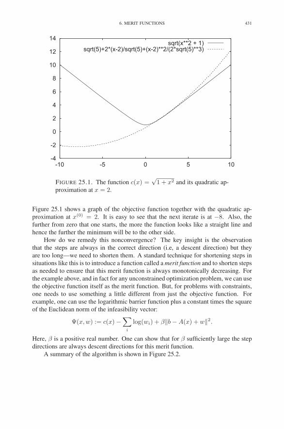
6. MERIT FUNCTIONS 431
-4
-2
0
2
4
6
8
10
12
14
-10 -5 0 5 10
sqrt(x**2 + 1)sqrt(5)+2*(x-2)/sqrt(5)+(x-2)**2/(2*sqrt(5)**3)
FIGURE 25.1. The function c(x) =√
1 + x2 and its quadratic ap-
proximation at x = 2.
Figure 25.1 shows a graph of the objective function together with the quadratic ap-
proximation at x(0) = 2. It is easy to see that the next iterate is at −8. Also, the
further from zero that one starts, the more the function looks like a straight line and
hence the further the minimum will be to the other side.
How do we remedy this nonconvergence? The key insight is the observation
that the steps are always in the correct direction (i.e, a descent direction) but they
are too long—we need to shorten them. A standard technique for shortening steps in
situations like this is to introduce a function called a merit function and to shorten steps
as needed to ensure that this merit function is always monotonically decreasing. For
the example above, and in fact for any unconstrained optimization problem, we can use
the objective function itself as the merit function. But, for problems with constraints,
one needs to use something a little different from just the objective function. For
example, one can use the logarithmic barrier function plus a constant times the square
of the Euclidean norm of the infeasibility vector:
Ψ(x,w) := c(x) −∑
i
log(wi) + β‖b − A(x) + w‖2.
Here, β is a positive real number. One can show that for β sufficiently large the step
directions are always descent directions for this merit function.
A summary of the algorithm is shown in Figure 25.2.
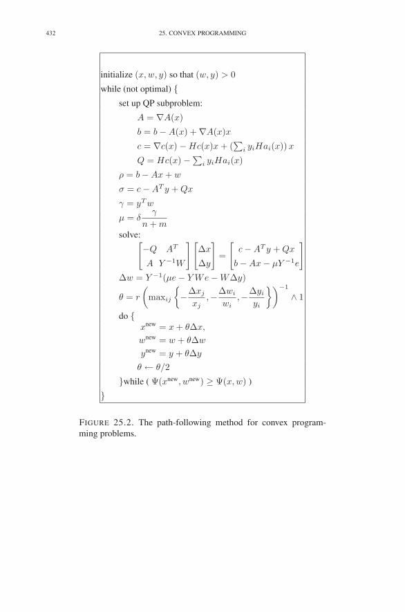
432 25. CONVEX PROGRAMMING
initialize (x,w, y) so that (w, y) > 0
while (not optimal) {set up QP subproblem:
A = ∇A(x)
b = b − A(x) + ∇A(x)x
c = ∇c(x) − Hc(x)x + (∑
i yiHai(x)) x
Q = Hc(x) −∑
i yiHai(x)
ρ = b − Ax + w
σ = c − AT y + Qx
γ = yT w
μ = δγ
n + msolve:
[
−Q AT
A Y −1W
][
∆x
∆y
]
=
[
c − AT y + Qx
b − Ax − μY −1e
]
∆w = Y −1(μe − Y We − W∆y)
θ = r
(
maxij
{
−∆xj
xj,−∆wi
wi,−∆yi
yi
})−1
∧ 1
do {xnew = x + θ∆x,
wnew = w + θ∆w
ynew = y + θ∆y
θ ← θ/2
}while ( Ψ(xnew, wnew) ≥ Ψ(x,w) )
}
FIGURE 25.2. The path-following method for convex program-
ming problems.

EXERCISES 433
7. Parting Words
A story is never over, but every book must have an end. So, we stop here mindful
of the fact that there are many interesting things left unsaid and topics unexplored. We
hope we have motivated the reader to pursue the story further without our assistance—
by reading other books and/or research papers and even perhaps making his or her own
contributions. Cheers.
Exercises
25.1 Piecewise Linear Approximation. Given real numbers b1 < b2 < · · · < bk,
let f be a continuous function on R that is linear on each interval [bi, bi+1],i = 0, 1, . . . , k (for convenience we let b0 = −∞ and bk+1 = ∞). Such a
function is called piecewise linear and the numbers bi are called breakpoints.
Piecewise linear functions are often used to approximate (continuous) non-
linear functions. The purpose of this exercise is to show how and why.
(a) Every piecewise linear function can be written as a sum of a constant
plus a linear term plus a sum of absolute value terms:
f(x) = d + a0x +
k∑
i=1
ai|x − bi|.
Let ci denote the slope of f on the interval [bi, bi+1]. Derive an explicit
expression for each of the aj’s (including a0) in terms of the ci’s.
(b) In terms of the ci’s, give necessary and sufficient conditions for f to be
convex.
(c) In terms of the aj’s, give necessary and sufficient conditions for f to be
convex.
(d) Assuming that f is convex and is a term in the objective function for
a linearly constrained optimization problem, derive an equivalent lin-
ear programming formulation involving at most k extra variables and
constraints.
(e) Repeat the first four parts of this problem using max(x− bi, 0) in place
of |x − bi|.25.2 Let f be the function of 2 real variables defined by
f(x, y) = x2 − 2xy + y2.
Show that f is convex.
25.3 A function f of 2 real variables is called a monomial if it has the form
f(x, y) = xmyn
for some nonnegative integers m and n. Which monomials are convex?
434 25. CONVEX PROGRAMMING
25.4 Let φ be a convex function of a single real variable. Let f be a function
defined on Rn by the formula
f(x) = φ(aT x + b),
where a is an n-vector and b is a scalar. Show that f is convex.
25.5 Which of the following functions are convex (assume that the domain of the
function is all of Rn unless specified otherwise)?
(a) 4x2 − 12xy + 9y2
(b) x2 + 2xy + y2
(c) x2y2
(d) x2 − y2
(e) ex−y
(f) ex2−y2
(g) x2
y on {(x, y) : y > 0}
25.6 Given a symmetric square matrix A, the quadratic form xT Ax =∑
i,j aijxixj
generalizes the notion of the square of a variable. The generalization of the
notion of the fourth power of a variable is an expression of the form
f(x) =∑
i,j,k,l
aijklxixjxkxl.
The four-dimensional array of numbers A = {aijkl : 1 ≤ i ≤ n, 1 ≤j ≤ n, 1 ≤ k ≤ n, 1 ≤ l ≤ n} is called a 4-tensor. As with quadratic
expressions, we may assume that A is symmetric:
aijkl = ajkli = · · · = alkij
(i.e., given i, j, k, l, all 4! = 24 premutations must give the same value for
the tensor).
(a) Give conditions on the 4-tensor A to guarantee that f is convex.
(b) Suppose that some variables, say yi’s, are related to some other vari-
ables, say xj’s, in a linear fashion:
yi =∑
j
fijxj .
Express∑
i y4i in terms of the xj’s. In particular, give an explicit ex-
pression for the 4-tensor and show that it satisfies the conditions derived
in part (a).
25.7 Consider the problem
minimize ax1 + x2
subject to√
ǫ2 + x21 ≤ x2.
NOTES 435
where −1 < a < 1.
(a) Graph the feasible set:{
(x1, x2) :√
ǫ2 + x21 ≤ x2
}
. Is the problem
convex?
(b) Following the steps in the middle of p. 391 of the text, write down the
first-order optimality conditions for the barrier problem associated with
barrier parameter μ > 0.
(c) Solve explicitly the first-order optimality conditions. Let (x1(μ), x2(μ))denote the solution.
(d) Graph the central path, (x1(μ), x2(μ)), as μ varies from 0 to ∞.
25.8 Multidimensional Taylor’s series expansion. Given a function g(t) defined
for real values of t, the three-term Taylor’s series expansion with remainder
is
g(t + ∆t) = g(t) + g′(t)∆t +1
2g′′(t)∆t2 + rt(∆t).
The remainder term satisfies
lim∆t→0
rt(∆t)
∆t2= 0.
Let f be a smooth function defined on Rn. Apply the three-term Taylor’s
series expansion to g(t) = f(x + t∆x) to show that
f(x + ∆x) = f(x) + ∇f(x)T ∆x +1
2∆xT Hf(x)∆x + rx(∆x).
25.9 Consider the following convex programming problem:
minimize x2
subject to x21 + x2
2 ≤ 1.
(a) Find the quadratic subproblem if the current primal solution is (x1, x2) =(1/2,−2/3) and the current dual solution is y = 2.
(b) Show that for arbitrary current primal and dual solutions, the feasible
set for the convex programming problem is contained within the feasi-
ble set for the quadratic approximation.
Notes
Interior-point methods for nonlinear programming can be traced back to the pio-
neering work of Fiacco & McCormick (1968). For more on interior-point methods for
convex programming, see Nesterov & Nemirovsky (1993) or den Hertog (1994).
The fact that the step directions are descent directions for the merit function Ψ is
proved in Vanderbei & Shanno (1999).

APPENDIX A
Source Listings
The algorithms presented in this book have all been implemented and are publicly
available from the author’s web site:
http://www.princeton.edu/˜rvdb/LPbook/
There are two variants of the simplex method: the two-phase method as shown
in Figure 6.1 and the self-dual method as shown in Figure 7.1. The simplex codes
require software for efficiently solving basis systems. There are two options: the eta-
matrix approach described in Section 8.3 and the refactorization approach described in
Section 8.5. Each of these “engines” can be used with either simplex method. Hence,
there are in total four possible simplex codes that one can experiment with.
There are three variants of interior-point methods: the path-following method as
shown in Figure 18.1, the homogeneous self-dual method shown in Figure 22.1 (mod-
ified to take long steps), and the long-step homogeneous self-dual method described
in Exercise 22.4 of Chapter 22.
The source code that implements the algorithms mentioned above share as much
common code as possible. For example, they all share the same input and output
routines (the input routine, by itself, is a substantial piece of code). They also share
code for the common linear algebra functions. Therefore, the difference between two
methods is limited primarily to the specific function that implements the method itself.
The total number of lines of code used to implement all of the algorithms is about
9000. That is too many lines to reproduce all of the code here. But the routines that
actually lay out the particular algorithms are fairly short, only about 300 lines each.
The relevant part of the self-dual simplex method is shown starting on the next page.
It is followed by a listing of the relevant part of the homogeneous self-dual method.
437
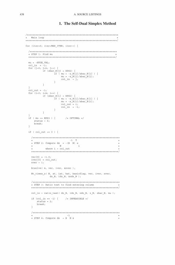
438 A. SOURCE LISTINGS
1. The Self-Dual Simplex Method
/***************************************************************** Main loop *****************************************************************/
for (iter=0; iter<MAX_ITER; iter++) {
/************************************************************** STEP 1: Find mu **************************************************************/
mu = -HUGE_VAL;col_in = -1;for (j=0; j<n; j++) {
if (zbar_N[j] > EPS2) {if ( mu < -z_N[j]/zbar_N[j] ) {
mu = -z_N[j]/zbar_N[j];col_in = j;
}}
}col_out = -1;for (i=0; i<m; i++) {
if (xbar_B[i] > EPS2) {if ( mu < -x_B[i]/xbar_B[i] ) {
mu = -x_B[i]/xbar_B[i];col_out = i;col_in = -1;
}}
}if ( mu <= EPS3 ) { /* OPTIMAL */
status = 0;break;
}
if ( col_out >= 0 ) {
/************************************************************** -1 T ** STEP 2: Compute dz = -(B N) e ** N i ** where i = col_out **************************************************************/
vec[0] = -1.0;ivec[0] = col_out;nvec = 1;
btsolve( m, vec, ivec, &nvec );
Nt_times_z( N, at, iat, kat, basicflag, vec, ivec, nvec,dz_N, idz_N, &ndz_N );
/************************************************************** STEP 3: Ratio test to find entering column **************************************************************/
col_in = ratio_test( dz_N, idz_N, ndz_N, z_N, zbar_N, mu );
if (col_in == -1) { /* INFEASIBLE */status = 2;break;
}
/************************************************************** -1 ** STEP 4: Compute dx = B N e *
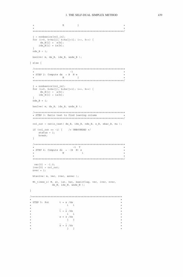
1. THE SELF-DUAL SIMPLEX METHOD 439
* B j ** **************************************************************/
j = nonbasics[col_in];for (i=0, k=ka[j]; k<ka[j+1]; i++, k++) {
dx_B[i] = a[k];idx_B[i] = ia[k];
}ndx_B = i;
bsolve( m, dx_B, idx_B, &ndx_B );
} else {
/************************************************************** -1 ** STEP 2: Compute dx = B N e ** B j **************************************************************/
j = nonbasics[col_in];for (i=0, k=ka[j]; k<ka[j+1]; i++, k++) {
dx_B[i] = a[k];idx_B[i] = ia[k];
}ndx_B = i;
bsolve( m, dx_B, idx_B, &ndx_B );
/************************************************************** STEP 3: Ratio test to find leaving column **************************************************************/
col_out = ratio_test( dx_B, idx_B, ndx_B, x_B, xbar_B, mu );
if (col_out == -1) { /* UNBOUNDED */status = 1;break;
}
/************************************************************** -1 T ** STEP 4: Compute dz = -(B N) e ** N i ** **************************************************************/
vec[0] = -1.0;ivec[0] = col_out;nvec = 1;
btsolve( m, vec, ivec, &nvec );
Nt_times_z( N, at, iat, kat, basicflag, vec, ivec, nvec,dz_N, idz_N, &ndz_N );
}
/************************************************************** ** STEP 5: Put t = x /dx ** i i ** _ _ ** t = x /dx ** i i ** s = z /dz ** j j ** _ _ ** s = z /dz ** j j *

440 A. SOURCE LISTINGS
*************************************************************/
for (k=0; k<ndx_B; k++) if (idx_B[k] == col_out) break;
t = x_B[col_out]/dx_B[k];tbar = xbar_B[col_out]/dx_B[k];
for (k=0; k<ndz_N; k++) if (idz_N[k] == col_in) break;
s = z_N[col_in]/dz_N[k];sbar = zbar_N[col_in]/dz_N[k];
/************************************************************** _ _ _ ** STEP 7: Set z = z - s dz z = z - s dz ** N N N N N N ** _ _ ** z = s z = s ** i i ** _ _ _ ** x = x - t dx x = x - t dx ** B B B B B B ** _ _ ** x = t x = t ** j j **************************************************************/
for (k=0; k<ndz_N; k++) {j = idz_N[k];z_N[j] -= s *dz_N[k];zbar_N[j] -= sbar*dz_N[k];
}
z_N[col_in] = s;zbar_N[col_in] = sbar;
for (k=0; k<ndx_B; k++) {i = idx_B[k];x_B[i] -= t *dx_B[k];xbar_B[i] -= tbar*dx_B[k];
}
x_B[col_out] = t;xbar_B[col_out] = tbar;
/************************************************************** STEP 8: Update basis **************************************************************/
i = basics[col_out];j = nonbasics[col_in];basics[col_out] = j;nonbasics[col_in] = i;basicflag[i] = -col_in-1;basicflag[j] = col_out;
/************************************************************** STEP 9: Refactor basis and print statistics **************************************************************/
from_scratch = refactor( m, ka, ia, a, basics, col_out, v );
if (from_scratch) {primal_obj = sdotprod(c,x_B,basics,m) + f;printf("%8d %14.7e %9.2e \n", iter, primal_obj, mu );fflush(stdout);
}}

2. THE HOMOGENEOUS SELF-DUAL METHOD 441
2. The Homogeneous Self-Dual Method
/***************************************************************** Main loop *****************************************************************/
for (iter=0; iter<MAX_ITER; iter++) {
/************************************************************** STEP 1: Compute mu and centering parameter delta.
*************************************************************/
mu = (dotprod(z,x,n)+dotprod(w,y,m)+phi*psi) / (n+m+1);
if (iter%2 == 0) {delta = 0.0;
} else {delta = 1.0;
}
/************************************************************** STEP 1: Compute primal and dual objective function values.
*************************************************************/
primal_obj = dotprod(c,x,n);dual_obj = dotprod(b,y,m);
/************************************************************** STEP 2: Check stopping rule.
*************************************************************/
if ( mu < EPS ) {if ( phi > EPS ) {
status = 0;break; /* OPTIMAL */
}elseif ( dual_obj < 0.0) {
status = 2;break; /* PRIMAL INFEASIBLE */
}elseif ( primal_obj > 0.0) {
status = 4;break; /* DUAL INFEASIBLE */
}else{
status = 7; /* NUMERICAL TROUBLE */break;
}}
/************************************************************** STEP 3: Compute infeasibilities.
*************************************************************/
smx(m,n,A,kA,iA,x,rho);for (i=0; i<m; i++) {
rho[i] = rho[i] - b[i]*phi + w[i];}normr = sqrt( dotprod(rho,rho,m) )/phi;for (i=0; i<m; i++) {
rho[i] = -(1-delta)*rho[i] + w[i] - delta*mu/y[i];}
smx(n,m,At,kAt,iAt,y,sigma);for (j=0; j<n; j++) {
sigma[j] = -sigma[j] + c[j]*phi + z[j];}

442 A. SOURCE LISTINGS
norms = sqrt( dotprod(sigma,sigma,n) )/phi;for (j=0; j<n; j++) {
sigma[j] = -(1-delta)*sigma[j] + z[j] - delta*mu/x[j];}
gamma = -(1-delta)*(dual_obj - primal_obj + psi) + psi - delta*mu/phi;
/************************************************************** Print statistics.
*************************************************************/
printf("%8d %14.7e %8.1e %14.7e %8.1e %8.1e \n",iter, primal_obj/phi+f, normr,
dual_obj/phi+f, norms, mu );fflush(stdout);
/************************************************************** STEP 4: Compute step directions.
*************************************************************/
for (j=0; j<n; j++) { D[j] = z[j]/x[j]; }for (i=0; i<m; i++) { E[i] = w[i]/y[i]; }
ldltfac(n, m, kAt, iAt, At, E, D, kA, iA, A, v);
for (j=0; j<n; j++) { fx[j] = -sigma[j]; }for (i=0; i<m; i++) { fy[i] = rho[i]; }
forwardbackward(E, D, fy, fx);
for (j=0; j<n; j++) { gx[j] = -c[j]; }for (i=0; i<m; i++) { gy[i] = -b[i]; }
forwardbackward(E, D, gy, gx);
dphi = (dotprod(c,fx,n)-dotprod(b,fy,m)+gamma)/(dotprod(c,gx,n)-dotprod(b,gy,m)-psi/phi);
for (j=0; j<n; j++) { dx[j] = fx[j] - gx[j]*dphi; }for (i=0; i<m; i++) { dy[i] = fy[i] - gy[i]*dphi; }
for (j=0; j<n; j++) { dz[j] = delta*mu/x[j] - z[j] - D[j]*dx[j]; }for (i=0; i<m; i++) { dw[i] = delta*mu/y[i] - w[i] - E[i]*dy[i]; }dpsi = delta*mu/phi - psi - (psi/phi)*dphi;
/************************************************************** STEP 5: Compute step length (long steps).
*************************************************************/
theta = 0.0;for (j=0; j<n; j++) {
if (theta < -dx[j]/x[j]) { theta = -dx[j]/x[j]; }if (theta < -dz[j]/z[j]) { theta = -dz[j]/z[j]; }
}for (i=0; i<m; i++) {
if (theta < -dy[i]/y[i]) { theta = -dy[i]/y[i]; }if (theta < -dw[i]/w[i]) { theta = -dw[i]/w[i]; }
}theta = MIN( 0.95/theta, 1.0 );
/************************************************************** STEP 6: Step to new point
*************************************************************/
for (j=0; j<n; j++) {x[j] = x[j] + theta*dx[j];z[j] = z[j] + theta*dz[j];
}for (i=0; i<m; i++) {
y[i] = y[i] + theta*dy[i];w[i] = w[i] + theta*dw[i];

2. THE HOMOGENEOUS SELF-DUAL METHOD 443
}phi = phi + theta*dphi;psi = psi + theta*dpsi;
}

Answers to Selected Exercises
1.3: See Exercise 2.19.
2.1: (x1, x2, x3, x4) = (2, 0, 1, 0), ζ = 17.
2.2: (x1, x2) = (1, 0), ζ = 2.
2.3: (x1, x2, x3) = (0, 0.5, 1.5), ζ = −3.
2.4: (x1, x2, x3) = (0, 1, 0), ζ = −3.
2.5: (x1, x2) = (2, 1), ζ = 5.
2.6: Infeasible.
2.7: Unbounded.
2.8: (x1, x2) = (4, 8), ζ = 28.
2.9: (x1, x2, x3) = (1.5, 2.5, 0), ζ = 10.5.
2.10: (x1, x2, x3, x4) = (0, 0, 0, 1), ζ = 9.
2.11: (x12, x13, x14, x23, x24, x34) = (1, 0, 0, 1, 0, 1), ζ = 6.
7.1: (1) x∗ = (2, 4, 0, 0, 0, 0, 8), ξ∗ = 14. (2) x∗ unchanged, ξ∗ = 12.2. (3)
x∗ = (0, 8, 0, 0, 0, 10, 10), ξ∗ = 16.
7.2: ∆c1 ∈ (−∞, 1.2], ∆c2 ∈ [−1.2,∞), ∆c3 ∈ [−1, 9], ∆c4 ∈ (−∞, 2.8].9.1: (x1, x2) = (0, 5).9.2: (x1, x2, x3, x4, x5, x6, x7, x8) = (0, 6, 1, 15, 2, 1, 0, 0).10.5: The fundamental theorem was proved only for problems in standard
form. The LP here can be reduced to standard form.
11.1: A should hide a or b with probabilities b/(a + b) and a/(a + b), respec-
tively. B should hide a or b with equal probability.
11.3:[
2 −4
−3 6
]
12.1: Slope = 2/7, intercept = 1.
12.2: Slope = 1/2, intercept = 0.
12.7: (2) 340. (3) x∗ is chosen so that the number of months in which extra
workers will be used is equal to the number of months in the cycle (12) times
the inhouse employee cost ($17.50) divided by the outhouse employee cost
($25) rounded down to the nearest integer.
12.8: Using L1, g = 8.976. With L2, g = 8.924.
445
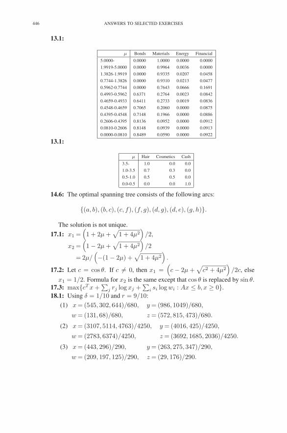
446 ANSWERS TO SELECTED EXERCISES
13.1:
μ Bonds Materials Energy Financial
5.0000- 0.0000 1.0000 0.0000 0.0000
1.9919-5.0000 0.0000 0.9964 0.0036 0.0000
1.3826-1.9919 0.0000 0.9335 0.0207 0.0458
0.7744-1.3826 0.0000 0.9310 0.0213 0.0477
0.5962-0.7744 0.0000 0.7643 0.0666 0.1691
0.4993-0.5962 0.6371 0.2764 0.0023 0.0842
0.4659-0.4933 0.6411 0.2733 0.0019 0.0836
0.4548-0.4659 0.7065 0.2060 0.0000 0.0875
0.4395-0.4548 0.7148 0.1966 0.0000 0.0886
0.2606-0.4395 0.8136 0.0952 0.0000 0.0912
0.0810-0.2606 0.8148 0.0939 0.0000 0.0913
0.0000-0.0810 0.8489 0.0590 0.0000 0.0922
13.1:
μ Hair Cosmetics Cash
3.5- 1.0 0.0 0.0
1.0-3.5 0.7 0.3 0.0
0.5-1.0 0.5 0.5 0.0
0.0-0.5 0.0 0.0 1.0
14.6: The optimal spanning tree consists of the following arcs:
{(a, b), (b, c), (c, f), (f, g), (d, g), (d, e), (g, h)}.
The solution is not unique.
17.1: x1 =(
1 + 2μ +√
1 + 4μ2)
/2,
x2 =(
1 − 2μ +√
1 + 4μ2)
/2
= 2μ/(
−(1 − 2μ) +√
1 + 4μ2)
.
17.2: Let c = cos θ. If c �= 0, then x1 =(
c − 2μ +√
c2 + 4μ2)
/2c, else
x1 = 1/2. Formula for x2 is the same except that cos θ is replaced by sin θ.
17.3: max{cT x +∑
j rj log xj +∑
i si log wi : Ax ≤ b, x ≥ 0}.
18.1: Using δ = 1/10 and r = 9/10:
(1) x = (545, 302, 644)/680, y = (986, 1049)/680,
w = (131, 68)/680, z = (572, 815, 473)/680.
(2) x = (3107, 5114, 4763)/4250, y = (4016, 425)/4250,
w = (2783, 6374)/4250, z = (3692, 1685, 2036)/4250.
(3) x = (443, 296)/290, y = (263, 275, 347)/290,
w = (209, 197, 125)/290, z = (29, 176)/290.
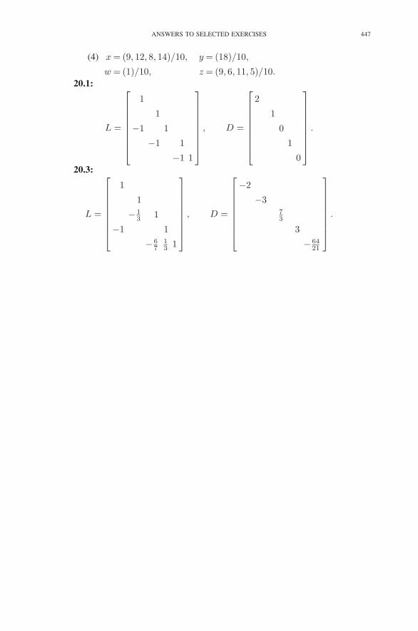
ANSWERS TO SELECTED EXERCISES 447
(4) x = (9, 12, 8, 14)/10, y = (18)/10,
w = (1)/10, z = (9, 6, 11, 5)/10.
20.1:
L =
⎡
⎢
⎢
⎢
⎢
⎢
⎢
⎢
⎣
1
1
−1 1
−1 1
−1 1
⎤
⎥
⎥
⎥
⎥
⎥
⎥
⎥
⎦
, D =
⎡
⎢
⎢
⎢
⎢
⎢
⎢
⎢
⎣
2
1
0
1
0
⎤
⎥
⎥
⎥
⎥
⎥
⎥
⎥
⎦
.
20.3:
L =
⎡
⎢
⎢
⎢
⎢
⎢
⎢
⎢
⎣
1
1
− 13 1
−1 1
− 67
13 1
⎤
⎥
⎥
⎥
⎥
⎥
⎥
⎥
⎦
, D =
⎡
⎢
⎢
⎢
⎢
⎢
⎢
⎢
⎣
−2
−373
3
− 6421
⎤
⎥
⎥
⎥
⎥
⎥
⎥
⎥
⎦
.

Bibliography
Adler, I. & Berenguer, S. (1981), Random linear programs, Technical Report 81-4,
Operations Research Center Report, U.C. Berkeley.
Adler, I., Karmarkar, N., Resende, M. & Veiga, G. (1989), ‘An implementation of Kar-
markar’s algorithm for linear programming’, Mathematical Programming 44, 297–
335.
Adler, I. & Megiddo, N. (1985), ‘A simplex algorithm whose average number of steps
is bounded between two quadratic functions of the smaller dimension’, Journal of
the ACM 32, 871–895.
Ahuja, R., Magnanti, T. & Orlin, J. (1993), Network Flows: Theory, Algorithms, and
Applications, Prentice Hall, Englewood Cliffs, NJ.
Anstreicher, K. (1996), Potential Reduction Algorithms, Technical report, Department
of Management Sciences, University of Iowa.
Barnes, E. (1986), ‘A variation on Karmarkar’s algorithm for solving linear program-
ming problems’, Mathematical Programming 36, 174–182.
Bayer, D. & Lagarias, J. (1989a), ‘The nonlinear geometry of linear programming. I.
affine and projective scaling trajectories’, Transactions of the AMS 314, 499–525.
Bayer, D. & Lagarias, J. (1989b), ‘The nonlinear geometry of linear programming. II.
Legendre transform coordinates and central trajectories’, Transactions of the AMS
314, 527–581.
Bazaraa, M., Jarvis, J. & Sherali, H. (1977), Linear Programming and Network Flows,
2 edn, Wiley, New York.
Bellman, R. (1957), Dynamic Programming, Princeton University Press, Princeton,
NJ.
Bendsøe, M., Ben-Tal, A. & Zowe, J. (1994), ‘Optimization methods for truss geom-
etry and topology design’, Structural Optimization 7, 141–159.
Bertsekas, D. (1991), Linear Network Optimization, The MIT Press, Cambridge, MA.
Bertsekas, D. (1995), Nonlinear Programming, Athena Scientific, Belmont MA.
Bland, R. (1977), ‘New finite pivoting rules for the simplex method’, Mathematics of
Operations Research 2, 103–107.
Bloomfield, P. & Steiger, W. (1983), Least Absolute Deviations: Theory, Applications,
and Algorithms, Birkhauser, Boston.
449

450 Bibliography
Borgwardt, K.-H. (1982), ‘The average number of pivot steps required by the simplex-
method is polynomial’, Zeitschrift fur Operations Research 26, 157–177.
Borgwardt, K.-H. (1987a), Probabilistic analysis of the simplex method, in ‘Opera-
tions Research Proceedings, 16th DGOR Meeting’, pp. 564–576.
Borgwardt, K.-H. (1987b), The Simplex Method—A Probabilistic Approach, Springer-
Verlag, Berlin-Heidelberg-New York.
Bradley, S., Hax, A. & Magnanti, T. (1977), Applied Mathematical Programming,
Addison Wesley, Reading, MA.
Caratheodory, C. (1907), ‘Uber den Variabilitatsbereich der Koeffizienten von Poten-
zreihen, die gegebene Werte nicht annehmen’, Mathematische Annalen 64, 95–115.
Carpenter, T., Lustig, I., Mulvey, J. & Shanno, D. (1993), ‘Higher order predictor-
corrector interior point methods with application to quadratic objectives’, SIAM
Journal on Optimization 3, 696–725.
Charnes, A. (1952), ‘Optimality and degeneracy in linear programming’, Economet-
rica 20, 160–170.
Christofides, N. (1975), Graph Theory: An Algorithmic Approach, Academic Press,
New York.
Chvatal, V. (1983), Linear Programming, Freeman, New York.
Dantzig, G. (1951a), Application of the simplex method to a transportation problem,
in T. Koopmans, ed., ‘Activity Analysis of Production and Allocation’, John Wiley
and Sons, New York, pp. 359–373.
Dantzig, G. (1951b), A proof of the equivalence of the programming problem and the
game problem, in T. Koopmans, ed., ‘Activity Analysis of Production and Alloca-
tion’, John Wiley and Sons, New York, pp. 330–335.
Dantzig, G. (1955), ‘Upper bounds, secondary constraints, and block triangularity in
linear programming’, Econometrica 23, 174–183.
Dantzig, G. (1963), Linear Programming and Extensions, Princeton University Press,
Princeton, NJ.
Dantzig, G. & Orchard-Hayes, W. (1954), ‘The product form for the inverse in the
simplex method’, Mathematical Tables and Other Aids to Computation 8, 64–67.
Dantzig, G., Orden, A. & Wolfe, P. (1955), ‘The generalized simplex method for
minimizing a linear form under linear inequality constraints’, Pacific Journal of
Mathematics 5, 183–195.
den Hertog, D. (1994), Interior Point Approach to Linear, Quadratic, and Convex
Programming, Kluwer Academic Publishers, Dordrecht.
Dijkstra, E. (1959), ‘A note on two problems in connexion with graphs’, Numerische
Mathematik 1, 269–271.
Dikin, I. (1967), ‘Iterative solution of problems of linear and quadratic programming’,
Soviet Mathematics Doklady 8, 674–675.
Dikin, I. (1974), ‘On the speed of an iterative process’, Upravlyaemye Sistemi 12, 54–
60.

Bibliography 451
Dodge, Y., ed. (1987), Statistical Data Analysis Based on The L1-Norm and Related
Methods, North-Holland, Amsterdam.
Dorn, W., Gomory, R. & Greenberg, H. (1964), ‘Automatic design of optimal struc-
tures’, J. de Mecanique 3, 25–52.
Dresher, M. (1961), Games of Strategy: Theory and Application, Prentice-Hall, En-
glewood Cliffs, NJ.
Duff, I., Erisman, A. & Reid, J. (1986), Direct Methods for Sparse Matrices, Oxford
University Press, Oxford.
Elias, P., Feinstein, A. & Shannon, C. (1956), ‘Note on maximum flow through a
network’, IRE Transactions on Information Theory IT-2, 117–119.
Farkas, J. (1902), ‘Theorie der einfachen Ungleichungen’, Journal fur die reine und
angewandte Mathematik 124, 1–27.
Fiacco, A. & McCormick, G. (1968), Nonlinear Programming: Sequential Uncon-
strainted Minimization Techniques, Research Analysis Corporation, McLean Vir-
ginia. Republished in 1990 by SIAM, Philadelphia.
Ford, L. & Fulkerson, D. (1956), ‘Maximal flow through a network’, Canadian Jour-
nal of Mathematics 8, 399–404.
Ford, L. & Fulkerson, D. (1958), ‘Constructing maximal dynamic flows from static
flows’, Operations Research 6, 419–433.
Ford, L. & Fulkerson, D. (1962), Flows in Networks, Princeton University Press,
Princeton, NJ.
Forrest, J. & Tomlin, J. (1972), ‘Updating triangular factors of the basis to maintain
sparsity in the product form simplex method’, Mathematical Programming 2, 263–
278.
Fourer, R., Gay, D. & Kernighan, B. (1993), AMPL: A Modeling Language for Math-
ematical Programming, Scientific Press.
Fourer, R. & Mehrotra, S. (1991), ‘Solving symmetric indefinite systems in an interior
point method for linear programming’, Mathematical Programming 62, 15–40.
Fulkerson, D. & Dantzig, G. (1955), ‘Computation of maximum flow in networks’,
Naval Research Logistics Quarterly 2, 277–283.
Gal, T., ed. (1993), Degeneracy in Optimization Problems, Vol. 46/47 of Annals of
Operations Research, J.C. Baltzer AG.
Gale, D., Kuhn, H. & Tucker, A. (1951), Linear programming and the theory of games,
in T. Koopmans, ed., ‘Activity Analysis of Production and Allocation’, John Wiley
and Sons, New York, pp. 317–329.
Garey, M. & Johnson, D. (1977), Computers and Intractability, W.H. Freeman and
Company, San Francisco.
Garfinkel, R. & Nemhauser, G. (1972), Integer Programming, John Wiley and Sons,
New York.
Gass, S. & Saaty, T. (1955), ‘The computational algorithm for the parametric objective
function’, Naval Research Logistics Quarterly 2, 39–45.

452 Bibliography
Gay, D. (1985), ‘Electronic mail distribution of linear programming test problems’,
Mathematical Programming Society COAL Newslettter 13, 10–12.
Gill, P., Murray, W., Ponceleon, D. & Saunders, M. (1992), ‘Preconditioners for in-
definite systems arising in optimization’, SIAM Journal on Matrix Analysis and
Applications 13(1), 292–311.
Gill, P., Murray, W. & Wright, M. (1991), Numerical Linear Algebra and Optimiza-
tion, Vol. 1, Addison-Wesley, Redwood City, CA.
Goldfarb, D. & Reid, J. (1977), ‘A practicable steepest-edge simplex algorithm’,
Mathematical Programming 12, 361–371.
Golub, G. & VanLoan, C. (1989), Matrix Computations, 2 edn, The Johns Hopkins
University Press, Baltimore, MD.
Gonin, R. & Money, A. (1989), Nonlinear Lp-Norm Estimation, Marcel Dekker, New
York-Basel.
Gordan, P. (1873), ‘Uber die Auflosung linearer Gleichungen mit reelen Coefficien-
ten’, Mathematische Annalen 6, 23–28.
Hall, L. & Vanderbei, R. (1993), ‘Two-thirds is sharp for affine scaling’, OR Letters
13, 197–201.
Harris, P. (1973), ‘Pivot selection methods of the Devex LP code’, Mathematical Pro-
gramming 5, 1–28.
Hemp, W. (1973), Optimum Structures, Clarendon Press, Oxford.
Hillier, F. & Lieberman, G. (1977), Introduction to Mathematical Programming, 2
edn, McGraw-Hill, New York.
Hitchcock, F. (1941), ‘The distribution of a produce from several sources to numerous
localities’, Journal of Mathematical Physics 20, 224–230.
Hoffman, A. (1953), Cycling in the simplex algorithm, Technical Report 2974,
National Bureau of Standards.
Howard, R. (1960), Dynamic Programming and Markov Processes, John Wiley and
Sons, New York.
Huard, P. (1967), Resolution of mathematical programming with nonlinear constraints
by the method of centers, in J. Abadie, ed., ‘Nonlinear Programming’, North-
Holland, Amsterdam, pp. 209–219.
Jensen, P. & Barnes, J. (1980), Network Flow Programming, John Wiley and Sons,
New York.
John, F. (1948), Extremum problems with inequalities as subsidiary conditions, in
K. Fredrichs, O. Neugebauer & J. Stoker, eds, ‘Studies and Essays: Courant An-
niversary Volume’, Wiley Interscience, New York, pp. 187–204.
Kantorovich, L. (1960), ‘Mathematical methods in the organization and planning of
production’, Management Science 6, 550–559. Original Russian version appeared
in 1939.
Karlin, S. (1959), Mathematical Methods and Theory in Games, Programming, and
Economics, Vol. 1 and 2, Addison-Wesley, Reading, MA.

Bibliography 453
Karmarkar, N. (1984), ‘A new polynomial time algorithm for linear programming’,
Combinatorica 4, 373–395.
Karush, W. (1939), Minima of functions of several variables with inequalities as side
conditions, Technical report, M.S. Thesis, Department of Mathematics, University
of Chicago.
Kennington, J. & Helgason, R. (1980), Algorithms for Network Programming, John
Wiley and Sons, New York.
Khachian, L. (1979), ‘A polynomial algorithm in linear programming’, Doklady
Academiia Nauk SSSR 244, 191–194. In Russian. English Translation: Soviet Math-
ematics Doklady 20: 191-194.
Klee, V. & Minty, G. (1972), How good is the simplex algorithm?, in O. Shisha, ed.,
‘Inequalities–III’, Academic Press, New York, pp. 159–175.
Kojima, M., Mizuno, S. & Yoshise, A. (1989), A primal-dual interior point algorithm
for linear programming, in N. Megiddo, ed., ‘Progress in Mathematical Program-
ming’, Springer-Verlag, New York, pp. 29–47.
Kotzig, A. (1956), Suvislost’ a Pravidelina Suvislots’ Konecnych Grafov, Technical
report, Bratislava: Vysoka Skola Ekonomicka.
Kuhn, H. (1950), ‘A simplified two-person poker’, Annals of Mathematics Studies
24, 97–103.
Kuhn, H. (1976), Nonlinear prgramming: A historical view, in R. Cottle & C. Lemke,
eds, ‘Nonlinear Programming, SIAM-AMS Proceedings’, Vol. 9, American Math-
etical Society, Providence, RI, pp. 1–26.
Kuhn, H. & Tucker, A. (1951), Nonlinear prgramming, in J. Neyman, ed., ‘Proceed-
ings of the Second Berkeley Symposium on Mathematical Statistics and Probabil-
ity’, University of California Press, Berkeley, CA, pp. 481–492.
Lawler, E. (1976), Combinatorial Optimization: Networks and Matroids, Holt, Rine-
hart and Winston, New York.
Lemke, C. (1954), ‘The dual method of solving the linear programming problem’,
Naval Research Logistics Quarterly 1, 36–47.
Lemke, C. (1965), ‘Bimatrix equilibrium points and mathematical programming’,
Management Science 11, 681–689.
Luenberger, D. (1984), Introduction to Linear and Nonlinear Programming, Addison-
Wesley, Reading MA.
Lustig, I. (1990), ‘Feasibility issues in a primal-dual interior-point method for linear
programming’, Mathematical Programming 49(2), 145–162.
Lustig, I., Marsten, R. & Shanno, D. (1994), ‘Interior point methods for linear pro-
gramming: computational state of the art’, ORSA J. on Computing 6, 1–14.
Markowitz, H. (1957), ‘The elimination form of the inverse and its application to linear
programming’, Management Science 3, 255–269.
Markowitz, H. (1959), Portfolio Selection: Efficient Diversification of Investments,
Wiley, New York.

454 Bibliography
Marshall, K. & Suurballe, J. (1969), ‘A note on cycling in the simplex method’, Naval
Research Logistics Quarterly 16, 121–137.
Mascarenhas, W. (1997), ‘The affine scaling algorithm fails for λ = 0.999’, SIAM J.
Optimization 7, 34–46.
Megiddo, N. (1989), Pathways to the optimal set in linear programming, in
N. Megiddo, ed., ‘Progress in Mathematical Programming’, Springer-Verlag, New
York, pp. 131–158.
Mehrotra, S. (1989), Higher order methods and their performance, Technical Report
TR 90-16R1, Department of Ind. Eng. and Mgmt. Sci., Northwestern University,
Evanston, IL. Revised July, 1991.
Mehrotra, S. (1992), ‘On the implementation of a (primal-dual) interior point method’,
SIAM Journal on Optimization 2, 575–601.
Michell, A. (1904), ‘The limits of economy of material in frame structures’, Phil. Mag.
8, 589–597.
Mizuno, S., Todd, M. & Ye, Y. (1993), ‘On adaptive-step primal-dual interior-point
algorithms for linear programming’, Mathematics of Operations Research 18, 964–
981.
Monteiro, R. & Adler, I. (1989), ‘Interior path following primal-dual algorithms: Part
i: Linear programming’, Mathematical Programming 44, 27–41.
Nash, S. & Sofer, A. (1996), Linear and Nonlinear Programming, McGraw-Hill, New
York.
Nazareth, J. (1986), ‘Homotopy techniques in linear programming’, Algorithmica
1, 529–535.
Nazareth, J. (1987), Computer Solutions of Linear Programs, Oxford University Press,
Oxford.
Nazareth, J. (1996), ‘The implementation of linear programming algorithms based on
homotopies’, Algorithmica 15, 332–350.
Nemhauser, G. & Wolsey, L. (1988), Integer and Combinatorial Optimization, Wiley,
New York.
Nesterov, Y. & Nemirovsky, A. (1993), Interior Point Polynomial Methods in Convex
Programming : Theory and Algorithms, SIAM Publications, Philadelphia.
Recski, A. (1989), Matroid Theory and its Applications in Electric Network Theory
and in Statics, Springer-Verlag, Berlin-Heidelberg-New York.
Reid, J. (1982), ‘A sparsity-exploiting variant of the Bartels-Golub decomposition for
linear programming bases’, Mathematical Programming 24, 55–69.
Rockafellar, R. (1970), Convex Analysis, Princeton University Press, Princeton, NJ.
Rozvany, G. (1989), Structural Design via Optimality Criteria, Kluwer, Dordrecht.
Ruszczynski, A. & Vanderbei, R. (2003), Frontiers of Stochastically Nondominated
Portfolios’, Econometrica 71(4), 1287–1297.
Saigal, R. (1995), Linear Programming, Kluwer Academic Publishers, Boston.
Bibliography 455
Saunders, M. (1973), The complexity of LU updating in the simplex method, in R. An-
dersen & R. Brent, eds, ‘The complexity of computational problem solving’, Uni-
versity Press, Queensland, pp. 214–230.
Smale, S. (1983), ‘On the average number of steps of the simplex method of linear
programming’, Mathematical Programming 27, 241–262.
Stiemke, E. (1915), ‘Uber positive Losungen homogener linearer Gleichungen’, Math-
ematische Annalen 76, 340–342.
Todd, M. (1986), ‘Polynomial expected behavior of a pivoting algorithm for linear
complementarity and linear programming’, Mathematical Programming 35, 173–
192.
Todd, M. (1995), Potential-reduction methods in mathematical programming, Techni-
cal Report 1112, SORIE, Cornell University, Ithaca, NY.
Tsuchiya, T. & Muramatsu, M. (1992), ‘Global convergence of a long-step affine scal-
ing algorithm for degenerate linear programming problems’, SIAM J. Optimization
5(3), 525–551.
Tucker, A. (1956), ‘Dual systems of homogeneous linear equations’, Annals of Math-
ematics Studies 38, 3–18.
Turner, K. (1991), ‘Computing projections for the Karmarkar algorithm’, Linear Al-
gebra and Its Applications 152, 141–154.
Vanderbei, R. (1989), ‘Affine scaling for linear programs with free variables’, Mathe-
matical Programming 43, 31–44.
Vanderbei, R. (1994), ‘Interior-point methods: algorithms and formulations’, ORSA J.
on Computing 6, 32–34.
Vanderbei, R. (1995), ‘Symmetric quasi-definite matrices’, SIAM Journal on Opti-
mization 5(1), 100–113.
Vanderbei, R. (1999), ‘LOQO: An interior point code for quadratic programming’,
Optimization Methods and Software 12, 451–484.
Vanderbei, R. & Carpenter, T. (1993), ‘Symmetric indefinite systems for interior-point
methods’, Mathematical Programming 58, 1–32.
Vanderbei, R., Meketon, M. & Freedman, B. (1986), ‘A modification of Karmarkar’s
linear programming algorithm’, Algorithmica 1, 395–407.
Vanderbei, R. & Shanno, D. (1999), An Interior-Point Algorithm for Nonconvex
Nonlinear Programming’, Computational Optimization and Applications 13, 231–
252.
Ville, J. (1938), Sur la theorie general des jeux ou intervient l’habilete des jouers,
in E. Borel, ed., ‘Traite du Calcul des Probabilites et des ses Applications’, Paris,
Gauthiers-Villars.
von Neumann, J. (1928), ‘Zur Theorie der Gesselschaftschpiele’, Mathematische An-
nalen 100, 295–320.
von Neumann, J. & Morgenstern, O. (1947), Theory of Games and Economic Behav-
ior, 2nd edn, Princeton University Press, Princeton, NJ.
Wright, S. (1996), Primal-Dual Interior-Point Methods, SIAM, Philadelphia, USA.

456 Bibliography
Xu, X., Hung, P. & Ye, Y. (1993), A simplified homogeneous and self-dual linear pro-
gramming algorithm and its implementation, Technical report, College of Business
Administration, University of Iowa. To appear in Annals of Operations Research.
Ye, Y., Todd, M. & Mizuno, S. (1994), ‘An o(√
nl)-iteration homogeneous and self-
dual linear programming algorithm’, Mathematics of Operations Research 19, 53–
67.

Index
LDLT -factorization, 330
LU -factorization, 128
L2-regression, 193
Lp-norm, 193
Acyclic network, 229
Adler & Berenguer (1981), 209, 449
Adler & Megiddo (1985), 53, 208, 449
Adler et al. (1989), 381, 449
Affine-scaling algorithm, 345
Ahuja et al. (1993), 252, 269, 449
Algorithm
affine-scaling, 345
Dijkstra’s, 258
dual simplex, 103
homogeneous, self-dual interior-point, 376
parametric self-dual simplex, 121
path-following, 308
convex programming, 432
general form, 343
quadratic programming, 419
primal simplex, 103
self-dual network simplex, 241
self-dual parametric simplex, 124
successive quadratic programming, 429
Anstreicher (1996), 318, 449
arbitrage, 220
Arc, 225
head of, 229
Ascent direction, 345
Assignment problem, 255
Auxiliary problem, 19
Axes, pitch, roll, and yaw, 279
Backward substitution, 130
Balanced flow, 230
Barnes (1986), 358, 449
Barrier function, 290
Barrier problem, 289, 290
Basic feasible solution, 16
Basic variables, 16
Bayer & Lagarias (1989a), 301, 449
Bayer & Lagarias (1989b), 301, 449
Bazaraa et al. (1977), 11, 252, 449
Bellman (1957), 269, 449
Bellman’s equation, 257
Ben-Tal, A., xvi
Bendsøe et al. (1994), 284, 449
Bernstein, D.H., xvi
Bertsekas (1991), 252, 449
Bertsekas (1995), 301, 423, 449
Bimatrix games, 185
Bipartite graph, 253
Bland (1977), 44, 449
Bland’s rule, 36
Bloomfield & Steiger (1983), 208, 449
Bluffing, 181
Borgwardt (1982), 53, 124, 208, 449
Borgwardt (1987a), 53, 208, 450
Borgwardt (1987b), 53, 450
Bradley et al. (1977), 11, 450
Branch-and-bound, 385, 392
Breadth-first search, 395
Bump, 142
Capacity
cut, 262
Caratheodory (1907), 171, 450
Carpenter et al. (1993), 318, 450
Central path, 289, 292, 299
Centroid, 204
Certificate of optimality, 66
457

458 INDEX
Charnes (1952), 44, 450
Christofides (1975), 252, 450
Chvatal (1983), 27, 187, 450
Cınlar, E., xvi
Column dominance, 185
Come-from, 388
Complementarity, 296
strict, 168
Complementary slackness theorem, 66
Complexity
predictor-corrector algorithm, 371
Complexity theory, 54
Concave function, 170, 426
Connected, 229, 249
Connected components, 249
Conservation laws, 276
Continuous paths, 354
Convergence, 308, 353, 369
Convex analysis, 161
Convex combination, 161
Convex function, 423, 426
Convex hull, 163
Convex programming, 425
interior-point method for, 427
Convex quadratic programming problem, 416
Convex set, 161
Corrector step, 366
Cost
lost opportunity, 5
Crew scheduling problem, 386
Critical point, 191
Critical points, 292
Cut set, 262
Cycle, 229
Cycling, 30
Dantzig (1951a), 10, 252, 450
Dantzig (1951b), 10, 450
Dantzig (1955), 160, 450
Dantzig (1963), 10, 27, 124, 450
Dantzig & Orchard-Hayes (1954), 150, 450
Dantzig et al. (1955), 44, 450
Dantzig, G.B., 10, 27, 87
Dantzig, T., 87
Decision variables, 6
Degeneracy, 29
geometry, 39
Degenerate dictionary, 29
Degenerate pivot, 29
Demand node, 253
den Hertog (1994), 435, 450
Depth-first search, 395
Destination node, 253
Devex, 150
Dictionary, 16
Diet problem, 85
Digraph, 225
Dijkstra (1959), 269, 450
Dijkstra’s algorithm, 258
Dikin (1967), 358, 450
Dikin (1974), 358, 450
Directed paths, 256
Dodge (1987), 208, 450
Dorn et al. (1964), 284, 451
Dresher (1961), 187, 451
Dual estimates, 358
Dual network simplex method, 237
Dual pivot, 239, 242
Dual problem, 57
general form, 73
Dual simplex method, 68, 101, 153, 155
Duality Theory, 55
Duff et al. (1986), 150, 451
Dynamic programming, 257
Edge, 40
Efficiency
simplex method, 45, 198
Efficient frontier, 216, 411
Elias et al. (1956), 269, 451
Ellipsoid method, 54
Entering arc, 242
Entering variable, 17, 94, 102
Enumeration tree, 395
Equilibrium
Nash, 185
Equivalence classes, 249
Equivalence relation, 249
Eta matrix, 140
Eta-file, 140
Facet, 40
Facility location, 204
Factorization
LDLT , 330
LU , 128
instability and quasidefinite matrices, 334
stability and positive definite matrices, 330
Fair game, 178
Farkas’ lemma, 167

INDEX 459
Farkas (1902), 171, 451
Feasible flow, 230
Feasible solution, 7
Fiacco & McCormick (1968), 301, 435, 451
Fixed costs, 390
Flow balance constraints, 227
Folven, G., xvi
Ford & Fulkerson (1956), 269, 451
Ford & Fulkerson (1958), 252, 451
Ford & Fulkerson (1962), 252, 451
Forrest & Tomlin (1972), 150, 451
Forward substitution, 129
Fourer & Mehrotra (1991), 344, 451
Fourer et al. (1993), xiv, 451
Fourer, R., xiv
Fourier, 10
Fulkerson & Dantzig (1955), 269, 451
Function
barrier, 290
concave, 170, 426
strongly, 86
convex, 423, 426
strongly, 86
objective, 6
Gal (1993), 44, 451
Gale et al. (1951), 87, 187, 451
Game Theory, 173
Games
bimatrix, 185
zero-sum, 173
Garey & Johnson (1977), 54, 451
Garfinkel & Nemhauser (1972), 405, 451
Garfinkel, R.S., xvi
Gass & Saaty (1955), 124, 451
Gay (1985), 199, 451
Gay, D.M., xiv
Gill et al. (1991), 150, 452
Gill et al. (1992), 344, 452
Gilmartin, J., xvi
Go-to, 388
Goldfarb & Reid (1977), 150, 452
Golub & VanLoan (1989), 150, 452
Gonin & Money (1989), 208, 452
Gordan (1873), 171, 452
Gradient, 425
Graph, 225
Gravity, acceleration due to, 206
Gross, L., xvi
Holder’s inequality, 311
Halfspace, 40, 165
generalized, 165
Hall & Vanderbei (1993), 358, 452
Hall, L.A., xvi
Harris (1973), 150, 452
Hedging, 212
Hemp (1973), 284, 452
Hessian, 294, 425
Higher-order methods, 316
Hillier & Lieberman (1977), 11, 452
Hitchcock (1941), 269, 452
Hitchcock transportation problem, 254
Hoffman (1953), 43, 452
Homogeneous problem, 362, 363
Homogeneous self-dual method, 361
Homotopy method, 115, 315
Howard (1960), 269, 452
Huard (1967), 301, 452
Ikura, Y., xvi
Incidence matrix, 274
Infeasibility, 8, 157, 304
Infeasible dictionary, 20
Initialization
dual-based, 71
Integer programming, 243
Integer programming problem, 385, 392
Integrality theorem, 243
Interior-point methods, 289
affine-scaling, 345
homogeneous, self-dual, 376
path-following, 308
convex programming, 432
general form, 343
quadratic programming, 419
Inventory, cost of, 4
Iterative reweighted least squares, 207
Iteratively reweighted least squares, 196
Jensen & Barnes (1980), 252, 452
John (1948), 325, 452
Joint, 271
Konig’s Theorem, 244
Kantorovich (1960), 10, 452
Karlin (1959), 187, 452
Karmarkar, N.K., 318
Karmarkar (1984), 301, 318, 358, 453
Karush, W., 319, 325, 342, 418
Karush–Kuhn–Tucker (KKT) system, 319

460 INDEX
Karush-Kuhn-Tucker (KKT) system, 372
Karush (1939), 325, 453
Kennington & Helgason (1980), 252, 453
Kernighan, B., xiv
Khachian (1979), 54, 318, 453
Klee & Minty (1972), 53, 453
Klee, V., xvi
Knapsack problem, 404
Kojima et al. (1989), 318, 453
Koopmans, T.C., 10
Kotzig (1956), 269, 453
Kuhn (1950), 187, 453
Kuhn (1976), 325, 453
Kuhn & Tucker (1951), 325, 453
Kuhn, H.W., 319, 342, 418
Label-correcting algorithm, 257
Label-setting algorithm, 257
Labels, 257
Lagrange multipliers, 292, 293
Lagrangian, 294
Lagrangian duality, 78
Lawler (1976), 252, 453
Least squares, 194
Leaving arc, 242
Leaving variable, 17, 95, 102
Legendre transform, 87
Legs, 385
Lemke (1954), 87, 453
Lemke (1965), 124, 453
Lemma
Farkas’, 167
Lexicographic method, 32, 35, 44
Linear complementarity problem, 186, 316
Linear program
standard form, 7
Logarithmic barrier function, 290
Long-step method, 379, 380
Lower bounds, 151
LP-relaxation, 256, 393
Luenberger (1984), 301, 453
Lustig (1990), 318, 453
Lustig et al. (1994), 342, 453
Lustig, I.J., xvi
Mandelbaum, A., xvi
Markowitz (1957), 150, 453
Markowitz (1959), 222, 423, 453
Markowitz model, 407
Marshall & Suurballe (1969), 43, 453
Mascarenhas (1997), 358, 454
Matrix
notation, 89
positive definite, 327
quasidefinite, 331
sparse, 130
Matrix game, 173
Maximum-flow problem, 262
Mean, 189
Median, 190
Mediocrity, measures thereof, 189
Megiddo (1989), 301, 454
Mehrotra (1989), 380, 454
Mehrotra (1992), 380, 454
Meketon, M.S., xvi
Member, 271
Method
affine-scaling, 345
dual network simplex, 237
dual simplex, 68, 101, 103, 153
higher-order, 316
homogeneous self-dual, 361
homogeneous, self-dual interior-point, 376
homotopy, 315
lexicographic, 32
long-step, 379, 380
Newton’s, 305
out-of-kilter, 252
parametric self-dual simplex, xviii
parametric self-dual simplex, 118, 119, 121
path-following, 289, 303, 308
convex programming, 432
general form, 343
quadratic programming, 419
perturbation, 32
predictor-corrector, 366
primal network simplex, 233
primal simplex, 91, 103, 151
primal–dual simplex, xviii, 118
self-dual network simplex, 241
self-dual parametric simplex, 124
short-step, 380
simplex, 13
two phase, 104
Michell (1904), 284, 454
Midrange, 203
Minimum Operator ∧, 307
Minimum-cost network flow problem, 225
Minimum-degree ordering, 130

INDEX 461
Minimum-weight structural design problem,
279
Mixed integer programming problem, 404
Mizuno et al. (1993), 380, 454
Moment arm, 277
Monteiro & Adler (1989), 318, 423, 454
Nabona, N., xvi
Nash & Sofer (1996), 301, 423, 454
Nash equilibrium, 185
Nazareth (1986), 124, 318, 454
Nazareth (1987), 124, 454
Nazareth (1996), 318, 454
Negative transpose, 61
Nemhauser & Wolsey (1988), 405, 454
Nesterov & Nemirovsky (1993), 435, 454
Network, 225
acyclic, 229
complete, 251
connected, 229
Network flow problems, 225
Network simplex method, 252
Newton’s method, 305
Node, 225
Node-arc incidence matrix, 228
Nonbasic variables, 16
Nonlinear objective function, 390
Nonlinear programming, 301
Normal equations, 320, 321
Null space, 348
Null variable, 169
Objective function, 6
Onion skin, 354
Optimal solution, 7
Optimality
check for, 93, 102
Optimality conditions
first-order, 294–296, 339, 413, 414, 418, 427
Option Pricing, 216
Orden, A., 43
Orlin, J.B., xvi
Orthogonal projection, 348
Out-of-Kilter method, 252
Parametric analysis, 115
Parametric self-dual simplex method, 118, 119
Partial pricing, 147
Path, 228
Path-following method, 289, 303
Penalty function, 422
Perturbation method, 32, 43
Phase I, 22
dual-based, 71
Phase II, 22
piecewise linear function, 433
Pivot, 19
Pivot rule, 19
Planar network, 250
Poker, 181
Polyhedron, 40, 165
Polynomial complexity, 53
Portfolio optimization, 211, 407
Portfolio selection, 211
Positive definite matrix, 327
Positive semidefinite matrix, 324, 416
closure under summation, 324
closure under inversion, 324
Predictor step, 366
Predictor-Corrector Algorithm, 366
Predictor-corrector algorithm
complexity, 371
Primal flow, 228
Primal network simplex method, 233
Primal pivot, 233, 242
Primal problem, 57
Primal scaling, 357
Primal simplex method, 91, 151
Primal–dual network simplex method, 252
Primal–dual scaling, 357
Primal–dual simplex method, 118
Principle stresses, 282
Probability
of infeasibility, 87
of unboundedness, 87
Problem
assignment, 202, 255
auxiliary, 19
barrier, 289, 290
convex quadratic programming, 416
crew scheduling, 386
diet, 85
dual, 57
equipment scheduling, 386
Hitchcock transportation, 254
homogeneous linear programming, 363
homogeneous self-dual, 362
integer programming, 385, 392
knapsack, 404
linear complementarity, 186, 316

462 INDEX
linear programming
general form, 151, 337
maximum-flow, 262
minimum-cost network, 225
minimum-weight structural design, 279
mixed integer programming, 404
network flow, 225
network flows, 225
primal, 57
quadratic penalty, 422
quadratic programming, 407
scheduling, 385
self-dual linear programming, 363
separable quadratic programming, 420
set-covering, 386
set-partitioning, 386
shortest path, 256
transportation, 253
transshipment, 253
traveling salesman, 387
upper-bounded network flow, 259
Programming
nonlinear, 301
Projected gradient direction, 347
scaled, 349
Projection, 348
Projective geometry, 301
Pruning, 403
quadratic form, 434
Quadratic penalty problem, 422
Quadratic programming problem, 407
convex, 414
dual, 412
interior-point method for, 418
Quasidefinite matrix, 331
Ranges, 151
Recski (1989), 284, 454
Reduced KKT system, 320, 372, 418
Regression, 189
Regression model, 192
Reid (1982), 150, 454
Resource allocation, 4, 74
Revised simplex method, 109
Reward, 211, 408
Risk, 211, 408
Rockafellar (1970), 171, 454
Root
of a function, 305
Root node, 231, 256
Roses, 109
Route, 385
Row dominance, 185
Row operations, 14
Rozvany (1989), 284, 454
Ruszczynski & Vanderbei (2003), 222, 454
Ruszczynski, A., xvi
Saddle points, 86
Saigal (1995), 359, 454
Sailing, 281
Sales force planning, 205
Saunders (1973), 150, 454
Scale invariance, 315
Scaling matrices, 357
Scheduling problem, 385
Second-order conditions, 297
Self-dual linear program, 363
Self-dual parametric simplex method, 124
Self-dual problem, 362
Self-dual simplex method, 118
Sensitivity analysis, 111
Separable quadratic programming problem, 420
Separation theorem, 165
Set-covering problem, 386
Set-partitioning problem, 386
Sherman–Morrison–Woodbury formula, 325
Short-step method, 380
Shortest-path problem, 256
Simplex method
primal–dual, xviii
Simplex method, 13
dual, 103
geometry, 22
initialization, 19
dual-based, 71
parametric self-dual, xviii, 121
primal, 103
revised, 109
self-dual network, 241
unboundedness, 22
worst-case analysis, 47
Sink node, 262
Skew symmetric matrix, 275
Slack variable, 7, 13
Smale (1983), 53, 124, 208, 455
Solution, 7
basic feasible, 16
feasible, 7

INDEX 463
optimal, 7
tree, 230
Source node, 253, 262
Spanning tree, 229
Sparse matrix, 130
Sparsity, 130
Spike column, 142
Stability, 274
Stable structure, 276
Steepest ascent, 346
Steepest edge, 147
Steiner tree, 205
Step direction, 94, 305
affine-scaling, 351
dual, 95, 102
primal, 102
Step direction decomposition, 324
Step length, 94, 95, 102
Stiemke (1915), 171, 455
Stochastic vector, 175
Strategy
randomized, 175
Strict complementarity, 168
Strictly positive vector, 298
Strictly positive vector (>), 168
Strong duality theorem, 60
Strongly convex function, 86
Strongly concave function, 86
Structural optimization, 271
Subnetwork, 229
Substitution
backward, 130
forward, 129
Successive approximations, 258
Successive quadratic programming algorithm,
429
Supply node, 253
Supremum norm, 309
Symmetric games, 178
Tableau
simplex, 27
Tail of an arc, 229
Taylor’s series, 435
tensor, 434
Theorem
ascent direction, 323
Bland’s rule, 36
Caratheodory, 164
central path, 298
complementary slackness, 67
convergence of affine-scaling, 353
convergence of simplex method, 32
convex hull, 163
efficiency of interior-point method, 312
integrality, 243
Konig, 244
lexicographic rule, 35
linear programming, fundamental, 38
local maximum, 294
max-flow min-cut, 263
minimax, 178
optimality for convex quadratic programs,
416
separating hyperplane, 165
spanning tree, 231
strict complementary slackness, 169
strong duality, 60
weak duality, 58
Todd (1986), 53, 208, 455
Todd (1995), 318, 455
Todd, M.J., xvi
Topology, 271
Transportation problem, 253
Transshipment problem, 253
Traveling salesman problem, 387
Tree, 229
solution, 230
spanning, 229
Triangle inequality, 368
Truss, 280
Tsuchiya & Muramatsu (1992), 358, 455
Tucker (1956), 171, 380, 455
Tucker, A.W., 319, 342, 418
Turner (1991), 344, 455
Two-phase methods, 104
Unboundedness, 8, 22
Underbidding, 181
Unitary matrix, 278
Upper bounds, 151
Upper-bounded network flow problem, 259
Value, 178
Value function, 257
Vanderbei (1989), 359, 455
Vanderbei (1994), 344, 455
Vanderbei (1995), 344, 455
Vanderbei (1999), 423, 455

464 INDEX
Vanderbei & Carpenter (1993), 344, 455
Vanderbei & Shanno (1999), 435, 455
Vanderbei et al. (1986), 358, 455
Variable
basic, 16
decision, 6
entering, 17, 94, 102
leaving, 17, 95, 102
nonbasic, 16
null, 169
slack, 7, 13
Vector norms, 309
Vehicle routing, 404
Vertex, 40
Ville (1938), 171, 455
von Neumann (1928), 187, 455
von Neumann & Morgenstern (1947), 187,
455
von Neumann, J., 87
Warnie, J., xvi
Weak duality theorem, 58
Wolkowicz, H., xvi
Woolbert, S., xvi
Worst-case analysis, 47
Wright (1996), 318, 455
Wu, L., xvi
Xu et al. (1993), 380, 455
Yang, B., xvi
Ye et al. (1994), 380, 456

Early Titles in the
INTERNATIONAL SERIES IN
OPERATIONS RESEARCH & MANAGEMENT SCIENCE Frederick S. Hillier, Series Editor, Stanford University
Saigal/ A MODERN APPROACH TO LINEAR PROGRAMMING Nagurney/ PROJECTED DYNAMICAL SYSTEMS & VARIATIONAL INEQUALITIES WITH
APPLICATIONS
Padberg & Rijal/ LOCATION, SCHEDULING, DESIGN AND INTEGER PROGRAMMING
Vanderbei/ LINEAR PROGRAMMING Jaiswal/ MILITARY OPERATIONS RESEARCH Gal & Greenberg/ ADVANCES IN SENSITIVITY ANALYSIS & PARAMETRIC PROGRAMMING Prabhu/ FOUNDATIONS OF QUEUEING THEORY Fang, Rajasekera & Tsao/ ENTROPY OPTIMIZATION & MATHEMATICAL PROGRAMMING Yu/ OR IN THE AIRLINE INDUSTRY Ho & Tang/ PRODUCT VARIETY MANAGEMENT El-Taha & Stidham/ SAMPLE-PATH ANALYSIS OF QUEUEING SYSTEMS Miettinen/ NONLINEAR MULTIOBJECTIVE OPTIMIZATION Chao & Huntington/ DESIGNING COMPETITIVE ELECTRICITY MARKETS Weglarz/ PROJECT SCHEDULING: RECENT TRENDS & RESULTS Sahin & Polatoglu/ QUALITY, WARRANTY AND PREVENTIVE MAINTENANCE
Tavares/ ADVANCES MODELS FOR PROJECT MANAGEMENT Tayur, Ganeshan & Magazine/ QUANTITATIVE MODELS FOR SUPPLY CHAIN MANAGEMENT Weyant, J./ ENERGY AND ENVIRONMENTAL POLICY MODELING
Shanthikumar, J.G. & Sumita, U./ APPLIED PROBABILITY AND STOCHASTIC PROCESSES
Liu, B. & Esogbue, A.O./ DECISION CRITERIA AND OPTIMAL INVENTORY PROCESSES
Gal, T., Stewart, T.J., Hanne, T. / MULTICRITERIA DECISION MAKING: Advances in MCDM Models, Algorithms, Theory, and Applications
Fox, B.L. / STRATEGIES FOR QUASI-MONTE CARLO
Hall, R.W. / HANDBOOK OF TRANSPORTATION SCIENCE
Grassman, W.K. / COMPUTATIONAL PROBABILITY
Pomerol, J-C. & Barba-Romero, S. / MULTICRITERION DECISION IN MANAGEMENT
Axsäter, S. / INVENTORY CONTROL
Wolkowicz, H., Saigal, R., & Vandenberghe, L. / HANDBOOK OF SEMI-DEFINITE PROGRAMMING: Theory, Algorithms, and Applications Hobbs, B.F. & Meier, P. / ENERGY DECISIONS AND THE ENVIRONMENT: A Guide
to the Use of Multicriteria Methods Dar-El, E. / HUMAN LEARNING: From Learning Curves to Learning Organizations Armstrong, J.S. / PRINCIPLES OF FORECASTING: A Handbook for Researchers and
Practitioners Balsamo, S., Personé, V., & Onvural, R./ ANALYSIS OF QUEUEING NETWORKS WITH BLOCKING Bouyssou, D. et al. / EVALUATION AND DECISION MODELS: A Critical Perspective Hanne, T. / INTELLIGENT STRATEGIES FOR META MULTIPLE CRITERIA DECISION MAKING Saaty, T. & Vargas, L. / MODELS, METHODS, CONCEPTS and APPLICATIONS OF THE ANALYTIC HIERARCHY PROCESS Chatterjee, K. & Samuelson, W. / GAME THEORY AND BUSINESS APPLICATIONS
Hobbs, B. et al. / THE NEXT GENERATION OF ELECTRIC POWER UNIT COMMITMENT MODELS Vanderbei, R.J. / LINEAR PROGRAMMING: Foundations and Extensions, 2nd Ed. Kimms, A. / MATHEMATICAL PROGRAMMING AND FINANCIAL OBJECTIVES FOR SCHEDULING PROJECTS
Baptiste, P., Le Pape, C. & Nuijten, W. / CONSTRAINT-BASED SCHEDULING

Early Titles in the
INTERNATIONAL SERIES IN
OPERATIONS RESEARCH & MANAGEMENT SCIENCE
(Continued)
Feinberg, E. & Shwartz, A. / HANDBOOK OF MARKOV DECISION PROCESSES: Methods
and Applications
Ramík, J. & Vlach, M. / GENERALIZED CONCAVITY IN FUZZY OPTIMIZATION
AND DECISION ANALYSIS
Song, J. & Yao, D. / SUPPLY CHAIN STRUCTURES: Coordination, Information and
Optimization
Kozan, E. & Ohuchi, A. / OPERATIONS RESEARCH/ MANAGEMENT SCIENCE AT WORK
Bouyssou et al. / AIDING DECISIONS WITH MULTIPLE CRITERIA: Essays in
Honor of Bernard Roy
Cox, Louis Anthony, Jr. / RISK ANALYSIS: Foundations, Models and Methods
Dror, M., L’Ecuyer, P. & Szidarovszky, F. / MODELING UNCERTAINTY: An Examination
of Stochastic Theory, Methods, and Applications
Dokuchaev, N. / DYNAMIC PORTFOLIO STRATEGIES: Quantitative Methods and Empirical Rules
for Incomplete Information
Sarker, R., Mohammadian, M. & Yao, X. / EVOLUTIONARY OPTIMIZATION
Demeulemeester, R. & Herroelen, W. / PROJECT SCHEDULING: A Research Handbook
Gazis, D.C. / TRAFFIC THEORY
Zhu/ QUANTITATIVE MODELS FOR PERFORMANCE EVALUATION AND BENCHMARKING
Ehrgott & Gandibleux/ MULTIPLE CRITERIA OPTIMIZATION: State of the Art Annotated Bibliographical
Surveys
Bienstock/ Potential Function Methods for Approx. Solving Linear Programming Problems
Matsatsinis & Siskos/ INTELLIGENT SUPPORT SYSTEMS FOR MARKETING
DECISIONS
Alpern & Gal/ THE THEORY OF SEARCH GAMES AND RENDEZVOUS
Hall/HANDBOOK OF TRANSPORTATION SCIENCE - 2nd Ed.
Glover & Kochenberger/ HANDBOOK OF METAHEURISTICS
Graves & Ringuest/ MODELS AND METHODS FOR PROJECT SELECTION:
Concepts from Management Science, Finance and Information Technology
Hassin & Haviv/ TO QUEUE OR NOT TO QUEUE: Equilibrium Behavior in Queueing Systems
Gershwin et al/ ANALYSIS & MODELING OF MANUFACTURING SYSTEMS
Maros/ COMPUTATIONAL TECHNIQUES OF THE SIMPLEX METHOD
Harrison, Lee & Neale/ THE PRACTICE OF SUPPLY CHAIN MANAGEMENT: Where Theory and
Application Converge
Shanthikumar, Yao & Zijm/ STOCHASTIC MODELING AND OPTIMIZATION OF
MANUFACTURING SYSTEMS AND SUPPLY CHAINS
Nabrzyski, Schopf & WĊglarz/ GRID RESOURCE MANAGEMENT: State of the Art and Future Trends
Thissen & Herder/ CRITICAL INFRASTRUCTURES: State of the Art in Research and Application
Carlsson, Fedrizzi, & Fullér/ FUZZY LOGIC IN MANAGEMENT
Soyer, Mazzuchi & Singpurwalla/ MATHEMATICAL RELIABILITY: An Expository Perspective
Chakravarty & Eliashberg/ MANAGING BUSINESS INTERFACES: Marketing, Engineering, and
Manufacturing Perspectives
Talluri & van Ryzin/ THE THEORY AND PRACTICE OF REVENUE MANAGEMENT
Kavadias & Loch/PROJECT SELECTION UNDER UNCERTAINTY: Dynamically Allocating Resources to
Maximize Value

Early Titles in the
INTERNATIONAL SERIES IN
OPERATIONS RESEARCH & MANAGEMENT SCIENCE (Continued)
Brandeau, Sainfort & Pierskalla/ OPERATIONS RESEARCH AND HEALTH CARE: A Handbook of
Methods and Applications
Cooper, Seiford & Zhu/ HANDBOOK OF DATA ENVELOPMENT ANALYSIS: Models and Methods
Luenberger/ LINEAR AND NONLINEAR PROGRAMMING, 2nd Ed.
Sherbrooke/ OPTIMAL INVENTORY MODELING OF SYSTEMS: Multi-Echelon Techniques,
Second Edition
Chu, Leung, Hui & Cheung/ 4th PARTY CYBER LOGISTICS FOR AIR CARGO
Simchi-Levi, Wu & Shen/ HANDBOOK OF QUANTITATIVE SUPPLY CHAIN ANALYSIS: Modeling
in the E-Business Era
Gass & Assad/ AN ANNOTATED TIMELINE OF OPERATIONS RESEARCH: An Informal History
Greenberg/ TUTORIALS ON EMERGING METHODOLOGIES AND APPLICATIONS IN OPERATIONS
RESEARCH
Weber/ UNCERTAINTY IN THE ELECTRIC POWER INDUSTRY: Methods and Models for Decision
Support
Figueira, Greco & Ehrgott/ MULTIPLE CRITERIA DECISION ANALYSIS: State of the Art Surveys
Reveliotis/ REAL-TIME MANAGEMENT OF RESOURCE ALLOCATIONS SYSTEMS: A Discrete Event
Systems Approach
Kall & Mayer/ STOCHASTIC LINEAR PROGRAMMING: Models, Theory, and Computation
* A list of the more recent publications in the series is at the front of the book *