forward scatter radar: innovative configurations and studies
TRANSCRIPT

FORWARD SCATTER RADAR:
INNOVATIVE CONFIGURATIONS AND STUDIES
by
Alessandro De Luca
A thesis submitted to the University of Birmingham for the degree of
DOCTOR OF PHILOSOPHY
Electronic, Electrical and System Engineering
University of Birmingham
February 2018

University of Birmingham Research Archive
e-theses repository This unpublished thesis/dissertation is copyright of the author and/or third parties. The intellectual property rights of the author or third parties in respect of this work are as defined by The Copyright Designs and Patents Act 1988 or as modified by any successor legislation. Any use made of information contained in this thesis/dissertation must be in accordance with that legislation and must be properly acknowledged. Further distribution or reproduction in any format is prohibited without the permission of the copyright holder.

Abstract
This thesis is dedicated to the study of innovative forward scatter radar (FSR) configurations
and techniques. FSR is a specific kind of bistatic radar characterized by a bistatic angle equal
or close to 180˚. Differently from other systems, this radar has not been deeply studied.
Therefore, many of its capabilities are still unknown. The goal of this PhD project is to
investigate techniques and configurations which would improve FSR performance, making it a
more appealing system. This thesis proposes an initial radar overview with deep focus on
forward scatter capabilities. FSR principles, radar cross section and target signature are widely
discussed. Thus, numerous innovative studies done during this PhD project are presented. FSR
passive mode, MIMO geometry and moving transmitter/ moving receiver configurations are
here investigated for the first time. For each of these subjects, numerous experimental
campaigns have been undertaken and a big quantity of data has been collected.
Comprehensive analyses on measured and simulated results are also presented. Moreover,
various novel techniques to estimate target motion parameters have been developed and
tested on real and simulated data. Results show a good match between measured and
estimated kinematic information. Finally, clutter in moving ends FSR is discussed. In fact, the
innovative configuration here presented, characterized by transmitter and/or receiver moving,
is affected by Doppler shift and clutter Doppler spread. Thus, it is important to understand how
this issue limits the system performance.

Acknowledgements
This PhD project has been successfully closed thanks to the effort of many people who helped
me during this incredible experience.
Firstly, I would like to express my gratitude to my mentors and supervisors Prof. Gashinova
and Prof. Cherniakov. Thank you for the guidance, knowledge and vision you have offered me.
Also, thanks for giving me the freedom to follow my instinct, to make mistakes and to learn.
Secondly, I would like to thank all the MISL group members for the fun and good time we had.
This environment has made my PhD experience much more enjoyable.
I would like to extend particular thanks to:
Liam, Stan, Dimitris and Micaela for inspiring, supporting and motivating me and for the nice
moments spent together.
To my girlfriend Marielle that has shared with me all the stressful moments and some of the
joyful ones. Thank you for all the time you have listened to me and motivated me.
Finally, I would like to dedicate this achievement to my family. To my mother, father and sister,
thanks for your endless love. I would have never been able to reach this goal without your life
time support.

Contents Acknowledgements .................................................................................................................... 3
Introduction ............................................................................................................... 1
1.1 Radar Overview ................................................................................................................ 1
1.2 Brief History of Radar ....................................................................................................... 4
1.3 Radar Basics ...................................................................................................................... 7
Monostatic Radar ...................................................................................................... 7
Bistatic Geometry .................................................................................................... 10
Radar Equation ........................................................................................................ 13
Radar Cross Section ................................................................................................. 15
1.4 PhD Research Focus ........................................................................................................ 16
Forward Scatter Radar State of the Art ................................................................... 16
PhD Project: Motivations and Innovative Work ...................................................... 17
Author Publications ................................................................................................. 20
1.5 Thesis Organization ........................................................................................................ 21
1.6 Bibliography .................................................................................................................... 23
Forward Scatter Radar Background ......................................................................... 27
2.1 Introduction .................................................................................................................... 27
2.2 Forward Scatter Radar .................................................................................................... 28
Forward Scatter Radar Geometry ........................................................................... 28
Forward Radar Cross Section ................................................................................... 30
Power Budget in FSR ................................................................................................ 37
Forward Scatter Radar Target Signature ................................................................. 43
Clutter in Forward Scatter Radar ............................................................................. 46
2.3 Radars on Moving Platforms .......................................................................................... 50
Ground Return Spectrum ........................................................................................ 50
2.4 Moving Ends Forward Scatter Radar .............................................................................. 53
2.5 Summary ......................................................................................................................... 55
2.6 Bibliography .................................................................................................................... 56
Target Signature and Parameter Estimation ........................................................... 59
3.1 Introduction .................................................................................................................... 59
3.2 Simulated Target Doppler Signature in Time Domain .................................................... 61
Influence of Transmitting and Target Parameters on the Doppler Signature ........ 62
3.3 Estimation of Target Motion Parameters in Time Domain ............................................ 67
3.4 Simulated Target Doppler Signature in Frequency Domain ........................................... 71
Influence of Transmitting and Target Parameters on the Doppler Signature’s
Spectrogram ..................................................................................................................... 72
3.5 Speed Estimation in Frequency Domain ........................................................................ 78
Experimental Results ............................................................................................... 81
3.6 Time and Frequency Domain Approaches in Difficult Scenarios ................................... 85
Small Target ............................................................................................................. 85
Big Target ................................................................................................................. 86
Cluttered Environment ............................................................................................ 88
3.7 Moving Transmitter/Moving Receiver Target Doppler Signature.................................. 89
3.8 Target Motion Parameter Estimation in Moving Tx/Moving Rx Scenario ..................... 91
Experimental Results ............................................................................................... 93
3.9 Conclusions ..................................................................................................................... 97
3.10 Bibliography .................................................................................................................. 99
Clutter in FSR ......................................................................................................... 100
4.1 Introduction .................................................................................................................. 100
4.2 Land Clutter .................................................................................................................. 102

4.3 Clutter Model................................................................................................................ 105
Simulated Surface .................................................................................................. 105
Simulated Vegetation ............................................................................................ 106
Doppler Signature Creation ................................................................................... 113
4.4 Clutter Measurements ................................................................................................. 117
4.5 Conclusions ................................................................................................................... 127
4.6 Bibliography .................................................................................................................. 129
Passive Forward Scatter Radar .............................................................................. 131
5.1 Introduction .................................................................................................................. 132
5.2 Target Doppler Signature Extraction ............................................................................ 133
5.3 Power Budget Analysis ................................................................................................. 137
FSCS Patterns ......................................................................................................... 137
Preliminary Power Budget ..................................................................................... 141
5.4 Experimental Measurements with Airliners ................................................................. 145
System Set Up ........................................................................................................ 145
Experimental Results ............................................................................................. 148
5.5 Experimental Measurements with Light and Ultralight Aircrafts ................................ 151
UoB Scenario and Results ...................................................................................... 151
5.6 Speed Estimation .......................................................................................................... 156
5.7 Passive FSR with Moving Receiver ............................................................................... 157
FHR Scenario and Results ...................................................................................... 157
Highly cluttered environment ............................................................................... 160
5.8 Conclusions ................................................................................................................... 167
5.9 Bibliography .................................................................................................................. 169
MIMO Forward Scatter Radar................................................................................ 171
6.1 Introduction .................................................................................................................. 171

6.2 MIMO Geometry .......................................................................................................... 173
Parameters Estimation Based on Multiple Baselines Crossing Times ................... 175
6.3 System Development .................................................................................................... 176
Equipment ............................................................................................................. 177
System Design ........................................................................................................ 178
Geometry ............................................................................................................... 181
Targets ................................................................................................................... 183
6.4 Experimental Results .................................................................................................... 185
Extraction of the Doppler Signature ...................................................................... 185
Experimental Results ............................................................................................. 187
6.5 Conclusions ................................................................................................................... 189
6.6 Bibliography .................................................................................................................. 191
Conclusions and Future Work................................................................................ 193
7.1 Summary ....................................................................................................................... 193
7.2 Conclusions ................................................................................................................... 196
7.3 Future work .................................................................................................................. 198
Appendix A: Target Doppler Signature Extraction ................................................................. 200
Appendix B: Maritime Cooperative Targets ........................................................................... 204
Appendix C: Maritime Equipment .......................................................................................... 208
Appendix D: Clutter Measurements Equipment .................................................................... 213
Appendix E: USRP 2950R ........................................................................................................ 221

Chapter 1: Introduction
1
Introduction
Glossary of Abbreviations
CH Chain Home
CW Continuous Wave
EM ElectroMagnetic
FSR Forward Scatter Radar
IF Intermediate Frequency
KH Klein Heildeberg
LoS Line of Sight
MIMO Multi Input Multi Output
OTH Over-The-Horizon
PRF Pulse Repetition Frequency
RADAR RAdio Detection and Ranging
RCS Radar Cross Section
RF Radio Frequency
Rx Receiver
SNR Signal to Noise Ratio
Tx Transmitter
UK United Kingdom
1.1 Radar Overview
RADAR, acronym of RAdio Detection and Ranging, is a system aiming to detect and locate
objects through the use of electromagnetic (EM) waves [1]. This is achieved by capturing the

Chapter 1: Introduction
2
interference of transmitted EM waves with physical objects present within the coverage area.
The received echo not only reveals the presence of a target, but it also carries some target-
related information, such as its speed, direction, trajectory and composition. Moreover, radar
presents some meaningful peculiarities making its use indispensable. In fact, this system offers
long and short distance coverage in all-weather and also low-visibility conditions, such as in
darkness, fog, haze [2].
A typical radar configuration includes a Transmitter (Tx) and a Receiver (Rx) side. The former
consists of a transmitter connected to an antenna. Tx generates an electric signal which is then
converted and radiated outwardly as electromagnetic wave by the transmit antenna.
Similarly, the latter is a combination of antenna and receiver. The antenna captures the EM
wave that is then converted into a received waveform. A processing of this waveform enables
the radar to detect the presence of a target and extract more information about it.
The way the transmitter and receiver are placed in the space determines principles and
features of a specific radar. Thus, radar systems can be classified in three different
configurations based on Tx and Rx topology: monostatic, bistatic and multistatic [1].
(a) (b)
(c)
Figure 1.1. Monostatic (a), bistatic (b) and multistatic radar (c) configuration.

Chapter 1: Introduction
3
Figure 1.1 shows these three different kinds of radar designs. When transmitter and receiver
are co-located, as in Figure 1.1 (a), the system is called monostatic radar [1], [3]. This system
is the most common type of radar and exploits the backscattering from the target. In other
words, the transmitted power reaches the target, whose distance from the Tx is equal to R ;
the scattering object reradiates the intercepted incident energy in different directions and the
receiver captures the portion incident on it [2], [4]. The amount of power density spread by
the target in the different directions depends on its radar cross section (RCS), further discussed
in the following pages. When Tx and Rx are separated by a significant fraction of the target
range the system is defined as bistatic radar [1], [3]. Figure 1.1 (b) shows its configuration. TxR
and RxR are the distances transmitter-target and target-receiver respectively, while is the
angle formed between Tx, target and Rx, known as bistatic angle [3], [5]. The radar concept
can be extended to a system of radars exploiting one or more transmitters and more than one
receiver [3], [6], as shown in Figure 1.1 (c). This configuration, called multistatic radar,
introduces several advantages whenever the information from all the stations is combined
together. In fact, it would be possible to cover a bigger area, have a higher performance in
target detection and localization and benefit power advantages. Obviously, some drawbacks
are introduced, mainly related to the need to process together data from different stations
[6].
Radar systems can also be distinguished according to the transmitted waveform: continuous
wave (CW) radars transmit continuously with either an unmodulated or a modulated
waveform; on the other hand, pulsed radars transmit a pulsed waveform.
In addition to what already said, radar can use a dedicated transmitter or transmitters of
opportunities. On the base of that, the system is defined as active, the former, or passive, the
latter.
This thesis focuses on CW forward scatter radar (FSR), a specific kind of bistatic radar, which
is largely described in Chapter 2, operating in both active and passive mode.

Chapter 1: Introduction
4
1.2 Brief History of Radar
The term radar was coined in 1940 by the U.S. Navy and made official by Admiral H. R. Stark,
who declared:
“The type of radio equipment which has been developed under Special Project No.1 which
has been referred to as “Radio Ranging Equipment”, “Radio Detection Equipment”, “Radio
Echo Equipment”, etc., will hereafter be known as “Radio Detection and Ranging
Equipment””.
However, the origins of this system date back to the last decades of the 19th century [7]. In
fact, between 1885 and 1888, the German physicist Heinrich Hertz demonstrated a parallelism
between radio waves and light, showing how the former could be reflected by metallic objects
[2], [7]. The same phenomenon was resumed by Nikola Tesla, who suggested the possibility
to determine the position of a moving object using reflected waves. However, it was Alexander
Popov, during the same period, to verify for the first time radar-based device detection
capabilities. In fact, in 1897, he reported the detection of the warship “Lieutenant Il’in” after
it crossed the radio communication link between two other ships [8], [9]. Popov, as well as
Hertz and Tesla, did not investigate further possible applications on the topic. The world was
not ready for such kind of system yet and even the patented and demonstrated by Christian
Hülsmeyer telemobilskop, known as the first radar device, able to detect ships up to 5 km from
the receiver, was rejected by several organizations and eventually forgotten [8]. In fact,
despite that period was quite difficult for the shipping market, the arrival of wireless
telegraphy made possible communications between ships at bigger distances. Therefore,
there was reluctance in spending money on a device not seen as necessary yet [8]. Due to the
lack of documentation and industry interest, radar was repetitively rediscovered and rejected
during the next following years.
In the late 1920s and early 1930s, due to the appearance of heavy military bomber aircrafts
and with the presage of an approaching war, a strong interest in radar raised again [2]. Thus,
simultaneously and independently several countries, such as United States, United Kingdom,
Soviet Union, Germany, Italy, France, Netherlands and Japan, started developing radar
systems. Most of the early radar prototypes were bistatic radars configured as fixed ground

Chapter 1: Introduction
5
based fences, using commercial radio transmitters and detecting targets crossing the line of
sight (LoS) between transmitter and receiver. Such kind of systems had the big inconvenience
of lack of target range estimation. Because of the political tension, boundary security was
extremely important and several of these electronic fences were installed along the countries’
borders. In France, multiple chain systems were configured; among all, the most complex was
the “maille en Z”, meaning “mesh in the shape of Z”. It was a system working at 30 MHz able
to estimate speed, direction and altitude of an aircraft with good accuracy [8]. In the Soviet
Union, a forward scatter fence named RUS-1 operating at 75 MHz went into production. In
Japan, the VHF fence Type A was able to detect crossing aircrafts with baseline over 650 km
[5], [8]. Also in the United Kingdom (UK), several tests culminated in the development of the
Chain Home (CH), an alarm system set along the English and Scottish coast extremely effective
against the Luftwaffe during World War II. It was a system working between 22-50 MHz. A
typical station comprised of three in line transmitter stations and four receiver towers, with
Tx and Rx sites separated for isolation. However, Chain Home radars had also a reversionary
mode, to be used in case of transmitter failure or electronic countermeasures, enabling a
receiver to operate with an adjacent transmitter site, located around 40 km away [5], [8]. In
response to the British Chain Home, the Germans developed the first bistatic radar using non-
cooperative transmitters, the Klein Heildeberg Parasit (KH) [5]. In fact, this was a system using
the British Chain Home as transmitter. However, while the UK CH was a result of a big defence
project, developed after a deep phase of tests and covering the whole coast facing Germany,
the German KH was a technology quickly built after the enemy chain was discovered.
Therefore, not much time was spent on tests and developments. In addition to that, the
system included only few receivers.
It is only after the invention of the duplexer in 1936 by the US Naval Research Laboratory
engineers, which allowed the use of a single antenna for both transmitter and receiver, that
monostatic pulsed radars became more practical, with consequent loss of interest in bistatic
radar after the World War II [6], [8]. Monostatic radar theory, technology and techniques,
together with measurements continued to develop after the end of the conflict with focus on
bistatic configurations going up and down at times.

Chapter 1: Introduction
6
An interest in redeveloping bistatic radar base on the improvements of monostatic arose in
the early 1950s, period in which the term “bistatic radar” was coined [5]. Bistatic and forward
scatter RCS theory was developed and experiments on this topic and on bistatic clutter were
taken. In the post-war years the United States invested significantly in defence technology,
due to the emerging international tension. They built and developed a system of FSR fences,
the Fluttar, operating in combination with other surveillance radars. However, too many false
alarms due to presence of birds and the impossibility to locate and track targets caused the
device’s dismissal. Later, over-the-horizon (OTH) radars were investigated with the aim to
detect nuclear weapons blasts and ballistic missile launches. In fact, different from typical
radars, OTH, using the reflections by the ionosphere, could perform at great distances,
detecting and identifying different kind of missiles based on the different signatures [5], [10].
For the same purpose, also multistatic radar configurations were designed and developed.
Lately, the advent of electronic warfare and introduction of jamming devices made necessary
the use of more robust bistatic geometries. A quite difficult task to solve was the bistatic
coverage [11]. In fact, in order to mitigate jammers effect on monostatic radar performance,
bistatic system, previously designed for limited coverage, had to extend its own surveillance
area, to make it closer to the monostatic one. Also, the use of bistatic radar for air defence
introduced the necessity to solve clutter problems due to movements of transmitters and/or
receivers and therefore apply clutter suppression [5]. Few years later, exploiting commercial
broadcasting transmitters, the passive bistatic radar concept was reinvented [8], denoting
how scientists were not aware of the system developed during the World War II by the
Germans.
During the last decades new radar technologies, techniques and applications have been
developed, making this system extremely useful and powerful. Nowadays, radars are main
systems not only for defence applications but for many other civilian purposes, such as air
traffic control, weather forecast, remote sensing and space applications.

Chapter 1: Introduction
7
1.3 Radar Basics
Monostatic Radar
Monostatic radar is a radar system having transmitter and receiver co-located, as in Figure 1.1
(a). This is only possible when Tx and Rx are well isolated, allowing bi-directional
communication over a single path.
Figure 1.2. Block diagram of a monostatic radar.
Figure 1.2 shows the block diagram of a conventional pulse radar. In the transmitter side, short
duration high power radio frequency pulses are generated and directed to the antenna. The
duplexer is an essential element, enabling either transmission or reception. In fact, a radar
transmitter, in order to reach long ranges, operates with high power. On the other side, a
receiver must be able to receive power much smaller than the transmitted one. Therefore, all
the receiver components are calibrated to operate with little power. A duplexer is usually a
component producing a short circuit at the input of the receiver when transmitter is working.
The receiver is usually a super heterodyne, a type of Rx that brings the received signal to a
lower frequency making the processing simpler. In fact, looking at Figure 1.2, the low-noise
amplifier is followed by a mixer that converts the radio frequency (RF) signal to an
intermediate frequency (IF). The IF signal goes through an IF amplifier and then it is sent to
the detector. The output of the detector is the video components of the signal. Finally, through
a threshold decision block, target detection is done. In fact, if the signal exceeds the set
threshold, the system decides there is a target. In the opposite case, no target will be assumed

Chapter 1: Introduction
8
present. The threshold value is set to guarantee specific radar performance. In fact, if it is too
low the probability of false alarm will be high; vice versa, if it is too high the probability of
detecting target will decrease [4].
Once detected a target, another main radar function is to localize it. The range information is
obtained indirectly measuring the time RT required by the transmitted radar signal to reach
the target and come back. Therefore, the target range is
2
RcTR ( 1.1 )
where c=3 × 10⁸ m/s is the speed of light.
The use of a mechanically rotating directional antenna allows to determine the target’s
angular position [2], [4]. Moreover, transmission parameters such as duration of the
transmitted pulse and number of pulses transmitted per second, pulse repetition frequency
(PRF), define other important radar features. In fact, the duration of the transmitted pulse
determines:
• blind range minR , the minimum distance from the radar the target must have to be
detected;
• range resolution mR , the minimum separation in distance between two targets to be
resolved in range as separate objects.
Generally, both values are calculated with the same following formula
2min
cRR m ( 1.2 )
Therefore, if the target’s range is minR the radar will not detect it; furthermore, if two objects
are separated by a distance less than minR the system will detect only one single target.
The PRF, on the other side, is the parameter that defines naR , the maximum range a target
can be detected in a non-ambiguous way.
PRF
cRna
2 ( 1.3 )
The radar will still be able to detect targets further than naR but the range information will
not be correct.

Chapter 1: Introduction
9
When the radar illuminates a target moving with a velocity Tgv , backscattered and received
echoes will be shifted around the carrier frequency by a value df [2], [12]. This is due to the
fact the range to the target R changes and so does the phase. df is the Doppler frequency
shift. The Doppler effect is a frequency shift of a wave transmitted, received or reflected by a
moving object [42]. Considering a wave transmitted by a moving point, such wave will be
compressed in the direction of the movement and spread out in the opposite direction. Since
frequency is inversely related to wavelength, a higher frequency means a more compressed
wave. On the base of that, the frequency would be shifted proportionally to the velocity of
the object. In the attempt to quantify the relation between the Doppler shift and the motion
of the radar, let us consider an airborne radar illuminating the ground looking for targets. The
airplane moves from an initial point A to a final point B with a velocity v in a time t . The
distance between the plane and the surface is R . During this time, the transmitted signal
reaches the ground, is back scattered and received. Therefore, the phase of the received signal
changes according to the movement and can be expressed as
tvR r
222
( 1.4 )
where
cos vvr ( 1.5 )
with rv the radial speed and the angle between the direction of the plane and the centre
of the antenna beam. tfc is the wavelength. It is worth to underline how the factor 2 in
( 1.4 ) and is due to the double path covered by the signal.
From ( 1.4 ) the calculation of the absolute value of Doppler frequency shift is straightforward
cos2v
fD ( 1.6 )
When 1cos , the Doppler shift is maximum.
The maximum Doppler frequency shift value detectable without ambiguity is 2max PRFf .
Applying this relation to ( 1.6) the maximum speed a radar could detect in a non-ambiguous
way is

Chapter 1: Introduction
10
4max
PRFV ( 1.7 )
The antenna main lobe illuminates a wide area of the ground, which can be considered
composed by several scattering points. Thus, each of them is characterized by a similar but
slightly different path. As a consequence, the Doppler frequencies related to each of these
scattering points present small differences as well. Therefore, the received signal occupies a
band of frequencies, causing the so-called Doppler spread. For example, when the antenna
looks forward, the return from the point at the centre of the illuminated area is the maximum
value. The other points instead generate shift values slightly lower, because 1cos . As
moves far from 0⁰, the difference between the Doppler frequency at the centre and at the
edge of the main lobe increases. Consequently, the Doppler spread increases [42].
Doppler frequency and Doppler spread depend on platform’s speed, operational wavelength
and antenna beamwidth [42].
Doppler shift is proportional to the speed of the radar. Therefore, if the speed doubles the
Doppler shift doubles too. This means all scattering points will determine a double value of
frequency shift. Consequently, the width of the Doppler spread will double as well.
Focussing on the wavelength, since the Doppler effect is inversely proportional to , a bigger
wavelength corresponds to a narrower spread, and vice versa.
In analogy to what happens with the speed, a variation of bandwidth will cause a proportional
variation in Doppler frequency and shift.
Bistatic Geometry
A radar configuration having transmitter and receiver separated and located in different
places, as shown in Figure 1.1 (b), is called bistatic configuration.

Chapter 1: Introduction
11
Figure 1.3. Bistatic radar geometry in two dimensions.
Figure 1.3 presents a more detailed representation of the bistatic geometry. The plane
containing transmitter, receiver and target is defined as bistatic plane [5]. L is the baseline,
which is the distance between Tx and Rx. is the bistatic angle. It can be clearly seen how
RxTx , with Tx and
Rx transmitter and receiver look angles, respectively [5]. When
0 the geometry converges to a monostatic scenario; for 180 ⁰ the geometry
converges to a forward scatter one. The target moves with a speed v and aspect angle with
respect to the bisector of .
The measure of distance for a bistatic radar is done in terms of transmitter-to-target-to-
receiver range. This locates the target on the surface of an ellipsoid having transmitter and
receiver as foci.
Figure 1.4. Bistatic plane with the ellipse of constant range sum.

Chapter 1: Introduction
12
Figure 1.4 represents the bistatic plane with the isorange ellipsoid, called also isorange
contour, described by the relation aRR RxTx 2 , where a is the semi major axis of the
ellipse. With appropriate information of angle of arrival, it would be possible to locate the
target in a specific position. When transmitter and receiver are co-located, the ellipsoid turns
into a sphere of radius a , Figure 1.5 (b).
The bistatic range resolution, bR , is the difference between two confocal concentric isorange
ellipsoids. The bistatic isorange cell, defined as the distance between two isorange ellipsoids,
is shown in Figure 1.5 (a). As visible, the distance required to discriminate in range two
different targets changes according to the target position on the isorange contour. It is
minimum along the baseline and reaches its maximum on the perpendicular bisector of the
baseline.
(a) (b)
Figure 1.5. Bistatic (a) and monostatic (b) isorange cell.
The bistatic range resolution can be expressed as in [5] as
2cos2
cRb ( 1.8 )
For 0 degrees, as in Figure 1.5 (b), ( 1.8 ) converges to ( 1.2 ). On the other hand, in forward
scatter geometry, despite knowing the target is on the baseline, there is no information of
range.
Similarly to the monostatic case, the bistatic Doppler shift is obtained as the derivative of the
total path length in time, normalized by the wavelength [5]. Therefore:

Chapter 1: Introduction
13
RxTxbd RR
dt
df
1_ ( 1.9 )
In a situation where only the target is moving, with velocity Tgv , the bistatic Doppler is obtained
as follows
2coscos2
2cos
2cos_
TgTg
bd
vvf ( 1.10 )
with the target’s aspect angle referenced to the bistatic bisector.
In the attempt of making comparisons between monostatic and bistatic configuration, when
0 ⁰ ( 1.10 ) converges to ( 1.6 ) whereas when 180 ⁰ ( 1.10 ) is null.
Radar Equation
The radar equation is a useful representation of parameters influencing the radar
performance. It includes factors related to transmitter, receiver, target and external
phenomena [4]. The radar equation can be easily calculated following the radar signal from its
transmission to its reception.
Given TxP the radar radiated power and
TxG the transmitter antenna gain, which for a
directional antenna is function of angle and frequency, the power reaching the target placed
at a distance TxR from the transmitter is
24 Tx
TxTxTg
R
GPP
( 1.11 )
The power intercepting the target is then radiated in multiple directions according to the
target radar cross section , which is function of angle and frequency. Therefore, the power
that reaches the Rx side is
222
4 RxTx
TxTxRx
RR
GPP ( 1.12 )
with RxR the distance target-receiver.

Chapter 1: Introduction
14
Depending on the antenna’s aperture ffeA , part of this power is thus received. ffeA can be
expressed as
4
2
Rxeff GA ( 1.13 )
with RxG the receiver antenna gain.
Finally, combining ( 1.12 ) and ( 1.13 ), the power received by the radar is
223
2
4 RxTx
RxTxTxR
RR
GGPP ( 1.14 )
To have a more realistic description of how a radar performs, it is necessary to include in (
1.14 ) some disturbances the radar is affected from.
One of the radar limitations is the presence of noise N . It is the disturbance generated by the
thermal agitation of the electrons multiplied by the factor nF , which is the receiver noise
figure [2].
N can be written as
nBFkTN 0 ( 1.15 )
where 231038.1 k J/deg, 0T =290˚K and B are the Boltzmann’s constant, the system noise
temperature in Kelvin and the receiver bandwidth respectively.
In addition to the noise, all the losses in transmission, propagation and reception should be
considered. Therefore, ( 1.14 ) should be multiplied for a factor 1L including all the losses.
Finally, combining ( 1.14 ), ( 1.15 ) and including the losses L , the performance of a radar can
be expressed in terms of signal to noise ratio as following
L
BFkTRR
GGP
N
P
nRxTx
RxTxTxR
0
223
2
4
( 1.16 )
Considering ( 1.16 ), all the radar parameters can be set in an adequate way to achieve the
required SNR necessary to guarantee desired radar performance. For a monostatic radar
system, having RRR RxTx and GGG RxTx , ( 1.16 ) becomes

Chapter 1: Introduction
15
L
BFkTR
GP
N
P
n
TxR
0
43
22
4
( 1.17 )
From ( 1.16 ) and ( 1.17 ) the maximum range equation can be obtained as
(𝑅𝑇𝑥, 𝑅𝑅𝑥)𝑚𝑎𝑥 = √𝑃𝑇𝑥𝐺𝑇𝑥𝐺𝑅𝑥𝜆2𝜎
(4𝜋)3(𝑆𝑁𝑅)𝑚𝑖𝑛𝑘𝑇0𝐵𝐹𝑛𝐿
( 1.18 )
for the bistatic case and
𝑅𝑚𝑎𝑥 = √𝑃𝑇𝑥𝐺2𝜆2𝜎
(4𝜋)3(𝑆𝑁𝑅)𝑚𝑖𝑛𝑘𝑇0𝐵𝐹𝑛𝐿
( 1.19 )
for the monostatic configuration. SNRmin is the minimum desired value of signal to noise ratio.
Radar Cross Section
The quantification and modelling of radar echoes in terms of target properties, such as target’s
shape and orientation, is extremely important in radar applications. Thus, the target features
are described in terms of RCS, which is a measure of the proportion of the incident transmitted
energy a target radiates towards the receiver [4], [13].
Given RxP the received density power and TgP the power density at the target, then
𝑃𝑅𝑥 =𝑃𝑇𝑔𝜎
4𝜋𝑅2
( 1.20 )
therefore
𝜎 = 4𝜋𝑅2𝑃𝑅𝑥
𝑃𝑇𝑥 ( 1.21 )
Another way to define radar cross section is in terms of electric field amplitude. The formal
definition of RCS is the following one

Chapter 1: Introduction
16
2
2
2lim4
Tg
Rx
R E
ER ( 1.22 )
with 2
RxE , |𝐸𝑇𝑔|2 and R the received and transmitted electric field squared magnitudes and
the distance of between target and radar, respectively. The limit as R tends to the infinity is
introduced to remove dependency on the range [14].
( 1.21 ) and ( 1.22 ) assume the target scatters energy uniformly in all directions. However, for
the majority of the targets, the RCS changes deeply according to several factors, such as the
position of transmitter and/or receiver with respect to the target, transmitted frequency,
target shape, orientation, material and Tx/Rx polarization [4].
Since FSR is the main topic of this work, a more detailed focus on forward scatter radar cross
section is proposed in Chapter 2.
1.4 PhD Research Focus
This thesis is dedicated to the investigation of forward scatter radar development through the
use of innovative processing and challenging configurations. Several original approaches and
techniques have been investigated at proof of concept level to understand their feasibility and
potential. The idea at the base of that is that these improvements and new configurations
could open new horizons to FSR technology and make such systems more appealing.
Moreover, its applications could increase as well.
Forward Scatter Radar State of the Art
Forward scatter radar, whose properties are widely described in Chapter 2, is a specific kind
of bistatic radar, where the bistatic angle is equal to 180⁰ [3]. As already seen in Section 1.2 ,
this kind of radar has been predominantly investigated for its ability to serve as an electronic
fence for defence applications [5], [8]. Despite being considered a kind of bistatic radar, its
specific geometry makes FSR different from typical radars. In fact, its target detection principle
is the interruption of the direct signal between Tx and Rx due to the crossing of their line of
sight. Thus, it is the shadowing of the transmitted signal by the target crossing the baseline

Chapter 1: Introduction
17
rather than the reflections from it that forms the target signature. Consequently, FSR
performance does not depend on electromagnetic reflections from the target but on its
silhouette[15], [16] and the target’s radar cross section shows a significant increase, 30-40 dB
more than monostatic radar [17], in the forward direction [3], [5], [8], [11]. Such features have
made this kind of radar eligible as counter-stealth and border surveillance system [5], [6].
Interest in FSR has arisen again during the last decades and important results have been
achieved, showing the possibility to use such kind of system for a wider range of applications.
Several studies have focused on target detection [16], [18]–[21] and investigated the
possibility to extract information about the crossing target. Methods to extract target
coordinates have been studied [22], [23]. Moreover, FSR has proved good capabilities in target
motion parameters estimation in a single node configuration [24], [25]. Being the extraction
of target information extremely important for a radar device, multistatic geometries have
been implemented in order to achieve higher levels of accuracy for target’s motion parameter
estimation [26]–[30]. Another aspect investigated by researchers is the FSR capability to
achieve target classification [19], [31], [32] and ultimately reconstruct its profile [33]–[35].
PhD Project: Motivations and Innovative Work
So far, FSR has been implemented in several limited configurations. Thus, there are still several
aspects that can be investigated to improve its performance and make this system more
appealing. The aim of this thesis project is to study possible FSR improvements, developing
new processing techniques and innovative configurations.
The main advantages of using a FSR system have been stated in the previous paragraph;
however, the particular geometry leads to some limitations too. In fact, being the bistatic
angle equal to 180⁰, the system does not have range resolution, as evident from the equation
for the bistatic radar resolution ( 1.8 ). Moreover, the detection area is quite narrow, since the
target is required to move in proximity of the baseline and only moving targets could be
detected. Specific processing, such as coherent processing [24], [25], has made it possible to
overcome the first stated limitation, the range information problem, allowing to estimate,
even with some error, the target crossing point on the baseline. Through a multistatic
configuration, it is also possible to extend the detection area as a combination of those of

Chapter 1: Introduction
18
component single nodes. Another way to overcome this restriction is the use of transmitter/
receiver installed on moving platforms, to form a dynamic FSR node.
During this PhD project the focus has been the improvement of FSR, in order to achieve better
performance, overcome previously listed limitations and investigate new configurations.
Therefore, the following innovative points have been the major subject of this project:
1. new performing algorithms for target motion parameters estimation have been developed
[36]–[38]. As understood, the knowledge of target kinematic information is extremely
important for a defence system. In this thesis, several innovative approaches aiming to
estimate target motion in a more robust or accurate way are presented.
2. multi-frequency passive FSR configuration have been investigated and developed [39],
[40]. The use of this kind of system has some advantages:
• low cost of procurement, due to the use of a third-party transmitter;
• lighter and easier operation and maintenance activity, since the focus is only on the Rx
side;
• covert operations, being the receiver easily deployable it can be installed in non-typical
radar locations.
Obviously, a passive configuration introduces some downsides as well, mainly connected to
the fact that the whole operation must rely on the use of a TX of opportunities.
Throughout several experimental campaigns, good detection capabilities and the high
flexibility of FSR in operating in active and passive mode have been proved.
3. a forward scatter system having transmitter and receivers installed on moving platforms
has been developed [37], [41]. This innovative configuration presents several advantages:
• increase of the surveillance area, instead rigidly fixed as for stationary FSR. The system
moves from a perimetrical surveillance to the protection of an area;
• ability to detect stationary targets, not feasible in a typical FSR;
• simplification of very slow-moving targets detection;
• improvement of target identification, since the target will be seen at different viewing
angles.
On the other hand, some limitations due to the specific configuration need to be considered:
• full knowledge of transmitter and receiver motion is required;

Chapter 1: Introduction
19
• the motion of the FSR nodes will determine Doppler shift and clutter Doppler spread,
which could deteriorate the performance of the system [41], [42].
In order to have a more accurate study of the problem, the project includes several
simulations which have been closely compared to a wide range of real data, acquired during
several experimental campaigns. Moreover, to test the quality and flexibility of the system,
different scenarios, frequencies, modes, movements and targets have been used.
The freedom of transmitter, receiver and target to move has required the implementation of
a new RCS model taking into account, instant by instant, the different target’s aspect angles.
Strictly connected to the same issue, it has been necessary to develop an innovative model to
simulate the target Doppler signature considering the motion of TX, Rx and target. Only after
having a simulated representation of the problem, it has been possible to investigate
detection [41] and estimation of target’s motion parameters [37]. Simulations and processing
on simulated data have been compared with results from measurements.
4. Clutter simulation. Another concern of the project has been the understanding of the
returns for the environment. In fact, such contributes could influence the system
capabilities. For example, in case of highly cluttered scenarios the typical FSR signature
features could not be so evident making harder the extraction of motion information or
even impossible the detection.
Moreover, the movement of transmitter and receiver introduces Doppler shift and clutter
Doppler spread [41], [42]. In order to understand the phenomenon, make some analysis and
quantify it in a forward scatter radar scenario, a highly adjustable vegetation clutter model
has been developed. Results of the simulations for different frequencies and movements have
been then compared to several acquired data to confirm the sanity of our findings.
5. a multi input multi output (MIMO) FSR project has been undertaken [43]–[45]. Such
configuration would:
• improve accuracy of target trajectory estimation and be capable to detect changes in
speed and direction of the moving object;
• allow to see the target from different angles, simplifying the problem of its
classification and profile reconstruction;
• introduce power advantages.

Chapter 1: Introduction
20
The downside is the higher complexity of the system, in terms of development and processing,
due to the use of multiple Txs and Rxs. To test the capabilities of such system, a scaled MIMO
FSR prototype has been developed. This has required to define equipment, geometry, system
parameters and create all the necessary processing. Experimental data has proved the good
performance of such configuration.
All these previously listed studies have been done to open to future opportunities in using the
investigated configurations as part of a more complex scenario. The extreme deployability of
FSR nodes allows them to be installed in unusual places or small platforms able to move.
Moreover, the simplicity to switch from active to passive configuration would encourage the
use of an extended FSR net of multi-modes nodes.
Figure 1.6. Complex FSR scenario comprising stationary and moving nodes.
Figure 1.6 shows the complex scenario where active and passive stationary or moving forward
scatter radar nodes interact together to build a security network able to monitor and protect
the surrounding area.
Author Publications [1]–[5] [6]–[11]
[1] M. Gashinova, L. Daniel, M. Cherniakov, P. Lombardo, D. Pastina, and A. De Luca, ‘Multistatic Forward Scatter Radar for accurate motion parameters estimation of low-observable targets’, in 2014 International Radar Conference, 2014, pp. 1–4.
[2] M. Contu et al., ‘Target motion estimation via multistatic Forward Scatter Radar’, in 2015 16th International Radar Symposium (IRS), 2015, pp. 616–621.
[3] A. De Luca, L. Daniel, K. Kabakchiev, E. Hoare, M. Gashinova, and M. Cherniakov, ‘Maritime FSR with moving receiver for small target detection’, in 2015 16th International Radar Symposium (IRS), 2015, pp. 834–839.

Chapter 1: Introduction
21
[4] M. Ritchie et al., ‘Simultaneous data collection of small maritime targets using multistatic and forward scatter radar’, in 2015 IEEE Radar Conference, 2015, pp. 203–208.
[5] M. Marra, A. De Luca, S. Hristov, L. Daniel, M. Gashinova, and M. Cherniakov, ‘New algorithm for signal detection in passive FSR’, in 2015 IEEE Radar Conference, 2015, pp. 218–223.
[6] A. De Luca, M. Contu, S. Hristov, L. Daniel, M. Gashinova, and M. Cherniakov, ‘FSR velocity estimation using spectrogram’, in 2016 17th International Radar Symposium (IRS), 2016, pp. 1–5.
[7] D. Pastina et al., ‘Target motion estimation via multi-node forward scatter radar system’, Sonar Navigation IET Radar, vol. 10, no. 1, pp. 3–14, 2016.
[8] M. Ritchie et al., ‘Simultaneous data collection of small maritime targets using multistatic radar and forward scatter radar’, Sonar Navigation IET Radar, vol. 11, no. 6, pp. 937–945, 2017.
[9] A. De Luca, L. Daniel, M. Gashinova, and M. Cherniakov, ‘Target parameter estimation in moving transmitter moving receiver forward scatter radar’, in 2017 18th International Radar Symposium (IRS), 2017, pp. 1–7.
[10] M. B. Porfido, A. De Luca, M. Martorella, M. Gashinova, and M. Cherniakov, ‘Simulation method of Forward Scatter Radar sea clutter based on experimental data’, in 2017 18th International Radar Symposium (IRS), 2017, pp. 1–9.
[11] M. Contu et al., ‘Passive Multifrequency Forward-Scatter Radar Measurements of Airborne Targets Using Broadcasting Signals’, IEEE Transactions on Aerospace and Electronic Systems, vol. 53, no. 3, pp. 1067–1087, Jun. 2017.
1.5 Thesis Organization
After this first chapter of introduction to radar technology, the thesis continues as follows:
Chapter 2 provides the reader background knowledge on Forward Scatter Radar. Therefore, a
detailed description of forward scatter radar is proposed. This includes discussions about FSR
geometry, radar cross section, target signature and some clutter insights. Moreover, the
concept of radars installed on moving platforms is introduced. Finally, these two macro topics
are combined together to offer a picture of FSR with transmitting and/or receiving nodes
allowed to move.
The capabilities of target detection and parameters estimation is presented in Chapter 3. As
previously said, surveillance applications are the main functions of a radar. Therefore, it is

Chapter 1: Introduction
22
important to understand how the received signal is influenced by the presence of a target and
which are the ways to extract kinematic information from such signal. The first part of this
section focuses on stationary FSR. In such scenario, a deep description of the effects of each
target motion parameter on the Doppler signature is analysed. The techniques to extract
these parameters in both time and frequency domain are also presented, together with their
performances on simulated and real data. Similarly, one of these processes has been adapted
to the moving ends scenario. Results on simulations and experimental data are proposed.
The thesis continues with the discussion of the effects of clutter on a FSR configuration
characterized by transmitter or receiver moving. Therefore, Chapter 4 focuses entirely on
clutter: how it is composed, how to simulate it and which are its effects on the system. After
an initial descriptive part, this section addresses the problem of the environment on the radar
comparing simulations, obtained using a highly tailorable developed model, and experimental
data acquired during several campaigns.
Chapter 5 investigated the possibility to use transmitters of opportunities for our purpose.
Consequently, what has been discussed in the previous chapters is herein proposed in a
passive FSR operation. Target detection, speed estimation and surrounding effect on the
systems are proposed for a passive configuration in both stationary and moving ends forward
scatter radar.
Another aspect investigated during the course of this PhD is the use of a multiple transmitters
and multiple receivers geometry. This concept is described in Chapter 6. The section focuses
on the description of the development of a FSR comprising several Txs and Rxs. Such system
and its capabilities of detecting targets have been then tested through several experimental
campaigns.
The thesis ends with Chapter 7 where conclusions and new ideas for future investigations are
discussed.

Chapter 1: Introduction
23
1.6 Bibliography
[1] P. Z. Peebles, Radar principles. New York: Wiley, 1998.
[2] M. I. Skolnik, Introduction to radar systems, 3. ed., [Nachdr.]. Boston, Mass.: McGraw Hill, 2001.
[3] M. Cherniakov and D. V. Nezlin, Bistatic radar: principles and practice. Southern Gate (Chichester): John Wiley & Sons, 2007.
[4] M. I. Skolnik, Ed., Radar handbook, 3rd ed. New York: McGraw-Hill, 2008.
[5] N. J. Willis, Bistatic radar. Edison, NJ: SciTech Publishing, 2005.
[6] V. S. Chernyak, Fundamentals of multisite radar systems: multistatic radars and multiradar systems. Amsterdam, The Netherlands: Gordon and Breach Science Publishers, 1998.
[7] T. K. Sarkar, M. S. Palma, and E. L. Mokole, ‘Echoing Across the Years: A History of Early Radar Evolution’, IEEE Microwave Magazine, vol. 17, no. 10, pp. 46–60, Oct. 2016.
[8] N. J. Willis and H. Griffiths, Eds., Advances in bistatic radar. Raleigh, NC: SciTech Pub, 2007.
[9] V. S. Cherneyak, I. Y. Immoreev, and B. M. Vovshin, ‘Radar in the Soviet Union and Russia: a brief historical outline’, IEEE Aerospace and Electronic Systems Magazine, vol. 18, no. 12, pp. 8–12, Dec. 2003.
[10] Y. I. Abramovich et al., ‘Over-the-horizon radiolocation in Russia and Ukraine: The history and achievements’, Proc. Int. Conf. on Radar, pp. 232–236, 1994.
[11] M. I. Skolnik, ‘An Analysis of Bistatic Radar’, IRE Transactions on Aerospace and Navigational Electronics, vol. ANE-8, no. 1, pp. 19–27, Mar. 1961.
[12] M. A. Richards, J. Scheer, W. A. Holm, and W. L. Melvin, Eds., Principles of modern radar. Raleigh, NC: SciTech Pub, 2010.
[13] F. E. Nathanson, J. P. Reilly, and M. Cohen, Radar design principles: signal processing and the environment, Second Edition. Edison, NJ: Scitech Publishing, 1999.
[14] M. A. Richards, Fundamentals of radar signal processing, Second edition. New York: McGraw-Hill Education, 2014.
[15] R. E. Hiatt, K. M. Siegel, and H. Weil, ‘Forward Scattering by Coated Objects Illuminated by Short Wavelength Radar’, Proceedings of the IRE, vol. 48, no. 9, pp. 1630–1635, Sep. 1960.

Chapter 1: Introduction
24
[16] M. Gashinova, L. Daniel, K. Kabakchiev, V. Sizov, E. Hoare, and M. Cherniakov, ‘Phenomenology of signals in FSR for surface targets detection’, in IET International Conference on Radar Systems (Radar 2012), 2012, pp. 1–6.
[17] Y. S. Chesnokov and M. V. Krutikov, ‘Bistatic RCS of aircrafts at the forward scattering’, in Proceedings of International Radar Conference, 1996, pp. 156–159.
[18] D. M. Gould, R. S. Orton, and R. J. E. Pollard, ‘Forward scatter radar detection’, in RADAR 2002, 2002, pp. 36–40.
[19] M. Cherniakov, R. S. A. R. Abdullah, P. Jancovic, M. Salous, and V. Chapursky, ‘Automatic ground target classification using forward scattering radar’, Sonar and Navigation IEE Proceedings - Radar, vol. 153, no. 5, pp. 427–437, Oct. 2006.
[20] N. Ustalli, D. Pastina, and P. Lombardo, ‘Theoretical performance prediction for the detection of moving targets with Forward Scatter Radar systems’, in 2016 17th International Radar Symposium (IRS), 2016, pp. 1–6.
[21] M. Cherniakov, M. Salous, V. Kostylev, and R. Abdullah, ‘Analysis of forward scattering radar for ground target detection’, in European Radar Conference, 2005. EURAD 2005., 2005, pp. 145–148.
[22] A. B. Blyakhman, A. G. Ryndyk, and S. B. Sidorov, ‘Forward scattering radar moving object coordinate measurement’, in Record of the IEEE 2000 International Radar Conference [Cat. No. 00CH37037], 2000, pp. 678–682.
[23] A. B. Blyakhman, A. G. Ryndyk, A. V. Myakinkov, and V. N. Burov, ‘Algorithm of trajectory tracking the targets, which are moving along the curvilinear trajectories in the bistatic forward-scattering radar system’, in IET International Conference on Radar Systems (Radar 2012), 2012, pp. 1–4.
[24] M. Gashinova, L. Daniel, V. Sizov, E. Hoare, and M. Cherniakov, ‘Phenomenology of Doppler forward scatter radar for surface targets observation’, Sonar Navigation IET Radar, vol. 7, no. 4, pp. 422–432, Apr. 2013.
[25] C. Hu, V. Sizov, M. Antoniou, M. Gashinova, and M. Cherniakov, ‘Optimal Signal Processing in Ground-Based Forward Scatter Micro Radars’, IEEE Transactions on Aerospace and Electronic Systems, vol. 48, no. 4, pp. 3006–3026, Oct. 2012.
[26] A. G. Ryndyk, A. V. Myakinkov, D. M. Smirnova, and S. V. Burakov, ‘Algorithm of space-time processing in multi-static forward scattering radar’, in 2013 14th International Radar Symposium (IRS), 2013, vol. 2, pp. 614–619.
[27] M. Gashinova, V. Sizov, N. A. Zakaria, and M. Cherniakov, ‘Signal detection in multi-frequency Forward Scatter Radar’, in The 7th European Radar Conference, 2010, pp. 276–279.
[28] A. V. Myakinkov and D. M. Smirnova, ‘The determination of coordinates of ground targets in multistatic forward-scattering radar’, in 2011 8th European Radar Conference, 2011, pp. 150–153.

Chapter 1: Introduction
25
[29] A. G. Ryndyk, A. V. Myakinkov, D. M. Smirnova, and M. S. Gashinova, ‘Estimation of coordinates of ground targets in multi-static forward scattering radar’, in IET International Conference on Radar Systems (Radar 2012), 2012, pp. 1–4.
[30] A. G. Ryndyk, A. A. Kuzin, A. V. Myakinkov, and A. B. Blyakhman, ‘Target tracking in forward scattering radar with multi-beam transmitting antenna’, in 2009 International Radar Conference ‘Surveillance for a Safer World’ (RADAR 2009), 2009, pp. 1–4.
[31] R. S. A. R. Abdullah, M. I. Saripan, and M. Cherniakov, ‘Neural network based for automatic vehicle classification in forward scattering radar’, in 2007 IET International Conference on Radar Systems, 2007, pp. 1–5.
[32] R. S. A. R. Abdullah, A. A. Salah, N. H. A. Aziz, and N. E. A. Rasid, ‘Vehicle recognition analysis in LTE based forward scattering radar’, in 2016 IEEE Radar Conference (RadarConf), 2016, pp. 1–5.
[33] S. Hristov, L. Daniel, E. Hoare, M. Cherniakov, and M. Gashinova, ‘Target Shadow Profile Reconstruction in ground-based forward scatter radar’, in 2015 IEEE Radar Conference (RadarCon), 2015, pp. 0846–0851.
[34] V. V. Chapurskiy and V. N. Sablin, ‘SISAR: shadow inverse synthetic aperture radiolocation’, in Record of the IEEE 2000 International Radar Conference [Cat. No. 00CH37037], 2000, pp. 322–328.
[35] C. Hu, C. Zhou, T. Zeng, and T. Long, ‘Radio holography signal reconstruction and shadow inverse synthetic aperture radar imaging in ground-based forward scatter radar: theory and experimental results’, Sonar Navigation IET Radar, vol. 8, no. 8, pp. 907–916, Oct. 2014.
[36] A. De Luca, M. Contu, S. Hristov, L. Daniel, M. Gashinova, and M. Cherniakov, ‘FSR velocity estimation using spectrogram’, in 2016 17th International Radar Symposium (IRS), 2016, pp. 1–5.
[37] A. De Luca, L. Daniel, M. Gashinova, and M. Cherniakov, ‘Target parameter estimation in moving transmitter moving receiver forward scatter radar’, in 2017 18th International Radar Symposium (IRS), 2017, pp. 1–7.
[38] M. Gashinova, L. Daniel, M. Cherniakov, P. Lombardo, D. Pastina, and A. D. Luca, ‘Multistatic Forward Scatter Radar for accurate motion parameters estimation of low-observable targets’, in 2014 International Radar Conference, 2014, pp. 1–4.
[39] M. Marra, A. D. Luca, S. Hristov, L. Daniel, M. Gashinova, and M. Cherniakov, ‘New algorithm for signal detection in passive FSR’, in 2015 IEEE Radar Conference, 2015, pp. 218–223.
[40] M. Contu et al., ‘Passive Multifrequency Forward-Scatter Radar Measurements of Airborne Targets Using Broadcasting Signals’, IEEE Transactions on Aerospace and Electronic Systems, vol. 53, no. 3, pp. 1067–1087, Jun. 2017.
[41] A. De Luca, L. Daniel, K. Kabakchiev, E. Hoare, M. Gashinova, and M. Cherniakov, ‘Maritime FSR with moving receiver for small target detection’, in 2015 16th International Radar Symposium (IRS), 2015, pp. 834–839.

Chapter 1: Introduction
26
[42] G. W. Stimson, H. Griffiths, C. Baker, and A. Adamy, Introduction to airborne radar, Third edition. Edison, NJ: SciTech Publishing, 2014.
[43] D. Pastina et al., ‘Target motion estimation via multi-node forward scatter radar system’, Sonar Navigation IET Radar, vol. 10, no. 1, pp. 3–14, 2016.
[44] M. Contu et al., ‘Target motion estimation via multistatic Forward Scatter Radar’, in 2015 16th International Radar Symposium (IRS), 2015, pp. 616–621.
[45] M. Gashinova, L. Daniel, M. Cherniakov, P. Lombardo, D. Pastina, and A. D. Luca, ‘Multistatic Forward Scatter Radar for accurate motion parameters estimation of low-observable targets’, in 2014 International Radar Conference, 2014, pp. 1–4.

Chapter 2: Forward Scatter Radar Background
27
Forward Scatter Radar
Background
Glossary of Abbreviations
BCS Bistatic Cross Section
EM ElectroMagnetic
FS Forward Scattering
FSCS Forward Scatter Cross Section
FSR Forward Scatter Radar
LPF Low Pass Filter
ML Main Lobe
PDF Probability Density Function
PSD Power Spectral Density
PTD Physical Theory of Diffraction
RCS Radar Cross Section
Rx Receiver
SLD Square Law Detector
TRP Two Ray Path
Tx Transmitter
2.1 Introduction
This chapter introduces the main aspects this PhD project focuses on. Its scope is to offer the
reader the background knowledge needed to fully understand the whole work.

Chapter 2: Forward Scatter Radar Background
28
The chapter is divided into three main parts:
• first part focussing on forward scatter radar (FSR);
• second part focussing on radar installed on moving platforms;
• third part opening to a FSR configuration with transmitter (Tx) and receiver (Rx)
installed on moving platforms.
A detailed description of the forward scatter radar theory is presented. This includes FSR
geometry, radar cross section (RCS), power budget, target signature and clutter in FSR. Finally,
a summary of radar installed on moving platforms is presented, together with a concise
description of moving ends FSR.
2.2 Forward Scatter Radar
Forward scatter radar, as already briefly introduced in the previous chapter, is a particular
case of bistatic radar. Historically, it is thought to be the first kind of radar observed. Since the
development of radar systems, FSR has passed through periods of high and low interest [1],
[2].
Recently, studies on such kind of radar have arisen again due to two main factors: the use of
“stealth” targets and the development of passive radars. In fact, the advent of targets that,
due to their shape or coating, have an extremely low RCS, made monostatic radar detection
harder. Therefore, radar investigation has been aimed on possible countermeasures, such as
the use of forward scatter radars, due to the fact forward scatter cross section (FSCS) does not
depend on target shape or material. Moreover, the establishment of passive coherent location
concepts using illuminators of opportunity to develop a bistatic radar network has also been
a factor that made FSR, with its simplicity in be built and deployed, more interesting.
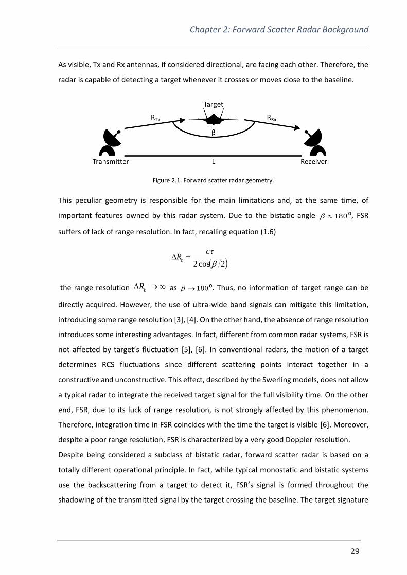
Forward Scatter Radar Geometry
FSR is a specific case of bistatic radar having the bistatic angle 180 ⁰. This implies the
bistatic range is LRR RxTx , with TxR , RxR and L the distances transmitter-target, target-
receiver and the baseline, respectively. Figure 2.1 shows the forward scatter radar geometry.
Chapter 2: Forward Scatter Radar Background
29
As visible, Tx and Rx antennas, if considered directional, are facing each other. Therefore, the
radar is capable of detecting a target whenever it crosses or moves close to the baseline.
Figure 2.1. Forward scatter radar geometry.
This peculiar geometry is responsible for the main limitations and, at the same time, of
important features owned by this radar system. Due to the bistatic angle 180 ⁰, FSR
suffers of lack of range resolution. In fact, recalling equation (1.6)
2cos2
cRb
the range resolution bR as 180 ⁰. Thus, no information of target range can be
directly acquired. However, the use of ultra-wide band signals can mitigate this limitation,
introducing some range resolution [3], [4]. On the other hand, the absence of range resolution
introduces some interesting advantages. In fact, different from common radar systems, FSR is
not affected by target’s fluctuation [5], [6]. In conventional radars, the motion of a target
determines RCS fluctuations since different scattering points interact together in a
constructive and unconstructive. This effect, described by the Swerling models, does not allow
a typical radar to integrate the received target signal for the full visibility time. On the other
end, FSR, due to its luck of range resolution, is not strongly affected by this phenomenon.
Therefore, integration time in FSR coincides with the time the target is visible [6]. Moreover,
despite a poor range resolution, FSR is characterized by a very good Doppler resolution.
Despite being considered a subclass of bistatic radar, forward scatter radar is based on a
totally different operational principle. In fact, while typical monostatic and bistatic systems
use the backscattering from a target to detect it, FSR’s signal is formed throughout the
shadowing of the transmitted signal by the target crossing the baseline. The target signature

Chapter 2: Forward Scatter Radar Background
30
results as a modulation of the direct signal due to the motion of an object nearby Tx and Rx
line of sight. It is then clear that the received signal in FSR is influenced by the presence of a
target crossing and by its motion parameters. Thus, such values can be extracted using specific
processing.
Forward Radar Cross Section
Another way to describe the forward scatter principle is through the Physical Theory of
Diffraction (PTD) [7]. The electromagnetic (EM) field scattered by a target in a bistatic scenario
is composed by the reflected field �⃗� 𝑟𝑒𝑓 and by the shadow field �⃗� 𝑠ℎ [5], [8]. Thus, the total
field can be expressed as follows
shref EEE
( 2.1 )
When the scattering object’s dimension is comparable to or bigger than the wavelength, the
shadow field is concentrated in the forward scattering (FS) region.
Figure 2.2. Scattering mechanism and shadow field forming.
This can be better understood looking at Figure 2.2, which shows the scattering mechanism
at the base of FSR. Due to the presence of a target, the incident field �⃗� 𝑖𝑛𝑐 is back scattered in
different direction and, at the same time, blocked in the FS one, forming the shadow region.
In this area, defined by the target’s contour, the field is equal to zero, 0 shref EEE
[5].
Thus, the target can be seen as a black body, whose shape and coating can be neglected. In
fact, it is only its silhouette to influence the field.
Through the EM mechanism, it is then possible to quantify, in terms of RCS, the way the target
affects the radar system. Formula (1.20), here presented again to simplify the reading,
Chapter 2: Forward Scatter Radar Background
31
2
2
2lim4
Tg
Rx
R E
ER
is the classic definition of the radar cross section. RCS trend defines three different regions,
characterized by the ratio between the target’s physical dimension D and the wavelength
: the Rayleigh region, when D ; the Mie or resonance region, when D ; the optical
region, with D [9]. Generally, for the majority of radars, can be assumed smaller than
the target dimension.
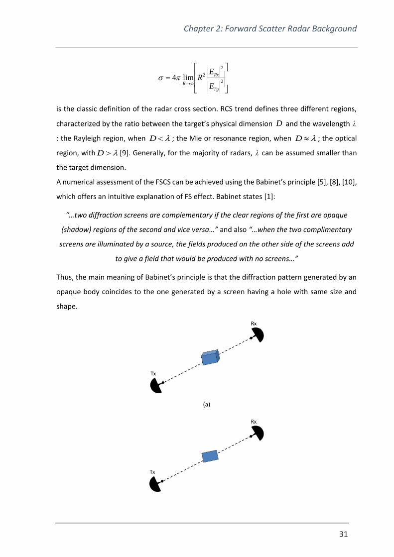
A numerical assessment of the FSCS can be achieved using the Babinet’s principle [5], [8], [10],
which offers an intuitive explanation of FS effect. Babinet states [1]:
“…two diffraction screens are complementary if the clear regions of the first are opaque
(shadow) regions of the second and vice versa…” and also “…when the two complimentary
screens are illuminated by a source, the fields produced on the other side of the screens add
to give a field that would be produced with no screens…”
Thus, the main meaning of Babinet’s principle is that the diffraction pattern generated by an
opaque body coincides to the one generated by a screen having a hole with same size and
shape.
(a)

Chapter 2: Forward Scatter Radar Background
32
(b)
(c)
Figure 2.3. Forward scattering mechanism. A complex 3D target (a) can be replaced with an equivalent 2D shadow (b) which, for the Babinet’s principle, is equivalent to an aperture of same size and shape in an
infinite surface.
The mechanism at the base of forward scatter radar can be summarized through Figure 2.3,
where a complex 3D target, Figure 2.3 (a), is progressively replaced by a 2D shadow silhouette,
Figure 2.3 (b), and finally by an infinite plane having a hole of same size and shape of the
opaque body, Figure 2.3 (c). Therefore, in a forward scatter configuration and operating in
optical region, the FSCR of a target having a silhouette area A can be calculated as following
[2], [11], [12]
2
24
AFS
( 2.2 )
( 2.2 ) shows the FSCR increases as a power of two of the carrier frequency, remembering
221 cfT , and as a power of four of the object linear dimension D , considering 2DA
. Whereas the backscattering RCS, despite increasing with the size of the target, does not
dependent on the transmitted frequency [13], [14].
As intuitive, considering a flat plate as a target, the backscattered signal is equal to the forward
scatter one. For a complex shaped object, instead, the FSCS is greater than the monostatic/
bistatic [13], [14]. This drastic increase in FS cross section, called forward scatter effect [5],
makes possible to improve the power budget problem simplifying the detection of small
targets, the detection of targets at very distant ranges and giving the possibility to transmit
less power, if required. On the top of this, as a direct consequence of the Babinet’s principle,
FSCR does not depend on target material [15], [16]. In fact, it has been demonstrated how the

Chapter 2: Forward Scatter Radar Background
33
magnitudes of two identical objects, one metallic and one covered by absorbing material,
coincide in the forward scatter region and show differences in the region characterized by
bistatic reflection [15], [16]. This feature made FSR an extremely efficient counter-stealth
radar system.
However, it is fundamental to clarify the value of FS expressed in ( 2.2 ) referrers to the only
case in which 180 ⁰. For bistatic angles different from that, the RCS decreases. Thus, it is
important to focus on the FSCS main lobe (ML) FSML . This parameter can be estimated with
the following formula
ffe
FCMLD
( 2.3 )
where ffeD is the maximal target effective dimension [17], [18].
( 2.2 ) and ( 2.3 ) allow to determine some relationships between FSCS and FSCS ML. In fact,
with the increase of the target dimension the radar cross section increases but the main lobe
reduces, narrowing the forward scatter region. The same happens when the transmitted
frequency increases. For a simple target having the effective aperture A defined by ffeD , in
order to clarify the relation between cross section and main lobe in the forward scatter
scenario, it is possible to combine equations ( 2.2 ) and( 2.3 ) as following
24
FSML
Max
FS
A
( 2.4 )
The forward scatter cross section plays an important role in the radar power budget whereas
the main lobe determines the radar coverage area. Therefore, it would be desirable to
increase the value of both these parameters, in the attempt of creating a radar system with
great power benefits and coverage. However, ( 2.4 ) shows the impossibility of doing this.
Quantified the -3dB width of the FS main lobe, the target visibility time, VT , can also be
estimated. This corresponds to the time needed by a target, moving with velocity component
Tgv and crossing at a distance RxR from the receiver, to cross the entire main lobe. VT can be
expressed with the following relation

Chapter 2: Forward Scatter Radar Background
34
Tgffe
Rx
Tg
RxFSMLv
vD
R
v
RT
( 2.5 )
Due to the lack of resolution, FSR target signal does not fluctuate much. As a consequence,
the maximum coherent analysis time for such kind of radar may coincide with the visibility
time. Therefore, remembering that the Doppler frequency resolution Vd Tf 1 , the absence
of range resolution is in part balanced by a good frequency resolution.
What so far described refers to RCS values in the case of 180 ⁰. However , an important
gain in the radar cross section is still present in the antenna sidelobes, enabling a wider
detection area [5].
Figure 2.4 shows the radiation patter of a sphere. Low values of RCS are presented in blue,
high ones in red. The sphere radiates uniformly along almost all the directions. However, as
previously explained, a substantial increase of the RCS is visible in the forward direction.
Therefore, detection of such a target is easier working with a FSR system.
Figure 2.4. Radar cross section of a sphere
This is true whenever operating with target whose dimension is greater than the wavelength,
in the Mie or optical region. As presented in [18] and reported here in Figure 2.5, a clear
evidence of this phenomenon is shown. The normalised RCS values in monostatic and forward
scatter geometry are presented and compared. It is possible to see how when operating in
the Rayleigh region monostatic and FS RCS follow a similar trend, with actually the second one
having a slightly smaller value than the first one. As soon as entering the Mie region, so when
the dimension of the sphere is comparable to the wavelength, the target reflectivity starts to
grow in the FS scenario. The difference between FS and monostatic cross section increases
drastically with the increase of D .
Incident field FS direction

Chapter 2: Forward Scatter Radar Background
35
Moreover, the forward scatter mainlobe width with respect to the diameter of the sphere is
shown in Figure 2.5. The trend verifies what stated by ( 2.3 ): the bigger the dimension of the
target the narrower the FS mainlobe. It is interesting to underline the opposite behaviours of
cross section and mainlobe in FSR.
Numerical valuation of a complex target’s RCS is quite difficult and could be therefore
calculated using software for full wave analysis, like CST Microwave Studio [19]. Results of
simulations calculated for some targets of interest are presented in Table 2.1 [18]. RCS values
at different frequencies are included for bistatic ( 90 ⁰) and forward scatter ( 180 ⁰)
cases.
Table 2.1. Bistatic and forward scatter RCS for different targets. RCS measured in dBsm [18].
λ=3.0 m / f=100 MHz λ=0.3 m / f=1 GHz
BR (β=90⁰) FSR (β=180⁰) BR (β=90⁰) FSR (β=180⁰)
Human
(L=0.5, H=1.8) 6.2 7.6 11.6 22.0
Car
(L=4.8, H=2.2) 9.7 22.5 5.4 41
Figure 2.5. Comparison between normalized monostatic (RCS) and forward scatter (FSCS) cross section and forward scatter mainlobe (θFS) of a sphere of diameter D [18].

Chapter 2: Forward Scatter Radar Background
36
Inflatable boat
(L=2.3, H=1)) 0.6 2.7 -6.6 21.4
Missile
(L=3.6, H=0.5) 2.9 8.9 -6.1 29
Table 2.1 confirms the trend in Figure 2.5. In fact, focusing on the human target, its bistatic
cross section (BCS) and FSCS are close when 6.0D ( 3 m) and get different, with the
FSCS nearly doubling the BCS, for 6D ( 3.0 m).
Figure 2.6. Plane wave incident on a rectangular aperture.
A simplified way to calculate the RCS of a complex target is to describe its silhouette as a
rectangle, as in Figure 2.6, or a composition of them [20]. In fact, the formula modelling the
RCS of a rectangular target is well known in literature [16], [20] and is given by the following
equation
22
2
sin
sinsin
sin
sinsin
4,
eff
eff
eff
eff
ff
FS h
h
l
l
Ae ( 2.6 )
( 2.6 ) shows the RCS of a rectangular plate as function of azimuth, , and elevation, , angles.
It also depends on ffeA ,
ffel and ffeh that are the effective aperture, length and height of the
target, respectively.

Chapter 2: Forward Scatter Radar Background
37
Power Budget in FSR
Power budget is used to predict the performance of a radar system and show the parameters
influencing the received signal. In order to calculate the power budget of a forward scatter
system, two different models can be used: the free space and the two ray path (TRP) one. The
former typically relates to scenarios where the height of the antennas is comparable to the
length of the baseline or the radar’s antennas have a quite narrow illumination beam. In this
case, we talk about free space propagation because the contribution scattered by the surface
can be omitted. On the other hand, the TRP model takes into account the signals reflected by
the surface, since they have the same order of magnitude as those not reflected. Therefore,
the total field depends on the combination of both reflected and not reflected rays.
2.2.3.1 Free Space Model
Forward scatter signal can be described as a composition of two main signals [16], [21]:
• the leakage signal, which is the one transmitted by the Tx in a scenario with no target
around;
• the target signal, which is the one due to the presence of a target crossing the baseline.
The target signal, which carries all the target information, modulates the much stronger
leakage signal. In order to guarantee the operational principle of FSR both signals are
fundamental.
(a)

Chapter 2: Forward Scatter Radar Background
38
(b)
Figure 2.7. Leakage (a) and target (b) signal topologies in free space propagation model.
Figure 2.7 shows the FSR topology for leakage (a) and target signal (b). 1R , 3R and 5R are
direct, transmitter to target and target to receiver signals, respectively. Txh and Rxh are the
heights of transmitter and receiver antennas.
The leakage signal power F
LSP can be calculated using the following formula [22], [23]
FSRxTxTxRxTxTx
F
LS LGGPL
GGPP
2
4
( 2.7 )
where TxP , TxG and RxG are the transmitted power and the transmitter and receiver antenna
gains respectively. 214 RLFS is the free space propagation loss. An extra factor could be
included in ( 2.7 ) in order to take into account the system and environmental losses.
Similarly, the target signal power 𝑃𝑇𝑆𝐹 can be estimated as
TS
RxTx
FSRxTxTxF
TS LRR
GGPP
223
2
4
( 2.8 )
As in ( 2.7 ), in ( 2.8 ) only the free space propagation loss LTS is taken into account. When
2LRR RxTx , so when the target crosses the baseline exactly in the middle, F
TSP reaches its
minimum value. Therefore, as done in Chapter 1 for the monostatic and bistatic case, it is
possible to calculate the FSR range equation as

Chapter 2: Forward Scatter Radar Background
39
4
min
3
2
max4
2S
LGGPL TSFSRxTxTx
( 2.9 )
With minS the minimum value of detectable power level required to achieve the desired
performance.
2.2.3.2 Two Ray Path Model
Differently from the free space propagation model, the two ray path approach takes into
account not only the direct rays but also the reflected ones from the surface. The model,
initially used for wireless communication studies [24], well performs in radar applications [21],
[25].
(a)
(b)
Figure 2.8. Two ray path model. Leakage (a) and target (b) signal.
The topology of both leakage and target signals is presented in Figure 2.8. As shown, the
leakage signal is now the composition of two rays: the direct one, 1R , and the reflected from
the ground 2R . Assuming the transmitter radiates unit power and the use of isotropic
antennas, so that 1RxTxTx GGP , the total leakage signal can be expressed as

Chapter 2: Forward Scatter Radar Background
40
21
21
jj
LS eUeUu ( 2.10 )
where:
• ii RU 4 is the magnitude of the of direct, for 1i and reflected, for 2i , waves;
• ii R2 is the absolute phase of the ray;
• iR is the length of the path;
• is the complex ground reflection coefficient, which depends on ground features,
grazing angle, wavelength and polarization of the antenna.
Depending on the polarization, can be calculate as follows [21], [23]
2
2
2
2
cossin
cossin
cossin
cossin
g
g
H
gg
gg
V
( 2.11 )
( 2.11 ) presents the ground reflection coefficient for vertical (V) and horizontal (H)
polarization of the wave. Lhh RxTx arctan is the grazing angle. 02 fjrg is
the relative dielectric permittivity of the ground and depends on the type of surface,
expressed in terms of relative dielectric constant r and conductivity [23], and on the
frequency. 0 is the dielectric constant, equal to 121085.8 F/m. Typical values of r and
for different surfaces are presented in Table 2.2 [23].
Table 2.2. Ground features. Conductivity and dielectric constant [23].
Surface r
Dry ground 3101 4-7
Average ground 3105 15
Wet ground 2102 25-30
Sea water 0105 81
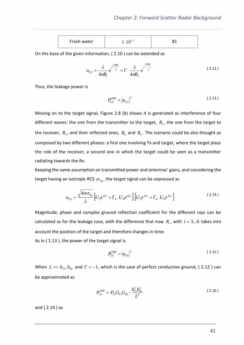
Chapter 2: Forward Scatter Radar Background
41
Fresh water 2101 81
On the base of the given information, ( 2.10 ) can be extended as
21
2
2
2
1 44
Rj
Rj
LS eR
eR
u ( 2.12 )
Thus, the leakage power is
2
SL
TRP
LS uP ( 2.13 )
Moving on to the target signal, Figure 2.8 (b) shows it is generated as interference of four
different waves: the one from the transmitter to the target, 3R , the one from the target to
the receiver, 5R , and their reflected ones, 4R and 6R . The scenario could be also thought as
composed by two different phases: a first one involving Tx and target, where the target plays
the role of the receiver; a second one in which the target could be seen as a transmitter
radiating towards the Rx.
Keeping the same assumption on transmitted power and antennas’ gains, and considering the
target having an isotropic RCS Tg , the target signal can be expressed as
6543
665443
4
jjjjTg
TS eUeUeUeUu ( 2.14 )
Magnitude, phase and complex ground reflection coefficient for the different rays can be
calculated as for the leakage case, with the difference that now iR , with 6...3i takes into
account the position of the target and therefore changes in time.
As in ( 2.13 ), the power of the target signal is
2
TS
TRP
TS uP ( 2.15 )
When RxTx hhL , and 1 , which is the case of perfect conductive ground, ( 2.12 ) can
be approximated as
4
22
L
hhGGPP RxTx
RxTxTx
TRP
LS ( 2.16 )
and ( 2.14 ) as

Chapter 2: Forward Scatter Radar Background
42
4
22
4
22
2
4
RxTg
RxTg
TgTx
TgTxTg
RxTxTx
TRP
TSd
hh
d
hhGGPP
( 2.17 )
with TgTxd
and RxTgd
the projections of the distances transmitter-target and target-receiver
on the ground surface.
( 2.16 ) shows that in specific conditions the two ray path leakage signal can be seen as
function of only height of antennas and baseline. ( 2.17 ) shows still dependence on the
wavelength due to the presence of the target.
(a)
(b)
Figure 2.9. FSR power budget. Leakage signal (a) and target signal (b).
Figure 2.9 presents leakage (a) and target (b) signals’ power budget calculated using the TRP
model, equations ( 2.13 ) and ( 2.15 ), its simplified version, equation ( 2.16 ) and ( 2.17 ), and
10-1
100
101
102
103
-120
-100
-80
-60
-40
-20
0
20
40
60
Baseline(m)
dB
Leakage signal
TRP
TRP simplified formula
Free space propagation
10-1
100
101
102
103
-200
-150
-100
-50
0
50
100
150
Baseline(m)
dB
Target signal
TRP
TRP simplified formula
Free space propagation

Chapter 2: Forward Scatter Radar Background
43
free space propagation model, ( 2.7 ) and ( 2.8 ). Transmitter power, antenna gains and target
RCS have been assumed to be equal to 1 whereas the antenna’s heights equal to 2 m.
Comparing the different approaches, the full and simplified TRP equations provide, as
expected, different results for small values of baselines; on the other hand, for long baselines,
their difference decreases. In fact, as stated before, ( 2.16 ) and ( 2.17 ) guarantee a good
approximation of the power problem when the relation RxTx hhL , is verified. Focussing on
the free space propagation model, it matches, especially for not too big values of baseline,
with the TRP model in case of absence of target. The difference between the two approaches
increases when a target is considered.
Forward Scatter Radar Target Signature
As previously stated, the principle FSR is based on is the shadowing of the signal emitted by
the transmitter due to the presence of a target crossing the Tx-Rx line of sight. Therefore, the
object moving nearby the baseline introduces an amplitude modulation of the leakage signal.
In order to proceed with an analytical calculation of the target signature in FSR, the target is
assumed to follow a linear trajectory and move with a constant speed. For the majority of the
applications and configurations this assumption can be considered realistic.
To better understand how the FSR signature can be modelled, the following analysis focuses
initially on a point-like target. The information of radar cross section is omitted to concentrate
on the phase signature of the moving point [16]. Later, the described trend will be combined
with the information of target RCS. Considering at the receiver a combination of leakage signal
tSLS and target signal tSTS with amplitude LSA and TSA , respectively, the received signal
is
tStStS TSLSRI ( 2.18 )
Taking into account the shadow is characterized by a 2 phase shift with respect to the
direct signal [15], ( 2.18 ) can be written as
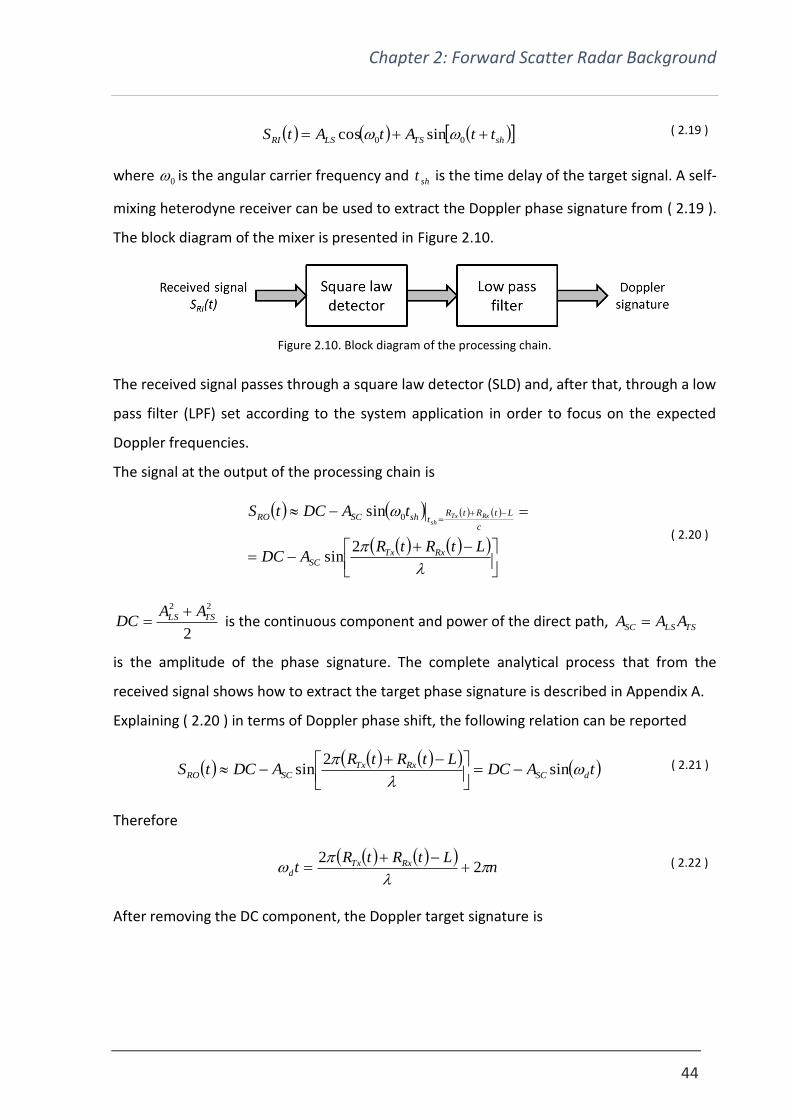
Chapter 2: Forward Scatter Radar Background
44
shTSLSRI ttAtAtS 00 sincos ( 2.19 )
where 0 is the angular carrier frequency and sht is the time delay of the target signal. A self-
mixing heterodyne receiver can be used to extract the Doppler phase signature from ( 2.19 ).
The block diagram of the mixer is presented in Figure 2.10.
Figure 2.10. Block diagram of the processing chain.
The received signal passes through a square law detector (SLD) and, after that, through a low
pass filter (LPF) set according to the system application in order to focus on the expected
Doppler frequencies.
The signal at the output of the processing chain is
LtRtRADC
tADCtS
RxTxSC
c
LtRtRtshSCRO RxTxsh
2sin
sin 0
( 2.20 )
2
22
TSLS AADC
is the continuous component and power of the direct path, TSLSSC AAA
is the amplitude of the phase signature. The complete analytical process that from the
received signal shows how to extract the target phase signature is described in Appendix A.
Explaining ( 2.20 ) in terms of Doppler phase shift, the following relation can be reported
tADCLtRtR
ADCtS dSCRxTx
SCRO
sin
2sin
( 2.21 )
Therefore
n
LtRtRt RxTx
d
2
2
( 2.22 )
After removing the DC component, the Doppler target signature is

Chapter 2: Forward Scatter Radar Background
45
LtRtRAtS RxTx
SCr
2sin ( 2.23 )
Figure 2.11. Point like target Doppler signature and its relationship with the target crossing the baseline.
Figure 2.11 shows the Doppler signature for a point-like target, consisting in a double-sided
chirp signal. The crossing of the isorange ellipsoids by the target determines the change of
phase in the Doppler signature, as visible in figure. 0t is the exact time the point-like target
is on the baseline, since the time origin has been set coinciding with the crossing time. Positive
and negative times refer to the situation in which the target is getting closer and then further
to the baseline, respectively.
Focussing on ( 2.23 ), and remembering TSLSSC AAA , it is evident how the amplitude of the
phase signature depends on the target. In fact, omitted the term related to the leakage signal,
it is tATS to modulate the signature. This term is the target radar cross section and it changes

Chapter 2: Forward Scatter Radar Background
46
in time according to the target position. The calculation of the RCS of complex targets is quite
difficult, approximated models, EM simulations or approximation of target with simple
geometrical surfaces can be used to achieve an accurate estimation.
Figure 2.12. Normalized target Doppler signature without (black) and with (red) RCS.
Figure 2.12 shows a point-like target Doppler signature, in black, and its version modelled with
the RCS of a squared plate, in red. As visible, the amplitude of the signature considering the
RCS clearly shows the effects of the main forward scatter lobe and of the other sidelobes.
Clutter in Forward Scatter Radar
Clutter refers to the return of unwanted radar echoes interfering with the desired echoes
caused by the presence of objects of interest. The need to describe accurately radar clutter
determined investigation, development of models and several measurements of clutter in its
different forms. The problem is extremely challenging because of clutter variability and
because its effect can change drastically from site to site and from geometry to geometry [26].
Environmental non-stationary clutter limits Doppler radar performance significantly. In
monostatic radars, since the ability to discriminate in range and the usual use of directional
antennas, clutter is collected from a restricted area of illumination. Differently, FSR lacks in
range resolution and picks up clutter from a wider area illuminated by its nodes [27]. The main
problems introduced by the presence of clutter lead to:
• decrease of target detection, due to clutter shadowing the target itself;
-15 -10 -5 0 5 10 15-1
-0.5
0
0.5
1
Time, s
Do
pp
ler
sig
na
ture
No RCS
With RCS

Chapter 2: Forward Scatter Radar Background
47
• increase of false alarms.
FSR clutter depends strictly on the main radar applications. In fact, based on the scenario,
vegetation or dynamic sea surface can limit radar performance. Therefore, it has been
necessary to investigate clutter statistics and spectrum for ground based, maritime and
airborne target detection. The last scenario, due to the nature of the application itself, is the
least affected by unwanted echoes.
2.2.5.1 Vegetation Clutter
Wind-blown vegetation has a high impact on ground radar performance due to the
introduction of signal attenuation, scattering and multipath interference. One of the main
challenges of clutter investigation is its dependence on the wind, an extremely unpredictable
parameter.
Measurements at UHF and VHF bands taking into account sites characterized by different
terrain features, from flat open ground to uneven wooded areas, have been proposed [27]–
[29].
(a)

Chapter 2: Forward Scatter Radar Background
48
(b) (c)
Figure 2.13. FSR vegetation clutter. PSDs at different frequencies (a) and PDF at 64 MHz (b) and 173 MHz (c) [27].
Figure 2.13 presents some experimental results concerning FSR vegetation clutter available in
literature [27]. Clutter statistics in terms of power spectral density (PSD) are shown in Figure
2.13 (a). As visible, clutter spectrum width, considering the 10 dB drop, is below 1/2 Hz.
Moreover, the PSD decreases at approximately a rate of 40 dB per decade of Doppler
frequency and the clutter power increases with frequency and wind speed [30]. Furthermore,
according to the measured data the clutter probability density function (PDF) in condition of
medium wind fit well a Weibull distribution. Wind strength and frequency influence the
Weibull distribution shape factor. More precisely, an increase of wind or frequency would
correspond to a decrease of shape factor, as evident comparing Figure 2.13 (b) and (c).
Finally, in order to validate the acquired results a simple method considering a sum of swinging
scattering points moving in a pendulum-like way was used [27]. This approach was intended
to simulate the clutter return from a tree having its branches oscillating due to the wind. Such
simulated model matched the measured date quite accurately.
2.2.5.2 Sea Clutter
As well as vegetation, clutter generated by sea surface can deteriorate radar performance. In
fact, sea waves could act like obstacles and determine backscatter, bistatic or forward scatter
interference, as presented in Figure 2.14.

Chapter 2: Forward Scatter Radar Background
49
Figure 2.14. FSR system in high sea state scenario.
Several studies focused on the investigation of radar scattering from sea surface in order to
clarify the problem [31]–[36]. As consequence of that, it has been able to extract and analyse
both sea clutter spectral and statistical features for different operating frequencies, sea states
and locations.
(a)
(b) (c)
Figure 2.15. FSR sea clutter measurements. Normalized PSDs in different scenarios (a), PDFs (b) and CDFs (c) of normalized sea clutter at 7.36 and 24 GHz [37].

Chapter 2: Forward Scatter Radar Background
50
Figure 2.15 shows results from sea clutter measurements undertaken during a PhD project
focused on the analysis of maritime FSR clutter [37]. Normalized PSDs of various
measurements are proposed in Figure 2.15 (a). Different frequencies and baselines were used.
The results show the independence of FSR sea clutter spectrum on operational frequency and
baseline, at least in the used ranges. The independence on the baseline is related to the fact
that the major clutter contribute comes from the areas around Tx and Rx, as proved in [38].
Moreover, the spectra, considering a 10 dB drop, are limited within the 1 Hz Doppler
frequency. In addition to that, the PSD decreases at approximately a rate of 25-40 dB per
decade of Doppler frequency. Focussing on Figure 2.15 (b) and (c) it is visible how the clutter
statistics well fits a Rayleigh distribution. As for the spectrum, according to the experimental
results, the shape of distribution of sea clutter does not depend on carrier frequency, sea state
level and FSR geometry.
2.3 Radars on Moving Platforms
Part of this work focuses on the investigation of forward scatter radar having transmitter and
receiver installed on a moving platform. Therefore, it is worth looking at some basic
information related to this kind of radar configuration. Moving radars are widely used,
installed on both ground, maritime or airborne platforms. Their application range is extremely
vast and, depending on their purpose, wanted and unwanted echoes change. For example, for
some uses return from ground is considered clutter, for others it is the wanted signal instead.
The following pages briefly summarize which are the main issue of such kind of systems,
entirely caused by the motion of the radar which determine the presence of Doppler shift and
clutter Doppler spread.
Ground Return Spectrum
Clutter is one of the major problems of radar, especially if installed on a moving platform. In
fact, interference introduced by unwanted targets is always present. Therefore, it is
fundamental to separate these unwanted contributes from the desired ones. One of the most
challenging issues for moving radars is the Doppler effect introduced by their motion. Since
this could deteriorate the performance of the radar, its estimation is required in order to

Chapter 2: Forward Scatter Radar Background
51
mitigate the problem. A better understanding of the effects introduced by the ground is
fundamental to understand what would happen in presence of a target. The problem could
be divided in two cases:
• scenario in which radar and target move in opposite direction;
• scenario in which radar and target move in the same direction.
Figure 2.16. Opposite direction movement. The Doppler frequency of the target is bigger than the one of the ground.
The first case, presented in Figure 2.16, can be considered as a favourable one. rv and
tgv are
radar and target velocity, respectively. Moreover, Figure 2.16 shows, at the bottom, the
Doppler frequency contributes related to clutter and target. The interference introduced by
unwanted returns depends on the radar’s speed whereas the Doppler effect associated to the
target depends on how radar and target’s speeds combine together. Since radar and target
move in opposite direction, their relative velocity is greater than the radar’s one. Therefore,
the target Doppler frequency is bigger than the clutter’s one. In this situation, the target would
be detected without problems.
Differently, the second scenario refers to a situation in which radar and target move in the
same direction.

Chapter 2: Forward Scatter Radar Background
52
(a)
(b)
(c)
(d)
Figure 2.17. Same direction movement. The Doppler frequency of the target is lower than the one of the ground.
The scenario is visually presented in Figure 2.17 (a). Since radar and target share the same
direction their relative speed will be smaller than the contribution from the ground. Therefore,
the target contribute will shift to the left. According to which is the relative speed, the target
shift could be within the ground contribute or more negative than it. In the first case, the
target falls in the clutter contribute and, depending on if its return is higher or lower than the
clutter one, it could be detected, Figure 2.17 (c), or not, Figure 2.17 (b). When the speed of

Chapter 2: Forward Scatter Radar Background
53
the target is much greater than the radar one, instead, the target Doppler shift could also
appear visible on the negative frequency half of the spectrum Figure 2.17 (c) [39].
2.4 Moving Ends Forward Scatter Radar
Moving ends forward scatter radar is an FSR configuration having transmitting and receiving
nodes installed on moving platforms which are free to arbitrarily move. Therefore, a
conventional FSR, characterized by non-moving Tx and Rx, can be considered a special case of
moving end FSR.
Advantages and disadvantages of this configuration have been already listed in Chapter 1. This
section aims to explain the differences with respect to a stationary FSR and the difficulties this
system should face.
Figure 2.18. Moving forward scatter radar scenario.
Figure 2.18 shows a possible FSR scenario where both transmitter and receiver are installed
on ships and moving on the sea surface. As intuitive, in order to guarantee the operation in
forward scatter mode the transmitter and receiver antennas should point at each other. In an
ordinary situation, this can be achieved with omnidirectional antennas. The motion of the two
FSR nodes allows to monitor a broader area whereas a typical FSR guarantees only perimetral
surveillance.
The operational principles are the same for both stationary and moving FSR. However, the
motion of Tx and Rx nodes determines some differences which need to be considered when

Chapter 2: Forward Scatter Radar Background
54
investigating this radar system. Despite that this configuration differs from a usual FSR only
for the fact that now transmitter and receiver can move, this introduces a vast scenario of
unpredictability. In fact, there are not limitations to the movements of the system nodes, and
therefore a limitless combination of geometries could be thought.
Due to the varying position of the FSR nodes, the length of the baseline changes over time.
This is an important aspect to take into account when modelling the system because it will
influence several FSR aspects, such as power budget and RCS.
A variation of the baseline results in a variation of leakage and target signal, as understandable
from ( 2.7 ) and ( 2.8 ) in case of free space approximation, or from ( 2.10 ) and ( 2.14 ), if
considering the TRP model. This change in the power level could determine an operational
limit, impeding target detection.
The modelled signal in ( 2.23 ) shows also its strong dependence on the baseline. In case of
moving transmitter/ moving receiver FSR the equation changes as following
tLtRtRAtS RxTx
SCr
2sin ( 2.24 )
( 2.24 ) shows how not only the distances transmitter-target and target-receiver but also the
baseline L is now function of the time.
Moreover, the motion of the radar nodes changes the way the target is seen while crossing.
In fact, its viewing angle varies in time. This is conceptually an advantage because it could
allow reconstructing different profiles of the target and eventually improving its identification.
However, from the modelling and processing point of view, its radar cross section will change
in time, making the attempt to calculate the RCS mode more complex. Thus, for simple shapes
calculation of the cross section can still be determined taking into account the motion of Tx
and Rx.
Another problem this configuration could be afflicted from is the extremely remote case in
which the target is moving in such way to always remain on the baseline. This is obviously an
extreme scenario and clearly very rare. However, if considering for example the case of
receiver moving, as in [41], when the target speed to Rx speed ratio is equal to target-Tx range

Chapter 2: Forward Scatter Radar Background
55
to Rx-Tx range ratio ( LRvv TxRxTg ) the target would stay always on the baseline preventing
any possible detection [41].
As discussed in Section 2.3, one of the main issues for radar installed on moving platforms is
the unwanted return from clutter. Therefore, also this proposed FSR evolution is affected by
clutter problem. Return from surrounding areas could deteriorate the system capability of
detection. Doppler shift and clutter Doppler spread are expected.
2.5 Summary
This chapter presents all the theoretical background necessary to the reader to understand
the work contained in the following part of the thesis. A full explanation of the forward scatter
radar theory has been proposed in the first part of the chapter. FSR geometry, its advantages
and limitations, the forward scatter principle and the target radar cross section have been
described. After that, a description of the power budget problem has been reported, using
both free space and two ray path propagation models. Moreover, returns from target and
clutter in FSR have been discussed.
After the main section focused on FSR, the second part of the chapter has been dedicated to
radars installed on moving platforms. The focus has been oriented on their applications and
especially the main issue generated by the motion of the radar.
To conclude, the first two sections of the chapter have been mixed together to introduce one
innovative configuration investigated in this thesis project, a forward scatter radar system
with transmitter and receiver installed on moving platforms. In this last section, the
differences between a typical FSR and the new one proposed have been presented to the
reader. The fact that Tx and Rx are free to move changes the system and introduces some new
challenges. In fact, the power budget varies and the processing has to take into account Tx
and Rx motion. Moreover, the system is affected by Doppler shift and clutter Doppler spread
which could decrease the radar operational abilities.

Chapter 2: Forward Scatter Radar Background
56
2.6 Bibliography
[1] N. J. Willis, Bistatic radar. Edison, NJ: SciTech Publishing, 2005.
[2] N. J. Willis and H. Griffiths, Eds., Advances in bistatic radar. Raleigh, NC: SciTech Pub,
2007.
[3] M. Cherniakov, M. Gashinova, C. Hu, M. Antoniou, V. Sizov, and L. Y. Daniel, ‘Ultra
wideband forward scattering radar: Concept and prospective’, in 2007 IET International
Conference on Radar Systems, 2007, pp. 1–5.
[4] L. Y. Daniel, E. G. Hoare, M. Gashinova, A. Svintsov, M. Cherniakov, and V. Sizov, ‘Ultra-
wideband forward scatter radar fence for maritime surveillance #x2014; Initial
experimental results’, in 2010 IEEE Radar Conference, 2010, pp. 526–531.
[5] M. Cherniakov and D. V. Nezlin, Bistatic radar: principles and practice. Southern Gate
(Chichester): John Wiley & Sons, 2007.
[6] M. Cherniakov, R. S. A. R. Abdullah, P. Jancovic, M. Salous, and V. Chapursky,
‘Automatic ground target classification using forward scattering radar’, Sonar and
Navigation IEE Proceedings - Radar, vol. 153, no. 5, pp. 427–437, Oct. 2006.
[7] P. I. Ufimt︠ s︡ev, Fundamentals of the physical theory of diffraction. 2014.
[8] V. S. Chernyak, Fundamentals of multisite radar systems: multistatic radars and
multiradar systems. Amsterdam, The Netherlands: Gordon and Breach Science Publishers,
1998.
[9] M. I. Skolnik, Ed., Radar handbook, 3rd ed. New York: McGraw-Hill, 2008.
[10] M. Born and E. Wolf, Principles of optics: electromagnetic theory of propagation,
interference and diffraction of light, 7th expanded ed. Cambridge ; New York: Cambridge
University Press, 1999.
[11] K. M. Siegel and et al., ‘Bistatic Radar Cross Sections of Surfaces of Revolution’,
Journal of Applied Physics, vol. 26, no. 3, pp. 297–305, Mar. 1955.
[12] K. M. Siegel, ‘Bistatic Radars and Forward Scattering’, in Proceedings of 1958
National Conference on Aerospace and Electronics, Daytonb, Ohio, 1958.
[13] M. I. Skolnik, ‘An Analysis of Bistatic Radar’, IRE Transactions on Aerospace and
Navigational Electronics, vol. ANE-8, no. 1, pp. 19–27, Mar. 1961.
[14] M. Gashinova, L. Daniel, K. Kabakchiev, V. Sizov, E. Hoare, and M. Cherniakov,
‘Phenomenology of signals in FSR for surface targets detection’, in IET International
Conference on Radar Systems (Radar 2012), 2012, pp. 1–6.
[15] R. E. Hiatt, K. M. Siegel, and H. Weil, ‘Forward Scattering by Coated Objects
Illuminated by Short Wavelength Radar’, Proceedings of the IRE, vol. 48, no. 9, pp. 1630–
1635, Sep. 1960.
[16] M. Gashinova, L. Daniel, V. Sizov, E. Hoare, and M. Cherniakov, ‘Phenomenology of
Doppler forward scatter radar for surface targets observation’, Sonar Navigation IET
Radar, vol. 7, no. 4, pp. 422–432, Apr. 2013.

Chapter 2: Forward Scatter Radar Background
57
[17] M. Contu et al., ‘Passive Multifrequency Forward-Scatter Radar Measurements of
Airborne Targets Using Broadcasting Signals’, IEEE Transactions on Aerospace and
Electronic Systems, vol. 53, no. 3, pp. 1067–1087, Jun. 2017.
[18] M. Gashinova et al., ‘Signal characterisation and processing in the forward scatter mode
of bistatic passive coherent location systems’, EURASIP Journal on Advances in Signal
Processing, 2013.
[19] ‘CST Microwave studio’ [Online]. Available: https://www.cst.com/Products/CSTMWS.
.
[20] L. Daniel, M. Gashinova, and M. Cherniakov, ‘Maritime target cross section estimation
for an ultra-wideband forward scatter radar network’, in 2008 European Radar Conference,
2008, pp. 316–319.
[21] V. Sizov, M. Cherniakov, and M. Antoniou, ‘Forward scattering radar power budget
analysis for ground targets’, Sonar Navigation IET Radar, vol. 1, no. 6, pp. 437–446, Dec.
2007.
[22] T. S. Rappaport, Wireless communications: principles and practice, 2nd ed. Upper
Saddle River, N.J: Prentice Hall PTR, 2002.
[23] J. D. Parsons, The mobile radio propagation channel, 2nd ed. Chichester : New York:
J. Wiley, 2000.
[24] D. E. Kerr and Institution of Electrical Engineers, Eds., Propagation of short radio
waves. London, U.K: P. Peregrinus on behalf of the Institution of Electrical Engineers,
1987.
[25] F. E. Nathanson, J. P. Reilly, and M. Cohen, Radar design principles: signal processing
and the environment, Second Edition. Edison, NJ: Scitech Publishing, 1999.
[26] J. B. Billingsley, Low-angle radar land clutter: measurements and empirical models.
Norwich, N.Y. : Stevenage, UK: William Andrew Pub. : SciTech Pub. ; Institution of
Electrical Engineers, 2002.
[27] M. Gashinova, M. Cherniakov, N. A. Zakaria, and V. Sizov, ‘Empirical model of
vegetation clutter in forward scatter radar micro-sensors’, in 2010 IEEE Radar Conference,
2010, pp. 899–904.
[28] V. Sizov, M. Gashinova, N. Zakaria, and M. Cherniakov, ‘VHF communication channel
characterisations over complex wooded propagation paths with applications to ground
wireless sensor networks’, Antennas Propagation IET Microwaves, vol. 7, no. 3, pp. 166–
174, Feb. 2013.
[29] N. N. Ismail, N. E. A. Rashid, Z. I. Khan, N. E. A. Rashid, and M. F. A. Rashid,
‘Measurement, processing and modeling of a tropical foliage clutter using Forward Scatter
Radar micro-sensor network with VHF and UHF bands’, in 2015 International Conference
on Radar, Antenna, Microwave, Electronics and Telecommunications (ICRAMET), 2015,
pp. 76–81.
[30] V. Sizov, C. Hu, M. Antoniou, and M. Cherniakov, ‘Vegetation clutter spectral
properties in VHF/UHF bistatic doppler radar’, in 2008 IEEE Radar Conference, 2008, pp.
1–6.

Chapter 2: Forward Scatter Radar Background
58
[31] V. Fabbro, C. Bourlier, and P. F. Combes, ‘Forward Propagation Modeling Above
Gaussian Rough Surfaces by the Parabolic Shadowing Effect’, Prog. Electromagn. Res.,
vol. 58, pp. 243–269, 2006.
[32] C. Beard, I. Katz, and L. Spetner, ‘Phenomenological vector model of microwave
reflection from the ocean’, IRE Transactions on Antennas and Propagation, vol. 4, no. 2,
pp. 162–167, Apr. 1956.
[33] C. Beard and I. Katz, ‘The dependence of microwave radio signal spectra on ocean
roughness and wave spectra’, IRE Transactions on Antennas and Propagation, vol. 5, no.
2, pp. 183–191, Apr. 1957.
[34] J. R. Smith et al., ‘Electromagnetic forward-scattering measurements over a known,
controlled sea surface at grazing’, IEEE Transactions on Geoscience and Remote Sensing,
vol. 42, no. 6, pp. 1197–1207, Jun. 2004.
[35] D. E. Freund, N. E. Woods, H.-C. Ku, and R. S. Awadallah, ‘Forward Radar propagation
over a rough sea surface: a numerical assessment of the Miller-brown approximation using
a horizontally polarized 3-GHz line source’, IEEE Transactions on Antennas and
Propagation, vol. 54, no. 4, pp. 1292–1304, Apr. 2006.
[36] M. Gashinova, K. Kabakchiev, L. Daniel, E. Hoare, V. Sizov, and M. Cherniakov,
‘Measured forward-scatter sea clutter at near-zero grazing angle: analysis of spectral and
statistical properties’, Sonar Navigation IET Radar, vol. 8, no. 2, pp. 132–141, Feb. 2014.
[37] K. Kabakchiev, ‘Maritime Forward Scatter Radar: Data Collection and Clutter
Analysis’, University of Birmingham, 2014.
[38] M. B. Porfido, A. D. Luca, M. Martorella, M. Gashinova, and M. Cherniakov,
‘Simulation method of Forward Scatter Radar sea clutter based on experimental data’, in
2017 18th International Radar Symposium (IRS), 2017, pp. 1–9.
[39] G. W. Stimson, H. Griffiths, C. Baker, and A. Adamy, Introduction to airborne radar,
Third edition. Edison, NJ: SciTech Publishing, 2014.
[40] T. M. Hyltin, T. D. Fuchser, H. B. Tyson, and W. R. Regueiro, ‘Vehicular Radar
Speedometer’, 1973.
[41] A. De Luca, L. Daniel, K. Kabakchiev, E. Hoare, M. Gashinova, and M. Cherniakov,
‘Maritime FSR with moving receiver for small target detection’, in 2015 16th International
Radar Symposium (IRS), 2015, pp. 834–839.
Chapter 3: Target Signature and Parameter Estimation
59
Target Signature and Parameter
Estimation
Glossary of Abbreviations
FSCS Forward Scatter Cross Section
FSML Forward Scatter Main Lobe
FSR Forward Scatter Radar
LoS Line of Sight
MISL Microwave Integrated System Laboratory
RCS Radar Cross Section
Rx Receiver
SNR Signal to Noise Ratio
Tx Transmitter
3.1 Introduction
This chapter focuses on the effects the presence of a target has on a forward scatter radar
(FSR) system. The aim is to show the reader how the target Doppler signature changes
according to either system or target characteristics. As well as these aspects, possible
techniques to extract information about the motion of the target will be introduced.
The chapter is divided in two main parts:
• First part: focuses on the description of the Doppler signature and the possibility to
extract target’s motion parameters when transmitter (Tx) and receiver (Rx) are not
moving. This section considers two different approaches: the already existing one
operating in time domain and a new developed one operating in frequency domain;

Chapter 3: Target Signature and Parameter Estimation
60
• Second part: concentrates on the moving transmitter/ moving receiver FSR
configuration. Similarly to the previous part, Doppler signature and a developed
method to extract target’s kinematic parameters are discussed.
Target signature’s simulations are presented, showing how parameters such as target’s speed,
crossing angle and crossing point influence the Doppler signature. Moreover, methods to
extract target’s motion parameters are proposed together with their performance on
simulated and real data.
The personal contribution to this chapter is:
• Development of an innovative processing to estimate target’s motion parameters
using the spectrogram of the Doppler signature. Moreover, it has been necessary to
understand how the spectrogram changes according to the motion of the crossing
object. Such investigation has required to undertake a big quantity of measurements
in different environments (ground, maritime and air) using different frequencies,
targets, target’s speeds and trajectories and baselines. The recorded data has been
processed, analysed and compared to achieve a deep understanding of the issue. In
addition to that, the developed processing has been tested in difficult scenarios where
the already existing algorithm was not offering good performance, such as highly
cluttered acquisitions and cases of very small or very big targets crossing;
• Investigation of a moving transmitter/ moving receiver FSR configuration. This has
required the determination of a new way to simulate the target cross section and the
received Doppler signature, considering the motion of Tx and Rx. Moreover, the
already existing processing operating on the phase signature of the moving crossing
object has been modified to allow the extraction of kinematic parameters in the case
of moving ends FSR. As for the previous point, simulations have been compared to real
data. That has required to undertake several measurements. In the specific, I did not
take part in the experimental campaign. However, I have did process all the acquired
data.

Chapter 3: Target Signature and Parameter Estimation
61
3.2 Simulated Target Doppler Signature in Time Domain
A complete description of how to extract the target Doppler signature from the received signal
has been discussed in Chapter 2. This section aims to reveal which parameters influences the
extracted signal and how. In fact, only a full understanding of the way the Doppler signature
changes according to external factors makes possible to identify a method to extract target’s
information.
For the following considerations, let us assume to work with a stationary FSR, remembering
that this can be seen as a particular case of moving ends forward scatter radar.
To understand how the target’s motion influences the phase signature, it is important to have
in mind the forward scatter geometry, shown in Figure 3.1. In the figure, a maritime target
crosses the forward scatter radar baseline, L . TxR and RxR are the distances transmitter-
target and target-receiver, respectively. The target moves with a velocity 𝑣𝑇𝑔⃗⃗ ⃗⃗ ⃗⃗ , assumed
constant during the crossing. Due to the nature of the targets and the length of the visibility
time, this can be considered quite accurate. cpx is the crossing point, the distance between
the crossing and the transmitter. ca is the crossing angle, defined as the angle formed by the
intersection between the target’s trajectory and the baseline.
Figure 3.1. Forward scatter geometry.
The Doppler signature is function of target’s speed, crossing angle and crossing point. In fact,
these three parameters influence the values of TxR and RxR , which can be calculated as

Chapter 3: Target Signature and Parameter Estimation
62
22
22
sincos
sincos
tvytvxxR
tvytvxxR
caTgRxcaTgcpRxRx
caTgTxcaTgcpTxTx
( 3.1 )
where the couples ( Txx , Txy ) and ( Rxx , Rxy ) represent the positions of transmitter and receiver
on the x and y plane.
Influence of Transmitting and Target Parameters on the Doppler Signature
Given the formula of the target phase signature, the Doppler signature is influenced by:
• radar operational frequency;
• target speed;
• target crossing angle;
• target crossing point.
Thus, using (2.27) it is possible to simulate the target signature and visualize the variations
introduced by the alteration of such listed parameters.
Figure 3.2 shows the effects of the transmitted frequency on the received target signature.
The distance transmitter-receiver L is 450 m. In the simulations a rectangular plate (2.8x0.5)
m, length and height of the target respectively, crosses the baseline in the middle, with a
crossing angle 90ca ⁰. Thus, it moves perpendicularly to the Tx-Rx line of sight (LoS).
Target’s speed is 2 m/s.
(a)

Chapter 3: Target Signature and Parameter Estimation
63
(b) (c)
Figure 3.2. Target Doppler signature variations according to the operational frequency: 1 GHz (a), 2 GHz (b) and 4 GHz (c).
The transmitted frequency, which appears in the Doppler signature formula as tfc ,
clearly modifies the received signal, as visible in Figure 3.2. A simulated signature and the
target’s RCS at 1 GHz are proposed in Figure 3.2 (a) to show how the signature is shaped by
the RCS. The forward scatter mainlobe and the first side lobes are clearly visible. The figure
pictures a 30 s interval in which the target approaches the FSR system (approximately from 0
to 10 s), is in the forward scatter region (approximately from 10 to 20 s) and finally moves
away from the radar (approximately from 20 to 30 s). At 15t s the target is exactly on the
baseline. An increase of the operational frequency corresponds to a quicker phase change.
This can be explained thinking about the isorange ellipsoids; in fact, the higher is the frequency
the closer two sequential isorange ellipsoids are. As a result, the target Doppler signature gets
more dense, as visible comparing Figure 3.2 (a), (b) and (c). Moreover, the increase of the
frequency by a factor X narrows the FS mainlobe by the same factor, as shown in ( 2.3 ). This
is confirmed by Figure 3.2, where, moving from (a) to (b) to (c), the transmitted frequency
constantly doubles (1, 2 and 4 GHz respectively) and the mainlobe halves. With the Doppler
signature getting denser, more side lobes start to be visible in the same time slot.
Clarified what happens when the transmitted frequency varies, let us understand which are
the effects of the target’s motion on the Doppler signature. In the following picture, the
simulated scenario is the same as before, a baseline equal to 450 m and target crossing
perpendicularly in the middle of it. The transmitted frequency is set at 2 GHz.

Chapter 3: Target Signature and Parameter Estimation
64
(a) (b)
Figure 3.3. Target Doppler signature variation according to target's speed: 1 m/s (a), and 4 m/s (b).
Figure 3.3 shows simulated results for different target speeds. The crossing object moves with
a speed of 1 m/s in (a) and 4 m/s in (b). For the analysis Figure 3.2 (b), which refers to the
same scenario but with the target’s speed equal to 2 m/s, can be considered as well. The effect
of target’s speed on the phase signature is similar to the one determined by the change of
frequency. As the crossing object moves with higher speed, its signature results more
compressed. Indeed, an increase of the speed determines a decrease for time necessary to
the target to cross the forward scatter region. This is well presented in Figure 3.3 (a) and (b),
together with Figure 3.2 (b) where results show effect similar to the narrowing of the RCS main
lobe.
Keeping all the parameters but the crossing angle fixed allows us to understand the impact of
this variable on the FSR system. For this purpose, a set of simulation in the same scenario has
been repeated. Baseline, crossing point and speed are 450 m, 225m and 2 m/s, respectively.
The transmitted frequency is maintained 2 GHz.

Chapter 3: Target Signature and Parameter Estimation
65
(a) (b)
Figure 3.4. Target Doppler signature variation according to target's crossing angle: 30⁰ (a), and 60⁰ (b).
The effects of the variation of the target’s crossing angle are shown in Figure 3.4. (a) and (b)
refer to simulated scenarios with a target crossing with 30ca ⁰ and 60ca ⁰, respectively.
Like previously, Figure 3.2 (b) can be used again as element of comparison, corresponding to
the case 90ca ⁰. Intuitively, if considering the same crossing point, the time the target
requires to cross the forward scatter area is minimum if the object moves perpendicularly to
the baseline, 90ca , and it increases for 90ca ⁰. This is confirmed by Figure 3.4 (a) and
(b) and Figure 3.2 (b), where, going from situation of 30 degrees crossing to one of 90 degrees,
the target main lobe gets narrower.
The last influencing parameter it is worth to focus on is the crossing point cpx . The simulated
scenario is the same previously described, with 90ca ⁰ and the crossing point changing.
Figure 3.2 (b) and Figure 3.5 (a) and (b) show the target Doppler signature for a crossing in the
middle of the baseline (225 m from Rx), 125 m and 25 m far from the receiver, respectively.
Crossings near the transmitter have not been considered because, in case of Tx and Rx
stationary, they would determine similar effects, due to the symmetry of the system. Results
show how the closer is the crossing to one of the nodes the more compressed is the Doppler
signature.

Chapter 3: Target Signature and Parameter Estimation
66
(a) (b)
Figure 3.5. Target Doppler variation according to target's crossing point: 125 m (a) and 25 m (b) far form Rx.
It is interesting to repeat the analysis on the crossing point considering a target not moving
orthogonal to the baseline. In fact, as proposed in Figure 3.4 (a), Figure 3.6 (a) and Figure 3.6
(b), due to the combination of crossing angle 90ca ⁰ (in the specific 30ca ⁰) and crossing
close to one of the nodes, the Doppler signature is asymmetric. The asymmetry, has shown in
Figure 3.6 (b), is higher when the target crosses closer to either Tx or Rx.
(a) (b)
Figure 3.6. Target Doppler variation according to target's crossing point: 125 m (a) and 25 m (b) far form Rx when the crossing angle is 30⁰.

Chapter 3: Target Signature and Parameter Estimation
67
3.3 Estimation of Target Motion Parameters in Time Domain
The previous section has presented the target Doppler signature and its dependence on target
motion parameters, such as speed, crossing angle and crossing point. Before the beginning of
this PhD project, a specific processing was developed to extract target’s kinematic parameters
from the Doppler signature [1]. This approach is based on the concept that, according to
optimal detection theory [2], maximization of the signal to noise ratio (SNR) can be achieved
through the use of a matched filter [3]. Such filter is characterized by an impulse response
)(th equal to the complex conjugate of the input signal.
Therefore, the maximum SNR can be obtained correlating the received signal with a reference
signature which is the complex conjugated of it, as following
2/
2/
*,
T
T
rrefrefropt tStSdtStSS ( 3.2 )
with T the integration time.
The target Doppler signature being a function of target’s speed, crossing angle, crossing point
and forward scatter cross section (FSCS), all these values should be considered in the
generation of the reference signature. However, the reconstruction of the amplitude
parameter, referring to a specific target FSCS pattern, is particularly complex, since the
characteristics of the object cannot be known in advance. Despite that, it has been shown in
[1] how the correlation between functions quickly alternating their signs is mainly dependent
on their actual sign itself, rather than the variation in amplitude.
Figure 3.7, showing the results presented in [1], aims to clarify the role of different amplitudes
and phases in the correlation between two chirp-like signatures. In (a) three chirps have been
modelled using different envelops: rectangular (rect), FSCS (rect&RCS) and Kaiser window
(rect&wind). Their correlations are reported in Figure 3.7 (b). Analogously, two different chirps
differing in frequency by 10% are shown in (c) with their correlations in (d). Comparing Figure
3.7 (b) and (d), it is visible how a difference in phase influences the resulting correlation more
than a difference in amplitude. Consequently, in the following approach the target RCS is
substituted by a window function, which, as visible in Figure 3.7 (b), introduces a very small
loss.
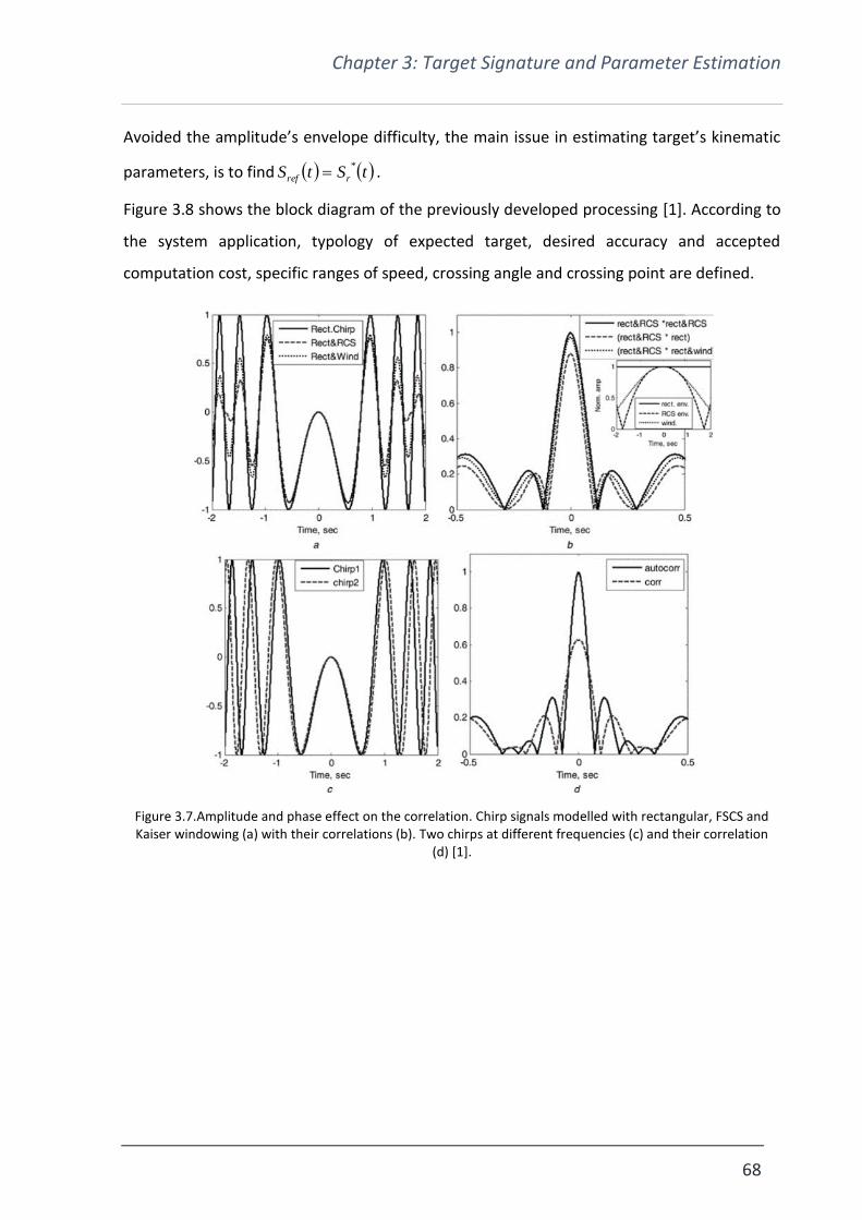
Chapter 3: Target Signature and Parameter Estimation
68
Avoided the amplitude’s envelope difficulty, the main issue in estimating target’s kinematic
parameters, is to find tStS rref
* .
Figure 3.8 shows the block diagram of the previously developed processing [1]. According to
the system application, typology of expected target, desired accuracy and accepted
computation cost, specific ranges of speed, crossing angle and crossing point are defined.
Figure 3.7.Amplitude and phase effect on the correlation. Chirp signals modelled with rectangular, FSCS and Kaiser windowing (a) with their correlations (b). Two chirps at different frequencies (c) and their correlation
(d) [1].

Chapter 3: Target Signature and Parameter Estimation
69
Figure 3.8. Processing block diagram.
Thus, the estimation of the target motion parameters is achieved through the use of a bank
of reference signatures generated using ( 2.27) and shaped through the use of a window.
These reference signatures kjiS ,,
are built considering all the possible combinations of speed
v , crossing angle ca and crossing point cpx values included in the set ranges. i , j and k are
the indices referring to the specific values of these kinematic parameters. These simulated
waveforms are then correlated to the received one. The correlation indicates the level of
similarity between two different waveforms, with the maximum match resulting in the
autocorrelation. Therefore, the reference signature determining the highest value of
correlation among the all calculated, kmjmimS ,,
, is selected as the most similar to the received
signal. Once this waveform is picked, knowing with value of speed, crossing angle and crossing
point generated it, the extraction of target motion parameters imv , jmca _
and kmcpx
_ is
straightforward.
This processing has shown good capabilities in the estimation of the motion of the target. To
provide the reader an example of the results achieved using this technique, Figure 3.10 shows
a comparison between measured and simulated signatures presented in [1].
Figure 3.10 presents results from a maritime experiment where a target crossed the baseline
describing multiple trajectories. The controlled target was a two-seater inflatable boat
acquired by the Microwave Integrated System Laboratory (MISL). Due to the several
measurements undertaken in maritime environment, a maritime controlled target was
needed. Figure 3.9 shows our target during one of the trials. Being such a boat the main target
for all the results described in this chapter, a more detailed description of its characteristics
are given in appendix B. GPS loggers provide information about the boat motion.
Rx Doppler signature
detector SR
Bank of reference
functions Si,j,k
Si,j,k= S(vi,αca_j,cxp_k)
Maximum of
correlation Sim,jm,km
Extraction of
vim, αca_jm, xcp_km

Chapter 3: Target Signature and Parameter Estimation
70
Figure 3.9. MISL boat. It is the main target used during our maritime measurements.
Figure 3.10 shows results from three different scenarios where the controlled target moved
with different trajectories. Experimental geometries, measured Doppler signatures and
simulated ones built using the values of speed, crossing angle and crossing point estimated
with the introduced processing are presented in the figure. Visually, it can be observed a good
match between measured and simulated data. Confirmation of such good performance can
be obtained looking at the comparison between the real kinematic parameters, measured via
GPS loggers, and the estimated ones proposed in Table 3.1.
Table 3.1. Comparison between real and extracted target’s motion parameters.
Scenario (a) Scenario (b) Scenario (c)
GPS Extracted GPS Extracted GPS Extracted
Speed (km/h) 18.5-
19.1 19.08
12.2-
13.0 13
16.7-
19.1 17.64
Crossing angle (⁰) ≈90 90 ≈90 90 ≈60 60
Crossing point from
middle BL (m) 12 20 85.5 80 40 60
As visible in Table 3.1, the described processing well estimates target motion parameters.

Chapter 3: Target Signature and Parameter Estimation
71
Figure 3.10. Google maps scenario with target’s trajectory and comparison between measured and simulated signature for crossing in the middle of the baseline (a), crossing very close to the receiver (b)
and crossing at an angle (c) [1].
3.4 Simulated Target Doppler Signature in Frequency Domain
The time domain approach of looking at the Doppler signature provides good performance in
target detection and parameter estimation. However, the processing described in the
previous section can be time consuming, depending on the desired accuracy, and presents
some limitations whenever the acquired signature does not have the typical chirp-like
structure. Therefore, in this scenario the estimation of target motion parameters could be
Chapter 3: Target Signature and Parameter Estimation
72
affected by high error or even be impossible. Specific difficult cases could arise when the
system is affected by high cluttered environment or when the receiver is shadowed by the
target [4]. For this reason, during the course of this PhD project, one of the main tasks has
been to develop a new method allowing to estimate the motion of crossing objects.
An alternative way to look at the acquired Doppler signature enabling target detection and
extraction of information about the movement of the object is through its spectrogram.
The analysis of Doppler signature’s spectrogram offers the opportunity to achieve a good
estimation of target’s kinematic parameters even in difficult scenarios and can be used for
rough estimation, assisting the time domain processing or substituting it in those difficult
cases previously listed.
As done before for the time domain signal, it is extremely important to understand how the
Doppler signature spectrogram changes according to the way the target crosses the baseline.
For the following analysis ( 2.27 ), re-proposed at the beginning of the chapter, is used to
simulate the waveform in time domain. The spectrogram of such signature is obtained using
the fast Fourier transform (FFT). The time domain signal is divided in small parts (for our
application we used 2 s Hamming windows) which are usually overlapping (in our results we
use a 95% overlap) and for each of them an FFT is calculated. Therefore, each part corresponds
to a vertical section of the spectrogram and represents the magnitude of the frequency in a
specific portion of time.
Influence of Transmitting and Target Parameters on the Doppler Signature’s Spectrogram
This section includes analysis and results published in [4], paper focused on the description of
the Doppler signature in frequency domain and the possibility to extract speed information
via the spectrogram.
Before starting the analysis on how the kinematic parameters of the target influence the
spectrogram, it is interesting to make a parallelism between the Doppler signature in its time
and frequency domain representations.
Figure 3.11 shows the comparison between the normalized target signature in time domain,
Figure 3.11 (a), and its spectrogram, Figure 3.11 (b). Both the pictures present the normalized
forward scatter cross section, in red. In (b) the FSCS has been increased by a factor 10 to make
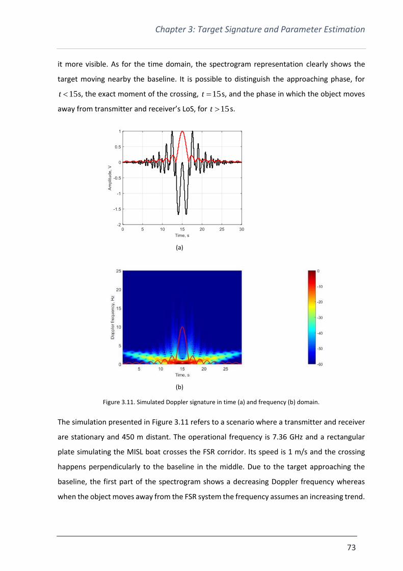
Chapter 3: Target Signature and Parameter Estimation
73
it more visible. As for the time domain, the spectrogram representation clearly shows the
target moving nearby the baseline. It is possible to distinguish the approaching phase, for
15t s, the exact moment of the crossing, 15t s, and the phase in which the object moves
away from transmitter and receiver’s LoS, for 15t s.
(a)
(b)
Figure 3.11. Simulated Doppler signature in time (a) and frequency (b) domain.
The simulation presented in Figure 3.11 refers to a scenario where a transmitter and receiver
are stationary and 450 m distant. The operational frequency is 7.36 GHz and a rectangular
plate simulating the MISL boat crosses the FSR corridor. Its speed is 1 m/s and the crossing
happens perpendicularly to the baseline in the middle. Due to the target approaching the
baseline, the first part of the spectrogram shows a decreasing Doppler frequency whereas
when the object moves away from the FSR system the frequency assumes an increasing trend.

Chapter 3: Target Signature and Parameter Estimation
74
The exact moment in which the target is on the baseline is characterized by a 0 Hz Doppler
frequency and highest value in magnitude. As well as in the time domain, the spectrogram
offers visual information of the target’s cross section. In fact, the central part, which
represents the forward scatter main lobe (FSML) results brighter. Moving away from crossing
point, clearly the return gets weaker as consequence of the FSCS’s side lobes.
(a)
(c) (c)
Figure 3.12. Simulated spectrogram for a target crossing with a speed of 2 m/s (a), 4 m/s (b) and 6 m/s (c).
Figure 3.12 shows how the spectrogram varies for different speeds. The scenario here
presented is the same described for Figure 3.11 with exception of the speed of the target. In
Figure 3.12 object progressively moves at 2 m/s (a), 4 m/s (b) and 6 m/s (c). It is easily
understandable how with the increase of the speed the frequency variation presented in the

Chapter 3: Target Signature and Parameter Estimation
75
spectrogram becomes quicker and consequently the V-shape sharper. In fact, the trend is
proportional to the factor two of the speed: 5 seconds before the crossing the Doppler
frequency is nearly 25.6 Hz in (a), 25 Hz in (b) and 56 Hz in (c).
(a) (b)
(c)
Figure 3.13. Simulated spectrogram for a target crossing the baseline with a crossing angle of 30⁰ in the middle (a), 125 m from Rx (b) and 25 m from Rx (c).
Figure 3.13 shows the effects of the crossing point on the spectrogram. Results for a scenario
in which the target, moving at 2 m/s, crosses with an angle of 30⁰ in different points of the
450 m baseline are here proposed. The crossing happens at 225 m (in the middle of the
baseline) (a), 125 m (b) and 25 m (c) from Rx. These results underline a loss of symmetry when
the target happens to move close to one FSR nodes and not perpendicularly to the baseline.

Chapter 3: Target Signature and Parameter Estimation
76
As in Figure 3.6 (b), Figure 3.13 (b) shows a clear asymmetry, with the left and right branches
of the spectrogram appearing to have different inclinations.
(a)
(b) (c)
Figure 3.14. Simulated spectrogram of a target crossing the baseline in the middle, with a speed of 6 m/s and crossing angle of 15⁰ (a), 30⁰ (b) and 60⁰ (c) at 7.36 GHz
The effects of crossing angle variations are shown in Figure 3.14. The proposes simulated
results are from a scenario similar to the previous ones described where the target moves at
6 m/s, crossing the baseline in the middle with different angles. Making a parallel with the
time domain simulations, the smaller the crossing angle the longer the target will be in the
main lobe. As a consequence of this, Figure 3.14 (a), which represent a crossing at 15⁰ shows
a wide bright area around the actual crossing at 15 seconds. On the other hand, Figure 3.14

Chapter 3: Target Signature and Parameter Estimation
77
(b) and Figure 3.14 (c), 30⁰ and 60⁰ crossing angles respectively, present a narrower main lobe.
Moreover, the angle the target crosses the baseline with affects the concavity of the
spectrogram. In fact, in Figure 3.14 (b) the Doppler frequency assumes a concave slope. As the
crossing angle increases, the spectrogram reaches a nearly straight slope, for a crossing angle
60 ⁰, and a convex one when 90ca . The change of concavity is already visible in Figure
3.14. However, it results more evident for lower frequencies.
Figure 3.15 proposes results obtained in a scenario like the one referring to Figure 3.14. The
only different is that now the transmitted frequency is 1 GHz. The simulated time slot has been
increased to 50 s to offer an easier visualization of the changing concavity.
(a)

Chapter 3: Target Signature and Parameter Estimation
78
(b) (c)
Figure 3.15. spectrogram of a target crossing the baseline in the middle, with a speed of 6 m/s and crossing angle of 15⁰ (a), 30⁰ (b) and 60⁰ (c) at 1 GHz.
3.5 Speed Estimation in Frequency Domain
The understanding of how the target’s motion parameters influence the Doppler signature’s
spectrogram is required to define a method to estimate them.
Remembering that:
tLtRtRt RxTxd
2sinsin ( 3.3 )
with d the Doppler phase shift and considering tL constant, as for a stationary FSR, the
Doppler frequency can be expressed as
cpcaTg
RxTxd xvf
LtRtR
dt
dt
dt
df ,,
2
1
( 3.4 )
Therefore, since ( 3.4 ) is function of target’s speed, crossing angle and crossing point, its
solution would allow the extraction of these parameters and the ability to acquire full
knowledge of target’s trajectory.
In the attempt of estimating the kinematic parameters defining the spectrogram’s slope, the
processing focuses on the extraction of its trend. Thus, given a spectrogram, its brightest
points on the left and right of the crossing time at each frequency are selected. In absence of

Chapter 3: Target Signature and Parameter Estimation
79
clutter deteriorating the quality of the spectrogram, these points correspond to the moving
target. This first step consists essentially in scanning the spectrogram along the y-axis in the
attempt of re-constructing its main trend. The second step of the processing is the calculation
of a second order polynomial fitting of the extracted slope. This would give us a mathematical
equation describing the Doppler frequency variation due to the target’s motion. The
polynomial fitting can then be applied to ( 3.4 ). However, an analytical solution of the formula
is achievable only when the target’s crossing happens in the middle of the baseline and
orthogonally to it [4]. Otherwise, ( 3.4 ) can be solved numerically. Considering the case of a
target crossing the baseline perpendicularly in the middle, which according to the power
budget coincides to the case of lowest target power [5], ( 3.4 ) becomes
4
12
2
1222
2
Ltv
tv
dt
tdf
Tg
Tgdd
( 3.5 )
( 3.5 ) assumes 90ca and 2LxTg . With this assumption, the presented relation is only
function of the target’s speed. An analytical solution of ( 3.5 ) would generate four different
solutions, as following
24/3_12/1_
2
2242,0
22 xvxv
Lfvtfvt TgTgdTgdTg
( 3.6 )
Despite the solution of ( 3.6 ) determines multiple values of speeds, two of them can be
eliminated because having negative sign. Moreover, according to the system application and
the typology of target expected, it is possible to neglect the third solution because of an order
of magnitude different from what expected. Therefore, only one reasonable value of speed is
suitable for the radar application.
Figure 3.16 shows the various steps of the processing. A simulated spectrogram is generated
for an FSR scenario characterized by a 450 m baseline. The target’s speed, crossing point and
crossing angle are 3 m/s, 225 m and 90⁰, respectively. Transmitted frequency is 7.36 GHz.
Working the simulated spectrogram in (a) it is possible to reconstruct the V-shape trend as in
Figure 3.16 (b). Thus, its 2nd order polynomial fitting is calculated. Figure 3.16 (c) presents the
overlap between the isolated spectrogram trend and the determined fitting.
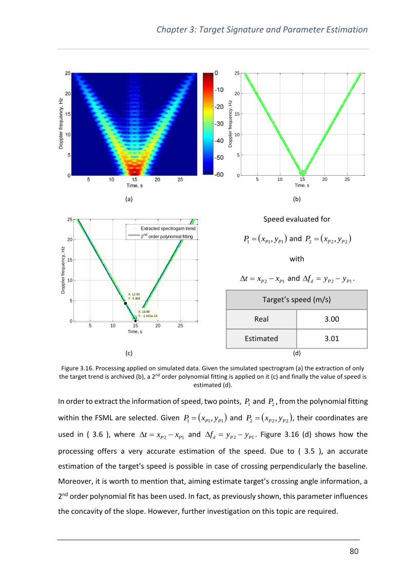
Chapter 3: Target Signature and Parameter Estimation
80
(a) (b)
Speed evaluated for
111 , PP yxP and 222 , PP yxP
with
12 PP xxt and 12 PPd yyf .
Target’s speed (m/s)
Real 3.00
Estimated 3.01
(c) (d)
Figure 3.16. Processing applied on simulated data. Given the simulated spectrogram (a) the extraction of only the target trend is archived (b), a 2nd order polynomial fitting is applied on it (c) and finally the value of speed is
estimated (d).
In order to extract the information of speed, two points, 1P and 2P , from the polynomial fitting
within the FSML are selected. Given 111 , PP yxP and 222 , PP yxP , their coordinates are
used in ( 3.6 ), where 12 PP xxt and 12 PPd yyf . Figure 3.16 (d) shows how the
processing offers a very accurate estimation of the speed. Due to ( 3.5 ), an accurate
estimation of the target’s speed is possible in case of crossing perpendicularly the baseline.
Moreover, it is worth to mention that, aiming estimate target’s crossing angle information, a
2nd order polynomial fit has been used. In fact, as previously shown, this parameter influences
the concavity of the slope. However, further investigation on this topic are required.
5 10 15 20 250
5
10
15
20
25
Time, s
Do
pp
ler
fre
qu
en
cy, H
z
5 10 15 20 250
5
10
15
20
25
X: 14.98
Y: -1.421e-14
Time, s
Do
pp
ler
fre
qu
en
cy, H
z
X: 12.83
Y: 4.308
Extracted spectrogam trend
2nd
order polynomial fitting

Chapter 3: Target Signature and Parameter Estimation
81
Experimental Results
The processing just described, based on the extraction of speed information using the
spectrogram of the Doppler signature, has been tested in a real scenario, in order to prove its
capability.
A single baseline forward scatter radar has been set and the performance of the system
verified. Tx and Rx are shown in Figure 3.17. The equipment was built at the University of
Birmingham and used for several experiments. Being both transmitter and receiver extremely
portable, easy to deploy and contained in waterproof cases, their use is congenial in a
maritime environment. For this reason, all the measurement discussed in this chapter have
been undertaken using this device. Details and specifics about this equipment are presented
in Appendix C.
The transmitter operated in continuous wave at 7.36 GHz and was equipped with a 20 dBi gain
horn antenna.
Results included here were presented in [4] and refer to a maritime measurement set at
Langstone Harbour, UK.
(a) (b)
Figure 3.17. Transmitter (a) and receiver (b) devices.
Figure 3.18 shows a screenshot of the area where the experiment took place, with Tx and Rx
positions clearly marked. Due to the specific location, transmitter and receiver were
positioned one on each side of the harbour. The baseline, visible in Figure 3.18 as a black solid
line, was 298 m long. Data truth was provided using of video cameras and GPS loggers.

Chapter 3: Target Signature and Parameter Estimation
82
Figure 3.18. Google maps view of the measurement at Langstone Harbour.
The main goal of the measurement was to test the performance of our system in detection of
small maritime targets. The same 3 meters two-seater inflatable boat introduced before was
used as a target. It crossed the baseline nearly in the middle using a roughly constant speed
but with different crossing angles. The selected angles the target should have crossed at were
90⁰, 60⁰ and 30⁰. However, due to the current and the difficulties of driving the boat, the
results shown in the following pages refer to 78, 52 and 34 degrees of crossing angle.
The first result is presented in Figure 3.19 . It refers to a situation in which the target crossed
110 m far from the receiver with 78ca ⁰. Figure 3.19 (a) and (b) show clearly the presence
of a target. The clutter contribution is also visible from the spectrogram. However, as all the
measurements were made in a low sea state, the maritime surface does not deteriorate the
performance of the system. Figure 3.19 (c) shows the application of the frequency domain
processing on the proposed spectrogram. The brightest points of Figure 3.19 (b) have been
selected per each frequency and that trend has been approximated to a second order
polynomial fitting. Thus, identified two points on the fitting close to the crossing, the
application of ( 3.6 ) has allowed the estimation of the speed. Since such formula is valid for
an orthogonal crossing, a priori information of the crossing angle has been considered. Thus,
the calculated speed results as the projection of the one obtained with ( 3.6 ), considering the
specific value of ca .

Chapter 3: Target Signature and Parameter Estimation
83
Figure 3.20 presents results at the other two crossing angles. The obtained Doppler signature
and its spectrogram for the MISL boat crossing with an angle of 52⁰ is shown in Figure 3.20 (a)
and (b), respectively. Whereas, Figure 3.20 (c) and (d) propose results for a 34⁰ crossing.
Compering Figure 3.19 and Figure 3.20, it is notable how, in both time and frequency domain
the target signature gets wider with the decrease of the crossing angle. This is an expected
result and matches with the simulations in Figure 3.4 and Figure 3.14. In fact, the smaller is
the target’s crossing angle the longer is the time the target will be in the FSR detection area.
Besides that, comparing the spectrograms in Figure 3.19 (b) and Figure 3.20 (b) and (d), the
concavity of the V-shape slightly changes. Figure 3.19 (b) shows an almost straight slope
whereas Figure 3.20 (b) and (d) start to show a more concave trend.
(a) (b)
(c)
35 45 55 65 75 800
5
10
15
20
25
X: 57.78
Y: 3.125
Time, s
Do
pp
ler
fre
qu
en
cy, H
z
X: 58.63
Y: 0.4222
Extracted spectrogram trend
2nd
order polynomial fitting

Chapter 3: Target Signature and Parameter Estimation
84
Figure 3.19. Doppler signature (a), spectrogram (b) and application of the frequency domain processing (c) for a target crossing at 78⁰.
One more thing that could be noticed, especially in Figure 3.20 (b) and (d), is the presence of
a second, weaker slope following the main one. The reason of this is to attribute to the fact
that in the results shown in Figure 3.20 the MISL boat was crossing pulling an inflatable ball of
having a diameter of 0.65 m. Scattering characteristic of this second target are described in
Appendix C. The presence of the inflatable ball following the main target is notable, but less
visible, also in the time domain.
(a) (b)
(c) (d)
Figure 3.20. Doppler signature and spectrogram for a target crossing at 52⁰ (a and b) and 34⁰ (c and d).

Chapter 3: Target Signature and Parameter Estimation
85
All the presented results in Figure 3.19 and Figure 3.20 show how the target is clearly visible
over the clutter allowing detection and parameter estimation using both time and frequency
domain representation of its crossing.
Table 3.2 reports the values of speed the boat moved during the presented crossings. The
information detected using GPS loggers refers to an average speed along all the period
considered for the crossing. Estimations achieved using the both the described processing
methods, in time and frequency domain are shown to allow comparison. The estimated speed
values matched very well the GPS ones, showing very good accuracy in both cases.
Table 3.2. Real and estimated speed for crossings at 78, 52 and 34 degrees.
Target’s speed (m/s)
Crossing at 78⁰ 52⁰ 34⁰
GPS 3.06 2.90 2.83
Time domain proc. 2.99 3.01 2.80
Freq. domain proc. 3.09 2.69 2.81
3.6 Time and Frequency Domain Approaches in Difficult Scenarios
The last results showed how information of speed can be accurately estimated using both time
domain and frequency domain approaches. This is true when the target is much stronger than
the clutter and therefore both Doppler signature and its spectrogram have clear and
distinctive shapes. This section is dedicated to the comparison of the two methods in case of
difficult targets. We will look at small and big targets and at situations in which the clutter
level is quite high in order to better understand where one processing could help the other
and vice versa.
Small Target
During the course of this PhD project several measurements have been undertaken.
Therefore, we collected signatures from different target. This sub-paragraph focuses on the
performance of our FSR system in case of a small target crossing the baseline. Besides the

Chapter 3: Target Signature and Parameter Estimation
86
inflatable ball already shown in Figure 3.20, which shows a great system performance in
detection of small targets, another example is here given.
(a) (b)
Figure 3.21. Doppler signature (a) and spectrogram (b) of a windsurfer.
Figure 3.21 shows results of a windsurfer crossing the LoS between Tx and Rx during one of
our maritime experiments. The baseline was approximately 300 m and the transmitter
operated at 7.36 GHz. Looking at the Doppler signature, Figure 3.21 (a), the target is hardly
visible, due to presence of clutter and its size whereas, the spectrogram, Figure 3.21 (b), shows
clearly the windsurfer crossing the baseline. Since we are talking about a target of opportunity,
no information about its trajectory are available. However, from the spectrogram it has been
estimated its speed was around 2.20 m/s. Considering the target was moving quite slow, the
wind was not strong and it was an amateur surfer, the estimated speed could be reliable
(highest speeds when taking strong wind are between 15-20 m/s )
Big Target
Another interesting case is the crossing of big targets. In fact, as presented in [1], the radar
results change according to the target’s dimensions and the typology of scattering mechanism
(far/near field). In the specific case here shown, the FSR baseline was 300 m and the
operational frequency 7.36 GHz, as for the previous presented results. The target, shown in
Figure 3.22 (a), was the vessel Arco Dee [6], whose overall length and breadth are 67.7 and 13
m, respectively.

Chapter 3: Target Signature and Parameter Estimation
87
(a)
(b) (c)
Figure 3.22. Doppler signature (b) and spectrogram (c) of the vessel Arco Dee (a).
Figure 3.22 (b) and (c) present the results in time and frequency domain. The Doppler
signature clearly shows how the target, due to its big dimensions, “shadows” completely the
receiver. Therefore, as evident, no direct signal is present anymore. Missing its characteristic
chirp-like form the Doppler signature cannot be used to calculate kinematic parameters. The
spectrogram shows similar features to the time domain representation. In fact, looking at both
Figure 3.22 (b) and (c), the obscuration of the transmitter, with consequent absence of direct
signal, is visible and happens between 50-66.5 s. However, the spectrogram still shows the
final part of its characteristic V-shape, corresponding to the FSCS side lobes. Therefore, the
estimation of speed from the spectrogram is still possible. Furthermore, having an
approximated value of the speed and considering the time the target shadowed the radar, it

Chapter 3: Target Signature and Parameter Estimation
88
is also possible to roughly estimate the length of the vessel. The estimated target’s speed using
the spectrogram is 3.52 m/s. The length of the target can be approximated considering an
interval of time that goes from when the boat enters the FSR detection area ( 47 s) to when
the full shadowing process ends ( 5.66 s). Thus, the length of the target can be approximated
as 64.68475.6652.3 tvD Tg m. Remembering that the real length of the target
is 67.7, such estimation results pretty accurate.
Cluttered Environment
Clutter can influence radar system performance drastically. Therefore, during our maritime
experiments we tried to test our FSR equipment in different situations, with high return from
the surrounding area.
The experiment set up included a single baseline FSR operating at 7.36 GHz. The transmitter
was on the coast whereas the receiver was installed on a ringo, as in Figure 3.23. Thus, Rx was
moving following the sea movement.
Figure 3.23. Receiver node. The Rx is installed on a ringo and equipped with omnidirectional antenna.
Moreover, around 3 dB gain omnidirectional antennas, described in Appendix C, were used in
order to pick returns from all the directions, increasing the level of clutter.
The distance between transmitter and receiver was 350 m and our inflatable boat was used
as a controlled target. Doppler signature and its spectrogram are shown in Figure 3.24. They
refer the case of a crossing in the middle of the baseline with a crossing angle 90ca ⁰. Due
to the receiver swinging according to the sea movement and the use of omnidirectional
antennas, the level of clutter is higher than in the previous results. Consequently, the Doppler

Chapter 3: Target Signature and Parameter Estimation
89
signature does not show its typical chirp-like structure and the presence of target is covered
by the clutter. Similarly, its spectrogram representation presents visual contribution from the
surroundings up to 20 Hz. In this region, the clutter is stronger than the target, not allowing
detection. However, it is still possible to see the characteristic V-shape due to the target
crossing for frequencies above 20 Hz.
(a) (b)
Figure 3.24. Doppler signature and spectrogram in a highly cluttered scenario.
The presence of high clutter deteriorates the usual structure of the Doppler signature, making
the estimation of parameters impossible in this occasion. The spectrogram instead, although
affected by similar issues, still shows a portion of the target slope. Thus, with a focus on the
area above the clutter, the processing in frequency domain is still applicable. The extracted
target’s average speed from the GPS data was 5 m/s. As said the time domain processing was
not able to estimate any useful information whereas the values obtained from the
spectrogram analysis was 4.65 m/s.
3.7 Moving Transmitter/Moving Receiver Target Doppler Signature
A classic FSR configuration with stationary transmitter and receiver can be seen as a specific,
extreme case of moving transmitter/ moving receiver configuration. In this section, the focus
is on the moving TX/ moving Rx FSR configuration. A presentation of how the Doppler

Chapter 3: Target Signature and Parameter Estimation
90
signature looks like and how specific processing enables the estimation of kinematic
parameters in both simulated and real scenarios is here offered.
Figure 3.25 presents a situation in which transmitter, receiver and target are all moving [7].
The scenario and trajectories of all the moving elements are visible in Figure 3.25 (a). The
movements happen in the x-y plane. A motion towards the positive part the y-axis is
considered happening with positive velocity. On the other hand, if the element moves towards
the negative part of the y-axis, its speed has negative sign. As known, due to the motion of
transmitter and receiver, the baseline changes over time and so do motion angles. Therefore,
in order to well describe the scenario and avoid confusion, the geometry is presented with
respect to a reference baseline. In the specific case proposed in Figure 3.25 (a), the reference
baseline is the one on the 0y line, corresponding to the instant 0t . Thus, initial baseline,
crossing points and moving/crossing angles are calculated with respect to this specific
situation.
The transmitter, in solid black line, moves with a speed of 2 m/s along the y-axis. The receiver,
in dashed black line, moves towards the negative part of the y-axis, with velocity equal to -1.3
m/s. The distance to the transmitter, calculated at 0t , is 500 m and the moving angle
60Rx ⁰. The target, in solid red line, moves in the same direction of the receiver. Its velocity
is 6.2Tgv m/s whereas crossing point and crossing angle are 250cpx m and 30Tg ⁰,
respectively. Looking at Figure 3.25 (a), Rx and target crossing angles cannot clearly be
estimated, due to x and y-axis differently scaled. The Doppler signature relative to the
described scenario is presented in Figure 3.25 (b). It has been modelled according to (2.27)
and shaped with the FSCR of a rectangular plate having dimensions similar to the ones of the
MISL inflatable boat.
The motion of Tx, Rx and target defines the way the Doppler signature looks like. As already
said in Chapter 2, it is relevant to remember the critical case of a target staying always on the
baseline, due to a specific combination of the motion of Tx, Rx and target. As a result, the
target Doppler shift would be null so no target Doppler signature would be determined.
Consequently, the system would not be able to detect the target [8]. However, this is an
extremely rare case and the probability of it happening is negligibly small [7], [8].
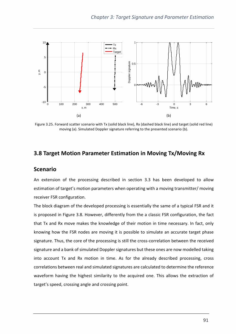
Chapter 3: Target Signature and Parameter Estimation
91
(a) (b)
Figure 3.25. Forward scatter scenario with Tx (solid black line), Rx (dashed black line) and target (solid red line) moving (a). Simulated Doppler signature referring to the presented scenario (b).
3.8 Target Motion Parameter Estimation in Moving Tx/Moving Rx
Scenario
An extension of the processing described in section 3.3 has been developed to allow
estimation of target’s motion parameters when operating with a moving transmitter/ moving
receiver FSR configuration.
The block diagram of the developed processing is essentially the same of a typical FSR and it
is proposed in Figure 3.8. However, differently from the a classic FSR configuration, the fact
that Tx and Rx move makes the knowledge of their motion in time necessary. In fact, only
knowing how the FSR nodes are moving it is possible to simulate an accurate target phase
signature. Thus, the core of the processing is still the cross-correlation between the received
signature and a bank of simulated Doppler signatures but these ones are now modelled taking
into account Tx and Rx motion in time. As for the already described processing, cross
correlations between real and simulated signatures are calculated to determine the reference
waveform having the highest similarity to the acquired one. This allows the extraction of
target’s speed, crossing angle and crossing point.
0 100 200 300 400 500-10
-5
0
5
10
x, m
y, m
Tx
Rx
Target
-6 -3 0 3 6
0
0.5
1
Time, s
Do
pp
ler
sig
na
ture

Chapter 3: Target Signature and Parameter Estimation
92
Results of such processing are shown in Figure 3.26. The investigated case refers to a situation
where Tx, Rx and target moves as in Figure 3.25 (a). In Figure 3.26 (a), the Doppler signature
modelled with the MISL boat RCS is overlapped to the reference signature determining the
highest value of cross-correlation. The reference signatures have been shaped with a
Hamming window. The difference between the autocorrelation of the modelled signature and
its cross correlation with the reference signature is shown in Figure 3.26 (b). In order to
achieve a more realistic scenario, the values of speed, crossing angle and crossing point
defining the modelled signature have not been included in the ranges of values used to create
the reference signatures. Consequently, results in Figure 3.26 show two waveforms very
similar but not overlapping.
(a) (b)
Figure 3.26. Modelled with RCS (black line) and simulated (red line) Doppler signatures (a). Comparison between the autocorrelation of the modelled signature (black line) and its correlation with the simulated
one (red line) (b) [7].
The processing performance is summarized in Table 3.3 where the motion parameters of the
simulated Doppler signature are compared to the estimated ones. Despite, as said above, the
real values of parameters were not included in the ones used to calculate the reference
signatures, results show a very good match between real and estimated parameters. Results
in Table 3.3 would coincide if the correct values of speed, crossing angle and crossing point
are used in bank of filters generated during the processing.
-6 -3 0 3 6-1
-0.5
0
0.5
1
Time, s
Do
pp
ler
sig
na
ture
S
RO
Sim,jm,km
2000 3000 4000-25
-20
-15
-10
-5
0
Sample
Co
rre
latio
n, d
B
S
RO*S
RO
SRO
*Sim,jm,km

Chapter 3: Target Signature and Parameter Estimation
93
Table 3.3. Processing performance on simulated signature.
Speed (m/s) Crossing angle (⁰) Crossing point (m)
Simulated -2.6 30 250
Estimated -2.4 35 255
Experimental Results
Experimental results collected during a NATO SET-192 maritime measurements campaign in
Livorno, Italy are here presented. Records have been acquired at low sea state of 2 or lower
on the Douglas scale [7], [8].
The aim of our experiment was to prove the capability, in terms of detection and parameters
estimation, of an FSR system having at least one node moving. In this experiment, the same
maritime equipment previously presented and described in Appendix C, has been used. A
single node FSR configuration has been set. Transmitter is shown in Figure 3.27 (c). It was
operating at 7.36 GHz (CW) and was installed on the Italian shore. The high deployability of
our system allowed the receiver, in Figure 3.27 (b), to be installed on a moving sailing boat, as
shown in Figure 3.27 (a). For security reasons imposed by the Italian navy, the moving platform
with the receiver was not allowed to go too far from the coast. Therefore, despite the system
capability to operate at bigger distances, the baseline length was between 400-600 m.
(a) (b) (c)
Figure 3.27. Sailing boat used as moving platform for our receiver (a), Rx side with receiver in the pelicase (b) and Tx side (c).

Chapter 3: Target Signature and Parameter Estimation
94
Our inflatable boat operated as controllable maritime target, moving between transmitter and
receiver. Video cameras and GPS loggers were used to provide data truth and record receiver
and target trajectories.
(a)
(b) (c)
Figure 3.28. FSR scenario with receiver and target moving in the same direction (a), acquired and estimated target Doppler signature (b) and comparison between the autocorrelation of the recorded Doppler signature
and its correlation with the extracted reference signature(c) [7].
Figure 3.28 shows a case in which receiver and target are moving in the same direction. Figure
3.28 (a) clearly pictures the position of transmitter, receiver and target and their trajectories.
The black line represents the reference baseline. Its length is 515 m. According to GPS data,
the receiver moved with a speed of 1.9 m/s and with an angle of 110⁰. The target crossed the
reference baseline 274 m far from the Tx, with an angle 105ca ⁰ and a speed of 2.5 m/s.
This scenario could introduce some limitation in the performance of the systems. In fact, since
Rx and target move towards the same direction, the resulting target speed would decrease.
-6 -3 0 3 6-1
-0.5
0
0.5
1
Time, s
Do
pp
ler
Sig
na
ture
S
RO
Sim,jm,km
2000 3000 4000-25
-20
-15
-10
-5
0
Samples
Co
rre
latio
n, d
B
S
RO*S
RO
SRO
*Sim,jm,km

Chapter 3: Target Signature and Parameter Estimation
95
This could deteriorate the detection performance in case of either high clutter or target
maintaining its position nearly on the baseline.
Figure 3.28 (b) and (c) present results from the processing. Figure 3.28 (b) shows in black the
acquired signature and in red the extracted reference waveform. Differences between
autocorrelation of the real signature (in black) and its correlation with the extracted signal (in
red) are proposed in Figure 3.28 (c).
A case in which Rx and target move in opposite direction is shown in Figure 3.29. Transmitter,
receiver and target position acquired by GPS loggers are visible in Figure 3.29 (a). The
reference baseline, black solid line, is 488 m. Rx moved with a speed of 2 m/s almost
perpendicularly to the reference baseline. The target moved in opposite direction. Its crossing
point, crossing angle and speed were 269cpx m, 75ca ⁰ and 6.2Tgv , respectively. As
for Figure 3.28, Figure 3.29 (b) and (c) show the results from the processing. Table 3.4 shows
the results of the processing applied on the proposed data. As visible, the estimation of speed
results quite accurate whereas a higher error is found in the estimation of crossing angle and
crossing point. This is partially due to the fact that all the motion parameters are assumed
constant within the visibility time. Moreover, the speed is the parameter that influences the
target signature the most whereas different combinations of crossing angles and crossing
points could determine similar results in terms of signature trend.
(a)

Chapter 3: Target Signature and Parameter Estimation
96
(b) (c)
Figure 3.29. FSR scenario with receiver and target moving in opposite direction (a), acquired and estimated target Doppler signature (b) and comparison between the autocorrelation of the recorded Doppler signature
and its correlation with the extracted reference signature(c) [7].
Table 3.4. Processing performance on real data.
Scenario Speed (m/s) Crossing angle
(⁰)
Crossing point
(m)
Same direction Acquired 2.5 105 274
Estimated 2.2 120 150
Opposite
direction
Acquired -2.6 75 269
Estimated -2.9 125 120
As visible looking at Table 3.4, it is possible to extract information of the direction of the target,
represented by the speed sign. Due to its symmetries, a typical FSR is not able to determine
the direction the target comes from. These symmetries are broken with the introduction of Tx
and Rx motion. Therefore, the knowledge of the motion of the FSR nodes allow to identify the
direction the target is moving to.
Proposed results show good achievements even in a condition of moving Tx/moving Rx.
However, the specific tested scenario does not look extremely affected by Doppler spread and
clutter Doppler shift, which has been underlined as possible limiting factors for such FSR
configuration.
-6 -3 0 3 6-1
-0.5
0
0.5
1
Time, s
Do
pp
ler
sig
na
ture
S
RO
Sim,jm,km
2000 3000 4000-25
-20
-15
-10
-5
0
Samples
Co
rre
latio
n, d
B
S
RO*S
RO
SRO
*Sim,jm,km

Chapter 3: Target Signature and Parameter Estimation
97
3.9 Conclusions
The entire chapter has focused on the description of the Doppler signature, the possibility to
detect a target and the estimation of kinematic parameters. The target phase waveform has
been shown in both time and frequency domain, giving particular interest to how it is
influenced by parameters such as transmitting frequency, target’s speed, crossing angle and
crossing point. The initial part of the chapter has been dedicated to the FSR target signal in
case of stationary transmitter and receiver. In fact, a full understanding of the stationary FSR
scenario is necessary to then proceed to the moving Tx/moving Rx configuration.
Information regarding target detection and parameter estimation in FSR has been provided
using the following approach:
• presentation of the signature and the effects motion parameter have on it;
• introduction of a processing enabling the estimation of kinematic parameters and
show its results on simulated data;
• proposition of results from experimental campaigns and show the performance of the
processing on real data.
Two different techniques for analysis of stationary FSR data have been introduced. The first
one, operating in time domain, is a processing developed and used by researchers at the
University of Birmingham to estimate motion parameters using a bank of reference
signatures. The second one, operating in frequency domain, is a technique developed during
the course of this PhD project to support and/or overcome some limitations of the pre-existing
algorithm.
The final part of the chapter has focused on the moving Tx/moving Rx FRS. A new way to
describe and model the Doppler signature and the radar cross section has been developed, in
order to achieve description of the received signal and extract target’s motion information
from it. Mathematically, these models are quite similar to the already existing ones. In fact,
the main difference is that they take into account transmitter and receiver motions. However,
they represent an evolution with could allow future use of the FSR technology in a totally
different and challenging way. In addition to that, an evolution of the time domain processing
used to extract target’s kinematic information has been developed and introduced. The

Chapter 3: Target Signature and Parameter Estimation
98
presentation of the results has followed the same structure used for the first part of the
chapter: an example of simulated Doppler signature for the moving ends FSR has been shown
together with the description of the processing and its performance on both simulated and
real data.
The methods described in this chapter have shown some benefits and drawbacks. A summary
of these is proposed below.
• Time domain processing
o Able to estimate target’s speed, crossing angle and crossing point
o Time consuming because it relies on a bank of filters
o Dependent of the chirp-like structure of the Doppler signature. Thus, it could
not perform well in difficult scenarios such as highly cluttered enviroment
• Frequency domain processing
o Able to estimate target’s speed. Crossing angle and crossing point estimation
to be further investigated.
o More robust to clutter
o Useful as support for the time domain processing
• Time domain processing for moving Tx/Rx FSR
o Able to estimate target’s speed, crossing angle and crossing point
o Requires knowledge of Tx and Rx motions
o Performance can be influenced by Doppler shift and clutter Doppler spread

Chapter 3: Target Signature and Parameter Estimation
99
3.10 Bibliography
[1] M. Gashinova, L. Daniel, V. Sizov, E. Hoare, and M. Cherniakov, ‘Phenomenology of Doppler forward scatter radar for surface targets observation’, Sonar Navigation IET Radar, vol. 7, no. 4, pp. 422–432, Apr. 2013.
[2] H. L. Van Trees, K. L. Bell, and Z. Tian, Detection estimation and modulation theory, Second edition. Hoboken, N.J: John Wiley & Sons, Inc, 2013.
[3] F. E. Nathanson, J. P. Reilly, and M. Cohen, Radar design principles: signal processing and the environment, Second Edition. Edison, NJ: Scitech Publishing, 1999.
[4] A. De Luca, M. Contu, S. Hristov, L. Daniel, M. Gashinova, and M. Cherniakov, ‘FSR velocity estimation using spectrogram’, in 2016 17th International Radar Symposium (IRS), 2016, pp. 1–5.
[5] V. Sizov, M. Cherniakov, and M. Antoniou, ‘Forward scattering radar power budget analysis for ground targets’, Sonar Navigation IET Radar, vol. 1, no. 6, pp. 437–446, Dec. 2007.
[6] ‘Vessel details for: ARCO DEE (Dredger) - IMO 8902917, MMSI 232003387, Call Sign MMWE3 Registered in United Kingdom | AIS Marine Traffic’, MarineTraffic.com. [Online]. Available: http://www.marinetraffic.com/en/ais/details/ships/shipid:182975/mmsi:232003387/imo:8902917/vessel:ARCO_DEE. [Accessed: 17-Aug-2017].
[7] A. De Luca, L. Daniel, M. Gashinova, and M. Cherniakov, ‘Target parameter estimation in moving transmitter moving receiver forward scatter radar’, in 2017 18th International Radar Symposium (IRS), 2017, pp. 1–7.
[8] A. De Luca, L. Daniel, K. Kabakchiev, E. Hoare, M. Gashinova, and M. Cherniakov, ‘Maritime FSR with moving receiver for small target detection’, in 2015 16th International Radar Symposium (IRS), 2015, pp. 834–839.

Chapter 4: Clutter in FSR
100
Clutter in FSR
Glossary of Abbreviations
CW Continuous Wave
FSR Forward Scatter Radar
MISL Microwave Integrated System Laboratory
PDF Probability Density Function
PSD Power Spectral Density
RCS Radar Cross Section
Rx Receiver
Tx Transmitter
UHF Ultra-High Frequency
VHF Very High Frequency
4.1 Introduction
In a forward scatter radar (FSR) configuration with transmitter (Tx) and receiver (Rx) installed
on moving platforms, the contribution of the surrounding environment could influence the
performance of the system heavily [1]. In fact, as explained in Chapter 2, the motion of the
nodes introduces Doppler shift and clutter Doppler spread which, depending on their
characteristics, could decrease the probability to detect targets. Therefore, an investigation
on clutter has been conducted in order to understand characteristics and features of its
deteriorating effects on an FSR system.
In the previous chapter, results from maritime FSR trials with moving receiver have been
proposed. Despite the motion of the receiving node, the acquired signal was not affected by
clutter and both detection and parameter estimation have been possible. This can be
Chapter 4: Clutter in FSR
101
associated to the fact that the maritime surface, in absence of big waves, does not represent
a big limitation for an FSR system. Differently, the radar performance could be highly
deteriorated when considering vegetation clutter, such as the presence of trees and bushes.
For this cause and also because, due to logistic reasons, it would have been easier to
undertake measurements in areas nearby the University of Birmingham, vegetation clutter
has been investigated.
The following pages are divided in three main parts:
• initially, a brief introduction of ground clutter is proposed. A good understanding of its
features and behaviour has been fundamental for our purpose;
• the central part of the chapter focuses on the description of an adaptable model to
simulate vegetation clutter in different scenarios. The acquired knowledge on
vegetation characteristics has been a starting point to develop a model describing
vegetation environment. Such model has taken inspiration from an already published
concept used to simulate returns from ground clutter [2], [3]. However, this new
approach has been designed to be extremely flexible, easily adaptable to different
scenarios and suitable for classic and moving ends FSR.
• the last part of the chapter is dedicated to the presentation of experimental results
obtained during different measurement trials. The investigation has focused on
understanding how different operational frequencies, nodes’ speeds and trajectories
influence radar performance. In addition to that, simulations of such measurements
have been generated to test the developed model. In fact, being the clutter extremely
variable and strongly dependent on location and composition of the vegetation, a
description of its features is extremely challenging. In this case, the presence of a
reliable model could simplify the problem.
The personal contribute to this chapter includes:
• investigation of vegetation behaviour and development of a flexible model simulating
radar environmental returns. It has been necessary to understand how to model
different surfaces and how to simulate the motion of trees. The developed approach
allows is highly adjustable and allows to locate each vegetation scattering element

Chapter 4: Clutter in FSR
102
(surface, bush or tree) and to set Tx and Rx position in time. Therefore, it is extremely
useful to describe a stationary of moving ends FSR;
• clutter contribution analysis. Several simulated scenarios have been tested using the
developed approach to understand how the clutter influences the system
performance. Particular interest has been given to radar operational frequency and
Tx/Rx trajectories;
• several experimental campaigns have been undertaken to quantify how the clutter
affects the radar. It has been necessary to understand the effect of transmitting
frequency, node trajectory and speed on the system. Experimental and simulated date
have been compared showing a good match between them.
4.2 Land Clutter
Clutter has a strong contribution on bistatic radar’s performance. When operating in
continuous wave (CW) as already seen in Chapter 2, clutter returns interfere with target ones,
challenging the possibility to detect desired objects [1], [4]. Therefore, echoes from the
surrounding environment are the main limiting factor [3].
Land clutter can be seen as a composition of terrain surface and foliage contributes, with the
former strictly related to the characteristics of the surface and the latter to the kind of
vegetation on it. In a conventional FSR system the interest is only on foliage returns [2], [3],
[5]. In fact, the Doppler signature would show only contributes related to moving elements
surrounding the radar. However, when considering a configuration with transmitter and
receiver installed on moving platforms, their motion would enable the reception of
contributes from stationary elements too. Thus, for our purpose both surface and vegetation
have been considered.
As well known, [4], [6]–[8], surface clutter is strongly dependent on:
• roughness of the surface, in terms of wavelength;
• kind of surface, if concrete, rural, rocks, with vegetation etc.;
• frequency;
• incident angle;

Chapter 4: Clutter in FSR
103
• scattering angle;
• out-of-plane angle.
An accurate statistical description of surface clutter is extremely difficult because of the
dependence on these listed parameters. Moreover, many other factors influencing the
scattering mechanism of the terrain, such as an unclear relationship between the kind of
surface and its scattering properties, the presence of obstacles, moister in the soil and snow,
make this a challenging task [7]. Thus, clutter features have been mainly determined through
several trial campaigns aiming to confirm an average behaviour of surface clutter in specific
conditions. As for every target, a way to define how unwanted echoes influence a radar system
is through its radar cross section (RCS). For surface clutter this means measure the energy
scattered from a clutter cell in the direction of the receiver [9]. Since this parameter is function
of terrain composition, frequency and geometry, most of the material available in literature
refers to the monostatic case. Not much data is accessible for bistatic configurations [7], [9]–
[12].
Figure 4.1 shows the bistatic geometry for a point-like clutter. , i , s and are the
bistatic, incident, scattering and out-of-plane angles, respectively. Most of the data available
has been measured in condition of in-plane configuration, with Tx, Rx and scattering surface
point lying on the same plane.
Figure 4.1. Bistatic geometry for a point-like clutter.

Chapter 4: Clutter in FSR
104
Surfaces are characterized by , which is the normalized reflectivity parameter and defines
the RCS. Thus, considering that, in monostatic clutter the RCS is modelled as follow
iCM sin ( 4.1 )
As intuitive, being Tx and Rx co-located, the radar cross section in the monostatic geometry
depends only on the terrain features and incident angle.
The bistatic scattering model for land clutter is obtained using a variation of the monostatic-
bistatic equivalent theorem [9]. Such theorem, introduced by Crispin and Siegel and slightly
modified by Kell [9], [13], [14], applies on pseudo-monostatic regions and says that the bistatic
RCS of a smooth and perfectly conducting object is equal to the monostatic one calculated on
the bisector of the bistatic angle. Hence, the bistatic clutter RCS can be expressed as
21sinsin siCB ( 4.2 )
Values of can be determined using collected data. Figure 4.2 shows a table extracted by [7]
where the average values of are proposed for different surfaces and at different frequency
bands.
Figure 4.2. Average land clutter return in decibel. i sin0 with 15i ⁰ to 70 ⁰ grazing [7].
Due to the enormous different combinations of all parameters affecting the clutter RCS, not
much data is available for out-of-plane configurations [9].
The foliage clutter instead is connected to the presence of bushes, branches and foliage
swinging as results of wind blowing. Thus, it depends on the wind strength and on the period
of the year, considering many trees during autumn/winter do not have leaves. In a FSR

Chapter 4: Clutter in FSR
105
configuration, swinging bushes and trees introduce a similar shadowing effect than a normal
moving object. Therefore, such kind of environmental elements can be treated in the same
way of target, with their RCS calculated similarly.
4.3 Clutter Model
With the attempt to investigate the effect of clutter on a FSR system having transmitter and
receiver installed on moving platforms, a specific model to simulate the environment
surrounding the radar device has been developed.
As previously said, an initial model to describe vegetation clutter in FSR was presented in [2],
[3]. In both papers, a combination of swinging points was used to replace the effect of foliage
moving under wind blowing conditions. However, the defined model applied to a static
forward scatter situation. Differently from [2], [3], during my PhD I have worked on developing
a model that could be used to describe extensive areas of land with vegetation. Such approach
can be used to simulate radar returns in case a FSR having Tx and Rx installed on moving
platforms.
This section focuses on the description of a model to represent vegetation clutter considering
the main elements that influence a forward scatter radar system with nodes able to move.
The complex task of describing vegetation clutter can be break down in two main components:
influence of the surface and influence of vegetation.
Simulated Surface
The surface has been thought of as a composition of multiple point-like scattering elements
having a specific RCS. Therefore, in the developed model the terrain is simulated as a
rectangular grid of desired dimensions. The size of such grid is defined taking into account Tx,
Rx and target positions in time, making sure they lie inside the simulated surface. In fact, this
should provide a more realistic result. Figure 4.3 shows the grid, which defines the surface
scattering points, and the FSR transmitting and receiving nodes lying on it.
The main difficulty encountered during the development of a surface model has been the
evaluation of the radar cross section to assign to each scattering point. In fact, instant by
instant, considering the motion of Tx and Rx, the majority of the points are out of the

Chapter 4: Clutter in FSR
106
transmitter-receiver plane. As said above, not much material regarding scattering mechanism
of out-of-plane surface points is available and the few available refer to very specific
experimental campaigns [10]–[12].
Figure 4.3. FSR geometry with ground surface replaced by a rectangular grid.
Therefore, in order to identify the RCS value to assign time by time to each point, ( 4.2 ) has
been used. This means the scattering mechanism has been assumed to happen in-plane for
all the surface points at every instant. As reported in [9], out-of-plane CB is lower than its in-
plane version, even if for angles close to the in-plane scenario such discrepancy is not extreme.
Thus, CB calculated in in-plane conditions can be seen as the upper limit of the out-of-plane
version. Being the main purpose of this investigation aiming to understand the effects of the
environment on a having moving transmitter and receiver FSR system, such assumption on
the surface RCS is acceptable. In fact, it represents the most unfavourable scenario.
Simulated Vegetation
The vegetation covering a land surface is usually a mix of bushes and trees. Several studies
have been undertaken in literature to describe plants in terms of branch distributions and
phyllotaxis, leaves’ arrangement on a plant. Some approaches based their foundations on
mathematical biology, some others on optimization mechanisms, such as the maximization of
light interception [15]–[21].
This section presents a simplified approach aiming to describe vegetation. Such model, based
on the one already proposed in [2], [3], can be used to represent complex areas with
vegetation and allows to investigate a moving Tx/ moving Rx FSR scenario.

Chapter 4: Clutter in FSR
107
Figure 4.4 shows the way a bush has been thought of in order to be implemented. According
to the developed model, such vegetation element is composed by several branches having
origin in the bottom centre of the bush itself, which is considered as its root. Each branch is
made by a sequence of scattering points. Trying to keep the model as simple and functional
as possible, leaves and their motion have not been taken into account. In fact, the presence
of leaves would introduce a huge amount of extra scattering points, increasing tremendously
the algorithm computational cost. Moreover, for the ranges of frequencies tested and
applications thought, the presence of leaves can be initially omitted. Further studies could
consider the introduction of these extra scattering elements to investigate more precisely the
impact of vegetation in FSR.
Figure 4.4. Bush concept. From reality to simplified model.
Let us discuss in detail the steps used to create a single branch. The first thing to do is to define
the number of branches we desire to have the bush made of. This can be done either selecting
a fixed number of branches or generating such amount with a statistical distribution, more
suitable in case of simulation of multiple vegetation elements. Given a branch, its length Bl
needs to be defined. The majority of the bushes could be considered composed by branches
having similar length, either because they are cut in symmetrical ways or because they grow
uniformly. Thus, the length of the branches of each bush can be generated using a Gaussian
distribution around a set mean value Bm and with a desired variance B~ . The scattering points
on a single branch are taken with a step equal to the wavelength. Thus, each branch contains
as many scattering points as the times its length Bl is multiple of , plus its extremity. In fact,
the extreme point of a branch is always considered as scattering element. For example, if
operating at 1 GHz ( 3.0 m) and having 2 branches b1 and b2 whose length is 0.60 m and

Chapter 4: Clutter in FSR
108
0.75 m, respectively the former will have two scattering points (at 0.30 and 0.60 m from the
origin) whereas the latter will have three scattering points (at 0.30, 0.60 and 0.75 m from the
origin). For simplicity, the branch is initially thought lying on the x-y plane, with its origin in (0,
0) and stretching along the x axis (see Figure 4.5 (a)). As suggested in [2], [3] the motion of a
branch can be associated to the pendulum’s one.
(a) (b)
Figure 4.5. Single branch swinging in the x-y plane (a) and its rotation in a 3D space (b).
Figure 4.5 (a) summarizes the swinging motion of a single branch. As reported, a Bl long
branch is considered made of two scattering points ),(1 1010 yxP and ),(2 2020 yxP . 0ix and
0iy represent the coordinates of the scattering point on the x and y axis. is the amplitude
of the swing in terms of angle; it depends on the branch’s thickness and wind’s strength.
However, assuming all the branches similar in terms of robustness and flexibility, results
just function of the wind. 2cos00 iix xxA and sin0iy yA are the amplitudes of
oscillation in the x and y axis, respectively. Thus, the movement visualized in Figure 4.5 (a) can
be described mathematically as follows

Chapter 4: Clutter in FSR
109
00
00
sin
2cos
T
tAyty
T
tAAxtx
yii
xxii
( 4.3 )
with ix and iy the position of the ith scattering point on the coordinate axis. wind
B
F
lT is the
swinging period, with windF the wind strength. From Figure 4.5 the period of the motion along
the x axis appears to be half the one on the y axis. 0 is the initial phase. It is calculated for
each branch using a Gaussian distribution so that all the scattering points of a single branch
share the same initial phase and all the branches have a similar but slightly different one. The
mean value of such distribution is uniformly distributed between and , to guarantee
different initial phase for different bushes. Once the branch has been created and its
movement generated, the next step is to position such branch in the 3D space, in order to
generate a bush-like structure. Thus, a rotation along the z axis first and along the y axis then
is implemented. The rotational matrixes used to move the scattering points from the x-y plane
to a x-y-z space are proposed in ( 4.4 ).
100
0cossin
0sincos
zz
zz
zR
yy
yy
yR
cos0sin
010
sin0cos
( 4.4 )
z and y are the rotational angles on the z and y axis respectively for each branch. The
former is uniformly distributed between and whereas the latter between and 0 ,
so it allows rotations only towards the positive side of the z axis.
Figure 4.5 (b) shows how such described matrixes affect the position of the branch. Once
placed the branch in the 3D space, it can be translated in the position chosen as origin for the
bush. The relation that allows to calculate the coordinates of a scattering element taking in
consideration its initial position, the rotational matrixes and the bush root is the following

Chapter 4: Clutter in FSR
110
R
R
R
i
i
i
zy
z
y
x
tz
ty
tx
RR
tz
ty
tx
( 4.5 )
Rx , Ry and
Rz are the x, y and z coordinates of OP , the bush’s root point.
Before to continue with a more complex and less controllable scenario, it is interesting to
understand how a single scattering point affects an FSR system.
The following simulations refer to the case of a stationary FSR system. The baseline is 100 m
and Tx operates at 1 GHz. The selected point-like target is the extremity of a 0.5 m branch. T
is 5 seconds and 30 ⁰. Ultimately, 0 , z and y are all null. The element’s motion in time
calculated according to ( 4.4 ) is proposed in Figure 4.6.
(a)
(b)
Figure 4.6. Scattering point position along the x (a) and y (b) axis.
Trying to understand and test the proposed model, several simulations have been run shifting
the origin of the branch. Four different values of OP have been used. Such points have been
chosen in order to compare the cases of branch crossing and not crossing the isophase regions.

Chapter 4: Clutter in FSR
111
Thus, the distances from the baseline at which the change of isophase regions occur have been
calculated. Figure 4.7 (a) shows the intersections between the scatterer Doppler signature’s
phase and the phase values defining the isophase contours. This has allowed the
determination of the distance from the centre of the baseline necessary to reach a different
isophase region. On the base of that, OP has been chosen:
• within the first isophase region, black triangle in Figure 4.7 (b);
• on the edge of the first, second and third isophase region and able to cross it;
respectively red, green and blue triangles in Figure 4.7 (b).
The Doppler signature of the point like target has been calculated for all the above listed
scenarios, Figure 4.7 (c). The colours of the signatures follow the ones used in Figure 4.7 (b) to
indicate the various branch origins. As expected, when the scattering element crosses an
isophase region during its swinging motion another harmonic is produced. This is clearly visible
focussing on the red, green and blue waveforms in Figure 4.7 (c). On the other hand, the black
waveform does not produce a similar effect, since the scattering point stays in the same
isophase region during all its movement. A similar consideration is also presented in [2],
confirming the simulation results.
(a) (b)

Chapter 4: Clutter in FSR
112
(c)
Figure 4.7. Influence of the scattering point of origin. Doppler signature phase and isophase regions (a), isophase regions and origins of the branch (b) and scatterer Doppler signature for the different origins (c).
Repeating the steps described before for the desired number of branches it is possible to
model a bush-like structure. In such case, all the branches will share the same origin, but will
have different length, although similar since generated through a Gaussian distribution, and
different position in space due to the different rotation angles z and y .
For a more complete description of a vegetation scenario, along with the bush model it has
been necessary to simulate trees as well. In fact, the University of Birmingham area is a very
green zone full of vegetation. Therefore, the measurement locations would have presumably
been full of trees too. As stated already before, since our aim is not to describe clutter in the
most accurate way but to identify the limitations introduced by it, it has been decided to
model trees in a simple way, as rectangular form extending along the vertical direction.
Therefore, the complex task of modelling a tree has been to break down in simpler steps using
the concept represented in Figure 4.8. In fact, such element can be simulated as a sum of
bushes one on each other, each of them made by a sum of branches composed, in turn, by
several scattering points. Using this criterion and having in mind the way to simulate a bush,
the development of a tree is straightforward. In fact, the only parameters to define are the
ones describing the structure of the tree: height, maximum branch length and thickness (in
terms of number of branches).

Chapter 4: Clutter in FSR
113
Figure 4.8. Tree structure.
The number of bushes forming a single tree is obtained dividing its height for the maximum
vertical dimension of a bush, which is equal to two times the maximum branch length. The
height of the tree’s trunk is defined as a portion of its vertical length and is also the z-axis
origin of the first bush composing the tree. The second one has its origin on top of the first
one and so on, creating a pile of vertical bushes. All these elements are formed in the way
previously described with exception of y which in this case is uniformly distributed between
and .
Doppler Signature Creation
The vegetation elements described above are the elementary pieces representing the
surrounding environment in the developed simulations. In fact, it is possible to model different
scenarios, creating a replica of the ones we are interested in, just by inserting the desired
surface and number of trees and bushes in the specific positions. In such way, a virtual
representation of a real environment is obtained. Once created the scenario, it is necessary to
define the position of transmitter and receiver and define their motions. As for a target, the
two-ray path approach, described in Chapter 2, has been used to calculate the radar
environment received signature.
Following such approach, the environment Doppler signature is obtained as
j bushji treeisurfLSTOT uuuuu __ ( 4.6 )
where LSu is the leakage signal and surfu , treeiu _ and bushju _ are contributes from the surface,
tree and bush, respectively.

Chapter 4: Clutter in FSR
114
Such signal has been adapted to replicate the one received by the experimental equipment
used. Therefore, the received calculated power has been modelled using the Rx calibration
curve. More information is included in Appendix D.
Figure 4.9. Simulated scenario of a real area nearby our university building.
Figure 4.9 shows the overlap between a real scenario and its simulated one. It refers to one
of the experiments undertaken during this PhD project to investigate the effect of a receiver
moving along the baseline. The full area (purple grid) with trees (green asterisks indicating
their roots) has been simulated. Also, position and motion of Tx and Rx have been simulated
to replicate the exact measurement. The experiment and its results are presented in detail in
the following pages.
A (130x82) m grid (purple structure in Figure 4.9) having 1-sqm cells has been implemented
to simulate the ground surface. For simplicity, it has been assumed flat and scattering as an
average open wood area. Thus, as from Figure 4.2, 16 dB. Dense and high trees compose
the vegetation around the selected area shown in Figure 4.9. Trying to mimic the location,
shrubs have been placed on two rectangular areas of (44x38) m and (36x48) m respectively.
Their selected roots are shown with green asterisks in Figure 4.9. Assumed all the trees having
similar features, their maximum height has been set equal to 20 m. Maximum branch length
and swinging period were 4 m and 2 seconds, respectively. The amplitude of oscillation for

Chapter 4: Clutter in FSR
115
each branch has been considered proportional to the wind strength (the stronger the wind
the wider the oscillation). However, it has been also taken into account that too big oscillations
would break the branch. Thus, an oscillation of 50⁰ has been set a maximum allowed flection.
Each bush-like element used to build the tree in the vertical direction had 30 branches,
creating a well dense shrub. The distance between the roots of adjacent trees is equal to the
maximum branch length. Positions of transmitter and receiver in Figure 4.9 are indicated by
the blue and red circles, respectively. Moreover, the black line explains the Rx’s trajectory.
(a) (b)
(c) (d)
Figure 4.10. Simulated clutter at 173 MHz for the scenario shown in Figure 4.9. Doppler signature and spectrogram for the stationary case, (a) and (b), and for the case with Rx moving at 6.55 m/s, (c) and (d).
Figure 4.10 presents results at 173 MHz from the simulated scenario in case of stationary and
moving receiver. Doppler signature and spectrogram for a classic FSR situation are shown in
(a) and (b), respectively. On the other hand, (c) and (d) show time and frequency domain
signatures for the receiver moving with a speed of 6.55 m/s. The comparison between the
0 50 100 150 200 250-0.6
-0.5
-0.4
-0.3
-0.2
-0.1
0
0.1
0.2
0.3
0.4
Time, s
Re
ce
ive
d a
mp
litu
de
, V
olt
0 1 2 3 4 5 6 7 8-1
-0.8
-0.6
-0.4
-0.2
0
0.2
0.4
Time, s
Re
ce
ive
d a
mp
litu
de
, V
olt

Chapter 4: Clutter in FSR
116
results shown in Figure 4.10 suggests the increase of clutter strength due to the moving
receiver. In fact, as visible from the spectrograms, the contribution of the surrounding area is
below 1 Hz in case of stationary receiver whereas it increases up to around 7/8 Hz when the
receiver moves at 6.55 m/s.
To understand the law ruling the increase of clutter level in our specific scenario, an analysis
on simulated signals has been undertaken. Therefore, considering the geometry in Figure 4.9,
the effects of receiver speed and transmitted frequency on clutter Doppler shift have been
investigated. Power spectral densities (PSDs) of the received signatures calculated using the
TRP model are shown in Figure 4.11. The curves refer to the case of receiver moving as in
Figure 4.9 at 1, 3 and 9 m/s. The picture clearly shows a frequency contribution limited by the
Doppler shift, which creates an evident sharp edge. The peaks visible in Figure 4.11 correspond
to the values 𝑓𝐷𝑆 = 𝑣𝑅𝑥/𝜆. Doppler spread due to the presence of swinging vegetation
increases the frequency contributes below the Doppler shift. Therefore, the figure does not
show only peaks at 𝑓𝐷𝑆 but rather pedestals limited by the Doppler shift values.
Figure 4.11. PSDs at 173 MHz calculated for different Rx speeds without taking into account the receiver’s calibration curve.
When applying the receiver’s calibration curve the PSDs change: the curves are smoothed,
without the previously noticed sharp edge, and second peaks at higher values than the ones
in Figure 4.11 appear. Results are presented in Figure 4.12. Power spectral densities of
simulated signals at 173 MHz for different receiver’s speeds are visible in (a). In addition to
the expected contribute at 𝑣𝑅𝑥/𝜆, another peak at around 1.7∙ 𝑣𝑅𝑥/𝜆 is visible and increases
the Doppler shift. The trend 𝑓𝐷𝑆 = 1.7∙ 𝑣𝑅𝑥/𝜆 is plotted in Figure 4.12 (b) at 64 (dashed blue

Chapter 4: Clutter in FSR
117
line) and 173 MHz (solid black line). Doppler frequency values obtained from simulations are
indicated (with diamond and circle markers for 64 and 173 MHz, respectively) on the graph.
As visible, the trend matches the values taken from the simulations. Furthermore, Figure 4.12
(b) shows, as expected, how the detected shift is proportional to speed and frequency.
(a) (b)
Figure 4.12. Doppler frequency analysis considering the signals after Rx’s calibration curve. PSD variation depending on receiver speed (a) and Doppler shift trend for different Rx speeds and frequencies (b).
Due to the nature of vegetation clutter, the power spectral density does not always show a
clear isolate peak at the Doppler shift. Therefore, it can be useful to focus on the spectrogram
as well. In this case, it is important to remember that such representation, due to its
resolution, could lead to a slightly overestimation of the problem. In fact, for a target such the
one in Figure 4.10 (d), the Doppler shift should be equal to 𝑓𝐷𝑆 = 1.7 ∙ 6.55/𝜆 ≈ 6.5 Hz.
However, Figure 4.10 (d) shows bright returns up to 𝑓𝐷𝑆 = 2 ∙ 6.55/𝜆 ≈ 7.6 Hz.
4.4 Clutter Measurements
Several experimental campaigns have been undertaken to investigate the clutter effect on a
FSR system with moving nodes and to test the described modelling. Different frequencies,
Tx/Rx speeds and trajectories have been tested, allowing a more complete understanding of
the problem.
A compact and highly portable FSR prototype build by the Microwave Integrated System
Laboratory (MISL) was used to collect the data. The system, presented in Figure 4.13, is

Chapter 4: Clutter in FSR
118
composed by a 4-channel transmitting and a 4-channel receiving nodes. The transmitter
operates in continuous wave at four different frequencies: 64, 135, 173 and 434 MHz. Both
nodes are equipped with omnidirectional antennas, one for each frequency. More details
about the system are available in Appendix D.
(a) (b)
Figure 4.13.Four channels transmitter (a) and receiver (b).
Measurements took place at the University of Birmingham, in the area surrounding our
department building. The transmitter, Figure 4.14 (a), was on the top of a building while the
Rx, in Figure 4.14 (b), was installed on the roof of the MISL test car, making possible to exploit
a moving receiver configuration.
The undertaken measurements aimed to test two opposite scenarios: the first with receiver
moving along the baseline; the second one with Rx moving perpendicularly to a reference
baseline. In fact, these two situations offer the minimum and maximum Doppler frequency
shift and Doppler spread. Therefore, it is interesting to understand if and how such motions
affect our FSR system. The selection of the area of measurements has not been easy. Being
the receiver installed on a car, the choice of the trajectories has been limited by the use of
existing roads. Moreover, it was necessary to have enough vegetation surrounding the Rx
node and have a path long enough to guarantee a safe drive at modest speed.

Chapter 4: Clutter in FSR
119
(a) (b)
Figure 4.14. Tx (a) and Rx (b) during the measurements.
Figure 4.15 shows the geometries of the two experiments here presented. The blue circle
indicates the transmitter location, the red circles the closest and furthest receiver’s positions.
Rx trajectory is expressed by the red line. The scenario having the Rx moving along the baseline
is presented in Figure 4.15 (a). In absence of a proper roads allowing the motion along the
baseline, a track road was used. The Rx’s 55 m movement provided a minimum baseline of 39
m and a maximum one of 89 m, both represented with black lines in the figure.
Figure 4.15 (b) presents the scenario in which the receiver moves perpendicularly to the
baseline. While the transmitter is in the same position of the previous measurement, the
receiver moves now on a public road keeping a trajectory perpendicular to a reference
baseline. Rx motion and the reference baseline are indicated by the red and white solid lines,
respectively. The receiving node moved at speeds similar to the previous experiment for 154
m, with the baseline varying from 87 to 157 m.
The experiments took place in a dry day with moderate wind. The weather station on our
department building has shown a wind speed varying from 5 m/s (gentle breeze) to 13 m/s
(strong breeze).

Chapter 4: Clutter in FSR
120
(a)
(b)
Figure 4.15. Measurement scenarios. FSR configuration with stationary transmitter and receiver moving along the baseline (a) and perpendicular to a reference baseline (b).

Chapter 4: Clutter in FSR
121
(a) (b)
(c) (d)
(e) (f)
Figure 4.16. Measured clutter with stationary receiver. Doppler signature and probability density function at 64 MHz, (a) and (c), and 434 MHz, (b) and (d). Power spectral densities (e) and its normalised version (f) at all
the different frequencies.
0 50 100 150 200 250 300-0.02
-0.01
0
0.01
0.02
0.03
0.04
0.05
0.06
time, s
Re
ce
ive
d a
mp
litu
de
, V
olt
0 50 100 150 200 250 300-0.2
-0.15
-0.1
-0.05
0
0.05
0.1
0.15
time, s
Re
ce
ive
d a
mp
litu
de
, V
olt
10-2
10-1
100
101
10-6
10-5
10-4
10-3
10-2
Normalized intensity
PD
F
64 MHz data
Weibull fit, shape =1.7
10-3
10-2
10-1
100
101
10-6
10-5
10-4
10-3
10-2
Normalized intensity
PD
F
434 MHz data
Weibull fit, shape =1.7
10-1
100
101
102
-110
-90
-70
-50
-30
-20
Frequency, Hz
PS
D, d
B/H
z
64 MHz
135 MHz
173 MHz
434 MHz
10-1
100
101
102
-90
-70
-50
-30
-10
0
Frequency, Hz
PS
D, d
B/H
z
64 MHz
135 MHz
173 MHz
434 MHz

Chapter 4: Clutter in FSR
122
Measured clutter results at 64 and 434 MHz are shown in Figure 4.16. They were recorded for
300 seconds. The picture refers to a situation where both transmitter and receiver were
stationary. In fact, a good knowledge of the stationary case is fundamental in order to
understand how the environment affects the radar performance in case of Tx and/or Rx
moving. The Doppler signatures at 64 and 434 MHz are presented in Figure 4.16 (a), (b),
respectively.
Collected data have enabled the investigation of clutter statistical features. Probability density
functions (PDF) at 64 and 434 MHz are shown in Figure 4.16 (c) and (d). As visible, the ground
clutter amplitudes obey, in moderate wind condition, to a Weibull distribution, as presented
also in [3], [22]–[24]. The PSD for all frequency channels is visible in Figure 4.16 (e), absolute
values, and (f), normalised to the maximum. Similar achievements were obtained in [2], [3].
As visible from the PSDs, clutter’s spectrum results below 1 Hz and not depending on the
carrier frequency.
An initial understanding of the clutter impact on our FSR system in a static configuration has
been crucial to proceed investigating the effects of the Rx movement. During the
measurements, the receiving platform moved in both directions along the trajectories
indicated with the red lines in Figure 4.15. Rx motion implies the baseline length changes
causing a variation of the power budget and, consequently of the received phase signature.
Drops and increases of received power are visible in Figure 4.17. The picture shows the
Doppler signatures for a receiver moving with a speed 75.2Rxv m/s (slow speed scenario).
Such figure presents the signatures at 64 MHz in case of Rx moving further (a) or towards (b)
the Tx. The former motion determines a power drop due to the fact that the baseline has
increased, whereas the latter shows the opposite effect. Both pictures present three different
situations:
• first stage with receiver stationary, characterized by a constant power value;
• intermediate stage with receiver moving, characterized by a chirp-like trend and a
decreasing/increasing level of power;
• final stage with the receiver stationary again, characterized by a constant power level,
different from the one visible in the first part of the signal.

Chapter 4: Clutter in FSR
123
(a) (b)
Figure 4.17. Received signature at 64 MHz for a receiver moving farther (a) and closer (b) to the transmitter.
In the selected measurements, the Rx node moved with three different speeds: 2.23, 4.47 and
8.94 m/s ( 5 , 10 and 20 mph). Such values have been chosen with the following criteria:
• each selected speed was supposed to be double the previous one, making the Doppler
shift variation easy to be noticed;
• all the speeds should have guaranteed to drive in safe conditions.
However, being the selected values of speed relatively small it was not possible to use devices
helping to keep the motion constant, such as cruise control. Moreover, conditions of the street
and presence of cars, objects or other impediments made the task of driving at constant speed
challenging.
An example of measured clutter results is proposed in Figure 4.18. Doppler signature and its
spectrogram at 173 MHz are shown for a stationary case, (a) and (b), and for the case of
receiver moving along the baseline with an average speed of 6.55 m/s, (c) and (d). These data,
referring to the scenario in Figure 4.15 (a), can be compared with the simulated results in
Figure 4.10. Simulations and real data match quite well. Both figures show a clutter spectrum
below 1 Hz for the stationary case, in perfect match with previous published works [2], [3].
When the receiver starts to move an increase of the acquired signal spectrum is visible.
120 130 140 150 160 170 180-0.4
-0.3
-0.2
-0.1
0
0.1
0.2
0.3
time, s
Re
ce
ive
d a
mp
litu
de
, V
olt
100 110 120 130 140 150 160-0.5
-0.4
-0.3
-0.2
-0.1
0
0.1
0.2
0.3
time, s
Re
ce
ive
d a
mp
litu
de
, V
olt

Chapter 4: Clutter in FSR
124
(a) (b)
(c) (d)
Figure 4.18. Measured clutter at 173 MHz in the first scenario, with receiver moving along the baseline. Doppler signature and spectrogram in the stationary case, (a) and (b) and in case of receiver moving with an
average speed of 6.55 m/s, (c) and (d).
As explained in Chapter 2, this is due to the Doppler shift introduced by the receiver motion
and the presence of vegetation around the receiver. Thus, the received signature’s spectrum
reaches 7-9 Hz, as shown Figure 4.10 (d) and Figure 4.18 (d). Such return is constant in the
simulated results, as the speed is assumed fixed and equal to 6.55 m /s. On the other hand,
Figure 4.18 (d) shows a spectrogram having an increasing and decreasing trend caused by non-
constant speed. In fact, due to the short distance of movement, the receiver had to reach the
speed of 20 mph in the shortest time possible and be able stop by the end of the path in a
similar blunt way. To make this possible a strong acceleration and deceleration, as visible in
the measured data, have been necessary. Therefore, since the simulation is obtained using
0 50 100 150 200 250 300-0.03
-0.02
-0.01
0
0.01
0.02
0.03
time, s
Re
ce
ive
d a
mp
litu
de
, V
olt
123 124 125 126 127 128 129 130-0.4
-0.3
-0.2
-0.1
0
0.1
0.2
0.3
time, s
Re
ce
ive
d a
mp
litu
de
, V
olt

Chapter 4: Clutter in FSR
125
the average car’s speed and not considering such steep speed change, the bright contribution
in Figure 4.10 (d) results more constant.
The undertaken measurements allowed a more detailed analysis of the effects of vegetation
clutter at different frequencies, speeds and geometries. Figure 4.19 presents the clutter
spectral characteristics for different frequencies and speeds for both scenarios in Figure 4.15.
(a) and (b) refer to the case of Rx moving along the baseline, (c) and (d) to the case of Rx
moving perpendicularly to the baseline. PSDs at the different frequencies, (a) and (c), are
shown for the slow speed motion. The ones at different speeds, (b) and (d), are acquired by
the 173 MHz channel. As said above, the three different speeds selected were 5, 10 and 20
mph, corresponding to 2.23, 4.47 and 8.94 m/s respectively. However, due to the difficulties
to keep a constant speed motion, the results in Figure 4.19 refer to different average speeds.
In (b) low, medium and high speeds are 2.75, 4.23 and 6.55 m/s. In (d) the power spectral
densities refer the case of Rx moving at 2.80, 3.67 and 7.00 m/s.
Looking at the four figures, it is evident how the environmental contribution is proportional
to both frequency and speed, as expected. The first row refers to the scenario with the
receiver moving almost along the baseline. Due to the radial motion, maximum Doppler shift
and minimum clutter Doppler spread are expected. As a result of that, power spectral
densities show a peak referring to the Doppler shift. Figure 4.19 (a) shows the trends at 64,
173 and 434 MHz for the low speed case. Contributes introduced by the surroundings get
higher at higher frequencies. Moreover, distinctive peaks are visible on the PSDs, especially at
64 and 173 MHz. These are around 1, 2.8 and 7 Hz for the three frequencies. Such values are
congruent with the operational frequencies’ ratio and follow the relation 𝑓𝐷𝑆 ≈ 1.7∙ 𝑣𝑅𝑥/𝜆.
Figure 4.19 (b) indicates that the higher the receiver’s speed the higher the clutter spectrum.
Such increment is proportional to the speed of the receiver. Similarly to Figure 4.19 (a), also
(b) shows peaks revealing the shift in frequency due to Rx motion.
Comparable frequency and speed dependence is shown in Figure 4.19 (c) and (d) too.
However, due to the different Rx trajectory with respect to the transmitter, the PSDs look
slightly different from those analysed in the previous scenario. In fact, due to the clutter
Doppler spread, the Doppler shift is not as evident as before, making the recognition of any

Chapter 4: Clutter in FSR
126
well-defined frequency peak no longer possible. As expected, comparing Figure 4.19 (b) and
(d) the clutter spectrum results wider in the first scenario, due to the different angle of motion.
(a) (b)
(c) (d)
Figure 4.19. Measured clutter features. Scenario 1: Rx moving along the baseline. PDSs at low speed – frequency variation (a). PSDs at 173 MHz – speed variation (b). Scenario 2: Rx moving perpendicular to the
baseline. PDSs at low speed – frequency variation (c). PSDs at 173 MHz – speed variation (d).
Figure 4.20 shows the simulated results for the case of receiver moving along the baseline (a)
and perpendicularly to it (b). Power spectrum densities at different speeds are proposed.
Comparisons between Figure 4.20 (a) and Figure 4.19 (b) for the “along the baseline Rx
movement” and Figure 4.20 (b) and Figure 4.19 (d) for the “perpendicular Rx motion” show
how the simulations match well the measured data and prove the developed model simulates
properly the vegetation surrounding the radar system. Average Rx speeds are used to
calculate the simulated PSDs. Therefore, the frequency contributes result slightly lower.
10-1
100
101
102
-100
-90
-80
-70
-60
-50
-40
-30
-20
-10
Frequency, Hz
PS
D, d
B/H
z
64 MHz
173 MHz
434 MHz
10-1
100
101
102
-110
-100
-90
-80
-70
-60
-50
-40
-30
-20
Frequency, Hz
PS
D, d
B/H
z
Stationary
Low speed
Medium speed
High speed
10-1
100
101
102
-100
-90
-80
-70
-60
-50
-40
-30
-20
-10
Frequency, Hz
PS
D, d
B/H
z
64 MHz
173 MHz
434 MHz
10-1
100
101
102
-100
-90
-80
-70
-60
-50
-40
-30
-20
-10
Frequency, Hz
PS
D, d
B/H
z
Stationary
Low speed
Medium speed
High speed

Chapter 4: Clutter in FSR
127
(a) (b)
Figure 4.20. Simulated clutter features. PSDs at 173 MHz at different speeds for scenario 1 (a) and scenario 2 (b).
4.5 Conclusions
This chapter has focused on the description of clutter in the innovative FSR configuration with
transmitter and/or receiver installed on moving platforms. In fact, the motion of the system’s
node introduces Doppler shift and clutter Doppler spread. Such effect could deteriorate the
radar detection performance, since the target’s spectral contribute could be masked by the
increased clutter spectrum. Thus, an investigation of the problem and an understanding of the
phenomenon have been necessary. The first part of the chapter has aimed to describe briefly
the vegetation clutter, all the components forming it and its main characteristics.
On the basis of such consideration an approach to model the radar’s surroundings has been
developed. The environment has been described as composed by surface and vegetation
elements, such as bushes and trees. The presented model approximates the ground as a grid
of scattering points whose scattering features depend on the surface typology. Due to the
peculiar radar geometry considered and the fact that most of the grid elements result out of
the Tx-Rx plane, the main challenge has been to define the scattering rules for the surface
elements. The approach that has been decided to use is to consider every point of the grid as
in-plane. This is obviously an overestimation of the real scattering features but it could be
used to understand which is the upper limit of our system. Bushes and trees have been also
modelled in a simple but realistic way. In fact, the purpose of the undertaken work is not to
10-1
100
101
102
-100
-90
-80
-70
-60
-50
-40
-30
-20
-10
Frequency, Hz
PS
D, d
B/H
z
Stationary
Low speed
Medium speed
High speed
10-1
100
101
102
-90
-80
-70
-60
-50
-40
-30
-20
-10
Frequency, Hz
PS
D, d
B/H
z
Stationary
Low speed
Medium speed
High speed

Chapter 4: Clutter in FSR
128
have the most accurate vegetation clutter description but have an easily adaptable model
describing the surroundings efficiently. Because of this, shrubs have been approximated as a
group of scattering points swinging according to the wind strength. Surface and trees’ points
have been combined, producing a simplified picture of the area of interest. The two ray path
model has been used for the calculation of the received radar signature, as in presence of
target.
The last part of the chapter has focused on the presentation of real data. A moving Rx forward
scatter radar configuration has been tested. The system operated at four different frequencies
in the VHF and UHF bands, with the receiver moving at three diverse speeds and two opposite
trajectories. Results have clearly shown how, due to the receiver motion, the background
return has a wider spectrum compared to the typical stationary FSR configuration. Such
spread has been proven to be higher at higher frequencies and higher speeds. Finally
measured results have been compared to the simulated ones, obtained replicating the exact
area of measurements using the developed vegetation clutter model. Such analysis has shown
a good match between measured and simulated data.
The analyses shown in this chapter have aimed to understand how the motion of Tx and/or
Rx influences the performance of the system. A new model to simulate clutter in this scenario
has been developed, tested and compared with real data in two extreme scenarios: Rx moving
along and perpendicular to the baseline. In fact, by the theory, when the Rx moves along the
baseline the maximum Doppler shift and minimum clutter Doppler spread is observed. On the
other hand, when the receiving node moves orthogonally to the baseline the Doppler shift is
minimum and the clutter Doppler spread is wider. This has been confirmed by both results
and simulations. Another important aspect underlined in this chapter is that, due to Doppler
shift and clutter Doppler spread, target detection can be more challenging. Further
investigations on the subject would allow to better understand the limitations introduced by
the motion of Tx/Rx in a FSR configuration.

Chapter 4: Clutter in FSR
129
4.6 Bibliography
[1] G. W. Stimson, H. Griffiths, C. Baker, and A. Adamy, Introduction to airborne radar, Third edition. Edison, NJ: SciTech Publishing, 2014.
[2] V. Sizov, C. Hu, M. Antoniou, and M. Cherniakov, ‘Vegetation clutter spectral properties in VHF/UHF bistatic doppler radar’, in 2008 IEEE Radar Conference, 2008, pp. 1–6.
[3] M. Gashinova, M. Cherniakov, N. A. Zakaria, and V. Sizov, ‘Empirical model of vegetation clutter in forward scatter radar micro-sensors’, in 2010 IEEE Radar Conference, 2010, pp. 899–904.
[4] N. J. Willis and H. Griffiths, Eds., Advances in bistatic radar. Raleigh, NC: SciTech Pub, 2007.
[5] N. N. Ismail, N. E. A. Rashid, Z. I. Khan, N. E. A. Rashid, and M. F. A. Rashid, ‘Measurement, processing and modeling of a tropical foliage clutter using Forward Scatter Radar micro-sensor network with VHF and UHF bands’, in 2015 International Conference on Radar, Antenna, Microwave, Electronics and Telecommunications (ICRAMET), 2015, pp. 76–81.
[6] N. C. Currie, Ed., Millimiter-wave radar clutter. Norwood, MA: Artech House, 1989.
[7] F. E. Nathanson, J. P. Reilly, and M. Cohen, Radar design principles: signal processing and the environment, Second Edition. Edison, NJ: Scitech Publishing, 1999.
[8] G. P. Kulemin, Millimeter-wave radar targets and clutter. Boston: Artech House, 2003.
[9] N. J. Willis, Bistatic radar. Edison, NJ: SciTech Publishing, 2005.
[10] S. T. Cost, ‘Measurements of the Bistatic Echo Area of Terrain of X-band’, The Ohio State University, 1965.
[11] R. Larson et al., ‘Bistatic clutter measurements’, IEEE Transactions on Antennas and Propagation, vol. 26, no. 6, pp. 801–804, Nov. 1978.
[12] R. W. Larson and et al., ‘Bistatic Clutter Data Measurements Program’. Environmental Research Institute of Michigan, Nov-1977.
[13] J. W. Crispin, R. F. Goodrich, and K. M. Siegel, ‘A Theoretical Method for the Calculation of Radar Cross Section of Aircraft and Missile’. The University of Michigan, Jul-1959.
[14] R. E. Kell, ‘On the derivation of bistatic RCS from monostatic measurements’, Proceedings of the IEEE, vol. 53, no. 8, pp. 983–988, Aug. 1965.
[15] S. H. Yueh, J. A. Kong, J. K. Jao, R. T. Shin, and T. L. Toan, ‘Branching model for vegetation’, IEEE Transactions on Geoscience and Remote Sensing, vol. 30, no. 2, pp. 390–402, Mar. 1992.
[16] N. R. Ver Planck and D. W. MacFarlane, ‘Modelling vertical allocation of tree stem and branch volume for hardwoods’, Forestry, pp. 459–469, 2014.
[17] H. Honda and J. Fisher, ‘Ratio of tree branch lengths: The equitable distribution of leaf clusters on branches’, in Proceedings of the National Academy of Sciences of the United States of America, 1979.

Chapter 4: Clutter in FSR
130
[18] R. V. Jean, Phyllotaxis: a systemic study in plant morphogenesis. Cambridge; New York: Cambridge University Press, 2009.
[19] I. Adler, Solving the riddle of phyllotaxis: why the fibonacci numbers and the golden ratio occur on plants. Singapore ; Hackensack, NJ: World Scientific, 2012.
[20] L. J. Gross, Ed., Some mathematical questions in biology: plant biology. Providence, RI: American Mathematical Soc, 1986.
[21] J. D. Murray, Mathematical biology. New York: Springer, 2002.
[22] M. Sekine et al., ‘Weibull-Distributed Ground Clutter’, IEEE Transactions on Aerospace and Electronic Systems, vol. AES-17, no. 4, pp. 596–598, Jul. 1981.
[23] J. B. Billingsley, A. Farina, F. Gini, M. V. Greco, and L. Verrazzani, ‘Statistical analyses of measured radar ground clutter data’, IEEE Transactions on Aerospace and Electronic Systems, vol. 35, no. 2, pp. 579–593, Apr. 1999.
[24] M. Sekine and Y. Mao, Weibull radar clutter. London, UK: P. Peregrinus Ltd. on behalf of the Institution of Electrical Engineers, 1990.

Chapter 5: Passive Forward Scatter Radar
131
Passive Forward Scatter Radar
Glossary of Abbreviations
AIS Automatic Identification System
BPF Band Pass Filter
DAB Digital Audio Broadcasting
DSNR Direct Signal to Noise Ratio
DVB-t Digital Video Broadcasting-Terrestrial
FM Frequency Modulated
FSCS Forward Scatter Cross Section
FSR Forward Scatter Radar
IMU Inertial Measurement Unit
LH Left Hand
LNA Low Noise Amplifier
LPF Low Pass Filter
ML Main Lobe
RCS Radar Cross Section
RH Right Hand
RSSI Received Signal Strength Indicator
Rx Receiver
TRP Two Ray Path
Tx Transmitter

Chapter 5: Passive Forward Scatter Radar
132
5.1 Introduction
The interest in using transmitters of opportunity has rapidly increased during the last few
decades, due to several advantages offered by such configuration. In fact, with respect to
typical radars, passive systems are characterized by simpler maintenance, lower cost of
procurement and non-conventional radar sites deployment. On the other hand, the necessity
to relay on third-party transmitters and the use of unknown signals are within the main
disadvantages of such configuration.
This chapter, which is partially summarized in the work published in [1], [2], investigates the
possibility to implement a passive forward scatter radar (FSR) system using typical
broadcasting signals ( Frequency Modulated (FM) [3], Digital Audio Broadcasting (DAB) [4] and
Digital Video Broadcasting-Terrestrial (DVB-T) [5]) to detect airborne targets. So far, FSR has
been investigated only with dedicated transmitters and no passive scenario has been
explored. Thus, the development of a passive FSR configuration could enable interesting
opportunities. Besides the advantages listed before, it is worth to underline how passive FSR
is extremely appealing because of its simplicity: the only requirement is that the selected
transmitted frequency is in the receiver (Rx) bandwidth. Moreover, the use of transmitters of
opportunity would be handy in a moving transmitter (Tx)/ moving receiver scenario, allowing
to use any available transmitter as node of the forward scatter system.
This section is divided in three major parts:
• first part presenting a feasibility study on passive forward scatter radar. Since using
transmitters of opportunity, the power budget has to be considered in order to
understand the system limits. Findings have shown that power is not a major problem
for typical scenarios whereas the selected frequency could significantly affects the
system performance;
• central part focusing on stationary FSR. Experimental results from different campaigns
are presented. In order to test the capability of the system in a broad variety of
scenarios, different waveforms (analogic and digital), frequencies, trajectories and
targets have been used;

Chapter 5: Passive Forward Scatter Radar
133
• third part examines the moving ends passive FSR. As already discussed in the previous
chapter, due to the FSR nodes’ motion, the clutter could limit the performance of the
system. Experimental results for a passive FSR with moving receiver are herein shown.
The personal contribute to this chapter includes:
• feasibility analysis on the use of a passive FSR configuration. Thus, it has been
necessary investigate which transmitter in the Birmingham area could have been used
for our system. An analysis on the signals to use has been undertaken too, confirming
the possibility to extract the target Doppler signature from FM, DAB and DVBT signals;
• I have been involved in the development of an initial passive FSR prototype and its
testing. In fact, several scaled experiments have been undertaken to evaluate the
system capabilities. After the achievement of good initial results in terms of target
detection, it has been decided to test the device in more challenging situations, such
as using longer baselines and smaller targets;
• initial investigation on the possibility to use a passive moving Tx/Rx FSR. The
developed prototype has been installed on the roof of our testing vehicle and various
measurements have been undertaken to understand how vegetation clutter
deteriorates the system performance.
5.2 Target Doppler Signature Extraction
Target detection in conventional passive radars is achieved through the correlation of two
signals: surveillance and reference ones. The former, as the name suggests, is the one
monitoring the area and looking for targets. It is received by an antenna pointing at the
interested area of observation. The pattern of such antenna typically has a null in the direction
of the Tx, in order to prevent strong direct signal reception. The latter brings information
about the transmitted signal. It is acquired using an antenna pointing directly at the Tx. Thus,
it does not contain target contributions. This conventional methodology cannot be applied to
a FSR scenario. In fact, since transmitter and receiver are facing each other, reference and
surveillance channels would carry the same information. Nevertheless, during our
investigation on passive FSR we developed an algorithm for the extraction of target signature

Chapter 5: Passive Forward Scatter Radar
134
information [1]. As explained in Chapter 2, the received signal in FSR corresponds to the direct
one modulated in amplitude by the target crossing Tx-Rx line of sight. Thus, if capable to
extract the amplitude modulation from the acquired signal, reference and surveillance
channels would be available.
To perform well, the presented approach requires a direct signal to noise ratio (DSNR) above
0 dB at the input of the correlation point [6]. However, when working with broadcasting Txs,
such requirement is usually satisfied. In fact, within the coverage area a DSNR10 dB is
guaranteed.
Figure 5.1. Algorithm block diagram.
The block diagram of the processing chain used to extract the Doppler signature when working
with passive FSR is shown in Figure 5.1 [1], [2]. After down conversion to either an
intermediate frequency (IF) or baseband, the received signal strength indicator (RSSI) signal
constitutes the input of the proposed algorithm.
Unwanted out-of-band components and noise, which would negatively influence the
processing, are removed with the initial band pass filter (BPF). Thus, its bandwidth coincides
with the transmitted signal’s one.
After the band pass filter, the filtered signal is split in two channels:
• the first channel does not incorporate any further block. Thus, the signal (Point A in
Figure 5.1) does not get modified;
• the second channel is characterized by the presence of a hard limiter block. This
element associates the values of 1 and -1 to the positive and negative amplitudes of
the signal. This operation preserves the phase information of the original signal but
Input
Signal
BPF
Decimation
Hard Limiter
Point A
LPF Point B
Point C
Point D Point E Doppler
Signature
DC
Removal
-1
1
t
t

Chapter 5: Passive Forward Scatter Radar
135
eliminates the amplitude modulation. Therefore, such signal (Point B in Figure 5.1)
constitutes our reference signal.
The extraction of the target Doppler signature is achieved multiplying together the output of
these two channels. Using a fast oscillating waveform, the original signal and its version after
the hard limiter are highly correlated, as reported in [7]. Therefore, the developed processing
should not introduce big losses.
(a) (b)
Figure 5.2. Hard limiter response to a general input signal (a). Signal in Point A (solid line) and at Point C (dashed line) (b).
The signal at Point B in Figure 5.1, corresponding to the hard limiter response to a general
acquired waveform, is shown in Figure 5.2 (a). The original signal (Point A) and its version after
the multiplication with the signal in Point B (Point C) are presented in Figure 5.2 (b), solid and
dashed line respectively.
When operating with real signals, the multiplication of the waveforms in Point A and Point B
is equivalent to the absolute value of the first one [8].
The signal in Point C passes through a low pass filter (LPF) aiming to eliminate all the frequency
components exceeding the maximum expected Doppler frequency, calculated according to
the kind of targets to be detected.
Assuming the speed of the target constant within the forward scatter cross section (FSCS)
main lobe (ML) the Doppler shift’s upper limit [9] can be calculated as

Chapter 5: Passive Forward Scatter Radar
136
D
vf
tg
FSD2
cos,
( 5.1 )
with tgv the speed of the target, its trajectory’s inclination with respect to the bisector of
the bistatic angle and D the effective dimension of the target’s shadow aperture. Thus,
considering ( 5.1 ), for the calculation of the maximum value of airborne target’s Doppler shift,
D has to be chosen as its smallest dimension [9].
A target Doppler signature including both FSCS main and side lobes carries more information
and thus is useful for several applications such as target classification [10] and profile
reconstruction [11]. Therefore, higher Doppler shift values are considered. For example,
according to ( 5.1 ), the maximum value of FSDf ,
for a 35 m airplane moving with an average
speed of 600 km/h and orthogonally crossing the baseline is around 2 Hz, if operating with
DVB-T signals. However, according to the expression ( 5.2 ) of the bistatic Doppler frequency
here proposed
2coscos/2, tgBD vf ( 5.2 )
where is the wavelength, BDf ,
reaches values around 30 Hz, if considering a bistatic angle
very close to the forward scatter geometry (for example 175 ˚).
On the basis of these considerations, and to satisfy Nyquist criterion, the LPF bandwidth LPFB
is set to 100 Hz. Consequently, considering a DVB-T channel with 10TDVBB MHz bandwidth,
a 50 dB signal to noise ratio (SNR) gain after low pass filter is expected. In fact, such processing
introduces a noise bandwidth reduction equal to the ratio 510/ LPFTDVB BB .
The output of the LPF is the target Doppler signature. As visible in Figure 5.1, the signal passes
through a decimation block that reduces the sample rate and through another block that
eliminates the DC component. An extra step, not explicitly shown in Figure 5.1 because not
regarding the extraction of the Doppler signature, could be considered for further gain. It
consists in a matched filter compression offering further integration gain. In fact, considering
the visibility time, which for an FSR system coincides with the integration time intT , the signal

Chapter 5: Passive Forward Scatter Radar
137
bandwidth can be reduced even more. The expected gain is equal to int1 T
BLPF . For 10int T s such
gain is supposed to be around 30 dB.
As demonstrated in [2] the Doppler signature does not depend on the analogue and digital
modulations.
5.3 Power Budget Analysis
Power budget analysis is important for the specific scenario. In fact, when working with
transmitters of opportunity it is fundamental to understand under which circumstances the
system efficiency, in terms of detection and target’s motion parameters estimation, is
guaranteed.
FSCS Patterns
As the performance of a radar system is closely dependent on the target cross section, its
analysis has been required. As stated in Chapter 2, one of the FSR limitations, due to the
peculiarity of the system, is the fact that the target has to cross or move close to the baseline.
Obviously, this is not feasible when both transmitting and receiving nodes are on the ground
and the aim is to detect airborne targets. However, as long as the forward scatter ML of the
target impinges on the Rx the system is able to operate.
5.3.1.1 Analytical Description
As already stated before, when illuminated by an electromagnetic source a target re-radiates
the energy according to its radiation patter, defined by the radar cross section (RCS). Thus, it
behaves as secondary antenna, whose main lobe is described by the formula ( 2.3 ), here given
again
DFSML
Consequently, since there could be situations in which the receiver is not within the target’s
FSML, the FSCS pattern of a target needs to be considered. For our specific purpose, the
forward scatter ML width for a Cessna 172, the cooperative target used for our experiments,

Chapter 5: Passive Forward Scatter Radar
138
has been calculated. In doing so, both the proposed formula and a full-wave modelling
approach at different frequencies have been used (see Table 5.1).
Figure 5.3. FSR geometry when an airplane crosses the baseline. The target’s radiation pattern is highlighted.
A general scenario characterized by an airborne target moving between transmitter and
receiver is proposed in Figure 5.3. Txh and Rxh are Tx and Rx heights, respectively. The target
crosses the baseline vertical plane at the altitude of PCh , whereas the height of the line of
sight (LoS) between the FSR nodes is BCh . L is the projection of the LoS on the ground. EL ,
which is the width of the target’s FSML in elevation, has been calculated according to the
previously proposed formula, with D equal to the airplane’s vertical dimension. Although the
plane does not physically cross the baseline, its forward scatter main lobe illuminates the
receiver, enabling the target detection.
So far, our interest has focused only on the target FSML. However, it should not be forgotten
that the target could be detected also if its side lobes invest the receiver.
On the basis of these considerations, the minimum target’s distance from the Rx allowing its
detection is
2tan2tan EL
C
EL
BCPC hhhd
( 5.3 )
( 5.3 ) does not take into account the baseline inclination. In fact, being such angle extremely
small, it can be neglected.
Another important parameter to consider is obviously the maximum value of the forward
scatter cross section. From ( 2.2 ) this is equal to
hr hBC d
θEL Tx
Rx
BASELINE PLANE
hPC
ht AIRPLANE TRAJECTORY
TRAJECTORY – BASELINE
PLANE CROSSING POINT
L

Chapter 5: Passive Forward Scatter Radar
139
2
2
4
A
FS
Comparing the maximum value of the FSCS and the FSML, it results immediately clear the
importance of selecting the right operational frequency. In fact, as already mentioned in
Chapter 2, higher frequencies maximize the value of radar cross section in the forward
direction but narrow the width of the main lobe, making the detection harder. A solution to
this tight problem could be the use of multiple frequencies, easily achievable in a passive
configuration exploiting broadcasting signals.
5.3.1.2 Electromagnetic Modelling
As proposed in Chapter 2, a full-wave electromagnetic modelling can use used to calculate
target’s RCS. In the specific case, CST Microwave Studio [12] has been used to simulate the
RCS of a Cessna 172. Figure 5.4 (a) shows the CAD model of the plane and the elevation plane,
which is extremely important for the configuration and application considered.
Its RCS pattern calculated at 223 MHz (DAB signal) for a 0⁰ illumination angle is presented in
Figure 5.4 (b).
Figure 5.4. CST model of a Cessna 172 (a) and its simulated RCS at 223 MHz for a 0⁰ illumination angle (b).

Chapter 5: Passive Forward Scatter Radar
140
In the attempt of mimicking the experimental scenarios, simulations were calculated varying
the illumination angle from -2˚to 5˚, with 1˚ interval and at three different frequencies: 93,
223 and 650 MHz, corresponding to FM, DAB and DVB-T signals, respectively. Simulations have
shown how the RCS patterns are not strongly influenced by the illumination angle.
Figure 5.5. FSCS patterns in elevation for the three frequencies of interest. Target is considered illuminated at 0⁰ elevation angle in the FSR direction.
An example of such simulations is shown in Figure 5.5. The target has been considered
illuminated from the side and the illumination angle is equal to 0˚. The FS direction
corresponds to the 0˚ elevation angle. The solid blue, dashed red and solid green lines refer
to results at 93, 223 and 650 MHz, respectively.
The picture summarizes the influence of the frequency on the FSCS’s peak and main lobe. In
fact, a 15 dB difference between DVB-T and FM RCS peaks can be measured. Moreover, the
ratio between their main lobe widths is around 6, equal to the ratio between the two
frequencies.
5.3.1.3 Comparison between Analytical Approximation and Modelling
A comparison between the two different approaches described in the previous paragraphs is
here presented. The maximum value of RCS and its elevation main lobe have been calculated
using both analytical formulas ( 2.2 ) and ( 2.3 ) and compared to the values obtained with CST
Microwave Studio. Results are shown in Table 5.1 for the three different frequencies
corresponding to FM, DAB and DVB-T signals.

Chapter 5: Passive Forward Scatter Radar
141
Table 5.1. Simulated (CST) and analytical (An.) FSCS values.
FSCS
parameters 93 MHz 223 MHz 650 MHz
CST An. CST An. CST An.
𝜃𝐸𝐿
[deg] 70.4 79.7 36.9 33.6 13.5 11.5
FS max
[dBm2] 23.5 23.25 30.43 30.76 38.35 40.1
Preliminary Power Budget
As discussed in previous chapters, FSR received signal can be seen as a composition of direct
signal, the one transmitted by the Tx and directly received by the Rx, and the target signal,
which depends on the presence of a target crossing Tx-Rx LoS. Both these signals can be
calculated using the two ray path (TRP) model [13]. Thus, recalling (2.16), the received power
level in case of transmitter at a distance d is
4
22
d
hhGGPP RxTx
RxTxTx
TRP
LS
with TxP the transmitted power, TxG and RxG Tx and Rx antennas gain, and Txh and Rxh Tx and
Rx antennas height.
Similarly, according to (2.17), the target signal can be calculated as
4
22
4
22
2
4
RxTg
RxTg
TgTx
TgTxTg
RxTxTx
TRP
TSd
hh
d
hhGGPP
Tgh , TgTxd
and RxTgd
are target’s altitude, distance transmitter-target and distance target-
receiver, respectively. The target radar cross section is Tg .
The parameters used to calculate the power budget are shown Table 5.2.
Table 5.2. System parameters used for the power budget.
PARAMETER VALUE
fc (DVB-T) 650 MHz

Chapter 5: Passive Forward Scatter Radar
142
f 8MHz
PTx 50 dBW
GTx 0 dBi
GRx 8 dBi
hTx 270 m
hRx 1.5 m
hTg 200 m
Tg 10 dBm2
int 10s
Le 10dB
5.3.2.1 Direct Signal Reception Range
The reception of the direct signal is fundamental in FSR. In fact, in case of its absence the
whole system would not be able to operate. Therefore, the system’s operational maximum
range corresponds to the maximum distance at which it is still possible to detect the direct
path. In order to determine such value, the SNR has been calculated as follows
eLS LNPDSNR ( 5.4 )
with N and eL the Rx noise level for the signal bandwidth and the general losses.
The noise power is calculated as
fkTNN f '' ( 5.5 )
231038.1 k J/K is the Boltzmann constant, 290T K is the temperature of the system,
6' fN dB is the Rx’s noise figure and f is the signal bandwidth, which is 8 MHz for DVB-T.
The values of the DSNR according to the length of the baseline are shown for DVB-T in Figure
5.6, solid cyan line. The same figure presents the minimum value of SNR that guarantees DVB-
T good performance, dashed red line. The intersection of the two curves determines the
maximum distance allowing the reception of the direct signal. For DVB-T such distance is 300
km. However, it is worth to mention these calculations have been done considering the earth
flat. In real applications the curvature of the earth limits the maximum value of d .

Chapter 5: Passive Forward Scatter Radar
143
Figure 5.6. SNR for direct (solid cyan curve) and target (dot dashed black curve) signals. The lowest received power level guaranteeing DVB-T good performance (10 dB) is shown with the dashed red curve.
5.3.2.2 Target Detection Range
To define the maximum distance necessary to detect the direct signal, it is crucial to analyse
the signal coming from the target, in order to define the system limits. For this reason, the
following calculation considers the worth case scenario:
• a small target (RCS 10 dBm2);
• crossing in the middle of the baseline because resulting in the minimum scattered
power since RxTgTgTx
Tgdd
P
1
. Therefore, 2
Ldd RxTgTgTx
As for the direct path, the target scattered signal can be expressed as
LNPSNR Tg 0 ( 5.6 )
with 0N the noise level after matched filter and L extra losses affecting the power of the
target signal.
Results, calculated using the parameters in Table 5.2, are presented in Figure 5.6 (black curve).
The target signal reaches the 10 dB level (red line) around 150/200 km. Considering a more
difficult situation where an extra 10 dB of losses are included, the maximum distance allowing
signal detection is reduced to 100/150 km. This would still allow a wide surveillance area.
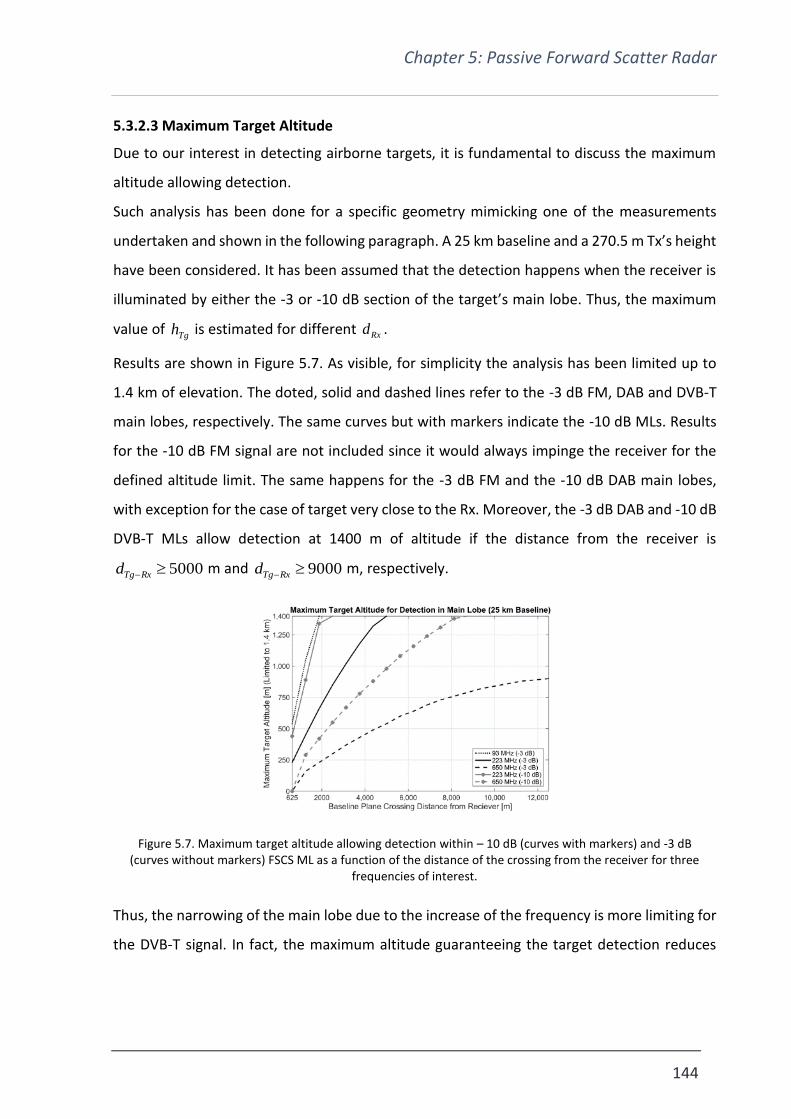
Chapter 5: Passive Forward Scatter Radar
144
5.3.2.3 Maximum Target Altitude
Due to our interest in detecting airborne targets, it is fundamental to discuss the maximum
altitude allowing detection.
Such analysis has been done for a specific geometry mimicking one of the measurements
undertaken and shown in the following paragraph. A 25 km baseline and a 270.5 m Tx’s height
have been considered. It has been assumed that the detection happens when the receiver is
illuminated by either the -3 or -10 dB section of the target’s main lobe. Thus, the maximum
value of Tgh is estimated for different Rxd .
Results are shown in Figure 5.7. As visible, for simplicity the analysis has been limited up to
1.4 km of elevation. The doted, solid and dashed lines refer to the -3 dB FM, DAB and DVB-T
main lobes, respectively. The same curves but with markers indicate the -10 dB MLs. Results
for the -10 dB FM signal are not included since it would always impinge the receiver for the
defined altitude limit. The same happens for the -3 dB FM and the -10 dB DAB main lobes,
with exception for the case of target very close to the Rx. Moreover, the -3 dB DAB and -10 dB
DVB-T MLs allow detection at 1400 m of altitude if the distance from the receiver is
5000RxTgd m and 9000RxTgd m, respectively.
Figure 5.7. Maximum target altitude allowing detection within – 10 dB (curves with markers) and -3 dB (curves without markers) FSCS ML as a function of the distance of the crossing from the receiver for three
frequencies of interest.
Thus, the narrowing of the main lobe due to the increase of the frequency is more limiting for
the DVB-T signal. In fact, the maximum altitude guaranteeing the target detection reduces

Chapter 5: Passive Forward Scatter Radar
145
significantly. For example, the -3 dB ML width allows target detection up to an elevation of
900 m if the target crosses in the middle of the baseline.
Such analysis shows how the use of a specific frequency depends on the system application.
For short baselines, the possibility to detect very high crossing targets is achieved mainly using
low frequencies. On the other hand, for longer baselines higher frequencies could offer some
advantages because of the higher FSCS, which guarantees longer coverage, and because
despite being narrow, due to the longer baseline, the main lobe could still illuminate the
receiver.
5.4 Experimental Measurements with Airliners
System Set Up
Several experimental campaigns have been undertaken in order to test the capabilities of the
processing previously described.
The Sutton Coldfield [14] transmitter was chosen as Tx node for the measurements. Such
broadcast station was chosen because of the high power and the varieties of frequencies
transmitted. Details about the transmitted frequencies are presented in Table 5.3.
Table 5.3. Signals transmitted by Sutton Coldfield transmitter and used during the experiments.
Signal Frequencies [MHz] Signal Bandwidth [MHz] Transmitted Power [kW]
FM
88.3
90.5
92.7
95.6
96.4
97.9
0.150
250
250
250
11
10
250
DAB 222.06
225.65 1.536
8.7
10
DVB-T 650
674 8
200
200

Chapter 5: Passive Forward Scatter Radar
146
The height of the Sutton Coldfield Tx is 270 m above the ground (440 above sea level).
A National Instrument USRP-2950R [15] was used as receiver node. It is a software defined
radio comprising of two full duplex transceivers. Details about the receiving system are
proposed in Appendix E. Table 5.4 summarizes the Rx’s parameters.
For the measurement described in this section only FM and DVB-T signals were used.
Having two channels, the USRP allows the record of a couple of signals simultaneously. Thus,
a combination of DVB-T and FM or DVB-T and DVB-T were recorder. However, as main device
limitation, the two channels share the same sampling rate, which is therefore imposed by the
signal having larger bandwidth. In the specific, the DVB-T signal, with its 8 MHz bandwidth.
Table 5.4. USRP parameters used during the experiments.
However, in the attempt of achieving better performance, the USRP channels bandwidth was
set a bit wider than the needed, 10 MHz. Moreover, the central frequency of each channel
Tunable frequency range 50 MHz-2.2 GHz.
Antennas
DVB-T – Yagi, gain – 8 dBi
DAB – three element DAB
commercial antenna
gain – 6.2 dBi
FM – Yagi FM antenna
Gain – 5dBi
Number of channels 2
USRP channel bandwidth 10 MHz
Azimuth coverage
DVB-T – 20˚,
DAB – 60°
FM – 110˚
Elevation coverage
DVB-T – 20˚
DAB – 60°
FM –70˚
Consumed power 90VA
Chapter 5: Passive Forward Scatter Radar
147
was adjusted to record the biggest number of possible broadcasting channels. Due to the set
parameters, all the six FM signals listed in Table 5.3 were acquired at the same time.
In the experiments, the receiver position was chosen to obtain:
• far-field operations for all different bands. This is possible when both the Tx-target
and target-Rx distances are bigger than the Fresnel length 42DS ;
• operation in optical scattering conditions ( 1D ). This determines an increase of
the forward scatter cross section [8].
Table 5.5. Estimation of far field conditions, electrical dimension and FS main lobe at FM and DVB-T frequencies.
Signal Far field condition S
[m]
Target
Electrical
Dimension
Forward scatter main
lobe
FS ML [Deg]
FM
[90 MHz] 86.7 10.2 h , v)= (5.6;16.3)
DVB-T
[650 MHz] 626.2 73.7 h , v)=(0.8;2.3)
Far field condition, target electrical dimension and FS main lobe for both frequencies used in
the experiment are shown in Table 5.5. The first value has been calculated in a conservative
way for 34D m, the greatest dimension of the biggest detected plane. Results show how
the higher is the frequency and the higher is the Fresnel parameter. For instance, for the DVB-
T signal the target is required to cross at least 626.2 m from the receiver.
Moreover, it can be easily noticed how the optical scattering conditions are hardly satisfied
by FM channels, especially for small targets. In the specific case, the operation happens close
to the Mie zone. This, despite not guarantying the maximum increase of RCS in the forward
direction, does not compromise the detection.

Chapter 5: Passive Forward Scatter Radar
148
(a) (b)
Figure 5.8. Experimental geometry (a) and receiver side in Rx1 (b) with FM and DVB-T antennas.
The first experimental campaign here presented was conducted in the area around the
Birmingham International Airport (BHX) and its main goal was to detect landing and taking off
airplanes. As shown in Figure 5.8, the receiver was placed in two different positions, Rx1
(shown in Figure 5.8 (b)) and Rx2. The former provided a 6 km distance from the crossing
point, the latter a distance of 15 km. Being the distance between Tx and airport around 20 km,
two baselines of 26 and 35 km were tested.
With the use of Flightradar24 [24], it has been possible to collect information about airplanes
track, speed and above sea level altitude. Due to the specific geometry and to the fact landing
and taking off trajectories are similar for all planes (cyan line in Figure 5.8 (a)), targets crossed
the baseline with an angle of approximately 15˚.
Experimental Results
The measurement’s goal was to determine the capability of a passive FSR system in detecting
targets and extracting motion parameters.
The collected data has been processed using the processing shown in Figure 5.1. For the FM
signal, the cut off frequency of the BPF and LPF were 150 kHz and 100 Hz, respectively. On the
other hand, DVB-T signal was processed using an 8 MHz bandwidth BPF and a 100 Hz LPF. In
both cases, the decimation block was set to a 200 Hz sampling rate.
Figure 5.9 shows Doppler signatures and spectrograms for the scenario with receiver at the
position Rx1, determining a 26 km baseline. In this case, the target was taking off from
Birmingham airport. Results refer to the crossing of an Airbus A320, whose dimensions (length

Chapter 5: Passive Forward Scatter Radar
149
x height x wingspan) are (33.8 x 11.7 x 34.1) m. The plane crossed at an altitude of 180 m with
a speed around 240-285 km/h according to Flightradar24.
(a) (b)
(c) (d)
Figure 5.9. Results for an Airbus 320 taking off. Doppler signature and its spectrogram for FM, (a) and (c), and DVB-T (b) and (d), signals. Baseline is 25 km.
The set system parameters allowed the extraction of all FM channels listed in Table 5.3. These
signals present very similar structures. Thus, in order to preserve the clearness of the
presentation, Figure 5.9 (a) shows only two of them. From the figure it can be clearly noticed
how the oscillation rate increases due to the acceleration applied in the taking off. Moreover,
FM signals at 95.6 and 97.9 MHz offer comparable good results despite the 14 dB transmitted
power discrepancy (see Table 5.3). This is a proof of the system robustness to different SNR
values.
5 10 15 20 25 30 35 40-2
-1.5
-1
-0.5
0
0.5
1
1.5
2x 10
-3
Time [s]
Am
plit
ude [
V]
FM Doppler Signatures
FM 95.6 MHz
FM 97.9 MHz
Chapter 5: Passive Forward Scatter Radar
150
A comparison between FM and DVB-T results is proposed in Figure 5.9 (b). The signatures
show similar trends, with the crossing points coinciding at 20 s. It is also visible that the
Doppler frequencies of the FM channels are lower than the DVB-T ones, by a factor equal to
the carrier frequencies ratio. A similar behaviour can be seen in the spectrograms in Figure
5.9 (c) and (d). In fact, it is possible to see how the maximum DVB-T Doppler frequency is
around 6 times bigger than the FM one. In order to allow a better visual comparison between
them, spectrograms have been normalized to the maximum of the DVB-T one.
Another thing that can be noticed from these results is the connection between Doppler and
speed. In fact, a small initial target’s speed corresponds to a small Doppler. Moreover, looking
at the spectrograms, it can be clearly seen how the highest returns are from the FSCS main
lobes. Focussing on the colour scales of the spectrograms a 10 dB difference in the maximum
values can be noticed.
A second measurement with a 35 km baseline (receiver at position Rx2 of Figure 5.8 (a)) has
been undertaken. Due to a condition of opposite wind, planes were landing. Again, a
combination of FM – DVB-T and DVB-T – DVB-T were recorded using the two separate USRP’s
channels. Results are shown in Figure 5.10.
Due to the increased baseline, the Doppler frequency varies in a slower way and the
observation time increases. Such effects, easily spotted in the results, could introduce some
issues. In fact, taking in consideration the FM signal, a longer record is needed to see the
Doppler frequency reaching 1 Hz. This could definitely challenge the detection in case of
strong clutter.
Figure 5.10 (a) proposes results at 650 and 674 MHz for a Bombardier Dash8 Q-400. Target’s
length, height and wingspan are (32.8 x 8.3 x 28.4) m, respectively. The crossing happened at
236 m of altitude with a plane’s speed of 263 km/h, according to Flightradar24. Despite a
phase shift due to the use of two different Rx antennas, the two DVB-T signatures present
similar trends. The deceleration of the airplane due to the landing procedure is well visible in
the spectrogram in Figure 5.10 (b).

Chapter 5: Passive Forward Scatter Radar
151
(a) (b)
Figure 5.10. DVB-T results for a Bombardier Dash8 Q-400 landing. Doppler signature (a) and its spectrogram (b). The baseline is 35 km.
5.5 Experimental Measurements with Light and Ultralight Aircrafts
UoB Scenario and Results
After the good results obtained with airliners, the capabilities of the passive FSR system have
been challenged trying to detect smaller targets. Therefore, new measurements have been
undertaken using a Cessna 172 light aircraft, Figure 5.11 (b), as controlled target. Length,
height and wingspan of this plane are 7.3, 2.3 and 11 m, respectively.
Figure 5.11 (a) shows the experimental scenario. The receiver (85 m above sea level) was
positioned 25 km far from Sutton Coldfield, in an open field near Sibson, a village in the
Leicester area, UK. In addition to FM and DVB-T channels, during this measurement DAB
signals were recorded too. Thus, a three elements DAB antenna was used. The antenna has a
6.2 dBi gain and a 60˚ -3 dB beamwidth in both vertical and horizontal planes.
Two main requirements had to be address in the choice of the measurement location and
scenario:
• to have low altitude flights (the minimum limit for a rural area is 450 m);
• to bypass air traffic limitation in the area of the Birmingham airport.
10 20 30 40 50 60 70-2
-1
0
1
2x 10
-4
Time [s]
Am
plit
ude [V
]DVBT Doppler Signatures
650 MHz
674 MHz

Chapter 5: Passive Forward Scatter Radar
152
Table 5.6. Cessna far field conditions, electrical dimension and FS main lobe at FM, DAB and DVB-T frequencies.
Signal
Far field
condition
S [m]
Target
Electrical
Dimension
Forward scatter
main lobe FS ML
[deg]
FM
[90 MHz] 9.1 3.3 h , v)=(17.4,83.0)
DAB
[225 MHz] 22.7 8.3 h , v)=(6.9,33.2)
DVB-T
[650 MHz] 65.5 23.8 h , v)=(2.4,11.5)
The controlled target trajectories are visible in Figure 5.11 (a). They were decided together
with the pilot, with the aim of having several perpendicular crossings at different altitudes and
in totally safe conditions. Three different crossing heights are here presented: around 450,
800 and 1000 m.
The use of GPS, whose information are shown in Table 5.7 for three different data set, allowed
tracking, data truth and synchronization of the recorded data with the target position.
The receiving bandwidth set to record the data allowed the acquisition of both DAB channels
(222.0 and 225.65 MHz). Thus, as for the FM signal, they have been divided and each of them
processed individually. A 750 MHz BPF and 100 Hz LPF were used to extract the target
signature from the digital audio broadcasting signals.
(a) (b)

Chapter 5: Passive Forward Scatter Radar
153
(c) (d)
Figure 5.11. Experimental FSR scenario (a) with a Cessna 172 (b) used as a target. Rx side (c) with DAB and DVB-T antennas and USRP connected to the laptop (d).
Table 5.7. GPS ground truth for the three records having the Cessna 172 as cooperative target.
Data Crossing distance
from Rx[km]
Crossing Angle
[deg]
Crossing Height a.s.l. (and
above baseline) [m]
Recorded
Signals
D1 9.1 86 483 (354) DVB-T + DAB
D2 9.0 87 788 (659) DVB-T + FM
D3 7.9 85 947 (833) DVB-T + FM
Figure 5.12 (a) and (b) show the results of D1, which is the first acquisition proposed in Table
5.7, for DVB-T and DAB, respectively. The approaching, crossing and leaving the baseline
phases are evident. Despite the transmitted power for a DAB signal is 14 dB lower than the
DVB-T one, detection is perfectly achievable.
(a) (b)
0 5 10 15 20 25 30 35 40-1.5
-1
-0.5
0
0.5
1
1.5x 10
-4
Time [s]
Am
plit
ude [
V]
DVBT Doppler Signature: 650MHz channel

Chapter 5: Passive Forward Scatter Radar
154
(c)
Figure 5.12. Cessna crossing 354 m above the baseline in D1. DVB-T and DAB results.
Comparing Figure 5.12 (a) and Figure 5.9 (a) it is possible to notice the differences in received
power between the crossing of a light aircraft and an airliner.
The DAB spectrogram referring to the D1 data set is visible in Figure 5.12 (c). As explained in
Chapter 3, due to the target crossing the baseline orthogonally and with a constant speed, its
trend results symmetrical.
(a) (b)
0 10 20 30 40 50-5
-4
-3
-2
-1
0
1
2
3
4
5x 10
-4
Time [s]
Am
plit
ude [
V]
DVBT Doppler Signature: 650MHz channel
0.8 10.8 20.8 30.8 40.8 50.8 59.9975-5
-4
-3
-2
-1
0
1
2
3
4
5x 10
-4
Time [s]
Am
plit
ude [
V]
FM Doppler Signature: 97.9MHz channel

Chapter 5: Passive Forward Scatter Radar
155
(c) (d)
(e) (f)
(g) (h)
Figure 5.13. DVB-T and FM Doppler signatures and their spectrograms for D2 (target crossing at 659 m above the baseline) (a)-(d) and D3 data (target crossing 833 m above the baseline) (e)-(h).
0 10 20 30 40 50 60-2.5
-2
-1.5
-1
-0.5
0
0.5
1
1.5
2
2.5x 10
-4
Time [s]
Am
plit
ude [
V]
DVBT Doppler Signature: 650MHz channel
0.7 10.7 20.7 30.7 40.7 50.7 60-2.5
-2
-1.5
-1
-0.5
0
0.5
1
1.5
2
2.5x 10
-5
Time [s]
Am
plit
ude [
V]
FM Doppler Signature: 96.4MHz channel

Chapter 5: Passive Forward Scatter Radar
156
Figure 5.13 shows DVB-T and FM Doppler signatures and spectrograms for the crossings at D2
and D3. A more complete analysis of the effects of the elevation crossing on the system
performance can be done comparing Figure 5.12 and Figure 5.13.
It is interesting to underline how increasing the target’s altitude DVB-T offers poorer
performance. In fact, the spectrogram in Figure 5.13 (c) ( 659Tgh m) shows clearly the
presence of a target. On the other hand, in Figure 5.13 (g) ( 833Tgh m) the Cessna V-shape
is barely visible. In fact, in D3, since the Cessna altitude is almost 1000 m, the receiver is not
illuminated by the FSML. Therefore, a reduction in power is experienced.
In D2 (Figure 5.13 (c) and (d)) and D3 (Figure 5.13 (g) and (h)) DVB-T and FM spectrogram’s
power is comparable. This is connected to the DVB-T and FM FSCS patterns and the fact that,
despite having a lower peak value, the FM ML is wider than the DVB-T one.
Despite the decreased received power due to the higher altitudes, spectrograms in Figure 13
(g) and (h) show the presence of a target crossing.
5.6 Speed Estimation
As a conclusion of this feasibility study on passive forward scatter radar, we tried to estimate
the speed of the detected targets.
The processing working on the spectrogram of the Doppler signature described in Chapter 3
has been used for speed estimation in two different scenarios:
• airliner crossing, at both DVB-T frequencies;
• Cessna crossing, at DAB and DVB-T frequencies.
The estimated values of speed have been then compared with the ground truth ones, either
obtained through Flightradar24, in case of the airliner, or using GPS data, for the light Cessna.
Real and estimated speed values are shown in Table 5.8. As visible, results from the processing
well match the ground truth values.
Table 5.8. Target speed. Estimation Vs. ground truth.
DATA SIGNALS FREQUENCY
MHz
ESTIMATED SPEED
km/h
GROUND TRUTH
km/h

Chapter 5: Passive Forward Scatter Radar
157
4 DVB-T 650 248.4 263
by Flightradar24 DVB-T 674 216.0
D2 DAB
222 176.4 167
by GPS 225 176
DVB-T 650 188.1
5.7 Passive FSR with Moving Receiver
Once proved the capabilities of our FSR device and processing, it has been decided to test the
moving nodes configuration.
As for the previous two chapters, the interest has focused on understanding the system
performance in case of at least one FSR node able to move. Thus, in the following section two
different measurements are introduced: the first one in a low cluttered environment and the
second one in a highly cluttered scenario.
FHR Scenario and Results
This section is focused on the description of another measurement undertaken in
Eckernförde, Germany, in the Bundeswehr Technical Centre for Ships and Naval Weapons by
the FHR group, Figure 5.14 (a). For the measurement, the FHR PARASOL, a passive radar
device, was used. It was installed on the moving AM8 boat shown in Figure 5.14 (c).
The features of such receiver are summarized in Table 5.9. The PARASOL has been developed
to operate in passive mode using DVB-T signals. It uses log-periodic antennas and has two
receiving channels formed by a RF block followed by an ADC/FPGA block. The local oscillators
are controlled by GPS. Acquisition and processing are achieved through a PC connected to the
system.
Table 5.9 . PARASOL parameters.
PARASOL SYSTEM
Band 470-780 MHz
Number of antennas 2
Chapter 5: Passive Forward Scatter Radar
158
The Kiel Tx, whose information are contained in Table 5.10 has been used as transmitter of
opportunity.
Figure 5.14 (b) shows the cooperative target chosen for the measurement, an ultralight
Delphin whose dimensions are 6.5 x 2.2 x 9.4 m, length, height and wingspan, respectively.
While testing bistatic operations, the aircraft, Tx and Rx occurred to be in a typical FSR
scenario, with bistatic angle nearly equal to 180˚ (Figure 5.14 (a) with target trajectory
indicated by the cyan line).
The use of a Spatial Dual Inertial Measurement Unit (IMU), placed nearby the antennas
allowed to track the receiver motion.
Table 5.10. Kiel transmitter parameters.
Signal DVB-T
Frequency 666 MHz
Modulation 16 QAM
Site Elevation 38 m
Antenna Height 219 m
ERP (kW) 43
Polarization H
Antenna one vertically and one horizontally polarized log-periodic
antennas
Number of channels 2
Bandwidth channel 7.61 MHz
Azimuth coverage 60°
Elevation coverage 60°
Real-time processing Yes
Consumed power 500 VA

Chapter 5: Passive Forward Scatter Radar
159
(a) (b)
(c)
Figure 5.14. FHR experimental scenario (a). The ultralight Delphin used as a target (b) and the AM8, platform where the receiver was installed (c).
As for the previously presented records, the processing in Figure 5.1 has been used on the FHR
data. Figure 5.15 shows the two extracted Doppler signatures (one acquired by the vertically
(V) and one by the horizontally (H) polarized channel) and their spectrograms.
(a)

Chapter 5: Passive Forward Scatter Radar
160
(b) (c)
Figure 5.15. FHR experimental results. Doppler signatures (a) and spectrograms for the horizontally (b) and vertically (c) polarized acquisitions.
These results confirm that the transmitted and scattered signal have the same polarization. In
fact, the spectrogram of the horizontally polarized channel, Figure 5.15 (b) presents a bright
spot around 27 s, when the crossing happens. This is due to the peak of FSCS. On the other
hand, the spectrogram from the vertically polarized channel, Figure 5.15 (c), does not present
such bright spot. In addition to that, it can be also noticed that when the strong forward
scatter effect vanishes both H and V channels’ spectrograms show the presence of a target. A
motivation to such effect could be that the spectrogram’s “wings” refer to a bistatic scattering,
rather than a FSR one.
Highly cluttered environment
In this section, two different measurements with passive forward scatter radar with moving
receiver in a highly cluttered environment are presented.
Sutton Coldfield has been kept as transmitter of opportunity and the Rx, our USRP-2950R, has
been mounted on our test car, with DAB and DVB-T antennas on dedicated musts placed on
the vehicle’s roof Figure 5.16. IMU system set next to the antennas was used for ground truth.
The measurements geometries are shown in Figure 5.17. In (a) and (b) the scenarios in case
of receiver moving along and perpendicularly to the baselines are proposed. In both
screenshots the LoS between Tx and Rx is visible (yellow solid line) as well as the plane landing
trajectory (blue line) and the receiver’s track (pink line).

Chapter 5: Passive Forward Scatter Radar
161
Figure 5.16. Receiver side. Rx has been installed on our laboratory car. DAB and DVB-T antennas are visible mounted of the roof of the vehicle.
Receiver trajectories have been chosen to guarantee:
• long path and therefore a pretty constant speed;
• safe drive at moderate speed;
• crossing of landing airplanes;
• nearly along the baseline and orthogonal to the baseline trajectories.

Chapter 5: Passive Forward Scatter Radar
162
(a)
(b)
Figure 5.17. Experimental scenarios with receiver moving along the baseline (a) and perpendicularly to it (b).
In the first measurement, Figure 5.17 (a), due to the receiver motion the baseline varies
between 24.2 and 24.8 km, with the Rx moving approximately 620 m. The distance between
the crossing point and the receiver is between 4.5 and 5.5 km. The car with the USRP on board
moved 20 mph (nearly 9 m/s) trying to keep the speed as constant as possible.
In order to catch the crossing while moving, we started driving the car whenever a plane was
approaching. Records started as soon as the cruise speed was reached and ended once
reached the other side of the path, lasting approximately 70 s.
A stationary result at 650 MHz is shown in Figure 5.18. The presence of a target crossing the
baseline is clearly evident in both time (a) and frequency (b) domain. However, due to the
specific trajectory and location, only the target’s approaching phase is visible, as can be
noticed from the single wing of the spectrogram in Figure 5.18 (b).

Chapter 5: Passive Forward Scatter Radar
163
(a) (b)
Figure 5.18. Stationary results for the shortest baseline in Figure 5.17 (a). DVB-T Doppler signature (a) and its spectrogram (b).
Doppler signature and its normalized spectrogram in the case of receiver moving are
presented for DVB-T, Figure 5.19 (a) and (b), and DAB, Figure 5.19 (c) and (d). Due to Rx
motion, Doppler shift and clutter Doppler spread deteriorate the acquired signal. The level of
disturbance is stronger than the target’s return and compromises the detection. In fact,
comparing the Doppler signatures in Figure 5.18 (a) and Figure 5.19 (a), it is evident how the
return from the target in the stationary case is much smaller than the one measured in case
of receiver moving.
(a) (b)
40 45 50 55 60 65 70 75 80-2
-1.5
-1
-0.5
0
0.5
1
1.5
2x 10
-3
Time, s
Am
plitu
de
, V
0 10 20 30 40 50 60 70-0.02
0
0.02
0.04
0.06
0.08
0.1
Time, s
Am
plitu
de
, V

Chapter 5: Passive Forward Scatter Radar
164
(c) (d)
Figure 5.19. Results for the receiver moving as in Figure 5.17 (a). Doppler signature and spectrogram at 650 MHz, (a) and (b), and 222.06 MHz, (c) and (d).
The bright returns in the spectrograms result very well defined and contained around 40 Hz
for DVB-T and 16 Hz for DAB. Such “edge” is due to the Doppler shift introduced by the receiver
motion. The increasing and decreasing trend follows the car’s speed variation. The contributes
below the Doppler shift border are due to the presence of the vegetation along the path.
The second scenario we investigated, Figure 5.17 (b), considers the receiver moving
perpendicularly to the baseline. The LoS is between 24.5 and 24.7 km and the distance Rx-
crossing point is around 4.5/5.5 km. In this configuration, the receiver moved with two
different speeds, 15 and 30 mph (around 6.7 and 13.4 m/s), for approximately 350 m.
Figure 5.20 (a) and (c) show the Doppler signatures for both speed motions at 650 MHz in case
of plane crossing. Their spectrograms are presented in Figure 5.20 (c) and (d). Similarly to the
previous measurement, returns from the environment are stronger than the ones from the
targets, which are therefore not detectable. Due to the different concentration of vegetation
along the Rx path, spectrograms show areas with high and low Doppler frequency returns.
0 10 20 30 40 50 60 70-0.02
0
0.02
0.04
0.06
0.08
0.1
Time, s
Am
plitu
de
, V

Chapter 5: Passive Forward Scatter Radar
165
(a) (b)
(c) (d)
Figure 5.20. Results for the receiver moving as in Figure 5.17 (b). DVB-T Doppler signature and spectrogram
for 15Rxv mph, (a) and (b), and 30Rxv mph, (c) and (d).
The IMU data gave us full knowledge of Rx speed and direction, instant by instant. Thus, it has
been possible to link the receiver motion to the wide environmental spectral components
shown in the spectrograms.
Doppler shift and clutter Doppler spread effects on the received signature can be observed in
Figure 5.21. (a) and (b) show the power spectral densities for the DAB signal when the receiver
moves along the baseline or perpendicular to it, respectively. As stated in Chapter 4, the PSDs
does not present an evident peak indicating the Doppler shift, despite clearly showing
presence of clutter. However, it can be seen the environmental return is below the value
0 10 20 30 40-0.02
-0.01
0
0.01
0.02
0.03
0.04
0.05
0.06
0.07
Time, s
Am
plitu
de
, V
0 5 10 15 20-0.02
-0.01
0
0.01
0.02
0.03
0.04
0.05
0.06
0.07
Time, s
Am
plitu
de
, V

Chapter 5: Passive Forward Scatter Radar
166
Tg
DS
vf 2 ( 5.7 )
The upper limit of the Doppler shift, calculated according to ( 5.7 ) using the IMU data, has
been overlapped to the spectrograms of the results. Figure 5.21 shows such comparison for
DAB when the receiver moved along the baseline (c) and perpendicular to it (d). As visible
from the picture, the trend calculated using ( 5.7 ) (in black solid line) describes very well the
edge of the spectrogram’s brightest returns. Thus, it can be deducted that, in case of moving
node and presence of dense clutter, the combination of Doppler shift and clutter Doppler
spread will fill the area below the value obtained with ( 5.7 ). Thus, detection would be possible
whenever at least part of the target return is higher than the Doppler shift.
(a) (b)
(c) (d)
Figure 5.21. DAB PSDs and spectrograms with Doppler shift calculated using the IMU data (black line) for Rx moving along the baseline, (a) and (c), and perpendicular to it, (b) and (d).

Chapter 5: Passive Forward Scatter Radar
167
5.8 Conclusions
In this chapter, the concept of passive forward scatter radar has been introduced. The
simplicity of FSR combines very well with the use of transmitters of opportunities. In fact, as
long as the receiver pointing at the chosen transmitter can detect its signal an FSR link is built.
An initial study on the possibility to develop multi-frequencies passive configuration has been
undertaken in the first part of the chapter. Since dealing with transmitters of opportunities, it
has been necessary to understand the power limitations and the maximum range available for
detection. These calculations have been done according to the idea of experiment we had in
mind. In fact, the power budget is strongly dependent on the selected transmitter (its
transmitted power and frequency) and the targets aimed to be detected.
Being our goal the detection of airplanes, we focused also on the study of the maximum
crossing elevation allowing to see a target.
After these preliminary investigations, some experimental results have been presented. In the
attempt to challenge our system and test the capabilities of a FSR device, different targets
have been considered. Initially, experiments with airliners have been undertaken. Despite the
unfavourable targets’ trajectories, characterized by a very small crossing angles, detection has
been possible. Thus, the system capabilities have been challenged using a smaller vehicle, a
light Cessna aircraft, moving with various trajectories. The controlled target crossed the area
between Tx and Rx several times at different altitudes. This has allowed the comparison of
returns at different frequencies. In fact, both forward scatter cross section and main lobe
depend on the wavelength. Therefore, according to the scenario and the applications, one
frequency could be better than another one. In general, the use of a multi-frequency system,
feasible in case of passive FSR due to its simplicity, would be suggested. Results from another
FSR experiment have underlined the effects of different antennas’ polarizations on the target
detection.
To verify the capabilities of a passive stationary FSR geometry, a moving receiver configuration
has been tested. In fact, as explained already in the previous chapters, a moving nodes FSR
would introduce several advantages and overcome some of the typical FSR limitations. The
experiment’s aim has been to investigate the effect of receiver motion on the system

Chapter 5: Passive Forward Scatter Radar
168
performance. As expected, results have shown presence of Doppler shift, introduced by the
motion of the receiver. In addition to that, the presence of a significant amount of vegetation
surrounding the experimental area has determined clutter Doppler spread. Such strong
contributes due to the motion of the receiver combined with the weak return from the target
have inhibited the airplane detection. However, results have shown that the clutter Doppler
spread is limited by the Doppler shift. Therefore, a target could be detected whenever its
crossing determines contributes higher than the Doppler shift values.
To summarize then, this chapter has focused on the concept of passive FSR, at several
frequencies and at both stationary and moving configuration. Results have shown good target
detection and speed estimation capabilities for the stationary case. However, whenever
considering a moving Tx/Rx FSR configuration, the presence of Doppler shift and clutter
Doppler spread can challenge the system.

Chapter 5: Passive Forward Scatter Radar
169
5.9 Bibliography
[1] M. Marra, A. D. Luca, S. Hristov, L. Daniel, M. Gashinova, and M. Cherniakov, ‘New algorithm for signal detection in passive FSR’, in 2015 IEEE Radar Conference, 2015, pp. 218–223.
[2] M. Contu et al., ‘Passive Multifrequency Forward-Scatter Radar Measurements of Airborne Targets Using Broadcasting Signals’, IEEE Transactions on Aerospace and Electronic Systems, vol. 53, no. 3, pp. 1067–1087, Jun. 2017.
[3] S. S. Haykin, Communication systems, 4th ed. New York: Wiley, 2001.
[4] European Telecommunications Standards Institute, ‘ETSI TS 563, Digital Audio Broadcasting (DAB); Transport of advanced Audio Coding (AAC) audio’, Jan. 09.
[5] European Telecommunications Standards Institute, ‘ETSI EN 300 744, Digital Video Broadcasting (DVB); framing structure, channel coding and modulation for digital terrestrial television’, Jan. 09.
[6] D. E. Hack, L. K. Patton, B. Himed, and M. A. Saville, ‘Detection in Passive MIMO Radar Networks’, IEEE Transactions on Signal Processing, vol. 62, no. 11, pp. 2999–3012, Jun. 2014.
[7] C. Hu, V. Sizov, M. Antoniou, M. Gashinova, and M. Cherniakov, ‘Optimal Signal Processing in Ground-Based Forward Scatter Micro Radars’, IEEE Transactions on Aerospace and Electronic Systems, vol. 48, no. 4, pp. 3006–3026, Oct. 2012.
[8] M. Gashinova, L. Daniel, V. Sizov, E. Hoare, and M. Cherniakov, ‘Phenomenology of Doppler forward scatter radar for surface targets observation’, Sonar Navigation IET Radar, vol. 7, no. 4, pp. 422–432, Apr. 2013.
[9] M. Gashinova et al., ‘Signal characterisation and processing in the forward scatter mode of bistatic passive coherent location systems’, EURASIP Journal on Advances in Signal Processing, 2013.
[10] N. E. A. Rashid, M. Antoniou, P. Jancovic, V. Sizov, R. Abdullah, and M. Cherniakov, ‘Automatic target classification in a low frequency FSR network’, in 2008 European Radar Conference, 2008, pp. 68–71.
[11] S. Hristov, L. Daniel, E. Hoare, M. Cherniakov, and M. Gashinova, ‘Target Shadow Profile Reconstruction in ground-based forward scatter radar’, in 2015 IEEE Radar Conference (RadarCon), 2015, pp. 0846–0851.
[12] ‘CST Microwave studio’ [Online]. Available: https://www.cst.com/Products/CSTMWS. .
[13] V. Sizov, M. Cherniakov, and M. Antoniou, ‘Forward scattering radar power budget analysis for ground targets’, Sonar Navigation IET Radar, vol. 1, no. 6, pp. 437–446, Dec. 2007.

Chapter 5: Passive Forward Scatter Radar
170
[14] ‘Sutton Coldfield (Birmingham, England) Full Freeview transmitter’, UK Free TV. [Online]. Available: https://ukfree.tv/transmitters/tv/Sutton_Coldfield/PGSTART2590/. [Accessed: 15-Oct-2017].
[15] ‘Overview of the NI USRP RIO Software Defined Radio - National Instruments’. [Online]. Available: http://www.ni.com/white-paper/52119/en/. [Accessed: 15-Oct-2017].
[16] ‘Satellite Coverage | Our Satellites’, Inmarsat. [Online]. Available: https://www.inmarsat.com/about-us/our-satellites/our-coverage/. [Accessed: 18-Oct-2017].
[17] M. Gashinova, L. Daniel, S. Hristov, X. Lyu, A. G. Stove, and M. Cherniakov, ‘Design and Validation of a Passive Radar Concept for Ship Detection using Communication Satellite Signals’, IEEE Transactions on Aerospace and Electronic Systems, vol. PP, no. 99, pp. 1–1, 2017.

Chapter 6: MIMO Forward Scatter Radar
171
MIMO Forward Scatter Radar
Glossary of Abbreviations
AWG Arbitrary Waveform Generator
DPO Digital Phosphor Oscillator
FSR Forward Scatter Radar
MIMO Multiple Input Multiple Output
MISO Multiple Input Single Output
PRF Pulse Repetition Frequency
PRT Pulse Repetition Time
Rx Receiver
SCR Signal to Clutter Ratio
SISO Single Input Single Output
SNR Signal to Noise Ratio
Tx Transmitter
6.1 Introduction
Multiple Input Multiple Output (MIMO) is a concept based on the use of several antennas at
both transmitter (Tx) and receiver (Rx) side. Such configuration, already briefly discussed in
Chapter 1, offers a performance improvement whenever the information acquired is properly
processed together. Bigger area coverage, increased performance in target detection and
power benefits are just few of these advantages [1]. On the other hand, due to the more
complex structure, some drawbacks are introduced as well. In fact, the cost of the whole
system could be higher and the processing of bigger amount of data more difficult [1].

Chapter 6: MIMO Forward Scatter Radar
172
Figure 6.1 Different communication configurations.
Figure 6.1 shows different communication configurations defined by the number of
transmitters and receivers used. From Single Input Single Output (SISO) to MIMO, all the
combinations of single or multiple Txs/Rxs are covered.
The simultaneous use of multiple transmitters and multiple receivers is only possible when all
the different signals can be recognized and separated. Therefore, the key point of such
configuration is the orthogonality between signals. Orthogonal waveforms are characterized
by a very low cross-section, ideally equal to zero, allowing the separation of the different
contributes in the receivers. MIMO systems adopt different methodology to guarantee
orthogonality between signals, achieved by time, frequency, code or polarization diversity.
During the last years, many studies on MIMO radars have been undertaken [2]–[7] to
investigate advantages and disadvantages of this configuration.
Similarly, the development of Multiple Input Single Output (MISO) forward scatter radar (FSR)
configurations [8]–[11] has shown margins of improvement in target detection and motion
parameter estimation even in critical scenarios, such as low signal to clutter ratio (SCR) or
crossing of small and slow objects.
On the base of these past studies, the implementation of a multiple transmitters/ multiple
receivers system should simplify detection and tracking, enabling a more accurate estimation
of target’s speed, crossing point and crossing angle. Moreover, a more precise estimation of

Chapter 6: MIMO Forward Scatter Radar
173
the object motion together with its observation at different view angles would help in target
classification and profile reconstruction.
In this chapter for the first time is described the development of a MIMO FSR. An initial study
on such configuration has been undertaken. In order to test the capabilities of the innovative
geometry, a multiple transmitters multiple receivers FSR system has been set up and tested
in a controlled and scaled scenario.
This chapter is divided in three main parts:
• the first one offers a broad picture of the MIMO system we are aiming to build.
Therefore, the way a FSR could operate in a multi Txs and multi Rxs scenario is shown.
An innovative technique for the estimation of target motion parameters is also
proposed;
• the second part describes the developed system. Details of the equipment, how all the
components are connected together and the specific geometry defined for our
scenario are presented;
• the last part of the chapter focuses on the measurements undertaken. The way to
extract of the Doppler signature in our specific case and some experimental results are
shown. Moreover, the new processing enabling the estimation of the target’s
kinematic parameters is herein tested.
I have been the main responsible for the MIMO FSR development. Thus, I worked on all the
aspects herein discussed. The project here presented has been the base for the publications
of [12]–[14].
6.2 MIMO Geometry
The system geometry is assumed to be formed by two parallel arrays of N transmitters
10 ,..., NTTTxs and K receivers 10 ,..., KRRRxs with Td and Rd the distances
between two adjacent transmitting and receiving nodes, respectively. Such arrays are aligned
orthogonally to the 0T - 0R baseline, whose overall length is equal to D . Figure 6.2 shows the
system’s geometry. 0R is the centre of the coordinates system and all the receiving nodes

Chapter 6: MIMO Forward Scatter Radar
174
(yellow circles) are placed along the x axis. The N transmitters (blue circles) are places in
Ddn T , , with 1,...0 Nn .
Figure 6.2. Geometry of the MIMO forward scatter radar system.
As visible from Figure 6.2, each couple of Tx and Rx forms a baseline knL ,
. As for n ,
1,...0 Kk . The red circle in the picture represents a target, the red line its trajectory.
Given such configuration, it is possible to calculate the length of all the baselines. Neglecting
the target height, the distance between the generic transmitter nT and receiver kR is
calculated as ( 6.1 ).
22
, TRkn dndkDL ( 6.1 )
Considering a target moving with a constant velocity its position in time is obtained as
following
tvyty
tvxtx
y
x
0
0 ( 6.2 )
with 0x and 0y the coordinates of the target at 0t .
Therefore, it is possible to calculate the instant when the target crosses the kn, baseline as
Dvkdndv
kdndyDkdxt
xRTy
RTRoc
kn
0
, ( 6.3 )
Thus, the crossing point is defined as

Chapter 6: MIMO Forward Scatter Radar
175
Dvkdndv
Dkvknvyvxx
xRTy
xxyoc
kn
0
,
Dvdknv
vyvkdxy
xy
xyoc
kn
0
,
( 6.4 )
Parameters Estimation Based on Multiple Baselines Crossing Times
As already discussed in the previous chapters, the estimation of motion parameters is crucial
for a radar system. In addition to the techniques discussed in Chapter 3, a multiple
transmitters and multiple receivers configuration allows to estimate target motion
parameters based on information regarding the multiple crossings. In fact, assuming the
presence of a target moving with constant speed, the information regarding the crossing
times, described by equation ( 6.3 ), can be jointly used to estimate its motion parameters.
( 6.3 ) can be re-written as
DdkkdndyDxtDvtkdndv RRT
c
knx
c
knRTy 00)( ( 6.5 )
which can be expressed using the following matrix
R
y
x
c
knRT
c
knRT dk
v
v
y
x
tDkdndtDkdnd
0
0
/)(/)(1 ( 6.6 )
The four unknown parameters in ( 6.6 ) are 0x , xv , 0y and yv corresponding to the target
coordinates and velocity components on the x and y axis, respectively. These parameters allow
to define speed, crossing angle and crossing point of a moving object. Given a vector of four
unknown parameters, it is necessary to combine the information of at least four crossings.
For a MIMO configuration exploiting N transmitters and K receivers, the number of baseline
is KNP . Assuming 4P , it is possible to obtain a solution to the equation proposed
[14]. Thus, combining the knowledge regarding the P crossing times, the following linear
system of equations is obtained.

Chapter 6: MIMO Forward Scatter Radar
176
R
P
y
x
knRPTPknRPTP
knRTknRT
knRTknRT
knRTknRT
d
k
k
k
k
v
v
y
x
tDdkdntDdkdn
tDdkdntDdkdn
tDdkdntDdkdn
tDdkdntDdkdn
PPPP
3
2
1
0
0
00
0
33
0
33
0
22
0
22
0
11
0
11
/)(/)(1
/)(/)(1
/)(/)(1
/)(/)(1
3333
2222
1111
( 6.7 )
Defining the matrix C as
00
0
33
0
33
0
22
0
22
0
11
0
11
/)(/)(1
/)(/)(1
/)(/)(1
/)(/)(1
3333
2222
1111
PPPP knRPTPknRPTP
knRTknRT
knRTknRT
knRTknRT
tDdkdntDdkdn
tDdkdntDdkdn
tDdkdntDdkdn
tDdkdntDdkdn
C ( 6.8 )
the target motion parameters can be estimated as follows
R
P
TT
y
x
d
k
k
k
k
v
v
y
x
3
2
1
10
0
CCC ( 6.9 )
6.3 System Development
As done for the topics described in the previous chapters, part of this project has focused on
the identification of system capabilities through experimental campaigns. Therefore, it has
been necessary to build a FSR prototype comprising multiple transmitters and receivers
allowing to undertake measurements in a scaled scenario. This paragraph focuses on the
description of all the steps that brought to the development of such MIMO FSR.
The initial project requirements were to operate in:
• a scaled and controlled scenario offering possibility of repeatable measurements
under safe conditions;
• high signal to noise ratio (SNR);
• far field, using controllable targets.

Chapter 6: MIMO Forward Scatter Radar
177
Therefore, the prototype described in this chapter is the result of compromises in order to
guarantee these listed conditions.
Equipment
6.3.1.1 Transmitter side – Arbitrary Waveform Generator (AWG)
The transmitter side comprises a Tektronix AWG7102 Arbitrary waveform generator, Figure
6.3. Such device allows the creation, generation or replication of signals. It is characterized by:
• up to two output channels;
• sample rate from 5 to 20 GS/s;
• 10 dBm output power Vp- p.
Figure 6.3. Arbitrary waveform generator.
More information about the AWG can be found in [15].
6.3.1.2 Receiver Side – Digital Phosphor Oscillator (DPO)
The receiver side is characterized by the use of a Tektronix DPO 70004, a mixed signal
oscilloscope allowing setup, acquisition and analysis of data signals. Such device is
characterized by:
• up to 4 channels;
• sample rate from 6.25 to 50 GS/s.
Figure 6.4 shows the Tektronix DPO series. More details regarding the DPO 70004 can be
found in [16].

Chapter 6: MIMO Forward Scatter Radar
178
Figure 6.4. Digital phosphor oscilloscopes.
System Design
The AWG and DPO constitute the core of our MIMO FSR system. In fact, the potentialities of
these devices have allowed the development of a 2 transmitters and 4 receivers configuration.
Orthogonality between signals has been provided using different frequencies appropriately
separated. The two transmitters operated at 3.1 and 3.4 GHz.
The schematics of the system are shown in Figure 6.5.
Figure 6.5. Block diagram of the developed MIMO FSR.
Transmitting and receiving blocks are visible on the left and right side of Figure 6.5,
respectively. Due to AWG and DPO’s need to be synchronized, operation is done in pulse
mode. Gaussian shaped pulses having a 10 MHz bandwidth have been transmitted at both 3.1
and 3.4 GHz. Being interested in the extraction of the Doppler signature, the shape of the
pulse itself is not important. The pulse repetition frequency (PRF) has been set considering

Chapter 6: MIMO Forward Scatter Radar
179
project and system objectives. In a radar system, such parameter is limited by two main
specifics: the maximum unambiguous range and target speed. For our specific purpose, since
we aimed to operate in a scaled scenario with a slow moving target, the value of the PRF has
been determined by the following relation
MaxB
Max
R
cPRF
v
_
4
( 6.10 )
For example, assuming to operate with a target moving with a speed Maxv around 2 m/s, and
with a geometry allowing a maximum bistatic distance MaxBR _
of nearly 30 m, the previous
equation would allow having PRF values from almost 100 Hz up to 10 MHz. Therefore,
considering (6.10), the pulse repetition frequency has been set equal to 1 kHz. Such value has
been chosen close to the lower limit in order to avoid memory problems given by a too high
PRF but bigger than 100 Hz to have the possibility to operate with targets moving faster than
2 m/s.
As visible in Figure 6.5, each AWG7102 output channel is connected to a 25 dB amplifier and
transmitted using a directive horn antenna, Figure 6.6 (a). The gain introduced by such
antenna is shown in Figure 6.6 (b) and it is close to 8 dBi for the selected frequencies.
(a) (b)
Figure 6.6. Horn antenna (a) and its features (b).
The combination of amplifier and horn antenna has been introduced to guarantee a high level
of transmitted power.
The receiver side is characterized by the use of omnidirectional antennas made by Dr. Vladimir
Sizov, Figure 6.7 (a). Their dimension can be understood combining the information in Figure

Chapter 6: MIMO Forward Scatter Radar
180
6.7 (b) and Table 6.1. The antenna pattern simulated using CST Microwave Studio [17] is
proposed in Figure 6.7 (c). From the simulation, the gain of the such antennas appears to
around 2 dB at the operational frequencies.
(a)
(b) (c)
Figure 6.7. Omnidirectional antenna (a), its dimensions (b) and its radiation pattern calculated at 3 GHz.
Table 6.1 Omnidirectional antennas features.
Dimensions (mm) Bandwidth (GHz)
D1 D2 (inner) L B VSWR<1.2 VSWR<1.6 Radiation pattern
26 24 (22) 18 2.2 2.4-4.8 2.2-6 2-5
The signal received by the antenna passes through a block formed by a bandpass filter
followed by an amplifier, Figure 6.8 (a).
D1
D2
L
B

Chapter 6: MIMO Forward Scatter Radar
181
(a)
(b)
Figure 6.8. Filter plus amplifier (a) and its characteristic (b).
The properties of such block are shown in Figure 6.8 (b). The band pass filter let pass
frequencies between 3 and 3.5 GHz. The signal is then amplified by 23/25 dB.
Geometry
All the measurements took place on the roof of our university building. This location has
allowed the undertaking several measurements in a controlled scenario, avoiding external
changing and interfering factors. Moreover, in absence of waterproof equipment, such choice
has given the possibility to acquire a good quantity of real data even in unpredictable weather
conditions. On the other hand, due to the limited area available on the roof, and avoiding to
place the antennas close to walls or other obstacles that could have introduced interference
and/or multipath, the experimental geometry has been reduce to an 8 x 10 meters area.

Chapter 6: MIMO Forward Scatter Radar
182
As previously said the equipment used has allowed a 2 transmitters – 4 receivers
configurations. Figure 6.9 shows the geometry used for the measurements.
The selected geometry has been decided as a compromise to obtain long baselines, guarantee
enough power and similar received SNR for all the channels. As already explained previously,
in order to suppress the presence of interfering objects placed on the roof (such as fans or
walls), the first and last receivers have been positioned one meter far from the possible
multipath sources.
Figure 6.9. Multi transmitters - multi receivers FSR geometry.
Figure 6.9 is based on the already explained configuration presented in Figure 6.2. The centre
of the coordinate system is in 1R , which is the first of the four receivers, represented by the
yellow circles. The other three Rxs are placed on the x axis, uniformly positioned along the 8
m available length. Therefore, the distance between each couple of Rxs, Rd , is 2.66 m.
Transmitters, blue circles on the left, are facing the Rx side. Their coordinates are (2,10) and
(6,10) respectively, with Td , the distance between them, equal to 4 meters. Due to the
presence of 2 Txs and 4 Rxs, 8 baselines are available. Their length is proposed in Table 6.2.
Table 6.2. Baselines' length.
11Bl & 24Bl 12Bl & 23Bl 13Bl & 22Bl 14Bl & 21Bl

Chapter 6: MIMO Forward Scatter Radar
183
10.20 m 10.02 m 10.54 m 11.66 m
Targets
As said previously, the aim of this project was to investigate the features of a MIMO FSR
system in a scaled scenario. Therefore, as for the baselines, the target used was required to
be relatively small. A remote control toy car, Figure 6.10 (a), has been selected as cooperative
crossing object. The possibility to control the target has allowed to test different crossing
trajectories. During the experiments, the toy car has been equipped with rectangular
cardboard boxes installed directly over its structure. Such boxes have been built during
previous Microwave Integrated System Laboratory (MISL) projects to create targets having
approximately the RCS of a sheep, Figure 6.10 (b), and a fox, Figure 6.10 (c).
(a)
(b) (c)
Figure 6.10. Remote controlled toy car (a) with rectangular support approximating the RCS of a sheep (b) and a fox (c).
The given geometry and selected targets have been chosen as a compromise to satisfy
scattering in optical region and far field operation. In fact, as described in Chapter 2, the first
condition determines an increase of the target RCS; the second one guarantees the presence

Chapter 6: MIMO Forward Scatter Radar
184
of both leakage and scattered signal, fundamental in FSR [18]. As usually happens for radar
systems, the dimensions of the targets, shown in Table 6.3, are much bigger than the
wavelengths. Thus, scattering in the optical region is achieved. Far field values are also
presented in Table 6.3, together with the radar cross section of each target at both operational
frequencies.
Table 6.3. Targets information.
Dimensions Far Field RCS
@3.1 GHz @3.4 GHz @3.1 GHz @3.4 GHz
Sheep (0.74x0.615)m 11.32 m 12.40 m 24.10
dBsm
24.90
dBsm
Fox (0.60x0.405)m 7.44 m 8.16 m 19.09
dBsm
19.90
dBsm
RCS values have been calculated using the formula (1.2), considering the size of the cardboard
boxes plus the bottom part of the toy car, used as moving base. As visible, the radar cross
section for the big and small target is around 25 and 20 dBsm, respectively.
The far field FF has been calculate using the following formula
22dFF ( 6.11 )
with d the biggest dimension of the target and the wavelength. The comparison between
values proposed in Table 6.3 and length of the baselines in Table 6.2, shows how it is not
possible to operate in the far field. In fact, due to the limited experimental surface, the
distance transmitters-receivers cannot be extended. However, results proposed in the
following pages present the typical chirp-like structure allowing the extraction of target
motion parameters.

Chapter 6: MIMO Forward Scatter Radar
185
6.4 Experimental Results
In this section, some results obtained during our experimental campaigns are shown. System
and geometry used are those described previously. Thus, a 2 by 4 MIMO FSR system has been
tested to define its capabilities in terms of detection and parameters estimation.
The experimental set up is proposed in Figure 6.11. It is possible to see the transmitter side
with the AWG 7022 connected to the two transmitters Tx1 and Tx2, transmitting Gaussian
shaped pulses of 10 MHz bandwidth with a PRF of 1 kHz at carrier frequencies of 3.1 and 3.4
GHz, respectively. Analogously, the DPO 70004 on the receiver side is connected to the four
Rxs, acquiring signals from 3 to 3.5 GHz. The heights of Txs and Rxs is 0.35 and 0.25 m
respectively.
Figure 6.11. Experimental set up.
Extraction of the Doppler Signature
The extraction of the target Doppler signature is conceptually identical to the one presented
in Chapter 2. It is worth to underline that the total length of the signal recorded is nPRFLF
, with FL and n the length of the frame in samples and the number of seconds recorded,
respectively. Each frame is composed by a 400 nsec window sampled at 12.5 GS/s. Thus, its
length is equal to 5000 samples. Due to the big size of the recorded signal, it has been
necessary to process the received files in smaller parts. It has been decided to operate by
frame.

Chapter 6: MIMO Forward Scatter Radar
186
Figure 6.12 shows the digital processing scheme used for this specific configuration. tsR is
the received signal at the input of one of the four receivers. Remembering that the system
operates at 1.31 f GHz and 4.32 f GHz and that the Rxs side has physical band pass filters
from 3.0 to 3.5 GHz, tsR contains both transmitted signals. Thus, an initial BPF is used to
isolate the signal transmitted at either 1f or
2f . Obviously, apart from this first block, the
processing of the two signals is identical and follows the scheme in Figure 6.12. Once
separated the contributes related to the first and second transmitter, operation is done on
single frames. For each of them, the processing is as the typical one described in Chapter 2: a
square law detector followed by a low pass filter. Due to the high sampling rate, LPF1 has been
designed wider than needed, leaving space to a further narrower low pass filter. To reduce
the size of the signal and allow a faster processing, a block taking the maximum value of the
signal at the output of LPF1 is used. In such way, the length of the Doppler signature is cut
down by a factor equal to the length of the frame and the sample rata becomes equal to the
PRF. A second low pass filter LPF2, designed according to the maximum target speed aimed,
is used to further reduce the presence of unwanted contributes.
Figure 6.12. MIMO FSR signal processing.
The output of the second LPF (LPF2) is the final Doppler signature. Figure 6.13 shows the signal
at the beginning of the processing and at the end. In (a) the single-frame signal after the initial
BPF is presented. The target Doppler signal extracted using the processing in Figure 6.12 is
shown in Figure 6.13 (b).

Chapter 6: MIMO Forward Scatter Radar
187
(a) (b)
Figure 6.13. Single-frame signal after the band pass filter (a) and extracted Doppler signature (b)
Experimental Results
The system described in the previous paragraphs has been extensively tested, to understand
the capabilities of a MIMO FSR configuration. Some initial results from our experimental
campaigns are presented in this paragraph.
(a) (b)
Figure 6.14. Transmitting (a) and receiving (b) side.
Transmitting side with the AWG and the two antennas operating at 3.1 and 3.4 GHz is visible
in Figure 6.14 (a). In (b) the oscilloscope connected to the four omnidirectional antennas is
shown. Looking at Figure 6.14 (b) it can be noticed how, in order to avoid possible
interferences, all the antennas are quite far from the walls and from two of the fans placed on
the roof of our building.

Chapter 6: MIMO Forward Scatter Radar
188
(a) (b)
(c) (d)
Figure 6.15. Sheep (a) and fox (b) Doppler signatures referring to the same baseline. Experimental Doppler profile of a sheep crossing the 90˚ (c) and 70˚ (d) baselines.
Some results from our experimental campaigns are shown in Figure 6.15. The difference
between the crossings of two different targets can be determined comparing (a) and (b). In
fact, Figure 6.15 (a) presents the Doppler signature of a sheep-like target (Figure 6.10 (b)) The
Doppler signature of an object having the RCS of a fox (Figure 6.10 (c)) is shown in Figure 6.15
(b). As intuitive, due to the difference in size, such targets determine discrepancy in the level
of signal received and width of the main lobe. In fact, being the sheep bigger than the fox its
return is stronger and characterized by a wider main lobe.
Figure 6.15 (c) and (d) show the Doppler signatures of a sheep crossing the baseline with two
different crossing angles, nearly 90˚ and 70˚, respectively. It is clearly visible how the target
signature is presents similarities due to the same object crossing.

Chapter 6: MIMO Forward Scatter Radar
189
6.4.2.1 Kinematic parameters estimation
Results presented in Figure 6.15 allow to distinguish the instant the target crosses the
baseline. In fact, the main lobe is characterized by a distinctive change of phase describing a
little peak in its centre. Thus, the technique described at the beginning of this chapter,
focussing on the use of the crossing times, can be used [12]–[14]. It is important to underline
that the kind of cooperative target chosen makes the speed estimation slightly more
challenging. In fact, the toy car speed is highly influence by the battery’s charge level and by
the kind of box (sheep or fox) used. Thus, although using the same moving object, the speed
measured in different measurements changes. However, such value can be still considered
constant within the crossing of all the eight baselines. Several cameras have been used to
estimate the actual speed of the target.
The target’s initial position P0 and velocity v were (0, 5) m and (1.2, 0) m/s respectively. For
each measurement, the eight crossing time values have been extracted and used to estimate
the target motion parameters. A comparison between such estimations and the ones
calculated using the cameras is proposed in Table 6.4. As visible, the comparison between real
and estimated values shows the good capabilities of the developed technique [13].
Table 6.4. Estimated target’s motion parameters.
Target’s kinematic parameters
Kinematic parameters Real Estimated
x0 [m] 0.00 -0.02
y0 [m] 5.00 4.99
vx [m/s] 1.20 1.99
vy [m/s] 0.00 -0.10
6.5 Conclusions
This chapter has focused on the initial study of a multi input multi output forward scatter radar
system. In fact, while MIMO topologies have already been investigated for other kind of
radars, FSR has been tested only in either SIMO or MISO configurations. This project has aimed
to prove the capabilities of a forward scatter radar exploiting multiple transmitters and

Chapter 6: MIMO Forward Scatter Radar
190
multiple receivers. Such configuration could guarantee better surveillance capabilities,
allowing to develop a brand new, cost-effective security network. The use of multiple Txs and
Rxs would offer:
• more accurate estimation of target motion parameters;
• more precise tracking;
• multi-aspect viewing of the crossing object, which would therefore improve target’s
classification and profile reconstruction.
During this initial stage of research, a MIMO FSR system has been developed. Thanks to the
available equipment, it has been possible to build a 2 transmitters and 4 receivers forward
scatter radar. An initial investigation of the configuration to use and calculation of the power
budget has been necessary. Based on these aspects, the implementation of the radar chain
has required to focus on hardware and software parts. In fact, it has been necessary to choose
cables, filters, amplifiers and antennas in order to guarantee good system performance.
Moreover, all the software to read the received signals and extract the Doppler signatures has
been written. In addition to that, an innovative technique to estimate target motion
parameters based on the crossing of multiple baselines has been developed.
An extensive campaign of measurements aiming to test the built system has been undertaken.
Results have shown good capabilities in detection of small and slow targets. The extracted
Doppler signatures have been jointly used to estimate target’s kinematic information, using
the new processing. Such technique has proven to perform well, estimating target motion
parameters in an accurate way.

Chapter 6: MIMO Forward Scatter Radar
191
6.6 Bibliography
[1] V. S. Chernyak, Fundamentals of multisite radar systems: multistatic radars and multiradar systems. Amsterdam, The Netherlands: Gordon and Breach Science Publishers, 1998.
[2] F. C. Robey, S. Coutts, D. Weikle, J. C. McHarg, and K. Cuomo, ‘MIMO radar theory and experimental results’, in Conference Record of the Thirty-Eighth Asilomar Conference on Signals, Systems and Computers, 2004., 2004, vol. 1, p. 300–304 Vol.1.
[3] D. J. Rabideau, ‘MIMO Radar Waveforms and Cancellation Ratio’, IEEE Transactions on Aerospace and Electronic Systems, vol. 48, no. 2, pp. 1167–1178, Apr. 2012.
[4] J. Li and P. Stoica, ‘MIMO Radar with Colocated Antennas’, IEEE Signal Processing Magazine, vol. 24, no. 5, pp. 106–114, Sep. 2007.
[5] A. M. Haimovich, R. S. Blum, and L. J. Cimini, ‘MIMO Radar with Widely Separated Antennas’, IEEE Signal Processing Magazine, vol. 25, no. 1, pp. 116–129, 2008.
[6] I. Bekkerman and J. Tabrikian, ‘Target Detection and Localization Using MIMO Radars and Sonars’, IEEE Transactions on Signal Processing, vol. 54, no. 10, pp. 3873–3883, Oct. 2006.
[7] D. W. Bliss and K. W. Forsythe, ‘Multiple-input multiple-output (MIMO) radar and imaging: degrees of freedom and resolution’, in The Thrity-Seventh Asilomar Conference on Signals, Systems Computers, 2003, 2003, vol. 1, p. 54–59 Vol.1.
[8] M. Gashinova, V. Sizov, N. A. Zakaria, and M. Cherniakov, ‘Signal detection in multi-frequency Forward Scatter Radar’, in The 7th European Radar Conference, 2010, pp. 276–279.
[9] A. V. Myakinkov and D. M. Smirnova, ‘The determination of coordinates of ground targets in multistatic forward-scattering radar’, in 2011 8th European Radar Conference, 2011, pp. 150–153.
[10] A. G. Ryndyk, A. V. Myakinkov, D. M. Smirnova, and S. V. Burakov, ‘Algorithm of space-time processing in multi-static forward scattering radar’, in 2013 14th International Radar Symposium (IRS), 2013, vol. 2, pp. 614–619.
[11] A. G. Ryndyk, A. V. Myakinkov, D. M. Smirnova, and M. S. Gashinova, ‘Estimation of coordinates of ground targets in multi-static forward scattering radar’, in IET International Conference on Radar Systems (Radar 2012), 2012, pp. 1–4.
[12] M. Gashinova, L. Daniel, M. Cherniakov, P. Lombardo, D. Pastina, and A. D. Luca, ‘Multistatic Forward Scatter Radar for accurate motion parameters estimation of low-observable targets’, in 2014 International Radar Conference, 2014, pp. 1–4.
[13] M. Contu et al., ‘Target motion estimation via multistatic Forward Scatter Radar’, in 2015 16th International Radar Symposium (IRS), 2015, pp. 616–621.
[14] D. Pastina et al., ‘Target motion estimation via multi-node forward scatter radar system’, Sonar Navigation IET Radar, vol. 10, no. 1, pp. 3–14, 2016.
[15] ‘Arbitrary Waveform Generator | Tektronix’. [Online]. Available: https://www.tek.com/datasheet/awg7000-series. [Accessed: 20-Nov-2017].

Chapter 6: MIMO Forward Scatter Radar
192
[16] ‘MSO / DPO70000 Mixed Signal Oscilloscopes | Tektronix’. [Online]. Available: https://www.tek.com/oscilloscope/dpo70000-mso70000. [Accessed: 20-Nov-2017].
[17] ‘CST MICROWAVE STUDIO® - 3D EM Simulation Software’. [Online]. Available: https://www.cst.com/products/cstmws. [Accessed: 22-Nov-2017].
[18] M. Gashinova, L. Daniel, V. Sizov, E. Hoare, and M. Cherniakov, ‘Phenomenology of Doppler forward scatter radar for surface targets observation’, Sonar Navigation IET Radar, vol. 7, no. 4, pp. 422–432, Apr. 2013.

Chapter 7: Conclusions and Future Work
193
Conclusions and Future Work
7.1 Summary
This thesis is focused on the development of innovative active and passive forward scatter
radar configurations and techniques aiming to improve system’s performance and open to
challenging future opportunities. For this reason, many different aspects of FSR have been
investigated and characterize the central topic of each chapter. I decided to use a top-down
approach: the document starts with a radar overview, it follows a focus on forward scatter
system’s features and then all the different topics I have been working on during this PhD
program are accurately described.
Chapter 1 starts with the definition of what a radar system is. Its working principle and the
history of its development are also presented. This gives an idea of which technology I have
worked on and what are its applications. An introduction to typical radar configurations -
monostatic, bistatic and multistatic – is here proposed. Moreover, some important basic
information, such as the radar equation and cross sections are also introduced. The final pages
of the first chapter introduce the main topic of this PhD project: the investigation of innovative
configurations and techniques in forward scatter radar. Therefore, the state of the art in FSR
at the moment I started this program and the motivations to investigate new aspects of this
system are listed.
Forward scatter radar theory is Chapter 2’s core argument. Despite being considered a specific
kind of bistatic system, due to its peculiar geometry, FSR works on a different operational
principle. In fact, the received target signal is obtained through the shadowing of the
transmitted waveform by the object crossing the transmitter-receiver line of sight.
Consequently, the system is affected by some limitations, such as a narrow detection corridor
and the absence of range information. On the other hand, FSR is characterized by significative
advantages that made it extremely useful as an electronic fence and counter stealth system.
In fact, according to Babinet’s principle, FSR is influenced by target’s contour and not from its

Chapter 7: Conclusions and Future Work
194
electromagnetic reflections. Moreover, target’s radar cross section increases significantly in
the forward direction. These system’s aspects are deeply discussed in the second chapter of
this document. In addition to that, paragraphs on power budget and target signature
calculations are proposed. Results regarding previously published work on clutter in FSR, both
in ground and maritime environment, are described as well. Since one of the main topic
investigated during this PhD was the possibility to install transmitting and receiving FSR nodes
on moving platforms, part of Chapter 2 describes some issues a moving ends configuration is
affected form, such as Doppler shift and clutter Doppler spread.
The first two chapters of the thesis cover the theoretical aspects and provide the reader with
the information necessary to understand the following innovative work. Chapter 3 is entirely
dedicated to target detection and motion parameters estimation. Such capabilities are
extremely important for a radar system and crucial for other applications too, such as target
classification and profile reconstruction. Thus, part of this PhD has been invested on the
development of new techniques to extract target kinematic information from the received
signature and on the improvement of the already developed processing. To complete this task,
it has been necessary to understand how the received signature varies according to system
and target parameters such as frequency, speed, crossing angle and crossing point. A big
database of simulated and collected experimental data has been crucial for this purpose. Thus,
an intense work on simulated and recorded data has proved the capabilities of the innovative
techniques to estimate accurately target kinematic information.
Chapter 4 focuses on clutter in FSR. Previous work on ground and marine clutter in case of
stationary transmitter and receiver was available in literature. Therefore, it has been
necessary to understand the effects of clutter on a forward scatter radar having transmitting
and receiving nodes able to move. In fact, the motion of the radar nodes introduces Doppler
shift and clutter Doppler spread. These effects could decrease the system capabilities. Due to
geographical reasons, we focused on vegetation clutter. The first part of the chapter presents
a brief and simplified description of vegetation clutter. On the base of this, a highly adjustable
model to design vegetation has been developed. The radar surroundings have been modelled
as a composition surface and trees. The former has been approximated as a grid of scattering
points, the latter as sum of swinging elements. Thus, the two-ray path model has been used

Chapter 7: Conclusions and Future Work
195
to calculate the received radar signature. Due to the lack of out of plane clutter data in
literature, it has been necessary to quantify the scattering mechanism of the area surrounding
the radar. To simplify the problem, I decided to consider all the surface scattering points as
lying on the same plane of transmitter and receiver. This solution tends to over estimate the
level of clutter. A multi frequencies FSR with receiver moving with various directions and
speeds has been tested. Experimental and simulated data have been compared showing a
good match. Both real and simulated results has shown frequency components due to Doppler
shift and clutter Doppler spread generated by the receiver motion. Such effect, which has
been proved to be proportional to the operational frequency and receiver’s speed, could
deteriorate the radar capabilities.
The development of a passive forward scatter configuration is described in Chapter 5. For the
first time, FSR has been used in combination with a transmitter of opportunity. The system’s
operational simplicity and deployability have proved to be extremely useful for passive mode
operations. Since our aim was to detect airplanes, which do not necessary cross transmitter
and receiver line of sight, it has been important to focus on the forward scatter main lobe.
Thus, a discussion on target detectability at different frequencies has been proposed. In
addition to that, it has been necessary to verify the possibility to extract target Doppler
signature and its independence from the signal modulation. The following part of the chapter
presents results from measurements done operating at difference frequencies and with
different targets, first big airliners and then small ultra-light aircrafts. Collected data has
shown the system capability to clearly detect both big and small targets. Moreover, it has been
possible to appreciate the radar performance at different frequencies. The last part of the
chapter focuses on a passive moving receiver configuration. As already shown in Chapter 4
due to the receiver motion and the presence of thick vegetation, the system is affected by
Doppler shift and clutter Doppler spread. Thus, the detection capability is reduced.
Chapter 6 focuses on the investigation and development of a multi input multi output forward
scatter radar. Despite the higher complexity, such configuration allows to accurately estimate
target motion parameters and trajectory. Moreover, the crossing object can be seen, for each
single baseline, at a different aspect angle. Therefore, target classification and profile
reconstruction issues can be simplified. Equipment used is described in this chapter.
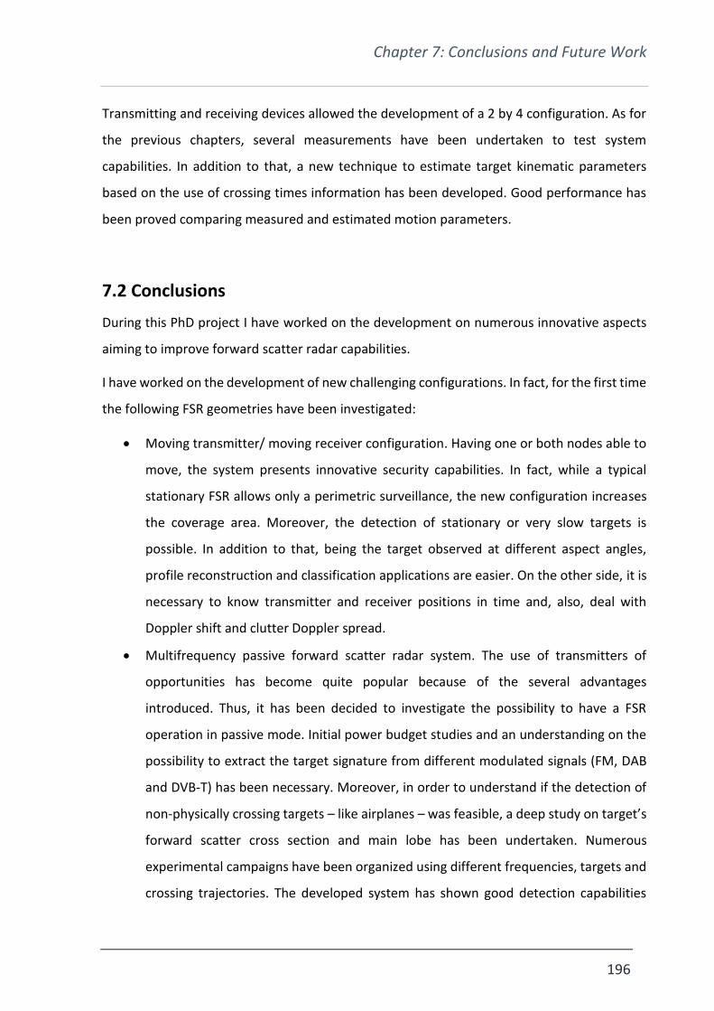
Chapter 7: Conclusions and Future Work
196
Transmitting and receiving devices allowed the development of a 2 by 4 configuration. As for
the previous chapters, several measurements have been undertaken to test system
capabilities. In addition to that, a new technique to estimate target kinematic parameters
based on the use of crossing times information has been developed. Good performance has
been proved comparing measured and estimated motion parameters.
7.2 Conclusions
During this PhD project I have worked on the development on numerous innovative aspects
aiming to improve forward scatter radar capabilities.
I have worked on the development of new challenging configurations. In fact, for the first time
the following FSR geometries have been investigated:
• Moving transmitter/ moving receiver configuration. Having one or both nodes able to
move, the system presents innovative security capabilities. In fact, while a typical
stationary FSR allows only a perimetric surveillance, the new configuration increases
the coverage area. Moreover, the detection of stationary or very slow targets is
possible. In addition to that, being the target observed at different aspect angles,
profile reconstruction and classification applications are easier. On the other side, it is
necessary to know transmitter and receiver positions in time and, also, deal with
Doppler shift and clutter Doppler spread.
• Multifrequency passive forward scatter radar system. The use of transmitters of
opportunities has become quite popular because of the several advantages
introduced. Thus, it has been decided to investigate the possibility to have a FSR
operation in passive mode. Initial power budget studies and an understanding on the
possibility to extract the target signature from different modulated signals (FM, DAB
and DVB-T) has been necessary. Moreover, in order to understand if the detection of
non-physically crossing targets – like airplanes – was feasible, a deep study on target’s
forward scatter cross section and main lobe has been undertaken. Numerous
experimental campaigns have been organized using different frequencies, targets and
crossing trajectories. The developed system has shown good detection capabilities

Chapter 7: Conclusions and Future Work
197
even with small crossing planes. Moreover, it has been possible to appreciate the
difference in using various frequencies. In fact, higher frequencies offer a more
accurate estimation of motion parameters whereas lower ones determine a wider
operational area. Therefore, a multifrequency operation would improve the system
performance.
• Multi input multi output forward scatter radar. Aiming to improve FSR capabilities and
overcome some limitations due to the specific geometry, a MIMO configuration has
been developed. In fact, while FSR is characterized by a narrow detection corridor, the
use of multiple transmitters and receivers would extend the detection area. A scaled
2 transmitters - 4 receivers configuration has been developed in order to test the
capabilities of the system. Power budget calculations have been required to determine
whether the radar would have performed well. Various experimental measurements
have been undertaken. Results have proved good system’s detection capability.
Information collected by the crossing of the multiple baselines have been used to
accurately estimate target motion parameters.
In addition to the listed new investigated configurations, I have focused on the development
of several techniques to estimate the target’s motion parameters.
• Target kinematic information estimated using the spectrogram. Frequency domain
target signature is just another way to look at the received target waveform. The
variation of the spectrogram according to different frequencies, target’s speed,
crossing angle and crossing point are clearly shown in this thesis. A comparison with
the previously developed processing proves that both techniques allow to estimate
motion of the target in an accurate way. However, this new processing operating in
frequency domain can be extremely useful when the time domain signature loses its
typical shape, like in highly cluttered scenario. In fact, the spectrogram appears to offer
a more robust representation of the target signature. Thus, even when the
surrounding clutter is strong or when the target fully shadows the receiving antenna,
the developed techniques is capable to estimate target’s motion parameters.
Therefore, this developed technique can be used to assist the time domain processing
to reduce the computational cost or to assist in difficult scenarios.

Chapter 7: Conclusions and Future Work
198
• Target motion parameter estimation technique in moving transmitter/ moving
receiver FSR. Due to the motion of both ends, the target signature changes in time.
Therefore, the time domain processing has been modified to include the movement of
transmitter and receiver. Tests on simulated and real data have shown the good
system capabilities in estimating motion parameters. Moreover, this new processing
allows to solve an important ambiguity stationary FSR is affected from. In fact, it is
possible to determine the target’s direction.
• Target kinematic parameters estimation based on crossing times in a multi input multi
output forward scatter radar. During the investigation of a MIMO FSR configuration,
an innovative technique to estimate target motion information has been developed.
Such processing is based on the use of the multiple baselines’ crossing times. The
technique has been tested on numerous experimental data and has proved an
extremely accurate estimation.
Finally, during my PhD project, I have focussed on the investigation of clutter and its effect in
a moving transmitter/ moving receiver configuration. In fact, due to the nodes’ motion,
Doppler shift and clutter Doppler spread were expected. To understand how the received
signature is affected by such issue, a highly adaptable model to simulate returns from the
surrounding has been developed. Simulations have been used to understand the effects of
vegetation clutter on a system operating at various frequencies and with a receiver moving at
different speeds and trajectories. Simulated data has been compared to experimental results
showing very good accordance.
7.3 Future work
This project has investigated several innovative FSR configurations and new techniques which
could improve the accuracy of this radar system. The proposed work can open to future
research possibilities:
• Improve developed target motion parameters estimation techniques. In fact, these
approaches have offered an accurate estimation of target’s speed. However, crossing
angle and crossing point information show a higher error.

Chapter 7: Conclusions and Future Work
199
• Improve target classification and profile reconstruction using MIMO and moving
transmitter/ moving receiver configurations.
• Develop a MIMO forward scatter operating with longer baselines and presence of
clutter.
• Investigate target detection in highly cluttered moving transmitter/ moving receiver
FSR. In fact, it has been shown in this document how the receiver motion introduces
Doppler shift and clutter Doppler spread that could deteriorate the system
performance.
• Develop a multifrequency multimode FSR network of moving and stationary
transceivers operating together for security applications.

Appendix A: Target Doppler Signature Extraction
200
Appendix A: Target Doppler Signature
Extraction Glossary of Abbreviations
LPF Low Pass Filter
SLD Square Law Detector
Target Doppler Signature Extraction
This appendix aims to show in detail how to extract of the target Doppler signature in forward
scatter radar. A concise description, sufficient to understand the material described in the
thesis, is presented in Chapter 2. However, for the eager reader, the full steps allowing to
obtain the target Doppler signature from received signal are here described.
The received signal in FSR is composition of the leakage signal tSLS , which is the one acquired
in absence of target, and the target signal tSTS , strictly referring to a scenario when the
target is crossing the baseline. The latter can be seen as a modulation of the former. It is
important to underline how both of the play a fundamental role in building the construction
of the FSR signature and therefore are both necessary. As a direct consequence of just said,
the signal at the input of the receiver can be expressed as
tStStS TSLSRI (A.1)
From [1] the shadow signal can be assumed being phase shifted by 2 respect to the leakage
signal. So, the previous relation can be expressed as
shTSLSRI ttAtAtS 00 sincos (A.2)
assuming the transmitter emits a sinusoidal wave with angular carrier frequency 0 . The
target signal is delayed by a time sht , due to a different path length. LSA and TSA are the
amplitude of leakage and target signal at the receiver, respectively.

Appendix A: Target Doppler Signature Extraction
201
The proposed procedure in order to extract the target Doppler signature is based on the use
of a self-mixing heterodyne receiver.
Figure A.1. Block diagram of the processing chain.
The block diagram of the processing chain required to extract the Doppler signature is shown
in Figure A.1. It consists in a square low detector (SLD) followed by a low pass filter (LPF).
Given a signal as the one in (A.2) at the input of the SLD, the first block is
ttAAtAtA
tAtAtS
DTSLSDTSLS
DTSLSRI
000
22
0
22
2
00
2
sincos2sincos
sincos (A.3)
with shD t0 the angular Doppler frequency.
Considering the following trigonometric identities
sinsin2
1cossin
2
2cos1sin
2
2cos1cos
2
2
(A.3) can be written as
ttAA
tA
tA
tS
DDTSLSD
TSLS
RI
sin2sin2
2cos1
2
2cos10
0202
2
(A.4)
Looking at (A.4), it is evident the signal at the output of the SLD is formed by components at:
• 0 frequency;
• double of the transmitted frequency
• Doppler frequency.
The low pass filter that follows the SLD block is inserted to eliminate the component at double
of the transmitted frequency. The cutting frequency is chosen according to the radar
application and the maximum target velocity expected.

Appendix A: Target Doppler Signature Extraction
202
The signal at the output of the receiver, tSRO , is then
tAAAA
tS DTSLSTSLS
RO sin2
22
(A.5)
The signal after the processing is composed of a DC component, 2
22
TSLS AA , representing the
power of the leakage path, and the phase signature having amplitude TSLS AA .
Finally, considering
LtRtR
tt
RxTx
c
LtRtRtshD RxTx
sh
2sin
sinsin 0
(A.6)
(A.5) can be expressed as
LtRtRAA
AAtS RxTx
TSLSTSLS
RO
2sin
2
22
(A.7)
where tRTx , tRRx , L and are the distance transmitter-target, target-receiver, the
baseline and the wavelength.

Appendix A: Target Doppler Signature Extraction
203
Bibliography
[1] R. E. Hiatt, K. M. Siegel, and H. Weil, ‘Forward Scattering by Coated Objects Illuminated by Short Wavelength Radar’, Proceedings of the IRE, vol. 48, no. 9, pp. 1630–1635, Sep. 1960.
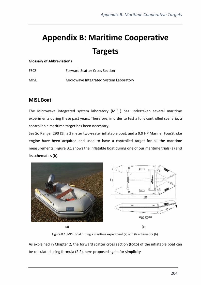
Appendix B: Maritime Cooperative Targets
204
Appendix B: Maritime Cooperative
Targets Glossary of Abbreviations
FSCS Forward Scatter Cross Section
MISL Microwave Integrated System Laboratory
MISL Boat
The Microwave integrated system laboratory (MISL) has undertaken several maritime
experiments during these past years. Therefore, in order to test a fully controlled scenario, a
controllable maritime target has been necessary.
SeaGo Ranger 290 [1], a 3 meter two-seater inflatable boat, and a 9.9 HP Mariner FourStroke
engine have been acquired and used to have a controlled target for all the maritime
measurements. Figure B.1 shows the inflatable boat during one of our maritime trials (a) and
its schematics (b).
(a) (b)
Figure B.1. MISL boat during a maritime experiment (a) and its schematics (b).
As explained in Chapter 2, the forward scatter cross section (FSCS) of the inflatable boat can
be calculated using formula (2.2), here proposed again for simplicity

Appendix B: Maritime Cooperative Targets
205
2
24
AFS
Figure B.2. Representation of the maritime target as combination of simple shapes.
Figure B.2 stylizes the MISL boat silhouette as combination of simple shapes, taking into
account the boat itself, one person driving and the engine. Therefore, using a simplified
approach A , the target silhouette, can be calculated as sum of all the simple geometries
shown in Figure B.2.
Inflatable Ball
Since the FSCS of a spherical target can be accurately calculated, in order to test the
performance of our system and to provide a calibration signature, an inflatable ball has been
used during some of the maritime measurements. The sphere has been towed by the MISL
boat using a rope approximately 10 m behind. As consequence of being towed, such target
moved with the same speed of the inflatable boat, giving the opportunity to test the
capabilities of our processing too. Figure B.3 shows the inflatable spherical target (a) and a
picture during one of our experiments, with the boat pulling the ball (b).

Appendix B: Maritime Cooperative Targets
206
(a)
(b)
Figure B.3. Spherical target (a) and a picture from a maritime experiment with the MISL boat pulling the inflatable ball.
Table B.1. Radar cross section values of our controlled targets.
Target Radar Cross Section
(At 7.36 GHz)
By formula (2.2) By CST
MISL boat 42.42 dBm2 42.60 dBm2
Spherical target 29.21 dBm2 29.40 dBm2
0.65 m

Appendix B: Maritime Cooperative Targets
207
Bibliography
[1] ’Boats & Tenders – Seago’ [Online] Available: http://www.seagoyachting.co.uk/ranger-290-p-26.html. [Accessed 04-Aug-2015], .
Appendix C: Maritime Equipment
208
Appendix C: Maritime Equipment Glossary of Abbreviations
LNA Low Noise Amplifier
MISL Microwave Integrated System Laboratory
PRF Pulse Repetition Frequency
VSWR Voltage Standing Wave Ratio
Maritime FSR Equipment
The Microwave integrated system laboratory (MISL) has undertaken several experimental
campaigns in maritime environment. Therefore, it has arisen the necessity to develop a
dedicated, practical, portable and easy to deploy forward scatter system to use in such a
scenario.
The equipment composed of a transmitting and a receiving node is shown in Figure C.1. As
visible, both Tx and Rx fit in portable, waterproof, dustproof and crushproof ‘Pelican 1500’
cases [1]. A lightweight 12V lithium-polymer battery with 22Ah capacity supplies each node.
Temperature inside the cases is reduced using a heatsink pad and a metal plate underneath
the equipment. In addition, a hole on the bottom part of the case is used to put the cables
outside the box. Each case has been provided with a pole holder allowing to mount an
adjustable pole to hold omnidirectional antennas.
Figure C.2 shows the system block diagram of the 7.36 GHz FSR device.
Transmitter
The transmitter comprises a low cost wave generator developed by Dr. Hoare in the MISL
laboratories. The system works at 7.36 GHz and can be set to operate in CW or pulsed mode,
transmitting a 30 MHz, 100 MHz or 1 GHz bandwidth Gaussian modulated pulse. Furthermore,
the pulse repetition frequency (PRF) can be adjusted by a hardware switch.

Appendix C: Maritime Equipment
209
(a) (b)
Figure C.1. Transmitter (a) and receiver (b) devices.
The generated signal goes through a Mini Circuits ZVA 183+[2] power amplifier characterized
by a 26 dB gain. The transmitter output power is 26 dBm. Tx can also be used as a standalone
device.
Figure C.2. Transmitter and receiver block diagram.
Receiver
The receiver comprises a first Hittite HMC-001 LNA followed by a combination of other four
identical LNAs. In order to eliminate contributed at not desired frequencies, one high and low
band pass filters are insert. Moreover, in order to extract the Doppler signature, the signal is
processed using a sequence of log detector, low pass filter and ADC. Finally, the extracted
target signature is collected by a laptop connected to the receiver.

Appendix C: Maritime Equipment
210
Antennas
Two different kinds of antennas have been used in our measurements, depending on the
purpose of the tests: directional and omnidirectional antennas.
The majority of our experiments have been undertaken using two Flann Standard gain horn
antennas Series 240 [3], Figure C.3. The purchased model was the 15240, operating from 6.58-
10 GHz with a 20 dB standard mid-band gain .Such antennas have a 20 degrees bandwidth in
both planes.
Figure C.3. Tx and Rx units equipped with horn antennas.
In order to test the performance of our equipment, omnidirectional antennas have been used
too. Such antennas have been designed and manufactured by Dr. Vladimir Sizov in the MISL
laboratories. The antenna design is shown in Figure C.4
Figure C.4. Omnidirectional antennas.
The voltage standing wave ratio (VSWR) of such prototype antennas is shown in Figure C.5.
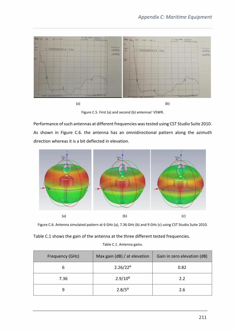
Appendix C: Maritime Equipment
211
(a) (b)
Figure C.5. First (a) and second (b) antennas’ VSWR.
Performance of such antennas at different frequencies was tested using CST Studio Suite 2010.
As shown in Figure C.6. the antenna has an omnidirectional pattern along the azimuth
direction whereas it is a bit deflected in elevation.
(a) (b) (c)
Figure C.6. Antenna simulated pattern at 6 GHz (a), 7.36 GHz (b) and 9 GHz (c) using CST Studio Suite 2010.
Table C.1 shows the gain of the antenna at the three different tested frequencies.
Table C.1. Antenna gains.
Frequency (GHz) Max gain (dB) / at elevation Gain in zero elevation (dB)
6 2.26/22⁰ 0.82
7.36 2.9/10⁰ 2.2
9 2.8/5⁰ 2.6

Appendix C: Maritime Equipment
212
Bibliography
[1] ‘1500EMS Protector - Medium Case | EMS Case | Pelican Professional’, Pelican Products, Inc. [Online]. Available: http://www.pelican.com/pro/product/watertight-protector-hard-cases/medium-case/ems-case/1500EMS/’. [Accessed: 15-Aug-2017].
[2] ’ZVA-183+’ [Online]. Available: https://ww2.minicircuits.com/pdfs/ZVA-183+.pdf [Accessed: 16-Aug-2017], .
[3] ’Standard Gain Horns Series 240’. [Online]. Available: https://flann.com/wp-content/uploads/2016/01/Series-240.pdf [Accessed: 16-Aug-2017], .

Appendix D: Clutter Measurement Equipment
213
Appendix D: Clutter Measurements
Equipment Glossary of Abbreviations
ADC Analogue-to-Digital Converter
FSR Forward Scatter Radar
RSSI Received Signal Strength Indicator
Rx Receiver
Tx Transmitter
Clutter FSR Equipment
A multi-frequency transmitter (Tx) and receiver (Rx) forward scatter radar (FSR) has been used
for the undertaken clutter measurements. Such prototype was built in the Microwave
Integrated System Laboratory (MISL) by Dr Vladimir Sizov with the aim of having a robust,
waterproof, compact and extremely portable device for the group’s projects.
(a) (b)
Figure D.1. Four channels transmitter (a) and receiver (b).

Appendix D: Clutter Measurement Equipment
214
Figure D.1 shows the transmitter (a) and receiver (b) nodes. They both operate at 64, 135, 173
and 434 MHz. Tx transmits four continuous waves (CW) at the different carriers which are
then captured by the receiving antennas and processed by a laptop connected to Rx.
The simplified block diagram of the equipment is proposed in Figure D.2. Rx is connected to a
PC by extended USB cables to acquire data from analogue-to-digital converters (ADC) and
store received data files. Battery state indicator (LED) shows TX “Power ON” state and “Battery
low” (flashing LED) state as well.
Figure D.2. Equipment block diagram.
Tx and Rx are built from Radio Metrix’s modules installed on carrier boards and utilize
Panorama’s antennas presented in Figure D.3. Looking form left to right the 64, 135, 434 and
173 MHz antennas are shown.
Figure D.3. Four omnidirectional antennas used with the prototype.
The antenna’s specifications are presented here.

Appendix D: Clutter Measurement Equipment
215

Appendix D: Clutter Measurement Equipment
216
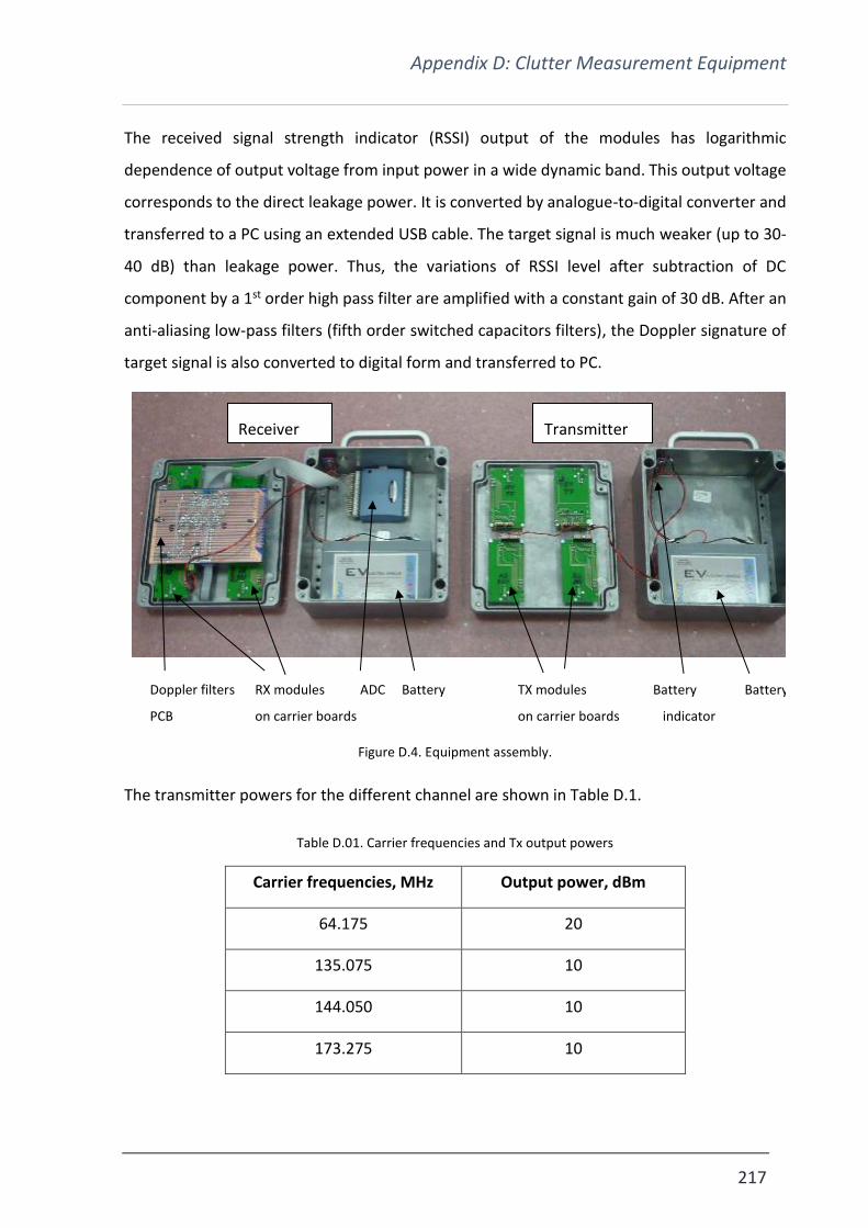
Appendix D: Clutter Measurement Equipment
217
The received signal strength indicator (RSSI) output of the modules has logarithmic
dependence of output voltage from input power in a wide dynamic band. This output voltage
corresponds to the direct leakage power. It is converted by analogue-to-digital converter and
transferred to a PC using an extended USB cable. The target signal is much weaker (up to 30-
40 dB) than leakage power. Thus, the variations of RSSI level after subtraction of DC
component by a 1st order high pass filter are amplified with a constant gain of 30 dB. After an
anti-aliasing low-pass filters (fifth order switched capacitors filters), the Doppler signature of
target signal is also converted to digital form and transferred to PC.
Figure D.4. Equipment assembly.
The transmitter powers for the different channel are shown in Table D.1.
Table D.01. Carrier frequencies and Tx output powers
Carrier frequencies, MHz Output power, dBm
64.175 20
135.075 10
144.050 10
173.275 10
Receiver Transmitter
Doppler filters RX modules ADC Battery TX modules Battery Battery
PCB on carrier boards on carrier boards indicator

Appendix D: Clutter Measurement Equipment
218
All RX channels have similar sensitivity and linear detection range approximately, shown in
Figure D.5.
Figure D.5. Receivers detection range.
Recorded data
Data is recorded using a MathCAD code written by Dr Vladimir Sizov. Such program allows to
extract and display the signals received by the device. Thus, in order to acquire such data three
steps here listed have to be followed:
• Connect the receiver to a computer;
• Open Instacal in order to enable the PC to detect the device;
• Open the MathCAD code, set some initial parameters such as: file name, acquisition
time and sampling frequency numbers of samples and sampling rate;
After these steps, it is possible to start the acquisition. The MathCAD acquisition control
window is shown in Figure D.6
140 130 120 110 100 90 80 70 60 500.5
1
1.5
2
2.5
140 130 120 110 100 90 80 70 60 500.5
1
1.5
2
2.5
140 130 120 110 100 90 80 70 60 500.5
1
1.5
2
2.5
140 130 120 110 100 90 80 70 60 500.5
1
1.5
2
2.5
140 130 120 110 100 90 80 70 60 500.5
1
1.5
2
2.5
140 130 120 110 100 90 80 70 60 500.5
1
1.5
2
2.5
Linear detection range
Input Power, dBm
RSS
I ou
tpu
t, V
135
173
64
434
Range used
for baselines 50-400 m

Appendix D: Clutter Measurement Equipment
219
Figure D.6. Screenshot from the MathCAD code used to acquire the data.

Appendix D: Clutter Measurement Equipment
220
Bibliography
[1] ‘1500EMS Protector - Medium Case | EMS Case | Pelican Professional’, Pelican Products, Inc. [Online]. Available: http://www.pelican.com/pro/product/watertight-protector-hard-cases/medium-case/ems-case/1500EMS/’. [Accessed: 15-Aug-2017].
[2] ’ZVA-183+’ [Online]. Available: https://ww2.minicircuits.com/pdfs/ZVA-183+.pdf [Accessed: 16-Aug-2017], .
[3] ’Standard Gain Horns Series 240’. [Online]. Available: https://flann.com/wp-content/uploads/2016/01/Series-240.pdf [Accessed: 16-Aug-2017], .

Appendix E: USRP 2950R
221
Appendix E: USRP 2950R Glossary of Abbreviations
GPSDO GPS Disciplined Oscillator
SDR Software Defined Radio
USRP 2950R
The National Instrument USRP-2950R [1] (Figure E.1) is a device of a family of RF hardware,
called software defined radio (SDR). It comprises two transceivers channels enabling to
transmit and receive signals from 50 MHz up to 2.2 GHz. A GPS-disciplined oscillator (GPSDO)
is included to provide high precision timing and synchronization.
The device is characterized by a maximum transmitted power of +15 dBm, a maximum
amplification of +31.5 dB and a maximum RF bandwidth of 40 MHz.
For more detailed schematics and description see [2].
Figure E.1. NI USRP-2950R.
The USRP can be connected to a host computer in three different ways:
• 1 Gbit Ethernet. It is an easy and quick method but limits the RF bandwidth to 10 MHz
and the maximum data flow to 125 MBps;
• ExpressCard. It limits the bandwidth to 20 MHz. On the other hand it allows to control
the device by laptop, allowing system’s mobility;
• PCI x4 card. It gives the possibility of operate with the full bandwidth but it allows to
control the device only by desktop.

Appendix E: USRP 2950R
222
The motherboard contains a Xilinx Kintex-7 FPGA allowing initial signal processing and
therefore simplifying the post processing.
During typical operation of the device, the parameters of the acquisition – sampling rate,
centre frequency and gain of the integrated LNAs, are set by the user, along with other
parameters of the system, such as buffer length, clock reference (note that GPSDO is used as
reference source for further stability of the receiver and recording of the time stamp of the
recording). LabVIEW is used to control the USRP. A screenshot of the front-view of the
software is shown in Figure E.2.
Figure E.2. LabVIEW screenshot.

Appendix E: USRP 2950R
223
Bibliography
[1] ‘Overview of the NI USRP RIO Software Defined Radio - National Instruments’. [Online]. Available: http://www.ni.com/white-paper/52119/en/. [Accessed: 15-Oct-2017].
[2] ‘USRP Hardware Driver and USRP Manual: Table Of Contents’. [Online]. Available: https://files.ettus.com/manual/. [Accessed: 18-Oct-2017].