1

REVISTA INVESTIGACION OPERACIONAL VOL. xx , NO.x, xxx-xxx, 201x

FORTHCOMINGPAPER·#90b05-18-02

OPTIMAL PRODUCTION INTEGRATED INVENTORY MODEL WITH QUADRATIC DEMAND FOR DETERIORATING ITEMS UNDER INFLATION USING GENETIC ALGORITHM Isha Talati and Poonam Mishra

* Faculty, Department of Mathematics & Computer Science, School of Technology, Pandit Deendayal Petroleum University.

ABSTRACT: This paper is a production integrated inventory model between manufacturer and retailer with quadratic demand and time dependent deterioration. Paper also considers effect of inflation on total cost. Manufacturer offers lot size dependent ordering cost to boost higher orders as well as it decreases manufacturer’s inventory holding cost significantly. Total cost of model is obtained using both classical optimization technique and genetic algorithm. Results clearly show that GA has succeeded in obtaining global minimum whereas classical method has stuck with local minimum. For using classical optimization technique we have used Maple 18 whereas for genetic algorithm we have used MATLAB R2013a.The optimal solution of this model is illustrated using numerical example. Sensitivity for inflation and other parameters of demand has been carried out to analyse their effect on total cost. This paper will encourage researchers involve in inventory and supply chain management to optimize complex problems using different evolutionary search algorithm in order to reach to global optimum. KEYWORDS: Integrated inventory, time dependent deterioration, genetic algorithm, lot size dependent ordering cost, time dependent quadratic demand, inflation MSC: 90B05 RESUMEN: Este documento es un modelo de inventario integrado de producción entre el fabricante y el minorista con demanda cuadrática y deterioro dependiente del tiempo. El documento también considera el efecto de la inflación en el costo total. El fabricante ofrece un costo de pedido dependiente del tamaño del lote para impulsar pedidos más altos y también disminuye significativamente el costo de mantenimiento del inventario del fabricante. El costo total del modelo se obtiene utilizando la técnica de optimización clásica y el algoritmo genético. Los resultados muestran claramente que GA ha logrado obtener el mínimo global mientras que el método clásico se ha quedado con el mínimo local. Para utilizar la técnica de optimización clásica, hemos utilizado Maple 18, mientras que para el algoritmo genético hemos utilizado MATLAB R2013a. La solución óptima de este modelo se ilustra mediante un ejemplo numérico. La sensibilidad para la inflación y otros parámetros de la demanda se han llevado a cabo para analizar su efecto sobre el costo total. Este documento alentará a los investigadores a participar en el inventario y en la gestión de la cadena de suministro para optimizar problemas complejos utilizando diferentes algoritmos de búsqueda evolutiva con el fin de alcanzar el óptimo global. PALABRAS CLAVE: Inventario integrado, deterioro dependiente del tiempo, algoritmo genético, tamaño del lote dependiente del costo de la orden, demanda cuadrática dependiente del tiempo, inflación

1. INTRODUCTION

Till a recent past every member of supply chain was managing its own inventory in isolation and minimizes its cost individually. But later researchers realised that optimization of cost or profit with respect to only one member could be at the cost of other members. This will not lead to a long term authentic inventory model. Therefore researchers started proposing integrated model where joint profit or cost is optimized and at the same time individual profits are studied. Goyal (1976): firstly made integrated model for single supplier and single customer so that either both the parties get economical benefit or no one at least get loss. Banerjee (1986): extended that model for joint optimal total cost for purchaser and vendor. Goyal & Gunasekaran (1995): formulated joint optimal model for deteriorating items. Rau et al. (2006): extended optimal total cost among the supplier, the producer, and the buyer. Cárdenas-Barrón et al. (2011): optimized integrated

2

inventory model using arithmetic–geometric inequality. Chung & Cárdenas-Barrón (2014): formulated two-echelon model using promotional tool when demand depends on sales team’s initiatives. Sarkar et al. (2014): generated model for defective items in case of payment delay. Sarkar (2016): formulated quantity discount model for shortages with three stage inspection. Shah et al. (2017): generated model for multi-items with up-stream permissible delay. Managing inventory of deteriorating items electronic products, medicines and fashion accessories that loses their utility and demand with time or perishable items with very less shelf life like dairy products, fish, meat, vegetables, etc. is not an easy task. Researchers have already studied effect of deterioration using different governing functions. Classical EOQ model was firstly assumed for exponentially deteriorating items by Ghare & Schrader (1963): Covert & Philip (1973): formulated model for items that follow two parameter Weibull distributiomn. Philip (1974): generalized that model. Patil & Patel (2013): extended that for linear demand under inflation. Mohan and Venkateswarlu (2013a, 2013b, 2013c, 2014): extended that model for quadratic demand using different promotional tools. Classical optimization techniques either unable to address complex multi-variable non-linear problems or stuck with local optimum. For this type of problems researchers are using various heuristic search algorithms like genetic algorithm, particle swam optimization and simulated annealing. Genetic algorithm is based on the natural selection process of nature in which next generation is always better than the previous one. Solutions get fitness score in the basis of fitness function and slowly with iterations all the possible solutions move towards global optimum. Goldberg (1989): introduces principle and algorithm of GA. Since then it has been used in the wide variety of problems for optimization. Murata et al. (1996):, Goren (2008):, Radhakrishnan at el. (2009):, Radhakrishnan at el. (2010):, Narmadha et al. (2010):, Woarawichai (2012): , Mishra and Talati (2015): etc have used genetic algorithm to solve their optimization problems. Inflation plays an important role in inventory management as it may happen in the case of long cycle times that the actual value of the revenue is too less than it seems to be. Thus, role of inflation must be studied for long term inventory supply chain models. Sarkar & Pan (1994): formulated model under shortages. Sarkar et al. (2010): extended that model with permissible delay in payment. Shah & Shukla (2010): generated model for order linked trade credit. Shah & Vaghela (2016): formulated model for an imperfect production with effort dependent demand. Shah & Vaghela (2017): explained model with an advertisement dependent demand. All the above mentioned papers has studied integrated supply chain system either without deterioration or with constant deterioration but our proposed model has considered time dependent deterioration with the effects of inflation. Moreover, unlike above mentioned papers we have just not solved the problem with analytical approach but also analysed it with Genetic Algorithm due to complexity of the problem. In this paper we have considered supply chain of single manufacturer and single retailer for items that deteriorate with respect to time and follow Weibull distribution. Demand is time dependent and quadratic in nature and model is studied under inflation. We have optimized our problem using classical optimization technique and genetic algorithm. Sensitivity analysis of important demand parameters is carried out to study its effect on the total cost.

2. ASSUMPTIONS AND NOTATIONS: 2.1 Notations

Inventory parameters for manufacturer

mA Set up costs($):

mh Holding cost / unit / annum($):

P

Production rate (and known):

1b Deteriorating cost /unit ($):

γ

Salvage cost/unit ($):

mTC

Total cost for manufacturer($):

Inventory parameters for retailer oC Fix ordering cost($):

rQ Retailer’s order quantity per order

T Cycle time(Years):

3

rh Holding cost for retailer($):

( )tθ Time dependent deterioration of Inventory follows Weibull distribution

rTC Total cost for retailer($):

r Rate of inflation TC T η

Joint total cost($): Cycle time (Decision variable): Lot size parameter (Decision variable):

2 .2. Assumptions 1. Considered system with single manufacturer and single retailer for a single item. 2. The demand rate ( )D t at time t is assumed to be ( ) 2; 0, 0, 0D t a bt ct a b c= + + ≥ ≠ ≠ . Here a is initial rate of demand.

b is the rate with which demand rate is increases. c is the rate with which the change in the rate demand rate itself increases. 3. Shortages are not allowed and lead time is zero. 4. The production rate is constant say ( ),P P D t> 5. Ordering cost is lot size dependent. 6. System’s inventory depleted with respect to time and follow Weibull distribution. ( ) 1 ; 0< <1, 1,t>0t tβθ αβ α β−= ≥

7. Deteriorating items are neither repaired nor replaced during cycle time T. 8. The effect of inflation and time value of money are considered. 3. MATHEMATICAL MODEL 3.1. Manufacturer’s present worth total cost The on hand inventory of manufacturer depletes with demand and deterioration. Then the governing equation of inventory at any time t is given by

( ) ( ); 0 t Tmm

dQt Q P D t

dtθ= − + − ≤ ≤

(1):

Solving equation (1): using boundary conditions ( )0 0 mQ = we get

( ) ( )2 3

2 3mbt ctQ t P a t= − − −

(2):

Using ( )Qm mT Q= we get total quantity produce by manufacturer per cycle is

( )2 3

2 3mbT cTQ P a T= − − −

(3):

Basic costs associated with manufacturer • Set-up Cost

m mSC A= (4):

• Holding Cost

( )0

Trt

m m mHC h Q t e dt−= ∫

( ) ( )2 34 3 5 4

2 12 6 3 15 8mP a T P a rTcT bT crT brTh

⎛ ⎞− −⎜ ⎟= − − − − +⎜ ⎟⎝ ⎠

(5):

4

Number of deteriorating items

( )0

( )T

rtm mDE T Q D t e dt−= − ∫

(6):

• Deteriorating Cost ( )1m mDC b DE T= (7):

• Salvage Cost ( )1m mSV b DE Tγ= (8):

So total present worth total cost for manufacturer is

( )m m m m mTC T SC HC DC SV= + + − (9):

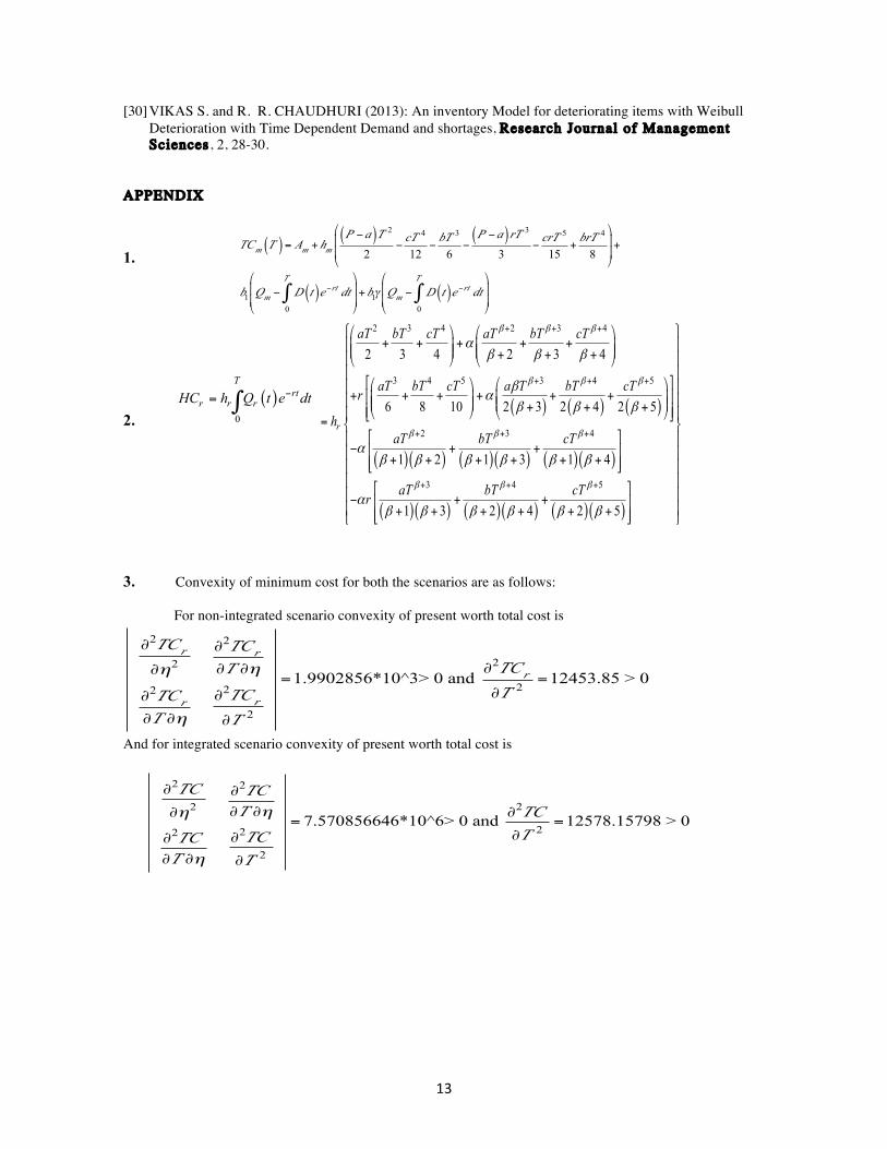
(Refer Appendix 1 for TC m(T): equation): 3.2. Retailer’s present worth total cost Here we take demand and deterioration both times dependent. So on hand inventory of retailer at any time t is given by differential equation

( ) ( ) ; 0 t Trr

dQ t Q D tdt

θ+ = − ≤ ≤ (10):

Using boundary condition ( ) 0rQ T = and ignoring higher term of α and r we get

(11):

and use ( )0r rQ Q= we get

1 2 32 3

2 3 1 2 3rb c aT bT cTQ aT T T

β β β

αβ β β

+ + +⎛ ⎞⎛ ⎞= + + + + +⎜ ⎟⎜ ⎟ ⎜ ⎟+ + +⎝ ⎠ ⎝ ⎠

(12):

Basic costs associated with retailer

• Ordering cost is lot size dependent so

0 ,0 < < 1r rOC C Qη η= (13):

• Holding cost

( )0

Trt

r r rHC h Q t e dt−= ∫ (14):

(Refer appendix 2):

Qr t( ) = 1+αt β( ) a T − t( )+ b2 T2 − t 2( )+ c3 T

3 − t 3( )⎛

⎝⎜

⎞

⎠⎟

⎡

⎣⎢⎢

⎤

⎦⎥⎥+

αaβ +1

T β+1 − t β+1( )+ bβ + 2

T β+2 − t β+2( )+ cβ +3

T β+3 − t β+3( )⎡

⎣⎢

⎤

⎦⎥

5

• Number of deteriorating units

( ) ( )0

Trt

r rDE T Q D T e dt−= − ∫

(15):

• Deteriorating cost ( )1r rDC b DE T= (16):

• Salvage cost ( )1r rSV b DE Tγ= (17):

So retailer present worth of total cost is

( ),r r r r rTC T OC HC DC SVη = + + − (18):

3.3. Joint present worth total cost System present worth of total cost is

( ) ( ) ( ), ,m rTC T TC T TC Tη η= + (19):

4. COMPUTATIONAL ALGORITHMS We have three objective functions: Present worth of total cost of manufacturer, retailer and joint for system. We optimize those using analytical and Genetic algorithm. Set numerical values for different parameters except for decision variables and T η . 4.1. Analytical Algorithm

1. Calculate optimal cycle time *T from 0mTCT

∂=

∂

2. Using optimal cycle time obtain optimal lot size and present worth total cost for manufacturer.

3. Find optimal *T and *η from 0 and 0r rTC TCT η

∂ ∂= =

∂ ∂ simultaneously.

4. Using *T and *η compute optimal lot size and present worth total cost for retailer.

5. Obtain *T and *η from 0 and 0TC TCT η

∂ ∂= =

∂ ∂ simultaneously.

6. Using *T and *η compute optimal lot size and present worth total cost for manufacturer, retailer and hence for system.

4.4. Genetic Algorithm

1. Start with an initial population of 30 chromosomes. 2. Get there fitness score to rank them. 3. Chromosomes will get entry in mating pool on the basis of their fitness score using rank selection method. 4. Perform stochastic uniform crossover for reproduction. Crossover fraction is considered 0.8 and 2-Elites are considered at each generation. 5. Again rank members of new generation by their fitness function and select members which can create next generation. 6. Perform step 3 and step 4 till absolute difference between two successive members is negligible i.e 1i ix x+ − < tolerance

5. NUMERICAL EXAMPLES AND SENSITIVITY ANALYSIS

6

Example: Consider inventory and supply chain parameters

1 01000, b = 1.5, c = 2.5, = 0.1, = 1.5, = 0.1($), P = 3000, A 200($), b 0.1($), C 2($), 2($ / ), h 2($ / )

m

m r

ah unit unit

α β γ= = = =

= =

Using analytical method we get results that shown in Table-1

Table-1: Computational results obtain using analytical approach Non-integrated scenario Integrated scenario

Optimal cycle time 0.162 0.2

Optimal eta 0.135 0.184

Optimal quantity 277 284

Manufacturer’s total cost 595.91 590.253

Retailer’s total cost 432.66 358.352

System total cost 1028.57 948.605

(Refer Appendix 3 for convexity of analytical solution): Results obtained for the same scenario using genetic algorithm is given in Table-2. Best fitness function for non-integrated scenario using genetic algorithm took 25 iterations for manufacturer and 14 iterations for retailer. Those best fitness plot shown in Figure 1 and Figure 2 respectively. And for integrated scenario genetic algorithm took 20 iterations. It’s best fitness plot is given in Figure 3.

Table-2: Computational results obtain using genetic algorithm Non-integrated scenario Integrated scenario Optimal cycle time 0.1 0.2 Optimal eta 0.242 0.2 Optimal quantity 242 262 Manufacturer’s total cost 541.883 510.182 Retailer’s total cost 323.872 133.593 System total cost 865.755 643.775

Figure 1: Best fitness solution for manufacturer’s present worth total cost in non-integrated scenario

7

Figure 2: Best fitness solution for retailer’s present worth total cost in non-integrated scenario

Figure 3: Best fitness solution for system’s present worth total cost in integrated scenario

Sensitivity Analysis: Sensitivity analysis is carried out for above example Case-(i): Accelerated growth model: If 0 and c 0 b > > , demand increases rapidly which is shown in Figure 4. Further, sensitivity of different parameters in this case is shown in Table 3.

Table-3: Sensitivity analysis for accelerated growth model Parameters Iterations *T *η

TC($):

α

0.1 51 0.2 0.2 643.775 0.2 51 0.2 0.2 643.818 0.3 51 0.2 0.2 643.830 0.4 51 0.2 0.2 643.841 0.5 52 0.2 0.2 643.879

β 1.5 51 0.2 0.2 643.775 2.0 54 0.2 0.19 643.438 2.5 51 0.2 0.198 643.368

8

3.0 52 0.2 0.196 642.903 3.5 51 0.2 0.194 642.803

r

0.1 51 0.2 0.2 643.775 0.2 51 0.2 0.2 642.484 0.3 54 0.2 0.2 641.018 0.4 52 0.2 0.2 639.622 0.5 51 0.2 0.284 638.622

Figure 4: Demand verses Time in accelerated growth model Case-(ii): Accelerated decline model: If 0 and c 0 b < < , demand decrease rapidly which is shown in Figure 5. Further, sensitivity of different parameters in this case is shown in Table 4.

0.5 1 1.5 2.52 3

100

200

300

400

Time

Demand

Time

Demand

0.5 1 1.5 2.52 3

200

300

400

100

9

Figure 5: Demand verses Time in accelerated decline Table-4: Sensitivity analysis for accelerated decline model

Parameters Iterations *T *η TC

α

0.1 51 0.2 0.2 642.511 0.2 51 0.2 0.2 642.481 0.3 51 0.2 0.2 642.458 0.4 51 0.2 0.2 642.431 0.5 51 0.2 0.2 642.408

β

1.5 51 0.2 0.2 642.511 2.0 51 0.198 0.221 642.415 2.5 51 0.197 0.2 642.395 3.0 51 0.195 0.2 642.382 3.5 51 0.192 0.2 642.376

r

0.1 51 0.2 0.2 642.511 0.2 51 0.2 0.2 633.356 0.3 52 0.2 0.2 630.568 0.4 51 0.2 0.2 624.507 0.5 51 0.2 0.2 618.545

Case-(iii): Retarded growth model: If

0 and c > 0 b < , demand slightly decreasing but then rapidly

increase which is shown in Figure 6. Further, sensitivity of different parameters in this case is shown in Table 5.

0.5 1 1.5 2.52 3

100

200

300

400

Time

Demand

10

Figure 6: Demand verses time in retarded growth model

Table-5: Sensitivity analysis for Retarded growth model Parameters Iterations *T *η

TC

α

0.1 51 0.2 0.2 642.501 0.2 51 0.2 0.2 642.495 0.3 51 0.2 0.2 642.439 0.4 51 0.2 0.2 642.426 0.5 51 0.2 0.2 642.400

β

1.5 51 0.2 0.2 642.501 2.0 51 0.21 0.2 642.439 2.5 51 0.22 0.2 642.375 3.0 51 0.23 0.2 642.280 3.5 51 0.2358 0.2 642.192

r

0.1 51 0.2 0.2 642.501 0.2 51 0.2 0.2 642.374 0.3 52 0.2 0.212 639.951 0.4 51 0.2 0.2 639.589 0.5 51 0.2 0.2 638.125

Case-(iv): Retarded decline model: If

0 and c < 0 b > , demand slightly increasing but then rapidly decrease. which is shown in Figure 7. Sensitivity of different parameters in this case is shown in Table 6.

Figure 7: Demand verses time in retarded decline model

Table-6: Sensitivity analysis for retarded decline model Parameters Iterations *T *η

TC

α

0.1 51 0.2 0.212 642.431 0.2 51 0.2 0.2 642.458 0.3 51 0.21 0.198 642.489 0.4 51 0.214 0.195 643.251 0.5 51 0.219 0.184 643.554

β

1.5 51 0.2 0.212 642.431 2.0 51 0.2 0.2156 642.692 2.5 51 0.2 0.2158 642.744 3.0 51 0.2 0.222 643.024

0.5 1 1.5 2.52 3

100

200

300

400

Time

Demand

11

3.5 51 0.2 0.231 643.524

r

0.1 51 0.2 0.212 642.431 0.2 53 0.2 0.2 642.244 0.3 51 0.2 0.2 641.581 0.4 51 0.2 0.2 641.123 0.5 51 0.2 0.2 640.842

The outcomes from sensitivity analysis are as follow.

• For accelerated growth model As scale parameter increase present worth of total cost increase with same optimal cycle time T and order power η As shape parameter increase present worth of total cost and optimal cycle time decrease with same optimal order power η

As inflation increase present worth of total cost decrease with keeping optimal cycle time T and order power η • For accelerated decline model As scale parameter increase present worth of total cost increase with same optimal cycle time T and order power η As shape parameter increase present worth of total cost and optimal cycle time decrease with same optimal order power η As inflation increase present worth of total cost decrease with keeping optimal cycle time T and order power η • For retarded growth model As scale parameter increase present worth of total cost decrease with same optimal cycle time T and order power η As shape parameter increase present worth of total cost decrease and optimal cycle time increase with same optimal order power η As inflation increase present worth of total cost decrease with keeping optimal cycle time T and order power η • For retarded decline model As scale parameter increase present worth of total cost increase with increasing in optimal cycle time T and decreasing in optimal order power η As shape parameter increase present worth of total cost increase and with increasing optimal order power η while optimal cycle time remain constant. As inflation increase present worth of total cost decrease with keeping optimal cycle time T and order power η .

6 . CONCLUSIONS In this paper, we have developed an integrated production inventory model for time dependent deteriorating units when demand rate follows time dependent quadratic function under inflation. To make model more authentic and usable lot size dependent ordering cost is being assumed. Total system cost as well as cost of individual players has been studied. The most important part of the paper is that model has been optimized using both classical optimization technique and genetic algorithm. Major conclusion of the paper is that GA approaches to global minimum whereas analytical method got stuck with local minimum for the problem discussed in the Mathematical model. Effect of demand parameters and inflation towards total cost is studied. Model is illustrated with a numerical example to illustrate present worth of total cost is less in genetic algorithm as compared to classical optimization technique. Sensitivity analysis of shape parameter, scale parameter and inflation with respect to demand rate is carried out.

RECEIVED: DECEMBER, 2017 REVISED : MAY, 2018

REFERENCES

[1] BANERJEE, A. (1986):A joint economic-lot-size model for purchaser and vendor. Decision Sciences,

17, 292-311 [2] CÁRDENAS-BARRÓN, L. , WEE, H. and BLOS, M. (2011): Solving the vendor–buyer integrated

inventory system with arithmetic–geometric inequality. Mathematical and Computer Modelling, 53, 991-997.

[3] CÁRDENAS-BARRÓN, L. E., and SANA, S. S. (2014): A production-inventory model for a two-echelon supply chain when demand is dependent on sales teams׳ initiatives, International Journal of Production Economics, 155, 249-258

[4] COVERT, R.B., and PHILIP, G. S. (1973): An EOQ model with Weibull distribution deterioration, AIIE Transaction, 5, 323-326.

[5] GHARE, P.M., and SCHRADER, G. F. (1963): A model for an exponentially decaying inventory, Journal of Industrial Engineering , 14, 238-243

12

[6] GOLDBERG, D. E. (1989): Genetic Algorithms in Search, Optimization and Machine Learning , Addison-Wesley, N. York.

[7] GOYAL, S. and GUNASEKARAN, A. (1995): An integrated production –inventory–marketing model for deteriorating items. Computers & Industrial Engineering, 28,755 –762.

[8] GOYAL, S. (1976): An integrated inventory model for a single supplier-single customer problem. International Journal of Production Research, 15, 107-111.

[9] MISHRA, P., and TALATI, I.(2015): A Genetic Algorithm Approach for an Inventory Model when Ordering Cost is Lot Size Dependent. Int. J. of Latest Tech. in Eng., Man. & App. Sci .,4, 92-97.

[10] MOHAN R. and VENKATESWARLU R., (2013b): Inventory Model for Time Dependent Deterioration, Time Dependent Quadratic Demand and Salvage Value, Journal of In. Math. Socy, 81, 135-146

[11] MOHAN R. and VENKATESWARLU R., (2013c): Inventory Management Model with Quadratic Demand, Variable Holding Cost with Salvage value, Res J of Management Sci. 2, 202-222

[12] MOHAN R. and VENKATESWARLU R., (2014): Weibull Deterioration, Quadratic Demand under Inflation, IOSR Journal of Mathematics. 10, 109-117

[13] MOHAN R. and VENKATESWARLU R.,(2013a): : Inventory Management Models with Variable Holding Cost and Salvage Value, IOSR J. of Busi. and Mgmt (IOSR-JBM):, 12, 37-42

[14] MURATA, T., H. ISHIBUCHI ,H., TANAKA(1996): Multi – objective algorithm and its applications to Flow shop Sheduling. Com. and Indu. Eng., 30, 954 – 968,

[15] NARMADHA. S, SELLADURAI. V, and SATHISH. G.(2010): Multiproduct Inventory Optimization using Uniform crossover Genetic algorithm, IJCSIS, 7(1).

[16] PATIL, S. S. and PATEL R. (2013):, An Inventory Model for Weibull Deteriorating Items with Linear demand, Shortages under permissible delay in Payments and inflation, International Journal of Mathematics and Stastist ics Invention, 1, 22-30

[17] PHILIP, G.C. (1974): A generalized EOQ model for items with Weibull distribution, AIIE Transaction, 6, 159-162.

[18] RADHAKRISHNAN. P, PRASAD V. M. and JEYANTHI. N.(2009): Inventory Optimization in Supply Chain Management using Genetic Algorithm. Int. J . of Com. Sci. and Net. Sec.,9, 33-40.

[19] RADHAKRISHNAN. P, PRASAD V. M. and JEYANTHI RADHAKRISHNAN. P, PRASAD V. M. and JEYANTHI V. M. (2010): Design of Genetic Algorithm based supply chain Inventory Optimization with Lead Time. Int. J . of Com. Sci. and Net. Sec., 10,1820 – 1826.

[20] RAU, H., WU, M . and WEE, H. (2006): Integrated inventory model for deteriorating items under a multi-echelon supply chain environment. International Journal of Production Economics , 86, 155-168

[21] SARKAR, B. (2016): Supply chain coordination with variable backorder, inspections, and discount policy for fixed lifetime products. Mathematical Problems in Engineering, 1-14.

[22] SARKAR, B., GUPTA, H., CHAUDHURI, K., and GOYAL, S.K. (2014): An integrated inventory model with variable lead time, defective units and delay in payments. Applied Mathematics and Computation, 237, 650-658

[23] SARKAR, B.R., and PAN, H. (1994):Effects of Inflation and Time value of Money on Order Quantity and Allowable Shortage. International Journal of Production Economics, 34, 65-72.

[24] SARKER, B.R., JAMAL, A.M., and WANG, S. (2010): Supply chain models for perishable products under inflation and perishable delay in payment. Computers and Operations Research 27, 59–75.

[25] SHAH, N. H. and SHUKLA, K. T. (2010): Deteriorating inventory model in demand declining market under inflation when supplier credits linked to order quantity. Revista Investigation Operacional, 31, 95-108.

[26] SHAH, N. H., CHAUDHARI, U. and JANI, M. Y. (2017): Supply chain inventory model for multiitems with up-stream permissible delay under price sensitive quadratic demand. Revista Investigacion Operacional, 38(5):, 492-509.

[27] SHAH, N. H., and SHAH, A. P. (2014):Optimal Cycle Time and Preservation Technology Investment for Deteriorating Items with Price-sensitive Stock-dependent Demand Under Inflation . Journal of Physics: Conference Series,491

[28] SHAH, N.H. and VAGHELA, C. R.(2016): Imperfect production inventory model for time and effort dependent demand under inflation and maximum reliability. International Journal of Systems Science: Operations & Logistics,1-9

[29] SHAH, N.H. and VAGHELA, C. R.(2017): Economic order quantity for deteriorating items under inflation with time and advertisement dependent demand. Opsearch, 54, 168-180.

13

[30] VIKAS S. and R. R. CHAUDHURI (2013): An inventory Model for deteriorating items with Weibull Deterioration with Time Dependent Demand and shortages, Research Journal of Management Sciences, 2, 28-30.

APPENDIX

1. TCm T( ) = Am + hm

P −a( )T 2

2−cT 4

12−bT 3

6−P −a( )rT 3

3−crT 5

15+brT 4

8

⎛

⎝

⎜⎜

⎞

⎠

⎟⎟+

b1 Qm − D t( )e −rt dt0

T

∫⎛

⎝

⎜⎜

⎞

⎠

⎟⎟+b1γ Qm − D t( )e −rt dt

0

T

∫⎛

⎝

⎜⎜

⎞

⎠

⎟⎟

2. ( )

0

Trt

r r rHC h Q t e dt−= ∫

( ) ( ) ( )

( )( ) ( )( ) ( )( )

( )( )

2 3 4 2 3 4

3 4 5 3 4 5

2 3 4

3 4

2 3 4 2 3 4

6 8 10 2 3 2 4 2 5

1 2 1 3 1 4

1 3

r

aT bT cT aT bT cT

aT bT cT a T bT cTr

haT bT cT

aT bTr

β β β

β β β

β β β

β β

αβ β β

βα

β β β

αβ β β β β β

αβ β β

+ + +

+ + +

+ + +

+ +

⎛ ⎞ ⎛ ⎞+ + + + +⎜ ⎟ ⎜ ⎟⎜ ⎟ ⎜ ⎟+ + +⎝ ⎠ ⎝ ⎠

⎡ ⎤⎛ ⎞⎛ ⎞+ + + + + +⎢ ⎥⎜ ⎟⎜ ⎟⎜ ⎟ ⎜ ⎟+ + +⎢ ⎥⎝ ⎠ ⎝ ⎠⎣ ⎦=

⎡ ⎤− + +⎢ ⎥

+ + + + + +⎢ ⎥⎣ ⎦

− ++ + ( )( ) ( )( )

5

2 4 2 5cT β

β β β

+

⎧ ⎫⎪ ⎪⎪ ⎪⎪ ⎪⎪ ⎪⎪ ⎪⎪ ⎪⎨ ⎬⎪ ⎪⎪ ⎪⎪ ⎪⎪ ⎪⎡ ⎤⎪ ⎪+⎢ ⎥⎪ ⎪+ + + +⎢ ⎥⎣ ⎦⎩ ⎭

3. Convexity of minimum cost for both the scenarios are as follows: For non-integrated scenario convexity of present worth total cost is

∂2TCr∂η2

∂2TCr∂T ∂η

∂2TCr∂T ∂η∂2TCr∂T 2

=1.9902856*10^3> 0 and ∂2TCr∂T 2

=12453.85 > 0

And for integrated scenario convexity of present worth total cost is

∂2TC∂η2

∂2TC∂T ∂η

∂2TC∂T ∂η∂2TC∂T 2

= 7.570856646*10^6> 0 and ∂2TC∂T 2

=12578.15798 > 0