Forthcoming in the Journal of Development Economics

The Unbalanced Growth Hypothesis and the Role of the State: the Case of China’s State-owned Enterprises

Albert Hirschman’s unbalanced growth hypothesis suggests that a developing economy can promote economic growth by initially investing in industries with high backward and forward linkages. In the case of Chinese economic policy today, one application would be the continued presence of the state in high-linkage sectors and the strategic withdrawal of the state from low-linkage sectors. The evidence shows that while the degree of linkage plays an important role in generating economic growth in China, province-specific withdrawal strategies for the state sector have no effect on economic growth. JEL, all China:

R1 General Regional Economics R11 Regional Economic Activity: Growth, Development and Changes R15 Econometric and Input-Output Models, Other Models

R58 Regional Government Analysis – Regional Development Policy O1 Economic Development; O11 Macroeconomic Analyses of Economic Development O2 Development Planning and Policy; O21 Planning Models, Planning Policy O53 Economywide Country Studies – Asia including Middle East P21 Socialist Systems and Transitional Economies – Planning, Coordination, and Reform

Keywords: linkage, state ownership, industrial policy, unbalanced growth hypothesis, input-output model, Albert Hirschman

Carsten A. Holz carstenholz@gmail.com

Department of Economics

University of Southern California 3620 South Vermont Avenue, KAP 300

Los Angeles CA 90089-0253, USA

and Social Science Division,

Hong Kong University of Science and Technology

19 November 2010 The work described in this paper was supported by a grant from the Research Grants Council of Hong Kong (Project HKUST6122/03H). I am indebted to two anonymous referees and seminar and conference participants.

1

1. Introduction

European reconstruction after World War II and Latin America’s development efforts

spurred economists to explore options for promoting economic development. Authors discussed

the need for a big push (Rosenstein-Rodan, 1943, 1984), growth with an unlimited supply of

labor (Lewis, 1954), stages of economic growth (Rostow, 1956), and balanced vs. unbalanced

growth (Nurske, 1953, and Hirschman, 1958). Hirschman questions if a big push can overcome a

low-level equilibrium trap of development and suggests instead an unbalanced growth strategy.

He argues that by concentrating investment in key industries, governments can create supply

bottlenecks for inputs in these industries. The supply bottlenecks create profit opportunities in

upstream industries and thereby induce private investment (“backward linkages”). Similarly,

domestic production of a new product is likely to create profit opportunities in downstream

industries and thereby induce private investment in downstream industries (“forward linkages”).

The unbalanced growth hypothesis was put to the test by Yotopoulos and Nugent (1973) in a

cross-country study. The authors, through quantitative analysis relating linkage coefficients to

economic growth, reject the unbalanced growth hypothesis but accept what they call a

“balanced-growth” version of the linkage hypothesis in that conformance to a particular

imbalance pattern defined by sectoral linkage coefficients leads to high growth. Their findings

triggered extensive comments, with a rejoinder by Yotopoulos and Nugent (1976).1

More recently, the concept of unbalanced growth has resurfaced, though not always

explicitly, in literature ranging from a U-shaped pattern of sectoral diversification during the

development process (Imbs and Wacziarg, 2003) to industrial policy discussions. Cohen (2007)

distinguishes between vertical (sector-specific) and horizontal (framework) industrial policy; the

unbalanced growth hypothesis fits squarely into the vertical industrial policy category.

Hausmann, Rodrik, and Sabel (2008) distinguish between industrial policy “in the small”

(putting mechanisms into place to identify and remove roadblocks facing existing economic

activities) and industrial policy “in the large” (strategic bets on industries one would want to see

2

develop); the linkage element of the unbalanced growth hypothesis would provide a criterion for

making strategic bets.2

While the focus of the industrial policy discussion tends to be on optimizing growth,

Hirschman is more concerned with entering a growth trajectory at an early stage of development.

Rodrik (2010, p. 93) writes that “good industrial policy attempts to enhance the relative

profitability of non-traditional products that face large information externalities or coordination

failures, or which suffer particularly strongly from the poor institutional environment.”

Hirschman might have found that all products associated with industrialization face large

information externalities. Where Rodrik (2006) suggests that “the government is only focused on

providing complementary inputs to the market” (p. 25), Hirschman sees a larger role for the

government that includes directly productive activities.

The case of China allows us to revisit the unbalanced growth hypothesis in a Hirschmanian

environment of a country at an early stage of economic development—with per capita GDP one-

fifth that of Korea and less than one-tenth that of the U.S. and other Western economies—and

endowed with far from perfect institutions. Furthermore, the available data for China allow the

use of a new version of linkage indicators that more accurately reflects Hirschman’s intentions

than the indicators used in the linkage literature. However, the case of China also differs from

that of the typical developing economy which Hirschman may have had in mind in that China, at

the outset of economic reforms in 1978, had in place a balanced industrial base and the

government was already strongly involved in the economy. This creates the opportunity for a

unique application of the unbalanced growth hypothesis.

In the pre-reform Chinese economy, planners aimed for balanced growth. As explained in a

Chinese university textbook on planning by Li (1983/88, p. 17), the planned economy is superior

to the market economy because it leads to “balanced and continuously rapid economic

development of social production” and the “rational use” of resources, “thereby avoiding the

enormous waste inherent in the anarchic production under capitalism.” Similary, Zhong (1988),

in another university textbook on planning, elaborates on “comprehensive balancing” and

3

“proportional development.” Neither textbook shows any awareness of linkage effects (or input-

output analysis). Naughton (2007, Chapter 3) describes the period 1949-1978 as one of “big push

industrialization,” implicitly ruling out any application of the concept of unbalanced growth.

In the reform period, the question then is not so much one of which sector to develop first in

the face of severe resource constraints, as one of how to allocate state resources when economy-

wide planning is in regress. Chinese policy makers in the reform period face choices as to which

industries to continue to invest in, and from which industries to withdraw. At a time when private

entrepreneurship is not yet well developed and the institutions to support large-scale private

investment are not yet in place, government policies on the sectoral distribution of state

involvement in the economy could be crucial to economy-wide growth. If linkage effects matter

for economic growth, then Hirschman’s theory of unbalanced growth applied to a transition

economy such as China implies that the government can maximize economy-wide growth if it

continues to play an important role in sectors with high linkage effects on profit opportunities in

other sectors, and withdraws from sectors with low linkage effects.

China is an ideal testing ground because it offers 8 regional and 31 provincial observations,

all subject to a similar institutional and cultural environment. The cohesion within a nation state

avoids the issues of data comparability that beset cross-country studies, whether that is

differences in data compilation methods or in economic institutions, all of which are difficult to

control for. China’s regions are of the size of the U.S. (or Europe, or Japan), and China’s

provinces are of the size of individual European countries, i.e., match countries in cross-country

studies.

At the beginning of the reform period in 1978, each province enjoyed relative self-

sufficiency with state involvement across all sectors. As reforms progressed, provinces

increasingly chose their own paths of development. Fiscal decentralization that allowed localities

to retain the returns to economic growth combined with a cadre evaluation system that

emphasized local growth created incentives for localities to strive for maximum growth. The

cellular structure of the Chinese economy (with only few resources traded across provincial

4

boundaries, typically by central agents) coalesced into national markets that allowed the pursuit

of province-specific growth strategies and increasing local specialization (Holz, 2009).

The question of to what extent the Chinese local state favors the development of high-linkage

sectors could cover all aspects of state interventionism, from a variety of industrial policies to

sectoral regulatory frameworks. But policies and regulations change frequently and are rarely

clear-cut (as well as near-impossible to quantify).3 Furthermore, WTO membership, since 2001,

comes with a prohibition for many types of explicit industrial policies.

This paper focuses on one, perhaps the key mechanism through which the state continuously

engages in the economy, namely state-owned enterprises (SOEs). In the reform period, the

market share of SOEs declined—through privatization, ownership restructuring, and the growth

of non-SOEs—and this decline differs from sector to sector and from province to province.4 The

question is if the local state uses SOEs strategically to promote economic growth via linkage

effects. This does not rule out other channels for harnessing the growth benefits of linkage

effects, but this paper focuses on that aspect of state policy which can be quantified.

The performance of China’s SOEs is often questioned. Thus, Lardy (1998, p. 22) concludes

that “reforms to date have failed in large portions of the state-owned sector and that their

ultimate success will depend on the willingness of the Chinese Communist Party to embrace

privatization.” More recently, Yusuf et al. (2006) in a World Bank study argue that “the desirable

next steps for China’s long-running SOE reform … would be the full privatization of industrial

enterprises” (p. 42). Jefferson and Su (2006) confirm that privatization of SOEs tends to lead to

better performance in the privatized SOEs.5

But judging SOEs by their financial performance ignores the potentially significant positive

externalities of SOEs, one of which is the linkage effect. Other positive externalities of SOEs

have been noted before. Thus, Lin et al. (1998, 2003) point to the policy-determined burdens

(distorted output prices, high capital intensity, and social burdens) that place SOEs at a

disadvantage in comparison to non-state enterprises. Holz (2002, 2003) in quantitative

assessments finds that if circulation taxes and capital intensity are controlled for, industrial SOE

5

profitability exceeds that of enterprises in other ownership forms. Brandt and Zhu (2000, 2001)

argue for negative externalities in that the government’s commitment to SOEs leads to cycles of

growth and inflation. Brandt and Zhu (2010) show a (negative) impact of China’s capital market

distortions (in favor of SOEs) on productivity growth and thereby economic growth.

The potential linkage effect of SOEs has so far escaped attention. Can strategic sectoral

retention of state ownership in high-linkage sectors have played a significant role in China’s

rapid economic growth? This involves two analytical elements: to what extent do linkage effects

impact on economic growth, and to what extent does the Chinese government consider linkage

effects in decisions on the distribution of state ownership across sectors?

The linkage effect on growth is elaborated in the following section. The linkage indicators

and data are reported in the third section. The findings are presented and discussed in the fourth

section. The implications are explored in a final, concluding section.

2. The linkage effect on growth

2.1 Hirschman’s argument

According to Rosenstein-Rodan (1943, 1984), less developed countries are caught in a low-level

equilibrium trap marked by (i) the presence of significant economies of scale which remain

unexploited due to the lack of large-scale investment, (ii) a lack of social overhead capital

because private enterprises cannot internalize the positive externalities of social overhead capital,

(iii) severe under-investment in other areas of large positive externalities, such as in education

and on-the-job training, and (iv) disguised unemployment. Government investment is necessary

to provide a “big push” of initial industrialization. Once the economy has taken off, private

investment will crowd in and maintain the growth momentum.

Hirschman (1958), in contrast, questions if a big push can overcome a low-level equilibrium

trap of development because “its application requires huge amounts of precisely those abilities

which we have identified as likely to be in very limited supply in underdeveloped countries

[entrepreneurial and managerial ability]” (p. 53). He also questions the ability of government to

6

finance simultaneous industrialization across all sectors and further cautions that investment in

“social overhead capital” is in danger of being “overadvertised” (p. 86). “A moderate shortage of

SOC [social overhead capital] is not likely to do too much damage to a really dynamic

developing area” (p. 95), and “in a situation where SOC is not plentiful it may be more efficient

to protect, subsidize, provide special finance for, or to undertake directly investment in DPA

[directly productive activities] than to stimulate DPA indirectly through investment in SOC” (p.

89).

He suggests the creation of “inducement mechanisms” to help overcome the various

obstacles to development (pp. 24-8). Government investment in key industries creates supply

bottlenecks for inputs in these industries, and thereby profit opportunities for private investment

in upstream industries. At the same time, new production of a certain product “is likely to result

in efforts on the part of the producers to propagate its further uses and in their financial

participation in such ventures” (p. 100). Thus, well-targeted (unbalanced) government

investment can induce the development of a broad economic structure.

Hirschman (pp. 98ff.) distinguishes between the importance and the strength of the linkage

effect, where importance could be captured by the net output of new industries that might be

called forth, while strength would be reflected in the probability that these new industries will

actually be created. The analysis of linkage coefficients cannot distinguish between importance

and strength; linkage coefficients reflect the current outcome observed in the economy.

Hirschman offers two operational definitions of linkage. He first defines forward linkage of a

particular industry as the proportion of total output of this industry that does not go to final

demand but to other industries, and backward linkage, similarly, as the proportion of this

industry’s total output (input) that represents purchases from other industries. Second, a “more

refined measure of backward linkage can be obtained by considering the inverse of the input-

output matrix” (p. 108); he offers no counterpart for forward linkage.

7

2.2 Testing the unbalanced growth hypothesis

Yotopoulos and Nugent (1973) explore the applicability of Hirschman’s linkage hypothesis

through quantitative analysis. They consolidate the input-output tables of six developed countries

and five less developed countries into one input-output table for developing countries and one for

less developed countries, each with two degrees of aggregation, into six and 18 sectors. They

then calculate the backward (or, in their language, “total”) linkage coefficients, i.e., the direct

and indirect effects of a one-unit increase in final demand for the products of a particular sector

on the output of all sectors. At both levels of aggregation, with six or 18 sectors, the linkage

coefficients of the two groups of countries are different in some sectors but not all; in sectors in

which they are not significantly different at a 0.5 probability level, the average coefficient of all

countries is used in the subsequent analysis, otherwise the group-specific coefficient. The

sectoral linkage coefficients of the developed countries tend to be higher.

To examine the relationship between linkage and growth, Yotopoulos and Nugent first

calculate, for each of 36 countries with 18 sectors, or 39 countries with 6 sectors, what they term

the “Hirschman-compliance index,” namely the correlation coefficient between the sectoral

linkage coefficients and the sectoral growth rates of 1950-60. In a second step, the 36/39

Hirschman-compliance indices are correlated with the economy-wide growth rates. For a variety

of scenarios (6 sectors or 13 manufacturing sectors, developed or less developed countries, all

countries), this second-order correlation coefficient is insignificant. The authors therefore reject

the unbalanced growth hypothesis that countries which emphasized high-linkage sectors were

able to achieve higher growth rates than countries that emphasized low-linkage sectors. However,

in further analysis covering 13 manufacturing sectors in 34 countries, the authors confirm a

“balanced-growth” version of the linkage hypothesis (details below): conformance across sectors

to a particular imbalance pattern defined by sectoral linkage coefficients leads to high growth.

Yotopoulos and Nugent’s analysis raises several questions.6 First, it assumes that a high

linkage coefficient implies a high growth rate for that sector. It is unclear why this should be the

case. If, at the starting point, the economy were perfectly balanced—with sector-specific levels

8

of output value—then one would expect all sectors to grow at the same rate, independent of

linkage coefficients. A one-unit absolute increase in output of a high-linkage sector may call

forth a many-unit absolute increase in output of other sectors, but the relative increase in output

value is the same across sectors. In an unbalanced economy, a sector with a high-linkage

coefficient may have a relative low growth rate compared to the growth rates of underdeveloped,

other sectors where it may call forth, perhaps after crossing a threshold, a many-unit absolute

increase from a low base.7

This also affects Yotopoulos and Nugent’s “balanced growth version,” where they

hypothesize an optimum degree of imbalance. They define a country’s “imbalance index” based

on the squared deviations of sectoral growth rates from the weighted economy-wide growth rate,

where the weights are the sectoral linkage coefficients entered multiplicatively; the squared

deviations are then weighted by the sector’s share in the country’s GDP and averaged across

sectors.8 Taking the square root and standardizing (dividing) by the economy-wide growth rate

yields the index of imbalance. This imbalance index, by design, assumes a low value, i.e.,

reflects a high degree of “balance,” if there is a direct and positive correspondence between a

sector’s growth rate and the linkage coefficient. The favored correspondence, furthermore, is one

where the ratio of each sectoral growth rate to the economy-wide growth rate exactly equals the

sectoral linkage coefficient, in which case the value of the imbalance index is zero.

Second, Yotopoulos and Nugent’s sectoral linkage coefficients measure the economy-wide

change in gross output value given a unit-change in final demand for the products of the given

sector. Hirschman (p. 108), when briefly discussing operational measures of linkage, also

includes this measure. However, in laying out his argument for unbalanced growth he explicitly

focuses on profit opportunities: “our aim must be to keep alive [emphasis in original] rather than

to eliminate the disequilibria of which profits and losses are symptoms in a competitive

economy” (p. 66, and similarly elsewhere in Chapter 4). I.e., the key to the linkage effect is

profit opportunities, which, in a second step, lead to output growth. The linkage coefficients of

Yotopoulos and Nugent provide no measure of the creation of profit opportunities.

9

Third, Yotopoulos and Nugent’s analysis cannot take into account the potential role of the

government. It is the government, with fiscal resources, that is in a good position to bring the

benefits of high-linkage industries’ positive externalities to fruition. The importance of

government pervades much of Hirschman’s book, and this includes direct government

investment (much of Chapter 5). In the core chapter on linkages (Chapter 6), Hirschman writes

that “the rationale for interference with the market mechanism and consumers’ preferences is

particularly strong in slow-moving economies where industrial growth is incipient” (p. 116).

A 1982 sequel by Nugent and Yotopoulos, introducing the concept of “normal” sectoral

growth rates within measures of imbalance, again concludes slightly in favor of balanced growth

in less developed countries (though not in centrally planned economies). But it also indicates the

need to differentiate by country groups and to control for country specifics.9

The concept of backward and forward linkages has, otherwise, found a number of other uses

in the literature. This includes, for example, an examination of the backward linkage effects from

the demand for capital goods in Malaysia’s tin, rubber and oil palm export industries on the

development of a domestic light engineering industry (Thoburn, 1973), questions about the

optimal sequence of privatization across eleven economic sectors of Poland based on linkage

coefficients (Roberts, 1993), and the effect of changes in intra- and interregional backward

linkage coefficients on gross outputs of European Union countries (Sonis et al., 1996). A number

of studies calculate (national) linkage coefficients for China.10 The literature does not consider

linkage coefficients in the context of state involvement in the economy, nor do the linkage

coefficients used in the literature measure the potential creation of profit opportunities.

2.3 Critique of the use of quantitative measures to test the unbalanced growth hypothesis

The concept of unbalanced growth evades a unique operational definition. Hirschman concluded

from his own attempts at operationalization via linkage coefficients that “excessive reliance

should obviously not be placed on these rankings, based as they are on a mental experiment

subject to numerous qualifications” (p. 108).

10

One limitation is the assumption that a country’s development started with the industry in

question. For example, in the data on interdependence through purchases/sales that Hirschman

presents, he finds the largest value for backward linkage in grain mill products, but

acknowledges that the cultivation of wheat and rice is not necessarily the result of the

establishment of wheat and rice mills.

Another limitation is the treatment of capital formation. Hirschman notes that the sectoral

ranking of linkages does injustice to machinery and transport equipment, whose sales are largely

to final demand (capital formation) and thus have low forward linkage coefficients. There is no

essential difference between a stimulus from agriculture towards establishing a tractor assembly

plant vs. an insecticide mixing plant. But while much of the output of the insecticide mixing

plant is captured as linkage, that of the tractor assembly plant is not.

In the end, Hirschman appears somewhat more comfortable with backward linkages than

with forward linkages. Backward linkages are likely to become effective as soon as domestic

demand through new investment reaches a threshold. For forward linkages, he finds it “absurd to

set up any model that would presume to indicate which kind of metal-fabricating industries

would come into existence at what point in time in the wake of the establishment of a basic iron

an steel industry” (p. 116).

Given such limitations, one may come to the conclusion that quantitative analysis of linkage

effects cannot do justice to Hirschman’s theory of unbalanced growth. Thus, McGilvray (1977),

p. 56, writes: “It is regrettable that an original and valuable contribution to an understanding of

economic development processes has been emasculated and oversimplified, a victim of the

tendency to subordinate economic hypotheses to the restrictive requirements of elementary

regression and correlation analysis. Thus measures of linkage have been reduced to the

mechanical computation of index numbers.”

The critique seems two-fold. A first aspect concerns the reduction of a book-length theory of

unbalanced growth to an argument about linkages. The issue of linkages is one element of a

multitude of insights into economic development. It is, thus, not possible to conclusively test the

11

theory of unbalanced growth by testing just one element of it. One could further argue that the

term “unbalanced growth” itself is ambiguous. Does “unbalanced growth” mean that different

sectors grow at different speed? Or does it mean that the level of development of one sector

imposes a (slight/significant/severe?) constraint on the further development of another sector? Or

should “unbalanced” be reduced to “differences in linkage coefficients across sectors” (which

would seem too narrow an interpretation of Hirschman’s work)?

The second aspect of the critique concerns the measurement of linkages. There is no obvious

choice of how to operationalize the concept of linkages. Does that mean we should abandon all

attempt at operationalization? If we did, would that not render Hirschman’s work a non-

falsifiable hypothesis, or at least a hypothesis that can only be discussed in impressionistic terms?

Some seem to have despaired of the intractability of “unbalanced growth” and, more generally,

of the writings of the early development theorists. Thus, Krugman (1994) speaks of the “fall” of

development economics because “high development theorists” (and he specifically refers to

Hirschman) could not make the transition to “expressing their ideas in the kind of tightly

specified models that were increasingly becoming the unique language of discourse of economic

analysis” (p. 40).

Hirschman appears to have outlined his theory of unbalanced growth and the issue of

linkages with policy implementation in mind. A non-falsifiable hypothesis would scarcely be

justified as an analytical tool informing development policy. Hirschman himself points the way

by suggesting a (simplistic) linkage indicator based on input-output tables—and then cautioning

against “excessive reliance” on rankings based on linkage coefficients.

The approach here is to focus on two specific elements of the unbalanced growth theory and

to test them using Chinese data: to what extent do linkage effects impact on economic growth,

and to what extent does the Chinese government consider linkage effects in decisions on the

distribution of state ownership across sectors? The analysis is limited to the linkage aspect of the

unbalanced growth theory and the findings are valid for the chosen operationalization of linkages.

12

3. Linkage indicators

There are a number of options for linkage indicators. Miller and Lahr (2001) provide an

overview. This paper proceeds with five different sets of linkage indicators. Linkage indicators

come with technical limitations that are discussed in Appendix A.

The typical question asked in input-output analysis is how gross output value across the

economy changes in response to a particular sector’s change in final demand? If one assumes a

constant returns to scale technology, the intermediate flows Xij from sector i to sector j can be

expressed as a share of gross output value of sector j, Xj, in form of input coefficients (or

“technical coefficients”) aij = Xij / Xj. Replacing the Xij in the input-output table (Figure 1) by aij

* Xj, the system of row equations becomes, in matrix notation,

A x + y = x, or

x = (I-A)-1 y,

where x is the column vector of sectoral gross output values (X1, …, Xn), y is the column vector

of final demand (Y1, …, Yn), A is the (n x n) matrix of input coefficients aij, and I is the (n x n)

identity matrix. For a given final demand vector, gross output value of all sectors follows.

[Figure 1 about here]

Alternatively, with a constant proportion of sector i’s sales going to sector j, The Xij can be

expressed using output coefficients (or “allocation coefficients”) bij = Xij / Xi. The system of

column equations becomes, in matrix notation,

x’ B + w’ = x’, or

x’ = w’ (I-B)-1 ,

where w’ is a row vector of sectoral value added (W1 W2 … Wn) reflecting, for each sector, the

value of all primary inputs, and B is an (n x n) matrix of constant output coefficients bij. For a

given vector of primary inputs, gross output value of all sectors follows. In the interpretation of

Dietzenbacher (1997), the Ghosh inverse (I-B)-1 captures the change in output values in response

to changes in the prices of primary inputs.

13

The five different sets of linkage indicators used in this paper are summarized in Table 1.

The first set reflects Hirschman’s first operational definition, with forward linkages of sector i

defined as the proportion of total output of sector i that does not go to final demand (FL(1)), and

backward linkages as the proportion of purchases from other industries in sector i’s total inputs

(BL(1)). Feedback effects (i.e., indirect effects) between sectors are not captured.

[Table 1 about here]

The second operationalization consists of what Hirschman called a “more refined measure:”

backward linkage is measured as the column sum of the Leontief inverse (I-A)-1 and forward

linkage as the row sum of the Gosh inverse (I-B)-1. This backward linkage indicator, BL(2),

captures both the direct and indirect effects of a one-unit increase in final demand for the

products of sector j on the output of all sectors; it includes the initial effect (the one-unit increase

in output of sector j that reflects the one-unit increase in final demand for sector j’s output).

However, it suffers from the inclusion of some forward linkage effects.11 Similarly, FL(2), which

measures the impact of a one-unit change in the value of primary inputs on total output of each

sector, suffers from the inclusion of some backward linkage effects. Furthermore, a “joint

stability” problem applies in that if the A-matrix were constant over time, the B-matrix cannot be

constant over time, and vice-versa (Cella, 1984).

The third set of linkage indicators comprises Cai and Leung’s (2004) Leontief Supply-Driven

multiplier (LSD) and Gosh Supply-Driven multiplier (GSD).12 The LSD measures the total

output change caused by a one-unit change to sector i’s output and no change in other sectors’

final demand, where equation i is extracted from the (Leontief) model; this is the backward

linkage. (The mathematical setup described above is not elaborate enough to derive Cai and

Leung’s multipliers, or any of the following linkage indicators; these require a split matrix.) The

GSD measures the total output change caused by a one-unit change to sector i’s output

(equivalently, input) and no change in other sectors’ primary inputs, where equation i is extracted

from the (Gosh) model. The LSD and GSD multipliers are derived using (i) the hypothetical

extraction method (with no overlap between the backward and forward linkage coefficients, and

14

the intra-sectoral linkage aii excluded), (ii) the Leontief inverse for backward linkages and the

Gosh inverse for forward linkages (so that the backward and forward linkage indicators are

defined symmetrically), and (iii) uniform output shocks (to avoid the implication of proportional

shocks which imply the larger the sector, the larger the linkage).

The fourth linkage indicator, Heimler’s (1991) index of vertical integration (INT), is best

explained with reference to the LSD, i.e., to the total output change caused by a one-unit change

in sector i’s output: the initial one-unit change in sector i’s output is not counted with the total

output change, and the total output change is turned into value added (using sector-specific ratios

of value added to gross output value) and divided by the original one-unit change in sector i’s

output now also turned into value added. I.e., this index of vertical integration measures the

value added generated by sector i, outside sector i, per unit of value added in sector i.

A fifth linkage indicator is the total linkage indicator (TL) in Miller and Lahr’s (2001) case

of total extraction of one sector. It is based on the question of by how much an economy’s total

output in all sectors, excluding sector i, would decrease if sector i were absent, i.e., if the ith row

and column of the intermediate flow matrix as well as gross output value of sector i are set equal

to zero, and the needs for products of sector i (in intermediate use of the non-i sectors or in final

demand) are met solely through imports. In order to obtain a measure of the relative size of the

loss, the loss of output in all sectors (excluding sector i) is related to the original output of sector

i. This index measures the gross output value outside sector i created by a one-unit increase in

sector i gross output value. It appears the most meaningful measure of linkage for examining the

unbalanced growth hypothesis because it captures all linkage effects, backward and forward (and

direct and indirect), without any double-counting. The distinction between backward and

forward linkages may yield additional insights, but what matters primarily is the total effect,

especially when backward and forward linkages cannot be meaningfully summed up.13

The linkage indicators will later be subjected to two further manipulations. First, to compare

the potential for linkage effects across geographic entities, a comprehensive measure of linkage

in form of a “coefficient of interdependence” is calculated for each locality. For a particular

15

linkage indicator, the local coefficient of interdependence is the weighted sum of all sectoral

linkage coefficients, with as weights the sectoral output values or final demand values.14 An

economy with an, on average, higher coefficient of interdependence would appear to have more

possibilities for backward and forward effects to spread. Second, a measure of variation, such as

the coefficient of variation, can be calculated for sectoral linkage coefficients. Given an equal

depth of sectoral interdependence, linkage coefficients of approximately equal value across

sectors may have a different impact on growth than linkage coefficients that differ across sectors.

A crucial departure of this paper from the practice in the linkage literature is the translation

of all linkage indicators into “profit linkage” indicators in order to capture Hirschman’s focus on

the creation of profit opportunities. The output linkage coefficient of a particular sector measures

how a unit increase in final demand or gross output in one particular sector affects output across

the sum of all sectors (possibly excepting the original change, or the sector in which the original

change occurred). In contrast, the profit linkage coefficient measures how a unit increase in final

demand or gross output in one particular sector affects profit across the sum of all sectors. By,

before summing the effects across all sectors, multiplying the output effect that a particular

sector experiences by its ratio of operating surplus (the national income accounting measure of

profit) to gross output value (or value added, depending on linkage indicator), the in the literature

typically used output linkage coefficient turns into a profit linkage coefficient. Data on operating

surplus are available in the input-output table; the operating surplus is one of the four

components of value added (primary inputs).15

4. Evidence

In a first step, the linkage coefficients are calculated. Second, across sectors, linkage coefficients

are correlated with ownership data. Third, economic growth is related to linkage coefficients and

ownership data.

4.1 Linkage coefficients

16

4.1.1 Input-output data

At the national level, input-output tables were compiled in 1981, 1983, 1985, 1987, 1990, 1992,

1995, 1997, 2000, 2002, and 2005. Not all of these are publicly available, and some of them

draw heavily on the table of a few years earlier. The most independently compiled tables are

those of 1981, 1987, 1992, 1997, and 2002. Provincial input-output tables appear to be compiled

equally regularly but these are rarely made public; some of the early provincial input-output

tables that are available in the West are stamped “secret” (juemi).16 Those that have been

published tend to come with only a small number of sectors (at the extreme, just six sectors). At

the regional level, an inter-regional input-output table is available for 1987 with seven regions

and nine sectors (Ichimura and Wang, 2003), and a multi-regional input-output table for 1997

with eight regions and 17 sectors (SIC, 2005).

With the province as the unit of analysis, provincial input-output tables would be ideal. But

given the scarcity of these tables, the only choice is between a national table with the linkage

coefficients applied equally to all provinces, or regional tables with the linkage coefficients

applied equally to all provinces in a region. A regional table at least allows variation in linkage

coefficients across regions. The multi-regional input-output table for 1997, with eight regions

and 17 sectors, is used here; the 1987 inter-regional input-output table comes with too few

sectors to be useful for the analysis here.17 The year 1997 is crucial: if the state made a strategic

choice to retain state ownership in high linkage sectors, this decision would come to fruition in

the SOE reform program of 1998-2000 and the impact on growth should be visible in the

subsequent years. The 1997 data may also be some of the best available because 1997 is a year

when the national input-output table was compiled relatively independently; the regional input-

output table is an outgrowth of the national table (SIC, 2005, p. 6).

Special consideration is necessary for inter-regional and international trade flows. If final

demand for the goods and services of a particular sector in a particular region increases—

whether through an increase of final demand in this region, in other regions, or abroad—some of

the new final demand translates into output growth in other regions or abroad through imports of

17

intermediate inputs into this region from other regions or abroad. Similarly, if final demand in

another region or abroad increases, this may result in an increase of intermediate inputs provided

by this region to the other region or abroad.

In the manipulation of the multi-regional 1997 input-output table below, inter-regional trade

flows and international exports are treated as domestically non-competitive. This means that a

region’s input coefficients are net of this region’s demand for intermediate inputs supplied by

other regions, and net of the supply of intermediate inputs from this region to other regions. I.e.,

the regional input coefficients capture the impact of a change in ‘final demand for the products of

this region’ on ‘production in this region’ (only); they also ignore the impact of a change in

‘final demand for the products of another region’ on ‘production in this region.’

This is desirable for the purpose of the analysis. The objective is to find out if the local state

strategically retains or promotes state-ownership (within this province) in sectors which, through

a high linkage effect, promote economic growth in this region, not in other regions. The local

state is likely to reach its ownership decisions without coordinating with other regions about their

potential demand and production changes and the ensuing impact for this region. This does,

however, ignore the possibility for the local state to consider expansion into high linkage sectors

to substitute local production for current imports from other regions.

A national decision-maker could be interested in the effect of its decisions on national

production, in which case the trade flows between regions should be explicitly considered. With

no data available on central vs. local state ownership by sector within each province, which

would allow separate national vs. provincial analysis, the interpretation here is in favor of local

decision-making.18 This is in line with a history of cellularism, reform measures endowing local

governments with decision making power, predominantly local rather than central state

investment, and the large-scale abandonment by the center of control over SOEs.19

The treatment of international imports differs. Imports of this region from abroad are treated

as competitive. I.e., a change in the final demand for the products of this region will not lead to

any change in imports from abroad but will lead to a corresponding change in the production in

18

this region or another region. If in the real world some imports from abroad are non-competitive,

i.e., this region cannot produce these imports on its own (or obtain them following a past pattern

from another region), then the linkage coefficients calculated here wrongly attribute these

necessary imports to local production. This is a limitation of the data and cannot be remedied.20

4.1.2 Linkage values

Based on the 1997 multi-regional input-output table, the values of the five sets of linkage

indicators—eight distinct indicators—introduced above and summarized in Table 1 can be

calculated for each of the 17 sectors in each of the eight regions. Both output-linkage coefficients

and profit-linkage coefficients are calculated.

Two questions to ask of the data are the following. First, in any one region, do the linkage

patterns across sectors differ between linkage indicators? If they do not differ much, then one

representative linkage indicator suffices for the remainder of the analysis. Second, for one

specific linkage indicator, do the values differ across sectors and across regions? If they differ

across sectors, the unbalanced growth hypothesis suggests that some sectors should attract more

state attention than others. If they further differ across regions, the unbalanced growth hypothesis

suggests different distributions of state ownership (across sectors) in different provinces.

The linkage patterns of different linkage indicators across sectors are rather similar for the

different regions. The region Beijing-Tianjin serves as illustration (Table 2). In the case of output

linkage indicators, the four different backward linkage indicators—where the index of vertical

integration, INT, is a backward linkage indicator, as is Cai and Leung’s LSD—tend to be

positively correlated with each other, as are the three different forward linkage indicators.

[Table 2 about here]

There is no prior expectation for the relationship between backward and forward linkage

indicators. With few exceptions, backward and forward linkage indicators are negatively

correlated across sectors; this pattern holds even when the backward and forward linkage

19

indicators are from different sets of linkage indicators. It would thus be plausible to proceed with

one representative backward linkage indicator and one representative forward linkage indicator.

Two of the four backward linkage indicators are positively correlated with the total linkage

indicator (TL), and two of the three forward linkage indicators negatively. The TL thus appears

to be capturing something different from the backward and forward linkage indicators.

In the case of profit linkage indicators, no patterns are apparent (Table 2). While some

correlations are significant, the correlation is not always positive for the backward linkage

indicators, and some forward linkage indicators are positively correlated with the backward

linkage indicators. One backward linkage indicator is positively correlated with the TL.

The findings for the profit linkage indicators make it difficult to narrow down the choice of

indicators. Fortunately, what is of interest in the following analysis is less the distinction between

backward and forward linkages than the total linkage effect of a sector, and the focus is therefore

on the TL. Hirschman thought that backward linkages operate more reliably than forward

linkages. Perhaps they then enter policy considerations more readily. Heimler’s INT and Cai and

Leung’s LSD are the two most comprehensive measures of backward linkage and will at times

be drawn upon below, as will be the GSD for forward linkages.

To answer the second question, if the values of a specific linkage indicator differ across

sectors and across regions, Table 3 and Table 4 report the TL coefficients, Table 3 for the total

output linkage indicator, subsequently labeled “TOL” (i.e., the TL of Table 1), and Table 4 for

the total profit linkage indicator “TPL” (i.e., the TL of Table 1 turned into a profit linkage

indicator).

[Table 3 and Table 4 about here]

TOL coefficients vary substantially across sectors (Table 3). For example, in the Northeast

region they vary from 0.417 (mining) to 1.517 (construction); the TOL coefficient for mining

implies that a one yuan change in output of the sector mining comes with a 0.417 yuan change in

output in all other sectors of the economy. The coefficient of variation—of TOL coefficients

across sectors in one region—ranges from 0.304 in the Northeast to 0.506 in the Central region.

20

Weighting sectors by their share in value added (in this region) leads to very similar results. The

substantial variation of TOL coefficients across sectors within one region implies that if the

unbalanced growth hypothesis holds for China, state ownership should vary across sectors.

The patterns of TOL coefficients across regions are similar. Correlation coefficients between

any two regions are positive and significant at the 0.1% level (1% level in one case). The

unbalanced growth hypothesis then predicts similar patterns of state ownership across provinces.

Within any one region, the TPL vary equally much across sectors as the TOL (see the

coefficient of variation in Table 4). The linkage effect is much lower for the TPL because

operating surplus is just one of four component of value added, which in turn together with

intermediate inputs adds up to gross output value. On average, a one yuan output change in a

particular sector creates changes of around 0.04 yuan in operating surplus in the other sectors.

(Weighting sectoral TPL coefficients by value added or operating surplus makes little difference

to the average sectoral TPL of a region.)

The Central region is a special case: output expansion in any one sector in the Central region

has negative profit effects for the aggregate of all other sectors in the Central region. This does

not seem plausible and raises questions about data quality. But going back to the raw data, the

fact that out of the 17 sectors three (“other manufacturing,” “utilities,” and “other services”) have

positive operating surplus precludes the conclusion of systematic data errors. Below, in

quantitative analysis that involves the TPL, the Central region will be controlled for.

In the case of the TPL, the patterns of linkage coefficients across sectors are not uniformly

similar across regions, unlike for the TOL. In half of all combinations of regions, the correlation

coefficient is positive and significant; in all seven combinations that involve the Central region it

is negative (and significant in six), and in the remaining seven combinations it is positive and

insignificant. In other words, there is less uniformity in sectoral TPL across regions than is the

case for the TOL. Should the unbalanced growth hypothesis hold for China, this suggests not

only strategic variation of state ownership across sectors but also across regions. However, more

regional uniformity is found when regressing the region-and sector-specific TPL on region and

21

sector dummies; all regions are similar except for Central and Southwest. The typical sector

differs from approximately half of all other sectors. (In the case of the TOL, in regressions all

regions except the Northeast and the Southeast are similar, while most sectors differ.)

Repeating the analysis for the LSD, INT, and GSD—using both output and profit linkage

coefficients—the patterns of linkage coefficients across any two regions are again similar (not

reported in the tables). Using output linkage coefficients, the correlations tend to be weaker for

the LSD and INT, and stronger for the GSD; using profit linkage coefficients, the correlations

tend to be stronger throughout.21 The coefficients of variation in the case of the INT and GSD are

smaller for the output linkage coefficient and larger for the profit linkage coefficient.

4.2 State ownership

4.2.1 Ownership data

Ownership data are available primarily for industry. Value added data by industrial sector

became first available in 1993, but the 1993 values are of dubious quality (Holz, 2003, p. 23) and

are therefore not included in the analysis below. The data by industrial sectors, similar to the

practice in other countries, do not cover the universe of industrial production units. In China,

sectoral data cover the “directly reporting industrial enterprises.”

The analysis focuses on one three-year period prior to the date of the input-output table and

two subsequent three-year periods. The second period of analysis, 1997 through 2000, captures

the full brunt of the SOE reform program begun in 1998 (and ending in 2000).

The analysis is potentially encumbered by statistical breaks in the data. In 1998, two relevant

changes occurred. First, the statistical category “SOEs” was abandoned in favor of a new

category “state-owned and state-controlled enterprises” (SOSCEs) to include those SOEs which,

by turning into a shareholding company (possible since 1992/93), had escaped the pre-1998

category “SOEs.” But the (unknown) extent of state-owned shareholding companies in 1997,

missing from the “SOE” category, was likely small. The label “SOEs” will be retained in the

following to cover the SOE category before 1998 and the SOSCE category since then.

22

A second change in 1998 is a re-definition of directly reporting industrial enterprises. But the

change in the coverage of directly reporting industrial enterprises is only one, possibly minor

aspect of an annually changing pool of enterprises. Every year, some enterprises enter or exit the

group of directly reporting industrial enterprises, independent of the criterion for inclusion.

Another relevant change occurred in 2003 with a revision of the sectoral classification

scheme. But a relatively reliable aggregation to the level used in the input-output table remains

possible. Details on these statistical breaks are provided in Appendix B.

The analysis does not extend further into the future for two reasons. First, ideally the analysis

stays close to the date of the input-output table. Second, starting in 2005 provincial data on the

value added of directly reporting industrial enterprises, and separately, SOEs within this group,

become increasingly scarce. The logic behind this change in publication practices may be that

enterprise accounts do not include a variable “value added.” Value added is a national income

accounting concept. (Enterprise accounts include data on sales revenue and inventory changes,

and thereby indirectly on gross output value.) Given the expansion of the industrial sector over

time, the provincial statistical bureaus may have decided not to put any effort into calculating

and reporting detailed value added data any more.

4.2.2 Linkage and state ownership

Table 5 presents the correlation coefficients across the 13 industrial sectors between the

sectoral linkage coefficients (of a region) and the sectoral output shares of the state (of a

province within that region). If China’s government were to focus state investment on sectors

with high linkage effects, the share of state ownership in the output of a particular sector should

be positively correlated with the sectoral linkage coefficient. As Table 5 shows for the TOL and

TPL, province by province, and region by region, for the years 1994, 1997, 2000, and 2003, this

is not the case. Very few of the correlation coefficients are significant, and all that are significant

are negative (as most non-significant ones are). This suggests that the state in these provinces in

these years accounts for a large share of output in sectors with low linkage coefficients.

23

[Table 5 about here]

The results are very similar if, for each province at a time, changes in the sectoral shares of

SOEs over any one of the three periods (in relative or absolute terms) are correlated with the

sectoral linkage coefficients (not reported in the table). They are also very similar if TOL and

TPL are correlated, across sectors, with the ratio of sectoral SOE value added to all SOE value

added (i.e., if the sectoral SOE output share is not measured relative to all directly reporting

industrial enterprises of the same sector, but to the sum of all SOEs across all sectors). The

correlation coefficients tend to be negative but not significant except in a few instances.

But perhaps the Chinese government was only aware of the backward linkages (that are more

likely to take effect than the forward linkages, as Hirschman argued)? Repeating the calculations

underlying Table 5 for the LSD, INT, and GSD linkage indicators yields near-identical results as

in the case of the total linkage coefficient.

These results contradict the unbalanced growth hypothesis. If the state wanted to promote

economic development, one would expect it to retain a large ownership share in high linkage

sectors. Is it possible that in the case of China high linkage effects do not come with rapid

economic growth, and the state, if it is interested in economic growth, then fares well to stay

away from high linkage sectors? Or is the link between ownership and degree of linkage of a

sector more subtle in that other factors need to be controlled for?

4.3 Linkage, state ownership, and real GDP growth

To answer these questions, provincial real GDP growth is regressed on (provincial) industry-

wide total linkage coefficients, ownership variables, and interactions of total linkage and

ownership variables. Linkage coefficients cover the thirteen industrial sectors out of the total of

seventeen sectors because sufficient ownership information is available only for these thirteen

industrial sectors. The industry-wide total linkage coefficient of a province, the “coefficient of

interdependence,” is derived as explained in section 3 above. It is the weighted sum of all

thirteen industrial sector linkage coefficients of a particular region, with as weights the

24

corresponding industrial sector value added (of the directly reporting industrial enterprises) in

that province. The industrial sector linkage coefficients are of 1997, the weights are those of the

first year of each period examined.

The regression results are reported in Table 6. Each variable used in regressions is initially

included with coefficients estimated separately for each of the three periods; if the coefficients

do not exhibit a significant pattern, the distinction between periods is dropped.

[Table 6 about here]

4.3.1 Findings

The first regression examines the impact of provincial industry TOL and the coefficient of

variation of TOL (where deviations are weighted by sectoral value added) on provincial

economic growth; dummies for the first and the third time period are also included. Neither TOL

nor its coefficient of variation are significant. Splitting TOL into the three periods makes no

difference (not reported in the table).22

In a second regression, two sets of explanatory variables are added. One is the share of SOEs

in the value added of the directly reporting industrial enterprises at the beginning of each period

(summed sectoral shares with as weights the provincial first-year sectoral value added of the

directly reporting industrial enterprises); the other is its coefficient of variation. A clear pattern

of the impact of ownership on provincial economic growth, controlling for TOL, emerges: in the

first period, 1994-97, state ownership has a significant negative impact on provincial economic

growth; by the second period, 1997-00, the impact is still negative but only half the size of the

first period’s value, as well as less significant, while by the third period all ownership impact has

disappeared. Provincial economy-wide TOL has a negative impact on provincial economic

growth, which is unexpected. One would expect that the higher the economy-wide total output

linkage coefficient, the higher provincial economic growth.

With the mean TOL value approximately equal to the mean SOE share value (unweighted

means of 0.54 and 0.64 across provinces and periods), the two variables have approximately the

25

same negative impact on provincial economic growth in the second period, 1997-2000, while in

the first period, 1994-97, the SOE share has twice the impact of the TOL. The effect of the SOE

share is independent of that of TOL; if TOL and its coefficient of variation are omitted (third

column of Table 6), the coefficients and significance levels of the SOE share remain unchanged.

In all three regressions, the large positive size of the constant and period dummies more than

makes up for the negative impact of TOL and the SOE share.

Switching to TPL instead of TOL (fourth column of Table 6) yields the expected sign: the

higher total profit linkage, the higher provincial economic growth. TPL typically explains 2-3

percentage points of provincial economic growth (with an unweighted mean TPL coefficient

across provinces and periods of 0.02). Because the Central region has negative sectoral TPL

coefficients, a dummy variable for the Central region’s provinces is included in the regression; it

has the right sign and size needed to make up for the in this case negative TPL effect. If the SOE

share is included (fifth column of Table 6), its coefficient has the same size and signs as

previously in the case of TOL and does little to subtract from the TPL effect; instead, it raises the

value of the positive constant and period dummies.

Across all regressions, the coefficients of variation of TOL, TPL, and the SOE shares are

insignificant. The degree of equality in the distribution of linkage coefficients (or SOE shares)

across sectors makes no difference to provincial economic growth.

The regressions reported so far suggest a positive effect of regional economy-wide TPL on

provincial economic growth, while an initially significant negative effect of state ownership

turns insignificantly positive by the third period, 2000-03. In a sixth regression, TPL and state

ownership are interacted within each province. The newly constructed variable “TPL-SOE,” for

each province, sums across industrial sectors the (regional) TPL of a sector weighted by that

sector’s SOE value added share in provincial economy-wide industrial SOE value added. A high

value of TPL-SOE means that SOEs focus on high-linkage sectors. The estimated significant

coefficients suggest that a SOE focus on high-linkage sectors is indeed beneficial for provincial

economic growth.23 On average, the TPL-SOE interaction effect contributes two percentage

26

points to provincial economic growth. (The unweighted mean value of TPL-SOE across

provinces and periods is 0.02.)

When the SOE share is included in the regression (seventh column in Table 6), the TPL-SOE

interaction effect continues to hold in the second and third period. However, once the TPL is

itself included and competes directly with the TPL-SOE interaction effect, the interaction effect

between TPL and SOEs disappears (eighth and ninth column in Table 6, with and without the

SOE share), while the TPL effect is less significant than it is when the TPL-SOE interaction

effect is excluded. The R2 continues to increase.

In sum, on their own, either TPL or TPL-SOE have the expected consistently significant and

positive impact on provincial economic growth. But once they compete directly, the pure TPL

effect wins out while multicollinearity appears to erode the individual significance. The pure

SOE effect in form of the SOE share continues to exert its negative impact in the first (and

possibly second) period before disappearing in the third period.24

4.3.2 Robustness checks

The regression results reported in Table 6 come with residuals that are normally distributed

throughout (Jarque-Bera test at the 5% significance level). Residuals are homoscedastic (White

heteroscedasticity test at the 5% significance level) except in the second regression; switching, in

the second regression, to robust standard errors, these are lower than those reported in Table 6.

The Ramsey Reset test with three fitted values does not indicate model misspecification for any

of the regressions.

The regressions can be run in a number of variations. First, while SOE share values can only

be calculated for the industrial sectors, the TPL can be calculated across all seventeen sectors

within a region (weighting sectoral TPL coefficients by sectoral value added). Regressing

provincial economic growth on a constant, two period dummies, and the regional economy-wide

TPL yields similar results as above with industry TPL coefficients, namely positive TPL

coefficients in all three periods, with those of the first two periods significantly different from

27

zero.25 I.e., high values of TPL imply high rates of economic growth. The coefficient of variation

of regional economy-wide TPL is negative, but significant only in the first period. (In a similar

TOL regression, all coefficients are insignificant.)

Second, the TPL-SOE interaction effect can be augmented by the real growth rate of SOE

value added. The TPL-SOE interaction in growth form is the sum across industrial sectors of the

following triple product: regional sectoral TPL times provincial sectoral SOE real growth rates

times a sectoral weight in form of ‘provincial SOE value added in this sector divided by

provincial SOE value added in all sectors.’26 This interaction growth rate also comes with a

positive coefficient which, however, is significant only in the second period (and only barely so).

Once other control variables are included (SOE share, TPL), as above, all significance vanishes.

In other words, in the second period, SOE growth may focus on high-linkage sectors, but the

effect is far from strong and disappears once the pure provincial industrial SOE share and the

pure provincial industrial TPL are taken into account.

Third, the analysis could focus on those sectors in a region that come with the highest TPL

coefficients. Selecting, in each region, the three industrial sectors with the highest TPL

coefficients (marked with a “+” sign in Table 4), the share of these combined three sectors in

provincial industrial value added has a positive impact on provincial economic growth, while the

share of SOEs in these three sectors has a negative impact. The growth rate of SOE real value

added in these three sectors has practically no impact on provincial economic growth; the same

holds if the SOE growth rates of each of the three sectors are weighted by linkage coefficients

and SOE value added. If there were a pattern, it is too weak to become apparent with the

available number of observations. Once the provincial industry TPL coefficient is included in the

regression, it dominates all other results. These findings again parallel those above.

Additional variables can be included in the regression, from development level (GDP per

employee, share of agriculture in GDP or employment) to capital intensity, schooling,

infrastructure (railway or highway network), and the state share in the always high-linkage

construction sector (which, because it is not an industrial sector, is not included in the industry-

28

based analysis above). Many of these variables are insignificant, and some are potentially

endogenous. Including them in the regression does not qualitatively change the core results.

Measures of capital and labor growth are not included as regressors because they are either

intervening or endogenous variables. The profit opportunities created by linkages lead to the

employment of capital and labor, which then leads to provincial real GDP growth (capital and

labor as intervening variables). The profit opportunities created by linkages can also be viewed

as causing new output to be pursued, i.e., to provincial real GDP growth, which then implies the

purchase of more capital goods and the hiring of more labor.27

4.3.2 Discussion

Why does the Chinese state not strategically retain (or increase) state ownership in high linkage

sectors when high linkage sectors clearly have a positive impact on growth? First, perhaps the

state is interested in making good use of linkage effects, but not through SOEs. An alternative

measure of state involvement across sectors is current period investment. If the government were

to focus on high-linkage sectors, then the sectoral linkage coefficients should be correlated with

the state’s sectoral investment policy.

A set of provincial-level sectoral investment data by ownership is not available. At the

national level, what can be calculated are (i) the share of the state in all investment in a sector,

and (ii) the share of a particular sector in the state’s economy-wide investment. Either set of

shares can then be related to the region-specific linkage values. For the period 1994-2003, sector-

specific national investment data are not available; investment was classified as capital

construction vs. technological updating, with no ownership breakdown. In the most recent year,

2008, neither of the two measures of the state’s investment patterns across sectors is correlated

with any of the eight regional TPL patterns at the 10% significance level, except for the first

measure in the case of the Central and the Northwest region. Pursuing other measures of profit

linkage, there is virtually no correlation for the LSD and GSD; correlation can be found only for

the INT, for five to six of the eight regions, mostly at the 10% significance level. (The results for

29

output linkage indicators are similar.) Except for the case of the INT, the results are

unambiguous: state investment does not focus on high-linkage sectors.

In an extension of the investment argument, is it possible that the state uses assets as a policy

tool? One of the tasks of the State Asset Supervision and Administration Commission is to

protect and increase state assets, and local governments and their respective asset supervision

and administration commissions may pursue similar objectives. Indeed, in 2003, the final year of

analysis, using the data on the thirteen industrial sectors, the state’s shares in sectoral assets at

the national level is positively correlated with the sectoral TOLs for all eight regions, at the 5%

or 1% significance level. In the case of the TPL, the same holds for five regions. (The results are

weaker if the asset variable is the sectoral share in the state’s total assets, and there is almost no

correlation for the INT, LSD, and GSD.) In contrast to the investment data, thus, the existing

distribution of state assets suggests some attention by the state to high linkage sectors. However,

since asset values reflect cumulative past policies rather than current policies, this finding has

only limited meaning for the question of strategic SOE withdrawal considered here.

A second alternative hypothesis is that industrial policy considerations in China are made

along political rather than along economic lines. Thus, the tenth Five-Year Plan (2001-05)

distinguishes between five groups of industrial sectors (SETC, Oct. 2001).

• Military industry remains overwhelmingly state-owned. The military industry may be

captured in the regional input-output table by the sector “others,” a sector that is not a

high-linkage sector (Table 3, Table 4).

• In public goods industries and services, as well as in natural monopolies, the state

should hold a controlling stake. Utilities, in terms of TPL, are high-linkage sectors

(among the top three industrial sectors with the highest linkage) in two regions.

• SOEs should continue to hold a dominant position in industries of great importance

for the “strength of the nation,” such as the petroleum, automobile,

telecommunications, machine building, and high technology industries. These sectors

match the high-linkage categories frequently.

30

• The state should play a driving function in key high technology areas. Presumably,

the most relevant sector in the regional input-output table is the electric machinery

and electronic communication equipment sector, with a high TPL in one region.

• In other industries, the state is not assigned any specific role.

The match between these broad industrial policy outlines and linkage coefficients appears

random. National industrial policy as formulated in the Five-Year Plan does not conform to an

unbalanced growth strategy that focuses on linkage effects.

The previous, ninth Five-Year Plan (1996-2000) offers no specific sectoral instructions for

SOEs. It is primarily concerned with the introduction of the “modern enterprise system” and

includes the reorganization of SOEs to prevent the loss of state assets, and a strengthening of

enterprise management.28 This preoccupation with survival suggests a third alternative to the

unbalanced growth hypothesis: re-orientation towards profitability, or profit maximization.

SOEs belong to one of four levels of government from county to central level. The

government at each level is responsible for its SOEs. To adopt an economic development

strategy for its SOEs that focused on linkages, each tier of the Party-state hierarchy would need

to find such a policy more beneficial for the particular tier than simply striving for SOE profit

maximization. Input-output tables are unlikely to exist at the county and municipal level. At the

provincial level, input-output tables have been compiled for some provinces for some time, but

Party-state policy makers may not be sufficiently familiar with input-output tables as planning

instruments. Even if they were, each department within a government may wish to strive for

profit maximization in its SOEs as long as it can extract substantial benefits for the department

from doing so. Wong (2009, p. 932) notes that “official documents from the 1980s and early

1990s revealed no sustained discussion of how to identify areas or services where the

government’s role could or should be reduced. … In the 1980s nearly all discussion was centered

on reviving the profitability of SOEs.” At the enterprise level, SOE managers will pursue SOE

profit maximization if that is the criterion for their evaluation, or if they otherwise derive benefits

from profitability.

31

National level data for the industrial sectors in 2003 show that the state indeed focuses on

sectors with high profitability. The state’s share in sectoral value added is positively correlated at

the 5% significance level with profitability of all directly reporting industrial enterprises in a

sector (where profitability is measured as profit per unit of equity, or profit plus taxes per unit of

equity). The same holds for the sectoral share in state value added in correlation with SOE

profitability in a sector. Some sectors may enjoy high profitability due to state policies (such as

on prices) rather than market forces, but the fact remains that the sectoral distribution of SOEs

matches profitability patterns. In further examination, there is virtually no correlation between

profitability of a sector (or profitability of SOEs in a sector) and the sectoral TPLs of the eight

regions (or the profit linkage indicators of INT, LSD, and GSD). This conforms with the findings

above of little evidence for a state focus on high-linkage sectors.

5. Conclusions

While the quantification of linkage effects in earlier literature has been unable to confirm

Hirschman’s unbalanced growth hypothesis, the new linkage indicators and method of analysis

proposed in this paper unambiguously confirm the unbalanced growth hypothesis. The greater

the degree of linkage in a Chinese province, the more rapid its economic growth. It is profit

linkage that matters, rather than output linkage (the measure used in earlier development

literature), and it matters for economy-wide growth.

In an extension, the distribution of TPL coefficients across sectors does not matter in the

case of China. It is not the availability or unavailability of extreme profit-creating opportunities

(high coefficient of variation of TPL) that impacts on economic growth, but the average degree

of profit-creating opportunities (TPL) in the economy.

The response to the question if the Chinese state strategically retains (or increases) state

ownership in high linkage sectors and thereby promotes economic growth is negative. The

provincial state in China does not concentrate state ownership of enterprises in high linkage

sectors. The extent to which SOEs are concentrated in high linkage sectors exerts a positive

32

effect on provincial economic growth only if provincial TPL is not controlled for. This suggests

that the SOE-linkage interaction effect on economic growth is weak or non-existent.

The impact of the share of SOEs in sectoral value added follows a distinct pattern across all

variations of regressions. The SOE share has a consistently negative impact on economic growth

in the first period (1994-97), less so or none in the second period (1997-2000), and none in the

third period (2000-03). This pattern is similar to that identified by Hsieh and Klenow (2009) in

their measurement of the effect of misallocation of resources across manufacturing firms on TFP.

In 1998 through 2005, state-owned plants have an on average 40% lower within-industry TFP

level than private domestic plants. No breakdown by year is offered. However, the authors

identify a time trend for within-industry TFP dispersion. State ownership has a significant

positive effect on within-industry TFP dispersion in 1998 and 2001 but no longer in 2005 (by

when, as a figure shows, TFP of state-owned plants has increased drastically).

If the retention or expansion of SOEs were a profit-seeking rather than profit-creating

undertaking, as the national-level evidence presented in the discussion suggests, then any

justification of state ownership as a generator of economic growth via linkage effects is

impossible. With the state consistently not making use of linkage effects via its SOEs, we do not

have a measure of how fast economic growth would have been if the Chinese Party-state had

chosen and managed to put in place a consistent economic development program. Perhaps the

Party-state in China is incapable of organizing an overarching development program that goes

beyond the pre-reform period’s copying of Soviet industrialization measures and a focus on

heavy industry, and its best response was to open up the economy to the private sector and

competition. One piece of consolation for the beneficiaries of economic growth in China is that

the seeming reliance on a market-based principle—profitability—means that at least by the third

period SOEs no longer impede economic growth.

33

References Chinese names are rendered last name first, with the last name in capital letters. Andreosso-O’Callaghan, Bernadette, and YUE Guoqiang. “Sources of Output Change in China:

1987-1997: Application of a Structural Decomposition Analysis.” Applied Economics 34, no. 17 (Nov. 2002): 2227-37.

_____. “Intersectoral Linkages and Key Sectors in China, 1987-1997.” Asian Economic Journal 18, no. 2 (June 2004): 165-83.

Bhalla, A.S., and MA Yue. “Sectoral Independence in the Chinese Economy in Comparative Perspective.” Applied Economics 22, no. 8 (Aug 1990): 1063-81.

Boucher, Michel. “Some Further Results on the Linkage Hypothesis.” The Quarterly Journal of Economics 90, no. 2 (May 1976): 313-8.

Brandt, Loren, and ZHU Xiaodong. “Redistribution in a Decentralized Economy: Growth and Inflation in China under Reform.” The Journal of Political Economy 108, no. 2 (April 2000): 422-39.

Brandt, Loren, and ZHU Xiaodong. “Soft Budget Constraint and Inflation Cycles: a Positive Model of the Macro-Dynamics in China during Transition.” Journal of Development Economics 64, no. 2 (April 2001): 437-57.

Brandt, Loren, and ZHU Xiaodong. “Accounting for China’s Growth.” Institute for the Study of Labor, Discussion Paper No. 4764 (February 2010).

Bulmer-Thomas, Victor. Input-Output Analysis in Developing Countries: Sources, Methods and Applications. New York: John Wiley & Sons Ltd., 1982.

CAI Junning and LEUNG Pingsun. “Linkage Measures: a Revisit and a Suggested Alternative.” Economic System Research 16, no. 1 (March 2004): 65-85.

Cella, Guido. “The Input-Output Measurement of Interindustry Linkages.” Oxford Bulletin of Economics and Statistics 46, no. 1 (Feb. 1984): 73-84.

Chenery, Hollis B., and Tsunehiko Watanabe. “International Comparisons of the Structure of Production.” Econometrica 26, no. 4 (Oct. 1958): 487-521.

Clements, Benedict J. “On the Decomposition and Normalization of Interindustry Linkages.” Economic Letters 33, no. 4 (Aug. 1990): 337-40.

Coady, David, and JIE Li. “Changes over Time in Input-Output Coefficients for China.” Suntory-Toyota International Centre for Economics and Related Disciplines, The Development Economics Research Programme, London School of Economics, October 1993.

Cohen, Elie. “Industrial Policies in France: the Old and the New.” Journal of Industry, Competition and Trade 7, no. 3-4 (Dec. 2007): 213-27.

Diamond, J. “Key Sectors in Some Underdeveloped Countries: A Comment.” Kyklos 29, no. 4 (1976): 762-4.

Dietzenbacher, Erik. “In Vindication of the Ghosh Model: A Reinterpretation As a Price Model.” Journal of Regional Science 37, no. 4 (Nov. 1997): 629-51.

Dietzenbacher, Erik, and Jan A. van der Linden. “Sectoral and Spatial Linkages in the EC Production Structure.” Journal of Regional Science 37, no. 2 (May 1997): 235-57.

Fifty-five Years. Xin zhongguo wushiwu nian tongji ziliao huibian (Compendium of Fifty-five Years of Statistics of the New China). National Bureau of Statistics. Beijing: Zhongguo tongji chubanshe, 2005.

34

Goldstein, Andrea. “The Political Economy of Industrial Policy in China: the Case of Aircraft Manufacturing.” Journal of Chinese Economic and Business Studies 4, no. 3 (Nov. 2006): 259-73.

Hausmann, Ricardo, Dani Rodrik, and Chales F. Sabel. “Reconfiguring Industrial Policy: a Framework with an Application to South Africa.” Center for International Development at Harvard University Working Paper no. 168, May 2008.

Heimler, Alberto. “Linkages and Vertical Integration in the Chinese Economy.” The Review of Economics and Statistics LXXIII, no. 2 (May 1991): 261-7.

Hewings, Geoffrey J.D. “The Empirical Identification of Key Sectors in an Economy: A Regional Perspective.” The Developing Economies 20, no. 2 (June 1982): 173-95.

Hirschman, Albert O. The Strategy of Economic Development. New Haven: Yale University Press, 1958.

Hirschman, Albert O. “A Dissenter’s Confession: ‘The Strategy of Economic Development’ Revisited,” in Gerald M. Meier and Dudley Seers, Pioneers in Development. New York: Oxford University Press, 1984, pp. 87-111.

Holz, Carsten A. “Long Live China’s State-owned Enterprises: Deflating the Myth of Poor Financial Performance.” Journal of Asian Economics 13, no. 4 (July/August 2002): 493-529.

_____. China’s Industrial State-owned Enterprises: Between Profitability and Bankruptcy. Singapore: World Scientific, 2003.

_____. “Measuring Chinese Productivity Growth, 1952-2005.” Mimeo, 22 July 2006, Hong Kong University of Science & Technology.

_____. “How Can a Subset of Industry Produce More Output Than All of Industry? Mimeo, 27 Nov. 2008, Hong Kong University of Science & Technology, http://ihome.ust.hk/~socholz.

_____. “No Razor’s Edge: Reexamining Alwyn Young’s Evidence for Increasing Inter-Provincial Trade Barriers in China.” The Review of Economics and Statistics 91, no. 3 (Aug. 2009): 599-616.

Hsieh, Chang-Tai, and Peter J. Klenow. “Misallocation and Manufacturing TFP in China and India.” The Quarterly Journal of Economics 124, no. 4 (Nov. 2009): 1403-48.

Ichimura, Shinichi, and WANG Hui-Jiong. Interregional Input-Output Analysis of the Chinese Economy. River Edge, New Jersey: World Scientific, 2003.

Imbs, Jean, and Romain Wacziarg. “Stages of Diversification.” The American Economic Review 93, no. 1 (March 2003): 63-86.

Industrial Yearbook. Zhongguo gongye jingji tongji nianjian (China Industrial Economy Statistical Yearbook). Beijing: Zhongguo tongji chubanshe, various years.

Investment Yearbook. Zhongguo guding zichan touzi tongji nianjian (China Investment in Fixed Assets Statistical Yearbook). Beijing: Zhongguo tongji chubanshe, various years.

Input-output table (IO table). 1981. State Planning Commission and State Statistical Bureau. Input-Output Tables of China,

1981. Beijing: China Statistical Information and Consultancy Service Centre, 1987. 1987 [1990, 1992, 1995, 1997, 2002, 2007]. National Bureau of Statistics. Zhongguo touru

chanchu biao [date] (China’s input-output table [date]). Beijing: Zhongguo tongji chubanshe, [publication dates:] 1991 [1993, 1996, 1997, 1999, 2006, 2009].

Jefferson, Gary H., Thomas G. Rawski, WANG Li, and ZHENG Yuxin. “Ownership, Productivity Change, and Financial Performance in Chinese Industry.” Journal of Comparative Economics 28, no. 4 (Dec. 2000): 786-813.

35

Jefferson, Gary H., and SU Jian. “Privatization and Restructuring in China: Evidence from Shareholding Ownership, 1995-2001.” Journal of Comparative Economics 34, no. 1 (March 2006): 146-66.

Jones, Leroy P. “The Measurement of Hirschmanian Linkages.” The Quarterly Journal of Economics 90, no. 2 (May 1976): 323-33.

Krugman, Paul. “The Fall and Rise of Development Economics,” in Lloyd Rodwin and Donald A. Schon (eds), Rethinking the Development Experience: Essays Provoked by the Work of Albert O. Hirschman, Washington (D.C.): Brookings Institution, 1994, pp. 39-58.

Lardy, Nicholas R. China's Unfinished Economic Revolution. Washington, D.C.: Brookings Institution Press, 1998.

Laumas, Prem S. “The Weighting Problem in Testing the Linkage Hypothesis.” The Quarterly Journal of Economics 90, no. 2 (May 1976): 308-12.

Lewis, W. Arthur. “Economic Development with Unlimited Supplies of Labour.” Manchester School of Economics Social Studies (May 1954): 139-91.

LI Zhenzhong. Jihua jingjixue (xiudingben) (Planned Economy (revised edition 1988)). Beijing: Zhongguo renmin daxue chubanshe, 1983/88.

LI Qiang. Dangai zhongguo touru chanchu yingyong yu fazhan (Applications and development of input-output analysis in current China). Beijing: Zhongguo tongji chubanshe, 1992.

LI Qiang and XUE Tiandong (eds.). Zhongguo jingji fazhan bumen fenxi jian xinbian kebi jia touru chanchu xuliebiao (Sectoral analysis of China’s economic development and series of new input-output tables at comparable prices). Beijing: Zhongguo tongji chubanshe, 1998.

LIN, Justin Yifu. “Development Strategy, Viability, and Economic Convergence.” Economic Development and Cultural Change 51, no. 2 (Jan. 2003): 276-308.

LIN, Justin Yifu, CAI Fang, and LI Zhou. “Competition, Policy Burdens, and State-Owned Enterprise Reform.” American Economic Review 88, no. 2 (May 1998): 422-27.

____. The China Miracle: Development Strategy and Economic Reform. Hong Kong: The Chinese University Press, 2003.

LIU Xiaoyu. Zhongguo chanye jiegou de touru chanchu fenxi (Input-output analysis of China’s industrial structure). Beijing: Jingji guanli chubanshe, 2003.

McGilvray, James W. “Linkages, Key Sectors, and Development Strategy,” Chapter 4 in Wassily Leontieff (ed.), Structure, System and Economic Policy, Cambridge: Cambridge University Press, 1977, pp. 49-56.

Miller, Ronald E., and Peter D. Blair. Input-Output Analysis: Foundations and Extensions. Englewood Cliffs, NJ: Prentice-Hall, 1985.

Miller, Ronald E., and Michael L. Lahr. “A Taxonomy of Extractions,” Chapter 21 in Ronald E. Miller and Michael L. Lahr (eds.), Regional Science Perspectives in Economic Analysis, Amsterdam: Elsevier, 2001, pp. 407-41.

Naughton, Barry. Growing Out of the Plan: Chinese Economic Reform 1978-1993. Cambridge: Cambridge University Press, 1996.

Naughton, Barry. “How Much Can Regional Integration Do to Unify China’s Markets?” Chapter 8 in Nicholas C. Hope, Dennis Tao Yang, and LI Mu Yang, How Far Across the River?: Chinese Policy Reform at the Millenium, Palo Alto: Stanford University Press, pp. 204-32.

Naughton, Barry. The Chinese Economy: Transitions and Growth. Cambridge, Mass.: The MIT Press, 2007.

36

Nugent, Jeffrey B., and Yotopoulos, Pan A. “Morphology of Growth: The Effects of Country Size, Structural Characteristics and Linkages.” Journal of Development Economics 10, no. 3 (June 1982): 279-95.

Nurske, Ragnar. Problems of Capital Formation in Underdeveloped Countries. Oxford: Basil Blackwell, 1953.

Pack, Howard, and Kamal Saggi. “Is There a Case for Industrial Policy? A Critical Survey.” The World Bank Research Observer 21, no. 2 (Fall 2006): 267-97.

Polenske, Karen R., and CHEN Xikang. Chinese Economic Planning and Input-Output Analysis. Hong Kong: Oxford University Press, 1991.

Riedel, James. “A Balanced-Growth Version of the Linkage Hypothesis: A Comment.” The Quarterly Journal of Economics 90, no. 2 (May 1976): 319-22.

Roberts, Barbara M. “The Sequence of Privatisation—The Case of Poland.” British Review of Economic Issues 15, no. 37 (Oct. 1993): 97-108.

Rodrik, Dani. “Doomed to Choose: Industrial Policy As Predicament.” Mimeo, September 2006. John F. Kennedy School of Government, Harvard University.

Rodrik, Dani. “Making Room for China in the World Economy.” American Economic Review: Papers & Proceedings 100, no. 2 (May 2010): 89-93.

Rosenstein-Rodan, Paul N. “Problems of Industrialization of Eastern and South-Eastern Europe.” The Economic Journal 53, no. 210/11 (June-Sept. 1943): 202-11.

Rosenstein-Rodan, Paul N. “Natura Facit Saltum”, pp. 207-21 in Gerald Meier and Dudley Seers (eds.), Pioneers in Development. Oxford: Oxford University Press, 1984.

Rostow, W. W. “The Take-Off into Self-Sustained Growth.” The Economic Journal 66, no. 261 (March 1956): 25-48.

Schultz, Siegfried. “Approaches to Identifying Key Sectors Empirically by Means of Input-Output Analysis.” Journal of Development Studies 14, no. 1 (Oct. 1977): 77-96.

SETC. “Shiwu gongye jiegou tiaozheng guihua gangyao” (Outline of the adjustment in the industrial structure during the tenth Five-Year Plan). In the online database China Infobank. Oct. 2001.

SIC (State Information Center guojia xinxi zhongxin). Zhongguo quyu jian touru chanchu biao (Inter-regional input-output table for China). Beijing: Shehui kewue wenxian chubanshe, 2005.

Sonis, Michael, Joaquim J.M. Guilhoto, Geoffrey J.D. Hewings, and Eduardo B. Martins. “Linkages, Key Sectors, and Structural Change: Some New Perspectives.” The Developing Economies 33, no. 3 (Sept. 1995): 233-70.

Sonis, Michael, Geoffrey J.D. Hewings, and Eduardo Haddad. “A Typology of Propagation of Changes on the Structure of a Multiregional Economic System: The Case of the European Union, 1975-1985.” Annals of Regional Science 30, no. 4 (Dec. 1996): 391-408.

Statistical Yearbook. Zhongguo tongji tongji nianjian (China Statistical Yearbook). Beijing: Zhongguo tongji chubanshe, various years.

Strassert, Guenter. “Zur Bestimmung Strategischer Sektoren mit Hilfe von Input-Output Modellen.” Jahrbuecher fuer Nationaloekonomie und Statistik 182 (1968): 211-15.

SU Fubing. “The Political Economy of Industrial Restructuring in China’s Coal Industry, 1992-1999,” Chapter 7 in Barry J. Naughton and Dali L. Yang (eds.), Holding China Together: Diversity and National Integration in the Post-Deng Era, Cambridge, UK: Cambridge University Press, 2004.

37

SUN Pei. “Industrial Policy, Corporate Governance, and the Competitiveness of China’s National Champions: the Case of Shanghai Baosteel Group.” Journal of Chinese Economic and Business Studies 3, no. 3 (May 2005): 173-92.

Thoburn, J.T. “Exports and the Malaysian Engineering Industry: A Case Study of Backward Linkage.” Oxford Bulletin of Economics and Statistics 35, no. 2 (1973): 91-117.

Wade, Robert H. “Rethinking Industrial Policy for Low Income Countries.” African Development Review 21, no. 2 (Sept. 2009): 352-66.

Wong, Christine. “Rebuilding Government for the 21st Century: Can China Incrementally Reform the Public Sector.” The China Quarterly, no. 200 (Dec. 2009): 929-52.

XU Xianchun and LIU Qiyun (eds.). Zhongguo touru chanchu fenxi yingyong lunwen jingcui (Essays on the application of input-output analysis in China). Beijing: Zhongguo tongji chubanshe, 2004.

Yotopoulos, Pan A., and Lawrence J. Lau. “A Test for Balanced and Unbalanced Growth.” Review of Economics and Statistics 52, no. 4 (Nov. 1970): 376-84.

_____. “The Balanced-Unbalanced Growth Controversy Revisited.” The Review of Economics and Statistics 57, no. 4 (Nov. 1975): 516f-7.

Yotopoulos, Pan A., and Jeffrey B. Nugent. “A Balanced-Growth Version of the Linkage Hypothesis: A Test.” The Quarterly Journal of Economics 87, no. 2 (May 1973): 157-71.

_____. “In Defense of a Test of the Linkage Hypothesis.” The Quarterly Journal of Economics 90, no. 2 (May 1976): 334-43.

Yusuf, Shahid, Kaoru Nabeshima, and Dwight H. Perkins. Under New Ownership: Privatizing China’s State-owned Enterprises. Washington, DC and Palo Alto: The World Bank and Stanford University Press, 2006.

ZHAO Zhongxiu, HUANG Xiaoling, YE Dongya, and Paul Gentle. “China’s Industrial Policy in Relation to Electronics Manufacturing.” China and World Economy 15, no. 3 (May-June 2007): 33-51.

ZHONG Qifu. Jihua guanli yuanze (Principles of Planning). Shenyang: Liaoning daxue chubanshe, 1988.

38

Intermediate purchases Sum Final demand Sum Gross of sector j interm. Con. Inv. Exp. Imports final output

1 2 … n sales (neg.) dem. value Intermed. 1 X11 X12 … X1n U1 C1 I1 E1 M1 Y1 X1 sales of 2 X21 X22 … X2n U2 C2 I2 E2 M2 Y2 X2 sector i … … … … … … … … … … … … n Xn1 Xn2 … Xnn Un Cn In En Mn Yn Xn

Sum int. purch. V1 V2 … Vn L L1 L2 … Ln Primary D D1 D2 … Dn inputs T T1 T2 … Tn S S1 S2 … Sn Sum prim. inp. W1 W2 … Wn Gr. outp. val. X1 X2 Xn L: labor remuneration; D: depreciation; T: net taxes on production; S: operating surplus. Con.: consumption; Inv.: investment (gross fixed capital formation); Exp.: exports. W is value added. The sum of sectoral value added equals the sum of final demand (income approach

GDP equals expenditure approach GDP).

Figure 1. Input-Output Table

39

Table 1. Linkage Indicators of Individual Sectors

1. Hirschman BL(1)j = ∑iXij / Xj = ∑iaij share of intermediate purchases in inputs of sector j FL(1)i = ∑jXij / Xi = ∑jbij share of intermediate sales in output of sector i 2. Leontief inverse BL(2)j = ∑iαij = jth element of e’(I-A)-1 total (economy-wide) output change due to one-unit

change in final demand for sector j Gosh inverse FL(2)i = ∑jβij = ith element of (I-B)-1 e total output (input) change due to one-unit change in value

of primary inputs into sector i 3. Cai/Leung (2004) LSD = BL(3)i = 1 + e’ (I-Ajj)-1 Aji total output change due to one-unit change in output of

sector i GSD = FL(3)i = 1 + Bij (I-Bjj)-1 e total output change due to one-unit change in input of

sector i 4. Index of vertical

integration (Heimler, 1991)

INTi = [v’ (I-Ajj)-1 Aji Xi] / VAi , where v is a vector of sectoral ratios of value added to

gross output value, and VAi is value added of sector i

value added generated by sector i, outside sector i (in sector[s] j), per unit of value added in sector i

5. Total linkage effect: Leontief – HEM

e’(xj – xjR) = e’(αjj Aji H yi) + e’(αjj Aji H Aij αjj yj)

where αjj = (I-Ajj)-1 , and H = (I - Aii - Aij αjj Aji)-1 TLi = e’(xj –xj

R) / Xi

absolute reduction in output outside sector i (in sector[s] j) if sector i is eliminated

total output change outside sector i (in sector[s] j) due to one-unit output change in sector i

“Output” refers to gross output value; “total output” refers to gross output value economy-wide. “e” denotes a column vector of ones. The A (and similarly B) matrix is partitioned into row and column i vs. all other rows and columns (block) j, i.e., A = [Aii Aij , Aji Ajj]. For the definition of all other variables see the text. For the derivation of the LSD and GSD see Cai and Leung (2004). The authors point out that, following Miller and Blair (1985, p. 328), a simpler

way to calculate LSD is to obtain a modified Leontief inverse. The modified Leontief inverse is obtained by dividing each element αij in (I-A)-

1 by the diagonal element in its column (αii) to obtain (I-A*)-1 and then calculating the ith column sum of (I-A*)-1. Similarly for GSD, where each element βij of the Gosh inverse (I-B)-1 is divided by the diagonal element in its row, βii, and GSD then equals the ith row sum of (I-B*)-1.

For the derivation of the total linkage following the hypothetical extraction method (HEM) using the Leontief inverse, see Miller and Lahr (2001, pp. 411-4). The formula presented here follows from inverting a partitioned matrix, where A in the Leontief inverse (I-A)-1 is partitioned into (any) first sector i to be eliminated vs. all other sectors, and Aii = Aij = Aji = 0 in the scenario “xj

R.”

40

Table 2. Correlation Coefficients Across 17 Sectors (Region Beijing-Tianjin, 1997)

BL(1) FL(1) BL(2) FL(2) LSD GSD INT TL Output-linkage indicators BL(1) 1.000 *-0.448 ***0.970 *0.432 0.199 ***-0.724 ***0.785 0.267FL(1) 1.000 -0.373 -0.335 -0.411 ***0.868 **-0.518 ***-0.690BL(2) 1.000 0.392 0.154 ***-0.649 ***0.689 0.212FL(2) 1.000 -0.306 **-0.502 0.130 -0.125LSD 1.000 -0.169 **0.582 ***0.905GSD 1.000 **-0.582 *-0.472INT 1.000 **0.566TL 1.000Profit-linkage indicators BL(1) FL(1) 1.000 0.240 -0.196 0.343 **0.605 -0.300 -0.141BL(2) 1.000 **0.557 ***0.974 ***0.892 ***-0.607 -0.248FL(2) 1.000 *0.416 0.304 -0.347 -0.346LSD 1.000 ***0.931 **-0.568 -0.146GSD 1.000 ***-0.678 -0.334INT 1.000 ***0.641TL 1.000Same type of linkage indicator, output- vs. profit-linkage ***0.827 ***-0.806 ***0.629 -0.047 ***0.730 ***0.925 ***0.823For the meaning of the individual column and row labels see Table 1. BL(1) values in the case of profit-linkage coefficients are not meaningful; the (output) linkage coefficient

is the share of intermediate purchases in inputs of sector j, with no possibility to transform this coefficient into a profit measure.

Significance levels: * 10%, ** 5%, *** 1%. Source: manipulation of data from SIC (2005).

41

Table 3. Total Output-Linkage Coefficients, 17 Sectors, 8 Regions (1997)

North-east

Beijing-Tianjin

North East South Central North-west

South-west

1. Agric. 0.500 0.465 0.424 0.477 0.344 0.389 0.270 0.2862. Mining 0.417 0.117 0.169 0.314 0.272 0.156 0.185 0.4183. Foods +0.943 0.678 0.712 +0.799 0.745 +0.798 +0.736 0.6934. Textiles 0.818 0.686 0.619 0.488 0.491 0.560 +0.660 +0.7885. Wood 0.798 +0.923 +0.837 0.640 +0.769 0.581 0.558 0.6656. Paper 0.749 0.602 0.652 0.647 0.748 0.535 0.509 0.5937. Chemicals 0.595 0.312 0.324 0.291 0.387 0.348 0.505 0.5568. Non-metals 0.769 +0.833 0.715 0.714 +0.813 0.624 0.564 +0.8819. Metals 0.513 0.317 0.258 0.351 0.427 0.221 0.288 0.51210. Machinery +1.021 +0.946 0.485 +0.836 +0.794 +0.714 +0.615 +0.91311. Transp. eq. 0.868 0.702 +0.966 +0.809 0.739 0.656 0.541 0.61312. Electronic +0.920 0.351 +0.851 0.725 0.618 +0.786 0.551 0.64613. Other 0.893 0.633 0.662 0.773 0.555 0.400 0.394 0.76014. Utilities 0.790 0.467 0.292 0.496 0.494 0.347 0.433 0.58215. Construction 1.517 1.291 1.406 1.361 1.112 1.407 0.953 1.24616. Commerce 0.684 0.596 0.415 0.530 0.542 0.364 0.362 0.48217. Other serv. 1.022 0.362 0.461 0.568 0.512 0.502 0.396 0.449Average 0.813 0.605 0.603 0.636 0.609 0.552 0.501 0.652Coeff. of var. 0.304 0.463 0.494 0.389 0.338 0.506 0.360 0.333Weighted Ave.^ 0.747 0.520 0.524 0.609 0.552 0.508 0.424 0.528Weighted C.V.^ 0.389 0.529 0.536 0.417 0.378 0.551 0.483 0.493Correlation coefficients: all signific. at the 0.1% level, except the North-Southwest value (1% level) Northeast 1.000 0.741 0.791 0.904 0.814 0.898 0.826 0.799Beijing-T. 1.000 0.770 0.834 0.892 0.787 0.794 0.834North 1.000 0.889 0.854 0.901 0.801 0.722East 1.000 0.906 0.923 0.785 0.812South 1.000 0.876 0.838 0.826Central 1.000 0.909 0.806Northwest 1.000 0.852Southwest 1.000The linkage indicator used is the TL (TOL) as defined in Table 1. + Superscript + denotes the three sectors within industry (industry comprises sectors 2 through 14) with

the highest linkage coefficient. Italics mark those non-industrial sectors with a linkage coefficient at least as high as the third-highest

linkage coefficient in industry. ^ Weights consist of sectoral value added. In the calculation of the standard deviation (used in the

coefficient of variation), the squared deviation of a particular sector’s linkage coefficient from the weighted average linkage coefficient was weighted with the sector’s share in overall value added.

The complete labels of the individual sectors are: (1) 农业 (agriculture), (2) 采选业 (mining), (3) 食品制

造及烟草加工业 (food processing and tobacco), (4) 纺织服装业 (textiles and apparel), (5) 木材加工及

家具制造业 (wood processing and furniture manufacturing), (6) 造纸印刷及文教用品制造业 (paper manufacturing, printing, and cultural articles), (7) 化学工业 (chemicals), (8), 非金属矿物制品业 (processing of non-metal minerals), (9) 金属冶炼及制品业 (smelting and pressing of metals), (10) 机械

工业 (machinery), (11) 交通运输设备制造业 (transport equipment), (12) 电气机械及电子通信设备制

造业 (electric machinery and electronic communication equipment), (13) 其他制造业 (other manufacturing), (14)电力蒸气热水，煤气自来水生产供应业 (production and supply of electric power, steam, hot water, gas, and running water), (15) 建筑业 (construction), (16) 商业，运输业 (commerce and transportation), (17) 其他服务业 other services. Source: manipulation of data from SIC (2005).

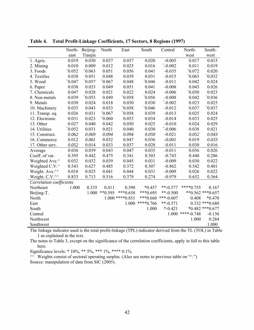
42

Table 4. Total Profit-Linkage Coefficients, 17 Sectors, 8 Regions (1997)

North-east

Beijing-Tianjin

North East South Central North-west

South-west

1. Agric. 0.019 0.030 0.037 0.037 0.020 -0.005 0.017 0.0152. Mining 0.010 0.009 0.012 0.025 0.016 +-0.002 0.011 0.0193. Foods +0.052 +0.063 0.051 0.056 0.041 -0.035 +0.072 0.0204. Textiles 0.038 0.051 0.048 0.039 0.031 -0.015 +0.063 +0.0325. Wood +0.047 +0.057 +0.067 0.048 +0.046 -0.011 0.042 0.0246. Paper 0.038 0.033 0.049 0.051 0.041 -0.008 0.043 0.0267. Chemicals 0.047 0.028 0.021 0.022 0.024 -0.006 +0.050 0.0238. Non-metals 0.039 +0.053 0.049 +0.058 +0.056 -0.008 0.042 +0.0369. Metals 0.030 0.024 0.018 0.030 0.030 +-0.002 0.023 0.02510. Machinery 0.035 0.043 0.033 +0.058 +0.046 -0.012 0.037 +0.03711. Transp. eq. 0.026 0.031 +0.067 +0.058 0.039 -0.013 0.025 0.02412. Electronic 0.031 0.023 +0.060 0.053 0.034 -0.014 0.033 0.02513. Other 0.027 0.040 0.042 0.050 0.025 -0.010 0.024 0.02914. Utilities +0.052 0.031 0.021 0.040 0.030 +-0.006 0.038 0.02115. Construct. 0.062 0.069 0.094 0.094 0.050 -0.021 0.052 0.04316. Commerce 0.012 0.061 0.032 0.047 0.036 -0.001 0.019 0.03317. Other serv. 0.052 0.014 0.033 0.037 0.028 -0.011 0.030 0.016Average 0.036 0.039 0.043 0.047 0.035 -0.011 0.036 0.026Coeff. of var. 0.395 0.442 0.475 0.341 0.303 -0.743 0.440 0.286Weighted Ave.^ 0.032 0.032 0.039 0.045 0.031 -0.009 0.030 0.022Weighted C.V.^ 0.543 0.627 0.485 0.372 0.307 -0.862 0.542 0.401Weight. Ave.^^ 0.018 0.025 0.041 0.044 0.031 -0.009 0.026 0.022Weight. C.V.^^ 0.833 0.713 0.516 0.379 0.274 -0.979 0.652 0.364Correlation coefficients Northeast 1.000 0.335 0.411 0.390 *0.457 **-0.577 ****0.755 0.167Beijing-T. 1.000 **0.595 ***0.658 ***0.695 **-0.500 **0.562 ***0.657North 1.000 ****0.851 ***0.660 ***-0.607 0.408 *0.470East 1.000 ****0.766 **-0.571 0.332 ***0.680South 1.000 *-0.421 *0.482 ***0.677Central 1.000 ****-0.748 -0.136Northwest 1.000 0.284Southwest 1.000The linkage indicator used is the total profit-linkage (TPL) indicator derived from the TL (TOL) in Table

1 as explained in the text. The notes to Table 3, except on the significance of the correlation coefficients, apply in full to this table

here. Significance levels: * 10%, ** 5%, *** 1%, **** 0.1%. ^^ Weights consist of sectoral operating surplus. (Also see notes to previous table on “^.”) Source: manipulation of data from SIC (2005).

43

Table 5. Correlation Coefficients Across 13 Industrial Sectors, Total Linkage Vs. State Share

Total output-linkage Total profit-linkage 1994 1997 2000 2003 1994 1997 2000 2003 Beijing *-0.481 -0.459 -0.415 *-0.505Tianjin **-0.644 -0.421 ***-0.717 -0.268Hebei **-0.642 ***-0.747 ***-0.690 ***-0.760 **-0.630 ***-0.768 **-0.682 ***-0.770Shanxi -0.016 -0.113 -0.124 0.024 -0.154 -0.082 0.072 0.020Neimenggu -0.335 *-0.526 -0.082 **-0.575Liaoning ***-0.713 -0.337 **-0.591 -0.368 *-0.516 -0.384Jilin -0.248 -0.295 -0.288 *-0.507 Heilongjiang -0.027 -0.079 -0.450 -0.375 -0.143 -0.022 -0.290 -0.261Shanghai -0.170 -0.248 -0.085 0.022 -0.099 -0.193 -0.040 0.039Jiangsu -0.259 -0.303 -0.149 -0.265 -0.336 -0.148Zhejiang -0.165 -0.263 -0.251 -0.167 -0.148 -0.242 -0.230 -0.152Anhui -0.112 -0.277 -0.315 -0.444 -0.066 -0.021 0.079 0.192Fujian -0.285 *-0.492 -0.317 -0.228 -0.221 -0.429 -0.310 -0.252Jiangxi -0.464 **-0.636 -0.313 0.161 0.248 0.219Shandong ***-0.697 ***-0.694 ***-0.697 ***-0.694 ***-0.701 **-0.689 ***-0.702 ***-0.701Henan *-0.475 *-0.476 -0.254 0.150 0.080 0.086Hubei -0.331 -0.291 -0.200 -0.242 0.026 0.042 0.080 0.179Hunan 0.045 -0.102 -0.097 -0.235 -0.123 -0.119Guangdong -0.218 -0.243 -0.168 -0.017 -0.124 -0.176 -0.175 -0.044Guangxi -0.326 -0.380 -0.245 -0.412 -0.373 -0.408 -0.159 -0.342Hainan 0.001 0.139 Chongqing -0.300 -0.400 -0.231 -0.353 -0.415 -0.335Sichuan -0.439 **-0.572 *-0.544 **-0.624 -0.375 *-0.475 **-0.521 **-0.647Guizhou -0.003 -0.177 -0.070 -0.143 -0.267 -0.236Yunnan -0.218 -0.431 -0.195 -0.379 **-0.635 -0.441Tibet Shaanxi -0.084 -0.025 -0.157 -0.139 -0.105 -0.094 -0.303 -0.309Gansu Qinghai *-0.508 -0.041 -0.401 **-0.559 -0.031 -0.333Ningxia Xinjiang -0.151 -0.161 0.334 -0.445 0.035 0.061 0.093 -0.124Northeast -0.244 **-0.569 -0.402 **-0.604 -0.179 -0.360 *-0.488 -0.308Beijing-T. *-0.481 **-0.644 -0.221 -0.415 ***-0.717 -0.224North ***-0.727 ***-0.718 **-0.687 ***-0.707 ***-0.729 ***-0.720 ***-0.690 ***-0.714East -0.240 -0.304 -0.031 -0.174 -0.241 -0.320 0.007 -0.164South -0.234 -0.330 -0.159 -0.036 -0.145 -0.265 -0.168 -0.062Central -0.344 -0.357 -0.135 -0.209 0.059 0.023 -0.048 -0.052Northwest -0.201 -0.219 -0.030 -0.397 -0.170 -0.209 -0.246 *-0.556Southwest -0.451 -0.405 -0.410 -0.414 -0.409 *-0.528 *-0.533 **-0.595The 13 sectors covered are the 13 industrial sectors (sectors 2 through 14) out of the total of 17 sectors. A province’s linkage coefficients across the 13 industrial sectors are those of the region in which the

province is located. State share denotes the state’s share in the output of all directly reporting industrial enterprises. Output is

value added except in the case of Shanghai, Jiangxi, and Qinghai, where only gross output value added data are available for all years (for Jiangxi in 2000 and Qinghai in 2000 and 2003, value added data would be available but gross output value data are used for consistency). Hubei 2003 also uses

44

gross output value data, because the sum sectoral SOSCE value added data significantly exceed the total for Hubei’s SOSCEs (only for 2000 would gross output value data also have been available; in years other than 2003, value added is used). For each province, output data on the 40 individual sectors are aggregated to match the 13 industrial sector aggregation in the 1997 regional input-output table.

An empty cell means that no data are available on the output either of the directly reporting industrial enterprises, or of the state-owned enterprises, or of both.

The “state” means SOEs in 1994 and 1997, and typically SOSCEs in the other years (with a very few exceptions, where the provincial statistics come according to the old SOE definition).

Significance levels: * 10%, ** 5%, *** 1%. For the regional coverage see note 17. Because linkage coefficients are regional values, combining these

with (aggregated) regional state shares, done in the bottom part of the table, yields the most meaningful correlation coefficients.

Sources: total linkage indicators calculated from SIC (2005) (or see Table 3 and Table 4); output data from provincial statistical yearbooks of the relevant years, supplemented with sectoral output data on the directly reporting industrial enterprises from the Industrial Yearbook in 1994 for Hebei, Shanghai, and Xinjiang, and in 1997 for Shanghai and Qinghai.

45

Table 6. Explaining Provincial Growth

I II III IV V VI VII VIII IX Constant ****11.05

(1.99)****12.58

(1.91)****10.44

(1.41)****4.76

(0.83) ****6.96

(1.40) ****5.69

(0.80)****7.59

(1.54)****4.62

(0.88)****7.02

(1.46)Dummy 1994-97 ****2.53

(0.43)***5.19

(1.55)***4.98

(1.62)****3.00

(0.50) ****7.04

(1.43) ****3.11

(0.58)****6.75

(1.58)****3.30

(0.59)****7.49

(1.48)Dummy 2000-03 ****1.50

(0.41)-1.18

(1.40)-0.76

(1.47)****1.61

(0.47) -0.88

(1.28) ***1.51

(0.54)-1.43

(1.43)***1.66

(0.54)-0.48

(1.36)Industrial sector variables TOL -3.10

(2.33)**-4.42

(2.03)

Coeff. of var. of TOL -1.55(4.37)

-0.72 (3.81)

TPL * dummy 1994-97 ****112.7 (26.0)

**64.36 (28.25)

90.13 (185.71)

272.16 (170.78)

TPL * dummy 1997-00 ****146.7 (25.7)

****118.95 (27.10)

*252.04 (150.04)

187.44 (136.15)

TPL * dummy 2000-03 ****147.0 (25.6)

****126.64 (28.91)

***190.82 (64.54)

***168.09 (58.26)

Coeff. of var. of TPL -10.74 (26.33)

29.95 (24.43)

-16.84 (30.59)

20.28 (28.47)

SOE share * dummy 1994-97 ****-7.47 (1.94)

****-7.26(1.98)

****-8.02 (1.74)

****-7.36 (1.85)

****-8.82 (1.87)

SOE share * dummy 1997-00 **-3.52 (1.62)

**-3.65(1.68)

*-2.52 (1.43)

-2.33 (1.54)

*-2.52 (1.46)

SOE share * dummy 2000-03 0.67 (1.57)

0.10(1.62)

1.07 (1.31)

2.04 (1.54)

0.59 (1.51)

Coeff. of var. of SOE share *6.80 (3.76)

4.85(3.72)

-1.47 (3.22)

1.34 (3.42)

-2.62 (3.40)

TPL-SOE * dummy 1994-97 ***81.71 (27.20)

42.52 (28.49)

21.51 (181.13)

-207.49 (164.92)

TPL-SOE * dummy 1997-00 ****121.36 (27.04)

****97.08 (27.62)

-105.27 (147.78)

-64.20 (129.00)

TPL-SOE * dummy 2000-03 ****118.22 (26.90)

***100.67 (29.71)

-37.60 (63.38)

-36.03 (62.35)

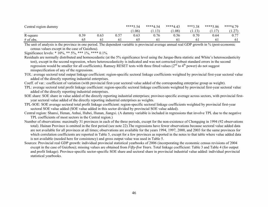
46

Central region dummy ****5.54 (1.06)

****4.54 (1.13)

****4.43 (1.08)

***3.38 (1.13)

****5.86 (1.17)

****4.79 (1.27)

R-square 0.39 0.63 0.57 0.63 0.76 0.56 0.70 0.64 0.77# of obs. 65 61 61 65 61 61 61 61 61The unit of analysis is the province in one period. The dependent variable is provincial average annual real GDP growth in % (post-economic

census values except in the case of Guizhou). Significance levels: * 10%, ** 5%, *** 1%, **** 0.1%. Residuals are normally distributed and homoscedastic (at the 5% significance level using the Jarque-Bera statistic and White’s heteroscedasticity

test), except in the second regression, where heteroscedasticity is indicated and was not corrected (robust standard errors in the second regression would be smaller for all coefficients). Ramsey RESET tests with three fitted values (2nd to 4th power) do not suggest misspecification of any of the regressions.

TOL: average sectoral total output linkage coefficient: region-specific sectoral linkage coefficients weighted by provincial first-year sectoral value added of the directly reporting industrial enterprises.

Coeff. of var.: coefficient of variation (with provincial first-year sectoral value added of the corresponding enterprise group as weight). TPL: average sectoral total profit linkage coefficient: region-specific sectoral linkage coefficients weighted by provincial first-year sectoral value

added of the directly reporting industrial enterprises. SOE share: SOE share in value added of the directly reporting industrial enterprises; province-specific average across sectors, with provincial first-

year sectoral value added of the directly reporting industrial enterprises as weights. TPL-SOE: SOE average sectoral total profit linkage coefficient: region-specific sectoral linkage coefficients weighted by provincial first-year

sectoral SOE value added (SOE value added in this sector divided by provincial SOE value added). Central region: Shanxi, Henan, Anhui, Hubei, Hunan, Jiangxi. (A dummy variable is included in regressions that involve TPL due to the negative

TPL coefficients of most sectors in the Central region.) Number of observations: maximally 31 provinces in each of the three periods, except for the non-existence of Chongqing in 1994 (92 observations

total). Hainan Province is omitted in the first period (see note 22).The regressions have fewer observations because sectoral value added data are not available for all provinces at all times; observations are available for the years 1994, 1997, 2000, and 2003 for the same provinces for which correlation coefficients are reported in Table 5, except for a few provinces as reported in the notes to that table where value added data is not available (needed here for consistency) and gross output value was used in Table 5.

Sources: Provincial real GDP growth: individual provincial statistical yearbooks of 2006 (incorporating the economic census revisions of 2004 except in the case of Guizhou); missing values are obtained from Fifty-five Years. Total linkage coefficient: Table 3 and Table 4 (for output and profit linkage). Province-specific sector-specific SOE share and sectoral share in provincial industrial value added: individual provincial statistical yearbooks.

47

Appendix A. Limitations to the interpretation of linkage coefficients and relevance to the

analysis in this paper

Beyond Hirschman’s caution towards the interpretation of quantitative measures of linkage

coefficients, a number of authors, including Diamond (1976), McGilvray (1977), Hewings

(1982), and Bulmer-Thomas (1982, section 12.5) raise further questions. First, in a less

developed country some sectors, perhaps especially those for which high linkages are expected,

may not yet exist. One solution would be to use the linkage coefficients of other—typically

developed—countries for which they are available. But Bulmer-Thomas questions if the

interdependence pattern found in less developed countries will eventually approximate that of

more developed countries. Another solution would be to simply assume values for the missing

input coefficients. The absence of precedents is less of a problem in the case of China in the

reform period, because at the beginning of the reform period a basic industrial structure was

already in place.

Second, an increase in gross output value is typically not a real world objective; an increase

in income is. But this is not an argument for discarding linkage indicators altogether. One way to

address the issue is to use income multipliers to turn output linkage indicators into income

linkage indicators, or employment multipliers to turn output linkage indicators into employment

measures. (For income, this is meaningful only if imports are non-competitive; if all imports are

competitive, a one-unit change in final demand necessarily implies a one-unit change in income,

value added, and the value of primary inputs).

The question of real world objectives is also a question of what weights, if any, to apply in

the derivation of sectoral linkage coefficients. (For example, in the case of the second backward

linkage indicator presented above, how to weight the Leontief inverse in the derivation of

sectoral linkage coefficients?) If one wants to avoid the assumption of a uniform one-unit final

demand change across all sectors, one can make each sector’s final demand change proportional

to the level of final demand in this sector. A further (or different) set of weights could be

desirable depending on policy objectives. Thus, the Leontief inverse could be pre-multiplied by a

48

diagonal policy matrix. However, policy objectives are likely to be multi-faceted and difficult to

quantify.

In this paper, linkage indicators are turned into profit-linkage coefficients in order to match

Hirschman’s exposition and to capture the likely mechanism through which linkage effects

operate in the economy. Whatever output change the government initiates, it is the impact on

profit opportunities that triggers new investment and thereby economic growth.

Third, choosing sectors by linkage ranking ignores efficiency or comparative costs. For

example, Riedel (1976) reports on sectors in Taiwan with low domestic linkage coefficients

which grew rapidly while intermediate inputs were imported. But this observation does not

contradict the linkage hypothesis in that (i) the linkage coefficient of a particular sector need not

have any implications for the growth rate of that particular sector, and (ii) Riedel does not

examine if import substitution occurs in the following years. This paper focuses on economy-

wide growth; it also allows the linkage coefficients of one year to be related to economic growth

several years later.

More generally, the input-output model assumes final demand to be exogenous. But a change

in final demand will trigger changes in primary inputs, which include household income, and a

change in household income will have an impact on final household demand. In order to

endogenize final household demand and primary inputs, a more elaborate social accounting

matrix framework is necessary. Given that the necessary data are not available for China, this is

not an option. Compared to the direct and indirect effects captured in the input-output table

framework, the induced effects via primary inputs are possibly minor. (If sectors are ranked by

the value of linkage coefficients, the induced effects via primary inputs may affect the ranking.

This happens if, for example, households’ marginal expenditure patterns differ from households’

average expenditure patterns. Such differences are likely, but if the induced effects are minor

they may not change the ranking of sectors.)

Fourth, ex ante linkage analysis comes with a severe flaw: current linkage indices need not

reflect future investment and growth opportunities that come into existence after new

49

government investment that potentially changes linkage coefficients.29 Linkage indices of more

developed countries could be applied, but this assumes that the country under examination will

go through an identical development process. Ex post linkage analysis appears more meaningful,

but carries no implications for the choice of development strategies and government investment

policies that reach into the future; at best, it can be used to evaluate government policies.30 This

paper provides an ex-post analysis to the extent that it examines the government’s allocation of

SOEs (after 1997) in response to linkage coefficients of different sectors and the ensuing effect

on economy-wide growth.

Fifth, sectors with high backward linkages, by definition, depend heavily on intermediate

goods, but these are often capital-intensive. The policy implications of favoring sectors with high

backward linkages would be to support capital-intensive industries, but “this is not a position to

which most LDCs [less developed countries] would want to be committed” (Bulmer-Thomas,

1982, p. 195). Hirschman (1984) addresses the issue implicitly when he argues that “once the

indirect employment effects (via backward and forward linkages) are taken into account,

investment in large-scale (capital-intensive) industry turns out to be just as employment-creating

as investment in small-scale (labor-intensive) industry for the industrially advanced countries of

Latin America” (p. 97). China’s government appears to have no scruples about promoting

capital-intensive industries, although some economic advisors (for example, Lin, 2003) promote

a more labor-intensive “comparative advantage following” development strategy for China.31

Sixth, the level of aggregation matters in the identification of high-linkage sectors. The level

of sectoral aggregation tends to be high, and inter-regional feedback mechanisms are typically

ignored. In the case of China, there is nothing that can be done about the level of aggregation,

given the data availability. However, a breakdown into 17 sectors is not trivial (given what the

literature on other developing countries can offer). As to inter-regional feedback mechanisms,

they may not be desirable (as explained in the section on linkage data above); China’s regional

data include intra-regional feedback effects in the provincial-level analysis.

50

Linkage indicators also come with technical limitations. Thus, input (or output) coefficients

are unlikely to be constant over time, whether due to technological change, economies of scale,

the invention of new products, substitution due to relative price changes, changes in consumer

preferences for the products within one sector, or changes from domestically produced to

imported inputs and vice-versa (for example, Miller and Blair, 1985, pp. 267f.). This concern is

alleviated by Yotopoulos and Nugent’s finding that the linkage coefficients for a number of

sectors are not significantly different between developing and developed countries; i.e., even as

China develops, changes in linkage coefficients are unlikely to be drastic, even over an extended

period. A second technical constraint is potential limits to available primary inputs, whether that

is labor or capital resources. Nevertheless, in a rapidly growing economy with widespread

underemployment in agriculture and a government-controlled banking system, resources do not

necessarily constitute an absolute constraint. If there is any scope for expansion, linkage

coefficients may indicate how to make the most out of limited resources.

51

Appendix B. Industrial sector data and state ownership

The data on industrial sectors and state ownership come with several statistical breaks. First, the

definition of SOEs changed in 1998 to include—in a new category of “state-owned and state-

controlled enterprises” (SOSCEs)—those SOEs which, by becoming a shareholding company

(possible since 1992/93), had escaped the pre-1998 definition of SOEs. Through 1997, “SOEs”

comprise the traditional state-owned enterprises, state-owned joint operation enterprises (a very

small category covering co-operations of two or more state-owned enterprises), and solely state-

invested limited liability companies. Since 1998, what is published are often data on the

aggregate of “state-owned and state-controlled enterprises” (SOSCEs) only. These comprise the

“SOEs” defined as previously and, furthermore, all other shareholding companies (i.e., all other

limited liability companies, plus all stock companies) in which the state has an absolute or

relative controlling share. The Company Law was passed in 1992 and enterprises only gradually

switched to the company system, which puts some limitation on the statistical break between the

SOE and SOSCE series in 1997-98.

In 1997, SOEs had value added of 919.293b yuan RMB. In 1998, SOSCEs had value added

of 1107.690b yuan RMB. I.e., value added of the state category (SOEs in 1997, SOSCEs in 1998)

grew by 20.5%. In comparison, industry-wide value added grew by 3.1% (8.9% in real terms).

The state share in the value added of the directly reporting industrial enterprises in 1997 was

46.3% and the SOSCE share in 1998 57.0%. (Statistical Yearbook 1998, p. 444; 1999, pp. 55, 57,

432)

The source of provincial industrial data by sector used here are the provincial statistical

yearbooks (the only publicly available source). Not all provinces immediately switched to the

new classification scheme in 1998. Even by 2000, half a dozen provinces still adhered to the

labels “SOEs” and “industrial enterprises with independent accounting systems at township level

and above” (see below). It could be that they still followed the old classification scheme, or that

they simply had not bothered to revise the terminology in their publications.

52

Second, the available data by industrial sector do not cover all industrial production units.

They only cover the “directly reporting industrial enterprises” (those that report regularly and

directly to China’s statistical authority). The definition of directly reporting industrial enterprises

changed in 1998.

Up through 1997, the directly reporting industrial enterprises comprise all enterprises with

independent accounting systems at township level and above (which include all SOEs), and since

1998 (though more gradually phased in at the provincial level) all state-owned and state-

controlled enterprises plus all non-state enterprises with independent accounting systems and

annual sales revenue in excess of 5m yuan RMB. The statistical break in the overall coverage of

the directly reporting industrial enterprises is on the order of a few percentage points: at the

national level, in 1997, the directly reporting industrial enterprises accounted for 62.5% of

industrial value added, and in 1998 (following the new definition), for 58.1%. The years

1997/1998 are a low point for the share of directly reporting industrial enterprises in industrial

value added. In 1994, the share was 80.1%. By 2007, the share had climbed from its all-time

1998 low of 58.1% to 105.9%. A value above 100% is logically impossible. (Statistical

Yearbook 1995, pp. 32, 388; 1998, pp. 55, 444; 1999, pp. 55, 433; 2009, pp. 37, 494. For a

discussion of this trend see Holz, 2008.)

A comparison of the sectoral data on the directly reporting industrial enterprises with the

industrial and economic census data of 1995 and 2004—both censuses covering a slightly larger

but still incomplete aggregate—shows that the production units not covered in the data on

directly reporting industrial enterprises are concentrated in sectors which, in the data on directly

reporting industrial enterprises, come with a low degree of state ownership (Holz, 2006). In other

words, if in a particular industrial sector the share of SOEs in the output of all directly reporting

industrial enterprises is low, then it is likely to be even lower (and possibly substantially lower)

in the (unknown) output of all production units in this industrial sector. On the other hand, if in a

particular industrial sector the share of SOEs in the output of all directly reporting industrial

enterprises is high, then it is likely to be the same or only minimally lower in the (unknown)

53

output of all production units in this industrial sector. Thus, in terms of the share of state

ownership in sectoral value added, the true share is likely to follow a more pronounced pattern

than the one found in the available data on the directly reporting industrial enterprises.

Third, the sectoral classification scheme was revised in 2003, but at the level of aggregation

used in the regional input-output table the changes appear minor. The 40 industrial sectors of the

earlier sectoral classification scheme can be seamlessly aggregated into the 13 industrial sectors

used in the 1997 multi-regional input-output table (following some explanations in the source,

SIC, 2005), and the 39 industrial sectors of the current sectoral classification scheme can be

matched well.

Fourth, beyond the period covered in the analysis here, the 2004 economic census unearthed

a number of enterprises with annual sales revenue in excess of 5m yuan RMB that had

previously managed to escape the reporting requirement. Industrial value added of 2004 was

revised up by 3.8% (Statistical Yearbook 2005, p. 51; 2006, p. 57). For the directly reporting

industrial enterprises and their sub-category of SOEs no revised 2004 data or revised data for

earlier years were published. If SOEs and non-SOEs among the directly reporting industrial

enterprises are equally affected by the revisions, then this statistical break does not affect the

share of SOEs in the directly reporting industrial enterprises in 2004 or earlier years, and

therefore has no implications for the analysis here. But they may also be unequally affected

because SOEs are supposedly all captured in the official statistics independent of their sales

revenue. Nevertheless, the size of the overall revision to industrial value added at 3.8% could be

small enough to ignore this statistical break. The group of directly reporting industrial enterprises

by nature changes every year as enterprises newly enter or exit this pool. In the year 2004, the

entry was probably slightly larger than in other years due to the special census efforts to capture

all relevant enterprises (with no possibility to revise the data of earlier years).

54

Notes 1 An earlier literature compares the production structures of different countries using input-output tables (for example, Chenery and Watanabe, 1958) without exploring the unbalanced growth hypothesis 2 Further, Wade (2009, pp. 352ff.) views industrial policy as “any sectorally or activity-targeted interventions” and distinguishes between government leadership of the market (leading decentralized private producers to do something they would otherwise not do) and government followership of the market (betting on some of what the private sector is already doing); the unbalanced growth hypothesis suggests government leadership, including in form of government-organized production. Pack and Saggi (2006, pp. 267f.) define industrial policy as “any type of selective government intervention or policy that attempts to alter the structure of production in favor of sectors that are expected to offer better prospects for economic growth in a way that would not occur in the absence of such intervention in the market equilibrium.” This definition, too, includes the unbalanced growth hypothesis. 3 For sector-specific industrial policy studies in the case of China (electronics manufacturing, aircraft manufacturing, and steel) see Zhao et al. (2007), Goldstein (2006), and Sun (2005). 4 For an overview of the ownership transition see Naughton (1996; 2007, Chapter 13). 5 Recent quantitative analyses of privatization appear to not control for such factors as the government-financed reductions in social burdens, the debt write-offs, and the restructuring that inevitably accompany privatization. I.e., the performance of newly privatized firms may improve due to reasons other than privatization. While much of the discussion of SOEs has focused on profitability, there is also a literature on efficiency; it typically concludes on the inferiority of SOEs (see, for ex., Jefferson et al., 2000). 6 A discussion of Yotoupolos and Nugent’s (1973) paper in a later issue of the Quarterly Journal of Economics by Laumas (1976), Boucher (1976), Riedel (1976), and Jones (1976) provides a number of arguments which Yotoupolos and Nugent (1976) defend themselves against. Thus, sectors are weighted in their original analysis, imports are excluded in the calculation of their linkage coefficients, other linkage indicators are highly correlated with theirs, and the level of aggregation was dictated by the data. 7 There is likely also a discrepancy in how linkage effects and growth rates are measured. The linkage index measures the impact of one unit change in final demand of one particular sector on gross output value across the economy. Growth rates are presumably measured in terms of value added. (The authors do not clarify.) 8 The division in that formula by the number of sectors (to average across sectors) in their equation appears redundant given that the weights (applied to the squared sectoral deviations from the linkage-weighted economy-wide growth rate) consist of the share of each sector in GDP. 9 An earlier article by Yotopoulos and Lau (1970) examines the relationship of imbalance and growth without reference to linkages; it concludes in favor of balanced growth. (The authors defend their measure of imbalance in 1975.) 10 These include Bhalla and Ma (1990) with a comparison of China’s 1981 linkage coefficients to those in other countries and a focus on agricultural vs. rural non-farm vs. light industry vs. heavy industry linkages, Heimler (1991) with sectoral indices of vertical integration for 1981, Li and Xue (1998) with sectoral linkage coefficients for 1981, 1983, 1987, 1990, 1992, and 1995 (using constant-price input-output tables), Liu (2003) with sectoral linkage coefficients for 1997, and Andreosso-O’Callaghan and Yue (2004) with an examination of the development of a range of sectoral linkage coefficients between 1987 and 1997. Input-output literature for China that does not focus on linkage effects includes an examination of structural change over time (Coady and Jie, 1993, for 1981, 1983 and 1987 using a proportional column filter and Andreosso-O’Callaghan and Yue, 2004, for 1987 and 1995 using a biproportional filter) and a decomposition of output growth into changes of final demand level, final demand structure, technical coefficients, and exports (Andreosso-O’Callaghan and Yue, 2002). Ichimura and Wang (2003) examine China’s interregional dependence based on 7 regions and 9 sectors. Xu and Liu (2004) contain a large collection of short articles related to input-output analysis. Li (1992) is a textbook on input-output table techniques. Polenske and Chen (1991) present a historical overview over input-output tables in China as well as numerous applications that provide evidence of extensive applied input-output work in China. 11 This may be clearer if the Leontief inverse is rewritten as (I-A)-1 = (I + A + A2 + A3 + …); writing out A2, A3 etc. reveals the forward linkage input coefficients. Backward and forward linkage indicators both share the intra-sectoral flows, i.e., the intra-sectoral flows are double-counted. Diamond (1976) suggests two possible adjustments to the Leontief inverse, namely to subtract out the initial one-unit increase in the final demand for the particular sector under consideration, and to further omit the intra-industry effects in this sector. The first adjustment should not affect the ranking of sectors by linkage coefficient because each sector under consideration contains the initial one-unit increase in final demand. 12 Cai and Leung’s work builds on a long line of literature on the extraction method, originating with Strassert (1968) and Schultz (1977). Cella (1984) then decomposes the total linkage coefficient into backward and forward linkages (with backward linkages, however, including some forward elements, and vice versa). Among the subsequent literature, Clements (1990) provides an adjustment to Cella’s split of the total linkage indicator into

55

backward and forward linkage, which also implies a different normalization. Sonis et al. (1995) introduce the concept of pure linkages that further disentangles the backward and forward linkages (Cai and Leung interpret Sonis’ pure linkages and suggest their alternatives). Dietzenbacher and Linden (1997) propose an approach that allows for a natural distinction of the interdependencies into backward and forward linkages. 13 A number of other total linkage indicators are possible and presented by Miller and Lahr (2001). Cella (1984) includes the output effect in the omitted sector in his total linkage effect; the part of his formula that covers the non-extracted sector is identical to the formula used here. While government activity in one sector may trigger non-government activity in the same sector, the two cannot be distinguished. Therefore, it seems more appropriate to examine the impact of the extracted sector on the non-extracted sectors. 14 See, for example, Jones (1976, p. 329). For the linkage coefficients calculated from the columns of the Leontief inverse or Gosh inverse, Jones shows that the sum of sectoral BL(2)s weighted by the (sectoral) value of output equals the sum of sectoral FL(2)s weighted by the (sectoral) value of output; i.e., the output-weighted sum of sectoral BL(2)s or FL(2)s equally yields the coefficient of interdependence. In order to determine a relative degree of sectoral linkage, one option is to standardize by the average degree of linkage across the economy (linkage coefficient of a particular sector divided by average linkage coefficient across all sectors). Another option, if data on several geographic entities with identical sectoral classification are available, is to standardize by the average degree of linkage in the particular sector across geographic entities. Standardization is not needed below. 15 For a discussion of the term “operating surplus” in the National Income and Product Accounts vs. the accounting term “ profit,” in the case of China’s industry, see Holz (2003). 16 Naughton (2003) believes that provincial input-output tables should exist, in accordance with the 5-year frequency, for 1982, 1987, 1992, 1997, and 2002. A national input-output table was possibly compiled also for 1973. 17 The eight regions are Northeast (Heilongjiang, Jilin, Liaoning), Beijing-Tianjin, North (Hebei, Shandong), East (Jiangsu, Shanghai, Zhejiang), South (Fujian, Guangdong, Hainan), Central (Shanxi, Henan, Anhui, Hubei, Hunan, Jiangxi), Northwest (Inner Mongolia, Shaanxi, Ningxia, Gansu, Qinghai, Xinjian), and Southwest (Sichuan, Chongqing, Guangxi, Yunnan, Guizhou, Tibet). The 17 sectors are listed in Table 3. The sectors in the 1987 inter-regional input-output table (not used here) are agriculture, mining and processing, light industry, energy industry, heavy industry and chemical industry, construction, transportation & post & telecommunications, commerce and catering, and “non-material” sectors (Ichimura and Wang, 2003, p. 14). 18 Because domestic trade flows are not particularly large, the necessary choice between local vs. national planning is unlikely to be important. Across the eight regions in 1997, for intermediate use between 8-13% of GOV was domestically imported, while between 6-14% of final demand was. (These numbers, 8% etc., reflect an individual region’s aggregate across sectors; the percentages differ further for each sector in a region.) On the domestic export side, between 8-21% of domestic gross output value of a region’s intermediate sales went to other regions, and between 3-11 % of final demand. (Again, 8% etc. reflect a region’s aggregate value.) 19 The central government, under the State-owned Asset Supervision and Administration Commission, retains only a few large holding companies (196 in 2003, merged to 116 in 2009). For the transfer of centrally owned coal mines to provinces in 1998 see, for example, Su (2004). Regarding investment, local investment (independent of ownership form) in 1997 was more than twice the size of central investment, and in 2008 eight times (Statistical Yearbook 2009, p. 181). For some years, SOE-specific data are available; in 1997, local SOE investment was 1.5 times central SOE investment (Investment Yearbook 1998, p. 52). Whatever investment occurs in centrally owned SOEs is furthermore likely to be at least partially influenced by local government policy. 20 International imports could be made non-competitive by assuming each sector’s international imports to occur in some specific proportion across sectors (and non-import final demand) to which they are directed; but it is doubtful if such proportionality assumptions are plausible. International imports accounted for the following percentages of regional final demand (where final demand includes international imports): 9 (Northeast), 36 (Beijing-Tianjin), 7 (North), 20 (East), 31 (South), 3 (Central), 5 (Northwest), 2 (Southwest). 21 In the case of the INT and GSD, the Central region’s sectoral pattern of profit linkage coefficients is positively correlated with those in other regions. 22 Throughout all regressions reported in this section, Hainan Province is omitted in the first period (1994-97). If included, its residual constitutes a far outlier that can significantly influence the regression coefficients. The outlier status originates in an unusually low provincial real growth rate of value added with an average annual 5.1% in the first period. These values contrast with 41%, 21%, and 11% annual real growth rates in 1992 through 1994. 23 A coefficient of variation of TPL-SOE is not included because its interpretation appears not straightforward. If included, its coefficient tends to be insignificant except in the third period, when it tends to be negative and significant. (This is independent of if the squared term in the standard deviation is weighted by the SOE share or not.) Inclusion of the coefficient of variation has only a very minor impact on the coefficients of the other variables.

56

24 One might want to argue that a particular degree of imbalance in the state share, matching in some way the sectoral distribution of linkage values, is optimal for economic growth. But including the coefficient of variation of the state share in linear and squared form in the regressions also yields insignificant coefficients. 25 In these regressions, all 92 observations (31 provinces, of which Chongqing only came into existence in the second period), less Hainan Province in the first period, can be used, whereas the regressions reported in Table 6 are restricted to those combinations of provinces and time periods for which industrial SOE (or directly reporting industrial enterprise) value added data are available. TOL and TPL involve sectoral weights (that, at the provincial level, require the use of value added data for the directly reporting industrial enterprises); similarly, in the calculation of the standard deviation (used in the derivation of the coefficient of variation of TOL or TPL) the squared deviations from the mean are weighted by sectoral value added. Not applying sectoral value added weights when aggregating sectoral TL coefficients to an economy-wide regional TL value makes no qualitative difference to the results. 26 The necessary deflators are national sectoral deflators derived from nominal and real gross output values in the 37-40 industrial sectors, except in 2003 when, lacking real gross output value data, the ex-factory price index is used. (The NBS’s procedure for deriving the industrial real growth rate of value added closely matches the procedure chosen here; see Holz, 2006.) Data sources are the annual Industrial Statistical Yearbook and the annual Statistical Yearbook series. 27 Experimenting with the inclusion of a variable measuring capital growth (based on the original value of fixed assets deflated in full at the current year’s investment prices), the variable tends to be insignificant or barely significant (with a positive sign). 28 See http://www.ndrc.gov.cn/fzgh/ghwb/gjjh/P020070912638573307712.pdf, accessed April 2010. 29 A counter-example is the potential for import substitution revealed by the difference between an intermediate input coefficient matrix that incorporates vs. excludes imports. 30 Bulmer-Thomas (1982, p. 196) sees a role for ex post linkage analysis to (i) check if government policy, at a given point in time, is consistent with the ranking of sectors, (ii) identify ‘enclave’ sectors (which could trigger policies to integrate these into the national economy), (iii) track changes in the sectoral interdependence of a country over time, and (iv) make international comparisons at a given point in time. 31 A high degree of labor intensity necessarily implies low linkage coefficients. Social accounting matrices, in contrast to input-output tables, would take into account the use of the relatively large newly created income of laborers when investment occurs in high labor-intensity low-linkage sectors.