Forthcoming in Recovery Risk: The Next Challenge in Credit Risk Management, editors E. Altman, A. Resti and A. Sironi, Risk Books.

HOW TO MEASURE RECOVERIES AND PROVISIONS ON BANK LENDING

Methodology and Empirical Evidence

J. Dermine and C. Neto de Carvalho* Third draft: 28 March 2005

INSEAD (Fontainebleau) and Universidade Catolica Portuguesa (Lisbon), respectively. The authors are grateful to A. Resti, P. Jackson, M. Massa, J. Santos Silva, A. Sironi, M. Suominen, and J. Wahlen for helpful discussion, to J. Cropper for editorial assistance, and to

1Banco Comercial PortuguLs for access to internal credit data.

Introduction

The purpose of this chapter is to propose a methodology to estimate losses-given-default (LGD)

and fair provisions on non-performing bank loans. The methodology is then applied to a unique set

of micro-data on loans to small- and medium size enterprises (SMEs). LGD estimates are important

inputs in the pricing of credit risk, and measurement of bank profitability and solvency. The

international bank capital regulations, Basel II, require estimates of losses-given-default to calculate

risk-weighted assets, and to estimate the fair level of provisions needed to adjust the amount of

available capital.1

The chapter is structured as follows. In Section 1, we argue that bank loans are likely to have some

characteristics significantly different from those of corporate bonds. This justifies the need for

specific studies on bank loans. In Section 2, the database on individual loans losses is presented.

The mortality-based approach to analyze recovery rates on bad and doubtful loans is discussed in

Section 3. Empirical evidence on cumulative recovery rates is presented in Section 4. In Section 5,

we show how to use the methodology to calculate dynamic provisions over time. In Section 6, a

multivariate statistical analysis of the determinants of loan losses-given-default and provisions is

developed. Section 7 concludes the chapter.

Section 1. LGD Literature Review

If several authors have analyzed credit risk and losses-given-default on corporate bonds, few

1 Under the Basel II internal rating-based (IRB) approach, two cases must be distinguished: Estimates of losses-given-default are needed for the retail loan portfolio under the ‘foundation’ approach, while LGD on corporate loans are needed only for the ‘advanced’ approach. Banks using the IRB approach must compare their total eligible provisions with the total expected losses (Basel Committee, 2004).

2studies have been applied to bank loans. The reason for this is that, as bank loans are private

instruments, few data are publicly available.

The seminal work by Altman (1989) on US corporate bonds defaults was followed by studies on

recovery rates, and on the degree of correlation between default frequencies and recovery rates

(Frye 2000a,b and 2003, Altman et al., 2003, or Acharya et al., 2003). These studies relied on

publicly traded bond data. In view of this literature, one needs to justify a study on recovery on bank

loans. Several arguments are proposed. The first two are that small firms are informationally more

opaque, and that the relationship between the owner/manager of the firm and the bank is often very

close (Allen et al., 2004). This has two implications. In the case of distress, the owner/manager has

relatively more to lose because his or her skills will be firm-specific. Effort to repay a loan could be

greater than in large public firms. Second, the close relationship with a bank might imply that the

latter will hesitate to foreclose a loan, hoping to capture the option value of a future relationship

(Dewenter and Hess, 2004). A third argument is that a bank might hesitate to foreclose large loans,

if it believes that this can have local spillover effects on other firms, i.e., clients of the bank. In the

arm’s-length transactional corporate bonds markets, these ‘option’ or ‘macro’ considerations will

be ignored. A fourth reason is that a large number of distressed loans may create bottlenecks in the

workout unit of the bank, with effect on recovery rates. Finally, in the case of distressed bank loans,

knowledge of the timing of cash flow recoveries will be useful to measure interest rate risk, with

computation of repricing gaps or duration measure, as well as to provide information to calculate

dynamic loan loss provisions over time.

As mentioned above, few studies have focused on the bank loan markets because of the private

nature of these transactions. Asarnow and Edwards (1995) examined 831 defaulted loans at

Citibank over the period 1970-1993. They reported an average cumulative recovery rate of 65%.

Carty and Lieberman (1996) measured the recovery rate on a sample of 58 bank loans. Based on

secondary market prices for defaulted bank loans for the period 1989-1996, they reported an

average defaulted bank loan price of 71%. The above studies focused on the US market. Hurt and

Felsovalyi (1998) analyzed 1,149 bank loan losses in Latin America over the period 1970-1996.

They report an average recovery rate of 68.2 % and show that loan size is a contributory factor to

loss rates, with large loan default exhibiting lower recovery rates. They attribute this to the fact that

3large loans, often not secured, are made to economic groups that are family owned.2 None of the

above studies provide information on the timing of recoveries.

Thanks to access to a unique data-base on loans to SMEs, this chapter provides empirical evidence

on the timing of recovery on individual bad and doubtful loans, on cumulative recovery rates, and

their economic determinants.

Section 2. Bank Loan Losses, Database and Measurement Issue

The database was provided by the largest private bank in Portugal, Banco Comercial Português

(BCP). It consists of 374 non-performing loans granted to SMEs over the period June 1995 to

December 2000.

Table 1 (Panels A and B) provides information3 on the number of defaults per year, and the

amount of debt outstanding at the time of default. Table 1 (Panels C and D) shows the number of

loans with guarantee or collateral, the age of the firm, and the number of years of relationship with

the bank. One observes that the series of 374 default cases is distributed evenly over the six –year

period, and that the distribution of debt outstanding at the time of default is highly skewed toward

the low end. The available information in the database includes the history of the loan after a default

has been identified, the type of collateral or guarantees, the industry classification, the interest rate

charged on the loan, the internal rating attributed by the bank, the age of the firm, and the length of

relationship with the bank.

In Table 1 (Panel C), the various forms of guarantees or collateral are reported. These include:

! Guarantees

! Real estate collateral

! Physical collateral (inventories)

! Financial collateral (bank deposits, bonds or shares)

2 An additional study includes La Porta, Lopez-de-Silanes and Zamarripa (2003), who analyze loan default and losses-given-default in Mexico in the context of ‘related lending’, that is, lending to shareholders or directors of the bank. 3 The data gathered for this study do not include any reference to the identity of the clients or any other information which, according to Portuguese banking law, cannot be disclosed. A more complete description of

4Insert Table 1

In 35.6% of the cases, there is no guarantee or collateral. Guarantees, which are used in 58.3% of

the cases, refer to written promises made by the guarantor (often the owner or the firm’s director)

that allows the bank to collect the debt against the personal assets pledged by the guarantor.

Collateral is used in 15% of the cases.

Panel D of Table 1 shows the age of the firm, and the number of years of relationship with the bank.

Companies have, on average, a life of 17 years, with extremes going from 6 months to 121 years.

The average relationship with the bank is six years.4

Any empirical study of credit risk raises two measurement issues. Which criterion should be used to

define the time of a default event? Which method should be used to measure the recovery rate on a

defaulted transaction?

The criterion used for the classification of a loan in the ‘default’ category is critical for a study on

recovery rates, as a different classification would lead to different results. Three ‘default’ definitions

are used in the literature:

i) A loan is classified as ‘doubtful’ as soon as “full payment appears to be questionable on the basis

of the available information”.

ii) A loan is classified as ‘in distress’ as soon as a payment (interest and/or principal) has been

missed.

iii) A loan is classified as ‘in default’ when a formal restructuring process or

bankruptcy procedure is started.

In this study, because of data availability, we adopt the second definition, that is, a loan is classified

as ‘in default’ as soon as a payment is missed.5

the database is available in Dermine and Neto de Carvalho (2005). 4 The relatively short average relationship is due to the fact that the bank was created in 1985, after the deregulation of the Portuguese banking system. 5 For the sake of comparison, the definition of default adopted by the Basel Committee is as follows (Basel Committee, 2004, p. 92): “A default is considered to have occurred with regard to a particular obligor when either or both of the two following events have taken place: a) The bank considers that the obligor is unlikely to pay its credit obligations to the banking group in full, without recourse by the bank to actions such as realizing security (if held).

5

The second methodological issue relates to the measurement of recovery on defaulted loans. There

are two methodologies:

i) The price of the loan at the default date, defined most frequently as the trading price one month

after the default. This approach has been used in studies on recoveries on corporate bond defaults.

ii) The discounted value of future cash flows recovered after the default date.

As no market price data are readily available for defaulted bank loans in Portugal, the second

methodology -the present value of actual recovered cash flows- is the only feasible alternative. This

approach was adopted by Asarnow and Edwards (1995), Carty and Lieberman (1996), Hurt and

Felsovalyi (1998), and La Porta et al. (2003). The present value of cash flows recovered on

impaired loans allows us to measure the proportion of principal and interest that is recovered after

the default date. This approach has the advantage that, if the loan is fully repaid, the present value of

the actual cash flows recovered will be equal to the outstanding balance at the default date. It should

be noted that this PV amount could differ from the price of the loan at a time of default, which would

incorporate the expected cash flows and proper risk or liquidity premia.

Two approaches will be used to analyze the recovery rates, a univariate mortality-based approach,

and a multivariate statistical analysis of the determinants of recovery.

Section 3. A Mortality-based Approach to Analyze Recovery Rates

Having access to the history of cash flows on these loans after default, we can study the time

distribution of recovery. With reference to the studies by Altman (1989) and Altman and Suggitt

(2000), we apply the mortality approach. It must be noted that the mortality approach was applied

to measure the percentage of bonds or loans that defaulted n years after origination. The application

of mortality to loan recovery rates is, to the best of our knowledge, novel. It examines the

percentage of a bad and doubtful loan which is recovered n months after the default date. This

b) The obligor is past due more than 90 days on any material credit obligation to the banking group. Overdrafts will be considered as being past due once the customer has breached an advised limit or been advised of a limit smaller than current outstandings”.

6methodology is appropriate because the population sample is changing over time. For some default

loans, i.e., those of June 1995, we have a long recovery history (66 months), while for the recent

‘2000’ loans in default, we have an incomplete history of recovery.

To define the concepts used to measure loan recovery rate and provisions on impaired loans6, it is,

for expository reasons, useful to refer to a simple example. Formal definitions of concepts are

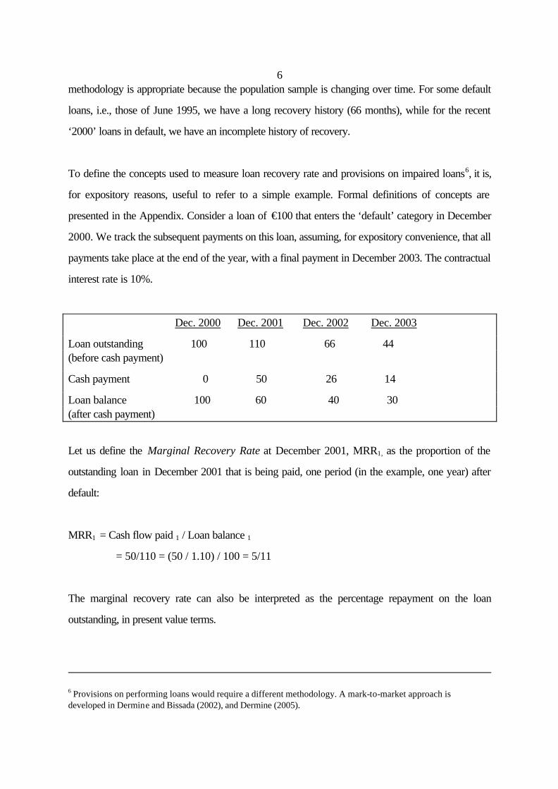
presented in the Appendix. Consider a loan of €100 that enters the ‘default’ category in December

2000. We track the subsequent payments on this loan, assuming, for expository convenience, that all

payments take place at the end of the year, with a final payment in December 2003. The contractual

interest rate is 10%.

Dec. 2000 Dec. 2001 Dec. 2002 Dec. 2003

Loan outstanding 100 110 66 44 (before cash payment)

Cash payment 0 50 26 14

Loan balance 100 60 40 30 (after cash payment)

Let us define the Marginal Recovery Rate at December 2001, MRR1, as the proportion of the

outstanding loan in December 2001 that is being paid, one period (in the example, one year) after

default:

MRR1 = Cash flow paid 1 / Loan balance 1

= 50/110 = (50 / 1.10) / 100 = 5/11

The marginal recovery rate can also be interpreted as the percentage repayment on the loan

outstanding, in present value terms.

6 Provisions on performing loans would require a different methodology. A mark-to-market approach is developed in Dermine and Bissada (2002), and Dermine (2005).

7Let us define the Percentage Unpaid Loan Balance after payment in December 2001, PULB1, as

the proportion of the December 2001 loan balance that remains to be paid one period after default :

PULB1 = 1 – MRR1 = 1 – 5/11 = 6 /11

One can define the Marginal Recovery Rate and the Percentage Unpaid Loan Balance at

December 2002, two periods after default:

MRR2 = Cash flow paid 2 / Loan 2 = 26/66

PULB 2 = 1 – MRR2 = 1 – 26/66 = 40/66

And, the Cumulative Recovery Rate in December 2002 for a loan defaulting in December 2000,

CRR0,2 , is defined as:

CRR 0,2 = 1 – (PULB1 x PULB2)

= 1 – (6/11 x 40/66) = 1 – 240/726 = (1 – 40/121) = 81/121

= (81/1.12) /100 = 66.9%

Similarly, one can calculate a Marginal Recovery Rate, MRR3, a Percentage Unpaid Loan

Balance, PULB3, and a Cumulative Recovery Rate, CRR0,3, at December 2003 =

MRR3 = Cash flow paid 3 / Loan 3

= 14/44

PULB3 = 1 – MRR3 = 1 – 14/44 = 30/44

CRR 0,3 = (1 – (PULB1 x PULB2 x PULB3)

= 1 – (6/11 x 40/66 x 30/44) = 1 – 7,200 / 31,944 = 1 – 30/133.1

= 103.1/133.1 = (103.1/1.13) / 100 = 77.5%

Similar to Carey (1998), Asarnow and Edwards (1995), Carty and Lieberman (1996), Hurt and

Felsovalyi (1998), and La Porta et al. (2003), the Cumulative Recovery Rate at time T on a loan

8balance outstanding at time 0, CRR0,T, represents the proportion of the initial defaulted loan that has

been repaid7 (in present value terms), T periods after default.

Finally, the Loan-Loss Provision, LLP0, on a loan balance outstanding at the default date,

December 2000, is defined as:

LLP0 = 1 - CRR 0,3 = 1 - 0.775 = 22.5% .

This percentage, 22.5%, represents the percentage of the loan that will not be recovered

(interest included) in the future. With perfect foresight, it would serve as a base for provisioning on

the loan at the time of default.

A related question is to analyze the provision on a loan, n years after the default date. This allows

the calculation of dynamic provisions. Moving forward, one can define a Cumulative Recovery

Rate, CRR 1,3 , on a loan balance outstanding at December 2001, and a dynamic Loan-Loss

Provision, LLP1, on a loan balance outstanding at December 2001. These are defined as :

CRR 1,3 = (1 – PULB2x PULB3) = 1 - 40/66 x 30/44 = 58.7%

LLP1 = 1 – CRR1,3 = 41.3%

In a similar manner, the Cumulative Recovery Rate, CRR2,3, and the dynamic Loan-Loss

Provision, LLP2, on a loan balance outstanding at December 2002 are defined as :

CRR 2,3 = (1 – PULB3) = 1 - 30/44 = 31.8%

LLP2 = 1 – CRR2,3 = 68.2%

Knowledge of marginal recovery rates over time thus allows one to calculate the dynamic evolution

of provisions over time.

Having computed the cumulative recovery rate on individual loans, one can compute an arithmetic

average cumulative recovery rate for the sample of loans. Alternatively, one can compute a

principal-weighted average recovery rate that will take into account the size of each loan. A

7 One observe that 103.1, in CRR0,3, is the future capitalized value of interim cash flow recovered (103.1 = (50x1.12 ) + (26x1.1) + 14).

9comparison of the sample weighted cumulative recovery rate with the average of recovery rates on

individual loans will be indicative of a size effect.

Section 4. Cumulative Recovery Rates, Empirical Results

The sample marginal and cumulative recovery rates for the sample T periods after a default date,

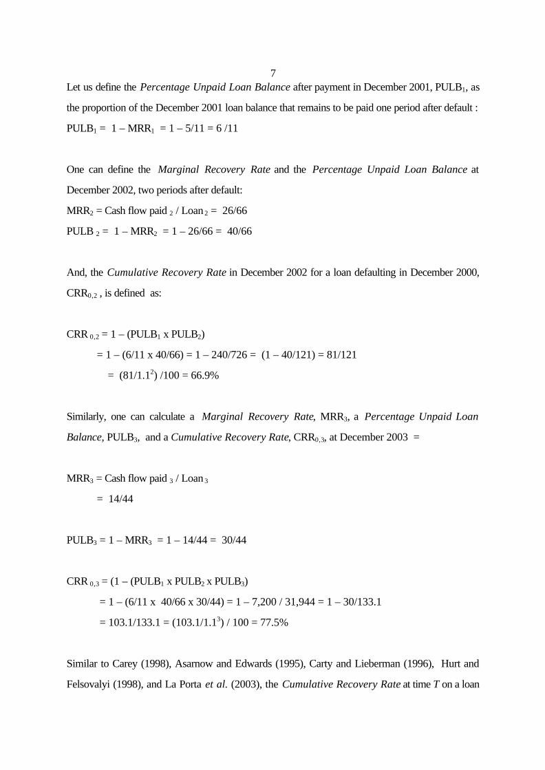
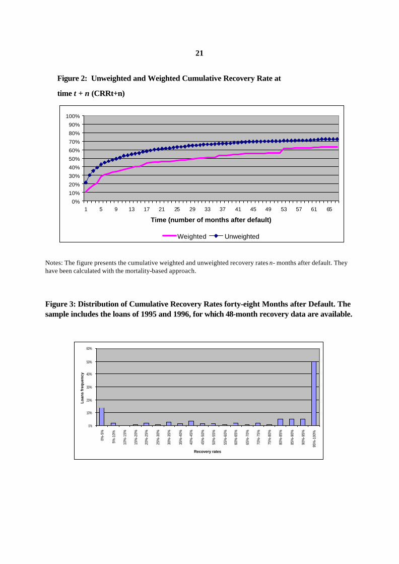
SMRRT and SCRRT , respectively, are reproduced in Figures 1 and 2.

Insert Figures 1 and 2

In Figure 1, one observes that most of the marginal recovery rates in excess of 5% occur in the first

five months after the default, and that the cumulative average recovery rate is almost completed after

48 months. As indicated in Figure 2, the unweighted (weighted) cumulative recovery rates8 after 36

and 48 months are, respectively, 67.3% (53.5%) and 70% (56.3%). The differences between the

unweighted and weighted average cumulative recovery rates are an indicator that recovery on large

loans is significantly lower.

It is also of interest to analyze the distribution of cumulative recovery rates across the sample of

loans. The distribution of cumulative recovery rates after 48 months is reproduced in Figure 3. This

figure shows a bi-modal distribution with many observations with low recovery, and many with

complete recovery. These results are quite similar to those reported by Asarnow and Edwards

(1995) and Schuermann (2004) for the US, and Hurt and Felsovalyi (1998) for Latin America.

Loan portfolio models which incorporate a probability distribution for recovery rates should take

into account this bi-modal distribution.9

Insert Figure 3

Section 5 . Loan-Loss Provisioning, Empirical Evidence with a Mortality-

8 Note that, as is the case of other studies, these are gross recovery rates. Estimates of the bank’s internal recovery costs, which include the cost of the workout units and legal and accounting costs, are discussed in Dermine and Neto de Carvalho (2005). 9 Current commercial credit portfolio models do not incorporate the bi-modal distribution. For instance, CreditRisk+ assumes a fixed expected recovery rate within each band, while CreditMetrics uses a beta distribution (Crouhy et al., 2000).

10based Approach

The accounting and finance literatures have analyzed three main provisioning issues related to private

information held by banks on loans: the extent of earnings and capital smoothing (Hasan and Wall,

2004), the impact of reported provisions on a bank’s stock returns (Wahlen, 1994), and the

systemic impact on the banking industry of disclosure on loan provisions by one bank (Grammatikos

and Saunders, 1990). These studies are concerned with fair level of provision at the portfolio level.

To the best of our knowledge, none have dealt with provisions at the micro level. As defined in

Section 3, loan-loss provision is the complement of the cumulative recovery rate.

Insert Table 2

Cumulative recovery on outstanding balances on bad and doubtful loans are reported in Table 2.

These dynamic cumulative recoveries are calculated on loan balances outstanding n months after the

default date, with n varying from 0, the time of financial distress, to 37 months after the default date.

Over time, the weighted (and unweighted) cumulative recovery rates on the unpaid loan balance are

decreasing monotonously over time, 63.8% (72.6%) in month 0, to 23.3% (17.1%) in month 37.

More complete information is obtained (Table 2), by dividing the sample into three groups,

according to the absence of guarantee/collateral, the existence of guarantee, or the existence of

collateral support. As expected, the cumulative recovery rates (unweighted, so as not to be

affected by the size effect) is the highest for the case of loans with collateral for every period, for

instance 85.3% at time 0, the default date. A counterintuitive and significant observation is that the

(unweighted) cumulative recovery rates on loans without any type of guarantee or collateral

dominates, in every period, the cumulative recovery rate on loans with guarantees. For instance, at

time 0, (unweighted) recoveries on loans without any type of guarantee/collateral is 80.6%,

vs.63.9% for recoveries on loans with guarantee (or 47.0% vs. 20.8%, 19 months after the default

date). This result is likely to be due to two factors. First, as explained by the bank, guarantee or

collateral support is not usually requested from reliable clients, so that the existence of a guarantee is

an indicator of greater risk. Second, some borrowers are able to shift ownership of personal

assets to other persons, so that, when the bank tries to execute the debt, there is not much left. This

empirical result, if confirmed in other studies, implies that regulatory provisions should not necessarily

penalize loans without guarantee, as the absence of a guarantee might be justified by higher expected

recoveries.

11

Section 6. Loan-Loss Provisioning, a Multivariate Analysis

In the previous sections, univariate mortality-based estimates of cumulative recoveries and

provisions were provided. In this section, we attempt to estimate empirically the determinants of the

cumulative recovery rates and dynamic provisions. A discussion of the choice of explanatory

variables and the econometric specification is followed by the empirical results.

Explanatory variables and econometric specification

Explanatory variables include the size of the loan, the type of guarantee/collateral support, past

cumulative recovery, the age of the firm, and the industry sector. Fifteen business sectors have been

created, with reference to the European Union’s NACE economic activity codes. Further

aggregation, used in the econometric tests, leads to four activity sectors: real sector (activities with

well identified real assets, such as land, mines or real estate property, which could be used for

security), manufacturing, trade, and services. The size of the loan is included because some

empirical studies and the sample univariate weighted and unweighted average cumulative recovery

data have pointed out the effect of the loan size. Past cumulative collection is included on the

assumption that a good level of collection could indicate a genuine effort by the borrower to repay

the loan fully. A year dummy is included so as to have a better understanding of the volatility of the

recovery rate over time. Finally, it is of interest to know the impact of guarantee/collateral, as, if

statistically significant, this variable will be taken into account in calculating loan-loss provisions on

bad and doubtful loans.10

The size of loan, past recovery rate, age of the firm, and length of relationship excepted, the

explanatory variables will be represented by ‘dummy’ variables. The dependent variable, the

cumulative loan recovery rate, is a continuous variable over the interval [0-1]. Due to the boundaries

of the dependent variable, one cannot use the ordinary least square (OLS) regression,

10 Additional explanatory variables have also been tested, but found not significant over this sample: the number of years of the client’s relationship with the bank, the annual GDP rate of growth, the frequency of default in

12

E(y* x) = ß1 + ß2 x2 + .... + ßk xk = x ß (1)

as it cannot guarantee that the predicted values from the model will lie in the bounded interval

(Greene, 1993). A common econometric technique is to use a transformation G(y) that maps the

[0-1] interval onto the whole real line [- ? , + ? ] . There are several possible functional forms, but

the most common ones are the cumulative normal distribution, the logistic function, and the log-log

function. The log-log function is defined as:

G x e e x

( )ββ

= − −

(2)

The cumulative normal distribution and the logistic function are symmetrically distributed, while the

log-log function is asymmetric. This might be more appropriate with our data, since there is a

significant concentration of observations near the extreme value ‘1’. Following up on Papke and

Wooldridge (1996), the non-linear estimation procedure maximizes a Bernoulli log-likelihood

function:

li (b) = yi [log G (xi b)] + (1- yi ) log [1 - G(xi b)] (3)

Empirical Results

The log-log function has been estimated for the cumulative recovery rates (recovery measured until

month 48)11 on balances outstanding at time 0, 4, 7, 13, 19, 25, and 37. The results are reported in

Table 3.

Insert Table 3

The results confirm those of the univariate mortality-based approach, and add new insights. First the

coefficient of the guarantee is negative and statistically significant at most time horizons. That is,

losses and provisions on loans with guarantee are significantly higher than on loans with no

the industry sector, the rating of the borrower, and the interest rate on the loan. 11 Because of data limitation (five years), the cumulative recovery is calculated up to 48 months after default. This does not seem too restrictive as Figure 2 indicates that most of the recovery is achieved 48 months after default. The data include the loans of 1995 and 1996, for which a 48-month recovery history is available.

13guarantee/collateral. They should not receive preferential treatment in terms of provisioning. Second,

the coefficient of collateral is positive at all time intervals, although statistically significant at two

horizons only, 0 and 4 months. Third, and most interestingly, is the sign of the past recovery

variable. It is positive and statistically significant at all horizons, 4 to 37 months, indicating that past

recovery is a good indicator of future recovery. Finally, the loan size has a negative impact on

recovery at time 0, confirming the observed univariate differences between unweighted and weighted

recoveries. The loan size variable was not included in the other regressions on later recoveries, as it

was found to be negatively correlated with the past recovery variable.

Section 7. Conclusion

A methodology developed to estimate bank loan losses-given-default and dynamic provisions, has

been applied to a sample of 374 corporate distressed loans over the period 1995 to 2000. The

estimates were based on the discounted value of cash flows recovered after the default event. A

univariate mortality-based approach was first applied. The average cumulative recovery estimate of

71% is in the same order as that obtained in a few US studies. Partitioning of the sample indicates

the impact on provisioning of collateral and guarantees. A multivariate approach was then applied to

analyse the determinants of recovery rates. Three main conclusions can be drawn from this empirical

study. The first is that the frequency distribution of loan losses-given-default appears bi-modal, with

many cases presenting 0% recovery and other cases presenting a 100% recovery. Loan portfolio

models should capture this characteristic. The second conclusion is that a multivariate analysis of the

determinants of loan losses allows us to identify several statistically significant explanatory variables.

These include the size of the loan, collateral, industry sector, year dummies, the age of the firm, and

past recovery. Third, an analysis of cash flow recovery over time allows us to calculate a dynamic

provisioning schedule. A word of caution on the empirical results is that this study, being based on a

14dataset of a single bank, could capture some of the bank’s idiosyncracies.

15

Appendix : Recovery Concepts

For an individual loan i in default, we define four concepts, t denoting the number of periods after

the initial default date 0:

MRRi,t = Marginal Recovery Rate in period t

= Cash flowi paid at the end of period t / Loani outstanding at time t

PULBi,t = Percentage Unpaid Loan Balance at the end of period t = 1 – MRRi,t

The Cumulative Recovery Rate evaluated from the default date 0 until infinity, CRRi,0, 8 , and the

Loan Loss Provision, LLPi,0, are equal to:

CRRi,0, 8 = Cumulative Recovery Rate 8 periods after the default = ,1

1 i tt

PULB∞

=

−∏

LLPi,0 = Loan-loss provisions = 1 – CRRi, 0, 8

For the sake of presentation, the loan-loss provision was calculated on a loan balance outstanding at

the default date, 0. In a more general dynamic provisions setting, the provision can be calculated on

a loan balance outstanding at any date n after the default date. For instance, one can compute the

cumulative recovery on loan balances outstanding 4 or 13 months after the default date.

16

Table 1: Descriptive Statistics for the Sample of Bad and Doubtful Loans

Panel A: Number of Defaults per year

1995 65

1996 89

1997 59

1998 57

1999 47

2000 57

Total 374

Panel B: Debt Outstanding at the Time of Default (€)

Number of Observations Percentage

0<Debt<50,000 186 49.7%

50,000<Debt<100,000 79 21.1%

100,000<Debt<150,000 35 9.4%

150,000<Debt<200,000 12 3.2%

200,000<Debt<250,000 15 4.0%

250,000<Debt<300,000 7 1.9%

300,000<Debt<350,000 4 1.1%

Debt> 350,000 36 9.7%

Total 374 100%

Panel C: Number of Loans with Guarantee or Collateral

Number of Observations Percentage

No Guarantee/Collateral 133 35.6%

Guarantee 218 58.3%

Real Estate Collateral 26 7.0%

Physical Collateral 7 1,9%

Financial Collateral 23 6.1%

Panel D: Age of Borrowing Firm and Age of Relationship with the Bank (Years)

Mean Median Min Max

Age of Borrowing Firm 17 12.3 0.5 121

Age of Relationship 6 6 0.5 14

Table 2: Mortality-based estimate of cumulative recoveries on loan balances outstanding n months after default

Note: These are cumulative recovery rates up to month 68, calculated on the loan balance outstanding n months after the default date. The unweighed average recovery is the arithmetic average of recoveries on individual loans. Weighted average recoveries are weighted by loan balances.

Total sample No Collateral /

No Guarantee

Guarantee only Collateral with or without

guarantee

Number of

months after

default (n)

Unweighted Weighted Unweighted Weighted Unweighted Weighted Unweighted Weighted

0 72.6% 63.8 % 80.6% 80.0% 63.9% 45.9% 85.3% 63.8%

4 57.8% 55.7% 69.6% 75.3% 46.8% 33.4% 74.1% 66.2%

7 50.2% 47.7% 63.3% 70.8% 38.5% 27.0% 69.2% 50.3%

13 41.0% 42.1% 56.6% 66.7% 27.6% 20.5% 63.2% 46.1%

19 33.0% 35.8% 47.0% 59.4% 20.8% 13.6% 60.0% 41.5%

25 27.1% 32.2% 41.3% 56.7% 16.3% 11.6% 53.7% 36.1%

37 17.1% 23.3% 28.3% 43.2% 8.6% 6.9% 46.5% 29.8%

18Table 3: Statistical estimate of cumulative recoveries on loan balances outstanding n months after default

(The estimate of the parameter is followed by the p-value)

Number of Months after Default (n)

0 4 7 13 19 25 37

Constant 1.79 (0.00*) 1.08 (0.02*) 1.33 (0.01*) 0.93 (0.07) 0.63 (0.21) 0.66 (0.2) -0.28 (0.53)

Past Recovery - 5.18 (0.00*) 2.76 (0.00) 2.30 (0.00*) 1.92 (0.00*) 1.7 (0.00*) 1.68 (0.001*)

Loan Size -0.77(0.00*) - - - - - -

Year 1996 0.31 (0.24) 0.11(0.65) -0.28 (0.24) -0.16 (0.50) -0.07 (0.75) -0.15 (0.48) -0.5 (0.04*)

Guarantee -0.38(0.15) -.43 (0.08) -0.65 (0.01) -0.75 (0.00) -0.63 (0.01*) -0.63 (0.01*) -0.80 (0.002*)

Collateral 1.72(0.00*) 0.87 (0.01*) 0.63 (0.17) 0.45 (0.30) 0.39 (0.39) 0.20 (0.68) 0.85 (0.18)

II.Manufacturing

sector

-1.2(0.02*) -1.08 (0.02*) -0.91 (0.05*) -0.84 (0.08) -0.90(0.07) -1.06 (0.04) -0.69 (0.2)

III.Trade sector -1.25(0.01*) -1.17 (0.01*) -1.18 (0.01*) -0.99 (0.04*) -0.96 (0.05) -0.95(0.3) -0.30 (0.55)

IV.Services -0.42(0.48) -0.59 (0.3) -0.37 (0.53) -0.12 (0.83) -0.17 (0.77) -0.77 (0.17) 0.14 (0.8)

Age of firm 0.01 (0.04*) 0.001(0.06) -0.0007(0.39) -0.0002(0.88) 0.00(0.76) -0.0007(0.3) -0.0006(0.20)

Pseudo R2 0.18 0.36 0.35 0.41 0.43 0.44 0.52

Wald (Qui-squared)

test (p-value)

43.4

(0.00*)

65.1

(0.00*)

43.9

(0.00*)

55.9

(0.00)

54.8

(0.00*)

36

(0.00*)

33

(0.00*)

Reset 0.23 (0.82*) -0.39 (0.69*) -0.79 (0.43*) 0.22 (0.83*) 0.95 (0.34*) 1.0 (0.31*) 0.13(0.89*)

Number of

observations

153 125 112 96 85 77 66

* Significant at the 5% level.

19Note: The table presents the result of the log-log regression. The dependent variable is the cumulative recovery rate on loan balances outstanding at 4, 7, 13, 19 , 25, and 37 months after the default date. The explanatory variables include a constant term, the percentage for the initial loan already recovered, the loan size, a dummy for guarantee, and collateral, and an industry sector. With reference to European Union economic activities codes (NACE), 15 sectors are first defined as follows : Sector 1 (Agriculture): 1, 2, 5, 20,: Sector 2 (Mining): 11,13,14 ; Sector 3 (Construction): 45 ; Sector 4 (Hotel, restaurant): 55 ; Sector 5 (Real estate): 70 ; Sector 6 (Food-beverages): 15, 16 ; Sector 7 (Textiles): 17, 18, 19 ; Sector 8 (Chemicals): 23, 24, 25 ; Sector 9 (Machinery): 26 to 37 ; ; Sector 10 (Paper, printing): 21, 22 Sector 11 (Other mineral; cement) : 26 ; Sector 12 (Wholesale trade) : 50,51 ; Sector 13 (Retail trade): 52 ; Sector 14 (Transport): 60 to 64 ; Sector 15. (Other services) : 71 to 93 . These are then aggregated into four sectors: Real (sectors 1 to 5) ; Manufacturing (sectors 5 to 11) , Trade, (sectors 12+13), Services (sectors 14+15) . Because of data availability, the cumulative recovery is calculated up to 48 months after the default date. This is unlikely to create a bias, as Figure 2 indicates that most of the recovery is achieved 48 months after the default date.

Figure 1: Unweighted Marginal Recovery Rate at time t + n (MRRt+n)

0%

5%

10%

15%

20%

25%

1 5 9 13 17 21 25 29 33 37 41 45 49 53 57 61 65

Time (number of months after default)

Note: This figure presents the marginal recovery n-months after default. The mortality-based approach is used to calculate the marginal recoveries.

21

Figure 2: Unweighted and Weighted Cumulative Recovery Rate at

time t + n (CRRt+n)

0%

10%

20%

30%

40%

50%

60%

70%

80%

90%

100%

1 5 9 13 17 21 25 29 33 37 41 45 49 53 57 61 65

Time (number of months after default)

Weighted Unweighted

Notes: The figure presents the cumulative weighted and unweighted recovery rates n- months after default. They have been calculated with the mortality-based approach. Figure 3: Distribution of Cumulative Recovery Rates forty-eight Months after Default. The sample includes the loans of 1995 and 1996, for which 48-month recovery data are available.

0%

10%

20%

30%

40%

50%

60%

0%-5

%

5%-1

0%

10%

-15%

15%

-20%

20%

-25%

25%

-30%

30%

-35%

35%

-40%

40%

-45%

45%

-50%

50%

-55%

55%

-60%

60%

-65%

65%

-70%

70%

-75%

75%

-80%

80%

-85%

85%

-90%

90%

-95%

95%

-100

%

Recovery rates

Loan

s fr

eque

ncy

22References:

Acharya V.V., S.T. Bharath, and A. Srinivasan (2003): “Understanding the Recovery Rates on Defaulted Securities”, mimeo, 1-35. Altman E. (1989): “Measuring Corporate Bond Mortality and Performance”, The Journal of Finance, 44, 909-922 Allen L., G. DeLong, and A. Saunders (2004): “Issues in the Credit Risk Modeling of Retail Markets”, Journal of Banking and Finance, 28 (4), pp 727-752. Altman E.J. B. Brady, A. Resti, and A. Sironi (2005): “The Link between Default and Recovery Rates: Theory, Empirical Evidence and Implications, Journal of Business, forthcoming. Altman E. and H. Suggitt (2000): “Default Rates in the Syndicated Bank Loan Market: A Mortality Analysis”, Journal of Banking & Finance, 24. Asarnow E. and D. Edwards (1995): “Measuring Loss on Defaulted Bank Loans: a 24-Year Study”, The Journal of Commercial Lending, 11-23. Basel Committee on Banking Supervision (2004): International Convergence of Capital Measurement and Capital Standards, Basel. Carey M. (1998): “Credit Risk in Private Debt Portfolios”, Journal of Finance, LIII, August, 1363-1387. Carty, L. and D. Lieberman (1996): “Defaulted Bank Loan Recoveries”, Moody’s Investors Service, November. Crouhy M., D. Galai, and R. Mark (2000): “A Comparative Analysis of Current Credit Risk Models”, Journal of Banking & Finance, 24, 59-117. Dermine J. and Y.F. Bissada (2002): Asset & Liability Management, A Guide to Value Creation and Risk Control, London: FT-Prentice Hall. Dermine J. and C. Neto de Carvalho (2005): “Bank Loan Losses-Given-Default, A Case Study”, Journal of Banking & Finance, forthcoming. Dermine J. (2005): “ALM in Banking”, in Asset & Liability Management, Handbooks in Finance series, eds. W. Ziemba and S. Zenios, North Holland. Dewenter K.L. and A.C. Hess (2004): “Are Relationship and Transactional Bank Different ? Evidence from Loan loss Provisions and Write-Offs”, mimeo, 1- 46. Frye J. (2000a): “Collateral Damage”, Risk, April, 91-94.

23 Frye J. (2000b): “Depressing Recoveries”, Risk, November, 108-111. Frye J. (2003): “A False sense of Security”, Risk, August, 63-67. Grammatikos T. and Sauders A. (1990): “Additions to Bank Loan-Loss Reserves: Good News or Bad News”, Journal of Monetary Economics, Vol. 25, 289-304. Greene W.H. (1993): Econometric Analysis, Second edition, MacMillan. Hasan I. and L.D. Wall (2004): “Determinants of the Loan Loss Allowance: Some Cross-Country Comparisons”, Financial Review, 39, 2004. Hurt L. and Felsovalyi A. (1998): “Measuring Loss on Latin American Defaulted Bank Loans, a 27-Year Study of 27 Countries”, The Journal of Lending and Credit Risk Management, October. La Porta R., Lopez-de Silanes F., and G. Zamarripa (2003): “Related Lending”, The Quarterly Journal of Economics, February, 231-268. Papke L.E. and J. M. Wooldridge (1996): “Econometric Methods for Fractional Response Variables with an Application to 401 (K) Plan Participation Rates”, Journal of Applied Econometrics, 11, 619-632. Schuermann T. (2004): “What do We Know about Loss Given Default?”, in D. Shimko (ed.), Credit Risk Models and Management 2nd Edition, London, UK: Risk Books. Wahlen J.M. (1994): “The Nature of Information in Commercial Bank Loan-loss Disclosures”, The Accounting Review, 69 (3), 455-478.

24

HOW TO MEASURE RECOVERIES AND PROVISIONS ON BANK LENDING

Methodology and Empirical Evidence

Abstract Estimates of loan losses-given-default are essential parameters to price credit risk, to calculate a fair level of provision, and to evaluate bank profitability and solvency. The empirical literature on credit risk has relied mostly on the corporate bond market to estimate losses in the event of default. The reason for this is that, as bank loans are private instruments, few micro data on loan losses and cash flow recovery are publicly available. The main contribution of this chapter is to provide a mortality-based methodology to calculate loan losses-given-default and provisioning on impaired bank loans. The methodology is then applied to a unique set of micro-data on distressed loans of a European bank.