forthcoming in: computational economics€¦ · forthcoming in: computational economics tractable...

1

Forthcoming in:

COMPUTATIONAL ECONOMICS

Tractable Latent State Filtering for Non-Linear DSGE Models

Using a Second-Order Approximation and Pruning

Robert Kollmann (*)

ECARES, Université Libre de Bruxelles and CEPR

December 23, 2013

This paper develops a novel approach for estimating latent state variables of Dynamic Stochastic

General Equilibrium (DSGE) models that are solved using a second-order accurate

approximation. I apply the Kalman filter to a state-space representation of the second-order

solution based on the ‘pruning’ scheme of Kim, Kim, Schaumburg and Sims (2008). By contrast

to particle filters, no stochastic simulations are needed for the deterministic filter here; the

present method is thus much faster; in terms of estimation accuracy for latent states it is

competitive with the standard particle filter. Use of the pruning scheme distinguishes the filter

here from the deterministic Quadratic Kalman filter (QKF) presented by Ivashchenko (2013).

The filter here performs well even in models with big shocks and high curvature.

JEL classification: C63, C68, E37

Key words: Latent state filtering; DSGE model estimation; second-order approximation;

pruning; Quadratic Kalman filter.

(*)

I am very grateful to three anonymous referees for detailed and constructive comments. I also

thank Martin Andreasen, Sergey Ivashchenko, Jinill Kim and Raf Wouters for useful

discussions. Financial support from the National Bank of Belgium and from 'Action de recherche

concertée' ARC-AUWB/2010-15/ULB-11 is gratefully acknowledged. Address: European

Centre for Advanced Research in Economics and Statistics (ECARES), CP 114, Université Libre

de Bruxelles, 50 Av. Franklin Roosevelt, B-1050 Brussels, Belgium;

[email protected], www.robertkollmann.com

2

1. Introduction Dynamic Stochastic General Equilibrium (DSGE) models typically feature state variables that

cannot directly be measured empirically (such as preference shocks), or for which data include

measurement error. A vast literature during the past two decades has taken linearized DSGE

models to the data, using likelihood-based methods (e.g., Smets and Wouters (2007), Del Negro

and Schorfheide (2011)). Linearity (in state variables) greatly facilitates model estimation, as it

allows to use the standard Kalman filter to infer latent variables and to compute sample

likelihood functions based on prediction error decompositions. However, linear approximations

are inadequate for models with big shocks, and they cannot capture the effect of risk on

economic decisions and welfare. Non-linear approximations are thus, for example, needed for

studying asset pricing models and for welfare calculations in stochastic models. Recent applied

macroeconomic research has begun to take non-linear DSGE models to the data. This work has

mainly used particle filters, i.e. filters that infer latent states using Monte Carlo methods.1

Particle filters are slow computationally, which limits their use to small models.

This paper develops a novel deterministic filter for estimating latent state variables of

DSGE models that are solved using a second-order accurate approximation (as derived by Jin

and Judd (2000), Sims (2000), Collard and Juillard (2001), Schmitt-Grohé and Uribe (2004),

Kollmann (2004) and Lombardo and Sutherland (2007)). That approximation provides the most

tractable non-linear solution technique for medium-scale models, and has thus widely been used

in macroeconomics (see Kollmann (2002) and Kollmann, Kim and Kim (2011) for detailed

references).When simulating second-order approximated models, it is common to use the

‘pruning’ scheme of Kim, Kim, Schaumburg and Sims (2008), under which second-order terms

are replaced by products of the linearized solution. Unless the pruning algorithm is used, second-

order approximated models often generate exploding simulated time paths. Pruning is therefore

crucial for applied work based on second-order approximated models. This paper hence assumes

that the pruned second-order approximated model is the true data generating process (DGP). The

method presented here exploits the fact that the pruned system is linear in a state vector that

consists of variables solved to second- and first-order accuracy, and of products of first-order

accurate variables. The pruned system thus allows convenient closed-form determination of the

one-period-ahead conditional mean and variance of the state vector. I apply the linear updating

rule of the standard Kalman filter to the pruned state equation.

The filter here is much faster than particle filters, as it is not based on stochastic

simulations. In Monte Carlo experiments, the present filter generates more accurate estimates of

latent state variables than the standard particle filter, especially with big shocks or when the

model has high curvature. The filter here is also more accurate than a conventional Kalman filter

that treats the linearized model as the true DGP.2 Due to its high speed, the filter presented here

is suited for the estimation of structural model parameters; a quasi-maximum likelihood

procedure can be used for that purpose.

This paper is complementary to Andreasen (2012) and Ivashchenko (2013) who also

develop deterministic filters for second-order approximated DSGE models, and show that those

filters can outperform particle filters. These authors too assume linear updating rules. The filter

here is closest to Ivashchenko’s (2013) ‘Quadratic Kalman filter’ (QKF) that is also based on

closed-form one-step-ahead conditional moments of the state vector—the key difference is that

1 See Fernández-Villaverde and Rubio-Ramírez (2007) and An and Schorfheide (2007) for early applications.

2 The literature has discussed ‘Extended Kalman filters’, i.e. Kalman filters applied to linear approximations of non-

linear models; e.g., Harvey (1989).

3

the QKF does not use the pruning scheme.3 The present filter (based on pruning) performs well

even in models with big shocks and high curvature—for such models the QKF may generate

filtered state estimates that diverge explosively from true state variables. Such stability issues

never arose for the filter proposed here, in a wide range of numerical experiments. In models

with small shocks and weak curvature the filter developed here and the QKF have similar

performance. The present paper is also related to Andreasen, Fernández-Villaverde and Rubio-

Ramírez (2013) who likewise derive a pruned state-space representation for second-order

approximated DSGE models and show how to compute moments for pruned models; these

authors develop a method of moments estimator for DSGE models, but do not present a filter for

latent state variables. (I learnt about Ivashchenko (2013) and Andreasen, Fernández-Villaverde

and Rubio-Ramírez (2013) after the present research had been completed.)

2. Model format and filter Model format and second-order solution

Many widely-used DSGE models can be expressed as:

1 1( , , ) 0,t t t tE G (1)

where tE is the mathematical expectation conditional on date t information; 2: n m nG R R is a

function, and t is an nx1 vector of endogenous and exogenous variables known at t; 1t is an

mx1 vector of serially independent innovations to exogenous variables. In what follows, t is

Gaussian:2(0, ),t N

where is a scalar that indexes the size of shocks. The solution of

model (1) is a "policy function" 1 1( , , ),t t tF such that 11( , ) 0( , , ),t t tt t

E G F .t

This paper focuses on second-order accurate model solutions, namely on second-order Taylor

series expansions of the policy function around a deterministic stead state, i.e. around 0 and

a point such that ( ,0,0).F Let t t . For a qx1 column vector x whose i-th

element is denoted ix , let

1 2 1 2 1 2 2 2 3 2 1 2 1 2( ) ( ') (( ) , ,.., ,( ) , ,.., ,....,( ) , ,( ) ),xnq q q q qP x vech xx x x x x x x x x x x x x x x

be a vector consisting of all squares and cross-products of the elements of x.

4 The second-order

accurate model solution can be written as

2

1 0 1 2 1 11 12 1 22 1( ) ( ) ( ),t t t t t t tF F F F P F F P (2)

where 0 1 2 11 12 22, , , , ,F F F F F F are vectors/matrices that are functions of structural model

parameters, but that do not depend on (Sims (2000), Schmitt-Grohé and Uribe (2004)). The

first-order accurate (linearized) model solution is:

(1) (1)

1 1 2 1.t t tF F (3)

3One-step-ahead moments in the QKF are derived under the assumption that estimation error of filtered states is

Gaussian. The filter here does not require that assumption. Ivashchenko (2013) also applies two other deterministic

filters to second-order approximated DSGE models: a Central Difference Kalman filter (Norgaard, Poulsen and

Ravn (2000)) and an Unscented Kalman filter (Julier and Uhlmann (1997)); these filters are based on different

deterministic numerical integration schemes for computing one-step-ahead conditional moments (no analytical

closed-form expressions). Andreasen (2012) estimates a DSGE model using a Central Difference Kalman filter. 4For a square matrix M, vech(M) is the column vector obtained by vertically stacking the elements of M that are on

or below the main diagonal.

4

The superscript (1)

denotes a variable solved to first-order accuracy. It is assumed that all

eigenvalues of 1F are strictly inside the unit circle, i.e. that the linearized model is stationary.

Pruning

As discussed above, I use the ‘pruning’ scheme of Kim et al. (2008) under which second-order

terms are replaced by products of the linearized solution--i.e. ( )tP and 1t t are substituted

by (1)( )tP and

(1)

1,t t respectively. With pruning, the solution (2) is thus replaced by:

2 (1) (1)

1 0 1 2 1 11 12 1 22 1( ) ( ).t t t t t t tF F F F P F F P (4)

Note that

(1)( ) ( )t tP P and (1)

1 1t t t t hold, up to second-order accuracy.5 Thus,

(4) is a valid second-order accurate solution. In repeated applications of (2), third and higher-

order terms of state variables appear; e.g., when 1t is quadratic in ,t then 2t is quartic in

;t pruning removes these higher-order terms. The motivation for pruning is that (2) has

extraneous steady states (not present in the original model)--some of these steady states mark

transitions to unstable behavior. Large shocks can thus move the model into an unstable region.

Pruning overcomes this problem. If the first-order solution is stable, then the pruned second-

order solution (4) too is stable. The subsequent discussion assumes that the true DGP is given by

the pruned system (3),(4).

Augmented state equation

The law of motion of (1)( )tP can be expressed as

(1) (1) (1)

1 11 12 1 22 1( ) ( ) ( )t t t t tP K P K K P ,

where 11 12 22, ,K K K are matrices that are functions of 1F and 2F . Stacking this matrix equation,

as well as (3) and (4) gives the following state equation:

2

1 0 1 11 2 12 22

(1) (1) (1)

1 11 1 12 1 22 1

(1) (1)

1 1 2

0

( ) 0 0 0 ( ) 0 ( ) ( )

0 0 0 0 0

t t

t t t t t t

t t

F F F F F F

P K P K K P

F F

. (5)

(5) can be written as: (1)

1 0 1 2 1 12 1 22 1( ) ( ),t t t t t tZ g G Z G G G P with (1) (1)

1 1 1 1( ' , ( ) ', ') ',t t t tZ P

while 0 1 2 12, , ,g G G G and 22G are the first to fifth coefficient vectors/matrices on the right-hand

side of (5), respectively. Thus,

1 0 1 1t t tZ G G Z u , (6)

where 0 0 22 1( ( )),tG g G E P e while

(1)

1 2 1 12 1 22 1 1( ) [ ( ) ( ( ))]t t t t t tu G G G P E P is a serially

uncorrelated, mean zero, disturbance. The (conditional) variance of 1tu can easily be computed

(see below). Note that 1tu is non-Gaussian, as 1tu depends on squares and cross-products of the

5 (1) (2)

t t R where ( )nR contains terms of order n or higher in deviations from steady state. Let i

t and (1),i

t be the

i-th elements of t and (1),t respectively. Note that (1), (2) (1), (2) (1), (1), (1), (2) (1), (2)( )( )i j i j i j i j

t t t t t t t tR R R R (4) ;R thus, (1), (1), (3).i j i j

t t t t R Up to 2nd

order accuracy, (1), (1),i j i j

t t t t and (1)( ) ( )t tP P holds thus. By the

same logic, (1)

1 1t t t t holds to 2nd

order accuracy. See Kollmann (2004) and Lombardo and Sutherland

(2007).

5

elements of 1t , and on the product of 1t and (1).t

(The absence of serial correlation of 1tu

follows from the assumption that 1t is serially independent.)

Importantly, the state equation (6) is linear in the augmented state vector tZ consisting of

the second- and first-order accurate variables, and of the squares and cross-products of first-order

accurate variables. 6

This allows convenient closed-form determination of the one-period-ahead

conditional mean and variance of the state vector (see below).

Observation equation

At t=1,..,T, the analyst observes yn variables that are linear functions of the state vector t plus

i.i.d. measurement error that is independent of the state vector, at all leads and lags:

where is an xyn n matrix and (0, )t N is an x1yn

vector of measurement errors; is a

diagonal matrix. The observation equation can be written as:

,t t ty Z with ( ,0). (7)

The filter

Let 1{ }t ty be the observables known at date t; , ( | )t tX X

and

, , ,([ ][ ]' | )X

t t t t tV E X X X X

denote the conditional mean and variance of the column vector

,tX given . The unconditional mean and variance are denoted by ( )tE X and ( ).tV X

Given ,t tZ and , ,Z

t tV the 1st and 2

nd conditional moments of the augmented state vector tZ

conditional on t , we can compute one-period-ahead conditional moments of 1tZ using (6):

1, 0 1 ,t t t tZ G G Z , (8)

1, 1 , 1 1,'Z Z u

t t t t t tV GV G V , with (9)

(1)(1) (1) (1) (1)

1, 2 2 12 , 2 2 , 12 12 , , , 12 22 1 22' ( ) ' ( ) ' ' {( ') } ' ( ( )) 'u

t t t t t t t t t t t t tV G V G G G G G G V G G V P G

(10)

(see Appendix).

To generate 1, 1 1, 1, ,Z

t t t tZ V I apply the linear updating equation of the standard Kalman

filter (e.g., Hamilton (1994, ch.13)) to the state-space representation (6),(7):7

1, 1 1, 1 1,( ),t t t t t t t tZ Z y y with 1, 1, ,t t t ty Z

(11)

and 1

1, 1,'{ ' } ,Z Z

t t t t tV V

1

1, 1 1, 1, 1, 1,'{ ' } .Z Z Z Z Z

t t t t t t t t t tV V V V V

(12)

The filter is started with the unconditional mean and variance of 0:Z 0,0 0( ),Z E Z

0,0 0( );ZV V Z 1, 1t tZ

and 1, 1

Z

t tV for 0t are computed by iterating on (8)-(12).8 Henceforth, I refer

6 Aruoba, Bocola and Schorfheide (2012) estimate a pruned univariate quadratic time series model, using particle

filter methods. These authors discard the term that is quadratic in 1t on the right-hand side of (4). By contrast, the

paper here allows for non-zero coefficients on second-order terms in 1,t and it develops a deterministic filter that

can be applied to multivariate models. 7 Linear updating rules are likewise assumed by Andreasen (2012) and Ivashchenko (2013) who also develop

deterministic filters for second-order approximated DSGE models (see above). 8It is assumed that the inverse of 1,

Z

t tV (covariance matrix of prediction errors of observables) exists. A

sufficient condition for this is that is positive definite, as assumed in the numerical experiments below.

,t t ty

6

to this filter as the ‘KalmanQ’ filter. Computer code that implements KalmanQ is available from

the author.

0( )E Z and 0( )V Z can be computed exactly; see the Appendix. The linear updating

formula (11) would be an exact algorithm for computing the conditional expectation 1, 1,t tZ if

1tZ and the observables were (jointly) Gaussian, as then 1, 1t tZ would be a linear function of

the data. This condition is not met in the second-order approximated model, as the disturbance

1tu of the state equation (6) is non-Gaussian. However, as shown below, the KalmanQ filter

closely tracks the true latent states.9 Without Gaussianity, 1, 1t tZ is a non-linear function of data

1:t 1, 1 1( , ).t

t t tZ y

(11) can be viewed as a linear approximation of this function:

1, 1 1( ),t t t tZ y y where y is the steady state of 1ty and 11 1( , ) / |

t

t

t t t y yy y . By the Law of

Iterated Expectations, 1, 1, 1( | ),t

t t t tZ E Z and thus: 1, 1 1, 1 1,( ).t t t t t t t tZ Z y y

When the linearized model is the true DGP (i.e. when 0 11 12 220, 0, 0, 0),F F F F then the

filter here is identical to the conventional linear Kalman filter, and the updating formula (11)

holds exactly. In the presence of second-order model terms, KalmanQ is more accurate than a

conventional Kalman filter that assumes that the linearized model (3) is the true DGP; see below.

Quasi-maximum likelihood estimation of model parameters

If model parameters are unknown, then a quasi-maximum likelihood (QML) estimate of those

parameters can be obtained by maximizing the function , 1 , 11( | ) ln ( | ( ); ( )),

TT y

t t t t ttL h y y V with

respect to the vector of unknown parameters, . Here ( | ; )h y V is the multivariate normal density

with mean and variance V. For a given , , 1 , 1( ) ( )t t t ty Z is the prediction of ty generated

by KalmanQ, based on date t-1 information, 1;t , 1 , 1( ) ( ) 'y Z

t t t tV V is the conditional

variance of ,ty given 1.t Under conditions discussed in Hamilton (1994, ch.13), the QML

estimator QML

T is asymptotically normal: 1 1

2 1 2( ) (0,( ( ) ) )QML

TT N J J J

, where is the true

parameter vector and T1

1 t 0 t 0t 1J plimT ( ) ( ) '

, with t 0 t 0( ) log(h ( ))/ ,

z

t t t,t 1 0 t,t 1 0h ( ) h(y |y ( );V ( )) and

T1 2

2 t 0t 1J plimT log(h ( ))/ '.

Ivashchenko’s (2013) Quadratic Kalman Filter (QKF) The QKF posits that the unpruned second-order approximated model (2) is the true DGP (instead

of the pruned system (3),(4)). The QKF is derived under the assumption that the vector of

estimation errors of filtered states and exogenous innovations 1 1( ' ' , ' ) 't t t t tE is Gaussian.

Ivashchenko (2013) assumes a linear updating rule similar to (11): 1, 1 1, 1 1,( ),t t t t t t t ty y

where t is defined analogously to t in (12); thus knowledge of 1,t tV

(one-period ahead

conditional variance of 1),t is required for the QKF filter. (2) implies that 1,t tV

depends on the

9 Recall that the observable 1ty is a linear function of 1tZ (see (7));

this may help to explain the good

performance of the linear updating rule.

7

conditional fourth moments of 1.t Under the assumed normality of

1,t it is easy to compute

those fourth moments in closed-form, as functions of the conditional variance of 1.t

3. Monte Carlo evidence 3.1. A textbook RBC model The method is tested for a basic RBC model. Assume a representative infinitely-lived household

whose date t expected lifetime utility tV is given by 1 1 1/1 1

11 1 1/{ } ,t t t t t tV C N EV

where

tC

and tN are consumption and hours worked, at t, respectively. 0 and 0 are the risk

aversion coefficient and the (Frisch) labor supply elasticity. t is an exogenous random taste

(discount factor) shock that equals unity in steady state. 0 1 is the steady state subjective

discount factor. The household maximizes expected lifetime utility subject to the period t

resource constraint

,t t tC I Y (13)

where tY and tI are output and gross investment, respectively. The production function is

1

t t t tY K N

(14)

where tK is the beginning-of-period t capital stock, and 0t

is exogenous total factor

productivity (TFP). The law of motion of the capital stock is

1 (1 ) .t t tK K I (15)

0 , 1 are the capital share and the capital depreciation rate, respectively. The household’s

first-order conditions are:

1 1

1 1 1 1( / ) ( 1 ) 1t t t t t t tE C C K N

, 1/(1 )t t t t tC K N N . (16)

The forcing variables follow independent autoregressive processes:

1 ,ln( ) ln( ) ,t t t 1 ,ln( ) ln( ) ,t t t 0 , 1,

(17)

where ,t and ,t are normal i.i.d. white noises with standard deviations and .

The numerical simulations discussed below assume 0.99, 4, 0.3, 0.025,

0.99;

parameter values in that range are standard in quarterly macro models. The

parameter that scales the size of the shocks is normalized as 1. The risk aversion coefficient

is set at a high value, 10, so that the model has enough curvature to allow for non-negligible

differences between the second-order accurate and linear model approximations. One model

variant assumes shocks that are much larger than the shocks in standard macro models, in order

to generate big differences between the two approximations: 0.20, 0.01 . I refer to this

variant as the ‘big shocks’ variant. I also consider a second ‘small shocks’ variant, in which the

standard deviations of shocks are twenty time smaller: 0.01, 0.0005 (conventional RBC

models assume that the standard deviation of TFP innovations is about 1%; e.g., Kollmann

(1996)).10

The observables are assumed to be GDP, consumption, investment and hours worked;

10

The relative size of the TFP and taste shocks assumed here (i.e. 20-times larger than ) ensures that each

shock accounts for a non-negligible share of the variance of the endogenous variables; see below.

8

independent measurement error is added to log observables. Measurement error has a standard

deviation of 0.04 (0.002) for each observable, in the model variant with big (small) shocks.

Chris Sims’ MATLAB program gensys2 is used to compute first- and second-order

accurate model solutions. The model is approximated in terms of logged variables. I apply the

gensys2 algorithm to the 7-equations system (13)-(17) using the state vector

1(ln( ),ln( ),ln( ),ln( ),ln( ),t t t t t tK Y C I N ln( ),ln( )).t t Simplifying the system (e.g. by plugging

(14) and (15) into (13) and omitting , )t tY I does not affect the results.

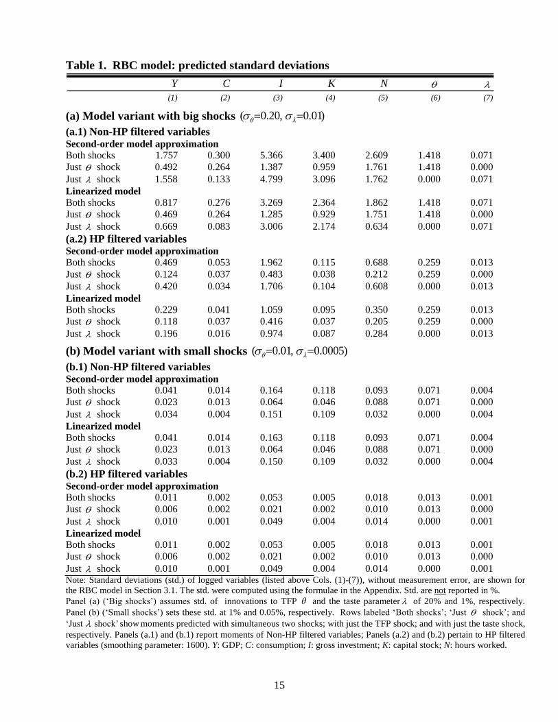
Predicted standard deviations Table 1 reports unconditional standard deviations of 7 logged variables (GDP, consumption,

investment, capital, hours, TFP and the taste shock ) generated by the first- and second-order

approximations.11

Model variants with both shocks, and variants with just one type of shock, are

considered; moments for non-HP (Hodrick-Prescott) filtered variables are shown, as well as

moments of HP filtered variables (smoothing parameter: 1600).

In the ‘big shocks’ model variant, the standard deviations of endogenous variables are

huge; e.g., with both shocks, the standard deviation of (non-HP filtered) GDP is 176% (82%)

under the second-order (first-order) approximation; GDP is thus about twice as volatile under the

second-order approximation (than in the linearized model).12

The capital stock, investment and

hours worked (non-HP filtered) are about one-half more volatile under the second-order

approximation than under the linear approximation. By contrast, consumption volatility is similar

across the two approximations. Consumption is much less volatile than GDP, due to the assumed

high risk aversion of the household. The preference shock ( ) is the main source of fluctuations

in the capital stock, GDP and investment; the TFP shock ( ) is the main driver of consumption.

The correlation between the second- and first-order approximations of a given variable is

noticeably below unity, in the model variant with big shocks: e.g., about 0.7 for capital and

investment, and 0.5 for GDP.

The ‘small shocks’ model variant generates much smaller standard deviations of

endogenous variables that are roughly in line with predicted moments reported in the RBC

literature (e.g., Kollmann (1996)); e.g., the predicted standard deviation of HP-filtered GDP and

investment are about 1% and 5%, respectively (with both shocks). With small shocks, it remains

true that variables are more volatile in the second-order model than in the linearized model,

however, the difference is barely noticeable. E.g., the ratio of the GDP [investment] standard

dev. across the 2nd

/1st order approximations is merely 1.005 [1.002].

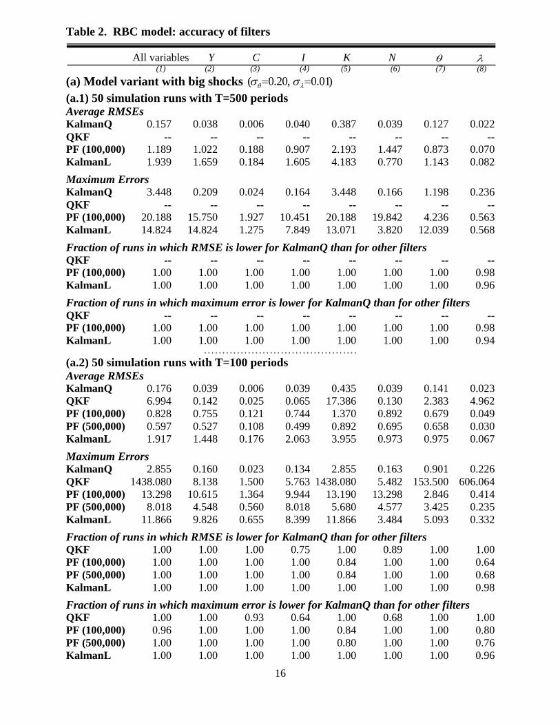
Filter accuracy

I generate 50 simulation runs of T=500 and of T=100 periods for the observables, using the

second-order (pruned) state equation of the RBC model. Each run is initialized at the

unconditional mean of the state vector. I apply the KalmanQ filter to the simulated observables

(with measurement error). I also use Ivashchenko’s (2013) Quadratic Kalman Filter ‘QKF’ and a

conventional Kalman filter, referred to as ‘KalmanL’ (that treats the linearized model (3) as the

true DGP). In addition, the standard particle filter (as described in An and Schorfheide (2007))--

11

The statistics in Table 1 are shown for variables without measurement error. The ranking of volatilities generated

by the two approximations and shocks is not affected by the presence of measurement error. 12

HP filtered variables are markedly less volatile than non-HP filtered variables; however, volatility remains much

higher under the second-order approximation than under the linear approximation, in the ‘big shocks’ variant. E.g.

the standard dev. of HP filtered GDP is 47% (23%) under the second- (first-) order approximation.

9

referred to a ‘PF(p)’, where p is the number of particles--is applied to the pruned state equation

(4); for the simulation runs with T=500 periods, 100,000 particles are employed; for runs with

T=100 periods, versions of the PF with 100,000 and with 500,000 particles are used.13

Accuracy

is evaluated for the 7 logged latent variables considered in Table 1.

In each simulation run s=1,..,50, the root mean square error (RMSE) is computed, across

all (logged) 7 variables,

2 1/ 21 71 1, , , ,7

( ( ) ) ,i iTi ts All s t s t tT

RMSE and separately for each individual

variable i=1,..7, 2 1/ 21

, 1 , , ,( ( ) ) ,T i i

s i t s t s t tRMSE

where ,

i

s t is the true date t value of variable i in

run s, while , ,

i

s t t is the filtered estimate (conditional expectation) of that variable, given the

date t information set. Table 2 reports RMSEs that are averaged across simulation runs. In the

Panels labeled ‘Average RMSEs’, Column (1) shows average RMSE, across all 7 variables, 501

1 ,50,s s ALLRMSE while Cols. (2)-(8) separately show average RMSEs for each individual

variable i, 5011 ,50

.s s iRMSE Also reported are maximum estimation errors across all variables,

periods and runs, as well as maximum estimation errors for each variable i (across all periods

and all simulation runs); see Panels labeled ‘Maximum Errors’. These accuracy measures are

reported for each of the filters (see rows labeled ‘KalmanQ’, ‘QKF’, ‘PF(100,000)’,

‘PF(500,000)’, and ‘KalmanL’). In addition, I report the fraction of simulation runs in which the

KalmanQ filter generates lower RMSEs and lower maximum estimation error than the other

filters.

Table 2 shows that the KalmanQ filter is more accurate than the PF and KalmanL filters,

in all (or almost all) simulation runs—this holds for both the ‘big shocks’ and ‘small shocks’

model variants.14

In all 50 simulation runs for the ‘big shocks’ model variant with T=500 periods

(see Panel (a.1)), the QKF generated time paths of filtered state estimates that diverged

explosively from the true states.15

That problem never arose for the KalmanQ filter. In the ‘big

shocks’ model variant with T=100 periods (see Panel (a.2)), the QKF exploded in 22 of the 50

simulation runs (44%); for that variant, the average RMSEs and maximum errors reported for the

QKF pertain to the simulation runs in which the QKF did not explode; in those simulation runs

the KalmanQ filter is markedly more accurate than the QKF. Average RMSEs generated by

KalmanQ are often orders of magnitudes smaller than the RMSEs generated by the particle filter,

and that even when 500,000 particles are used. E.g., for the simulation runs of the ‘big shocks’

model variant with T=100 periods, the average RMSEs for GDP are 0.039, 0.142, 0.755, 0.527

and 1.488, respectively, for KalmanQ, QKF, PF(100,000), PF(500,000), and KalmanL; the

corresponding maximum errors are 0.160, 8.138, 10.615, 4.548 and 9.826, respectively (see

Panel (a.2), Col. (2)).

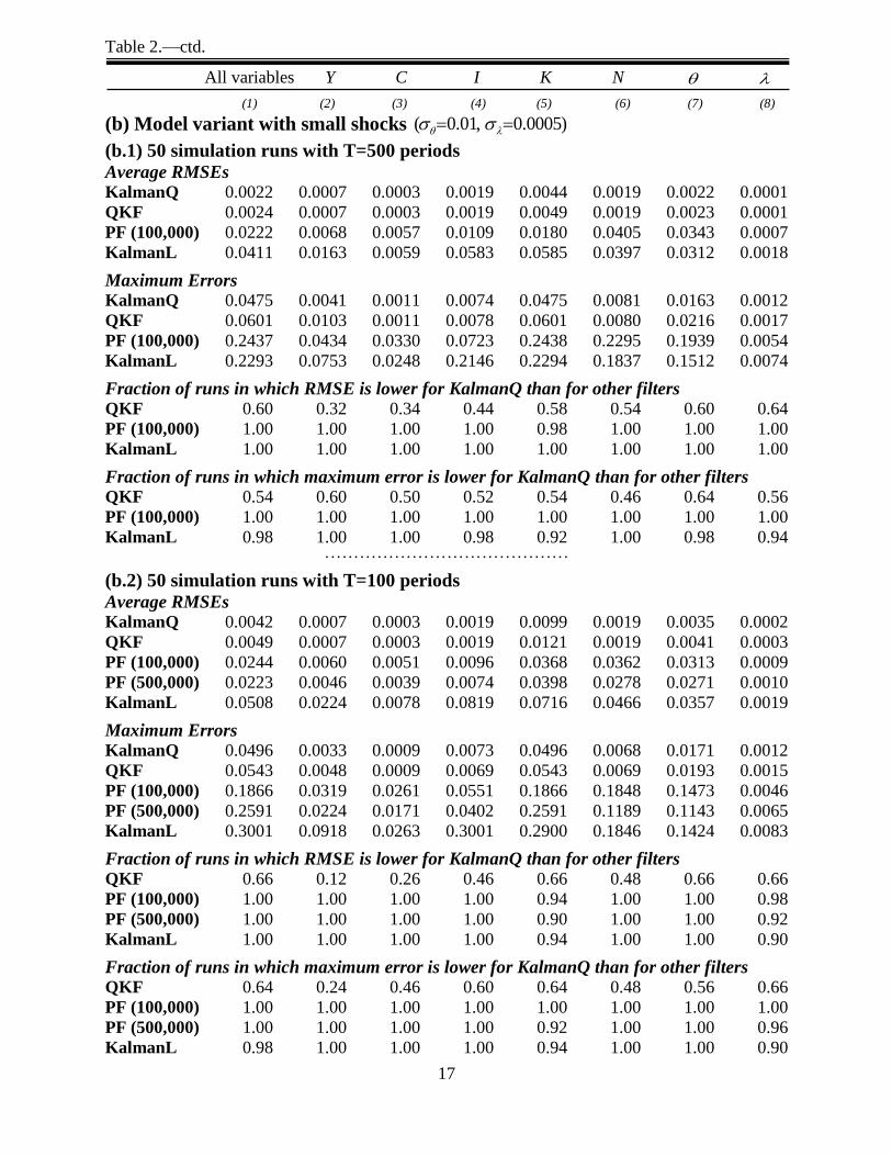
In the ‘small shocks’ simulation runs (Table 2, Panels (b.1) and (b.2)), all the filters are

more accurate than in the ‘big shocks’ simulations, and thus the absolute accuracy differences

between the filters are smaller. The QKF did not explode in the ‘small shocks’ simulations. The

13

I apply KalmanL to de-meaned series, as the linearized model implies that the unconditional mean of state

variables, expressed as differences from steady state, is zero, while variables generated from the second-order model

have a non-zero mean. The initial particles used for the particle filter are drawn from a multi-variate normal

distribution whose mean and variance are set to unconditional moments of the state vector. 14 I also computed median absolute errors (MAEs) for the filtered series. The results (available on request) confirm

the greater accuracy of the KalmanQ filter. 15

Once the QKF filtered estimates of the second-order accurate state variables ,t t reach large values, the one-step

ahead covariance matrix 1,t tV

takes huge values too (in the QKF, 1,t tV

depends on , );t t at that point the

observations are no longer able to correct the filtered series, and the filtered series may start to diverge explosively.

10

filtered estimates of latent states generated by the KalmanQ filter and by the QKF are now

broadly similar (across all variables, the KalmanQ filter is more accurate than the QKF in 54%-

66% of all simulation runs; see Column (1)). For the ‘small shocks’ simulation runs with T=100

periods, the average RMSEs for GDP are 0.0007, 0.0007, 0.0060, 0.0046 and 0.0224, for

KalmanQ, QKF, PF(100,000), PF(500,000) and KalmanL respectively, while corresponding

maximum errors are 0.0033, 0.0048, 0.0319, 0.0224 and 0.0918 (see Panel (b.2)). The relative

improvement in accuracy from using the KalmanQ filter thus remains sizable, relative to the

particle filter, and relative to KalmanL.

Note that the accuracy checks considered so far are based on pruned simulated sample

paths (generated using (3),(4)). It seems interesting to also apply the filters to sample paths

generated by the unpruned model (2). For the ’big shocks’ model variant, all unpruned sample

paths of length T=100 and T=500 explode. By contrast, for the ‘small shocks’ model variant, the

unpruned sample paths fail to explode—in fact, those paths are highly correlated with the pruned

sample paths; the performance of the filters is hence similar to that reported in Table 2, for the

‘small shocks’ pruned model variant.16

Detailed results are available on request.

Computing time

KalmanQ, QKF, the particle filters with 100,000 and 500,000 particles and KalmanL require

0.03, 0.05, 14.69, 81.21 and 0.01 seconds, respectively, to filter simulated series of T=100

periods generated by the RBC model, on a desktop computer with a 64-bit operating system and

a 3.4 Ghz processor. For series of T=500 periods, the corresponding computing times are 0.12,

0.21, 73.72, 401.58 and 0.04 seconds, respectively. Thus, the KalmanQ filter is about 500 (3000)

times faster than the particle filter with 100,000 (500,000) particles, and approximately 40%

faster than the QKF.

For a sufficiently large number of particles, the particle filter is (asymptotically) an exact

algorithm for computing the conditional expectation of the state vector. However, the

experiments in Table 2 suggest that a very large number of particles (above 500,000) is needed

to outperform KalmanQ; the computational cost of using such a large number of particles would

be substantial.

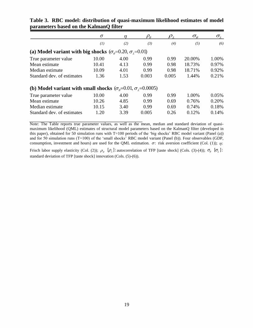
Evaluating the quasi-maximum likelihood (QML) parameter estimates

For 50 simulations runs of the ‘big shocks’ model variant and of the ‘small shocks’ variant, with

T=100 periods, I computed QML estimates of the risk aversion coefficient ( ), the labor supply

elasticity ( ), the autocorrelations of the forcing variables ( , ) and the standard deviations

of the innovations to the forcing variables ( , ). (As before, four observables are assumed:

GDP, consumption, investment and hours.) Table 3 reports the mean and median parameter

estimates, and the standard deviation of the parameter estimates, across the sample of 50

estimates per model variant. The parameters are tightly estimated; mean and median parameter

estimates are close to the true parameter values.17

3.2. State equations with randomly drawn coefficients Many other Monte Carlo experiments confirmed that the KalmanQ filter is competitive with the

particle filter, in terms of accuracy of the estimated state variables. To document the performance

16

For the unpruned ‘small shocks’ sample paths, the KalmanQ filter and the QKF thus have similar performance;

with T=100 [T=500], the KalmanQ filter is more accurate (across all variables) than the QKF in about 45% [54%] of

the simulation runs. 17

A more detailed evaluation of the small sample properties of the QML estimator is left for future research.

11

of the filter in a broad range of setting, I applied it to simulated data generated using variants of

the pruned state equations (3),(4) whose coefficients were drawn randomly from normal

distributions. Tables 4 reports moments of the resulting simulated latent state variables, while

Table 5 documents the accuracy of the filters. In both Tables, Panel (a) pertains to models with

n=20 variables, while Panel (b) assumes n=7 variables; I refer to the models in Panels (a) and (b)

as ‘medium models’, and as ‘small models’, respectively. In both set-ups, 7m independent

exogenous innovations are assumed, and the first four elements of the state vector t are

observed with measurement error ( 4).Yn The standard deviations of the (independent)

exogenous innovations 1( )t and of measurement errors ( )t are set at 1%.18

The elements of

0F are independent draws from N(0,1) that are scaled by a common factor so that the largest

element of 0F is 2(0.01) in absolute value. The elements of

1F are independent draws from

N(0,1) that are scaled by a common factor so that the largest eigenvalue of 1F has an absolute

value of 0.99. The elements of 2F are independent draws from N(0,1). In one set of simulations,

referred to as ‘strong curvature’ simulations, all elements of 11 12 22, ,F F F are independent draws

from N(0,1); in another set of simulations with ‘weak curvature’, the elements of 11 12 22, ,F F F are

independent draws from 2(0,(0.01) ),N so that curvature is much smaller, on average. For both

the ‘medium’ and ‘small’ model variants, 50 random ‘strong curvature’ coefficient sets, and 50

random ‘weak curvature’ coefficient sets were drawn. Thus, 200 different random sets of

coefficients 0 1 2 11 12 22( , , , , , )F F F F F F are considered. For each set of coefficients, the state equations

(3) and (4) were simulated over T=100 periods (each run was initialized at the unconditional

mean of the state vector), and the filters were applied to the observables (with measurement

error).

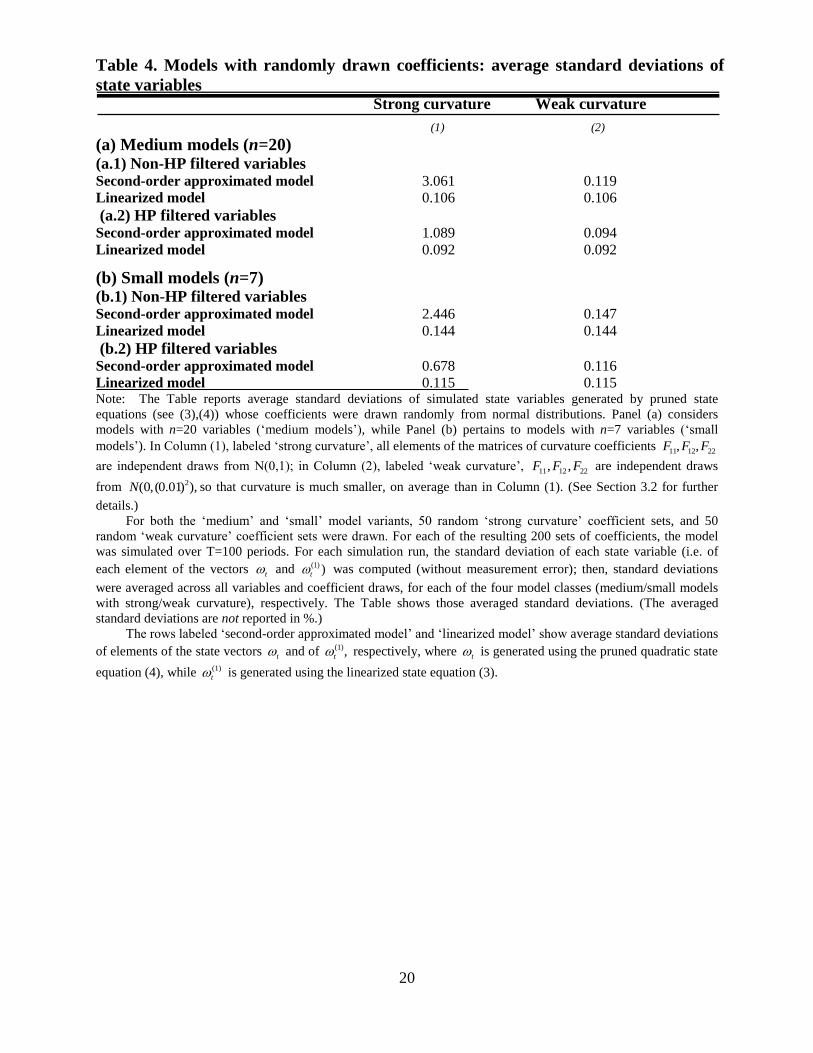
Table 4 reports (averaged) standard deviations of the latent state variables for the

‘medium’ and ‘small’ model variants with ‘strong curvature’ (Col. (1)) and with ‘weak

curvature’ (Col. (2)). The rows labeled ‘Second-order approximated model’ and ‘Linearized

model’ show (averaged) standard deviations of t and of (1),t respectively, where t was

generated using the pruned quadratic state equation (4), while (1)

t was generated using the linear

state equation (3).19

In ‘strong curvature’ model variants, the average predicted volatility of t

(second-order accurate) is several time larger than that of (1).t By contrast, in the ‘weak

curvature’ variants, the volatility of the second-order accurate variables is only slightly higher

than that of the first-order accurate variables.

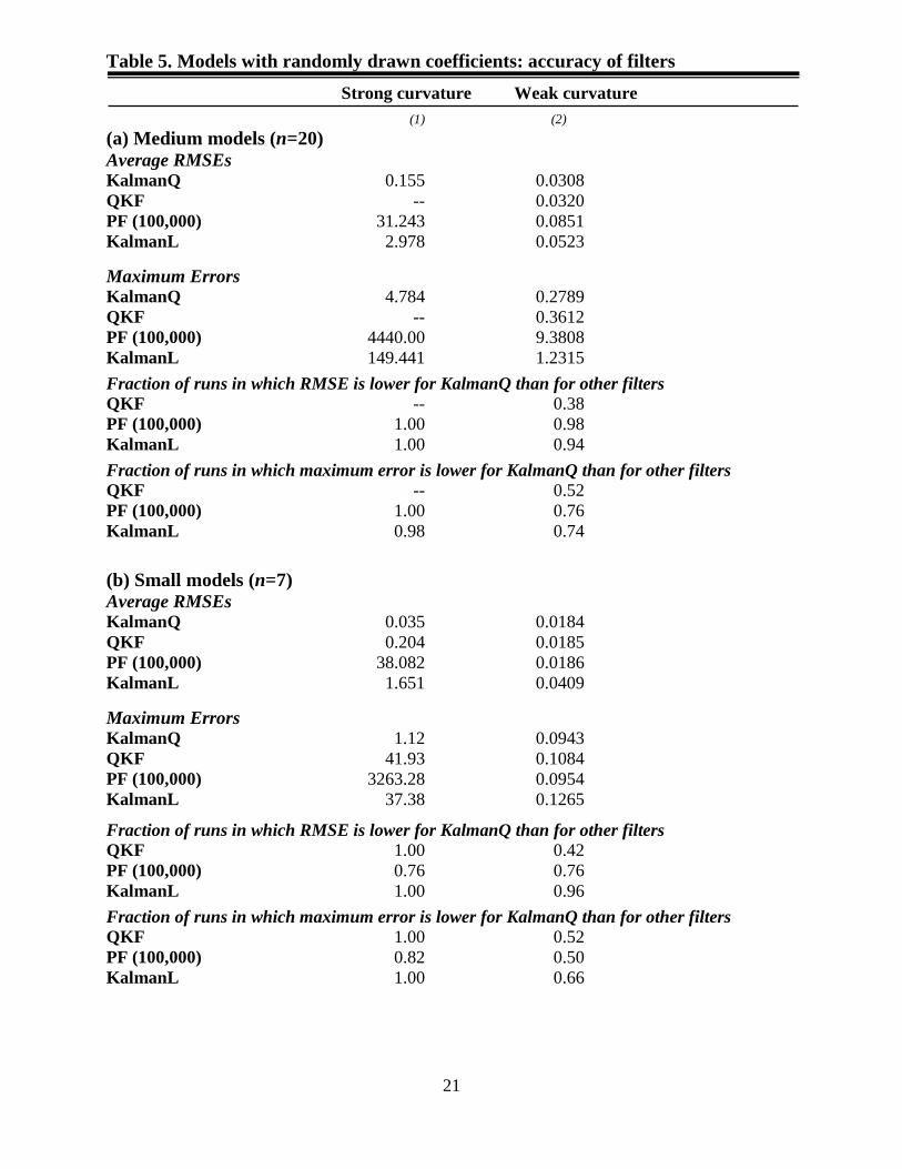
Table 5 compares the accuracy of the KalmanQ, QKF, PF(100,000) and KalmanL filters,

for each of the four model classes (medium/small models with strong/weak curvature). For each

model class, the KalmanQ filter generates lower average RMSEs and lower maximum errors

than the PF(100,000) and KalmanL filters. E.g., for the ‘medium models’, the average RMSEs of

18 2 2(.01) ; (.01) .

ym nI I As before, the parameter that scales the size of the shocks is normalized as 1.

19For each simulation run, the standard deviation of each element of t and (1)

t was computed; then, standard

deviations were averaged across variables and coefficient draws, for each of the four model classes (medium/small

models with strong/weak curvature).

12

KalmanQ, PF(100,000) and KalmanL are 0.155, 31.243 and 2.978, respectively, under ‘strong

curvature’, and 0.031, 0.085 and 0.052, respectively under ‘weak curvature’ (see Panel (a)).

The time paths of filtered estimates of state variables generated by the QKF exploded in

all simulation runs for ‘medium models’ with ‘strong curvature’. For ‘small models’ with ‘strong

curvature’, the QKF exploded in 48% of the simulation runs; for the runs where the QKF did not

explode, the KalmanQ filter is markedly more accurate than the QKF (see Column (1) of Panel

(b), Table 5). In the ‘weak curvature’ model variants, by contrast, the QKF did not explode in

any of the runs--KalmanQ is slightly more accurate than QKF in terms of average RMSEs and

Maximum Errors across all simulation runs.20

KalmanQ, QKF, PF(100,000) and KalmanL require 0.10, 0.14, 24.78 and 0.02 seconds,

respectively, to filter simulated series of T=100 periods generated by the ‘small models’; for

‘medium models’ the corresponding computing times are 0.86, 0.17, 78.49 and 0.03 seconds,

respectively. This confirms the finding that the KalmanQ filter is much faster than the particle

filter. The KalmanQ filter is faster than the QKF for ‘small models’, but not for ‘medium

models’.

4. Conclusion

This paper has developed a novel approach for the estimation of latent state variables in DSGE

models that are solved using a second-order accurate approximation and the ‘pruning’ scheme of

Kim, Kim, Schaumburg and Sims (2008). By contrast to particle filters, no stochastic simulations

are needed for the deterministic filter here; the present method is thus much faster than particle

filters. The use of the pruning scheme distinguishes the filter developed here from Ivashchenko’s

(2013) deterministic Quadratic Kalman filter (QKF). The present filter performs well even in

models with big shocks and high curvature. In Monte Carlo experiments, the filter developed

here generates more accurate estimates of latent state variables than the standard particle filter,

especially when the model has big shocks and high curvature. The present filter is also more

accurate than a Kalman filter that treats the linearized model as the true DGP. Due to its high

speed, the filter presented here is suited for the estimation of model parameters; a quasi-

maximum likelihood procedure can be used for that purpose.

20

I also examined filter performance using unpruned sample paths generated by the state equations with randomly

drawn coefficients (results available in request). All ‘strong curvature’ model variants generate exploding unpruned

sample paths. In the ‘weak curvature’ model variants, none of the unpruned sample path explodes--pruned and

unpruned sample paths are highly correlated; the QKF and KalmanQ filter show similar performance.

13

APPENDIX: Computing moments of the state vector (for KalmanQ filter formula)

The unconditional mean and variance of the state vector 1tZ of the augmented state equation

(5) are given by: 1

1 1 0( ) ( )tE Z I G G

and 1 1 1 1 1( ) ( ) ' ( )t t tV Z GV Z G V u , respectively. Stationarity

of 1tZ (which holds under the assumption that all eigenvalues of 1F are strictly inside the unit

circle) implies 1( ) ( ),t tE Z E Z 1( ) ( ).t tV Z V Z

Once 1( )tV u has been determined, 1( )tV Z can

efficiently be computed using a doubling algorithm. Note that (1)

1 20( )i

t t iiF F

and recall that

(1)

1 2 1 12 1 22 1 1[ ( ) ( ( ))].t t t t t tu G G G P E P

(A.1)

(1) (1)

1( ) 0, ( ) 0,t t tE E (1)

1 1(( ) ' ) 0,t t tE (1)

1 1(( ) ( ) ') 0t t tE P hold as 1t has mean zero

and is serially independent. Hence, the covariances between the first and second right-hand side

(rhs) terms in (A.1), and between the second and third rhs terms are zero. (0, )t N implies that

the unconditional mean of all third order products of elements of 1t is zero (Isserlis’ theorem):

1 1 0i j k

t t tE for all i,j,k=1,..,m, where 1

h

t is the h-th element of 1t . Thus the covariance

between the first and third rhs terms in (A.1) too is zero. Note that (1) (1)

1( ) ( ) ,t t tV V

with (1) (1)

1 1 2 2( ) ( ) ' '.t tV FV F F F Thus,

(1)

1 2 2 12 12 22 1 22( ) ' ( ( ) ) ' ( ( )) '.t t tV u G G G V G G V P G

(0, )t N implies that the covariance between 1 1

i j

t t and 1 1

r s

t t is

1 1 1 1 , , , ,( , )i j r s

t t t t i r j s i s j rCov for i,j,r,s=1,..,m,

where , 1 1( )i r

i r t tE . (See, e.g., Triantafyllopoulos (2002).) This formula allows to compute

1( ( )),tV P the covariance matrix of the vector

1 1 1 2 1 2 2 2 1 1 1

1 1 1 1 1 1 1 1 1 1 1 1 1 1 1 1 1( ) ( , ,..., , ,..., ,..., , , ).m m m m m m m m

t t t t t t t t t t t t t t t t tP

Conditional variance of state-form disturbance

To derive the formula for the conditional variance of 1tu ((10) in main text) these facts are used:

(i) (1) (1)

1 1 ,(( ) ' | ) ,t

t t t t tE with (1) (1)

, ( | ).t

t t tE

(ii) (1)(1) (1) (1) (1) (1) (1) (1) (1)

1 1 1 1 , , ,(( )( )'| ) (( ') ( ')| ) (( ')| ) ( ') .t t t

t t t t t t t t t t t t t t t tE E E V

(Note that (1) (1) (1) (1) (1)

, ( '| ) ( | ) ( | ) 't t t

t t t t t tV E E E (1) (1) (1) (1)

, ,( '| ) ' .t

t t t t t tE )

(iii) 1 1( ( ) ' | ) 0,t

t tE P

(1)

1 1( ( )( ) ' | ) 0t

t t tE P (due to Isserlis’ theorem). Thus, the

conditional covariance between the 1st and 3

rd rhs terms in (A.1) and between th 2

nd and 3

rd rhs

terms is zero.

14

References

An, S. and F. Schorfheide, 2007. Bayesian Analysis of DSGE models. Econometric Reviews 26, 113–172.

Andreasen, M., 2012. Non-Linear DSGE Models and the Central Difference Kalman Filter. Journal of

Applied Econometrics 28, 929-955.

Andreasen, M., Fernández-Villaverde, J. and J. Rubio-Ramírez, 2013. The Pruned State-Space System for

Non-Linear DSGE Models: Theory and Empirical Applications. NBER WP 18983.

Aruoba, S., L. Bocola and F. Schorfheide, 2012. A New Class of Nonlinear Time Series Models for the

Evaluation of DSGE Models. Working Paper, U MD and U Penn.

Collard, F., Juillard, M., 2001. Perturbation methods for rational expectations models. Working Paper,

GREMAQ and CEPREMAP.

Del Negro, M. and F. Schorfheide, 2011. Bayesian Macroeconometrics, in: The Oxford Handbook of

Bayesian Econometrics (J. Geweke, G. Koop and H. van Dijk, eds.), Oxford University Press, 293-389.

Fernández-Villaverde, J. and J. Rubio-Ramírez, 2007. Estimating Macroeconomic Models: a Likelihood

Approach. Review of Economic Studies 74, 1059–1087.

Hamilton, J., 1994. Time Series Analysis. Princeton University Press.

Harvey, A., 1989. Forecasting—Structural Time Series Models and the Kalman Filter. Cambridge

University Press.

Ivashchenko, S. 2013. DSGE Model Estimation on the Basis of Second-Order Approximation.

Forthcoming, Computational Economics.

Jin, H., Judd, K., 2004. Applying PertSolv to Complete Market RBC models. Working paper, Stanford.

University.

Julier, S. and J. Uhlmann, 2004. Unscented Filtering and Nonlinear Estimation, Proceedings of the IEEE

92, 401-422.

Kim, J., Kim, S., Schaumburg, E. and C. Sims, 2008. Calculating and Using Second-Order Accurate

Solutions of Discrete-Time Dynamic Equilibrium Models, Journal of Economic Dynamics and Control

32, 3397-3414.

Kollmann, R., 1996. Incomplete Asset Markets and the Cross-Country Consumption Correlation Puzzle,

Journal of Economic Dynamics and Control 20, 945-962.

Kollmann, R., 2002. Monetary Policy Rules in the Open Economy: Effects of Welfare and Business

Cycles, Journal of Monetary Economics 49, 989-1015.

Kollmann, R., 2004. Solving Non-Linear Rational Expectations Models: Approximations based on Taylor

Expansions, Working Paper, University of Paris XII.

Kollmann, R., H.S. Kim and J. Kim, 2011. Solving the Multi-Country Real Business Cycle Model Using

a Perturbation Method, Journal of Economic Dynamics and Control 35, 203-206.

Lombardo, G. and A. Sutherland, 2007. Computing Second-Order Accurate Solutions for Rational

Expectation Models Using Linear Solution Methods. Journal of Economic Dynamics and Control 31,

515-530.

Norgaard, M., N. Poulsen and O. Ravn, 2000. New Developments in State Estimation for Nonlinear

Systems, Automatica 36, 1627-1638.

Schmitt-Grohé, S. and M. Uribe, 2004. Solving Dynamic General Equilibrium Models Using a Second-

Order Approximation to the Policy Function. Journal of Economic Dynamics and Control 28, 755 –

775.

Sims, C., 2000. Second Order Accurate Solution of Discrete Time Dynamic Equilibrium Models.

Working Paper, Economics Department, Princeton University

Smets, F. and R. Wouters, 2007. Shocks and Frictions in US Business Cycles: A Bayesian DSGE

Approach. American Economic Review 97, 586-660.

Lombardo, G. and A. Sutherland, 2007. Computing Second-Order-Accurate Solutions for Rational

Expectation Models Using Linear Solution Methods, Journal of Economic Dynamics and Control 31,

515-530.

Triantafyllopoulos, K., 2002. Moments and Cumulants of the Multivariate Real and Complex Gaussian

Distributions. Working Paper, University of Bristol.

15

Table 1. RBC model: predicted standard deviations

Y C I K N

(1) (2) (3) (4) (5) (6) (7)

(a) Model variant with big shocks ( 0.20, 0.01)

(a.1) Non-HP filtered variables Second-order model approximation

Both shocks 1.757 0.300 5.366 3.400 2.609 1.418 0.071

Just shock 0.492 0.264 1.387 0.959 1.761 1.418 0.000

Just shock 1.558 0.133 4.799 3.096 1.762 0.000 0.071

Linearized model

Both shocks 0.817 0.276 3.269 2.364 1.862 1.418 0.071

Just shock 0.469 0.264 1.285 0.929 1.751 1.418 0.000

Just shock 0.669 0.083 3.006 2.174 0.634 0.000 0.071

(a.2) HP filtered variables Second-order model approximation

Both shocks 0.469 0.053 1.962 0.115 0.688 0.259 0.013

Just shock 0.124 0.037 0.483 0.038 0.212 0.259 0.000

Just shock 0.420 0.034 1.706 0.104 0.608 0.000 0.013

Linearized model

Both shocks 0.229 0.041 1.059 0.095 0.350 0.259 0.013

Just shock 0.118 0.037 0.416 0.037 0.205 0.259 0.000

Just shock 0.196 0.016 0.974 0.087 0.284 0.000 0.013

(b) Model variant with small shocks ( 0.01, 0.0005)

(b.1) Non-HP filtered variables Second-order model approximation

Both shocks 0.041 0.014 0.164 0.118 0.093 0.071 0.004

Just shock 0.023 0.013 0.064 0.046 0.088 0.071 0.000

Just shock 0.034 0.004 0.151 0.109 0.032 0.000 0.004

Linearized model

Both shocks 0.041 0.014 0.163 0.118 0.093 0.071 0.004

Just shock 0.023 0.013 0.064 0.046 0.088 0.071 0.000

Just shock 0.033 0.004 0.150 0.109 0.032 0.000 0.004

(b.2) HP filtered variables Second-order model approximation

Both shocks 0.011 0.002 0.053 0.005 0.018 0.013 0.001

Just shock 0.006 0.002 0.021 0.002 0.010 0.013 0.000

Just shock 0.010 0.001 0.049 0.004 0.014 0.000 0.001

Linearized model

Both shocks 0.011 0.002 0.053 0.005 0.018 0.013 0.001

Just shock 0.006 0.002 0.021 0.002 0.010 0.013 0.000

Just shock 0.010 0.001 0.049 0.004 0.014 0.000 0.001 Note: Standard deviations (std.) of logged variables (listed above Cols. (1)-(7)), without measurement error, are shown for

the RBC model in Section 3.1. The std. were computed using the formulae in the Appendix. Std. are not reported in %.

Panel (a) (‘Big shocks’) assumes std. of innovations to TFP and the taste parameter of 20% and 1%, respectively.

Panel (b) (‘Small shocks’) sets these std. at 1% and 0.05%, respectively. Rows labeled ‘Both shocks’; ‘Just shock’; and

‘Just shock’ show moments predicted with simultaneous two shocks; with just the TFP shock; and with just the taste shock,

respectively. Panels (a.1) and (b.1) report moments of Non-HP filtered variables; Panels (a.2) and (b.2) pertain to HP filtered

variables (smoothing parameter: 1600). Y: GDP; C: consumption; I: gross investment; K: capital stock; N: hours worked.

16

Table 2. RBC model: accuracy of filters

All variables Y C I K N (1) (2) (3) (4) (5) (6) (7) (8)


(a.1) 50 simulation runs with T=500 periods Average RMSEs KalmanQ 0.157 0.038 0.006 0.040 0.387 0.039 0.127 0.022

QKF -- -- -- -- -- -- -- --

PF (100,000) 1.189 1.022 0.188 0.907 2.193 1.447 0.873 0.070

KalmanL 1.939 1.659 0.184 1.605 4.183 0.770 1.143 0.082

Maximum Errors KalmanQ 3.448 0.209 0.024 0.164 3.448 0.166 1.198 0.236

QKF -- -- -- -- -- -- -- --

PF (100,000) 20.188 15.750 1.927 10.451 20.188 19.842 4.236 0.563

KalmanL 14.824 14.824 1.275 7.849 13.071 3.820 12.039 0.568

Fraction of runs in which RMSE is lower for KalmanQ than for other filters QKF -- -- -- -- -- -- -- --

PF (100,000) 1.00 1.00 1.00 1.00 1.00 1.00 1.00 0.98

KalmanL 1.00 1.00 1.00 1.00 1.00 1.00 1.00 0.96

Fraction of runs in which maximum error is lower for KalmanQ than for other filters QKF -- -- -- -- -- -- -- --

PF (100,000) 1.00 1.00 1.00 1.00 1.00 1.00 1.00 0.98

KalmanL 1.00 1.00 1.00 1.00 1.00 1.00 1.00 0.94 . . . . . . . . . . . . . . . . . . . . . . . . . . . . . . . . . . . . . . . . . .

(a.2) 50 simulation runs with T=100 periods

Average RMSEs KalmanQ 0.176 0.039 0.006 0.039 0.435 0.039 0.141 0.023

QKF 6.994 0.142 0.025 0.065 17.386 0.130 2.383 4.962

PF (100,000) 0.828 0.755 0.121 0.744 1.370 0.892 0.679 0.049

PF (500,000) 0.597 0.527 0.108 0.499 0.892 0.695 0.658 0.030

KalmanL 1.917 1.448 0.176 2.063 3.955 0.973 0.975 0.067


QKF 1438.080 8.138 1.500 5.763 1438.080 5.482 153.500 606.064

PF (100,000) 13.298 10.615 1.364 9.944 13.190 13.298 2.846 0.414

PF (500,000) 8.018 4.548 0.560 8.018 5.680 4.577 3.425 0.235

KalmanL 11.866 9.826 0.655 8.399 11.866 3.484 5.093 0.332

Fraction of runs in which RMSE is lower for KalmanQ than for other filters QKF 1.00 1.00 1.00 0.75 1.00 0.89 1.00 1.00

PF (100,000) 1.00 1.00 1.00 1.00 0.84 1.00 1.00 0.64

PF (500,000) 1.00 1.00 1.00 1.00 0.84 1.00 1.00 0.68

KalmanL 1.00 1.00 1.00 1.00 1.00 1.00 1.00 0.98

Fraction of runs in which maximum error is lower for KalmanQ than for other filters QKF 1.00 1.00 0.93 0.64 1.00 0.68 1.00 1.00

PF (100,000) 0.96 1.00 1.00 1.00 0.84 1.00 1.00 0.80

PF (500,000) 1.00 1.00 1.00 1.00 0.80 1.00 1.00 0.76

KalmanL 1.00 1.00 1.00 1.00 1.00 1.00 1.00 0.96

17

Table 2.—ctd.

All variables Y C I K N

(1) (2) (3) (4) (5) (6) (7) (8)


(b.1) 50 simulation runs with T=500 periods


QKF 0.0024 0.0007 0.0003 0.0019 0.0049 0.0019 0.0023 0.0001

PF (100,000) 0.0222 0.0068 0.0057 0.0109 0.0180 0.0405 0.0343 0.0007

KalmanL 0.0411 0.0163 0.0059 0.0583 0.0585 0.0397 0.0312 0.0018


QKF 0.0601 0.0103 0.0011 0.0078 0.0601 0.0080 0.0216 0.0017

PF (100,000) 0.2437 0.0434 0.0330 0.0723 0.2438 0.2295 0.1939 0.0054

KalmanL 0.2293 0.0753 0.0248 0.2146 0.2294 0.1837 0.1512 0.0074


PF (100,000) 1.00 1.00 1.00 1.00 0.98 1.00 1.00 1.00

KalmanL 1.00 1.00 1.00 1.00 1.00 1.00 1.00 1.00


PF (100,000) 1.00 1.00 1.00 1.00 1.00 1.00 1.00 1.00

KalmanL 0.98 1.00 1.00 0.98 0.92 1.00 0.98 0.94 . . . . . . . . . . . . . . . . . . . . . . . . . . . . . . . . . . . . . . . . . .

(b.2) 50 simulation runs with T=100 periods


QKF 0.0049 0.0007 0.0003 0.0019 0.0121 0.0019 0.0041 0.0003

PF (100,000) 0.0244 0.0060 0.0051 0.0096 0.0368 0.0362 0.0313 0.0009

PF (500,000) 0.0223 0.0046 0.0039 0.0074 0.0398 0.0278 0.0271 0.0010

KalmanL 0.0508 0.0224 0.0078 0.0819 0.0716 0.0466 0.0357 0.0019


QKF 0.0543 0.0048 0.0009 0.0069 0.0543 0.0069 0.0193 0.0015

PF (100,000) 0.1866 0.0319 0.0261 0.0551 0.1866 0.1848 0.1473 0.0046

PF (500,000) 0.2591 0.0224 0.0171 0.0402 0.2591 0.1189 0.1143 0.0065

KalmanL 0.3001 0.0918 0.0263 0.3001 0.2900 0.1846 0.1424 0.0083


PF (100,000) 1.00 1.00 1.00 1.00 0.94 1.00 1.00 0.98

PF (500,000) 1.00 1.00 1.00 1.00 0.90 1.00 1.00 0.92

KalmanL 1.00 1.00 1.00 1.00 0.94 1.00 1.00 0.90


PF (100,000) 1.00 1.00 1.00 1.00 1.00 1.00 1.00 1.00

PF (500,000) 1.00 1.00 1.00 1.00 0.92 1.00 1.00 0.96

KalmanL 0.98 1.00 1.00 1.00 0.94 1.00 1.00 0.90

18

Table 2.—ctd.

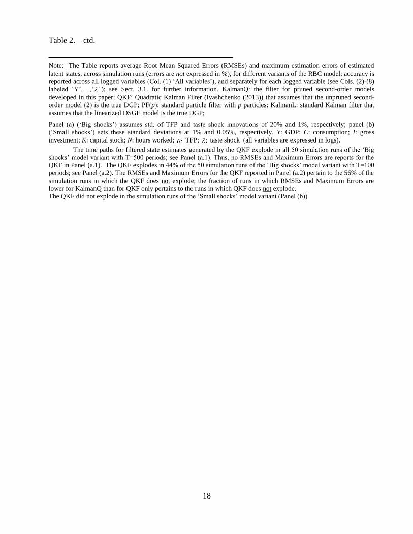
Note: The Table reports average Root Mean Squared Errors (RMSEs) and maximum estimation errors of estimated

latent states, across simulation runs (errors are not expressed in %), for different variants of the RBC model; accuracy is

reported across all logged variables (Col. (1) ‘All variables’), and separately for each logged variable (see Cols. (2)-(8)

labeled ‘Y’,…, ' ' ); see Sect. 3.1. for further information. KalmanQ: the filter for pruned second-order models

developed in this paper; QKF: Quadratic Kalman Filter (Ivashchenko (2013)) that assumes that the unpruned second-

order model (2) is the true DGP; PF(p): standard particle filter with p particles: KalmanL: standard Kalman filter that

assumes that the linearized DSGE model is the true DGP;

Panel (a) (‘Big shocks’) assumes std. of TFP and taste shock innovations of 20% and 1%, respectively; panel (b)

(‘Small shocks’) sets these standard deviations at 1% and 0.05%, respectively. Y: GDP; C: consumption; I: gross

investment; K: capital stock; N: hours worked; : TFP; : taste shock (all variables are expressed in logs).

The time paths for filtered state estimates generated by the QKF explode in all 50 simulation runs of the ‘Big

shocks’ model variant with T=500 periods; see Panel (a.1). Thus, no RMSEs and Maximum Errors are reports for the

QKF in Panel (a.1). The QKF explodes in 44% of the 50 simulation runs of the ‘Big shocks’ model variant with T=100

periods; see Panel (a.2). The RMSEs and Maximum Errors for the QKF reported in Panel (a.2) pertain to the 56% of the

simulation runs in which the QKF does not explode; the fraction of runs in which RMSEs and Maximum Errors are

lower for KalmanQ than for QKF only pertains to the runs in which QKF does not explode.

The QKF did not explode in the simulation runs of the ‘Small shocks’ model variant (Panel (b)).

19

Table 3. RBC model: distribution of quasi-maximum likelihood estimates of model

parameters based on the KalmanQ filter

(1) (2) (3) (4) (5) (6)


True parameter value 10.00 4.00 0.99 0.99 20.00% 1.00%

Mean estimate 10.41 4.13 0.99 0.98 18.73% 0.97%

Median estimate 10.09 4.01 0.99 0.98 18.71% 0.92%

Standard dev. of estimates 1.36 1.53 0.003 0.005 1.44% 0.21%


True parameter value 10.00 4.00 0.99 0.99 1.00% 0.05%

Mean estimate 10.26 4.85 0.99 0.69 0.76% 0.20%

Median estimate 10.15 3.40 0.99 0.69 0.74% 0.18%

Standard dev. of estimates 1.20 3.39 0.005 0.26 0.12% 0.14%

Note: The Table reports true parameter values, as well as the mean, median and standard deviation of quasi-

maximum likelihood (QML) estimates of structural model parameters based on the KalmanQ filter (developed in

this paper), obtained for 50 simulation runs with T=100 periods of the ‘big shocks’ RBC model variant (Panel (a))

and for 50 simulation runs (T=100) of the ‘small shocks’ RBC model variant (Panel (b)). Four observables (GDP,

consumption, investment and hours) are used for the QML estimation. : risk aversion coefficient (Col. (1)); :

Frisch labor supply elasticity (Col. (2)); [ ] : autocorrelation of TFP [taste shock] (Cols. (3)-(4)); [ ] :

standard deviation of TFP [taste shock] innovation (Cols. (5)-(6)).

20

Table 4. Models with randomly drawn coefficients: average standard deviations of

state variables Strong curvature Weak curvature

(1) (2)

(a) Medium models (n=20) (a.1) Non-HP filtered variables Second-order approximated model 3.061 0.119

Linearized model 0.106 0.106

(a.2) HP filtered variables Second-order approximated model 1.089 0.094


(b) Small models (n=7) (b.1) Non-HP filtered variables Second-order approximated model 2.446 0.147


(b.2) HP filtered variables Second-order approximated model 0.678 0.116

Linearized model 0.115 0.115 Note: The Table reports average standard deviations of simulated state variables generated by pruned state

equations (see (3),(4)) whose coefficients were drawn randomly from normal distributions. Panel (a) considers

models with n=20 variables (‘medium models’), while Panel (b) pertains to models with n=7 variables (‘small

models’). In Column (1), labeled ‘strong curvature’, all elements of the matrices of curvature coefficients 11 12 22, ,F F F

are independent draws from N(0,1); in Column (2), labeled ‘weak curvature’, 11 12 22, ,F F F are independent draws

from 2(0,(0.01) ),N so that curvature is much smaller, on average than in Column (1). (See Section 3.2 for further

details.)

For both the ‘medium’ and ‘small’ model variants, 50 random ‘strong curvature’ coefficient sets, and 50

random ‘weak curvature’ coefficient sets were drawn. For each of the resulting 200 sets of coefficients, the model

was simulated over T=100 periods. For each simulation run, the standard deviation of each state variable (i.e. of

each element of the vectors t and

(1) )t was computed (without measurement error); then, standard deviations

were averaged across all variables and coefficient draws, for each of the four model classes (medium/small models

with strong/weak curvature), respectively. The Table shows those averaged standard deviations. (The averaged

standard deviations are not reported in %.)

The rows labeled ‘second-order approximated model’ and ‘linearized model’ show average standard deviations

of elements of the state vectors t and of (1),t respectively, where t is generated using the pruned quadratic state

equation (4), while (1)

t is generated using the linearized state equation (3).

21

Table 5. Models with randomly drawn coefficients: accuracy of filters

Strong curvature Weak curvature

(1) (2)

(a) Medium models (n=20)

Average RMSEs KalmanQ 0.155 0.0308

QKF -- 0.0320

PF (100,000) 31.243 0.0851

KalmanL 2.978 0.0523

Maximum Errors KalmanQ 4.784 0.2789

QKF -- 0.3612

PF (100,000) 4440.00 9.3808

KalmanL 149.441 1.2315

Fraction of runs in which RMSE is lower for KalmanQ than for other filters

QKF -- 0.38

PF (100,000) 1.00 0.98

KalmanL 1.00 0.94

Fraction of runs in which maximum error is lower for KalmanQ than for other filters

QKF -- 0.52

PF (100,000) 1.00 0.76

KalmanL 0.98 0.74

(b) Small models (n=7) Average RMSEs KalmanQ 0.035 0.0184

QKF 0.204 0.0185

PF (100,000) 38.082 0.0186

KalmanL 1.651 0.0409

Maximum Errors KalmanQ 1.12 0.0943

QKF 41.93 0.1084

PF (100,000) 3263.28 0.0954

KalmanL 37.38 0.1265

Fraction of runs in which RMSE is lower for KalmanQ than for other filters

QKF 1.00 0.42

PF (100,000) 0.76 0.76

KalmanL 1.00 0.96

Fraction of runs in which maximum error is lower for KalmanQ than for other filters

QKF 1.00 0.52

PF (100,000) 0.82 0.50

KalmanL 1.00 0.66

22

Table 5.—ctd.

Note: The Table reports average Root Mean Squared Errors (RMSEs) and maximum estimation errors of estimated

latent variables produced by four filters, across simulation runs and state variables, for versions of the pruned state

equation (4) with randomly drawn coefficients; see Section 3.2. Panel (a) (‘medium models’) assumes n=20 variables;

Panel (b) (‘small model’) assumes n=7 variables. In ‘strong curvature’ [‘weak curvature’] experiments (see Column 1

[2]), all elements of the matrices of curvature coefficients 11 12 22, ,F F F are independent draws from N(0,1) [N(0,(0.01)2].

(See Section 3.2 for further details.) For both the ‘medium’ and ‘small’ model variants, 50 random ‘strong curvature’

coefficient sets, and 50 random ‘weak curvature’ coefficient sets were drawn. For each of the resulting 200 sets of

coefficient, the model was simulated over T=100 periods.

For each simulation run, the RMSE and the maximal error was computed, for each of the ‘n’ estimated latent

variables; then, RMSEs were averaged across variables and coefficient draws, for each of the four model classes

(medium/small models with strong/weak curvature); maximum errors were likewise determined across all n variables,

and across all draws, for each of the four model classes.

KalmanQ: the filter for pruned second-order models developed in this paper; QKF: Quadratic Kalman Filter

(Ivashchenko (2013)) that assumes that the unpruned second-order model (2) is the true DGP; PF(p): standard particle

filter with p particles: KalmanL: standard Kalman filter that assumes that the linearized model is the true DGP.

The time paths for filtered estimates of the state variables generated by the QKF explode in all 50 simulation runs

of the ‘medium models’ with ‘strong curvature’; thus, no RMSEs and Maximum Errors are reported for the Quadratic

Kalman Filter (QKF) in Column (1) of Panel (a).

The QKF explodes in 48% of the 50 simulation runs of the ‘small models’ with ‘strong curvature’; the RMSEs

and Maximum Errors for the QKF reported in Column (1) of Panel (b) pertain to the 52% of the simulation runs in

which the QKF does not explode; the reported fraction of runs in which RMSEs and Maximum Errors are lower for

KalmanQ than for QKF likewise only pertains to the runs in which QKF does not explode.

The QKF did not explode in the simulation runs of the ‘weak curvature’ model variants (Column (2)).

forthcoming in: computational economics€¦ · forthcoming in: computational economics tractable...

Documents