fors data reduction cookbook - eso...0.1 12/08/07 all draft version 1.1 27/08/07 first version fors...
TRANSCRIPT

EUROPEAN SOUTHERN OBSERVATORY
Organisation Europeene pour des Recherches Astronomiques dans l’Hemisphere AustralEuropaische Organisation fur astronomische Forschung in der sudlichen Hemisphare
ESO - European Southern ObservatoryKarl-Schwarzschild Str. 2, D-85748 Garching bei Munchen
Very Large Telescope
Paranal Science Operations
FORS data reduction cookbook
Doc. No. VLT-MAN-ESO-13100-4030
Issue 1.1, Date 27/08/2007
K. O’BrienPrepared . . . . . . . . . . . . . . . . . . . . . . . . . . . . . . . . . . . . . . . . . .
Date Signature
G. MarconiApproved . . . . . . . . . . . . . . . . . . . . . . . . . . . . . . . . . . . . . . . . . .
Date Signature
O. HainautReleased . . . . . . . . . . . . . . . . . . . . . . . . . . . . . . . . . . . . . . . . . .
Date Signature

FORS data reduction cookbook VLT-MAN-ESO-13100-4030 ii
This page was intentionally left blank

FORS data reduction cookbook VLT-MAN-ESO-13100-4030 iii
Change Record
Issue/Rev. Date Section/Parag. affected Reason/Initiation/Documents/Remarks
0.1 12/08/07 All Draft version1.1 27/08/07 First version

FORS data reduction cookbook VLT-MAN-ESO-13100-4030 iv
This page was intentionally left blank

FORS data reduction cookbook VLT-MAN-ESO-13100-4030 v
Contents
1 Introduction 1
1.1 Purpose . . . . . . . . . . . . . . . . . . . . . . . . . . . . . . . . . . . . . . . 1
1.2 Reference documents and papers . . . . . . . . . . . . . . . . . . . . . . . . . 1
1.3 Abbreviations and acronyms . . . . . . . . . . . . . . . . . . . . . . . . . . . . 1
1.4 Stylistic conventions . . . . . . . . . . . . . . . . . . . . . . . . . . . . . . . . 1
2 Imaging 3
2.1 Introduction . . . . . . . . . . . . . . . . . . . . . . . . . . . . . . . . . . . . . 3
2.2 Flat field . . . . . . . . . . . . . . . . . . . . . . . . . . . . . . . . . . . . . . . 3
2.2.1 Simple methods . . . . . . . . . . . . . . . . . . . . . . . . . . . . . . . 5
2.2.2 Advanced Methods . . . . . . . . . . . . . . . . . . . . . . . . . . . . . 6
2.2.3 Estimate the quality of the flatfied . . . . . . . . . . . . . . . . . . . . 10
2.3 Sky subtraction and normalization . . . . . . . . . . . . . . . . . . . . . . . . 11
2.4 Combination of frames . . . . . . . . . . . . . . . . . . . . . . . . . . . . . . . 11
2.4.1 Centering . . . . . . . . . . . . . . . . . . . . . . . . . . . . . . . . . . 11
2.4.2 Co-adding . . . . . . . . . . . . . . . . . . . . . . . . . . . . . . . . . . 12
3 FORS long-slit data reduction 14
3.1 Introduction . . . . . . . . . . . . . . . . . . . . . . . . . . . . . . . . . . . . . 14
3.2 Processing the calibration data . . . . . . . . . . . . . . . . . . . . . . . . . . 14
3.2.1 Running the recipe fors calib . . . . . . . . . . . . . . . . . . . . . . . 15
3.2.2 Checking the results . . . . . . . . . . . . . . . . . . . . . . . . . . . . 16
3.2.3 Troubleshooting . . . . . . . . . . . . . . . . . . . . . . . . . . . . . . . 17
3.3 Processing the scientific data . . . . . . . . . . . . . . . . . . . . . . . . . . . . 18
3.3.1 Running the recipe fors science . . . . . . . . . . . . . . . . . . . . . . 19
3.3.2 Checking the results . . . . . . . . . . . . . . . . . . . . . . . . . . . . 20
3.3.3 Troubleshooting . . . . . . . . . . . . . . . . . . . . . . . . . . . . . . . 21
4 FORS MOS/MXU data reduction 23
4.1 Introduction . . . . . . . . . . . . . . . . . . . . . . . . . . . . . . . . . . . . . 23
4.2 Processing the calibration data . . . . . . . . . . . . . . . . . . . . . . . . . . 23
4.2.1 Running the recipe fors calib . . . . . . . . . . . . . . . . . . . . . . . 24
4.2.2 Checking the results . . . . . . . . . . . . . . . . . . . . . . . . . . . . 26
4.2.3 Troubleshooting . . . . . . . . . . . . . . . . . . . . . . . . . . . . . . . 29
4.3 Processing the scientific data . . . . . . . . . . . . . . . . . . . . . . . . . . . . 34
4.3.1 Running the recipe fors science . . . . . . . . . . . . . . . . . . . . . . 34
4.3.2 Checking the results . . . . . . . . . . . . . . . . . . . . . . . . . . . . 36
4.3.3 Troubleshooting . . . . . . . . . . . . . . . . . . . . . . . . . . . . . . . 38
5 Multi Object Spectroscopy 41

FORS data reduction cookbook VLT-MAN-ESO-13100-4030 vi
5.1 Introduction . . . . . . . . . . . . . . . . . . . . . . . . . . . . . . . . . . . . . 41
5.2 Basic reduction steps . . . . . . . . . . . . . . . . . . . . . . . . . . . . . . . . 41
5.2.1 Removing the detector bias . . . . . . . . . . . . . . . . . . . . . . . . 41
5.2.2 Flat fielding . . . . . . . . . . . . . . . . . . . . . . . . . . . . . . . . . 43
5.2.3 Mapping the slit curvature . . . . . . . . . . . . . . . . . . . . . . . . . 48
5.2.4 Applying the distortion correction (optional and not recommended) . . 51
5.2.5 Image combining and sky subtraction . . . . . . . . . . . . . . . . . . 52
5.2.6 Object extraction . . . . . . . . . . . . . . . . . . . . . . . . . . . . . . 54
5.3 Wavelength Calibration . . . . . . . . . . . . . . . . . . . . . . . . . . . . . . . 55
5.4 Flux Calibration . . . . . . . . . . . . . . . . . . . . . . . . . . . . . . . . . . 57
6 HIgh Time resolution (HIT) modes 60
6.1 Introduction . . . . . . . . . . . . . . . . . . . . . . . . . . . . . . . . . . . . . 60
6.2 general comments . . . . . . . . . . . . . . . . . . . . . . . . . . . . . . . . . . 61
6.3 High time resolution imaging (HIT-I) . . . . . . . . . . . . . . . . . . . . . . . 61
6.4 High time resolution spectroscopy (HIT-MS) . . . . . . . . . . . . . . . . . . . 61
6.4.1 Preparation . . . . . . . . . . . . . . . . . . . . . . . . . . . . . . . . . 61
6.4.2 Tracing the spectra . . . . . . . . . . . . . . . . . . . . . . . . . . . . . 63
6.4.3 Extracting the target and sky spectra . . . . . . . . . . . . . . . . . . . 65
6.4.4 fixing the header items . . . . . . . . . . . . . . . . . . . . . . . . . . . 69
6.4.5 extracting the arcs . . . . . . . . . . . . . . . . . . . . . . . . . . . . . 70
6.4.6 extracting the flux standard . . . . . . . . . . . . . . . . . . . . . . . . 70
A Reducing FORS data using the pipeline recipes 71
A.1 Overview . . . . . . . . . . . . . . . . . . . . . . . . . . . . . . . . . . . . . . . 71
A.2 Launching pipeline recipes: Gasgano and Esorex . . . . . . . . . . . . . . . . . 71

FORS data reduction cookbook VLT-MAN-ESO-13100-4030 1
1 Introduction
FORS is the visual and near-UV FOcal Reducer and low dispersion Spectrograph for theVery Large Telescope (VLT). Two versions of FORS have been built and are installed on thecassegrain foci of two of the unit telescopes that comprise the VLT. The FORSes are multi-mode instruments that are capable of imaging, imaging polarimetry, spectropolarimetry, long-slit spectroscopy, and multi-object spectroscopy (with moveable slit jaws or laser-cut masks).In addition they have a number of ”HIgh Time resolution” (HIT) modes. This documentbrings together descriptions of how to reduce data taken with many of the different modes.
1.1 Purpose
The purpose of this document is to aid users in reducing data taken in one the many differentmodes of FORS1&2. Whilst the different chapters follow the data reduction for a differentmode in a step-by-step manner, they are written to highlight possible pitfalls specific to FORSdata and should not be mis-interpreted as the only way to reduce the data. The authors of thedifferent chapters work in very different fields of astronomy. It is the hope of the authors thatthe many different methods used highlight the fact that the solutions to many problems areoften specific to the application the data is intended for. In addition, many different softwarepackages have been used and examples are given from each. This again highlights the manydifferent approaches to astronomical data analysis.
1.2 Reference documents and papers
1 FORS User Manual - VLT-MAN-ESO-13100-15432 FORS Pipeline User Manual - VLT-MAN-ESO-19500-41063 Osterbrock, D. et al. 1996, PASP. 108, 2774 Osterbrock, D. et al. 1997, PASP. 109, 614
1.3 Abbreviations and acronyms
The following abbreviations and acronyms are used in this document:
SciOp Science OperationsESO European Southern ObservatoryDec DeclinationESO-MIDAS ESO’s Munich Image Data Analysis SystemFITS Flexible Image Transport SystemIRAF Image Reduction and Analysis FacilityPAF PArameter FileRA Right AscensionUT Unit TelecopeVLT Very Large Telescope
1.4 Stylistic conventions
The following styles are used:

FORS data reduction cookbook VLT-MAN-ESO-13100-4030 2
bold in the text, for commands, etc., as they have to be typed.italic for parts that have to be substituted with real content.
box for buttons to click on.teletype for examples and filenames with path in the text.
Bold and italic are also used to highlight words.

FORS data reduction cookbook VLT-MAN-ESO-13100-4030 3
2 Imaging
Written by Olivier Hainaut, ESO Paranal Science Operations
2.1 Introduction
In this chapter I shall make extensive use of the European Southern Observatory MunichImage Data Analysis System (MIDAS). For those not familiar with MIDAS, see “MIDAS forthe Dummies”, which can be downloaded from http://www.sc.eso.org/~ohainaut/midas.
html, for an introduction.
The VLT images come with keywords matching the pixel numbers of the images and theRA-DEC coordinates, the “world coordinate system”. The WCS takes into account the scaleand the rotation of the instrument, but no further distortion. The accuracy of these WCS istypically 1-3′′, i.e. suitable for identifying the field and possibly an object, but they are NOTaccurate enough for any decent astrometric work.
The first step I recommend is to get rid of the WCS keywords, and to work with the pixelnumbers until the final steps, when a real astrometric calibration can be performed. To do so:
COPY/DD image STEP image STEP RATAN
COPY/DD image START image START RATAN
Copy the original WCS keywords for further use
WRITE/DES image STEP 1.,1. for FORS1WRITE/DES image STEP 2.,2. for FORS2 in standard bin 2x2WRITE/DES image START 1.,1.
WRITE/DES image CUNIT "PIXEL PIXEL"
In MIDAS, any operation combining images is done in such way that pixels with the samecoordinates are worked on. If one works with images which have the same START, the imageswill be combined pixel by pixel. If the START of one of the images is different, this is equivalentto shifting the second image with respect to the first one. If an image is cropped (eg withEXTRAIMAGE), the START keywords of the resulting image are adjusted so that its pixel keepthe same coordinates as in the original image.
2.2 Flat field
The starting point for this section is a series of de-biased frames.
The purpose of the flat-field is to remove the sensitivity variations across thee detector. Asthese variations act as a noise source, the precision of the flatfield correction will have directconsequences on the photometric precision that can be acheived, and on limiting magnitudeof the observations. Those are caused by (i) intrinsic sensitivity variations of the pixels (eithercaused by the substrate, or the coating), (ii) extrinsic variations, eg a dust grain or hair sittingon the chip, (iii) optical design, and (iv) dust or external bodies on the optics. The first 2causes are extremely stable over time, with a time scale of years for (i) and (ii). The opticaleffect can vary with a time-scale of hours, eg because of flexures; fortunately, in FORS, theseeffects are both extremely small and stable. As FORSes are fairly well sealed and not oftenopened, the dust on the optics is reasonablely stable, with a timescale of weeks.

FORS data reduction cookbook VLT-MAN-ESO-13100-4030 4
Various types of frames are suitable to generate a master Flat field, depending on the needs.
• Internal flat-fields: using an internal pupil screen. These are usually disgusting forimaging flat-fields, and are not taken with FORS.
• Dome flat-fields: pointing the telescope at a fairly uniformly illuminated screen. Theirpro: unlimited in numbers, therefore in SN. Con: the illumination is usually an halogenlamp, whose color is very different from that of the sky (introducing some weird coloreffects in broad band filters), and the pupil illumination is only very approximatelymatching that of real observations, introducing some slopes, gradients and low spatialfrequencies variations in the flatfield. They are not used for FORS.
• Twiligh flat-fields: pointing the telescope at a field devoided of bright stars duringtwilight. Pros: the pupil illumination matches pretty well that of real observations.Cons: the brightness level changes rapidly (this is taken into account by the FORStwilight flatfield templates); their number is rather limited, so the SN acheivable is alsolimited. Also, stars can become visible toward the dark end of the twilight, and have tobe dealt with. These are the best “simple” flatfields, which explains their popularity.
• Night sky flat fields: long night exposures can have a sky background of a few thousandscounts. Pros: perfect match of the science frames. Cons: low exposure level; for instru-ments affected by sky concentration, the night sky flats are very difficult to use (This isNOT the case of the FORSes). Works only on fairly empty fields (hint: load the framesetting the cuts at mean-3sigma, mean+10sigma; if more than 25% of the pixels appearwhite, either because of the number of objects, or because some very bright objects arein the field, then forget about using this frame as a flatfield). Using these flatfields issometimes called “super-flatfielding”.
For Night Sky flat field to work, it is absolutely critical that the images be taken with offsetsapplied to the telecsope between each exposure. The size of the offset must be sufficientlylarge so that the halo of an object does not overlap from frame to frame. So, a safe minimumdistance between exposures is 3-4×seeing. Also, it is better that the offests be computedusing a random number generator, in order to avoid the various exposures of a series beingaligned along the lines and/or the columns, as this would potentially create some systematiceffects. Some observers prefer NOT to offset the telescope between exposures, leaving theobject always on the same pixel. While there might be some very specific cases in which thebenefits of that method are significant, doing so will absolutely prevent a proper flatfielding ofthe data. Moreover, because of the instrumental flexures and because of the seeing variations,the object of interest will not always illuminate the same set of pixels. As a good flat fieldwill not be possible, that method will lead to some uncontrolled systematics that will renderany photometric variation suspicious as it will be difficult to discriminate it from a systematicdetector effect. In summary, offset.
In the following section, I’ll describe the standard, quick textbook method to generate masterflatfields. In the next sections, I will deal with advanced flatfielding methods that will createthe ultimate master flatfield. The amount of work is much larger, but they make the differencefor very deep imaging.

FORS data reduction cookbook VLT-MAN-ESO-13100-4030 5
2.2.1 Simple methods
In most cases, this simple method, used on twilight flats, will lead to ∼ 1 − 3% flatfieldinglevel, which is sufficient for many projects. This method is applicable to all the flats describedabove. The steps are the following:
• de-bias the raw frames (see previous section)
• mask the stars that can affect the frames
• normalize the de-biased frames
• combine the individual frames into a master flatfield
• divide the debiased science frames by the master flatfield
Normalization In order to combine different individual flatfield frames, they have first tobe brought to the same level. While this normalization could be performed to any arbitrarylevel, normalizing to 1. has the advantage to preserve the natural adu units of the scienceframes that will be divided. It remains trivial to check for saturation. Some people prefer tonormalize to the gain of the detector, so that the final images be in electron units rather thanadus.
Normalization area: the region of the chip that is used in order to measure the level of exposurehas to be carefuly selected AND has to be kept constant for all frames.
Area: pick a large region close to the center of the chip, completely in the exposed region, andwithout major detector blemishes (bad column). In the case of a chip multiple read-out suchas FORS1, pick the same area in each of the amplifiers.
Suggested areas are listed in the following table:
FORS1: [x0,y0:x1,y1] = [@424,@541:@1624,@1541]
this region is centered on the chip center (so it uses the same surface from the 4 amplifiers),and avoids a big beletic at 1700,700.
FORS2- chip1: = [@400,@20:@3700,@1800]FORS2- chip2: = [@400,@700:@3700,@2050]
In order to measure the number of counts in the region, use the median, which will minimizethe effect of the stars. In MIDAS, this is done with
STATISTIC/IMA image.bdf [@400,@700:@3700,@2050]
and the median is returned to the screen and in keyword OUTPUTR(8). I recommend keepingthe normalization factor in an image descriptor for further use:
WRITE/DESC image norm ff/r/1/1 outputr(8)
The normalization is then obtained simply by dividing the frame by the median. In MIDAS:
COMPUTE/IMA n image = image / outputr(8)

FORS data reduction cookbook VLT-MAN-ESO-13100-4030 6
Combination into a master flatfield Once all the frames are normalized, create cata-logues per type of flat (as defined in the introduction) and per filter. In MIDAS, the simplestis to create a catalogue with all the normalized frames, and then to edit it manually.
The simple combination is done through a median with a threshold, or better, a rejectingmean.
• Median with threshold: a pixel of the result frame is the median of the values of thesame pixel in the normalized frames, not taking into account the pixels that are brighterthan a given threshold (1.15 is a good values for the FORSes). In MIDAS:
AVERAGE/IMAGE ff R = twilight R.cat M 0 median 0.5,1.15
(M is not relevant, undefined pixels are set to 0, and 0.5,1.15 define the interval of validpixel values).
• Rejecting mean: the result is the mean of the pixel’s values, rejecting the extremes. Asa rule of thumb, keep the interval [median-40%:median+30%] (reflecting the fact thatyou can have bright cosmics and stars, but no black holes). In MIDAS:
AVERAGE/IMAGE ff R = twilight R.cat M 0 median,5,4 0.5,1.15
Assuming the catalogue contains 15 frames, this will take the mean (even though theparameter says median) of the pixels (by intensity) with numbers in [3:11], rejectingpixels with ordered numbers 1,2,12,13,14: median is pixel number 7, and we go from7-5 to 7+4. This also assumes that all pixels are in the validity interval 0.5,1.15. Thosewhich are not are rejected at the begining.
Final steps It may be worth re-normalizing the final flatfield.
Also, I like to crop the flatfield, removing all the unexposed regions of the frames. In thatway, dividing the science frame by the flatfield will actually crop it at the same time. Notethat this requires you use a DRS that preserves the physical pixel number in the header.
The final step is then to apply the flatfield to the science frames:
COMPUTE/IMAGE f science = science / ff R
(don’t mix up filters...)
2.2.2 Advanced Methods
A word of warning While the previous section was rather simple, with fairly predictibleresults, what is discussed here is half way between art and black magic. Obtaining a goodflatfield requires a lot of work, several attempts adjusting parameters to the actual dataset.The difference between the final result using a good flatfield or a bad flatfield can easily bemore than 1mag difference in limiting magnitude, or a photometric accuracy of 0.1 or 0.01magnitude. If you are observing bright sources (mag brighter than 25) and are satisfied witha precision of 10%, don’t lose your time here.
In all this section, it is assumed that the frames are already decently flat to start with. ForFORS2, the 2 chips are sufficiently flat. For FORS1, I recommend either starting with frames(including flatfields...) flatfielded with the simple methods, or pipeline processed frames (thosewith r.FORS* 0000.fits).

FORS data reduction cookbook VLT-MAN-ESO-13100-4030 7
Normalization The objects that are visible on the frames are contaminating the sky levelestimate, even if one uses the median, and then reject the objects when combining the images.
A first possible improvement consists in making a more robust estimate of the background.The optimal way to deal with the stars is to find them and to mask them before the backgroundestimate and the combination in a master flatfield.
Robust background estimate Let us perform a proper estimation of the sky level byremoving all the objects from the frames. SExtractor, a source extraction software includedin SciSoft is very good at that.
EXTRACT/IMAGE work = image[@400,@20:@3700,@1800]
Extract a sub-image defined by the normalization region
OUTDISK/FITS work.bdf work.fits
Save the extracted frame in a temporary FITS file.
sex work.fits -CHECKIMAGE TYPE BACKGROUND -CHECKIMAGE NAME check.fits
Process it with SExtractor, generating a background image. Note that SExtractor has manyparameters. Setting them carefully is critical in order to get good performance of that systemfor source extractions. For a background determination, the default parameter will do a goodjob.
INDI/FITS check.fits check.bdf
STAT/IMA check
Perform the sky evaluation. The median is returned on the screen and in keyword OUT-PUTR(8).
Perform then the normalization
COMP n image = image outputr(8)
The main advantage of this method is that it works on the debiased frames. It is ideal fortwilight flats. For night sky flat fields, I recommend it as a first iteration.
Masking the stars In order to build a flatfield that is abolutely not contaminated by thestars and galaxies visible on individual night frames, we have to find these objects, and maskthem so that the affected pixels are not taken into account in the combination.
One way to mask the stars is to look for any group of pixel that is significanly above thebackground, and to mark these pixels. However, for deep imaging, many objects are too faintto be seen in a single frame, so that the pixels they cover are within the noise. Nevertheless,an object is there, so that object actually contrinutes to increasing the noise at that position.So we have to mask the object. In order to do so, one has to perform a first flatfielding, thenre-center and co-add the frames to produce a master field image (see Section 2.4, identifythe objects on that deep image, and use it to mask the individual frames. Proceed throughthis document till you have obtained the master field image, then come back here for a newiteration.
Creation of the mask: Our input is a sky frame (either individual one, or deep masterfield image).
STAT/IMA image.bdf [@400,@20:@3700,@1800]

FORS data reduction cookbook VLT-MAN-ESO-13100-4030 8
where the region is an example. This returns an estimate of the background value (median,returned in OUTPUTR(8) ) and standard deviation (in OUTPUTR(4)). Now we can computethe thresholds for what should be considered an object:
max = background + 3* stdDev
Whilst we are at it, let’s also compute a safe value for pixels that are too low (they willcorrespond to some bad pixels and blemishes, and also to regions that are vignetted by theguideprobe, as is often the case for FORS’ corner) (the careful reader will realize that thisstep is useful only if you are currently working on individual frames. Indeed, if working on arecombined image, the CCD defects have been averaged out).
min = background - 3* stdDev
FILTER/GAUSS image w smooth
Smear the objects of the input image into a temporary frame. The default parameters workwell for FORS.
REPLACE/IMA image w mask w smooth/max,>=-9999.
We replace pixels from the input image, and write the result in the temporary output w mask.The replaced pixels are those for which w smooth are between the max threshold and infinity.They are set to an easily identified flag value. Doing so, we will mask the objects and a goodfraction of their wings (thanks to the smoothing).
REPLACE/IMA w mask masked image image/<,min=-9999
This time, we replace all the pixels that were below the minimum validity threshold in theoriginal image. Note that we measure on the original image, not the smoothed one: we don’twant to remove more than the bad columnts, bad pixels or blemishes.
The final masked image has the same value as the original one on background pixels, and-9999 where an object or a blemish was found. If the original frame was an individual frame,you are ready to proceed. If you were working on a master field frame, you have now to applythe mask (let’s call it masked field) to all the individual images:
REPLACE/IMA image masked image masked field<,-9990=-9999
All pixels below -9990 in the master field mask are masked in the individual frame. Re-set theoriginal detector pixel coordinates (if you have actually generated a master field frame, thiswill make sence - if not, it is explained below).
WRITE/DES masked image START 1.,1.
Normalize and combine Normalization of the masked frames should not considered theflagged pixels:
STAT/IMA masked image [@400,@20:@3700,@1800] ? -999,99999
(the region is an example) only those whose value is between -999 and 99999 are considered.

FORS data reduction cookbook VLT-MAN-ESO-13100-4030 9
Median is in outputr(8).
COMP/IMA n image = masked image/outputr(8) Normalize
Create a catalogue with all the normalized frames, then edit it to isolate the frames fpr a givenfilter.
AVERAGE/IMAGE ff R = night R.cat M 0 median,20,20 0.5,1.15
As for the simple method, we take the mean of the valid pixels (i.e. between 0.5 and 1.15- which rejects the flagged pixels) that, once sorted by value, have their number betweenmedian-20 and median+20. Note that we are doing deep imaging, so there are many frames.I’d recommend to reject the top and bottom 10 frames on a series of 50.
The result is a pretty good night sky flatfield, that should provide a very uniform correctionover the whole field.
Optimal combination of flatfield from different sources Dome flats (not available forFORS) present very strong gradients because the pupil illumination is very different fromthe one of science frames, but they have a very high SN (we can reach almost any arbitraryvalue of SN). Twilight flats are much better in terms of gradient. Night flats have the idealillumination pattern, but they have very low SN. In this section, we will see how to combinethe best of each flatfield. The idea is to split each type of available flatfield in frames thatcontain only a given range of spatial frequencies, then to recombine all these giving differentweight to the different spatial frequencies.
Before proceeding in this section, it is critical that the frames don’t have any sharp edgeanymore, as these affect nastily any frequency-based analysis. For FORS2, chop out theunexposed region of the frames, and for FORS1, perform a first flatfield iteration using a basicmethod to remove the 4 quadrant effects.
There are various methods to split a frame in a stack of spatial frequencies. The simplest isthe good old unsharp masking, which isolate frequencies above and below a threshold:
FILTER/GAUS ff R ff R lowFrq 100,100
remove all the high frequencies by smoothing
COMP ff R hiFrg = ff R - ff R lowFrq
A more powerful way to proceed is to use the wavelet transform, which can isolate severalrange of frequencies. In MIDAS, the wavelet transform is available as a context:
SET/CONTEXT wavelets
TRANSFORM/WAVE ff R ff R wav
VISU/WAVE ff R wav
The first command computes the wavelet transform, and the second “visualizes” it by extract-ing 6 planes of spatial frequencies (corresponding to frequencies of 120, 121, 122, 123, 124, andlower frequencies). The first one contains all the pixel-to-pixel information, and the last oneall the very large-scale gradients. Note that, by construction, the first five frames have a 0average, and that the last one contains all the flux, i.e has an average = 1. Let’s number theseframes 00 to 05.

FORS data reduction cookbook VLT-MAN-ESO-13100-4030 10
Process in the same way all the master flatfields you have, e.g one twilight flat for each eveningand morning, one sky flat for different field. The ultimate master flatfield is then obtained bysumming these components with weights:
Ultimate FF =6∑
o=0
wo,DOME ∗Domeo
+ wo,TWI1 ∗ Twi1o
+ wo,TWI2 ∗ Twi2o
+ wo,FLD1 ∗ Fld1o
+ wo,FLD2 ∗ Fld2o
+ ... (1)
with∑
wo,∗ = 1.
The important part is of course to set the proper weights to the various sources. Some rulesapply:
• Boost the weight of the (dome and) twilight flats high-frequencies: there is a lot of fluxin these, so get as much SN as you can. On the contrary, because of the low SN of thepixel-to-pixel night sky frames, their weight should not be high.
• For completeness, the low frequencies from the dome flats are totally unreliable, so theirweight should be set to 0. Those from the twilight flats are decent, and from the nightflats are really good.
• For the intermediate frequencies, maximize the SN.
A typical result would then be:
Ultimate FF = 1.0 ∗ Twi 0
+ 1.0 ∗ Twi 1
+ 0.8 ∗ Twi 2 + 0.2 ∗Night 2
+ 0.5 ∗ Twi 3 + 0.5 ∗Night 3
+ 0.2 ∗ Twi 4 + 0.8 ∗Night 4
+ 1.0 ∗Night 5 (2)
Next recommendation is: experiment, try, try again.
2.2.3 Estimate the quality of the flatfied
The basic test criteria (“If it looks flat, it is flat” and similar) are good enough for mostprograms, thanks to the eyes power to detect small gradients and faint structures.
Nevertheless, for deep imaging or accurate photometry, it is useful to have a more quantitativeestimator, in order to determine if the resulting images are sufficiently flat, or if additionalsteps have to be taken (if possible).

FORS data reduction cookbook VLT-MAN-ESO-13100-4030 11
If the flatfielded images are absolutely perfectly flatfielded, the result is equivalent to thoseobtained with a detector with an absolutely uniform sensitivity. The flatfield therefore doesnot contribute anymore to the noise. In deep imaging, the detector read-out noise is completelynegligible compared to the sky noise, which is therefore the dominating noise. This constitutesan excellent estimator of the quality of the flatfield.
Measure the statistics of the sky background:
STAT/IMAGE image
(hint: you still have the masks: use the one corresponding to the image you work on to maskthe objects). The mean (moment of order 1) gives the level of the background. Using the gain(stored in the CONAD keyword), converts this to electrons. The sky photon noise is a purepoisonian one, so it must be equal to the square root of the sky value. Compare that valueto the standard deviation (moment of order 2); if they match, the sky is flat. The moment oforder 3 is also useful, as it indicates the flattening of the distribution compared to a perfectpoisonian one. In this case, a flattening corresponds to a broadening caused by an incorrectflatfielding. The moment of order 4 is normally not very useful, as the faint background objects(which can be unvisible on the frame) contribute to making a tail to the bright end of the skypixel distribution, thereby boosting the moment of order 4.
2.3 Sky subtraction and normalization
You now have flatfielded all the frames. I personally like to time normalize the images atthis stage, dividing the level by the exposure time, which is stored in O TIME(7), and tosubtract the sky. For the sky subtraction, I use SExtractor, i.e. setting CHECKIMAGE TYPE to-BACKGROUND.
2.4 Combination of frames
2.4.1 Centering
In order to combine a series of flatfielded images, one has to register them so that the objectsare properly aligned. In order to do this you should select a series of objects, ideally stars, thatare well exposed (not too faint, not saturated), and visible in all the frames. Then measurethe centroid of all these stars in a reference frame (which would typically be the one with thebest seeing, and/or the one with the lower airmass), and keep the values in a table:
LOAD/IMA ref image
CENTER/GAUSS ? ref xy.tbl
The same stars have to be measured in all the other frames. This can be done either clickingthem all, or just measuring the first one, and using it to compute a guess offset, which is thenused on ref xy to search automatically for the stars in the new frame. The offsets are thencomputed, and applied to the START of the new frame.
COMPUTE/TABLE ref xy :xcen ref = :xcen
COMPUTE/TABLE ref xy :ycen ref = :ycen
LOAD/IMAGE image 1
CENTER/GAUS ? xy 1

FORS data reduction cookbook VLT-MAN-ESO-13100-4030 12
Measure the first reference star in the new frame:
dx = xy 1.tbl, : xcen, @1− ref xy.tbl, : xcen, @1
dy = xy 1.tbl, : ycen, @1− ref xy.tbl, : ycen, @1 (3)
compute the offsets
COMPUTE/TABLE ref xy :xcen = :xcen ref + dx
COMPUTE/TABLE ref xy :ycen = :ycen ref + dy
compute the guessed position for each reference star
COMPUTE/TAB ref xy :xstart = :xcen - 20.
COMPUTE/TAB ref xy :ystart = :ycen - 20.
COMPUTE/TAB ref xy :xend = :xcen + 20.
COMPUTE/TAB ref xy :yend = :ycen + 20.
Define a search box around the stars
CENTERGAUSS image 1.bdf,ref xy.tbl ref xy.tbl
measures the real xcen ycen of the reference star.
COMP/TAB ref xy :xdiff = :xcen ref - :xcen
COMP/TAB ref xy :ydiff = :ycen ref - :ycen
compute the offset for each start
SELE/TAB ref xy :xerr.le.1. .and. :yerr.le.1. .and. :status.le.0.1
keep only the stars with a good measurement
STAT/TAB ref xy :xdiff
STAT/TAB ref xy :ydiff
Compute the mean offsets dx, dy. The star of the new frame must be set to
START(1) = ref image.bdf,START(1) + dx
START(2) = ref image.bdf,START(2) + dy
At that stage, I recommend to reload the image with its new START, and to check for a coupleof stars that they actually have the same coordinates as in the reference frame. Do so for eachframe.
Note that in order to blindly recenter the frames on a moving target, a crude but efficient wayto work is to add the motion at this stage:
START (1) = ref image.bdf, START (1) + dx
+ (image 1.bdf, O TIME(5)− ref image.bdf, O TIME(5)) ∗ dxdt (4)
where dxdt is the motion of the object in x, in pixels per hour. Note that this should be usedonly if the time span covered by the observations is short, otherwise the apparent motion ofthe object cannot be approximated by a linear motion.
2.4.2 Co-adding
The safest way to recombine the frames is simply to co-add them (actually, take an average).
AVERAGE/IMAGE result = image.cat M 0 average
The option M ensures that the result will be the union of all the frames, not the intersection.

FORS data reduction cookbook VLT-MAN-ESO-13100-4030 13
If one has many frames, the average can be replaced by the median, with the advantagethat the cosmic rays and the moving objects (asteroids and such) will be removed from thecombined frame. Note, however, that the median is not a linear process, and that this canaffect the photometry of the combined frame. This should be done only if the number offrames is large, and the median is then becoming equal to the mean of the valid values (ie.not those affected by a cosmic), leading to a better result than the average.
AVERAGE/IMAGE result = image.cat M 0 median

FORS data reduction cookbook VLT-MAN-ESO-13100-4030 14
3 FORS long-slit data reduction
Written by Carlo Izzo, ESO Software Development Division
3.1 Introduction
Long-slit observations are those which are performed either in LSS mode, or in MOS modewith the same offset applied to all slitlets. Observations in MOS mode with aligned slitletswill be indicated in the following as LSS-like observations: however the suffix to the data filesclassification tags will remain MOS also in this case.
The algorithms applied for long-slit data processing are somewhat different from those appliedin the case of a generic MOS/MXU observation: for instance, more robust methods can beused for the wavelength calibration, thanks to the greater homogeneity of the signal to process.On the other hand some of the procedures applicable to multi-slit spectroscopy cannot be usedon LSS and LSS-like observations: for instance, because the slit ends are so far apart, and evennot included in the detector, they cannot be used to determine a reliable spectral curvaturesolution: for this reason the spectral curvature related products cannot be created. In a futurepipeline release it will be possible to import a curvature solution obtained from appropriatecalibration masks.
The processing of both FORS1 and FORS2 LSS and LSS-like data is identical. In the following,a typical FORS1 LSS data reduction procedure is described: running the recipes, checking theresults, and troubleshooting.
3.2 Processing the calibration data
In order to process the calibration exposures associated to a scientific observation, the recipefors calib must be used. This should be done before attempting to reduce any associatedscientific exposure. In this example it is assumed that the following calibration data areavailable:
• Three flat field exposures:
FORS1.2007-09-27T18:59:03.641.fits SCREEN_FLAT_LSS
FORS1.2007-09-27T19:00:07.828.fits SCREEN_FLAT_LSS
FORS1.2007-09-27T19:01:14.252.fits SCREEN_FLAT_LSS
• One arc lamp exposure:
FORS1.2007-09-27T19:13:03.631.fits LAMP_LSS
• Five bias exposures:
FORS1.2007-09-27T08:00:27.821.fits BIAS
FORS1.2007-09-27T08:01:05.604.fits BIAS
FORS1.2007-09-27T08:01:44.091.fits BIAS
FORS1.2007-09-27T08:02:22.070.fits BIAS
FORS1.2007-09-27T08:03:01.042.fits BIAS

FORS data reduction cookbook VLT-MAN-ESO-13100-4030 15
All the listed data are meant to be obtained with the same FORS1 chip, grism, filter, andlong slit position that were used for the scientific observation. The same considerations madein the case of MOS/MXU data reduction (Section 4.2, page 23) are valid here.
3.2.1 Running the recipe fors calib
The input SOF may be defined as follows:
FORS1.2007-09-27T08:00:27.821.fits BIAS
FORS1.2007-09-27T08:01:05.604.fits BIAS
FORS1.2007-09-27T08:01:44.091.fits BIAS
FORS1.2007-09-27T08:02:22.070.fits BIAS
FORS1.2007-09-27T08:03:01.042.fits BIAS
FORS1.2007-09-27T18:59:03.641.fits SCREEN_FLAT_LSS
FORS1.2007-09-27T19:00:07.828.fits SCREEN_FLAT_LSS
FORS1.2007-09-27T19:01:14.252.fits SCREEN_FLAT_LSS
FORS1.2007-09-27T19:13:03.631.fits LAMP_LSS
FORS1_ACAT_300I_11_OG590_72.fits MASTER_LINECAT
FORS1_B_GRS_300I_11_OG590_72.fits GRISM_TABLE
(the B in the GRISM TABLE name indicates that the table is valid for FORS1 data obtainedafter the blue CCD upgrade).
Please read also the MOS/MXU corresponding Section on page 24: the considerations madethere about the entries in the input SOF are identically valid here.
When all input data and recipe parameters are settled, the fors calib recipe can be launched.It is advisable to launch the recipe without modifying the default configuration provided bythe grism table, at least the first time. The recipe would be run again with an opportunelymodified configuration only in case the results were not satisfactory (see the TroubleshootingSection 3.2.3, page 17).
Typically fors calib will run in less than half a minute (depending on the platform). Severalproducts are created on disk, mainly for check purposes. The products which are required forthe scientific data reduction are the following:
disp coeff lss.fits: coefficients of the wavelength calibration fitting polynomials.
master bias.fits: master bias frame, produced only in case a sequence of raw BIAS exposureswas specified in input.
master norm flat lss.fits: normalised flat field image.
slit location lss.fits: slit positions on the CCD (at central wavelength).
The products for checking the quality of the result are:
delta image lss.fits: deviation from the linear term of the wavelength calibration fitting poly-nomials.
disp residuals lss.fits: residuals for each wavelength calibration fit, produced only if the recipeconfiguration parameter ”check” is set.

FORS data reduction cookbook VLT-MAN-ESO-13100-4030 16
disp residuals table lss.fits: table containing different kinds of residuals for a sample of wave-length calibration fits.
master screen flat lss.fits: bias corrected sum of all the input flat field exposures.
reduced lamp lss.fits: rectified and wavelength calibrated arc lamp image.
spectra resolution lss.fits: mean spectral resolution for each reference arc lamp line.
wavelength map lss.fits: map of wavelengths on the CCD.
See the FORS Pipeline User’s Manual for a more detailed description of these products.
3.2.2 Checking the results
Things can go wrong. In this Section a number of basic checks are suggested for ensuringthat the fors calib recipe worked properly. Troubleshooting is given separately, in the nextSection, in order to avoid too many textual repetitions: it often happens, in fact, that differentproblems have the same solution. Two basic checks are described here: wavelength calibration,and spectral resolution.
Was the spectrum properly calibrated in wavelength?
Check the reduced lamp lss.fits image first. This image contains the arc lamp spectrumresampled at a constant wavelength step. The spectral lines should all appear perfectlyaligned and vertical. Particular attention should be given to lines at the blue and redends of each spectrum, where the polynomial fit is more sensitive to small variations ofthe signal.
More detailed checks on the quality of the solution can be made by examining otherpipeline products. The image disp residuals lss.fits contains the residuals of the wave-length solution for each row of each slit spectrum. This image is mostly padded withzeroes, with the only exception of the pixels where a reference line was detected and iden-tified: those pixels report the value of the corresponding residual (in pixel). This imagewill in general be viewed applying small cuts (typically between -0.2 and 0.2 pixels):systematic trends in the residuals, along both the dispersion and the spatial directions,would appear as sequences of all-positive (white) followed by all-negative (black) residu-als, in a wavy fashion, that could also be viewed by simply plotting a profile at differentimage rows (see Figure 3). Systematic residuals in the wavelength calibration are ingeneral not acceptable, and they may be eliminated by increasing the order of the fittingpolynomial.
Another product that can be used for evaluating the quality of the fit is the disp residua-ls table lss.fits table. Here the residuals are reported in a tabulated form for each wave-length in the reference lines catalog, but just for one out of 10 CCD rows (i.e., one outof 10 solutions). In conjunction with the delta image lss.fits image, plots like the onesin Figure 4 can be produced. See the FORS Pipeline User’s Manual for more details onthis.
Finally, the table disp coeff lss.fits might be examined to check how many arc lamp lineswere used (column ”nlines”) and what is the mean uncertainty of the fitted wavelengthcalibration solution (column ”error”), for each CCD row. The model mean uncertainty

FORS data reduction cookbook VLT-MAN-ESO-13100-4030 17
is given at a 1-σ level, and has a statistical meaning only if the fit residuals do notdisplay any systematic trend and have a random (gaussian) distribution around zero.Typically this uncertainty will be of the order of 0.05 pixels, i.e., much smaller than theroot-mean-squared residual of the fit, depending on the number of fitted points (a fitbased on a large number of points is more accurate than a fit based on few points). Ifthe parameter ”wmode” is set to 2 (the default), the wavelength calibration can be muchmore accurate than that, even at the extremes of the spectral range. The errors reportedin disp coeff lss.fits always refer to the single calibrations (each CCD row is calibratedindependently), but if ”wmode” is set to 2 a global model is fitted to all the referencelines visible on the whole CCD, leading to a calibration accuracy of the order of 0.001pixels (at least theoretically: systematic errors, e.g., due to physical irregularities of thelong slit, are not included in this estimate).
Is the spectral resolution as expected?
The table spectra resolution lss.fits reports on the observed mean spectral resolution.The same considerations made for MOS/MXU are valid here.
3.2.3 Troubleshooting
In this Section a set of possible solutions to almost any problem met with the fors calib recipeis given. It is advisable to try them in the same order as they are listed here. It may be usefulto go through this check list even in case the recipe seemed to work well: there might alwaysbe room for improvement.
In practice, almost any problem with the pipeline is caused by a failure of the pattern-recognition task. Pattern-recognition is applied to detect the spectra on the CCD, assumingthat they all will include an illumination pattern similar to the pattern of wavelengths listedin the reference arc lamp line catalog (see the FORS Pipeline User’s Manual for more detailson this).
For an immediate visualisation of how successful was the pattern-recognition, just rerun thefors calib recipe setting the ”wmode” parameter to 0. This will disable the computation of aglobal model of the wavelength calibration. The image reduced lamp lss.fits may look a bitnoisier than the same image obtained with ”wmode” set to 2, and some of its rows may containno signal. The reduced lamp lss.fits image covers an interval of CCD rows beginning withthe first and ending with the last row where a local solutions was found. Within this interval,if at any CCD row the line catalog pattern is detected, the spectral signal is wavelengthcalibrated, resampled at a constant wavelength step, and written to the corresponding row ofthe reduced lamp lss.fits image. If a row of this image is empty it is because the pattern-recognition task failed for that row. A few failures (i.e., a few empty rows) are generallyacceptable, as they are easily recovered by the global model interpolation. However, a highfailure rate is probably the reason why a bad (global) wavelength calibration was possiblyobtained.
The reasons why the pattern-recognition task might fail are exactly the same described in theMOS/MXU Section 4.2.3, page 29.
On the other hand, if the pattern-recognition seems to have worked properly, the reason of afors calib recipe failure can be related to the way the recipe is run:
The wavelength calibration residuals display systematic trends:

FORS data reduction cookbook VLT-MAN-ESO-13100-4030 18
Especially if the extracted spectral range is very large, the fitting polynomial may be in-capable to replicate the physical relation between pixel and wavelength. In this case, anyestimate of the statistical error (such as the fit uncertainties listed in disp coeff lss.fits)will become meaningless.
Solution: Increase the degree of the fitting polynomial, using the parameter ”wdegree”.
The calibrated spectra look distorted:
If the global wavelength calibration model is bad, it is either because some of the lo-cal solutions are bad, or because there are too few local solutions available for globalmodeling.
Solution: Rerun the recipe with the parameter ”wmode” set to 0, and change oppor-tunely the recipe configuration (especially the parameter ”dispersion”), trying to max-imise the number of obtained local solutions and to get more uniform results in thereduced lamp lss.fits image. Finally run the recipe with the new found configuration,but setting the parameter ”wmode” back to 2.
The flat field is not properly normalised:
The master flat field is normalised by dividing it by a smoothed version of itself. Forvarious reasons the result may be judged unsatisfactory.
Solution: Change the ”sdegree” parameter, indicating the degree of the polynomial fit-ting the large scale illumination trend along the spatial direction. Alternatively, insteadof the default polynomial fitting a median smoothing may be applied: ”sdegree” shouldbe set to -1, so that the smoothing box sizes can be specified with the parameters ”dra-dius” and ”sradius”.
Valid reference lines are rejected:
Sometimes the peak detection algorithm may return inaccurate positions of the detectedreference arc lamp lines. Outliers are automatically rejected by the fitting algorithm, butif those lines were properly identified, not rejecting their positions may really improvethe overall accuracy of the wavelength calibration.
Solution: Increase the value of the ”wreject” parameter. Extreme care should be usedhere: a tolerant line identification may provide an apparently good fit, but if this isbased on misidentified lines the calibration would include unknown systematic errors.
3.3 Processing the scientific data
In order to process scientific exposures the recipe fors science must be used. Currently thescientific exposures can only be reduced one by one, as no combination of jittered exposuresis yet provided by the pipeline. In this example it is assumed that the following data areavailable:
• One scientific exposure:
FORS1.2007-09-27T02:39:11.479.fits SCIENCE_LSS
• All the relevant products of the fors calib recipe (see the previous Section 3.2):

FORS data reduction cookbook VLT-MAN-ESO-13100-4030 19
master_bias.fits MASTER_BIAS
master_norm_flat_lss.fits MASTER_NORM_FLAT_LSS
disp_coeff_lss.fits DISP_COEFF_LSS
slit_location_lss.fits SLIT_LOCATION_LSS
The same recommendations given for the calibration data reduction are valid here.
3.3.1 Running the recipe fors science
In general the same grism table that was used in the fors calib recipe would be specified inthe input set-of-frames, that will look like this:
FORS1.2007-09-27T02:39:11.479.fits SCIENCE_LSS
master_bias.fits MASTER_BIAS
master_norm_flat_lss.fits MASTER_NORM_FLAT_LSS
disp_coeff_lss.fits DISP_COEFF_LSS
curv_coeff_lss.fits CURV_COEFF_LSS
slit_location_lss.fits SLIT_LOCATION_LSS
FORS1_B_GRS_300I_11_OG590_72.fits GRISM_TABLE
It is also possible to include a catalog of sky lines: this table should contain a column list-ing the wavelengths of the reference lines (the name of this column can be specified usingthe parameter ”wcolumn”, which is defaulted to ”WLEN”), and it should be tagged MAS-TER SKYLINECAT. If no sky lines catalog is specified in the SOF, an internal catalog is usedinstead.
Typically fors science will run in less than 20 seconds (depending on the platform). Theproducts that will be created depend on the chosen configuration parameter setting. Here isa list of all the possible products:
disp coeff sci lss.fits: wavelength calibration polynomials coefficients after alignment of theinput solutions to the position of the sky lines. Only created if the parameter ”skyalign”is set.
mapped all sci lss.fits: image with rectified and wavelength calibrated spectrum. Alwaysproduced.
mapped sci lss.fits: image with rectified, wavelength calibrated, and sky subtracted spectrum.Only produced if at least one sky subtraction method is specified.
mapped sky sci lss.fits: image with rectified and wavelength calibrated sky spectrum. Onlyproduced if at least one sky subtraction method is specified.
object table sci lss.fits: position of the spectrum on the CCD, and positions of the detectedobjects within the spectrum. Only created if at least one sky subtraction method isspecified.
reduced sci lss.fits: image with extracted objects spectra. Only created if at least one skysubtraction method is specified.
reduced sky sci lss.fits: image with the sky spectrum corresponding to each of the extractedobjects spectra. Only created if at least one sky subtraction method is specified.

FORS data reduction cookbook VLT-MAN-ESO-13100-4030 20
reduced error sci lss.fits: image with the statistical errors corresponding to the extractedobjects spectra. Only created if at least one sky subtraction method is specified.
sky shifts long sci lss.fits: table containing the observed sky lines offsets that were used foradjusting the input wavelength solutions. Only created if the parameter ”skyalign” isset.
wavelength map sci lss.fits: map of wavelengths on the CCD. Only created if the parameter”skyalign” is set.
See the FORS Pipeline User’s Manual for a more detailed description of these products.
Currently there is no support for a spectro-photometric calibration. However, a standardstar exposure (tag: either STANDARD MOS or STANDARD LSS) can be reduced by thefors science recipe as any generic scientific frame.
3.3.2 Checking the results
In this Section a number of basic checks are suggested for ensuring that the recipe fors scienceworked properly. Troubleshooting is given separately, in the next Section, in order to avoidtoo many textual repetitions: it often happens, in fact, that different problems have the samesolution. Four basic checks are described here: wavelength calibration, sky subtraction, objectdetection, and object extraction. It is advisable to perform such checks in the given order,because some results make only sense under the assumption that some previous tasks wereperformed appropriately. For instance, an apparently good sky subtraction does not implythat the spectrum was properly wavelength calibrated.
Were all spectra properly wavelength calibrated?
The wavelength calibration based on calibration lamps, performed at day-time, may notbe appropriate for an accurate calibration of the scientific spectra: systematic differencesdue to instrumental effects, such as flexures, may intervene in the meantime.
To overcome this, the day calibration may be upgraded by testing it against the observedpositions of the sky lines in the scientific spectrum. The alignment of the input distortionmodels to the true sky lines positions is controlled by the parameter ”skyalign”, that asa default is set to 0 (i.e., the sky lines correction will be a median offset computed foreach CCD row, see the FORS Pipeline User’s Manual for more details).
In the case of LSS or LSS-like data the sky alignment can be quite accurate, andtherefore it would be advisable to always apply it, even in the case of very small cor-rections. The magnitude and the accuracy of the correction can be examined in thesky shifts long sci lss.fits table. This table is quite different from the sky shifts slit sci-mxu.fits table produced in the case of MOS/MXU data reduction: for its detaileddescription and usage see the FORS Pipeline User’s Manual.
The overall quality of the wavelength calibration (whether a sky line alignment wasapplied or not) can be examined in the mapped all sci lss.fits image. This imagecontains the scientific spectrum after resampling at a constant wavelength step. Thevisible sky lines should all appear perfectly aligned and vertical.
A further check on the quality of the solution can be made by examining the disp coeff sc-i lss.fits table. This table is only produced in case a sky line alignment was performed.

FORS data reduction cookbook VLT-MAN-ESO-13100-4030 21
Column ”nlines” reports how many sky lines were used for the distortion model cor-rection, while the ”error” column reports the mean uncertainty of the new wavelengthcalibration solution for each slit spectrum row. The model uncertainty is given at a 1-σlevel, and is computed as the quadratic mean of the input model accuracy and the skyline correction accuracy. Typically this uncertainty will be of the order of 0.1 pixel, i.e.,much smaller than the root-mean-squared residual of the lamp calibration and of the skyline correction, depending on the number of fitted points. Note however that the errorsreported in disp coeff sci lss.fits always refer to the single calibrations (each CCD rowis calibrated independently): but if the day calibration was based on a global model, andthe night alignment would be based on at least 5 sky lines, the final calibration accuracywould always be better than 0.05 pixels.
Is the sky background properly subtracted?
A quick check on sky subtraction can be made by examining the sky subtracted frame,mapped sci lss.fits. In general the sky subtraction performed by the pipeline for LSS andLSS-like data is not really accurate. The ”skylocal” method in this case is equivalent tothe ”skymedian” method: the sky subtraction is always performed after data resamplingat constant wavelength step. This problem would be fixed in the next pipeline releases,but in the meantime it is suggested to use the LSS mode sky subtraction just for quick-look, and not for scientific purposes.
Note that the subtracted sky can be viewed in the image mapped sky sci lss.fits. Theimage containing the extracted sky spectra, reduced sky sci lss.fits, contains the skyspectra that were extracted applying to the slit sky spectrum exactly the same weightsthat were used in the object extraction.
Were all objects detected?
See the corresponding MOS/MXU item on page 38 about this. The list of detectedobjects can be found in the object table sci lss.fits table.
Were all the detected objects properly extracted?
See the corresponding MOS/MXU item on page 38 about this, where the mxu suffixshould be read lss.
3.3.3 Troubleshooting
In this Section a set of possible solutions to the most common problems with the fors sciencerecipe is given. It is advisable to try them in the same order as they are listed here. It may beuseful to go through this check list even in case the recipe seemed to work well: there mightalways be room for improvement.
The wavelength calibration is bad:
Aligning the wavelength calibration to the position of the observed sky lines may beinaccurate, especially if very few reference lines are used.
Solution: If very few reference sky lines are used, supplying a sky line catalog includingmore lines (even if weak and/or blended) may help a lot.
Solution: If the wavelength calibration appears to be bad just at the blue and/or redends of the spectra, go back to the fors calib recipe to obtain a more stable wavelengthcalibration in those regions.

FORS data reduction cookbook VLT-MAN-ESO-13100-4030 22
The sky alignment of the wavelength solution failed:
In case a blue grism is used, or if a spectrum has a large offset toward the red, no skylines may be visible within the observed spectral range.
Solution: None. It is however possible to modify the columns of coefficients in theinput disp coeff lss.fits table, if the correction can be evaluated in some other way. Forinstance, the solution can be shifted in wavelength by adding a constant value (in pixel)to column ”c0”.
Cosmic rays are not removed:
As a default the fors science recipe does not remove cosmic rays hits, leaving them onthe sky-subtracted spectrum: if the optimal spectral extraction is applied, most of thecosmics are removed anyway from the extracted spectra. Optimal extraction is howevernot always applicable, especially in the case of resolved sources.
Solution: Set the ”cosmics” parameter to true. This will apply a cosmics removal algo-rithm to the sky subtracted spectrum. The removed cosmic rays hits will be included inthe (modeled) sky image, mapped sky sci lss.fits (see the FORS Pipeline User’s Manualfor more details).
The sampling of the remapped scientific spectrum is poor:
When the spectrum is wavelength calibrated, it is remapped undistorted to images suchas mapped sky sci lss.fits or mapped sci lss.fits. This remapping may be judged toundersample the signal along the dispersion direction.
Solution: Change the value of the ”dispersion” parameter. This parameter doesn’t needto be identical to the one used in the fors calib recipe. See however the correspondingMOS/MXU item on page 40 about this.
The extracted spectra are normalised in time:
The default behaviour of this recipe is to normalise the results to the unit exposure time.
Solution: Set the parameter ”time normalise” to false.
Some ”obvious” objects are not detected:
Examining the mapped sci lss.fits image it may appear that some clearly visible objectspectra are not detected (let alone extracted) by the recipe.
Solution: Setting ”cosmics” to true (cleaning cosmic rays hits) may help.
Solution: Try different set of values for the parameters ”ext radius” and ”cont radius”.

FORS data reduction cookbook VLT-MAN-ESO-13100-4030 23
4 FORS MOS/MXU data reduction
Written by Carlo Izzo, ESO Software Development Division
4.1 Introduction
The processing of both MXU and MOS FORS1/2 data is identical: the only difference lies inthe suffix, either MXU or MOS, assigned to the classification tags of input and output files.There is one exception: if a MOS observation is performed assigning the same offset to all theslitlets, the aligned slitlets are for all purposes equivalent to a single long-slit. This case ishandled differently from what is described in this Section. A description of the reduction ofLSS and LSS-like observations is given in Section 3, page 14.
In the following, a typical FORS2 MXU data reduction procedure is described: running therecipes, checking the results, and troubleshooting.
4.2 Processing the calibration data
In order to process the calibration exposures associated to a scientific observation, the recipefors calib must be used. This should be done before attempting to reduce any associatedscientific exposure. In this example it is assumed that the following calibration data areavailable:
• Three flat field exposures:
FORS2.2004-09-27T18:59:03.641.fits SCREEN_FLAT_MXU
FORS2.2004-09-27T19:00:07.828.fits SCREEN_FLAT_MXU
FORS2.2004-09-27T19:01:14.252.fits SCREEN_FLAT_MXU
• One arc lamp exposure:
FORS2.2004-09-27T19:13:03.631.fits LAMP_MXU
• Five bias exposures:
FORS2.2004-09-27T08:00:27.821.fits BIAS
FORS2.2004-09-27T08:01:05.604.fits BIAS
FORS2.2004-09-27T08:01:44.091.fits BIAS
FORS2.2004-09-27T08:02:22.070.fits BIAS
FORS2.2004-09-27T08:03:01.042.fits BIAS
All the listed data are meant to be obtained with the same FORS2 chip, grism, filter, and maskthat were used for the scientific observation. Grism and filter are important for the selectionof the appropriate static calibration tables (line catalog and recipe configuration tables – seeahead): in this example it is assumed that respectively grism 300I and filter OG590 are in use.
In the following it is also assumed for simplicity that the recipe launcher (either Gasgano orEsorex) is configured in such a way that the products file names will be identical to theirtags, with an extension .fits. Moreover, it is assumed that all the handled files (both inputs

FORS data reduction cookbook VLT-MAN-ESO-13100-4030 24
and products) are located in the current directory (if this were not the case, the appropriatedirectory path would also be added to the names of the input files). To have Esorex behavein this way, just set
esorex.caller.suppress-prefix=TRUE
esorex.caller.output-dir=.
in the $HOME/.esorex/esorex.rc file. In general this is not an issue when using Gasgano,because this application keeps track of the pipeline products automatically, applying appro-priate tagging and maintaining the association of the products with the raw frames they werederived from.
4.2.1 Running the recipe fors calib
The input SOF may be defined as follows:
FORS2.2004-09-27T08:00:27.821.fits BIAS
FORS2.2004-09-27T08:01:05.604.fits BIAS
FORS2.2004-09-27T08:01:44.091.fits BIAS
FORS2.2004-09-27T08:02:22.070.fits BIAS
FORS2.2004-09-27T08:03:01.042.fits BIAS
FORS2.2004-09-27T18:59:03.641.fits SCREEN_FLAT_MXU
FORS2.2004-09-27T19:00:07.828.fits SCREEN_FLAT_MXU
FORS2.2004-09-27T19:01:14.252.fits SCREEN_FLAT_MXU
FORS2.2004-09-27T19:13:03.631.fits LAMP_MXU
FORS2_ACAT_300I_21_OG590_32.fits MASTER_LINECAT
FORS2_GRS_300I_21_OG590_32.fits GRISM_TABLE
The input BIAS frames are used to generate a median bias frame that is internally subtractedfrom all the input raw images, and eventually written to disk for further use. A master biasframe may also be produced using other means (taking care of trimming the overscan regionsfrom the final result). This user-produced master bias frame may be specified instead of thesequence of raw BIAS frames, using the tag MASTER BIAS:
master_bias.fits MASTER_BIAS
FORS2.2004-09-27T18:59:03.641.fits SCREEN_FLAT_MXU
FORS2.2004-09-27T19:00:07.828.fits SCREEN_FLAT_MXU
FORS2.2004-09-27T19:01:14.252.fits SCREEN_FLAT_MXU
FORS2.2004-09-27T19:13:03.631.fits LAMP_MXU
FORS2_ACAT_300I_21_OG590_32.fits MASTER_LINECAT
FORS2_GRS_300I_21_OG590_32.fits GRISM_TABLE
The MASTER LINECAT and the GRISM TABLE are static calibration tables that are avail-able in the calibration directories delivered with the pipeline recipes.
The file FORS2 ACAT 300I 21 OG590 32.fits is the default catalog of reference arc lamplines for grism 300I and filter OG590 of the FORS2 instrument. This catalog may be replacedby alternative ones provided by the user, if found appropriate.
The FORS2 GRS 300I 21 OG590 32.fits table contains the default fors calib recipe config-uration parameters for grism 300I and filter OG590 of the FORS2 instrument. If this file is

FORS data reduction cookbook VLT-MAN-ESO-13100-4030 25
not specified, appropriate values for the parameters must all be provided by the user, either onthe command line if using Esorex, or in the Parameters panel if using Gasgano. Note that if aGRISM TABLE is specified, the parameter values explicitly provided by the user will alwayshave priority on those listed in the grism table.
When all input data and recipe parameters are settled, the fors calib recipe can be launched.It is advisable to launch the recipe without modifying the default configuration provided bythe grism table, at least the first time. The recipe would be run again with an opportunelymodified configuration only in case the results were not satisfactory (see the TroubleshootingSection 4.2.3, page 29).
Typically fors calib will run in less than half a minute (depending on the platform). Severalproducts are created on disk, mainly for check purposes. The products which are required forthe scientific data reduction are the following:
curv coeff mxu.fits: coefficients of the spectral curvature fitting polynomials.
disp coeff mxu.fits: coefficients of the wavelength calibration fitting polynomials.
master bias.fits: master bias frame, produced only in case a sequence of raw BIAS exposureswas specified in input.
master norm flat mxu.fits: normalised flat field image.
slit location mxu.fits: slit positions on the CCD (at central wavelength).
The products for checking the quality of the result are:
curv traces mxu.fits: table containing the y CCD positions of the detected spectral edges atdifferent x CCD positions, with their modeling.
delta image mxu.fits: deviation from the linear term of the wavelength calibration fittingpolynomials.
disp residuals mxu.fits: residuals for each wavelength calibration fit, produced only if therecipe configuration parameter ”check” is set.
disp residuals table mxu.fits: table containing different kinds of residuals for a sample ofwavelength calibration fits.
global distortion table.fits: table containing the modeling of the coefficients listed in thecurv coeff mxu.fits and disp coeff mxu.fits tables, only produced if more than 6 slitsare available.
master screen flat mxu.fits: bias corrected sum of all the input flat field exposures.
reduced lamp mxu.fits: rectified and wavelength calibrated arc lamp image.
slit map mxu.fits: map of the grism central wavelength on the CCD, produced only if therecipe configuration parameter ”check” is set.
spatial map mxu.fits: map of spatial positions along each slit on the CCD.
spectra detection mxu.fits: result of preliminary wavelength calibration applied to the inputarc lamp exposure, produced only if the recipe configuration parameter ”check” is set.

FORS data reduction cookbook VLT-MAN-ESO-13100-4030 26
spectra resolution mxu.fits: mean spectral resolution for each reference arc lamp line.
wavelength map mxu.fits: map of wavelengths on the CCD.
See the FORS Pipeline User’s Manual for a more detailed description of these products.
4.2.2 Checking the results
Things can go wrong. In this Section a number of basic checks are suggested for ensuringthat the fors calib recipe worked properly. Troubleshooting is given separately, in the nextSection, in order to avoid too many textual repetitions: it often happens, in fact, that differentproblems have the same solution. Three basic checks are described here: spectra localisation,wavelength calibration, and spectral resolution. It is advisable to perform such checks in thegiven order, because some results make only sense under the assumption that some previoustasks were performed appropriately. For instance, an apparently good wavelength calibrationdoes not imply that the slit spectra were all properly traced.
Were all spectra detected and properly traced?
Compare (blink) the master norm and the master screen flat mxu.fits images. Thenormalised flat field image can be used as a map showing where the spectra were foundand how they were cut out from the CCD, while the master flat image shows wherethe spectra actually are. A quick visual inspection will immediately expose any badlytraced, or even lost, spectrum. This kind of failure may not be so apparent in thereduced lamp mxu.fits image, which includes just what has been successfully extracted.
The curv traces mxu.fits table enables a closer look at the tracing accuracy. Thetracings of the top and bottom edges of the spectrum from slit 10, for instance, aregiven in the table columns labeled ”t10” and ”b10”, for each CCD pixel along thehorizontal direction given in column ”x”. Each tracing may be compared with the fittedmodel: for instance, the modeling of the tracing ”t10” is given in the table column”t10 mod”, together with the fit residuals in column ”t10 res”, enabling the generationof plots like those shown in Figure 1. In order to reduce the residuals, the degree of thefitting polynomial may be increased (using the configuration parameter ”cdegree”): it ishowever advisable to never use polynomials above the 2nd order, unless the residuals arereally not acceptable. In Figure 1 the residuals are less than 3 hundreds of a pixel, andthis is acceptable even if they display a systematic trend that may be easily eliminatedby fitting a 3rd degree polynomial. When systematic trends in the residuals are so small(with respect to the pixel size), they can no longer be considered ”physical”, but ratheran effect of the pixelisation of the edge changing with the position along the CCD. Seethe FORS Pipeline User’s Manual for more details on this.

FORS data reduction cookbook VLT-MAN-ESO-13100-4030 27
Figure 1: Tracing, modeling, and systematic residuals (in pixel) of one spectral edge tracing.
Were all spectra properly calibrated in wavelength?
Check the reduced lamp mxu.fits image first. This image contains the arc lamp spectrafrom each slit with all the optical and spectral distortions removed. The spectral linesshould all appear perfectly aligned and vertical. Particular attention should be given tolines at the blue and red ends of each spectrum, where the polynomial fit is more sensitiveto small variations of the signal. The calibrated slit spectra are vertically ordered as inthe original CCD frame. The boundaries between individual slit spectra are generallyeasy to recognise: both because they are often dotted by the emission lines from nearbyspectra on the original CCD frame, and because each slit spectrum may cover differentwavelength intervals according to its position within the original CCD frame (see Figure2). The position of each spectrum in the calibrated image is always reported in the table

FORS data reduction cookbook VLT-MAN-ESO-13100-4030 28
slit location mxu.fits, at the columns ”position” and ”length”.
Figure 2: Example of well calibrated FORS2 MXU 300I arc lamp spectra.
More detailed checks on the quality of the solution can be made by examining otherpipeline products. The image disp residuals mxu.fits contains the residuals of thewavelength solution for each row of each slit spectrum. This image is mostly paddedwith zeroes, with the only exception of the pixels where a reference line was detectedand identified: those pixels report the value of the corresponding residual (in pixel).This image will in general be viewed applying small cuts (typically between -0.2 and0.2 pixels): systematic trends in the residuals, along the dispersion direction, wouldappear as sequences of all-positive (white) followed by all-negative (black) residuals, ina wavy fashion, that could also be viewed by simply plotting a profile at different imagerows (see Figure 3). Systematic residuals in the wavelength calibration are in general notacceptable, and they may be eliminated by increasing the order of the fitting polynomial.
Another product that can be used for evaluating the quality of the fit is the disp residuals table mxu.fitstable. Here the residuals are reported in a tabulated form for each wavelength in thereference lines catalog, but just for one out of 10 rectified image rows (i.e., one out of10 solutions). In conjunction with the delta image mxu.fits image, plots like the onesin Figure 4 can be produced. See the FORS Pipeline User’s Manual for more details onthis.
Finally, the table disp coeff mxu.fits might be examined to check how many arc lamplines were used (column ”nlines”) and what is the mean uncertainty of the fitted wave-length calibration solution (column ”error”), for each row of each slit spectrum. Themodel mean uncertainty is given at a 1-σ level, and has a statistical meaning only if thefit residuals do not display any systematic trend and have a random (gaussian) distri-bution around zero. Typically this uncertainty will be of the order of 0.05 pixels, i.e.,much smaller than the root-mean-squared residual of the fit, depending on the numberof fitted points (a fit based on a large number of points is more accurate than a fit basedon few points). It should be anyway kept in mind that the model uncertainty can bemuch larger than that (up to 1 pixel in the worst cases) at the blue and red ends ofthe fitted wavelength interval, as shown in Figure 5. This is because in the pipeline thewavelength solution is obtained by fitting a polynomial, rather than a physical model of

FORS data reduction cookbook VLT-MAN-ESO-13100-4030 29
Figure 3: Residual map from a FORS2 MXU 600RI arc lamp calibration. In the foregroundis a plot of the residuals from one image row. In this ideal case the residuals do not displayobvious systematic trends, and they are of the order of a tenth of a pixel.
the instrument behaviour.
Is the spectral resolution as expected?
The table spectra resolution mxu.fits reports on the mean spectral resolution, definedas R = λ/∆λ (with ∆λ determined at half-maximum), that was measured for eachreference arc lamp line (see Figure 6). The standard deviation from this mean is alsogiven, together with the number of independent determinations of R in column ”nlines”.
4.2.3 Troubleshooting
In this Section a set of possible solutions to almost any problem met with the fors calib recipeis given. It is advisable to try them in the same order as they are listed here. It may be usefulto go through this check list even in case the recipe seemed to work well: there might alwaysbe room for improvement.
In practice, almost any problem with the pipeline is caused by a failure of the pattern-recognition task. Pattern-recognition is applied to detect the slit spectra on the CCD, as-suming that they all will include an illumination pattern similar to the pattern of wavelengthslisted in the reference arc lamp line catalog (see the FORS Pipeline User’s Manual for moredetails on this).
For an immediate visualisation of how successful was the pattern-recognition, just rerun thefors calib recipe setting the ”check” parameter to true. This will produce a number of extra(intermediate) products. One of them is the spectra detection mxu.fits image, a by-productof the pattern-recognition task, displaying a preliminary wavelength calibration of the CCD.This image has as many rows as the CCD: if at any CCD row the line catalog pattern is

FORS data reduction cookbook VLT-MAN-ESO-13100-4030 30
Figure 4: Top panel: deviation of the identified peaks from the linear term of the 270thfitting polynomial (column d270 of the disp residuals table mxu.fits table). The solidline is the polynomial model with the linear term subtracted, drawn from row 270 of thedelta image mxu.fits image. Bottom panel: fit residuals of the identified peaks (identicalto the residuals recorded at row 270 of the disp residuals mxu.fits image).
detected, the spectral signal is wavelength calibrated, resampled at a constant wavelengthstep, and written to the same row of the spectra detection mxu.fits image. If a row of thisimage is empty, it is either because the corresponding CCD row doesn’t contain any spectrum,or because the pattern-recognition task failed for that row. The check image may simply beplaced side by side with the original CCD exposure, in order to see if and how frequently aspectral signal was not recognised as such. A few failures (i.e., a few empty rows) are generallyacceptable, as they are recovered by interpolation during the final wavelength calibration task.However, a high failure rate is probably the reason why a bad spectral localisation, or tracing,or final wavelength calibration, were possibly obtained.
What can make the pattern-recognition task fail? One or more of the following causes maybe determined:
Some arc lamp reference lines are missing:
It is possible that the searched pattern is simply not present in the data: for instance,the Neon lamp was off, so only Argon + Helium lines are present.
Solution: Change line catalog accordingly.
Some arc lamp reference lines are very faint:
It is possible that the exposure time for the arc lamp frame is too short, or one of thelamps got too faint with age. If some of the reference lines listed in the catalog do notpeak above a given threshold, they are not used by the pattern-matching task.

FORS data reduction cookbook VLT-MAN-ESO-13100-4030 31
Figure 5: Montecarlo simulation of wavelength calibration model accuracy (from FORS2/MXU600RI calibration lamp). The curve describes the changing accuracy (in pixel), given at 1-σconfidence level. The vertical lines indicate the positions of the used reference arc lamp lines.It is possible to see that, as expected, the calibration is more accurate where the density of linesis higher. The accuracy of the model degrades rapidly at the blue and red ends of the spectrum,where uncertainties due to overfitting and extrapolation are greater.
Solution: Specify a lower value for the ”peakdetection” parameter. Alternatively, if thisgets too close to the noise level, remove the faint lines from the reference line catalog.
The reference lines in the arc lamp exposure are very broad:
If very wide slits are used, the reference lines would become accordingly wider (and woulddisplay a box-like, flat-top profile). The calibration recipe can handle this in case of wellisolated lines, but if nearby lines blend together it is impossible to safely determine theirpositions.
Solution: None. These spectra cannot be calibrated.
The spectral dispersion is not what expected:
The actual mean spectral dispersion is significantly higher (or lower) than expected.The first-guess spectral dispersion is specified via the parameter ”dispersion”, and istabulated for each grism in the FORS1+2 User Manual, or in the grism tables that areincluded in the distributed FORS pipeline package. In general the pattern-recognitionalgorithm is quite robust against changes of the spectral dispersion (up to 20% fromexpectation), but for some grisms (such as the 600B in FORS1 and FORS2) good resultscan only be obtained within a much narrower window of values of the first-guess. For thisreason a small change of the spectral dispersion (perhaps caused by a large temperaturevariation) may cause the wavelength calibration to fail.

FORS data reduction cookbook VLT-MAN-ESO-13100-4030 32
6000 7000 8000
800
900
1000
wavelength
resolution
spectral_resolution.tfits(resolution_1-36)_0
Figure 6: Resolution vs. wavelength in a spectral resolution mxu.fits table derived from aFORS2 MXU 600RI arc lamp exposure.
Solution: Try different values of the ”dispersion” parameter around the expected (de-fault) value, and select the one producing the lowest failure rate of the pattern-recognitiontask.
There are spectra at very large offsets:
The CCD may include spectra at such large x offsets that only part (red or blue) of theirfull wavelength range is really included in the CCD. If the line catalog contains too fewreference lines in this region (say, less than 5), they might not be enough to define anunambiguous pattern to detect.
Solution: Add extra reference lines to the line catalog, for a more complete coverage ofthe bluest/reddest parts of the complete spectral range. If there are no extra lines to beused as a reference, the truncated spectra will then be definitely lost.
If the pattern-recognition seems to have worked properly, the reason of a fors calib recipefailure can be found elsewhere:
The (MXU) mask includes tilted or curved slits:
Using the fors calib recipe in its default configuration will have the pattern-matchingbased wavelength solution to be reused as a first-guess for a second iteration. Unfor-tunately this iteration doesn’t work with tilted or curved slits (this will be fixed in thenext pipeline releases).
Solution: The default of the parameter ”wradius” is 4: setting it to zero would suppressthe iteration step. In this way the wavelength solution will be based on pattern-matching

FORS data reduction cookbook VLT-MAN-ESO-13100-4030 33
only, and it will be insensitive to any strange shape the slits might have. This is howevernot robust in some cases.
Solution: Alternatively the iteration step could be maintained, but ”wradius” shouldthen be set to a larger value (at least the number of x pixels spanned by the tilted slit,typically around 10). This can only be attempted if the spectrum doesn’t include linesthat are closer to each others than ”wradius”, or misidentification may occur.
The spectra are too tightly packed:
If slits are too close to each others, there is a risk that (some of) the spectra would not beproperly traced, or not traced at all, on the flat field frames. As a default, the fors calibrecipe tries to recover untraceable edges by interpolating a global curvature model basedon other traceable edges (if they are available). Using this global description of thespectral curvature helps to extract also those spectra whose edges cannot be traced. Insome cases however the recipe may find and accept a bad tracing as if it were good,producing a bad global curvature model, and therefore a bad spectral extraction.
Solution: Setting the parameter ”cmode” to zero will suppress the usage of the globalcurvature model. In this case the recovery strategy of lost spectral edges will consistin replicating the trace of the other available spectral edge (opportunely shifted) of thesame slit spectrum. This may improve the results in some cases: however, if a tracingis missing for both edges of a slit spectrum, the spectrum will not be extracted.
Other possible problems are simply related to the way an algorithm is run:
The wavelength calibration residuals display systematic trends:
Especially if the extracted spectral range is very large, the fitting polynomial may be in-capable to replicate the physical relation between pixel and wavelength. In this case, anyestimate of the statistical error (such as the fit uncertainties listed in disp coeff mxu.fits)will become meaningless.
Solution: Increase the degree of the fitting polynomial, using the parameter ”wdegree”.Beware that this may introduce overfitting, especially at the red and blue ends of thespectra (i.e., the polynomial is so poorly constrained in those regions where few pointsare available, that it also fits their position uncertainty, incorporating this noise intothe solution: the corresponding residuals may therefore look very small, and yet thecalibrated spectra will appear to be badly calibrated; an extreme case of overfitting is,for instance, fitting 4 points with a 3rd degree polynomial: the residuals will be exactlyzero, and yet the obtained model will be highly inaccurate).
The calibrated spectra look ”noisy” at their ends:
This problem is symmetric to the previous one: the fit residuals may look very small,and yet the calibrated spectra will appear to be badly calibrated at their blue and redends. This is the effect of model overfitting (see Figure 5).
Solution: Decrease the degree of the fitting polynomial, using the parameter ”wdegree”.Beware that this may introduce systematic fit residuals.
The flat field is not properly normalised:
The master flat field is normalised by dividing it by a smoothed version of itself. Forvarious reasons the result may be judged unsatisfactory.

FORS data reduction cookbook VLT-MAN-ESO-13100-4030 34
Solution: Change the smoothing box sizes using the parameters ”dradius” and ”sradius”.Alternatively, instead of the default median smoothing, a polynomial may be used tofit the large scale trend: the degree of the fitting polynomial should be specified via the”ddegree” parameter.
Valid reference lines are rejected:
Sometimes the peak detection algorithm may return inaccurate positions of the detectedreference arc lamp lines. Outliers are automatically rejected by the fitting algorithm, butif those lines were properly identified, not rejecting their positions may really improvethe overall accuracy of the wavelength calibration.
Solution: Increase the value of the ”wreject” parameter. Extreme care should be usedhere: a tolerant line identification may provide an apparently good fit, but if this isbased on misidentified lines the calibration would include unknown systematic errors.
4.3 Processing the scientific data
In order to process scientific exposures the recipe fors science must be used. Currently thescientific exposures can only be reduced one by one, as no combination of jittered exposuresis yet provided by the pipeline. In this example it is assumed that the following data areavailable:
• One scientific exposure:
FORS2.2004-09-27T02:39:11.479.fits SCIENCE_MXU
• All the relevant products of the fors calib recipe (see the previous Section 4.2, page23):
master_bias.fits MASTER_BIAS
master_norm_flat_mxu.fits MASTER_NORM_FLAT_MXU
disp_coeff_mxu.fits DISP_COEFF_MXU
curv_coeff_mxu.fits CURV_COEFF_MXU
slit_location_mxu.fits SLIT_LOCATION_MXU
The same recommendations given for the calibration data reduction are valid here.
4.3.1 Running the recipe fors science
In general the same grism table that was used in the fors calib recipe would be specified inthe input set-of-frames, that will look like this:
FORS2.2004-09-27T02:39:11.479.fits SCIENCE_MXU
master_bias.fits MASTER_BIAS
master_norm_flat_mxu.fits MASTER_NORM_FLAT_MXU
disp_coeff_mxu.fits DISP_COEFF_MXU
curv_coeff_mxu.fits CURV_COEFF_MXU
slit_location_mxu.fits SLIT_LOCATION_MXU
FORS2_GRS_300I_21_OG590_32.fits GRISM_TABLE

FORS data reduction cookbook VLT-MAN-ESO-13100-4030 35
It is also possible to include a catalog of sky lines: this table should contain a column list-ing the wavelengths of the reference lines (the name of this column can be specified usingthe parameter ”wcolumn”, which is defaulted to ”WLEN”), and it should be tagged MAS-TER SKYLINECAT. If no sky lines catalog is specified in the SOF, an internal catalog is usedinstead.
Typically fors science will run in less than 20 seconds (depending on the platform). Theproducts that will be created depend on the chosen configuration parameter setting. Here isa list of all the possible products:
disp coeff sci mxu.fits: wavelength calibration polynomials coefficients after alignment of theinput solutions to the position of the sky lines. Only created if the parameter ”skyalign”is set.
mapped all sci mxu.fits: image with rectified and wavelength calibrated slit spectra. Alwaysproduced.
mapped sci mxu.fits: image with rectified, wavelength calibrated, and sky subtracted slitspectra. Only produced if at least one sky subtraction method is specified.
mapped sky sci mxu.fits: image with rectified and wavelength calibrated slit sky spectra.Only produced if at least one sky subtraction method is specified.
object table sci mxu.fits: positions of the spectra on the CCD and on the mapped images,and positions of the detected objects within the slits. Only created if at least one skysubtraction method is specified.
reduced sci mxu.fits: image with extracted objects spectra. Only created if at least one skysubtraction method is specified.
reduced sky sci mxu.fits: image with the sky spectrum corresponding to each of the extractedobjects spectra. Only created if at least one sky subtraction method is specified.
reduced error sci mxu.fits: image with the statistical errors corresponding to the extractedobjects spectra. Only created if at least one sky subtraction method is specified.
sky shifts slit sci mxu.fits: table containing the observed sky lines offsets that were used foradjusting the input wavelength solutions. Only created if the parameter ”skyalign” isset.
unmapped sci mxu.fits: image with the sky subtracted scientific spectra on the CCD. Onlycreated if either of the parameters ”skylocal” and ”skyglobal” are set.
unmapped sky sci mxu.fits: image with the modeled sky spectra on the CCD. Only createdif either of the parameters ”skylocal” and ”skyglobal” are set.
wavelength map sci mxu.fits: map of wavelengths on the CCD. Only created if the parameter”skyalign” is set.
See the FORS Pipeline User’s Manual for a more detailed description of these products.
Currently there is no support for a spectro-photometric calibration. However, a standardstar exposure (tag: either STANDARD MOS or STANDARD LSS) can be reduced by thefors science recipe as any generic scientific frame.

FORS data reduction cookbook VLT-MAN-ESO-13100-4030 36
4.3.2 Checking the results
In this Section a number of basic checks are suggested for ensuring that the recipe fors scienceworked properly. Troubleshooting is given separately, in the next Section, in order to avoidtoo many textual repetitions: it often happens, in fact, that different problems have the samesolution. Four basic checks are described here: wavelength calibration, sky subtraction, objectdetection, and object extraction. It is advisable to perform such checks in the given order,because some results make only sense under the assumption that some previous tasks wereperformed appropriately. For instance, an apparently good sky subtraction does not implythat the slit spectra were all properly wavelength calibrated.
Were all spectra properly wavelength calibrated?
The wavelength calibration based on calibration lamps, performed at day-time, may notbe appropriate for an accurate calibration of the scientific spectra: systematic differencesdue to instrumental effects, such as flexures, may intervene in the meantime.
To overcome this, the day calibration may be upgraded by testing it against the observedpositions of the sky lines in the scientific slit spectra. The alignment of the inputdistortion models to the true sky lines positions is controlled by the parameter ”skyalign”,that as a default is set to 0 (i.e., the sky lines correction will be a median offset, see theFORS Pipeline User’s Manual for more details).
It is possible, however, that an alignment of the distortion models is unnecessary: if thiswere the case, it would be better to avoid it entirely (any extra manipulation increases thestatistical uncertainties on the final product). In order to decide whether a sky alignmentis necessary or not, the sky shifts slit sci mxu.fits table can be examined. This tablehas a column labeled ”wave”, listing the wavelengths of all the reference sky lines foundwithin the extracted spectral interval, and a number of columns labeled ”offset id”,listing the median offset in pixels for each sky line from its expected position, for theslit identified by ”id” (see Figure 7). Beware: the listed offsets are not the residuals ofthe final sky line alignment, but really the comparison of the sky line positions againstexpectations from the input distortion models. In case the sky line offsets are compatiblewith zero, the sky line alignment is really unnecessary, and the fors science recipe maybe run again setting the ”skyalign” parameter to −1 (i.e., the sky lines correction will bedisabled). This is not strictly necessary, but it is often wise to keep data manipulationto a minimum. On the other hand, observing systematic offsets would confirm that analignment of the distortion model to the true sky lines positions was in order, and therewould be no need to reprocess the data. In case the offset appears to depend on thewavelength, it may be appropriate to set the parameter ”skyalign” to 1 (see also theTroubleshooting Section 4.3.3, page 38).
The overall quality of the wavelength calibration (whether a sky line alignment was ap-plied or not) can be examined in the mapped all sci mxu.fits image. This image containsthe scientific spectra from each slit after removing the optical and spectral distortions.The visible sky lines should all appear perfectly aligned and vertical. The position ofeach spectrum in the calibrated image is listed in the table object table sci mxu.fits, atthe columns ”position” and ”length”.
A further check on the quality of the solution can be made by examining the disp coeff sc-i mxu.fits table. This table is only produced in case a sky line alignment was performed.

FORS data reduction cookbook VLT-MAN-ESO-13100-4030 37
Figure 7: Systematic sky line offsets (in pixel) from day-calibration expectation, observed in aFORS2 MXU 600RI scientific exposure. The offsets from all slits are plotted, black and redpoints belonging to slits from the upper and lower part of the CCD. All offsets are systematicallynegative, and therefore a sky alignment of the wavelength solution is due. Offsets dependingon the slit position on the CCD, as shown by the different distribution of black and red pointsin figure, indicate that the scientific exposure is not just translated (e.g., by flexures) but alsorotated with respect to day calibrations.
Column ”nlines” reports how many sky lines were used for the distortion model correc-tion, while the ”error” column reports the mean uncertainty of the new wavelengthcalibration solution for each slit spectrum row. The model uncertainty is given at a1-σ level, and is computed as the quadratic mean of the input model accuracy and thesky line correction accuracy. Typically this uncertainty will be of the order of 0.1 pixel,i.e., much smaller than the root-mean-squared residual of the lamp calibration and ofthe sky line correction, depending on the number of fitted points. It should be anywaykept in mind that the model uncertainty can be much larger than that (up to 1 pixel inthe worst cases) at the blue and red ends of the fitted wavelength interval, as shown inFigure 5. This is because in the pipeline the wavelength solution is obtained by fittinga polynomial, rather than a physical model of the instrument behaviour.
Is the sky background properly subtracted?
A quick check on sky subtraction can be made by examining the sky subtracted frames,mapped sci mxu.fits and unmapped sci mxu.fits (if available, depending on how therecipe was run). The spectra should have a generally smooth look, and will only appearto be noisier in those regions where bright sky lines were subtracted.
The best way to ensure that the sky was subtracted optimally, at least at the positions ofthe objects to extract, is to check that the residual noise is compatible with the statisticalerror associated to the extracted object spectra. The extracted spectra are contained

FORS data reduction cookbook VLT-MAN-ESO-13100-4030 38
in the reduced sci mxu.fits image (one extracted spectrum for each row). Their errorspectra (at a 1-σ level) are contained in the reduced error sci mxu.fits image. Theregions of the extracted spectra corresponding to a (bright) sky line will include a fewnoisier points, whose deviation from the spectral continuum should (almost) never passthe 3-σ deviation. If this condition is fulfilled, the sky subtraction is probably as goodas it can get.
Note that the subtracted sky can be viewed in the images mapped and unmapped sky sc-i mxu.fits. More useful is perhaps the image containing the extracted sky spectra, re-duced sky sci mxu.fits: such spectra are extracted applying to the modeled slit sky spec-tra exactly the same weights that were used in the object extraction.
Were all objects detected?
The answer to this question is almost always ”no”. The pipeline, after removing theinstrument signature and the sky background from each slit spectrum, will run an objectdetection algorithm in order to find all the objects that need to be extracted. There willalways be a detection threshold beyond which an object will not be significant enough forselection – no matter what detection algorithm is applied. Using more tolerant detectioncriteria would not eliminate the threshold effect, and may increase the number of falsedetections to the point of making the object detection task impractical.
The list of detected objects can be found in the object table sci mxu.fits table.
Were all the detected objects properly extracted?
As a default the fors science recipe would apply an optimal extraction algorithm toeach detected object spectrum. This algorithm (see the FORS Pipeline User’s Manualfor more details) is only appropriate for point-like objects emitting over (almost) allthe extracted wavelength interval, while it is not appropriate for extended objects, andit is ineffective for objects having a spectrum only consisting of emission lines with nocontinuum.
The statistical noise on the extracted object spectra should in principle decrease if thespectra are optimally extracted. In order to check the improvement of the noise level,it is easy to compare the reduced error sci mxu.fits images obtained by running therecipe with and without optimal extraction. A 30% increase of the signal-to-noise ra-tio can be obtained for faint-objects (background-noise limited), while there would belittle or no improvement for brighter sources. The photometric accuracy of the opti-mal extraction can be checked by simply computing the ratio (or the difference) of thereduced sci mxu.fits images obtained once with the standard and once with the opti-mal extraction: the result should be a flat image, displaying no trends or systematicdeviations from 1 (or 0).
4.3.3 Troubleshooting
In this Section a set of possible solutions to the most common problems with the fors sciencerecipe is given. It is advisable to try them in the same order as they are listed here. It may beuseful to go through this check list even in case the recipe seemed to work well: there mightalways be room for improvement.
The wavelength calibration is bad:

FORS data reduction cookbook VLT-MAN-ESO-13100-4030 39
Aligning the wavelength calibration to the position of the observed sky lines may beinaccurate, especially if very few reference lines are used. If a sky line alignment is reallyrequired (see previous Section), then action needs to be taken to solve this problem.
Solution: If very few reference sky lines are used, supplying a sky line catalog includingmore lines (even if weak and/or blended) may help a lot.
Solution: If the wavelength calibration appears to be bad just at the blue and/or redends of the spectra, go back to the fors calib recipe to obtain a more stable wavelengthcalibration in those regions (e.g., either by adding new reference arc lamp lines, or bydecreasing the fitting polynomial degree).
The sky alignment of the wavelength solution failed:
In case a blue grism is used, or if a spectrum has a large offset toward the red, no skylines may be visible within the observed spectral range.
Solution: None. It is however possible to modify the columns of coefficients in the inputdisp coeff mxu.fits table, if the correction can be evaluated in some other way. Forinstance, the solution can be shifted by adding a constant value (in pixel) to column”c0”.
The sky subtraction failed for resolved sources:
In case of extended objects filling most or all of the slit, the evaluation of the sky may bestrongly biased by the inclusion of signal that actually belongs to the object to extract.Subtracting this contaminated background would actually destroy the object spectrum.
Solution: The default sky subtraction method (parameter ”skylocal”) performs verywell for point-like sources where plenty of sky is directly observable within the slit.An alternative method is made available for extended objects (parameter ”skyglobal”).Setting ”skylocal” to false and ”skyglobal” to true would subtract from all spectraa supersampled model of the median sky spectrum observed in all slits. This methodwould perform optimally only in case the spectral resolution were the same all over thedetector: in practice, this method is always less accurate than the ”skylocal” method(see the FORS Pipeline User’s Manual for more details on this). But even if this methodis less accurate, it remains the extended sources best friend. It is always possible toprocess the scientific exposures in both ways, one for processing point-like sources andthe other for processing spatially resolved sources.
The sky subtraction failed for curved or tilted slits:
Obvious residuals related to the sky subtraction are visible on the extracted slit spectra.
Solution: Change sky subtraction method: set ”skylocal” to false and ”skymedian” totrue. The difference between the two methods is that ”skylocal” would subtract the skybefore, and ”skymedian” after the rectification of the spectral data. The second methodperforms very poorly in comparison to the first, but in the case of curved or slanted slitsthere is at the moment no other choice than using it. This problem will be fixed in thenext pipeline releases.
Cosmic rays are not removed:
As a default the fors science recipe does not remove cosmic rays hits, leaving them onthe sky-subtracted slit spectra: if the optimal spectral extraction is applied, most of the

FORS data reduction cookbook VLT-MAN-ESO-13100-4030 40
cosmics are removed anyway from the extracted spectra. Optimal extraction is howevernot always applicable, especially in the case of resolved sources.
Solution: Set the ”cosmics” parameter to true. This will apply a cosmics removalalgorithm to the sky subtracted spectra. The removed cosmic rays hits will be includedin the (modeled) sky images, mapped sky sci mxu.fits and unmapped sky sci mxu.fits(see the FORS Pipeline User’s Manual for more details).
The sampling of the remapped scientific spectra is poor:
When the slit spectra are rectified and wavelength calibrated, they are remapped undis-torted to images such as mapped sky sci mxu.fits or mapped sci mxu.fits. This remap-ping may be judged to undersample the signal along the dispersion direction.
Solution: Change the value of the ”dispersion” parameter. This parameter doesn’t needto be identical to the one used in the fors calib recipe.
It should be noted, however, that making the sampling step smaller will not reallyincrease the information contained in the remapped spectra. As a matter of fact, evenmaintaining a resampling step close to the original CCD pixel size, the remapped pixelvalues would still be obtained by interpolating the values from a number of originalpixels that are close to the interpolation point: nearby interpolation points would surelyshare common evaluators, and this is what introduces correlated noise in the result.Decreasing the resampling step would just increase this effect. In general, working onremapped spectra means to accept that the spectral signal was heavily manipulated,and it is for this very reason that the fors science recipe also produces reduced – butstill unmapped – spectra, as in the unmapped sci mxu.fits image.
The extracted spectra are normalised in time:
The default behaviour of this recipe is to normalise the results to the unit exposure time.
Solution: Set the parameter ”time normalise” to false.
There are often spurious objects detected at the slit edges:
As a default the fors science recipe excludes objects that are detected within 3 pixelsfrom the slit ends. This might not be enough in some cases.
Solution: Increase the value of the ”slit margin” parameter.
Some ”obvious” objects are not detected:
Examining the mapped sci mxu.fits and unmapped sci mxu.fits images it may appearthat some clearly visible object spectra are not detected (let alone extracted) by therecipe.
Solution: Setting ”cosmics” to true (cleaning cosmic rays hits) may help.
Solution: Try different set of values for the parameters ”ext radius” and ”cont radius”.

FORS data reduction cookbook VLT-MAN-ESO-13100-4030 41
5 Multi Object Spectroscopy
Written by Chris Lidman, ESO Paranal Science Operations
5.1 Introduction
The guidelines described here are just that - guidelines. How you choose to reduce the datadepends on the scientific goals of the program and the manner in which the data were taken.For example, if you have not dithered the source along the slit, then it is not possible to usethe 2 dimensional sky subtraction technique that is described later.
The methods described here are the methods used by the author. They have been developedwith aim of extracting the spectra of very faint targets that have been observed at very redwavelengths. It is not the only way to reduce the spectroscopic data and it may not be thebest. It is not my purpose to go into exhaustive detail of all the possibilities as that wouldlead to a very, very large document and you would never read it.
I encourage you to experiment with different reduction strategies. The extra effort is worthit. You’ll gain a better understanding of the quality of the data and the capabilities of theinstrument, and you’ll better prepared for your next observating run. As a general rule, bevery wary of realtime pipelines. They are good for getting a rough idea of the quality of thedata, but that is all.
The procedures to reduced MOS data, whether it is taken with MXU masks or the MOSblades, can also be used to reduce long slit data.
To reduce MOS data, you need bias frames (although these are not essential), flat fields, arcframes, a standard (and the associated calibrations that go with the standard) and the dataitself.
5.2 Basic reduction steps
5.2.1 Removing the detector bias
This should be applied to all data, whether it is science frame or a calibration frame.
There are several ways to do this. One can subtract a bias frame, which is usually the clippedaverage of the 5 biases that are taken during morning calibrations, one can subtract a fit tothe overscan region or one can subtract a constant. The second method - using the overscanregion - is adequate, since there is not a lot of structure in the bias frames of FORS1 andFORS2. Subtracting a 2 dimensional bias frame just adds noise to the data.
FORS has an overscan and a prescan. The size and location of these regions are specified inthe FITS header. As an example, the regions for the master chip of FORS2 are listed below.
HIERARCH ESO DET OUT1 PRSCX = 0 / Prescan region in XHIERARCH ESO DET OUT1 OVSCX = 0 / Overscan region in XHIERARCH ESO DET OUT1 PRSCY = 5 / Prescan region in YHIERARCH ESO DET OUT1 OVSCY = 5 / Overscan region in Y
My preferred routine for removing the overscan is the IRAF ccdproc task. The most importantparameters of this task are

FORS data reduction cookbook VLT-MAN-ESO-13100-4030 42
PACKAGE = ccdred
TASK = ccdproc
images = frame List of CCD images to correct
(oversca = yes ) Apply overscan strip correction?
(readaxi = column ) Read out axis (column|line)
(functio = legendre ) Fitting function
(order = 5 ) Number of polynomial terms or spline pieces
(sample = * ) Sample points to fit
(naverag = 1 ) Number of sample points to combine
(niterat = 1 ) Number of rejection iterations
(low rej = 3. ) Low sigma rejection factor
(high rej = 3. ) High sigma rejection factor
(grow = 0. ) Rejection growing radius
This routine does many other things other than fitting and subtracting the overscan. Forexample, it can be used to trim the image and to flat field it. A full listing of all the parametersis given below.
PACKAGE = ccdred
TASK = ccdproc
images = frame List of CCD images to correct
(output = ) List of output CCD images
(ccdtype = ) CCD image type to correct
(max cac = 0 ) Maximum image caching memory (in Mbytes)
(noproc = no ) List processing steps only?
(fixpix = no ) Fix bad CCD lines and columns?
(oversca = yes ) Apply overscan strip correction?
(trim = no ) Trim the image?
(zerocor = no ) Apply zero level correction?
(darkcor = no ) Apply dark count correction?
(flatcor = no ) Apply flat field correction?
(illumco = no ) Apply illumination correction?
(fringec = no ) Apply fringe correction?
(readcor = no ) Convert zero level image to readout correction?
(scancor = no ) Convert flat field image to scan correction?
(readaxi = column ) Read out axis (column|line)
(fixfile = ) File describing the bad lines and columns
(biassec = [*,1:4] ) Overscan strip image section
(trimsec = ) Trim data section
(zero = ) Zero level calibration image
(dark = ) Dark count calibration image
(flat = ) Flat field images
(illum = ) Illumination correction images

FORS data reduction cookbook VLT-MAN-ESO-13100-4030 43
(fringe = ) Fringe correction images
(minrepl = 1. ) Minimum flat field value
(scantyp = shortscan ) Scan type (shortscan|longscan)
(nscan = 1 ) Number of short scan lines
(interac = yes ) Fit overscan interactively?
(functio = legendre ) Fitting function
(order = 5 ) Number of polynomial terms or spline pieces
(sample = * ) Sample points to fit
(naverag = 1 ) Number of sample points to combine
(niterat = 1 ) Number of rejection iterations
(low rej = 3. ) Low sigma rejection factor
(high re = 3. ) High sigma rejection factor
(grow = 0. ) Rejection growing radius
(mode = ql )
After subtracting the overscan, there can still be a residual positive offset. In part, this isdue to dark current, which is typically a few electrons per hour. However, most of it is dueto features of the instrument, such as scattered light. Subtracting a constant is sufficient toremove this offset, although the author rarely does this.
5.2.2 Flat fielding
First, one has to create the flat field. Typically, three to five flats are taken for each setup.After the overscan has been removed, the frames can be averaged with suitable clipping forcosmic rays. Alternatively, the median can be used. The routine of choice is the IRAFimcombine task. This flexible and powerful task can do just about anything. It is well worththe effort required to master it.
Since the readout noise and gain of each chip is known (I’ve used FORS2 as an example), onecan set
(reject = crreject ) Type of rejection
(hsigma = 8. ) Upper sigma clipping factor
(rdnoise = 0.7 ) ccdclip: CCD readout noise (electrons)
(gain = 2.9 ) ccdclip: CCD gain (electrons/DN)
however, setting
(reject = minmax ) Type of rejection
(nlow = 1 ) minmax: Number of low pixels to reject
(nhigh = 1 ) minmax: Number of high pixels to reject
works just as well, although one is unecessarily throwing away good pixels.
In both cases don’t forget to set

FORS data reduction cookbook VLT-MAN-ESO-13100-4030 44
(scale = median ) Image scaling
The next step is to remove the lamp shape.
For MOS or MXU data, I usually slice an image according to the position and number of slits.I then work on each slit independently. This allows me greater flexibility when reducing data,although it can increase the number of files drastically. The most important step is to trimthe left and right hand edges of the spectra where the flux drops to zero. Failure to do so willcause some of the following tasks (apnormalise and apflatten) to produce wiggles near theends of the spectrum when the lamp shape is fitted with a polynomial.
Removing the lamp shape can be complex, because the spectral trace does not necessarilyfollow detector rows and there is scattered light from neighbouring slits that contaminate theedges of the slit. Both effects become stronger as one reaches the edge of the field of view. Agood way to see the effect is to look at an arc frame.
There are various routines one can use. One of the simplest tasks is the response task in thelongslit package.
PACKAGE = longslit
TASK = response
calibrat = flat Longslit calibration images
normaliz = flat[*,30:80]Normalization spectrum images
response = flat norm Response function images
(interac = yes ) Fit normalization spectrum interactively?
(thresho = 500. ) Response threshold
(sample = * ) Sample of points to use in fit
(naverag = 1 ) Number of points in sample averaging
(functio = legendre ) Fitting function
(order = 30 ) Order of fitting function
(low rej = 5. ) Low rejection in sigma of fit
(high re = 5. ) High rejection in sigma of fit
(niterat = 1 ) Number of rejection iterations
(grow = 0. ) Rejection growing radius
(graphic = stdgraph ) Graphics output device
(cursor = ) Graphics cursor input
(mode = h )
In this particular example, we only use the cetral 51 rows to do the fit, and all pixels thathave counts below 500 ADU are set to 1. A fitting order of 30 is necessary to remove largescale variations, but leaves small scale structure - most notably - the fringes intact.
This task does not account for curvature in the trace, nor does it remove scattered light.The author has experimented with tasks such as apnormalise to account for the former andapflatten for the latter, but has chosen to simply trim problematic regions, since these regionsusually amount to a few pixels in most cases. Also, scattered light in the flat field and/or the

FORS data reduction cookbook VLT-MAN-ESO-13100-4030 45
science images does not affect the 2 dimensional sky subtraction techniques that are discussedlater. It has a bigger impact on 1 dimension sky subtraction techniques.
If the trace of the spectra are heavily curved, then you might want to consider using theapnormalise or apflatten tasks in the IRAF apextact package. It is very similar to the responsepackage. The main difference is that the fit is done parallel to the trace that is defined in thereference image.
PACKAGE = apextract
TASK = apnormalize
input = flat List of images to normalize
output = flat norm List of output normalized images
(apertur = ) Apertures
(referen = reference ) List of reference images
(interac = yes ) Run task interactively?
(find = no ) Find apertures?
(recente = no ) Recenter apertures?
(resize = no ) Resize apertures?
(edit = yes ) Edit apertures?
(trace = no ) Trace apertures?
(fittrac = yes ) Fit traced points interactively?
(normali = yes ) Normalize spectra?
(fitspec = yes ) Fit normalization spectra interactively?
(line = INDEF ) Dispersion line
(nsum = 10 ) Number of dispersion lines to sum or median
(cennorm = no ) Normalize to the aperture center?
(thresho = INDEF ) Threshold for normalization spectra
(backgro = none ) Background to subtract
(weights = none ) Extraction weights (none|variance)
(pfit = fit1d ) Profile fitting type (fit1d|fit2d)
(clean = no ) Detect and replace bad pixels?
(skybox = 1 ) Box car smoothing length for sky
(saturat = INDEF ) Saturation level
(readnoi = 0. ) Read out noise sigma (photons)
(gain = 1. ) Photon gain (photons/data number)
(lsigma = 4. ) Lower rejection threshold
(usigma = 4. ) Upper rejection threshold
(functio = legendre ) Fitting function for normalization spectra
(order = 30 ) Fitting function order
(sample = * ) Sample regions
(naverag = 1 ) Average or median
(niterat = 1 ) Number of rejection iterations
(low rej = 3. ) Lower rejection sigma

FORS data reduction cookbook VLT-MAN-ESO-13100-4030 46
(high re = 3. ) High upper rejection sigma
(grow = 0. ) Rejection growing radius
(mode = ql )
The main disadvantages are that only the data with the aperture are normalised (there is nonormalize parameter) and the threshold parameter is interpreted differently. This task doesnot treat scattered light.
To remove scattered light, use apflatten. This will do a ”line-by-line” fit to the spectralshape. It has the same disadvantages as those discussed for apnormalise with the additionaldisadvantage that it is more senstive to regions of low quantum efficiency. Note that thisroutine will remove the slit profile completely, whereas the two previous tasks retain it. InMOS, MXU and LLS data, you generally want to keep the slit ptofile in the flat.
PACKAGE = apextract
TASK = apflatten
input = flat List of images to flatten
output = flat norm List of output flatten images
(apertur = ) Apertures
(referen = reference ) List of reference images
(interac = yes ) Run task interactively?
(find = no ) Find apertures?
(recente = no ) Recenter apertures?
(resize = no ) Resize apertures?
(edit = yes ) Edit apertures?
(trace = no ) Trace apertures?
(fittrac = yes ) Fit traced points interactively?
(flatten = yes ) Flatten spectra?
(fitspec = yes ) Fit normalization spectra interactively?
(line = INDEF ) Dispersion line
(nsum = 10 ) Number of dispersion lines to sum or median
(thresho = 10. ) Threshold for flattening spectra
(pfit = fit1d ) Profile fitting type (fit1d|fit2d)
(clean = no ) Detect and replace bad pixels?
(saturat = INDEF ) Saturation level
(readnoi = 0. ) Read out noise sigma (photons)
(gain = 1. ) Photon gain (photons/data number)
(lsigma = 4. ) Lower rejection threshold
(usigma = 4. ) Upper rejection threshold
(functio = legendre ) Fitting function for normalization spectra
(order = 30 ) Fitting function order
(sample = * ) Sample regions

FORS data reduction cookbook VLT-MAN-ESO-13100-4030 47
(naverag = 1 ) Average or median
(functio = legendre ) Fitting function for normalization spectra
(order = 30 ) Fitting function order
(sample = * ) Sample regions
(naverag = 1 ) Average or median
(niterat = 2 ) Number of rejection iterations
(low rej = 3. ) Lower rejection sigma
(high re = 3. ) High upper rejection sigma
(grow = 1. ) Rejection growing radius
The scattered light seems to be less in the science images. It might be possible to use theseimages to remove the scattered light in the flats. This has never been investigated in muchdepth by this author.
Once you have the flat, you simply divide it into the science images. The ccdproc task can beused for this.
PACKAGE = ccdred
TASK = ccdproc
images = 2dspectrum List of CCD images to correct
(output = ) List of output CCD images
(ccdtype = ) CCD image type to correct
(max cac = 0 ) Maximum image caching memory (in Mbytes)
(noproc = no ) List processing steps only?
(fixpix = no ) Fix bad CCD lines and columns?
(oversca = no ) Apply overscan strip correction?
(trim = no ) Trim the image?
(zerocor = no ) Apply zero level correction?
(darkcor = no ) Apply dark count correction?
(flatcor = yes ) Apply flat field correction?
(illumco = no ) Apply illumination correction?
(fringec = no ) Apply fringe correction?
(readcor = no ) Convert zero level image to readout correction?
(scancor = no ) Convert flat field image to scan correction?
(readaxi = column ) Read out axis (column|line)
(fixfile = ) File describing the bad lines and columns
(biassec = ) Overscan strip image section
(trimsec = ) Trim data section
(zero = ) Zero level calibration image
(dark = ) Dark count calibration image
(flat = flat norm ) Flat field images
(illum = ) Illumination correction images
(fringe = ) Fringe correction images
(minrepl = 1. ) Minimum flat field value

FORS data reduction cookbook VLT-MAN-ESO-13100-4030 48
(scantyp = shortscan ) Scan type (shortscan|longscan)
(nscan = 1 ) Number of short scan lines
(interac = yes ) Fit overscan interactively?
(functio = legendre ) Fitting function
(order = 5 ) Number of polynomial terms or spline pieces
(sample = * ) Sample points to fit
(naverag = 1 ) Number of sample points to combine
(niterat = 1 ) Number of rejection iterations
(low rej = 3. ) Low sigma rejection factor
(high re = 3. ) High sigma rejection factor
(grow = 0. ) Rejection growing radius
(mode = ql )
5.2.3 Mapping the slit curvature
Generally speaking, night sky lines do not lie along detector columns and are often curved. Thisis commonly called slit curvature. Characterising the slit curvature is relatively straightforwardand is usually done with arc spectra or night sky lines, although the latter might not work sowell in short exposures, where they will be faint, or at bluer wavelengths, where there are few.
Most frequently, the map is done from detector pixel space to a space in which the horizontalaxis in units of wavelength and the vertical axis is in pixels. Alternatively, and this is theauthor’s prefered method, you can choose to map from detector pixel space to a second pixelspace. The wavelength calibration is done after the spectra are extracted.
There are three IRAF tasks that one uses for this - identify, reidentify and fitcoords. Afourth IRAF task - transform - can be used to straighten the lines. It is beyond the purposeof this doucument to explain all the options in these tasks. However, we’ll describe the mostimportant ones.
The IRAF identify task extracts the a one dimentional spectrum from the 2 dimensionalimage (it can be used on 1d images as well) and the user is required to identify features. Thetask will then fit the identified features with a polynomial.
The most important parameters are
(section = middle line ) Section to apply to two dimensional images
which identifies which part of the two dimentional image to extract and
(coordli = ) User coordinate list
(order = 2 ) Order of coordinate function
If you are mapping from pixel space to wavelength space then a 4th order fit is more appro-priate.
A full parameter listing of this task follows.

FORS data reduction cookbook VLT-MAN-ESO-13100-4030 49
PACKAGE = onedspec
TASK = identify
images = Arc Images containing features to be identified
(section = middle line ) Section to apply to two dimensional images
(databas = database ) Database in which to record feature data
(coordli = ) User coordinate list
(units = ) Coordinate units
(nsum = 10 ) Number of lines/columns/bands to sum in 2D images
(match = -3. ) Coordinate list matching limit
(maxfeat = 50 ) Maximum number of features for automatic identification
(zwidth = 100. ) Zoom graph width in user units
(ftype = emission ) Feature type
(fwidth = 4. ) Feature width in pixels
(cradius = 6. ) Centering radius in pixels
(thresho = 0. ) Feature threshold for centering
(minsep = 2. ) Minimum pixel separation
(functio = legendre ) Coordinate function
(order = 2 ) Order of coordinate function
(sample = * ) Coordinate sample regions
(niterat = 0 ) Rejection iterations
(low rej = 3. ) Lower rejection sigma
(high re = 3. ) Upper rejection sigma
(grow = 0. ) Rejection growing radius
(autowri = no ) Automatically write to database
(graphic = stdgraph ) Graphics output device
(cursor = ) Graphics cursor input
crval = Approximate coordinate (at reference pixel)
cdelt = Approximate dispersion
(aidpars = ) Automatic identification algorithm parameters
(mode = ql )
Once run, the task will write a file called idArc to the database directory.
The IRAF reidentify task reidentifies features found during when the identify task wasrun over the entire 2 dimensional image. The most important parameters of this complex taskare
referenc = Arc Reference image
images = Arc Images to be reidentified
which need to be the same as the name of the image used in the identify task,
(section = middle line ) Section to apply to two dimensional images

FORS data reduction cookbook VLT-MAN-ESO-13100-4030 50
which identifies the direction to extract spectra, and
(trace = yes ) Trace reference image?
(step = 5 ) Step in lines/columns/bands for tracing an image
(nsum = 10 ) Number of lines/columns/bands to sum
(shift = 0. ) Shift to add to reference features (INDEF to search)
(search = 0. ) Search radius
(nlost = 2 ) Maximum number of features which may be lost
which define how the trace along arc lines is done.
A full parameter listing of this task follows.
PACKAGE = onedspec
TASK = reidentify
referenc = Arc Reference image
images = Arc Images to be reidentified
(interac = yes ) Interactive fitting?
(section = middle line ) Section to apply to two dimensional images
(newaps = yes ) Reidentify apertures in images not in reference?
(overrid = yes ) Override previous solutions?
(refit = yes ) Refit coordinate function?
(trace = yes ) Trace reference image?
(step = 5 ) Step in lines/columns/bands for tracing an image
(nsum = 10 ) Number of lines/columns/bands to sum
(shift = 0. ) Shift to add to reference features (INDEF to search)
(search = 0. ) Search radius
(nlost = 2 ) Maximum number of features which may be lost
(cradius = 8. ) Centering radius
(thresho = 0. ) Feature threshold for centering
(addfeat = no ) Add features from a line list?
(coordli = ) User coordinate list
(match = -3. ) Coordinate list matching limit
(maxfeat = 50 ) Maximum number of features for automatic identification
(minsep = 2. ) Minimum pixel separation
(databas = database ) Database
(logfile = logfile ) List of log files
(plotfil = ) Plot file for residuals
(verbose = no ) Verbose output?
(graphic = stdgraph ) Graphics output device
(cursor = ) Graphics cursor input

FORS data reduction cookbook VLT-MAN-ESO-13100-4030 51
answer = YES Fit dispersion function interactively?
crval = Approximate coordinate (at reference pixel)
cdelt = Approximate dispersion
(aidpars = ) Automatic identification algorithm parameters
(mode = ql )
Once run, the task will update the file called idArc in the database directory.
The IRAF fitcoords task fits a polynomial to the features that were reidentified in theidentify task. The task is in the twodspec.longslit. Before executing the task, don’t forgetto set the following package parameter.
PACKAGE = twodspec
TASK = longslit
dispaxis = 1 Dispersion axis (1=along lines, 2=along columns, 3=along z)
PACKAGE = longslit
TASK = fitcoords
images = Arc Images whose coordinates are to be fit
(fitname = ) Name for coordinate fit in the database
(interac = yes ) Fit coordinates interactively?
(combine = no ) Combine input coordinates for a single fit?
(databas = database ) Database
(deletio = deletions.db) Deletion list file (not used if null)
(functio = chebyshev ) Type of fitting function
(xorder = 2 ) X order of fitting function
(yorder = 4 ) Y order of fitting function
(logfile = STDOUT,logfile) Log files
(plotfil = plotfile ) Plot log file
(graphic = stdgraph ) Graphics output device
(cursor = ) Graphics cursor input
(mode = ql )
Again, if you are mapping from pixel space to wavelength space the x order should be 4.
Experience has shown that the functional form of the distortion is generally more complexthan what can be fitted with this task. The author has not investigated what might be better.
5.2.4 Applying the distortion correction (optional and not recommended)
This task involves interpolation. In the author’s experience, interpolation makes the noisecorrelated, blurs cosmic rays and leads to large residuals when subtracting the sky near brightnight sky lines. If you still want to do it, then you can use the IRAF task transform.

FORS data reduction cookbook VLT-MAN-ESO-13100-4030 52
PACKAGE = longslit
TASK = transform
input = frame4 Input images
output = frame4 corrected Output images
(minput = ) Input masks
(moutput = ) Output masks
fitnames = Arc1 Names of coordinate fits in the database
(databas = database ) Identify database
(interpt = linear ) Interpolation type
(x1 = INDEF ) Output starting x coordinate
(x2 = INDEF ) Output ending x coordinate
(dx = INDEF ) Output X pixel interval
(nx = INDEF ) Number of output x pixels
(xlog = no ) Logarithmic x coordinate?
(y1 = INDEF ) Output starting y coordinate
(y2 = INDEF ) Output ending y coordinate
(dy = INDEF ) Output Y pixel interval
(ny = INDEF ) Number of output y pixels
(ylog = no ) Logarithmic y coordinate?
(flux = yes ) Conserve flux per pixel?
(blank = INDEF ) Value for out of range pixels
(logfile = STDOUT,logfile) List of log files
(mode = ql )
5.2.5 Image combining and sky subtraction
These two tasks are placed in the same section as the author sometimes combines the imagesfirst and then removes the sky and sometimes does the sky subtraciton first and then combinesthe images.
Let’s talk about the first method.
Here ones combines the 2d data with a task like imcombine. The advantage of this techniqueis that it is quick and works for most observations. But there are disadvantages as well. Hereis a listing of the most important parmaeters.
PACKAGE = immatch
TASK = imcombine
First the input list and the output filename.
input = @input.list List of images to combine
output = output List of output images

FORS data reduction cookbook VLT-MAN-ESO-13100-4030 53
Then a useful parameter which, if set, results in cube of rejected pixels.
(rejmask = ) List of rejection masks (optional)
Then the choice of how to average and reject pixels. Since the gain and readnoise are known,use the crreject task.
(combine = average ) Type of combine operation
(reject = crreject ) Type of rejection
Then an offset list. This is not necessary of you have not offet object along the slit.
(offsets = offsets.list) Input image offsets
Frames should be scale. This is one of the weakneses of this technique as you will soon see.
(scale = median ) Image scaling
And, finally, the rejection parameters. Here I’ve used the ones for the master chip of FORS2.
(hsigma = 12 ) Upper sigma clipping factor
(rdnoise = 2.9 ) ccdclip: CCD readout noise (electrons)
(gain = 0.7 ) ccdclip: CCD gain (electrons/DN)
Once the data have been combined, the spectrum of the object can be extracted using theapall task, which is described later. In many situations, this is a perfectly adequate wayof treating the data. However, their are limitations. The IRAF imcombine routine has beendesigned with images in mind, so the scaling is done on the entire image. In spectra, the nightsky lines vary with respect to eachother. So it may happen that some cosmic rays are missedor the night sky lines themselves are wrongly selected as cosmic rays if the relative variationis large. The latter problem is exaserbated if slit curvature is strongly non-linear or if thier issignificant flexure. Thankfully, flexure in FORS is small, so the latter effect is not a significantproblem.
The solution is to subtract the sky first and to then combine the data. This can be done in twoways. The first way is to do a 1 dimensional sky subtraction on the two dimensional spectraresulting in a 2d spectrum without sky. At the same time as one subtracts the sky one findsand excludes cosmic rays. In IRAF, there is routine called background that can do this, but ithas weaknesses. Firstly, it does not trace the spectrum and it does not follow the curvature of
FORS data reduction cookbook VLT-MAN-ESO-13100-4030 54
the sky lines when estimating the sky. The apall routine does the former but not the latterand results in a 1d spectrum and not a 2d spectrum. The weakness of this method is that itdoes not remove fringes.
The second way is to do a full 2d sky subtraction, as IR astronomers have been doing for years.The disadvantage of this method is that it increases the statistical noise. The increase dependson how many frames were used to create the sky frame. If there are n sky frames, the noise inthe object frame increases by sqrt(1+1/n). For non-and-shuffle, n=2. For offseting the objectalong the slit, n can be as large as you like; however, for practical reasons, n is usually between5 and 10. The sky frames need not form a contiguous data set. The author has created skyframes from data that spans several days. Only the setup needs to stay constant. The BIGadvantage of this method is that it removes fringes in the sky very, very well and it enablesyou to extract objects that are on slit edges - something that occurs frequently in MOS mode.At the same time as one removes the sky, one finds and excludes cosmic rays. For faint objectspectroscopy at red wavelengths, the second way is the method of choice and it is what theauthor uses. None of this coded as an IRAF task, so the author wrote a routine in C to do it.
Note that this method only works if you dithered the object along the slit. For simplicity,let us consider a data set in which the night sky lines are perfectly aligned along detectorcolumns. This is not true in real data, however, it simplifies the description of how to do thetwo dimentional sky subtraction. The procedure can be generalised to handle tilted sky lines.
Let us consider one column at time. Hence, a single frame simplifies to a one dimentionalvector, the length of which is the length of the slit. If there were n frames with n uniqueoffsets, then there will be n − 1 frames for which we can compute the sky. For pixel, k, inframe i, the sky is then
Skyik =∑j 6=i
Ijk/(n− 1)
where Ijk is the intesity of pixel k in frame j.
In total, there will be n skies, one for each frame. This sky is then subtracted from frame i.
Subik = Frameik − si ∗ Skyik/Si
where si is the median of frame i and Si is the median of sky i. Object and bad pixel maskingcan be easily incorporated into the procedure.
The end product of both methods is the same - a set of sky subtracted 2d spectra. One thencombines the 2 spectra to produce a combined 2d sky subtracted spectrum. Since one hasidentified cosmic rays during the process of sky subtraction, one simply averages the 2d skysubtracted spectra with the appropriate pixel shifts between frames.
5.2.6 Object extraction
The author works with 2d data that are without the sky. The author also prefers to use asimple aperture rather than a weighted extraction based on the profile of the object and thenoise properties of the array.
The extraction is done with the apall task. One defines the aperture, traces it (if it is brightenough), and extracts it without sky subtraction.
The key parameters in apall for this are:
Input and output

FORS data reduction cookbook VLT-MAN-ESO-13100-4030 55
input = skySub2dSpectra List of input images
(output = spectrum.ms ) List of output spectra
Define and edit the apertures
(edit = yes ) Edit apertures?
Turn off background subtraction and variance weighting
(backgro = none ) Background to subtract
(skybox = 1 ) Box car smoothing length for sky
(weights = none ) Extraction weights (none|variance)
(pfit = fit1d ) Profile fitting type (fit1d|fit2d)
(clean = no ) Detect and replace bad pixels?
The result is a 1d spectrum. The next steps are wavelength and flux calibration.
5.3 Wavelength Calibration
In most cases, one uses the arcs to determine the dispersion solution and the night sky linesto correct for the small offsets caused by flexure. If the resolution is not too low, one cancalibrate on the night sky lines directly, although one should avoid strong blends when doingthis. Osterbrock et al. (1996, 1997) have published a high resolution atlas of the night skyemission lines.
In general, one should extract the arc with the aperture that was used for extracting thescience spectrum. In apall, this can be done by setting the references parameter
input = skySub2dSpectra List of input images
(output = spectrum.ms ) List of output spectra
(referen = skySub2dSpectra) List of aperture reference images
The relationship between pixels and wavelengths space (the dipsersion relation) is usually welldescribed with a 4th order polynomial. A line list is given in the FORS2 manual. Note thatyou should avoid blends or closely separated lines. The residuals should be better than 1/10thof a pixel.
The dispersion solution is obtained with the IRAF identify task. Here is a listing of themost critical parameters.

FORS data reduction cookbook VLT-MAN-ESO-13100-4030 56
images = Arc.ms Images containing features to be identified
(databas = database ) Database in which to record feature data
(coordli = linelists$idhenear.dat) User coordinate list
(fwidth = 4. ) Feature width in pixels
(cradius = 5. ) Centering radius in pixels
(thresho = 0. ) Feature threshold for centering
(minsep = 2. ) Minimum pixel separation
(functio = legendre ) Coordinate function
(order = 4 ) Order of coordinate function
Once the dispersion relation is obtained, the next step is to apply it to the extracted sciencespectrum. In IRAF, this is done with two tasks. The first task (refspectra) is used toassociate a dispersion solution to a science frame. The second task (dispcor) does the actualcalibration. These tasks can be used to calibrate multiple apertures simultaneously, so somecare in the parameter settings are required. As with other IRAF tasks, it is imprortant toread the help file.
PACKAGE = onedspec
TASK = refspectra
input = spectrum.ms List of input spectra
(referen = arc.ms ) List of reference spectra
(apertur = ) Input aperture selection list
(refaps = ) Reference aperture selection list
(ignorea = yes ) Ignore input and reference apertures?
(select = interp ) Selection method for reference spectra
(sort = ) Sort key
(group = ) Group key
(time = no ) Is sort key a time?
(timewra = 17. ) Time wrap point for time sorting
(overrid = yes ) Override previous assignments?
(confirm = yes ) Confirm reference spectrum assignments?
(assign = yes ) Assign the reference spectra to the input spectr
(logfile = STDOUT,logfile) List of logfiles
(verbose = yes ) Verbose log output?
answer = yes Accept assignment?
PACKAGE = onedspec
TASK = dispcor
input = spectrum.ms List of input spectra
output = spectrum.wc List of output spectra
(lineari = yes ) Linearize (interpolate) spectra?
(databas = database ) Dispersion solution database

FORS data reduction cookbook VLT-MAN-ESO-13100-4030 57
(table = ) Wavelength table for apertures
(w1 = INDEF ) Starting wavelength
(w2 = INDEF ) Ending wavelength
(dw = INDEF ) Wavelength interval per pixel
(nw = INDEF ) Number of output pixels
(log = no ) Logarithmic wavelength scale?
(flux = yes ) Conserve flux?
(blank = 0. ) Output value of points not in input
(samedis = yes ) Same dispersion in all apertures?
(global = no ) Apply global defaults?
(ignorea = yes ) Ignore apertures?
(confirm = no ) Confirm dispersion coordinates?
(listonl = no ) List the dispersion coordinates only?
(verbose = yes ) Print linear dispersion assignments?
At this point, one can choose to interpolate to a linear wavelength scale and to ”conserveflux”. Note that the choice of interpolation is set from the onedspec package parameter.
PACKAGE = noao
TASK = onedspec
(observa = observatory ) Observatory for data
(caldir = ) Standard star calibration directory
(interp = poly5 ) Interpolation type
(dispaxi = 1 ) Image axis for 2D/3D images
(nsum = 1 ) Number of lines/columns to sum for 2D/3D images
(records = ) Record number extensions
5.4 Flux Calibration
Flux calibration is usually done by observing a star that has a well measured SED. Unless youactually submitted an OB to observe a star with the long slit, these spectrophotometric starsare usually observed with the MOS mode, which have their own flats and arcs.
The steps to producing a wavelength calibrated standard star spectrum are identical to thesteps that are used to produce a wavelength calibrated science spectrum, with the exceptionthat it not necessary to use the sophiticated sky subtraction techniques described above. Onedimensional sky subtraction with the apall task is sufficient.
After the spectrum of the star has been extracted and wavelength callibrated, the next step isto create a file (called the sensitivity file) that tabulates the counts measured in the standardstar spectrum with published values. In IRAF, this is done with the standard task in theonedspec package. In the example that follows, the sensitivity file is called standard.sens.
The treatment of extinction in these tasks is not simple, so you should read the IRAF helpfiles carefully. A good cross check is to flux and extinction correct the standard. You shouldbe able to recover the tabulated fluxes.
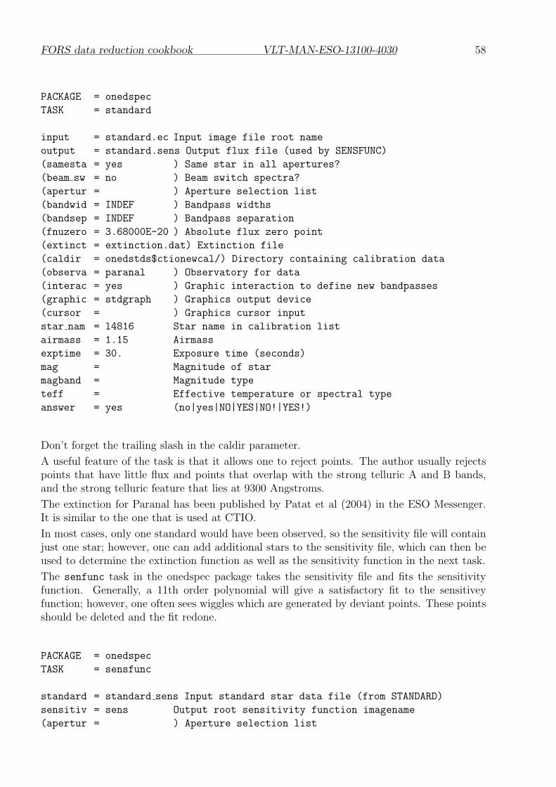
FORS data reduction cookbook VLT-MAN-ESO-13100-4030 58
PACKAGE = onedspec
TASK = standard
input = standard.ec Input image file root name
output = standard.sens Output flux file (used by SENSFUNC)
(samesta = yes ) Same star in all apertures?
(beam sw = no ) Beam switch spectra?
(apertur = ) Aperture selection list
(bandwid = INDEF ) Bandpass widths
(bandsep = INDEF ) Bandpass separation
(fnuzero = 3.68000E-20 ) Absolute flux zero point
(extinct = extinction.dat) Extinction file
(caldir = onedstds$ctionewcal/) Directory containing calibration data
(observa = paranal ) Observatory for data
(interac = yes ) Graphic interaction to define new bandpasses
(graphic = stdgraph ) Graphics output device
(cursor = ) Graphics cursor input
star nam = l4816 Star name in calibration list
airmass = 1.15 Airmass
exptime = 30. Exposure time (seconds)
mag = Magnitude of star
magband = Magnitude type
teff = Effective temperature or spectral type
answer = yes (no|yes|NO|YES|NO!|YES!)
Don’t forget the trailing slash in the caldir parameter.
A useful feature of the task is that it allows one to reject points. The author usually rejectspoints that have little flux and points that overlap with the strong telluric A and B bands,and the strong telluric feature that lies at 9300 Angstroms.
The extinction for Paranal has been published by Patat et al (2004) in the ESO Messenger.It is similar to the one that is used at CTIO.
In most cases, only one standard would have been observed, so the sensitivity file will containjust one star; however, one can add additional stars to the sensitivity file, which can then beused to determine the extinction function as well as the sensitivity function in the next task.
The senfunc task in the onedspec package takes the sensitivity file and fits the sensitivityfunction. Generally, a 11th order polynomial will give a satisfactory fit to the sensitiveyfunction; however, one often sees wiggles which are generated by deviant points. These pointsshould be deleted and the fit redone.
PACKAGE = onedspec
TASK = sensfunc
standard = standard sens Input standard star data file (from STANDARD)
sensitiv = sens Output root sensitivity function imagename
(apertur = ) Aperture selection list

FORS data reduction cookbook VLT-MAN-ESO-13100-4030 59
(ignorea = yes ) Ignore apertures and make one sensitivity functio
(logfile = logfile ) Output log for statistics information
(extinct = extinction.dat) Extinction file
(newexti = ) Output revised extinction file
(observa = paranal ) Observatory of data
(functio = legendre ) Fitting function
(order = 11 ) Order of fit
(interac = yes ) Determine sensitivity function interactively?
(graphs = sr ) Graphs per frame
(marks = plus cross box) Data mark types (marks deleted added)
(colors = 2 1 3 4 ) Colors (lines marks deleted added)
(cursor = ) Graphics cursor input
(device = stdgraph ) Graphics output device
answer = yes (no|yes|NO|YES)
Once the senistivity funciton has been measured, one uses the calibrate task to calibratethe wavelength calibrated spectrum.
PACKAGE = onedspec
TASK = calibrate
input = spectrum.wc spectra to calibrate
output = spectrum.fc Output calibrated spectra
(extinct = yes ) Apply extinction correction?
(flux = yes ) Apply flux calibration?
(extinct = extinction.dat) Extinction file
(observa = paranal ) Observatory of observation
(ignorea = yes ) Ignore aperture numbers in flux calibration?
(sensiti = sens ) Image root name for sensitivity spectra
(fnu = no ) Create spectra having units of FNU?
airmass = 1.1 Airmass
exptime = 900. Exposure time (seconds)
For most people, including the author of these lines, this is good enough. However, thereare additional steps that one might consider. For example, the above steps do not take slitlosses into the acccount, so the spectrum has not been calibrated to an absolute scale. If thewavelength range is very large, then one might have differential slit losses, which means thatthe relative wavelength calibrtion may not be good either. And finally, some people like toremove telluric features, such as the A and B bands, the strong feature at 9300 Angstromsand the weaker features at 7200, 8200 and 9000 Angstroms.

FORS data reduction cookbook VLT-MAN-ESO-13100-4030 60
6 HIgh Time resolution (HIT) modes
Written by Kieran O’Brien, Paranal Science Operations
6.1 Introduction
The HIT modes are specific to FORS2 and for this reason it is important that users understandsome of the basic principles of operation before they plow on ahead and begin to reduce data.Usually this experience comes when the user plans the observations and perhaps even takesthe data themselves. However, this is not always the case, especially in the case of archivaldata analysis. So, with this in mind I will explain a few of the basics and how these affect thesteps needed to calibrate the data.
The general principle of the HIT mode is to increase the duty cycle of imaging and spec-troscopic observations by reducing the exposed region of the CCD and shifting the chargefrom this small region to an unexposed ’storage’ region of the CCD. By shifting the chargein this manner a number of times, it is possible to store a time series of images or spectraon the CCD without needing to read-out the CCD after each exposure. The shutter remainsopen throughout the observation and is only closed once a predefined number of shifts haveoccurred. The CCD is then read-out using the standard low noise read-out mode used for allspectroscopic observations.
t=3
t=4
t=5
t=6
t=7
t=3278
t=3279
t=3280
t=1
t=2
wait = n
wait = n
shift = s
shift = s
Slit Masked region
wait = n
Open shutter
shift = s
wait = n
shift = s
shift = s
Figure 8: The basic operation of the different HIT mode clock patterns. The top panel showsthe clock pattern for the HIT-I and HIT-OS patterns, where each row is shifted individuallyuntil the first row shifted reaches the end of the unvignetted region. The bottom panel showsthe clock pattern for the HIT-MS mode, where a number of rows are grouped together andshifted out from the exposed region into the masked region where they wait for a time whilethe pixels under the slit are exposed to light from the source. ’s’ refers to the size in unbinnedpixels of the slit, whilst ’n’ is the number of seconds to wait between shifts.

FORS data reduction cookbook VLT-MAN-ESO-13100-4030 61
The basic scheme of the HIT-I clock pattern is shown in the top panel of Figure 8. Theimaging mode is available with five variations on this clock pattern. In each the charge isshifted across the unvignetted region of the chip (3280 unbinned pixels) in the direction awayfrom the serial register, but the speed at which the charge is moved is varied to simulate alonger or shorter exposure time. The transfer from t=1-3280 takes place in either 1, 4, 16, 64or 256-seconds, which identifies the clock pattern (ie HIT-OS1-1sec ... HIT-OS5-256sec). Thismeans each row is shifted every 0.61, 2.4, 9.8, 39.0 or 156 milliseconds. The time resolutionof the resulting lightcurve depends on the slit width, as each pixel is exposed as long as itremains in the unmasked region of the CCD. As can be seen in Figure 8 there are also someedge effects if the image of the slit is projected onto more than one pixel.
The HIT-MS mode allows users to operate the CCD with a “shift-and-wait” clock pattern,as shown in the bottom panel of Figure 8. In contrast to the HIT-I and HIT-OS modes,where the charge is constantly being shifted from one row to the next and only the rateat which it is shifted is changed, the HIT-MS clock pattern shifts a pre-defined number ofrows very fast (∼2.5 microseconds per line) and then integrates for a pre-defined ‘wait’ timebefore the sequence is repeated. This continues until the maximum number of line-shifts hasoccurred and the CCD is read-out using the standard low read-out noise spectroscopic mode(100kHz,2x2,high).
6.2 general comments
The first thing to realise with HIT mode data is that there is often a lot of it, well actuallythere is always a LOT of it. For the HIT-MS mode, even if you choose a moderate 1-secondper spectrum, this leads to ∼ 20,000 spectra per night. It is clear from this that you haveto automate the data reduction as much as possible. This means writing scripts. My chosenformat is PERL, as I find it gives me the right degree of flexibility whilst remaining simple tounderstand.
6.3 High time resolution imaging (HIT-I)
6.4 High time resolution spectroscopy (HIT-MS)
The Multiple-Shift (MS) submode of the HIgh-Time resolution (HIT) mode does not behavelike another other mode of FORS and perhaps like any other mode anywhere. However, userswill be relieved to know that, apart from a few peculiarities, it can be treated like a simpleMOS observation. The peculiarity is that instead of the different spectra on a MOS imagerepresenting the spectra of different targets, in the HIT-MS mode they are multiple spectraof the same source (or perhaps sources). In addition, the field is rotated by 90degrees as it isnecessary to have the dispersion parallel to the serial register. I work on each chip separatelyand then combine the 1-D spectra.
6.4.1 Preparation
For data reduction I use the STARLINK software freely available on-line. In addition to this,I use a number of the routines available in PAMELA and MOLLY to work on the 2-D and 1-Dspectra respectively. The reason I chose these packages above more ’mainstream’ ones is thatI have a lot of confidence in the error propagation and they are designed to work in a batch

FORS data reduction cookbook VLT-MAN-ESO-13100-4030 62
Figure 9: An example data-frame taken from chip1 of the data-set used as an example. Thepairs of spectra can be clearly seen. The target spectra are the left-hand spectra, whilst thebrighter comparison star spectra are on the right. Time runs from right to left, as the spectraon the extreme right are the ones that have undergone the most shifts and are therefore thefirst ones taken.
way. In addition, the source code is freely available, easy to follow and sufficiently flexible toallow one to create their own sub-routines and integrate them.
The first stage of the reduction is to convert the files into NDF files that can be understoodby the STARLINK software. For this you should use the fits2ndf task of the convert package.However, the filenames used by ESO contain fullstops, which confuses the software, as it usesthem to mark the beginning of its header structure. The easiest way to avoid this problem isto rename the files as soon as you copy them off the DVD. Once this is done, you can convertthe files
COMMAND: fits2ndf
IN - Input FITS file(s) /@F2hit 0.fits/ >
OUT - Output NDF data structure(s) /@F2hit 0/ >
you should see a lot of files with the extension .sdf. Now we can begin to analyse the data,the first stage as always is to remove the bias level from the frames. In order to do this, I usethe underscan region present on all FORS2 frames. A suitable command to do this in PAMELA
is PICSTAT.
COMMAND: picstat
IMAGE - Input data file /@F2hit 0/ >
STREG - Statistics region input file /’statreg’/ >
CLIP - Sigma rejection threshold /5/ >
PLOT - Do you want histogram plot ? /TRUE/ >
RANGE - Sigma range for plot /5/ >
NBIN - Number of bins /100/ >

FORS data reduction cookbook VLT-MAN-ESO-13100-4030 63
where stat file is a file containing the region (or regions) from which to build the statistic. Anexample of the output of this is
Number of pixels = 189281
Minimum = 172 at X,Y: 164, 837
Maximum = 3669 at X,Y: 142, 66
Straight mean value = 190.942
Straight standard deviation = 12.5663
7 pixels rejected at 5 sigma.
Revised mean value = 190.892
Revised standard deviation = 4.49602
Robust standard deviation = 4.51291
Median value = 191
I use the mean value after sigma-clipping, in this case 190.9 ADU. I then remove this levelfrom the frame using the FIGARO command ICSUB.
COMMAND: icsub
IMAGE - (IMage) Name of image to be subtracted from /@F2hit 0/ >
FACTOR - (FACtor) Constant to be subtracted from image /190.9/ >
OUTPUT - (OUTput) Name of resulting image /@db F2hit 0/ >
The final stage in preparing the data-frames is to edit the headers of the files so that theexposure time for an individual dwell (in this example 2.5 seconds) is parsed to the finalspectra, rather than the total integration time for exposure. This could equally be correctedlater when other parameters are set, but I find it easier to make the correction at this stage.
COMMAND: fitset
FILE - (FIle) Name of file in which FITS keyword is to be
set /@db F2hit 0/ >
KEYWORD - (KEYword) FITS keyword to set or modify /’EXPTIME’/ >
VALUE - (VALue) New value of FITS keyword /’2.5’/ >
COMMENT - (COMment) Comment associated with FITS keyword /’Total
Integration time’/>
6.4.2 Tracing the spectra
Now it is necessary to find the spectra in order to trace the spectral curvature and final extractthe spectrum. In order to do this, I collapse the spectrum over a small number of pixels (soas not to smear the resulting profile too much if it is very curved/tilted) in the dispersiondirection and fit this profile to find the centroid. I use the combination of MEDPRF in PAMELA
and FITGAUSS in FIGARO to do this
COMAND: medprf
IMAGE - Data frame /@db F2hit 0/ >
FLAT - Balance frame /@flat/ >
TRACE - Load a trace of spectrum distortion ? /FALSE/ >
PROFILE - Output profile /@db F2hit 0 gauss/ >
XSTART - Lower X limit /2003/ >

FORS data reduction cookbook VLT-MAN-ESO-13100-4030 64
XEND - Upper X limit /2023/ >
YSTART - Lower Y limit /1/ >
YEND - Upper Y limit /1034/ >
NWIDTH - Median filter width /3/ >
METHOD - L(inear), Q(uadratic) or S(inc) rebinning? /’Q’/ >
where FLAT is the flatfield image and the XSTART, XEND, YSTART, YEND parameters define theregion of interest. The output of this is a file (prof.sdf) containing the spatial profile.
At this point I want to point out that I start extracting spectra at the right-hand side of theimage, as this is the first spectrum taken (i.e. the one that has undergone the most shifts).This makes it a bit easier later on, as the spectrum numbers increase with time, but this isonly my preferred way of doing it.
Secondly, I fit the profile with a Gaussian, in this case non-interactively,
COMMAND: fitgauss
IN - Input NDF /@db F2hit 0 gauss/ >
DEVICE - Graphics device /!/ >
MASK1 - Mask interval lower bound(s) /[2002.5]/ >
MASK2 - Mask interval upper bound(s) /[2022.5]/ >
NCOMP - Number of components /1/ >
CONT - Continuum level /0/ >
CENTRE - Gauss positions /2012.5/ >
PEAK - Gauss heights /800/ >
FWHM - Gauss widths (FWHM) /4/ >
CF - Fit flags for line centres /0/ >
PF - Fit flags for line peaks /0/ >
WF - Fit flags for line widths /0/ >
COMP - Component numbers for storage /1/ >
LOGFIL - ASCII file name for result output /gauss fit/ >
where DEVICE sets the output device name (use ! for no output), MASK1 and MASK2 set thelower and upper spatial limits of the fit respectively, CONT the continuum level, which isalmost certainly negligible in such short exposure times and CENTRE, PEAK and FWHM set theinitial guesses for the fit parameters. You should play around with these in interactive mode(DIALOG=T) a bit before you begin cranking through lots of spectra, as they fitting routine caneasily get lost and give bad results. You can always check these results afterwards to look foroutliers/problems.
Now you can use this information to trace the profile across the columns of the CCD. Tracingthe spectrum is important for the high dispersion VPH grisms, as they are often curved,especially when observing away from the field centre, as we are forced to do with the HITmode in order to try and ’stack’ as many spectra as possible between read-outs. For this Iuse the PAMELA command TRACK. Again, I run it interactively a few times to find good initialparameters before starting the perl-script.
COMMAND: track
IMAGE - Data frame to process /@db F2hit 0/ >
FLAT - Balance frame /@flat/ >

FORS data reduction cookbook VLT-MAN-ESO-13100-4030 65
OLD - Do you want to update an old fit ? /FALSE/ >
TRACK - File for track coefficients /@tr targ/ >
NDPOLY - Order of polynomial fit /4/ >
XSTART - Lower X limit /2003/ >
XEND - Upper X limit /2023/ >
YSTART - Lower Y limit /1/ >
YEND - Upper Y limit /1034/ >
PICK - Pick spectrum point automatically ? /TRUE/ >
NOBJ - Number of objects /1/ >
PLOT - Do you want to plot ? /TRUE/ >
AUTO - Scale frame plot automatically? /TRUE/ >
WIDTH - Width of window /10/ >
ESIG - FWHM of gaussian /3/ >
FWHM - FWHM of profile /3/ >
READOUT - Readout noise (RMS ADU) /4.2/ >
PHOTON - Number of ADU/count /1.43/ >
CLIP - Sigma rejection threshold /3/ >
NBLOCK - Block size /1/ >
TCYCLE - Number of tweak cycles /5/ >
CHANGE - Maximum shift during a tweak /0.5/ >
Figure 10: The output from TRACK. The 2-D spectral profile can clearly be seen. The red-line shows the 4th order polynomial fit to the track. The next spectrum can clearly be seenentering the frame in the top-right. This illustrates that it is essential to extract a ’tracked’spectrum to avoid contamination from nearby spectra.
6.4.3 Extracting the target and sky spectra
Now that we know where the spectrum is and how its position changes across the CCD, weneed to define the different ’regions’ of the spatial profile. These are the spectrum and skyregions that will be used in the subsequent extraction. In order to do this I use the REGPIC

FORS data reduction cookbook VLT-MAN-ESO-13100-4030 66
Figure 11: The resulting fit to the trace from TRACK. This clearly shows that there is a curvatureof 4 pixels across the chip. This example is for the X600B grism and chip1.
command from PAMELA. As the slits are quite short (5”), It is difficult to determine sky regionsthat are sufficiently distant from the target to ensure you are not including flux from the target.Also, it is important to make sure that the sky region does not overlap with the sky regionfrom the comparison star (if one is present), as these will have a different spectrum (andcurvature) due to the offset in the dispersion direction (i.e. the central wavelength falls at adifferent position).
COMMAND: regpic
IMAGE - Data frame /@db F2hit 0/ >
FLAT - Balance frame /@flat/ >
TRACE - Load a trace of spectrum distortion ? /TRUE/ >
TRACK - Distortion map file /@tr targ/ >
REGION - Sky region output file /@targ/ >
GREY - Do you want grey scale plot ? /TRUE/ >
XSTART - Lower X limit /2003/ >
XEND - Upper X limit /2023/ >
YSTART - Lower Y limit /1/ >
YEND - Upper Y limit /1034/ >
AUTO - Do you want automatic choice of scale ? /TRUE/ >
METHOD - Select regions with C(ursor) or T(erminal)? /’T’/ >
Now that you have defined the regions to use as sky, you can extract a 2-dim sky model forthe target region based on polynomial fits to pixel values in the sky regions. I use the PAMELA
command skyfit to do this.
COMMAND: skyfit
IMAGE - Data frame /@db F2hit 0/ >
FLAT - Balance frame /@flat/ >

FORS data reduction cookbook VLT-MAN-ESO-13100-4030 67
Figure 12: The regions selected to represent the sky (dashed red) and target (green) regionsfor the next stage of the extraction.
REGION - Sky region input file /@targ/ >
TRACE - Load a trace of spectrum distortion ? /TRUE/ >
TRACK - Distortion map file /@tr targ/ >
SKY - Sky fit output file /@sky targ/ >
XSTART - Lower X limit /2003/ >
XEND - Upper X limit /2023/ >
YSTART - Lower Y limit /1/ >
YEND - Upper Y limit /1034/ >
NPOLY - Number of terms for the sky fit /3/ > 2
THRESH - Threshold for sky fit /5/ >
READOUT - Readout noise (RMS ADU) /4.2/ >
PHOTON - Detected photons/ADU /1.43/ >
It is important to use a low-order polynomial in this fit, as the spatial extent of the sky regionis small and will not vary very much.
Now we have everything we need to perform the final stage, which is to extract the 1-Dspectrum. The final important decision is how to extract the spectrum. The two choices are’normal’ or ’optimal’ extraction, but you also need to decide whether or not to include thesky fit in the extraction or not. In my experience, the only way to decide these things isto try all the different methods and compare the results. The results depend on a numberof factors, such as the brightness of the object and the atmospheric and sky conditions. Forinstance, unless your sky spectrum contributes a significant fraction to the flux in you extractedtarget spectrum, it is often best not to extract it, as you will only add noise to the extractedspectrum. Likewise, unless your target is faint, it is often not necessary to perform an optimalextraction. However, as I said before, the only way is to try all of the combinations andcompare the results.
COMMAND: extnor
IMAGE - Data frame /@db F2hit 0/ >

FORS data reduction cookbook VLT-MAN-ESO-13100-4030 68
FLAT - Balance factor frame /@flat/ >
REGION - Object region input file /@targ/ >
SKY - Sky fit input file /@sky targ/ >
TRACE - Load a trace of spectrum distortion ? /TRUE/ >
TRACK - Distortion map file /@tr test/ >
SPECT - Spectrum output file /@targ nor/ >
YSTART - Lower Y limit /1/ >
YEND - Upper Y limit /1034/ >
READOUT - Readout noise, RMS data numbers /4.2/ >
PHOTON - Photons/data number /1.43/ >
In the case of optimal extraction, in order to determine the weights for the contributions ofeach pixel to the final spectrum, it is necessary to run the PAMELA command PROFIT.
COMMAND: profit
IMAGE - Data frame /@db F2hit 0/ >
FLAT - Balance factor frame /@unit/ >
REGION - Object region input file /@targ/ >
SKY - Sky fit input file /@sky targ/ >
TRACK - Distortion map file /@tr targ/ >
FRACT - Fraction output file /@targ fract/ >
YSTART - Lower Y limit /1/ >
YEND - Upper Y limit /1034/ >
READOUT - Readout noise, RMS data numbers /4.2/ >
PHOTON - Photons/data number /1.43/ >
NPOLY - Profile poly order /1/ > 5
SIZEX - X separation of polynomials /0.5/ >
THRESH - Rejection threshold /5/ >
NSLOW - Maximum number of one-by-one rejections /10/ >
BADVAL - Bad pixel limit (reject above) /65535/ >
NBLOCK - Wavelength blocking factor /1/ >
NMED - Width of median filter for sums /5/ >
PLOT - Do you want to plot ? /TRUE/ >
This fits polynomials to the flux levels of the columns covered by the target region definedby the REGION file. The polynomials are used to reject outliers caused by cosmics, as thetilt/curvature of the spectrum is assumed to vary smoothly along the columns. The outputfrom this is a 2-D weight map that can is used in the next stage of the PAMELA optimalextraction process. The weight map is used by the command OPTEXT to extract the spectrumof the source. This routine is suitable for curved spectra and should not be confused with theannoyingly similar command EXTOPT, which is only suitable for straight spectra.
COMMAND: OPTEXT
IMAGE - Data frame to process /@db F2hit 0/ >
FLAT - Balance factor frame /@flat/ >
REGION - Object region input file /@targ/ >
SKY - Sky fit input file /@sky targ/ >
TRACK - Distortion map file /@tr targ/ >

FORS data reduction cookbook VLT-MAN-ESO-13100-4030 69
FRACT - Fraction file /@targ fract/ >
SPECT - Spectrum output file /@targ optext/ >
YSTART - Lower Y limit /1/ >
YEND - Upper Y limit /1034/ >
READOUT - Readout noise, RMS data numbers /4.2/ >
PHOTON - Photons/data number /1.43/ >
ZAPRATS - Do you want to reject cosmic rays ? /TRUE/ >
RATLO - Cosmic rat lower rejection threshold /-5/ >
RATHI - Cosmic rat upper rejection threshold /5/ >
EPS - Fudge factor to prevent bad rejections /0.01/ >
PLOT - Do you want to plot ? /TRUE/ >
IAVE - Number of sky rows to average /1/ >
It is important to check the types of events that the code is rejecting, so for the first few times,I would recommend plotting the rejected pixels. This might tell you that the cosmic rejectionthreshold needs to be increased a bit. Once you are happy with the results of the extraction,you need to go back and do everything again for the comparison star. This is necessary, asseveral of the parameters will be quite different for the comparison star due to the differentwavelength coverage compared to the science targets. If you were not able to use a comparisonstar within a few arcseconds of the target, then this difference could be quite large.
6.4.4 fixing the header items
The next step is to update the header items to correct the MJD and integration time. Thefollowing command takes the MJD-OBS keyword from the header and puts it into a file namedhead.file.
hdstrace filename.more nlines=a newline eachline | grep MJD-OBS > head.file
The represents the MJD at the beginning of the exposure, so it is simple to add an integernumber of sub-integration times to this number to give you the MJD of each sub integration.It is then necessary to put this back into the header of the extracted spectrum. It is alsonecessary to include the sub-integration time as the exposure time in a further header itemfor consistency. I use the FIGARO command FITSET to do this. For instance,
COMMAND: FITSET
FILE - (FIle) Name of file /@db F2hit 0/ >
KEYWORD - (KEYword) FITS keyword to set or modify /’EXPTIME’/ >
VALUE - (VALue) New value of FITS keyword /’2.5’/ >
COMMENT - (COMment) Comment associated with keyword /’Integration Time’/ >
In order to ensure that all of the header items are in the correct place, with the correct namesand values, it is necessary to run the perl script (fithead.pl) kindly provided by Tom Marshas part of PAMELA.
Finally, once you have the parameters for the target and comparison star, it is best to startthe automated process. I use the outputs from the previous extraction as the inputs to thenext which assumes that things change smoothly combined with the strict periodicity of theclock pattern to help in determining the centroids of the next target+comparison pair.

FORS data reduction cookbook VLT-MAN-ESO-13100-4030 70
6.4.5 extracting the arcs
Now that you have extracted the science frames, it is necessary to extract the products neededto calibrate the data. The first of these are the arcs, which in the case of FORS, means the arcstaken during the daytime. In the case of the XGRIS 600B, the He and HgCd lamps are used,whereas for the XGRIS 300I, the He and Ar lamps are used. In order to minimize the effectsof the tilt of the spectral trace, I use the trace created from the target and the comparisonstar frames to extract the arc spectra for each of the sub-integrations on the chip. It is notnecessary to use a flatfield for this stage and the sky spectrum should be a zero frame to avoidit misidentifying the arc lines as sky lines. Normal (as opposed to optimal) extraction is bestfor this process, as the S/N is very high.
6.4.6 extracting the flux standard
In order to properly flux calibrate the science frames it is necessary to have two things:
• an observation of a spectro-photometric standard
This is used to calculate the instrumental response for the night. It should be takenwith a slitwidth wide enough to ensure that none of the light is lost
• a ’wide-slit’ observation of the comparison star used in the science observations
This should be taken with the same wide slit as used for the spectro-photometric stan-dard. It is used to measure the losses caused by having the star over-fill the slit. I preferto use the HIT-MS mode to take the data, as it allows me to be confident that nothingelse has changed in the set-up. This might change with time, but it seems to work wellthis way.
The spectra from these frames should be extracted in the same manner as the science, includingthe arc frames taken during the daytime. Now that you have all of the pieces, you can useyour favourite piece of software to wavelength and flux calibrate your data. I use MOLLYfor this, the steps for which can be found on the webpage for the software (http://deneb.astro.warwick.ac.uk/phsaap/software/).

FORS data reduction cookbook VLT-MAN-ESO-13100-4030 71
A Reducing FORS data using the pipeline recipes
A.1 Overview
Since May 21, 2007, the FORS Spectroscopic Pipeline recipes can be downloaded from http:
//www.eso.org/pipelines. The pipeline is currently based on only two recipes, fors calibfor reducing calibration frames and producing an extraction mask, and fors science forapplying the fors calib products to the reduction of scientific exposures. The recipes canbe applied to both FORS1 and FORS2 spectroscopic data obtained in the LSS, MOS, andMXU observation modes. Development work is still ongoing, as these recipes do not yetsupport important tasks such as the combined reduction of jittered scientific exposures, orthe determination of the instrument response curves. Also the reduction of polarimetric andimaging data is not supported yet.
A.2 Launching pipeline recipes: Gasgano and Esorex
Pipeline recipes can be launched using either of two host applications, Gasgano and Esorex.A description about how to use them is given in the FORS Pipeline User’s Manual, that can bedownloaded from http://www.eso.org/pipelines. It is not the purpose of this Cookbook togive a complete description of their usage, but rather to concentrate on data reduction issues.Very briefly, Gasgano is a graphic interface that, besides launching recipes, also helps toclassify and associate the data to be processed; Esorex, on the other hand, is a command lineutility for just launching pipeline recipes: data classification and association must be providedby the user, on the basis of the information attached to the data (e.g., FITS header keywords).The advantage of Esorex is that it may be embedded into scripts for the automation of datareduction tasks.
Each pipeline recipe will process a set of input FITS data files that has been opportunelyselected and classified. To classify an input file means assigning to it an indentification tag,the so-called Data Organiser (DO) category. For instance, a master bias frame is identifiedby the tag MASTER BIAS, and a raw flat field lamp exposure obtained in MOS mode isidentified by the tag SCREEN FLAT MOS. When using Esorex the names of the input filesmust be listed, together with their classification tags, in an ASCII file that is conventionallycalled set-of-frames (SOF). The SOF corresponds to the Input Frames panel of the GasganoRecipe Execution window.
Here is an example of SOF, valid for the fors calib recipe:
../../cal/FORS1_MBIAS.fits MASTER_BIAS
FORS1.2006-05-10T12:58:27.122.fits SCREEN_FLAT_MOS
FORS1.2006-05-10T12:59:45.326.fits SCREEN_FLAT_MOS
FORS1.2006-05-10T13:00:20.930.fits SCREEN_FLAT_MOS
FORS1.2006-05-10T13:01:17.711.fits SCREEN_FLAT_MOS
FORS1.2006-05-10T13:02:14.559.fits SCREEN_FLAT_MOS
FORS1.2006-05-10T13:03:37.926.fits LAMP_MOS
FORS1_ACAT_300I_11_OG590_72.fits MASTER_LINECAT
Each input frame is identified by its path and name, followed by the appropriate classificationtag. Gasgano provides the classification tags automatically.

FORS data reduction cookbook VLT-MAN-ESO-13100-4030 72
In the case of files created by a pipeline recipe, the classification tag is identical to thecontent of the header keyword ESO.PRO.CATG, while for raw files the classification tagis generally based on the content of the keywords ESO.DPR.CATG, ESO.DPR.TYPE, andESO.DPR.TECH (see the FORS Pipeline User’s Manual for more details on the data filesclassification).
Note that the FORS pipeline recipes do not verify in any way the correctness of the classifica-tion tags specified in the SOF: correct tagging must be supplied by external applications, suchas Gasgano or a script provided by the user. A recipe handling an incorrectly tagged filemay stop and display unclear error messages at best. In the worst cases, the recipe would ap-parently run successfully, producing results that may look reasonable, but are actually flawed.
A complete list of the recipes configuration parameters and of their meaning can be found inthe FORS Pipeline User’s Manual. It is also displayed in the Gasgano Recipe Executionwindow, and can be generated by Esorex: for instance, the command
esorex -help fors_calib
would generate a list of the available parameters for recipe fors calib, with their default anda brief explanation of their meaning.
oOo