formulation problem in numerical relativity · d. kramer, et al, exact solutions to einstein’s...
TRANSCRIPT
APCTP Winter School, January 25-26, 2008
Formulation Problem in Numerical RelativityHisaaki Shinkai (Osaka Institute of Technology, Japan)
1. Introduction What is the "Formulation Problem" ?
Historical Review 2. The Standard Approach to Numerical Relativity The ADM formulation
The BSSN formulationHyperbolic formulations
3. Robust system for Constraint Violation Adjusted systems 4. Outlook
http://www.is.oit.ac.jp/~shinkai/
真貝寿明(しんかいひさあき)

APCTP Winter School, January 17-18, 2003 http://home.ewha.ac.kr/~sungwon/school.html

In the last 5 years, ...
Binary BH-BH coalescence simulations are available!!Breakthrough suddenly occurs.
・Pretorius (2005)・Univ. Texas Brownsville (2006)・NASA-Goddard (2006)
Black Hole
Neutron StarNeutron Star
Gravitational Wave
Gravitational Wave
PP oo ss tt -- NN ee ww tt oo nn ii aa nn pp hh aa ss ee
II nn nn ee rr mm oo ss tt SS tt aa bb ll ee CC ii rr cc uu ll aa rr OO rr bb ii tt
CC oo aa ll ee ss cc ee nn cc ee
BB HH FF oo rr mm aa tt ii oo nn
INSP
IRAL
PHA
SE
Newt
onia
n /
Post
-New
toni
an
Inne
rmos
t St
able
Cir
cula
r Or
bit
Po
st-N
ewto
nian
/ G
R
Coal
esce
nce
/ Me
rger
Bl
ack
Hole
For
mati
on
Quas
inor
mal
Ring
ing
Black Hole

In the last 5 years, ...
Binary BH-BH coalescence simulations are available!!
・Pretorius (2005) --> Princeton Univ.・Univ. Texas Brownsville (2006) --> Rochester Univ.・NASA-Goddard (2006)
・Louisiana State Univ. ・Jena Univ.・Pennsylvania State Univ.
"Gold-Rush of parameter searches" (B. Bruegmann, July 2007 @GRG) But ..... Why it works?

Goals of the Lecture
What is the guiding principle for selecting evolution equations for simulations in GR?
Why many groups use the BSSN equations?
Are there an alternative formulation better than the BSSN?
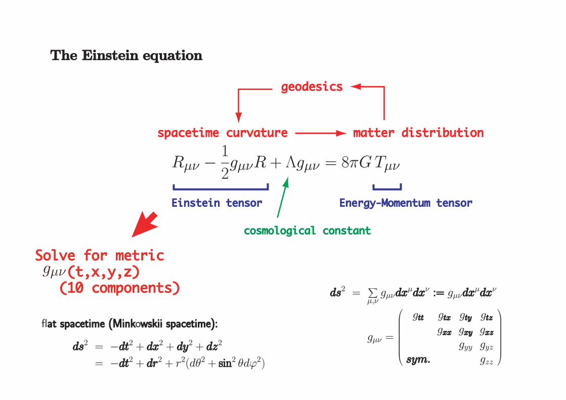
spacetime curvaturespacetime curvature matter distributionmatter distribution
geodesicsgeodesics
Einstein tensorEinstein tensor Energy-Momentum tensorEnergy-Momentum tensor
cosmological constantcosmological constant
Solve for metricSolve for metric (t,x,y,z) (t,x,y,z) (10 components) (10 components)
Rµ! ! 1
2gµ!R + !gµ! = 8"G Tµ!
TheThe EinsteinEinstein equationequation
gµ!
dsds2 =!
µ,!gµ!dxdxµdxdx! :=:= gµ!dxdxµdxdx!
gµ! =
"
########$
gtttt gtxtx gtyty gtztz
gxxxx gxyxy gxzxz
gyy gyz
sysym.m. gzz
%
&&&&&&&&'
flatat spacetimespacetime (Mink(Minkowskiiwskii spacetime):spacetime):
dsds2 = !dtdt2 + dxdx2 + dydy2 + dzdz2
= !dtdt2 + drdr2 + r2(d#2 + sinsin2 #d$2)

The Einstein equation:
Rµν −1
2gµνR + Λgµν = 8πGTµν

The Einstein equation:
Rµν −1
2gµνR + Λgµν = 8πGTµν
Chandrasekhar says ...“Einstein equations are easy to solve. Look at the Exact Solutions book. There aremore than 400 solutions. ”

The Einstein equation:
Rµν −1
2gµνR + Λgµν = 8πGTµν
Chandrasekhar says ...“Einstein equations are easy to solve. Look at the Exact Solutions book. There aremore than 400 solutions. ”
Exact Solutions book says ...1st Edition (1980): “... checked 2000 references, ..., there are now over
100 papers on exact solutions every year, ...”2nd Edition (2003): “... we looked at 4000 new papers published during
1980-1999, ... ”
D. Kramer, et al, Exact Solutions to Einstein’s Field Equations, (Cambridge, 1980)
H. Stephani, et al, Exact Solutions to Einstein’s Field Equations, (Cambridge, 2003)

Why don’t we solve it using computers?
• dynamical behavior, no symmetry in space, ...
• strong gravitational field, gravitational wave! ...
• any dimension, any theories, ...
Numerical Relativity= Solve the Einstein equations numerically.= Necessary for unveiling the nature of strong gravity.
For example:
• gravitational waves from colliding black holes, neutron stars, supernovae, ...
• relativistic phenomena like cosmology, active galactic nuclei, ...
• mathematical feedback to singularity, exact solutions, chaotic behavior, ...
• laboratory for gravitational theories, higher-dimensional models, ...
The most robust way to study the strong gravitational field. Great.

The Einstein equation:
Rµν −1
2gµνR + Λgµν = 8πGTµν
What are the difficulties?
• for 10-component metric, highly nonlinear partial differential equations.mixed with 4 elliptic eqs and 6 dynamical eqs if we apply 3+1 decomposition.
• completely free to choose cooordinates, gauge conditions, and even for decom-position of the space-time.
• has singularity in its nature.
How to solve it?

Numerical Relativity – basic issues HS, APCTP Winter School 2003
0. How to foliate space-time
Cauchy (3 + 1), Hyperboloidal (3 + 1), characteristic (2 + 2), or combined?
⇒ if the foliation is (3 + 1), then · · ·1. How to prepare the initial data
Theoretical: Proper formulation for solving constraints? How to prepare realistic initial data?
Effects of background gravitational waves?Connection to the post-Newtonian approximation?
Numerical: Techniques for solving coupled elliptic equations? Appropriate boundary conditions?
2. How to evolve the data
Theoretical: Free evolution or constrained evolution?Proper formulation for the evolution equations?
Suitable slicing conditions (gauge conditions)?
Numerical: Techniques for solving the evolution equations? Appropriate boundary treatments?Singularity excision techniques? Matter and shock surface treatments?
Parallelization of the code?
3. How to extract the physical information
Theoretical: Gravitational wave extraction? Connection to other approximations?
Numerical: Identification of black hole horizons? Visualization of simulations?

outgoing direction
ingoing direction
S: Initial 2-dimensional Surface
time direction
S: Initial 3-dimensional Surface
First Question: How to foliate space-time?
Cauchy approach or ADM 3+1 formulation
Characteristic approach (if null, dual-null 2+2 formulation)

3+1 versus 2+2
Cauchy (3+1) evolution Characteristic (2+2) evolution
pioneers ADM (1961), York-Smarr (1978) Bondi et al (1962), Sachs (1962),Penrose (1963)
variables easy to understand the concept oftime evolution
has geometrical meanings1 complex function related to 2 GWpolarization modes
foliation has Hamilton structure allows implementation of Penrose’sspace-time compactification
initial data need to solve constraints no constraintsevolution PDEs
need to avoid constraint violationODEs with consistent conditionspropagation eqs along the light rays
singularity need to avoid by some method can truncate the griddisadvantages can not cover space-time globally difficulty in treating caustics
hard to treat matter

“3+1” formulation

Numerical Relativity – basic issues HS, APCTP Winter School 2003
0. How to foliate space-time
Cauchy (3 + 1), Hyperboloidal (3 + 1), characteristic (2 + 2), or combined?
⇒ if the foliation is (3 + 1), then · · ·1. How to prepare the initial data
Theoretical: Proper formulation for solving constraints? How to prepare realistic initial data?
Effects of background gravitational waves?Connection to the post-Newtonian approximation?
Numerical: Techniques for solving coupled elliptic equations? Appropriate boundary conditions?
2. How to evolve the data
Theoretical: Free evolution or constrained evolution?Proper formulation for the evolution equations?
Suitable slicing conditions (gauge conditions)?
Numerical: Techniques for solving the evolution equations? Appropriate boundary treatments?Singularity excision techniques? Matter and shock surface treatments?
Parallelization of the code?
3. How to extract the physical information
Theoretical: Gravitational wave extraction? Connection to other approximations?
Numerical: Identification of black hole horizons? Visualization of simulations?
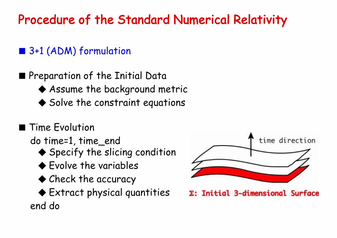
Procedure of the Standard Numerical Relativity
■ 3+1 (ADM) formulation
■ Preparation of the Initial Data◆ Assume the background metric◆ Solve the constraint equations
■ Time Evolutiondo time=1, time_end◆ Specify the slicing condition◆ Evolve the variables◆ Check the accuracy◆ Extract physical quantities
end do

The 3+1 decomposition of space-time: The ADM formulation
[1 ] R. Arnowitt, S. Deser and C.W. Misner, in Gravitation: An Introduction to Current Research,
ed. by L.Witten, (Wiley, New York, 1962).
[2 ] J.W. York, Jr. in Sources of Gravitational Radiation, (Cambridge, 1979)
Dynamics of Space-time = Foliation of Hypersurface
• Evolution of t =const. hypersurface Σ(t).
ds2 = gµνdxµdxν, (µ, ν = 0, 1, 2, 3)
on Σ(t)... dℓ2 = γijdxidxj, (i, j = 1, 2, 3)
• The unit normal vector of the slices, nµ.
nµ = (−α, 0, 0, 0)
nµ = gµνnν = (1/α,−βi/α)
• The lapse function, α. The shift vector, βi.
time direction
Σ: Initial 3-dimensional Surface
ds2 = −α2dt2 + γij(dxi + βidt)(dxj + βjdt)

The decomposed metric:
ds2 = −α2dt2 + γij(dxi + βidt)(dxj + βjdt)
= (−α2 + βlβl)dt2 + 2βidtdxi + γijdxidxj
gµν =
−α2 + βlβl βj
βi γij
, gµν =
−1/α2 βj/α2
βi/α2 γij − βiβj/α2
where α and βj are defined as α ≡ 1/√−g00, βj ≡ g0j.
• The unit normal vector of the slices, nµ.
nµ = (−α, 0, 0, 0)
nµ = gµνnν = (1/α,−βi/α)
• The lapse function, α.
• The shift vector, βi.
coordinate constant linesurface normal line
α dt
βi dt
lapse function, α
shift vector, βi
t = constant hypersurface

Projection of the Einstein equation:
• Projection operator (or intrinsic 3-metric) to Σ(t),
γµν = gµν + nµnν
γµν = δµ
ν + nµnν ≡ ⊥µν
• Define the extrinsic curvature Kij,
Kij ≡ −⊥µi ⊥ν
jnµ;ν
= −(δµi + nµni)(δ
νj + nνnj)nµ;ν
= −ni;j
= Γαijnα = · · · =
1
2α
(
−∂tγij + βi|j + βj|i)
.
• Projection of the Einstein equation:
Gµν nµ nν = 8πG Tµν nµ nν ≡ 8πρH ⇒ the Hamiltonian constraint eq.
Gµν nµ ⊥νi = 8πG Tµν nµ ⊥ν
i ≡ −8πJi ⇒ the momentum constraint eqs.
Gµν ⊥µi ⊥ν
j = 8πG Tµν ⊥µi ⊥ν
j ≡ 8πSij ⇒ the evolution eqs.

The Standard ADM formulation (aka York 1978):The fundamental dynamical variables are (γij,Kij), the three-metric and extrinsiccurvature. The three-hypersurface Σ is foliated with gauge functions, (α, βi), thelapse and shift vector.
• The evolution equations:
∂tγij = −2αKij + Diβj + Djβi,
∂tKij = α (3)Rij + αKKij − 2αKikKkj − DiDjα
+(Diβk)Kkj + (Djβ
k)Kki + βkDkKij
−8πGα{Sij + (1/2)γij(ρH − trS)},where K = Ki
i, and (3)Rij and Di denote three-dimensional Ricci curvature,and a covariant derivative on the three-surface, respectively.
• Constraint equations:
Hamiltonian constr. HADM := (3)R + K2 − KijKij ≈ 0,
momentum constr. MADMi := DjK
ji − DiK ≈ 0,
where (3)R =(3) Rii.

strategy 0 The standard approach :: Arnowitt-Deser-Misner (ADM) formulation (1962)
3+1 decomposition of the spacetime.Evolve 12 variables (!ij, Kij)with a choice of gauge condition.
coordinate constant linesurface normal line
α dt
βi dt
lapse function, α
shift vector, βi
t = constant hypersurface
Maxwell eqs. ADM Einstein eq.
constraintsdiv E = 4"#div B = 0
(3)R + (trK)2 ! KijKij = 2$#H + 2!DjK
ji ! DitrK = $Ji
evolution eqs.
1
c%tE = rot B !
4"
cj
1
c%tB = !rot E
%t!ij = !2NKij + DjNi + DiNj,%tKij = N( (3)Rij + trKKij) ! 2NKilKl
j ! DiDjN+ (DjNm)Kmi + (DiNm)Kmj + NmDmKij ! N!ij!! $&{Sij + 1
2!ij(#H ! trS)}

Procedure of the Standard Numerical Relativity
■ 3+1 (ADM) formulation
■ Preparation of the Initial Data◆ Assume the background metric◆ Solve the constraint equations
■ Time Evolutiondo time=1, time_end◆ Specify the slicing condition◆ Evolve the variables◆ Check the accuracy◆ Extract physical quantities
end do
Need to solve elliptic PDEs -- Conformal approach -- Thin-Sandwich approach
singularity avoidance,simplify the system, GW extraction, ...
Robust formulation ? -- modified ADM / BSSN -- hyperbolization -- asymptotically constrained
Formulation Problem

strategy 0 The standard approach :: Arnowitt-Deser-Misner (ADM) formulation (1962)
3+1 decomposition of the spacetime.
Evolve 12 variables (γij, Kij)
with a choice of gauge condition.coordinate constant line
surface normal line
α dt
βi dt
lapse function, α
shift vector, βi
t = constant hypersurface
Maxwell eqs. ADM Einstein eq.
constraintsdiv E = 4πρ
div B = 0
(3)R + (trK)2 − KijKij = 2κρH + 2Λ
DjKji − DitrK = κJi
evolution eqs.
1
c∂tE = rot B − 4π
cj
1
c∂tB = −rot E
∂tγij = −2NKij + DjNi + DiNj,
∂tKij = N( (3)Rij + trKKij) − 2NKilKlj − DiDjN
+ (DjNm)Kmi + (DiN
m)Kmj + NmDmKij − NγijΛ
− κα{Sij + 12γij(ρH − trS)}

S. Frittelli, Phys. Rev. D55, 5992 (1997)HS and G. Yoneda, Class. Quant. Grav. 19, 1027 (2002)
The Constraint Propagations of the Standard ADM:
!tH = "j(!jH) + 2#KH ! 2#$ij(!iMj)
+#(!l$mk)(2$ml$kj ! $mk$lj)Mj ! 4$ij(!j#)Mi,
!tMi = !(1/2)#(!iH) ! (!i#)H + "j(!jMi)
+#KMi ! "k$jl(!i$lk)Mj + (!i"k)$kjMj.
From these equations, we know that
if the constraints are satisfied on the initial slice !,then the constraints are satisfied throughout evolution (in principle).

Primary / Secondary constraintFirst-class / Second-class constraint
• Primary Constraints
• Secondary Constraints= when propagation of constraints require additional constraints
• First-Class Constraints =

Numerical Relativity in the 20th century1960s Hahn-Lindquist 2 BH head-on collision AnaPhys29(1964)304
May-White spherical grav. collapse PR141(1966)1232
1970s OMurchadha-York conformal approach to initial data PRD10(1974)428Smarr 3+1 formulation PhD thesis (1975)Smarr-Cades-DeWitt-Eppley 2 BH head-on collision PRD14(1976)2443Smarr-York gauge conditions PRD17(1978)2529ed. by L.Smarr “Sources of Grav. Radiation” Cambridge(1979)
1980s Nakamura-Maeda-Miyama-Sasaki axisym. grav. collapse PTP63(1980)1229Miyama axisym. GW collapse PTP65(1981)894Bardeen-Piran axisym. grav. collapse PhysRep96(1983)205Stark-Piran axisym. grav. collapse unpublished
1990 Shapiro-Teukolsky naked singularity formation PRL66(1991)994Oohara-Nakamura 3D post-Newtonian NS coalesence PTP88(1992)307Seidel-Suen BH excision technique PRL69(1992)1845Choptuik critical behaviour PRL70(1993)9NCSA group axisym. 2 BH head-on collision PRL71(1993)2851Cook et al 2 BH initial data PRD47(1993)1471Shibata-Nakao-Nakamura BransDicke GW collapse PRD50(1994)7304Price-Pullin close limit approach PRL72(1994)3297
1995 NCSA group event horizon finder PRL74(1995)630NCSA group hyperbolic formulation PRL75(1995)600Anninos et al close limit vs full numerical PRD52(1995)4462Scheel-Shapiro-Teukolsky BransDicke grav. collapse PRD51(1995)4208Shibata-Nakamura 3D grav. wave collapse PRD52(1995)5428Gunnersen-Shinkai-Maeda ADM to NP CQG12(1995)133Wilson-Mathews NS binary inspiral, prior collapse? PRL75(1995)4161Pittsburgh group Cauchy-characteristic approach PRD54(1996)6153Brandt-Brugmann BH puncture data PRL78(1997)3606Illinois group synchronized NS binary initial data PRL79(1997)1182Shibata-Baumgarte-Shapiro 2 NS inspiral, PN to GR PRD58(1998)023002BH Grand Challenge Alliance characteristic matching PRL80(1998)3915Baumgarte-Shapiro Shibata-Nakamura formulation PRD59(1998)024007Brady-Creighton-Thorne intermediate binary BH PRD58(1998)061501Meudon group irrotational NS binary initial data PRL82(1999)892Shibata 2 NS inspiral coalesence PRD60(1999)104052


Critical Phenomena in Gravitational Collapse Choptuik, Phys. Rev. Lett. 70 (1993) 9
Spherical Sym., Massless Scalar Field (1) scaling (2) echoing (3) universality
Discrite Self-Similarity

Head-on Collision of 2 Black-Holes (Misner initial data)NCSA group 1995

S. Frittelli, Phys. Rev. D55, 5992 (1997)HS and G. Yoneda, Class. Quant. Grav. 19, 1027 (2002)
The Constraint Propagations of the Standard ADM:
!tH = "j(!jH) + 2#KH ! 2#$ij(!iMj)
+#(!l$mk)(2$ml$kj ! $mk$lj)Mj ! 4$ij(!j#)Mi,
!tMi = !(1/2)#(!iH) ! (!i#)H + "j(!jMi)
+#KMi ! "k$jl(!i$lk)Mj + (!i"k)$kjMj.
From these equations, we know that
if the constraints are satisfied on the initial slice !,then the constraints are satisfied throughout evolution (in principle).
But this is NOT TRUE in NUMERICS....

• By the period of 1990s, NR had provided a lot of physics:Gravitational Collapse, Critical Behavior, Naked Singularity, Event Horizons,
Head-on Collision of BH-BH and Gravitational Wavve, Cosmology, · · ·
• However, for the BH-BH/NS-NS inspiral coalescence problem, · · · why ???
Many (too many) trials and errors, hard to find a definit recipe.
time
erro
r
Blow up
t=0
Constrained Surface(satisfies Einstein's constraints)
Best formulation of the Einstein eqs. for long-term stable & accurate simulation?

“Convergence”= higher resolution runs approach to the continuum limit.
(All numerical codes must have this property.)• When the code has 2nd order finite difference scheme, ,
then the error should be scaled with .• “Consistency”, Choptuik, PRD 44 (1991) 3124
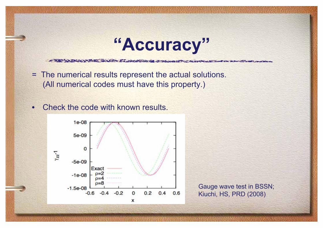
“Accuracy”= The numerical results represent the actual solutions.
(All numerical codes must have this property.)
• Check the code with known results.
Gauge wave test in BSSN;Kiuchi, HS, PRD (2008)


Best formulation of the Einstein eqs. for long-term stable & accurate simulation?
• Many (too many) trials and errors, hard to find a definit recipe.
time
erro
r
Blow up Blow up
ADM
BSSN
Mathematically equivalent formulations, but differ in its stability!
strategy 0: Arnowitt-Deser-Misner (ADM) formulationstrategy 1: Baumgarte-Shapiro-Shibata-Nakamura (BSSN) formulationstrategy 2: Hyperbolic formulationsstrategy 3: “Asymptotically constrained” against a violation of constraints
By adding constraints in RHS, we can kill error-growing modes⇒ How can we understand the features systematically?
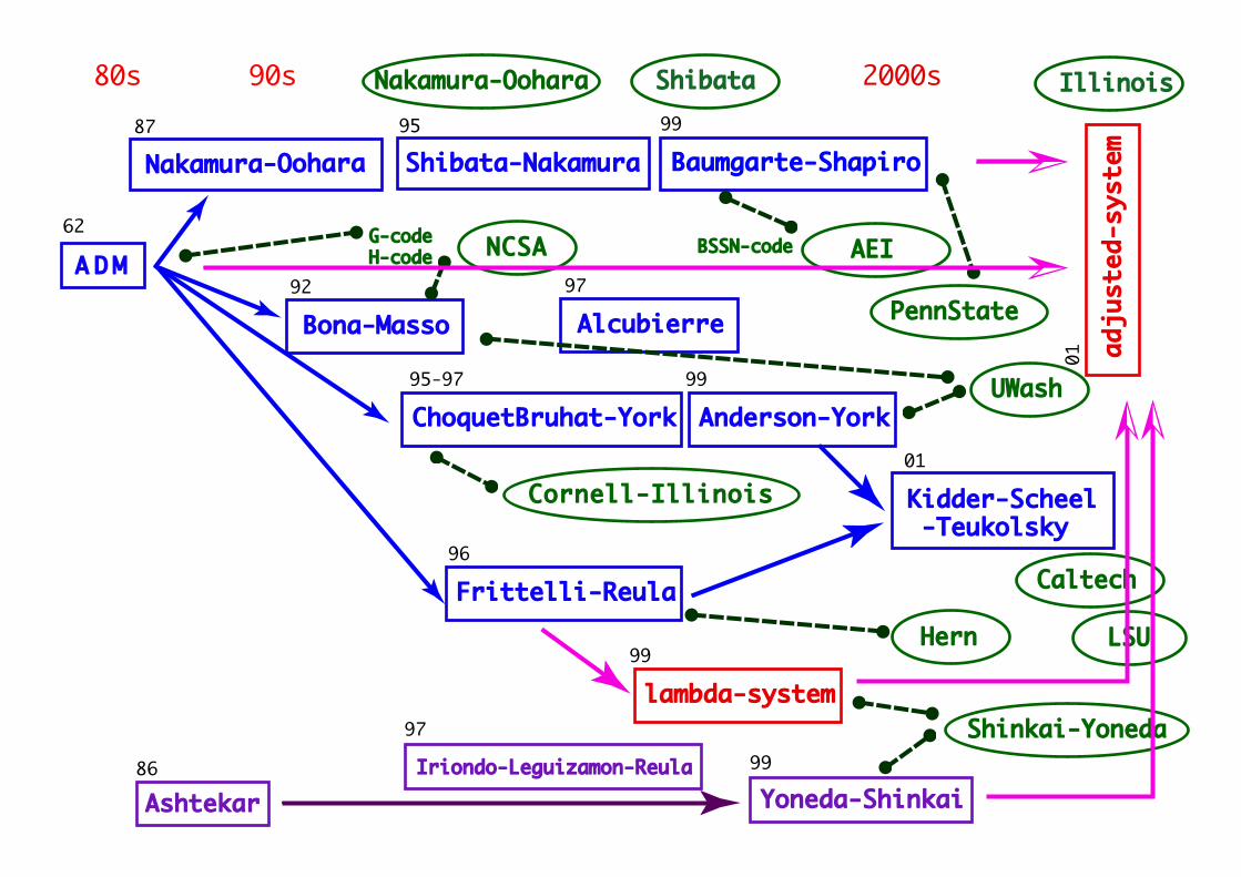
80s 90s 2000s
A D M
Shibata-Nakamura95
Baumgarte-Shapiro99
Nakamura-Oohara87
Bona-Masso92
Anderson-York99
ChoquetBruhat-York95-97
Frittelli-Reula96
62
Ashtekar86
Yoneda-Shinkai99
Kidder-Scheel -Teukolsky
01
lambda-system99
Alcubierre97
Iriondo-Leguizamon-Reula
97

strategy 1 Baumgarte-Shapiro-Shibata-Nakamura (BSSN) formulation
T. Nakamura, K. Oohara and Y. Kojima, Prog. Theor. Phys. Suppl. 90, 1 (1987)
M. Shibata and T. Nakamura, Phys. Rev. D 52, 5428 (1995)
T.W. Baumgarte and S.L. Shapiro, Phys. Rev. D 59, 024007 (1999)
The popular approach. Nakamura’s idea in 1980s.BSSN is a tricky nickname. BS (1999) introduced a paper of SN (1995).
• define new set of variables (φ, γij,K,Aij ,Γi), instead of the ADM’s (γij,Kij) where
γij ≡ e−4φγij, Aij ≡ e−4φ(Kij − (1/3)γijK), Γi ≡ Γijkγ
jk,
and impose detγij = 1 during the evolutions.
• The set of evolution equations become
(∂t − Lβ)φ = −(1/6)αK,
(∂t −Lβ)γij = −2αAij,
(∂t − Lβ)K = αAijAij + (1/3)αK2 − γij(∇i∇jα),
(∂t −Lβ)Aij = −e−4φ(∇i∇jα)TF + e−4φαR(3)ij − e−4φα(1/3)γijR
(3) + α(KAij − 2AikAkj)
∂tΓi = −2(∂jα)Aij − (4/3)α(∂jK)γij + 12αAji(∂jφ) − 2αAk
j(∂jγik) − 2αΓk
ljAjkγ
il
−∂j
(
βk∂kγij − γkj(∂kβ
i) − γki(∂kβj) + (2/3)γij(∂kβ
k))
Momentum constraint was used in Γi-eq.

• Calculate Riemann tensor as
Rij = ∂kΓkij − ∂iΓ
kkj + Γm
ijΓkmk − Γm
kjΓkmi =: Rij + Rφ
ij
Rφij = −2DiDjφ − 2gijD
lDlφ + 4(Diφ)(Djφ) − 4gij(Dlφ)(Dlφ)
Rij = −(1/2)glm∂lmgij + gk(i∂j)Γk + ΓkΓ(ij)k + 2glmΓk
l(iΓj)km + glmΓkimΓklj
• Constraints are H,Mi.
But thre are additional ones, Gi,A,S.
Hamiltonian and the momentum constraint equations
HBSSN = RBSSN + K2 − KijKij, (1)
MBSSNi = MADM
i , (2)
Additionally, we regard the following three as the constraints:
Gi = Γi − γjkΓijk, (3)
A = Aijγij, (4)
S = γ − 1, (5)
Why BSSN better than ADM?Is the BSSN best? Are there any alternatives?
Some known fact (technical):
• Trace-out Aij at every time step helps the stability.Alcubierre, et al, [PRD 62 (2000) 044034]
• “The essential improvement is in the process of replacing terms by the momentumconstraints”,
Alcubierre, et al, [PRD 62 (2000) 124011]
• !i is replaced by !!j"ij where it is not di!erentiated,Campanelli, et al, [PRL96 (2006) 111101; PRD 73 (2006) 061501R]
• !i-equation has been modified as suggested in Yo-Baumgarte-Shapiro [PRD 66(2002) 084026]
Baker et al, [PRL96 (2006) 111102; PRD73 (2006) 104002]
Some guesses:
• BSSN has a wider range of parameters that give us stable evolutions in vonNeumann’s stability analysis. Miller, [gr-qc/0008017]
• The eigenvalues of BSSN evolution equations has fewer “zero eigenvalues” thanthose of ADM, and they conjectured that the instability can be caused by “zeroeigenvalues” that violate “gauge mode”.
M. Alcubierre, et al, [PRD 62 (2000) 124011]

80s 90s 2000s
A D M
Shibata-Nakamura95
Baumgarte-Shapiro99
Nakamura-Oohara87
Bona-Masso92
Anderson-York99
ChoquetBruhat-York95-97
Frittelli-Reula96
62
Ashtekar86
Yoneda-Shinkai99
Kidder-Scheel -Teukolsky
01
lambda-system99
Alcubierre97
Iriondo-Leguizamon-Reula
97

80s 90s 2000s
A D M
Shibata-Nakamura95
Baumgarte-Shapiro99
Nakamura-Oohara87
Bona-Masso92
Anderson-York99
ChoquetBruhat-York95-97
Frittelli-Reula96
62
Ashtekar86
Yoneda-Shinkai99
Kidder-Scheel -Teukolsky
01
NCSA AEIG-code H-code BSSN-code
Cornell-Illinois
UWash
Hern
Caltech
PennState
lambda-system99
Shinkai-Yoneda
Alcubierre97
Nakamura-Oohara Shibata
Iriondo-Leguizamon-Reula
97
LSU
strategy 2 Hyperbolic formulation
Construct a formulation which reveals a hyperbolicity explicitly.For a first order partial differential equations on a vector u,
∂t
u1
u2...
=
A
∂x
u1
u2...
︸ ︷︷ ︸
characteristic part
+ B
u1
u2...
︸ ︷︷ ︸
lower order part
Hyperbolic Formulation(1) Definition
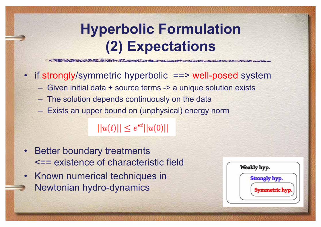
Hyperbolic Formulation(2) Expectations
• if strongly/symmetric hyperbolic ==> well-posed system– Given initial data + source terms -> a unique solution exists– The solution depends continuously on the data– Exists an upper bound on (unphysical) energy norm
• Better boundary treatments<== existence of characteristic field
• Known numerical techniques inNewtonian hydro-dynamics

strategy 2 Hyperbolic formulation
Construct a formulation which reveals a hyperbolicity explicitly.For a first order partial differential equations on a vector u,
∂t
u1
u2...
=
A
∂x
u1
u2...
︸ ︷︷ ︸
characteristic part
+ B
u1
u2...
︸ ︷︷ ︸
lower order part
However,
• ADM is not hyperbolic.
• BSSN is not hyperbolic.
• Many many hyperbolic formulations are presented. Why many? ⇒ Exercise.
One might ask ...
Are they actually helpful?
Which level of hyperbolicity is necessary?

Exercise 1 of hyperbolic formulation Wave equation (∂t∂t − c2∂x∂x)u = 0
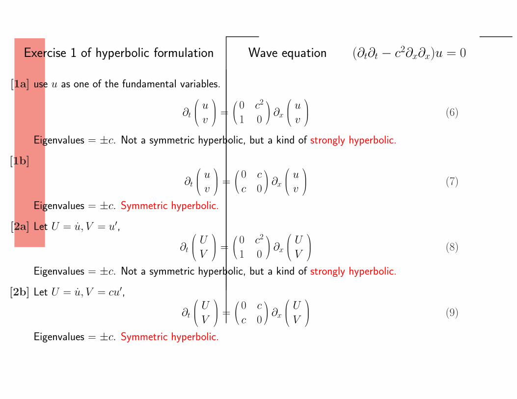
Exercise 1 of hyperbolic formulation Wave equation (∂t∂t − c2∂x∂x)u = 0
[1a] use u as one of the fundamental variables.
∂t
u
v
=
0 c2
1 0
∂x
u
v
(6)
Eigenvalues = ±c. Not a symmetric hyperbolic, but a kind of strongly hyperbolic.
[1b]
∂t
u
v
=
0 c
c 0
∂x
u
v
(7)
Eigenvalues = ±c. Symmetric hyperbolic.
[2a] Let U = u, V = u′,
∂t
U
V
=
0 c2
1 0
∂x
U
V
(8)
Eigenvalues = ±c. Not a symmetric hyperbolic, but a kind of strongly hyperbolic.
[2b] Let U = u, V = cu′,
∂t
U
V
=
0 c
c 0
∂x
U
V
(9)
Eigenvalues = ±c. Symmetric hyperbolic.

Exercise 1 of hyperbolic formulation Wave equation (∂t∂t − c2∂x∂x)u = 0
[3a] Let v = u, w = v′,
∂t
u
v
w
=
0 0 0
0 0 c2
0 1 0
∂x
u
v
w
+
v
0
0
(10)
Eigenvalues = 0,±c. Not a symmetric hyperbolic, nor a strongly hyperbolic.
[3b] Let v = u, w = cv′,
∂t
u
v
w
=
0 0 0
0 0 c
0 c 0
∂x
u
v
w
+
v
0
0
(11)
Eigenvalues = 0,±c. Not a symmetric hyperbolic, nor a strongly hyperbolic.
[4] Let f = u − cu′, g = u + cu′,
∂t
f
g
=
−c 0
0 c
∂x
f
g
(12)
Eigenvalues = ±c. Symmetric hyperbolic, de-coupled.

Exercise 2 of hyperbolic formulation Maxwell equations
Consider the Maxwell equations in the vacuum space,
divE = 0, (1a)
divB = 0, (1b)
rotB − 1
c
∂E
∂t= 0, (1c)
rotE +1
c
∂B
∂t= 0. (1d)

Exercise 2 of hyperbolic formulation Maxwell equations (cont.)
• Take a pair of variables as ui = (E1, E2, E3, B1, B2, B3)T , and write (1c) and
(1d) in the matrix form
∂t
Ei
Bi
∼=
Al ji Bl j
i
C l ji Dl j
i
︸ ︷︷ ︸
Hermitian?
∂l
Ej
Bj
. (2)
• In the Maxwell case, we see immediately
∂tui = c
0 ǫilm
−ǫilm 0
∂lum
or with the actual components
∂t
E1
E2
E3
B1
B2
B3
= c
0
0 −δl3 δl
2
δl3 0 −δl
1
−δl2 δl
1 0
0 δl3 −δl
2
−δl3 0 δl
1
δl2 −δl
1 0
0
∂l
E1
E2
E3
B1
B2
B3
.
That is, symmetric hyperbolic system.

Exercise 2 of hyperbolic formulation Maxwell equations (cont.)
• The eigen-equation of the characteristic matrix becomes
det
Al ji − λlδj
i Bl ji
C l ji Dl j
i − λlδji
= det
−λl 0 00 −λl 00 0 −λl
c
0 −δl3 δl
2
δl3 0 −δl
1
−δl2 δl
1 0
c
0 δl3 −δl
2
−δl3 0 δl
1
δl2 −δl
1 0
−λl 0 00 −λl 00 0 −λl
= 0
We therefore obtain the eigenvalues as
0 (2 multi), ±c√
(δl1)
2 + (δl2)
2 + (δl3)
2 ≡ ±c (2 each)

Exercise 3 of hyperbolic formulation Adjusted Maxwell equations
By adding constraints (1a) and (1b) in the RHS of equations, and see what will behappend.
∂tui = c
0 −ǫilm
ǫilm 0
∂lum + c
xy
∂kEk + c
zw
∂kBk, (3)
where x, y, z, w are parameters.

Exercise 3 of hyperbolic formulation Adjusted Maxwell equations (cont.)
By adding constraints (1a) and (1b) in the RHS of equations, and see what will behappend.
∂tui = c
0 −ǫilm
ǫilm 0
∂lum + c
xy
∂kEk + c
zw
∂kBk, (3)
where x, y, z, w are parameters.
• The actual components are
∂t
E1
E2
E3
B1
B2
B3
= c
x
δl1 δl
2 δl3
δl1 δl
2 δl3
δl1 δl
2 δl3
z
δl1 δl
2 δl3
δl1 δl
2 δl3
δl1 δl
2 δl3
+
0 −δl3 δl
2
δl3 0 −δl
1
−δl2 δl
1 0
y
δl1 δl
2 δl3
δl1 δl
2 δl3
δl1 δl
2 δl3
+
0 δl3 −δl
2
−δl3 0 δl
1
δl2 −δl
1 0
w
δl1 δl
2 δl3
δl1 δl
2 δl3
δl1 δl
2 δl3
∂l
E1
E2
E3
B1
B2
B3
.
We see that adding constraint terms break the symmetricity of the characteristicmatrix.
• The eigenvalues will be changed asc
2
(
x + w ±√
x2 − 2xw + w2 + 4yz)
(δl1 + δl
2 + δl3) (1 each), ±c (2 each).
The zero eigenvalues disappear by adding constraints, and they can be also |c| ifthe parameters have the relation (yz − xw − 1)2 = (x + w)2.

80s 90s 2000s
A D M
Shibata-Nakamura95
Baumgarte-Shapiro99
Nakamura-Oohara87
Bona-Masso92
Anderson-York99
ChoquetBruhat-York95-97
Frittelli-Reula96
62
Ashtekar86
Yoneda-Shinkai99
Kidder-Scheel -Teukolsky
01
NCSA AEIG-code H-code BSSN-code
Cornell-Illinois
UWash
Hern
Caltech
PennState
lambda-system99
Shinkai-Yoneda
Alcubierre97
Nakamura-Oohara Shibata
Iriondo-Leguizamon-Reula
97
LSU
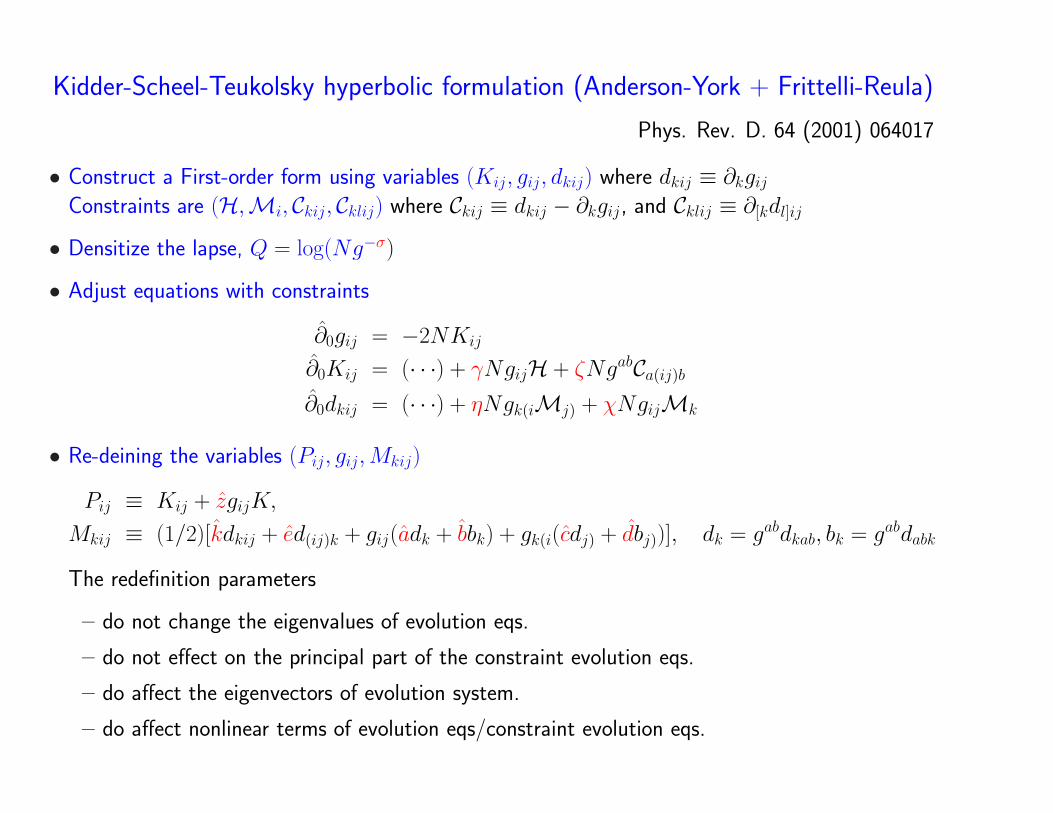
Kidder-Scheel-Teukolsky hyperbolic formulation (Anderson-York + Frittelli-Reula)
Phys. Rev. D. 64 (2001) 064017
• Construct a First-order form using variables (Kij, gij, dkij) where dkij ≡ ∂kgij
Constraints are (H,Mi, Ckij, Cklij) where Ckij ≡ dkij − ∂kgij, and Cklij ≡ ∂[kdl]ij
• Densitize the lapse, Q = log(Ng−σ)
• Adjust equations with constraints
∂0gij = −2NKij
∂0Kij = (· · ·) + γNgijH + ζNgabCa(ij)b
∂0dkij = (· · ·) + ηNgk(iMj) + χNgijMk
• Re-deining the variables (Pij, gij, Mkij)
Pij ≡ Kij + zgijK,
Mkij ≡ (1/2)[kdkij + ed(ij)k + gij(adk + bbk) + gk(i(cdj) + dbj))], dk = gabdkab, bk = gabdabk
The redefinition parameters
– do not change the eigenvalues of evolution eqs.
– do not effect on the principal part of the constraint evolution eqs.
– do affect the eigenvectors of evolution system.
– do affect nonlinear terms of evolution eqs/constraint evolution eqs.

Numerical experiments of KST hyperbolic formulation
Weak wave on flat spacetime.-> No non-principal part.
-> We can observe the features of hyperbolicity.
-> Using constraints in RHS may improve the blow-up.
Stability properties of a formulation of Einstein’s equations
Gioel Calabrese,* Jorge Pullin,† Olivier Sarbach,‡ and Manuel Tiglio§
Department of Physics and Astronomy, Louisiana State University, 202 Nicholson Hall, Baton Rouge, Louisiana 70803-4001
!Received 27 May 2002; published 19 September 2002"
We study the stability properties of the Kidder-Scheel-Teukolsky !KST" many-parameter formulation ofEinstein’s equations for weak gravitational waves on flat space-time from a continuum and numerical point of
view. At the continuum, performing a linearized analysis of the equations around flat space-time, it turns out
that they have, essentially, no non-principal terms. As a consequence, in the weak field limit the stability
properties of this formulation depend only on the level of hyperbolicity of the system. At the discrete level we
present some simple one-dimensional simulations using the KST family. The goal is to analyze the type of
instabilities that appear as one changes parameter values in the formulation. Lessons learned in this analysis
can be applied in other formulations with similar properties.
DOI: 10.1103/PhysRevD.66.064011 PACS number!s": 04.25.Dm
I. INTRODUCTION
Numerical simulations of the Einstein equations for situ-
ations of interest in the binary black hole problem do not run
forever. The codes either stop due to the development offloating point overflows, or even if they do not crash, theyproduce answers that after a while are clearly incorrect. It isusually very difficult to pinpoint a clear reason why a codestops working. Recently, Kidder, Scheel and Teukolsky!KST" #1$ introduced a twelve-parameter family of evolutionequations for general relativity. Performing an empirical pa-rameter study within a certain two-parameter subfamily, theywere able to evolve single black hole space-times for over1000 M, where M is the mass of the black hole, somethingthat had been very difficult to achieve in the past. It is ofinterest to try to understand what makes some of the param-eter choices better than others, in particular given that atwelve dimensional parameter study appears prohibitive atpresent. The intention of this paper is to take some steps inthis direction. We will first perform a linearized analysis ofthe KST equations in the continuum, by considering smallperturbations around flat space-time. We will observe that thestability of flat space-time is entirely characterized by thelevel of hyperbolicity of the system. Since the latter is con-trolled by the parameters of the family, this provides a firstanalytic guidance as to which values to choose. Unfortu-nately, the result is somewhat weak, since it just points to anobvious fact: formulations with a higher level of hyperbolic-ity work better.In the second part of the paper we perform a set of simple
numerical tests. We consider space-times where all variablesdepend on one spatial coordinate, which we consider com-pactified for simplicity, and time. We are able to exhibit ex-plicitly the various types of instabilities that arise in the sys-tem. Some of the results are surprising. For the situationwhere the system is weakly hyperbolic, the code is strictly
nonconvergent, but it might appear to converge for a signifi-cant range of resolutions. We will see that the addition ofdissipation does not fix these problems, but actually can ex-acerbate them. It is often the case in numerical relativity thatdiscretization schemes that are convergent for strongly hy-perbolic equations are applied to weakly hyperbolic formu-lations. The examples of this section will teach us how dan-gerous such a practice is and confirm the analytic results ofRef. #2$. This part of the paper is also instructive in that theKST system has only been evolved with pseudospectralmethods. We use ordinary integration via the method oflines.The plan of this paper is as follows. In the next section we
will discuss several notions of stability that are present in theliterature, mostly to clarify the notation. In Sec. III we dis-cuss the stability of the KST equations in the continuumunder linearized perturbations. In Sec. IV we discuss the nu-merical simulations.
II. DIFFERENT DEFINITIONS OF STABILITY
The term stability is used in numerical relativity in severaldifferent ways. We therefore wanted to make the notationclear at least in what refers to this paper. Sometimes thenotion of stability is used in a purely analytic context, whilesome other times it is used in a purely numerical one. Withinanalytical contexts, there are cases in which it is used tomean well posedness, as in the book of Kreiss and Lorenz#3$. In such a context well posedness means that the norm ofthe solution at a fixed time can be bounded by the norm ofthe initial data, with a bound that is valid for all initial data.In other cases it is intended to measure the growth of pertur-bations of a certain solution within a formulation of Ein-stein’s equations, without special interest in whether theequations are well posed or not.At the numerical level, a scheme is sometimes defined as
stable if it satisfies a discrete version of well posedness. Thisis the sense in which stability !plus consistency" is equivalentto convergence via the Lax theorem #4$. Examples of thiskind of instability are present in the Euler scheme, schemeswith Courant factor that are too large, or other situationswhere the amplification factor !or its generalization" is big-
*Electronic address: [email protected]†Electronic address: [email protected]‡Electronic address: [email protected]§Electronic address: [email protected]
PHYSICAL REVIEW D 66, 064011 !2002"
0556-2821/2002/66!6"/064011!12"/$20.00 ©2002 The American Physical Society66 064011-1
lutions the coarsest one gives smaller errors after a while,
and the time at which this occurs decreases as one increases
resolution. This indicates that the difference scheme is not
convergent. Note that one could be easily misled to think that
the code is convergent if one did not evolve the system for
long enough time, or without high enough resolution. For
example, if one performs two runs, with 120 and 240 grid-
points, one has to evolve until, roughly, 150 crossing times,
in order to notice the lack of convergence. To put these num-
bers in context, suppose one had a similar situation in a 3D
black hole evolution. To give some usual numbers, suppose
the singularity is excised, with the inner boundary at, say, r
!M , and the outer boundary is at 20M !which is quite amodest value if one wants to extract waveforms". In this case120 and 240 gridpoints correspond to grid spacings of, ap-
proximately, M /5 and M /10, respectively !usual values aswell in some simulations". If one had to evolve up to 150crossing times in order to notice the lack of convergence,
that would correspond to t!3000M , which is several timesmore than what present 3D evolutions last. Of course, the
situation presented in this simple example need not appear in
exactly the same way in an evolution of a different space-
time, or with a different discretization; in fact, in the next
subsection we show an example where the instability be-
comes obvious sooner. Also, there are some ways of noticing
in advance that the code is not converging. Namely, it seems
that the numerical solution has the expected power law
growth that the continuum linearized analysis predicts until
all of a sudden an exponential growth appears. But if one
looks at the Fourier components of the numerical solution,
one finds that there are nonzero components growing expo-
nentially from the very beginning, starting at the order of
truncation error !see Fig. 8".One might expect that, since for WH systems the
frequency-dependent growth at the continuum is a power law
one, it is possible to get convergence by adjusting the dissi-
pation. In #2$ we show that even though certain amount of
dissipation might help, the code is never convergent and,
indeed, adding too much dissipation violates the von Neu-
mann condition, which leads to a much more severe numeri-
cal instability. We have systematically done numerical ex-
periments changing the value of % without being able to
stabilize the simulations !more details are given below", veri-fying, thus, the discrete predictions.
3. The CIP case (!ÄÀ1Õ2)
Figure 9 shows the error in the metric, for different reso-
lutions. As in the WH case, the errors originate mostly from
the nonzero frequencies !i.e. the ones that typically grow inan unstable numerical scheme". But now they grow more
than 10 orders of magnitude in much less than one crossing
time and it is quite obvious that the code is not converging.
This is so because in the CIP case the instability grows ex-
ponentially with the number of gridpoints !see Fig. 10". Thiscan be seen performing a discrete analysis for the single ill
posed equation in 1D, v t!ivx . One gets that the symbol&('(x) is real and cannot be bounded by 1 in magnitude,making the difference scheme unstable !independently ofresolution". If one changed to characteristic variables exactlythis equation would appear in 1D as a subset of the system
that we are considering, so this model equation is, in the
FIG. 7. L2 norms of the errors for the metric. FIG. 8. Fourier components of the numerical metric for )!0,4,8. Some of the components grow exponentially from the verybeginning.
FIG. 9. L2 norm of the errors for the metric.
CALABRESE, PULLIN, SARBACH, AND TIGLIO PHYSICAL REVIEW D 66, 064011 !2002"
064011-8
reaches the value !!0.32 the instability is even worse thanadding less dissipation, and the same thing happens if one
keeps on increasing ! beyond 0.32. So we next narrow the
interval in which the dissipation is fine tuned, we start at !!0.24, and increase at intervals of 0.01. We find the same
result; at !"0.25 there is already too much dissipation and
the situation is worse. Fine tuning even more, we change !in intervals of 0.001 around 0.250, but it is also found that
for !"0.250 the effect of more dissipation is adverse, asalso shown in Fig. 14.
The fact that beyond !!0.250 the situation becomesworse is in perfect agreement with the discrete analysis of
"2#. There we show that a necessary condition for the von
Neumann condition to be satisfied is !$%1/8. Here the up-per limit of 1/8 corresponds to, precisely, !!1/4. Exceedingthis value results in a violation of the von Neumann condi-
tion; as explained in "2#, when this happens there is a nu-merical instability that grows exponentially with the number
of gridpoints &i.e. as in the CIP case', much faster than when
the von Neumann condition is satisfied &in which case thegrowth goes as a power of the gridpoints'.Finally, it is worthwhile to point out that we have also
tried with smaller Courant factors, using, in particular, values
often used in numerical relativity, like $!0.20 and $!0.25, without ever being able to get a completely conver-gent simulation.
3. The CIP case
Finally here we also use the parameters &21' with (!1,but now we take )!#79/42, which implies $2!#1 and,thus, the system is CIP. The results are as expected. There is
exponential, frequency-dependent growth that makes the nu-
merical scheme unstable, see Fig. 15.
C. Other simulations
Performing simulations with the ICN instead of the RK
method yields similar results, as predicted in "2#. Figure 16shows, for example, evolutions changing the densitization of
the lapse, as in the first subsection, but using the ICN method
with two iterations &counting this number as in "9#'. This isthe minimum number of iterations that yields a stable
scheme for well posed equations but, as shown in "2#, it isunstable for WH systems. The same values of the Courant
factor and dissipation as above were used in these runs. We
have also tried with other values of the Courant factor and
dissipation parameter, finding similar results. We were able
to confirm the lack of convergence predicted in "2# in everyWH or CIP formulation we used, including the ADM equa-
tions rewritten as first order equations in time space. Lack of
convergence with a 3D code, using the ADM equations writ-
ten as second order in space and the ICN method, for the
same initial data used here, has also been confirmed "10#.
V. DISCUSSION
We have shown that a linearized analysis of the KST
equations implies that flat space-time written in Cartesian
coordinates is a stable solution of the equations if the param-
FIG. 11. Amplification factor associated with the difference
scheme &12' approximating the ill posed equation v t!ivx .
FIG. 12. L2 norm of the errors for the metric.
FIG. 13. L2 norm of the errors for the metric. The simulation is
stopped once the determinant of the spatial metric becomes zero.
CALABRESE, PULLIN, SARBACH, AND TIGLIO PHYSICAL REVIEW D 66, 064011 &2002'
064011-10

Class. Quantum Grav. 17 (2000) 4799–4822. Printed in the UK PII: S0264-9381(00)50711-4
Hyperbolic formulations and numerical relativity:experiments using Ashtekar’s connection variables
Hisa-aki Shinkai† and Gen Yoneda‡† Centre for Gravitational Physics and Geometry, 104 Davey Laboratory, Department of Physics,The Pennsylvania State University, University Park, PA 16802-6300, USA‡ Department of Mathematical Sciences, Waseda University, Shinjuku, Tokyo, 169-8555, Japan
E-mail: [email protected] and [email protected]
Received 3 May 2000, in final form 13 September 2000
Abstract. In order to perform accurate and stable long-time numerical integration of the Einsteinequation, several hyperbolic systems have been proposed. Here we present a numerical comparisonbetween weakly hyperbolic, strongly hyperbolic and symmetric hyperbolic systems based onAshtekar’s connection variables. The primary advantage for using this connection formulation inthis experiment is that we can keep using the same dynamical variables for all levels of hyperbolicity.Our numerical code demonstrates gravitational wave propagation in plane-symmetric spacetimes,and we compare the accuracy of the simulation by monitoring the violation of the constraints.By comparing with results obtained from the weakly hyperbolic system, we observe that thestrongly and symmetric hyperbolic system show better numerical performance (yield less constraintviolation), but not so much difference between the latter two. Rather, we find that the symmetrichyperbolic system is not always the best in terms of numerical performance.
This study is the first to present full numerical simulations using Ashtekar’s variables. Wealso describe our procedures in detail.
(Some figures in this article are in colour only in the electronic version; see www.iop.org)
PACS numbers: 0420C, 0425, 0425D
1. Introduction
Numerical relativity—solving the Einstein equation numerically—is now an essential field ingravity research. As is well known, critical collapse in gravity systems was first discovered bynumerical simulation [1]. The current mainstream of numerical relativity is to demonstrate thefinal phase of compact binary objects related to gravitational wave observations†, and theseefforts are now again shedding light on the mathematical structure of the Einstein equations.
Up to a couple of years ago, the standard Arnowitt–Deser–Misner (ADM) decompositionof the Einstein equation was taken as the standard formulation for numerical relativists.Difficulties in accurate/stable long-term evolutions were supposed to be overcome by choosingproper gauge conditions and boundary conditions. Recently, however, several numericalexperiments show that the standard ADM is not the best formulation for numerics, and findinga better formulation has become one of the main research topics‡.
† The latest reviews are available in [2].‡ Note that we are only concerned with the free evolution system of the initial data; that is, we only solve the constraintequations on the initial hypersurface. The accuracy and/or stability of the system is normally observed by monitoringthe violation of constraints during the free evolution.
0264-9381/00/234799+24$30.00 © 2000 IOP Publishing Ltd 4799
Hyperbolic formulations and numerical relativity 4803
N˜, Ni, Aa
0, which we call the densitized lapse function, shift vector and the triad lapse function.The system has three constraint equations,
CASHH := (i/2)!ab
c EiaE
jbF c
ij ! 0, (7)
CASHMi := "Fa
ij Eja ! 0, (8)
CASHGa := Di E
ia ! 0, (9)
which are called the Hamiltonian, momentum and Gauss constraint equations, respectively.The dynamical equations for a set of (Ei
a, Aai ) are
"t Eia = "iDj (!
cbaN˜Ej
c Eib) + 2Dj (N
[j Ei]a ) + iAb
0!abc Ei
c, (10)
"tAai = "i!ab
cN˜E
jbF c
ij + NjF aji + DiAa
0, (11)
where Faij := 2"[iAa
j ] " i!abc Ab
i Acj is the curvature 2-form.
We have to consider the reality conditions when we use this formalism to describe theclassical Lorentzian spacetime. As we review in appendix A.2, the metric will remain on itsreal-valued constraint surface during time evolution automatically if we prepare initial datawhich satisfy the reality condition. More practically, we also require that the triad be real-valued. However, again this reality condition appears as a gauge restriction on Aa
0, (A11),which can be imposed at every time step. In our actual simulation, we prepare our initial datausing the standard ADM approach, so that we have no difficulties in maintaining these realityconditions.
The set of dynamical equations (10) and (11) (hereafter we call these the original equations)does have a weakly hyperbolic form [19], so that we regard the mathematical structure ofthe original equations as one step advanced from the standard ADM. Furthermore, we canconstruct higher levels of hyperbolic systems by restricting the gauge condition and/or byadding constraint terms, CASH
H , CASHMi and CASH
Ga , to the original equations [19]. We extract onlythe final expressions here.
In order to obtain a symmetric hyperbolic system†, we add constraint terms to the right-hand side of (10) and (11). The adjusted dynamical equations,
"t Eia = "iDj (!
cbaN˜Ej
c Eib) + 2Dj (N
[j Ei]a ) + iAb
0!abc Ei
c + P iab CASH
Gb, (12)
where
P iab # Ni#ab + iN
˜!ab
cEic,
"tAai = "i!ab
cN˜E
jbF c
ij + NjF aji + DiAa
0 + Qai C
ASHH + Ri
ja CASHMj , (13)
where
Qai # e"2N
˜Ea
i , Rija # ie"2N
˜!ac
bEbi E
jc
form a symmetric hyperbolicity if we further require the gauge conditions,
Aa0 = Aa
i Ni, "iN = 0. (14)
We note that the adjusted coefficients, P iab, Q
ai , Ri
ja , for constructing the symmetrichyperbolic system are uniquely determined, and there are no other additional terms (say,no CASH
H , CASHM for "t E
ia , no CASH
G for "tAai ) [19]. The gauge conditions, (14), are consequences
of the consistency with (triad) reality conditions.
† Iriondo et al [34] presented a symmetric hyperbolic expression in a different form. The differences between oursand theirs are discussed in [19, 20]
Hyperbolic formulations and numerical relativity 4811
Figure 2. Images of gravitational wave propagation and comparisons of dynamical behaviour ofAshtekar’s variables and ADM variables. We applied the same initial data of two +-mode pulsewaves (a = 0.2, b = 2.0, c = ±2.5 in equation (21) and K0 = !0.025), and the same slicingcondition, the standard geodesic slicing condition (N = 1). (a) Image of the 3-metric componentgyy of a function of proper time ! and coordinate x. This behaviour can be seen identically bothin ADM and Ashtekar evolutions, and both with the Brailovskaya and Crank–Nicholson time-integration scheme. Part (b) explains this fact by comparing the snapshot of gyy at the same propertime slice (! = 10), where four lines at ! = 10 are looked at identically. Parts (c) and (d) are of thereal part of the densitized triad E
y2 , and the real part of the connection A2
y , respectively, obtainedfrom the evolution of the Ashtekar variables.
When the pulses collide, then the amplitude seems simply to double, as they are superposed,and the pulses keep travelling in their original propagation direction. That is, we observesomething like solitonic wave pulse propagation.
As we mentioned in section 3.2, we have to assume our background not to be flat, thereforethere are no exact solutions. The reader might think that if we set | tr K| to be small and pulsewave shapes to be quite sharp then our simulations will be close to the analytic collidingplane-wave solutions which produce the curvature singularity. However, from the numericalside, these two requirements are contradictory (e.g. sharp wave input produces large curvaturewhich should be compensated by | tr K| in order to construct our initial data). Thus it is notso surprising that our waves propagate like solitons, not forming a singularity.
In figure 2(a), we plot an image of wave propagation (a metric component gyy) up to! = 10, of +-mode pulse waves initially located at x = ±2.5. We took a small negative K0,so that the background spacetime is slowly expanding.
Figure 2(b), then, tells us that our ADM evolution code and Ashtekar’s variable code giveus identical evolutions. We plotted a snapshot of gyy on the initial data (which is common toall models here), and its snapshot at ! = 10.0. The fact that all four lines (ADM/Ashtekar, of

No drastic differences in stabilitybetween 3 levels of hyperbolicity.
Class. Quantum Grav. 17 (2000) 4799–4822. Printed in the UK PII: S0264-9381(00)50711-4
Hyperbolic formulations and numerical relativity:experiments using Ashtekar’s connection variables
Hisa-aki Shinkai† and Gen Yoneda‡† Centre for Gravitational Physics and Geometry, 104 Davey Laboratory, Department of Physics,The Pennsylvania State University, University Park, PA 16802-6300, USA‡ Department of Mathematical Sciences, Waseda University, Shinjuku, Tokyo, 169-8555, Japan
E-mail: [email protected] and [email protected]
Received 3 May 2000, in final form 13 September 2000
Abstract. In order to perform accurate and stable long-time numerical integration of the Einsteinequation, several hyperbolic systems have been proposed. Here we present a numerical comparisonbetween weakly hyperbolic, strongly hyperbolic and symmetric hyperbolic systems based onAshtekar’s connection variables. The primary advantage for using this connection formulation inthis experiment is that we can keep using the same dynamical variables for all levels of hyperbolicity.Our numerical code demonstrates gravitational wave propagation in plane-symmetric spacetimes,and we compare the accuracy of the simulation by monitoring the violation of the constraints.By comparing with results obtained from the weakly hyperbolic system, we observe that thestrongly and symmetric hyperbolic system show better numerical performance (yield less constraintviolation), but not so much difference between the latter two. Rather, we find that the symmetrichyperbolic system is not always the best in terms of numerical performance.
This study is the first to present full numerical simulations using Ashtekar’s variables. Wealso describe our procedures in detail.
(Some figures in this article are in colour only in the electronic version; see www.iop.org)
PACS numbers: 0420C, 0425, 0425D
1. Introduction
Numerical relativity—solving the Einstein equation numerically—is now an essential field ingravity research. As is well known, critical collapse in gravity systems was first discovered bynumerical simulation [1]. The current mainstream of numerical relativity is to demonstrate thefinal phase of compact binary objects related to gravitational wave observations†, and theseefforts are now again shedding light on the mathematical structure of the Einstein equations.
Up to a couple of years ago, the standard Arnowitt–Deser–Misner (ADM) decompositionof the Einstein equation was taken as the standard formulation for numerical relativists.Difficulties in accurate/stable long-term evolutions were supposed to be overcome by choosingproper gauge conditions and boundary conditions. Recently, however, several numericalexperiments show that the standard ADM is not the best formulation for numerics, and findinga better formulation has become one of the main research topics‡.
† The latest reviews are available in [2].‡ Note that we are only concerned with the free evolution system of the initial data; that is, we only solve the constraintequations on the initial hypersurface. The accuracy and/or stability of the system is normally observed by monitoringthe violation of constraints during the free evolution.
0264-9381/00/234799+24$30.00 © 2000 IOP Publishing Ltd 4799
4816 H Shinkai and G Yoneda
Figure 6. Comparisons of the ‘adjusted’ system with the different multiplier, ! , in equations (31)and (32). The model uses +-mode pulse waves (a = 0.1, b = 2.0, c = ±2.5) in equation (21) in abackground K0 = !0.025. Plots are of the L2 norm of the Hamiltonian and momentum constraintequations, CASH
H and CASHM ((a) and (b), respectively). We see some ! produce a better performance
than the symmetric hyperbolic system.
Our numerical code demonstrates gravitational wave propagation in plane-symmetricspacetime, and we compare the ‘accuracy’ and/or ‘stability’ by monitoring the violation ofthe constraints. Actually, our experiments in section 4 were the comparisons of accuracyin evolutions, while in section 5 we observed cases of unstable evolution. By comparingwith the results obtained from the weakly hyperbolic system, we observe that the stronglyand symmetric hyperbolic system show better properties with little differences between them.Therefore, we may conclude that higher levels of hyperbolic formulations help the numericsmore, though the differences are small.
However, we also found that the symmetric hyperbolic system is not always the bestone for controlling accuracy or stability, by introducing a multiplier for adjusted terms inthe equations of motion. This result suggests that a certain kind of hyperbolicity is enoughto control the violation of the constraint equation. In our case it is the strongly hyperbolic
Hyperbolic formulations and numerical relativity 4815
5. Experiments 2: another way to control the accuracy/stability
The results we have presented in the previous section indicate that both strongly and symmetrichyperbolic systems show better performance than the original weakly hyperbolic system.These systems are obtained by adding constraint terms (or ‘adjusted’ terms) to the right-handside of the original equations, (10) and (11). In this section, we report on simple experimentsin changing the magnitude of the multipliers of such adjusted terms.
We consider the following system, where the equations of motion are adjusted in the sameway as before, but with a real-valued constant multiplier !:
"t Eia = !iDj (#
cbaN˜Ej
c Eib) + 2Dj (N
[j Ei]a ) + iAb
0#abc Ei
c + !P iab CASH
Gb, (31)
where P iab " Ni$ab + iN
˜#ab
cEic,
"tAai = !i#ab
cN˜E
jbF c
ij + NjF aji + DiAa
0 + !Qai C
ASHH + !Ri
ja CASHMj , (32)
where Qai " e!2N
˜Ea
i , Rija " ie!2N
˜#ac
bEbi E
jc .
The set of equations (31) and (32) becomes the original weakly hyperbolic system if ! = 0,becomes the symmetric hyperbolic system if ! = 1 and N = constant, and remains a stronglyhyperbolic system for other choices of ! except ! = 1
2 which only forms a weakly hyperbolicsystem. We again remark that the coefficients for constructing the symmetric hyperbolicsystem are uniquely determined.
We tried the same evolutions as in the previous section for different value of ! . In figure 6,we plot the L2 norm of the Hamiltonian and momentum constraint equations, CASH
H and CASHM .
We checked first that ! = 0 and 1 produce the same results as those of weakly and symmetrichyperbolic systems. What is interesting is the case of ! = 2 and 3. These !s producebetter performance than the symmetric hyperbolic system, although these cases are of stronglyhyperbolic levels. Therefore, as far as monitoring the violation of the constraints is concerned,we may say that the symmetric hyperbolic form is not always the best. We note that thenegative ! will produce unstable evolution as we plotted, while too a large positive ! will alsoresult in unstable evolution in the end (see the ! = 3 lines).
We also tried similar experiments with the vacuum Maxwell equation. The originalMaxwell equation has a symmetric hyperbolicity, and additional constraint terms (withmultiplier !) reduce the hyperbolicity to the strong or weak level. We show the details and afigure in appendix B, but in short there may be no measurable differences between stronglyand symmetric hyperbolicities.
These experiments in changing ! are now reported in our paper II [41] more extensively.There, we propose a plausible explanation as to why such adjusted terms work for stabilizingthe system. We introduce the idea in appendix C. Briefly, we will conjecture a criterion usingthe eigenvalues of the ‘adjusted version’ of the constraint propagation equations. This analysismay explain the appearance of phase differences between two systems, which is observed infigures 4–6.
6. Discussion
Motivated by many recent proposals for hyperbolic formulations of the Einstein equation, westudied numerically these accuracy/stability properties with the purpose of comparing threemathematical levels of hyperbolicity: weakly hyperbolic, strongly hyperbolic and symmetrichyperbolic systems. We apply Ashtekar’s connection formulation, because this is the onlyknown system in which we can compare three hyperbolic levels with the same interface.

BSSN Pros:
• With Bona-Masso-type # (1+log), and frozon $ (!t!i " 0), BSSN plus auxiliaryvariables form a 1st-order symmetric hyperbolic system,
Heyer-Sarbach, [PRD 70 (2004) 104004]
• If we define 2nd order symmetric hyperbolic form, principal part of BSSN can beone of them,
Gundlach-MartinGarcia, [PRD 70 (2004) 044031, PRD 74 (2006) 024016]
BSSN Cons:
• Existence of an ill-posed solution in BSSN (as well in ADM)Frittelli-Gomez [JMP 41 (2000) 5535]
• Gauge shocks in Bona-Masso slicing is inevitable. Current 3D BH simulation islack of resolution.
Garfinke-Gundlach-Hilditch [arXiv:0707.0726]

strategy 2 Hyperbolic formulation (cont.)
Are they actually helpful?
“YES” group
“Well-posed!”, ||u(t)|| ≤ eκt||u(0)||
Mathematically Rigorous Proofs
IBVP in future

Initial Boundary Value Problem
GR-IBVPStewart, CQG15 (98) 2865
Tetrad formalismFriedrich & Nagy, CMP201 (99) 619
Linearized Bianchi eq.Buchman & Sarbach, CQG 23 (06) 6709
Constraint-preserving BCKreiss, Reula, Sarbach & Winicour, CQG 24 (07) 5973
Higher-order absorbing BCRuiz, Rinne & Sarbach, CQG 24 (07) 6349
Consistent treatment is availableonly for symmetric hyperbolicsystems.

strategy 2 Hyperbolic formulation (cont.)
Are they actually helpful?
“YES” group “Really?” group
“Well-posed!”, ||u(t)|| ≤ eκt||u(0)|| “not converging”, still blow-up
Mathematically Rigorous Proofs Proofs are only simple eqs.Discuss only characteristic part.Ignore non-principal part.
IBVP in future...
Which level of hyperbolicity is necessary?
symmetric hyperbolic ⊂ strongly hyperbolic ⊂ weakly hyperbolic systems,
Advantages in Numerics (90s)
Advantages in sym. hyp.– KST formulation by LSU

strategy 2 Hyperbolic formulation (cont.)
Are they actually helpful?
“YES” group “Really?” group
“Well-posed!”, ||u(t)|| ≤ eκt||u(0)|| “not converging”, still blow-up
Mathematically Rigorous Proofs Proofs are only simple eqs.Discuss only characteristic part.Ignore non-principal part.
IBVP in future...
Which level of hyperbolicity is necessary?
symmetric hyperbolic ⊂ strongly hyperbolic ⊂ weakly hyperbolic systems,
Advantages in Numerics (90s) These were vs. ADM
Advantages in sym. hyp.– KST formulation by LSU
Not much differences in hyperbolic 3 levels– FR formulation, by Hern– Ashtekar formulation, by HS-Yoneda
sym. hyp. is not always the best

80s 90s 2000s
A D M
Shibata-Nakamura95
Baumgarte-Shapiro99
Nakamura-Oohara87
Bona-Masso92
Anderson-York99
ChoquetBruhat-York95-97
Frittelli-Reula96
62
Ashtekar86
Yoneda-Shinkai99
Kidder-Scheel -Teukolsky
01
NCSA AEIG-code H-code BSSN-code
Cornell-Illinois
UWash
Hern
Caltech
PennState
lambda-system99
Shinkai-Yoneda
Alcubierre97
Nakamura-Oohara Shibata
Iriondo-Leguizamon-Reula
97
LSU
80s 90s 2000s
A D M
Shibata-Nakamura95
Baumgarte-Shapiro99
Nakamura-Oohara87
Bona-Masso92
Anderson-York99
ChoquetBruhat-York95-97
Frittelli-Reula96
62
Ashtekar86
Yoneda-Shinkai99
Kidder-Scheel -Teukolsky
01
NCSA AEIG-code H-code BSSN-code
Cornell-Illinois
UWash
Hern
Caltech
PennState
lambda-system99
adju
sted
-sys
tem
01
Shinkai-Yoneda
Alcubierre97
Nakamura-Oohara Shibata
Iriondo-Leguizamon-Reula
97
LSU
Illinois

Summary up to here (1st half)
[Keyword 1] Formulation Problem Although mathematically equivalent, different set of equations
shows different numerical stability.
[Keyword 2] ADM formulationThe starting formulation (Historically & Numerically). Successes in 90s, but not for binary BH-BH/NS-NS problems.
[Keyword 3] BSSN formulationNew variables and gauge fixing to ADM, shows better stability. The reason why it is better was not known at first.Many simulation groups uses BSSN. Technical tips are accumulated.
[Keyword 4] hyperbolic formulationsMathematical classification of PDE shows "well-posedness", but its meaning is limited. Many versions of hyperbolic Einstein equations are available. Some group try to show the advantage of BSSN using "hyperbolicity".But are they really helpful in numerics?
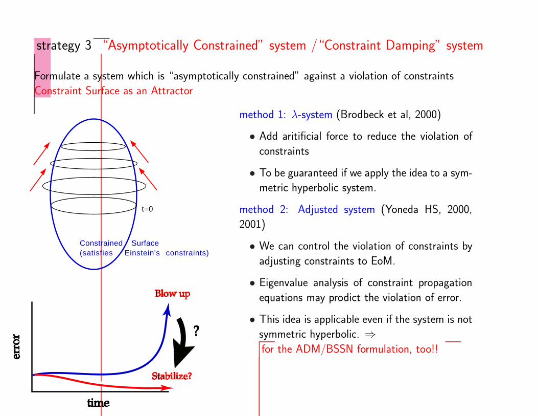
strategy 3 “Asymptotically Constrained” system /“Constraint Damping” system
Formulate a system which is “asymptotically constrained” against a violation of constraints
Constraint Surface as an Attractor
t=0
Constrained Surface(satisfies Einstein's constraints)
time
erro
r
Blow up
Stabilize?
?
method 1: λ-system (Brodbeck et al, 2000)
• Add aritificial force to reduce the violation of
constraints
• To be guaranteed if we apply the idea to a sym-
metric hyperbolic system.
method 2: Adjusted system (Yoneda HS, 2000,
2001)
• We can control the violation of constraints by
adjusting constraints to EoM.
• Eigenvalue analysis of constraint propagation
equations may prodict the violation of error.
• This idea is applicable even if the system is not
symmetric hyperbolic. ⇒for the ADM/BSSN formulation, too!!
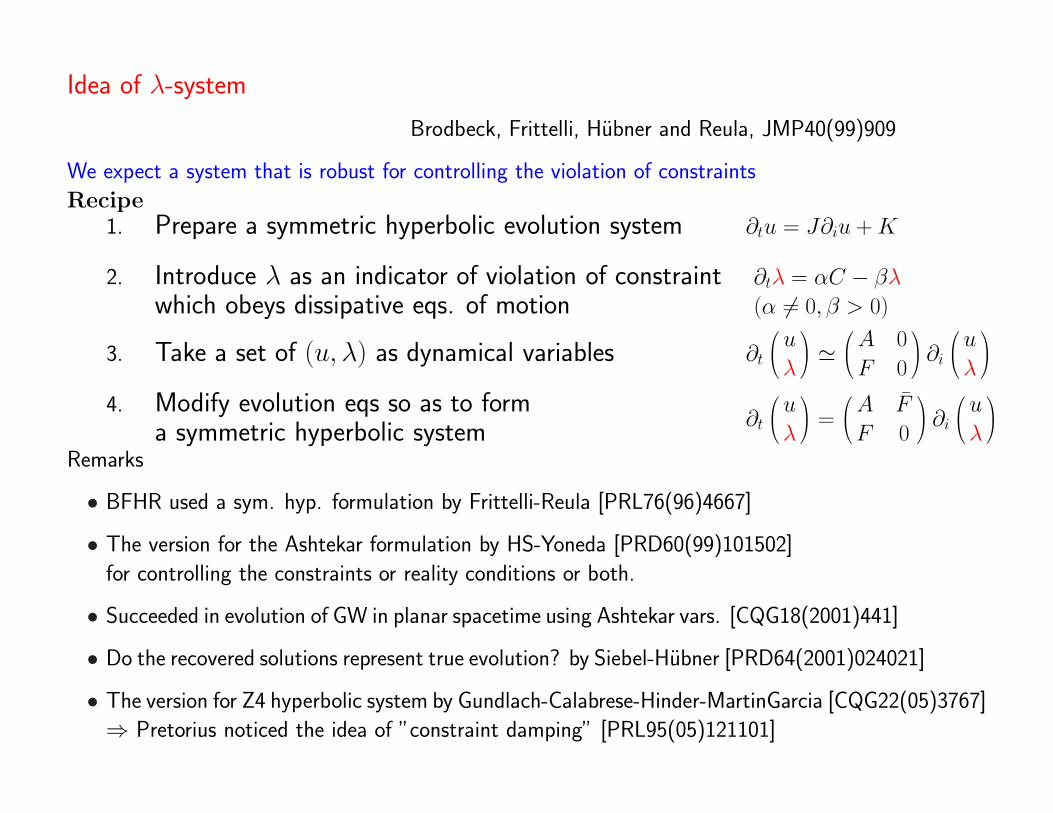
Idea of λ-system
Brodbeck, Frittelli, Hubner and Reula, JMP40(99)909
We expect a system that is robust for controlling the violation of constraints
Recipe1. Prepare a symmetric hyperbolic evolution system ∂tu = J∂iu + K
2. Introduce λ as an indicator of violation of constraintwhich obeys dissipative eqs. of motion
∂tλ = αC − βλ
(α 6= 0, β > 0)
3. Take a set of (u, λ) as dynamical variables ∂t
u
λ
≃
A 0
F 0
∂i
u
λ
4. Modify evolution eqs so as to forma symmetric hyperbolic system
∂t
u
λ
=
A F
F 0
∂i
u
λ
Remarks
• BFHR used a sym. hyp. formulation by Frittelli-Reula [PRL76(96)4667]
• The version for the Ashtekar formulation by HS-Yoneda [PRD60(99)101502]
for controlling the constraints or reality conditions or both.
• Succeeded in evolution of GW in planar spacetime using Ashtekar vars. [CQG18(2001)441]
• Do the recovered solutions represent true evolution? by Siebel-Hubner [PRD64(2001)024021]
• The version for Z4 hyperbolic system by Gundlach-Calabrese-Hinder-MartinGarcia [CQG22(05)3767]
⇒ Pretorius noticed the idea of ”constraint damping” [PRL95(05)121101]

Maxwell-lambda system works as expected.
Hyperbolic formulations and numerical relativity: II 445
with the initial data !E = !B = 0 and take (E, B, !E, !B) as a set of variables to evolve:
"t
!
"
"
"
#
Ei
Bi
!E
!B
$
%
%
%
&
=
!
"
"
"
#
0 !c#ijl 0 0
c#ijl 0 0 0
$1%lj 0 0 0
0 $2%lj 0 0
$
%
%
%
&
"l
!
"
"
"
#
Ej
Bj
!E
!B
$
%
%
%
&
+
!
"
"
"
#
0
0
!&1!E
!&2!B
$
%
%
%
&
. (2.14)
We immediately obtain an expected symmetric form as
"t
!
"
"
"
#
Ei
Bi
!E
!B
$
%
%
%
&
=
!
"
"
"
#
0 !c#ijl $1%
li 0
c#ijl 0 0 $2%
li
$1%lj 0 0 0
0 $2%lj 0 0
$
%
%
%
&
"l
!
"
"
"
#
Ej
Bj
!E
!B
$
%
%
%
&
+
!
"
"
"
#
0
0
!&1!E
!&2!B
$
%
%
%
&
. (2.15)
2.2.2. Analysis of eigenvalues. Now the evolution equations for the constraints CE and CB
become
"tCE = $1('!E), "tCB = $2('!B) (2.16)
where ' = "i"i . We take the Fourier integrals for constraints Cs (2.16) and !s, (2.12) and
(2.13), in the form of (2.7), to obtain
"t
!
"
"
"
#
CE
CB
!E
!B
$
%
%
%
&
=
!
"
"
"
#
0 0 !$1k2 0
0 0 0 !$2k2
$1 0 !&1 0
0 $2 0 !&2
$
%
%
%
&
!
"
"
"
#
CE
CB
!E
!B
$
%
%
%
&
, (2.17)
where k2 = kiki . We find the matrix to be constant. Note that this is an exact expression.
Since the eigenvalues are'
!&1 ±(
&21 ! 4$2
1k2)
/2
and'
!&2 ±(
&22 ! 4$2
2k2)
/2,
the negative eigenvalue requirement becomes $1, $2 "= 0 and &1, &2 > 0.
2.2.3. Numerical demonstration. We present a numerical demonstration of the aboveMaxwell ‘! system’. We prepare a code which produces electromagnetic propagation inthe xy-plane, and monitor the violation of the constraint during time integration. Specifically,we prepare the initial data with a Gaussian packet at the origin,
Ei(x, y, z) =*
!Ay e!B(x2+y2), Ax e!B(x2+y2), 0+
, (2.18)
Bi(x, y, z) = (0, 0, 0), (2.19)
where A and B are constants, and let it propagate freely, under the periodic boundarycondition.
The code itself is quite stable for this problem. In figure 1, we plot the L2 norm of theerror (CE over the whole grid) as a function of time. The full curve (constant) in figure 1(a)is of the original Maxwell equation. If we introduce !s, then we see that the error will bereduced by a particular choice of $ and &. Figure 1(a) is for changing $ with & = 2.0,
446 G Yoneda and H Shinkai
Figure 1. Demonstration of the ! system in the Maxwell equation. (a) Constraint violation (L2norm of CE ) versus time with constant " (= 2.0) but changing #. Here # = 0 means no ! system.(b) The same plot with constant # (= 0.5) but changing ". We see better performance for " > 0,which is the case of negative eigenvalues of the constraint propagation equation. The constants in(2.18) were chosen as A = 200 and B = 1.
INSTITUTE OF PHYSICS PUBLISHING CLASSICAL AND QUANTUM GRAVITY
Class. Quantum Grav. 18 (2001) 441–462 www.iop.org/Journals/cq PII: S0264-9381(01)15923-X
Hyperbolic formulations and numerical relativity: II.asymptotically constrained systems of Einsteinequations
Gen Yoneda1 and Hisa-aki Shinkai2
1 Department of Mathematical Sciences, Waseda University, Shinjuku, Tokyo, 169-8555, Japan2 Centre for Gravitational Physics and Geometry, 104 Davey Lab., Department of Physics, ThePennsylvania State University, University Park, PA 16802-6300, USA
E-mail: [email protected] and [email protected]
Received 27 July 2000, in final form 13 December 2000
AbstractWe study asymptotically constrained systems for numerical integration of theEinstein equations, which are intended to be robust against perturbative errorsfor the free evolution of the initial data. First, we examine the previouslyproposed ‘! system’, which introduces artificial flows to constraint surfacesbased on the symmetric hyperbolic formulation. We show that this systemworks as expected for the wave propagation problem in the Maxwell systemand in general relativity using Ashtekar’s connection formulation. Second, wepropose a new mechanism to control the stability, which we call the ‘adjustedsystem’. This is simply obtained by adding constraint terms in the dynamicalequations and adjusting their multipliers. We explain why a particular choiceof multiplier reduces the numerical errors from non-positive or pure-imaginaryeigenvalues of the adjusted constraint propagation equations. This ‘adjustedsystem’ is also tested in the Maxwell system and in the Ashtekar system. Thismechanism affects more than the system’s symmetric hyperbolicity.
PACS numbers: 0420C, 0425, 0425D
(Some figures in this article are in colour only in the electronic version; see www.iop.org)
1. Introduction
Numerical relativity, an approach to solving the Einstein equations numerically, is supposedto be the only way to study highly nonlinear gravitational phenomena. Although the attemptalready has decades of history, we still do not have a definite recipe for integrating the Einsteinequations that will give us accurate and long-term stable time evolutions. Here and hereafter,we mean by ‘stable evolution’ that the system keeps the violation of the constraints within asuitable small value in its free numerical evolution.
0264-9381/01/030441+22$30.00 © 2001 IOP Publishing Ltd Printed in the UK 441

Ashtekar-lambda system works as expected, as well.
INSTITUTE OF PHYSICS PUBLISHING CLASSICAL AND QUANTUM GRAVITY
Class. Quantum Grav. 18 (2001) 441–462 www.iop.org/Journals/cq PII: S0264-9381(01)15923-X
Hyperbolic formulations and numerical relativity: II.asymptotically constrained systems of Einsteinequations
Gen Yoneda1 and Hisa-aki Shinkai2
1 Department of Mathematical Sciences, Waseda University, Shinjuku, Tokyo, 169-8555, Japan2 Centre for Gravitational Physics and Geometry, 104 Davey Lab., Department of Physics, ThePennsylvania State University, University Park, PA 16802-6300, USA
E-mail: [email protected] and [email protected]
Received 27 July 2000, in final form 13 December 2000
AbstractWe study asymptotically constrained systems for numerical integration of theEinstein equations, which are intended to be robust against perturbative errorsfor the free evolution of the initial data. First, we examine the previouslyproposed ‘! system’, which introduces artificial flows to constraint surfacesbased on the symmetric hyperbolic formulation. We show that this systemworks as expected for the wave propagation problem in the Maxwell systemand in general relativity using Ashtekar’s connection formulation. Second, wepropose a new mechanism to control the stability, which we call the ‘adjustedsystem’. This is simply obtained by adding constraint terms in the dynamicalequations and adjusting their multipliers. We explain why a particular choiceof multiplier reduces the numerical errors from non-positive or pure-imaginaryeigenvalues of the adjusted constraint propagation equations. This ‘adjustedsystem’ is also tested in the Maxwell system and in the Ashtekar system. Thismechanism affects more than the system’s symmetric hyperbolicity.
PACS numbers: 0420C, 0425, 0425D
(Some figures in this article are in colour only in the electronic version; see www.iop.org)
1. Introduction
Numerical relativity, an approach to solving the Einstein equations numerically, is supposedto be the only way to study highly nonlinear gravitational phenomena. Although the attemptalready has decades of history, we still do not have a definite recipe for integrating the Einsteinequations that will give us accurate and long-term stable time evolutions. Here and hereafter,we mean by ‘stable evolution’ that the system keeps the violation of the constraints within asuitable small value in its free numerical evolution.
0264-9381/01/030441+22$30.00 © 2001 IOP Publishing Ltd Printed in the UK 441
448 G Yoneda and H Shinkai
We introduce new variables (!, !i , !a), obeying the dissipative evolution equations,
"t! = #1 CH ! $1 !, (2.26)
"t!i = #2 CMi ! $2 !i , (2.27)
"t!a = #3 CGa ! $3 !a, (2.28)
where #i "= 0 (possibly complex) and $i > 0 (real) are constants.If we take y# := (Ei
a, Aai , !, !i , !a) as a set of dynamical variables, then the principal
part of (2.26)–(2.28) can be written as
"t!#= !i#1%
bcdEjc El
d ("lAbj ), (2.29)
"t!i#= #2[!e&l
i Ejb + e&
ji E
lb]("lAb
j ), (2.30)
"t!a#= #3"l E
la. (2.31)
The characteristic matrix of the system u# is not Hermitian. However, if we modifythe right-hand side of the evolution equation of (Ei
a, Aai ), then the set becomes a symmetric
hyperbolic system. This is done by adding #3'il("l!a) to the equation of "t E
ia , and by adding
i#1%acdEc
i Eld ("l!)+ #2(!e' lmEa
i +e&mi Ela)("l!m) to the equation of "tAa
i . The final principalpart is then written as
"t
!
"
"
"
"
#
Eia
Aai
!
!i
!a
$
%
%
%
%
&
#=
!
"
"
"
"
"
"
#
Mlabi
j 0 0 0 #3'il&a
b
0 N l ai b
j i#1%acdEc
i Eld #2e(&
ji E
la ! ' lj Eai ) 0
0 !i#1%bcdE
jc El
d 0 0 0
0 #2e(&ji E
lb ! &l
i Ejb ) 0 0 0
#3&ba&
lj 0 0 0 0
$
%
%
%
%
%
%
&
$"l
!
"
"
"
"
#
Ejb
Abj
!
!j
!b
$
%
%
%
%
&
, (2.32)
where
Mlabij = i%abcN#El
c'ij + Nl' ij&ab, (2.33)
N labij = iN#(%abcEj
c ' li ! %abcElc'
ji ! e!2Eia%bcdEjc El
d ! e!2%acdEid E
lcE
jb
+e!2%acdEid E
jc Elb) + Nl&ab' ij . (2.34)
Clearly, the solution (Eia, Aa
i , !, !i , !a) = (Eia, Aa
i , 0, 0, 0) represents the originalsolution of the Ashtekar system.
Hyperbolic formulations and numerical relativity: II 451
Figure 3. Demonstration of the ! system in the Ashtekar equation. We plot the violation of theconstraint (the L2 norm of the Hamiltonian constraint equation, CH ) for the cases of plane-wavepropagation under the periodic boundary. To see the effect more clearly, we added an artificial errorat t = 6. Part (a) shows how the system goes bad depending on the amplitude of artificial error.The error was of the form A2
y ! A2y(1 + error). All the curves are of the evolution of Ashtekar’s
original equation (no ! system). Part (b) shows the effect of the ! system. All the curves have20% error amplitude, but show the difference of the evolution equations. The full curve is forAshtekar’s original equation (the same as in (a)), the dotted curve is for the strongly hyperbolicAshtekar equation. Other curves are of ! systems, which produce a better performance than thatof the strongly hyperbolic system.

Idea of “Adjusted system” and Our Conjecture
CQG18 (2001) 441, PRD 63 (2001) 120419, CQG 19 (2002) 1027
General Procedure
1. prepare a set of evolution eqs. ∂tua = f(ua, ∂bu
a, · · ·)
2. add constraints in RHS ∂tua = f(ua, ∂bu
a, · · ·) +F (Ca, ∂bCa, · · ·)
︸ ︷︷ ︸
3. choose appropriate F (Ca, ∂bCa, · · ·)
to make the system stable evolution
How to specify F (Ca, ∂bCa, · · ·) ?
4. prepare constraint propagation eqs. ∂tCa = g(Ca, ∂bC
a, · · ·)
5. and its adjusted version ∂tCa = g(Ca, ∂bC
a, · · ·) +G(Ca, ∂bCa, · · ·)
︸ ︷︷ ︸
6. Fourier transform and evaluate eigenvalues ∂tCk = A(Ca)
︸ ︷︷ ︸
Ck
Conjecture: Evaluate eigenvalues of (Fourier-transformed) constraint propagation eqs.
If their (1) real part is non-positive, or (2) imaginary part is non-zero, then the system is more stable.
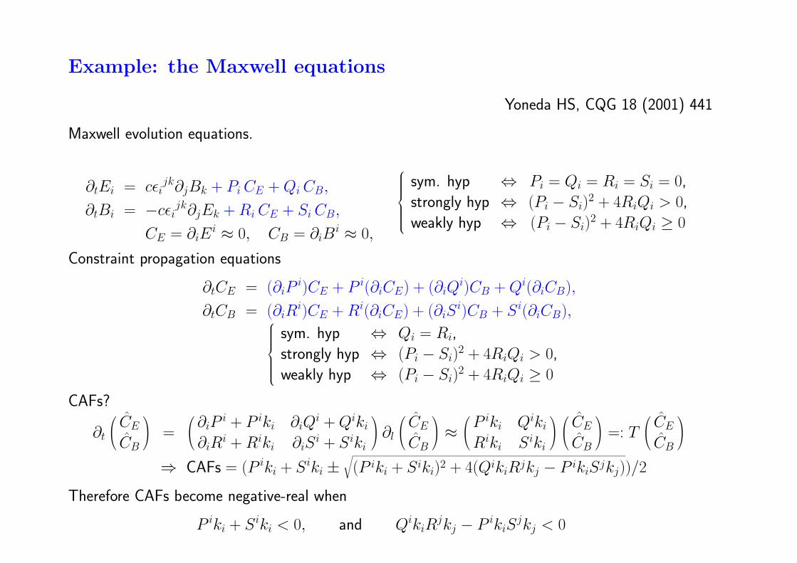
Example: the Maxwell equations
Yoneda HS, CQG 18 (2001) 441
Maxwell evolution equations.
!tEi = c"ijk!jBk + Pi CE + Qi CB,
!tBi = !c"ijk!jEk + Ri CE + Si CB,
CE = !iEi " 0, CB = !iB
i " 0,
!"""""#
"""""$
sym. hyp # Pi = Qi = Ri = Si = 0,strongly hyp # (Pi ! Si)2 + 4RiQi > 0,weakly hyp # (Pi ! Si)2 + 4RiQi $ 0
Constraint propagation equations
!tCE = (!iPi)CE + P i(!iCE) + (!iQ
i)CB + Qi(!iCB),
!tCB = (!iRi)CE + Ri(!iCE) + (!iS
i)CB + Si(!iCB),!"""""#
"""""$
sym. hyp # Qi = Ri,strongly hyp # (Pi ! Si)2 + 4RiQi > 0,weakly hyp # (Pi ! Si)2 + 4RiQi $ 0
CAFs?
!t
%
&CE
CB
'
( =%
&!iP i + P iki !iQi + Qiki
!iRi + Riki !iSi + Siki
'
( !l
%
&CE
CB
'
( "%
&P iki Qiki
Riki Siki
'
(
%
&CE
CB
'
( =: T%
&CE
CB
'
(
% CAFs = (P iki + Siki ±)(P iki + Siki)2 + 4(QikiRjkj ! P ikiSjkj))/2
Therefore CAFs become negative-real when
P iki + Siki < 0, and QikiRjkj ! P ikiS
jkj < 0

Adjusted-Maxwell system works as well.
INSTITUTE OF PHYSICS PUBLISHING CLASSICAL AND QUANTUM GRAVITY
Class. Quantum Grav. 18 (2001) 441–462 www.iop.org/Journals/cq PII: S0264-9381(01)15923-X
Hyperbolic formulations and numerical relativity: II.asymptotically constrained systems of Einsteinequations
Gen Yoneda1 and Hisa-aki Shinkai2
1 Department of Mathematical Sciences, Waseda University, Shinjuku, Tokyo, 169-8555, Japan2 Centre for Gravitational Physics and Geometry, 104 Davey Lab., Department of Physics, ThePennsylvania State University, University Park, PA 16802-6300, USA
E-mail: [email protected] and [email protected]
Received 27 July 2000, in final form 13 December 2000
AbstractWe study asymptotically constrained systems for numerical integration of theEinstein equations, which are intended to be robust against perturbative errorsfor the free evolution of the initial data. First, we examine the previouslyproposed ‘! system’, which introduces artificial flows to constraint surfacesbased on the symmetric hyperbolic formulation. We show that this systemworks as expected for the wave propagation problem in the Maxwell systemand in general relativity using Ashtekar’s connection formulation. Second, wepropose a new mechanism to control the stability, which we call the ‘adjustedsystem’. This is simply obtained by adding constraint terms in the dynamicalequations and adjusting their multipliers. We explain why a particular choiceof multiplier reduces the numerical errors from non-positive or pure-imaginaryeigenvalues of the adjusted constraint propagation equations. This ‘adjustedsystem’ is also tested in the Maxwell system and in the Ashtekar system. Thismechanism affects more than the system’s symmetric hyperbolicity.
PACS numbers: 0420C, 0425, 0425D
(Some figures in this article are in colour only in the electronic version; see www.iop.org)
1. Introduction
Numerical relativity, an approach to solving the Einstein equations numerically, is supposedto be the only way to study highly nonlinear gravitational phenomena. Although the attemptalready has decades of history, we still do not have a definite recipe for integrating the Einsteinequations that will give us accurate and long-term stable time evolutions. Here and hereafter,we mean by ‘stable evolution’ that the system keeps the violation of the constraints within asuitable small value in its free numerical evolution.
0264-9381/01/030441+22$30.00 © 2001 IOP Publishing Ltd Printed in the UK 441
454 G Yoneda and H Shinkai
a symmetric hyperbolic system (e.g. [2–5, 10]). We believe, however, that the above guidelinesyield the essential mechanism for our purpose of constructing a stable dynamical system.
In the following subsections and appendix A, we demonstrate that this adjusted systemactually works as desired in the Maxwell system and in the Ashtekar system of the Einsteinequations, in which the above two guidelines are applied, respectively.
3.2. Example 1: Maxwell equations
3.2.1. Adjusted system. Here we again consider the Maxwell equations (2.9)–(2.11). Westart from the adjusted dynamical equations
!tEi = c"ijk!jBk + PiCE + pj
i(!jCE) + QiCB + qji(!jCB), (3.7)
!tBi = !c"ijk!jEk + RiCE + rj
i(!jCE) + SiCB + sji(!jCB), (3.8)
where P, Q, R, S, p, q, r and s are multipliers. These dynamical equations adjust theconstraint propagation equations as
!tCE = (!iPi)CE + P i(!iCE) + (!iQ
i)CB + Qi(!iCB)
+(!ipji)(!jCE) + pji(!i!jCE) + (!iq
ji)(!jCB) + qji(!i!jCB), (3.9)
!tCB = (!iRi)CE + Ri(!iCE) + (!iS
i)CB + Si(!iCB)
+(!i rji)(!jCE) + rji(!i!jCE) + (!i s
ji)(!jCB) + sji(!i!jCB). (3.10)
This will be expressed using Fourier components by
!t
!
CE
CB
"
=!
!iPi + iP iki + ikj (!ip
ji) ! kikjpji !iQ
i + iQiki + ikj (!iqji) ! kikjq
ji
!iRi + iRiki + ikj (!i r
ji) ! kikj rji !iS
i + iSiki + ikj (!i sji) ! kikj s
ji
"
"!
CE
CB
"
=: T
!
CE
CB
"
. (3.11)
Assuming the multipliers are constants or functions of E and B, we can truncate the principalmatrix as
(0)T =!
iP iki ! kikjpji iQiki ! kikjq
ji
iRiki ! kikj rji iSiki ! kikj s
ji
"
, (3.12)
with eigenvalues
#± = p + s ±#
p2 + 4 q r ! 2 p s + s2
2, (3.13)
where p := iP iki ! kikjpji, q := iQiki ! kikjq
ji, r := iRiki ! kikj rji , s := iSiki ! kikj s
ji .
If we fix q = r = 0, then #± = p, s. Furthermore, if we assume pji, sji > 0, andset everything else to zero, then #± < 0, that is we can get all the eigenvalues which have anegative real part. That is, our guideline (a) is satisfied. (Conversely, if we choose q = r = 0and pji, sji < 0, then #± > 0.)
3.2.2. Numerical demonstration. We applied the above adjusted system to the same wavepropagation problem as in section 2.2.3. For simplicity, we fix $ = pij = sij and set othermultipliers equal to zero. In figure 4, we show the L2 norm of the constraint violation as afunction of time, with various $ . As was expected, we see better performance for $ > 0 (ofthe system with a negative real part of the constraint propagation equation), while divergingbehaviour for $ < 0 (of the system with a positive real part of the constraint propagationequation).
Hyperbolic formulations and numerical relativity: II 455
Figure 4. Demonstrations of the adjusted system in the Maxwell equation. We perform the sameexperiments with section 2.2.3 (figure 1). Constraint violation (L2 norm of CE ) versus time areplotted for various ! (= pj
i = sji ). We see that ! > 0 gives a better performance (i.e. negative
real part eigenvalues for the constraint propagation equation), while excessively large positive !makes the system divergent again.
3.3. Example 2: Einstein equations (Ashtekar equations)
3.3.1. Adjusted system for controlling constraint violations. Here we only consider theadjusted system which controls the departures from the constraint surface. In the appendix,we present an advanced system which controls the violation of the reality condition togetherwith a numerical demonstration.
Even if we restrict ourselves to adjusted equations of motion for (Eia, Aa
i ) with constraintterms (no adjustment with derivatives of constraints), generally, we could adjust them as
"t Eia = !iDj (#
cbaN" Ej
c Eib) + 2Dj (N
[j Ei]a ) + iAb
0#c
ab Eic + Xi
aCH + Y ija CMj + P ib
a CGb,
(3.14)
"tAai = !i#ab
cN" EjbF c
ij + NjF aji + DiAa
0 + $N"Ea
i + Qai CH + Ri
jaCMj + Zabi CGb, (3.15)
where Xia, Y
ija , Zab
i , P iba , Qa
i and Raji are multipliers. However, in order to simplify the
discussion, we restrict multipliers so as to reproduce the symmetric hyperbolic equationsof motion [10, 11], i.e.
X = Y = Z = 0,
P iba = !1(N
i%ba + iN
"#a
bcEic),
Qai = !2(e
!2N"Ea
i ),
Rija = !3(ie!2N
"#ac
bEbi E
jc ).
(3.16)
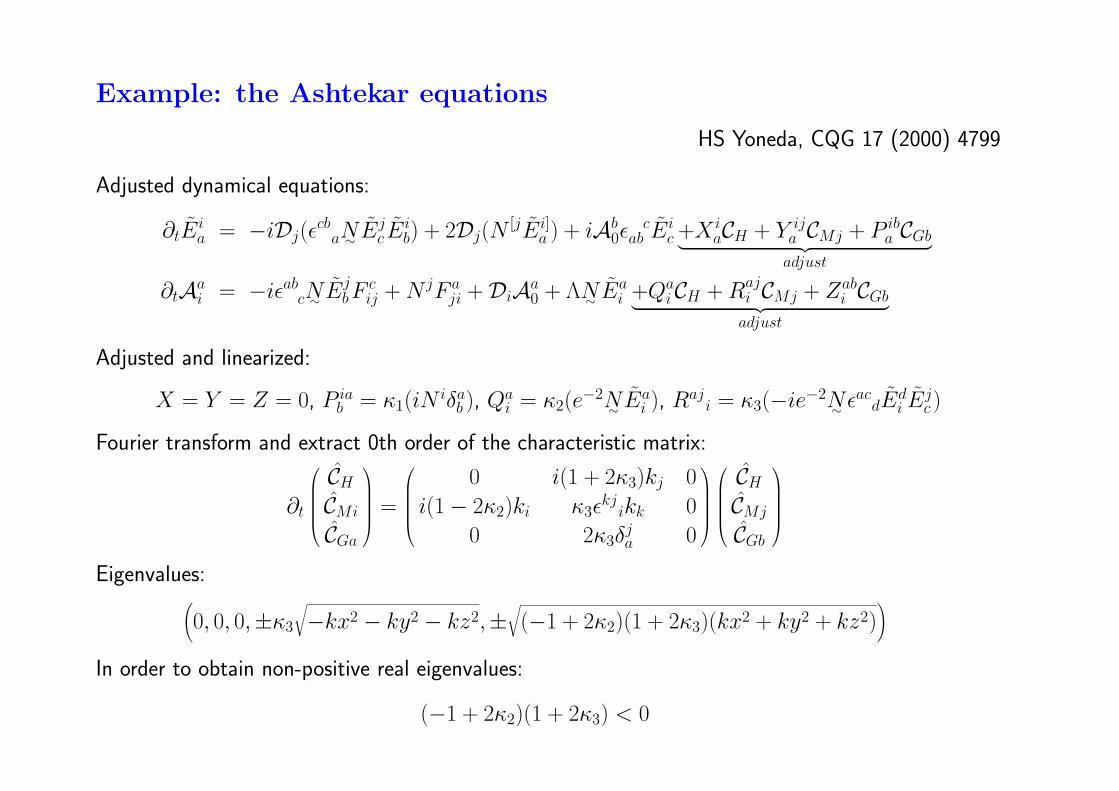
Example: the Ashtekar equations
HS Yoneda, CQG 17 (2000) 4799
Adjusted dynamical equations:
!tEia = !iDj("
cbaN" Ej
c Eib) + 2Dj(N
[jEi]a ) + iAb
0"c
ab Eic +Xi
aCH + Y ija CMj + P ib
a CGb! "# $adjust
!tAai = !i"ab
cN" EjbF
cij + NjFa
ji + DiAa0 + !N" Ea
i +QaiCH + Raj
i CMj + Zabi CGb! "# $
adjust
Adjusted and linearized:
X = Y = Z = 0, P iab = #1(iNi$a
b ), Qai = #2(e!2N" Ea
i ), Raji = #3(!ie!2N" "
acdEd
i Ejc )
Fourier transform and extract 0th order of the characteristic matrix:
!t
%
&&&&'
CH
CMi
CGa
(
))))*=
%
&&&&'
0 i(1 + 2#3)kj 0i(1 ! 2#2)ki #3"kj
ikk 00 2#3$j
a 0
(
))))*
%
&&&&'
CH
CMj
CGb
(
))))*
Eigenvalues:+
0, 0, 0,±#3
,
!kx2 ! ky2 ! kz2,±,
(!1 + 2#2)(1 + 2#3)(kx2 + ky2 + kz2)-
In order to obtain non-positive real eigenvalues:
(!1 + 2#2)(1 + 2#3) < 0

Adjusted-Ashtekar system works as well.
INSTITUTE OF PHYSICS PUBLISHING CLASSICAL AND QUANTUM GRAVITY
Class. Quantum Grav. 18 (2001) 441–462 www.iop.org/Journals/cq PII: S0264-9381(01)15923-X
Hyperbolic formulations and numerical relativity: II.asymptotically constrained systems of Einsteinequations
Gen Yoneda1 and Hisa-aki Shinkai2
1 Department of Mathematical Sciences, Waseda University, Shinjuku, Tokyo, 169-8555, Japan2 Centre for Gravitational Physics and Geometry, 104 Davey Lab., Department of Physics, ThePennsylvania State University, University Park, PA 16802-6300, USA
E-mail: [email protected] and [email protected]
Received 27 July 2000, in final form 13 December 2000
AbstractWe study asymptotically constrained systems for numerical integration of theEinstein equations, which are intended to be robust against perturbative errorsfor the free evolution of the initial data. First, we examine the previouslyproposed ‘! system’, which introduces artificial flows to constraint surfacesbased on the symmetric hyperbolic formulation. We show that this systemworks as expected for the wave propagation problem in the Maxwell systemand in general relativity using Ashtekar’s connection formulation. Second, wepropose a new mechanism to control the stability, which we call the ‘adjustedsystem’. This is simply obtained by adding constraint terms in the dynamicalequations and adjusting their multipliers. We explain why a particular choiceof multiplier reduces the numerical errors from non-positive or pure-imaginaryeigenvalues of the adjusted constraint propagation equations. This ‘adjustedsystem’ is also tested in the Maxwell system and in the Ashtekar system. Thismechanism affects more than the system’s symmetric hyperbolicity.
PACS numbers: 0420C, 0425, 0425D
(Some figures in this article are in colour only in the electronic version; see www.iop.org)
1. Introduction
Numerical relativity, an approach to solving the Einstein equations numerically, is supposedto be the only way to study highly nonlinear gravitational phenomena. Although the attemptalready has decades of history, we still do not have a definite recipe for integrating the Einsteinequations that will give us accurate and long-term stable time evolutions. Here and hereafter,we mean by ‘stable evolution’ that the system keeps the violation of the constraints within asuitable small value in its free numerical evolution.
0264-9381/01/030441+22$30.00 © 2001 IOP Publishing Ltd Printed in the UK 441
456 G Yoneda and H Shinkai
Figure 5. Demonstration of the adjusted system in the Ashtekar equation. We plot the violation ofthe constraint for the same model as figure 3(b). An artificial error term was added at t = 6, in theform of A2
y ! A2y(1 + error), where error is + 20% as before. (a), (b) L2 norm of the Hamiltonian
constraint equation, CH , and momentum constraint equation, CMx , respectively. The full curve isthe case of ! = 0, that is the case of ‘no adjusted’ original Ashtekar equation (weakly hyperbolicsystem). The dotted curve is for ! = 1, equivalent to the symmetric hyperbolic system. We seethat the other curve (! = 2.0) shows better performance than the symmetric hyperbolic case.
Hyperbolic formulations and numerical relativity: II 455
Figure 4. Demonstrations of the adjusted system in the Maxwell equation. We perform the sameexperiments with section 2.2.3 (figure 1). Constraint violation (L2 norm of CE ) versus time areplotted for various ! (= pj
i = sji ). We see that ! > 0 gives a better performance (i.e. negative
real part eigenvalues for the constraint propagation equation), while excessively large positive !makes the system divergent again.
3.3. Example 2: Einstein equations (Ashtekar equations)
3.3.1. Adjusted system for controlling constraint violations. Here we only consider theadjusted system which controls the departures from the constraint surface. In the appendix,we present an advanced system which controls the violation of the reality condition togetherwith a numerical demonstration.
Even if we restrict ourselves to adjusted equations of motion for (Eia, Aa
i ) with constraintterms (no adjustment with derivatives of constraints), generally, we could adjust them as
"t Eia = !iDj (#
cbaN" Ej
c Eib) + 2Dj (N
[j Ei]a ) + iAb
0#c
ab Eic + Xi
aCH + Y ija CMj + P ib
a CGb,
(3.14)
"tAai = !i#ab
cN" EjbF c
ij + NjF aji + DiAa
0 + $N"Ea
i + Qai CH + Ri
jaCMj + Zabi CGb, (3.15)
where Xia, Y
ija , Zab
i , P iba , Qa
i and Raji are multipliers. However, in order to simplify the
discussion, we restrict multipliers so as to reproduce the symmetric hyperbolic equationsof motion [10, 11], i.e.
X = Y = Z = 0,
P iba = !1(N
i%ba + iN
"#a
bcEic),
Qai = !2(e
!2N"Ea
i ),
Rija = !3(ie!2N
"#ac
bEbi E
jc ).
(3.16)

The Adjusted system (essentials):
Purpose: Control the violation of constraints by reformulating the system so as to have a
constrained surface an attractor.
Procedure: Add a particular combination of constraints to the evolution equations, and adjust
its multipliers.
Theoretical support: Eigenvalue analysis of the constraint propagation equations.
Advantages: Available even if the base system is not a symmetric hyperbolic.
Advantages: Keep the number of the variable same with the original system.
Conjecture on Constraint Amplification Factors (CAFs):
(A) If CAF has a negative real-part (the constraints are forced to be diminished), then we see more
stable evolution than a system which has positive CAF.
(B) If CAF has a non-zero imaginary-part (the constraints are propagating away), then we see more
stable evolution than a system which has zero CAF.

adjusted ADM (Shinkai-Yoneda)
87,95,99
Kidder-Scheel -Teukolsky
01
AEI
CaltechPennState
99
Shibata
2001
so-called BSSN
hyperbolic formulation
asymptotically constrained / constraint damping
adjusted-system01
Detweiler 02
adjusted BSSN (Yoneda-Shinkai)02
Nagy-Ortiz -Reula
04
04 Z4 (Bona et.al.)
Illinois
87
ADM62
BSSN
Bona-Masso92
lambda system Shinkai-Yoneda
harmonic92 Z4-lambda(Gundlach-Calabrese)
05

adjusted ADM (Shinkai-Yoneda)
87,95,99
Kidder-Scheel -Teukolsky
01
AEI
CaltechPennState
99
Shibata
LSU
2001 2005
so-called BSSN
hyperbolic formulation
asymptotically constrained / constraint damping
adjusted-system01
Detweiler 02
adjusted BSSN (Yoneda-Shinkai)02
Nagy-Ortiz -Reula
04
04 Z4 (Bona et.al.)
Illinois
Pretorius
87
ADM62
BSSN
Bona-Masso92
lambda system Shinkai-Yoneda
harmonic92 Z4-lambda(Gundlach-Calabrese)
05

adjusted ADM (Shinkai-Yoneda)
87,95,99
Kidder-Scheel -Teukolsky
01
AEI
CaltechPennState
99
Kiuchi-Shinkai
Shibata
LSU
2001 2005
so-called BSSN
hyperbolic formulation
asymptotically constrained / constraint damping
adjusted-system01
Detweiler 02
adjusted BSSN (Yoneda-Shinkai)02
Nagy-Ortiz -Reula
04
04 Z4 (Bona et.al.)
Illinois
NASA-Goddard
UTB-Rochester
Pretorius
87
ADM62
BSSN
Bona-Masso92
lambda system Shinkai-Yoneda
LSU Jena
harmonic92
PennState
Parma
Shinkai
BSSN is “well-posed” ?(Sarbach / Gundlach ...)
Z4-lambda(Gundlach-Calabrese)
05
Southampton
AEI