formulas and calculations for drilling operations second...
TRANSCRIPT

Formulas and Calculations
for Drilling Operations
Second Edition

Scrivener Publishing
100 Cummings Center, Suite 541J
Beverly, MA 01915-6106
Publishers at Scrivener
Martin Scrivener ([email protected])
Phillip Carmical ([email protected])

Formulas and Calculations
for Drilling Operations
Second Edition
James G. Speight

This edition first published 2018 by John Wiley & Sons, Inc., 111 River Street, Hoboken, NJ 07030, USA
and Scrivener Publishing LLC, 100 Cummings Center, Suite 541J, Beverly, MA 01915, USA
© 2018 Scrivener Publishing LLC
For more information about Scrivener publications please visit www.scrivenerpublishing.com.
All rights reserved. No part of this publication may be reproduced, stored in a retrieval system, or
transmitted, in any form or by any means, electronic, mechanical, photocopying, recording, or other-
wise, except as permitted by law. Advice on how to obtain permission to reuse material from this title
is available at http://www.wiley.com/go/permissions.
Wiley Global Headquarters
111 River Street, Hoboken, NJ 07030, USA
For details of our global editorial offices, customer services, and more information about Wiley prod-
ucts visit us at www.wiley.com.
Limit of Liability/Disclaimer of Warranty
While the publisher and authors have used their best efforts in preparing this work, they make no rep-
resentations or warranties with respect to the accuracy or completeness of the contents of this work and
specifically disclaim all warranties, including without limitation any implied warranties of merchant-
ability or fitness for a particular purpose. No warranty may be created or extended by sales representa-
tives, written sales materials, or promotional statements for this work. The fact that an organization,
website, or product is referred to in this work as a citation and/or potential source of further informa-
tion does not mean that the publisher and authors endorse the information or services the organiza-
tion, website, or product may provide or recommendations it may make. This work is sold with the
understanding that the publisher is not engaged in rendering professional services. The advice and
strategies contained herein may not be suitable for your situation. You should consult with a specialist
where appropriate. Neither the publisher nor authors shall be liable for any loss of profit or any other
commercial damages, including but not limited to special, incidental, consequential, or other damages.
Further, readers should be aware that websites listed in this work may have changed or disappeared
between when this work was written and when it is read.
Library of Congress Cataloging-in-Publication DataISBN 978-1-119-08362-7
Cover design by Kris Hackerott
Set in size of 11pt and Minion Pro by Exeter Premedia Services Private Ltd., Chennai, India
Printed in the USA
10 9 8 7 6 5 4 3 2 1

v
Contents
Preface xiii
1 Standard Formulas and Calculations 11.01 Abrasion Index 11.02 Acid Number 31.03 Acidity and Alkalinity 31.04 Annular Velocity 41.05 Antoine Equation 51.06 API Gravity Kilograms per Liter/Pounds per Gallon 51.07 Barrel Conversion to other Units. 151.08 Bernoulli’s Principle 151.09 Brine 161.10 Bubble Point and Bubble Point Pressure 161.11 Buoyancy, Buoyed Weight, and Buoyancy Factor 181.12 Capacity 19
1.12.1 Hole (Pipe, Tubing) Capacity (in barrels per one linear foot, bbl/ft) 20
1.12.2 Annular Capacity 201.12.3 Annular Volume
(volume between casing and tubing, bbl) 201.13 Capillary Number 211.14 Capillary Pressure 211.15 Cementation Value 221.16 Composite Materials 231.17 Compressibility 231.18 Darcy’s Law 251.19 Dew Point Temperature and Pressure 261.20 Displacement 271.21 Effective Weight 281.22 Flow Through Permeable Media 29
1.22.1 Productivity Index 291.22.2 Steady-State Flow 29

vi Contents
1.22.3 Linear Flow 391.22.4 Spherical Flow 39
1.23 Flow Through Porous Media 391.24 Flow Velocity 401.25 Fluid Saturation 411.26 Formation Volume Factor Gas 411.27 Formation Volume Factor Oil 421.28 Friction 42
1.28.1 Coefficient of Friction 421.28.2 Types of Friction 431.28.3 Friction and Rotational Speed 43
1.29 Gas Deviation Factor 431.30 Gas Solubility 441.31 Gas-Oil Ratio 441.32 Geothermal Gradient 451.33 Hole Capacity 451.34 Horsepower 501.35 Hydrostatic Pressure 511.36 Isothermal Compressibility of Oil 511.37 Marx-Langenheim Model 521.38 Material Balance 531.39 Modulus of Elasticity 551.40 Oil and Gas Originally in Place 551.41 Oil Recovery Factor 561.42 Permeability 571.43 Poisson’s Ratio 571.44 Porosity 591.45 Pressure Differentials 611.46 Productivity Index 621.47 PVT Properties 62
1.47.1 Specific Gravity and Molecular Weight 621.47.2 Isothermal Compressibility 621.47.3 Undersaturated Oil Formation Volume Factor 631.47.4 Oil Density 631.47.5 Dead Oil Viscosity 631.47.6 Undersaturated Oil Viscosity 631.47.7 Gas/Oil Interfacial Tension 631.47.8 Water/Oil Interfacial Tension 63
1.48 Reserves Estimation 651.49 Reservoir Pressure 651.50 Resource Estimation 67

Contents vii
1.51 Reynold’s Number 671.52 Saturated Steam 671.53 Standard Oilfield Measurements 681.54 Twist 691.55 Ultimate Tensile Strength 701.56 Volume Flow Rate 701.57 Volumetric Factors 711.58 Yield Point 72
2 RIG Equipment 732.01 API Casing Grades 732.02 Block Efficiency Factor 742.03 Blocks and Drilling Line 742.04 Crown Block Capacity 752.05 Derrick Load 762.06 Energy Transfer 772.07 Engine Efficiency 782.08 Line Pull Efficiency Factor 792.09 Mud Pump 79
2.09.1 Volume of Fluid Displaced 802.09.2 Volumetric Efficiency 802.09.3 Pump Factor 81
2.10 Offshore Vessels 812.10.1 Terminology 822.10.2 Environmental Forces 832.10.3 Riser Angle 83
2.11 Rotary Power 852.12 Ton-Miles Calculations 85
2.12.1 Round-Trip Ton Miles Calculations 862.12.2 Drilling Ton-Miles Calculations 862.12.3 Coring Ton-Miles Calculations 862.12.4 Casing Ton-Miles Calculations 86
3 Well Path Design 893.01 Average Curvature-Average Dogleg Severity 893.02 Bending Angle 893.03 Borehole Curvature 90
3.03.1 General Formula 903.03.2 Borehole Radius of Curvature 90
3.04 Borehole Torsion 913.04.1 General Method 913.04.2 Cylindrical Helical Method 91

viii Contents
3.05 Horizontal Displacement 923.06 Magnetic Reference and Interference 933.07 Tool Face Angle 943.08 Tool Face Angle Change 963.09 Tortuosity 97
3.09.1 Absolute and Relative Tortuosity 973.09.2 Sine Wave Method 983.09.3 Helical Method 993.09.4 Random Inclination Azimuth Method 993.09.5 Random Inclination Dependent Azimuth Method 100
3.10 Types of Wellpath Designs 1003.11 Vertical and Horizontal Curvatures 1003.12 Wellbore Trajectory Uncertainty 1013.13 Wellpath Length Calculations 103
4 Fluids 1054.01 Acidity-Alkalinity 1054.02 Base Fluid – Water-Oil Ratios 1064.03 Common Weighting Materials 1074.04 Diluting Mud 1084.05 Drilling Fluid Composition 1094.06 Equivalent Mud Weight 1104.07 Fluid Loss 1104.08 Marsh Funnel 1124.09 Mud Rheology 1124.10 Mud Weighting 1144.11 Plastic Viscosity, Yield Point, and Zero-Sec Gel 116
4.11.1 Bingham, Plastic Model 1164.11.2 Shear Stress and Shear Rate 1174.11.3 Power Law 117
4.12 Reynolds Number and Critical Velocity 1184.13 Slip Velocity 118
5 Hydraulics 1215.01 Basic Calculations 121
5.01.1 Critical Velocity 1215.01.2 Pump Calculations 121
5.02 Bingham Plastic Model 1225.03 Bit Hydraulics 124
5.03.1 Common Calculations 1245.03.2 Optimization Calculations 125

Contents ix
5.03.2.1 Limitation 1 – Available Pump Horsepower 1265.03.2.2 Limitation 2 – Surface Operating Pressure 126
5.04 Critical Transport Fluid Velocity 1275.05 Equivalent Circulating Density 1275.06 Equivalent Mud Weight 1275.07 Gel Breaking Pressure 1285.08 Hole Cleaning – Cuttings Transport 128
6 Tubular Mechanics 1316.01 API Casing and Liners – Weight, Dimensions, Capacity,
and Displacement 1316.02 API Drill Pipe Capacity and Displacement 1346.03 Bending Stress Ratio 1356.04 Buckling Force 1356.05 Drag Force 1366.06 Drill Collar Length 1376.07 Fatigue Ratio 1386.08 Length Change Calculations 1386.09 Maximum Permissible Dogleg 1396.10 Pipe Wall Thickness and other Dimensions 1406.11 Slip Crushing 1406.12 Stress 145
6.12.1 Radial Stress 1456.12.2 Tangential Stress 1456.12.3 Longitudinal Stress 1456.12.4 Stress Ratio 146
6.13 Tension 1466.14 Torque 146
7 Drilling Tools 1497.01 Backoff Calculations 1497.02 Downhole Turbine 1527.03 Jar Calculations 153
7.03.1 Force Calculations for Up Jars 1537.03.2 Force Calculations for Down Jars 153
7.04 Overpull/Slack-off Calculations 1557.05 Percussion Hammer 1577.06 Positive Displacement Motor (PDM) 1577.07 Rotor Nozzle Sizing 1577.08 Stretch Calculations 159

x Contents
8 Pore Pressure and Fracture Gradient 1618.01 Formation Pressure 161
8.01.1 Hubert and Willis Correlation 1618.01.2 Matthews and Kelly Correlation 1628.01.3 Eaton’s Correlation 1638.01.4 Christman’s Correlation 163
8.02 Leak-off Pressure 163
9 Well Control 1659.01 Accumulators 1659.02 Driller’s Method 1669.03 Formulas Used in Kick and Kill Procedures 1679.04 Hydrostatic Pressure Due to the Gas Column 1689.05 Kill Methods 1689.06 Kill Mud Weight 1699.07 Leak-off Pressure 1709.08 Length and Density of the Kick 171
9.08.1 Length of the Kick 1719.08.2 Density of the Kick 1719.08.3 Type of Kick 1729.08.4 Kick Classification 1729.08.5 Kick Tolerance 173
9.09 Maximum Allowable Annular Surface Pressure 1749.10 Riser Margin 175
10 Drilling Problems 17710.01 Differential Sticking Force 177
10.01.1 Method 1 17810.01.2 Method 2 17810.01.3 Method 3 179
10.02 Hole Cleaning – Slip Velocity Calculations 17910.02.1 Chien Correlation 17910.02.2 Moore Correlation 18010.02.3 Walker-Mays Correlation 180
10.03 Increased Equivalent Circulating Density (ECD) Due to Cuttings 181
10.04 Keyseating 18210.05 Lost Circulation 18310.06 Common Minerals and Metals Encountered During
Drilling Operations 18510.07 Mud Weight Increase Due to Cuttings 18510.08 Pressure Loss in the Drill String 18610.09 Spotting Fluid Requirements 187
Contents xi
11 Cementing 18911.01 API Classification of Cement 18911.02 Cement: Physical Properties of Additives 19111.03 Cement Plug 19211.04 Cement Slurry Requirements 19411.05 Contact Time 19511.06 Gas Migration Potential 19511.07 Hydrostatic Pressure Reduction 19611.08 Portland Cement – Typical Components 19711.09 Slurry Density 19811.10 Yield of Cement 198
12 Well Cost 19912.01 Drilling Cost 19912.02 Expected Value 20012.03 Future Value 20012.04 Price Elasticity 201
13 Appendices 203
Glossary 243
Bibliography and Information Sources 273
About the Author 277
Index 279

xiii
Preface
Drilling engineers design and implement procedures to drill wells as safely and economically as possible. Drilling engineers are often degreed as petroleum engineers, although they may come from other technical disci-plines (such as mechanical engineering, geology, or chemical engineering) and subsequently be trained by an oil and gas company. The drilling engi-neering also may have practical experience as a rig hand or mud-logger or mud engineer.
The drilling engineer, whatever his/her educational background, must work closely with the drilling contractor, service contractors, and compli-ance personnel, as well as with geologists, chemists, and other technical specialists. The drilling engineer has the responsibility for ensuring that costs are minimized while getting information to evaluate the formations penetrated, protecting the health and safety of workers and other person-nel, and protecting the environment. Furthermore, to accomplish the task associated with well drilling and crude oil (or natural gas production) it is essential that the drilling engineers has a convenient source of references to definitions, formulas and examples of calculations.
This Second Edition continues as an introductory test for drilling engi-neers, students, lecturers, teachers, software programmers, testers, and researchers. The intent is to provide basic equations and formulas with the calculations for downhole drilling. In addition, where helpful, example calculations are included to show how the formula can be employed to provide meaningful data for the drilling engineer.
The book will provide a guide to exploring and explaining the various aspects of drilling engineering and will continue to serve as a tutorial guide for students, lecturers, and teachers as a solution manual and is a source for solving problems for drilling engineers.
For those users who require more details of the various terms and/or explanation of the terminology, the book also contain a comprehensive

xiv Preface
bibliography and a Glossary for those readers/users who require an expla-nation of the various terms. There is also an Appendix that contains valu-able data in a variety of tabular forms that the user will find useful when converting the various units used by the drilling engineer.
Dr. James Speight,Laramie, Wyoming.
January 2018.

1
1Standard Formulas and Calculations
1.01 Abrasion Index
The abrasion index (sometimes referred to as the wear index) is a measure of equipment (such as drill bit) wear and deterioration. At first approxima-tion, the wear is proportional to the rate of fuel flow in the third power and the maximum intensity of wear in millimeters) can be expressed:
δpl α η k m ω3 τ
δpl maximum intensity of plate wear, mm.α abrasion index, mm s3/g h.η coefficient, determining the number of probable attacks on the plate surface.k concentration of fuel in flow, g/m3.m coefficient of wear resistance of metal;w velocity of fuel flow, meters/sec.τ operation time, hours.
Formulas and Calculations for Drilling Operations, Second Edition.James G. Speight.
© 2018 Scrivener Publishing LLC. Published 2018 by John Wiley & Sons, Inc.

2 Formulas and Calculations for Drilling Operations
The resistance of materials and structures to abrasion can be measured by a variety of test methods (Table 1.1) which often use a specified abrasive or other controlled means of abrasion. Under the conditions of the test, the results can be reported or can be compared items subjected to similar tests. Theses standardized measurements can be employed to produce two sets of data: (1) the abrasion rate, which is the amount of mass lost per
Table 1.1 Examples of Selected ASTM Standard Test Method for Determining
Abrasion*.
ASTM B611 Test Method for Abrasive Wear Resistance of Cemented
Carbides
ASTM C131 Standard Test Method for Resistance to Degradation of
Small-Size Coarse Aggregate by Abrasion and Impact in the
Los Angeles Machine
ASTM C535 Standard Test Method for Resistance to Degradation of
Large-Size Coarse Aggregate by Abrasion and Impact in the
Los Angeles Machine
ASTM C944 Standard Test Method for Abrasion Resistance of Concrete
or Mortar Surfaces by the Rotating-Cutter Method
ASTM C1353 Standard Test Method for Abrasion Resistance of Dimension
Stone Subjected to Foot Traffic Using a Rotary Platform,
Double-Head Abraser
ASTM D 2228 Standard Test Method for Rubber Property Relative
Abrasion Resistance by the Pico Abrader Method
ASTM D4158 Standard Guide for Abrasion Resistance of Textile Fabrics,
see Martindale method
ASTM D7428 Standard Test Method for Resistance of Fine Aggregate to
Degradation by Abrasion in the Micro-Deval Apparatus
ASTM G81 Standard Test Method for Jaw Crusher Gouging Abrasion
Test
ASTM G105 Standard Test Method for Conducting Wet Sand/Rubber
Wheel Abrasion Tests
ASTM G132 Standard Test Method for Pin Abrasion Testing
ASTM G171 Standard Test Method for Scratch Hardness of Materials
Using a Diamond Stylus
ASTM G174 Standard Test Method for Measuring Abrasion Resistance of
Materials by Abrasive Loop Contact
*ASTM International, West Conshohocken, Pennsylvania; test methods are also available
from other standards organizations.

Standard Formulas and Calculations 3
1000 cycles of abrasion, and (2) the normalized abrasion rate, which is also called the abrasion resistance index and which is the ratio of the abrasion rate (i.e., mass lost per 1000 cycles of abrasion) with the known abrasion rate for some specific reference material.
1.02 Acid Number
The acid number (acid value, neutralization number, acidity) is the mass of potassium hydroxide (KOH) in milligrams that is required to neutralize one gram of the substance (ASTM D664, ASTM D974).
AN (Veq
beq
)N(56.1/Woil
)
Veq
is the amount of titrant (ml) consumed by the crude oil sample and 1 ml spiking solution at the equivalent point, b
eq is the amount of titrant
(ml) consumed by 1 ml spiking solution at the equivalent point, and 56.1 is the molecular weight of potassium hydroxide.
1.03 Acidity and Alkalinity
pH is given as the negative logarithm of [H+] or [OH ] and is a mea-surement of the acidity of a solution and can be compared by using the following:
pH log([H+]
pH log([OH ]
[H+] or [OH ] are hydrogen and hydroxide ion concentrations, respec-tively, in moles/litter. Also, at room temperature, pH pOH 14. For other temperatures:
pH pOH pKw
Kw is the ion product constant at that particular temperature. At room
temperature, the ion product constant for water is 1.0 10 14 moles/litter (mol/L or M). A solution in which [H+=] [OH ] is acidic, and a solution in which [H+=] [OH ] is basic (Table 1.2).

4 Formulas and Calculations for Drilling Operations
1.04 Annular Velocity
Three main factors affecting annular velocity are size of hole (bigger ID), size of drill pipe (smaller OD) and pump rate. Thus:
Annular velocity, ft/min = Flow rate, bbl/min ÷ annular capacity, bbl/ft
For example, with a flow rate of 10 bbl/min and an annular capacity of 0.13 bbl/ft, the annular velocity is:
10 bbl/min 0.13 bbl/ft which is 76.92 ft/min.
Other formulas include:
Annular velocity, ft/min = (24.5 × Q) ÷ (Dh2 Dp2)
where Q is the flow rate in gpm, Dh is inside diameter of casing or hole size in inches, and Dp is outside diameter of pipe, tubing or collars in inch. Thus, for a flow rate of 800 gpm, a hole size of 10 inches, a drill pipe OD of 5 inches, the annular velocity is
Annular velocity (24.5 800) (102 52) 261 ft/min
Another formula used is:
Annular Velocity, ft/min = Flow rate (Q), bbl/min × 1029.4 ÷ (Dh2 Dp2).
Thus, for a flow rate equal to 13 bbl/min, a hole size of 10 inches, and a drill pipe OD of 5 inches, the annular velocity is:
13 bbl/min 1029.4 (102 52) 178.43 ft/min
Table 1.2 Ranges of Acidity and Alkalinity.
pH [H+] Property
<7 >1.0 10 7 M Acid
7 1.0 10 7 M Neutral
>7 <1.0 10 7 M Basic
Standard Formulas and Calculations 5
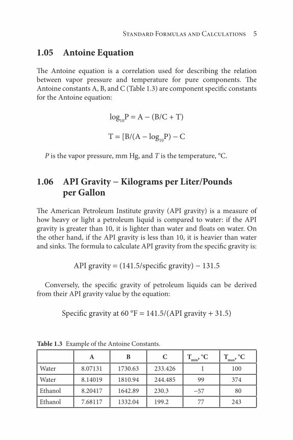
1.05 Antoine Equation
The Antoine equation is a correlation used for describing the relation between vapor pressure and temperature for pure components. The Antoine constants A, B, and C (Table 1.3) are component specific constants for the Antoine equation:
log10
P A (B/C + T)
T [B/(A log10
P) C
P is the vapor pressure, mm Hg, and T is the temperature, °C.
1.06 API Gravity Kilograms per Liter/Pounds per Gallon
The American Petroleum Institute gravity (API gravity) is a measure of how heavy or light a petroleum liquid is compared to water: if the API gravity is greater than 10, it is lighter than water and floats on water. On the other hand, if the API gravity is less than 10, it is heavier than water and sinks. The formula to calculate API gravity from the specific gravity is:
API gravity (141.5/specific gravity) 131.5
Conversely, the specific gravity of petroleum liquids can be derived from their API gravity value by the equation:
Specific gravity at 60 °F 141.5/(API gravity 31.5)
Table 1.3 Example of the Antoine Constants.
A B C Tmin
, °C Tmax
, °C
Water 8.07131 1730.63 233.426 1 100
Water 8.14019 1810.94 244.485 99 374
Ethanol 8.20417 1642.89 230.3 57 80
Ethanol 7.68117 1332.04 199.2 77 243

6 Formulas and Calculations for Drilling Operations
Using the API gravity, it is possible to calculate the approximate number of of crude oil per metric ton. Thus:
Barrels of crude oil per metric ton(API gravity 131.5)/(141.5 0.159)
The relationship between the API gravity of crude oil and kilograms per liter or pounds per gallon is presented in the table (Table 1.4) below.
Table 1.4 API Gravity Conversion to Kilograms per Liter/Pounds per Gallon
API gravity Specific gravity
Kilograms per
liter
Pounds per
gallon
1 1.0679 1.0658 8.8964
1.5 1.0639 1.0618 8.863
2 1.0599 1.0578 8.8298
2.5 1.056 1.0539 8.7968
3 1.052 1.0499 8.7641
3.5 1.0481 1.0461 8.7317
4 1.0443 1.0422 8.6994
4.5 1.0404 1.0384 8.6674
5 1.0366 1.0346 8.6357
5.5 1.0328 1.0308 8.6042
6 1.0291 1.027 8.5729
6.5 1.0254 1.0233 8.5418
7 1.0217 1.0196 8.511
7.5 1.018 1.0159 8.4804
8 1.0143 1.0123 8.45
8.5 1.0107 1.0087 8.4198
9 1.0071 1.0051 8.3898
9.5 1.0035 1.0015 8.3601
10 1 0.998 8.3306
10.5 0.9965 0.9945 8.3012
11 0.993 0.991 8.2721
11.5 0.9895 0.9875 8.2432
(Continued)

Standard Formulas and Calculations 7
Table 1.4 Cont.
API gravity Specific gravity
Kilograms per
liter
Pounds per
gallon
12 0.9861 0.9841 8.2144
12.5 0.9826 0.9807 8.1859
13 0.9792 0.9773 8.1576
13.5 0.9759 0.9739 8.1295
14 0.9725 0.9706 8.1015
14.5 0.9692 0.9672 8.0738
15 0.9659 0.9639 8.0462
15.5 0.9626 0.9607 8.0189
16 0.9593 0.9574 7.9917
16.5 0.9561 0.9542 7.9647
17 0.9529 0.951 7.9379
17.5 0.9497 0.9478 7.9112
18 0.9465 0.9446 7.8848
18.5 0.9433 0.9414 7.8585
19 0.9402 0.9383 7.8324
19.5 0.9371 0.9352 7.8064
20 0.934 0.9321 7.7807
20.5 0.9309 0.9291 7.7551
21 0.9279 0.926 7.7297
21.5 0.9248 0.923 7.7044
22 0.9218 0.92 7.6793
22.5 0.9188 0.917 7.6544
23 0.9159 0.914 7.6296
23.5 0.9129 0.9111 7.605
24 0.91 0.9081 7.5805
24.5 0.9071 0.9052 7.5562
25 0.9042 0.9023 7.5321
25.5 0.9013 0.8995 7.5081
26 0.8984 0.8966 7.4843
26.5 0.8956 0.8938 7.4606
(Continued)

8 Formulas and Calculations for Drilling Operations
Table 1.4 Cont.
API gravity Specific gravity
Kilograms per
liter
Pounds per
gallon
27 0.8927 0.891 7.4371
27.5 0.8899 0.8882 7.4137
28 0.8871 0.8854 7.3904
28.5 0.8844 0.8826 7.3673
29 0.8816 0.8799 7.3444
29.5 0.8789 0.8771 7.3216
30 0.8762 0.8744 7.2989
30.5 0.8735 0.8717 7.2764
31 0.8708 0.869 7.254
31.5 0.8681 0.8664 7.2317
32 0.8654 0.8637 7.2096
32.5 0.8628 0.8611 7.1876
33 0.8602 0.8585 7.1658
33.5 0.8576 0.8559 7.1441
34 0.855 0.8533 7.1225
34.5 0.8524 0.8507 7.101
35 0.8498 0.8482 7.0797
35.5 0.8473 0.8456 7.0585
36 0.8448 0.8431 7.0375
36.5 0.8423 0.8406 7.0165
37 0.8398 0.8381 6.9957
37.5 0.8373 0.8356 6.975
38 0.8348 0.8331 6.9544
38.5 0.8324 0.8307 6.934
39 0.8299 0.8283 6.9136
39.5 0.8275 0.8258 6.8934
40 0.8251 0.8234 6.8733
40.5 0.8227 0.821 6.8533
41 0.8203 0.8186 6.8335
41.5 0.8179 0.8163 6.8137
(Continued)

Standard Formulas and Calculations 9
Table 1.4 Cont.
API gravity Specific gravity
Kilograms per
liter
Pounds per
gallon
42 0.8156 0.8139 6.7941
42.5 0.8132 0.8116 6.7746
43 0.8109 0.8093 6.7551
43.5 0.8086 0.807 6.7358
44 0.8063 0.8047 6.7167
44.5 0.804 0.8024 6.6976
45 0.8017 0.8001 6.6786
45.5 0.7994 0.7978 6.6597
46 0.7972 0.7956 6.641
46.5 0.7949 0.7934 6.6223
47 0.7927 0.7911 6.6038
47.5 0.7905 0.7889 6.5853
48 0.7883 0.7867 6.567
48.5 0.7861 0.7845 6.5487
49 0.7839 0.7824 6.5306
49.5 0.7818 0.7802 6.5126
50 0.7796 0.7781 6.4946
50.5 0.7775 0.7759 6.4768
51 0.7753 0.7738 6.459
51.5 0.7732 0.7717 6.4414
52 0.7711 0.7696 6.4238
52.5 0.769 0.7675 6.4064
53 0.7669 0.7654 6.389
53.5 0.7649 0.7633 6.3717
54 0.7628 0.7613 6.3546
54.5 0.7608 0.7592 6.3375
55 0.7587 0.7572 6.3205
55.5 0.7567 0.7552 6.3036
56 0.7547 0.7532 6.2868
56.5 0.7527 0.7512 6.2701
(Continued)

10 Formulas and Calculations for Drilling Operations
Table 1.4 Cont.
API gravity Specific gravity
Kilograms per
liter
Pounds per
gallon
57 0.7507 0.7492 6.2534
57.5 0.7487 0.7472 6.2369
58 0.7467 0.7452 6.2204
58.5 0.7447 0.7432 6.2041
59 0.7428 0.7413 6.1878
59.5 0.7408 0.7394 6.1716
60 0.7389 0.7374 6.1555
60.5 0.737 0.7355 6.1394
61 0.7351 0.7336 6.1235
61.5 0.7332 0.7317 6.1076
62 0.7313 0.7298 6.0918
62.5 0.7294 0.7279 6.0761
63 0.7275 0.7261 6.0605
63.5 0.7256 0.7242 6.045
64 0.7238 0.7223 6.0295
64.5 0.7219 0.7205 6.0141
65 0.7201 0.7187 5.9988
65.5 0.7183 0.7168 5.9836
66 0.7165 0.715 5.9685
66.5 0.7146 0.7132 5.9534
67 0.7128 0.7114 5.9384
67.5 0.7111 0.7096 5.9235
68 0.7093 0.7079 5.9086
68.5 0.7075 0.7061 5.8939
69 0.7057 0.7043 5.8792
69.5 0.704 0.7026 5.8645
70 0.7022 0.7008 5.85
70.5 0.7005 0.6991 5.8355
71 0.6988 0.6974 5.8211
71.5 0.697 0.6957 5.8068
(Continued)

Standard Formulas and Calculations 11
Table 1.4 Cont.
API gravity Specific gravity
Kilograms per
liter
Pounds per
gallon
72 0.6953 0.6939 5.7925
72.5 0.6936 0.6922 5.7783
73 0.6919 0.6905 5.7642
73.5 0.6902 0.6889 5.7501
74 0.6886 0.6872 5.7361
74.5 0.6869 0.6855 5.7222
75 0.6852 0.6839 5.7083
Table 1.5 API Gravity and Sulfur Content of Selected Heavy Oils.
API Sulfur % w/w
Bachaquero 13.0 2.6
Boscan 10.1 5.5
Cold Lake 13.2 4.1
Huntington Beach 19.4 2.0
Kern River 13.3 1.1
Lagunillas 17.0 2.2
Lloydminster 16.0 2.6
Lost Hills 18.4 1.0
Merey 18.0 2.3
Midway Sunset 12.6 1.6
Monterey 12.2 2.3
Morichal 11.7 2.7
Mount Poso 16.0 0.7
Pilon 13.8 1.9
San Ardo 12.2 2.3
Tremblador 19.0 0.8
Tia Juana 12.1 2.7
Wilmington 17.1 1.7
Zuata Sweet 15.7 2.7

12 Formulas and Calculations for Drilling OperationsT
able
1.6
A
PI
Gra
vity
at
Ob
serv
ed T
emp
erat
ure
Ver
sus
AP
I G
ravi
ty a
t 6
0 °
F
Ob
serv
ed
tem
per
atu
re (
°F)
18
.01
9.0
20
.02
1.0
22
.02
3.0
24
.02
5.0
26
.02
7.0
70
17
.5I8
.41
9.4
20
.42
1.4
22
.42
3.4
24
.42
5.4
26
.3
75
17
.2I8
.21
9.1
20
.12
1.1
22
.12
3.1
24
.12
5.0
26
.0
80
16
.91
7.9
ia.9
19
.a2
0.a
21
.a2
2.S
23
.72
4.7
25
.7
85
16
.61
7.6
ia.6
19
.62
0.5
21
.52
2.5
23
.42
4.4
25
.4
90
16
.41
7.3
is.3
19
.32
0.2
21
.22
2.2
23
.12
4.1
25
.1
95
16
.11
7.1
13
.01
9.0
20
.02
0.9
21
.92
2.S
23
.S2
4.S
10
01
5.9
16
.a1
7.8
18
.71
9.7
20
.62
1.6
22
.52
3.5
24
.4
10
51
5.6
16
.51
7.5
18
.71
9.4
20
.32
1.3
22
.22
3.2
24
.1
11
01
5.3
16
.31
7.2
18
.21
9.1
20
.12
1.0
21
.92
2.9
23
.B
11
51
5.1
16
.01
7.0
17
.9la
.a1
9.a
20
.72
1.6
22
.62
3.5
12
01
4.8
15
.8a
16
.71
7.6
ia.6
19
.52
0.4
21
.32
2.3
23
.2
12
51
4.6
15
.51
6.4
17
.4ia
.31
9.2
20
.12
1.1
22
.02
2.9
13
01
4.3
15
.21
6.2
17
.4la
.oIS
.91
9.9
20
.S2
1.7
22
.6
13
51
4.1
15
.01
5.9
16
.B1
7.7
IS.7
19
.62
0.5
21
.42
2.6
14
01
3.S
14
.71
5.6
16
.61
7.5
IS.4
19
.32
0.2
21
.12
2.0

Standard Formulas and Calculations 13
Table 1.7 Selected Crude Oils Showing the Differences in API Gravity and
Sulfur Content Within a Country.
Country Crude oil API
Sulfur %
w/w
Abu Dhabi (UAE) Abu Al Bu Khoosh 31.6 2.00
Abu Dhabi (UAE) Murban 40.5 0.78
Angola Cabinda 31.7 0.17
Angola Palanca 40.1 0.11
Australia Barrow Island 37.3 0.05
Australia Griffin 55.0 0.03
Brazil Garoupa 30.0 0.68
Brazil Sergipano Platforma 38.4 0.19
Brunei Champion Export 23.9 0.12
Brunei Seria 40.5 0.06
Cameroon Lokele 20.7 0.46
Cameroon Kole Marine 32.6 0.33
Canada (Alberta) Wainwright-Kinsella 23.1 2.58
Canada (Alberta) Rainbow 40.7 0.50
China Shengli 24.2 1.00
China Nanhai Light 40.6 0.06
Dubai (UAE) Fateh 31.1 2.00
Dubai (UAE) Margham Light 50.3 0.04
Egypt Ras Gharib 21.5 3.64
Egypt Gulf of Suez 31.9 1.52
Gabon Gamba 31.4 0.09
Gabon Rabi-Kounga 33.5 0.07
Indonesia Bima 21.1 0.25
Indonesia Kakap 51.5 0.05
Iran Aboozar (Ardeshir) 26.9 2.48
Iran Rostam 35.9 1.55
Iraq Basrah Heavy 24.7 3.50
Iraq Basrah Light 33.7 1.95
Libya Buri 26.2 1.76
Libya Bu Attifel 43.3 0.04
(Continued)

14 Formulas and Calculations for Drilling Operations
Table 1.7 Cont.
Country Crude oil API
Sulfur %
w/w
Malaysia Bintulu 28.1 0.08
Malaysia Dulang 39.0 0.12
Mexico Maya 22.2 3.30
Mexico Olmeca 39.8 0.80
Nigeria Bonny Medium 25.2 0.23
Nigeria Brass River 42.8 0.06
North Sea (Norway) Emerald 22.0 0.75
North Sea (UK) Innes 45.7 0.13
Qatar Qatar Marine 36.0 1.42
Qatar Dukhan (Qatar Land) 40.9 1.27
Saudi Arabia Arab Heavy (Safaniya) 27.4 2.80
Saudi Arabia Arab Extra Light (Berri) 37.2 1.15
USA (California) Huntington Beach 20.7 1.38
USA (Michigan) Lakehead Sweet 47.0 0.31
Venezeula Leona 24.4 1.51
Venezuela Oficina 33.3 0.78
Table 1.8 API Gravity and Sulfur Content of Selected Heavy Oils and Tar Sand
Bitumen.
Country Crude oil API Sulfur % w/w
Canada (Alberta) Athabasca 8.0 4.8
Canada (Alberta) Cold Lake 13.2 4.11
Canada (Alberta) Lloydminster 16.0 2.60
Canada (Alberta) Wabasca 19.6 3.90
Chad Bolobo 16.8 0.14
Chad Kome 18.5 0.20
China Qinhuangdao 16.0 0.26
China Zhao Dong 18.4 0.25
Colombia Castilla 13.3 0.22
Colombia Chichimene 19.8 1.12
(Continued)

Standard Formulas and Calculations 15
Table 1.8 Cont.
Country Crude oil API Sulfur % w/w
Ecuador Ecuador Heavy 18.2 2.23
Ecuador Napo 19.2 1.98
USA (California) Midway Sunset 11.0 1.55
USA (California) Wilmington 18.6 1.59
Venezuela Boscan 10.1 5.50
Venezuela Tremblador 19.0 0.80
1.07 Barrel Conversion to other Units.
Crude oil
To convert to:
Tonnes
(metric)
Liters
1000 Barrels
US
gallons
Tonnes/
year
From Multiply by
Barrels 0.1364 0.159 1 42 –
Barrels per day – – – – 49.8
Liters ( 1000) 0.8581 1 6.2898 264.17 –
Tonnes (metric) 1 1.165 7.33 307.86 –
US gallons 0.00325 0.0038 0.0238 1 –
1.08 Bernoulli’s Principle
Bernoulli’s principle states that an increase in the speed of a fluid occurs simultaneously with a decrease in pressure or a decrease in the potential energy of the fluid. The principle can be applied to various types of fluid flow, resulting in various forms of the Bernoulli equation. A common form of Bernoulli’s equation, valid at any arbitrary point along a streamline is:
ν2/2 gz p/ρ constant
In this equation, ν is the fluid flow speed at a point on a streamline, g is the acceleration due to gravity, z is the elevation of the point above a refer-ence plane, with the positive z-direction pointing upward so in the direc-tion opposite to the gravitational acceleration, p is the pressure at the chosen

16 Formulas and Calculations for Drilling Operations
point, and ρ is the density of the fluid at all points in the fluid. The constant on the right-hand side of the equation depends only on the streamline cho-sen, whereas v, z, and p depend on the particular point on that streamline.
In many applications of Bernoulli’s equation, the change in the ρ g z term along the streamline is so small compared with the other terms that it can be ignored. This allows the above equation to be presented in a simplified form in which p
0 is the total pressure and q is the dynamic pressure. Thus:
p q po
Static pressure dynamic pressure total pressure.
Every point in a steadily flowing fluid, regardless of the fluid speed at that point, has its own unique static pressure, p, and dynamic pressure, q. Their sum (p q) is defined to be the total pressure, p
0. The significance of
Bernoulli’s principle can now be summarized as total pressure is constant along a streamline.
1.09 Brine
Brine is an aqueous solution of salts that occur with gas and crude oil; seawater and saltwater are also known as brine. At 15.5°C (60°F) saturated sodium chloride brine is 26.4% sodium chloride by weight (100 degree SAL). At 0°C (32°F) brine can only hold 26.3% salt. Brine is at the high end of the water salinity scale (Table 1.9). Brine is corrosive to metal and there must be periodic inspection of pipelines and other metals systems with which brine comes into contact.
1.10 Bubble Point and Bubble Point Pressure
The bubble point is the temperature at which incipient vaporization of a liquid in a liquid mixture occurs, corresponding with the equilibrium point of 0 per cent vaporization or 100 per cent condensation. At a given
Table 1.9 Water Salinity Based on Dissolved Salts (parts per thousand).
Fresh water Brackish water Saline water Brine
<0.5 0.5–30 30–50 >50

Standard Formulas and Calculations 17
temperature, when the pressure decreases and below the bubble point curve, gas will be emitted from the liquid phase to the two-phase region.
At the bubble point, the following relationship holds:
y K xi i ii
N
i
N cc
111
K is the distribution coefficient (K factor) which is the ratio of mole frac-tion in the vapor phase (y
ie) to the mole fraction in the liquid phase (x
ie) at
equilibrium. When Raoult’s law and Dalton’s law hold for the mixture, the K factor is defined as the ratio of the vapor pressure to the total pressure of the system:
Ki
yie/x
ie
Given either of xi or y
i and either the temperature or pressure of a
two-component system, calculations can be performed to determine the unknown information.
The bubble point pressure (Pb) is the pressure at which saturation will
occur in the liquid phase (for a given temperature) and is the point at which vapor (bubble) first starts to come out of the liquid (due to pressure depletion). The bubble-point pressure p
b of a hydrocarbon system is the
highest pressure at which a bubble of gas is first liberated from the oil. This important property can be measured experimentally for a crude oil system by conducting a constant-composition expansion test.
The bubble point temperature is usually lower than the dew point tem-perature for a given mixture at a given pressure (Figure 1.1). Since the vapor above a liquid will probably have a different composition to the liquid, the bubble point (along with the dew point) data at different com-positions are useful data when designing distillation systems and for con-structing phase diagrams as a means of studying phase relationships. As pressures are reduced below the bubble point, the relative volume of the gas phase increases. For pressures above the bubble point, a crude oil is said to undersaturated. At or below the bubble point, the crude is saturated.
In the absence of the experimentally measured bubble-point pressure, it is necessary to make an estimate of this crude oil property from the read-ily available measured producing parameters these correlations assume that the bubble-point pressure is a strong function of gas solubility R
s, gas
gravity γg, oil gravity in oAPI, and temperature T:
pb
f(Rs, γ
g, °API, T)

18 Formulas and Calculations for Drilling Operations
1.11 Buoyancy, Buoyed Weight, and Buoyancy Factor
Buoyancy is the upward force exerted by a fluid that opposes the weight of an immersed object. In a column of fluid, pressure increases with depth because of the weight of the overlying fluid. Thus, the pressure at the bot-tom of a column of fluid is greater than at the top of the column and the pressure at the bottom of an object submerged in a fluid is greater than at the top of the object. This pressure difference results in a net upwards force on the object and the magnitude of that force exerted is proportional to that pressure difference, and is equivalent to the weight of the fluid that would otherwise occupy the volume of the object, i.e. the displaced fluid. Thus:
Buoyancy (weight of material in air)/(density of material) density
Buoyancy weight (density of material in air fluid density)/(density of material) (weight of material in air)
Boiling
point of
comp. 2
Dew point curve
Bubble point curve
Boiling
point of
comp. 1
1.0
0.00.5
Mole fraction of component 2
1.0
0.50.0
Mole fraction of component 1
Tem
pe
ratu
re
Example
isothem
Va
po
r
Liq
uid
Figure 1.1 Relationship of Bubble Point to Dew Point.

Standard Formulas and Calculations 19
Buoyancy factor (density of material in air fluid density)/(density of material) (ρ
sρ
m)/ρ
s1 ρ
m/ρ
s
ρs is the density of the steel/material, and r m is the density of the fluid/
mud. When the inside and outside fluid densities are different, the buoy-ancy factor can be given as:
Buoyancy factor [Ao(1 ρ
o/ρ
s) A
i(1 ρ
i/ρ
s)]/A
oA
i
Ao is the external area of the component, and A
i is the internal area of the
component.
1.12 Capacity
The capacity of a pipe, the annular capacity, and the annular volume can be calculated using the following equations. The linear capacity of the pipe is:
Ci
Ai/808.5 bbl/ft
Ai is a cross-sectional area of the inside pipe in square inches and is
equal to 0.7854 Di2 and Di is the inside diameter of the pipe in inches.
The volume capacity is:
V= Ci
L bbl
L the length of the pipe, in feet.The annular linear capacity against the pipe is:
Co
Ao/808.5 bbl/ft)
Ao is the cross-sectional area of the annulus in square inches and is
obtained from the relationship:
0.7854 (Dh
2 Do
2)
Do
the outside side diameter of the pipe, in inches, and Dh
the diam-eter of the hole or the inside diameter of the casing against the pipe, in inches. Thus, the annular volume capacity is:
V Co
L bbl

20 Formulas and Calculations for Drilling Operations
1.12.1 Hole (Pipe, Tubing) Capacity (in barrels per one linear foot, bbl/ft)
These equations are applicable to calculating internal volume and displace-ment for hole, pipe, or tubing using the inside diameter in inches.
C ID2/1029.4
C capacity. Bbl/ftID inside diameter of hole, pipe, tubing, inches, 1029.4 conversion fac-tor, inches2-ft/bbl
To determine the total volume of a hole, pipe, or tubing, multiply the capacity by the length of the hole or pipe in feet:
Vtot
C h
Vtot
is the total volume of hole or pipe, bbl, C is the capacity of hole or pipe, bbl/ft, H is the length of hole or pipe, ft.
1.12.2 Annular Capacity
The values derived using the following equations are applicable to any combination of hole, casing, or liner on the outside and tubing or drill pipe on the inside. Thus:
Can
(ID2 OD2)/1029.4
Can
is capacity of annular space per lineal foot, bbl/ft, ID inside (casing, liner) diameter, inches, OD is the outside (work string, tubing) diameter in inches, 1029.4 is the conversion factor.
1.12.3 Annular Volume (volume between casing and tubing, bbl)
Van
Can
h
Van
is the total volume of annulus with piping/tubing in well, bbl, Can
is the capacity of annulus, bbl/ft, h is the length of annulus, ft.

Standard Formulas and Calculations 21
Related to capacity, the velocity of the fluid is given by the relationship:
Vel Q/C
Vel is the velocity, ft/min, Q is the flow rate, bbl/min, C is the capacity of hole, pipe, annulus, bbl/ft.
1.13 Capillary Number
The capillary number (Nc) is the ratio of viscous forces to capillary forces,
and equal to viscosity times velocity divided by interfacial tension. A com-mon experimental observation is a relationship between residual oil satu-ration (S
or) and local capillary number (N
c). This relationship is called a
capillary desaturation curve (CDC).The capillary number reflects the balance between viscous and capillary
forces at the pore scale; viscous forces dominate at high capillary numbers while capillary forces dominate at low capillary numbers. The capillary number at the pore scale is defined as:
Nc
(μν)/(γcos )
In the equation, μ is the water viscosity, ν is the linear advance rate, γ is the oil-water interfacial tension and is the contact angle.
If the viscous forces acting on the trapped oil exceed the capillary retain-ing forces, residual oil can be mobilized.
1.14 Capillary Pressure
The capillary pressure between adjacent oil and water phases, Pcow
, can be related to the principal radii of curvature R
1 andR
2 of the shared interface
and the interfacial tension σow
for the oil/water interface:
Pcow
po
pw
σow
(1/R1
1/R2)
In this equation,p
opressure in the oil phase, m/Lt 2, psi
pw
pressure in the water phase, m/Lt 2, psiP
cocapillary pressure between oil and water phases, m/Lt2, psi
R1, R
2principal radii of curvature, L
σow
oil/water interfacial tension, m/t 2, dyne/cm

22 Formulas and Calculations for Drilling Operations
The displacement of one fluid by another in the pores of a porous medium is either aided or opposed by the surface forces of capillary pres-sure. As a consequence, in order to maintain a porous medium partially-saturated with non-wetting fluid and while the medium is also exposed to wetting fluid, it is necessary to maintain the pressure of the non-wetting fluid at a value greater than that in the wetting fluid. Also, denoting the pressure in the wetting fluid by P
w and that in the non-wetting fluid by P
nw,
the capillary pressure can be expressed as:
pc
pnw
pw
The pressure excess in the non-wetting fluid is the capillary pressure, and this quantity is a function of saturation. In addition, there are three types of capillary pressure: (1) water-oil capillary pressure, P
cwo, (2) gas-oil
capillary pressure, Pcgo
, and gas-water capillary pressure (Pcgw
). Applying the mathematical definition of the capillary pressure, the three types of the capillary pressure can be written as:
Pcwo
Po
Pw
Pcgo
Pg
Po
Pcgw
Pg
Pw
1.15 Cementation Value
Cementation refers to the event in a sediment where new minerals stick the grains together and is relevant to the ease of crude oil flow from the reservoir rock. The cementation value (cementation factor, also the cemen-tation exponent, m) varies from approximately 1.3 to 2.6 (Table 1.10) and
Table 1.10 Lithology and Cementation Values.
Lithology Cementation value
Unconsolidated rocks (loose sands limestones) 1.3
Very slightly cemented 1.4–1.5
Slightly cemented (sands with >20% porosity 1.6–1.7
Moderately cemented (consolidated <15%) 1.8–1.9
Highly cemented (quartzite, limestone, dolomite) 2.0–2.2

Standard Formulas and Calculations 23
is dependent on (or an indicator of) the rock lithology, especially (1) the shape, type, and size of grains, (2) the shape and size of pores and pore throats, and (3) the size and number of dead-end (or cul-de-sac) pores. The dependence of the cementation factor on the degree of cementation is not as strong as its dependence on the shape of grains and pores.
1.16 Composite Materials
For longitudinal directional ply and longitudinal tension, the modulus is:
E Vm
Em
VfE
f
Vm
is the volume fraction of the matrix, Em
is the elastic modulus of the base pipe, V
f is the volume fraction of the fiber attachment, and E
f is the
elastic modulus of the rubber attachment. Also, Vm
Vf
1
Example calculationEstimate the modulus of the composite shaft with 25% of the total vol-ume with fibers. Assume that the modulus of elasticity for the fiber is 50 106 psi, the modulus of elasticity for the matrix is 600 psi, and the load is applied longitudinally as well as perpendicular to the fibers.
Solution:When the load is applied longitudinally to the fibers:
E Vm
Em
VfE
f500 0.75 25,000,000 0.25 6,250,450
When the load is applied perpendicular to the fibers:
1/EVm/
Em
Vf/
Ef 0.25/500 0.75/25,000,000 0.00125
Thus, E 800 psi.
1.17 Compressibility
The compressibility factor Z is a dimensionless factor independent of the quantity of gas and determined by the character of the gas, the tempera-ture, and pressure (see Table 1.11 for the meaning of the symbols):
Z PV/NRT MPV/mRT

24 Formulas and Calculations for Drilling Operations
A knowledge of the compressibility factor means that the density, ρ, is also known from the relationship:
ρ PM/ZRT
The isothermal gas compressibility, which is given the symbol cg, is a
useful concept which will be used extensively in determining the com-pressible properties of the reservoir. The isothermal compressibility is also called the bulk modulus of elasticity. Gas usually is the most compressible medium in the reservoir. However, care should be taken so that it not be confused with the gas deviation factor, z, which is sometimes called the super-compressibility factor.
The isothermal gas compressibility is defined as:
Cg
(1/Vg)(δV
g/δp)
T
An expression in terms of z and p for the compressibility can be derived from the ideal gas law:
(δVg/δp)
T(nRT/p)( δz/δp)
TznRT/p2
(znR’T/p)1/z(dz/dp) znR’T/p) 1/p
From the real gas equation of state:
1/Vg
p/(znRT)
Hence:
1/Vg(δV
g/δp) i/z(dz/dp) 1/p
Table 1.11 Symbols used in Determining the Compressibility Factor.
Field units SI units
P absolute pressure psia kPa
V volume ft3 m3
n moles m/M m/M
m mass lb kg
M molecular weight lb/lb mole kg/kmole
T absolute temperature oR K
Ρ density slug/ft3 kg.m3

Standard Formulas and Calculations 25
Thus:
Cg
1/p 1/z(δz/δp)T
For gases at low pressures the second term is small and the compress-ibility can be approximated by c
g1/p. Equation 2 is not particularly con-
venient for determining the gas compressibility because z is not actually a function of p but of p
r. However, equation 2 can be made convenient in
terms of a dimension-less pseudo-reduced gas compressibility defined as:
cr
cgp
pc
Multiplying equation 2 through by the pseudo-critical pressure,
cr
cg
ppc
1/pr
1/z(δz/δpr)
Tr
The expression for calculating the pseudo-reduced compressibility is:
cr
(1/pr) 0.27/z2T
r[(δz/δp
r)
Tr)/1 (ρ
r/z)(δz/δp
r)
Tr]
There is also a close relationship between the formation volume factor of gas and the isothermal gas compressibility. It can be easily shown that:
Cg (1/Bg)/ρB
g/δp)
T
1.18 Darcy’s Law
For laminar single fluid flows in straight ducts, the flow resistance or pres-sure drop is proportional to the flow rate. The same relationship holds for flow in curved ducts when the flow velocity is very small. This unique rela-tionship between the flow velocity and the pressure drop can be general-ized to flow through porous media as well,
dp/dx ρgx
u
In this equation, u is the superficial fluid flow velocity (or discharge rate per unit cross-sectional area), p is the fluid pressure, x is the linear coordi-nate in the flow direction, ρ is the fluid density and g
x is the gravity in the
direction of flow. This limiting flow behavior is the basis for macroscopic

26 Formulas and Calculations for Drilling Operations
modeling flow through packed beds; the proportionality constant can be determined if a flow geometry is defined.
A one-dimensional empirical model continuum, for saturated single fluid flow in porous media was based on the proportionality and Darcy’s law can also be expressed as:
u k/μ(δp/δx ρgx)
Where k is the permeability of the porous medium which is assumed to be constant in applications and μ is the dynamic viscosity of the fluid. Darcy’s law has been generalized to be used for multi-dimensional single phase and multiphase flows. Here, multiphase flows specifically mean immiscible multiphase flows. For miscible systems, one can effectively treat them as single phase flows.
For single phase flows, Darcy’s law lacks both the flow diffusion effects and the inertial effects. Therefore, the utility of Darcy’s law is restric-tive and validation of the modeling results is often necessary. Remedies of these defects have been adjusted by addition of a diffusion term to the Darcy’s law:
Vp ρg (μ/k)v μV2v
is an effective viscosity and v is the superficial fluid flow velocity field. In general, the effective viscosity is proportional to the fluid viscosity μ and is affected by the type of porous media. For simplicity and conve-nience, the effective viscosity is usually taken to be identical to the fluid viscosity.
1.19 Dew Point Temperature and Pressure
The dew point pressure (Pd) is the pressure at which the first condensate liq-
uid comes out of solution in a gas condensate. Thus, the dew point curve is the curve that separates the pure gas phase from the two-phase region and represents the pressure and temperature at which the first liquid droplet is formed out of the gas phase.
The dew point temperature is a measure of how much water vapor there is in a gas. Water has the property of being able to exist as a liquid, solid, or gas under a wide range of conditions. To understand the behavior of water vapor, it is first useful to consider the general behavior of gases. In any mixture of gases, the total pressure of the gas is the sum of the partial

Standard Formulas and Calculations 27
pressures of the component gases. This is Dalton’s law and it is represented as follows:
Ptotal
P1
P2
P3… etc.
The quantity of any gas in a mixture can be expressed as a pressure.
1.20 Displacement
The open-ended displacement volume of a pipe is calculated as follows:
Vo
(0.7854(Do
2 Di2)/808.5 bbl/ft
Displacement volume Vo
L bbl
The close-ended displacement volume of the pipe is calculated from:
Vc
0.7854(Do
2)/808.5 bbl ft
Displacement volume Vc
L bbl
Example calculation:Calculate the drill pipe capacity, open-end displacement, closed-end displacement, annular volume, and total volume for the following condi-tion: 5,000 feet of 5” drill pipe with an inside diameter of 4.276” inside a hole of 8.”.
Solution:The linear capacity of pipe, C
i, is calculated as:
Ci
Ai/808.5 (0.7854 D
i2)/808.5
(0.7854 4.2762)/808.5 0.017762 bbl/ft
Thus, the pipe volume capacity is: 0.017762 5000 0.006524 bbl/ftThe open-end displacement of pipe, V
o, is:
Vo
[0.7854(Do
2 Di2)].808.5
[0.7854(52 4.2762)]/808.5 0.006524 bbl/ft

28 Formulas and Calculations for Drilling Operations
The close-end displacement volume of the pipe, Vc, is:
Vc
[0.7854(Do
2)]/808.5 [0.7854(52)]/808.50.024286 bbl/ft
The annular volume of the pipe, V, is:
V Co
L Ao/808.5 L 0.7854/808.5 (D
h2 D
o2)
L 0.7854/808.5 (8.52 52) 5000 229.5 bbl
1.21 Effective Weight
The effective weight per unit length can be calculated using the following relation in which the weight per foot in drilling mud is the weight per foot in air minus the weight per foot of the displaced drilling mud:
wb
ws
ρiA
iρ
oA
o
Ao
π/4(0.95 Do
2 0.05 Doj
2
Ai
π/4(0.95 Di2 0.05 D
ij2)
Without tool joints:
Ai
0.7854 Di2
Ao
0.7854 Do
2
Thus:
wb
ws
ρiA
iρ
oA
o
In the above equation, unit weight of the steel can be given as:
ws
ρsA
s
If the inside and outside fluid densities are the same, thus:
wb
As(ρ
sρ
o) A
sρ
s(1 ρ
o/ρ
s) w
s(1 ρ
o/ρ
s)

Standard Formulas and Calculations 29
In this equation, Do is the outside diameter of the component body, D
oj
is the outside diameter of the tool joint, Di is the inside diameter of the
component body, Dij is the inside diameter of the tool joint, A
s is the cross-
sectional area of the steel/material, ρo is the annular mud weight at com-
ponent depth in the wellbore, ρi is the internal mud weight at component
depth inside the component, and ρs is the density of the steel/material.
Example calculationCalculate the buoyancy factor and buoyed weight of 6,000 ft of 6 5/8” 27.7 ppf E grade drill pipe in mud of density 10 ppg.
Solution:Using a steel density of 65.4 ppg,
Buoyancy factor (1 ρm
/ρs) (1 10/65.4) 0.847
Douyed weight 0.847 27.7 6000 140771.4 lbf 140 kips
1.22 Flow Through Permeable Media
1.22.1 Productivity Index
The productivity index, J, of an oil well is the ratio of the stabilized rate, q, to the pressure drawdown required to sustain that rate (see Table 1.12 for a definition of the various symbols). For flow from a well centered in a circular drainage area, the productivity index can be related to formation and fluid properties:
J q/p pwf
kh/(141.2Bμ)/[ln(re/r
w) ¾ s
The productivity index can also be expressed for general drainage-area geometry as:
J q/p pwf
(0.00708kh)/Bμ[1/2ln(10.06A/CAr
w2) ¾ s]
1.22.2 Steady-State Flow
Pseudo-steady-state flow describes production from a closed drainage area (one with no-flow outer boundaries, either permanent and caused by zero-permeability rock or temporary and caused by production from

30 Formulas and Calculations for Drilling Operations
Table 1.12 Definition of the various symbols.
a =1 422 10
1 15110 06 3
4
6
2
.. log
.,
k h
A
C rs
g A w
stabilized
deliverability coefficient, psia2-cp/MMscf-D
a = total length of reservoir perpendicular to wellbore, feet
ah
= length of reservoir perpendicular to horizontal well, feet
af
= (Lf2 b
f2)1/2, depth of investigation along major axis in frac-
tured well, feet
at
= (Lf2 b
f2), transient deliverability coefficient, psia2-cp/
MMscf-D
aH
= total width of reservoir perpendicular to the wellbore, feet
aH
= modified total width of reservoir perpendicular to the well-
bore, feet
A = drainage area, sq feet
A = πafb
f, area of investigation in fractured well, feet2
Af
= cross-sectional area perpendicular to flow, sq feet
Awb
= wellbore area, sq feet
b = 1.422 106TD)/kgh (gas flow equation)
bf
= 0.02878(kt/φμct)1/2, depth of investigation of along minor axis
in fractured well, feet
bB
= intercept of Cartesian plot of bilinear flow data, psi
bH
= length in direction parallel to wellbore, feet
bH
= modified length in direction parallel to wellbore, feet
bL
= intercept of Cartesian plot of linear flow data, psi
bV
= intercept of Cartesian plot of data during volumetric behavior,
psi
B = formation volume factor, reservoir volume/surface volume
Bg
= gas formation volume factor, RB/STB
Bgi
= gas formation volume factor evaluated at pi, RB/Mscf
Bo
= oil formation volume factor, RB/Mscf
Bw
= water formation volume factor, RB/STB
Bg
= gas formation volume factor evaluated at average drainage
area pressure, RB/Mscf
BND
= 1,422 μ z TD/kh, non-Darcy flow coefficient
(Continued)

Standard Formulas and Calculations 31
Table 1.12 Cont.
c = compressibility, psi–1
cf
= formation compressibility, psi–1
cg
= gas compressibility, psi–1
co
= oil compressibility, psi–1
ct
= Soc
oS
wc
wS
gc
gc
ftotal compressibility, psi–1
cw
= water compressibility, psi–1
ct= total compressibility evaluated at average drainage area pres-
sure, psi–1
ctf
= total compressibility of pore space and fluids in fracture
porosity, psi–1
ctm
= total compressibility of pore space and fluids in matrix poros-
ity, psi–1
cwb
= compressibility of fluid in wellbore, psi–1
C = performance coefficient in gas-well deliverability equation, or
wellbore storage coefficient, bbl/psi
CA
= shape factor or constant
CD
= 0.8936 C/ϕcthr
w2, dimensionless wellbore storage coefficient
(CDe2s)
f= type-curve parameter value for the formation
(CDe2s)
f +m= type-curve parameter value for the formation plus the matrix
CLfD
=0.8936 C c hL
t f/ ,2 dimensionless wellbore storage coefficient
in fractured well
Cr
= wfk
f/πkL
f, fracture conductivity, dimensionless
dx
= shortest distance between horizontal well and x boundary, feet
dy
= shortest distance between tip of horizontal well
and y boundary, feet
dz
= shortest distance between horizontal well and z boundary, feet
Dx
= longest distance between horizontal well and boundary, feet
Dy
= longest distance between tip of horizontal well and y bound-
ary, feet
Dz
= longest distance between horizontal well and z boundary, feet
D = non-Darcy flow constant, D/Mscf
e–bt = exponential decline with a constant b and elapsed time, t
Ef
= flow efficiency, dimensionless
(Continued)

32 Formulas and Calculations for Drilling Operations
Table 1.12 Cont.
Ei(–x) =( / ) ,e u duu
x
the exponential integral
F(u) = function used in horizontal well analysis
FCD
= wfk
f/kL
f, fracture conductivity, dimensionless
g = acceleration due to gravity, feet/sec2
gc
= gravitational units conversion factor, 32.17 (lbm/feet)(lbf-s2)
h = net formation thickness, feet
hD
= (h/rw)(k
h/k
v)1/2, dimensionless
hf
= fracture height, feet
hm
= thickness of matrix, feet
hp
= perforated interval thickness, feet
hpD
= hp/h
t
ht
= total formation thickness, feet
h1
= distance from top of formation to top of perforations, feet
h1D
= h1/h
t
HTRavg
= HTR at average drainage area pressure
J = productivity index, STB/D, psi
Jactual
= actual well productivity index, STB/D-psi
Jideal
= ideal productivity index (s 0), STB/D-psi
k = matrix permeability, md
k = average permeability, md
kf
= permeability of the proppant in the fracture, md
kfs
= permeability near the wellbore, md
kg
= permeability to gas, md
kgp
= permeability of the gravel in the gravel pack, md
kh
= horizontal permeability, md
km
= matrix permeability, md
ko
= permeability to oil, md
kr
= permeability in horizontal radial direction, md
ks
= permeability of altered zone, md
kw
= permeability to water, md
kx
= permeability in x-direction, md
(Continued)

Standard Formulas and Calculations 33
Table 1.12 Cont.
ky
= permeability in y-direction, md
kz
= permeability in z-direction, md
L = distance from well to no-flow boundary, feet
Ld
= drilled length of horizontal well, feet
Lf
= fracture half length, feet
Lg
= length of flow path through gravel pack, feet
Lm
= length of matrix, feet
Lp
= length of perforation tunnel, feet
Ls
= length of damaged zone in fracture, feet
Lw
= completed length of horizontal well, feet
Lx
= distance from boundary, feet
m = 162.2 qBμ/kh slope of middle-time line, psi/cycle
mB
= slope of bilinear flow graph, psi/hr1/4
mL
= slope of linear flow graph, psi/hr1/2
ms
=2456
3 2
c qB
k
t
sp
/, slope of spherical flow plot, psi-hr1/2
mV
= slope of volumetric flow graph, psi/hr
mhrf
= slope of semilog plot for hemiradial flow, psi/log cycle
melf
= slope of square-root-of-time plot for early linear flow, psi/
hr
merf
= slope of semilog plot of early radial flow, psi/log cycle
mllf
= slope of square-root-of-time plot for late linear flow, psi/ hr
mprf
= slope of semilog plot for pseudoradial flow, psi/log cycle
M = Molecular weight of gas
MTR = middle-time region
n = inverse slope of the line on a log-log plot of the change in
pressure squared or pseudo pressure vs. gas flow rate
p = pressure, psi
pavg
= average pressure, psi
pb
= base (atmospheric) pressure, psia
p0
= arbitrary reference or base pressure, psi
p = volumetric average or static drainage-area pressure, psi
(Continued)

34 Formulas and Calculations for Drilling Operations
Table 1.12 Cont.
pa
= adjusted or normalized pseudo pressure, (μz/p)pp, psia
pawf
= adjusted flowing bottomhole pressure, psia
paws
= adjusted shut-in bottomhole pressure, psia
pf
= formation pressure, psi
pi
= original reservoir pressure, psi
pm
= matrix pressure, psi
pp
= pseudopressure, psia2/cp
ps
= stabilized shut-in BHP measured just before start of a deliver-
ability test, psia
psc
= standard-condition pressure, psia
pt
= surface pressure in tubing, psi
pw
= BHP in wellbore, psi
pwf
= flowing BHP, psi
pws
= shut-in BHP, psi
pxy
= parameter in horizontal well analysis equations
pxyz
= parameter in horizontal well analysis equations
py
= parameter in horizontal well analysis equations
p1hr
= pressure at 1-hour shut-in (flow) time on MTR line or its
extrapolation, psi
p = pressure derivative
p* = MTR pressure trend extrapolated to infinite shut-in time, psi
pD
= 0.00708 kh(pi – p)/qBμ, dimensionless pressure as defined for
constant-rate production
pMBHD
= Matthews-Brons-Hazebroek pressure, dimensionless
(pD)
MP= dimensionless pressure at match point
q = flow rate at surface, STB/D
qAOF
= absolute-open-flow potential, MMscf/D
qg
= gas flow rate, Mscf/D
qo
= water flow rate, STB/D
qRt
= total flow rate at reservoir conditions, RB/D
qsf
= flow rate at formation (sand) face, STB/D
qw
= water flow rate, STB/D
r = distance from the center of wellbore, feet
ra
= radius of altered zone (skin effect), feet
(Continued)

Standard Formulas and Calculations 35
Table 1.12 Cont.
rd
= effective drainage radius, feet
rdp
= radius of damage zone around perforation tunnel, feet
re
= external drainage radius, feet
ri
= radius of investigation, feet
rp
= radius of perforation tunnel, feet
rs
= outer radius of the altered zone, feet
rsp
= radius of source or inner boundary of spherical flow pattern,
feet
rw
= wellbore radius, feet
rwa
= apparent or effective wellbore radius, feet
rD
= r/rw, dimensionless radius
Rs
= dissolved GOR, scf/STB
s = skin factor, dimensionless
sa
= skin caused by alteration of permeability around wellbore,
dimensionless
sc
= convergence skin, dimensionless
sd
= skin caused by formation damage, dimensionless
se
= skin caused by eccentric effects, dimensionless
sdp
= perforation damage skin, dimensionless
sf
= skin of hydraulically fractured well, dimensionless
sgp
= skin factor from to Darcy flow through gravel pack,
dimensionless
smin
= minimum skin factor, dimensionless
sp
= skin resulting from an incompletely perforated interval,
dimensionless
st
= total skin, dimensionless
sθ
= skin factor resulting from well inclination, dimensionless
s = s Dq apparent skin factor, dimensionless
Sg
= gas saturation, fraction of pore volume
So
= oil saturation, fraction of pore volume
Sw
= water saturation, fraction of pore volume
t = elapsed time, hours
ta
= μctt
ap, adjusted or normalized pseudo time, hours
tap
= pseudo time, hours
(Continued)

36 Formulas and Calculations for Drilling Operations
Table 1.12 Cont.
tbD
= dimensionless time in linear flow, hours
tD
= 0.0002637 kt/ϕμctr
w2, dimensionless time
tDA
= 0.0002637 kt/ϕμctA dimensionless time based on drainage
area, A
teqB
= equivalent time for bilinear flow, hours
te
= equivalent time, hours
tLfD
= 0.0002637 kt/ϕμetL
f2, dimensionless time for fractured wells
tp
= pseudo producing time, hours
tpD
= pseudo producing time, dimensionless
tprf
= time required to reach the pseudoradial flow regime, hours
tEelf
= end of early linear flow, t, hours
tEerf
= end of early radial flow, t, hours
tElf
= end of linear flow, hours
tEllf
= time to end of late linear flow regime, hours
tEhrf
= end of hemiradial flow, hours
tErf
= end of early radial flow, hours
tEprf
= end of pseudoradial flow, hours
tp
= constant-rate production period, t, hours
tpAD
= dimensionless producing time, hours
tpss
= time required to reach pseudo steady state, hours
tSelf
= start of early linear flow, hours
tSllf
= start of late linear flow, hours
tShrf
= start of hemiradial flow, t, hours
tSprf
= start of pseudo radial flow, t, hours
ts
= time required for stabilization, hours
T = reservoir temperature, °R
Tsc
= standard condition temperature, °R
u = dummy variable
V = volume, bbl
Vf
= fraction of bulk volume occupied by fractures
Vm
= fraction of bulk volume occupied by matrix
Vw
= Vwb
wellbore volume, bbl
w = width of channel reservoir, feet
(Continued)

Standard Formulas and Calculations 37
Table 1.12 Cont.
wf
= fracture width, feet
wkf
= fracture conductivity, md-feet
ws
= width of damaged zone around fracture face,
WBS = wellbore storage
z = gas-law deviation factor, dimensionless
z = gas-law deviation factor at average reservoir pressure,
dimensionless
Δp = pressure change since start of transient test, psi
(Δp)MP
= pressure change at match point
ΔpD
= dimensionless pressure change
Δpp
= pseudopressure change since start of test, psia2/cp
Δps
= additional pressure drop due to skin, psi
Δpt=0
= pressure drop at time zero, psi
Δp1hr
= pressure change from start of test to one hour elapsed time,
psi
Δt = time elapsed since start of test, hours
Δta
= c tt ap , normalized or adjusted pseudo time, hours
Δtap
=dt
p c pt
t
( ) ( ),
0
pseudo time, hr-psia/cp
ΔtBe
= bilinear equivalent time, hours
Δte
= radial equivalent time, hours
ΔtLe
= linear equivalent time, hours
Δtmax
= maximum shut-in time in pressure buildup test, hours
ΔV = change in volume, bbl
η = 0.0002637 k/ϕμct, hydraulic diffusivity, feet2/hr
ηfD
= hydraulic diffusivity, dimensionless
λ = interporosity flow coefficient
λt
=k k k
w
w
g
g
0
0
, total mobility, md/cp
α = exponent in deliverability equation
α = parameter characteristic of system geometry in dual-porosity
system
(Continued)

38 Formulas and Calculations for Drilling Operations
Table 1.12 Cont.
β = turbulence factor
β = transition parameter
γ = Euler’s constant, 1.781, dimensionless
γg
= gas gravity (air 1.0)
γm
= matrix density
ω = storativity ratio in dual porosity reservoir
μ = viscosity, cp
μi
= viscosity evaluated at pi, cp
μg
= gas viscosity, cp
μo
= oil viscosity, cp
μw
= water viscosity, cp
g= gas viscosity evaluated at average pressure, cp
μgwf
= gas viscosity evaluated at pwf
, cp
= viscosity evaluated at p, cp
ρ = density, lbm/feet3 or g/cm3
ρwb
= density of liquid in wellbore, lbm/feet3
ϕf
= fraction of fracture volume occupied by pore space, 1
ϕm
= fraction of matrix volume occupied by pore space
(ϕV)f
= fraction of bulk volume occupied by pore space in fractures
(ϕVct)
f= fracture “storativity” for dual porosity reservoir
(ϕVct)
f+m= total “storativity” for dual porosity reservoir
(ϕV)m
= fraction of bulk volume occupied by pore space in matrix
ϕ = porosity, dimensionless
Σs = sum of damage skin, turbulence, and other pseudo skin
factors
offset wells). In pseudo steady-state, reservoir pressure drops at the same rate with time at all points in the reservoir, including at the reservoir boundaries. Ideally, true steady-state flow can occur in the drainage area of a well, but only if pressure at the drainage boundaries of the well can be maintained constant while the well is producing at constant rate. While unlikely, steady-state flow is conceivable for wells with edge water drive or in repeated flood patterns in a reservoir. The solution to the radial diffu-sivity equation is based on a constant-pressure outer boundary condition,

Standard Formulas and Calculations 39
instead of a no-flow outer boundary condition. The steady-state solution, applicable after boundary effects have been felt, is:
pi
pwf
=141.2(qBμ/kh)[ln(re/r
w) s]
1.22.3 Linear Flow
Linear flow occurs in some reservoirs (i) with long, highly conductive vertical fractures, (ii) in relatively long, relatively narrow reservoirs channels, such as ancient stream beds, and (iii) in near horizontal wells during certain times. For unsteady-state linear flow in an unbounded (infinite-acting) reservoir:
pwf
pi
16.26(qBμ/kA)(kt/φμct)1/2 70.6(qBμ/kh)s
f
1.22.4 Spherical Flow
Spherical flow occurs in wells with limited perforated intervals and into wireline formation test tools. The solution to the spherical/cylindrical, one-dimensional form of the diffusivity equation, subject to the initial condition that pressure is uniform before production and the boundary conditions of constant flow rate and an infinitely large drainage area, is:
pwf
pi
(70.6qBμ)/(ksr
s) [2456(φμc)1/2qBμ/
ksp
3/2rsp
]1/t1/2 [(70.6qBμ)/9ksp
rsp
)]s
ksp
=(krk
z1/2)2/3
and rsp
the radius of the sphere into which flow converges.
1.23 Flow Through Porous Media
When oil is produced from a well, the oil first flows through the formation or the sandstone to the well. The formation is a porous matrix that allows fluid to passing through. For single fluid permeating through a vastly unbounded porous media, the governing equation remains the one first conceived by Darcy in 1856.
In an extension of Darcy’s law to multiphase flows, the equation remains the same for each phase but allows the fluid properties as well as the per-meability to differ. That is:
Vi (ki/μ
i)(Vp
iρ
ig)

40 Formulas and Calculations for Drilling Operations
The subscript i denotes for the ith fluid phase.For multiphase flows, the flow of one phase can affect the motion of
other phases. It may be expected that the interactions are linear when the inertia is negligible. For two-phase flows through porous media, the phase interactions may be added:
(Vpi
ρig) μ
i(v
i/k
iv
j/k
ij)
kij is the phase interaction coefficient.
1.24 Flow Velocity
Flow velocity, V, is calculated from:
V Q/A
Q is the flow rate and A is the cross-sectional area of the pipe.When the flow rate is in gallons per minute and the cross-sectional area
is in square inches:
V in feet per minute (19.5 Q)/A
When the flow rate is in barrels per minute and the cross-sectional area is in square inches:
V in feet per minute (808.5 Q)/A
Example calculationCalculate the fluid velocity inside the pipe as well as in the annulus with the dimensions as follows for a flow rate of 350 gpm (4.762 bpm) if the pipe inside diameter is 3 inches, the pipe outside diameter is 4.5 inches, and the hole diameter is 8.5 inches.
Solution:The velocity inside the pipe using flow rate in gpm is:
Vp
(19.25 200)/[π/4 (8.52 4.52] 94.3 fpm
The velocity inside pipe using flow rate in bpm is:
Vp
(808.5 4.762)/[π/4 32] 544.7 fpm

Standard Formulas and Calculations 41
1.25 Fluid Saturation
Fluid saturation is the petrophysical property that describes the amount of each fluid type in the pore space. It is defined as the fraction of the pore space occupied by a fluid phase. In general,
Fluid Saturation (Fluid volume)/(effective rock pore volume)
All saturation values are based on pore volume and not on the gross res-ervoir volume. The saturation of each individual phase ranges between zero to 100 percent. By definition, the sum of the saturations is 100%, therefore:
Sg So Sw 1.0
Sg volume of gas/pore volume, So volume of oil/pore volume, Swvolume of water/pore volume.
1.26 Formation Volume Factor Gas
The gas formation volume factor is used to relate the volume of gas, as measured at reservoir conditions, to the volume of gas as measured at standard conditions (60oF, 14.7 psia). It is the ratio of volume of 1 mol of gas at a given pressure and temperature to the volume of 1 mole of gas at standard conditions (p
s and Ts). Using the real gas law and if the Z factor at
standard conditions is 1, the equation for formation volume factor (Bg) is:
Bg
VR/V
S(nZRT/P)(P
s/nZ
sRT
s) P
sZT/T
sP
When Ps is 1 atmosphere (14.6959 psia or 101.325 kPa) and T
s is 60°F
(519.67oR or 288.71oK), this equation can be written in other forms:
Bg
0.0282793(ZT/p)rcf/scf
Bg
0.00503676(ZT/p)RB/scf
Bg
0.350958(ZT/p)Rm3/Sm3
where rcf/scf reservoir cubic feet per standard cubic feet, RB reservoir barrels, and Rm3/Sm3 reservoir cubic meters per standard cubic meters.

42 Formulas and Calculations for Drilling Operations
1.27 Formation Volume Factor Oil
The formation volume factor for oil (Bo) is the volume in barrels that one
stock tank barrel occupies in the formation at reservoir temperature and with the solution gas that is held in the oil at reservoir pressure. Due to the dramatically different conditions prevailing at the reservoir when com-pared to the conditions at the surface, it is not expected that 1 barrel of fluid at reservoir conditions could contain the same amount of matter as 1 barrel of fluid at surface conditions. Thus:
Bo
(Vo)p,T
/Vo)
SC
In this equation, Bo is the oil formation volume factor in bbl/STB, (V
o)
p,T
is the volume of oil (bbls) under reservoir pressure (p) and temperature (T), and (V
o)
SC is the volume of oil (bbls) measure under standard condi-
tions (STB).Values typically range from approximately 1.0 bbl/STB for crude oil sys-
tems containing little or no solution gas to nearly 3.0 bbl/STB for highly volatile oils. For saturated systems, gas is liberated as pressure is reduced below the bubblepoint which results in a shrinkage in oil volume. Generally:
Dead oil (no dissolved gas): Bo
approximately 1.0
Gassy (deep) oil: Bo
approximately 1.4
Typical (shallow) oil: Bo
approximately 1.2
1.28 Friction
1.28.1 Coefficient of Friction
The coefficient of friction is the ratio of the frictional force to the normal force acting at the point of contact. It is given as
μ Ff/F
n
where Ff
friction force, lbf, and Fn
normal force, lbf.The coefficient of friction is a scalar dimensionless value that depends
on the surface but is independent of the surface area.

Standard Formulas and Calculations 43
1.28.2 Types of Friction
Static friction:
μs
Fsf/F
n
Kinetic friction:
μk
Fkf
/Fn
Rolling fraction:
μr
Frf/F
n
1.28.3 Friction and Rotational Speed
The following empirical equation provides a good representation and coupling of the friction effects and drill string rotating speed as well as tripping speed:
μv
μs
e kVrs
The resultant velocity, Vrs, of a contact point on the drill string is the vec-
tor sum of two components: circumferential velocity VC
(caused by rota-tion) and axial velocity V
ts (affected by drilling rate or tripping speed).
The friction factor, which has the dependency on the side force, kine-matics, temperature, and geometrical parameters of the contacting sur-faces, is given by:
Μv
[μs/1 (μ
sσ
n/kΔt)V
rs]
where σn is the normal stress at the contact, Δt is the average contact
temperature, Vts is the trip speed, V
rs is the resultant speed.
1.29 Gas Deviation Factor
A natural gas mixture under reservoir conditions is non-ideal and the behavior can be approximated by the real gas law, a general equation of state for gases:
pV ZnRT

44 Formulas and Calculations for Drilling Operations
In this equation, p is pressure in psi, V is the gas volume in cubic feet, n is the number of moles of the gas, T is absolute temperature in R (degrees Rankine), R is the universal gas constant and equals to 10.73 psi ft3/lb-mol-R, and Z is the gas deviation factor or Z-factor, which may also be called the super-compressibility factor and is rhe ratio of the real volume (the volume actually occupied by a gas at a given p and T) to the ideal volume (volume it would occupy had it behaved as an ideal gas). The Z factor can be determined in a PVT laboratory. In common practice it is calculated from published charts.
1.30 Gas Solubility
The gas solubility is the number of standard cubic feet of gas that will dis-solve in one stock-tank barrel of crude oil at certain pressure and tempera-ture. The solubility of natural gas in a crude oil is a strong function of the pressure, temperature, API gravity, and gas gravity. For a dilute solution, the partial pressure exerted by a dissolved liquid (a solute) a in a liquid solvent is given by:
pa
Hxa
H is Henry’s law constant for the system and xa is the mole fraction of solute. A different value of H is applicable to each gas–liquid system.
The following empirical correlations for estimating the gas solubility are: (1) Standing’s correlation, (2) Vasquez-Biggs correlation, (3) Glaso’s cor-relation, (4) Marhoun’s correlation, and (5) Petrosky-Farshad correlation.
1.31 Gas-Oil Ratio
The produced gas-oil ratio (GOR) at any particular time is the ratio of the standard cubic feet of total gas being produced at any time to the stock-tank barrels of oil being produced at that same instant. Hence, the name instantaneous gas-oil ratio is described the GOR mathematically by the fol-lowing expression:
GOR Rs
(krg
/kro
)[(μoB
o/μ
gB
g]
GOR is the instantaneous gas-oil ratio, scf/STB R is the gas solubility, scf/STB, k
rg is the relative permeability to gas, k
ro is the relative perme-
ability to oil, Bo is the oil formation volume factor, bbl/STB, B
g is the gas

Standard Formulas and Calculations 45
formation volume factor, bbl/scf, μo is the oil viscosity, cp, and μ
g is the gas
viscosity, cp
1.32 Geothermal Gradient
The geothermal gradient is the rate of increasing temperature with respect to increasing depth in the interior of the Earth. Away from tectonic plate boundaries, the gradient is approximately 25°C per kilometer of depth (1°F per 70 feet of depth) near the surface in most of the world. However, the geothermal gradient varies with location and is typically measured by determining the bottom open-hole temperature after borehole drilling. Although the geothermal gradient varies from place to place, it is gener-ally on the order of 25 to 30°C/km (15°F/1000 ft or 120°C/1000 feet, i.e. 0.015°C per foot of depth or 0.012°C per foot of depth).
In the geosciences, the measurement of temperature (T) is associated with heat flow (Q):
Q KΔT/ΔZ
K is the thermal conductivity of the rock.
1.33 Hole Capacity
Hole diameter (in) Capacity (bbl/ft) Capacity (ft/bbl)
3 0.0087 114.387
3-1/8 0.0095 105.419
3-1/4 0.0103 97.466
3-3/8 0.0111 90.380
3-1/2 0.0119 84.040
3-5/8 0.0128 78.344
3-3/4 0.0137 73.208
3-7/8 0.0146 68.561
4 0.0155 64.343
4-1/8 0.0165 60.502
4-1/4 0.0175 56.996
(Continued)

46 Formulas and Calculations for Drilling Operations
Hole diameter (in) Capacity (bbl/ft) Capacity (ft/bbl)
4-3/8 0.0186 53.785
4-1/2 0.0197 50.839
4-5/8 0.0208 48.128
4-3/4 0.0219 45.628
4-7/8 0.0231 43.318
5 0.0243 41.179
5-1/8 0.0255 39.195
5-1/4 0.0268 37.351
5-3/8 0.0281 35.634
5-1/2 0.0294 34.033
5-5/8 0.0307 32.537
5-3/4 0.0321 31.138
5-7/8 0.0335 29.827
6 0.0350 28.597
6-1/8 0.0364 27.442
6-1/4 0.0379 26.355
6-3/8 0.0395 25.331
6-1/2 0.0410 24.367
6-5/8 0.0426 23.456
6-3/4 0.0443 22.595
6-7/8 0.0459 21.781
7 0.0476 21.010
7-1/8 0.0493 20.279
7-1/4 0.0511 19.586
7-3/8 0.0528 18.928
7-1/2 0.0546 18.302
7-5/8 0.0565 17.707
7-3/4 0.0583 17.140
7-7/8 0.0602 16.600
8 0.0622 16.086
8-1/8 0.0641 15.595
8-1/4 0.0661 15.126
8-3/8 0.0681 14.677
(Continued)

Standard Formulas and Calculations 47
Hole diameter (in) Capacity (bbl/ft) Capacity (ft/bbl)
8-1/2 0.0702 14.249
8-5/8 0.0723 13.839
8-3/4 0.0744 13.446
8-7/8 0.0765 13.070
9 0.0787 12.710
9-1/8 0.0809 12.364
9-1/4 0.0831 12.032
9-3/8 0.0854 11.713
9-1/2 0.0877 11.407
9-5/8 0.0900 11.113
9-3/4 0.0923 10.830
9-7/8 0.0947 10.557
10 0.0971 10.295
10-1/8 0.0996 10.042
10-1/4 0.1021 9.799
10-3/8 0.1046 9.564
10-1/2 0.1071 9.338
10-5/8 0.1097 9.119
10-3/4 0.1123 8.908
10-7/8 0.1149 8.705
11 0.1175 8.508
11-1/8 0.1202 8.318
11-1/4 0.1229 8.134
11-3/8 0.1257 7.956
11-1/2 0.1285 7.784
11-5/8 0.1313 7.618
11-3/4 0.1341 7.457
11-7/8 0.1370 7.301
12 0.1399 7.149
12-1/8 0.1428 7.003
12-1/4 0.1458 6.860
12-3/8 0.1488 6.722
12-1/2 0.1518 6.589
(Continued)

48 Formulas and Calculations for Drilling Operations
Hole diameter (in) Capacity (bbl/ft) Capacity (ft/bbl)
12-5/8 0.1548 6.459
12-3/4 0.1579 6.333
12-7/8 0.1610 6.210
13 0.1642 6.092
13-1/8 0.1673 5.976
13-1/4 0.1705 5.864
13-3/8 0.1738 5.755
13-1/2 0.1770 5.649
13-5/8 0.1803 5.546
13-3/4 0.1836 5.445
13-7/8 0.1870 5.348
14 0.1904 5.252
14-1/8 0.1938 5.160
14-1/4 0.1972 5.070
14-3/8 0.2007 4.982
14-1/2 0.2042 4.896
14-5/8 0.2078 4.813
14-3/4 0.2113 4.732
14-7/8 0.2149 4.653
15 0.2186 4.575
15-1/8 0.2222 4.500
15-1/4 0.2259 4.427
15-3/8 0.2296 4.355
15-1/2 0.2334 4.285
15-5/8 0.2371 4.217
15-3/4 0.2410 4.150
15-7/8 0.2448 4.085
16 0.2487 4.021
16-1/8 0.2526 3.959
16-1/4 0.2565 3.899
16-3/8 0.2605 3.839
16-1/2 0.2645 3.781
(Continued)

Standard Formulas and Calculations 49
Hole diameter (in) Capacity (bbl/ft) Capacity (ft/bbl)
16-5/8 0.2685 3.725
16-3/4 0.2725 3.669
16-7/8 0.2766 3.615
17 0.2807 3.562
17-1/4 0.2890 3.460
17-1/2 0.2975 3.362
17-3/4 0.3060 3.268
18 0.3147 3.177
18-1/4 0.3235 3.091
18-1/2 0.3324 3.008
18-3/4 0.3415 2.928
19 0.3507 2.852
19-1/4 0.3599 2.778
19-1/2 0.3694 2.707
19-3/4 0.3789 2.639
20 0.3885 2.574
20-1/4 0.3983 2.511
20-1/2 0.4082 2.450
20-3/4 0.4182 2.391
21 0.4284 2.334
21-1/4 0.4386 2.280
21-1/2 0.4490 2.227
21-3/4 0.4595 2.176
22 0.4701 2.127
22-1/4 0.4809 2.080
22-1/2 0.4918 2.034
22-3/4 0.5027 1.989
23 0.5138 1.946
23-1/4 0.5251 1.904
23-1/2 0.5364 1.864
23-3/4 0.5479 1.825
24 0.5595 1.787
(Continued)

50 Formulas and Calculations for Drilling Operations
Hole diameter (in) Capacity (bbl/ft) Capacity (ft/bbl)
24-1/4 0.5712 1.751
24-1/2 0.5831 1.715
24-3/4 0.5950 1.681
25 0.6071 1.647
26 0.6566 1.523
27 0.7081 1.412
28 0.7615 1.313
29 0.8169 1.224
30 0.8742 1.144
31 0.9335 1.071
32 0.9947 1.005
1.34 Horsepower
HP (force, pound-foot distance, feet)/55 time, seconds
Also:
HP (force, pound-foot velocity, feet/minutes)/33,000
Hydraulic horsepower is determined by the equation:
HHP (flow rate, gallons per minute pressure, psi)/1714
Rotating horsepower is determined by the equation:
HP (torque, ft-lbf speed, rpm)/5252
One horsepower 550 foot-pounds second 1 33,000 ft-lbf/minute, and 33,000 ft-lbf/6.2832 5252. Other conversion factors are: 1 horsepop-wer 0.0007457 megawatts 0.7457 kilowatts 745.7 watts.
Example calculationThe torque on a motor shaft follows a sinusoidal pattern with a maximum amplitude of 8,000 ft-lbf. The torque will always be positive through the cycle. Shaft speed is 200 rpm. Calculate the motor horsepower.

Standard Formulas and Calculations 51
Solution:Horsepower is given as
HP 2πNT/3300
The torque is calculated using the sinusoidal pattern:
T xdx
T x
8000
2 8000
0
0
sin ,
cos .
Substituting the limits:
T 16000[cos π cos ]°π 32000 ft-lbf
HP (2π 200 32000)/33000 1219 hp
1.35 Hydrostatic Pressure
The hydrostatic pressure is the pressure created by a column of fluid due to its density and vertical height. This type of pressure always exists and may be calculated whether the fluid is static or flowing. It can be calculated using the following relationship:
Hp= MW 0.0519 TVD
Hp is the hydrostatic pressure in psi, MW is the mud density in lbs per gal-
lon, and TVD is the True Vertical Depth in feet, i.e. the vertical distance from the depth reference level to a point on the borehole course.
1.36 Isothermal Compressibility of Oil
The isothermal compressibility of is the change in volume of a system as the pressure changes while temperature remains constant. For undersaturated oil, the isothermal compressibility is defined by the following equation:
co
1/V(δV/δp)T
1/Bo(δB
o/δp)
T

52 Formulas and Calculations for Drilling Operations
This equation reflects the change in volume with change in pressure under constant temperature conditions.
Below the bubble point pressure, isothermal compressibility of oil is defined from oil and gas properties to account for gas coming out of solu-tion. Thus, for saturated oil compressibility is given by:
co
1/Bo(δB
o/δp)
T1/B
g(δR
s/δp)
T
Above the bubble point pressure, oil volume changes as a function of isothermal compressibility only.
The oil formation volume factor (FVF) for undersaturated crude oil is determined as a function of bubblepoint oil formation volume factor, iso-thermal compressibility, and pressure above bubblepoint from:
Bo
Bob
e[co(pb-p)]
Symbolsc
ooil isothermal compressibility, Lt2/m, psi 1
Bo
oil FVF, bbl/STB
Bg
gas FVF, ft3/scf
T temperature, T, °F
Rs
solution GOR, scf/STB
p pressure, m/Lt2, psia
Bob
oil formation volume at bubblepoint pressure, bbl/STB
pb
bubblepoint pressure, m/Lt2, psia
1.37 Marx-Langenheim Model
The Marx-Langenheim model is a series of mathematical equations for calculating heat transfer in a hot water or steam flood. Many of currently available simplified methods are based on the reservoir heating model of Marx and Langenheim which considers the injection of hot fluid into a well at constant rate and temperature (Figure 1.2). The operation element consists of a radial flow system, concentric about the point of injection. They assumed the temperature of the heated zone to be uniform at the downhole temperature of the injected fluid (Ts) and the reservoir tempera-ture outside the heated zone to be at the initial and reference tempera-ture (TR).

Standard Formulas and Calculations 53
1.38 Material Balance
Material balance (mass balance) is an application of conservation of mass an expression for conservation of mass governed by the observation that the amount of mass leaving a control volume is equal to the amount of mass entering the volume minus the amount of mass accumulated in the volume.
M (original) M (remaining) M (removed)
Furthermore, the pressures measured over time can be used to estimate the volume of hydrocarbons in place.
The material balance method for a crude oil and natural gas field uses an equation that relates the volume of oil, water and gas that has been produced from a reservoir, and the change in reservoir pressure, to cal-culate the remaining oil. It assumes that as fluids from the reservoir are produced, there will be a change in the reservoir pressure that depends on the remaining volume of oil and gas. The method requires extensive pressure-volume-temperature analysis and an accurate pressure history of the field. It requires some production to occur (typically 5% to 10% v/v of ultimate recovery), unless reliable pressure history can be used from a field with similar rock and fluid characteristics.
Assumptions that can be made about material balance equations are: (1) masses and volumes of components are additive, (2) material is neither
Figure 1.2 Schematic of the Marx-Langenheim Temperature Profile.
Radial distance from injection well
Actual temperature
distribution
TR
TS
Marx-Langenheim method
Tem
pe
ratu
re

54 Formulas and Calculations for Drilling Operations
generated nor lost from the system, (3) for a three-component mixture of oil (o), water (w) and solids (s), where:
MW DsV
sD
oV
oD
wV
w
Vs
Vo
Vw
100%
V is the volume percent, D is the specific gravity, and MW is the mixture weight). (4) there is uniform distribution of pressures and saturations, (5) all areas are can be swept or reached by fluids, (6) the reservoir properties are homogeneous properties, and (7) the reservoir is a tank.
Commonly used variables in material balance equations relate to barite, hematite and (light) crude oil (Table 1.13), although in the case of other
Table 1.13 Commonly Used Variables in Material Balance Equations.
Barite
1. Weight of a barrel of barite (barium sulfate, BaSO4), specific gravity: 4.2 g/cc
42 gal/bbl 8.33 lb/gal 4.2 1470 lb/bbl
2. Weight of a gallon of barite: 8.33 lb/gal 4.2 34.9 lb/gal
Hematite
1. Weight of a barrel of hematite (ferric oxide, Fe2O
3), specific gravity: 5.0 g/cc
42 gal/bbl 8.33 lb/gal 5.0 1749 lb/bbl
2. Weight of a gallon of hematite: 8.33 lb/gal 5.0 41.65 lb/gal
Crude oil
1. Light crude oil 41° API Gravity, specific gravity: 0.82 g/cc
Weight of a gallon of light crude oil: 8.33 lb/gal 0.82 6.8 lb/gal
2. Medium crude oil 22.3° API gravity, specific gravity: 0.92 g/cc
Weight of a gallon of medium crude oil: 8.33 lb/gal 0.92 7.7 lb/gal
3. Heavy crude oil 18° API gravity, specific gravity: 0.95 g/cc
Weight of a gallon of heavy crude oil: 8.33 lb/gal 0.95 7.9 lb/gal
4. Extra heavy oil 8° API gravity, specific gravity: 1.01 g/cc
Weight of a gallon of extra heavy crude oil: 8.33 lb/gal 1.01 8.4 lb/gal

Standard Formulas and Calculations 55
crude oil feedstocks, adjustments will to be made for the increasing use of heavier feedstocks in recovery operations:
1.39 Modulus of Elasticity
The modulus of elasticity is given by the relationship:
E σ/ε (F/A)/ΔL/L psi
Σ is the unit stress, ε is the unit strain per inch per inch, F is the axial force, lbf, A is the cross-sectional area in square inches, ΔL is the total strain or elongation in inches, and L is the original length in inches.
1.40 Oil and Gas Originally in Place
The oil originally in place (OOIP) is the quantity of petroleum existing in a reservoir before oil recovery operations begin. OOIP is usually reported in the units of stock-tank barrels. A stock-tank barrel (stb) refers to a barrel of oil at surface standard conditions (42 U.S. gallons, 5.615 cu. ft.).
For oil reservoirs, the original oil in place (OOIP) volumetric calcula-tion based on the metric system is:
OOIP (m3) Rock Volume Ø (1 Sw) 1/B
o
Where: the rock volume (m3) is 104 A h A is the drainage area, hect-ares (1 ha 104 m2), h is the net pay thickness in meters Ø is the poros-ity, which is the fraction of rock volume available to store fluids, S
w is the
volume fraction of porosity that is filled with interstitial water, Bo is the
formation volume factor (m3/m3) which is a dimensionless factor for the change in oil volume between reservoir conditions and standard condi-tions at surface, 1/B
o is the shrinkage (stock tank m
3/reservoir m3) is the
volume change that the oil undergoes when brought to the surface facilities and is due to solution gas evolving out of the oil.
For oil reservoirs the original oil in place (OOIP) volumetric calculation based on the imperial system is:
OOIP (STB) rock volume 7,758 Ø (1 Sw) 1/B
o
Where: the rock volume (acre feet) is A h A is the drainage area in acres, h is the net pay thickness in feet, 7,758 is the factor that converts

56 Formulas and Calculations for Drilling Operations
acre-feet to stock tank barrels, Ø is the porosity, which is the fraction of rock volume available to store fluids, S
w is the volume fraction of porosity
that is filled with interstitial water, Bo is the formation volume factor (res-
ervoir bbl/STB), 1/Bo is the shrinkage (stb/reservoir bbl).
To convert the estimates to stock tank barrels, the equation is:
STOIIP n vφ(1− Swc
)/Boi
In this equation, Boi is the oil formation volume factor, under initial con-
ditions, V is the net bulk volume of the reservoir rock, φ is the porosity that is presented as a fractional value, S
wc is the irreducible or connate water
saturation (fraction), Boi is the initial oil formation volume factor (rb/stb),
and Vb denotes the bulk volume of the reservoir and is calculated from
estimates of the often complex lateral dimensions and thicknesses of the reservoir. The STOIIP value have the units: reservoir volume/stock tank volume, usually, reservoir barrels/stock tank barrel (rb/stb). Thus a volume of B
oi rb of oil will produce one stb of oil at the surface together with the
volume of gas which was originally dissolved in the oil in the reservoir.To calculate recoverable oil volume of oil, the estimate of the original oil
in place must be multiplied by the recovery factor. Fluid properties such as formation volume factor, viscosity, density, and solution gas/oil ratio all influence the recovery factor. In addition, it is also a function of the reser-voir drive mechanism and the interaction between reservoir rock and the fluids in the reservoir. Some industry standard oil recovery factor ranges for various natural drive mechanisms are: (1) solution gas drive: 2 to 30% v/v, (2) gas cap drive: 30 to 60% v/v, (3) water drive: 2 to 50% v/v, and grav-ity drive: up to 60% v/v.
For gas reservoirs the original gas-in-place (OGIP) volumetric calcula-tion using the metric system is:
OGIP (103 m3) rock volume Ø(1 s
w) (T
sPi)/(P
sT
fZ
i)
1.41 Oil Recovery Factor
Simply, the oil recovery factor (ORF) is the estimate of the recoverable oil (ERO) divided by the estimate of the in-place oil (EIPO):
ORF ERO/EIPO

Standard Formulas and Calculations 57
On the other hand, the equation of the stock tank oil initially in place (STOIIP) can be converted into an equation for calculating the ultimate oil recovery by multiplying by the recovery factor (RF), which is a number between zero and unity representing the fraction of recoverable oil. Thus:
Ultimate recovery (UR) [(Vφ (1 S)/Boi] RF
1.42 Permeability
Permeability (commonly symbolized as κ, or k) is a measure of the ease with which fluid is able to flow through a porous medium (in the current context, a rock or unconsolidated material) to transmit fluids. It is of great importance in determining the flow characteristics of hydrocarbons in oil and gas reservoirs (Table 1.14). It is typically measured through calculation of Darcy’s law. The intrinsic permeability of any porous material is:
kI
Cd2
κI is the intrinsic permeability, C is a dimensionless constant that is related
to the configuration of the flow-paths, d is the average, or effective pore diameter [L]. A common unit for permeability is the Darcy (D), or more commonly the milliDarcy (mD). Typically, reservoir rock permeability lies in the range of a few milliDarcys to several Darcys, but exceptions are not uncommon. Productive limestone matrix permeability may be as low as a fraction of a milliDarcy while fractures, vugs, and caverns may have extremely high permeability.
Variation of permeability within a reservoir is common, with vertical permeability (k
v) typically being lower than horizontal permeability (k
h)
due to stratification and layering that occurs during reservoir deposition. Vertical-to-horizontal permeability ratios (k
v/k
h) typically lie in the range of
0.1 to 0.001. A situation in which horizontal permeability in one direction varies from that in another direction is known as permeability anisotropy.
1.43 Poisson’s Ratio
Poisson’s ratio is given by the equation:
ν εlat
/εlong

58 Formulas and Calculations for Drilling Operations
Tab
le 1
.14
P
erm
eab
ilit
y o
f D
iffer
ent
Syst
ems.
Per
mea
bil
ity
Per
vio
us
Sem
i-p
ervi
ou
sIm
per
vio
us
Un
con
soli
dat
ed S
and
an
d
Gra
vel
Wel
l S
ort
ed
Gra
vel
Wel
l S
ort
ed S
and
;
San
d a
nd
Gra
vel
Ver
y F
ine
San
d, S
ilt,
Lo
ess,
Lo
am
Un
con
soli
dat
ed C
lay
Pea
tL
ayer
ed C
lay
Fat
/Un
wea
ther
ed C
lay
Co
nso
lid
ated
Ro
cks
Hig
hly
Fra
ctu
red
Ro
cks
Res
ervo
ir R
ock
sF
resh
San
dst
on
e
Lim
esto
ne;
Do
lom
ite
Gra
nit
e
κ (
cm2)
0.0
01
0.0
00
11
0−
51
0−
61
0−
71
0−
81
0−
91
0−
10
10
−1
11
0−
12
10
−1
31
0−
14
10
−1
5
κ (
mil
lid
arcy
)1
0+
81
0+
71
0+
61
0+
51
0,0
00
1,0
00
10
01
01
0.1
0.0
10
.00
10
.00
01

Standard Formulas and Calculations 59
εlat
is the lateral strain in inches and εlong
is the longitudinal or axial strain in inches. The modulus of elasticity, the shear modulus, and Poisson’s ratio for most metals, the Poisson ration varies from 0.25 to 0.33 (Table 1.15).
The modulus of elasticity, E, and the shear modulus, G, are related to the Poisson ratio by:
E 2G(1 ν).
1.44 Porosity
Porosity is a measure of the spaces between grains of sediment in sedimen-tary rock. A porous system is a system that allows storage (porosity) and
Porosity
Pe
rme
ab
ility
Primary recovery; 100 mD, >20%
Tight gas/oil; <0.1mD, <20%
Figure 3 General Trends in the Relationship Between Porosity and Permeability.
Table 1.15 The modulus of elasticity, the shear modulus, and Poisson’s ratio for
common metals at room temperature.
Metal alloy
Modulus of elasticity Shear modulusPoisson’s
ratioPsi 106 MPa 106 Psi 106 MPa 106
Aluminum 10 6.9 3.8 2.6 0.33
Copper 16 11 6.7 4.6 0.35
Steel 30 20.7 12 8.3 0.27
Titanium 155 10.7 6.5 4.5 0.36
Tungsten 59 40.7 23.2 16 0.28

60 Formulas and Calculations for Drilling Operations
enables transmission (permeability). The porosity of the reservoir rock is a measure of the pore space available for the storage of fluids in rock. Thus:
Porosity, f Vp/Vb (Vb Vm)/Vp
The porosity is expressed as a fraction of per cent, Vb Vp Vm, Vb is the bulk volume of reservoir rock (liters3), Vp is the pore volume, (liters3), and Vm is the matrix volume, (liters3).
The total porosity is the amount of void space in a formation rock, usu-ally expressed as a per cent of the voids and/or spaces per bulk volume. Total porosity is the total void space in the rock whether or not it contrib-utes to fluid storage, and thus can include isolated pores and the spaces occupied by clay bound water. Porosity is expressed as a fraction between 0 and 1 or as a percentage between 0 and 100%.
Total porosity Effective porosity Ineffective porosity
The total porosity is often referred to as the absolute porosity. Thus, the absolute porosity is the ratio of the total pore space the rock to that of the bulk volume. whether or not that space is accessible to fluid penetration. A sediment may have considerable absolute porosity and yet have no con-ductivity to fluid for lack of pore.
Φa
total pore volume/bulk volume
or
Φa
(bulk volume grain volume)/total bulk volume
or
a
vol of interconnected pores vol of dead end pores
vol off isolated pores
total or bulk volume
Effective porosity refers to the amount of inter-connected pore spaces, i.e., the space available to fluid penetration, in relation to the bulk volume. It includes cul-de-sac or dead end porosity. Therefore, ineffective porosity is the amount of pore spaces that are not interconnected i.e. the isolated pore spaces, in relation to the bulk volume.

Standard Formulas and Calculations 61
Effective porosity is given by:
Φe
interconnected pore volume/bulk volume
or
Φe
(volume of interconnected porescul-de-sacs)/total or bulk volume
Ineffective porosity is given by:
Φineff
(volume of completely disconnected pores)/total volume or bulk volume
Other definitions include (1) primary porosity or original porosity, which developed at time of deposition, and (2) the secondary porosity, which developed as a result of geologic processes occurring after deposition.
1.45 Pressure Differentials
When two columns of fluid exist, one in the annulus and one inside the tubing, they are in hydraulic connection, but substantial pressure differen-tials may exist between the two columns, especially when fluids are being changed or displaced from the hole.
Each length of annulus or tubing containing fluid with a different den-sity is calculated separately. For example, if the annulus has three fluids with densities of d
1, d
2, and d
3, respectively, and the true vertical lengths of
coverage for each fluid are h1, h
2, and h
3, respectively, then the bottomhole
pressure in the annulus (Pan
) is:
Pan
[d1
h1) (d
2h
2) (d
3h
3)]
Pan
hydrostatic pressure, psid
ndensity of fluid in annulus, lb/gal
hn
true vertical length of coverage of fluid n in annulus, ft
If the tubing of length (ht) is filled with a single fluid of density (d
4) then
the equation simplifies to:
Pt
d4 ht 0.052

62 Formulas and Calculations for Drilling Operations
In this case, the pressure differential (Pdif
) between the annulus and tub-ing (P
t) is the difference between the pressure exerted by the two columns
of fluid:
Pdif
Pt
Pan
1.46 Productivity Index
The productivity index is s measure of the ability of a well to produce crude oil. And is the ratio of the total liquid flow rate to the pressure drawdown. For a water-free oil, the productivity index (J) is given by:
J Qo/(p
rp
wf) Q
o/Δp
In this equation, Qo/ is the oil flow, STB/day, p
r is the volumetric average
drainage area pressure (static pressure), pwf
is bottom hole flowing pres-sure, and Δp is the drawdown (psi).
The productivity index for a gas well can be written in a manner analo-gous to the productivity index for an oil well. Thus:
(Qg)
maxJψ
r
Qg is the gas flow rate, J is the productivity index, and ψ
r is the average
reservoir real gas pseudo-pressure, psi2/cp.
1.47 PVT Properties
The specific correlations that should be used for a specific crude oil or res-ervoir may vary.
1.47.1 Specific Gravity and Molecular Weight
γo
141.4/(γAPI
131.5)
Mo (Kw γo
0.84573/4.5579)6.58848
1.47.2 Isothermal Compressibility
X Rs0.1982T0.6685γ
g-0.21435γ
API1.0116p-0.1616

Standard Formulas and Calculations 63
1.47.3 Undersaturated Oil Formation Volume Factor
Bo
Bob
e[co)pb-p)]
1.47.4 Oil Density
po
(62.42796γo
0.0136γgRs)/B
o
1.47.5 Dead Oil Viscosity
μod
[(3.141 1010)/T3.444]log(γAPI
)[10.313log(T) 36.447]
1.47.6 Undersaturated Oil Viscosity
μo
μob
(p/pb)[2.6p1.18710( 3.9 10 5p 50)]
1.47.7 Gas/Oil Interfacial Tension
ood
(1.17013 1.694 10 3T)(38.085 0.259γAPI
)
1.47.8 Water/Oil Interfacial Tension
Tco
24.2787Kw1.76544γ
o2.12504
Calculate the pseudocritical temperature of the gas:
Tcg
1.682 349.5γghc
74.0γghc
2
Calculate the pseudocritical temperature of the live gas/oil mixture.
Tcm
χoT
coχ
gT
cg
Convert oil density units from lbm/ft3 to g/cm3
ρh
ρo/62.42796 0.7206 g/cm
3
Calculate the surface tension between the oil and water phases.
σhw
{[1.58(ρw
ρh) 1.76)/T
r0.03125]}4
SymbolsB
ggas FVF, ft3/scf
Bo
oil FVF, bbl/STB

64 Formulas and Calculations for Drilling Operations
Bob
oil formation volume at bubble point pressure, bbl/STBc
ooil isothermal compressibility, Lt2/m, psi-1
cob
oil isothermal compressibility at bubble point, Lt2/m, psi-1
Kw
Watson characterization factor, °R1/3
Mg
gas molecular weight, m, lbm/lbm molM
gogas/oil mixture molecular weight, m, lbm/lbm mol
Mo
oil molecular weight, m, lbm/lbm molM
ogoil-gas mixture molecular weight, m, lbm/lbm mol
p pressure, m/Lt2, psiap
bbubble point pressure, m/Lt2, psia
pbN
2bubble point pressure of oil with N
2 present in surface gas, m/
Lt2, psiap
bhbubble point pressure of oil without nonhydrocarbons, m/Lt2, psia
pf
bubble point pressure factor, psia/°Rp
rpressure ratio (fraction of bubble point pressure)
Rs
solution GOR, scf/STBT temperature, T, °FT
abstemperature, T, °R
Tb
mean average boiling point temperature, T, °RT
cggas pseudocritical temperature, T, °R
Tcm
mixture pseudocritical temperature, T, °RT
cooil pseudocritical temperature, T, °R
Tr
reduced temperature, TT
sctemperature at standard conditions, T, °F
V volume, L3
Vo
volume of crude oil, L3
Wg
weight of dissolved gas, mW
oweight of crude oil, m
xg
gas “component” mole fraction in oilx
ooil “component” mole fraction in oil
yg
gas “component” mole fraction in gasyN2
mole fraction N2 in surface gas
yo oil “component” mole fraction in gasZ gas compressibility factorγ
APIoil API gravity
γg
gas specific gravity, air=1γ
gcgas specific gravity adjusted for separator conditions, air=1
γghc
gas specific gravity of hydrocarbon components in a gas mix-ture, air=1
γgs
separator gas specific gravity, air=1

Standard Formulas and Calculations 65
γo
oil specific gravityμ
ooil viscosity, m/Lt, cp
μob
bubble point oil viscosity, m/Lt, cpμ
oddead oil viscosity, m/Lt, cp
ρg
gas density, m/L3, lbm/ft3
ρo
oil density, m/L3, lbm/ft3
ρob
bubble point oil density, m/L3, lbm/ft3
ρw
water density, m/L3, g/cm3
σhw
hydrocarbon/water surface tension, m/t2, dynes/cmσ
gogas/oil surface tension, m/t2, dynes/cm
σod
dead oil surface tension, m/t2, dynes/cm
1.48 Reserves Estimation
To determine the volume of oil or gas present in the reservoir, the bulk vol-ume of the reservoir (V
b) is first determined using the available reservoir
description data. The volume of fluids in the pore spaces of the reservoir rock is then calculated by multiplying the bulk volume by the rock porosity (φ); this is also known as the pore volume of the rock.
The pore volume is normally occupied by oil (or gas) and water. The fraction of the pore volume occupied by water is known as the water satu-ration (S
w). The porosity and initial water saturation are determined from
the logs and core samples obtained from the exploratory wells. Therefore, the initial volume of oil (V
o) at the reservoir conditions is determined by:
Vo
Vbφ(1 S
w)
This volume of oil is called the initial oil in place (IOIP) or the original oil in place (OOIP).
It is impossible to recover all of the original oil in place certain forces within the reservoir rock prevent the movement of some oil from the rock to the well. The fraction of the original oil in place that could be recovered is called the recovery factor (Eγ) and the total recoverable volume of oil (EγV
0) is called the proven reserves.
1.49 Reservoir Pressure
The discovery pressure of the fluid in a reservoir is related to the weight of its overburden and how much of this is supported by the reservoir rock. The

66 Formulas and Calculations for Drilling Operations
overburden weight is expressed through a pressure that represents the total vertical stress caused by the combined weight of the fluid and rock. The over-burden pressure is also called the lithostatic, geostatic, earth, or rock pres-sure. The support from the reservoir is expressed through a grain pressure, the load carried by grain-to-grain contacts. It is the normal component of the effective stress. Based on a static force balance, the overburden pressure P
o is
equal to the sum of the fluid or pore pressure Pp and the grain pressure P
g:
Po= P
pP
g
The overburden pressure is expressed as a pressure gradient, i.e., its change in pressure with respect to depth. The overburden pressure gradi-ent is directly related to the bulk density of the reservoir and overburden materials. The bulk density is, in turn, a function of the grain (rock) den-sity, fluid (water) density, and porosity. The bulk density ρ
b is given by:
ρb
ρwϕ (1 ϕ)ρ
r
where ρw and ρ
r are the water and rock (grain) densities, respectively. This
equation assumes water is the only interstitial fluid. The bulk density is related to the overburden pressure:
po
ρbgD
D is the reservoir subsurface vertical depth, g is the gravitational accel-eration, and p
o is a relative (gauge) pressure. The product p
bg is the specific
weight, the force per unit volume or pressure per unit length (i.e., pressure gradient).
The grain density of virtually all sedimentary rocks is approximately equal to 2.65 g/cm3 (±3 to 5). Water density is approximately 1 g/cm3. These densities correspond to the following specific weights: ρ
rg 1.15 and
ρwg 0.433 psi/ft, respectively. Thus, the overburden pressure gradient is
generally between 0.433 (if the overburden were fluid with no rock) and 1.15 psi/ft (if there were no water)- a typical value is 1.00 psi/ft.
Pore pressure gradients at discovery are between the hydrostatic and overburden pressure gradients. The hydrostatic pressure gradient is the pressure gradient of the fluids. If the fluid column contains only water, the hydrostatic pressure gradient is 0.433 psi/ft. Because of the effects of dis-solved solids in the water, the hydrostatic pressure gradient may be as large as 0.54 psi/ft.

Standard Formulas and Calculations 67
1.50 Resource Estimation
The oil and gas volume/quantities can be estimated by volumetric method. Volumetric oil in place in million metric ton is given by the relation:
AHθ(1 sw)ρ
o/b
o
Where A is the area of oil pool in square kilometers, H is the oil pay thick-ness in meters, θ is the porosity of the reservoir rocks, ρ
o is the density of
oil, bo
is the volume fraction of oil in the formation, and sw
is the fraction saturated by water in the pores
For gas in place following relation is used:
AHθ(1 sw)p
rT
r/(Zp
sT
s)
Where A is the area of oil pool in square kilometer, H is the oil pay thick-ness in meters, θ is the porosity of the reservoir rocks, s
w is the fraction
saturated by water in the pores, pr is the reservoir pressure in the forma-
tion, ps is the pressure at the surface of earth, T
r is the: absolute tempera-
ture in the formation, and Ts is the absolute temperature at the surface.
1.51 Reynold’s Number
The Reynolds number, NRe
, is a dimensionless number that relates inertial and viscous forces. It is used in the friction factor correlation, to determine the resistance to flow by a pipe.
NRe
ρ D U μ
D is the pipe diameter in meters or feet, U is the average fluid velocity in meters/second or feet/second and is equal to G/ ρ, μ is the dynamic viscos-ity of the fluid in kilogram/meter-second or pounds/foot-hour, ρ is the density of liquid in kilograms/cubic meter or pounds/cubic foot.
1.52 Saturated Steam
The term steam is an imprecise designation because it refers to a water liquid/gas system that can exist from 0°C (32°F) to any higher temperature;

68 Formulas and Calculations for Drilling Operations
from 0.1 psia to any higher pressure; and from nearly all liquid to 100% gas. Steam quality, f
s, refers to the phase change region of liquid to gas and
is defined as:
fs
mv/(m
vm
l)
In this equation, mv is the amount of water in the vapor phase and m
l is
the amount of water in the liquid phase.Heat capacity is expressed in units of Btu/(lbm-°F). A “Btu” is defined
as the amount of heat required to raise 1 lbm of water from 60 to 61°F. All liquids and solids are compared to pure water, which has the highest heat capacity of any substance at 1 Btu/(lbm-°F). By calculating a ratio of the heat capacity of water divided by that of another substance, a convenient frac-tion called “specific heat” is obtained. Notice that petroleum has a specific heat of 0.5, or half that of water, and sandstone is only 20% of water on a per pound basis. No other liquid or gas carries as much heat per pound as water. Also, the temperature range at which this high heat carrying performance is achieved, 34 to 700°F, is ideal for many processes, including steam flooding.
Enthalpy is a useful property defined by an arbitrary combination of other properties and is not a true form of energy. Although the absolute value of enthalpy may be of little value, changes in enthalpy are extremely useful, however, and are the basis for steamflood energy calculations. The total enthalpy held by each pound of liquid water at any temperature is called sensible heat, h
f. The heat input, which produces a change of state
from liquid to gas without a change of temperature (latent heat of evapora-tion) and is shown by h
fv. The total heat, h
v, in each pound of 100% quality
or saturated steam is the sum of these two, hv
hf
hfv.
1.53 Standard Oilfield Measurements
Measurement Symbol Units Other
Capacity (hole, casing, pipe, annulus) C bbl/ft
Density, (SI) kilograms per cubic meter d kg/m3
Density, pounds per gallon d lb/gal ppg
Diameter, inside ID in
Diameter, outside OD in
Fluid displacement (hole, casing, pipe,
annulus)
Dis ft/bbl

Standard Formulas and Calculations 69
Measurement Symbol Units Other
Force, pounds f lb lbf
Length, feet h ft
Pi (π), unitless 3.1416
Pressure, pounds per square inch P lb/in2, psi
Specific Gravity, unitless SG SG sg, Sp Gr
Velocity, feet per minute Vel ft/min
Volume, barrels v bbl
Volume, cubic feet v ft3 cu. ft.
Volume, cubic inches v in3 cu. in.
Volume, U.S. gallons v gal
1.54 Twist
When a rod is subjected to torque, it undergoes twist, which is expressed by the equation:
TL/Gj radians
θ is the angle of twist in radians, L is the length of the section in feet, T is the torque, G is the modulus of rigidity in psi and J is the polar motion of inertia.
Example calculationConsider a pipe with the following dimensions carrying an applied tensile load of 5,000 lbs at the bottom. The pipe outside diameter 5 in, the pipe inside diameter 4 in, the pipe density 490 lb/ft3, and the pipe length30 ft. Calculate the maximum stress in the string.
Solution:The cross-sectional area of the pipe is:
A π/4(52 42) 7.08 inches2
Weight of the pipe π/4(52 42) 490 30 12 721.6 lbfTotal force acting on the top of the pipe:
F= weight of pipe load applied
F 721.6 5000 5721.6

70 Formulas and Calculations for Drilling Operations
Maximum stress at the top of the pipe σ F/A 5721.6/7.08 809 psi
1.55 Ultimate Tensile Strength
The ultimate tensile strength (UTS) of a material in tension, compression, or shear, respectively, is the maximum tensile, compressive, or shear stress resistance to fracture or rupture. The ultimate tensile strength is equivalent to the maximum load that can be applied over the cross-sectional area on which the load is applied. The ultimate tensile strength of several API pipes is presented in Table 1.16 (below).
1.56 Volume Flow Rate
The volume flow rate, Q, of a fluid is the volume of fluid that is passing through a given cross sectional area per unit time. The term cross sectional area refers to the area through which the fluid is flowing, such as the circu-lar area inside a pipe. Thus:
Q V/t
Table 1.16 API pipe properties.
AFI Yield stress, psi
Minimum
ultimate Minimum
Grade Minimum Maximum Tensile, psi Elongation (%)
H-40 40,000 80,000 60,000 29.5
J-55 55,000 80,000 75,000 24
K-55 55,000 80,000 95,000 19.5
N-80 80,000 110,000 100,000 18.5
L-80 80,000 95,000 95,000 19.5
C-90 90,000 105,000 100,000 18.5
C-95 95,000 110,000 105,000 18.5
T-95 95,000 110,000 105,000 18
P-110 110,000 140,000 125,000 15
Q-125 125,000 150,000 135,000 18

Standard Formulas and Calculations 71
V is the volume of fluid in a given time, t. In SI units (International System of Units), the volume flow rate has units of cubic meters per second (m3/s).
1.57 Volumetric Factors
The formation volume factor of a natural gas (Bg) relates the volume of 1 lb
mol of gas at reservoir conditions to the volume of the same lb mol of gas at standard conditions:
Bg
(Volume of 1 lb mole of gas at reservoir conditions, RCF)/(Volume of 1 lb mole of gas at standard conditions, SCF)
The formation volume factor of a crude oil or gas condensate (Bo) relates
the volume of 1 lb mol of liquid at reservoir conditions to the volume of that liquid once it has gone through the surface separation facility. Thus:
Bo
(Volume of 1 lb mole of liquid at reservoir conditions, RB)/(Volume of that 1 lb mole of liquid after going through separation, STB)
The total volume occupied by 1 lb mol of liquid at reservoir conditions (V
o)
res can be calculated through the compressibility factor of that liquid:
(Vo)
res[(nZ
oRT)/p]
res
where n 1 lb molUpon separation, some gas is going to be taken out of the liquid stream
feeding the surface facility. If nst
is the number of the moles of liquid leaving the stock tank per mole of feed entering the separation facility, the volume that 1 lb mol of reservoir liquid is going to occupy after going through the separation facility is:
(Vo)
res[(n
stZ
oRT)/P]
sc
This assumes that at the last stage of separation, the stock tank, operates at standard conditions. Thus:
Bo [(nZoRT)/P)]/ [(n
stZ
oRT)/P)
sc]

72 Formulas and Calculations for Drilling Operations
or,
Bo (1/nst)[(Z
o)
res/(Z
o)
sc](T/P)(P
sc/T
sc [RB/STB]
(Zo)
sc, unlike Z
sc for a gas, is never equal to one.
1.58 Yield Point
The Yield Point (YP) is resistance of initial flow of fluid or the stress required in order to move the fluid and is the attractive force among colloi-dal particles in drilling fluid. As per Bingham plastic model, the yield point is the shear stress at zero shear rate, and is measured in the field by either:
YP 300 rpm reading PV
YP (2 300 rpm reading) 600 rpm reading
In the equation, PV is the plastic viscosity in centipoise.The Bingham plastic model is defined by the relationship:
Shear Stress Yield Stress (Plastic Viscosity Shear Rate)
Also:
Shear Stress k Shear Raten
The constant “k” is the “consistency index” which is indicative of the pumpability of the fluid; “n” is the power index, which denotes the degree of the “non-Newtonian” character of the fluid.

73
2.01 API Casing Grades
The API grade of casing denotes the steel properties of the casing. The grade (Table 2.1) has a letter, which designates the grade, and a number, which designates the minimum yield strength in thousands of psi.
Casing properties are defined as:
Yield Strength: The tensile stress required to produce a total elongation of 0.5% per unit length.Collapse Strength: The maximum external pressure or force required to collapse the casing jointBurst Strength: The maximum internal pressure required to cause a casing joint to yield
Casing dimensions are specified by its outside diameter (OD) and nom-inal wall thickness. Normal wellsite conventions specify casing by its OD and weight per foot.
2RIG Equipment
Formulas and Calculations for Drilling Operations, Second Edition.James G. Speight.
© 2018 Scrivener Publishing LLC. Published 2018 by John Wiley & Sons, Inc.
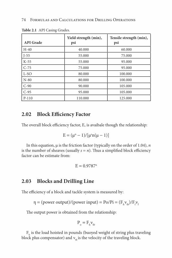
74 Formulas and Calculations for Drilling Operations
2.02 Block Efficiency Factor
The overall block efficiency factor, E, is avaibale though the relationship:
E (μn 1)/[μsn(μ 1)]
In this equation, μ is the friction factor (typically on the order of 1.04), n is the number of sheaves (usually s n). Thus a simplified block efficiency factor can be estimate from:
E 0.9787n
2.03 Blocks and Drilling Line
The efficiency of a block and tackle system is measured by:
η (power output)/(power input) Po/Pi (Fhν
tb)/F
fν
f
The output power is obtained from the relationship:
Po
Fhν
tb
Fh is the load hoisted in pounds (buoyed weight of string plus traveling
block plus compensator) and νtb
is the velocity of the traveling block.
Table 2.1 API Casing Grades.
API Grade
Yield strength (min),
psi
Tensile strength (min),
psi
H-40 40.000 60.000
J-55 55.000 75.000
K-55 55.000 95.000
C-75 75.000 95.000
L-SO 80.000 100.000
N-80 80.000 100.000
C-90 90.000 105.000
C-95 95.000 105.000
P-110 110.000 125.000

Rig Equipment 75
The input power from the draw works to the fast line is given by the relationship:
Pi
Ffν
f
Ff is the load in fast line, and v
f is the fast line speed. The relationship
between the travelling block speed and the fast line speed is:
vtb
νf/n
2.04 Crown Block Capacity
The crown block is the stationary section of a block and tackle that con-tains a set of pulleys or sheaves through which the drill line (wire rope) is threaded or reeved and is opposite and above the traveling block. The combination of the traveling block, crown block and wire rope drill line gives the ability to lift weights in the hundreds of thousands of pounds. On larger drilling rigs, when raising and lowering the derrick, line tensions over a million pounds are not unusual.
The crown block capacity required to handle the net static hook-load capacity can be calculated using the following formula:
Rc
[(HL
S)(n 2)]/n
where Rc is the required crown block rating (lbs), H
L is the net static hook-
load capacity (lbs), S is the effective weight of suspended equipment (lbs), and n is the number of lines strung to the traveling block.
Example calculationWhat minimum draw-works horsepower is required to drill a well using 10,000 ft of 4.5-inch OD 16.6# drill pipe and 50,000 lbs of drill collars? Efficiency is 65%.
Solution:
Drill string weight (air weight) 50,000 lbs(10,000 ft) (16.6 lb/ft) 216,000 lbs.
Hook horsepower [(216,000 lbs)(100 ft/min)]/33,000 655 hp.

76 Formulas and Calculations for Drilling Operations
Therefore, the required minimum draw-works horsepower rating655/0.65 1,007 hp
Please note that this neglects the effect of buoyancy and the weight of the block and hook.
2.05 Derrick Load
The static derrick load is calculated from the relationship:
Fs
[(n 2)/n] Fh
Dynamic fast line load is calculated from the relationship:
Ff
Fh/En
The dynamic derrick load is given by the relationship:
Ff
Fh
Fdl
The derrick load is calculated from the relationship:
Fd
[(1 E En)/En] Fh
The maximum equivalent derrick load is given asF
de[(n 4)/n] F
h
The derrick efficiency factor is calculated from the relationship:
Ed Fd/Fde
[E(n 1) 1]/[E(n 4)]
where Fdl
the dead line load.
Example calculationA rotary rig that handles triples is equipped with a 1200 hp draw-works. The efficiency of the hoisting system is 81%. Determine the time it takes to trip one stand of pipe at a hook load of 300,000 pounds.
SolutionThe efficiency of the system is:
η (power output)/(power input) Po/
Pi
0.81 Po/1200 and P
o927 hp

Rig Equipment 77
Since Po
νtb
/Fh
νtb
Po/F
h[927 33,000 (ft-lb/min)/hp]/300,000 102 fpm
and
t length/ νtb
90 ft/102 ft/min 0.84 min 50.5 sec
2.06 Energy Transfer
Efficiency transfer from the diesel engines to the mud pump can be given as in the Figure 2.1.
Due to interrelated equipment, various efficiencies can be used: (1) engine efficiency, η
e, (2) electric motor efficiency, η
el, (3) mud pump
mechanical efficiency, ηm
, and mud pump volumetric efficiency, ην from
which the overall efficiency is:
ηo
ηe
ηel
ηm
ην
Engine input (fuel energy) (1) engine output, i.e. input to pump, (2) mechanical pump output, i.e. input to hydraulic, and (3) hydraulic output
Power
input
(fuel
energy)
Power
output
(input to
pump)
Power
input Electric
motor
Power
output
Power
input
(mechanical)
Power
output
(mechanical)
Hydraulic
output
P,QDiesel
engine
ηe
ηo
ηv
ηm
ω
Figure 2.1 Energy Transfer.

78 Formulas and Calculations for Drilling Operations
Example calculationEstimate the liner size required for a double-acting duplex pump given the following pump details: (1) rod diameter 2.5 inches, (2) stroke length20-inch stroke, and (3) pump speed 60 strokes/min. The maximum avail-able pump hydraulic horsepower is 1,000 hp. For optimum hydraulics, the pump recommended delivery pressure is 3,500 psi.
Solution:The theoretical pump displacement for a duplex pump is:
Vi
π/4 NcL
s(2D
L2 D
R2) [2 20(2D
L2 2.52)]/294 gal/stroke
The theoretical flow rate of the pump operating at 60 strokes/min is:
Vt
[2 20(2DL
2 2.52)]/294 60 gal/stroke (16.33S
L2 51.02) gpm
The volumetric relationship is:
Qa
Qtn
υ
490 (16.33DL
2 51.02) 0.9 gpm
DL
6.03 inches
Therefore, the liner size that can be used is 6 inches.
2.07 Engine Efficiency
The overall efficiency of power generating systems can be calculated from the following relationship:
Efficiency (%) (output power)/(input power) 100
or
no
100(Pv/P
i)
The output power of an engine is:
Po
(2πNT)/33000

Rig Equipment 79
T output torque in ft-lbs, N engine rotary speed in revolution per minute (rpm), and P o output power in horsepower, hp. The input power is expressed as:
Pi
(QfH)/2545
Qf
rate of fuel consumption in lbm/hr, H fuel heating value in BTU/lb, and i input power in horsepower, hp. The fuel consumption can be calculated from:
Qf
48.46(NT/(ηH) lb/hr
2.08 Line Pull Efficiency Factor
Hoisting engines should have a horsepower rating for intermit-tent ser-vice equal to the required draw-works horsepower rating divided by 85% efficiency. Draw works also have a line pull rating efficiency depending on the number of lines strung between crown block and traveling block (Table 2.2).
Example calculationWhat line pull is required to handle a 500,000 lb casing load with 10 lines strung?
Solution
Line pull 500,000/(10) (0.81) 61,728 pounds
2.09 Mud Pump
A mud pump is a large reciprocating pump used to circulate the mud (drilling fluid) on a drilling rig. The pump uses a reciprocating piston/
Table 2.2 Effect of the number of Lines on Efficiency.
No. of lines Efficiency factor
6 0,074
8 0,042
10 0.811
12 0,782

80 Formulas and Calculations for Drilling Operations
plunger device that is designed to circulate drilling fluid under high pres-sure (up to 7,500 psi, 52,000 kPa)) down the drill string and back up the annulus.
2.09.1 Volume of Fluid Displaced
The following calculation can be used to determine the theoretical volume of fluid displaced:
For a single-acting pump:
Vt
[(π/4)DL
2Ls)]N
c
For a double-acting pump:
Vt
(π/4)NcLs)(2D
L2 D
r2)
The actual flow rate:
Qa
Qtη
v
The pump hydraulic horsepower is:
HHPp
(PpQ)/1714
DL
is the liner or piston diameter in inches, Ls is the stroke length in
inches, Nc is the number of cylinders, 2 for duplex and 3 for triplex, D
r is the
rod diameter in inches, and hv is the volumetric efficiency.
2.09.2 Volumetric Efficiency
The volumetric efficiency is determined using Qa, the actual flow speed:
ην
Qa/(displacement volume speed) 100
Thus:
ην
(Qt
ΔQ)/Qt
100
ΔQ is leakage losses and Qt is the theoretical flow rate which is equal to
the displacement volume multiplied by the pump speed.

Rig Equipment 81
2.09.3 Pump Factor
The pump factor is the pump displacement per cycle and is given as PF in bbl/stroke or gal/stroke.
The duplex pump factor is given by the relationship:
2(Vfs
Vbs
) PFd
PFd
(π/2)Ls(2D
L2 D
r2)
The triplex pump factor is given by the relationship:
3Vfs
PFt
PFt
(3π/4)DL
2Ls
The volumetric efficiency is given by the relationship:
ηv
(PFa)/(PF
t) 100
PFa is the actual pump factor, and PF
t is the theoretical pump factor.
For duplex pumps:
Vt
(π/4)NcL
s(2D
L2 D
r2)η
v
Vt
[NcL
s(2D
L2 D
r2) η
v]/(42 296) bbl/stroke
For triplex pumps (single-acting, three cylinders):
Vt
[Ls(D2) η
v]/(42 98.3) bbl/stroke
2.10 Offshore Vessels
Offshore vessels are ships that specifically serve operational purposes such as oil exploration and construction work on the oceans. There are a variety of offshore vessels, which not only help in exploration and drilling of oil but also for providing necessary supplies to the excavation and construc-tion units located on the oceans.

82 Formulas and Calculations for Drilling Operations
2.10.1 Terminology
The sides of offshore vessels and the types of vessel motions encountered are shown in Figure 2.2, Figure 2.3, and Figure 2.4.
Starboard
Aft
Port
Forward
Figure 2.2 Schematic of an Offshore Vessel.
Yaw
Heave
Surge
Sway
Pitch
Roll
Figure 2.3 Vessel Motion.
Depth of hullFreeboard
Beam
Draft
Figure 2.4 Vessel Draft and Freeboard.

Rig Equipment 83
In action, the depth of the vessel in the water (draft) and the distance above the water (freeboard) are also important factors.
2.10.2 Environmental Forces
Environmental forces that influence offshore vessels include: (1) wind force, (2) wave force, and (3) current force.
The wind force on an offshore vessel is calculated using the relationship:
Fw
0.00338Vw
2ChC
sA
In this equation, Fw is the wind force lbf, V
w is the wind velocity in knots,
Ch is the height coefficient, Cs is the shape coefficient, and A is the pro-
jected area of all exposed surface in squire feet. The shape coefficients and height coefficients can be estimated from the tables below:
The current force is calculated from the equation:
Fc
gcV
c2C
sA
Fc is the current drag force lbf, g
c V
c is the velocity of the current, C
s is
the drag coefficient and is the same as the wind coefficient, and A is the projected area of all exposed surfaces in square feet.
2.10.3 Riser Angle
The riser angle is measured relative to the vertical. Riser angles are mea-sured with respect to the and y axis, and the resultant riser angles follow.
Wind
Wave
Wind
Wave
CurrentCurrent
Mud line
Figure 2.5 Environmental Forces that Influence Offshore Vessels.

84 Formulas and Calculations for Drilling Operations
The equation is:
θ tan 1(tan2 θx
tan2 θy)1/2
Example calculationCalculate the percentage error in using the approximate equation to calcu-late the resultant riser angle when the riser angle in and y directions are 4° and 5°, respectively.
Solution:Using the equation above:
θ tan 1(tan2 θx
tan2 θy)1/2 tan 1(tan2 4 tan2 5)1/2 6.39°
Table 2.2 Shape Coefficients.
Shape Cs
Cylindrical shapes 0.5
Hull (surface type) 1.0
Deck House 1.0
Isolated structural shapes (cranes, beams..etc) 10
Under Deck areas (smooth surfaces) 10
Under Deck areas (exposed beams, girders) 13
Rig derrick (each face) 1.25
Table 2.3 Height Coefficients.
From to (ft) Ch
0–50 1.0
50–100 1.1
100–150 1.2
150–200 1.3
200–250 1.37
250–300 1.43
300–350 1.48
350–400 1.52
400–450 1.56
450–500 1.6

Rig Equipment 85
2.11 Rotary Power
Rotary horsepower can be calculated using the following equation:
Hrp
(2πNT)/33000
N is the speed of the rotary table in rpm and T is the torque in ft-lbs.
Example calculationIf a drill pipe has a maximum recommended make-up torque of 20,000 ft-lbs, then what is the rotary horsepower that can be transmitted at 100 rpm?
Solution:From the equation above:
Hrp
(2π 100 20,000)/33,000 381 hp
The empirical relationship to estimate the rotary horsepower require-ments is:
Hrp
F N
F is the torque factor in ft-lbf and N is the rotary speed in rpm. The torque factor (F) is generally estimated as follows: (1) F 1.5 to 1.75 for shallow holes less than 10,000 ft with light drill string, (2) F 1.75 to 2.0 for 10,000–15,000 ft wells with average conditions, (3) F 2.0 to 2.25 for deep holes with heavy drill string, and (4) F 2.0 to 3.0 for high-torque.
The above empirical estimates are subject to many variables but have proved to be reasonable estimates of rotary requirements. However, for highly deviated wells, torque/H
rp requirements must be closely calculated
using available computer software programs.
2.12 Ton-Miles Calculations
2.12.1 Round-Trip Ton Miles Calculations
Tf [(Lh
Ls)W
dp4L
h(Wb 0.5W
10.5W
2
0.5W3)]/10,560,000 ton-miles

86 Formulas and Calculations for Drilling Operations
where Lh
is the measured depth of the hole or trip depth in feet, Ls is the
length of the stand in feet, Wdp
is the buoyed weight of the drill pipe per foot, ppf, W
b is the weight of the block, hook, etc. in pounds, W
1 is the
excess weight of drill collar in mud, lbs (buoyed drill collar weight in mudbuoyed drill pipe weight of same length in mud), W
2 is the excess weight of
heavy weight pipe in mud, lbs (buoyed heavy weight pipe in mud buoyed drill pipe weight of same length in mud), and W
3 is the excess weight of
miscellaneous drilling tools in mud, lbs (buoyed miscellaneous drilling tools in mud buoyed drill pipe weight of same length in mud).
2.12.2 Drilling Ton-Miles Calculations
When a hole is drilled only once without any reaming, the relationship is:
Td
2(Ti + 1
Ti)
When a hole is drilled with one-time reaming, the relationship is:
Td
3(Ti + 1
Ti)
When a hole is drilled with two times reaming, the relationship is:
Td
4(Ti + 1
Ti)
Ti is the round-trip ton-mile calculated from depth i.
2.12.3 Coring Ton-Miles Calculations
Td
2(Ti + 1
Ti)
2.12.4 Casing Ton-Miles Calculations
Tf
0.5[Lh(L
sL
h)W
c4W
bL
h)/10,560,000
Wc is the buoyed weight of the casing per foot.
Example calculationCalculate the ton-mile for a round trip from 8,000 feet with 450 feet of drill collar with a weight of 83 ppf. The weight of the drill pipe is 19.5 ppf. The

Rig Equipment 87
mud density is 9.6 ppg. Assume the stand length to be 93 feet and the total block weight is 40,000 lbs.
Solution:From the equation above, L
h is 8000 ft, L
s is 90 ft, and W
b is 40000 lbs. The
buoyancy factor is 0.853 (i.e., 1 9.6/65.5).
Wdp
19.5 0.853 16.64 ppf.
The (buoyed weight of drill collar) minus (the buoyed weight of drill pipe) 0.853 450(83 19.5) 24,387 lbs.
Thus:
Tf
[8000(93 8000)16.64 4 8000(4000024387)]/10,560,000 297 TM.

89
3.01 Average Curvature-Average Dogleg Severity
The equations used to calculate the average curvature of a survey interval are:
k [(Δα/ΔL)2 (Δφ/ΔL) 2 sin2 α)]1/2
k β/ΔL
In these equations, α is the inclination (in degrees), φ is the azimuth or direction in degrees, ᾱ is the average inclination angle (in degrees), k is the average borehole curvature, and β is: acos(cosα
1cosα
2sinα
1sinα
2cosΔφ).
3.02 Bending Angle
Using the inclination angles and directions, the borehole beding angle is derived from the following equation:
cos β cosα1cos
2sin
1sin
2cosΔφ
3Well Path Design
Formulas and Calculations for Drilling Operations, Second Edition.James G. Speight.
© 2018 Scrivener Publishing LLC. Published 2018 by John Wiley & Sons, Inc.

90 Formulas and Calculations for Drilling Operations
Δφ is equal to φ2 φ
1, β is the bending angle in degrees, Δφ is the section
increment of azimuth angle in degrees, α1 is the inclination angle at survey
point 1 in degrees, and α2 is the inclination angle at survey point 2 in degrees.
3.03 Borehole Curvature
3.03.1 General Formula
Borehole curvature is derived by using the general formula:
k (kα
2 kϕ2 sin2α)1/2
In addition, the general formula for borehole curvature with the vertical and horizontal curvatures can be is:
k (kv
2 kH
2 sin4α)1/2
κv is the curvature of wellbore trajectory in a vertical expansion plot in
degrees/30 meters or in degrees/100 feet, and κH
is the curvature of well-bore trajectory in a horizontal projection plot in degrees/30 meters or in degrees/100 feet.
3.03.2 Borehole Radius of Curvature
The borehole radius of curvature and torsion can be determined by use of either of two formulas:
R (180Ck)/(πk)
ρ (180Ck)/(πτ)
Cκ
is the constant related to the unit of borehole curvature. If the unit for borehole curvature is degrees/30 meters and degrees/100 feet, then C
κ
is equal to 30 and 100, respectively.Κ is the curvature of wellbore trajectory in degrees/30 meters (or
degrees/100 feet) and τ is the torsion of wellbore trajectory in degrees/ 30 meters (or degrees/100 feet).
Example calculationCalculate the radius of curvature for a buod section with a build rate of 2 degree per 100 feet.

Well Path Design 91
SolutionUsing the first of the two equations presented in this sub-section, the radius of curvature is:
R (180Ck)/(πk)
Ck
100
Thus, the radius of curvature, R, is:
R (180 100)/π2 2,863.63 feet
3.04 Borehole Torsion
3.04.1 General Method
The borehole bending angle can be derived using the following equation:
τ (kαk
ϕk
ϕk
α/k2) sin α k
ϕ(1 k
α2/k2)cos α
τ is the torsion of wellbore trajectory in degrees/30 meters or in degrees/100 feet, k
α is the first derivative of inclination change rate, viz., the second
derivative of inclination angle, and φ is the first derivative of azimuth change rate, viz., the second derivative of azimuth angle.
3.04.2 Cylindrical Helical Method
When the wellbore curvature equals zero, the wellpath is a straight line that will result in zero torsion. When κ is not equal to zero, the torsion equation for the cylindrical helical model is:
τ kH[1 (2k
v2)/k2]sinα cosα
Example calculationIf the original hole inclination is 22o, to reach the limits of the target, it is desired to build an angle of 26° in a course length of 100 feet and the direc-tional change is 5°. What is the resulting curvature and torsion that will achieve the desired objective?

92 Formulas and Calculations for Drilling Operations
SolutionSince α
122°; α
226°; Δφ − 5°; k
α4°/100 ft; k
φ7°/100 ft, and ΔL
100 feet, the vertical curvature is:
kα
(α2
α1)/L
2L
1) 4/100 100 4° per 100 feet
The average inclination angle is:
ά= (α1
α/2) (22 26)/2 24°
kα
kv
4o per 100 feet
kH kϕ/sinα 10/sin24 12.294° per 100 feet
The wellbore curvature can be calculated as:
k (kv
2 kH
2 sin4α)1/2 4.487° per 100 feet
The torsion is calculated as:
τ 12.294[1 (2 42)/4.4872]sin24cos24 11.827° per 100 feet
3.05 Horizontal Displacement
On the horizontal plane, the displacement of the target point can be calcu-lated from the equation:
Ht
[(Nt
No)2 E
tE
o)2]1/2
Nt is the distance northing of target (i.e. the refers to the northward-
measured distance) in feet, ft, No is the distance northing of the slot in feet,
Et is distance easting of target (i.e. the refers to the eastward-measured dis-
tance) in feet, and Eo is the distance easting of slot in feet.
The target bearing is given as:
Φt
tan 1(Et
Eo)/N
tN
o)
Example calculationWith the slot coordinates 1200.5 ft N, 700 ft E and target coordinates 3800 ft N, 4520 ft E, calculate the horizontal displacement of the well. Also, cal-culate the target bearing.

Well Path Design 93
SolutionSince N
t3800 ft, N
o1200.5 ft, E
t4520 ft, and 700 ft The horizontal
displacement is:
Ht
[(3800 1200.5)2 (4520 700)2]1/2 4620.6 ft
The target bearing is:
φt
tan 1[4520 700)/3800 1200.5)] 55.76° or N55.76E
3.06 Magnetic Reference and Interference
Declination (Figure, below) is the angular difference in azimuth readings between magnetic north and true north. Magnetic declination is positive when magnetic north lies east of true north, and it is negative when mag-netic north lies west of true north. It is the error between the true north and magnetic north for a specific location.
Azimuth correction can be given as:
Azimuth (true) Azimuth (magnetic) Magnetic declination
For westerly declination, the azimuth correction is:
Azimuth (true) Azimuth (magnetic) ( Magnetic declination)
Magnetic north
Declinattion
True north
Magnetic northTrue north
+ve
–ve
SS
Figure Declination/East-West Declination.

94 Formulas and Calculations for Drilling Operations
3.07 Tool Face Angle
With the inclination angles and directions, the tool face rotation is derived from the equation:
γ arc cos[(cos α1 cos β cos α
2)/(sin α
2 sin β)]
Example calculationCalculate the dogleg severity from the following date:
For true North and grid North, true north uses latitude and longitude coordinates of the curved earth as the reference. Longitudes converge upon the rotational pole. In the grid system, the Y-axis does not converge to single point.
Magnetic Declination Grid Convergence Total Correction
Magnetic Azimuth Total Correction Corrected Azimuth
Example calculationDetermine the azimuth with respect to the true north of the following wells:
1. N45E, declination 5 degrees west,2. N45E, declination 5 degrees east.
Solution1. Azimuth 45 5 40 degrees N40 E,2. Azimuth 45 5 50 N50 E (as shown below).
40
E E
S
455
50
S
45
5
True north True azimuthMagnetic
northTrue north True azimuth
Magnetic
north

Well Path Design 95
Measured depth (ft) Angle (degrees) Direction (degrees)
15000 16.5 150
15045 17.5 148
arccoscos . cos . cos .
sin . sin ..
2 01 5 5 7 5
7 5 2 0143 2770 .
Problem 3.8While drilling a directional well, a survey shows the original inclination of 32 deg and an azimuth of 112 deg. The inclination and directional curvatures are to be maintained at 4 deg/100 ft and 7 deg/100 ft, respectively, for a course length of 100 ft. Calculate the new inclination angle and final direction. Also, determine the curvature, vertical curvature, and horizontal walk curvatures.
Solution:Given data: a 32 deg; <t>2= 112 deg; 4 deg/100 ft; v =7 deg/100 ft; AL 100 ft
The new inclination angle is
2 1 2 1 324
100100 36a L L .
The new direction is
2 1 2 1 1127
100100 119L L .
The average inclination angle is
1 2
232 36
234
The average curvature is
4 7 34 5 596 1002 2 2sin . / .ft
Using the bending or dogleg angle,
cos cos cos sin sin cos ,1 2 1 2
k ftarc cos cos cos sin sin cos
. / .32 36 32 36 7
1005 591 100

96 Formulas and Calculations for Drilling Operations
It can be seen that a small difference is observed between the two calcu-lation methods.
Vertical curvature is
v a ft4 100/ .
Horizontal curvature is
H ft7
3412 518 100
sin. / .
3.08 Tool Face Angle Change
If the inclination α, new inclination αn, and the dogleg severity β are
known, then the tool face angle can be calculated using the following relationship:
γ arc cos[(cos α cos β cos αn)/(sin α sin β)]
If the new inclination αn, azimuth change Δφ, and the dogleg severity b
are known, then the tool face angle can be calculated using the following relationship:
γ arc sin[(sin αn sin Δβ)/(sin β)]
If the inclination α, the dogleg severity β, and the toolface angle g are known, the new inclination angle can be calculated using the following relationship:
αn
arc cos(cos α cos β sin β sin α cos γ)
If the inclination α, the dogleg severity β, and the tool face angle γ are known, the change in the azimuth can be calculated using the following relationship:
Δφ arc tan[(tan β sin γ)/sin α tan β cos α cos γ)]
Example calculationDerive an equation to find the overall angle change in terms of Δφ, α, and γ, the tool face rotation angle.

Well Path Design 97
SolutionStarting from the azimuth change:
Δφ arc tan(tan β sin γ)/sin α tan β cos αcos γ)
tan Δφ (tan β sin γ)/sin α tan β cos α cos γ)
Thus:
tan Δφ sinα tanβ(tan Δφ cos α cos γ-sin γ) 0
This leads to an equation for the overall angle change, β
Β β arc tan[(tan Δφ sin α)/(sin γ-tan Δφ cos α cos)]
3.09 Tortuosity
Tortuosity is a property of a curve being tortuous (twisted; having many turns) and there have been several attempts to quantify this property. Wellbore tortuosity is derived from the equation:
T
D
D D
n ii t
m
i i
1
1
.
3.09.1 Absolute and Relative Tortuosity
The equation is:
( ) ,abs
adji
i
n nD D1
1
In this equation, αadj
ai
ΔDi
bi and is the dogleg adjusted, summed
total inclination angle.
( ) ( ) ( ) deg/ .rel abs
tar
abs
notar ft100

98 Formulas and Calculations for Drilling Operations
The period of the sine wave should not be of 2/n (n 1, 2, 3…)Different methods include (1) the sine wave method, (2) the helical
method, (3) random inclination and the azimuth method, and (4) the random inclination dependent azimuth method.
3.09.2 Sine Wave Method
Δα sin (D/P 2π) M
D is the measured depth in feet, P is the period, and M is the magnitude. If the measured depth of the survey point is an exact integer multuiple of the period, then:
Δα sin (MD/P 2π) 0
In addition, the inclination angle is modified so that it does not become less than zero, since negative inclination angles are not allowed.
If the Δα term is negative and φ φn
Δα is negative, then φn
360Δα, then:
αn
α Δα
φn
φ Δα ψxvc
ψxvc
is the cross vertical correction.If α
n0, the cross vertical correction 180o or if α
n0 the cross vertical
correction 0o.
Example calculation
Measured depth 3900 ft, Inclination 5.15°, and Azimuth 166°.
Measured depth 3725 ft, Inclination 3.25°, and Azimuth 165°.
Calculate the tortuosity using the sine wave method.
Solution:
Δα sin (3725/1000 2π) 1 0.99°
φn
165 0.99 0 164.1°
αn
3.25 0.99 2.26°

Well Path Design 99
3.09.3 Helical Method
The helical method modifies the inclination and azimuth of the survey points by superimposing a helix along the wellbore path using the magni-tude (radius of the cylinder in the parametric equation) and period (pitch) specified. This method uses the circular helix defined as: f(u) a cos(u)a sin(u) bu.
The generalized parametric set of equations for the helix used to super-impose the wellbore path is given by:
x u M u
y u M u
z uP
u
( ) cos( )
( ) sin( )
( )2
3.09.4 Random Inclination Azimuth Method
αn
α Δα
φ φn
Δα ψcvc
As above, ψcvc
is the cross vertical correction.
Example calculation
Measured depth 3725 ft, Inclination 3.25°, and Azimuth 165°.
Measured depth 3900 ft, Inclination 5.15°, and Azimuth 166°.
ζ (Rand number) 0.375.
Calculate the tortuosity using the random inclination azimuth method.
Solution:
Δα [0.375 (3900 3725/100)] 1 0.66o
αn
5.15 0.66 5.81o
φn
166 0.66 0 166.66o

100 Formulas and Calculations for Drilling Operations
3.09.5 Random Inclination Dependent Azimuth Method
Δα ζ δ
δ (ΔMD/P)M
ζ is the random number, αn
α Δα
φn
φ [Δα/(2 sin αn)] ψ
cvc
Example calculation
Measured depth 3725 ft, inclination 3.25°, and azimuth 165°.
Measured depth 3900 ft, inclination 5.15°, and azimuth 166°.
Random number 0.375.
Calculate the tortuosity using the random inclination dependent azi-muth method.
Solution:
Δα [0.375 (3900 3725)]/100 1 0.66o
αn
5.15 0.66 5.81o
φn
166 +(0.66/2 sin 5.81) 0 169.26o
3.10 Types of Wellpath Designs
The different types of Wellpath designs are shown in Figure (below):
3.11 Vertical and Horizontal Curvatures
Vertical and horizontal curvatures can be calculated using the following equations:
κv
κα
κv
dα/dL κα

Well Path Design 101
κH
κφ/sin α
κH
dφ/dS dφ/(dL sin α) κφ/sin α
kV is the curvature of the wellbore trajectory in a vertical position plot in
degrees per 30 meters or degrees per/100 feet, kH
is the curvature of the wellbore trajectory in a horizontal projection plot, degrees per 30 meters or degrees per 100 feet, dL L
2L
1 and is the curved section length in meters
or feet, and S is the arc length in the azimuthal direction in meters or feet.
3.12 Wellbore Trajectory Uncertainty
Nominal distance between two points, i.e., from the point concerned in a reference wellbore (the reference point) to the point observed in the object wellbore (the object point), is:
Sor
[(xo
xr)2 (y
ot
r)2 (z
oz
r)2]1/2
0
200 E
Undercut
S-Type
J-Type
S-Tum
Horizontal
Extended reach
N
O
H
400
600
800
1000
1200
1400
1600
1800
2000
2200
–600–400 –200 0 200 400 600 800 1000 1200
–600–800
–400–200
0200
400600
8001000
1200
Figure 3.1 Wellpath Designs.

102 Formulas and Calculations for Drilling Operations
Reference well
Offset well
Xr, Yr, Zr
X0, Y0, Z0
Figure 3.2 Reference and Offset Well.
In this equation, xo, y
o, and z
o are coordinates of the object point in the
OXYZ system and xr, y
r, and z
r are coordinates of the object point in the
OXYZ system Sor
(Figure).If rs represents the sum of the radii, then:
rs
ro
rr
where ro is the radius of an object well and r
r is the radius of a reference
well. The relative covariance of the matrices are:
ΣRR
ΣPoPo
ΣRrPr
ΣPoPo
and ΣRrPr
are the covaroaince matricies of the points Po ands P
r,
respectively. The azimuth and dip angle of the single point can be deter-mined by:
φ arc sin [Ur2 V
r2)/S
or] and θ arc tan V
r/U
r
If kp is the amplifying factor corresponding to an ellipsoid on which the
signal point lies, it is given by:
k DS/(σ1
2cos2θsin2ϕ σ2
2sin2θsin2ϕ σ3
2cos2ϕ
In this equation, ϕ is the azimuth angle and θ is the dip angle.

Well Path Design 103
3.13 Wellpath Length Calculations
Circular arc:
Arc length Lc
(α1
α2)BRA
BRA is the build rate angle in degrees per 100feet.Vertical distance is given by:
V Rb(sin α
2sin α
1)
Rb is the radius of the build or:
Rb 180/(π BRA)
Horizontal distance, H, is given by:
H Rb(cos α
1- cos α
2)
Tangent section:
Length of tangent Lt
Vertical distance V Lt cos α
Horizontal distance H Lt sin α
Example calculationDetermine the build rate radius from the data for a build-and-hold pattern type well: build rate angle 30 degrees per w00 feet.
Solution
Rb
1/BRA(180/π) 100/3(180/π) 1910 feet.

105
4Fluids
4.01 Acidity-Alkalinity
Acidity or alkalinity is expressed as the pH of the material or solution (Table 4.1).
The pH is the negative logarithm of [H+] or [OH–] and is a measurement of the acidity or alkalinity of a solution:
pH = log([H+])
pH = log([OH−)]
[H+] or [OH–] are hydrogen and hydroxide ion concentrations, respec-tively, in moles/liter. Also, at room temperature, pH pOH = 14. For other temperatures: pH pOH = pKw, where Kw = the ion product constant at that particular temperature.
Formulas and Calculations for Drilling Operations, Second Edition.James G. Speight.
© 2018 Scrivener Publishing LLC. Published 2018 by John Wiley & Sons, Inc.

106 Formulas and Calculations for Drilling Operations
Example calculationAn aqueous potassium hydroxide completion fluid has a pH of 9. Determine the hydrogen ion concentration of this solution?
Solution:From the pH equation (abpove):
pH = −log([H+])
The hydrogen ion concentration is:
[H+] = 10−pH = 10 10 = 1 × 10⁻⁹ mol/L (10−9 M).
4.02 Base Fluid–Water-Oil Ratios
The base fluid/water ratio can be calculated as the percentage by volume of base fluid in a liquid phase:
Pb = VR
b/(VR
b + V R
w) 100
VRb is the volume percent of base fluid and VR
w is the volume percent
of water. The percent of water is Pw = 100 P
b
Example calculationIf the base fluid is 62%, water is 12%, and solids is 26%, calculate the base fluid-water ratio.
Pb = VR
b/(VR
b + V R
w) 100 = 62/(62 + 12) 100 = 83.78
Pw = 100 P
b = 100 83.78 = 16.22
Pb/P
w = VR
b/VR
w = 83.78/16.22 = 5.17
Table 4.1 Ranges of Acidity and Alkalinity.
pH [H ] Solution
<7 > 1.0 10−7 M Acid
>7 < 1.0 10−7 M Basic
7 = 1.0 10−7 M Neutral

Fluids 107
4.03 Common Weighting Materials
A weighting material is a high-specific gravity and finely divided solid material that is used to increase the density of a drilling fluid. Barite is the most common weighting material as is hematite (the mineral form of ferric oxide, Fe
2O
3). Calcium carbonate, specific gravity is also a weighting mate-
rial but is used more for its acid solubility than for density modification. The average weights of the commonly used weighting materials are
given in the Table 4.2 (below). Table 4.3 and Table 4.4 (below) provide general size range (in microns) of a variety of solids.
Table 4.2 Common Weighting Materials.
Weighting materials
Specific gravity
(gm/cm3)
Density (lbm/
gal ppg)
Density (lbm/
bbl ppb)
Barite Pure grade 4.5 37.5
Barite API – drilling rade 4.2 35 1,470
Bentonite 2.6 21.7 910
Calcium carbonate 2.7 22.5 945
Calcium chloride 1 .96 16.3 686
Sodium chloride 2.16 18 756
Water J 8.33 1,001
Diesel 0.86 7.2 300
Iron oxide 5 41.73 5,005
Galena 6.6 55 6,007
Drilled solids 2.7 21.7 2,702
Table 4.3 Micron sizes.
Mineral Micron size
Clay <1
Bentonite <1
Barite 2–60
Silt 2.74
Sand >74

108 Formulas and Calculations for Drilling Operations
Example calculationDetermine the percentage of clay based on a ton (2000 lb) of clay of 10 ppg clay-water drilling mud. The final mud volume is 100 barrels.
Solution:If X is the percentage of clay in the final mud, then:
X/100 ρf V
f = 2000
X/100 10 500 = 2000
Therefore:
X = 2000/(10 100 42) 100 = 4.76%
4.04 Diluting Mud
The dilution process involves selective dumping of the active system (such as sand traps and bottoms-up mud) and replacement of the lost volume with fresh mud. This process has proved economical with inhibitive water-base systems and is the only method that actually removes colloidal-size particles.
When diluting mud with a liquid, the resulting density of the diluted mud can be derived from:
ρf = ρ
o + V
a/V
o(ρ
o ρ
a)
ρo is the original mud weight, ppg, V
a is the original volume in barrels, V
o
is the final volume in barrels, and ρa is the density of material added, ppg.
Example calculationDetermine the final mud density of mud if 100 barrels of diesel with a specific gravity of 0.82 are mixed with 500 barrels 9 ppg mud.
Table 4.4 Micron Cut Points for Solid Removal Systems.
Equipment Micron size
Centrifuge 3 to 5
Desilter (3 to 4-inch cones 12 to 60
Desander (5 to 12-inch cones) 30 to 60

Fluids 109
Solution:The final volume of mud after adding diesel = 500 + 100 = 600 bbl. Using the density relationship, the final density of the mud can be derived from:
ρf = [9 + (100/6)](9 0.82 8.33) = 8.57 ppg
4.05 Drilling Fluid Composition
A drilling fluid (also called drilling mud) is a fluid that is used to aid the drilling of of crude oil and natural gas. The three main categories of drilling fluids are water-based muds (which can be dispersed and non-dispersed), non-aqueous muds, usually called oil-based mud, and gaseous drilling fluid, in which a wide range of gases can be used.
Element Water Cuttings Barite Clay
Chrome-
ligno-
sulfonate Lignite Caustic
Aluminum 0.3 40,400 40,400 88,600 6,700 6,700 0.013
Arsenic 0.0005 3.9 34 3.9 10.1 10.1 0.039
Barium 0.01 158 590.000 640 230 230 0.26
Calcium 15 240,000 7,900 4,700 16,100 16.100 5,400
Cadmium 0.0001 0.08 6 0.5 0.2 0.2 0.0013
Chromium 0.001 183 183 8.02 40.030 65.3 0.00066
Cobalt 0.0002 2.9 3.8 2.9 5 5 0.00053
Copper 0.003 22 49 8.18 22.9 22.9 0.039
Iron 0.5 21.900 12,950 37,500 7.220 7.220 0.04
Lead 0.003 37 685 27.1 5.4 5.4 0.004
Magnesium 4 23,300 3,900 69,800 5,040 5,040 17.800
Mercury 0.0001 0.12 4.1 0.12 0.2 0.2 5
Nickel 0.0005 15 3 15 11.6 11.6 0.09
Potassium 2.2 13,500 660 2,400 3.000 460 51.400
Silicon 7 206,000 70,200 271.000 2,390 2,390 339
Sodium 6 3,040 3.040 11,000 71.000 2,400 500.000
Strontium 0.07 312 540 60.5 1030 1030 105

110 Formulas and Calculations for Drilling Operations
4.06 Equivalent Mud Weight
On a theoretical basis, the equivalent mud weight and the hydrostatic pres-sure are the same if the borehole is free of cuttings. Typically, the borehole is not free of cuttings and the annular pressure sensor is used to provide an accurate downhole pressure reading used to calculate equivalent mud weight (EMW). However, the true vertical depth (TVD) must be correct to effectively use the equivalent mud weight to make real-time drilling decisions.
Thus, the pressure in the wellbore or formation can be expressed in terms of equivalent mud weight (EMW), which is a convenient way to compare the pressures at any depth.
EMW (ppg) = Ph/(0.52 L
tvd)
Ltvd
is the true vertical depth (TVD) in feet, and Ph is the annular pres-
sure in psi. If the well is deviated α degrees from the vertical, then:
EMW (ppg) = Ph/(0.52 D
h cos α)
Dh is the measured depth in feet.
4.07 Fluid Loss
The volume fraction of solids in mud, fvm
, can be written as
fvm
= Vs/V
m = f
vc + hA/(V
f + hA)
Vf is the amount of filtrate volume, h is the cake thickness, A is the filtra-
tion area, Vm
is the total volume of mud filtered, and Vs is the volume of
solids deposited in mud cake. The API water loss is derived from:
V30
= V7.5
Vsp
Filter loss is always estimated with reference to the square root of time. Filtrate volume is derived from:
Vf = A[2k(f
vc/f
vm 1)ΔPt/μ]1/2 + V
s

Fluids 111
where ΔP is the differential pressure, μ is the filtrate viscosity, t is the filtra-tion time, and k is the cake permeability.
Example calculationThe spurt loss of a mud is known to be 2 cc. If a filtrate of 10 cc is collected in 15 minutes using a filter press, what is the standard API filtrate for this mud?
Solution:The filter loss at 7.5 minutes is found by extrapolating the data given at time zero and fifteen minutes. Thus, if X is the filter loss at 7.5 minutes:
2 = (10 X)(151/2 7/51/2) 7.51/2
Thus:
V30
= 2V7.5
Vsp
= 2 6.69 10 =3.38 cc
Let x be the filter loss at 7.5 minutes. So, the filter loss at time 7.5 minutes is
210
15 7 57 5
x
..
Solving for will yield 6.69 cc.Using equation 4.29, API filter loss is
V V V ccsp30 7 52 2 6 69 10 3 38. . . .
Problem 4.32A kick was taken at 10000’ while drilling with a 14 ppg mud. Stabilized shut-in drill pipe pressure = 600 psi. Determine the amount of barite to be added to 800 bbl of original mud in order to contain formation pres-sure such that a differential pressure of 300 psi is achieved after killing the well.
Solution:Equivalent mud weight needed to control the kick with the excess differ-ential pressure is
600 0 052 14 10000 7280 300
0 052 1000015 73
. ( )
.. .

112 Formulas and Calculations for Drilling Operations
The amount of barite required is
mg 42 28 0215 73 14
28 02 15 73132593.
.
. . lbm.
Assuming 100 lbm per sack, the number of sacks of barite required is 1325.
4.08 Marsh Funnel
The Marsh funnel is a device for measuring viscosity by observing the time it takes a known volume of liquid to flow from a cone through a short tube. It is standardized for use by mud engineers to check the quality of drilling mud. As a standard reference point, the time for fresh water to drain = 26 sec ± 0.5 sec per quart for API water at 70°F ± 0.5°F.
The effective viscosity can be determined from following simple formula:
μ = ρ (t 25)
where μ is the effective viscosity in centipoise, ρ is the density in g/cm3, t is the quart funnel time in seconds.
For example, a mud of funnel time 40 seconds and density 1.1 g/cm3 has an effective viscosity of about 16.5 cP. For the range of times of typical muds above, the shear rate in the Marsh funnel is about 2000−s.
4.09 Mud Rheology
Rheological properties of drilling fluid have considerable impact on car-rying out of drilling cutting on a day surface, creation of hydrodynamic pressure in well. In terms of mud rheology, the shear stress (τ) and shear rate (γ) for Newtonian fluid are given as:
τ = μγ
μ is the Newtonian viscosity. In engineering units, τ is dynes/cm2 = 4.79 lb/100 feet2, γ = sec−1, and
μ = poise = dyne × sec/cm2. The field unit of viscosity is the centipoise (1 poise = 100 centipoise) and the field unit of shear stress is lb/100 ft2.

Fluids 113
For the Bingham plastic model, the relationship is given by the equation:
τ = τy +μ
pγ
For the power law model, shear stress (τ) and shear rate (γ) are given by the equation:
τ = Kγn
Shear rate and shear stress relationship for various fluids are presented in Figures 4.1, 4.2, and 4.3.
Pseudo-plastic shear thinning
Newtonian fluid
Real plastic
Shear-thickening
Sh
ea
r st
ress
τ –
lbf/
10
0 f
t2
Shear rate γ – sec–1
Figure 4.1 Shear Rate-Shear Stress Relationship of Time Independent Non-Newtonian
Fluids.
Bingham plastic fluid
Slope = Plastic viscosity
Yield power law fluidReal plastic
Power law fluid
Yield point
Sh
ea
r st
ress
τ –
lbf/
10
0 f
t2
Shear rate γ – sec–1
Figure 4.2 Shear Rate-Shear Stress Relationship of Non-Newtonian Fluids.

114 Formulas and Calculations for Drilling Operations
For the yield power law (Herschel Bulkley), shear stress (τ) and shear rate (γ) are given by the equation:
τ = τy + Kγ
n
τy is the yield value or yield stress, μ
p is the Bingham plastic viscosity, K
is the consistency index, and n is the power law index.
4.10 Mud Weighting
Mud weighting is the addition of a high-density material such as barite to increase the mud weight (mud density)
The four fundamental equations used in developing mud weight-ing mathematical relations are (1) the material balance equation, (2) the volume balance equation, (3) the relationship between weight and vol-ume equation, and (4) the volume balance in low specific gravity solids equation:
Wf = W
o + W
a
Lo
g s
he
ar
stre
ss τ
Log shear rate γ
Slope = n
Intercept – K
Figure 4.3 Shear Rate-Shear Stress Relationship of a Power Law Fluid Using the
Logarithmic Scale.

Fluids 115
Wf = W
o + W
a are the final mixture weight, original liquid weight, and
added material weight, respectively. Thus:
Vf = V
o + V
a
Vf, V
o, and V
a are the final mixture volume, original liquid volume, and
added material volume, respectively.
ρ = W/V
where ρ, W, and V are the weight density, weight, and volume, respectively.
Vff
vf = V
of
vo
where fvf and f
vo are the volume fraction of low specific gravity solids in the
final mixture and in the original liquid, respectively. The above equations may be combined and rearranged algebraically to
suit the calculations desired. Thus:
V1ρ
1 + V
2ρ
2 + V
3ρ
3 + V
4ρ
4 + … = V
fρ
f
V1 + V
2 + V
3 + V
4 + … = V
f
V1 + V
2 + V
3 + V
4 are the volumes of materials 1, 2, 3, and 4, respectively,
and ρ1, ρ
2, ρ
3 and ρ
4 are the densities of materials 1, 2, 3, and 4, respectively.
A simultaneous solution of the two equations above results in any two sought unknowns and the rest of the parameters are known. The following are example formulations for commonly encountered field problems:
1. The amount of weighting materials required to increase original mud density, ρ
o, to a final density, ρ
f, is
Wwm
= 42(ρf ρ
o)/(1 ρ
f /ρ
wm)
Wwm
is the required amount of weighting material, lbs/bbl, or original mud.
2. The average weight density, ρav
, of two added materials i and j of weights ρ
i and ρ
j, respectively, is:
ρav
= ρiρ
j/f
wf
i + (1 + f
w) ρ
j

116 Formulas and Calculations for Drilling Operations
where fw = w
j/w
i + w
j is the weight fraction of material j with
respect to added weights of materials i and j. 3. The amount of liquid volume, V
l, required to make a mud of
total volume Vf having a weight of ρ
f is:
Vl = V
f[(1 ρ
f/ρ
a)/(1 ρ
l/ρ
a)]
where ρa is the weight density of added material or average
weight density, ρav
, of material added to the liquid. 4. The amount of solids i and j, such as clay and barite for
example, required to make-up a specified final mud volume, V
f, and density, ρ
f, is:
wi = 42fw(ρ
fρ
o)/1 (ρ
o/ρ
j) (1 f
w)(ρ
oρ
i)
wj = ( 1 fw)(ρ
o ρ
j)/1 (ρ
o/ρ
j) (1 f
w)(ρ
oρ
i)
where wi and w
j are the solid materials i and j in lbs/bbl of
final mud. 5. The final mud density, ρ
f, when a certain liquid volume, V
l,
of density ρl is added to a mud system of original density, ρ
o,
and volume, Vo, is:
ρf = (ρ
o + αρ
1)/(1 + α)
where α = Vl/V
o.
4.11 Plastic Viscosity, Yield Point, and Zero-Sec Gel
4.11.1 Bingham Plastic Model
Plastic viscosity, yield point, and zero-sec-gel can be calculated from the Fann reading using the following relationships:
PV = 600
− 300
YP = 2300 600
τ = 3

Fluids 117
Alternatively, the dial readings can be reverse calculated by using PV, YP, and zero-gel. Thus:
300 = PV + YP
600 = 2PV + YP
3 = τ
0
600 is the Fann dial reading at 600 rpm,
300 is the Fann dial reading at
300 rpm, and 3 is the dial reading at 3 rpm. If the Fann RPMs are anything
other than 600 rpm and 300 rpm, the following relationship can be used:
μp = 300/(N
2 N
1)/(
N1 N2)
4.11.2 Shear Stress and Shear Rate
Shear stress and shear rate can be calculated using the following relationships:
τ1 = (0.01065) lbf/ft2
τ2 = (1.065) lbf/100 ft2
γ = (1.073) N 1/sec
N is the dial speed in 1/sec.
4.11.3 Power Law
The rheological equation for the power law model can be given as:
τ = Kγn
where γ is the shear rate (1/sec) and τ is the = the shear stress (1b/ft2). The flow behavior index can be given as:
n = 3.322 log (600
/300
)
For the modified power law, the equation is:
n = 3.322log (YP + 2PV)/(YP + PV)
PV is the plastic viscosity and YP is the yield point.

118 Formulas and Calculations for Drilling Operations
The consistency index, K, is given as:
K = (510300
)/511n eq. cP
K can be expressed in (lb × secn/ft2) using the conversion factor:The consistency index, K, for the modified power law is given as:
K = (YP + 2PV)/[(100)(1022n)
If the Fann RPMs are anything other than 600 and 300, the following relationship can be used:
n = (log N2
/N1
)/(log N2/N
1)
4.12 Reynolds Number and Critical Velocity
In fluid mechanics, the Reynolds number (Re) is a dimensionless quantity that is used to help predict flow patterns in different fluid flow situations. The Reynolds number is used to predict the transition from laminar flow to turbulent flow.
The Reynolds Number, used in the annular Power Law Model calcula-tions is calculated using equivalent viscosity (m):
Μ = [90000 Pla (d
1 d
2)2]/(L V)
The Reynolds Number is then:
Re = [15.47 MD V (d1 d
2)]/μ
The fluid velocity that will produce the critical Reynolds Number for given fluid properties and pipe configuration is found using:
Vc = 60 [(ReL k)/(185.6 MD)] [(96 G)/(d
1 d
2)n]1/(2−n)
where: ReL = Laminar/Transitional Reynolds Number.
4.13 Slip Velocity
The slip velocity is the difference between the average velocities of two different fluids flowing together in a pipe. In vertical ascending flow, the

Fluids 119
lighter fluid flows faster than the heavier fluid. Thus, the slip velocity depends mainly on the difference in density between the two fluids, and their relative holdup. The slip velocity of a cutting in turbulent flow may be estimated using the following equation:
Vs = 113.4 [dp(pp MD)/(CD MD)]0.5
where: Vs = Slip Velocity (ft/min)d
p = Particle Diameter (inches)
pp = Particle density (lb/gal)MD = Mud Density (lb/gal)CD = Drag Coefficient
For these calculations, the particle density is calculated by multiplying the cuttings density (gm/cc) by the density of fresh water. The drag coef-ficient is the frictional drag between the fluid and the particle. In turbulent flow, the drag coefficient is 1.5. In laminar flow, the equivalent viscosity (m) will influence the slip velocity. In this case the slip velocity is:
Vs = 175.2 d
p [pp MD)2/(μ MD)]0.333

121
5.01 Basic Calculations
5.01.1 Critical Velocity
The critical velocity is the velocity at which the flow regime changes from laminar flow to turbulent flow. For the Bingham plastic model:
Vc = [1.08PV + 1.08(PV2 + 12.34ρ
mD
i2YP)1/2]ρD
i
Vc = [1.08μ
p + 1.08(μ
p2 + 12.34ρ
mD
i2τ
y)1/2]ρD
i
PV (or μp) is the plastic viscosity in centipoise, YP (or τ
y) is the yield
point lbf/100 ft2, and ρm
is the mud density in ppg.
5.01.2 Pump Calculations
Pump pressure is obtained from the equation:
Pp = Δp
b + P
d psi
5Hydraulics
Formulas and Calculations for Drilling Operations, Second Edition.James G. Speight.
© 2018 Scrivener Publishing LLC. Published 2018 by John Wiley & Sons, Inc.
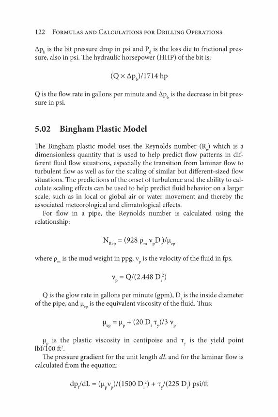
122 Formulas and Calculations for Drilling Operations
Δpb is the bit pressure drop in psi and P
d is the loss die to frictional pres-
sure, also in psi. The hydraulic horsepower (HHP) of the bit is:
(Q Δpb)/1714 hp
Q is the flow rate in gallons per minute and Δpb is the decrease in bit pres-
sure in psi.
5.02 Bingham Plastic Model
The Bingham plastic model uses the Reynolds number (Re) which is a
dimensionless quantity that is used to help predict flow patterns in dif-ferent fluid flow situations, especially the transition from laminar flow to turbulent flow as well as for the scaling of similar but different-sized flow situations. The predictions of the onset of turbulence and the ability to cal-culate scaling effects can be used to help predict fluid behavior on a larger scale, such as in local or global air or water movement and thereby the associated meteorological and climatological effects.
For flow in a pipe, the Reynolds number is calculated using the relationship:
NRep
= (928 ρm
νpD
i)/μ
ep
where ρm
is the mud weight in ppg, νp is the velocity of the fluid in fps.
νp = Q/(2.448 D
i2)
Q is the glow rate in gallons per minute (gpm), Di is the inside diameter
of the pipe, and μep
is the equivalent viscosity of the fluid. Thus:
μep
= μp + (20 D
i τ
y)/3 ν
p
μp is the plastic viscosity in centipoise and τ
y is the yield point
lbf/100 ft2. The pressure gradient for the unit length dL and for the laminar flow is
calculated from the equation:
dpf/dL = (μ
pν
p)/(1500 D
i2) + τ
y/(225 D
i) psi/ft

Hydraulics 123
For flow in the annulus:
NRea
= [(757 ρm
νa)(D
2 D
p)]/μ
ep
μep
= μp + 5(D
2 D
p)τ
y/ν
a
where D2 is the annulus diameter in inches, D
p is the outside diameter of
the pipe in inches, and νa is the velocity of the fluid in fps:
νa = Q/[2.448(D
22 D
p2) ft/sec
Thus, the pressure gradient for laminar flow is calculated from:
(dpf/dL) = (μ
pν
a)/[1000(D
2 D
p)2 + τy/[200(D
2 D
p)] psi/ft
Example calculationCalculate the change in the bottomhole pressure when the yield value is 5 lb/100 ft2 and the viscosity is 30 cp. Use the following data:
Hole size = 97⁄8 inchesDepth = 10,000 ftPipe OD = 4 inchesFlow rate = 400 gpmMud weight = 12 ppgYield point = 60 lb/100 ft2
Plastic viscosity = 40 cp
Solution:The annular velocity of the fluid is:
νa = 400/[2.448(9.8752 4.52)] = 2.11 ft/sec
The equivalent viscosity is:
μep
= 40 + [5 60(9.875 4.50]/2.11 = 802.5 cP
The Reynolds number is:
NRea
= [7.57 12 2.11(9.875 4.5)]/802.5 = 128
Since the Reynolds’s number is less than 2100, the flow is laminar.

124 Formulas and Calculations for Drilling Operations
The equivalent viscosity with new YP and PV is:
μep
= 5 + [5 30(9.875 4.5)]/2.11 = 93.5 cP and the Reynolds number (1104) is still indicating laminar flow. Thus:
dpf/dL = [(40 5)ν
a]/[1000(9.875 4.5)
2] + (60 30)/[200(9.875
4.5)] = 0.051985 psi/ft
Thus, the total pressure change is 0.051985 10,000 = 519 psi
5.03 Bit Hydraulics
5.03.1 Common Calculations
The total nozzle flow is calculated from the equation:
An = (π S
n2)/64 square inches
The nozzle velocity is:
Vn = 0.3208(Q/A
n) ft/sec
The pressure drop across bit is calculated from:
Δpb = (8.311 10−5 ρ
m Q2)/(C
d2 A
n2) psi
Cd is the discharge coefficient (usually a value of 0.95 is used). If the
value 0.95 is used, the pressure drop across the bit is:
Δpb = (ρ
m Q2)/(10858 A
n2) psi
Using nozzle velocity, the pressure drop across the bit is calculated from:
Δpb = (ρ
m V
n2)/1120 psi
The percentage pressure drop across the bit is:
Δpb/p
b 100

Hydraulics 125
The bit hydraulic power (BHHP) is calculated from:
HPb = (Q Δp
b)/1714
Hydraulic bit (jet) impact force (Fimp
) is calculated from:
Fimp
= 0.01823 Cd Q(ρ
m Δp
b)1/2 lbf
The hydraulic bit (jet) impact force (Fimp
) can also be written as:
Fimp
= [Q (ρm
Δpb)1/2]/57.66 lbf
The hydraulic bit (jet) impact force (Fimp
) with nozzle velocity can be written as:
Fimp
= (ρm
Q Vm
)/1930 lbf
The impact force per square inch of the bit area is calculated from:
Fimp
/[(π Db
2)/4] lbf in2
The impact force per square inch of the hole area is:
Fimp
/[(π Dh
2)/4] lbf in2
5.03.2 Optimization Calculations
The flow index is:
m = [log (Δpd)
j/(Δp
d)
i]/9log Q
j/Q
i)
For maximum bit hydraulic power:
Δpbopt
= [m/(m + 1)] Δpmax
The optimum flow rate is calculated from:
Qopt
= Qaalog[1/m log(Δp
dopt/Δp
dQa)

126 Formulas and Calculations for Drilling Operations
5.03.2.1 Limitation 1 – Available Pump Horsepower
For maximum impact force, the optimum bit pressure drop is:
Δpbopt
= [(m + 1)/(m + 2)] Δpbopt
The optimum flow rate is:
Qopt
= [92 Δpmax
)/c(m + 2)]1/m
5.03.2.2 Limitation 2 – Surface Operating Pressure
For maximum impact force, the optimum bit pressure drop is:
Δpbopt
= m/(m + 2)]Δpmax
Example calculationEstimate the optimum nozzle size and optimum flow rate for the following conditions:
m = 1.66Maximum allowed operating pressure = 5440 psiFrictional pressure loss = 2334 psi for a flow rate of 300 gpmVolumetric efficiency of the pump = 80%Mud weight = 15.5 ppgMinimum flow rate required for hole cleaning = 265 gpm
Solution:Using limitation 2 (above):
Δpbopt
= m/(m + 2)]Δpmax
Δpbopt
= 2/(166 + 2) 5440 = 2992 psi
Δpbopt
= Δpmax
Δpdopt
Δpbopt
= 5440 2975 = 2465 psi

Hydraulics 127
5.04 Critical Transport Fluid Velocity
The critical transport fluid velocity (CTFV) is the minimum fluid flow velocity in a pipe or annular region required to prevent the formation of a stationary cuttings bed. The CTFV is calculated using the equation:
Vca
= Vcr
+ Vcs
Vca
is the critical transport average annular fluid velocity, Vcr
is the cut-tings rise velocity, and V
cs is the cuttings average slip velocity.
5.05 Equivalent Circulating Density
The equivalent circulating density (ECD) results from the addition of the equivalent mud weight, due to the annulus pressure losses (Δp
a), to the
original mud weight (ρm
). Thus:
ECD = ρm
+ Δpa/(0.052 L
tvd) ppg
Example calculationCalculate the equivalent mud weight at a depth of 10,000 ft (TVD) with an annulus back pressure of 500 psi. The mud density in the annulus is 10 ppg.
Solution
EMW = ρm
+ 500/(0.052 10,000) = 10.96 ppg
5.06 Equivalent Mud Weight
The pressure in the wellbore or formation can be expressed in terms of equivalent mud weight (EMW) whohc is a convenient way in which to compare the pressure at any depth. This:
EMW = Ph/(0.052 L
tvd) ppg
Ph is the pressure in psi, and Ltvd is the true vertical depth in feet. If the well is deviated, then:
EMW = Ph/(0.052 D
h cos α) ppg

128 Formulas and Calculations for Drilling Operations
Dh is the measured depth in feet and α is the deviation in degrees from
the vertical.
5.07 Gel Breaking Pressure
In the pipe, the gel breaking pressure (P) is calculated from the equation:
P = (τg L)/(300 D
i) psi
Di is the inside diameter of the pipe, τ
g is the gel strength (lbf/100 ft2)
and L is the length of the pipe in feet. In the annulus:
P = (τg L)/300(D
hD
p) psi
Dh is the diameter of the hole in inches and D
p is the outside diameter of
the pipe, also in inches.
Example calculationMud circulation has been stopped for sufficient time to develop a gel strength of 15 lbf/100ft2. If the pipe is not moved, calculate the pressure surge required to break the circulation.
Depth = 10,000 ftDrill pipe = 5 inches × 4.27 inchesDrill collar = 450 feet, 6.5 inches × 3 inchesHole diameter = 8.5 inches
Solution:The pressure (P) required to break circulation is
P = [(15 9550)/(300 4.27)] + [(15 450)/(300 3)] + [(15 9550)/300(8.5 5)] + [(15 450)/300(8.5 6.5)]
P = 1181.8 + 7.5 + 136.43 + 11.25 = 267 psi
5.08 Hole Cleaning – Cuttings Transport
Drill cuttings are the broken bits of solid material removed from a bore-hole. The cuttings are commonly examined to make a record (a well log or sometimes called a mud log) of the subsurface materials penetrated at

Hydraulics 129
various depths. The cuttings concentration for 45° with one tool is given by the equation:
Cc = 3.22(1 + N
Ta)−0.472 + 5703.6N
Re−0.776 + 69.3
Rop−0.051
(1450 < NRe
< 3700, 0 < NTa
< 5800, 19.7 < NRop
< 23)
The cuttings concentration for 90° with one tool is given by the equation:
Cc = 5.22 10−5N
Ta1.36 + 605.714N
Re−0.0124
+ 8.86e230.43NRop
−77.58 529.4
(1450 < NRe
< 3700, 0 < NTa
< 5800, 19.7 < NRop
< 23)
For the above case with no tools and with a 45° inclination:
Cc = 1.81(1 + N
Ta)−8.13 + 21.25 e177.57N
Re−24.63
+ 15.7 e3.54NRop
−0.03 487.57
(1450 < NRe
< 3700, 0 < NTa
< 5800, 19.7 < NRop
< 23)
The cuttings concentration for 90° with no tool is given by the equation:
Cc = –14.04 e−316(1 + N
Ta)36.33 + 284.96N
Re−0.073
+ 58.2 e30.9NRop
−12.46 140.88
(1450 < NRe
< 3700, 0 < NTa
< 5800, 19.7 < NRop
< 23)
In the above equations, NTa
is Taylor’s number:
NTa
= ωρD2/μeff
D is the diameter of the hole in inches, ω is the angular velocity of the tool in radians per second, ρ
m is the mud density in ppg, and μ
eff is the effec-
tive viscosity in centipoise.
NRe
is the Reynold number = (ρV2−nDn)/K8n−1
K is the consistency index, V is the velocity of the fluid, and n is the power law index.
NRop
is the ROP number (rate of penetration): NRop
= (ρD ROP)/μ
eff

131
6.01 API Casing and Liners – Weight, Dimensions, Capacity, and Displacement
Nominal
size
inches
Weight with
coupling
lb/ft
Outside
diameter
inches
Inside
diameter
inches
Capacity
bbl/ft
Capacity
ft/bbl
Displacement
bbl/100 ft
4-1/2 9.50 4.500 4.090 0.0162 61.54 0.342
4-1/2 10.50 4.500 4.052 0.0159 62.70 0.372
4-1/2 11.60 4.500 4.000 0.0155 64.34 0.413
4-1/2 13.50 4.500 3.920 0.0149 67.00 0.474
4-1/2 15.10 4.500 3.826 0.0142 70.33 0.545
5 11.50 5.000 4.560 0.0202 49.51 0.409
5 13.00 5.000 4.494 0.0196 50.97 0.467
5 15.00 5.000 4.408 0.0189 52.98 0.541
5 18.00 5.000 4.276 0.0178 56.30 0.652
6Tubular Mechanics
(Continued)
Formulas and Calculations for Drilling Operations, Second Edition.James G. Speight.
© 2018 Scrivener Publishing LLC. Published 2018 by John Wiley & Sons, Inc.
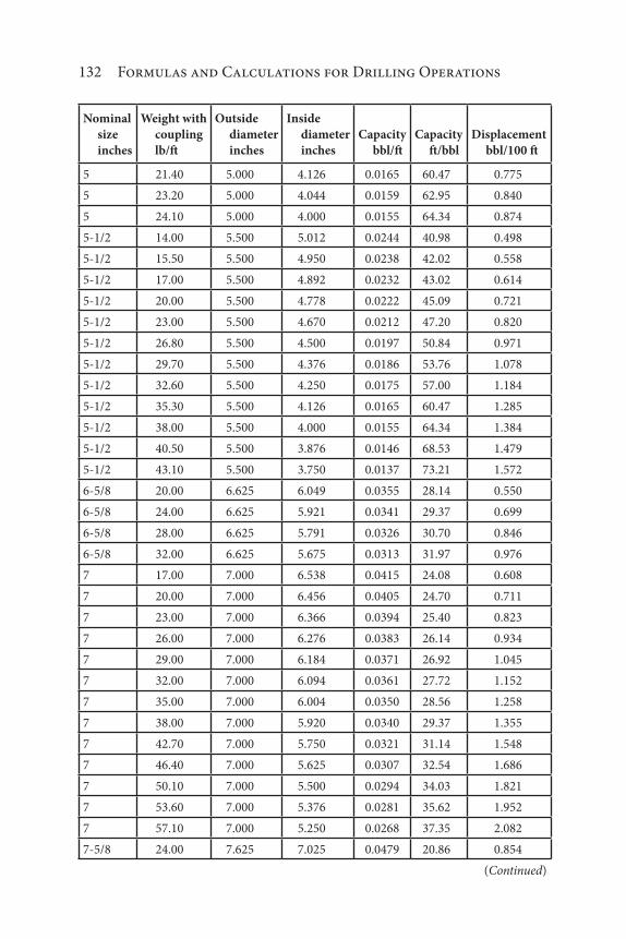
132 Formulas and Calculations for Drilling Operations
Nominal
size
inches
Weight with
coupling
lb/ft
Outside
diameter
inches
Inside
diameter
inches
Capacity
bbl/ft
Capacity
ft/bbl
Displacement
bbl/100 ft
5 21.40 5.000 4.126 0.0165 60.47 0.775
5 23.20 5.000 4.044 0.0159 62.95 0.840
5 24.10 5.000 4.000 0.0155 64.34 0.874
5-1/2 14.00 5.500 5.012 0.0244 40.98 0.498
5-1/2 15.50 5.500 4.950 0.0238 42.02 0.558
5-1/2 17.00 5.500 4.892 0.0232 43.02 0.614
5-1/2 20.00 5.500 4.778 0.0222 45.09 0.721
5-1/2 23.00 5.500 4.670 0.0212 47.20 0.820
5-1/2 26.80 5.500 4.500 0.0197 50.84 0.971
5-1/2 29.70 5.500 4.376 0.0186 53.76 1.078
5-1/2 32.60 5.500 4.250 0.0175 57.00 1.184
5-1/2 35.30 5.500 4.126 0.0165 60.47 1.285
5-1/2 38.00 5.500 4.000 0.0155 64.34 1.384
5-1/2 40.50 5.500 3.876 0.0146 68.53 1.479
5-1/2 43.10 5.500 3.750 0.0137 73.21 1.572
6-5/8 20.00 6.625 6.049 0.0355 28.14 0.550
6-5/8 24.00 6.625 5.921 0.0341 29.37 0.699
6-5/8 28.00 6.625 5.791 0.0326 30.70 0.846
6-5/8 32.00 6.625 5.675 0.0313 31.97 0.976
7 17.00 7.000 6.538 0.0415 24.08 0.608
7 20.00 7.000 6.456 0.0405 24.70 0.711
7 23.00 7.000 6.366 0.0394 25.40 0.823
7 26.00 7.000 6.276 0.0383 26.14 0.934
7 29.00 7.000 6.184 0.0371 26.92 1.045
7 32.00 7.000 6.094 0.0361 27.72 1.152
7 35.00 7.000 6.004 0.0350 28.56 1.258
7 38.00 7.000 5.920 0.0340 29.37 1.355
7 42.70 7.000 5.750 0.0321 31.14 1.548
7 46.40 7.000 5.625 0.0307 32.54 1.686
7 50.10 7.000 5.500 0.0294 34.03 1.821
7 53.60 7.000 5.376 0.0281 35.62 1.952
7 57.10 7.000 5.250 0.0268 37.35 2.082
7-5/8 24.00 7.625 7.025 0.0479 20.86 0.854
(Continued)

Tubular Mechanics 133
Nominal
size
inches
Weight with
coupling
lb/ft
Outside
diameter
inches
Inside
diameter
inches
Capacity
bbl/ft
Capacity
ft/bbl
Displacement
bbl/100 ft
7-5/8 26.40 7.625 6.969 0.0472 21.20 0.930
7-5/8 29.70 7.625 6.875 0.0459 21.78 1.056
7-5/8 33.70 7.625 6.765 0.0445 22.49 1.202
7-5/8 39.00 7.625 6.625 0.0426 23.46 1.384
7-5/8 42.80 7.625 6.501 0.0411 24.36 1.542
7-5/8 45.30 7.625 6.435 0.0402 24.86 1.625
7-5/8 47.10 7.625 6.375 0.0395 25.33 1.700
7-5/8 51.20 7.625 6.251 0.0380 26.35 1.852
7-5/8 55.30 7.625 6.125 0.0364 27.44 2.003
7-3/4 46.10 7.750 6.560 0.0418 23.92 1.467
8-5/8 24.00 8.625 8.097 0.0637 15.70 0.858
8-5/8 28.00 8.625 8.017 0.0624 16.02 0.983
8-5/8 32.00 8.625 7.921 0.0609 16.41 1.131
8-5/8 36.00 8.625 7.825 0.0595 16.81 1.278
8-5/8 40.00 8.625 7.725 0.0580 17.25 1.429
8-5/8 44.00 8.625 7.625 0.0565 17.71 1.578
8-5/8 49.00 8.625 7.511 0.0548 18.25 1.746
9-5/8 32.30 9.625 9.001 0.0787 12.71 1.129
9-5/8 36.00 9.625 8.921 0.0773 12.94 1.268
9-5/8 40.00 9.625 8.835 0.0758 13.19 1.417
9-5/8 43.50 9.625 8.755 0.0745 13.43 1.553
9-5/8 47.00 9.625 8.681 0.0732 13.66 1.679
9-5/8 53.50 9.625 8.535 0.0708 14.13 1.923
9-5/8 58.40 9.625 8.435 0.0691 14.47 2.088
9-5/8 59.40 9.625 8.407 0.0687 14.57 2.133
9-5/8 64.90 9.625 8.281 0.0666 15.01 2.338
9-5/8 70.30 9.625 8.157 0.0646 15.47 2.536
9-5/8 75.60 9.625 8.031 0.0626 15.96 2.734
10-3/4 32.75 10.750 10.192 0.1009 9.91 1.135
10-3/4 40.50 10.750 10.050 0.0981 10.19 1.414
10-3/4 45.50 10.750 9.950 0.0962 10.40 1.609
10-3/4 51.00 10.750 9.850 0.0942 10.61 1.801
(Continued)

134 Formulas and Calculations for Drilling Operations
Nominal
size
inches
Weight with
coupling
lb/ft
Outside
diameter
inches
Inside
diameter
inches
Capacity
bbl/ft
Capacity
ft/bbl
Displacement
bbl/100 ft
10-3/4 55.50 10.750 9.760 0.0925 10.81 1.972
10-3/4 60.70 10.750 9.660 0.0906 11.03 2.161
10-3/4 65.70 10.750 9.560 0.0888 11.26 2.348
10-3/4 73.20 10.750 9.406 0.0859 11.64 2.631
10-3/4 79.20 10.750 9.282 0.0837 11.95 2.856
10-3/4 85.30 10.750 9.156 0.0814 12.28 3.082
11-3/4 42.00 11.750 11.084 0.1193 8.38 1.477
11-3/4 47.00 11.750 11.000 0.1175 8.51 1.657
11-3/4 54.00 11.750 10.880 0.1150 8.70 1.912
11-3/4 60.00 11.750 10.772 0.1127 8.87 2.140
11-3/4 65.00 11.750 10.682 0.1108 9.02 2.327
11-3/4 71.00 11.750 10.586 0.1089 9.19 2.525
13-3/8 48.00 13.375 12.715 0.1570 6.37 1.673
13-3/8 54.50 13.375 12.615 0.1546 6.47 1.919
13-3/8 61.00 13.375 12.515 0.1521 6.57 2.163
13-3/8 68.00 13.375 12.415 0.1497 6.68 2.405
13-3/8 72.00 13.375 12.347 0.1481 6.75 2.568
16 65.00 16.000 15.250 0.2259 4.43 2.277
16 75.00 16.000 15.124 0.2222 4.50 2.648
16 84.00 16.000 15.010 0.2188 4.57 2.982
16 109.00 16.000 14.688 0.2096 4.77 3.911
18-5/8 87.50 18.625 17.755 0.3062 3.27 3.074
20 94.00 20.000 19.124 0.3553 2.81 3.329
20 106.50 20.000 19.000 0.3507 2.85 3.788
20 133.00 20.000 18.730 0.3408 2.93 4.778
6.02 API Drill Pipe Capacity and Displacement
Nominal
Size
inches
Weight
lb/ft
OD*
inches
ID**
Inches
Capacity
bbl/ft
Capacity
ft/bbl
Pipe
Displacement
bbl/100 ft
2-3/8 6.65 2.375 1.815 0.0032 311.43 0.228
2-7/8 10.40 2.875 2.151 0.0045 221.73 0.353
(Continued)

Tubular Mechanics 135
Nominal
Size
inches
Weight
lb/ft
OD*
inches
ID**
Inches
Capacity
bbl/ft
Capacity
ft/bbl
Pipe
Displacement
bbl/100 ft
3-1/2 9.50 3.500 2.992 0.0087 114.60 0.320
3-1/2 13.30 3.500 2.764 0.0074 134.29 0.448
3-1/2 15.50 3.500 2.602 0.0066 151.53 0.532
4 11.85 4.000 3.476 0.0118 84.91 0.381
4 14.00 4.000 3.340 0.0109 91.96 0.471
4-1/2 13.75 4.500 3.958 0.0153 65.49 0.445
4-1/2 16.60 4.500 3.826 0.0143 70.08 0.545
4-1/2 20.00 4.500 3.640 0.0129 77.43 0.680
5 16.25 5.000 4.408 0.0189 52.80 0.541
5 19.50 5.000 4.276 0.0178 56.11 0.652
5 25.60 5.000 4.000 0.0156 64.12 0.874
5-1/2 21.90 5.500 4.778 0.0223 44.94 0.721
5-1/2 24.70 5.500 4.670 0.0213 47.04 0.820
*OD: outside diameter
**ID: Inside diameter
6.03 Bending Stress Ratio
The bending stress ration (BSR) is the ratio of the box section modulus to the pin section modulus. Thus:
BSR = [(D4 b4)/D]/[Rt4 d4)/R
t]
D is the connection or tool outside diameter in inches, b is the thread root diameter of box threads at the end of the pin in inches, R
t is the thread root
diameter of pin threads 0.75 inches from the shoulder of the pin in inches, and d is the pin inside diameter in inches.
Typical accepted ranges of BSR are 2.25 to 2.75 for critical service appli-cation, 2.0 to 3.0 for normal service application, and 1.9 to 3.2 for limited service application.
6.04 Buckling Force
Buckling is instability in a structure that that leads to failure and occurs when a structure is subjected to compressive stress. Buckling is characterized by

136 Formulas and Calculations for Drilling Operations
a sudden sideways deflection of a structural member which may occur even though the stresses that develop in the structure are well below those needed to cause failure of the material of which the structure is composed.
The buckling force Fb is defined by the equation:
Fb = -F
a + P
iA
iP
oA
o
Fb is the buckling force, F
a is the axial force (tension positive), P
i is the
internal pressure, Ai is equal to πri2 where r
i is the inside radius of the tub-
ing, Po is the external pressure, and A
o is equal to πr
o2 where r
o is the outside
radius of the tubing. The Paslay buckling force, F
p, is defined by the equation:
Fp = [(4EIω
c)/r]1/2
Example calculationThe sample calculation given here is for determining the buckling of 2-7/8 inch, 6.5 lbm/ft tubing inside a 7 inch, 32 lbm/ft casing. The tubing is sub-merged in 10 lbm/gal packer fluid with no other pressures applied. Assume that an applied buckling force of 30,000 lbf is applied at the end of the string in a well with a 60° deviation from the vertical. The effect of the packer fluid is to reduce the tubing weight per unit length through buoyancy:
we = w + A
iρ
iA
oρ
o
where we is the effective weight per unit length of the tubing, Ai is the inside area of the tubing, ρi is the density of the fluid inside the tubing, Ao is the outside area of the tubing, and ρo is the density of the fluid outside the tubing. Thus:
we = 6.5 lbm/ft + (4.68 in2) (0.052 psi/ft/lbm/gal),
= (10.0 lbm/gal) (6.49 in2) (0.052 psi/ft/lbm/gal) (10.0 lbm/gal),
= 5.56 lbm/ft = 0.463 lbm/in.
6.05 Drag Force
In fluid dynamics, drag (also called air resistance, fluid resistance, or fluid friction) is the force acting opposite to the relative motion of any object

Tubular Mechanics 137
moving with respect to a surrounding fluid. This can exist between two fluid layers (or surfaces) or a fluid and a solid surface. Even though the ulti-mate cause of a drag is viscous friction, the turbulent drag is independent of viscosity. The drag force is proportional to the velocity for laminar flow and the squared velocity for turbulent flow.
Thus, drag force is given by the equation:
Fd = F
s μ (V
ts/V
rs)
Vts is the trip speed in inches per second, V
rs is the resultant speed in
inches per second, Fs is the side or normal force in lbs, and μ is the coef-
ficient of friction.
6.06 Drill Collar Length
The drill collar is a thick-walled tubular piece machined from a solid bar of steel, usually plain carbon steel but sometimes of nonmagnetic nickel-copper alloy or other nonmagnetic premium alloys. The drill collar size is defined by the equation:
Ddc
= (2Dcsg
Db)
Ddc
is the diameter of the drill collar, Dcsg
is the diameter of the casing coupling, and D
b is the diameter of the drill bit. Thus, the length of the drill
collar is given by:
Ldc
= (WOB DF)/(wdc
BF cos α)
WOB is the weight on the drill bit in lbs, DF is the design factor, wdc
is the unit weight of the collar in lbf/ft, BF is the buoyancy factor, and α is the wellbore inclination in degrees.
Example calculationAn 8½-inch, 22° hole is planned to be drilled and cased with 7-inch, 38 ppf, P-110 – BTC casing. The mud weight to be used is 12 ppg. The weight on bit desired is 25 kips. Calculate the size and length of drill collar required.
Solution:Coupling OD of the 7-inch” 38 ppf BTC is 7.656 inches. The diameter of the drill collar is:
Ddc
= 2 7.656 8.5 = 6.812 inches

138 Formulas and Calculations for Drilling Operations
The closest available drill collar sizes are 6¾ inches and 6½ inches. Typically, the 6½-inch drill collar is selected so that annular pressure losses against the drill collars, and thereby the equivalent circulating density, (ECD) are reduced.
6.07 Fatigue Ratio
The fatigue ratio (FRF, also called the endurance ratio) is the ratio of the
fatigue limit or fatigue strength to the static tensile strength of a material. Thus:
FRF = (σ
b + σ
buck)/σ
fl
In this equation, σb is the bending stress in psi, σ
buck = is the buckling
stress in psi, and σfl is the fatigue limit.
For tension, the fatigue limit can be written as:
σfl = σ
el(1 F
e/F
y)
where σel is the fatigue endurance limit of the pipe in psi, F
y is the yield
tension in lbf, and Fe is the effective tension in lbf. For compression, the
fatigue limit is:
σfl = σ
el
The axial force on the pipe has a remarkable impact on the fatigue fail-ure. The force required to generate the yield stress can be written as:
Fy = σ
ymin A
e
where σymin
is the minimum yield of the pipe in psi, and Ae is the effective cross-sectional area in square inches.
6.08 Length Change Calculations
Changing the mode of a well (producer, injector, shut-in, or treating) causes changes in temperature and pressure inside and outside the tubing. This, in turn, can create length and force changes in the tubing string that

Tubular Mechanics 139
can potentially affect the packer and downhole tools. The thermal induced stretch is calculated from the following equation:
ΔLt = La
t Δt
where at is the coefficient of thermal expansion which is the fractional
increase in length per unit rise in temperature, with units of in/in/F (with values of 6.9 × 10⁻⁶ for steel, 10.3 × 10⁻⁶ for aluminum, and 4.9 × 10⁻⁶ for titanium). Δt is the average temperature change in degrees Fahrenheit. If there is a linear variation of temperature along the wellbore, then:
ΔLt = α[Δt
o + (Δt/Δz)(L2/2)]
where z is the measured depth and Δ L is the measured calculation interval.
Example calculationCompute the elongation of 10,000 ft of 7-in casing due to temperature if the bottomhole temperature (BHT) is 290°F and the surface temperature is 70°F.
Solution
Δt = (final BHT + final surface temp)/2 (initial BHT + initial surface temp)/2
Δt = 110°F
ΔLt = 10,000 6.9 10−6 110 = 7.59 feet
6.09 Maximum Permissible Dogleg
Dogleg severity is a measure of the amount of change in the inclination, and/or azimuth of a borehole, usually expressed in degrees per 100 feet of course length. In the metric system, it is usually expressed in degrees per 30 meters or degrees per 10 meters of course length. The maximum per-missible dogleg and the axial stress are given by the equation:
σt = F
dls/A psi
A is the cross-sectional area of the drill pipe body in square inches and F
dls is the buoyed weight supported below the dogleg in lbs.

140 Formulas and Calculations for Drilling Operations
The maximum permissible bending stress for a drill pipe of grade E when the tensile stress is less than or equal to 67,000 psi is given by:
σb = 19,500 (10/67)σ
t (0.6/6702)(σ
t 33500)2
The maximum permissible bending stress for grade S drill pipe when the tensile stress is less than or equal to 133,400 psi is:
σb = 20,000[1 (σ
t/145,000) psi
The maximum possible dogleg severity is:
c = (432,000 σb)/πED
p (tan h KL)/KL
K = (T/EI)1/2
E = Young’s modulus in psi = 30 106 psi for steel and 10.5 106 psi for aluminum.
6.10 Pipe Wall Thickness and other Dimensions
6.11 Slip Crushing
Slip crushing refers to the maximum load that can be placed on the slips without damaging the specific tubular subjected to a tensile load. The cal-culation is dependent on the slip design, length of die contact to the pipe, the drill pipe thickness and yield strength. Thus, the maximum allowable load that can be supported by the slip is:
Fmax
= Fy/{[(2D
p2fA
p)/(D
p2 D
p2)A
s] + [(2D
p2fA
p)/(D
p2 D
i2)A
s)2]}1/2
Fy is the tensile strength of the pipe, lbf, A
s is the contact area between
slips and pipe (As = π D
pL
s ) in square inches, A
p is the cross sectional area
of the pipe in square inches, Dp is the outside diameter of pipe, in, D
i is the
inside diameter of pipe in inches, Ls is the length of slips, in, and f is the
lateral load factor of slips = (1- μ tan α)/(μ + tan α), where μ is the coef-ficient of friction between slips and bushings, and α is the slip taper angle in degrees.

Tubular Mechanics 141T
able
6.1
D
imen
sio
ns
for
Sch
edu
le 1
0, 4
0, 8
0 P
ipes
Pip
e si
ze*
O.D
. (in
.)
Sch
edu
le (
10
, 40
, 80
) w
all
thic
kn
ess
(in
ches
.)**
Sch
.10
Sch
.40
Sch
.80
Wal
l (i
n)
I.D
. (in
)W
all
(in
)I.
D. (
in)
Wal
l (i
n)
I.D
. (in
)
1/8
in
ch0
.41
od
0.0
49
in
0.3
12
id
0.0
7 i
n0
.26
9 i
d
Wei
ght
(lb
s/ft
.)St
eel
0.1
83
lb
s/ft
0.2
47
lb
s/ft
Stai
nle
ss
Alu
min
um
1/4
in
ch0
.54
od
0.0
65
in
0.4
10
id
0.0
90
in
0.3
64
id
0.1
19
in
0.3
02
id
Wei
ght
(lb
s/ft
.)St
eel
0.3
33
lb
s/ft
0.4
29
lb
s/ft
0.5
35
lb
s/ft
Stai
nle
ss
Alu
min
um
0
.14
7 l
bs/
ft
3/8
in
ch0
.67
5 o
d0
.06
5 i
n0
.54
5 i
d0
.09
1 i
n0
.49
3 i
d0
.12
6 i
n0
.42
3 i
d
Wei
ght
(lb
s/ft
.)St
eel
0.4
20
lb
s/ft
0.5
70
lb
s/ft
0.7
40
lb
s/ft
Stai
nle
ss
Alu
min
um
0
.19
6 l
bs/
ft
1/2
in
ch0
.84
0 o
d0
.08
3 i
n0
.67
4 i
d0
.10
9 i
n0
.62
2 i
d0
.14
7 i
n0
.54
6 i
d
Wei
ght
(lb
s/ft
.)St
eel
0.6
70
lb
s/ft
0.8
50
lb
s/ft
1.0
90
lb
s/ft
Stai
nle
ss
Alu
min
um
0
.29
4 l
bs/
ft0
.38
4 l
bs/
ft
(Con
tin
ued
)

142 Formulas and Calculations for Drilling OperationsT
able
6.1
C
on
t.
Pip
e si
ze*
O.D
. (in
.)
Sch
edu
le (
10
, 40
, 80
) w
all
thic
kn
ess
(in
ches
.)**
Sch
.10
Sch
.40
Sch
.80
Wal
l (i
n)
I.D
. (in
)W
all
(in
)I.
D. (
in)
Wal
l (i
n)
I.D
. (in
)
3/4
in
ch1
.05
0 o
d0
.08
3 i
n0
.88
4 i
d0
.11
3 i
n0
.82
4 i
d0
.15
4 i
n0
.74
2 i
d
Wei
ght
(lb
s/ft
.)St
eel
0.8
6 l
bs/
ft1
.13
lb
s/ft
1.4
8 l
bs/
ft
Stai
nle
ss
Alu
min
um
0
.39
10
.52
0
1 i
nch
1.3
15
od
0.1
09
in
1.0
97
id
0.1
33
in
1.0
49
id
0.1
79
in
0.9
57
id
Wei
ght
(lb
s/ft
.)St
eel
1.4
1 l
bs/
ft1
.68
lb
s/ft
2.1
7 l
bs/
ft
Stai
nle
ss
Alu
min
um
0.4
81
lb
s/ft
0.5
81
lb
s/ft
0.7
81
lb
s/ft
1-1
/4 i
nch
1.6
6 o
d0
.10
9 i
n1
.44
2 i
d0
.14
0 i
n1
.38
0 i
d0
.19
1 i
n1
.27
8 i
d
Wei
ght
(lb
s/ft
.)St
eel
1.8
1 l
bs/
ft2
.27
lb
s/ft
3.0
0 l
bs/
ft
Stai
nle
ss
Alu
min
um
0.6
18
lb
s/ft
0.7
85
lb
s/ft
1.0
40
lb
s/ft
1-1
/2 i
nch
1.9
0 o
d0
.10
9 i
n1
.68
2 i
d0
.14
5 i
n1
.61
0 i
d0
.20
0 i
n1
.50
0 i
d
Wei
ght
(lb
s/ft
.)St
eel
2.0
9 l
bs/
ft2
.72
lb
s/ft
3.6
3 l
bs/
ft
Stai
nle
ss
Alu
min
um
0.7
14
lb
s/ft
0.9
39
lb
s/ft
1.2
60
lb
s/ft

Tubular Mechanics 1432
in
ch2
.37
5 o
d0
.10
9 i
n2
.15
7 i
d0
.15
4 i
n2
.06
7 i
d0
.21
8 i
n1
.93
9 i
d
Wei
ght
(lb
s/ft
.)St
eel
2.6
4 l
bs/
ft3
.66
lb
s/ft
5.0
3 l
bs/
ft
Stai
nle
ss
Alu
min
um
0.9
03
lb
s/ft
1.2
60
lb
s/ft
1.7
40
lb
s/ft
2-1
/2 i
nch
2.8
75
od
0.1
20
in
2.6
35
id
0.2
03
in
2.4
69
id
0.2
76
in
2.3
23
id
Wei
ght
(lb
s/ft
.)St
eel
3.5
3 l
bs/
ft5
.80
lb
s/ft
7.6
7 l
bs/
ft
Stai
nle
ss
Alu
min
um
1.2
09
lb
s/ft
2.0
00
lb
s/ft
3 i
nch
3.5
0 o
d0
.12
0 i
n3
.26
id
0.2
16
in
3.0
68
id
0.3
0 i
n2
.90
id
Wei
ght
(lb
s/ft
.)St
eel
4.3
4 l
bs/
ft7
.58
lb
s/ft
10
.26
lb
s/ft
Stai
nle
ss
Alu
min
um
1.4
83
lb
s/ft
2.6
20
lb
s/ft
3.5
5 l
bs/
ft
3-1
/2 i
nch
4.0
0 o
d0
.12
0 i
n3
.76
id
0.2
26
in
3.5
50
id
0.3
18
in
3.3
60
id
Wei
ght
(lb
s/ft
.)St
eel
4.9
8 l
bs/
ft9
.12
lb
s/ft
12
.52
lb
s/ft
Stai
nle
ss
Alu
min
um
3
.15
0 l
bs/
ft4
.33
lb
s/ft
4 i
nch
4.5
0 o
d0
.12
0 i
n4
.26
id
0.2
37
in
4.0
26
id
0.3
37
in
3.8
26
id
Wei
ght
(lb
s/ft
.)St
eel
5.6
2 l
bs/
ft1
0.8
0 l
bs/
ft1
5.0
0 l
bs/
ft
Stai
nle
ss
Alu
min
um
1.9
22
lb
s/ft
3.7
30
lb
s/ft
5.1
80
lb
s/ft
(Con
tin
ued
)

144 Formulas and Calculations for Drilling OperationsT
able
6.1
C
ont.
Pip
e si
ze*
O.D
. (in
.)
Sch
edu
le (
10
, 40
, 80
) w
all
thic
kn
ess
(in
ches
.)**
Sch
.10
Sch
.40
Sch
.80
Wal
l (i
n)
I.D
. (in
)W
all
(in
)I.
D. (
in)
Wal
l (i
n)
I.D
. (in
)
5 i
nch
5.5
63
od
0.1
34
in
5.2
95
id
0.2
58
in
5.0
47
id
0.3
75
in
4.8
13
id
Wei
ght
(lb
s/ft
.)St
eel
7.7
8 l
bs/
ft1
4.6
3 l
bs/
ft2
0.8
0 l
bs/
ft
Stai
nle
ss
Alu
min
um
2.6
60
lb
s/ft
5.0
50
lb
s/ft
7.1
90
lb
s/ft
6 i
nch
6.6
25
od
0.1
34
in
6.3
57
id
0.2
80
in
6.0
65
id
0.4
32
in
5.7
61
id
Wei
ght
(lb
s/ft
.)St
eel
9.3
0 l
bs/
ft1
8.9
9 l
bs/
ft2
8.6
0 l
bs/
ft
Stai
nle
ss
Alu
min
um
3.1
81
lb
s/ft
6.5
60
lb
s/ft
9.8
80
lb
s/ft
8 i
nch
8.6
25
od
0.1
48
in
8.3
29
id
0.3
22
in
7.9
81
id
0.5
00
in
7.6
25
id
Wei
ght
(lb
s/ft
.)St
eel
13
.41
lb
s/ft
28
.58
lb
s/ft
43
.43
lb
s/ft
Stai
nle
ss
Alu
min
um
9
.88
lb
s/ft
15
.01
0 l
bs/
ft
*No
min
al s
izes
ap
ply
Pip
e Si
ze i
s th
e ge
ner
ic I
nd
ust
ry S
ize
Stan
dar
d f
or
refe
ren
ce o
nly
.
**T
ole
ran
ces
may
var
y sl
igh
tly
fro
m e
ach
man
ufa
ctu
rer

Tubular Mechanics 145
6.12 Stress
6.12.1 Radial Stress
The radial stress for a thick-walled pipe is given by the equation:
σr = [(p
ir
i2 p
or
o2)/(r
o2 r
i2)] + [r
i2r
o2(p
o p
i)/r2(r
o2 r
i2)]
In this equation, ri is the inner radius, r
o is the outer radius, p
i is the
inner absolute pressure and po is the outer absolute pressure.
6.12.2 Tangential Stress
Tangential stress (also called hoop stress or circumferential stress) is the force exerted circumferentially (perpendicular both to the axis and to the radius of the object) in both directions on every particle in the cylinder wall. It can be described as:
α = F/tl
F is the force exerted circumferentially on an area of the cylinder wall that has the following two lengths as sides: (i) t is the radial thickness of the cylinder and (ii) l is the axial length of the cylinder.
6.12.3 Longitudinal Stress
Longitudinal stress, also referred to as axial stress, can be calculated using the equation:
σa = F
T/[π(r
o2 r
i2) + σ
buck + σ
b
Example calculationCalculate the axial stress of the pipe with the following data:
True axial force = 64.6 kipsEffective force = 97.9 kipsPipe body diameter = 5 inchesPipe inside diameter = 4 inchesPipe data: premium class; assume no buckling and bending occurE = modulus of elasticity, psi; for steel = 30 × 106 psi

146 Formulas and Calculations for Drilling Operations
Solution:Derating the pipe based on the premium class,
Dcp
= c Dp + D
i(1-c)
New OD = 0.800 5.0 + 4.00(1.0 0.800) = 4.8 inches
The longitudinal stress inside the pipe is:
Σa = FT/π(ro
2 ri2) = 646000/π[(4.8/2)2 (4/2)2] = 11,683 psi
6.12.4 Stress Ratio
The stress ration is calculated from the equation:
X = (σy % yield)/σ
vm
where σy is the yield strength of the pipe in psi, and % yield is a percentage
used to reduce the yield strength of the pipe as a factor of additional safety. When X is equal to or less than 1, there is concern of failure.
6.13 Tension
Tension (the opposite of compression) is the pulling force transmitted axially by means of a string, cable, chain, or similar one-dimensional continuous object, or by each end of a rod, truss member, or similar three-dimensional object. Effective tension is given by the relationship:
Fe = F
i + F
bs
Fe = Fi + P
oA
o + P
iA
i
6.14 Torque
Torque is rotational force and is defined as the cross product of the vector by which the force’s application point is offset relative to the fixed suspen-sion point (distance vector) and the force vector, which tends to produce rotational motion. The magnitude of torque depends on three quantities: (i) the force applied, (ii) the length of the lever arm connecting the axis to

Tubular Mechanics 147
the point of force application, and (iii) the angle between the force vector and the lever arm. Thus:
τ = r F
In the equation, r is the position vector (a vector from the origin of the coordinate system defined to the point where the force is applied) and F is the force vector. The magnitude τ of the torque is given by the equation:
τ = r.F sin θ
In this second equation, r is the distance from the axis of rotation to the particle, F is the magnitude of the force applied, and θ is the angle between the position and force vectors.

149
7.01 Backoff Calculations
The force at the backoff depth id equal to the axial force down to well depth minus the axial force down to backoff depth. Thus, the surface axial force when the workstring is at a measured depth (MD) is:
ΣMD × (weight gradient + drag force gradient)
The rotary table torque at surface is equal to the torque at backoff depth plus the backoff torque.
Example calculationEstimate the surface action to backoff the string at a depth 9,000 ft with a backoff force and torque of 5 kips and 7,000 ft-lbf, respectively, applied at
7Drilling Tools
Formulas and Calculations for Drilling Operations, Second Edition.James G. Speight.
© 2018 Scrivener Publishing LLC. Published 2018 by John Wiley & Sons, Inc.

150 Formulas and Calculations for Drilling Operations
the backoff point. The string got stuck at 9,000 ft while tripping out. Other well and string details are given below:
Well depth = 10,000 ftWellbore details: casing with an inside diameter of 10” set at 6,000 ft and an open hole of 10-inch” diameterDrill string details:
Section type Length (ft) OD (in) ID (in) Weight (ppf)
Drill Pipe 7989 5 4 29
Drill Collar 540 8 2.5 154.3
Jar 30 8 3 147
Drill Collar 1440 8 2.5 154.3
Bit 1 10 95.37
Drill pipe tool joint details: 7.25” OD × 3.5” IDMud weight = 10.5 ppgAssume a friction factor of 0.3.The well is inclined 5° from the surface without any azimuth change.
Solution:Buoyed weight calculation:
For the drill pipe, assume the tool joint length is 5% of the string length.For the drill pipe, assume that the tool joint is 5% of the string length.
Thus:
Ao = π/490.95 D
p2 + 0.05 D
jt2)
= π/4(0.95 52 + 0.05 7.252)/144
= 0.14387 ft2
Ai = π/4(0.95 ID
p2 + 0.05 ID
jt2)
= π/4(0.95 42 + 0.05 3.52)/144 = 0.0862 ft2
wb = w
s +p
iA
ip
oA
o
= 29 + 7.48052 10.5(0.0862 0.14387)
= 24.4737 ppf

Drilling Tools 151
Similarly, Similarly, the buoyed weight for the drill collar and jar are 129.56 ppf and 123.4381 ppf, respectively.
Side force calculation:For the drill pipe, the side force of DP against the wellbore is equal to the component of the buoyed weight normal to the wellbore. Thus:
Fs = w
b sin α = 24.4737 × sin 5° = 2.133 ppf
Similarly, the side force against the drill collar and jar are 11.29 ppf and 10.76 ppf, respectively.
Drag force calculation:For the drill pipe, the drag force gradient is equal to the side force mul-tiplied by the friction factor (coefficient of friction). Thus, the drag force gradient of DP against the wellbore is given by the relationship:
Fd = F
s μ = 2.133 × 0.3 = 0.64 ppf
Similarly, the drag force gradient against the drill collar and jar are 3.39 ppf and 3.23 ppf, respectively.
Axial force at the backoff depth based on the trip out condition:Force at the backoff depth is equal to the axial force down to the well depth minus the axial force down to the backoff depth.
Surface axial force down to the well depth is:
ΣMD (Weight Gradient + Drag Force Gradient).
Thus:
7989(24.47 + 0.64) + 540(11.29 + 3.39) + 30(10.76 + 3.23) + 1440(11.29 + 3.39) = 230089.9 lbf
Measured weight at well depth = 230,0090 + 50,000 = 280,090 lbf = 280 kips.The axial force down to backoff depth:
= 7989(24.47 + 0.64) + 540(11.29 + 3.39) + 30(10.76 + 3.23) + 441(11.29 + 3.39) = 215425 lbf.

152 Formulas and Calculations for Drilling Operations
Final surface axial force for backoff operation:Measured weight at the surface for backing off is equal to the = axial force at backoff depth + backoff force + hoisting weight:
= 215425 + 5,000 + 50,000 = 270,424/1000 lbf = 270 kips.
The rotary table torque at the surface is equal to the torque at the backoff depth plus the backoff torque and the torque is equal to the component side force multiplied by the friction factor multiplied by the radius of the component.
The string torque at the backoff depth is:
7989[2.133 0.3 7.25/(2 12)] + 540[11.29 0.3 (8/(2 12)] + 30[1076 0.3(7.25/(2 12] + 441[11.29 0.3 8/(2 12)] = 2681
The surface torque for backoff = 2,681 + 7,000 = 9,681 ft-lbf.
7.02 Downhole Turbine
The torque developed is calculated from the relationship:
T = 2πQρm
r2nsNη
Q is the flow rate in gpm, ρm
is the mud weight in ppg, r2 is the square of the mean blade radius in square inches, ns is the number of turbine stages, N is the rotation speed of the turbine in rpm, and η is the efficiency.
Example calcualtionCalculate the torque developed by a hydraulic turbine with a flow rate of 400 gpm and 10 ppg mud.
Mean blade radius = 2.05 inchesNumber of stages = 100Rotation speed of turbine = 100 rpmOverall efficiency = 65%
Solution:The torque developed is calculated as
T = 2πQρm
r2nsNη

Drilling Tools 153
Thus:
T = 2π 400 10 2.052 100 100 0.65 ft lb
7.03 Jar Calculations
A jar is an impact tool installed in the drillstring to free stuck pipe. A jar concentrates kinetic energy at the point where the pipe is stuck.
7.03.1 Force Calculations for Up Jars
The effective jar set (cock) force is given by the relationship:
Fes = (Fs + Fpof
)
Fs is the set force, and F
pof is the pump open force.
The effective jar trip force is given by
Fet = (F
ts F
pof)
Fts is the trip force. An Induced force is required to set the jar at the cen-
ter of the jar in compression, and this requires over pulling the measured weight (hoisting/trip out). The set measured weight is given by:
Femw
= (Fti
Fs
Fpof
)
Ftis
is the trip in axial force, and Fs is the up jar set force.
An induced force is also required to trip the jar at the center of the jar in tension, and this requires slacking off the measured weight (lowering/trip in). The trip measured weight is given by the relationship:
Ftmw
= (Fto
+ Ft
Fpof
)
Fto
is the trip out axial force, and Ft is the up-jar trip force.
7.03.2 Force Calculations for Down Jars
The effective jar set (cock) force is calculated from the relationship:
Fes
= (Fs F
pof)

154 Formulas and Calculations for Drilling Operations
The effective jar trip force is calculated from:
Fes
= (Fts
Fpof
)
An induced force is required to set the jar at the center of the jar in tension, and this requires over pulling the measured weight (hoisting/trip out). The set measured weight is given by the equation:
Femw
= (Fto
+ Fs
Fpof
)
An induced force is required to set the jar at the center of the jar in tension, and this requires over pulling the measured weight (hoisting/trip out). Set measured weight is given by the relationship:
Ftmw
= (Fi
Ft
Fpof
)
Example calculationCalculate the jar forces using the following data:
Well depth = 8,000 ftDrill pipe = 7000 ft 5 inches, 4 inches OD, ID = 19.5 lb/ft (ppf), S = 105Drill collars = 500 ft, 8 inches OD, 3inches IDJar = 30 ft, 8 inches OD, 3 inches IDDrill collars = 500 ft, 8 inches OD, 3 inches IDBit = 12.25 inchesCasing = 5000 ft, 13.375 inchesOpen hole = 12.25 inchesHoisting equipment weight = 30 kipsTrip in axial force at the center of the jar = 150 kipsTrip out axial force at the center of the jar = 200 kipsPump open force = 3000 lbsType of jar: mechanicalUp jar set (cock) force = 40 kipsDown jar set (cock) force = 30 kipsMeasured weight when stuck = 350 kips
Solution:Up jar conditions:
Set (cock) measured weight at the surface = 150 40 3 + 30 = 137 kips.
Change in measured weight = 137 350 = -213 kips

Drilling Tools 155
The trip measured weight at the surface = 200 + 40 3 + 30 = 267 kips.
The change in set measured weight = 267 137 = 130 kips. Reset (re-cock) measured weight at the surface = 137 kips.The change in reset measured weight from the trip measured
weight = 137 267 = -130 kips.
Down jar conditions:Set (cock) measured weight at the surface = 200 +30 3 + 30
= 257 kips.Measured weight = 350 200 50 = 100 kips.Since the measured weight is less than the set measured weight,
the jar would have already set. For the down jar, for setting, the string must be tripped out to 257 kips, but the present measured weight in stuck conditions is 350 kips.
The change in measured weight = 350 350 = 0 kips.The trip measured weight at the surface = 150 40 3 + 30 =
137 kips.The change in set (cock) measured weight = 137 350 = 213
kips. Reset (re-cock) measured weight at the surface = 200 + 30 3 + 50 = 277 kips.
The change in reset measured weight from the trip measured weight = 277 137 = 140 kips.
7.04 Overpull/Slack-off Calculations
When the pipe is s tuck, if the surface measured weight at the stuck condi-tion is known, then
Fsp
= Ftd
Fsd
Fsp
is the force at stuck point depth, Ftd
is the axial force down to well depth, and F
sd is the axial force down to stuck depth.
When the pipe is stuck, if the surface measured weight at the stuck con-dition is known, then
F F Fsp td sd , (7.4)
where Fsp
= force at stuck point depth, Ftd
= axial force down to well depth, and F
sd = axial force down to stuck depth.

156 Formulas and Calculations for Drilling Operations
Problem 7.3Estimate the surface action to load the stuck point depth of 9,100 ft.
Use the data from Problem 7.2.
Solution:Axial force at the stuck point depth based on the trip out condition:
Force at stuck point depth = axial force down to well depth axial force down to backoff depth
The axial force down to well depth is
Ftd 7989 28 48 0 64 540 11 29 3 39 30 10 76 3 23
1440 11
. . . . . .
.. .
,
29 3 39
230 089 lbf.
The axial force down to the stuck points
7989(24.47 + 0.64) + 540(11.29 + 3.39) + 30(10.76 + 3.23) + 540(11.29 + 3.39) = 216,878 lbf.
The force at the stuck point depth
230 089 216 878 13 212 13 2, , , . lbf kips.
Measured weight
= 338,790 + 50,000 = 388,790 lbf = 389 kips.
The axial force at the stuck point depth based on the trip in condition is calculated as
Ftd
= 7989(24.47 0.64) + 540(11.29 3.39) + 30 (10.76 3.23) + 1540(11.29 3.39) = 207,035 lbf.

Drilling Tools 157
7.05 Percussion Hammer
For the percussion hammer, the work done (WD) is calculated by the equation:
WD = (Δpm
Ap L nb)/396,000 hp
In this equation, pm
is the pressure drop across the piston chamber in psi, A
p is the cross-sectional area of the piston in square inches, L is the
stroke length in inches, and nb is the number of blows of the piston per
minute.
Example calculationCalculate the work done in HP by a percussion hammer with the following details:
Pressure drop in the chamber = 400 psiDiameter of the pressure changer = 4 inchesStroke length = 1 footNumber of blows per minute = 200
WD = (400 π/4 12 200)/396,000 = 30.46 hp
7.06 Positive Displacement Motor (PDM)
The mechanical developed by the positive displacement motor (MHP) is given by the relationship:
MHP = [(T/550)/(2π/60)] N
N is the rpm.
7.07 Rotor Nozzle Sizing
The following simple steps help to size the nozzle effectively:
1. Establish the differential pressure range based on the expected weight on the bit range.

158 Formulas and Calculations for Drilling Operations
2. Calculate the range of operating flow rates, Qop, required for the run.
3. Estimate the minimum flow rate required for hole- cleaning, Qmin.
4. If the operating flow rate is less than the minimum flow rate for hole-cleaning, calculate the additional flow rate, Qrn, that will be bypassed through the rotor nozzle.
5. Size the nozzle using the equation:
Arn
= (8.311 10−5 Qrn
2 ρm
)/(Cd
2 Δpm
)
Arn
is the area of the rotor nozzle in square inches, Qrn
is the bypass flow rate through the rotor nozzle in gpm, ρ
m is mud
density of the circulating fluid in ppg, Cd is the discharge
coefficient, Δpm is the pressure drop across the motor in psi. The proper nozzle size can be calculated by rearranging the above equation. The rotor nozzle is often expressed in 32nds of an inch. If the rotor nozzle is specified as “14,” then the rotor nozzle has a diameter of 14⁄32 of an inch.
6. Check that the diameter of the nozzle is sufficiently smaller than the shaft diameter.
Example calculationA well is planned to be drilled with an 8.5-in class 1-1-1 bit, while the torque and rpm expected are 3000 ft-lbf and 300 rpm, respectively. The mud weight required is 10 ppg. Determine the size of the rotor nozzle for the following conditions:
Minimum flow rate required for hole-cleaning = 475 gpm
Configuration: 2/3Diameter of the motor = 6.75 inchesPitch of the housing = 23 inches
Solution:Diameter of the housing is assumed to be 6 inches. Thus, the pressure drop to be expected across the motor power section is:
Δpm
= 3000/[0.01 0.66(1.66/2-0.66632 23 26 0.7)]
= 836 psi

Drilling Tools 159
The operating flow rate requited is:
Qop
= (300 0.79 0.666 1.666 23 36)/(230.98 1.3332) = 530 gpm
Since this flow rate is higher than the minimum required flow rate of 475 gpm, there is no necessity to fit a rotor nozzle.
7.08 Stretch Calculations
Based on the pipe stretch under the applied tension, the approximate depth of the stuck point can be derived using the equation:
L = (E e W)/(144 ΔT ρs)
E is Young’s modulus in psi, e is the measured elongation corresponding to the differential tension (pull) in inches, W is air weight of the pipe in lb, ΔT is the differential pull or hook load in inches, and ρ
s is the density of
steel in lb/in3. For steel, the above equation can be written as:
L = (735294 e W)/ΔT
Example calculationA driller is planning to estimate the approximate stuck point in a vertical well by conducting the stretch test. The following is the observed data:
Initial pull = 210 kipsFinal pull = 240 kipsHook loads are greater than the weight of the string.Stretch of the pipe observed between these hook loads is found to be 19 inches.Drill pipe: 5 inches, 19.5 ppf, IEU
Calculate the estimated depth of the stuck point. Using the above equation, the depth of the stuck point is derived from
the equation above. Thus:
L = (735294 19 19.5)/(30 1,000) = 9,080 feet

161
8.01 Formation Pressure
Formation pressure arises from the pressure of fluids within the pores of a reservoir, usually hydrostatic pressure, or the pressure exerted by a col-umn of water from the formation’s depth to sea level. When a formation is impermeable, such as is the case in a shale formation, the pore fluids cannot always escape and must then support the total overlying sediments which leads to high formation pressures. Because reservoir pressure changes as fluids are produced from a reservoir, the pressure should be described as measured at a specific time, such as initial reservoir pressure.
8.01.1 Hubert and Willis Correlation
The matrix stress is calculated from the relationship:
σz = σ ob pp psi
8Pore Pressure and Fracture Gradient
Formulas and Calculations for Drilling Operations, Second Edition.James G. Speight.
© 2018 Scrivener Publishing LLC. Published 2018 by John Wiley & Sons, Inc.

162 Formulas and Calculations for Drilling Operations
In this equation, where σob is the overburden pressure in psi, and pp is the pore pressure, also psi.
The fracture pressure is obtained from the relationship:
pff = σ
h + p
p psi
pff = σ
min + p
p psi
σh is the horizontal stress in psi and σ
min is the minimum horizontal
stress, also in psi. The Horizontal stress is assumed to be one-half and one-third of the overall stress. Thus:
σhmin
= 0.33σz = 0.33(σ
obp
p) psi
σhmax
= 0.5σz = 0.5(σ
obp
p) psi
Thus, the fracture pressure is calculated from the relationship:
pff = 0.33σ
z = 0.33(σ
obp
p) psi
pff = 0.5σ
z = 0.5(σ
obp
p) psi
In terms of pressure gradient:
pffmin
/D = 0.33[(σob
pp)/D] psi
pff/D = 0.5[(σ
obp
p)/D] psi
D is the depth in feet.
8.01.2 Matthews and Kelly Correlation
The minimum pressure required to create a fracture is at least the forma-tion fluid pressure, and any additional pressure may be related to overcome the formation matrix:
σz = σ
obp
p psi
σmin
= Fsσ
z psi
pff = F
σσ
z + p
p psi
pff/D = (F
σσz)/D + p
p/D psi/ft
Fσ is the matrix coefficient

Pore Pressure and Fracture Gradient 163
8.01.3 Eaton’s Correlation
The horizontal and vertical stress ratio and the matrix stress coefficient are dependent on the Poisson’s ratio of the formation.
σx + σ
y + σ
h = [μ/(1 μ)]σ
z psi
pff = [μ/(1 μ)](σ
obp
p) + p
p psi
pff/D = [μ/(1 μ)][(σ
obp
p)/D] + p
p/D psi/ft
In these equations, μ is the Poisson ratio.
8.01.4 Christman’s Correlation
The effect of the water depth in calculating the overburden gradient is accounted for by the relationship:
pff/D = (1/D)(ρ
wD
w + ρ
bD
f) psi/ft
If it is assumed that the density of sea water is 1.02 gm/cc, the equation becomes:
pff/D = (1/D)(0.44D
w + ρ
bD
f) psi/ft
8.02 Leak-off Pressure
Leak-off occurs when the fracture area is constant during shut-in and the leak-off occurs through a homogeneous rock matrix. The formation breakdown gradient is equal to the leak-off pressure minus the true vertical depth (TVD) of the shoe). Thus, the equivalent mud weight to fracture the formation is derived from the equation:
ρff = ρ
s/(0.052 D
v) + ρ
test ppg
ps is the surface leak-off pressure during the test in psi, Dv is the true vertical depth of the formation tested in feet, and ptest is the mud weight during the test in ppg. The maximum fracture pressure equivalent mud weight required to drill the next formation interval is derived from the equation: (p
ffp
test)0.052 D
v in ppg.

164 Formulas and Calculations for Drilling Operations
Example calculationCalculate the mud weight required to break down the formation with the following data taken during a leak-off test.
Surface pressure during the leak-off = 500 psiMud weight during the test = 10 ppgTrue vertical depth of the formation tested = 5002 feet
Solution:The equivalent leak-off mud weight
ρff = ρ
s/(0.052 D
v) + ρ
test ppg
= 500/(0.052 5002) + 10 = 11.922 ppg
The formation pressure at the leak-off depth derives using the equation is:
Pff = 0.052 11.922 5002 = 3,101 psi

165
9.01 Accumulators
In the drilling technology area, a hydraulic accumulator is a pressure stor-age reservoir in which a non-compressible hydraulic fluid is held under pressure that is applied by an external source. An accumulator enables a hydraulic system to cope with extremes of demand using a less powerful pump, to respond more quickly to a temporary demand, and to smooth out pulsations. Compressed gas accumulators, also called hydro-pneumatic accumulators, are by far the most common type of accumulators.
An accumulator follows a specific charging sequence. Thus: The volume delivered by the accumulator bottles is given by the formula:
Vd = (P
pc/P
f P
pc/P
s) V
b
Ppc
is the nitrogen pre-charge pressure in psi, P
f is the final operating
pressure of the bottle in psi, P
s is the accumulator system pressure in p
si, and
Vb is the actual bottle capacity in gallons.
9Well Control
Formulas and Calculations for Drilling Operations, Second Edition.James G. Speight.
© 2018 Scrivener Publishing LLC. Published 2018 by John Wiley & Sons, Inc.

166 Formulas and Calculations for Drilling Operations
For sub-sea operations, the volume delivered is given by the equation:
V = Vd[(460 + T2)(460 + T
1)]
where T1 is the ambient temperature in degrees Fahrenheit and T2 is tem-
perature at water depth, also in degrees Fahrenheit.
Example calculationCompute the total amount of fluid delivered from eight 20-gallon bottles with a system pressure of 3,000 psi. The pre-charge pressure is 1100 psi, and the final pressure is 1250 psi.
Solution:The volume delivered is calculated from the equation:
Vd = (P
pc/P
f P
pc/P
s) V
b = 8 [(1100/1250 1100/3000)] 20
= 81.6 gallons
9.02 Driller’s Method
Assuming a gas kick, during the first circulation the kick fluid is circulated out of annular space using the original light mud with- out allowing any further kick fluid intrusion by keeping the circulating drill pipe pressure at:
Pcdpi = Ppr + Psidp.
Figure 9.1 Charging Sequence for an Accumulator.
Fully charged
Usable fluid
Partially chargedPre chargedAtmospheric pressure

Well Control 167
Afterwards, close the choke and read Psidp and Psic and the two should be equal. If not, continue circulating until all gas is removed from the well.
During the second circulation, a volume of the heavy kill mud that is equal to the total drillstring volume capacity is circulated while keeping the choke pressure at Psidp. The circulating drill pipe pressure should drop from Pcdpi at the beginning of the circulation to Pcdpf when the new mud reaches the bit. Circulation of heavy mud is continued until all original mud in the annulus is displaced. Afterwards, close the choke and read Psidp and Psic and the two should be equal to 0 psi. If so, open the well and resume the drilling operations. If not, continue the well control operation.
9.03 Formulas Used in Kick and Kill Procedures
9.03.1 Hydrostatic Pressure (psi): MW TVD 0.0519 MW is the Mud Density (lb/gal) TVD is the True Vertical Depth (ft)9.03.2 Circulating Pressure (psi): (MW TVD 0.0519) + Pla Pl
a is the Annular Pressure Loss (psi)
9.03.3 Initial Circulating Pressure (psi): SPR + SIDP SPR is the System pressure loss at kill rate (psi) SIDP is the Shut-in Drill Pipe Pressure (psi)9.03.4 Final Circulating Pressure (psi): (KMW/MW) SPR KMW = Kill Mud Density (lb/gal)9.03.5 Kill Mud Weight (lb/gal): MW + (SIDP / (TVD 0.0519))9.03.6 Formation Pressure (psi): SIDP + (MW TVD 0.0519)9.03.7 Density of influx (ppg): MW [(SICP SIDP)/(L 0.0519)] SICP is the Shut-in casing pressure (psi) L is the Length of influx (ft)9.03.8 Length of kick around drill collars (ft): Pit Gain* (bbls)/Annular Volume around collars (bbls/ft)9.03.9 Length of kick, drill collars and drill pipe (ft): Collar Length + [(Pit Gain* Collar Annular Volume)/(D
12
D2
2 0.000971)] D
1 is the hole diameter (inches)
D2 is the drill pipe diameter (inches)
9.03.10 Gas bubble migration rate (psi/hr): ΔPa / (0.0519 MW) ΔPa is the pressure change over time interval/time interval (hr)9.03.11 Barite required (sk/100 bbls mud): 1490 (KMW MW) /
(35.8 KMW)

168 Formulas and Calculations for Drilling Operations
9.03.12 Volume increase caused by weighting up: 100 (KMW MW) / (35.8 KMW)
*Fluids entering the wellbore displace an equal volume of mud at the flow-line, resulting in pit gain.
9.04 Hydrostatic Pressure Due to the Gas Column
The surface pressure due to the gas column is given as
Pg = Poe(0.01877 ρg D)/ZT
Po is the formation pressure of gas in psi, ρg is the density of the gas in ppg, D is the height of the gas column in feet, T is the temperature in degrees Kelvin, Z is the compressibility factor at temperature T, and P Po the hydrostatic pressure in psi.
Example calculationA 10,000 ft well full of gas was closed at the surface. The formation pressure and temperature is 6,200 psi and 180°F, respectively. Assume a gas gravity of 0.7 and Z = 0.9 and a temperature equal to 180 + 460 = 640°K.
The surface pressure due to the gas column is given by the relationship:
Pg = Poe(0.01877 ρg D)/ZT = 6200e(0.0187 0.7 10000)/(0.9 630) = 7788.57 psi
The hydrostatic pressure exerted due to the gas column is:
Pg Po = 7788.57 6200 = 1589 psi
9.05 Kill Methods
The two widely used constant bottomhole circulating methods are the Driller’s Method and the Wait and Weight (W&W) Method. The basic prin-ciple of both methods is to keep bottomhole pressure (BHP) constant at or, preferably, slightly above the formation pressure. Relevant formulas are:
1. Kill Weight Mud
KWM = OMW + [SIDPP ÷ (0.052 TVD)]

Well Control 169
KWM is the kill weight mud in ppg, OMW is the original mud weight in ppg, SIDPP is shut in drill pipe pressure in psi, TVD is the true vertical depth of the well in feet.
2. Slow Circulating Rate (SCR)
SCR = ICP – SIDPP
SCR is the slow circulating rate in psi, ICP is the initial cir-culating pressure in psi, and SIDPP is the shut-in drill pipe pressure in psi.
3. Final Circulating Pressure (FCP)
FCP = SCR KWM ÷ OMW
FCP is the final circulating pressure in psi, SCR is the slow cir-culating rate in psi, and KWM is the kill weight mud in ppg.
9.06 Kill Mud Weight
The formation pressure is calculated from the relationship:
Pf = 0.062 ρ
m D
v + P
sidp psi
Thus, the kill mud weight, Km
, is:
Km
= ρm
+ [Psidp
/(0.052 Dv)] + ρ
ok psi
In this equation, ρm is the original mud weight in ppg, Psidp is the shut-in drill pipe pressure in psi, Dv is the vertical depth in feet, and ρok is the overkill safety margin in ppg.
The initial circulating pressure (ICP) is:
ICP = Psidp + Pp + Po
Psidp = the shut-in drill pipe pressure in psi, Pp is the slow circulating pump pressure in psi, and Po is the overkill pressure, psi. Thus, the final circulating pressure (FCP) is:
FCP = Pp (ρ
km/ρ
om)

170 Formulas and Calculations for Drilling Operations
Example calculationEstimate the kill fluid density for a shut-in-drill pipe pressure of 580 psi. The kick depth is 11,937 feet and the original mud density is 14.3 ppg.
Solution:
Kill fluid density = 14.3 + 580/(0.052 11937) = 15.3 ppg
Kill fluid gradient = 14.3 0.052 + 480/11937 = 0.7922 psi/foot.
9.07 Leak-off Pressure
Typically leak-off occurs when the fracture area is constant during shut-in and the leak-off occurs through a homogeneous rock matrix. The leak-off pressure, also often referred to as the formation breakdown pressure, is calculated from the relationship:
Pff = 0.052 D
v ρ
m + P
lop psi
Dv is the true vertical depth in feet, ρ
m is the mud density, and P
lop is the
surface leak-off pressure. The equivalent mud gradient is calculated using the relationship: P
ff/D
v
psi/foot and the formation breakdown gradient, FBG, is calculated as:
FBG = (Pff -D
v ρ
sw)/(D
v D
a D
s)
Dv is the true vertical depth in feet, ρ
sw is the sea water density in ppg, D
a
is the air gap in feet, and Ds is the sea depth in feet.
Example calculationA well planner calculates the equivalent fracture gradient using the follow-ing relationship:
ρff = [F
s(σ
ob0.052) ρ
f] + ρ
f
The overburden gradient, σob
, is 0.89934e0.0000Dv and the matrix stress ratio, F
s, is calculated as:
Fs = 0.327279+ 6.94721 10−5Dv 1.98884 10−9Dv
2
Calculate the formation gradient at a depth 9.875 ft.

Well Control 171
Solution:The matrix stress ratio at 9,875 ft is calculated from the equation:
Fs = 0.327279 + 6.94721 10−59875 1.98884 10−998752 = 0.823
The overburden gradient is:
σob
= 0.89934e0.0000x9875 = 0.9938 psi/foot
The formation fracture gradient is calculated as
ρff = 0.823(0.9938/0.052 9) + 9 = 17.32 ppg
9.08 Length and Density of the Kick
A kick is an undesirable influx of formation fluid into the borehole. If left unattended, a kick can develop into a blowout (an uncontrolled influx of formation fluid into the borehole). Failure to control a kick can be the loss of the well and serious consequences for the rig and the health and welfare of the crew.
9.08.1 Length of the Kick
Length of the kick, ft = pit gain, bbl/(annulus capacity behind drill collar, bbl/ft)
For pit gain, bbl < annulus volume against drill collar, bbl:
Length of the kick, ft = length of the drill collar, ft + (pit gain, bbl annulus volume against drill collar, bbl)/annulus capacity
behind drill pipe, bbl/ft
For pit gain, bbl > annulus volume against drill collar, bbl
9.08.2 Density of the Kick
Density of the kick, ppg = initial mud weight, ppg (initial stabilized drill pipe pressure in psi initial stabilized casing pressure, psi)/(0.052 Length of the kick, ft)

172 Formulas and Calculations for Drilling Operations
9.08.3 Type of Kick
A gas kick is given by: ρk < 0.25 psi/ft
An oil and gas mixture is given by: 0.25 < ρk < 0.3 psi/ft.
An oil or condensate is given by: 0.3 < ρk < 0.4 psi/ft
A water kick is given by: 0.4 < ρk psi/ft
9.08.4 Kick Classification
The kick while drilling is classified using the following criteria:
Pore pressure > dynamic bottomhole pressure > static bottomhole pressure
The kick after pump shutdown is classified by the following criteria:
Dynamic bottom hole pressure > pore pressure > static bottomhole pressure
The swab kick is classified by the following criteria:
Dynamic bottomhole pressure > static bottomhole pressure > sore pressure
Example calculationA kick was taken when drilling a high-pressure zone of a depth of 9,875 ft with a mud density of 9 ppg. After the well was shut-in, the pressures recorded were SIDP = 300 psi and SICP = 370 psi. The total pit gain observed was 5 bbl. The annular capacity against 900 ft of drill collar is 0.0292 bbl/ft. The overkill safety margin is 0.5 ppg. Calculate the formation pressure, kick density, the type of fluid, and the required kill mud weight.
Solution:The formation pressure, P
f, is calculated from the equation:
Pf = 0.052 ρ
m D
v + P
sidp = 0.052 9 9875 + 300 = 4921 psi
Total annular volume against the drill collar is equal to 0.0292 900 = 26.28 bbl. Therefore, the volume of the kick is
Vk < V
an/dc

Well Control 173
Therefore, the length of the kick is:
Lk = V
k/C
an/dc = 5/0.0292 = 171.23 ft
The density of the kick fluid is:
ρk = ρ
m = (P
sidp P
sicp)/(0.052 L
k) = 9 + (300 370)/0.052
171.23) = 1.13 ppg
Therefore, the kick fluid is gas. The kill mud weight is:
ρkm
= ρm
+ Psidp
/(0.052 Dv) + ρ
ok = 9 + 300/(0.052 9875
+ o.5 = 10.08 ppg)
9.08.5 Kick Tolerance
In terms of kick tolerance:
1. If Dv
Lk < D
cs, then:
KT = (ρ
ffρ
k)(D
cs/D
v) + ρ
k ρ ppg
2. If Dv
Lk > D
cs, then:
KT = (ρ
ffρ)(D
cs/D
v) + (ρ ρ
k)(L
k/D
v) ppg
where ρff is the formation fracture gradient at the shoe in
ppg, Dcs is the vertical depth of the shoe in feet, ρk is the den-
sity of the kick in ppg, ρ is the density of the wellbore mud at the time of the kick in ppg, and L
k is the length of the kick.
Example calculationDetermine the kick tolerance for the following data:
Well depth = 9,878 ftCasing shoe depth = 6,500 ftMud density = 10.1 ppgEquivalent fracture mud weight at the shoe = 14.8 ppgVolume of the kick = 10 bblAnnulus capacity of 1,080 ft of drill collar = 0.0292 bbl/ftKick density = 2 ppg

174 Formulas and Calculations for Drilling Operations
Solution:The total annular volume against the drill collar is 0.0292 × 1080 = 31.536 bbl.
Therefore, the volume of the kick is: Vk < V
an/dc
The length of the kick, Lk, is calculated is:
Lk = V
k/C
an/dc = 10/0.0292 = 342.46 feet
Calculating Dv
Lk = 9878 342.46 = 9535.53, which is > D
cs = 6500ft.
Therefore, using the second condition:
KT = (ρ
ffρ)(D
cs/D
v) + (ρ ρ
k)(L
k/D
v)
= 14.0 10.1(6500/9878) + (10.1 2)(342.46/9878) 3.37
9.09 Maximum Allowable Annular Surface Pressure
The maximum allowable annular surface pressure (MAASP) (static) is given by the equation:
Psmaasp
= 0.052(ρf
ρm
)/Dsv
psi
Dsv
is the shoe depth (TVD) in feet, ρf is the equivalent fracture mud
weight in ppg, and ρm
is the wellbore mud weight in ppg. The maximum allowable annular surface pressure (dynamic) is given by
the equation:
Pdmaasp
= 0.052(ρf
ρm
)/Dsv
Δpa
psi
Δpa
is the annular frictional pressure loss above the shoe in psi.
Example calculationA well is being drilled with a mud weight of 14 ppg at a depth of 15,000 ft (TVD) has a shoe at 13,100 ft (TVD). The fracture gradient at the shoe is 0.85 psi/ft. Calculate the maximum allowable annular surface pressure.
SolutionThis is a static condition. Therefore, the equivalent fracture mud weight, ρ
f, is:
ρf = 0.85/0.52 = 16.35 ppg

Well Control 175
The maximum allowable annular surface pressure (static) is:
Psmaasp
= 0.052(16.35 14)13100 = 1598psi
9.10 Riser Margin
Riser margin is equal to (drilling fluid gradient to control the formation pressure with riser in psi/foot multiplied by the depth of the hole (TVD) in feet minus the seawater gradient in psi/foot. The seawater gradient in psi/foot is the water depth in feet divided by the depth of the hole (TVD) in feet minus the water depth in feet. Thus, and equation by which the riser margin can be calculated is:
ρrm
= (ρemw
Dv ρ
wD
w)(D
vD
wD
a)
In this equation, ρemw
is the drilling fluid gradient to control the forma-tion pressure with the riser in psi/ft, D
v is the depth of the hole (TVD) in
feet, ρv is the seawater gradient, psi/ft, D
w is the water depth in feet, and D
a
is the air gap, feet.
Example calculationCalculate the riser margin for the given data: (i) water depth = 3575 ft, (ii) air gap = 75 ft, (iii) depth of the hole = 15,554 ft (TVD), and (iv) the forma-tion gradient at the depth of hole is 0.78 psi/ft.
Solution:The riser margin is:
(0.78 15554 0.434 3575)/(15554 3575 75) = 0.89psi/ft
The safety riser margin = 0.89 0.78 = 0.11 psi/ft

177
10Drilling Problems
10.01 Differential Sticking Force
Differential sticking – a problem that occurs worldwide in terms of time and financial cost – is a condition whereby the drill string cannot be moved (rotated or reciprocated) along the axis of the wellbore and typically occurs when high-contact forces caused by low reservoir pressure, high wellbore pressure, or both, are exerted over a sufficiently large area of the drillstring. Differential sticking is a product of the differential pressure between the wellbore and the reservoir and the area that the differential pressure is act-ing upon. This means that a relatively low differential pressure (Δp) applied over a large working area can be just as effective in sticking the pipe as can a high differential pressure applied over a small area.
The formula for the approximate calculation of the differential sticking force due to fluid filtration is:
Fpull
= μΔPAc
Formulas and Calculations for Drilling Operations, Second Edition.James G. Speight.
© 2018 Scrivener Publishing LLC. Published 2018 by John Wiley & Sons, Inc.
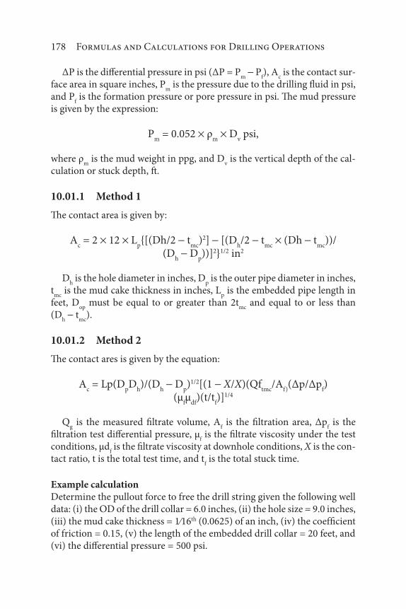
178 Formulas and Calculations for Drilling Operations
ΔP is the differential pressure in psi (ΔP = Pm
Pf), A
c is the contact sur-
face area in square inches, Pm
is the pressure due to the drilling fluid in psi, and P
f is the formation pressure or pore pressure in psi. The mud pressure
is given by the expression:
Pm
= 0.052 ρm
Dv psi,
where ρm
is the mud weight in ppg, and Dv is the vertical depth of the cal-
culation or stuck depth, ft.
10.01.1 Method 1
The contact area is given by:
Ac = 2 12 L
p{[(Dh/2 t
mc)2] [(D
h/2 t
mc (Dh t
mc))/
(Dh D
p))]2}1/2 in2
Dh is the hole diameter in inches, D
p is the outer pipe diameter in inches,
tmc
is the mud cake thickness in inches, Lp is the embedded pipe length in
feet, Dop
must be equal to or greater than 2tmc
and equal to or less than (D
h t
mc).
10.01.2 Method 2
The contact ares is given by the equation:
Ac = Lp(D
pD
h)/(D
h D
p)1/2[(1 X/X)(Qf
tmc/A
f)(Δp/Δp
f)
(μfμ
df)(t/t
f)]1/4
Qg is the measured filtrate volume, A
f is the filtration area, Δp
f is the
filtration test differential pressure, μf is the filtrate viscosity under the test
conditions, μdf is the filtrate viscosity at downhole conditions, X is the con-
tact ratio, t is the total test time, and tf is the total stuck time.
Example calculationDetermine the pullout force to free the drill string given the following well data: (i) the OD of the drill collar = 6.0 inches, (ii) the hole size = 9.0 inches, (iii) the mud cake thickness = 1⁄16th (0.0625) of an inch, (iv) the coefficient of friction = 0.15, (v) the length of the embedded drill collar = 20 feet, and (vi) the differential pressure = 500 psi.

Drilling Problems 179
Solution
μ = 0.15. ΔP = 500 psi. Lp = 20 ft.
Thus:
Ac = 2 20 12[(9/2 0.0625)2 (9/2 0.0625)(9 6)2]1.2
= 500.4 square inches
Therefore, pull out force = μΔPAc = 0.15 2.085 500 = 37,530 lbf
10.01.3 Method 3
The arc length at the contact point is derived using the equation:
Ac = (α/2)D
p L
p
sin α = [ε(X + ε)(X + Dp + ε)D
p ε)]1/2/[(X/2 + ε)D
p]
X is equal to Dh D
p 2t
mc, α is the angle of contact between the bot-
tom hole assembly (BHA) section and the mud cake in radians, and ε is the deformation of the mud cake at the mid-point of contact in inches.
10.02 Hole Cleaning–Slip Velocity Calculations
The slip velocity arises because of the difference between the average veloc-ities of two different fluids flowing together in a pipe. In vertical ascending flow, the lighter fluid flows faster than the heavier fluid. The slip velocity depends mainly on the difference in density between the two fluids, and their respective hold up.
10.02.1 Chien Correlation
The slip velocity if given for two conditions as illustrated in the following equations:
vs = 0.458β{[36800d
s/β
2)(ρ
s ρ
m/ρ
m)]1/2 + 1 1} (for β < 10)
vs = 86.4d
s(ρ
s ρ
m/ρ
m)]1/2 (for β > 10)

180 Formulas and Calculations for Drilling Operations
In these equations, β = μa/μ
mds and μ
a = μ
p + (300τ
yd
s/V
a) where ρm is the
mud density in ppg, ρs is the cuttings density in ppg, μ
a is the mud apparent
viscosity in centipoise, μp is the mud plastic viscosity in centipoise, τy is the
mud yield value lb/100 ft2, ds is the equivalent spherical diameter of cutting
in inches, and Va is the average annular fluid velocity (fpm).
Va = 60Q/(2.448(D
h2 D2) ft/min
Q is the flow rate in gpm, Dh is the inside diameter of casing or diam-
eter of the hole in inches, and D is the outside diameter of the pipe in inches.
10.02.2 Moore Correlation
The slip velocity based on the Moore correlation is calculated for various conditions from the following equations
νs = 9.24(ρ
s ρ
m)/ρ
m for N
r greater than 2000
νs = 4972(ρ
s ρ
m)/d
s2/μ
a for N
r less than or equal to 1
Nr is the particle Reynolds number and μ
a is the apparent viscosity. Thus:
νs = [174d
s(ρ
s ρ
m)0.667]/(ρ
mμ
a)0.333
for 1 is less than or equal to Nr which is less than 2000. Thus:
μa = K/144[(D
h D
op)/(V
a/60)]1-n[(2 + 1/n)/00208]n
K = (510 300
)/511n
In these equations, n is the mud power law index, na = 3.32(log 600
/300
), D
h is the hole diameter in inches, and D
op is the OD of the pipe in inches.
10.02.3 Walker-Mays Correlation
The slip velocity based on the Walker-Mays correlation is goven for various coditions by the relationship:
νs = 131.5[h
s(ρ
s ρ
m)/ρ
m]1/2

Drilling Problems 181
when the Reynolds number is greater than 100
μa = 511(τ/γ)
τ = 7.9[hs(ρ
s ρ
m)]1/2
νs = 1.22τ[d
sγ/ρ
m1/2]1/2
In these equations, hs is the cutting thickness and γ is the shear rate cor-responding to the shear stress, τ.
10.03 Increased Equivalent Circulating Density (ECD) Due to Cuttings
The effective density exerted by a circulating fluid against the formation that considers the pressure drop in the annulus above the point being con-sidered. The equivalent circulating density is an important parameter n avoiding kicks and losses, particularly in wells that have a narrow window between the fracture gradient and the pore-pressure gradient.
The effective mud density (in pounds per gallon) in the hole due to cut-tings generation is given by the equation:
ρeff
= (ρm
Q + 141.4296 10-4 ROP db
2)/(Q + 6.7995 10-4 ROP d
b2)
ρm
is the mud density without cuttings in ppg, Q is the mud flow rate in gpm, ROP is the rate of penetration, ft/hr, and d
b is the diameter of the bit
or the diameter of the hole drilled in inches. The density due to the drill cuttings is obtained from the equation:
ρeff
ρf = ρ
c = (ROP d
b2 10-4(141.4296 6.7995 ρ
f)/
(Q + 7.6995 10-4 ROP db
2)
Thus, the equivalent circulating density (ECD) is:
ECD = ρf + Δρ
a + Δρ
c ppg
ρm
is the mud density, ppg, Δρa is the equivalent mud weight increase
due to annular frictional pressure losses, and Δρc is the equivalent mud
weight increase due to cuttings.

182 Formulas and Calculations for Drilling Operations
Example calculationA 17½-inch hole was drilled at the rate of 120 feet per hour with a circula-tion rate of 1000 gpm. The mud density was 8.8 ppg. Calculate the effective mud weight due to cuttings.
Solution:The effective mud density in the hole due to cuttings generation is
ρeff
= (ρm
Q + 141.4296 10 4 ROP db
2)/(Q + 6.7995 10 4 ROP d
b2)
Thus:
ρeff
= (8.8 1000 141.4296 10 4 120 17.52)/(1000 + 6.7995 10 4 120 17.52) = 9.09 ppg
10.04 Keyseating
The keyseat is a section of a borehole, usually of abnormal deviation and relatively soft formation, that has been eroded or worn by drill pipe to a size smaller than the tool joints or collars of the drill string; the keyhole-type configuration resists passage of the shoulders of the pipe upset (box) configurations when pulling out of the hole. The side force to create a key-seat is given by the relationship:
FL = T sin β
FL = 2T sin β/2
FL = T βL
FL is the lateral force, T is the tension in the drill string just above the
keyseat area in lbf, β is the dogleg angle, and L is the length of the dogleg in feet. Thus, the depth of the formation cut due to keyseating is given by the relationship:
dkey
= Csc
[TκLdl
)/ODtj]1/2 (L
tj/ROP)N
where dkey
is the depth of the keyseat, Csc
is the side cutting coefficient of the tool joint, T is the drill string tension at the keyseat, κ is the dogleg curvature, L
dl is the length of the dogleg, OD
tj is the outside diameter of the tool joint, N

Drilling Problems 183
is the speed in rpm, Ltj is the length of the tool joint, and ROP is the rate of
penetration. The side cutting coefficient Csc
depends on the formation type, the formation stress, the deviation of the hole, and the wellbore pressure.
When the rate of penetration is zero, the above equation reduces to:
dkey
= Csc
[TκLdl
)/ODtj]1/2 Nt
where t is the total rotating time.
Example calculationCalculate the side force in the keyseat with the dogleg angle of 4 degrees per 100 feet in a 100 feet keyseat interval. The effective tension above the keyseat is found to be 120 kip.
Solution:The side force at the keyseat is given as:
FL = T sin β = 120,000 sin(4 π/180) = 8370 lbf
FL = 2T sin β/2 = 2 120,000 sin (4/2 π/180) = 8376 lbf
FL = TβL = 120,000 (4/100 π/180) 100 = 8377 lbf
10.05 Lost Circulation
Lost circulation (circulation loss) refers to a lack of mud returning to the surface after being pumped down a well which occurs when the drill bit encounters natural fissures, fractures or caverns, and mud flows into the newly available space. Lost circulation may also be caused by applying more mud pressure (that is, drilling overbalanced) on the formation than it is strong enough to withstand, thereby opening a fracture which serves as a mud loss channel.
Thus, if Vl < V
an/dp, the length of the low-density fluid required to balance
the formation pressure is given by the equation:
Ll = V
l/C
an/dp
However, if Vl > Van/dc, the length of the low-density fluid required to balance the formation pressure is given by the equation:
Ll = L
dc + (V
l V
an/dp)/ C
an/dp

184 Formulas and Calculations for Drilling Operations
Vl is the volume of low-density fluid pumped to balance the formation
pressure in bbls, Can/dc
is the annulus capacity behind the drill collar in bbl/ft, C
an/dc is the annulus capacity behind the drill pipe in bbl/ft, V
an/dc is the
annulus volume against the drill collar in bbls, Van/dp
is the annulus volume against the drill pipe in bbls, and L
dc is the length of the drill collar in feet.
The formation pressure is given by:
pff = 0.052 D
w ρ
w + 0.052 (D
v D
w) ρ
m
Dv is the vertical depth of the well where the loss occurred in feet, ρ
m is
the density of the mud in ppg, Dw is the water depth in feet, and ρ
w is the
seawater density in ppg.
Example calculationWhile drilling an 8.5-inch hole at 17,523 ft (TVD) with a mud density of 11 ppg, the well encountered a big limestone cavern that resulted in mud loss. Drilling was stopped, and the annulus was filled with 58 bbls of 8.4 ppg water until the well was stabilized.
Calculate the formation pressure and the density that should be used to drill through the zone. The previous 9.625-inch casing was set at 15,500 ft. The drilling consists of 900 ft of 6-inch drill collar and 5-inch drill pipe. Use the capacity of the casing annulus against the drill pipe to be 0.05149 bbl/ft.
Solution:The volume of the casing annulus against the drill pipe is:
Van/dp
= 0.05149 15500 = 798 bbl
and Vl < V
an/dp
The length of the annulus when balanced is:
Ll = 58/0.05149 = 1126.43 feet
The formation pressure is:
pff = 0.052 1127 8.4 + 0.052 (17523 1127) 11
= 492.27 + 9378.5 = 9870.8 psi.
The equivalent mud weight for drilling = 9870.8/(0.052 17523) = 10.83 ppg

Drilling Problems 185
10.06 Common Minerals and Metals Encountered During Drilling Operations
Name Formula Specific gravity lb/gal
Aluminum Al 2.70 22.5
Barite BaSO4
4.2 35.0
Brass (red) 8.75 72.9
Calcite CaCO3
2.72 22.7
Steel, Stainless 8.02 66.8
Steel (13 Cr) 7.75 64.6
Steel, Carbon 7.8 65
Chromium Cr 7.19 59.9
Copper Cu 8.96 74.6
Diatomaceous Earth 0.4–0.6 3.3–5.0
Dolomite CaMg(CO3)
22.85 23.7
Feldspar 2.57–2.76 21.4–23.0
Galena PbS 7.5 62.5
Gypsum CaSO4+2H
2O 2.32 19.2
Halite (salt) NaCl 2.16 18.0
Hematite Fe2O
34.9–5.3 40.8–44.1
Iron Fe 7.86 65.5
Montmorillonite (bentonite) 2.5 20.8
Quartz SiO2
2.65 22.1
Sepiolite (clay) 2 16.7
Siderite FeCO3
3.9 32.5
Zinc Zn 7.14 59.5
10.07 Mud Weight Increase Due to Cuttings
The volume of the cuttings entering the mud system is derived from the equation:
Vc = [1 φ)D
b2 ROP)/1029 bbl/hr
where φ is the average formation porosity, Db is the diameter of the bit in inches, and ROP is the rate of penetration in feet per hour.

186 Formulas and Calculations for Drilling Operations
Or:
Vc = [1 φ)D
b2 ROP)/24.49 gallons per hour
Vc = [1 φ)D
b2 ROP)/1469.4 gallons per minute
An estimate of the average annulus mud weight (ρm,av
) can be formu-lated from the above equations and given by:
ρm,av
= (ρps
Q + 0.85Dh
2ROP)/ (Q + 0.0408D
h2ROP)
where ρm,av
is the average annular mud weight in lb/gal, Q is the flow rate in gpm), ρ
ps is the measured mud weight at the pump suction in lb/gal, D
h is
the diameter of hole in inches, and ROP is the penetration rate based on the time the pump is on before, during, and after the joint is drilled down (f
pm).
Example calculationCalculate the volume of the cuttings generated while drilling a 12.25-inch hole with the rate of penetration of 50 ft/hr. Assume that the formation porosity is 30%.
Solution:The volume of the cuttings generated in barrels per hour is:
Vc = [1 φ)D
b2 ROP)/1029 = [(1 30/100)
12.52 50]/1029 = 5.1 bbl/hr
Vc = [1 φ)D
b2 ROP)/24.49 = [(1 30/100)
12.52 50]/24.49 = 214.5 gph
Vc = [1 φ)D
b2 ROP)/1469.4 = [(1 30/100)
12.52 50]/1469.4 = 3.57 gpm
10.08 Pressure Loss in the Drill String
All pressure losses, at first, assume a laminar flow regime. Power Law Model calculations begin with:
Plf = [(L k)/(300 d)] [1.6 V
p)/d (3n + 1)/4n]n

Drilling Problems 187
Plf is the pressure loss in laminar flow in psi, L is the length of section in
feet, Vp is the velocity in the section of drill string in ft/min, d is the inside
Diameter of drill string in inches, k is the consistency index, and n is the power index. The fluid velocity in the drillstring can be determined by using:
Vp = 24.51 Q)/d
12
Q is the pump flow rate in gpm, and d1 is the pipe ID in inches. The
equivalent viscosity (m) is then determined, using:
μ = (90000 Plf d2)/(L V)
Which, in turn, is used to determine the Reynolds Number.
Re = (15.46 MD Vp d)/μ
The flow behavior, as calculated using the with the power law model, will vary depending on the “n” value of the fluid.
10.09 Spotting Fluid Requirements
Spotting fluid is the term used for a small volume or pill of fluid placed in a wellbore annulus to free differentially stuck pipe. Oil-base drilling mud is the traditional stuck-pipe spotting fluid. Speed in mixing and placing the spot is of primary importance to successfully freeing pipe.
The height of the spotting fluid in the annulus is calculated from:
Ls = Δp/[0.052(ρ
m ρ
s)] feet
Δp is the differential pressure due to spotting fluid in psi, ρm
is the mud weight in ppg, and ρ
s is the spotting fluid density, ppg.
Example calculationEstimate the height required of an un-weighted soak solution of 7.5 ppg to reduce the hydrostatic pressure of 200 psi at the free point. The mud weight in the hole is 9.5 ppg.
Solution:The height of the spotting fluid in the annulus is calculated as:
Ls = Δp/[0.052(ρ
m ρ
s)] = 200/[0.052(9.5 7.5)] = 1442 feet

189
11Cementing
11.01 API Classification of Cement
API
Class Application
A – Used at depth ranges of 0 to 6000 ft.
– Used at temperatures up to 170 °F
– Used when special properties are not required
– Used when well conditions permit
– Economical when compared to premium cements
Neat Normal Sluny Weight is 15.6 ppg
Normal Mixmg Water Requirement – 46% (5.19 gal/sk & 0.693 ft3/sk)
Normal Slurry Yield – 1.17 ft3/sk
B – Used at depth ranges of 0 to 6000 ft.
– Used at temperatures up to 170 °F
– Used when moderate to high sulfate resistance is required
– Used when well conditions permit
– Economical when compared to premium cements
(Continued)
Formulas and Calculations for Drilling Operations, Second Edition.James G. Speight.
© 2018 Scrivener Publishing LLC. Published 2018 by John Wiley & Sons, Inc.

190 Formulas and Calculations for Drilling Operations
API
Class Application
Neat Normal Slurry Weight is 15.6 ppg
Normal Mixmg Water Requirement – 46% (5.19 gal/sk &
0.693 ft3/sk)
Normal Slurry Yield – 1.17 ft3/sk
C – Used at depth ranges of 0 to 6000 ft.
– Used at temperatures up to 170 °F
– Used when lngh early-streugtli is required
– Used when its special properties are required
– High m tricalcium silicate
Neat Normal Shiny Weight is 14.8 ppg
Normal Mixing Water Requirement – 56% (6.31 gal/sk &
0.844 ft3/sk)
Normal Slurry Yield – 1.32 ft3/sk
D/E – Class D used at depths from 6000 to 10000 ft. and at temperatures
from 170 – 60 °F
– Class E used at depth from 10000 to 14000 ft. and at temperatures
from 170 – 290 °F
– Both used at moderately high temperatures and high pressures
– Both available m types that exhibit regular and high resistance to
sulfate
Neat – Both are retarded with an organic compound, chemical composi-
tion and grind
– Both are more expensive than Portland cement
Normal Slurry’ Weight – 16.5 ppg
Normal Mixmg Water Requirement – 38% (4.28 gal/sk &
0.572 ft3/sk)
Normal Slurry’ Yield – 4.29 ft3/sk
F – Used at depth ranges of 10000 to 16000 ft.
– Used at temperatures from 230 – 320°F
– Used when extremely high temperatures and pressures are
encountered
– Available in types that exhibit moderate and high resistance to
sulfate
– Retarded with an organic additive, chemical composition and
grind
Neat Normal Sluny’ Weight – 16.5 ppg
Normal Mixing Water Requirement – 38% (4.28 gal/sk &
0.572 ft3/sk)
Normal Sluny – Yield – 1.05 ft3/sk
(Continued)

Cementing 191
API
Class Application
G,H – Used at depth ranges from 0 to 8000 ft.
– Used at temperatures up to 200°F without modifiers
– A basic cement compatible with accelerators or retarders
– Usable over the complete ranges of A to E with additives
– Additives can be blended at bulk station or at well site
– Class H is a coarser grind than Class G
Neat Class G sluny’ weight is 15.8 ppg
Class G mixing water requirement – 44%
(4.96 gal/sk & 0.663 ft3/sk)
Class G slurry yield – 1.14 ft3/sk
Class H slurry’ weight is 15.6 (shallow) to 16.4 (deep) ppg
Class H API water requirement – 46% (5.2 gal sk & 0.69ft3/sk) to
38% (4.3 gal sk & 0.57 ft3/sk)
Class H slimy’ yield – 1.17 ft3/sk (shallow) to 1.05 ft3/sk (deep)
J – Used at depth ranges from 12000 to 16000 ft
– Used for conditions of extreme temperature and pressure:
170–320°F (unmodified)
– Usable with accelerators and retarders
– Will not set at temperatures less than 150°F when used as a neat
slurry
Water requirements set by manufacturer
11.02 Cement: Physical Properties of Additives
Material
Bilk W
eight Ibs/ft3
Specific
gravity glee
Absolute volume gal.
lb ft3 Lb
Sodium Chloride 71.0 2.17 0.0553 0.0074
Calcium Chloride 56.0 1 96 0.0612 0.0082
Potassium Chloride 64.9 1.984 0.0604 0.0081
Gypsum 75 2.7 0.0444 0.0059
Cement 94 3.14 0.0382 0.0051
Attapulgite 40 2.89 0.0415 0.0053
Barite 135 4.23 0.0284 0.0038
Hematite 193 5.02 0.0239 0.0032

192 Formulas and Calculations for Drilling Operations
Material
Bilk W
eight Ibs/ft3
Specific
Gravity glee
Absolute Volume gal.
lb ft3 Lb
Diatomaceous Earth 16.7 2.1 0.0572 0.0076
Pozzolan 40 2.43 0.0493 0.0066
Diesel Oil (1) 51.1 0.82 0.1457 0.0195
Diesel Oil (2) 53.0 0.85 0.1411 0.0189
Fly Ash 74 2.46 0.0487 0.0065
Bentonite 60 2.65 0.0453 0.0060
Gilsomte 50 1.07 0.1122 0.0150
Nut Plug 48 1.28 0.0938 0.0125
Silica Flour 70 2.63 0.0456 0.0061
Sand 100 2.63 0.0456 0.0061
Water (fresh) 624 1.00 0.1200 0.0160
Water (Sea) 63.96 1.025 0.1169 0.0153
Lignosulphonate 35.1 1.36 0.0882 0.0118
Polymer (FL-50) 35 1.34 0.0895 0.0119
11.03 Cement Plug
The cement plug is part of the well completion process in which a plug of cement slurry placed in the wellbore. Cement plugs are also used for a variety of applications including hydraulic isolation, provision of a secure platform, and in window-milling operations for sidetracking a new wellbore.
The number of sacks of cement required for placing a cement plug can be estimated from the equation:
Nc = (L
p V
h)/Y
Lp = is the length of plug in feet ft, Y is the yield in cubic feet per sack,
and Vh is the capacity of the hole in cubic feet per foot. The spacer volume
ahead of the slurry is calculated from the equation:
Vsa
= (Vsb
Can
)/Vdb
Vsb
is the volume of spacer behind the slurry, Can
is the annular volume in feet, and V
dp is the pipe volume in cubic feet. The length of the plug can
be calculated from the equation:

Cementing 193
Lp = (N
c Y)/V
dp + V
an) feet
The volume of mud required to displace the pipe can be calculated from the equation:
Vm = (Ldp
= Lp)V
dp –V
sb bbls
Ldp
is the length of drill pipe in feet.
Example calculationA cementing engineer is planning to spot a cement plug of 200 ft with a top of the plug at 5000 ft. The hole size = 8.5 inches. He assumes an excess fac-tor of 20%. The pipe used for spotting is 5 inches with an internal diameter of 4.276 inches. A slurry yield of 1.2 cubic feet/sack is used. What would be the number of sacks of cement needed for this balanced cement plug job? Calculate the length of the plug before the pipe is pulled out.
Solution:The length of the plug desired is (5200 5000 ft =) 200 ft. The slurry vol-ume desired is: (8.52 200)/1029.5 = 16.85 bbls. Therefore, the number of sacks of cement needed is: (5.615 V
cem)/Y = (5.615 16.85)/1.2 = 79 sacks
The hole capacity is: 8.52/1029.5 1.2 = 0.084216 bbls/ft. Therefore, the annulus capacity is: (8.52 52)/1029.5 = 0.04590 bb/ft. The pipe capacity is: 4.2762/1029.5 = 0.01776 bbl/ft.
The plug length before the pipe is pulled out is calculated from the equation:
Lplug(before)
= Lplug(after)
hole capacity)/(annulus capacity + pipe capacity)
= (200 08421)/(0.04590 + 0.01776) = 265 feet
Or:
Lplug(before)
= Number yield)/(annulus capacity + pipe capacity) = (79 1.2)/5.615(0.04590 + 0.01776) = 265 feet
The hole capacity is calculated as (8.52)
8 5
1029 51 2 0 084216
2.
.. . bbl/ft.

194 Formulas and Calculations for Drilling Operations
The annulus capacity is
8 5 5
1029 50 04590
2 2.
.. bbl/ft.
The pipe capacity is
4 276
1029 50 01776
2.
.. bbl/ft.
The plug length before the pipe is pulled out is given by
LL
Plug before
Plug after
( )
( )
(
hole capacity
annulus capacity pipe capacity)
ft.
,
.
( . . )
200 0 08421
0 04590 0 01776265
Alternatively, it can be calculated as
LPlug before( )(
Number of sacks Yield
annulus capacity pipee capacity)
ft.
,
.
. ( . . )
79 1 2
5 615 0 04590 0 01776265
11.04 Cement Slurry Requirements
Cement is used to hold casing in place and to prevent fluid migration between subsurface formations and it is necessary to know the numbers of sacks of cement required. The number of sacks of cement, N
c, is calculated
from the equation:
Nc = V
sl/Y sacks
Vsl/ is the volume of slurry in cubic feet and Y is the yield of cement in
cubic feet per sack. As a general guide, the sack, which is a unit of measure for Portland cement in the United States, refers to the amount of cement that occupies a bulk volume of 1.0 ft3. For most Portland cement, including API classes of cement, a sack weighs 94 pounds.

Cementing 195
11.05 Contact Time
The contact time is the elapsed time required for a specific fluid to pass a designated depth or point in the annulus during pumping operations. Contact time is normally used as a design criterion for mud removal in turbulent flow.
An estimation of the volume of cement needed for the removal of mud cake by turbulent flow is given by the equation:
Vt = t
c q 5.616 cubic feet per barrel
Example calculationThe water requirement for API class G cement is 5.0 gal/94-lb sack, or 44%. Calculate the density of the slurry, water requirement, and slurry yield. Assume the specific gravity of cement = 3.14.
Solution:Water needed for 100 g cement = 100 0.44 = 44 gallonsThe volume of cement, V
c, is equal to: 100/3.14 = 31.85 cm3
The volume of water, Vw, is equal to: = 44 cm3.
Total slurry volume = 75.85 cm3
Total mass of slurry = 100 + 44 = 144 gThe slurry density, ρ
sl, = (W
c + W
w + W
a)/(V
c + V
w + V
a)
= 144/75.85 = 1.8948 = 18.8 ppg.
Therefore, the water requirement per sack is: The water requirement per sack is:
= 426.38 44 = 18760 cm3, = 18760/3785.4 = 4.95 gallons per sack.
The slurry yield is:
69.85 cm3/100 g = 0.6985 cm3/g = 1.140 ft3/sack
11.06 Gas Migration Potential
Gas migration, in the current context, is the gas entry into a cemented annulus creating channels with the potential to provide a flow path of

196 Formulas and Calculations for Drilling Operations
formation fluids, including hydrocarbons, into the wellbore. This can cause gas/fluid flow in the annulus and can usually be detected by cement bond logs and/or by noticing unwanted pressures.
The pressure reduction for the cement column is given by
Pr = 1.67 L/(Dh D
p)
Thus, the gas migration potential, GMP, is: Pr,max
/Pob
where Dh is the diameter of the hole in inches, D
p is the outside diameter of the casing pipe
in inches, Pob
is the reservoir pressure in psi, and L is the length of the pipe column exposed to the cement from the reservoir zone in feet. Ranges for the gas migration potential are: (i) 0 to 3 = low, (ii) 3 to 8 = moderate, and (iii) >8 = high.
Example calculationCalculate the gas migration potential using the following data:
Depth: 10000 ft, 8 ½-inch holeCasing OD = 7 inchesMud density = 16 ppgActive formation depth = 9000 feetReservoir pressure = 7000 psiCemented depth top = 7500 feetSlurry density = 17.5 ppg
SolutionHydrostatic pressure = 7500 × 0.052 × 16 + 1500 × 0.052 × 17.5 = 7605 psi.
Pob
= 7605 7000 = 605 psi.
Pr,max
= 1.67 × 1500/(8.5 7) = 1670 psi.
GMP = 1670/605 = 2.76 (low)
11.07 Hydrostatic Pressure Reduction
The hydrostatic pressure is the pressure exerted by a fluid at equilibrium at a given point within the fluid, due to the force of gravity. The hydro-static pressure increases in proportion to depth measured from the surface

Cementing 197
because of the increasing weight of fluid exerting downward force from above. Hydrostatic pressure reduction due to the spacer is:
Δp = 0.292(ρm
ρs)C
an V
s psi)
ρm
is the density of the mud in ppg, ρs is the density of the spacer in ppg,
Can
is the annular capacity in ft3/ft, and Vs is the spacer volume in bbls.
11.08 Portland Cement – Typical Components
Tricalcium Silicate – 3Ca0:Si02 – C
3S
1. Tlie major compound in Portland cement
2. Contributes to strength development, especially during the fust 28 days
3. Hydration equation:
2(3Ca0:Si02) + 6H
20 ---> 3Ca0:2Si0
2:3H
20 + 3Ca(OH)
2
Dicalcium Silicate – 2CaO:Si02 – C
2S
1. A much slower hydrating compound than tricalcium silicate
2. Contributes to a slower, gradual increase in strength, over an extended
period of time
3. Hydration equation:
2(2Ca0:Si02) + 4H
20 ---> 3Ca0:2Si0
2:3H
20 + Ca(OH)
2
Tricalcium Aluminate – 3CaO:Al20
3 – C
3A
1. Promotes rapid hydration of cement
2. Controls the setting time of cement
3. Regulates the cements resistance to sulfate attack (HSR – High Sulfate
Resistance)
4. Gypsum usually added to control hydration and flash setting
5. Produces most of the heat observed over first few days
6. Hydration equation:
3Ca0:Al20
3 + 12H,0 + Ca(OH)
2 ---> 3Ca0:Al
20
3:Ca(0H)
2:12H
20
3Ca0:Al20
3 + 10H,O + CaS0
4:2H
20 ---> 3Ca0:Al
20
3:CaS0
4:12H
20
Tetracalcium Alummofenite – 4Ca0:Al20
3:Fe
20
3 – C
4AF
1. Promotes low heat of hydration in cement
2. Hydration equation:
4Ca0:Al20
3:Fe
20
3 + 10H
2O + 2Ca(OH)
2 ---> 6Ca0:Al
20
3:Fe
20
3:12H
20

198 Formulas and Calculations for Drilling Operations
11.09 Slurry Density
The slurry density is the weight per unit volume of a cement slurry and is usually given in or lbm/gallon. A typical oil-well or gas-well slurry has a density on the order of 11.5 lbs/gallon to 19.0 lbs/gallon, although spe-cial techniques, such as foamed cementing and particle-size distribution cementing, extend this range to 7 lbs/gallon to 23 lbs/gallon.
The slurry density is calculated form the equation:
ρsl = (W
c + W
w + W
a)/(V
c + V
w + V
a)
(Wc is the weight of the cement in lbs, W
w is the weight of the water in
lbs, and Wa is the weight of the additive in lbs. V
c, V
w, and V
a are the respec-
tive volumes of the cement, water, and additive.
11.10 Yield of Cement
The yield of cement is the volume occupied by one sack of dry cement after mixing with water and additives to form a slurry having the desired den-sity. The yield is commonly expressed (in the United States) units as cubic feet per sack (cubic feet per sack, ft3/sk). Thus:
Ysl = V
sl/7.48 ft
3/sk
Ysl is the yield of slurry, Vsl – the volume of the slurry, is equal to V
c + V
w
+ Va gallons in which V
c is the volume of cement, V
w is the volume of water,
and Va is the volume of additive.
The mix water requirement is:
Vmw
= Vmsi + N
c cubic feet
where Vmsi is the mix water per sack.
The number of sacks of the additive is:
Na = N
c A
%
where A% is the percentage of additive. Based on a US sack containing 94 lbs, the weight of the additive is:
Wa = N
a 94 lbs

199
12Well Cost
12.01 Drilling Cost
The drilling cost is a summation of several variable costs that vary with the job. The formula and example given below are merely an examples of how part of the costs should be calculated, assuring that all aspects of the cost per item are included. Thus, the overall well cost excluding the production is calculated as:
Cwdo
= Cd + C
o
Cd is the cost of drilling a foot of hole that includes bit cost, downhole
drilling tools cost, and rig rental costs only, Co is all other costs of making
a foot of hole, including the costs of casings, mud, cementing services, log-ging services, coring services, site preparation, fuel, transportation, and completion. The bit run costs may be expressed as
Cdi
= [Cbi + C
r(T
di + T
ti + T
ci)]/ΔD
i
Formulas and Calculations for Drilling Operations, Second Edition.James G. Speight.
© 2018 Scrivener Publishing LLC. Published 2018 by John Wiley & Sons, Inc.

200 Formulas and Calculations for Drilling Operations
Cdi
is the drilling cost in dollars per foot, Cbi is the bit cost in dollars, C
r
is the rig cost in dollars per hour, Tdi
is drilling time in hours, Tti is the trip
time in hours, Tci is the connection time, and ΔD
i is the formation interval
drilled in feet, by bit number i. The trip time is given as:
Tti = 2(t
s/L
s)/D
i
Tti = the trip time required to change a bit and resume drilling opera-
tions in hours, ts is the average time required to handle one stand of drill
string in hours, Ls is the average length of one stand of drill string in feet,
and Di is the depth where the trip was made in feet. Assuming that the
average bit life for a given bit group in a given hole interval is Tb the depth
of the next trip is given by the following equation:
12.02 Expected Value
The expected value is the difference between expected profits and expected costs. Expected profit is the probability of receiving a certain profit times the profit, and the expected cost is the probability that a certain cost will be incurred.
Expected value, EV = ΣpiC
i
In this equation, pi is the probability of the ith event and C
i is the cost of
the ith event.
12.03 Future Value
The future value (FV) is the value of a current asset at a specified date in the future based on an assumed rate of growth over time.
FV = PV(1 + r/n)n m
PV is the present value, r is the periodic interest rate or growth rate in fraction, n is the number of payments per year, and m is the number of years. For continuous compounding, the equation is:
FV = PVer n

Well Cost 201
12.04 Price Elasticity
Price elasticity is the ratio of the percentage of change of wells and foot-age drilled to the percentage change in the crude price and describes the degree of responsiveness of the rig in demand or rig in supply to the change in the crude price. Price elasticity is used to measure the effect of economic variables such as demand or supply of rigs or wells drilled with respect to change in the crude oil price and enables the company to discover the sen-sitivity one variable is with the other one.
Price elasticity € is equal to the percentage change in drilling wells divided by the percentage change in crude oil prices. Thus:
E = (%ΔR)/(%ΔP)

203
Acronyms in Common Use in the Petroleum and Natural Gas Industries
Acronym DescriptionAC Alternating CurrentAGA American Gas AssociationAPI American Petroleum InstituteCCR Central Control RoomCMS Condition Monitoring SystemsCSP Collector and Separation PlatformDC Direct CurrentDYNPOS Dynamic positioning (of rigs and ships)E&P Exploration and ProductionEOR Enhanced Oil RecoveryESD Emergency Shutdown systemESP Electric Submerged PumpF&G Fire & Gas SystemFPSO Floating Production Storage and OffloadingGB(S) Gravity Base Structure
13Appendices
Formulas and Calculations for Drilling Operations, Second Edition.James G. Speight.
© 2018 Scrivener Publishing LLC. Published 2018 by John Wiley & Sons, Inc.

204 Formulas and Calculations for Drilling Operations
GOR Gas Oil Ratio from the wellGOSP Gas Oil Separation PlantGTP Gas Treatment PlatformHP High PressureHPU Hydraulic Power Unit (topside utility for subsea)HVAC Heat Ventilation and Air ConditioningIR InfraredISO International Standards OrganizationK-Mass Flow Coriolis type Mass Flow meterLNG Liquid Natural Gas (e.g. Methane)LP Low PressureLPG Liquefied Petroleum Gas (e.g. Propane)MCC Motor Control CentreMTBF Mean Time Between FailureNGL Natural Gas Liquids, Condensates see also LPGPCP Progressive Cavity PumpPD-Meter Positive Displacement meterPGP Power Generation PlatformPID Proportional Integral Derivate control algorithmPIMS Production Information Management SystemPoC Pump of controller (for artificial lift)POSMOOR Position mooring for a floating facilityPSD Process Shutdown SystemROV Remote Operated Vehicle (for subsea workover)RTU Remote Terminal UnitSAS Safety and Automation SystemSCADA Supervisory Control and Data AcquisitionTIP Tie-In PlatformTLP Tension Leg PlatformUMS Unmanned Machinery Space classification (marine = E0)URF Umbilicals, Risers, and FlowlinesUV UltravioletWHP Wellhead Platform

Appendices 205T
able
C
om
po
siti
on
s o
f S
elec
ted
Co
mm
on
All
oys
*.
All
oy
clas
sE
xam
ple
Co
nst
itu
ents
Ni
Cr
Mo
Fe
Co
Ti
Cu
Cb
A1
V
C a
rbo
n S
teel
CIO
> 9
4
Lo
w-A
llo
y St
eel
l-l/
4C
r l/
2M
o1
.25
0.5
bal
ance
Fe-
Ni-
Cr
+ M
oT
ype
31
6L
13
.01
7.0
2.3
bal
ance
All
oy
SO O
H3
2.5
21
04
.6
20
C:b
-33
5.0
20
02
.5b
alan
ce3
.5
Ni-
Cr-
Mo
All
oy
C2
54
.01
5.5
16
.0
All
oy
C2
76
57
.01
6.0
16
.05
.5
All
oy
C4
54
.01
6.0
15
.53
.0
All
oy
62
56
0.0
21
59
.03
.7
Ni-
Cr-
Fe
All
oy
G4
50
22
.26
.51
9.5
2.0
All
oy
60
07
6.0
15
.08
.0
Ni-
Mo
All
oy
B2
bal
ance
1.0
28
.02
.01
0
NL
Cu
All
oy
40
06
5 1
32
.0
Nic
kel
All
oy
20
09
9.9
Co
-Bas
eU
LTIM
ET
(R
)9
02
6.0
5.0
3.0
54
.0
Ti-
Bas
eT
i-6
Al-
4V
90
6.0
4.0
*All
oys
th
at a
re o
f u
se i
n t
he
pet
role
um
an
d n
atu
ral
gas
ind
ust
ries
.

206 Formulas and Calculations for Drilling Operations
Casing and Liner Capacity and Displacement
Nominal
size
inches
Weight w/
coupling
lb/ft
OD
inches ID inches
Capacity
bbl/ft
Capacity
ft/bbl
Pipe displace-
ment bbl/100
ft
4-1/2 9.50 4.500 4.090 0.0162 61.54 0.342
4-1/2 10.50 4.500 4.052 0.0159 62.70 0.372
4-1/2 11.60 4.500 4.000 0.0155 64.34 0.413
4-1/2 13.50 4.500 3.920 0.0149 67.00 0.474
4-1/2 15.10 4.500 3.826 0.0142 70.33 0.545
5 11.50 5.000 4.560 0.0202 49.51 0.409
5 13.00 5.000 4.494 0.0196 50.97 0.467
5 15.00 5.000 4.408 0.0189 52.98 0.541
5 18.00 5.000 4.276 0.0178 56.30 0.652
5 21.40 5.000 4.126 0.0165 60.47 0.775
5 23.20 5.000 4.044 0.0159 62.95 0.840
5 24.10 5.000 4.000 0.0155 64.34 0.874
5-1/2 14.00 5.500 5.012 0.0244 40.98 0.498
5-1/2 15.50 5.500 4.950 0.0238 42.02 0.558
5-1/2 17.00 5.500 4.892 0.0232 43.02 0.614
5-1/2 20.00 5.500 4.778 0.0222 45.09 0.721
5-1/2 23.00 5.500 4.670 0.0212 47.20 0.820
5-1/2 26.80 5.500 4.500 0.0197 50.84 0.971
5-1/2 29.70 5.500 4.376 0.0186 53.76 1.078
5-1/2 32.60 5.500 4.250 0.0175 57.00 1.184
5-1/2 35.30 5.500 4.126 0.0165 60.47 1.285
5-1/2 38.00 5.500 4.000 0.0155 64.34 1.384
5-1/2 40.50 5.500 3.876 0.0146 68.53 1.479
5-1/2 43.10 5.500 3.750 0.0137 73.21 1.572
6-5/8 20.00 6.625 6.049 0.0355 28.14 0.550
6-5/8 24.00 6.625 5.921 0.0341 29.37 0.699
6-5/8 28.00 6.625 5.791 0.0326 30.70 0.846
6-5/8 32.00 6.625 5.675 0.0313 31.97 0.976
7 17.00 7.000 6.538 0.0415 24.08 0.608
7 20.00 7.000 6.456 0.0405 24.70 0.711
7 23.00 7.000 6.366 0.0394 25.40 0.823
(Continued)

Appendices 207
Casing and Liner Capacity and Displacement (Continued)
Nominal
size
inches
Weight w/
coupling
lb/ft
OD
inches ID inches
Capacity
bbl/ft
Capacity
ft/bbl
Pipe
Displacement
bbl/100 ft
7 26.00 7.000 6.276 0.0383 26.14 0.934
7 29.00 7.000 6.184 0.0371 26.92 1.045
7 32.00 7.000 6.094 0.0361 27.72 1.152
7 35.00 7.000 6.004 0.0350 28.56 1.258
7 38.00 7.000 5.920 0.0340 29.37 1.355
7 42.70 7.000 5.750 0.0321 31.14 1.548
7 46.40 7.000 5.625 0.0307 32.54 1.686
7 50.10 7.000 5.500 0.0294 34.03 1.821
7 53.60 7.000 5.376 0.0281 35.62 1.952
7 57.10 7.000 5.250 0.0268 37.35 2.082
7-5/8 24.00 7.625 7.025 0.0479 20.86 0.854
7-5/8 26.40 7.625 6.969 0.0472 21.20 0.930
7-5/8 29.70 7.625 6.875 0.0459 21.78 1.056
7-5/8 33.70 7.625 6.765 0.0445 22.49 1.202
7-5/8 39.00 7.625 6.625 0.0426 23.46 1.384
7-5/8 42.80 7.625 6.501 0.0411 24.36 1.542
7-5/8 45.30 7.625 6.435 0.0402 24.86 1.625
7-5/8 47.10 7.625 6.375 0.0395 25.33 1.700
7-5/8 51.20 7.625 6.251 0.0380 26.35 1.852
7-5/8 55.30 7.625 6.125 0.0364 27.44 2.003
7-3/4 46.10 7.750 6.560 0.0418 23.92 1.467
8-5/8 24.00 8.625 8.097 0.0637 15.70 0.858
8-5/8 28.00 8.625 8.017 0.0624 16.02 0.983
8-5/8 32.00 8.625 7.921 0.0609 16.41 1.131
8-5/8 36.00 8.625 7.825 0.0595 16.81 1.278
8-5/8 40.00 8.625 7.725 0.0580 17.25 1.429
8-5/8 44.00 8.625 7.625 0.0565 17.71 1.578
8-5/8 49.00 8.625 7.511 0.0548 18.25 1.746
9-5/8 32.30 9.625 9.001 0.0787 12.71 1.129
9-5/8 36.00 9.625 8.921 0.0773 12.94 1.268
9-5/8 40.00 9.625 8.835 0.0758 13.19 1.417
(Continued)

208 Formulas and Calculations for Drilling Operations
Casing and Liner Capacity and Displacement (Continued)
Nominal
size
inches
Weight w/
coupling
lb/ft
OD
inches ID inches
Capacity
bbl/ft
Capacity
ft/bbl
Pipe
Displacement
bbl/100 ft
9-5/8 43.50 9.625 8.755 0.0745 13.43 1.553
9-5/8 47.00 9.625 8.681 0.0732 13.66 1.679
9-5/8 53.50 9.625 8.535 0.0708 14.13 1.923
9-5/8 58.40 9.625 8.435 0.0691 14.47 2.088
9-5/8 59.40 9.625 8.407 0.0687 14.57 2.133
9-5/8 64.90 9.625 8.281 0.0666 15.01 2.338
9-5/8 70.30 9.625 8.157 0.0646 15.47 2.536
9-5/8 75.60 9.625 8.031 0.0626 15.96 2.734
10-3/4 32.75 10.750 10.192 0.1009 9.91 1.135
10-3/4 40.50 10.750 10.050 0.0981 10.19 1.414
10-3/4 45.50 10.750 9.950 0.0962 10.40 1.609
10-3/4 51.00 10.750 9.850 0.0942 10.61 1.801
10-3/4 55.50 10.750 9.760 0.0925 10.81 1.972
10-3/4 60.70 10.750 9.660 0.0906 11.03 2.161
10-3/4 65.70 10.750 9.560 0.0888 11.26 2.348
10-3/4 73.20 10.750 9.406 0.0859 11.64 2.631
10-3/4 79.20 10.750 9.282 0.0837 11.95 2.856
10-3/4 85.30 10.750 9.156 0.0814 12.28 3.082
11-3/4 42.00 11.750 11.084 0.1193 8.38 1.477
11-3/4 47.00 11.750 11.000 0.1175 8.51 1.657
11-3/4 54.00 11.750 10.880 0.1150 8.70 1.912
11-3/4 60.00 11.750 10.772 0.1127 8.87 2.140
11-3/4 65.00 11.750 10.682 0.1108 9.02 2.327
11-3/4 71.00 11.750 10.586 0.1089 9.19 2.525
13-3/8 48.00 13.375 12.715 0.1570 6.37 1.673
13-3/8 54.50 13.375 12.615 0.1546 6.47 1.919
13-3/8 61.00 13.375 12.515 0.1521 6.57 2.163
13-3/8 68.00 13.375 12.415 0.1497 6.68 2.405
13-3/8 72.00 13.375 12.347 0.1481 6.75 2.568
16 65.00 16.000 15.250 0.2259 4.43 2.277
16 75.00 16.000 15.124 0.2222 4.50 2.648
(Continued)

Appendices 209
Casing and Liner Capacity and Displacement (Continued)
Nominal
size
inches
Weight w/
coupling
lb/ft
OD
inches ID inches
Capacity
bbl/ft
Capacity
ft/bbl
Pipe
Displacement
bbl/100 ft
16 84.00 16.000 15.010 0.2188 4.57 2.982
16 109.00 16.000 14.688 0.2096 4.77 3.911
18-5/8 87.50 18.625 17.755 0.3062 3.27 3.074
20 94.00 20.000 19.124 0.3553 2.81 3.329
20 106.50 20.000 19.000 0.3507 2.85 3.788
20 133.00 20.000 18.730 0.3408 2.93 4.778
Common Conversion Factors
Multiply by to Get
acres, ac 0.4047 hectares, ha
acres, ac 43,560 square feet, ft2
acres, ac 4047 square meters, m2
acre-feet 43560 cubic feet, ft3
atmospheres, atm 14.70 pounds per square inch, lb/in2
bars 0.9869 atmospheres, atm
bars 14.5 pounds per square inch, lb/in2
barrels, bbl 5.614 cubic feet, ft3
barrels, bbl 0.159 cubic meters, m3
barrels, bbl 42 gallons, gal
British thermal units, Btu 252 calories (gram), g-cal
British thermal units, Btu 777.65 foot pounds, ft-lb
Btu/hr 0.29287 watts, W
calories (gram), g-cal 0.003969 British thermal units, Btu
calories (gram), g-cal 4.183 joules, j
Celsius, (degrees) (C 9/5) + 32 Fahrenheit (degrees)
centipoise, cp 0.001 newton-sec per sq meter, N-sec/
m2
(Continued)

210 Formulas and Calculations for Drilling Operations
Common Conversion Factors (Continued)
Multiply by to Get
centipoise, cp 0.002089 pound-sec per sq foot, lb-sec/ft2
cubic feet, ft3 0.0370 cubic yards, yd3
cubic feet, ft3 0.0283 cubic meters, m3
cubic feet, ft3 7.4805 gallons, gal
cubic feet, ft3 28.32 liters, l
cubic feet per minute,
ft/min
0.4719 liters per second, l/sec
Fahrenheit (degrees) (F-32) 5/9 Celsius (degrees)
feet, ft 12 inches, in
feet, ft 0.3048 meters, m
feet, ft 30.48 centimeters, cm
feet of water, (head) 0.0295 atmospheres, atm
feet per minute, ft/min 0.5080 centimeters per second, cm/sec
feet per minute, ft/min 0.0183 kilometers per hour, km/hr
feet per minute, ft/min 0.0114 miles per hour, mi/hr
feet per second, ft/sec 0.6818 miles per hour, mi/hr
feet per minute, ft/min 0.3048 meters per minute, m/min
foot pounds, ft-lb 0.001286 British thermal units, Btu
foot pounds, ft-lb 0.3236 calories (gram), g-cal
foot pounds, ft-lb 1.356 newton meters, Nm
gallons, gal (U.S.) 3785 cubic centimeters, cm3
gallons, gal (U.S.) 0.1337 cubic feet, ft3
gallons, gal (U.S.) 231 cubic inches, in3
gallons, gal (U.S.) 0.003785 cubic meters, m3
gallons, gal (U.S.) 3.7854 liters, l
gallons per minute, gal/
min (gpm)
0.0238 barrels per minute, bbl/min
gallons per minute, gal/
min (gpm)
0.00223 cubic feet per second, ft3/sec
gallons per minute, gal/
min (gpm)
0.003785 cubic meters per minute, m3/min
gallons per minute, gal/
min (gpm)
0.0631 liters per second, l/sec
(Continued)

Appendices 211
Common Conversion Factors (Continued)
Multiply by to Get
grams per cubic centime-
ter, g/cm3
62.43 pounds per cubic foot, lb/ft3
grams per cubic centime-
ter, g/cm3
0.03613 pounds per cubic inch, lb/in3
grams per liter, g/l 0.00834 pounds per gallon, lb/gal
hogsheads (U.S.) 8.422 cubic feet, ft3
horsepower, hp 42.44 Btu per minute, Btu/min
horsepower, hp 746 joules per second, j/sec
horsepower, hp 746 watts, W
inches, in 2.54 centimeters, cm
inches, in 0.0833 feet, ft
inches, in 0.0254 meters, m
inches of mercury, in 0.0333 atmospheres, atm
inches of mercury, in 1.133 feet of water (head)
inches of mercury, in 0.03453 kilograms per sq centimeter, kg/
cm2
inches of mercury, in 0.4911 pounds per square inch, lb/in2
inches of water, (4°C) 0.002455 atmospheres, atm
inches of water, (4°C) 0.0361 pounds per square inch, lb/in2
joules, j 0.2391 calories (gram), g-cal
kilograms, kg 2.205 pounds, lb
kilograms, kg 0.001102 tons (short)
kilograms per cubic meter,
kg/m3
0.001 grams per cubic centimeter, g/
cm3
kilograms per cubic meter,
kg/m3
0.06243 pounds per cubic foot, lb/ft3
kilograms per square cen-
timeter, kg/cm2
28.96 inches of mercury, in Hg
kilograms per square cen-
timeter, kg/cm2
32.81 feet of water, ft (head)
kilograms per square cen-
timeter, kg/cm2
14.22 pounds per square inch, lb/in2
kilometers, km 0.6214 miles, mi (statute)
kilometers, km 0.5396 miles, NM (nautical)
(Continued)

212 Formulas and Calculations for Drilling Operations
Common Conversion Factors (Continued)
Multiply by to Get
kilometers per hour 27.78 centimeters per second, cm/sec
kilometers per hour 54.68 feet per minute, ft/min
kilometers per hour 0.6214 miles per hour, mi/hr
kilopascals, kPa 0.145 pounds per square inch, lb/in2
kilowatts, kW 56.92 Btu per minute, Btu/min
kilowatts, kW 1.341 horsepower, hp
kilowatt-hours, kWh 860.5 kilogram-calories, kg-cal
liters, l 0.2642 gallons, gal
liters, l 0.00629 barrels (oilfield), bbl
liters, l 0.0353 cubic feet, ft3
liters, l 0.001 cubic meters, m3
liters, l 1.057 quarts (U.S.), qt
liters per minute, l/min 0.2642 gallons per minute, gal/min
liters per minute, l/min 0.00629 barrels per minute, bbl/min
meters, m 100 centimeters, cm
meters, m 3.281 feet, ft
meters, m 0.9144 yards, yd
meters per min, m/min 3.281 feet per minute, ft/min
meters per min, m/min 0.060 kilometers per hour, km/hr
meters per min, m/min 0.03728 miles per hour, mi/hr
miles (statute), mi 5280 feet, ft
miles (statute), mi 1609 meters, m
miles (statute), mi 1.609 kilometers, km
miles (statute), mi 0.8690 nautical miles, NM
miles per hour, mi/hr 1.466 feet per second, ft/sec
miles per hour, mi/hr 0.6214 kilometers per hour, km/hr
miles per hour, mi/hr 0.8690 knots, kn
miles per hour, mi/hr 26.82 meters per minute
nautical miles, NM 6076 feet, ft
nautical miles, NM 1852 meters, m
nautical miles, NM 1.151 statute miles, mi
newtons per square meter,
N/m2
1 pascals, Pa
(Continued)

Appendices 213
Common Conversion Factors (Continued)
Multiply by to Get
ounces, oz 28.35 grams, g
ounces, oz 0.0625 pounds, lb
ounces, oz 0.9115 ounces (troy)
parts per million, ppm 0.0584 grains per gal (U.S.), grain/gal
parts per million, ppm 0.0001 weight percent, wt%
pounds, lb 453.6 grams, g
pounds, lb 0.4356 kilograms, kg
pounds, lb 16 ounces, oz
pounds per gallon, lb/gal 119.8 kilograms per cubic meter, kg/m3
pounds per gallon, lb/gal 7.48 pounds per cubic foot, lb/ft3
pounds per square inch,
lb/in2
2.307 feet of water (head)
pounds per square inch,
lb/in2
703.1 kilograms per square meter,
kg/m2
pounds per square inch,
lb/in2
6.897 kilopascals, kPa
pounds per square inch,
lb/in2
144 pounds per square foot, lb/ft2
quarts (U.S.), qt 946.3 cubic centimeters, cm3
quarts (U.S.), qt 0.9463 liters, l
quarts (U.S.), qt 0.0334 cubic feet, ft3
quarts (U.S.), qt 57.75 cubic inches, in3
radians 57.30 degrees
square centimeters, cm2 0.001076 square feet, ft2
square centimeters, cm2 0.1550 square inches, in2
square centimeters, cm2 0.0001 square meters, m2
square feet, ft2 929 square centimeters, cm2
square feet, ft2 144 square inches, in2
square feet, ft2 0.0929 square meters, m2
square inches, in2 6.45 square centimeters, cm2
square inches, in2 0.00694 square feet, ft2
square inches, in2 0.000645 square meters, m2
square kilometers, km2 247.1 acres, ac
(Continued)

214 Formulas and Calculations for Drilling Operations
Common Conversion Factors (Continued)
Multiply by to Get
square kilometers, km2 0.3861 square miles, mi2
square meters, m2 0.000247 acres, ac
square meters, m2 10.76 square feet, ft2
square meters, m2 1.196 square yards, yd2
square yards, yd2 9 square feet, ft2
square yards, yd2 1296 square inches, in2
square yards, yd2 0.8361 square meters, m2
tons (long) 1016 kilograms, kg
tons (long) 2240 pounds, lb
tons (long) 1.016 tons (metric)
tons (long) 1.120 tons (short)
tons (metric) 1000 kilograms, kg
tons (metric) 2204.6 pounds, lb
tons (metric) 0.9841 tons (long)
tons (metric) 1.1023 tons (short)
tons (short) 907.2 kilograms, kg
tons (short) 2000 pounds, lb
tons (short) 0.8929 tons (long)
tons (short) 0.907 tons (metric)
watts, W 3.415 Btu per hour, Btu/hr
watts, W 44.25 foot pounds per minute, ft-lb/
min
watts, W 1 joules per second, j/sec
yards, yd 91.44 centimeters, cm
yards, yd 3 feet, ft
yards, yd 36 inches, in
yards, yd 0.000914 kilometers, km
yards, yd 0.9144 meters, m
yards, yd 0.000568 miles, mi

Appendices 215
Conversion Factors: Metric Units to US Field Units
Units Multiply by Answer in
Meters [m) × 3.2808 Feet
Centimeters (cm) × 0.3937 Inches
Millimeters (mm) × 0.03937 Inches
Metric Tons × 2204.6 Pounds (Lbs)
Decanewtons (daN) × 2.2481 Pounds (Lbs)
Kilograms × 2.2046 Pounds
Kg/m × 0.67196 Weight (Lbs/Ft)
Kg/m3 × 0.3505 Pounds per Barrel
Liters × 0.00629 Barrels
Cubic Meters × 6.2898 Barrels
Liters × 0.2642 Gallons
Cubic Meters × 264.173 Gallons
Liters/Stroke × 0.00629 Barrels/Stroke
Cubic Meters/Stroke × 6.2898 Barrels/Stroke
Liters/Minute × 0.2642 Gallons/Minute
Liters/Minute × 0.00629 Barrels/Minute
Cubic Meters/Minute × 6.2898 Barrels/Minute
Liters/Meter (l/m) × 0.0019171 BBL/Ft. Capacity
Cubic Meters/Meter × 1.917 BBL/Ft. Capacity
Liters/Meter (l/m) × 0.0019171 BBL Displacement
Cubic Meters/Meter × 1.9171 BBL Displacement
KPa/m × 0.044207 Gradient PSI/Ft
Bar/m × 4.4207 Gradient PSI/Ft
Kilograms/Liter (Kg/L) × 8.3454 Mud Weight PPG
Kilograms/Cubic Meter × 0.0083454 Mud Weight PPG
Specific Gravity (SG) × 8.3454 Mud Weight PPG
Kg/m3 × 6.24279 Mud Weight Lb/Ft3)
Celsius Degrees × 1.8 + 32 Fahrenheit Degrees
Pascals (Pa) × 0.000145 PSI
Kilopascals (KPa) × 0.14504 PSI
Bar × 14.50377 PSI
Kg/Minute × 8.475 BWPD @ 8.9 ppg
(Continued)

216 Formulas and Calculations for Drilling Operations
Conversion Factors: Metric Units to US Field Units (Continued)
Units Multiply by Answer in
Kg/Minute × 10.105 BOPD @ 7.74 ppg
Kg/Minute × 0.071 mmCFD @ 0.6 sp.gr.
Conversion Factors: US Field Units to Metric Units
Units Multiply by Answer in
Feet × 0.3048 Meters (M)
Inches × 2.54 Centimeters (cm)
Inches × 25.4 Millimeters (mm)
Pounds (Lbs) × 0.0004536 Metric Tons
Pounds (Lbs) × 0.44482 Decanewtons (daN)
Pounds × 0.4536 Kilograms
Weight (Lbs/ft) × 1.4882 Kg/M
Pounds per Barrel × 2.85307 Kg/M3
Barrels × 158.987 Liters
Barrels × 0.15898 Cubic Meters
Gallons × 3.7854 Liters
Gallons × 0.0037854 Cubic Meters
Barrels/Stroke × 158.987 Liters/Stroke
Barrels/Stroke × 0.158987 Cubic Meters/Stroke
Gallons/Minute × 3.7854 Liters/Minute
Barrels/Minute × 158.987 Ljters/Minute
Banels/Minute × 0.158987 Cubic Meters/Minute
bbl/ft. Capacity × 521.612 Liters/Meter (L/M)
bbl/ft. Capacity × 0.521612 Cubic Meters/Meter
Bbl Displacement × 521.612 Liters/Meter (L/M)
Bbl Displacement × 0.521612 Cubic Meters/Meter
Gradient psl/ft × 22.6206 KPa/M
Gradient psi/ft × 0.226206 Bar/M
Mud Weight PPG × 0.119826 Kilograms/Liter (Kg/L)
Mud Weight PPG × 119.826 Kilograms/Cubic Meter
Mud Weight PPG ×O.l 19826 Specific Gravity (SG)
(Continued)

Appendices 217
Conversion Factors: US Field Units to Metric Units (Continued)
Units Multiply by Answer in
Mud Weight (Lb/Ft3) × 1.60185 Kg/M3
Fahrenheit Degrees × 0.56–17.8 Celsius Degrees
PSI × 6894.8 Pascals (Pa)
PSI × 6.8948 Kilopascals (KPa)
PSI × 0.06895 Bar
BWPD @ 8.9 ppg × 0.1 18 Kg/Min
BOPD ® 7.74 ppg × 0.099 Kg/Min
mmCFD S’ 0.6 sp. gr. × 14.1 Kg/Min
Conversion Table – psi to kilopascal
1 psi = 6.894745 kPa 26 psi = 179.263365 kPa
2 psi = 13.78949 kPa 27 psi = 186.15811 kPa
3 psi = 20.684234 kPa 28 psi = 193.052855 kPa
4 psi = 27.578979 kPa 29 psi = 199.9476 kPa
5 psi = 34.473724 kPa 30 psi = 206.842345 kPa
6 psi = 41.368469 kPa 31 psi = 213.73709 kPa
7 psi = 48.263214 kPa 32 psi = 220.631834 kPa
8 psi = 55.157959 kPa 33 psi = 227.526579 kPa
9 psi = 62.052703 kPa 34 psi = 234.421324 kPa
10 psi = 68.947448 kPa 35 psi = 241.316069 kPa
11 psi = 75.842193 kPa 36 psi = 248.210814 kPa
12 psi = 82.736938 kPa 37 psi = 255.105559 kPa
13 psi = 89.631683 kPa 38 psi = 262.000303 kPa
14 psi = 96.526428 kPa 39 psi = 268.895048 kPa
15 psi = 103.421172 kPa 40 psi = 275.789793 kPa
16 psi = 110.315917 kPa 41 psi = 282.684538 kPa
17 psi = 117.210662 kPa 42 psi = 289.579283 kPa
18 psi = 124.105407 kPa 43 psi = 296.474027 kPa
19 psi = 131.000152 kPa 44 psi = 303.368772 kPa
20 psi = 137.894897 kPa 45 psi = 310.263517 kPa
21 psi = 144.789641 kPa 46 psi = 317.158262 kPa
22 psi = 151.684386 kPa 47 psi = 324.053007 kPa
(Continued)

218 Formulas and Calculations for Drilling Operations
Conversion Table – psi to kilopascal (Continued)
23 psi = 158.579131 kPa 48 psi = 330.947752 kPa
24 psi = 165.473876 kPa 49 psi = 337.842496 kPa
25 psi = 172.368621 kPa 50 psi = 344.737241 kPa
Conversion Table – psi to megapascal
psi MPa Psi MPa Psi MPa Psi MPa
1 0.006894757 26 0.17926369 51 0.351632622 76 0.524001554
2 0.013789515 27 0.186158447 52 0.358527379 77 0.530896311
3 0.020684272 28 0.193053204 53 0.365422136 78 0.537791069
4 0.027579029 29 0.199947961 54 0.372316894 79 0.544685826
5 0.034473786 30 0.206842719 55 0.379211651 80 0.551580583
6 0.041368544 31 0.213737476 56 0.386106408 81 0.55847534
7 0.048263301 32 0.220632233 57 0.393001166 82 0.565370098
8 0.055158058 33 0.227526991 58 0.399895923 83 0.572264855
9 0.062052816 34 0.234421748 59 0.40679068 84 0.579159612
10 0.068947573 35 0.241316505 60 0.413685437 85 0.58605437
11 0.07584233 36 0.248211262 61 0.420580195 86 0.592949127
12 0.082737087 37 0.25510602 62 0.427474952 87 0.599843884
13 0.089631845 38 0.262000777 63 0.434369709 88 0.606738642
14 0.096526602 39 0.268895534 64 0.441264467 89 0.613633399
15 0.103421359 40 0.275790292 65 0.448159224 90 0.620528156
16 0.110316117 41 0.282685049 66 0.455053981 100 0.689475729
17 0.117210874 42 0.289579806 67 0.461948738 125 0.861844661
18 0.124105631 43 0.296474563 68 0.468843496 150 1.034213594
19 0.131000389 44 0.303369321 69 0.475738253 175 1.206582526
20 0.137895146 45 0.310264078 70 0.48263301 200 1.378951458
21 0.144789903 46 0.317158835 71 0.489527768 250 1.723689323
22 0.15168466 47 0.324053593 72 0.496422525 300 2.068427187
23 0.158579418 48 0.33094835 73 0.503317282 500 3.447378645
24 0.165474175 49 0.337843107 74 0.510212039 750 5.171067968
25 0.172368932 50 0.344737865 75 0.517106797 1000 6.89475729

Appendices 219
Converting Milligrams per Liter to Parts per MillionTo make the conversion, divide the value reported in mg/l by the specific gravity of the base fluid to convert to ppm.
(mg/1)/SG = ppm
A third common unit of concentration is weight percent (wt.%). Another way to think about weight percent is parts per hundred. By its definition, weight percent is a ratio of pounds of a substance per hundred pounds of total weight. It is a ratio of weight per weight and, as such, is similar to ppm. The easiest way to remember the conversion from weight percent to parts per million is that one tenth of a percent (0.1%) by weight is equal to 1,000 parts per million.
0.1 wt.% = 1,000 ppm
A quick conversion between the three different units of concentration can be made if the specific gravity is known.
Drill Pipe Capacity and Displacement
Nominal
Size
inches
Weight
lb/ft
OD
inches ID inches
Capacity
bbl/ft
Capacity
ft/bbl
Pipe
Displacement
bbl/100 ft
2-3/8 6.65 2.375 1.815 0.0032 311.43 0.228
2-7/8 10.40 2.875 2.151 0.0045 221.73 0.353
3-1/2 9.50 3.500 2.992 0.0087 114.60 0.320
3-1/2 13.30 3.500 2.764 0.0074 134.29 0.448
3-1/2 15.50 3.500 2.602 0.0066 151.53 0.532
4 11.85 4.000 3.476 0.0118 84.91 0.381
4 14.00 4.000 3.340 0.0109 91.96 0.471
4-1/2 13.75 4.500 3.958 0.0153 65.49 0.445
4-1/2 16.60 4.500 3.826 0.0143 70.08 0.545
4-1/2 20.00 4.500 3.640 0.0129 77.43 0.680
5 16.25 5.000 4.408 0.0189 52.80 0.541
5 19.50 5.000 4.276 0.0178 56.11 0.652
5 25.60 5.000 4.000 0.0156 64.12 0.874
(Continued)

220 Formulas and Calculations for Drilling Operations
Drill Pipe Capacity and Displacement (Continued)
Nominal
Size
inches
Weight
lb/ft
OD
inches
ID
inches
Capacity
bbl/ft
Capacity
ft/bbl
Pipe
Displacement
bbl/100 ft
5-1/2 21.90 5.500 4.778 0.0223 44.94 0.721
5-1/2 24.70 5.500 4.670 0.0213 47.04 0.820
Geological Time ScaleThere are various geologic eras and periods that correlate with oil-produc-ing formations throughout the world. Only the Cretaceous period of the Mesozoic Era, and the Paleocene, Eocene, Oligocene, Miocene, Pliocene, and Pleistocene are, or have been, significantly represented in oil fields of the United States.
Table The Geological Time Scale.
Era Period Epoch
Duration
(years x 106)*
Years ago
(years x 106)*
Cenozoic Quaternary Holocene <10,000 years ago
Pleistocene 2 .01
Tertiary Pliocene 11 2
Miocene 12 13
Oligocene 11 25
Eocene 22 36
Paleocene 71 58
Mesozoic Cretaceous 71 65
Jurassic 54 136
Triassic 35 190
Paleozoic Permian 55 225
Carboniferous 65 280
Devonian 60 345
Silurian 20 405
Ordovician 75 425
Cambrian 100 500
Precambrian 3,380 600
*Approximations.

Appendices 221
Hole Capacity
Hole diameter inches Capacity bbl/ft Capacity ft/bbl
3 0.0087 114.387
3-1/8 0.0095 105.419
3-1/4 0.0103 97.466
3-3/8 0.0111 90.380
3-1/2 0.0119 84.040
3-5/8 0.0128 78.344
3-3/4 0.0137 73.208
3-7/8 0.0146 68.561
4 0.0155 64.343
4-1/8 0.0165 60.502
4-1/4 0.0175 56.996
4-3/8 0.0186 53.785
4-1/2 0.0197 50.839
4-5/8 0.0208 48.128
4-3/4 0.0219 45.628
4-7/8 0.0231 43.318
5 0.0243 41.179
5-1/8 0.0255 39.195
5-1/4 0.0268 37.351
5-3/8 0.0281 35.634
5-1/2 0.0294 34.033
5-5/8 0.0307 32.537
5-3/4 0.0321 31.138
5-7/8 0.0335 29.827
6 0.0350 28.597
6-1/8 0.0364 27.442
6-1/4 0.0379 26.355
6-3/8 0.0395 25.331
6-1/2 0.0410 24.367
6-5/8 0.0426 23.456
6-3/4 0.0443 22.595
(Continued)

222 Formulas and Calculations for Drilling Operations
Hole Capacity (Continued)
Hole diameter inches Capacity bbl/ft Capacity ft/bbl
6-7/8 0.0459 21.781
7 0.0476 21.010
7-1/8 0.0493 20.279
7-1/4 0.0511 19.586
7-3/8 0.0528 18.928
7-1/2 0.0546 18.302
7-5/8 0.0565 17.707
7-3/4 0.0583 17.140
7-7/8 0.0602 16.600
8 0.0622 16.086
8-1/8 0.0641 15.595
8-1/4 0.0661 15.126
8-3/8 0.0681 14.677
8-1/2 0.0702 14.249
8-5/8 0.0723 13.839
8-3/4 0.0744 13.446
8-7/8 0.0765 13.070
9 0.0787 12.710
9-1/8 0.0809 12.364
9-1/4 0.0831 12.032
9-3/8 0.0854 11.713
9-1/2 0.0877 11.407
9-5/8 0.0900 11.113
9-3/4 0.0923 10.830
9-7/8 0.0947 10.557
10 0.0971 10.295
10-1/8 0.0996 10.042
10-1/4 0.1021 9.799
10-3/8 0.1046 9.564
10-1/2 0.1071 9.338
10-5/8 0.1097 9.119
(Continued)

Appendices 223
Hole Capacity (Continued)
Hole diameter inches Capacity bbl/ft Capacity ft/bbl
10-3/4 0.1123 8.908
10-7/8 0.1149 8.705
11 0.1175 8.508
11-1/8 0.1202 8.318
11-1/4 0.1229 8.134
11-3/8 0.1257 7.956
11-1/2 0.1285 7.784
11-5/8 0.1313 7.618
11-3/4 0.1341 7.457
11-7/8 0.1370 7.301
12 0.1399 7.149
12-1/8 0.1428 7.003
12-1/4 0.1458 6.860
12-3/8 0.1488 6.722
12-1/2 0.1518 6.589
12-5/8 0.1548 6.459
12-3/4 0.1579 6.333
12-7/8 0.1610 6.210
13 0.1642 6.092
13-1/8 0.1673 5.976
13-1/4 0.1705 5.864
13-3/8 0.1738 5.755
13-1/2 0.1770 5.649
13-5/8 0.1803 5.546
13-3/4 0.1836 5.445
13-7/8 0.1870 5.348
14 0.1904 5.252
14-1/8 0.1938 5.160
14-1/4 0.1972 5.070
14-3/8 0.2007 4.982
14-1/2 0.2042 4.896
(Continued)

224 Formulas and Calculations for Drilling Operations
Hole Capacity (Continued)
Hole diameter inches Capacity bbl/ft Capacity ft/bbl
14-5/8 0.2078 4.813
14-3/4 0.2113 4.732
14-7/8 0.2149 4.653
15 0.2186 4.575
15-1/8 0.2222 4.500
15-1/4 0.2259 4.427
15-3/8 0.2296 4.355
15-1/2 0.2334 4.285
15-5/8 0.2371 4.217
15-3/4 0.2410 4.150
15-7/8 0.2448 4.085
16 0.2487 4.021
16-1/8 0.2526 3.959
16-1/4 0.2565 3.899
16-3/8 0.2605 3.839
16-1/2 0.2645 3.781
16-5/8 0.2685 3.725
16-3/4 0.2725 3.669
16-7/8 0.2766 3.615
17 0.2807 3.562
17-1/4 0.2890 3.460
17-1/2 0.2975 3.362
17-3/4 0.3060 3.268
18 0.3147 3.177
18-1/4 0.3235 3.091
18-1/2 0.3324 3.008
18-3/4 0.3415 2.928
19 0.3507 2.852
19-1/4 0.3599 2.778
19-1/2 0.3694 2.707
19-3/4 0.3789 2.639
20 0.3885 2.574
(Continued)

Appendices 225
Hole Capacity (Continued)
Hole diameter inches Capacity bbl/ft Capacity ft/bbl
20-1/4 0.3983 2.511
20-1/2 0.4082 2.450
20-3/4 0.4182 2.391
21 0.4284 2.334
21-1/4 0.4386 2.280
21-1/2 0.4490 2.227
21-3/4 0.4595 2.176
22 0.4701 2.127
22-1/4 0.4809 2.080
22-1/2 0.4918 2.034
22-3/4 0.5027 1.989
23 0.5138 1.946
23-1/4 0.5251 1.904
23-1/2 0.5364 1.864
23-3/4 0.5479 1.825
24 0.5595 1.787
24-1/4 0.5712 1.751
24-1/2 0.5831 1.715
24-3/4 0.5950 1.681
25 0.6071 1.647
26 0.6566 1.523
27 0.7081 1.412
28 0.7615 1.313
29 0.8169 1.224
30 0.8742 1.144
31 0.9335 1.071
32 0.9947 1.005

226 Formulas and Calculations for Drilling Operations
Physical Constants
Name Value Unit
Absolute zero -273.15 °C
Acceleration of free fall 9.80665 m s-2
Atomic mass unit 1.660538782(83) × 10-27 Kg
Avogadro constant 6.02214179(30) × 1023 mol-1
Base of natural logarithms 2.718 281828459
Bohr magneton 927.400915(23) × 10-26 J T-1
Bohr radius 0.52917720859(36) × 10-10 m
Boltzmann constant 1.3806504(24) × 10-23 J K-1
Characteristic impedance of
vacuum
376.730313461 Ω
Classical electron radius 2.8179402894(58) × 10-15 m
Dirac constant 1.054571628(53) × 10-34 J s
Electron mass 9.10938215(45) × 10-31 kg
Electron-proton mass ratio 5.4461702177(24) × 10-4
Electron volt 1.602176487(40) × 10-19 J
Elementary charge 1.602176487(40) × 10-19 C
Euler’s number 2.718281828459...
Faraday constant 96485.3399(24) C mol-1
Feigenbaum constant 4.669201609102990...
Feigenbaum reduction parameter 2.502907875095892...
Fine-structure constant 7.2973525376 (50) × 10-3
First radiation constant 3.74177118(19) × 10-16 W m2
Hartree energy 4.359743 94(22) ×10-18 J
Josephson constant 483597.891(12) × 109 Hz V-1
Loschmidt constant 2.686 7774(47) × 1025 m-3
Magnetic flux quantum 2.067833667(52) × 10-15 Wb
Molar gas constant 8.314472(15) J mol-1K-1
Molar Planck constant 3.9903126821(57) × 10-10 J s mol-1
Molar volume (Ideal gas, T = 273.15
K, p = 101.325 kPa)
22.413996(39) × 10-3 m3mol-1
Neutron mass 1.674927211(84) × 10-27 kg
Neutron-proton mass ratio 1.00137841918(46)
(Continued)
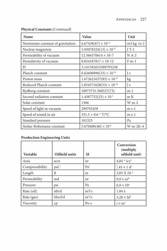
Appendices 227
Physical Constants (Continued)
Name Value Unit
Newtonian constant of gravitation 6.67428(67) × 10-11 m3 kg-1s-2
Nuclear magneton 5.05078324(13) × 10-27 J T-1
Permeability of vacuum 12.566370614 × 10⁻⁷ N A-2
Permittivity of vacuum 8.854187817 × 10⁻¹² F m-1
Pi 3.141592653589793238
Planck constant 6.62606896(33) × 10-34 J s
Proton mass 1.672621637(83) × 10-27 kg
Reduced Planck constant 1.054571628(53) × 10-34 J s
Rydberg constant 10973731.568527(73) m-1
Second radiation constant 1.4387752(25) × 10-2 m K
Solar constant 1366 W m-2
Speed of light in vacuum 299792458 m s-1
Speed of sound in air 331.5 + 0.6 * T/°C m s-1
Standard pressure 101325 Pa
Stefan-Boltzmann constant 5.670400(40) × 10-8 W m-2K-4
Production Engineering Units
Variable Oilfield units SI
Conversion
(multiply
oilfield unit)
Area acre nr 4,04 * icy1
Compressibility psL1 Pa1 ] 45 1 d4
Length ft m 3,05 X 10-L
Permeability md nr 9,9 ialfi
Pressure psi Pa 6,9 10s
Rate (oil) stb/d mVs 1.84 x
Rate (gas) Mscf/d m3/s 3,28 Id4
Viscosity cp Pa-s i m3

228 Formulas and Calculations for Drilling Operations
SI Units
SI base units
Base quantity SI base unit
Name of base quantity Symbol Name of SI base unit Symbol
Length l, x, r,etc. metre m
Mass m kilogram kg
time, duration t second s
electric current I, i ampere A
thermodynamic temperature T kelvin K
amount of substance n mole mol
luminous intensity Iv
candela cd
Examples of coherent derived units in the SI expressed in terms of base units
Derived quantity SI coherent derived unit
Name Symbol Name Symbol
Area A square metre m2
volume V cubic metre m3
speed, velocity v metre per second m s-1
acceleration a metre per second squared m s-2
wavenumber σ reciprocal metre m-1
density, mass density ρ kilogram per cubic metre kg m-3
surface density ρA
kilogram per square metre kg m-2
specific volume v cubic metre per kilogram m3kg-1
current density j ampere per square metre A m-2
magnetic field strength H ampere per metre A m-1
amount concentration,
concentration
c mole per cubic metre mol m-3
mass concentration ρ, γ kilogram per cubic metre kg m-3
luminance Lv
candela per square metre cd m-2
refractive index n (the number) one 1
relative permeability μr
(the number) one 1
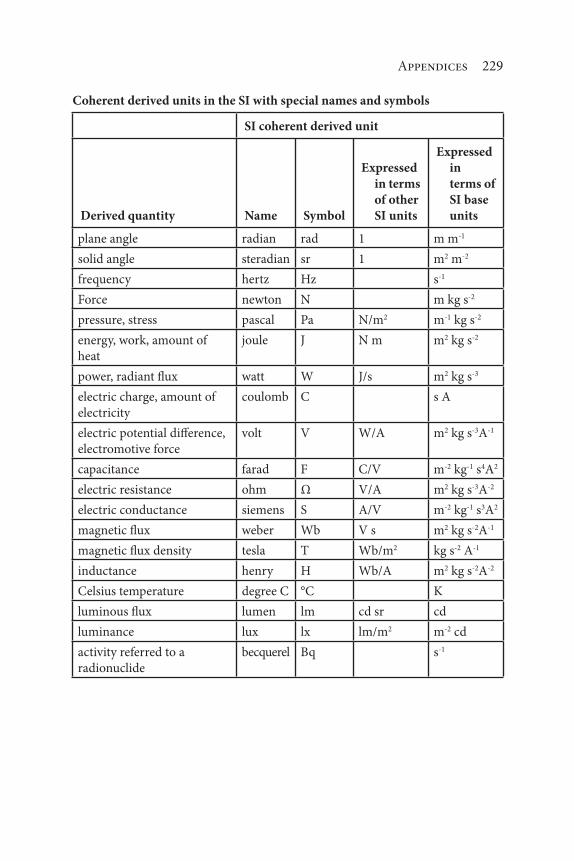
Appendices 229
Coherent derived units in the SI with special names and symbols
SI coherent derived unit
Derived quantity Name Symbol
Expressed
in terms
of other
SI units
Expressed
in
terms of
SI base
units
plane angle radian rad 1 m m-1
solid angle steradian sr 1 m2 m-2
frequency hertz Hz s-1
Force newton N m kg s-2
pressure, stress pascal Pa N/m2 m-1 kg s-2
energy, work, amount of
heat
joule J N m m2 kg s-2
power, radiant flux watt W J/s m2 kg s-3
electric charge, amount of
electricity
coulomb C s A
electric potential difference,
electromotive force
volt V W/A m2 kg s-3A-1
capacitance farad F C/V m-2 kg-1 s4A2
electric resistance ohm Ω V/A m2 kg s-3A-2
electric conductance siemens S A/V m-2 kg-1 s3A2
magnetic flux weber Wb V s m2 kg s-2A-1
magnetic flux density tesla T Wb/m2 kg s-2 A-1
inductance henry H Wb/A m2 kg s-2A-2
Celsius temperature degree C °C K
luminous flux lumen lm cd sr cd
luminance lux lx lm/m2 m-2 cd
activity referred to a
radionuclide
becquerel Bq s-1

230 Formulas and Calculations for Drilling OperationsE
xam
ple
s o
f S
I co
her
ent
der
ived
un
its
wh
ose
nam
es a
nd
sym
bo
ls i
ncl
ud
e S
I co
her
ent
der
ived
un
its
wit
h s
pec
ial
nam
es a
nd
sym
bo
ls
S
I co
her
ent
der
ived
un
it
Der
ived
qu
anti
tyN
ame
Sym
bo
lE
xp
ress
ed i
n t
erm
s o
f S
I b
ase
un
its
dyn
amic
vis
cosi
typ
asca
l sec
on
dP
a s
m–
1 k
g s–
1
mo
men
t o
f fo
rce
new
ton
met
reN
mm
2 k
g s–
2
surf
ace
ten
sio
nn
ewto
n p
er m
etre
N/m
kg
s–2
angu
lar
velo
city
rad
ian
per
sec
on
dra
d/s
m m
–1 s
–1 =
s–
1
angu
lar
acce
lera
tio
nra
dia
n p
er s
eco
nd
sq
uar
edra
d/s
2m
m–
1 s
–2 =
s–
2
hea
t fl
ux
den
sity
, irr
adia
nce
wat
t p
er s
qu
are
met
reW
/m2
kg
s–3
hea
t ca
pac
ity,
en
tro
py
jou
le p
er k
elvi
nJ/
Km
2 k
g s–
2 K
–1
spec
ific
hea
t ca
pac
ity,
sp
ecifi
c en
tro
py
jou
le p
er k
ilo
gram
kel
vin
J/(k
g K
)m
2 s
–2 K
–1
spec
ific
ener
gy
jou
le p
er k
ilo
gram
J/k
gm
2 s
–2
ther
mal
co
nd
uct
ivit
yw
att
per
met
re k
elvi
nW
/(m
K)
m k
g s–
3 K
–1
ener
gy
den
sity
jou
le p
er c
ub
ic m
etre
J/m
3m
–1 k
g s–
2
elec
tric
fiel
d s
tren
gth
volt
per
met
reV
/mm
kg
s–3 A
–1
elec
tric
ch
arge
den
sity
cou
lom
b p
er c
ub
ic m
etre
C/m
3m
–3 s
A

Appendices 231
surf
ace
char
ge d
ensi
tyco
ulo
mb
per
sq
uar
e m
etre
C/m
2m
–2 s
A
elec
tric
flu
x d
ensi
ty, e
lect
ric
dis
pla
cem
ent
cou
lom
b p
er s
qu
are
met
reC
/m2
m–
2 s
A
per
mit
tivi
tyfa
rad
per
met
reF
/mm
–3 k
g–1 s
4 A
2
per
mea
bil
ity
hen
ry p
er m
etre
H/m
m k
g s–
2 A
–2
mo
lar
ener
gy
jou
le p
er m
ole
J/m
ol
m2 k
g s–
2 m
ol–
1
mo
lar
entr
op
y, m
ola
r h
eat
cap
acit
yjo
ule
per
mo
le k
elvi
nJ/
(mo
l K
)m
2 k
g s–
2 K
–1 m
ol–
1
exp
osu
re (
x- a
nd
γ-r
ays)
cou
lom
b p
er k
ilo
gram
C/k
gk
g–1 s
A
abso
rbed
do
se r
ate
gray
per
sec
on
dG
y/s
m2 s
–3
rad
ian
t in
ten
sity
wat
t p
er s
tera
dia
nW
/sr
m4 m
–2 k
g s–
3 =
m2 k
g s–
3
rad
ian
cew
att
per
sq
uar
e m
etre
ste
rad
ian
W/(
m2sr
)m
2 m
–2 k
g s–
3 =
kg
s–3
cata
lyti
c ac
tivi
ty c
on
cen
trat
ion
kat
al p
er c
ub
ic m
etre
kat
/m3
m–
3 s
–1 m
ol

232 Formulas and Calculations for Drilling Operations
Non-SI units accepted for use with the International System of Units
Quantity
Name of
unit
Symbol for
unit Value in SI units
time, duration minute min 1 min = 60 s
hour h 1 h = 60 min = 3 600 s
day d 1 d = 24 h = 86 400 s
plane angle degree ° 1° = (π/180) rad
minute ‘ 1’ = (1/60)° = (π/10 800) rad
second “ 1” = (1/60)’ = (π/648 000) rad
area hectare ha 1 ha = 1hm2 = 104 m2
volume litre L, l 1 L = 1 dm3 = 10-3 m3
mass tonne t 1 t = 103 kg
Non-SI units whose values in SI units must be obtained experimentally
Quantity Name of unit
Symbol for
unit Value in SI units
Units accepted for use with the SI
energy electronvolt eV 1 eV = 1.602 176
53(14)×10-19 J
mass dalton Da 1 Da = 1.660 538
86(28)×10-27 kg
unified atomic mass unit u 1 u = 1 Da
length astronomical unit ua 1 ua = 1.495
978 706
91(6)×1011 m
Natural units (n.u.)
speed, velocity natural unit of speed
(speed of light in vacuum)
co
299 792 458 m s-1
action natural unit of action
(reduced Planck constant)
ħ 1.054 571
68(18)×10-34 Js
mass natural unit of mass (elec-
tron mass)
me
9.109 382
6(16)×10-31 kg
time, duration natural unit of time ħ/(mec
o2) 1.288 088 667
7(86)×10-21s
(Continued)

Appendices 233
Non-SI units whose values in SI units must be obtained experimentally
(Continued)
Quantity Name of unit
Symbol for
unit Value in SI units
Atomic units (a.u.)
charge atomic unit of charge,
(elementary charge)
e 1.602 176
53(14)×10-19 C
mass atomic unit of mass, (elec-
tron mass)
me
9.109 382
6(16)×10-31 kg
action atomic unit of action,
(reduced Planck constant)
ħ 1.054 571
68(18)×10-34 Js
length atomic unit of length, bohr
(Bohr radius)
ao
0.529 177 210
8(18)×10-10m
energy atomic unit of energy, har-
tree (Hartree energy)
Eh
4.359 744
17(75)×10-18 J
time, duration atomic unit of tim ħ/Eh
2.418 884 326
505(16)×10-17 s
Other non-SI units
Quantity Name of unit
Symbol for
unit Value in SI units
pressure bar bar 1 bar = 0.1 MPa = 105Pa
millimetre of
mercury
mmHg 1 mmHg ≈ 133.322 Pa
length angström 1 = 0.1 nm = 10-10 m
distance nautical mile M 1 M = 1852 m
area barn b 1 b = 100 fm2 = 10-28 m2
speed, velocity knot kn 1 kn = (1852/3600) m s-1
logarithmic ratio
quantities
neper Np
bel B
decibel dB

234 Formulas and Calculations for Drilling Operations
Non-SI units associated with the CGS system of units
Quantity
Name of
unit
Symbol for
unit Value in SI units
energy erg erg 1 erg = 10–7 J
force dyne dyn 1 dyn = 10–5 N
dynamic viscosity poise P 1 P = 1 dyn s cm–2 = 0.1 Pa s
kinematic viscosity stokes St 1 St = 1 cm2 s–1 = 10–4 m2 s–1
luminance stilb sb 1 sb = 1 cd cm–2 = 104 cd m–2
illuminance phot ph 1 ph = 1 cd sr cm–2 = 104 lx
acceleration gal Gal 1 Gal = 1 cm s–2 = 10–2 m s–2
magnetic flux maxwell Mx 1 Mx = 1 G cm2 = 10–8 Wb
magnetic flux density gauss G 1 G = 1 Mx cm–2 = 10–4 T
magnetic field œrsted Oe 1 Oe (103/4π) A m–1
SI prefixes
Factor Name Symbol Factor Name Symbol
101 deca da 10–1 deci d
102 hecto h 10–2 centi c
103 kilo k 10–3 milli m
106 mega M 10–6 micro μ
109 giga G 10–9 nano n
1012 tera T 10–12 pico p
1015 peta P 10–15 femto f
1018 exa E 10–18 atto a
1021 zetta Z 10–21 zepto z
1024 yotta Y 10–24 yocto y
Names and symbols for decimal multiples and submultiples of the unit of mass are formed by attaching prefix names to the unit name ‘gram’, and prefix symbols to the unit symbol ‘g’.
These SI prefixes refer strictly to powers of 10. They should not be used to indicate powers of 2 (for example, one kilobit represents 1000 bits and not 1024 bits). The names and symbols for the prefixes corresponding to 210, 220, 230, 240, 250, and 260 are, respectively: kibi, Ki; mebi, Mi; gibi, Gi; tebi, Ti; pebi, Pi; and exbi, Ei. Thus, for example, one kibibyte would be written: 1 KiB = 210 B = 1024 B, where B denotes a byte. Although these prefixes are

Appendices 235
not part of the SI, they should be used in the field of information technol-ogy to avoid the incorrect usage of the SI prefixes.
Sources: SPE. 1982. The SI Metric System of Units and SPE Metric Standard. Society of
Petroleum Engineers, Richardson, Texas.
The International System of Units (SI). Bureau International des Poids et Mesures,
Paris, France. 30 Nov 2010.
The International System of Units from NIST. Oct 2000. National Institute of
Standards and Technology. 30 Nov 2010. <http://physics.nist.gov/cuu/Units/>.
Decimal Multipliers for SI Prefixes
Prefix Origin Symbol
Multiplying
factor
yotla Greek or Latin ocio, “eight” Y 1024
zetta Latin sepictn, “seven” Z 102J
cx.a Greek hex, “six” E 1018
pet a Greek peme. “five” ‘ P 1015
tcra Greek reras. “monster” T 1012
gig* Greek gigas, “giant” G 109
mega Greek megas, “large” M 106
kilo Greek chilioi. “thousand” k 103
hccto Greek hekeson, “hundred” h 102
delta Greek deka, “ten” da 101
dcci Latin decimui, “fen th” d 10–1
centi Latin cemum, “hundred” c 10–2
mi lb Latin mille, “thousand” m 10–3
micro Latin micro- (Greek mUcros), “small” 10–6
nano Latin nanus (Greek flints j), “ dAarf ” n 10–9
pico Spanish pico, “a bit,” Italian piccolo, “small” P 10–12
femto Danish-Norwc gi an femten,” fifteen” f 10–15
alio Danish-Norwegian atten, “ eighteen” a 10–18
(Continued)

236 Formulas and Calculations for Drilling Operations
Decimal Multipliers for SI Prefixes (Continued)
Prefix Origin Symbol
Multiplying
factor
zepto Latin septem, “seven” z 10–21
yoelo Greek or Latin ocio, “eight” y 10–24
Common Unit Conversions
Gas Constant
0.082 lilcr-aLm/mole K
62.26 Jiler-mm Hg/
mole K
8.314 Joule/g-mole K
1.314 atm-ft3/lb-mole K
1.987 cal/g-mole K
1.987 Btu/lb-mole °R
0.73 atm-ft3/lb-mole °R
10.73 psi-fl3/lb-mole °R
1545 ft-lbf/lb-mole °R
Volume
1 ft3 = 28.316 liter
= 7.481 gal
1 in.3 = 16.39 cc
= 5.787 × 10⁻⁴ ft3
1 gal = 3.785 liter
= 8.34 lb H2O
1 m3 = 35.32 ft3
= 264.2 gal
Density
1 g/cm3 = 1000kg/m3
= 62.428 Ib/ft3
= 8.345 lb/gal
= 003613 lb/in.3
Length
1 mile = 1609 m = 5280 ft
1 fl = 30.48 cm = 12 in.
1 in. = 2.54 cm
1 im = 3.2808 ft
= 39.37 in.
1 nm= 10–9 m = 10 A
Viscosity
1 poise
= 6.7197 × 10⁻² lbm
/ft-sec
= 2.0886 × 10⁻³ lbf -sec/ft2
= 2.4191 × 10² lbm
/ft-hr
= 1 g/cm-scc
Conversion Factor
1 cal/g-mole = l.8Btu/
lb-mole
1 amu = 1.66063 10–24g
1 eV= 1.6022 10–24erg
1 radian = 57.3°
1 cm/sec= 1.9685 ft/min
1 rpm= 0.10472 ratlian/
sec
Pressure
1 aim = 101325 N/m2
= 14.696 psi
= 760 mmHg
= 29.921 in Hg
(32 °F)
= 33.91 ftH2O
(39.1 °F)
= 2116.2 lbf/ft2
= 1.0133 bar
= 1033.3 gf/cm2
Constant
h = 6.6262 10–27erg-sec
k = 1.38062 10–16 erg/K
N0= 6.022169 1023
C= 2.997925 1010 cm/
sec
F= 96487 coul/eq
e = 1.60219 10–19 coul
g = 980.665 cm/sec2
=32.174 ft/sec2
Mass
1 kg = 2.2046 lb
1 lb = 453.59 g
1 ton = 2000 lb
= 907.2 kg
1 B ton = 2240 lb
= 1016 kg
1 tonne = 2205 lb
= 1000 kg
1 slug = 32.2 lb
= 14.6 kg
(Continued)

Appendices 237
Common Unit Conversions (Continued)
Area
1 m2= 10.76 ft2 = 1550
in.2
1 ft2 = 929.0 cm2
Power
1 HP= 550 ft-lbf/sec
= 745.48 watt
1 Btu/hr = 0.293 watt
Force
1 N = 1 kg-m/sec2
= 102 dyne
= 0.22481 lbf
= 7.233 lbm
-ft/sec2
Transfer Coefficient
1 Btu/hr-ft2 F
= 5.6784 Joule/sec-m2
= 4.8825 Kcal/hr-m2 K
= 0.45362 Kcal/hr-ft2 K
= 1.3564 10–4 cal/sec-
cm2 K
1 lb/hr-ft2
= 1.3562 103 kg/sec-m2
= 4.8823 kg/hr-m2
= 0.45358 kg/hr-ft2
1 cal/g C = 1 Btu/Ibm
°F
= 1 Pcu/lbm
C
1 Btu/hr-ft °F
= 1.731 W/mK
= 1.4882 kcal/hr-m K
Energy & Work
1 cal = 4.184 Joule
1 Btu = 1055.1 Joule
= 252.16 cal
1 HP-hr = 2684500 Joule
= 641620 cal
= 2544.5 Btu
1 KW-hr = 3.6 106 Joule
= 860565 cal
= 3412.75 Blu
1 l-atm = 24.218 cal
1 fl-lbf= 0.3241 cal
1 Pcu = 453.59 cal
1 kg-m = 2.3438 cal
Stress
1 MPa = 145 psi
1 MPa = 0.102 kg/mm2
1 Pa= 10 dynes/cm2
1 kg/mm2= 9806 MPa
1 psi = 6.90 10–3 MPa
1 kg/mm2= 9.806 MPa
1 dyne/cm2 = 0.10 Pa
1 psi = 7.03 104 kg/
mm2
1 psi in.l/2 = 1.099 10–3
MPa ml/2
1 MPa ml/2 = 910 psi in.l/2
Water – Boiling Point Variation with Pressure
psia Boiling point, oF psia Boiling point, oF psia Boiling point, oF
0.5 79.6 44 273.1 150 358.5
1 101.7 46 275.8 175 371.8
2 126 48 278.5 200 381.9
3 141.4 50 281 225 391.9
4 125.9 52 283.5 250 401
5 162.2 54 285.9 275 409.5
6 170 56 288.3 300 417.4
7 176.8 58 290.5 325 424.8
8 182.8 60 292.7 350 431.8
9 188.3 62 294.9 375 438.4
10 193.2 64 297 400 444.7
11 197.7 66 299 425 450.7
12 201.9 68 301 450 456.4(Continued)

238 Formulas and Calculations for Drilling Operations
Water – Boiling Point Variation with Pressure (Continued)
psia Boiling point, oF psia Boiling point, oF psia Boiling point, oF
13 205.9 70 303 475 461.9
14 209.6 72 304.9 500 467.1
14.69 212 74 306.7 525 472.2
15 213 76 308.5 550 477.1
16 216.3 78 310.3 575 481.8
17 219.4 80 312.1 600 486.3
18 222.4 82 313.8 625 490.7
19 225.2 84 315.5 650 495
20 228 86 317.1 675 499.2
22 233 88 318.7 700 503.2
24 237.8 90 320.3 725 507.2
26 242.3 92 321.9 750 511
28 246.4 94 323.4 775 514.7
30 250.3 96 324.9 800 518.4
32 254.1 98 326.4 825 521.9
34 257.6 100 327.9 850 525.4
36 261 105 331.4 875 528.8
38 264.2 110 334.8 900 532.1
40 267.3 115 338.1 950 538.6
42 270.2 120 341.3 1000 544.8
Water – Density and Viscosity in Relation to Temperature
T, oC Density, kgm/cubic meter Viscosity, mPa
0 1000 1.788
10 1000 1.307
20 998 1.003
30 996 0.799
40 992 0.657
50 988 0.548
60 983 0.467
70 978 0.405
(Continued)

Appendices 239
Water – Density and Viscosity in Relation to Temperature (Continued)
T, oC Density, kgm/cubic meter Viscosity, mPa
80 972 0.355
90 965 0.316
100 958 0.283
Water Temperature and Vapor Pressure
Temperature Vapor Pressure
F C psi ll
40 4.4 0.12 0.28
50 10 0.18 0.41
60 15.6 0.26 0.59
70 21.1 0.36 0.82
SO 26.7 0.51 1.17
90 32.2 0.70 1.61
100 37.8 0.95 2.19
110 43.3 1.28 2.94
120 48.9 1.69 3.91
130 54.4 2.22 5.15
140 60 2.89 6.68
150 65.6 3.72 8.56
160 71.1 4.74 10.95
170 76.7 5.99 13.84
I8O 82.2 7.51 17.35
190 87.8 9.34 21.55
200 93.3 11.50 26.65
212 100 14.70 33.96
Weights and Measures – General
Unit of Measure Equivalent
Barrel 31.5 gallons
Bushel 2150.4 cubic inches
Bushel (dry) 4 pecks
Centimeter 0.39 inches
(Continued)

240 Formulas and Calculations for Drilling Operations
Weights and Measures – General (Continued)
Unit of Measure Equivalent
Cord 128 cubic feet
Cord 4 cubic meters
Cubic centimeter 0.061 cubic inches
Cubic foot 283.17 cubic centimeters
Cubic foot 1728 cubic inches
Cubic inch 16.39 cubic centimeters
Cubic meter 1.31 cubic yards
Cubic yard3 0.77 cubic meters
Foot 30.48 centimeters
Gallon (us) 231 cubic inches
Grain 0.002 ounces
Gram 0.04 ounces
Hectare 2.47 acres
Hogshead 2 barrels
Inch 2.54 centimeters
Kilogram 2.21 pounds
Meter 1.09 yards
Mile 1.61 kilometers
Ounce 28.35 grams
Peck 8 quarts
Pound 0.45 kilograms
Pound (troy) 12 ounces
Square centimeter 0.16 square inches
Square foot 0.09 square meters
Square inch 6.45 square centimeters
Square meter 1.2 square yards
Square mile 2.59 square kilometers
Square yard square 0.84 meters
Ton (long) 2240 pounds
Ton (metric) 2200 pounds
Ton (shipping) 40 feet3
Ton (short) 2000 pounds
(Continued)

Appendices 241
Weights and Measures – General (Continued)
Unit of Measure Equivalent
Township 36 square miles (93 square kilometers)
Yard 0.91 meters

243
Glossary
Abnormal pressure: A formation pore pressure that is higher than that resulting from a water gradient.
Absolute temperature: Temperature related to absolute zero, the tempera-ture at which all molecular activity ceases; calculated by adding 460oF to the temperature in Fahrenheit to obtain the absolute temperature in degrees Rankine or by adding 273oC to the temperature in degrees Celsius to obtain the absolute temperature in degrees Kelvin.
Absorption: The penetration or apparent disappearance of molecules or ions of one or more substances into the interior of a solid or liquid.
Accumulator: A hydraulic accumulator is a pressure storage reservoir in which a non-compressible hydraulic fluid is held under pressure that is applied by an external source; an accumulator enables a hydraulic system to cope with extremes of demand using a less powerful pump, to respond more quickly to a temporary demand, and to smooth out pulsations; compressed gas accumulators, also called hydro-pneumatic accumulators, are the most common type of accumulators.
Acid: Any chemical compound containing hydrogen capable of being replaced by elements or radicals to form salts; a compound, which, on
Formulas and Calculations for Drilling Operations, Second Edition.James G. Speight.
© 2018 Scrivener Publishing LLC. Published 2018 by John Wiley & Sons, Inc.

244 Glossary
dissociation in solution, yields excess hydrogen ions; acids lower the pH. Examples of acids or acidic substances are hydrochloric acid (HCl), sodium acid pyrophosphate (SAPP), and sulfuric acid (H
2SO
4).
Acidity: The relative acid strength of liquid as measured by pH; a com-pounds having a pH value below 7.
Active system: The volume of drilling fluid being circulated to drill a hole; consists of the volume of drilling fluid in the wellbore plus the volume of drilling fluid in the surface tanks through which the fluid circulates.
Adhesion: The force that holds unlike molecules together.Adsorb: see Adsorption.Adsorbed chemical: The molecular species that adhere to the surfaces of
solid particles that cannot be removed by draining, even with centrifu-gal force.
Adsorption: A surface phenomenon exhibited by a solid (adsorbent) to hold or concentrate gases, liquids, or dissolved substances (adsorp-tive) upon its surface; for example, water held to the outside surface of hydrated bentonite, is adsorbed water.
Aerated fluid: Drilling fluid to which air or gas has been deliberately added to lighten the fluid column.
Aeration: The technique of injecting air or gas in varying amounts into a drilling fluid to reduce the hydrostatic head; also, the inadvertent mechanical incorporation and dispersion of air or gas into a drilling fluid.
Agglomeration: A group of two or more individual particles held together by strong forces; typically, agglomerates are stable to normal stirring, shaking, or handling as powder or a suspension.
Aggregate: To gather together, to clump together; a flocculated drilling fluid will aggregate if flocculent is added.
Aggregation: Formation of aggregates; in drilling fluids, aggregation results in the stacking of the clay platelets face to face and, consequently, the viscosity and gel strength of the fluid decreases.
Agitation: The process of rapidly mixing a slurry within a tank to obtain and maintain a uniform mixture.
Agitator: A mechanically driven impeller used to stir the drilling fluid to assist in the suspension of solids, blending of additives, and mainte-nance of uniform consistency.
Air cutting: The inadvertent mechanical incorporation and dispersion of air into a drilling fluid system.
Airlock: A condition causing a centrifugal pump to stop pumping because of a large bubble of air or gas in the center of the pump impeller which prevents the liquid from entering the pump suction.

Glossary 245
Alkali: Any compound having pH properties higher than the neutral state, i.e., pH >7.
Alkalinity: The combining power of a base measured by the maximum number of equivalents an acid with which it can react to form a salt; in water analyses, alkalinity typically represents the carbonates, bicarbon-ates, hydroxides, and occasionally the borate, silicates, and phosphates in the water.
Alum: Aluminum sulfate, Al2(SO
4)
3 which is a common inorganic coagulant.
Aluminum stearate: An aluminum salt of stearic acid used as a defoaming agents.
Amorphous: The property of a solid substance that does not crystallize and is without any definite characteristic shape.
Anhydrite: A mineral compound, CaSO4, that is often encountered while
drilling; may occur as thin stringers or massive formations.Anhydrous: Without water.Aniline point: The lowest temperature at which equal volumes of freshly
distilled aniline and an oil sample that is being tested are completely miscible; gives an indication of the molecular characteristics (paraffinic, naphthenic, asphaltic, aromatic) of the oil.
Anion: A negatively charged atom or radical, such as chloride (Cl–), hydroxide (OH–), and sulfate (SO4-) in solution of an electrolyte; anions move toward the anode (positive electrode) under the influence of an electrical potential.
Annular pressure loss: The pressure on the annulus required to pump the drilling fluid from the bottom of the hole to the top of the hole in the annular space.
Annular velocity: The velocity of a fluid moving in the annulus, usually expressed in ft/min or m/min.
Annulus (annular space): The space between the drill string and the wall of the wellbore or the inside surface of the casing.
API fluid loss: This fluid loss is measured under ambient conditions – usu-ally room temperature and 100 psi differential pressure.
API gravity: The gravity (weight per unit volume) of crude oil or other related fluids as measured by a system recommended by the American Petroleum Institute (API).
Apparent viscosity: The apparent viscosity in centipoise, as determined by the direct-indicating viscometer is equal to one-half the 600-rpm reading.
Axial flow: Flow from a mechanical agitator in which the fluid first moves along the axis of the impeller shaft (usually down toward the bottom of a tank) and then away from the impeller.

246 Glossary
Backpressure: The frictional or blocking pressure opposing fluid flow in a conduit.
Back tank: The compartment on a shale shaker that receives drilling fluid from the flowline.
Backing plate: The plate attached to the back of screen cloth(s) for support.
Baffles: Plates or obstructions built into a compartment to change the direction of fluid flow.
Balanced design hydrocyclone: A hydrocyclone that has the lower apex adjusted to the diameter of the cylinder of air formed within the cone by the cyclonic forces of drilling fluid spinning within cone.
Barium sulfate (BaSO4): used for increasing the density of drilling fluids;
barite is the naturally-occurring mineral):Barrel (bbl): A volumetric unit of measure used in the petroleum industry
consisting of 42 U.S. gallons.Barrel equivalent: One gram of material in 350 ml of fluid is equivalent to
a concentration of 1 lb of that material in an oilfield barrel of fluid.Base: A compound of a metal, or a metal-like group, with hydrogen and
oxygen in the proportions that form an OH– radical, when ionized in an aqueous solution, yielding excess hydroxyl ions; examples of bases are sodium hydroxide (caustic soda, NaOH) and calcium hydroxide [Ca(OH)
2].
Base exchange: The replacement of the cations associated with the surface of a clay particle by another species of cation, for example, the substi-tution of sodium cations by calcium cations on the surface of a clay particle.
Basicity: pH value above 7; the ability to neutralize or accept protons from acids.
Bernoulli Principle: The principle demonstrates that the sum of pres-sure and velocity through or over a device represents equal quantities, neglecting the effects of losses due to friction and/or increases by add-ing energy with external devices such as pumps.
Bicarb: Sodium bicarbonate, NaHCO3.
Bingham model: A mathematical description that relates shear stress to shear rate in a linear manner; the model requires only two constants (plastic viscosity and yield point) and is the simplest rheological model possible to describe a non-Newtonian liquid.
Blooie line: The flowline for air or gas drilling.Blowout: An uncontrolled escape of drilling fluid, gas, oil, or water from
the well; caused by the formation pressure being greater than the hydro-static head of the fluid being circulated in the well bore.

Glossary 247
Bottom flooding: The behavior of a hydrocyclone when the underflow discharges whole drilling fluid rather than separated solids.
Brackish water: Water containing low concentrations of any soluble salts.Break circulation: Commencement of movement of the drilling fluid after
it has been quiescent in a borehole.Brine: Water containing a high concentration of common salts such as
sodium chloride, calcium chloride, magnesium chloride, calcium bro-mide, and zinc bromide.
Buffer: Any substance or combination of substances that, when dissolved in water, produces a solution that resists a change in its hydrogen ion concentration upon the addition of an acid or base.
Cable tool drilling: A method of drilling a well by allowing a weighted bit (or chisel) at the bottom of a cable to fall against the formation being penetrated.
Calcium: One of the alkaline earth elements with a valence of 2 and an atomic weight of 40; a component of lime, gypsum, and limestone; cal-cium compounds are a common cause of the hardness of water.
Calcium carbonate: CaCO3. An acid soluble calcium salt sometimes used
as a weighting material (such as limestone and oyster shell) in special-ized drilling fluids.
Calcium chloride: CaCl2. A very soluble calcium salt sometimes added to
drilling fluids to impart special inhibitive properties, but used primarily to increase the density of the liquid phase (water) in completion fluids and as an inhibitor to the water phase of invert oil emulsion drilling fluids.
Calcium hydroxide: Ca(OH)2. The active ingredient of slaked lime; also,
the main constituent in cement (when wet) and is often referred to as ‘‘slaked lime’’ in field terminology.
Calcium sulfate: Anhydrite, CaSO4, plaster of Paris, CaSO
4.12H
2O, and
gypsum, CaSO4.2H
2O; occurs in drilling fluids as a contaminant or may
be added as a commercial product to certain drilling fluids to impart special inhibitive properties to the fluid.
Calcium-treated drilling fluids: Drilling fluids to which quantities of sol-uble calcium compounds have been added or allowed to remain from the formation drilled to impart special inhibitive properties to the drill-ing fluid.
Capacity: The maximum volume flow rate at which a solids-control device is designed to operate without detriment to separation.
Cascade: Gravity-induced flow of fluid from one unit to another.Casing: Steel pipe placed in an oil or gas well to prevent the wall of the
wellbore in a drilled interval from caving in, as well as to prevent move-ment of fluids from one formation to another.

248 Glossary
Cation: The positively charged particle in the solution of an electrolyte, which, under the influence of an electrical potential, moves toward the cathode (negative electrode); examples are Na+, H+, NH
4+, Ca2+, Mg2+,
and Al3+.Cation exchange capacity: The total amount of cations adsorbed on the
basal surfaces or broken bond edges of a clay sample, expressed in mil-liequivalents per 100 grams of dry clay.
Caustic: Sodium hydroxide, NaOH.Caustic soda: Sodium hydroxide, NaOH; an alkali.Cavitation: The formation and collapse of low-pressure bubbles in a liq-
uid; cavitation occurs in centrifugal pumps when the pressure within the impeller chamber decreases below the vapor pressure of the liquid.
Cement: A mixture of calcium aluminate derivatives and calcium silicate derivatives made by combining lime and clay while heating; slaked cement contains about 62.5% calcium hydroxide, which can cause a major prob-lem when cement contaminates drilling fluid; used to hold the casing in place and to prevent fluid migration between subsurface formations and it is necessary to know the numbers of sacks of cement required.
Cement plug: The cement plug is part of the well completion process in which a plug of cement slurry placed in the wellbore. Cement plugs are also used for a variety of applications including hydraulic isolation, provision of a secure platform, and in window-milling operations for sidetracking a new wellbore.
Cement sack: The sack, which is a unit of measure for Portland cement in the United States, refers the amount of cement that occupies a bulk volume of 1.0 ft3. For most Portland cement, including API classes of cement, a sack weighs 94 pounds.
Centipoise (cP): Unit of viscosity equal to 0.01 Poise; the poise equals 1 dyne-second per square centimeter; as an example, the viscosity of water at 20oC (68oF) is 1.005 cP (1 cP = 0.000672 lb/ft sec).
Chemical treatment: The addition of chemicals (such as caustic or thin-ners) to the drilling fluid to adjust the drilling fluid properties.
Clay: A soft, variously colored earth, commonly hydrous silicates of alu-mina, formed by the decomposition of feldspar and other aluminum silicates; insoluble in water but disperse under hydration, grinding, or velocity effects; shearing forces break down the clay particles to sizes varying from submicron particles to particles 100 microns or larger.
Clay-size particle: a solid particle having an equivalent spherical diameter less than 2 microns.
Closed loop mud systems: A drilling-fluid processing system that mini-mizes the liquid discard.

Glossary 249
Closed loop systems (pressurized): A system in which formation fluid is contained in tanks and not exposed to the atmosphere until it is sent to the flare line or to the holding tank.
Coagulation: The destabilization and initial aggregation of colloidal and finely divided suspended matter by the addition of a floc-forming agent.
Coalescence: The change from a liquid to a thickened curd-like state by chemical reaction; the combination of globules in an emulsion caused by molecular attraction of the surfaces.
Coarse solids: Solids larger than 2000 microns in diameter.Connate water: Water trapped within sedimentary deposits, particularly
as hydrocarbons displaced most of the water from a reservoir.Contact time: The time required for a specific fluid to pass a designated
depth or point in the annulus during pumping operations; normally used as a design criterion for mud removal in turbulent flow.
Contamination: In a drilling fluid, the presence of any material that may tend to harm the desired properties of the drilling fluid.
Continuous phase: The fluid phase that surrounds the dispersed phase; also, the fluid phase of a drilling fluid, either water, oil, or synthetic oil – the dispersed (non-continuous) phase may be solid or liquid.
Conventional drilling fluid: A drilling fluid containing essentially clay and water; also called conventional mud.
Created fractures: Induced fractures by means of hydraulic or mechanical pressure exerted on the formation by the drill string and/or circulating fluid.
Critical velocity: That velocity at the transitional point between laminar and turbulent types of fluid flow; this point occurs in the transitional range of Reynolds numbers between approximately 2000 to 3000.
Cut point: Cut point curves are developed by dividing the mass of solids in a certain size range removed by the total mass of solids in that size range that enters the separation device.
Cuttings: The pieces of formation dislodged by the bit and brought to the surface in the drilling fluid.
Cyclone: A device for the separation of solid particles from a drilling fluid; the most common cyclones used for solids separation are a desander or desilter.
Darcy: A unit of permeability; for example, a porous medium has a perme-ability of 1 Darcy when a pressure of 1 atm on a sample 1 cm long and 1 sq cm in cross section will force a liquid of 1 cP viscosity through the sample at the rate of 1 cc per sec.
De-duster: A tank at the end of the blooie line in air or gas drilling in which water is injected to settle the dust caused by drilling.

250 Glossary
Deflocculant: A chemical that promotes deflocculation or inhibits flocculation.
Defoamer: Any substance used to reduce or eliminate foam by reducing the surface tension of a liquid.
Degasser: A device that removes entrained gas from a drilling fluid, espe-cially the very small bubbles that do not float readily in viscous drilling fluid.
Dehydration: Removal of free or combined water from a compound or mixture.
Deliquescence: The liquification of a solid substance due to the solution of the solid by absorption of moisture from the air, for example, calcium chloride deliquesces in humid air.
Density: Mass per unit volume expressed in pounds per gallon (ppg), grams per cubic (g/cc), or pounds per cubic ft (lb/cu ft); drilling-fluid density is commonly referred to as mud weight.
Desand: To remove most API sand (>74 microns) from drilling fluid.Desander: A hydrocyclone larger that can remove a very high proportion
of solids larger than 74 micrometers.Desilt: To remove most silt particles greater than 15 to 20 microns from an
unweighted fluid.Desilter: A hydrocyclone which can remove a large fraction of solids larger
than 15 to 20 microns.Destabilization: A condition in which colloidal particles no longer remain
separate and discrete, but contact and agglomerate with other particles.Diatomaceous earth: A very porous natural earth compound composed
of siliceous skeletons; sometimes used for controlling lost circulation and seepage losses and as an additive to cement.
Differential pressure: The difference in pressure between two points; typi-cally, the difference in pressure at a given point in the well bore between the hydrostatic pressure of the drilling-fluid column and the formation pressure; the differential pressure can be positive, zero, or negative with respect to the formation pressure.
Differential sticking: Differential sticking is a condition whereby the drill string cannot be moved (rotated or reciprocated) along the axis of the wellbore and typically occurs when high-contact forces caused by low reservoir pressure, high wellbore pressure, or both, are exerted over a sufficiently large area of the drillstring; differential sticking is a product of the differential pressure between the wellbore and the reservoir and the area that the differential pressure is acting upon; a relatively low dif-ferential pressure (Δp) applied over a large working area can be just as

Glossary 251
effective in sticking the pipe as can a high differential pressure applied over a small area.
Diffusion: The spreading, scattering, or mixing of material (gas, liquid, or solid).
Dilatant fluid: dilatant or inverted plastic fluid is usually made up of a high concentration of well-dispersed solids that exhibit a nonlinear consistency curve passing through the origin; the apparent viscosity increases instantaneously with increasing shear rate and the yield point, as determined by conventional calculations from the direct-indicating viscometer readings, is negative.
Diluent: Liquid added to dilute (thin) a solution or suspension.Dilution factor: The ratio of the actual volume of drilling fluid required to
drill a specified interval of footage using a solids-removal system ver-sus a calculated volume of drilling fluid required to maintain the same drilled-solids fraction over the same specified interval of footage with no drilled-solids removal.
Dilution rate: The rate, in gpm or bbl/hr, at which fluids and/or premix is added to the circulating system for solids management.
Dilution ratio: The ratio of the volume of dilution liquid to the volume of raw drilling fluid in the feed prior to entering a liquid/solids separator.
Dilution water: Water used for dilution of water-based drilling fluid.Discharge: Material removed from a system; also called effluent.Dispersant: A chemical that promotes dispersion of particles in a fluid; a
deflocculant is often referred to (inaccurately) as a dispersant.Dispersed phase: The scattered phase (solid, liquid, or gas) of a dispersion;
the particles are finely divided and surrounded by the continuous phase.Disassociation: The splitting of a compound or element into two or more
simple molecules, atoms, or ions.Dog leg (dogleg): The elbow caused by a sharp change of drilling direction
in the well bore.Dolomite: A mineral that is a mixture of calcium carbonate and magne-
sium carbonate; CaCO3.MgCO
3.
Drill bit (drillbit): The cutting or boring element at the end of the drill string.
Drilled solids: Formation solids that enter the drilling-fluid system, whether produced by a bit or from the side of the borehole.
Drilled-solids fraction: The average volume fraction of drilled solids maintained in the drilling fluid over a specified interval of footage.
Drilled-solids removal system: All equipment and processes used while drilling a well that remove the solids generated from the hole and carried

252 Glossary
by the drilling fluid, that is, settling, screening, desanding, desilting, centrifuging, and dumping.
Driller’s method: The Driller’s Method requires two circulations: during the first circulation, the influx is circulated out with the original mud weight. Constant bottom hole pressure is maintained by holding circu-lating drill pipe pressure constant through the first circulation. See Kill methods.
Drilling cost: The drilling is a summation of several variable, such as the right to enter and drill on the property owner’s land is accomplished by obtaining a lease. The lease is subject to title search and proper record-ing in much the same way as real estate. Between legal cost for title work and lease bonus wells see costs in excess of $1,000,000 for leasing alone.
Drill stem test (DST): A post-drilling and preproduction test that allows formation fluids to flow into the drill pipe under controlled conditions, to determine whether oil and/or gas in commercial quantities have been encountered in the penetrated formations.
Drill string (drillstring): The column of drill pipe with attached tool joints that transmits fluid and rotational power from the kelly to the drill col-lars and bit.
Drilling fluid: Term applied to any liquid or slurry pumped down the drill string and up the annulus of a hole to facilitate drilling; also called drill-ing mud or mud.
Drilling-fluid additive: Any material added to a drilling fluid to achieve a desired effect.
Drilling-fluid analysis: Examination and testing of the drilling fluid to determine its physical and chemical properties and functional ability.
Drilling-fluid cycle time: The time necessary to move a fluid from the kelly bushing to the flowline in a borehole. The cycle, in minutes, equals the barrels of drilling fluid in the hole minus pipe displacement divided by barrels per minute of circulation rate.
(Holebbl
- Pipe Voumebbl
) = Circulation Ratebbl/min
Drilling in: The drilling operation starting at the point of drilling into the producing formation.
Drilling mud: Drilling fluid.Drilling out: The operation of drilling out of the casing shoe after the
cementing of a casing or liner in place; drilling out of the casing is done before further hole is made or completion attempted.
Drilling rate: The rate at which hole depth progresses, expressed in linear units per unit of time (including connections) as feet/minute or feet/hour.

Glossary 253
Dry bottom: An adjustment to the underflow opening of a hydrocyclone that causes a dry beach, usually resulting in severe plugging.
Dry plug: The plugging of the underflow opening of a hydrocyclone caused by operating with a dry bottom.
Effective screening area: The portion of a screen surface available for sol-ids separation.
Effluent: A discharge of liquid; generally, a stream of liquid after separa-tion or purification; also called discharge.
Electric logging: Logs run on a wire line to obtain information concerning the porosity, permeability, density, and/or fluid content of the forma-tions drilled; the drilling-fluid characteristics may need to be altered to obtain good logs.
Electrolyte: A substance that dissociates into charged positive and negative ions when in solution or a fused state; an electrolyte will then conduct an electric current and acids, bases, as well as salts are common electrolytes.
Elevation head: The pressure created by a given height of fluid; also called hydrostatic pressure head.
Emulsifier: A chemical substance used to produce a mixing of two liquids that do not solubilize in each other or maintain a stable mixture when agitated in the presence of each other.
Emulsion: A substantially permanent heterogeneous mixture of two or more liquids that do not normally dissolve in each other but are held in a dispersed state, one within the other; the dispersion is accomplished by the combination of mechanical agitation and presence of fine solids and/or emulsifiers.
Encapsulation: The process of totally enclosing electrical parts or circuits with a polymeric material (usually epoxy resin).
End point: Indicates the end of a chemical testing operation when a clear and definite change is observed in the test sample; in titration, this change is frequently a change in color of an indicator or marker added to the solution, or the disappearance of a colored reactant.
Equivalent circulating density (ECD): The effective drilling-fluid weight at any point in the annulus of the well bore during fluid circulation; includes drilling-fluid density, cuttings in the annulus, and annular pressure loss.
Equivalent spherical diameter (ESD): The theoretical dimension usually referred to when the sizes of irregularly shaped particles are discussed; these dimensions can be determined by several methods, such as set-tling velocity, electrical resistance, and light reflection.
Equivalent weight: The atomic weight or formula weight of an ele-ment, compound, or ion divided by its valence; elements entering into

254 Glossary
chemical combination or chemical reaction always do so in quantities to their equivalent weights; also known as combining weight.
Expected cost: The probability that a certain cost will be incurred.Expected profit is the probability of receiving a certain profit.Expected value: The difference between expected profits and expected
costs. See also: Future value.Fault: Geological term denoting a formation break across the trend of a
subsurface strata; faults can significantly affect the drilling fluid and cas-ing programs due to possibilities for lost circulation, sloughing hole, or kicks.
Feed (feedstock): A mixture entering a liquid/solids separation device or a reactor.
Feed capacity (feedstock capacity): The maximum volume flow rate at which a solids-control device is designed to operate without detriment to separation efficiency; the capacity will be dependent on particle size, particle concentration, viscosity, and other variables of the feed (feedstock).
Feed chamber: That part of a device that receives the mixture of diluents, drilling fluid, and solids to be separated.
Feed head: The equivalent height, in feet or meters, of a column of fluid at the cyclone feed header.
Feed header: A pipe, tube, or conduit to which two or more hydrocy-clones have been connected and from which they receive their feed slurry.
Feed inlet: The opening through which the feed fluid enters a solids sepa-ration device. Also known as feed opening.
Feed pressure: The actual gauge pressure measured as near as possible to, and upstream of, the feed inlet of a device.
Filter cake: The suspended solids that are deposited on the filter during the process of filtration.
Filter cake texture: The physical properties of a cake as measured by toughness, slickness, and brittleness.
Filtrate: The liquid that is forced through a porous medium during the filtration process.
Filter press: A device for determining the fluid loss of a drilling fluid.Filter run: The interval between two successive backwashing operations
of a filter.Filterability: The characteristic of a clear fluid that denote both the ease of
filtration and the ability to remove solids while filtering.Fine solids: Solids 44 to 74 microns in diameter, or sieve size 325 to 200
mesh.

Glossary 255
Fishing: Operations on the rig for retrieving sections of pipe, collars, or other obstructive items that are in the wellbore and would interfere with drilling or logging operations.
Flat gel: A condition wherein the gel strength does not increase apprecia-bly with time and is essentially equal to the initial gel strength; opposite of progressive gel.
Floc: Small masses of gelatinous solids formed in a liquid.Flocculates: A group of aggregates or particles in a suspension formed by
electrostatic attraction forces between negative and positive charges.Flocculating agent: Substances, for example, most electrolytes, a few poly-
saccharides, certain natural or synthetic polymers, that bring about the thickening of a drilling fluid; in Bingham plastic fluids, the yield point and gel strength increase with flocculation.
Flooding: The effect created when a screen, hydrocyclone, or centrifuge is fed beyond its capacity; flooding may also occur on a screen because of blinding.
Flowback pan: A pan or surface below a screen that causes fluid passing through one screen to flow back to the feed end of a lower screen.
Flow capacity: The rate at which a shaker can process drilling fluid and solids; depends on many variables, including shaker configuration, design and motion, drilling fluid rheology, solids loading, and blinding by near-size particles.
Flow drilling: Drilling in which there is a constant flow of formation fluid.Flowline: The pipe (usually) or trough that conveys drilling fluid from the
rotary nipple to the solids-separation section of the drilling fluid tanks on a drilling rig.
Flow rate: The volume of liquid or slurry moved through a pipe in one unit of time, such as gpm or bbl/min.
Flow streams: With respect to centrifugal separators, all liquids and slur-ries entering and leaving a machine, such as feed drilling fluid stream plus dilution stream equals overflow stream plus underflow stream.
Fluid: Any substance that will readily assume the shape of the container in which it is placed; includes both liquids and gases; a substance in which the application of every system of stress (other than hydrostatic pressure) will produce a continuously increasing deformation without any relation between time rate of deformation at any instant and the magnitude of stress at the instant.
Fluid flow: The state of dynamics of a fluid in motion as determined by the type of fluid (e.g., Newtonian plastic, pseudoplastic, dilatant), the properties of the fluid such as viscosity and density, the geometry of the system, and the velocity; under a given set of conditions and fluid

256 Glossary
properties, the fluid flow can be described as plug flow, laminar (called also Newtonian, streamline, parallel, or viscous) flow, or turbulent flow.
Fluid loss: The relative amount of fluid loss (filtrate) through permeable formations or membranes when the drilling fluid is subjected to a pres-sure differential.
Fluidity: The reciprocal of viscosity; the ease of flowing; the measure of rate with which a fluid is continuously deformed by a shearing stress.
Fluorescence: Instantaneous re-emission of light of a greater wavelength than that of the light originally absorbed.
Flute: A curved metal blade wrapped around a shaft as on a screw con-veyor in a centrifuge.
Foam: A two-phase system that is similar to an emulsion, in which the dispersed phase is a gas or air; bubbles (usually air but can be formation gas) floating on the surface of the drilling fluid.
Foaming agent: A substance that produces stable bubbles at the air/liquid interface due to agitation, aeration, or ebullition; in air or gas drilling, foaming agents are added to turn water influx into aerated foam; com-monly referred to as “mist drilling”.
Foot: Unit of length (12 inches) in British (foot-pound-second) system.Foot-pound: Unit of work or of mechanical energy, which is the capacity
to do work; 1 foot is the work performed by a force of 1 pound act-ing through a distance of 1 foot; or the work required to lift a 1-pound weight a vertical distance of 1 foot.
Foot valve: A check valve installed at the suction end of a suction line.Formation: A bed or deposit (stratum) composed throughout of substan-
tially the same type of rock (mineral).Formation damage: Damage caused by the invasion of the formation by
drilling-fluid particles, drilling-fluid filtrates, and/or cement filtrates; can also result from changes in pH and a variety of other conditions; asphaltene constituents deposited from crude oil will also damage some formations.
Formation fluid: The fluid (brine, oil, gas) that exists in the pores of a formation.
Formation sensitivity: The tendency of certain producing formations to adversely react with the drilling and completion process.
Free liquid: The liquid film that can be removed by gravity draining or centrifugal force.
Free-water knockout: A water/gas separator ahead of the flare line.Freshwater drilling fluid: A drilling fluid in which the liquid phase is
freshwater.

Glossary 257
Future value: The value of a current asset at a specified date in the future based on an assumed rate of growth over time. See also: Expected value.
Using simple interest, future value = P x I x N where P is the initial investment amount, I is the interest rate and N is the number of years the investment will be held.
For compound interest, the future value = P x [(1 + I)N – 1] where P is the principal, I = nominal annual interest rate, and N = the number of compounding periods.
Galena: Lead sulfide (PbS); technical grades (specific gravity about 7.0) are used for increasing the density of drilling fluids to points impractical or impossible with barite. Almost entirely used in preparation of kill fluids.
Gas buster: Mud/gas separator.Gas cut: Gas entrained by a drilling fluid.Gel: A state of a colloidal suspension in which shearing stresses below a cer-
tain finite value fail to produce permanent deformation; the minimum shearing stress that will produce permanent deformation is known as the shear or gel strength of the gel; also, a term used to designate highly colloidal, high-yielding, viscosity-building, commercial clays, such as bentonite and attapulgite.
Gelation: Association of particles forming continuous structures at low shear rates.
Gel cement: Cement having a small to moderate percentage of bentonite added as a filler and/or reducer of the slurry weight; the bentonite may be dry-blended into the mixture or added as a prehydrated slurry.
g Factor: The acceleration of an object relative to the acceleration of gravity.g Force: The centrifugal force exerted on a mass moving in a circular path.Gypsum: Calcium sulfate, CaSO
4.2H2O, frequently encountered while
drilling; may occur as thin stringers or in massive formations.Head: The height a column of fluid would stand in an open-ended pipe if it
was attached to the point of interest; the head at the bottom of a 1000-ft well is 1000 ft, but the pressure would be dependent on the density of the drilling fluid in the well.
Heterogeneous: A substance that consists of more than one phase and is not uniform, such as colloids, emulsions, and has different properties in different parts.
High-gravity solids (HGS): Solids purchased and added to a drilling fluid specifically and solely to increase drilling-fluid density; barite (specific gravity: 4.2) and hematite (specific gravity: 5.05) are the most common additives used for this purpose.
High-pH drilling fluid: A drilling fluid with a pH range above 10.5.

258 Glossary
Horsepower: The rate of doing work or of expending mechanical energy; that is, horsepower is work performed per unit of time.
Horsepower-hour: Horsepower-hour (hp-hr) and kilowatt-hour (kW-hr) are units of work.
Horseshoe effect: The U shape formed by the leading edge of drilling fluid moving down a shale shaker screen; the drilling fluid usually tends to pass through the center of a crowned screen faster than it passes through the edges, creating the U shape.
HTHP: High temperature high pressure.Humic acid: Organic acids of indefinite composition found in naturally
occurring lignite; the humic acids are the active constituents that assist in the positive adjustment of drilling-fluid properties.
Hydrate: A substance containing water combined in molecular form (such as CaSO
4.2H
2O). A crystalline substance containing water of
crystallization.Hydration: The act of a substance to take up water by means of absorption
and/or adsorption; usually results in swelling, dispersion and disinte-gration into colloidal particles.
Hydrocyclone: A liquid/solids separation device utilizing centrifugal force; the fluid tangentially and spins inside the cone causing the heavier sol-ids to settle to the walls of the cone and move downward until they are discharged at the cone bottom (cone apex).
Hydrocyclone underflow: The discharge stream from a hydrocyclone that contains a higher percentage of solids than does the feed.
Hydrogen ion concentration: A measure of either the acidity or alkalinity of a solution, normally expressed as pH.
Hydrolysis: The reaction of a salt with water to form an acid or base; for example, soda ash (sodium carbonate, Na
2CO
3) hydrolyzes basically,
and hydrolysis is responsible for the increase in the pH of water when soda ash is added.
Hydrometer: A floating instrument for determining the specific gravity or density of liquids, solutions, and slurries.
Hydrophile: Any substance, usually in the colloidal state or an emulsion, that is wetted by water; that is, it attracts water or water adheres to it.
Hydrophilic: A property of a substance having an affinity for water or one that is wetted by water.
Hydrophobe: Any substance, usually in the colloidal state, that is not wet-ted by water.
Hydrophobic: Any substance, usually in the colloidal state or an emulsion, that is not wetted by water; that is, it repels water or water does not adheres to it.

Glossary 259
Hydrostatic pressure: The pressure exerted by a fluid at equilibrium at a given point within the fluid, due to the force of gravity. The hydrostatic pressure increases in proportion to depth measured from the surface because of the increasing weight of fluid exerting downward force from above.
Hydrostatic pressure head: The pressure exerted by a column of fluid, usually expressed in pounds per square inch.
Hydroxide: Designation that is given basic compounds containing the hydroxyl (OH–) radical; when these substances are dissolved in water, the pH of the solution is increased.
Hygroscopic: The property of a substance enabling it to absorb water from the air.
ID: Inside (internal) diameter of a pipe.Inhibited drilling fluid: A drilling fluid having an aqueous phase with a
chemical composition that tends to retard and even prevent (inhibit) appreciable hydration (swelling) or dispersion formation clays and shales through chemical and/or physical reactions.
Inlet: The opening through which the feed mud enters a solids-control device.
Interfacial tension: The force required to break the surface definition between two immiscible liquids; the lower the interfacial tension between the two phases of an emulsion, the greater the ease of emul-sification and when the values approach zero, emulsion formation is spontaneous.
Intermediate solid: A particles with a diameter between 250 and 2000 microns.
Interstitial water: Water contained in the interstices or voids of formations.Invert oil emulsion drilling fluid: A water-in-oil emulsion in which water
(sometimes containing sodium or calcium chloride) is the dispersed phase, and diesel oil, crude oil, or some other oil is the phase.
Ions: Molecular condition due to loss or gain of electrons; acids, bases, and salts electrolytes), when dissolved in certain solvents, especially water, are dissociated into electrically charged ions or parts of the molecules; loss of electrons results in positive charges, producing a cation whereas a gain of electrons in the formation of an anion, with negative charge. The valence of an ion is equal to the number of charges borne by the ion.
Jones effect: The net surface tension of all salt solutions first decreases with an increase in concentration, passes through a minimum, and then increases as the concentration is raised; the initial decrease is the Jones effect.

260 Glossary
Kelly: A heavy square or hexagonal pipe that passes through rollers in a bushing on the drill floor to transmit rotational torque to the drill string.
Keyseat (key seat): A section of a borehole, usually of abnormal deviation and relatively soft formation, that has been eroded or worn by drill pipe to a size smaller than the tool joints or collars of the drill string; the keyhole-type configuration resists passage of the shoulders of the pipe upset (box) configurations when pulling out of the hole.
Kick: A situation caused when the annular hydrostatic pressure in a drill-ing well temporarily (and usually relatively suddenly) becomes less than the formation, or pore, pressure in a permeable downhole section.
Kill fluid: A fluid built with a specific density aimed at controlling a kick or blowout.
Kill line: A line connected to the annulus below the blowout preventers for pumping into the annulus while the preventers are closed.
Killing a well: Bringing a well kick under control; also, the procedure of circulating a fluid into a well to overbalance formation fluid pres-sure after the bottom-hole pressure has been less than formation fluid pressure.
Kill methods: The two widely used constant bottomhole circulating meth-ods are the Driller’s Method and the Wait and Weight (W&W) Method. Well control experts are often strongly opinionated on selecting the bet-ter method to circulate an influx out of the wellbore. The purpose of this article is to highlight the major advantages and disadvantages of the two methods. The basic principle of both methods is to keep bottomhole pressure (BHP) constant at or, preferably, slightly above the formation pressure. See Driller’s method and the W&W method
Kinematic viscosity: The kinematic viscosity of a fluid is the ratio of the viscosity (e.g., cP in g/cm-sec) to the density (e.g., g/cc) using consistent units.
Leak-off pressure: Typically leak-off occurs when the fracture area is con-stant during shut-in and the leak-off occurs through a homogeneous rock matrix.
Lime: Ca(OH)2: A commercial form of calcium hydroxide.
Lime-treated drilling fluids: Commonly referred to as “lime-based muds”; these high-pH systems contain most of the conventional fresh-water drilling-fluid additives to which slaked lime has been added to impart special inhibition properties.
Limestone: Calcium carbonate, CaCO3.
Line sizing: Ensuring that the fluid velocity through all piping within the surface system has the proper flow and pipe diameter combination to prevent solids from settling and pipe from eroding.

Glossary 261
Lipophile: Any substance, usually in the colloidal state or an emulsion, that is wetted by oil; that is, it attracts oil or oil adheres to it.
Lipophilic: A property of a substance having an affinity for oil or one that is wetted by oil.
Live oil: Crude oil that contains gas and distillates and has not been stabi-lized or weathered; can cause gas cutting when added to drilling fluid and is a potential fire hazard.
Lost circulation: The result of drilling fluid escaping into a formation, usu-ally in fractures, cavernous, fissured, or coarsely permeable beds, evi-denced by the complete or partial failure of the drilling fluid to return to the surface as it is being circulated in the hole.
Lost circulation additives: Materials added to the drilling fluid to gain control of or prevent the loss of circulation; these materials are added in varying amounts and are classified as fibrous, flake, or granular.
Low-gravity solids: Salts, drilled solids of every size, commercial colloids, lost circulation materials; that is, all solids in drilling fluid, except barite or other commercial weighting materials; salt (sodium chloride, NaCl) is considered a low-specific gravity solid.
Low-silt drilling fluid: An unweighted drilling fluid that has all the sand and a high proportion of the silts removed and has a substantial content of bentonite or other water–loss–reducing clays.
Low-solids drilling fluids: A drilling fluid that has polymers, such as ceramic matrix compound (CMC) or xanthan gum (XC) polymer, par-tially or wholly substituted for commercial or natural clay minerals.
Low-solids non-dispersed (LSND) drilling fluids: A drilling fluid to which polymers have been added to simultaneously extend and floc-culate bentonite drilled solids.
Low-yield clay: Commercial clay chiefly of the calcium montmorillonite type having a yield of approximately 15 to 30 barrels per ton.
Lyophilic: Having an affinity for the suspending medium, such as benton-ite in water.
Lyophilic colloid: A colloid that is not easily precipitated from a solution and is readily dispersible after precipitation by addition of a solvent.
Lyophobic colloid: A colloid that is readily precipitated from a solution and cannot be redispersed by addition of the solution.
Manifold: A length of pipe with multiple connections for collecting or dis-tributing fluid; also, a piping arrangement through which liquids, sol-ids, or slurries from one or more sources can be fed to or discharged from a solids-separation device.
Marsh funnel: An instrument used in determining the Marsh funnel viscosity.

262 Glossary
Marsh funnel viscosity: Commonly called “funnel viscosity”; reported as the time, in seconds, required for 1 quart of fluid to flow through an API standardized funnel – in some laboratories the efflux quantity is 1000 cc.
Martin’s radii: The distance from the centroid of an object to its outer boundary; the direction of this measurement is specified by the azimuth orientation of the line from horizontal.
Median cut: The median cut is the particle size that reports 50% of the weight to the overflow 50% of the weight to the underflow; often identi-fied as the D50 point.
Medium (solids): Particles with a diameter between 74 and 250 microns.Meniscus: The curved upper surface of a liquid column, concave when the
containing walls are wetted by the liquid and convex when they are not wetted.
Mica: A naturally occurring alkali aluminum silicate mineral flake mate-rial of various sizes used in controlling lost circulation.
Micelle: An organic and/or inorganic molecular aggregate occurring in col-loidal solutions; may appear as chains of individual structural units chem-ically joined to one another and deposited side by side to form bundles.
Micron: A unit of length equal to one-thousandth of a millimeter; used to specify particle sizes in drilling fluids and solids control discussions (25,400 microns = 1 inch).
Mil: A unit of length equal to 1/1000 inch.Milliliter: A metric system unit for the measurement of volume – 1/1000th
of a liter; in drilling-fluid analyses, this term is used interchangeably with cubic centimeter (cc); one quart is equal to approximately 946 ml.
Mist drilling: A method of rotary drilling whereby water and/or oil is dis-persed in air and/or gas as the drilling fluid.
Montmorillonite: A clay mineral commonly used as an additive to drill-ing mud; sodium montmorillonite is the main constituent of bentonite.
Mud: Drilling fluid, which is the preferred term.Mud balance: A beam-type balance used in determining drilling-fluid
density (mud weight); consists primarily of a base, a graduated beam with constant volume cup, lid, rider, knife-edge, and counterweight.
Mud gun: A submerged nozzle used to stir the drilling fluid with a high-velocity stream.
Mud inhibitor: Additives such as salt, lime, lignosulfonate, and calcium sulfate that prevent clay dispersion.
Mud logging: A process that helps determine the presence or absence of oil or gas in the various formations penetrated by the drill bit, and assists with a variety of indicators that assist drilling operations.

Glossary 263
Mud weight: A measurement of density of a slurry usually reported in lb/gal, lb/cu ft, psi/1000 ft or specific gravity.
Mud/gas separator: A vessel into which the choke line discharges when a ‘‘kick’’ is being taken; gas is separated in the vessel as the drilling fluid flows over baffle plates.
Mudding off: A condition promoting reduced production caused by the penetrating, sealing or plastering effect of a drilling fluid.
Mudding up: Process of mixing drilling fluid additives to a simple, native clay water slurry to achieve some properties not possible with the previ-ous fluid.
MW: Abbreviation for mud weight.Neat cement: A slurry composed only of Portland cement and water.Negative deck angle: The angle of adjustment to a screen deck that causes
the screened solids to travel downhill to reach the discharge end of the screen surface; the downhill travel decreases the fluid throughput of a screen but usually lengthens the life of a screen.
Neutralization: A reaction in which the hydrogen ion of an acid and the hydroxyl ion of a base unite to form water, the other ionic product being a salt.
Newtonian fluid: A fluid in which the shear force is directly proportional to the shear rate and the fluids will immediately begin to move when a pressure or force more than zero psi is applied; examples of Newtonian fluids are water, diesel oil, and glycerine.
Oil-based drilling fluid (oil-based mud): The term is applied to a drilling fluid in which oil is the continuous phase and water the dispersed phase; typically contains from 1 to 5% water emulsified into the system with lime and emulsifiers.
Oil breakout: Oil that has risen to the surface of a drilling fluid; this oil had been previously emulsified in the drilling fluid or may derive from oil-bearing formations that have been penetrated.
Oil wet: A surface on which oil easily spreads; if the contact angle of an oil droplet on a surface is less than 90o, the surface is oil wet.
Oil-in-water emulsion drilling fluid: Any conventional or special water-base drilling fluid to which oil has been added; typically, the oil content is usually kept between 3 and 7% v/v and seldom over 10% v/v.
Overflow: The discharge stream from a centrifugal separation that nor-mally contains a higher percentage of liquids than does the feed.
Overflow header: A pipe into which two or more hydrocyclones discharge their overflow.
Packer fluid: A fluid placed in the annulus between the tubing and casing above a packer; the hydrostatic pressure of the packer fluid is utilized to

264 Glossary
reduce the pressure differentials between the formation and the inside of the casing and across the packer.
Particle: A discrete unit of solid material that may consist of a single grain or of any number of grains stuck together.
Particle size: Particle diameter expressed in microns.Particle size distribution: The classification of solid particles into each of
the various size ranges as a percentage of the total solids of all sizes in a sample.
Parts per million: The unit weight of solute per million unit-weights of solution (solute plus solvent), corresponding to weight percentage.
Pay zone: A formation that contains oil and/or gas in commercial quantities.
Penetration rate: The rate at which the drill bit penetrates the formation, usually expressed in feet per hour or meters per hour.
pH: The negative logarithm of the hydrogen ion concentration in gram ionic weights per liter; the pH range is numbered from 0 to 14, with 7 being neutral; an index of the acidity (below 7) or alkalinity (above 7) of the fluid.
Pit gain: Fluids entering the wellbore displace an equal volume of mud at the flowline, resulting in pit gain.
Plastic viscosity: A measure of the internal resistance to fluid flow attribut-able to the concentration, type, and size of solids present in a fluid and the viscosity of the continuous phase; the value, expressed in centipoise, is proportional to the slope of the shear stress/shear rate curve deter-mined in the region of laminar flow for materials whose properties are described by Bingham’s law of plastic flow.
Plug flow: The movement of material as a unit without shearing within the mass; typically the flow exhibited by a plastic fluid after overcoming the initial force required to produce flow.
Pool: The reservoir or pond of fluid, or slurry, formed inside the wall of hydrocyclones and centrifuges and in which classification or separa-tion of solids occurs due to the settling effect of centrifugal force; also, the reservoir or pond of fluid that can form on the feedstock end of an uphill shaker basket, a shaker basket with positive deck angle.
Porosity: The volume of void space in a formation rock usually expressed as percentage of void volume per bulk volume.
Pound equivalent: A laboratory unit used in pilot testing; one gram of a material added to 350 ml of fluid is equivalent to 1 lb of material added to one barrel.
ppm: Parts per million.

Glossary 265
Prehydration tank: A tank used to hydrate materials (such as bentonite and polymers) that require a long time (hours to days) to hydrate fully and disperse before being added to the drilling fluid.
Premix system: A compartment used to mix materials (such as bentonite) that require time to hydrate or disperse fully before they are added to the drilling fluid.
Pressure head: Pressure within a system equal to the pressure exerted by an equivalent height of fluid (expressed in feet or meters).
Pressure loss: The pressure lost in a pipeline or annulus due to the velocity of the liquid in the pipeline, the properties of the fluid, the condition of the pipe wall, and the configuration of the pipe.
Pressure surge: A sudden, usually brief increase in pressure that can occur when pipe or casing is run into a borehole too rapidly or the drill string is set in the slips too quickly – an increase in the hydrostatic pressure results due to pressure surge which may be great enough to create lost circulation.
Price elasticity: Price elasticity is the ratio of the percentage of change of wells and footage drilled to the percentage change in the crude price and describes the degree of responsiveness of the rig in demand or rig in supply to the change in the crude price; used to measure the effect of economic variables such as demand or supply of rigs or wells drilled with respect to change in the crude oil price and enables the company to discover the sensitivity one variable is with the other one, and it is also independent of units of measurement;
Purging: The process of supplying an enclosure with a protective gas at a sufficient flow and positive pressure to reduce the concentration of any flammable gas or vapor initially present to an acceptable level.
Quicklime: Calcium oxide, CaO. Used in certain oil-based drilling fluids to neutralize the organic acid(s).
Radial flow: Flow of a fluid outwardly in a 360o pattern which describes the flow from a mechanical agitator in which fluid moves away from the axis of the impeller shaft (usually horizontally toward a mud tank wall).
Rate of penetration: The rate at which the drill bit penetrates the forma-tion, expressed in lineal units of feet/minute.
Rate of shear: The change in velocity between two parallel layers divided by the distance between the layers. Shear rate has the units of reciprocal seconds (sec-1).
Raw drilling fluid: Drilling fluid, before dilution, that is to be processed by solids-removal equipment.

266 Glossary
Retention time: The time any given particle of material is retained in a region, for example, the time a particle is on a screening surface, within a hydrocyclone, or within the bowl of a centrifuge.
Retort: An instrument used to distill oil, water, and other volatile material in a drilling fluid to determine oil, water, salt, and total solids contents in volume percentage.
Reverse circulation: The method by which the normal flow of a drilling fluid is reversed by circulating down the annulus, then up and out the drill string.
Reynolds number: A dimensionless number, Re, that occurs in the theory
of fluid dynamics. The Reynolds number for a fluid flowing through a cylindrical conductor is determined by the equation.
Re = DVρ/μ
D is the diameter, V is the velocity, ρ is the density, and μ is the viscosity; the number can be used to indicate the type of fluid flow – the transitional range occurs approximately from 2000 to 3000 and below 2000, the flow is laminar but above 3000, the flow is turbulent.Rig pump: The reciprocating, positive displacement, high-pressure pump
on a drilling rig used to circulate the hole.Rig shaker: Slang term for a shale shaker.ROP: Rate of penetration.Rotary drilling: The method of drilling wells in which a drill bit
attached to a drill string is rotated on the formation to be drilled; a fluid is circulated through the drill pipe to remove cuttings from the bottom of the hole, bring cuttings to the surface, and perform other functions.
Rotary mud separator (RMS): A centrifuge consisting of a perforated cyl-inder rotating inside of an outer cylinder housing.
Sack: A unit of measure for Portland cement in the United States and gen-erally refers to the amount of cement that occupies a bulk volume of 1.0 ft3. For most Portland cement, including API classes of cement, a sack weighs 94 pounds.
Centipoise (cP): Unit of viscosity equal to 0.01 Poise; the poise equals 1 dyne-second.
Salt: A class of compounds formed when the hydrogen of an acid is par-tially or wholly replaced by a metal or a metallic radical.
Saltwater drilling fluid: A water-based drilling fluid whose external liquid phase contains sodium chloride or calcium chloride.

Glossary 267
Sand: Geological term; also used in the particle-size classification system for solids larger than 74 microns; a loose, granular material resulting from the disintegration of rocks with a high silica content.
Separator: A tank in which mixed water, oil, and gas are separated by grav-ity or enhanced force.
Separator (open/atmospheric): A separator for drilling fluid/formation fluid that is open to atmospheric pressure.
Separator (closed/pressurized): A separator for drilling fluid/formation fluid that is closed and pressurized.
Settling velocity: The velocity a particle achieves in a fluid when gravity forces equal friction forces of the moving particle, that is, when the par-ticle achieves its maximum velocity.
Shear rate: The change of velocity with respect to the distance perpendicu-lar to the velocity changes.
Shear stress: The force per unit of an area parallel to the force that tends to slide one surface past another.
Sieve analysis: The mass classification of solid particles passing through or retained on a sequence of screens of increasing mesh count.
Slip: The difference between synchronous speed and operating speed com-pared with synchronous speed, expressed as a percentage; if expressed in rpm, slip is the difference between synchronous speed and operating speed.
Slip velocity: The slip velocity arises because of the difference between the average velocities of two different fluids flowing together in a pipe. In vertical ascending flow, the lighter fluid flows faster than the heavier fluid. The slip velocity depends mainly on the difference in density between the two fluids, and their respective hold up.
Sloughing: A situation in which portions of a formation fall away from the walls of a hole, because of incompetent unconsolidated formations, tectonic stresses, high angle of repose, wetting along internal bedding planes, or swelling of formations.
Slurry: A mixture or suspension of solid particles in one or more liquids.Sodium bicarbonate: NaHCO
3. A material used extensively for treating
cement contamination and occasionally other calcium contamination of drilling fluids: It is the half-neutralized salt of carbonic acid.
Sodium chloride: NaCl. Commonly known as salt; may be present in the drilling fluid as a contaminant or may be added purposely for inhibition.
Sodium hydroxide: NaOH. Commonly referred to as “caustic” or “caustic soda”; a chemical used primarily to raise pH.

268 Glossary
Sodium silicate drilling fluids: Special class of inhibited chemical drilling fluid using sodium silicate, saltwater, and clay.
Solute: A substance that is dissolved in another (the solvent).Solution: A mixture of two or more components that form a homogeneous
single phase. An example of a solution is salt dissolved in water.Solvent: Liquid used to dissolve a substance (the solute).Specific gravity (SG): The weight of a specific volume of a liquid, solid,
or slurry in reference to the weight of an equal volume of water at a reference temperature of 3.89oC (water has a density of 1.0 g/cc at this temperature).
Specific heat capacity: The number of calories required to raise 1 g of a substance one degree Celsius.
Spotting fluid: The term used for a small volume or pill of fluid placed in a wellbore annulus to free differentially stuck pipe. Oil-base drilling mud is the traditional stuck-pipe spotting fluid. Speed in mixing and placing the spot is of primary importance to successfully freeing pipe.
Spud mud: The drilling fluid used when drilling starts at the surface, often a thick bentonite-lime slurry.
Spudding in: The initiating of the drilling operations in the first top-hole section of a new well.
Squirrel-cage motor: An induction motor that gets its name from the rotor assembly that looks like a squirrel cage, typical of those used ear-lier in the twentieth century.
Stacking a rig: Storing a drilling rig upon completion of a job when the rig is to be withdrawn from service for a period of time.
Stiff foam: A foam in which a bentonite or long-chain polymer has been added.
Stoke’s law: The law that states that the terminal settling velocity of a spher-ical particle is proportional to the square of the particle diameter, the acceleration of gravity, and the density difference between the density of the particle and the density of the liquid medium; the terminal settling velocity is inversely proportional to the viscosity of the liquid medium.
Stuck point: During drilling operations, a pipe is considered stuck if it cannot be freed from the hole without damaging the pipe, and without exceeding the maximum allowed hook load of the drilling rig.
Sump: A disposal compartment or earthen pit for holding discarded liq-uids and solids.
Surface tension: Generally, the cohesive forces acting on surface molecules at the interface between a liquid and its own vapor; this force appears as a tensile force per unit length along the interface surface and is usually expressed in units of dynes per centimeter.

Glossary 269
Surfactant: Material that tends to concentrate at an interface of an emul-sion or a solid/liquid interface; used in drilling fluids to control, for example, the degree of emulsification, aggregation, dispersion, interfa-cial tension, foaming, defoaming, and wetting
Surge: An increase of the pressure in a well bore that is caused by lowering tubulars.
Tannic acid: The active ingredient of quebracho and other quebracho sub-stitutes such as mangrove bark, chestnut extract, and hemlock.
Temperature survey: An operation to determine temperatures at various depths in the well bore; the survey is used to find the location of inflows of water into the borehole or where proper cementing of the casing has taken place.
Thermal decomposition: Chemical breakdown of a compound or substance by temperature into simple substances or into its constituent elements.
Thinner: Any of the various organic agents (such as tannin derivatives, lignin derivatives, and lignosulfonate derivatives) and inorganic agents (pyrophosphate derivatives and tetraphosphate derivatives) that are added to a water-based drilling fluid to reduce the low-shear-rate vis-cosity and/or thixotropic properties by deflocculation.
Thixotropy: The ability of a fluid to develop gel strength with time; the property of a fluid at rest that causes it to build up a rigid or semi-rigid gel structure if allowed to remain at rest – the change is reversible and the fluid can be returned to a liquid state by mechanical agitation.
Tool joint: A drill-pipe coupler consisting of a threaded pin and a box of various designs and sizes.
Torque: The turning effort caused by a force acting normal to the radius at a specified distance from the axis of rotation; torque is expressed in pound-feet (pounds at a radius of one foot).
Total depth (TD): The greatest depth reached by the drill bit in a well.Transport velocity: In rotary drilling operations, both the fluid and the
rock fragments are moving in the annulus and the situation is compli-cated by the fact that the fluid velocity varies from zero at the wall to a maximum at a point between the pipe outer wall and the wellbore wall. In addition, the rotation of the drill pipe imparts centrifugal force on the rock fragments, which affects their relative location in the annu-lus. In practice, either the flow rate or effective viscosity of the fluid is increased, if problems related to inefficient cuttings removal are encountered and the result is a natural tendency toward thick mud and high annular velocity. However, increasing the mud viscosity or flow rate can be detrimental to the cleaning action beneath the bit, and cause a reduction in the penetration rate.

270 Glossary
Turbulent flow: Fluid flow in which the velocity varies in magnitude and the direction of flow; pursues erratic and continually varying courses.
Twist-off: The severing or failure of a joint of drill pipe caused by excessive torque.
Ultra-fine solid: A particle with a diameter between 2 and 44 microns.Unweighted drilling fluid: A drilling fluid that does not contain commer-
cial suspended solids added to increase the density of the drilling fluid.Valence: A number representing the combining power of an atom, that
is, the number of electrons lost, gained, or shared by an atom in a compound.
Viscosity: The ratio of shear stress to shear rate in a fluid; if the shear stress is measured in dynes/cm2 and the shear rate in reciprocal seconds, the ratio is the viscosity, in Poise; the internal resistance offered by a fluid to flow.
Volatile matter: Normally gaseous products given off by a substance, such as gas breaking out of live crude oil that has been added to a drilling fluid.
W&W method: The W&W method (wait and weight method, sometimes called the engineer’s method because it involves more calculations than the Driller’s method) involves only one circulation; the influx is circu-lated out, and the kill mud is pumped in one circulation; while pumping kill mud from surface to bit, a drill pipe pressure schedule has to be cal-culated and followed. The drill pipe pressure is held constant thereafter until kill mud is observed returning to the surface. See Kill methods.
Wall cake: The solid material deposited along the wall of the hole resulting from filtration of the fluid part of the drilling fluid into the formation.
Water-based drilling fluid: Common, conventional drilling fluid; water is the suspending medium for solids and is the continuous phase, whether or not oil is present.
Water wet: A surface on which water easily spreads; if the contact angle of a water droplet on a surface is less than 90o, the surface is water wet.
Weight: In drilling fluid terminology, the density of a drilling fluid; typi-cally expressed in either lb/gal, lb/cu ft, psi hydrostatic pressure per 1000 ft of depth, or specific gravity related to water.
Weighted drilling fluid: A drilling fluid to which commercial solids have been added to increase the slurry weight.
Well bore (wellbore): The hole drilled by the bit, also known as the borehole.
Well-bore stabilization: Maintenance of well-bore integrity, which gener-ally requires manipulating the properties of the drilling fluid to simulate the physicochemical environment of the rock before it was drilled.

Glossary 271
Wetting agent: A substance that, when added to a liquid, increases the spreading of the liquid on a surface or the penetration of the liquid into a material.
Whipstock: A device inserted into a well bore to cause the drill bit to exit the established path of the existing well bore; the tool used for the initia-tion of directional drilling.
Wildcat: A well in unproved territory.Yield point: A term derived from a direct-reading viscometer (Fann V-G
or equivalent) based on subtracting the plastic viscosity from the 300-rpm reading; also, an extrapolated shear stress at zero shear rate created by assuming a linear relationship between shear stress and shear rate and determining the intercept on the shear stress axis.
Zero-zero gels: A condition wherein the drilling fluid fails to form mea-surable gels during a quiescent time interval (usually 10 minutes).
Zeta potential: The electrokinetic potential of a particle as determined by its electrophoretic mobility. This electric potential causes colloidal par-ticles to repel each other and stay in suspension.
Zinc bromide: ZnBr2. A very soluble salt used to increase the density of
water or brine to more than double that of water; typically, added to calcium chloride/calcium bromide mixed brines.

273
Bibliography and Information Sources
Abdel-Aal, H.K., Aggour, A.A., and Fahim, M.A. 2016. Petroleum and Gas Field
Processing 2nd Edition. CRC Press, Taylor & Francis Group, Boca Raton,
Florida.
Adams, N. 1985. Drilling Engineering: A Complete Well Planning Handbook.
Pennwell Publishing Corp., Tulsa, Oklahoma.
Ahmed, T. 2010. Reservoir Engineering Handbook 4th Edition. Gulf Professional
Publishing, Elsevier, Burlington, Massachusetts.
ASME. 2004. Drilling Fluids Processing Handbook. Gulf Professional Publishing,
Elsevier Science, Burlington, Massachusetts.
Austin, E.H. 1983. Drilling Engineering Handbook. Springer International
Publishing AG, Springer International Publishing Cham, Switzerland.
Avallone, E.A., Baumeister, T. III, and Sadegh, A. 2007. Marks’ Standard Handbook
for Mechanical Engineers 11th Edition. McGraw-Hill Education, New York.
Azar, J.J., and Rebello Samuel, G. 2007. Drilling Engineering. Pennwell Publishing
Corp., Tulsa, Oklahoma.
Bahadori, A. 2014. Corrosion and Materials Selection: A Guide for the Chemical
and Petroleum Industries. John Wiley & Sons Inc., Hoboken, New Jersey.
Boggs, S., Jr. 2011. Principles of Sedimentology and Stratigraphy 5th Edition. New
Jersey, Prentice Hall, Pearson Education Inc., Upper Saddle River, New Jersey.
Formulas and Calculations for Drilling Operations, Second Edition.James G. Speight.
© 2018 Scrivener Publishing LLC. Published 2018 by John Wiley & Sons, Inc.

274 Bibliography and Information Sources
Branan, C.R. (Editor). 2005. Rules of Thumb for Chemical Engineers: A Manual
for Quick, Accurate Solutions to Everyday Process Engineering Problems
3rd Edition. Gulf Professional Publishing, Elsevier Science, Burlington,
Massachusetts.
Chaudhuri, U.R. 2010. Fundamentals of Petroleum & Petrochemical Engineering.
CRC Press, Taylor & Francis Group, Boca Raton, Florida.
Craft, B.C., Hawkins, M.F. and Terry, R.E. 1991. Applied Petroleum Reservoir
Engineering 2nd Edition. Prentice Hall, Englewood Cliffs, New Jersey.
Dake, L.P. 1978. Fundamentals of Reservoir Engineering. Elsevier, Amsterdam,
Netherlands.
Darton, R. (Editor). 1997. Distillation and Absorption. Institution of Chemical
Engineers, Rugby, United Kingdom. Volume 2.
Devold, H. 2013. Oil and Gas Production Handbook: An Introduction to Oil and
Gas Production, Transport, Refining, and Petrochemical Industry 3rd Edition.
ABB Oil and Gas, Oslo, Norway.
Evans, F.L. 1979. Equipment Design Handbook for Refineries and Chemical Plants
Volume 1. 2nd Edition. Gulf Publishing Company, Houston, Texas.
Fahim, M.A., Alsahhaf, T.A., and Elkilani, A. 2010. Fundamentals of Petroleum
Refining. Elsevier, Amsterdam, Netherlands.
Gary, J.G., Handwerk, G.E., and Kaiser, M.J. 2007. Petroleum Refining: Technology
and Economics 5th Edition. CRC Press, Taylor & Francis Group, Boca Raton,
Florida.
Himmelblau, D.M., and Riggs, J.B. 2012. Basic Principles and Calculations in
Chemical Engineering 8th Edition. Prentice Hall, Pearson Education Inc.,
Upper Saddle River, New Jersey.
Holloway, M.D., and Rudd, O. 2013. Fracking: The Operations and Environmental
Consequences of Hydraulic Fracturing. Scrivener Publishing, Beverly,
Massachusetts.
Hsu, C.S., and Robinson, P.R. (Editors) 2006. Practical Advances in Petroleum
Processing Volume 1 and Volume 2. Springer Science, New York.
Jones, D. 1996. Principles and Prevention of Corrosion 2nd Edition. Prentice Hall,
Pearson Education Inc., Upper Saddle River, New jersey.
Lake, L.W. (Editor) 2006. Petroleum Engineering Handbook Volumes I-VII.
Society of Petroleum Engineers, Richardson, Texas.
Lavrov, A., and Torsæter, M. 2016. Physics and Mechanics of Primary Well
Cementing. Springer international Publishing AG, Cham Switzerland.
Lyons, W.C. (Editor). 1996. Standard Handbook of Petroleum & Natural Gas
Engineering, Volumes 1 and 2. Gulf Publishing Company, Houston, Texas.
McCain, W.D. Jr., Spivey, J.P. and Lenn, C.P. 2010. Petroleum Reservoir Fluid
Property Correlations. Pennwell Publishing Corp., Tulsa, Oklahoma.
McCain, W.D. Jr. 2017. Properties of Petroleum Fluids 3rd Edition. Pennwell
Publishing Corp., Tulsa, Oklahoma.
Mireault, R., and Dean L. (Principal Authors). 2008. Reservoir Engineering for
Geologists. Canadian Society of Petroleum Geologists, Calgary, Alberta, Canada.

Bibliography and Information Sources 275
Mitchell, R.F., and Miska, S.Z. 2011. Fundamentals of Drilling Engineering.
Society of Petroleum Engineers, Richardson, Texas.
NIST. 2011. CODATA Recommended Values of the Fundamental Physical
Constants: 2006. NIST Standard Reference Database 121. 1 Oct. 2008. Physical
Measurement Laboratory of NIST. March 2.
Perry, R.H., and Green, D.W. 1997. Perry’s Chemical Engineers’ Handbook 7th
Edition. McGraw-Hill, New York.
Rachinsky, M.Z., and Kerimov, V.Y. 2015. Fluid Dynamics of Oil and Gas
Reservoirs. Scrivener Publishing, Beverly, Massachusetts.
Saldivar Marquez, M.B., Boussaada, I., Mounier, H., Niculescu, S.-I. 2015. Analysis
and Control of Oilwell Drilling Vibrations. Springer International Publishing
AG, Cham, Switzerland.
Samuel, G.R. 2010. Formulas and Calculations for Drilling Operations 1st Edition.
Scrivener Publishing, Beverly, Massachusetts.
Speight, J.G. 2003. Perry’s Standard Table and Formulas for Chemical Engineers.
McGraw-Hill, New York.
Speight, J.G. 2011. An Introduction to Petroleum Technology, Economics, and
Politics. Scrivener Publishing, Beverly, Massachusetts.
Speight, J.G. 2014. The Chemistry and Technology of Petroleum 5th Edition. CRC
Press, Taylor & Francis Group, Boca Raton, Florida.
Speight, J.G. 2016. Handbook of Hydraulic Fracturing. John Wiley & Sons Inc.,
Hoboken, New Jersey.
Speight, J.G. (Editor). 2017. Lange’s Handbook of Chemistry 17th Edition. McGraw-
Hill Education, New York.
Veatch, R.W., King, G.E., and Holditch, S.A. 2017. Essentials of Hydraulic
Fracturing: Vertical And Horizontal Wellbores. Pennwell Publishing Corp.,
Tulsa, Oklahoma.
Walsh, M.P., and Lake, L.W. 2003. A Generalized Approach to Primary
Hydrocarbon Recovery. Elsevier, Amsterdam, Netherlands.

277
About the Author
Dr. James G. Speight CChem., FRSC, FCIC, FACS earned his B.Sc. and PhD degrees from the University of Manchester, England – he also holds a DSC in The Geological Sciences (VINIGRI, St. Petersburg, Russia) and a PhD in Petroleum Engineering, Dubna International University, Moscow, Russia). Dr. Speight is the author of more than 75 books in petroleum sci-ence, petroleum engineering, and environmental sciences. Formerly the CEO of the Western Research Institute and now an independent consul-tant, he has served as Adjunct Professor in the Department of Chemical and Fuels Engineering at the University of Utah and in the Departments of Chemistry and Chemical and Petroleum Engineering at the University of Wyoming. In addition, he has also been a Visiting Professor in Chemical Engineering at the following universities: University of Missouri-Columbia, Technical University of Denmark, and University of Trinidad and Tobago.
In 1995, Dr. Speight was awarded the Diploma of Honor, (Pi Epsilon Tau) National Petroleum Engineering Society for Outstanding Contributions to the Petroleum Industry. In 1996, he was elected to the Russian Academy of Sciences and awarded the Gold Medal of Honor that same year for outstanding contributions to the field of petroleum sciences. In 2001,
Formulas and Calculations for Drilling Operations, Second Edition.James G. Speight.
© 2018 Scrivener Publishing LLC. Published 2018 by John Wiley & Sons, Inc.

278 About the Author
the Russian Academy of Sciences also awarded Dr. Speight the Einstein Medal for outstanding contributions and service in the field of Geological Sciences and in 2005 h received the Scientists without Borders Medal of Honor of the Russian Academy of Sciences. In 2006, he was the appointed as the Methanex Distinguished Professor, University of Trinidad and Tobago as well as the Gold Medal – Giants of Science and Engineering, Russian Academy of Sciences, in recognition of Continued Excellence in Science and Engineering.

279
Index
Abrasion
Methods for determining 2
Abrasion index 1
Absolute tortuosity 97
Accumulators 165
Acid number 3
Acidity 3, 105
Acidity-alkalinity 105
Ranges of 4, 106
Acid value 3
Acronyms 203
Alkalinity 3, 105
Alloys - composition 204
Amplifying factor 102
Angle
Azimuth 90
Bending 89
Contact 21
Riser 83
Tool face 94
Twist 69
Annular capacity 20
Annular pressure 110, 138, 167
Annular velocity 4
Annular volume 20
Antoine equation 5
API casing and liners 131
API casing grades 73, 74
API classification of cement 189
API drill pipe capacity and
displacement 134
API gravity conversion
Kilograms per liter/pounds per
gallon 5
Sulfur content 13
Temperature reliability 12
Available pump horsepower 126
Average curvature 89
Average dogleg severity 89
Axial force 55, 136, 138, 145, 149, 151
Azimuth 89
Angle 90
Change rate 91
Correction 93
Direction 101
Magnetic 94
Backoff calculations 149
Backoff depth 151
Backoff point 150
Bending angle 89
Barrel - conversion to other units 15
Base fluid – water-oil ratios 106
Bending angle 89
Bending stress ratio 135
Bernoulli’s principle 15
Bingham plastic model 116, 122
Bit hydraulics 124
Bit pressure 122, 126
Block efficiency factor 74
Blocks and drilling line 74
Borehole curvature 90
Borehole radius of curvature 90
Borehole torsion 91
Cylindrical helical method 91
Bottom hole pressure 62, 172, 179
Brine 16
Bubble point 16
Formulas and Calculations for Drilling Operations, Second Edition.James G. Speight.
© 2018 Scrivener Publishing LLC. Published 2018 by John Wiley & Sons, Inc.

280 Index
Bubble point pressure 17
Buckling force 135
Buckling stress 138
Build rate 90
Build rate angle 103
Build rate radius 103
Buoyancy 18
Buoyancy factor 18. 19
Buoyed weight 18
Cake thickness 110, 178
Cake permeability 111
Capacity 19
Annular 4, 20
Casing and liners 131
Crown block 75
Hole 45
Pipe 19, 134
Capillary number 21
Capillary pressure 21
Cement
Additives 191
Plug 192
Slurry requirements 194
Yield 198
Cementation value 22
Cementing 189
Chien correlation 179
Christman’s correlation 163
Circulating pressure 167, 169
Circulation rate 169
Circumferential stress 145
Coefficient of friction 42
Common minerals and metals
encountered during drilling
operations 185
Common weighting materials 107
Composite materials 23
Compressibility 23
Compressibility factor 168
Consistency index 72, 114, 118,
129, 187
Contact angle 21
Contact force 177
Conversion factors – metric units to
US field units 215
Conversion factors – US field units to
metric units 216
Conversion factors 209
Conversion table – psi to kilopascals
217
Conversion table – psi to megapascals
218
Converting milligrams per liter to wt
% or ppm 219
Coring ton-miles calculations 86
Critical transport fluid velocity 127
Critical velocity 118, 121
Crown block capacity 75
Curvature
Borehole 90
Well path design 89
Cuttings transport 128
Cylindrical helical method 91
Dalton’s law 27
Darcy’s law 25
Dead oil 63
Viscosity 63
Declination 93
Density
Kick 171
Slurry 198
Derrick load 76
Dew point 17
Temperature and pressure 26
Differential sticking force 177, 178, 179
Diluting mud 108
Displacement 27
Distribution coefficient 17
Dogleg 89
Angle 182
Curvature 182
Maximum permissible 139
Severity 89
Downhole turbine 152
Drag force 136
Drill collar length 137

Index 281
Driller’s method 166
Drilling cost 199
Drilling fluid composition 109
Drilling formulas 219
Drilling ton-miles calculations 86
Drill string details 150
Dynamic pressure 16
Eaton’s correlation 163
Effective porosity 60
Effective weight 28
EIPO 56
Energy transfer 77
Engine efficiency 78
Environmental forces 83
Equivalent mud weight 110
Equivalent mud weight 127
ERO 56
Fatigue ratio 138
Flow through permeable media 29, 39
Flow velocity 40
Fluid loss 110
Fluid saturation 41
Force calculations for down jars 153
Force calculations for up jars 153
Formation pressure 161
Formation volume factor - gas 41
Formation volume factor - oil 42
Formulas used in kick and kill
procedures 167
Friction 42
Friction and rotational speed 43
Gas deviation factor 43
Gas migration potential 195
Gas solubility 17. 44
Gas-oil interfacial tension 63
Gas-oil ratio 44
Gel breaking pressure 128
Geological time scale 220
Geothermal gradient 45
Grain pressure 66
Grid convergence 94
Helical method 99
Herschel Bulkley power law 114
Hole (pipe, tubing) capacity (in barrels
per one linear foot, bbl/ft) 20
Hole capacity 45
Hole cleaning 128
Slip velocity calculations 179
Horizontal displacement 92
Horsepower 50
Hubert and Willis correlation 161
Hydrostatic pressure 51
Due to the gas column 168
Reduction 196
Increased equivalent circulating
density due to cuttings 181
Ineffective porosity 60
Interfacial tension 63
Isothermal compressibility 51, 62
Jar calculations 153
Keyseating 182
K factor 17
Kick and kill procedures
Formulas for 167
Kick classification 172
Kick length and density 171
Kick tolerance 173
Kick type 172
Kill methods 168
Kill mud weight 169
Kill weight mud 168
Kinetic friction 43
Leak-off pressure 163, 170
Length and density of the kick 171
Length change calculations 138
Length of the kick 171
Line pull efficiency factor 79
Linear flow 39
Longitudinal stress 145
Longitudinal tension 23
Lost circulation 183

282 Index
Magnetic azimuth 94
Magnetic declination 94
Magnetic reference and interference 93
Marsh funnel 112
Marx-Langenheim model 52
Material balance 53
Matthews and Kelly correlation 162
Maximum allowable annular surface
pressure 174
Maximum permissible dogleg 139
Metals encountered during drilling
operations 185
Micron sizes 107
Minerals encountered during drilling
operations 185
Modulus of elasticity 55, 59
Moore correlation 180
Mud cake 195
Mud dilution 108
Mud pump 79
Mud rheology 112
Mud weight increase due to cuttings
185
Mud weighting 114
Neutralization number 3
Offshore vessels 81
Environmetnal forces 83
Height coefficients 84
Riser angle 83
Shape coefficients 84
Terminology 82
Oil and gas originally in place 55
Oil density 63
Oil formation volume factor 41, 42, 63
Oil recovery factor 56
OOIP 55
ORF 56
Overburden pressure 66
Overpull/slack-off calculations 155
Percussion hammer 157
Permeability 57
Physical constants 226
Pipe dimensions 141
Pipe wall thickness 140
Plastic viscosity, yield point, and
zero-sec gel 116
Poisson’s ratio 57
Pore pressure 66
A nd fracture gradient 161
Porosity 59
Portland cement – typical components.
197
Positive displacement motor 157
Power law 117
Pressure 16
Pressure differentials 61
Pressure loss in the drill string 186
Price elasticity 201
Production engineering units 227
Productivity index 29, 62
Pump calculations 121
Pump factor 81
PVT properties 62
Radial stress 145
Random inclination azimuth method 99
Random inclination dependent
azimuth method 100
Relative tortuosity 97
Reserves estimation 65
Reservoir pressure 65
Resource estimation 67
Reynold’s number 67
Reynolds number 118
Riser angle 83
Riser margin 175
Rolling friction 43
Rotary power 85
Rotational speed 43
Rotational speed 43
Rotor nozzle sizing 157
Round-trip ton miles calculations 86
Saturated steam 67
Shear modulus 59

Index 283
Shear rate 117
Shear stress 117
Shear rate-shear stress relationship
113, 114
SI units – decimal multipliers 228
SI units 228
Sine wave method 98
Slip crushing 140
Slip velocity 118
Slurry density 198
Specific gravity and molecular weight
62
Spherical flow 39
Spotting fluid requirements 187
STOIIP 56
Standard oilfield measurements 68
Static friction 43
Static pressure 16
Steady-state flow 29
Stress 145
Longitudinal 145
Radial 145
Tangential 145
Stress ratio 146
Stretch calculations 159
Surface operating pressure 126
Tangential stress 145
Tensile strength 70
Tension 146
Terminology 82
Ton-miles calculations 85, 86
Tool face angle 94
Tool face angle change 96
Torque 146
Tortuosity 97
Helical method 99
Random inclination azimuth
method 99
Random inclination dependent
azimuth method 100
Sine wave method 98
Twist 69
Type of kick 172
Ultimate recovery 57
Ultimate tensile strength 70
Undersaturated oil formation volume
factor 63
Undersaturated oil viscosity 63
Unit conversions 232
Vertical and horizontal curvatures
100
Viscosity
Volume between casing and tubing,
bbl 20
Volume flow rate 70
Volume of fluid displaced 80
Volumetric efficiency 80
Volumetric factors 71
Walker-Mays correlation 180
Water boiling point variation with
pressure 237
Water density and viscosity in relation
to temperature 238
Water temperature and vapor pressure
239
Water-oil interfacial tension 63
Water-oil ratios 106
Wear index 1
Weighting materials 107
Weights and measures – general 239
Well control 165
Well cost 199
Drilling cost 199
Expected value 200
Future value 200
Price elasticity 201
Well path designs 89, 100, 101
Curvature 89
Wellpath length calculations 103
Wellbore trajectory uncertainty 101
Yield of cement 198
Yield point 72
Zero-Sec Gel 116

Also of Interest
Check out these other related titles from Scrivener Publishing
From the Same AuthorRules of Thumb for Petroleum Engineers, by James G. Speight, ISBN 9781118595268. The most comprehensive and thorough reference work available for petroleum engineers of all levels. NOW AVAILABLE!
Ethics in the University, by James G. Speight, ISBN 9781118872130. Examining the potential for unethical behavior by all academic staff, both professionals and non-professionals, this groundbreaking new study uses documented examples to show where the matter could have been halted before it became an ethics issue and how to navigate the maze of today’s sometimes confusing ethical academic arena. NOW AVAILABLE!
Ethics in Engineering, by James G. Speight and Russell Foote, ISBN 9780470626023. Covers the most thought-provoking ethical questions in engineering. NOW AVAILABLE!
Peak Energy: Myth or Reality? by James G. Speight and M. R. Islam, ISBN 9781118549421. This groundbreaking study, written by two of the world’s foremost authorities in the energy industry, examines our planet’s energy future from the perspective of the “peak oil” philosophy. NOW AVAILABLE!
Coal-Fired Power Generation Handbook, by James G. Speight, ISBN 9781118208465. The most complete and up-to-date handbook on power generation from coal, this book covers all of today’s new, cleaner methods for creating electricity from coal, the environmental challenges and concerns involved in its production, and developing technologies. NOW AVAILABLE!
Bioremediation of Petroleum and Petroleum Products, by James Speight and Karuna Arjoon, ISBN 9780470938492. With petroleum-related spills, explosions, and health issues in the headlines almost every day, the issue of remediation of petroleum and petroleum products is taking on increas-ing importance, for the survival of our environment, our planet, and our future. This book is the first of its kind to explore this difficult issue from an engineering and scientific point of view and offer solutions and reason-able courses of action. NOW AVAILABLE!
Formulas and Calculations for Drilling Operations, Second Edition.James G. Speight.
© 2018 Scrivener Publishing LLC. Published 2018 by John Wiley & Sons, Inc.

An Introduction to Petroleum Technology, Economics, and Politics, by James Speight, ISBN 9781118012994. The perfect primer for anyone wishing to learn about the petroleum industry, for the layperson or the engineer. NOW AVAILABLE!