Formula Apportionment vs. Separate Accounting:

A Private Information Perspective

Thomas A. Gresik

Department of Economics and Econometrics

University of Notre Dame

May 2008

Abstract: In 2002, the European Commission recommended that member countries use formula

apportionment procedures to tax multinational companies. This departure from the standard separate

accounting (transfer pricing) approach is an attempt to reduce the costs and distortions associated with

auditing transfer prices. Unfortunately, apportionment formulas create their own economic distortions

and, contrary to popular belief, they do not eliminate distortions due to asymmetric information between

the multinational and the national tax authorities. In this paper, I explicitly model the role of private

information in two tax competition games: one in which tax liabilities are calculated under formula

apportionment and one in which tax liabilities are calculated under separate accounting and transfer prices

are audited. Switching to a formula apportionment system affects the after-tax profit of multinationals

and the tax revenues paid by both domestic and foreign firms. The direction and magnitude of the

changes depend on the accuracy of the auditing technology and non-monotonically on multinational

costs. The switch will have different effects on the tax receipts from domestic and foreign firms.

1The Home State Taxation plan (HST) allows a company with headquarters in Europe to calculate

its Europe-wide taxable income using its home country tax laws. The Common Consolidated Tax Base

plan (CCTB) proposes an EU-wide set of tax base definitions that each Europe-based company could use

to calculate its European taxable income. The Compulsary Harmonized Tax Base (CHTB) would

mandate a single tax base definition throughout the EU. All three plans call for the total taxable income

to be allocated across member countries according to an apportionment formula.

2For excellent descriptions and critiques of all four proposals, see Mintz and Martens-Weiner

(2003), Zodrow (2003), Devereux (2004), Hellerstein and McLure (2004), Mintz (2004), and Sørenson

(2004). In December 2005, the Commission approved a voluntary pilot program in which small to

medium size companies could use the HST plan (European Commission (2005b)).

1

Formula Apportionment vs. Separate Accounting:

A Private Information Perspective

1. Introduction.

What is the best system for taxing multinational firms? Renewed discussion about an integrated

EU tax policy has resulted in increased interest over the last few years in this longstanding question.

Under the predominant system worldwide, multinationals corporations calculate national tax liabilities

through a system of separate accounting in which subsidiaries incorporated in different countries are

treated as distinct companies. Each subsidiary has to calculate its own tax liability based on the tax laws

of its host country and any transactions between subsidiaries of the same multinational are valued for tax

purposes by transfer prices. In 2002, the European Commission (European Commission, 2002) proposed

four alternatives to separate accounting. Three of the proposals (HST, CCTB, and CHTB) use

apportionment formulas while the fourth proposes an EU-wide tax.1 Since the first two formula

apportionment proposals are considered to be the most viable from a political perspective, they have been

the focus of much recent research.2

Eliminating the role of transfer prices in allocating income across a multinational's subsidiaries

for tax purposes has several real effects. First, as Mintz (2004) argues a major advantage of a formula

apportionment system is lower compliance costs as it eliminates the need for transfer prices on intra-EU

transactions and the associated auditing expenses. Moreover, with increased economic integration in the

EU, transfer price auditing effectiveness is expected to diminish and hence increase auditing costs.

Second, Hellerstein and McLure (2004) argue that formula apportionment systems create their own set of

3Gordon and Wilson (1986) were the first to identify and characterize the factor-return distortions

created by apportionment formulas.

2

valuation issues the shift away from a separate accounting system was supposed to avoid. Third,

numerous authors have pointed out that both separate accounting and formula apportionment systems

distort production decisions; separate accounting through its income shifting effects and formula

apportionment through revenue shifting and its effects on factor returns.3 Fourth, separate accounting and

formula apportionment create different tax competition incentives for each country. In recent years, we

have seen a growing set of papers jointly address the last two effects by evaluating the implications for

firm profit and country tax revenues due to a shift from separate accounting to formula apportionment not

only for fixed tax rates but also by accounting for changes in equilibrium tax rates. For example, Kind,

Midelfart, and Schjelderup (2005) show that equilibrium tax rates and economic welfare are higher under

separate accounting if, and only if, trade costs between host countries are large. Studies like this suggest

that independent of compliance costs, apportionment formulas may, but need not, generate desirable

economic effects.

In this paper, I study a model that emphasizes the fact that the economic issues related to taxing

multinationals are inherently a private information problem, not just under separate accounting but also

under formula apportionment. The model not only captures production distortions and tax competition

effects but also the role of compliance activity in separate accounting systems. This approach has two

motivations. First, in practice separate accounting systems include an auditing role for host and home

governments. As Baron and Besanko (1984) demonstrate, auditing rules create differential information

rent effects. This means the act of auditing can distort firm decisions and tax competition incentives.

Nonetheless, the most common modeling approach in the tax competition literature assumes a reduced

form cost to transfer price distortions that is not information-based. For example, both Gérard (2005) and

Nielsen, Raimondos-Møller, and Schjelderup (2002) make it costly for firms to set transfer prices that

differ from actual cost but do so in a way that implies a constant probability of detection and as a result no

differential private information effects are captured. Second, private information effects will persist

under formula apportionment. They are not just a feature of separate accounting. Because existing

studies of tax competition with formula apportionment do not include any cost heterogeneity among

multinationals, they are not able to identify how this central aspect of multinational taxation and the

associated information rent distortions affect equilibrium behavior.

The current tax competition literature contains papers that capture some but not all of the

3

elements of my model. Mintz and Smart (2004) use a unique feature of Canadian tax law to find

empirical evidence of income shifting via transfer pricing among firms doing business in several

provinces. Multi-province firms have the ability to effectively choose between being taxed under

separate accounting or under formula apportionment. By comparing the two groups of firms, they find

evidence of income shifting by the firms that choose to be taxed under a separate accounting rules. Their

study reinforces the large theoretical literature predicting income shifting incentives associated with

transfer pricing. It does not address the tax competition trade-offs nor the economic rationale firms might

have for choosing one system or the other.

Burbidge, Cuff, and Leach (2006) explicitly model the effects of firm heterogeneity on tax

competition equilibria. They compare tax competition equilibria with homogeneous and with

heterogeneous firms under a profit tax system and under a personal and profit tax system. Although the

authors do not investigate the role of firm heterogeneity in the context of separate accounting or formula

apportionment systems, they do identify “substantial differences between a tax competition model with

homogeneous capital and one with heterogeneous firms” (p. 544). Since their tax policies do not allow

for any discrimination among firms based on the heterogeneity, it is not clear how their results extend to

the current case. In a somewhat different paper, Cremer and Gahvari (2000) study a costly state

falsification model in which countries can compete not only in tax rates but also in the degree of

enforcement of income reporting. While transfer pricing is not one of the channels through which income

can be concealed, they do find that differential enforcement has strategic value to competing

governments. As with the Burbidge et al. paper, a comparison of separate accounting and formula

apportionment systems was beyond the scope of the Cremer and Gahvari paper. Cremer, Marchand, and

Pestieau (1990) derive the optimal income tax in a private information model in which there is both

evasion and auditing but do not consider any separate accounting, formula apportionment, or tax

competition issues.

While there are a number of papers that analyze tax competition under separate accounting and

another set of papers that analyze tax competition under formula apportionment, there are relatively few

papers that compare tax competition equilibria under both systems within the same model. Nielsen,

Raimondos-Møller, and Schjelderup (2002) carry out such a comparison in a complete information model

in which there are two identical multinationals who face a reduced form cost of transfer price distortions.

4Nielsen, Raimondos-Møller, and Schjelderup (2003) conduct a similar analysis for the case in

which the multinationals have market power. Their results complement the conclusions of Hellerstein

and McLure (2004) by showing that transfer prices can still provide a strategic income shifting role under

formula apportionment by affecting the pricing power of the multinationals.

4

The main finding of this paper is that either system can result in a higher equilibrium tax rate.4 Sorenson

(2003) imposes more structure on the production functions of the multinationals than Nielsen et al. (2002)

but still finds that the net tax competition externalities due to a shift from separate accounting to formula

apportionment can go either way. As mentioned earlier, Kind, Midelfart, and Schjelderup (2005)

examine the relative performance of these two systems in the presence of trade barriers. Their results are

also consonant with those in Nielsen et al. (2002). Which system performs better in terms of equilibrium

tax rates, or tax revenues, or firm profit depends on details of the model. None of these papers explicitly

considers the effect of firm heterogeneity or private information on the relative performance of these

systems.

Capturing information effects is important for two reasons. First, they are a key source of the

profit allocation problem governments face. If host governments were fully informed about the economic

structure of each multinational, tax codes could be easily developed to eliminate distortions due to

strategic tax planning behavior. Because host governments could never hope to be that well informed,

their tax policies must account for the tradeoffs created by designing tax policy in an economy with many

different firms at least at the level of Burbidge et al. (2006). While complete information models are

useful in identifying some of the output distortions and the tax competition incentives generated by these

two systems, they overlook the information rent distortions explicitly present under separate accounting

but also present (perhaps less obviously) under formula apportionment. One could argue that the

complete information models capture the relevant private information distortions in a reduced form. This

is clearly not true in formula apportionment models since they ignore the role of private information even

in a reduced form. The results I will present will show that these complete information models miss

important economic differences between these two systems that are directly attributable to private

information. Second, Canadian tax law as described by Mintz and Smart (2004) suggests that giving

firms the choice between separate accounting and formula apportionment can be an effective way to

screen multinationals. Before examining such an option, a comparison of the differential effects of each

system needs to be completed.

Section 2 describes the basic model that will be used to analyze tax competition equilibria under

5

both methods. Each of two countries will be home to a multinational. Each multinational sells its

products in a home market and a host market. Foreign market sales are conducted by a subsidiary

incorporated in the host country. Intermediate good production for both products takes place in the home

country. This requires costs to be shared by both the home and host subsidiaries of each multinational.

The marginal cost of intermediate good production is the private information of each multinational. Thus,

each country must structure its tax code to account for incentives the multinationals have to manage this

private information. In the formula apportionment version of the model, the costs are shared (or

allocated) by a revenue-based formula. In the separate accounting version of the model, these costs are

shared by setting transfer prices which are subject to auditing. Unlike the majority of auditing papers, this

paper assumes that auditing provides the governments with an unbiased but noisy signal of each firm's

true cost. The smaller the standard deviation of the conditional distribution of cost signals given a

multinational's true marginal cost, the more effective is the auditing technology.

The goal of this paper is to understand how private information affects equilibrium profits and

tax revenues under modeling assumptions that reflect current practice. As such, this paper presents a

positive equilibrium analysis of the two tax systems. It complements the normative mechanism design

analysis in Gresik (2008) which characterizes and compares optimal separate accounting mechanisms

with optimal formula apportionment. Section 3 analyzes tax competition equilibria under a revenue-

based formula apportionment rule while section 4 analyzes tax competition equilibria under separate

accounting with auditing. Section 5 compares the formula apportionment and separate accounting

equilibria.

The comparisons yield three main results. First, similar to Nielsen et al. (2002, 2003) and Kind et

al. (2005), which system results in higher equilibrium tax rates, depends on a parameter which measures

the accuracy of the auditing technology available to the countries. I will show that the difference in

equilibrium tax rates and expected equilibrium tax revenues are monotonically increasing in the standard

deviation of the conditional signal distribution. If the conditional signal distribution is tight enough, the

equilibrium tax rates under separate accounting will be higher than under formula apportionment. With

enough noise in the conditional signal distribution, formula apportionment will yield higher tax rates.

Similar results are also obtained with respect to expected equilibrium tax revenues.

Second, if formula apportionment results in lower equilibrium tax rates, after-tax multinational

profit will be higher under formula apportionment for all firm types. However, if formula apportionment

results in higher equilibrium tax rates, only multinationals with marginal costs in the middle of the type

distribution will earn higher after-tax profits. This is due to the fact that pre-tax marginal information

5Superscript indices will refer to countries and take on the values A and B. Subscript letter

indices will refer to companies and take on the values a and b. Numerical subscripts will refer to partial

derivatives.

6

rents are higher under formula apportionment.

Third, the switch to formula apportionment affects tax revenues from domestic and foreign

subsidiaries differently and asymmetrically. For example, if formula apportionment results in higher

equilibrium tax rates, each country will collect more tax revenues from the most efficient and the average

to high cost domestic firms. At the same time, tax revenues will increase from the average to lowest cost

foreign firms. That is, this switch to formula apportionment reduces tax payments from some but not all

of above average efficiency domestic units and the below average efficiency foreign units.

While we do not formally model any political economy effects, the second and third sets of

results suggest that political support for the choice of tax system will vary non-monotonically with respect

to firm costs. Because these non-monotonic effects persist between optimal separate accounting and

optimal formula apportionment mechanisms, it is unlikely that they are due to the specific rules used in

this analysis. They also demonstrate the importance of evaluating multinational tax policies in the

context of private information models as complete information, homogeneous firm models are not

capable of generating such results. Section 6 offers concluding remarks.

2. The Basic Model.

There are two countries, A and B. Each is home to a multinational, a and b respectively. Each

multinational operates in both countries. The multinationals do not compete with each other in either

country. In order to compare our results with those in the extant literature, each of the four markets (a's

home market, a's foreign market, b's home market, and b's foreign market) are assumed to be identical.

Thus, if firm j sells in country i, it will earn revenue of .5 I assume R(A) is strictly concave,

R(0)=0, R)(0)>0, and R)(A) is concave. The first three assumptions are standard. The fourth is adopted for

technical convenience. All the results of the model will still be true as long as marginal revenue is not too

convex.

Production in both countries requires an intermediate good produced only in the home country.

Production costs for the intermediate good are where i…j. These costs are

assumed to be tax deductible. Using a linear cost structure allows us to focus on the non-scale effects of

each multinational's private information.

The parameter 2j is firm j's private information. It is independently drawn from (-4,4) according

7

to the distribution G(2j) with continuous density g(2j) and mean . This distributional information is

common knowledge to both firms and both countries. This cost function satisfies the standard single-

crossing properties. Namely, , for all , and

for all . Higher values of 2j correspond to higher production costs and higher marginal production

costs. This formulation is equivalent to defining the firm's type as sj = G(2j) and assuming that sj is

uniformly distributed on [0,1]. The reason for representing a firm's type as 2j distributed on (-4,4)

instead of sj distributed on a closed, compact interval is that it avoids technical problems associated with

auditing a firm whose type sj is close to either of the endpoints of its support. I explain this choice in

more detail when the auditing technology is introduced. (cf. note 7)

There may also exist economic costs that do not enter into the definition of taxable income. An

example would be the opportunity cost of any production-related capital. denotes

such costs and are associated with final good production as opposed to intermediate good production.

Without such costs, equilibrium tax rates under formula apportionment would be pure profit taxes and

would imply equilibrium tax rates under formula apportionment of 100%..

I consider two distinct tax competition games: one in which tax liabilities are defined by an

apportionment formula and one in which tax liabilities are defined by separate accounting. This approach

captures the current state of EU discussions in which the countries discuss a common tax system to adopt

while retaining the right to compete in tax rates under the chosen system.

3. The Formula Apportionment Game.

3.1 Game definition.

The formula apportionment game is a two-stage game. In stage 1, the two countries

simultaneously set their tax rates, tA and tB. In the second stage, the multinationals choose their output

levels. Tax liabilities are defined by a revenue-based formula so that

. (3.1)

Concavity of the revenue function implies that global pre-tax profit is globally concave in and but

need not imply concavity of Bj, global after-tax profit. Therefore, I assume Bj is quasi-concave in and

. This assumption will be satisfied if demand is linear (in which case Bj will be strictly concave).

The term in square brackets equals the multinational's global taxable income. The proportion of

this taxable income that country i uses as its tax base is defined by the proportion of revenues the

6For 2002, Illinois, Iowa, Nebraska, and Texas used 100% revenue-based formulas. 25 other

states either double-weight or triple-weight sales (Multistate Tax Comission, 2003).

7Proposition 4 of Anand and Sansing (2000) is stated in terms of demand parameters for countries

x and y of *x and *y. When *x = *y, as would be the case with symmetric countries, their Proposition 4

implies that both countries would choose a revenue rule. It should be noted that their results come out of

model in which there is no competition in tax rates and product demand is inelastic.

8

multinational earns in country i. The revenue-based formula is used for two reasons. While historically

the most common formula in the United States (at the state level) puts equal weight on revenue, labor

costs, and capital values, there is a trend towards over-weighting revenue.6 For symmetric countries,

Proposition 4 from Anand and Sansing (2000) implies that the revenue-based formula arises as an

equilibrium rule when states compete via their formulas.7 Second, Hellerstein and McLure (2004) point

out that capital investment and labor costs can be subject to valuation problems not unlike those

associated with transfer pricing. By using a revenue formula, no new information problems are

introduced.

In order to focus on the marginal effects of formula apportionment and separate accounting

systems (as opposed to differences in country preferences), I will focus on the symmetric subgame perfect

Nash equilibrium of this game. Since most complete information analyses also focus on symmetric tax

competition equilibria, maintaining this assumption also permits a comparison with those papers.

If demand in each market is approximately linear, the symmetric equilibrium of this game will be

the unique equilibrium. Firm j will choose its output levels to maximize (3.1) taking tA and tB as given.

Define these optimal quantities by . Because the revenue functions in all four markets are

identical, (3.1) implies that

. (3.2)

That is, if firms i and j have identical cost parameters, then firm j's foreign production will equal firm i's

home production.

Each country i is assumed to maximize expected tax revenues defined as

(3.3)

where õ denotes the expectation operator, where the tax revenues country i collects from firm i equals

9

(3.4)

and where the tax revenues country i collects from firm j equals

(3.5)

For country i, (3.2) implies for all t i and for all t j that or

. Given any choice of tax rates, country i's domestically-served market

and its foreign-served market generate the same tax revenues as a function of the each firm's type. This

allows us to use the same measure to relate how country i's tax revenues change with respect to a firm's

type for the domestic firm operating in country i and the foreign firm operating in country i. Thus, a

symmetric equilibrium is defined by the value of t for which

. (3.6)

3.2 Formula Apportionment Equilibrium Properties.

Let denote the indirect profit function of firm j given its optimal quantity choices for

any pair of tax rates under formula apportionment and let denote firm j's indirect profit

when the countries choose identical rates. Using the Envelope Theorem,

(3.7)

For any pair of tax rates, higher cost multinationals will earn lower after-tax profit.

In a symmetric equilibrium the countries will choose identical rates, tA = tB / t, and q*(t,2j) will

be produced by firm j in each country where

10

(3.8)

and (3.7) implies

. (3.9)

Based on standard information economics analysis, (3.9) describes a multinational's marginal information

rent under formula apportionment with equal tax rates. Eqs. (3.8) and Eq. (3.9) imply that higher cost

multinationals will produce less and earn less profit than lower cost multinationals. Differentiating (3.9) a

second time with respect to 2j also shows that

. (3.10)

Because g)(A) can be positive or negative, (3.10) reveals that post-tax equilibrium firm profit can be

locally concave or locally convex in a firm's marginal cost.

Furthermore

(3.11)

and

. (3.12)

Eq. (3.11) shows that equilibrium firm profit is decreasing in the common equilibrium tax rate and (3.12)

shows that this tax effect is weaker on high cost firms than on low cost firms.

For identical tax rates, define . Since

and ,

. (3.13)

Several properties of TR i(t,2i) are important in comparing formula apportionment equilibria with

separate accounting equilibria. These properties are stated as Lemma 1.

Lemma 1.

a. TR i(t,2i) is decreasing in 2i.

b. If R) is concave, then is decreasing in 2i and TR i(t,2i) is strictly concave in t.

c. Suppose is close to zero. If g)(2i) is negative, then TR i(t,2i) will be locally

convex in 2i . If g)(2i) is sufficiently positive, then TR i(t,2i) will be locally concave in 2i.

Lemma 1 is important for two reasons. First, coupled with (3.13) it demonstrates the various ways

11

information rent effects (captured by MAi/M2i) persist even with formula apportionment. Lemmas 1a and

1c show that the tax revenue profile inherits its shape primarily from the type density. Second, through

part (b), it implies that an increase in the common tax rate reduces tax revenues collected from high cost

firms before it reduces tax revenues collected from low cost firms. As a result, one can define two cutoff

tax rates, T and , which are defined so that and . Lemma 1b

implies .

Proposition 2. Let t* denote a symmetric equilibrium of the Formula Apportionment game. Then,

.

Proposition 2 implies that the symmetric equilibrium tax rate must satisfy one of two conditions:

a. t* < T and for all 2i, or

b. and there exists , so that for all , and for all , .

To see how Proposition 2 will be used in comparing separate accounting and formula apportionment

equilibria in section 5, suppose the switch from separate accounting to formula apportionment causes the

symmetric equilibrium tax rate to increase. Proposition 2 implies that TR i(t,2i) will either decrease for all

2i (case a) or it will rotate in a counterclockwise direction so that TR i(t,2i) will decrease for low value of

2i and increase for high values of 2i (case b). Case b will generate the non-monotonic tax revenue

differences between the two methods with respect to firm type mentioned in the introduction.

4. The Separate Accounting Game.

4.1 Game Definition.

The separate accounting game is a 3-stage game. In stage 1, the two countries simultaneously

and independently choose their tax rates. In stage 2, each multinational chooses its home and foreign

production. In addition, each firm j sets a transfer price, Dj, which is the unit price the foreign division

pays the home division for the intermediate good. In the absence of any regulation or auditing of the

transfer prices, it is well-known that each multinational will have an incentive to set its transfer price

equal to the largest or smallest admissible value to take advantage of any differences between tA and tB. In

stage 3, the countries jointly apply a noisy auditing technology to decide if each multinational set an

acceptable transfer price and, if not, what appropriate penalties should be. As a preliminary step, define

this technology by the functions and . The first function defines the net expected

penalty imposed on firm j if its transfer price is deemed to be too high while the second function defines

the net expected penalty imposed on firm j if its transfer price is deemed to be too low.

12

Assumption 1. is non-negative and strictly increasing in Dj. is non-negative and

strictly decreasing in Dj.

Additional properties of these penalty functions will be derived in the next subsection. Three

properties are worth commenting on now. First, consistent with Baron and Besanko (1984), the ability of

the countries to detect income shifting and impose penalties is type-dependent. Informally, one can think

of it being easier for the countries to detect income shifting from extreme types than from average types.

Second, unlike much of the auditing literature (e.g. Cremer, Marchand, and Pestieau (1990)) which

assumes that the act of auditing perfectly reveals the firm's true type to the auditor, I assume that auditing

reveals a signal that is imperfectly correlated with the firm's true type. As in practice, auditing does not

eliminate the firm's private information it only restricts its ability to earn information rents.

Third, I assume the auditing technology is jointly administered by A and B. This assumption not only

reflects the high degree of information sharing among tax authorities of different countries (European

Commission (2005a)) and the common policy of “competent authority” which essentially requires two

countries to agree on what constitutes an appropriate transfer price, it also is motivated by the fact that

any transfer price adjustments made by one country automatically trigger adjustments in a multinational's

tax returns in the other country.

At the end of stage 2, after a and b have chosen their quantities and transfer prices, the auditing

technology implies an expected global after-tax profit of

(4.1)

is strictly concave in and and the optimal transfer price is independent of these quantities.

The first two terms on the right-hand side of (4.1) show how a firm's transfer price can be used to

shift taxable income between its two jurisdictions. The two terms on the second line of (4.1) capture the

effect of the transfer price auditing. In practice, tax authorities evaluate a company's transfer price by

comparing it to transaction prices for similar items traded by independent companies (as opposed to

products traded by companies of other multinationals). These prices are used to define an “arm's-length”

standard against which an audited company's transfer price is compared. Because of differences in the

traded products as well as differences in the competitive and financial characteristics of the audited and

13

comparison firms for which exact adjustments are difficult to make, standard transfer price regulations

use the comparison data to define a range of arm's-length prices. If an audited firm's transfer price falls

outside this range, its transfer price is considered to be either too high or too low. In such instances, the

firm's transfer price is set equal to the mean of the comparison data. A new tax liability is then defined

and a penalty is imposed for any underpayment. In (4.1), the parameter 0 denotes this penalty. Notice

that if Dj is deemed to be too high, any subsequent adjustment will reduce the firm's home taxable income

and increase its foreign taxable income. The expected size of this adjustment equals . This

increases the firm's foreign tax liability by to which the penalty is added by multiplying this

liability by 1+0. The firm's home tax liability decreases by which is not subject to a

penalty. The net effect of these two adjustments is reflected in the first expression in line 2 of (4.1).

Similarly, if firm j's transfer price is deemed to be too low, its home tax liability will increase and its

foreign tax liability will decrease. Now it is the home country that imposes a penalty. The expected net

effect in this case is found in the last term of (4.1) which captures the type-specific compliance costs of

income shifting.

Because each country receives revenues from two sources, tax receipts and penalty payments, it

will be helpful to express expected tax revenues a little differently than in (3.3). Define the pre-audit

taxes i collects from its domestic firm by

(4.2)

define the post-audit penalty payments i receives from its domestic firm by

(4.3)

define the pre-audit revenues i collects from the foreign firm by

(4.4)

and define the post-audit penalty payments i receives from the foreign firm by

(4.5)

Then, total revenue for country i equals

.

14

With a common tax rate, firm j will produce at home, it will produce abroad,

and it will choose the transfer price, . In a symmetric equilibrium, (4.3) and (4.5) imply

, (4.6)

, (4.7)

and

. (4.8)

Under separate accounting, country i is assumed to choose t i to maximize .

4.2. A Stochastic Auditing Technology.

The auditing technology consists of three components: a signal, a transfer price standard, and a

compliance probability. The auditing technology generates a noisy signal :j of firm j's type. Think of the

governments as being able to imperfectly observe firm characteristics from which they can infer marginal

cost. This signal has an expected value equal to 2j. In practice, one can think of the adjustments made by

a tax authority to comparable data to account for differences among firms as producing a noisy but

unbiased estimate of the audited firm's true type. Unobserved differences among firms will imply that the

adjusted data will not provide a perfect signal of a firm's type but provide instead a conditional

distribution of this type. Denote the signal distribution by F(:j|2j) and denote its associated density by

f(:j|2j). Since neither government knows 2j, they will make an inference about a firm's type from the

signal :j. Thus, the governments are interested in the conditional distribution of 2j given :j, H(2j|:j). The

associated density is h(2j|:j).

Assumption 2. a) 2j is normally distributed with mean 0 and standard deviation 1.

b) Conditional on 2j, :j is normally distributed with mean 2j and standard deviation F.

Setting the unconditional mean to 0 and the variance to 1 is simply a normalization and does not affect the

results. Given Assumption 2b, the precision of the signal technology is 1/F. Conditional on :j , 2j is

normally distributed with mean, ,and standard deviation, . Note that the

signal :j is a positive shift parameter of H(2j|:j). That is, for all 2j, and

E)(A) > 0.

Given the linear cost structure of intermediate good production, the long-run equilibrium

competitive price for the intermediate good is G(2j). G(2j) is also equal to the Shapley-Shubik cost-

15

sharing value. Since the rationale for calculating an arm's-length price is to approximate a competitive

market price, the penalty component of the auditing technology will thus focus on deviations from G(A).

If one instead were to adopt a short-run equilibrium perspective, the benchmark price used to calculate

penalties would equal for 8(A) between 0 and 1 to reflect profit-sharing instead of

cost-sharing as a standard. The implications of choosing a compliance standard with 8 greater than 0 is

discussed in section 5.

The penalty mechanism defines a violation region which we model as the probability of a firm's

transfer price falling into a tail of the distribution defined by H(2j|:j). For a given violation probability,

$, we can define the type cutoffs and such that and . We

will assume that $ < ½ and hence that 2+($) > 0. Then for all :j, the fact that :j is a shift parameter allows

us to define

(4.9)

and

. (4.10)

Since E(A) is strictly monotonic, 2+(:j;$) = x implies :j = E-1(x - 2+($)). Similarly, if 2-(:j;$) = x, then

:j = E-1(x - 2-($)). Given our normality assumptions, , and

.

It is now possible to see the significance of defining the firm's type over (-4,4). Suppose instead

that 2j was distributed on a compact interval and suppose the firm's type was close to the lower endpoint

of the support. If the conditional signal distribution has the same variance in the tails of the unconditional

support as it does near the unconditional median, it would either have positive mass at the lower endpoint

or it would have to be asymmetric about the firm's type. For a fixed $, compliance regions for firms with

extreme types would be very asymmetric. Technically, the equations describing the compliance regions

would be complicated. The current model is designed to avoid these complexities. For any 2j, there

exists an open set of signals, :j, centered about 2j such that the firm will not be penalized. Informally,

one can interpret this design as allowing the tax authority to learn more from an audit of an extreme firm

than from a “middle of the pack” firm for the same amount of resources. For example, two signal values

of -.5 and .5 imply a larger difference in marginal costs than would the signal values -5 and -4.

Conversely, for a given shift in unit profit of Dj - G(2j) an extreme type firm will be more likely to be

penalized than will a median type firm.

Since G(A) is strictly increasing in firm j's type, firm j's transfer price is considered in compliance

(with the arm's-length standard) if

8The standard procedure in OECD countries is to restate a non-compliant firm's transfer price

equal to the transfer price charged by the median comparable firm. The conditional mean is used as a

proxy for this value since we have a single observation. In general, this procedure differs from one in

which the non-compliant firm's transfer price is set equal to the median (which would be proxied by

õ(G(2j)|:j)).

16

. (4.11)

If firm j is audited and found to be non-compliant, the firm's tax liability is restated based upon the

auditing signal :j and a penalty is imposed. Firm j's transfer price is too high if or if

or if

. (4.12)

In this situation, firm j's taxable profit in country j will be restated downward by

while firm j's taxable profit reported in country i needs to be restated upward by the same amount.8

Recall that country i will add a penalty to this restatement. Since the signal distribution is conditioned by

firm j's actual type,

. (4.13)

Firm j's transfer price is too low if or if

. (4.14)

From country j's perspective, firm j's transfer profit needs to be restated upward by

while from country i's perspective, firm j's operating profit reported in country i needs to be restated

downward by the same amount. Therefore,

. (4.15)

Direct inspection confirms that PH is non-negative and strictly increasing in Dj while PL is non-negative

and strictly decreasing in Dj. In general, neither penalty function will be globally concave nor globally

convex.

4.3 Separate Accounting Equilibrium Properties.

For any pair of tax rates, denote firm j's optimal quantities and transfer price by ,

, and . With equal tax rates, home production is , foreign

17

production is , and each firm sets the transfer price . Let

denote the indirect profit of firm j given its optimal quantity and transfer price choices for any

pair of tax rates under separate accounting and let denote firm j's indirect profit when both

countries choose the common tax rate, t. Therefore, we can write

(4.16)

By the Envelope Theorem,

(4.17)

Eq. (4.17) is the analog to (3.9) and describes the marginal information rents of a multinational under

separate accounting and equal tax rates.

Q h, Q f, and D* must satisfy

, (4.18)

, (4.19)

and

. (4.20)

A comparison of (3.8) and (4.18) reveals that while (4.19) implies that

for all t > 0. Eq. (4.20) implies that D*(t,2j) is independent of t. This allows us to

represent the firm's equilibrium transfer price strategy by D*(2j).

When , the optimal transfer price balances the marginal gains from profit-shifting against

the marginal expected penalties. The marginal expected penalties depend on differences in the tax rates

and the precision of the auditing signal. When t i = t j, there are no marginal gains or marginal penalties

due to tax rate differences but the marginal expected penalties linked to the precision of the auditing

signal remain and are equal to the left-hand side of (4.20). Since in the absence of a noisy auditing

technology, the multinationals have no strict incentive to use their transfer prices for profit-shifting,

should not the countries elect not to audit at all? By not auditing, the output distortions due to the

9Each firm's best-response correspondence is upper hemi-continuous at t i = t j.

18

imprecision of the auditing technology could be avoided. Suppose then that the governments can decide

not to audit. With identical tax rates and no auditing, there exist a continuum of best responses for each

multinational because any transfer price strategy is optimal. With different tax rates and no auditing, the

optimal response of the multinationals is to engage in maximal profit-shifting, even if the difference in tax

rates is infinitesimal. To avoid tax rates being competed down to zero, the countries would prefer to audit

in any subgame defined by different tax rates. In any such subgame, the optimal transfer prices are

defined by

. (4.21)

In the limit as goes to zero, (4.21) converges to (4.20).9 As a result, (4.20) most accurately

captures the marginal effects of tax competition with noisy auditing. This is very different from complete

information models of tax competition which most often assume a reduced form penalty function that

imposes zero (expected) penalties on firms that report transfer prices equal to their true marginal cost.

With multiple firm types, such a penalty function is consistent only with a perfect auditing technology.

Differences between G(2j) and H(2j|:j), which will exist for all :j …0, must imply positive expected

penalties even for a truthtelling firm. Thus, the standard reduced form models do not accurately capture

the distortions created by less than perfect auditing.

Since a noisy auditing technology has not been used in tax competition models, it is useful to

report some of its properties.

Proposition 3. a. D*(2j) = G(2j) if 2j =0. D*(2j) > G(2j) if 2j < 0 and D*(2j) < G(2j) if 2j > 0.

b. D*(2j) is increasing in 2j.

Proposition 3 establishes that in any symmetric equilibrium, the distortions due to noisy auditing induce a

firm with higher than average costs to understate its true cost information, i.e. G(2j), and they induce a

firm with lower than average costs to overstate its true cost information. Only a firm with a cost parameter

equal to the population average will report a transfer price equal to its actual marginal cost. Despite these

distortions, Proposition 3b reveals that higher type firms will report higher transfer prices.

Proposition 4. The equilibrium expected penalty in a symmetric equilibrium,

, is increasing in 2j for 2j < 0 and decreasing in 2j for 2j > 0.

19

Proposition 4 reveals that the types that pay the highest expected penalties in equilibrium are not the

extreme types but rather the most common types (those with types close to 0). With normally distributed

types, it is easier for middle types to distort their transfer prices a little without the prices seeming unusual

because the tax authority will most likely receive a signal that does not allow for much updating. To

offset this opportunity, the equilibrium expected penalties need to be higher than for extreme type firms.

This means the largest output distortions will be associated with intermediate firm types and not extreme

firm types. In fact, Proposition 5 reports that in the limit the most extreme types pay no penalties and

hence will not choose output levels distorted by the auditing technology.

Proposition 5.

Proposition 5 implies that, in a symmetric equilibrium, for all t > 0, ; otherwise,

Q f (t,2j) < q*(t,2j).

Analogous to the formula apportionment game, a symmetric equilibrium tax rate under separate

accounting

(4.22)

where

(4.23)

Denote the symmetric equilibrium tax rate by t s. A symmetric equilibrium will exist if revenue is

quadratic. A general set of existence conditions is not known.

20

5. Comparing Equilibrium Tax Revenues and Firm Profit Under Separate Accounting and

Formula Apportionment

5.1 Comparisons when separate accounting and formula apportionment induce identical equilibrium tax

rates.

Combining all this information about separate accounting equilibria reveals that the shift from

separate accounting to formula apportionment has two effects on the firms' information rents holding the

common tax rate fixed. First, the marginal information rent due to production incentives (line 1 of (4.17))

under separate accounting is smaller than under formula apportionment (from (3.9)), i.e.,

. (5.1)

Second, the marginal information rent effect due to the auditing technology (line 2 of (4.17)), can be

positive or negative. If is positive, then for all t > 0,

(5.2)

so the two effects work in opposite directions. If is negative, then for all t > 0,

(5.3)

and the two effects work in the same direction so that

. (5.4)

By Proposition 4, is negative when 2j > 0 and it is positive when 2j < 0. By

Proposition 5, . As 2j falls from +4, will be positive and by (5.4) it

unambiguously gets larger. This pattern will persist as 2j drops below zero as (5.1) will initially be the

dominant effect. For 2j sufficiently small, the auditing effect (5.2) will get larger as the quantity effect

(5.1) gets smaller. This will cause to begin to fall until it hits zero in the limit at

-4. So although the sign of depends only on properties of the auditing technology,

Proposition 6, which relies only on the concavity of the revenue function, shows that it is possible to

uniformly rank firm profit under separate accounting and formula apportionment.

Proposition 6. for all t>0 and for all 2i.

Proof. This proof relies on differences in q* and Q f and hence exploits the relationship the auditing

distortions and firm production. Substituting (4.19) into (4.16) implies

(5.5)

21

while

. (5.6)

Subtracting (5.6) from (5.5) and using (4.16) then implies

. (5.7)

Since is increasing in q and Q f # q*, the right-hand side of (5.7) must be non-positive.

Q.E.D.

For the same tax rate, firms prefer to operate under formula apportionment than under separate

accounting. This ranking will be preserved if the equilibrium tax rate under separate accounting is higher

than under formula apportionment. What happens if the equilibrium tax rate under separate accounting is

lower than under formula apportionment? Recall from Proposition 5 that . A lower

tax rate with separate accounting, t s, will now imply . Extreme types will now

prefer separate accounting to formula apportionment while intermediate types will still prefer formula

apportionment to separate accounting.

Calculating country tax revenue is a little more complicated under separate accounting than under

formula apportionment. This is due to the asymmetric way in which the transfer price distributes taxable

income between the two countries and the two sources of tax revenues. Given (4.2)-(4.5), define

, (5.8)

, (5.9)

and

(5.10)

There is no loss of generality in evaluating tax revenues from domestic sources, DTR si, and tax revenues

from foreign sources, FTR si, at 2i since 2i just represents a generic type parameter in these expressions.

In (5.8), we are calculating the tax revenue country i collects from its home multinational of type 2i. In

(5.9), we are calculating the tax revenue country i collects from multinational j's foreign subsidiary doing

business in country i that has type 2i. Eq. (5.10) is however restrictive in that it adds together the

domestic-source and foreign-source tax revenues from a domestic subsidiary and a foreign subsidiary of

the same type even though they may be part of different multinationals. This expression facilitates the

calculation of an equilibrium tax rate which is based solely on expected tax revenues. Since the range of

22

domestic and foreign types is the same, there is no problem in using (5.10) for this type of calculation.

Eq. (5.10) captures the two ways tax revenues from formula apportionment and separate

accounting differ holding firm type fixed. First, there is the difference between TRi and the bracketed

terms in (5.10) due to the difference between Q f and q*. Second, there are the non-bracketed terms that

reflect the impact of the penalty payments. The first-order condition for Q f, (4.19), links these two effects

together. If , then . If

PH + PL is positive, the quantity effect implies while the penalty effect implies

. To get a sense for the net effect, note that substituting (4.19) into (5.10) allows one

to write TR si as a function of t, q*, and Q f instead of as a function of t and 2i and yields

. (5.11)

Evaluating the partial derivative of with respect to Q f at q* then implies

. (5.12)

Proposition 7. There exist tax rates t -and t+ with t - < t+ such that

(a) for all t < t - and for all 2i, ,

(b) for all t > t+ and for all 2i, ,and

(c) for t - < t < t+, there exists 2)(t) such that for all 2i < 2)(t), and for all

2i > 2)(t), .

Proof. Concave marginal revenue ensures that is concave in Q f. For t small, (5.12) will be

negative. Since Q f < q*, higher tax revenues will be collected under separate accounting. For t large,

(5.12) will be positive and higher tax revenues will be collected under formula apportionment. For

intermediate values of t, the concavity of R) and the fact that q* is decreasing in 2i means separate

accounting will yield higher tax revenues for small values of 2i and formula apportionment will yield

higher tax revenues for large values of 2i. Q.E.D.

Proposition 7 helps us determine for a fixed symmetric tax rate which system would generate higher

expected tax revenues. It implies that the tax revenue profile from both domestic and foreign sources

must have one of three configurations. Figures 1a-1c illustrate these configurations for the linear demand

case. In each figure, is plotted for 2i between -6 and 6. They illustrate the

23

Figure 1a: t < t- Figure 1b: t > t+

Figure 1c: t - < t < t+

potential tension between multinationals and the governments with regard to preferences over the two tax

systems even when the countries set identical tax rates. In Figure 1a, even though all firm types strictly

prefer formula apportionment to separate accounting, at the aggregate level each country holds the

opposite ranking. In Figure 1b, the firms and the governments agree that formula apportionment is the

better system. For the intermediate case of Figure 1c, governments will see that a switch to formula

apportionment from separate accounting would generate more tax revenue when both multinationals are

high-cost firms and less tax revenue when they are low-cost firms. Given the common tax rate used to

make this comparison, expected tax revenues could either go up or down.

What happens when we consider the separate effects on domestic and foreign tax revenues? First

consider the effect for the same tax rate. Taking the difference between (5.8) and (3.4), define

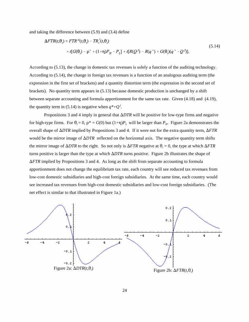
(5.13)

24

Figure 2a: )DTR(t,2i) Figure 2b: )FTR(t,2i)

and taking the difference between (5.9) and (3.4) define

(5.14)

According to (5.13), the change in domestic tax revenues is solely a function of the auditing technology.

According to (5.14), the change in foreign tax revenues is a function of an analogous auditing term (the

expression in the first set of brackets) and a quantity distortion term (the expression in the second set of

brackets). No quantity term appears in (5.13) because domestic production is unchanged by a shift

between separate accounting and formula apportionment for the same tax rate. Given (4.18) and (4.19),

the quantity term in (5.14) is negative when q*…Q f.

Propositions 3 and 4 imply in general that )DTR will be positive for low-type firms and negative

for high-type firms. For 2i = 0, D* = G(0) but (1+0)PL will be larger than PH. Figure 2a demonstrates the

overall shape of )DTR implied by Propositions 3 and 4. If it were not for the extra quantity term, )FTR

would be the mirror image of )DTR reflected on the horizontal axis. The negative quantity term shifts

the mirror image of )DTR to the right. So not only is )FTR negative at 2i = 0, the type at which )FTR

turns positive is larger than the type at which )DTR turns positive. Figure 2b illustrates the shape of

)FTR implied by Propositions 3 and 4. As long as the shift from separate accounting to formula

apportionment does not change the equilibrium tax rate, each country will see reduced tax revenues from

low-cost domestic subsidiaries and high-cost foreign subsidiaries. At the same time, each country would

see increased tax revenues from high-cost domestic subsidiaries and low-cost foreign subsidiaries. (The

net effect is similar to that illustrated in Figure 1a.)

25

5.2 Comparisons when separate accounting and formula apportionment induce different equilibrium tax

rates.

Separate accounting can also result in a different equilibrium tax rate than formula

apportionment, i.e. t s … t*. I will show there exists a value for F (reflecting the noise in the auditing

technology) for which equilibrium tax rates will be the same for both systems. As a benchmark, consider

the optimal tax rate when the two countries form a single tax area. With a single tax area, the countries

no longer need to deal with allocating taxable income. The optimal tax rate, which will maximize

, implies that . Denote this optimal tax rate by topt. The quantity produced

by multinational i in each country will equal . With formula apportionment,

implies t* < topt. The strategic distortion in the separate accounting case is harder to evaluate. First, the

sign of can be either positive or negative as in Sørenson (2003, 2004) and second, a single tax

area eliminates the need for auditing as long as countries use a non-discriminatory tax rate.

In the limit as the auditing technology perfectly reveals firm type, that is as F goes to 0, t s

converges to t opt. This means that for F sufficiently small, equilibrium tax revenues under separate

accounting will dominate those under formula apportionment. In the limit as F converges to 4, the signal

:j provides no information to update beliefs. In this case, the penalty range is independent of :j so each

type of firm will choose the highest or lowest possible transfer price that is not subject to a penalty (either

G(2+($)) or G(2-($))). The equilibrium tax rate under separate accounting will be much lower than t* and

tax revenues will be uniformly lower under separate accounting. Given the continuous structure of the

separate accounting game, there will exist a value for F such that equilibrium tax rates under separate

accounting and formula apportionment are equal. Denote this value by F*. This result is analogous to

results in Nielsen et al. (2002), Sørenson (2003,2004), and Kind et al (2005). Although the specific

structure of our models differ, in each paper there are a set of parameter values for which separate

accounting yields a higher symmetric equilibrium tax rate and other parameter values for which formula

apportionment yields the higher rate. What one can assess in this model, and not in the others, is how

equilibrium firm profit and equilibrium tax revenues differ by type.

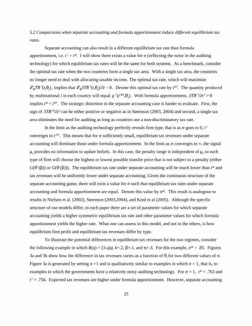
To illustrate the potential differences in equilibrium tax revenues for the two regimes, consider

the following example in which R(q) = (3-q)q, k=.2, $=.1, and 0=.3. For this example, F* . .85. Figures

3a and 3b show how the difference in tax revenues varies as a function of 2i for two different values of F.

Figure 3a is generated by setting F =1 and is qualitatively similar to examples in which F > 1, that is, to

examples in which the governments have a relatively noisy auditing technology. For F = 1, t* = .763 and

t s = .756. Expected tax revenues are higher under formula apportionment. However, separate accounting

26

-6 -4 -2 2 4 6

-0.0125

-0.01

-0.0075

-0.005

-0.0025

0.0025

Figure 3a: TR si - TR i for F = 1(implying t* > t s)

will generate more tax revenues than formula apportionment from high types and less from low types. As

F increases, the equilibrium tax rate and the equilibrium tax revenues under separate accounting decrease.

For example, with F = 1.5, ts = .6 and formula apportionment uniformly generates higher equilibrium tax

revenues.

Figure 3b is generated by setting F = .5. Now, ts = .77 and while separate accounting yields

higher expected tax revenues than formula apportionment, formula apportionment generates higher tax

revenues from high types and lower tax revenues from low types. The type-specific impact of the two

regimes has reversed itself.

-4 -2 2 4 6

-0.005

0.005

0.01

Figure 3b: TR si - TR i for F < 1 (implying t* < t s)

When the two systems generate different equilibrium tax rates, analyzing differences in domestic

vs. foreign tax revenues now requires that we look at

(5.15)

and

. (5.16)

Eqs. (5.15) and (5.16) differ from (5.13) and (5.14) by a common term that measures the difference in

formula apportionment tax revenues at t s and at t*. As long as t s is less than t* or t s is not too much

larger than t*, Proposition 2 tells us that this difference must either be strictly decreasing in t* for all 2i or

decreasing in t* for low values of 2i and increasing in t* for high values. For the example reported above

27

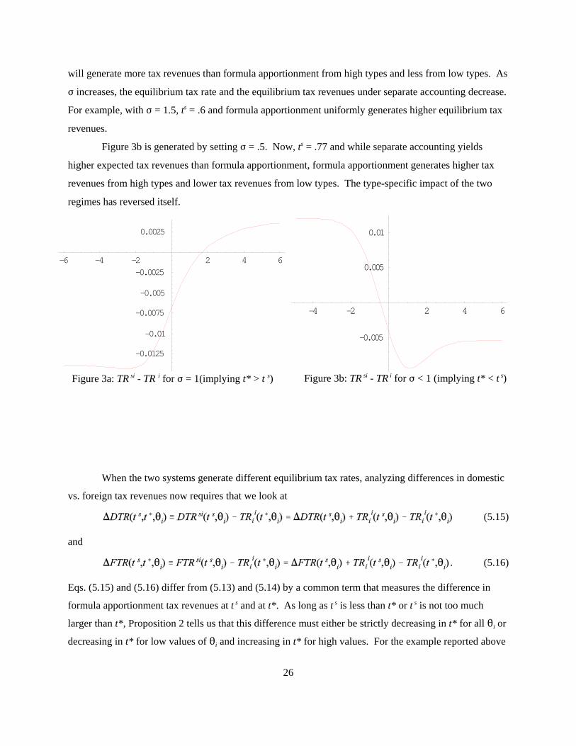
in which F = 1, the latter case arises and (5.15) is shown in Figure 4. Notice that an increase in the

equilibrium tax rate when moving to formula apportionment implies that each country will earn higher tax

revenues under formula apportionment from its lowest-cost domestic firms. This will be true regardless

of whether case (a) or case (b) from Proposition 2 arises. If case (b) arises, then each country may also

collect fewer tax revenues under formula apportionment from its highest-cost domestic firms. For a small

decrease in the equilibrium tax rate when moving to formula apportionment, the negative region in Figure

2a will arise for fewer types. The type representing the lower bound for this region will increase and the

upper bound (+4 in Figure 2a) may decrease. Regardless of the Proposition 2 case that arises, a shift to

formula apportionment that does not lower the equilibrium tax rate too much will generate a non-

monotonic relationship between firm type and the change in domestic tax revenues.

Proposition 8 (Domestic Tax Revenues).

i) If t s < t*, then there exist types *1 < * 2 < * 3 # 4 such that each country will earn higher tax revenues

under formula apportionment from its domestic firms if, and only if, 2i < * 1 or * 2 < 2 i < * 3.

ii) If t s is not too much larger than t*, then there exist types * 4 < * 5 # 4 such that each country will earn

higher tax revenues under formula apportionment from its domestic firms if, and only if,

* 4 < 2 i < * 5.

To assess tax revenue changes from foreign-owned subsidiaries first suppose t s < t*. If

Proposition 2a applies, the total change in foreign tax revenues is described by shifting )FTR down for

all 2i. This must increase the set of foreign subsidiary types that yield more tax revenue under formula

apportionment and will now include the highest-cost foreign subsidiaries. If Proposition 2b applies, the

left side of )FTR will shift down and the right side will shift up. Each country will still generate higher

tax revenues from some low-cost foreign subsidiaries but not from any of the highest-cost ones. Second,

suppose t s is a little larger than t*. If Proposition 2a applies, the total change in foreign tax revenues

corresponds to an upward shift in )FTR for all 2i. This shift decreases the set of foreign types that pay

more taxes under formula apportionment. If Proposition 2b applies, the left side of )FTR still shifts up

but the right side will shift down. Each country will now collect higher taxes from the highest-cost

foreign subsidiaries and will collect lower taxes from the lowest-cost foreign subsidiaries. Proposition 9

summarizes this analysis.

28

Figure 4: )DTR(t s=.756,t*=.763,2i)

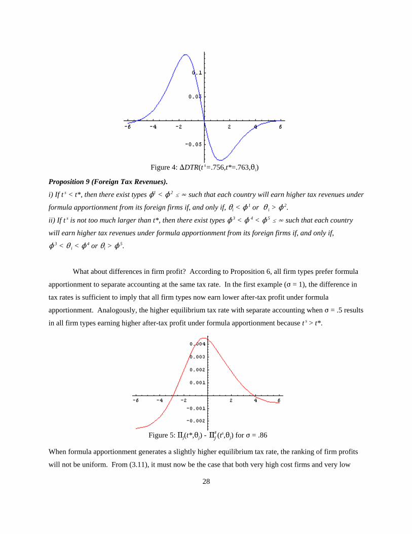
Figure 5: Aj(t*,2j) - (ts,2j) for F = .86

Proposition 9 (Foreign Tax Revenues).

i) If t s < t*, then there exist types N1 < N 2 # 4 such that each country will earn higher tax revenues under

formula apportionment from its foreign firms if, and only if, 2i < N 1 or 2 i > N 2.

ii) If t s is not too much larger than t*, then there exist types N 3 < N 4 < N 5 # 4 such that each country

will earn higher tax revenues under formula apportionment from its foreign firms if, and only if,

N 3 < 2 i < N 4 or 2i > N 5.

What about differences in firm profit? According to Proposition 6, all firm types prefer formula

apportionment to separate accounting at the same tax rate. In the first example (F = 1), the difference in

tax rates is sufficient to imply that all firm types now earn lower after-tax profit under formula

apportionment. Analogously, the higher equilibrium tax rate with separate accounting when F = .5 results

in all firm types earning higher after-tax profit under formula apportionment because t s > t*.

When formula apportionment generates a slightly higher equilibrium tax rate, the ranking of firm profits

will not be uniform. From (3.11), it must now be the case that both very high cost firms and very low

29

cost firms will earn higher profit with separate accounting. Figure 5 illustrates this phenomenon for

F = .86 which is greater than F*..85 and implies t s = .7626 while t* is still .763.

Proposition 10. Consider a small increase in F above F*. t s will be smaller than t* and there will exist

types : 1 < 0 < : 2 such that expected after-tax firm profit will be smaller under formula apportionment if,

and only if, 2i < : 1 or 2i > : 2. For F sufficiently large, expected after-tax firm profit will be smaller

under formula apportionment for all firm types.

Propositions 8 - 10 indicate the welfare implications of a shift from separate accounting to

formula apportionment is highly type dependent. When separate accounting supports a lower tax rate, the

only types that will earn higher profit, and from which the countries will see an increase in both domestic

and foreign tax revenues, fall between * 2 and N 1. When separate accounting supports a slightly higher

tax rate, this combination of higher firm profit and higher domestic and foreign tax revenues only comes

from types between *4 and N4. Both sets of types correspond roughly to the types near zero where )DTR

and )FTR are zero; two very small regions. In general, a shift to formula apportionment will generate

conflicts between domestic and foreign sources of tax revenues. The results also suggest the potential for

non-monotonic selection patterns if firms can choose between the two systems and tax rates differ across

countries. This latter issue however requires more careful examination. Finally, in terms of expected tax

revenues, the earlier examples associated with Figures 3a and 3b show that the regime with the higher tax

rate will generate higher expected tax revenue. This pattern is not general. For the linear example used

throughout this paper, formula apportionment yields higher tax revenues for all types when F=F*. Small

reductions in F will imply t s > t* but it will still be the case that formula apportionment will generate

higher expected tax revenues. Only with a sufficiently small F (as in Figure 3b) will separate accounting

yield a higher tax rate and higher expected tax revenues.

Finally, suppose one uses a transfer price standard consistent with short-run competitive prices

for intermediate good trade. Shifting to a compliance standard that requires the transfer price to reflect

sharing of foreign profits will introduce several competing incentives since the amount produced for the

foreign market affects a firm's compliance standard and its penalty regions. For fixed production

quantities, the new standard increases the penalty thresholds, :0 and :1. This change in :0 and :1 has an

ambiguous effect on whether a multinational engages in more or less profit-shifting and on its expected

unit penalty. An increase in :0 decreases the marginal penalty for overstating one's transfer price,

MPH/MDj, but has an ambiguous effect on the marginal penalty for understating one's transfer price, MPL/MDj.

30

If these changes in the penalty regions decrease PL +PH at the optimal transfer price, the firm will have an

incentive to increase foreign production but still produce less than the first-best amount.. Since an

increase in decreases :0 and :1, the increased production moderates the direct effect of the new

standard. However, if the changes in the penalty regions increase PL + PH at the optimal transfer price,

the firm will have an incentive to decrease foreign production which in turn increases :0 and :1. Now the

output response reinforces the direct effect of the new standard and increases the output distortions

associated with separate accounting. As a result, a shift to a stronger profit-shifting standard will not

change the qualitative results reflected in Propositions 8-10.

6. Conclusion

The problem of how best to apportion multinational profits between countries is inherently a

private information problem. Nonetheless, most of the literature comparing separate accounting and

formula apportionment either assumes complete information or assumes private information only in the

separate accounting analysis. To the best of my knowledge, this is the first paper to formally incorporate

private information in a positive comparison of both tax systems. In addition, I have introduced actual

compliance activity in the separate accounting model in the form of noisy auditing. The auditing

technology is structured to capture the idea that it is easier for a tax authority to detect income shifting

from firms with extreme types than it is from firms with more average types. (While government

compliance costs have not been modeled, the penalty functions do reflect some of the compliance costs

firms face. Any model in which overall compliance costs are proportional to g(A) will generate similar

results.) By focusing on the private information effects for both separate accounting and formula

apportionment, I can identify how a change from separate accounting to formula apportionment will

affect firm profit and tax revenues collected from domestic and foreign firms as a function of firm costs.

This analysis focused on the symmetric tax competition equilibria. This was done for two related

reasons. Symmetric equilibria allow one to focus on the marginal tax competition effects and for

comparison with the complete information literature which also focuses on symmetric equilibria. The

downside is that in equilibrium, there are no profit-shifting or production-shifting incentives. To have

either type of incentive persist in equilibrium would require asymmetries between countries or markets.

Small differences in either market revenues or country preferences would not alter the marginal tax

competition incentives significantly. They may however introduce level effects that could bias

performance towards either system. While the current paper does not incorporate market or country

asymmetries, it does provide a framework for investigating such effects.

Under the assumption that the symmetric tax rate is the same or higher under separate accounting

31

than formula apportionment, all firm types will earn higher after-tax profit under formula apportionment.

As the common tax rate under separate accounting falls below the common tax rate under formula

apportionment, then firm types in the tails of the type distribution will prefer separate accounting over

formula apportionment before types in the middle of the type distribution will. This is because the

auditing technology distorts the production decisions of the extreme types less than the production

decisions of middle types.

Tax revenues not only exhibit type-specific differences, they exhibit differences based on the

parent company's home country. Domestic tax revenues and foreign tax revenues are shown to respond to

a change from separate accounting to formula apportionment in very different ways. Moreover, the tax

revenue changes do not predict changes in firm profit. In fact, these results raise the interesting question

of whether letting firms self-select the type of tax system under which they will operate (as in Canada)

would generate adverse or positive screening effects for the countries. To arise in equilibrium, one would

need asymmetric countries to generate equilibrium differences in tax rates. We leave this important

question for future research.

Finally, it is important to comment on the manner in which private information has been

introduced in the model. In both the formula apportionment and separate accounting games, the

assumption that costs and quantities are observable technically means that both governments could infer

each firm's type. The reason such inference is not permitted in this paper is because one should think of

type as representing higher dimensional private information in which such inferences have already been

made. For example, suppose each firm made at least two input choices that are not observable by the

governments and also had private cost information. Observing total costs would allow each government

to infer the levels of the unobservable input levels if the firm's type was known. Without knowing firm

type, the best each government can do is reduce a multidimensional incomplete information problem

down to a one-dimensional problem. Gresik (2008) shows how this can be done and then uses the

inferred information to derive properties of optimal separate accounting and optimal formula

apportionment mechanisms. In the context of the current paper, the cost function can be interpreted as

already incorporating all of the indirect inference information about each firm's hidden type and hidden

actions. Another interesting extension of the current work would be to incorporate the hidden choice

information explicitly into the apportionment formula and then trace the equilibrium implications of using

a more sophisticated formula. One advantage of using the revenue formula in this paper is that it allowed

for an explicit derivation of tax competition effects, something that is not obtainable in the normative

analysis of Gresik (2008). The fact that many of the same non-monotonicities appear in both this paper

and in Gresik (2008) suggests that the observed patterns will be robust to the introduction of a more

32

complex information structure. Nonetheless, introducing multidimensional incomplete information into a

tax competition analysis represents yet another important direction for future research.

33

References

Anand, B. and R. Sansing, 2000, The weighting game: Formula apportionment as an instrument of public

policy. National Tax Journal 53: 183-200.

Baron, D. and D. Besanko, 1984, Regulation, asymmetric information, and auditing. RAND Journal of

Economics 15: 447-470.

Burbidge, J., K. Cuff, and J. Leach, 2006, Tax competition with heterogeneous firms. Journal of Public

Economics 90: 533-549.

Cremer, H. and F. Gahvari, 2000, Tax evasion, fiscal competition, and economic integration. European

Economic Review 44: 1633-1657.

Cremer, H., M. Marchand, and P. Pestieau, 1990, Evading, auditing, and taxing: The equity-compliance

tradeoff. Journal of Public Economics 43: 67-92.

Devereux, M., 2004, Debating proposed reforms of the taxation of corporate income in the European

Union. International Tax and Public Finance 11:71-89.

European Commission, 2002, Company taxation in the internal market, COM(2001) 582 Final, Brussels.

________ , 2005a, Code of conduct on transfer pricing documentation for associated enterprises in the

EU, COM(2005) 543 Final, Brussels.

________, 2005b, Tackling the corporation tax obstacles of small and medium-sized enterprises in the

Internal Market – outline of a possible Home State Taxation pilot scheme, COM (2005) 702, Brussels.

Gérard, M., 2005, Multijurisdictional firms and governments' strategies under alternative tax designs,

mimeo.

Gordon, R. and J. Wilson, 1986, An examination of multijurisdictional corporate income taxation under

formula apportionment. Econometrica 54: 1357-1374.

Gresik, T., 2008, Optimal Separate Accounting vs. Optimal Formula Apportionment, mimeo.

Hellerstein, W. and C. McLure Jr., 2004, The European Commission's report on company income

taxation: What the EU can learn from the experience of the US states. International Tax and Public

Finance 11: 199-220.

Kind, H., K. Midelfart, and G. Schjelderup, 2005, Corporate tax systems, multinational enterprises, and

economic integration. Journal of International Economics 65:507-521.

Mintz, J., 2004, Corporate tax harmonization in Europe: It’s all about compliance. International Tax and

Public Finance 11: 221-234.

Mintz, J. and J. Martens-Weiner, 2003, Exploring formula apportionment for the European Union.

International Tax and Public Finance 10: 695-711.

34

Mintz, J. and M. Smart, 2004, Income shifting, investment, and tax competition: theory and evidence

from provincial taxation in Canada. Journal of Public Economics 88: 1149-1168.

Nielsen, S., P. Raimondos-Møller, G. Schjelderup, 2002, Tax spillovers under separate accounting and

formula apportionment, mimeo.

_______, 2003, Formula apportionment and transfer pricing under oligopolistic competition. Journal of

Public Economic Theory 5: 417-436.

Multistate Tax Commission, 2003, State apportionment of corporate income.

http://www.taxadmin.org/fta/rate/corp_app.html.

Sørenson, P., 2003, Company tax reform in the European Union, EPRU working paper #03-08.

_______, 2004, Company tax reform in the European Union. International Tax and Public Finance 11:

91-115.

Zodrow, G., 2004, Tax competition and tax coordination in the European Union. International Tax and

Public Finance 11: 651-671.

35

Appendix

Proof of Lemma 1.

Recall that ,

, q*(t,2i) is defined by , and

.

a. TR i(t,2i) is decreasing in 2i.

Ai is clearly decreasing in 2i and .

b. If R) is concave, then is decreasing in 2i and TR i(t,2i) is strictly concave in t.

Direct calculation implies

.

Thus,

(A.1)

Using (3.9), (A.1) simplifies to

(A.2)

where . Standard comparative statics implies

which will be negative as long as R))) is negative (implied by concavity of R)). Therefore, (A.2) is

negative.

It is also the case that

. (A.3)

Since, , (A.3) simplifies down to

(A.4)

where

is negative when R) is concave. Hence, (A.4) is negative which means TR i(t,2i) is strictly concave in t.

c. Suppose is close to zero. If g)(2i) is negative, then TR i(t,2i) will be locally convex in

36

2i. If g)(2i) is sufficiently positive, then TR i(t,2i) will be locally concave in 2i.

With , differentiating twice with respect to 2i yields

(A.5)

Eq. (A.5) suggests that if q*(t,2i) is approximately linear in 2i, then the curvature of will be

inherited primarily from Ai(t,2i). From (3.10) we then know that for types at which g)(A) is negative,

equilibrium firm profit and equilibrium tax revenues must be locally convex. At types for which g)(A) is

sufficiently positive, equilibrium firm profit and equilibrium tax revenue will be locally concave.

This last result will be important for comparing tax revenues under formula apportionment and

separate accounting because it implies that marginal tax effects must fall into one of two cases. Recall

from (3.6) that . The concavity of TR i(t,2i) with respect to t and the fact that

implies that MTR i/Mt can depend on 2i in one of three ways:

i) There exists a such that for all , for all 2i;

ii) there exists a T > 0 such that for all t < T, for all 2i, and

iii) for each , there exists , such that for all , and

for all , .

The cutoff rates are defined so that and .

Proof of Proposition 2. Let t* denote a symmetric equilibrium of the Formula Apportionment game.

The proof involves showing that for any , for all 2i. Recall that

(A.6)

where it is understood that and . Differentiating the right-hand side of

(A.6) with respect to yields

37

(A.7)

and differentiating the right-hand side of (A.6) with respect to yields

. (A.8)

The bracketed term in (A.8) an be written as

. (A.9)

By concavity of the revenue function the first term in parentheses is less than one and by convexity of the

cost function, C(A,A,A), the second term is greater than one. Thus, (A.8) is negative, and so too is (A.7).

Completing the proof requires calculating and . Let Dkl denote the second

derivatives of firm i's direct profit with respect to (k or l equal to 1), (k or l equal to 2), and t j (l

equal to 3). Then,

(A.10)

and

. (A.11)

The denominators of (A.10) and (A.11) are positive and D11 and D22 are negative due to the standard

second-order conditions for profit maximization while D12 = -(1-t)C12 is positive. Next,

. (A.12)

By the same argument used to sign (A.8), (A.12) is strictly positive. Finally,

. (A.13)

With C12 equal to zero, is increasing in t j and is decreasing in t j.

Combining these signs with the signs of (A.7) and (A.8) implies that is strictly positive.

Because

, (A.14)

if , the left-hand side of (A.14) must be negative for all 2i while the second term on the right-hand

side of (A.14) must be positive for all 2i. Therefore the first term on the right-hand side of (A.14) must be

negative for all 2i. In order for t to be a symmetric equilibrium tax rate, (3.6) requires the expected value

38

of to be zero at t i = t. Thus, by contradiction, t must be no greater than .

Q.E.D.

Proof of Proposition 3.

a. At Dj = G(2j), (4.13) and (4.15) imply

(A.15)

and

(A.16)

Due to the symmetry of the normal distribution about the mean, (A.15) and (A.16) sum to zero when

2j = 0. For 2j > 0, each term in (A.15) is greater in magnitude than its counterpart in (A.16). Hence,

. Since profit-maximization implies that PH +PL is minimized, D*(2j) < G(2j). A

similar argument applied to the case when 2j < 0 implies D*(2j) > G(2j).

b. Let . Evaluating for at Dj=D*(2j) results in

(A.17)

By definition, the right-hand side of (A.17) equals zero when .

First, note that where M(A) is the standardized

normal distribution. For , this difference is positive and the first line of (A.17) is decreasing in .

Second, and are both positive. Since

E-1 is linear and increasing, the second and third lines of (A.17) represent the difference between two

strictly positive terms at any .

Suppose this difference is negative at and consider the marginal effect of increasing at

39

. The first line of (A.17) must be positive under this assumption. The only way this can be true is

if or . But this means

must be increasing in at . If is also greater

than , then will also be increasing in at but at a slower rate than

. In this case, the last two lines in (A.17) together must be decreasing in at

. Alternatively, if is less than , then is

decreasing in at . Now each line of (A.17) is decreasing in at . Therefore, when the

last two lines of (A.17) sum to a negative value, the right-hand side of (A.17) is strictly decreasing in

at . Thus, must be greater than for near 2j. Since 2j was chosen arbitrarily,

must be positive.

If instead this difference is positive, the first line of (A.17) must be negative. The only way this

can be true is if or . But this means

must be decreasing in at . If is also less

than 2j, then it too is decreasing in at but at a slower rate. Alternatively, if

is greater than 2j, then it is increasing in at . Both situations imply

that near , the last two lines of (A.17) are hence the entire expression is decreasing in . So

again, must be positive.

Finally, if one considers , similar arguments hold as well. Q.E.D.

Proof of Proposition 4.

To simplify the forthcoming expressions, let . By the Envelope Theorem,

. Since D*(A) is strictly increasing, is strictly negative at

D=D*(2j). For 2j > 0, this negative cross-partial implies that . For

2j < 0, this negative cross-partial implies that . To prove the desired result, we

will show that .

Note that

.

Changing the variable of integration in the second integral to -: implies that

. (A.18)

40

Since and since :<0 in (A.18), when 2j > 0 and

when 2j < 0. Consequently, . Q.E.D.

Proof of Proposition 5.

Consider the limit as 2j tends to +4. Clearly, PL goes to zero. Thus, we need to show that PH converges

to zero as well. From (4.13), note that for 2j sufficiently large,

. (A.19)

Alternatively,

. (A.20)

If one changes the first variable of integration in (A.20) to , then (A.20) can be written as

. (A.21)

As 2j goes to 4, F2j and both converge to 4. The integral in (A.21) thus converges to 1.

Since the first term in (A.21) can be no greater than 1, (A.21) converges to 0. Thus,

. But since PH must be non-negative, the limiting value must be zero. A similar

argument applies to the limit as 2j tends to -4. Q.E.D.