formation of cold gas filaments from colliding superbubbles · formation of cold gas filaments...
TRANSCRIPT

Formation of cold gas filaments
from colliding supershells
Evangelia Ntormousi


Formation of cold gas filaments
from colliding supershells
Ph.D Thesis at the faculty of physics
of the Ludwig–Maximilians–Universitat Munchen
Presented by Evangelia Ntormousi
from Thessaloniki, Greecein Munich, on February the 22nd, 2012


1st Evaluator: Prof. Dr. Andreas Burkert
2nd Evaluator: Prof. Dr. Harald Lesch


Contents
Contents vii
List of Figures x
Abstract xi
Zusammenfassung xiii
1 Preface 1
2 The Interstellar Medium 3
2.1 General . . . . . . . . . . . . . . . . . . . . . . . . . . . . . . . . . . . . . . . 3
2.2 Atomic Interstellar Gas . . . . . . . . . . . . . . . . . . . . . . . . . . . . . . 3
2.2.1 Molecular Interstellar Gas . . . . . . . . . . . . . . . . . . . . . . . . . 5
2.2.2 Ionized Interstellar Gas . . . . . . . . . . . . . . . . . . . . . . . . . . 7
2.3 Dust . . . . . . . . . . . . . . . . . . . . . . . . . . . . . . . . . . . . . . . . . 10
2.4 Cosmic Rays . . . . . . . . . . . . . . . . . . . . . . . . . . . . . . . . . . . . 11
2.5 Magnetic Fields . . . . . . . . . . . . . . . . . . . . . . . . . . . . . . . . . . . 14
2.6 The system as a whole . . . . . . . . . . . . . . . . . . . . . . . . . . . . . . . 15
2.6.1 Models of the multi-phase ISM . . . . . . . . . . . . . . . . . . . . . . 15
2.6.2 Cooling and Heating Processes of the Interstellar Gas . . . . . . . . . 16
2.6.3 The modern view of the ISM: the role of turbulence . . . . . . . . . . 21
3 Principles of Hydrodynamics 23
3.1 The equations of hydrodynamics . . . . . . . . . . . . . . . . . . . . . . . . . 23
3.1.1 The equation of continuity . . . . . . . . . . . . . . . . . . . . . . . . 23
3.1.2 The force equation . . . . . . . . . . . . . . . . . . . . . . . . . . . . . 24
3.1.3 The energy equation . . . . . . . . . . . . . . . . . . . . . . . . . . . . 25
3.2 Hydrodynamical Instabilities . . . . . . . . . . . . . . . . . . . . . . . . . . . 26
3.2.1 The Non-linear Thin Shell Instability . . . . . . . . . . . . . . . . . . 27
3.2.2 The Kelvin-Helmholtz Instability . . . . . . . . . . . . . . . . . . . . . 29
3.2.3 The Thermal Instability . . . . . . . . . . . . . . . . . . . . . . . . . . 32
3.3 The instabilities combined . . . . . . . . . . . . . . . . . . . . . . . . . . . . . 33
3.4 Some comments on turbulence . . . . . . . . . . . . . . . . . . . . . . . . . . 35
viii CONTENTS
4 Previous Work 39
4.1 Molecular Cloud Formation . . . . . . . . . . . . . . . . . . . . . . . . . . . . 394.2 Shell fragmentation and collapse . . . . . . . . . . . . . . . . . . . . . . . . . 41
5 Numerical Method 43
5.1 Solving the equations of hydrodynamics on a grid . . . . . . . . . . . . . . . . 435.2 The RAMSES code . . . . . . . . . . . . . . . . . . . . . . . . . . . . . . . . . 455.3 Sources and sinks of energy . . . . . . . . . . . . . . . . . . . . . . . . . . . . 46
5.3.1 Implementation of a new cooling and heating module . . . . . . . . . 465.3.2 Implementation of a winds . . . . . . . . . . . . . . . . . . . . . . . . 46
5.4 Creating turbulent initial conditions . . . . . . . . . . . . . . . . . . . . . . . 465.5 Simulation setup . . . . . . . . . . . . . . . . . . . . . . . . . . . . . . . . . . 48
6 Formation of cold filaments from colliding shells 49
6.1 Shell collision in a uniform diffuse medium . . . . . . . . . . . . . . . . . . . . 496.2 Shell collision in a turbulent diffuse medium . . . . . . . . . . . . . . . . . . . 56
7 Morphological features of the cold clumps 67
7.1 General . . . . . . . . . . . . . . . . . . . . . . . . . . . . . . . . . . . . . . . 677.2 Velocity dispersions . . . . . . . . . . . . . . . . . . . . . . . . . . . . . . . . . 747.3 Sizes . . . . . . . . . . . . . . . . . . . . . . . . . . . . . . . . . . . . . . . . . 747.4 Clump evolution . . . . . . . . . . . . . . . . . . . . . . . . . . . . . . . . . . 76
8 Metal enrichment of the clouds 79
8.1 Setup of the simulation . . . . . . . . . . . . . . . . . . . . . . . . . . . . . . 798.2 Metal enrichment of the gas from the OB associations . . . . . . . . . . . . . 848.3 Metal enrichment of the clumps . . . . . . . . . . . . . . . . . . . . . . . . . . 86
9 Summary and Conclusions 91
Bibliography 99
Acknowledgments 101
Curriculum Vitae 103

List of Figures
2.1 Distance calculation ambiguity . . . . . . . . . . . . . . . . . . . . . . . . . . 6
2.2 The ”Pipe” dark nebula . . . . . . . . . . . . . . . . . . . . . . . . . . . . . . 8
2.3 The ”Shamrock” nebula . . . . . . . . . . . . . . . . . . . . . . . . . . . . . . 10
2.4 Dense gas filaments . . . . . . . . . . . . . . . . . . . . . . . . . . . . . . . . . 12
2.5 The Milky Way in various wavelengths . . . . . . . . . . . . . . . . . . . . . . 13
2.6 Cooling-heating equilibrium curve . . . . . . . . . . . . . . . . . . . . . . . . 17
2.7 McKee & Ostriker (1977) view of the ISM . . . . . . . . . . . . . . . . . . . . 18
2.8 Cooling and heating rates of the local ISM . . . . . . . . . . . . . . . . . . . . 20
3.1 Illustration of the Vishniac instability. . . . . . . . . . . . . . . . . . . . . . . 30
3.2 Eddies created by the Kelvin-Helmholtz instability . . . . . . . . . . . . . . . 32
3.3 Instabilities in phase space . . . . . . . . . . . . . . . . . . . . . . . . . . . . . 34
3.4 Two-dimensional slab . . . . . . . . . . . . . . . . . . . . . . . . . . . . . . . 34
5.1 Energy and mass ejection from an ”average star” . . . . . . . . . . . . . . . . 47
6.1 Collision snapshots: uniform background . . . . . . . . . . . . . . . . . . . . . 50
6.2 Uniform background: zoom-in . . . . . . . . . . . . . . . . . . . . . . . . . . . 51
6.3 Gas phase histogram: uniform background . . . . . . . . . . . . . . . . . . . . 53
6.4 Gas fractions with time: uniform background . . . . . . . . . . . . . . . . . . 54
6.5 Number of clumps with time . . . . . . . . . . . . . . . . . . . . . . . . . . . 55
6.6 Collision snapshots: turbulent background . . . . . . . . . . . . . . . . . . . . 57
6.7 Turbulent background: zoom-in . . . . . . . . . . . . . . . . . . . . . . . . . . 58
6.8 Filament 1 . . . . . . . . . . . . . . . . . . . . . . . . . . . . . . . . . . . . . . 59
6.9 Filament 2 . . . . . . . . . . . . . . . . . . . . . . . . . . . . . . . . . . . . . . 60
6.10 Filament 3 . . . . . . . . . . . . . . . . . . . . . . . . . . . . . . . . . . . . . . 61
6.11 Filament evolution . . . . . . . . . . . . . . . . . . . . . . . . . . . . . . . . . 62
6.12 Phase histogram: turbulent background . . . . . . . . . . . . . . . . . . . . . 63
6.13 Gas fractions: turbulent background . . . . . . . . . . . . . . . . . . . . . . . 64
7.1 Condensing clouds . . . . . . . . . . . . . . . . . . . . . . . . . . . . . . . . . 68
7.2 Rotating clouds . . . . . . . . . . . . . . . . . . . . . . . . . . . . . . . . . . . 69
7.3 Clouds with random motions . . . . . . . . . . . . . . . . . . . . . . . . . . . 70
7.4 Clouds with low internal velocities . . . . . . . . . . . . . . . . . . . . . . . . 71

x LIST OF FIGURES
7.5 Cloud velocity dispersions . . . . . . . . . . . . . . . . . . . . . . . . . . . . . 727.6 Velocity dispersion with time . . . . . . . . . . . . . . . . . . . . . . . . . . . 737.7 Clump size distributions . . . . . . . . . . . . . . . . . . . . . . . . . . . . . . 757.8 Clump size over Jeans length distributions . . . . . . . . . . . . . . . . . . . . 757.9 Cores in the phase diagram . . . . . . . . . . . . . . . . . . . . . . . . . . . . 77
8.1 AMR-unigrid comparison . . . . . . . . . . . . . . . . . . . . . . . . . . . . . 808.2 Density and pressure histograms . . . . . . . . . . . . . . . . . . . . . . . . . 818.3 AMR-unigrid comparison: Mass fractions with time . . . . . . . . . . . . . . 828.4 Shell collision with metal advection . . . . . . . . . . . . . . . . . . . . . . . . 858.5 2d histograms: density-metallicity distribution . . . . . . . . . . . . . . . . . 878.6 Metal distribution of the clumps . . . . . . . . . . . . . . . . . . . . . . . . . 888.7 Metal content of the clumps with distance from the stars . . . . . . . . . . . 888.8 Metal content of the clumps with polar angle . . . . . . . . . . . . . . . . . . 89

Abstract
The aim of this work is to study the dynamics of the interstellar gas, with an eye towardsthe formation of the Cold Neutral Medium (CNM), gas with high densities (nH ≃ 100 cm−3)and low temperatures (T < 300 K). In particular, we want to explore the mechanisms thatcan lead to the filamentary structure typical of these clouds.
A natural mechanism for the formation of large amounts of cold gas in a small regionare converging flows. This type of problem has been studied extensively in the literature inthe form of academic, infinite high-Mach number flows that collide at a perturbed boundary.The novelty of our approach lies in simulating converging flows by using physically motivatedparameters, extracted from models of young stellar feedback. This feedback creates finite,structured shocks which are the seeds for turbulence at the shock collision interface.
In our numerical experiments two superbubbles, blown by the violent feedback of OBassociations, collide and fragment to form cold filaments through various fluid instabilities.The amount of cold gas formed, the morphologies and the kinematics of the cold gas clumpsare roughly in accordance with observed properties of such structures. In particular, oursimulations are able to capture the observed filamentary structure of the cold clouds andtheir fractal character.
The metal content of the clumps is tracked through an advected quantity in the code,inserted in the feedback regions along with the rest of the stellar feedback. Our studies showthat little or no enrichment happens from one stellar generation to the next, if only turbulentdiffusion is considered.
Although further work is needed in order to study the details of the clump structure andits dependence on the OB association parameters, this work opens a new path to the studyof the ISM dynamics by showing that complex characteristics of the observed structures canbe reproduced by applying physically motivated initial conditions.

xii LIST OF FIGURES

Zusammenfassung
Das Ziel dieser Arbeit ist es, die Dynamik des interstellaren Gases zu studieren, insbeson-dere die Entstehung des kalten neutralen Mediums, d.h. Gases mit hohen Dichten (nH ≃ 100cm−3) und niedrigen Temperaturen (T < 300 K). Wir wollen die Mechanismen, die die typ-ische filamentartige Struktur dieser Wolken erzeugen, im Detail verstehen.
Ein naturlicher Mechanismus fur die Entstehung großer Mengen kalten Gases in einemkleinen Gebiet sind konvergente Flusse. Diese Art von Problem wurde in Form von akademis-chen Flussen mit unendlich großen Mach Zahlen, die an einem gestorten Rand kollidieren,ausgiebig in der Literatur studiert. Unser Ansatz ist insofern neu, als das wir konvergierendeFlusse simulieren, indem wir physikalisch motivierte Parameter verwenden, die wir aus Mod-ellen fur das sogenannte Feedback junger Sterne erhalten, die aus Beobachtungen entstandensind. Dieses Feedback erzeugt endliche, strukturierte Schocks, die als Keime fuer Turbulenzenan den von kollidierenden Schocks erzeugten Grenzfluchen dienen.
In unseren numerischen Experimenten kollidieren zwei Superbubbles, erzeugt durch dasheftige Feedback von OB-Sternansammlungen, miteinander und fragmentieren, wobei sich aufGrund verschiedener, in Fluessigkeiten typischer, Instabilitaten kalte Filamente ausbilden.Die Menge an dabei geformtem, kaltem Gas sowie die Morphologie und Kinematik der soerzeugten kalten Gasklumpen stimmt in guter Naherung mit den fur derartige Strukturenbeobachteten Eigenschaften uberein. Insbesondere erwahnenswert ist, das unsere Simulatio-nen in der Lage sind, die beobachtete, filamentartige Struktur und den fraktalen Charakterder kalten Molekulwolken zu reproduzieren.
Innerhalb des Codes verfolgen wir die Metallizitat durch eine Große, die zusammen mitdem restlichen stellaren Feedback in der OB-Sternansammlung erzeugt wird, aber selbst keinespeziellen physikalischen Eigenschaften hat. Unsere Studien zeigen, das von einer stellarenGeneration zur nachsten, sofern nur die Ausbreitung durch Turbulenzen berucksichtigt wird,wenig oder gar keine Anreicherung mit Metallen erfolgt.
Obgleich zum Verstandnis der Details der Entstehung der klumpigen Strukturen undderen Abhngigkeit von den Parametern der OB-Sternansammlung weitere, detailiertere Stu-dien notig sind, offnet diese Arbeit jedoch neue Wege, die Dynamik des Interstellaren Mediumszu studieren, da sie beweist, das die komplexen Charakteristika der beobachteten Strukturendurch das Anwenden physikalisch motivierter Parameter in den Anfangsbediungungen repro-duziert werden konnen.

xiv LIST OF FIGURES

Chapter 1Preface
One Sun by Day, by Night ten thousand shineAnd light us deep into the Deity.
Edward Young, ”Night Thoughts”
In the late eighteenth century, Sir Frederick William Herschel came across a puzzling factin his deep sky observations: there were regions on the sky where there appeared to be nostars. This was not an easy observation to interpret. Did stars have a tendency to leavevoids in the Universe? As it so ofter happens in science, the explanation was as simple,elegant and exciting as it was surprising and unexpected. These celestial voids turned outto be ”dark clouds”, nebulae which obscure the background starlight almost entirely. Thisdiscovery revolutionized the way scientists view the cosmos, as it gave the first indication thatthe Galaxy contains non-stellar matter which fills the vast space between the stars.
Support for this interpretation actually came much later, from Johannes Hartmann’s(1904) discovery of an absorption line in stellar spectra that could only be explained byinterstellar absorption. Three decades later, in 1930, Robert Julius Trumpler showed that,apart from Herschel’s ”dark clouds”, interstellar space also contained a more diffuse gaseousmaterial, thus discovering one more of what we now know to be at least four gaseous phasesof Interstellar Matter. In the years that followed, the existence of all the other constituentsof the Interstellar Medium were discovered, dust, magnetic fields, and cosmic rays.
It is nowadays a known fact that the constituents of Interstellar Matter not only affect theway stellar radiation reaches the Earth, but they are also important ingredients of the Galaxyas a complex system, especially in due to their active role in the process of star formation.Interstellar gas is the building material for stars and it carries the energy and mass ejectedby them during their lives. Magnetic fields are thought to play an important role in theregulation of star formation. Dust, among others, provides an important cooling path for thegas and is an necessary catalyst for the formation of hydrogen molecules, as well as for otherchemical reactions.
As a complex system the Interstellar Medium makes a fascinating area of study on itsown, but it also holds great part of the solution to problems at much larger scales, as thelaboratory of Galactic evolution. At the time this text is written, the mystery of galaxyformation and evolution is yet to be solved. Although the ΛCDM model for dark matter has
2 CHAPTER 1. PREFACE
been very successful in reproducing the large-scale structure of the mass in the Universe, weare still far from understanding the mechanisms by which galaxies form their stars and thedetails of metal enrichment from one generation of stars to the next. Moreover, the processeswhich shape the distribution of masses in a young stellar cluster in an apparently universalway are still under debate and are possibly connected to the drivers of turbulence in theinterstellar gas.
I strongly believe the answers to all these questions lie on understanding the physics ofthe interstellar medium. However, this thesis does not aspire to answer them. Instead, itwould be considered successful by this author if it managed to break them down in simpler,more straightforward thought problems. More specifically, this is a thesis about the complexprocess of forming cold and dense gas out of the warm diffuse component of the interstellarmedium.
The novel ingredient in this work is that the hot energetic component of the interstellarmedium is controlling this transition, implemented in a self-consistent way, in the form ofwinds and supernova explosions from stellar models rather than as academic, perfect shocks.The non-linear nature of this system is what yields the complex cold structure we observe.Furthermore, this thesis studies the process of metal mixing between these components, withan eye towards the possible enrichment of the next generation of stars.
This counting as the first chapter of this work, the second chapter overviews the propertiesof interstellar matter as they are known at this time. The third chapter includes the theoreticalbackground needed to follow the phenomena studied in this thesis, essentially an overviewof hydrodynamics. The fourth chapter presents the current state of the art in the field ofcold cloud formation and hot shell expansion, thus giving a more detailed motivation for thiswork. The fifth chapter is dedicated to the description of the techniques used for the numericalmodeling of the systems under study, and the next chapters are dedicated to illustrating ourresults. The very last chapter summarizes and concludes the thesis.

Chapter 2The Interstellar Medium
2.1 General
Thanks to the continuous advances in astronomical observations it is now known that thespace between stars is not empty, but rather filled with gas, dust and energetic particles.
The different ways in which stars interact with this material, which is collectively called theInterstellar Medium (ISM), leave spectacular tracks for astronomers to follow : HII regions,reflection nebulae, luminous shocks and supernova remnants. By studying these fascinatingobjects it has been discovered, for example, that the matter which fills the space betweenstars is a mixture of hydrogen, helium and a small amount of heavier elements, in a gaseousor in a solid state.
Most of the solid state of the ISM is dust, an ingredient with very important effects on theradiation we receive from the ISM. The gaseous state itself comprises many phases, rangingfrom molecular, to cool atomic, to ionized gas. In this Chapter we give an overview of theknown properties of each of the gas phases, as well some general characteristics of interstellardust. We also briefly mention some features of the Galactic magnetic fields and cosmic rays,since they are important sources of pressure and also tracers of many physical processes inthe ISM.
2.2 Atomic Interstellar Gas
The phase of interstellar gas we refer to as neutral atomic gas is defined by the absence ofLyman continuum photons, meaning that hydrogen is mostly neutral. However, this termshould not be interpreted in a very strict sense, since other species can still be ionized in thismedium due to the dependence of interstellar extinction on wavelength. In fact, energeticcharged particles traveling in the Galaxy, known as cosmic rays, are known to cause partialionization even in the interiors of very dense clouds. What we call neutral atomic gas isactually not purely atomic, either. Some molecular lines have been detected in this medium,in the same way that atoms are known to exist in the coronas of molecular clouds.
The information contained in Chapter 2 is mostly a combination of material from the following sources:Tielens (2005), Lequeux (2005), Ferriere (2001) and Hollenbach & Thronson (1987), unless otherwise stated.Individual references for the information quoted here can be found in these reviews.

4 CHAPTER 2. THE INTERSTELLAR MEDIUM
There are several ways to study the neutral atomic ISM observationally, in emission andin absorption. Since interstellar gas is mostly hydrogen, we can study many of its propertiesby observing the well-known 21 cm line radio emission from this atom.
This line results from the hyperfine structure of the hydrogen atom, caused by the interac-tion of the magnetic moments of the electron and the proton within the atom. The transitionis strongly forbidden, with a spontaneous emission probability as low as Aul = 2.87×10⁻¹⁵s−1.Nonetheless, due to the enormous amounts of hydrogen in interstellar space we can indeedobserve it. It is usually detected in absorption in front of continuum radio sources or infront of 21 cm emission of warmer gas. Moreover, since the lifetime of the upper sublevel ismuch longer than the average collision timescale in ISM conditions, local thermodynamicalequilibrium (LTE) can be assumed for the gas when interpreting observations.
The main applications of 21 cm observations are to estimate the mass, the distributionand the kinematics of atomic hydrogen. From these observations we know, for example, thatatomic hydrogen amounts to at least half of the mass of the interstellar medium of our Galaxy.This is roughly true for most of the mass in other galaxies as well. Since the 21 cm line isusually assumed to be optically thin (meaning that we assume all the photons produced inthe emitting source can escape it), which might not always be the case, these masses aremostly upper limits.
By comparing absorption and emission spectra from the same region of the sky, we canidentify two phases of neutral atomic hydrogen. A dense (nH ≈ 10 − 50 cm−3), cold (T ≈100 − 300 K) phase, which is usually called the cold neutral medium (CNM), and a morediffuse (nH ≈ 0.1− 0.3 cm−3), warm (T ≈ 10000 K) phase, called the warm neutral medium(WNM). The WNM is extended in interstellar space and is mostly responsible for what weobserve in emission, while the CNM forms discrete, highly inhomogeneous and structuredfilaments, which appear in the spectra as absorption peaks. We should point out that thisextremely inhomogeneous structure of the CNM is believed to be a result of turbulence ininterstellar space, a process which is actually the main subject of this thesis.
The WNM contains as much mass as the CNM in our Galaxy, but it forms a thicker disk,with a scale height of |z| = 186 pc, compared to |z| = 106 pc of the CNM. From absoptionmeasurements we know that local cold clouds have a velocity dispersion of 6.9 km/sec andfrom emission measurements that the WNM has a velocity dispersion of about 9 km/sec.
The distribution of H I in the Galaxy can also be deduced from 21 cm observations,although not without some uncertainties. In general, it is very difficult to discern the exactdistribution of interstellar gas in the Galactic disk, the reason for this coming from theavailable ways to measure a cosmic object’s distance from us. For example, to measure thedistances to stars, when they are too far away to use parallaxes, we can use the differencebetween their apparent (m) and their absolute magnitude (M):
m−M = 5 logd
10pc−A (2.1)
where A is the extinction at the observed wavelength, primarily caused by interstellar dust.For the gas, however, it is not possible to measure distances this way, unless we know fromthe nature of the process that it is intrinsically spatially connected to stars. Examples of suchobjects are H II regions, formed by young massive stars as they ionize their surroundings(–See Figure 2.3 and Section 2.2.2). Another way to measure the distance to an object, whichalso comes from equation 2.1, involves determining the distance of stars unobscured by thecloud. This is applicable to dark, neutral clouds (–See Figure 2.2).

2.2. ATOMIC INTERSTELLAR GAS 5
Of course, a spatial correlation between stars and a region of the ISM only happens for afew clouds. In absence of such a fortunate coincidence, the only way to determine the distanceto a Galactic gaseous source is through its line-of-sight velocity, induced from its emissionor absorption spectrum. In the case of atomic hydrogen velocity estimates come from 21 cmhydrogen line observations. By making 21 cm obsrvations for many different lines of sight andcorrelating the resulting velocities with a model for the Galaxy’s differential rotation curve,we can calculate the object’s position in the Galaxy. It should be mentioned here that inemission this line probes the CNM and the WNM together.
Figure 2.1 illustrates a problem intrinsic to this method. For observations of the innerGalaxy (regions closer to the center of the Galaxy than the Sun) this method gives twopossible distance estimates for a given object, yielding an uncertainty for the distribution ofatomic hydrogen in these regions. It is still possible, though, to calculate the surface densityof H I. So far it has been found to be constant up to a radius of about 4 kpc from the center ofthe Galaxy, and decreasing beyond this distance. The vertical structure of atomic hydrogenis also estimated to be roughly constant with radius.
The distance uncertainty does not exist for the outer Galaxy, where we can make exactdistance measurements from 21 cm observations. In that part of the Galaxy, we can discernthe spiral arm pattern of the Galactic disk. Until 2008, our Galaxy was thought to havefour spiral arms, named Perseus, Cygnus, Carina and Orion after the constellations wherethey were projected. However, high-resolution observations with the Spitzer telescope, gavesignificant indications that our Galaxy possesses a bar in the inner parts and only two spiralarms, like most observed barred galaxies (Churchwell et al., 2009). It is also known thatatomic hydrogen exists at radii of at least 30 kpc from the center of the Galaxy and hat theouter part of the gaseous Galactic disk is warped.
Another important observable of interstellar neutral gas are the fine-structure lines ofcertain atoms, such as C I, C II, N I, N II, O I, O II and O III, to name a few. Fine-structureinteractions are interactions between the orbital momentum of the electrons in an atom andtheir total spin and for these species, they are mostly found in the far-infrared. These linesare the main coolants of the atomic interstellar medium, as we will explain in Section 2.6.2.
Finally, we can infer the chemical composition of interstellar matter from absorption linesobserved in the spectra of stars. We can distinguish the lines coming from interstellar gasfrom the intrinsic stellar lines because they have a fixed wavelength, unlike the periodicallyDoppler-shifted lines from the star, and because they are much narrower. The abundance ofhydrogen, for example, is calculated by fitting a theoretical profile to the observed Lyα line.Once the hydrogen column density is known, the elemental abundances of heavier atoms areexpressed in terms of the hydrogen abundance. If the observed line comes from a specieswhich is expected to be mostly neutral in the atomic ISM, then the procedure is similar tothat for Lyα. If more than one ionization state of the element is observed, then the abundanceis determined by solving the ionization equilibrium for the observed species.
2.2.1 Molecular Interstellar Gas
Although by far the most abundant molecule in the Galaxy is H2, there are many moremolecules in the ISM (more than 100 known so far) some of them very complex. We canfind molecular emission or absorption due to electronic transitions, like in atoms, but alsodue to vibrational and rotational transitions, in the spectra of the ISM, of the envelopes ofasymptotic giant branch stars and of comets.

6 CHAPTER 2. THE INTERSTELLAR MEDIUM
Figure 2.1: Illustration of a line of sight towards the inner galaxy and through the Galactic disk. For a given lineof sight velocity, there are two possible distances. (Image Credit: Ferriere (2001))
Vibrational transitions of molecules come from stretching, bending and deformation modes.Each vibrational transition can be further decomposed into rotational transitions, so they ap-pear in spectra as ro-vibrational bands. The typical energies for vibrational transitions are ofthe order of a fraction of an eV so the bands are observable in the near-infrared. Rotationaltransitions, on the other hand, have energies of the order of meV and we can usually observethem in sub-mm to cm wavelengths.
Molecular electronic transitions are of the order of a few eV and are generally found in thefar-UV. The most important results from such measurements come from H2 emission observa-tions, owing, of course, to the high abundance of this molecule. The highest intensity lines canyield interstellar H2 abundances. Comparison of molecular to atomic hydrogen abundancesin many lines of sight has shown that, above a gas column density of about N(H I)≥ 1021
cm−2 interstellar gas is almost entirely molecular. This has important consequences for theo-retical models of the Galactic ISM where one needs to include some measure of the molecular

2.2. ATOMIC INTERSTELLAR GAS 7
component without explicitly modeling the chemistry of atomic to molecular phase transition.
Ultraviolet observations are possible in relatively diffuse environments, where interstellarextinction from dust is not significant. Nevertheless, most of the molecular gas in our Galaxyis located in large and dense structures, called molecular clouds. These clouds contain alot of dust due to their high densities, which makes UV observations impossible. This, incombination with the fact that H2, being a symmetric molecule, has no permanent momentof inertia and thus no permitted transitions in the radio regime, has led astronomers to seeklines from other molecules as tracers of the internal structure of dense molecular clouds.
The next most abundant molecule in these clouds, which in addition has a rotationaltransition in the radio regime, is CO. Its J = 1 → 0 rotational transition at 2.6 mm can beused, in a similar way as the 21 cm line of H I, for mapping the large-scale distribution ofdense molecular gas in the Galaxy, since it is unaffected by dust extinction. Such surveyshave yielded a very high concentration of molecules in a region of 0.4 kpc radius around thecenter of the Galaxy, and a ring structure at radii between 3.5 and 7 kpc. It has also beenfound that molecular gas follows the Galactic spiral pattern very closely in the outer Galaxyand less dominantly so in the inner Galaxy, where the ring structure dominates (–see Figure2.5). Molecular gas is mostly confined at the midplane of the disk, with a scale height ofabout 81 pc.
High-resolution CO observations have shown that the mass distribution of molecularclouds is very hierarchical, with large structures containing ever smaller and denser cores.Hydrogen densities in these clouds range from 100 to 106 cm−3, organized in an almost frac-tal structure.
It is widely believed that molecular clouds are gravitationally bound, although there areuncertainties in what defines the limits of a cloud. In any case, that the vast majority ofobserved molecular clouds are in the process of gravitational collapse. In particular, it isthe dense cores within them that give birth to stars. After star formation has started in acloud, the remaining molecular gas is believed to be quickly photodissociated by the intenseradiation from the young stellar objects. The complex subject of star formation from densemolecular cores will not be treated in this thesis.
We will provide some more observational facts about molecular clouds in Chapter 4, andwe want to point out here that most of them are still derived from CO observations. Anotherway to get reliable mass estimates in the densest clouds is from dust extinction itself, a matterwe will explain further in Section 2.3, where we will discuss the properties of interstellar dust.
An important class of molecules in the ISM are Polycyclic Aromatic Hydrocarbons (PAHs).These are large molecules, the study of which is important, not only for understanding thechemistry of the ISM, but also for estimating its radiative heating and cooling rates, as we willsee in Section 2.6.2. These molecules are believed to be the origin of observed infrared bands.This emission is a fluoresence effect, in which a FUV photon absorbed by the molecule leadsto electronic excitations, with the energy re-emitted in the IR through vibrational modes ofthe molecule.
2.2.2 Ionized Interstellar Gas
The brightest stars in the Galaxy, O type stars, produce large amounts of high-energy photons,which are able to ionize hydrogen and helium around them. The energy required to ionizehydrogen is 13.6 eV, so photons with higher energies (UV wavelengths) will create a region ofionized hydrogen around the star. The remaining energy of photons which produced ionization

8 CHAPTER 2. THE INTERSTELLAR MEDIUM
Figure 2.2: An example of a darkcloud is the ”Pipe” nebula, named af-ter its elongated shape which resem-bles a smoking pipe. This nebula iscurrently not star-forming and it has afilamentary, self-similar structure typ-ical of molecular clouds. Located onthe sky in the constellation of Ophi-uchus, it is a small structure, of about5 pc in projected length. This im-age shows dust absorption overlayedon the background starlight. (ImageCredit: ESO/Yuri Beletsky)
is deposited in the free electrons of the plasma as thermal energy, effectively heating the gas.The ionized regions around O stars are called H II regions, after the fact that hydrogen inthese regions is fully ionized.
From their natural connection to very bright young stars we know that H II regions havethe same distribution as O-type stars in the Galactic disk, following the spiral density patternin the disk midplane and with a vertical scale height of about 80 pc.
The simplest description of an H II region, although not entirely accurate in most cases,is the Stromgen sphere. The Stromgen sphere is defined as a region inside which the numberof atom photoionizations by the stellar radiation per unit time is equal to the number ofrecombinations of the ions with free electrons. Since the absorption of UV photons by neutralhydrogen is very efficient, a Stromgen sphere has very well defined boundaries. Assuming auniform medium composed entirely by hydrogen, the radius of a Stromgen sphere is given by
RS = 30pc
(
N48
nHne
) 1
3
(2.2)
where N48 is the number of ionizing photons released by the star per unit time, in units of1048 s−1, nH is the neutral hydrogen number density and ne is the electron number density.
H II regions produce continuum radiation as well as line emission. The continuum is ther-mal Bremsstrahlung in radio wavelengths, produced by free electrons as they are deceleratedby the electric field of the ions. Thermal Brehmstrahlung can give us information on thetemperature of the plasma, which in this case is about 8000 K. Incidentally, the same valuecan be obtained by theoretical considerations, assuming that photoelectric heating balancesradiative cooling inside the ionized sphere surrounding the star. This gas is therefore called”Warm Ionized Medium”, to distinguish it from an even hotter phase we know exists in theISM.
In a wide range of wavelengths, free-bound continuum emission is also produced by therecombinations of free electrons with ions. This process gives rise to characteristic discontinu-ities , caused by recombinations to a hydrogen energy level. The less probable, but importantfor metastable atomic levels mechanism of two-photon radiative de-excitation also becomesimportant for H II regions, especially at wavelengths near 400 nm.
Naturally, we can also observe the permitted recombination lines of H, He and other

2.2. ATOMIC INTERSTELLAR GAS 9
elements from H II regions. These lines are very useful for determining dust extinction andelemental abundances of the ionized gas. Due to the low densities in these environments, wecan also observe forbidden lines if C, O and other species.
However, not all the ionized gas in the Galaxy is confined in H II regions. Indeed, wecan anticipate the existence of diffuse ionized gas in the interstellar medium by raising theassumption of a uniform medium surrounding the star, which enters the calculation of theStromgen radius. Since the position of the ionization front is inversely related to the gasdensity, if one side of the surrounding medium is slightly more rarefied, or if the surroundinggas is stratified in density (like the Galactic ISM along the vertical direction), we expect theionized gas to escape in the surrounding space in the direction of the less dense gas, extendingto distances larger than the Stromgen radius given by equation 2.2. This effect is called the”champagne effect”. Ionized gas from associations of young massive stars can also escape insurrounding space via the large cavities opened by the combination of their winds. It is notsurprising then that, although stars are created in the very dense environments of molecularclouds, ionized gas can be found up to relatively high Galactic altitudes.
The distribution of diffuse interstellar gas has been deduced by the scattering of pulsarsignals by the free electrons of the ionized gas, showing that this is actually the case. Theinteraction of the pulsar photons with the free electrons reduces the group velocity of the pulseproportionally to the wavelength. Then the spread in arrival times of different wavelengthswithin a pulsar signal will be proportional to the column density of free electrons along theline of sight to the pulsar. If we know the distance to the pulsar independently, we can deducethe number density of free electrons in the diffuse medium. With this method it has beenfound that the distribution of diffuse ionized gas in the Galaxy comprises a thin, annularcomponent at about 4 kpc from the center in the radial direction, probably connected to themolecular annulus at that distance and a more extended, thick disk, with a Gaussian scaleheight of at least 20 kpc. The average number density of this medium is of the order of 10−3
cm−3.In addition to the warm ionized gas, there is an even hotter ionized phase of the ISM,
usually referred to as the hot interstellar medium (HIM), with a temperature of about 106 K,which emits radiation in soft X-rays. This gas comes from supernova explosions when starsreach the end of their lives. It is also produced in large cavities, created by large stellar OBassociations. It is therefore always directly related to the star formation rate of a galaxy. Inthese regions, elements such as oxygen get collisionally ionized to give emission and absorptionlines of species such as O VI and O VII. Since interstellar X-ray observations probe emissionfrom distant hot gas superimposed with absoption from intervening clouds, it is difficult todiscetn the distribution of this hot gas in the Galaxy. We do know, however, that this gasreaches very high Galactic altitudes and that it occupies some 80-90% of the volume in theGalactic disk.
X-ray emitting gas, in particular O VI, has also been associated with structures in thehalo of the Galaxy called high-velocity clouds, which were first identified by 21 cm observa-tions. These clouds are moving with velocities of several tens of kilometers per hour and arebelieved to be falling into the potential well of our Galaxy. The X-ray gas connected to theseclouds could be coming from photoionization by a diffuse UV background, or it could be athermally unstable front between the cold gas contained in these clouds and an even hottergaseous halo, which could be detectable in soft X-rays in absorption. For a more detailedtreatment of this matter, which is outside the scope of this thesis, we refer the reader toNtormousi & Sommer-Larsen (2010) and references therein.

10 CHAPTER 2. THE INTERSTELLAR MEDIUM
Figure 2.3: The ”Shamrock nebula”,located at about 10 pc from the Sun,at the outer edge of our local spiralarm. It is a typical example of an HIIregion, where a central O type star il-luminates its parent cloud with strong,ionizing UV radiation. In this case thestar is CY Camelopardalis. The im-age is taken in the infrared band, atwavelengths of 12 and 22 µm, whichis emitted by the dust as it gets heatedby the central star. (Image Credit:NASA/JPL-Caltech/UCLA)
2.3 Dust
The importance of dust in the physics of the ISM and in the interpretation of astronomicalobservations in general cannot be overstated. Since dust is very well mixed with the interstel-lar gas, it is of extreme importance to understand its effects on the observed radiation andtake them into account both when analyzing observations and when producing theoreticalmodels of the ISM.
Dust is the main cause of the ISM opacities at wavelengths longer than the Lyman dis-continuity. It is also a cause of heavy metal depletion, since it keeps a large portion of thelocal ISM metals locked up in its grains. In addition, dust in a very important catalyst formany chemical reactions in the ISM. It provides not only a surface on which elements cancombine, but also a third body to receive the excess energy from certain chemical reactions.This is one of the reasons why in many regions the dust content is an indication of the gasmetallicity.
The alignment of elongated dust grains with the magnetic field of the Galaxy causes thelinear polarization of the radiation that passes through the ISM, giving us a means to observethe Galactic magnetic field.
The most straightforward way to observe dust in the Galaxy is by the reddening effectit has on background light sources. From equation 2.1 we know that the difference betweenthe absolute and the observed magnitude of a star depends on the dust extinction along theline of sight. By measuring the magnitude difference between a reddened star and a nearbystar of the same spectral type, which is unaffected by the intervening dust cloud, we cancalculate the color excess caused by the dust. Since stellar radiation covers a wide range ofwavelengths, from this process we obtain the color excess as a function of wavelength. The

2.4. COSMIC RAYS 11
resulting curve, called extinction curve, for the ISM shows an increase in extinction withincreasing wavelength. This is the reason why dust extinction is also called reddening.
By studying extinction curves we can derive the composition and sizes of interstellar dustgrains. For instance, the presence of a ”bump” in extinction curves in the UV, around 217nmindicates the presence of graphite particles. Infrared extinction bands, on the other hand,point to the presence of silicates. Absorption by dust is also a strong indicator of the totaldust volume, if the optical properties of the dust particles are known.
Dust absorbs FUV photons and re-emits them in the infrared. Most of the electronsexcited by the UV photons that hit the dust do not reach the surface of the grain. Theirenergy is left in the grain, which is thus heated and emits thermally in the infrared. Thisprocess has important implications for the heating and cooling of the ISM, as we will see inSection 2.6.2, but it also provides a means of observing the structure of the gas with spaceobservatories which are unaffected by the Earth’s atmosphere. A spectacular image of thestructure of the ISM as traced by dust emission in the infrared, as seen by the Herschelsatellite, is shown in Figure 2.4.
It follows from simple considerations of the way a solid particle can interact with electro-magnetic radiation, that the strongest interaction will happen for particles of similar size tothe incident wavelength. The fact that extinction curves depend on a wide range of wave-lengths indicates that interstellar dust particles have a distribution of sizes. Although theshape of the distribution of dust particle sizes is still debated, the grain radii are known tovary between about 0.005 and 1 µm.
Solid particles do not only absorb, they also scatter background light. Scattering is dom-inated by the largest dust grains and is what creates the ”reflection nebulae”, usually blue-colored reflections of starlight by a cloud containing dust.
Although the mechanisms by which dust can be destroyed are numerous, shocks andionizing photons being ubiquitous in the ISM and destructive for these particles, the originof dust in the ISM is still poorly understood. The standard picture of grain creation is fromplanetary nebulae and from cool stellar winds. In both cases, the temperature of the gasshould drop enough for the first nucleation to occur, namely for the bonds between particlesto switch from strong molecular to weaker, inter-molecular bonds. For this to happen, themetallicity of the gas should be high enough and its cooling rate should be fast. Afternucleation has begun, inter-particle collisions take over the growth of the grains. However,it is not clear if the production rate from these mechanisms is enough to account for allinterstellar dust, given the rate at which shocks ans supernovae can destroy it Salpeter (1977);Kochanek (2011); Draine (2011). On the other hand, the apparent element depletion insidedense molecular clouds could indicate that they are a site where dust could be forming.
2.4 Cosmic Rays
Mostly for historical reasons, we refer to energetic charged particles reaching the Earth fromspace as cosmic rays. These particles were initially thought to originate from the Earth itselfor from the atmosphere, until balloon experiments proved their extraterrestrial origin.
These particles are injected into the ISM by supernova explosions and by flares or coronalmass ejections from late-type stars. Actually, the lowest-energy cosmic rays that reach theEarth do come from the closest such star to the Earth, the Sun. Cosmic rays are accelerated tothe energies at which we observe them by turbulent magnetic fields and by crossing supernova

12 CHAPTER 2. THE INTERSTELLAR MEDIUM
Figure 2.4: Dense gas filaments in Polaris, as seen by the Herschel satellite at infrared wavelengths 250, 350 and500 µm,, coming from dust and PAHs.(Image credit:ESA/Herschel/SPIRE/Ph. Andre (CEA Saclay) and A. Abergel (IAS Orsay). )

2.4. COSMIC RAYS 13
Figure 2.5: A collection of images of the Milky Way in 10 different wavelength bands. From top to bottom: 1.
408 MHz radio continuum, mostly synchrotron emission as electrons move in the Galactic magnetic field. 2. 21cm atomic hydrogen emission. 3. 2.4-2.7 GHz radio continuum, tracing hot ionized gas through the synchrotronemission of free electrons. 4. J = 1 → 0 CO emission in the radio, tracing the Galactic molecular gas. 5.
Composite image of mid- and far-infrared, principal tracer of interstellar dust emission. 6. Mid-infrared, comingfrom Polycyclic Aromatic Hydrocarbons. 7. Composite near-infrared image, probing unobscured radiation fromcool star. 8. Optical light, where we can see the regions obscured by dust. 9. X-ray emitting hot gas. Cold cloudsappear as shadows in this image. 10. Gamma rays, produced by cosmic ray collisions with hydrogen atoms in theGalaxy and by the scattering of lower energy photons to higher energies as a result of collisions with cosmic rayelectrons. (Image and caption credit: NASA Multiwavelength Milky Way project (http://mwmw.gsfc.nasa.gov/)and references therein)

14 CHAPTER 2. THE INTERSTELLAR MEDIUM
or other types of shocks as they propagate in the Galaxy.
Given their observed constitution and energy distribution, we could say a typical cosmicray particle is a proton of energy about 1-10 GeV. Protons actually make up about 85 % ofthe cosmic ray particles, the rest being alpha particles and 3% heavier nuclei. Cosmic raysalso contain electrons, positrons and nuclei of elements such as Li, Be and B, which originatefrom their interaction with ISM particles. Cosmic ray energies range from 109 eV to values ashgh as 1020 eV, the latter termed ultra-high energy cosmic rays (UHECR). Their distributionroughly follows a broken power-law behavior, starting from a slope of -2.75, becoming steeper(slope=-3) after an energy of about 1015 eV and flatter again, with a slope of -2.5 after about1018 eV.
The flow of cosmic rays to the Earth, especially at low energies, is regulated by themagnetic field of the Sun. The solar wind carries a significant magnetic field, which can trapthese particles before they reach our atmosphere. This makes the exact shape of the cosmicray energy spectrum quite uncertain. Cosmic rays also follow the magnetic field of the Galaxy,which makes them interesting tracers for studying its morphology (–see also Section 2.5).
The most important role played by cosmic rays in the ISM is that they provide a sourceof pressure. They are also the main cause of ionization in very dense environments, such asmolecular clouds. The small degree of ionization they provide inside molecular clouds is ofextreme importance for the coupling of the gas to the magnetic field.
2.5 Magnetic Fields
Cosmic rays gyrate aroung the field lines of the Galactic magnetic field, emitting synchrotronradiation (– see Figure 2.5). This radiation is an important probe of the Galactic magneticfield, if certain assumptions are made for the cosmic ray number densities in the Galaxy. Fromsuch modeling we know that the Galactic field on the plane of the disk can be decomposedinto a structured component, following the spiral density wave pattern, and a turbulentcomponent, with random direction. In the vertical direction it forms two disks: a thin diskof scale height of about 150 pc, and a thick disk of scale height about 1500 pc.
Synchrotron emission interpretations are very uncertain since they depend on assumptionsof the cosmic ray number densities and of the magnetic field strength. An independentmeasure of the strength of the magnetic field that can be used in such estimates, at leastfor its component along the line of sight to the observer, is the Zeeman splitting of certainatomic levels. Zeeman splitting is the result of the interaction of the magnetic moment ofthe electrons in an atom with an external magnetic field. In the Galaxy this method canbe applied to the 21 cm hydrogen line (with some adjustments to account for insufficientresolution that we will not discuss here). This of course renders it biased towards the densestregions. From Zeeman splitting measurements we know that the Galactic magnetic field hasa typical strength of a few µG.
When a linearly polarized electromagnetic wave propagates through a magnetized plasma,its plane of rotation rotates by an angle which is proportional to the square of its wavelength.This phenomenon, called Faraday rotation, can also be used to probe the magnetic field ofthe Galaxy, although only in ionized regions.
The role played by magnetic fields in the physics of the ISM is, on large scales, to confineinterstellar matter by providing a net pressure that can balance the self-gravity of the gas. Italso traps cosmic ray particles in the Galaxy, which is an additional source of pressure.

2.6. THE SYSTEM AS A WHOLE 15
In smaller scales, magnetic fields regulate the expansion of supernovae and superbubbles,as well as the dynamics of individual clouds, since there is a sufficient degree of ionization inall ISM phases for magnetic fields to be coupled to the gas. Magnetic fields have also beenargued to support molecular clouds against gravitational collapse.
2.6 The system as a whole
In the previous Sections of this Chapter we introduced the observed properties of the differentconstituents of the Interstellar Medium seperately. This is mainly justified by their differentmanifestations in observations and by the different physical state of each. Nonetheless, it hasprobably become evident to the reader that the different phases of the ISM not only interactwith each other, but they also regulate the behavior of the Galaxy as a system.
Stars, especially massive ones, are the trigger of most of the processes in the ISM. Youngstars, especially of early types, expel large amounts of matter in very energetic winds. Theyalso provide large amounts of ionizing radiation, heating and ionizing the ISM around them.The ionization either leads to the formation of well-defined H II regions, or escapes to formthe diffuse ionized medium.
Supernova explosions inject energies of the order of 1051 ergs to the gas surrounding thestar. What is more, in large associations of O and B stars, the combination of the stellarwinds and supernova explosions creates enormous cavities of hot gas, which compress the gasaround them. Such shells, being subject to cooling from various processes that we will explainin the following Chapters of this thesis, can fragment to give cold gas. However, the violentpassage of such a shock from a clouldlet can instead evaporate it, or trigger it to collapsegravitationally and give new stars.
2.6.1 Models of the multi-phase ISM
The different phases of the atomic ISM seem to be in rough pressure equilibrium with eachother. This points to a fluid instability known as Thermal Instability (–see Section 3.2.3 for adetailed description of the instabilty), as a formation mechanism for the CNM and the WNMphases.
This instability happens when the heating-cooling rate equilibrium curve on the density-temperature plane of the gas shows wide plateaus, separated by steep steps. An example ofsuch an equilibrium curve is shown in Figure 2.6. This gives two stable equilibria on eitherside of an unstable equilibrium point, defined by a line of constant pressure, for instance, likethe one shown in Figure 2.6. The region above the curve is where cooling is stronger thanheating and the region below the curve is where heating is stronger than cooling. When gasis perturbed from the unstable equilibrium point to the region above the curve by, say, acompression, cooling drives it to cool and condense further, until is reaches equilibrium again,to the equilibrium point on the high density regime. An equivalent process happens to drivegas that has been perturbed to lower densities and drive it to the plateau on the low densityregime. Depending on the exact shape of the equilibrium curve and the positions of theplateaus the densities and temperatures of the two phases can be different. This mechanismfor the formation of phases of the ISM was proposed by Field (1965). However, we know thatthe ISM possesses at least one more gas phase, the hot component, which is very importantfor its dynamics, as well as for its enrichment in metals, but it is not included in this model.

16 CHAPTER 2. THE INTERSTELLAR MEDIUM
The inclusion of the third component in a dynamical model of the ISM was first proposedby McKee & Ostriker (1977). In their model, the ISM is composed of spherical clouds, eachof them composed of a cold neutral core and surrounded by two envelopes, a warm neutralmedium immediately outside the cold core and a warm ionized corona as the outer surface ofthe cloud. The cold clouds are assumed to have a very low filling factor, of about 0.02-0.04.Their ionized coronas have a filling factor of 0.2, while practically the whole volume of theISM, with filling factors of about 0.7-0.8, is composed by a hot dilute medium, created bysupernova explosions. In fact, supernova explosions regulate the behavior of the ISM in thismodel, compressing and sometimes evaporating the cold clouds. In their view of the ISM, thetotal mass of the gas is conserved and the phases are in pressure equilibrium. A schematicview of this model is shown in Figure 2.7.
Although this model significantly improved our understanding of the ISM physics, mainlyby introducting the hot component, we now know that the neutral clouds are far from spherical(Figure 2.2) and that the hot phase of the ISM actually has almost double the pressure of theother phases and is thus sometimes driven outside the Galactic disk. An improved model forthe ISM, where the cold clouds appear as ”blobby sheets” rather than spheres, was presentedby Heiles & Troland (2003), based on their observations.
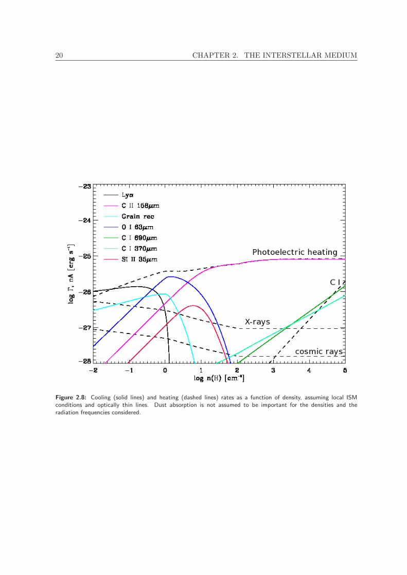
2.6.2 Cooling and Heating Processes of the Interstellar Gas
This Subection is in effect a summary of Wolfire et al. (1995). We refer the reader to thispaper for further details on the calculation of the rates.
One very important ingredient for understanding the formation of phases, by the mech-anism described briefly in the previous subsection, is the net cooling and heating of the gasas a function of its density and temperature. The combination of all possible cooling andheating paths of the gas will give an equilibrium curve like the one shown in Figure 2.6,which predicts the densities and temperatures of the different phases of the gas. Although wehave mentioned the possible heating and cooling mechanisms on the ISM in passing, here weexplain them in more detail, with a focus only on the atomic phase of the ISM. The heatingand cooling rates of the molecular phase, although of extreme importance for the study ofthe physics of molecular clouds, are outside the scope of this thesis.
Possibly the most important heating source of the atomic gas is photoelectric emissionfrom small dust grains and large molecules, such as PAHs. To remind the reader this well-known phenomenon, the photoelectric effect happens when a photon carrying an energy largerthan the work function of a material is absorbed by this material. Then it can give this energyto an internal electron, leading to the ejection of this electron. In the case of dust grains,the excess energy is mostly consumed in heating the grain, since most electrons liberated byUV photons do not reach the surface of the solid. However, for the 10% of electrons that doescape from the grain, the rest of the energy of the photon is available for heating the gas.The resulting heating rate from this process is
nΓphot = 10−24nǫG0 (2.3)
in ergs cm−3 sec−1. ǫ is the fraction of FUV photons absorbed by grains that is convertedto gas heating and G0 is the FUV flux in 1.6 × 10⁻³ ergs cm−2. Γphot is called the heatingfunction for this process and n is the number density of gas atoms.
ǫ is not a constant, but rather a function of temperature and electron density. It dependson the ionization rate divided by the rate at which electrons recombine on the surface of the

2.6. THE SYSTEM AS A WHOLE 17
Figure 2.6: Thermal instability mechanism. The cooling-heating equilibrium curve as a function of density andtemperature, assuming the cooling and heating rates described in the text, is plotted as a black curve and a straightline indicating a constant pressure curve is shown in orange. Gas parcels perturbed from the unstable regime A onthe curve towards higher densities will condense further until they reach the stable equilibrium C. In the same way,a volume of gas heated from A to higher temperatures or lower densities will continue heating and expanding untilit reaches equilibrium point B. We have then, the formation of two gas phases in temperatures and densities givenby points B and C.

18 CHAPTER 2. THE INTERSTELLAR MEDIUM
Figure 2.7: A schematic view of the ISM by McKee & Ostriker (1977). On the left (Fig. 1 of that paper), across-section of a typical cloud in their model. It is composed by a neutral atomic core, enveloped by a warmneutral and a warm ionized corona. The whole structure is immersed into the hot ionized medium.On the right (Fig. 2 of that paper),, a small-scale view of the passage of a supernova shock wave, coming fromthe upper right, from a region of the ISM filled with clouds such as the one shown on the left. A fraction of theseclouds will be evaporated.
grains. The maximum efficiency happens, of course, for low temperatures, when the grainsare mostly neutral.
The shape of the FUV spectrum has not been found to affect the resulting heating functiona lot, as long as the total flux remains constant. What does affect this heating rate appreciablyis, of course, the distribution of grain sizes. Usually, the distribution is assumed to be apower-law with a slope of about -3.5, based on models that take into account the observeddust emission.
The heating rate of the gas by photoelectric emission from dust and PAHs is shown inFigure 2.8 as the top dashed line. It is evidently the most important heating rate in the localISM. However, as we will explain shortly, under certain circumstances the photoelectric effectcan result in a net cooling of the gas.
Additional heating of the ISM comes from cosmic ray ionization of the gas and from diffuseX-ray radiation. Cosmic rays can ionize the gas to appreciable degrees, with an ionizationvalue usually adopted for the ISM being nζCR = 1.8× 10⁻¹⁷n cm−3 sec−1. After ionization,the excess energy is available for heating. Assuming a power-law distribution for the momentaof cosmic rays, which, as we have seen in Section 2.4, is a well-justified assumption, and takinginto account also secondary ionizations of H and He, the heating rate from this process is
nΓCR = nζCREh(E, ne/n) (2.4)
where Eh(E, ne/n) is the heat provided to the gas by each electron of energy E. This functiondepends on the electron fraction in the gas and the energy of the electron and is provided inthe Appendix of Wolfire et al. (1995).

2.6. THE SYSTEM AS A WHOLE 19
A similar process gives the heating rate of the gas from soft X-rays. Soft X-rays in theGalaxy are produced by energetic stellar feedback, mostly from young massive stars, althoughat the highest energies an extragalactic X-ray component dominates, coming mainly from ahot intergalactic medium. Without going into the specific details of the calculation, we quotehere the heating function calculated for this heating mechanism:
nΓXR = 4πn∑
i
∫
Jvhv
e−σvNwσivEh(E
i, ne/n)dv (2.5)
where the summation is assumed over all elements which experience primary ionization. Nw
is the column density of neutrals, hence the factor e−σvNw , which acconts for an absorbinglayer of neutral, warm interstellar gas, with the cross-section σv for absorption in frequencyv taking into account the elemental abundances. ne/n is the ionization fraction. Jv, theassumed X-ray flux spectrum, is calculated by including three X-ray components: A single-temperature component from nearby sources, a single-temperature component from largestdistances which has suffered absorption from interstellar clouds and an extragalactic power-law emission component. In Figure 2.8, heating from X-ray ionizations is the second mostimportant heating mechanism up to hydrogen number densities of about 103 cm−3, followedby cosmic ray ionization. At higher densities an important source of heating comes from thephotoionization of C I.
It has already been mentioned in earlier Sections of this Chapter that the most importantcoolants of the atomic ISM, especially in the low-temperature regime, are the fine structurelines of species such as O I and C II (–see Figure 2.8).
Important energy losses, mostly in the low-density regime, come from the recombinationof electrons onto small dust grains and PAH molecules, a process already mentioned whendiscussing heating mechanisms. When the thermal energy of the electrons that recombine onthe grains exceeds the energy of the electrons being ejected, then the net effect is an energy lossfrom the gas to the grains. It is clear that this effect is important at high temperatures, whenthe electron thermal energy, kT, is larger than the typical 1 eV carried by the photoelectricallyejected electrons. When modeling the gains and losses of the gas caused by the photoelectriceffect, the heating and cooling rates are calculated separately, so the net heating or coolingis defined as the difference between the two. The cooling by recombination of photoelectricelectrons is shown in Figure 2.8 as a solid black line.
In addition to the fine-structure lines, cooling can also happen due to emission in metastableor resonance lines. In particular, the collisional excitation of the Lyman α line can contributeto the energy losses of the gas in the highest temperature regime.
Figure 2.8 summarizes the cooling and heating processes that we have taken into accountin this work. In calculating these rates we have assumed that the lines are optically thin andthat dust extinction is not important. These assumptions are increasingly inaccurate as wemove towards the high density regime, but, since we are only interested in the transition fromwarm to cold gas, they provide an adequate description of the average cooling and heatingrates of the gas in this regime. The gas has been assumed to have a constant ionization degreein the calculation of the rates. The resulting cooling and heating curve for the parameters wehave used is shown in Figure 2.6. The abundances used in this calculation are roughly solar.
20 CHAPTER 2. THE INTERSTELLAR MEDIUM
Figure 2.8: Cooling (solid lines) and heating (dashed lines) rates as a function of density, assuming local ISMconditions and optically thin lines. Dust absorption is not assumed to be important for the densities and theradiation frequencies considered.

2.6. THE SYSTEM AS A WHOLE 21
2.6.3 The modern view of the ISM: the role of turbulence
As mentioned in Section 2.6.1, the inclusion of a third, hot phase of the ISM was proposedby McKee & Ostriker (1977) to account for cloud destruction and to count as a large volume-filling fluid. However, winds and supernova explosions from massive stars introduce a muchmore significant ingredient in the complex system of interactions in the ISM: they are a sourceof mechanical energy and, as such, the drivers of turbulence.
Turbulence, which will be treated in somewhat more detail in Section 3.4 as a consequenceof the equations of hydrodynamics, is a term to describe the coupling of different scales ofa fluid through the exchange of energy. It is characterized by a stochastic behavior andthe replacement of the local properties of a flow by statistical laws. In principle, one couldroughly describe a turbulent flow by the existence of curved shocks and eddies, appearing anddisappearing unpredictably, almost chaotically.
In this context it is therefore understood that a large-scale energy injection as violent as asupernova explosion or combined feedback from young OB stars will act as the beginning of anenergy cascade, creating smaller-scale eddies and shocks in the ISM. Although theoreticallysuch models have been proposed since a long time (ie de Avillez & Breitschwerdt (2004)),and the turbulent nature of all the phases of the ISM has been evident in observations foreven longer (Schneider & Elmegreen (1979); Lada et al. (1999); Hartmann (2002); Lada et al.(2007); Molinari et al. (2010), see also Figure 2.4 for a representative image of interstellarturbulence) it is very difficult to verify that the injection scale of interstellar turbulence hasa supernova origin.
Turbulence in the warm atomic phase of the ISM is thought to be roughly sonic (Verschuur,2004; Haud & Kalberla, 2007), meaning that the root mean square velocities of the gas areof the order of its sound speed (∼10 km/sec) while in the cold molecular phase it is thoughtto be supersonic, reaching velocities of 1-5 km/sec, while the sound speed in these clouds isroughly 0.2-0.5 km/sec (–see also Section 4.1 and references therein). This has importantimplications not only for global models of the Galactic ISM, but also for the star formationprocess, which happens exclusively in molecular clouds.
Interstellar turbulence is a very efficient mechanism for mixing newly-produced metalsfrom supernovae and stellar winds and dust in the gas. These elements can then participatein a new cycle of star formation. The velocity dispersion in the diffuse phase of the ISM hasa stabilizing role against the global gravitational instability of the Galaxy. Inside molecularclouds, the transition scale from supersonic to transonic or subsonic motions is probablewhat sets the scale of prestellar cores (Walch et al., 2011a), thus deciding the typical massof a protostellar object. It is therefore very useful to study the properties of interstellarturbulence and look for its drivers at different scales.
The fact that turbulence is maintained at the sonic level for the diffuse phase of the ISMis consistent with a picture in which the violent, evidently supersonic shocks from the drivers,possibly supernova explosions, distribute their energy to smaller scales through a cascade,until it is finally viscously dissipated. The root mean square velocity of such a flow can beproven to fall to sonic velocities very rapidly. The dissipation rate for sonic turbulence beingmuch slower, such a turbulent flow can be maintained for many crossing times, in this case,many Galactic rotation times.
However, the true puzzle in the studies of interstellar turbulence is what maintains thesupersonic velocities inside molecular clouds. Such supersonic motions should die out veryquickly, as we explained before, so there must be a process at molecular cloud scales which

22 CHAPTER 2. THE INTERSTELLAR MEDIUM
keeps driving turbulence in their interior. Star formation, through protostellar outflows hasbeen proposed as a possible driving mechanism. The formation scenarios of the clouds them-selves, however, very often invoke dynamical processes, which could also trigger turbulentmotions in the formed structures. This subject is analyzed addressed in detail in Section 4.1,as part of the motivation for this work; this thesis is partially aimed at explaining the originof turbulence in molecular clouds by proposing a very dynamical model for their formation.

Chapter 3Principles of Hydrodynamics
3.1 The equations of hydrodynamics
The work in this thesis can be essentially described as solving the equations of hydrodynamicsnumerically, for different boundary and initial conditions. It is therefore very important thatwe introduce these equations and some of their applications relevant to the phenomena wewill encounter in the following Chapters.
The equations of hydrodynamics provide a macroscopic description of the behavior ofa fluid. This means that the length and time scales of the system considered are muchlarger than those of the interactions between individual atoms or molecules. In practice, weare allowed to use this description of a fluid when the mean free path of the particles ismuch smaller than the size of the system under study. For all of the problems treated here,hydrodynamics is a more than sufficient approximation.
In hydrodynamics, the evolution of certain variables, representative of the state of the gas,is expressed as a function of space and time. In particular, we follow the velocity of the fluid,v(r,t) and any two thermodynamic quantities, usually the density ρ(r, t) and the pressurep(r, t), from which the rest of them, such as the temperature, can be derived.
In the following Sections the equations of hydrodynamics are derived from the conservationof mass, energy and momentum. We will refer to small volumes in the fluid as fluid elements.Again, these volumes may be considered infinitesimally small for the sake of the mathematicalderivation, but they are always large enough to contain a very large number of atoms ormolecules and the equations of hydrodynamics are always valid.
3.1.1 The equation of continuity
The first equation we are going to derive expresses the conservation of mass in the system.Considering a volume element dV of a larger volume V0 containing the fluid, the total massin the system can be expressed as
∫
ρ dV , where ρ is the density as a function of position andthe integral is taken over the volume V0.
Defining dn to be a vector with direction normal to the surface of the fluid element andmagnitude equal to the area of this surface, the mass flux through this surface per unit timeis equal to ρu · dn, where u is the fluid velocity vector. We consider dn to be positive in
The contents of Section 3.1 are from the first chapter of Landau & Lifshitz (1959)).

24 CHAPTER 3. PRINCIPLES OF HYDRODYNAMICS
the outward direction, so that the flux is positive when material is leaving the volume andnegative when material is entering the volume. Then the total flux of mass out of the volumeV0 is
∮
ρ u · dn (3.1)
where the integration is over the entire surface enclosing the volume V0. The mass flux outsidethe volume causes a decrease in the total mass contained in V0, which is equal to
−∂
∂t
∫
ρ dV (3.2)
By equating equations 3.1 and 3.2, we get
∮
ρ u · dn = −∂
∂t
∫
ρ dV (3.3)
and replacing∮
ρv · dn by its equivalent∫
∇(ρv)dV we get the equation of continuity
∂ρ
∂t+∇(ρ u) = 0 (3.4)
where the integral has been dropped, since this equality must hold for any volume in thefluid.
3.1.2 The force equation
The equation of force balance, in effect the equation of motion of the fluid, is also called theEuler equation, after L. Euler who derived it first.
Considering, as before, a volume element dV in a fluid of volume V0, we can express thetotal force acting on the fluid as the integral of the pressure over the surface enclosing thevolume:
−
∮
p dn = −
∫
∇ p dV (3.5)
By equating this force to the change in momentum of the fluid element, we get
ρdu
dt= −∇ p (3.6)
The derivative du/dt is here the total derivative of the velocity. This means that is carriesthe information on both the change of the velocity of the fluid in a given point in space aftera time dt, and the change in velocity experienced by the fluid element because it traveled adistance dr, to a different point of the fluid. To express this information explicitly, we canwrite
(
∂u
∂t
)
dt (3.7)
namely the change in velocity with time when the spatial coordinates, say x, y and z for aCartesian description, are held constant. Then the second part of the derivative, which is the

3.1. THE EQUATIONS OF HYDRODYNAMICS 25
part expressing the change in velocity due to the change in coordinates, can be written as
dx∂u
∂x+ dy
∂u
∂y+ dz
∂u
∂z(3.8)
which is equal to (du · ∇)u. So we have
du =
(
∂u
∂t
)
dt+ (du · ∇)u (3.9)
If we divide both sides by dt we can substitute this expression for the total derivative intoequation 3.6 and obtain:
∂u
∂t+ (u · ∇)u = −
1
ρ∇ p (3.10)
Equation 3.10 is the Euler equation. Additional terms are usually included in the right-handside of the equation to account for other forces that may be acting on the fluid, such asgravity.
Here the Euler equation was derived assuming that all the changes in pressure around thefluid element are consumed in changing its momentum. In other words, we have assumed noenergy losses due to viscosity or other dissipation mechanisms. This form of the equations ofhydrodynamics, when thermal conductivity and viscosity are considered to be negligible, iscalled ideal hydrodynamics and the fluids with these properties are called ideal fluids.
Assuming a negligible thermal conductivity is equivalent to saying there is no heat ex-change between different parts of the fluid. In other words, the motion of a fluid element isadiabatic. This condition can be expressed in terms of conservation of the entropy s of thefluid: ds/dt=0
∂s
∂t+ u · ∇ s = 0 (3.11)
which, in combination with the equation of continuity 3.4, gives an equivalent equation ofcontinuity for the entropy in the fluid:
∂s
∂t+∇(ρ s u) = 0 (3.12)
If we consider that, at some initial instant the fluid had the same entropy everywhere, equation3.12 becomes much simpler: s = constant.
3.1.3 The energy equation
The total energy of a fluid element, assumed to be fixed in space, can be expressed as
1
2ρv2 + ρ ǫ (3.13)
where ǫ is the internal energy per unit mass.
The change of the kinetic energy of the fluid with time can be written:
∂
∂t
(
1
2ρv2
)
=1
2v2
∂ρ
∂t+ ρ u
∂u
∂t(3.14)

26 CHAPTER 3. PRINCIPLES OF HYDRODYNAMICS
In equation 3.14 we can replace the first term of the right-hand side from the continuityequation, 3.4 and the second term from the Euler equation, 3.10. Then we obtain:
∂
∂t
(
1
2ρv2
)
= −1
2v2∇ (ρ u)− v · ∇ p− ρu · (u · ∇) u (3.15)
In equation 3.15 we can replace the term ρu · (u · ∇) u with 12 u · ∇ ∇2. If we define w as
the heat function per unit mass, then dw = Tds + V dp. By replacing V = 1/ρ, ∇ p can bewritten as ρ∇ w − ρT∇ s. Thus we get for the kinetic energy of the volume element:
∂
∂t
(
1
2ρv2
)
= −1
2u2∇ (ρ u)− ρ u · ∇
(
1
2u2 + w
)
+ ρTu · ∇ s (3.16)
The change in the internal energy of the fluid element with time, ∂(ρǫ)/∂t can be derivedfrom the first law of thermodynamics:
dǫ = Tds− pdV = Tds+p
ρ2dρ (3.17)
and, since ǫ+ p/ρ = ǫ+ p dV is just the heat function per unit mass w, we have
d(ρǫ) = ǫdρ+ ρdǫ = wdρ+ ρTds (3.18)
where we have also used V = 1/ρ and dV = −dρ/ρ2. So we can write for the change in theinternal energy of the fluid:
∂(ρǫ)
∂t= w
∂ρ
∂t+ ρT
∂s
∂t= −w ∇(ρ∇)− ρT u · ∇ s (3.19)
where equation 3.12 has been used to replace ∂s/∂t.
Combining equations 3.16 and 3.19 we get
∂
∂t
(
1
2ρu2 + ρǫ
)
= −
(
1
2u2 + w
)
∇(ρu)− ρu · ∇
(
1
2u2 + w
)
(3.20)
and finally∂
∂t
(
1
2ρu2 + ρǫ
)
= −∇
[
ρu
(
1
2u2 + w
)]
(3.21)
Equation 3.21 can be understood as the conservation of energy in each volume element as itmoves in the fluid, so that the energy carried by a fluid element is 1
2u2 + w.
3.2 Hydrodynamical Instabilities Related to Shell Fragmenta-
tion
An instability is defined in a physical system as the unbounded growth of initially smallperturbations imposed on an equilibrium state. Fluid instabilities are many times identifiedby the morphology of the system on which they are developing.
In the following Sections we will illustrate fluid instabilities relevant to the expansion andcollision of shock waves, such as the Non-linear Thin Shell Instability (NTSI), the Kelvin-Helmholtz Instability (KH) and the Thermal Instability (TI).

3.2. HYDRODYNAMICAL INSTABILITIES 27
We will not provide the full derivation of the perturbation equations or the solutions here,since such a lengthy analysis is outside the scope of this thesis. We will rather introduce themethodology and the assumptions that go into deriving the results, which are essential inorder to fully understand the results of our work, contained in the following Chapters. Therigorous derivations of the instabilities can be found in the references mentioned in the text.
3.2.1 The Non-linear Thin Shell Instability
This instability is very similar to the well-known Rayleigh-Taylor instability, which occurswhen a dense fluid is accelerated by a more rarefied fluid. In this case, however, the instabilityoccurs without the involvement of gravity, when the surface of a shock, bounded on one sideby thermal pressure and on the other by ram pressure, is perturbed by a ripple.
Let the spherical shock under consideration have an outer radius Rs and a thickness h,so that, the inner radius denoted by Ri, h = Rs − Ri. The shock is expanding with avelocity Vs in a uniform medium of density ρE and is driven by a medium of thermal pressurePi and negligible density (infinite sound speed). At this point we introduce the thin-shellapproximation, which significantly simplifies the derivation of the equations:
h
Rs< kh ≪ 1 (3.22)
∂
∂t≪
csh
(3.23)
where k is the wavenumber of the perturbation. Condition 3.23 essentially says that we wantthe evolution of the perturbations to be much faster than the sound crossing time of the shockthinkness, so that the shell reacts quasi-statically to the perturbation.
The equations of hydrodynamics, namely the continuity equation 3.4 and the Euler equa-tion 3.10 have already been introduced in section 3.1. For convenience, though, instead of thedensity ρ, the velocities ux, uy and uz and the pressure P, in this analysis here the variablesused are the surface density σ, the radial shock velocity Vr and the tangential shock velocityVT:
σ =1
R2s
∫ Rs
Ri
ρr2dr (3.24)
Vr =1
σR2s
∫ Rs
Ri
ρr2urdr (3.25)
VT =1
σR2s
∫ Rs
Ri
ρr2utdr (3.26)
In the absense of perturbations VT vanishes.The shock boundary conditions are:
[ρu] = 0 (3.27)[
P + ρu2]
= 0 (3.28)[
u
(
1
2ρu2 +
γ
γ − 1P
)
+ F
]
= 0 (3.29)
The detailed derivation of the thin-shell instability, as well as the contents of Section 3.2.1, can be foundin Vishniac (1983).

28 CHAPTER 3. PRINCIPLES OF HYDRODYNAMICS
where u is now the fluid velocity relative to the shock, F is the radiative energy flux and thesquare brackets denote differences across the shock. For an adiabatic shock F = 0.
Following the definitions of the new variables, 3.24-3.26, that is, integrating the equationsof hydrodynamics 3.4 and 3.10 across the shock and applying the shock jump conditions3.27-3.29 as boundary conditions, the evolution equations for σ, Vr and Vt are obtained:
∂σ
∂t= −2
Vs
Rsσ + ρEVs − σ (∇T ·VT) (3.30)
∂Vr
∂t= −
1
σ(ρEVsVr − Pi) (3.31)
∂VT
∂t= −
ρEVs
σVT −
Vs
Rs
VT +Vs
σuT(Rs)ρE −
∫ Rs
Ri
(c2sr2∇Tρ)dr
σR2s
(3.32)
where ∇T stands for tangential derivatives, uT(Rs) is the tangential velocity of the fluid atthe shock surface, as imposed by the boundary conditions, and Vs is the velocity of the shocksurface. In the derivation of equation 3.30 one assumes there is no matter flux through theinner boundary, that is, all the matter swept up by the shock as it propagates stays on itssurface.
The first term of equation 3.30 just states the obvious fact that, if the mass in the shellremains the same, the surface density of the shell decreases as its radius increases. The secondterm is the increase in surface density caused by material the shock accretes as it propagatesin the surrounding medium. The last term describes the mass transfer on the shell due tobulk tangential motions.
Equation 3.31 describes the change of the radial velocity of the shell as a result of thepressure difference at its outer surface, namely the ram pressure of the surrounding mediumρEVsVr and at its inner surface, namely the thermal pressure Pi provided by the hot gasdriving the shock.
In deriving equation 3.32 and, in fact, for the rest of Vishniac’s analysis of this instability,the assumption is made that the shock velocity is equal to the radial velocity: Vs = Vr, mean-ing that the motion of the shock is dominated by its radial expansion and not by tangentialmotions within it. This stems from the quasi-static assumption 3.23 and simple dimensionalarguments.
Equation 3.32 is of particular interest for the study of this instability. The first term onthe right-hand side is similar to the second term of equation 3.30, expressing the decrease intangential motions by the accretion of material from the surrounding medium. The secondterm just states the decrease in the tangential velocity as the radius of the shock increases.The third term tells us that the accreted material can only be accelerated in the directionof the shock front motion. Using the shock jump conditions, at the same time replacing thepressure at the outer boundary of the shock with the ram pressure, the last term can berewritten and equation 3.32 reads:
∂VT
∂t= −
ρEVs
σVT −
Vs
Rs
VT −csσ∇Tσ −
Pi
σ∇TRs (3.33)
where essentially the last two terms of equation 3.32 have been replaced by a term expressingthe effects of gradients in the surface density and a term due to changes in the inner surfaceof the shock. It might seem surprising then, that this term contains Rs instead of Ri. Thedetailed derivation omitted here, this is justified by the fact that irregularities that come from

3.2. HYDRODYNAMICAL INSTABILITIES 29
variations in the shell thickness are of higher order than irregularities coming from the bulkmotion of the shock.
It can be additionally shown that, if the inner thermal pressure balances the outer rampressure almost exactly, the term with ∇σ in equation 3.33 can be omitted. Now we havetwo terms, one due to mass accretion and one due to the curvature of the shell, plus one term(the last one), which accelerates material into lagging regions of the shell.
The appearance of this term in the equations is what causes the instability, in an analysisthat we will not include in this thesis. Figure 3.1, however, illustrates how an instability mightoccur due to the presence of this term. The pressures acting on the two surfaces of the shellare of different nature. The inner surface is supported by the isotropic thermal pressure, butthe outer surface of the shock is supported by ram pressure, which always acts on a directionnormal to the surface. This means that, if there is a ripple on the surface of the shell, thethermal pressure will push material sideways on the ripples. The ram pressure cannot balancethis motion, since it has no component in that direction. The result will be, to first order, atangential force on the shock surface, which will depend on the angle of obliqueness and onthe internal pressure.
The derivation of the perturbation equations from this point is straightforward. Here wewill just mention that, for example, for an isothermal shock and for a perturbation expressedin the form of spherical harmonics, the shell will be unstable and fragment on scales 6.4 < l <3M2, where l the azimuthal mode of the perturbation and M the Mach number of the shockexpansion velocity relative to the internal sound speed of the shock. The smallest wavelengthsare defined by the ”thin-shell” assumption and the largest wavelengths, comparable to theshock radius, are stabilized by the bulk motion of the shock. Additional effects that canstabilize or destabilize the shock are magnetic fields and the consideration of the thickness ofthe shock. The growth rate of the unstable modes is roughly csk(k∆)1/2 where cs the soundspeed, k the wavenumber along the shock, and ∆ the amplitude of the initial perturbation.
We should also note that, although the analysis quoted here is for the linear regime, theeffects we are interested in when we study this problem numerically are related to the non-linear growth of this instability, when the perturbations affect the expansion of the shock andthe quasi-static approximation is no longer valid. That is why in this text we quote this typeof instability as the ”Non-linear Thin Shell instability”. However, the above analysis is usefulbecause it shows us why there is an instability in the first place and what its first-order effectsare, which offers useful insight in the problem of shell fragmentation. This instability will bediscussed further in the text, since it is very relevant to our results.
3.2.2 The Kelvin-Helmholtz Instability
In Section 3.2.1 it was shown that when a spherical shock expands in a uniform medium,ripples on its surface can cause tangential motions of the material in lagging regions. Thistype of shear motion can give rise to another well-studied dynamical instability, called theKelvin-Helmholtz instability.
The Kelvin-Helmholtz instability occurs when a stratified, heterogeneous fluid with thedifferent layers in relative motion is perturbed. Its morphological signature are characteristiceddies, like the ones shown in Figure 3.2. In this Section we are going to present resultsrelevant to the case of an inviscid fluid, ignoring for sake of brevity the (stabilizing) effects of
A rigorous derivation of the KH instability (Section 3.2.2) can be found in Chandrasekhar (1961).

30 CHAPTER 3. PRINCIPLES OF HYDRODYNAMICS
Figure 3.1: Illustration of the thin shell instability, fromVishniac (1983) (Figure 1 of that paper). The differentnature of the thermal and the ram pressure cause rippleson the surface of the shock to grow by tangential motionsof the material towards lagging regions.
surface tension and magnetic fields.Using Cartesian coordinates, let the equilibrium configuration be that of a stratified fluid
with density ρ0(z) a function of height z, and a streaming velocity along the x-direction,ux0(z) also a function of z. Then the hydrodynamic variables can be expressed as:
ρ = ρ0(z) + δρ
p = δp
ux = ux0(z) + δux (3.34)
uy = δuy
uz = δuz
Inserting the expressions 3.35 for the variables in the equation of continuity 3.4 and the Eulerequation 3.10 and neglecting second order terms yields:
ρ0∂δux∂t
+ ρ0ux0∂δux∂x
+ ρ0δuzdux0dz
= −∂δp
∂x(3.35)
ρ0∂δuy∂t
+ ρ0ux0∂δuy∂x
= −∂δp
∂y(3.36)
ρ0∂δuz∂t
+ ρ0ux0∂δuz∂x
= −∂δp
∂z− gδρ (3.37)
∂δρ
∂t+ ux0
∂δρ
∂x= −δuz
dρ
dz(3.38)
∂δux∂x
+∂δuy∂y
+∂δuz∂z
= 0 (3.39)
where a term due to a gravitational acceleration g = gz has been included in equation 3.37and equation 3.39 expresses the incompressibility of the perturbation.
Looking for perturbations of the form:
exp [i (kxx+ kyy + ωt)] (3.40)

3.2. HYDRODYNAMICAL INSTABILITIES 31
equations 3.35-3.39 become:
iρ0 (ω + kxux0) δux + ρ0dux0dz
δuz = −ikxδp (3.41)
iρ0 (ω + kxux0) δuy = −ikyδp (3.42)
iρ (ω + kxux0) δuz = −dδp
dz− gδρ (3.43)
i (kxδux + kyδuy) =dδuzdz
(3.44)
Now by multiplying equation 3.41 by−ikx and equation 3.42 by−iky and add the resultingequations, replacing at the same time k2 = k2x + k2y and making use of equation 3.44, oneobtains:
iρ0 (ω + kxux0)dδuzdz
+ iρ0kxdux0dz
δuz = k2δp (3.45)
and from equations 3.43 and 3.44:
iρ0(ω + kxux0)δuz = −dδp
dz− ig
dρ
dz(3.46)
By eliminating δp from equations 3.45 and 3.46 the following equation is obtained:
d
dz
[
ρ0(ω + kxux0)dδuzdz
− ρ0kxdux0dz
δuz
]
− k2ρ0(ω + kxux0)δuz = gk2dρ0dz
δuzω + kxux0
(3.47)
The condition for instability is derived by applying appropriate boundary conditions andconsidering the specific form of the equilibrium configuration, functions ρ0(z) and ux0(z).
The simplest assumption we can make for the equilibrium flow is that of essentially twofluids, one of density ρ1 and velocity ux1 and one of density ρ2 and velocity ux2, superimposedon each other at z=0. (A similar configuration is shown in Figure 3.2).
The boundary conditions at z=-d and z=d (for a system of total size 2d along the zdirection) are just that the vertical components of the fluid velocities vanish on those surfaces.Additionally, we should ask that the components of the fluid velocities normal to their contactsurface vanish. In other words, the assumption here is that the two fluids do not mix.Omitting the intervening algebra, we directly present the condition for instability (modesgrowing exponentially in time), in the absence of surface tension:
k >g(α1 − α2)
α1α2(ux1 − ux2)2(3.48)
where α1 = ρ1/(ρ1 + ρ2) and α2 = ρ2/(ρ1 + ρ2). Interestingly, relation 3.48 states that, ifone ignores gravity, all wavenumbers are unstable to the Kelvin-Helmholtz instability. Thegrowth rate of the instability, for a step function in the velocity, is k∆v, where k the unstablewavenumber and ∆v is the velocity difference between the two layers.

32 CHAPTER 3. PRINCIPLES OF HYDRODYNAMICS
Figure 3.2: Simulated KH instability. A perturbation on the contact layer between two fluids of different density,shown here in black and white color, moving along the horizontal direction relative to each other, grows to givecharacteristic eddies like the ones shown in this figure. This configuration is already in the nonlinear regime of theinstability growth. (Image from wikimedia.org)
3.2.3 The Thermal Instability
The Thermal Instability has already been presented in Section 2.6.1 in a qualitative way.Figure 2.6 provides a schematic illustration of how this instability works. Here we will givesome dimensional arguments of when the instability takes place and what its overall behavioris.
LetL(ρ, T ) = 0 (3.49)
define the heating-cooling equilibrium curve of the gas, where L(ρ, T ) represents the energygains minus the energy losses of the gas per unit mass per unit time.
A perturbation of density and temperature is introduced, such that some thermodynamicquantity A, the pressure for example, remains constant. Then the entropy of the gas willchange by an amount δS and the heating-cooling function L will change by an amount δL:
δL dt = −Td(δS) (3.50)
where changes are to be calculated with A constant. Then the criterion for instability is
(
∂L
∂S
)
A
> 0 (3.51)
in other words, there is an instability if the gain-loss function L is a monotonous function ofthe entropy, so that changes in the entropy due to perturbations always cause a response ofthe same sign from the heating-cooling function and the perturbation ccan grow. Assuming
The contents of Section 3.2.3, as well as a full derivation of the TI can be found in Field (1965).

3.3. THE INSTABILITIES COMBINED 33
an ideal gas, for an isochoric perturbation T dS = CV dT and for an isobaric perturbationT dS = CP dT . Then one obtains two criteria for the instability, an isochoric and an isobaricone:
(
∂L
∂S
)
ρ
< 0, (isochoric) (3.52)
(
∂L
∂S
)
P
=
(
∂L
∂T
)
ρ
−ρ0T0
(
∂L
∂ρ
)
T
< 0, (isobaric) (3.53)
Criterion 3.52 is in principle incompatible with the force equation, because isochoric temper-ature variations will cause changes in the density, which then cannot be assumed constant.Condensations can be shown to be dominated by the isobaric condensation, which is compat-ible with the force equation. This can also be derived by a more detailed treatment of theinstability.
Burkert & Lin (2000) showed that the growth rate of the thermal instability does notdepend on the size of the perturbation (ie the wavenumber), but is rather determined by thelocal cooling time. In particular, the growth of a perturbation is decided by the transitionfrom isobaric to isochoric cooling. This implicitly means that the smallest perturbations willgrow first. The smallest unstable scale, according to their analysis, is decided by thermalconduction. In the discussion of our results we will comment more on the role of thermalconduction and its meaning with respect to our findings.
3.3 The instabilities combined
In the context of shell fragmentation it is very useful to study the effects of all the aforemen-tioned instabilities simultaneously, since each of them will contribute to the dynamics of theformed phases, if any. We naturally expect, however, that each instability will be dominantin different regimes, according to the size of the shock and the general properties of the gas.
Heitsch et al. (2008a) explored precisely this subject, separating the phase space of thegas into different regimes. Figure 3.3 from their paper illustrates the result:
To visualize this result, in Figure 3.4 we plot contours of the gas temperature for anidealized setup, designed to study the fragmentation of a shock due to these three instabilities.In this setup, a very thin slab between two infinite, high-Mach flows is perturbed. This isexpected to trigger the NTSI and in turn, the TI and the KHI. The Figure shows the resultsof two-dimensional hydrodynamical simulations of this setup after the instabilities have hadsignificant time to develop. Shown on the left is the result of a Mach 1 flow and on the rightthe result of a Mach 3 flow. In accordance with previous findings, we see that different flowMach numbers lead to slightly different results: Although both shocks are fragmenting, theone on the left shows more clumpy structure, signature of the TI, while the shock on theright is more violently disturbed by the NTSI, as indicated by the large finger-like strucuresgrowing perpendicularly to the slab.

34 CHAPTER 3. PRINCIPLES OF HYDRODYNAMICS
Figure 3.3: Instability regimes in density and temperature space. The solid black line shows the cooling-heatingequilibrium curve. Cooling instability causes fragmentation in the regions with positive slope and gravity is importantin the regions with negative slope. Red hatching shows where dynamics (KHI, NTSI) dominates over cooling andblue hatching shows where the TI dominates dynamics. (Figure and caption from Heitsch et al. (2008a))
Figure 3.4: Simulations of a perturbed slab, bounded on each side by an infinite flow. On the left, a Mach 1 flow.On the right, a Mach 3 flow. The colors indicate different contour levels of the logarithm of temperature. Thephysical scale is of 44 pc at each direction.

3.4. SOME COMMENTS ON TURBULENCE 35
3.4 Some comments on turbulence
Considering now a non-ideal fluid, that is, a fluid the kinematic viscosity of which is not neg-ligible, and also assuming incompressibility of the fluid flow, the equations of hydrodynamics3.4 and 3.10 become:
∇ · u = 0 (3.54)
∂u
∂t+ u · ∇u = −∇ p+ ν∇2u (3.55)
where ν is the kinematic viscosity of the fluid. Equations 3.54 and 3.55 are usually referredto as the Navier-Stokes equations.
In principle, the Navier-Stokes equations, supplemented with appropriate boundary andinitial conditions, include all the information we need in order to predict the behavior of afluid flow. However, even from everyday life, we are aware of flows which behave in a highlyunpredictable manner, such as the smoke of a cigarette as it rises in the air, or the flow ofwater behind a boat. These are examples of flows where the pattern changes rapidly, showinga dynamical, almost chaotic behavior. These kind of flows are called turbulent flows.
The study of turbulence has puzzled theoretical and experimental physicists for centuries,for the obvious reason that, in most cases, there appears to be no way to predict the flowpatterns seen in experiments directly from the Navier-Stokes equations, even when we knowthe boundary and initial conditions with high accuracy. Fortunately, however, it is possibleto formulate hypotheses based on the experimental data and then, from equations 3.54 and3.55 derive laws that can help predict properties of the flows.
One very important parameter in the study of turbulent fluid flows is the Reynolds number.It is defined as
R =L V
ν(3.56)
where L and V are a characteristic length and a characteristic velocity of the system understudy, respectively. It can be shown that the Reynolds number is in fact the only cotnrolparameter for a self-similar, incompressible flow, that is, a flow with defined geometricalshape. A well-known example of such a flow, the flow behind a solid circular cylinder, hasbeen studied extensively both in experiments and in simulations. Such studies show that thetransition from a laminar (ordered) flow to a turbulent flow is only controlled by the Reynoldsnumber. As the Reynolds number increases, the flow gradually loses its symmetries, until iteventually becomes turbulent.
For high Reynolds numbers, when the fluid is well into the turbulent regime (a state usuallyreferred to as ”fully developed turbulence”) there are two well-established experimental laws:The two-thirds law and the law of finite energy dissipation.
The two-thirds law states that, in a turbulent flow of very high Reynolds number, the
mean square velocity increment,⟨
(δu(l))2⟩
between two points, seperated by a distance l,
behaves as the two-thirds power of the distance:⟨
(δu(l))2⟩
∝ l2/3 (3.57)
The contents of Section 3.4 can be found in Frisch (1996). The phrasing of the experimental laws andtheoretical hypotheses has been quoted almost word for word from that text for exactness.

36 CHAPTER 3. PRINCIPLES OF HYDRODYNAMICS
The law of finite energy dissipation says that, if in an experiment on turbulence all thecontrol parameters are kept the same and only the viscosity is varied, brought to the lowestvalue possible, then the energy dissipation per unit mass of the fluid, dE/dt, behaves in away consistent with a finite positive limit ǫ.
These two experimental laws have been included in the form of three hypotheses, in orderto derive the famous Kolmogorov (1941) theory for turbulence. This theory, in accordance towhat we explained above, can only predict some statistical aspects of the flow, under certainconditions. It is, however, the closest we have to a theoretical description of turbulence.
The first hypothesis is formed to reconcile the apparent inconsistency of the mechanismsthat generate turbulence with the flow symmetries. The scale-invariance typically observed inturbulent flows must also be reconciled with potential boundary effects. Then the hypothesisis made that, in the limit of infinite Reynolds number, all the possible symmetries of theNavier-Stokes equations, usually broken by the mechanisms producing the turbulent flow, arerestored in a statistical sense, at scales small compared to the integral scale and away fromthe boundaries.
The term ”integral scale” above defines the length scale on which the turbulence drivingmechanism operates. This, in the case of the flow past a cylinder, for example, would bethe diameter of the cylinder. According to the first hypothesis then, the scales for which theKolmogorov theory is valid are always smaller than the integral scale, so that we do not haveto worry about effects due to the distance from the turbulence driver or boundary effects ofthe fluid.
The second hypothesis is necessary in order to explicitly express the scale invarianceof turbulence. Since in principle there are infinite possibilities for the scaling exponent ofthe flow, giving rise to infinite similarity groups. Under the same assumptions as the firsthypothesis, the turbulent flow is self-similar, in other words it possesses a single scalingexponent h ∈ R such that
δu(r, λl) = λhδu(r, l)
The third and final hypothesis that goes into the Kolmogorov (1941) theory is that, underthe same assumptions as in the first hypothesis, the turbulent flow has a finite, non-vanishingmean rate of energy dissipation, ǫ per unit mass.
Using these hypotheses, Kolmogorov derived the first and only exact result obtained so farto describe a turbulent flow, his famous ”four-fifths law”. Defining the longitudinal structurefunction of order p as
Sp(l) ≡⟨(
δu‖(l))p⟩
(3.58)
we can now express this law: In the limit of infinite Reynolds number, the third-order longi-tudinal structure function of homogeneous isotropic turbulence, evaluated for length intervalsl small compared to the integral scale, is given in terms of the mean energy dissipation perunit mass, ǫ (assumed to be finite and non-vanishing) by
⟨(
δu‖(r, l)3)⟩
= −4
5ǫl (3.59)
Equation 3.59 is not only an exact, non-trivial result of the Navier-Stokes equations, but itcan also be shown to stand, to an order of magnitude approximation, also for compressibleflows.

3.4. SOME COMMENTS ON TURBULENCE 37
Using the self-similarity hypothesis and dimensional arguments, it can be shown thatKolmogorov’s four-fifths law implies a power-law energy power spectrum in Fourier space:
E(k) ∼ ǫ2/3k−5/3 (3.60)
Relation 3.60 is an important scaling law for turbulence and we will be using it in our simu-lations.
Another interesting result of dimensional analysis relates to the numerical resolution nec-essary for modelling a turbulent flow. Using the velocity u0 and the length l0 at the integralscale, the expression with dimensions of energy dissipation of unit mass is ǫ = u30/l0. Thedissipation scale of turbulence, expected to happen at the viscous scale from molecular in-
teractions, is η =(
ν3
ǫ
)1/4. Then the ratio of the integral scale to the dissipation scale will
bel0η
∼
(
ν3
l0u30
)−1/4
= R3/4,
a function of the Reynolds number. This means that, for example, in order to simulate a flowof Reynolds number, say, 10000, we need at least 1000 grid cells per integral scale.

38 CHAPTER 3. PRINCIPLES OF HYDRODYNAMICS

Chapter 4Previous Work
4.1 Molecular Cloud Formation
In the previous Chapters we introduced some general features of the ISM as they are knownfrom observations, as well as the basic theoretical background necessary to understand thegas physics relevant to the dynamics of the ISM. Here we give the motivation for the work inthis thesis, which focuses on the formation mechanisms of the CNM and potentially molecularclouds as well.
Due to its very high density, molecular gas amounts to only a small fraction of the volumeof the Galactic interstellar medium, but it dominates interstellar mass (Ferriere, 2001). Morespecifically, only 1-2% of the gas volume in the Galactic disk is in the molecular phase, butit makes up about 50% of the total gaseous mass.
In Chapter 2 we mentioned that this phase of the interstellar medium exists in galax-ies in highly irregular clouds, with very clumpy, almost fractal structure. The large-scalemorphology of these clouds is very filamentary, according to observations in different wave-lengths (Schneider & Elmegreen, 1979; Lada et al., 1999; Hartmann, 2002; Lada et al., 2007;Molinari et al., 2010), mainly capturing CO transitions and dust absorption or emission andthus probing slightly different gas temperatures and densities. The internal density distribu-tion of molecular clouds is extremely hierarchical, with large, diffuse structures hosting densecores. Molecular clouds, as well as the dense cores in their interior, show a mass distribu-tion that can be very well described by a power-law. For the masses of molecular clouds inour Galaxy the power-law index is about -1.7 (ie Parmentier (2011)), while for the prestellarcore mass function the slope is shallower, of about -1.3 (ie Alves et al. (2007)). This be-havior indicates a very dynamical nature of the interstellar molecular gas. Explaining thesemorphological features is the main driver of this work.
Nevertheless, maybe the most important fact about molecular clouds is that they arethe sites of all observed star formation. In fact, there is a very well-known correlation ofthe column density of molecular gas with the star formation rate of a galaxy at large scales
This chapter is largely an adaptation of the introduction section of Ntormousi et al. (2011).

40 CHAPTER 4. PREVIOUS WORK
(Wong & Blitz, 2002; Kennicutt et al., 2007). Evidently, they must become gravitationallyunstable at some stage of their evolution. On the other hand, a typical molecular cloud massis about 104−5 M⊙, with a typical temperature of 50 Kelvin, which makes its collapse timeunder its own gravitation very short. Any model aiming at explaining star formation shouldthen account for the fact that, not only will such a cloud give several stars of typical massesaround 1 M⊙, instead of a single, 104−5 M⊙ object, but it will form them at a gas-to-starsconversion efficiency of only a few percent (Zuckerman & Evans, 1974).
There are many ideas as to why this should be so. One possible solution is that these cloudsbe sustained by strong internal motions, which can provide a support against gravitationalcollapse in the form of an additional internal pressure. Luckily, this view is also supported bythe large non-thermal line widths typically observed in molecular clouds, which do indicateinternal supersonic turbulence (Falgarone & Phillips, 1990; Williams et al., 2000). Turbulenceis also an elegant mechanism to fragment the cloud in smaller clumps, which can decouplefrom the rest of the cloud and become gravitationally unstable to give lower mass objects(Larson, 1981; Padoan, 1995; Klessen, 2001).
The interpretation of the aforementioned properties of molecular clouds in combination isa very challenging task, but it can be somehow alleviated by seeking a common characteristicto them, one they could inherit from the cloud formation process. If we identify this com-mon quality as non-linearity, then a natural formation mechanism for molecular clouds is acombination of fluid instabilities (Burkert, 2006).
One general example of an environment that would seed a non-linear fluid evolution, and atthe same time could assemble the large amounts of gas necessary for the formation of molecularclouds are large-scale converging atomic flows, an idea proposed by Ballesteros-Paredes et al.(1999) and Hartmann et al. (2001) to explain the fact that stellar populations in local star-forming clouds have age spreads that are significantly smaller than the lateral crossing time ofthe cloud. Such flows could in principle be anything from expanding shells (Elmegreen & Lada,1977a; McCray & Kafatos, 1987a), to colliding shells (Nigra et al., 2008), or flows generatedby large-scale gravitational instabilities (Yang et al., 2007; Kim & Ostriker, 2002, 2006).
Pringle et al. (2001) proposed an alternative mechanism for molecular cloud formation byagglomeration of gas which is already molecular. Although the formation of large clouds fromsmaller, already molecular clumps is a possible scenario (Dobbs et al., 2011), there is still noobservational evidence for the existence of a large molecular gas reservoir in the ISM outsidegiant molecular clouds.
Heitsch et al. (2006, 2008a) studied the formation of cold and dense clumps between twoinfinite flows which collide on a perturbed interface. Their study showed that cold structurecan arise even from initially uniform flows if the conditions favor certain fluid instabilities,such as the Non-linear Thin shell instability (NTSI, Vishniac (1994)), the Thermal Instability(Field, 1965) and the Kelvin-Helmholtz instability. We will discuss each of them in detail inthe following chapter.
Vazquez-Semadeni et al. (2006, 2007) used colliding cylindrical flows of tens of parsecslength, adding random velocity perturbations to the average flow velocity. This allowed themto study star formation efficiencies and the fates of individual clouds.
These numerical experiments have investigated the mechanisms which lead to the conden-sation and cooling of atomic to molecular gas and which cause the complex structure of theresulting clouds, independent of the specific mechanism driving the flows. In a further im-provement of these models, in this work we study the possibility for cold structure formationfrom colliding flows of limited thickness. Specifically, we model the expansion and collision of

4.2. SHELL FRAGMENTATION AND COLLAPSE 41
thin shells, created by wind- and supernova-blown superbubbles numerically and study theformed structures.
4.2 Shell fragmentation and collapse
Stellar feedback is a very powerful source of thermal and turbulent energy in the InterstellarMedium (ISM). Young massive stars, namely stars of O and B spectral types, produce ionizingphotons, expel large amounts of mass in winds and end their lives in supernova explosions, allprocesses which shape the matter around them in shells and cavities. Young OB associations,as groups of between 10 and 100 such stars are commonly called, will create giant shell-likeshocks in their surrounding space from the combined effect of their member stars. Such shellshave been repeatedly observed in our Galaxy in various wavelengths (Heiles, 1979, 1984;Ehlerova & Palous, 2005; Churchwell et al., 2006).
These shells are potentially unstable to non-radial perturbations as they expand, as shownby various analytic studies of thin, shock-bounded or pressure-bounded slabs (Vishniac,1994; Vishniac & Ryu, 1989). Vishniac’s analytical work on shell fragmentation has beenbriefly presented in section 3.2.1. On the other hand, perturbations on large, self-gravitatingshells are able to grow to the point where they can collapse to form stars (Elmegreen,1994; Whitworth et al., 1994), a scenario usually referred to as the ”collect-and-collapse”model. This process has been proposed as a trigger of star formation in many environments(Elmegreen & Lada, 1977b; McCray & Kafatos, 1987b).
An extensive numerical study of the instability of expanding shells, taking into accountnonlinear effects and the different parameters entering the shell expansion was presented in aseries of papers by Dale et al. (2009), Wunsch et al. (2010) and Dale et al. (2011). The focusof that work being only the gravitational instability of the shells, it is interesting to carryout an analysis of shell fragmentation due other instabilities, such as the Non-linear ThinShell Instability (Vishniac, 1983) for comparison. This is one of the numerical experimentscontained in this thesis.
Giant shells are expected to collide with each other as neighboring stellar associationsevolve (de Avillez & Breitschwerdt, 2004; Nigra et al., 2008), but whether or not these colli-sions happen before or after the shell has had time to fragment and gravitationally collapse isnot clear. If the shells were to collide before star formation had occurred on their surface, thecollision could trigger a phase change from the atomic gas gathered by the shocks to molec-ular gas, thus forming molecular clouds by the mechanism described briefly in the previousSection. The detailed processes which lead to this phase transition will become clearer in thefollowing Chapter.

42 CHAPTER 4. PREVIOUS WORK

Chapter 5Numerical Method
5.1 Solving the equations of hydrodynamics on a grid
In order to solve the equations of hydrodynamics numerically, they need to be discretized inspace and in time. There are various approaches to this problem, depending on the choice ofthe form of the equations and on the details of the numerical integration scheme. Here wewill briefly discuss the Eulerian class of methods because it contains the algorithm we haveused in our work. Eulerian methods discretize space on a mesh, usually Cartesian, and followthe evolution of fluid variables on the fixed locations of the grid points.
In principle, this class of methods first calculates the spatial derivatives that appear inthe equations of hydrodynamics, treating them at the right-hand side of the equations, andthen advances these quantities in time by a discrete step dt, treating the temporal derivativesas the left-hand side f the equations.
It is easy to understand that, when studying the propagation of a fluid on a grid, there isa point in the calculation at which the flux of material across the grid cell surfaces needs to becalculated. This is how the advection terms can be approximated in the grid configuration.The foundation for the class of methods we are going to be discussing here is the so called”Riemann problem”.
The Riemann problem is defined for an initial state of the fluid where all the variablesare strictly constant for, say, positive x and strictly constant for negative x, but their valueschange at x = 0: qi = qL for x < 0 and qi = qR for x > 0, where qi represent each of thehydrodynamic variables. It is now obvious how this problem relates to solving the equationsof hydrodynamics on a grid; at the smallest scales, each grid cell contains a state of the fluidwhich is constant across its length. The neighboring grid cell will, in principle, contain adifferent (constant) state of the fluid and the Riemann problem is perfectly defined at theirboundary.
In order to solve the Riemann problem for hydrodynamics, one needs to rewrite the
The short introduction to the Riemann problem contained in Section 5.1 is from ”Finite Volume Methodsfor Hyperbolic Problems” by Randall LeVeque.

44 CHAPTER 5. NUMERICAL METHOD
equations 3.4, 3.10 and 3.21 in a matrix form:
∂
∂t
ρuxe
+
ux ρ 01ρ
(
c2 − Pρ Γ
)
ux Γ
0 Pρ ux
∂
∂x
ρuxe
= 0 (5.1)
where we have written the equations only for one component of the velocity, ux, e is the totalenergy per unit mass of the fluid element, Γ = ρ
(
∂∂e
)
ρis called the ”Gruneisen exponent”
and c2 =(
∂P∂ρ
)
e+ P
ρ2
(
∂P∂e
)
ρis the sound speed. This form of the equations makes it a lot
easier to search for the eigenvectors of the system.
From a calculation we will omit here we get three eigenvectors, each representing a quantitycalled a ”Riemann invariant”. A numerical solver will have to calculate these quantities atthe cell interfaces. The solution can be pictured as waves propagating in the fluid containedin a grid cell. One class of waves contains the information for the propagation of the fluiditself and two are sound waves, one moving in the positive and one in the negative x-direction.The discrete step for advancing the equations in time will be decided on the condition thatthese waves not have time to cross the cell length in one timestep.
This is actually the basis for a numerical method called the Godunov method. In thismethod, a grid is defined by the centers of its cells. If we imagine that the x-direction hasbeen discretized, then the state of the gas qni at time step tn is known at the locations xi, thecenters of N intervals on the one-dimensional space we are considering. The cell interfacesare then xi+1/2, each between xi and xi+1. The Riemann problem can be solved at each oneof these intervals to give the transition of the fluid from one cell to the next. The time stepfor the numerical code will be chosen such that solutions from neighboring cells not overlap:
∆t ≤ min(∆ti) (5.2)
where
∆ti =xi+1/2 − xi−1/2
max(λi−1/2,k+)−min(λi+1/2,k−)(5.3)
and λi−1/2,k+ denotes the maximum positive eigenvalue of the matrix in equation 5.1 atinterface xi−1/2 and λi+1/2,k− the most negative eigenvalue at interface xi+1/2. This criterionis essentially a mathematical expression for what we described in words above: The timestepshould be smaller than the time it takes the fastest waves to cross a cell length, so that thesolutions do not overlap.
In Godunov schemes, in short, the solution advanced in time at position xi from time steptn to tn+1 is given by
qn+1i = qni +∆t
Fni+1/2 − Fn
i−1/2
xi+1/2 − xi−1/2(5.4)
where Fni+1/2 and Fn
i−1/2 are the fluxes calculated at the cell interfaces by solving the Riemannproblem.
For the numerical simulations in this work we have used the publicly available RAMSEScode (Teyssier, 2002), a Eulerian Cartesian code using a Godunov scheme to solve the equa-tions of hydrodynamics. The code has Adaptive Mesh Refinement (AMR) capabilities, ofwhich we have made use in some of the simulations in this thesis and which we will shortly

5.2. THE RAMSES CODE 45
discuss in the following Section. We will introduce the general features of the code, as pre-sented by its author, as well as adaptations we have made to selected modules to simulatephysics specific to our purpose.
5.2 The RAMSES code
The RAMSES code has been designed to treat problems relevant to cosmology, so it containsboth an N-body solver, used to calculate the gravitational interaction of collisionless compo-nents such as dark matter and stars, and a hydrodynamics solver with AMR capabilities inorder to capture the full dynamical range of cosmological systems.
In this work we have not made use of the N-body solver of the code at all, so we willnot discuss it further. AMR, on the other hand, can be a very useful tool when studying thephysics of the ISM. It is evident from what we have discussed so far that the scales relevantto the study of interstellar gases range from galactic (kpc), to scales where protostellar disksare found (10−3 pc). Evidently, the resolution required to capture the evolution of the gas inall of these scales at once is enormous, making such simulations prohibiting.
Fortunately, in a numerical simulation of such a structured system, the resolution doesnot have to be as high in all regions of the computational domain. For instance, the evolutionof the gas within a supernova shell are much more dynamical and structured than inside thehot gas bubble. AMR gives us the possibility to resolve only the regions of interest in oursimulations, and to let the code decide which these regions are as the simulation advances.In this way our simulation becomes much more efficient and requires less resources.
In order to achieve AMR, the code is not structured on a basis of single cells, but ratheruses ”octs”, groups of 2dim cells grouped together as the elements of computation, dim de-noting the number of dimensions of the simulation. Each oct group belongs to a level ofrefinement l, which is advanced in time independently.
When certain criteria are fulfilled at refinement level l, say, then an oct is divided intoits components and the evolution of the fluid variables is not followed on level l + 1. Ofcourse, the actual implementation of this process in the code is more complicated, due to thenecessary optimization for parallelization and for higher performance in general.
The criteria for the refinement of the grid can be geometrical, they can be based on thegradients of hydrodynamical quantities, or can relate to the mass contained in an oct. Wewill discuss this in more detail in Chapter 8.
The equations of hydrodynamics are solved in the code in their conservative form:
∂ρ
∂t+∇ · (ρu) = 0 (5.5)
∂(ρu)
∂t+∇(ρu× u) +∇P = −ρ∇φ (5.6)
∂(ρe)
∂t+∇ · [ρu(e+ p/ρ)] = −ρu · ∇φ (5.7)
with the fluid pressure defined as p = (γ − 1)ρ(
e− 12u
2)
, γ is the adiabatic index and φ thegravitational potential. Equation 5.7 conserves energy exactly, if we ignore the term due to
Here we limit ourselves to the parts of the code we have used. A detailed description of the code and itsfull capabilities can be found in Teyssier (2002).

46 CHAPTER 5. NUMERICAL METHOD
gravity. In Section 5.3 we will discuss additional sources and sinks of energy relevant to ourwork.
5.3 Sources and sinks of energy
5.3.1 Implementation of a new cooling and heating module
In Chapter 2 we introduced the cooling and heating processes of interstellar gas and weexplained that they are of extreme importance for the formation of phases in the ISM. It istherefore essential that we include these processes in our simulations.
The cooling-heating function follows Wolfire et al. (1995) and Dalgarno & McCray (1972)in the low temperature regime (T < 25000K) and Sutherland & Dopita (1993) in the high-temperature (25000K < T < 108K) regime. The cooling and heating rates have been dis-cussed in Section 2.6.2 and are shown in Figure 2.8 as a function of density and temperature.
At each timestep of a refinement level and for each cell, the code calculates the gains andlosses of the gas from this tabulated function, according to the state of the gas in the cell.Then it adds or subtracts the appropriate energy from that cell before advancing the solutionin time. The timestep has to be adjusted accordingly, so that the cell does not acquire anegative temperature when the cooling rates are very high.
5.3.2 Implementation of a winds
In this work we are studying the impact of hot gas from young massive stars to the surroundinggas and the triggered formation of structured, cold gas.
The implementation of the energy and mass feedback from such stars for RAMSES hasbeen done by Katharina Fierlinger as part of her PhD work, so here it will only be shortlypresented. The model for the feedback from massive stars is provided from Voss et al. (2009).The population synthesis model presented therein provides the energy and mass injection froman ”average star” of an OB association with time. Such a star represents an entire populationaccording to a stellar Initial Mass Function, in that its feedback includes the contributionsfrom stars of all spectral types.
Figure 5.1 shows the energy and mass injection rate from one such star with time, fromthe combined effects of stellar winds and supernova explosions.
The domain where feedback is active is defined as a circular region where the cells receivean extra energy and mass at the beginning of their time step. That energy and mass, takenfrom a tabulated form of the data shown in Figure 5.1 are weighted according to the numberof stars the OB association is assumed to contain and to the portion of the cell that is foundinside the region. More details on the wind implementation in RAMSES can be found inFierlinger et al. (2011, in prep.)
5.4 Creating turbulent initial conditions
In order to achieve a turbulent initial condition for the diffuse medium, we set up a turbulentvelocity field according to Mac Low et al. (1998), that is, we introduce Gaussian randomperturbations in Fourier space, in a range of wave numbers from k = 1 to k = 4.
The root mean square (rms) Mach number of the turbulent flow is chosen close to unity,so that the turbulent kinetic energy of the gas is equal to its thermal energy. The energy

5.4. CREATING TURBULENT INITIAL CONDITIONS 47
Figure 5.1: Time dependence of the wind properties for an ”average star”. The solid line shows the energy injectionrate in units of solar luminosity and the dashed line shows the mass injection rate in solar masses per Myr. Thedata are from Voss et al. (2009)

48 CHAPTER 5. NUMERICAL METHOD
equipartition assumption between thermal and turbulent kinetic energy is consistent with theturbulent velocity dispersions calculated for Galactic HI (Verschuur, 2004; Haud & Kalberla,2007).
After this initial velocity field is calculated, it is introduced as an initial condition to thecode, using a uniform hydrogen density of nH = 1/cm3 and temperature T=8000 K. Theevolution of the gas is followed isothermally and with periodic boundary conditions until thedensity-weighted power spectrum of the turbulent velocity field has a power-law slope close toKolmogorov (1941) and the density field loses the signature of the initial conditions. Duringthis time the Mach number is kept constant by driving.
The resulting velocity, density and pressure structure is used as an initial condition forthe simulations of bubble expansion.
In these calculations the driving of turbulence in the diffuse medium has been neglected,since the turbulence crossing time for our computational domain (tcr ≃ 86 Myrs) is muchlonger than the entire simulation. We can therefore safely assume that there are no significantenergy losses due to dissipation on this time scale.
5.5 Simulation setup
We simulate a region of physical size equal to 5002 pc2, with a resolution of 4096 points ateach dimension. This yields a spatial resolution of about 0.1 pc. An 81922 resolution runhas also been performed but, due to its high computational cost, only for limited integrationsand for testing some resolution effects. Although a 0.1 pc resolution is not sufficient toresolve the smallest structures in the ISM (see for example, discussion in Hennebelle & Audit(2007a)), many of the clumps which form in these simulations can still be resolved adequately.Structures that fall near our resolution limit are not taken into account in our analysis.
As an initial condition we use either a uniform or a turbulent diffuse medium, of hydrogendensity nH = 1/cm3 and temperature T=8000 K. In the case of the turbulent medium theseare, of course, average quantities. We assume the background to be an ideal monoatomic gaswith a ratio of specific heats γ equal to 5/3 and mean molecular weight µ = 1.2mH .
The metallicity assumed in the simulations is solar. Our initial condition is chosen tolie on a stable point of the heating-cooling equilibrium curve, so that the thermal instabilitycannot be triggered unless the medium is externally perturbed. Of course, this is not exactlytrue everywhere for the turbulent case, but density fluctuations are not large enough to leadto a two-phase medium without triggering from the shocks.
In this diffuse medium we insert time-dependent winds that are meant to mimic thecombined effects of winds and supernova explosions in young OB associations. We includetwo wind regions, placed on the edges of the computational domain and we assume them toform simultaneously. We follow their expansion into the diffuse medium until they collide anda turbulent region arises at their interaction region. Reflecting boundaries are used along thex-direction and outflow boundaries along the y-direction.
These calculations include no external gravity field or self-gravity of the gas.
Time zero for the simulation is when star formation starts in the wind areas. The systemis evolved in time until boundary effects become potentially important, which is 7 Myrs forboth simulations.

Chapter 6Formation of cold filaments from colliding
shells
6.1 Shell collision in a uniform diffuse medium
In order to study the expansion of the superbubbles and the development of fluid instabilitiesrelevant to it, we first simulated the two wind regions in a homogeneous diffuse backgroundmedium. Figure 6.1 shows two snapshots of the simulation in logarithm of temperature andlogarithm of density.
During the expansion of the superbubbles we observe three effects from three differentfluid instabilities. The acceleration of the shock leads to the NTSI, which focuses materialon fluctuation peaks. These condensations are unstable to the Thermal Instability, so theycondense and cool further. The velocity shear caused by the NTSI at the same time alsotriggers the Kelvin-Helmholtz instability.
As one can see in Figure 6.1, the NTSI develops faster along the x and y axes, wherewe observe more pronounced ”finger-like” structures, characteristic of this instability. This isclearly a resolution effect. Vishniac & Ryu (1989) showed that for an expanding deceleratingshock there is a critical overdensity with respect to the post-shock gas above which the shellis unstable. The authors estimated this critical overdensity to be of the order 25 for a wind-blown shock. Since in our simulations we do not resolve the smallest cooling length adequately,gas cannot be condensed into as small a volume as it should be according to its cooling rate.Along the x and y axes though, for a Cartesian grid, the grid cells are closer together thanalong the diagonals, leading to an effective smaller distance over which the shock can compressthe gas in one timestep. Thus along the x and y axes the fluid can be compressed slightlyfaster, then the critical overdensity can be achieved earlier and the instability arises earlier.As mentioned in previous sections, we have performed a test run with 81922 resolution forcomparison, but have not been able to suppress this feature. However, the faster growth of
Chapters 6 and 7 are an adaptation of the results section from Ntormousi et al. (2011).

50 CHAPTER 6. FORMATION OF COLD FILAMENTS FROM COLLIDING SHELLS
Figure 6.1: Superbubble collision snapshots in a uniform diffuse medium. Plotted on the top panels is the logarithmof the hydrogen number density in log(cm−3) and on the bottom panels the logarithm of the gas temperature inlog(K). Left: 3 Myrs after star formation, right: 7 Myrs after star formation

6.1. SHELL COLLISION IN A UNIFORM DIFFUSE MEDIUM 51
Figure 6.2: Zoom-in of the last snapshot (7 Myrs after star formation) of the uniform diffuse medium run. Plottedon the left is the logarithm of the hydrogen number density in log(cm−3) and on the right the logarithm of the gaspressure in log(K cm−3). The axes coordinates are in parsecs.

52 CHAPTER 6. FORMATION OF COLD FILAMENTS FROM COLLIDING SHELLS
the instability along these two lines does not affect the average clump formation time and theclump properties in any measurable way.
We mentioned above that the resulting cold and dense structures are a result of the Ther-mal Instability. However, our simulations do not include thermal conduction and thereforecannot, by definition, fulfill the ”Field criterion”. This criterion sets the resolution necessaryfor a proper simulation of the Thermal Instability. It essentially states that, in order to ac-curately represent the smallest structures created by the TI, one needs to resolve the ”Fieldlength”, λF with at least three grid cells. The Field length is defined as:
λF =
(
κT
ρ2Λ
)1/2
, where κ is the coefficient of thermal conductivity of the fluid and Λ is the cooling rate of thegas per unit time. Simulations that do not include thermal conduction may be susceptible toartificial phenomena near the resolution limit with no apparent convergence with increasingresolution, since thermal conduction has a stabilizing effect against the Thermal Instability(Koyama & Inutsuka, 2004).
This stabilization is discussed in Burkert & Lin (2000), who studied the Thermal Insta-bility both analytically and numerically for a generic, power-law cooling function. They findthat density perturbations below a certain wavelength are always damped by thermal con-duction. This wavelength depends on the shape of the cooling function, and in our casewould be roughly 4 times the Field length. For typical warm ISM values, that is, a thermalconductivity of about 104 ergs cm−1 K−1 sec−1, a temperature of T=8000 K and a hydrogennumber density of n=1 cm−3, and for a cooling rate of 10−26 ergs sec−1, the Field lengthis about 0.03 pc and four times this length is about our resolution limit. This means that,even though our resolution is marginal for resolving the smallest unstable fluctuations, higherresolution without the explicit inclusion of thermal conductivity would produce artificiallysmall structure. Of course, for lower temperatures and higher densities the Field length ismuch smaller, so unstable density fluctuations due to Thermal Instability within our clumpsare not resolved.
Figure 6.2 shows a close-up of the last snapshot of this run, in logarithm of density andpressure. It is evident from this Figure that all clumps have lower pressures with respect tothe rest of the gas.
Clumps are identified by selecting locations with hydrogen number density greater than50 cm−3 and temperature smaller than 100 K and using a friends-of friends algorithm to linksuch adjacent locations together. This group of cells is then identified as a single clump. Thedensity and temperature threshold is clearly an approximation, to account for the fact thatthese simulations do not include molecule formation and the cooling function we are usingassumes optically thin gas. For the following analysis only structures which contain morethan 16 cells are considered. Smaller structures do not contain sufficient information and aredisregarded as under-resolved.
Figure 6.3 shows the gas phase diagram at the end of the simulation. The plot showsall the gas in the simulation, color-coded to its corresponding mass fraction in the simulatedbox. The solid line is the cooling-heating equilibrium curve for the warm and cold gas andthe red crosses are average clump properties. As an indication for the gas temperatures,three isotherms have been overplotted. Most of the gas mass seems to be in the cold phase(– see also Figure 6.4), but there is also about 14% of the gas mass in the warm, thermally

6.1. SHELL COLLISION IN A UNIFORM DIFFUSE MEDIUM 53
Figure 6.3: Pressure versus hydrogen density of the fluid in the box for the uniform medium run. The plot is fromthe last snapshot, 7 Myrs after star formation. The gas has been binned and color-coded according to the massfraction it represents. The solid line is the cooling-heating equilibrium curve for the warm and cold gas and thedashed lines show the locations of three isotherms. Red crosses are average clump quantities.

54 CHAPTER 6. FORMATION OF COLD FILAMENTS FROM COLLIDING SHELLS
Figure 6.4: Gas fractions with time for the uniform medium run. The dashed curve shows the mass fraction inthe warm gas phase, the solid curve shows the mass fraction in the hot gas phase and the dotted curve the massfraction in the cold phase. (Hot phase: gas with T ≥ 25000K, warm phase: gas with 100K < T < 25000K, coldphase: gas with T ≤ 100K)

6.1. SHELL COLLISION IN A UNIFORM DIFFUSE MEDIUM 55
Figure 6.5: Number of identified clumps with time. Clumps were only counted if they included more than 16 denseand cold cells. The solid curve corresponds to the run in a uniform diffuse medium, while the dashed curve to therun in a turbulent diffuse medium.
unstable regime. This gas is pushed from the stable to the unstable regime by the momentuminserted by the wind. Some of this thermally unstable gas is located around the cold clumps,forming a warm corona. We will return to this in the following chapter. The clumps lie on theequilibrium curve, as does the coldest gas, as expected from clumps formed by the ThermalInstability.
Figure 6.4 shows the mass fraction of the gas in each phase of the gas with time. We definecold gas as gas with temperatures T < 100K, warm gas to lie in the temperature regime of100K < T < 25000K and hot gas to have temperatures T > 25000K. The simulation startswith almost entirely warm gas in the box. As time goes by more and more cold gas is created.Since the hot gas is very dilute, it only amounts to approximately 1 percent of the massthroughout the simulation. In the end of the simulation we have approximately 85 per centof the mass in cold clumps and 14 percent in the warm phase. The mass injected by theOB association amounts to less than 10−5 of the total mass in the domain throughout thesimulation.
Figure 6.5 shows the total number of identified clumps with time for each simulation. Atthe end of this simulation more than 400 clumps have formed. This is not due to the newclumps formed by the TI, but also due to the fragmentation of already existing clumps.

56 CHAPTER 6. FORMATION OF COLD FILAMENTS FROM COLLIDING SHELLS
6.2 Shell collision in a turbulent diffuse medium
In the same way as in the case of a uniform medium, here as well we observe the formationof cold and dense structures from the combined action of the NTSI, the Kelvin-Helmholtzand the Thermal Instability. The main difference in this case is the anisotropy caused bythe turbulent density and velocity field to the formation of clumps, as illustrated in Figure6.6. The shell on the left-hand side fragments very early on in some locations, already at lessthan 1 Myr after star formation, but the shell on the right-hand side fragments much later, ataround 3 Myrs after star formation. Rotating the initial conditions by 180 degrees producesthe exactly opposite effect.
This is caused by the difference in the background velocity field and is related to the rangein which the Vishniac instability exists (Vishniac, 1994). The smallest and largest unstablewavelength both depend on the relative velocity of the shock-bounded slab, in our case thethin expanding shell, and the background medium. Performing a simple test with a uniformbackground velocity field indicated that the instability indeed grows first where the relativevelocity of the shell with respect to the background medium is largest, in agreement withVishniac’s analysis.
Figure 6.7 shows a zoom-in of the last snapshot. The picture here very similar to thatin Figure 6.2; the different gas phases are almost in pressure equilibrium and clumps have athermal pressure almost an order of magnitude lower then their surroundings.
After the NTSI starts to grow, the condensed material immediately becomes thermallyunstable and we witness the formation of cold and dense clumps, as in the case of the uniformmedium. However, due to the background velocity field, there are now regions where theNTSI has a faster growth rate with respect to that of a static medium. This leads to a largerKelvin-Helmholtz shear. This is the reason why in this simulation longer filaments are formedcompared to the uniform background medium simulation. Some of these structures are shownin Figures 6.9, 6.10 and 6.11. These figures are zoomed-in fractions of the full domain (Figure6.8).
By following these filaments from their formation to the end of the simulation, we observethat they become increasingly more elongated and they constantly fragment into smallerclumps. Figure 6.11 shows the time evolution of one of these filaments. Before the shellscollide, the structure is a small clump of cold gas. During the collision, this clump getscaught in a large-scale shear and becomes more and more elongated until, at the end ofthe simulation, it has reached a total length of about 100 pc. Note that during the bubbleexpansion the clump is not located inside the hot bubble, but rather at the edge of the shock.
The anisotropy in the growth rate of the NTSI leads to the formation of much less clumpsin this simulation with respect to the uniform background simulation, as illustrated in Figure6.5.
Figure 6.12 shows the phase diagram of the gas in this simulation, in the same way asFigure 6.3. There are two main differences with respect to the uniform background mediumrun; First, the pressure at low densities (n < 0.1 cm−3) is higher than in the uniform mediumrun. This can be attributed to the additional compression from the turbulence. Second, wenote that the clumps in this simulation are at not only at lower pressures with respect to thehot medium than the clumps in the uniform background run, but are also at lower absolutepressures than those clumps. This can be explained by considering the formation mechanismof the clumps in these simulations. Structures created by the Thermal Instability have lowerpressures than their surroundings. When Thermal Instability has stopped acting on them,

6.2. SHELL COLLISION IN A TURBULENT DIFFUSE MEDIUM 57
Figure 6.6: Super-bubble collision snapshots in a turbulent diffuse medium. Plotted on the top panels is the loga-rithm of the hydrogen number density in log(cm−3) and on the bottom panels the logarithm of the gas temperaturein log(K). Left: 3 Myrs after star formation, right: 7 Myrs after star formation.

58 CHAPTER 6. FORMATION OF COLD FILAMENTS FROM COLLIDING SHELLS
Figure 6.7: Zoom-in of the last snapshot (7 Myrs after star formation) of the turbulent diffuse medium run. Plottedon the left is the logarithm of the hydrogen number density in log(cm−3) and on the right the logarithm of the gaspressure in log(K cm−3). The axes coordinates are in parsecs.

6.2. SHELL COLLISION IN A TURBULENT DIFFUSE MEDIUM 59
Figure 6.8: Simulation snapshot at t=5.3 Myrs after star formation. Plotted here is the logarithm of the hydrogennumber density. The axes are marked in parsecs. The black rectangles show the positions of the filaments shownin figures 6.9, 6.10 and the 5.3 Myrs snapshot of figure 6.11

60 CHAPTER 6. FORMATION OF COLD FILAMENTS FROM COLLIDING SHELLS
Figure 6.9: A large filament containing several smaller clumps. Plotted here is the logarithm of the hydrogennumber density in log(cm−3). The snapshot corresponds to the white box centered at x=250 pc, y=200 pc in thet=5.3 Myrs snapshot shown in figure 6.8. The axes are marked in parsecs from the axes origin. The black contourcorresponds to nH = 50cm−3
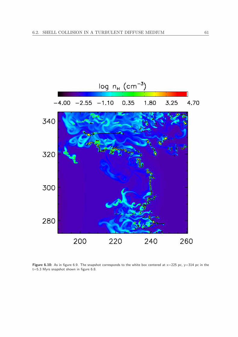
6.2. SHELL COLLISION IN A TURBULENT DIFFUSE MEDIUM 61
Figure 6.10: As in figure 6.9. The snapshot corresponds to the white box centered at x=225 pc, y=314 pc in thet=5.3 Myrs snapshot shown in figure 6.8.

62 CHAPTER 6. FORMATION OF COLD FILAMENTS FROM COLLIDING SHELLS
Figure 6.11: Time evolution of a single filament. The plots show logarithm of hydrogen number density. Theblack contour shows the level nH = 50 cm−3. From top left to bottom right: 4.3, 4.6, 5.3 and 7 Myrs after starformation. Note the change in scale between the snapshots.

6.2. SHELL COLLISION IN A TURBULENT DIFFUSE MEDIUM 63
Figure 6.12: Pressure versus hydrogen density of the fluid in the box for the turbulent medium run. The plot isfrom the last snapshot, 7 Myrs after star formation. The gas has been binned and color-coded according to themass fraction it represents. The solid line is the cooling-heating equilibrium curve for the warm and cold gas andthe dashed lines show the locations of three isotherms. Red crosses are average clump quantities.

64 CHAPTER 6. FORMATION OF COLD FILAMENTS FROM COLLIDING SHELLS
Figure 6.13: Gas fractions with time for the turbulent medium run. The dashed curve shows the mass fraction inthe warm gas phase, the solid curves shows the mass fraction in the hot gas phase and the dotted curve the massfraction in the cold phase. (Hot phase: gas with T ≥ 25000K, warm phase: gas with 100K < T < 25000K, coldphase: gas with T ≤ 100K)

6.2. SHELL COLLISION IN A TURBULENT DIFFUSE MEDIUM 65
they move towards pressure equilibrium with the surrounding medium in approximately asound crossing time, cs/L, where cs the sound speed and L the typical size of these clumps.For a typical density of 10−21 g/cm3 and a typical temperature of 50 K, the sound speed inthese clumps is about 0.8 km/sec. At this velocity sound waves will cross a 2 pc long clumpin about 0.6 Myrs. In the turbulent diffuse background run, clumps are formed later than inthe uniform background run, which means they are less evolved and farther from equilibrium.According to the above calculations, the time difference between clump formation betweenthe two simulations is about 3 sound crossing times, which is enough for many the clumps inthe uniform diffuse background simulation to have reached approximate pressure equilibriumwith the hot medium.
Figure 6.13 shows the evolution of the mass fractions of the gas in different temperatureregimes. Unlike the previous run, in this simulation there is a maximum in the hot gas massfraction at about 3.5 Myrs after star formation and a later minimum of the warm gas fractionat around 5 Myrs after star formation. This can be explained by the delayed formation ofcold gas in this simulation. Until the cold gas is formed, the hot gas just compresses the warmgas. Then the hot gas mass fraction increases, while the warm gas mass fraction decreases.When cold gas starts to form, it quickly dominates the mass, causing the warm and hot massfractions to drop.

66 CHAPTER 6. FORMATION OF COLD FILAMENTS FROM COLLIDING SHELLS

Chapter 7Morphological features of the cold clumps
7.1 General
Figure 6.5 shows that we form hundreds of clumps in each snapshot of the simulations. Thismakes it very difficult to study each of them in detail, especially since they are constantlymerging and splitting. However, we can make some general comments on the morphology ofthe identified clumps and look into some of their properties.
Clumps are generally at lower pressures with respect to their surrounding gas (– see Figures7.1, 7.2 7.3 and 7.4). This means that the Thermal Instability is still acting in these regions,causing them to condense further. Two examples of condensing clumps are shown in Figure7.1. Others (about 11% in the last snapshot of the uniform background run and 16% in theturbulent background run) are rotating. Two examples of rotating structures are shown inFigure 7.2. Rotation is either combined with compression or it introduces a centrifugal forcewhich makes the clump expand. Of the rotating cores in the last snapshots of the uniformand the turbulent background runs, about 25% and about 35% respectively are at the sametime condensing and the rest are expanding. In very few cases, less than 1%, the centrifugalforce exactly balances the force due to the pressure difference between the interior and theexterior of the clump.
A small fraction of the identified clumps are in pressure equilibrium with their surround-ings, at least at their most central parts. These clumps do not tend to host significant internalmotions (– Figure 7.4).
All clumps are surrounded by a warm corona which is more dilute than their cold centralregions and at an intermediate pressure between their pressure and the one of the surroundinggas. This corona usually surrounds more than one clump, indicating that they are parts oflarger structures, such as the ones illustrated in Figures 6.9, 6.10 and 6.11.
In the following we focus on the velocity dispersions, sizes and possible evolution of theclumps.

68 CHAPTER 7. MORPHOLOGICAL FEATURES OF THE COLD CLUMPS
Figure 7.1: Two examples of condensing clouds. Top panels show the logarithm of hydrogen number density inlog(cm−3) and bottom panels show the logarithm of thermal pressure in log(K cm−3). The black arrows show thevelocity field with the mean velocity of the central clump subtracted. Overplotted in black are the contour levelsfor nH equal to 50 cm−3, 100 cm−3 and 1000 cm−3.

7.1. GENERAL 69
Figure 7.2: Two examples of rotating clumps. Top panels show the logarithm of hydrogen number density inlog(cm−3) and bottom panels show the logarithm of thermal pressure in log(K cm−3). The black arrows show thevelocity field with the mean velocity of the central clump subtracted. Overplotted in black are the contour levelsfor nH equal to 50 cm−3, 100 cm−3 and 1000 cm−3.

70 CHAPTER 7. MORPHOLOGICAL FEATURES OF THE COLD CLUMPS
Figure 7.3: Two examples of clumps hosting random motions. Top panels show the logarithm of hydrogen numberdensity in log(cm−3) and bottom panels show the logarithm of thermal pressure in log(K cm−3). The black arrowsshow the velocity field with the mean velocity of the central clump subtracted. Overplotted in black are the contourlevels for nH equal to 50 cm−3, 100 cm−3 and 1000 cm−3.

7.1. GENERAL 71
Figure 7.4: Two examples of clumps with small internal velocities. Top panels show the logarithm of hydrogennumber density in log(cm−3) and bottom panels show the logarithm of thermal pressure in log(K cm−3). The blackarrows show the velocity field with the mean velocity of the central clump subtracted. Overplotted in black are thecontour levels for nH equal to 50 cm−3, 100 cm−3 and 1000 cm−3.

72 CHAPTER 7. MORPHOLOGICAL FEATURES OF THE COLD CLUMPS
Figure 7.5: Clump internal velocity dispersion versus their sound speed at different times. From top to bottom, 3,5 and 7 Myrs after star formation. The left panel corresponds to the uniform background medium run, the rightpanel to the turbulent background medium run.
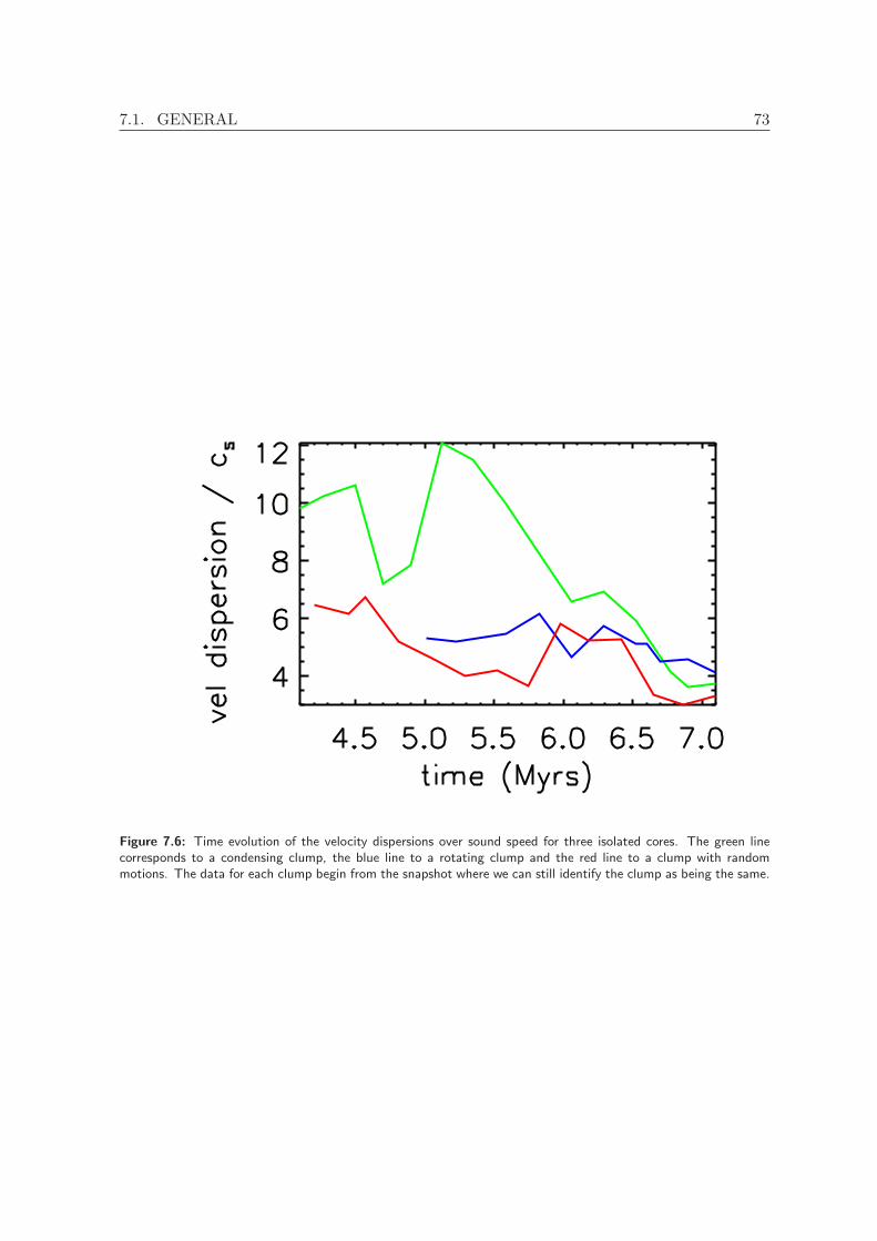
7.1. GENERAL 73
Figure 7.6: Time evolution of the velocity dispersions over sound speed for three isolated cores. The green linecorresponds to a condensing clump, the blue line to a rotating clump and the red line to a clump with randommotions. The data for each clump begin from the snapshot where we can still identify the clump as being the same.

74 CHAPTER 7. MORPHOLOGICAL FEATURES OF THE COLD CLUMPS
7.2 Velocity dispersions
Figure 7.5 shows the internal velocity dispersions of the clumps at different times for bothsimulations. The velocity dispersion in this context is defined as the square root of the varianceamong all locations which compose the clump. This means that for many clumps a velocitydispersion may indicate rotation, compression, expansion or random motions. As randommotions here we define any combination of rotation and compression or expansion. Since theclumps have no significant internal density fluctuations, mass-weighted velocity dispersionsare not very different from the ones presented here.
Although many of the formed clumps host supersonic motions in their interior at all times,there is an indication that these motions decrease at later times, as shown in the velocitydispersion plot of the last snapshots. This effect seems slightly more pronounced for theturbulent background run, where the largest internal velocity dispersions have disappearedin the last snapshot.
In the case of compression or expansion, this means that the clumps gradually move topressure equilibrium with their surrounding gas. In the case of random motions, it indicatesthat these motions were inherited by the turbulent environment that created the clumps but,in absence of any mechanism to sustain them, they die out. In the case of rotation, though,the situation is a bit more complicated. Rotation could be an effect of the large-scale Kelvin-Helmholtz shear, it can originate from Thermal Instability accretion or can be a result ofstructures splitting or merging. Angular momentum conservation sustains these motions forlonger, so we would only expect them to decrease on a viscous timescale.
In order to study if the decrease in internal velocity dispersion is observable for individualclumps, we tracked some of them back in time and plotted their velocity dispersion evolution.Since dense structures are created all the time and clumps merge or split at each snapshot, itis very difficult to construct an algorithm able to automatically identify a clump in differentsnapshots. Instead we identified the clumps by eye according to their positions and transla-tional velocities. We focus here on three examples: a rotating clump, a contracting clumpand a clump with random internal motions. Their velocity dispersions over their correspond-ing sound speed as a function of time are shown in Figure 7.6. Since clumps evolve almostisothermally, their sound speed does not vary significantly during the interval shown in theplot. The green line corresponds to a contracting clump, the blue line to a rotating clumpand the red line to a clump with random motions. All three clumps show some decrease invelocity dispersion with time. Although we are not able to make a complete study at thisstage, we observe that the rotating clump practically maintains the same velocity dispersionthroughout its existence, showing only a slight decrease, while the condensing clump and theclump with random motions show a decrease in velocity dispersion. For the condensing clumpthis decrease is especially pronounced.
7.3 Sizes
Figure 7.7 shows the size distribution of the clumps at different times for both simulations.The sizes are calculated as the square root of the area occupied by the clump. Although wedo not form clumps larger than approximately 3 pc, the maximum clump length can reachabout 10 pc. This means that structures may have one very large dimension, but they occupya very small area.

7.3. SIZES 75
Figure 7.7: Clump size distributions in parsecs at different times. The plot on the left-hand side corresponds tothe run in a uniform diffuse medium and the plot on the right to the run in a turbulent diffuse medium. The solidblack, dashed red and dash-dotted blue histograms correspond to the 3 Myrs, 5 Myrs and 7 Myrs, respectively.
Figure 7.8: Clump size over clump Jeans length distributions at different times. The plot on the left-hand sidecorresponds to the run in a uniform diffuse medium and the plot on the right to the run in a turbulent diffusemedium. The solid black, dashed red and dash-dotted blue histograms correspond to the 3 Myrs, 5 Myrs and 7Myrs, respectively.

76 CHAPTER 7. MORPHOLOGICAL FEATURES OF THE COLD CLUMPS
Figure 7.8 shows the distributions of the ratios of clump sizes over their correspondingJeans length, at different times. The size distributions of the clumps have a very similarshape and range between the two simulations. As clumps are fairly uniform in density andtemperature, their Jeans length does not vary significantly within a single clump. Clumps ingeneral seem to be smaller than their corresponding Jeans length but, as time advances, someof them become large enough to be potentially unstable to gravitational collapse. Of course,as we have not included gravity in these simulations we cannot know if this would actuallybe the case.
As mentioned earlier, since the formed structures are very filamentary, they are likely tocontain more Jeans lengths along a single dimension. Note also that the algorithm we use tofind clumps favors the identification of the smallest possible structures as separate entities.As mentioned above however, the clumps we identify are usually parts of larger structureswhich are dynamically interacting or surrounded by a common warm and more diffuse corona.
7.4 Clump evolution
Although most of the clumps are in low-pressure regions in the simulation, there are someclumps with approximately the same pressure as their surrounding gas. All of the clumps aresurrounded by an intermediate pressure corona, which is also thermally unstable.
This, in combination with the fact that clumps show a tendency of decreasing their internalmotions with time and that clouds in pressure equilibrium tend to host smaller internalmotions leads us to believe that there might be an evolution from clumps out of equilibrium,with strong internal motions to more quiescent clumps.
Figure 7.9 shows the tracks of the same three clumps we traced back in time, on thepressure-density diagram. The dotted line is the cooling-heating equilibrium curve. Thecold structures form in an area where cooling dominates, possibly from thermally unstablegas, at the left of the figure. As time goes by they move on the equilibrium curve andgradually increase their density and pressure, always staying on the curve. The timescaleof this evolution is about 2-3 Myrs, which corresponds to about 4 - 5 clump sound crossingtimes.

7.4. CLUMP EVOLUTION 77
Figure 7.9: Isolated core tracks on a pressure-density diagram. The green triangles correspond to a condensingclump, the blue crosses to a rotating clump and the red diamonds to a clump with random motions. The solid blackline is part the cooling-heating equilibrium curve which was shown in figures 6.3 and 6.12.

78 CHAPTER 7. MORPHOLOGICAL FEATURES OF THE COLD CLUMPS

Chapter 8Metal enrichment of the clouds
8.1 Setup of the simulation
A two-dimensional, high-resolution simulation very similar to those presented in the previousChapters, is performed using the same setup, namely two young OB associations placed at acertain distance from each other in a warm diffuse background. These cold and dense shellseventually collide in the middle of the computational domain. In this case though, each OBassociation comprises 20 ”average” stars, placed in a circular region of 5 pc radius and thephysical size of the domain is half that of the simulations in Chapters 6 and 7.
An important increase in efficiency in comparison to the previous simulations is achievedwith the use of Adaptive Mesh Refinement (AMR). Given the nature of the problem understudy, the most adequate refinement policy is to trigger the division of a oct when the dif-ference in the gradients of pressure and density exceeds a certain threshold. We have useda threshold equal to 1% in this work. Experimenting with the value of the threshold gaveno significant differences in the grid structure, although thresholds higher than 10% failed tocapture the shock structure properly.
The supershells in this setup are expanding in a uniform diffuse background, which meansthat any perturbations that are expected to seed the fluid instabilities we want to study mustarise at the grid level. In order then to make this simulation comparable to previous results,we should also seed the perturbations at the smallest grid level and the physical scale forseeding the perturbation should be the same between different runs. For this reason, weinitiate the simulation with a nested grid configuration, where the highest resolution regionis located at the center of the simulation box. Once the first seeds of the perturbation startto grow, we switch to the adaptive refinement policy described above.
Figure 8.1 shows the behavior of the three different grid configurations. The top row showsthe logarithm of hydrogen number density and the bottom row shows the corresponding gridstructure. The grid structure for the uniform grid run is, of course, trivial, but it is shown here
This chapter is an adaptation of the paper ”On the inefficiency of metal enrichment of cold gas in collidingflow simulations”, by E.Ntormousi and A. Burkert, to be submitted to the Astrophysical Journal.

80 CHAPTER 8. METAL ENRICHMENT OF THE CLOUDS
Figure 8.1: Snapshots of three runs using different refinement techniques, taken at the same timestep, about 3Myrs after star formation. From left to right, uniform grid, geometry-based refined and gradient-based refined grid.The plots on the top row show the logarithm of hydrogen number density and the plots on the bottom row showthe corresponding grid structure. The axes coordinates are in parsecs.

8.1. SETUP OF THE SIMULATION 81
Figure 8.2: Density (top) and pressure (bottom) histograms of the same snapshots shown in Figure 8.1, about 3Myrs after star formation. The solid black histograms correspond to the run with a uniform grid, the dashed redhistograms to the gradient-based AMR run and the dashed-dotted blue histograms to the geometry-based refinementrun.

82 CHAPTER 8. METAL ENRICHMENT OF THE CLOUDS
Figure 8.3: Gas mass fractions with time for three models. The black lines correspond to the run with a uniformgrid, the red lines to the gradient-based refinement run and the blue lines to the geometry-based refinement run.Dashed lines show the mass fraction of the gas in the warm phase, solid lines show the gas mass fraction in the hotphase and dashed-dotted lines show the gas mass fraction in the cold phase. (Hot phase: gas with T ≥ 25000 K,warm phase: gas with 100 K< T <25000 K, cold phase: gas with T < 100 K).

8.1. SETUP OF THE SIMULATION 83
anyway for completeness. The density and pressure gradient-based refinement works very wellin following the shocks and the locations where cold structure is formed (rightmost panel ofFigure 8.1). However, the small-scale noise introduced by the interpolation, in combinationwith the nonlinear nature of the gas dynamics in this environment leads to slight differencesin the morphology of the gas between the uniform and the adaptively refined grid at the sametimestep.
There is a minimum resolution below which cold gas does not form at the edges of theshells at all, evident in the run with a nested grid configuration (middle panel of Figure 8.1).In the regions where the grid size is too large the shocks are smoothed out, suppressing theVishniac Instability and preventing the gas at the edges of the shells from becoming thermallyunstable.
The volume fractions of the gas in each phase are practically identical between the uniformgrid and the gradient-refined grid simulations (Figure 8.2), however the gas in the uniformgrid run is allowed to condense to slightly higher densities, as shown by the density histogramon the top panel of Figure 8.2. The nested grid simulation has significantly less gas in thehigh-density regime in comparison, due to the lower resolution in the top and bottom partsof the grid.
The corresponding pressure histograms for the three runs are shown on the bottom panelof Figure 8.2. Again, the uniform grid run and the gradient-defined AMR runs seem to agreealmost completely, but the geometry-based refinement run has a slightly different configura-tion, with a lot of gas in the thermally unstable regime, unable to condense and cool further.This is indicative of the result one might get from cooling shock simulations if the resolutionis insufficient to capture the initial density enhancements.
The mass fractions of the gas in different temperature regimes are plotted in Figure 8.3.The dotted-dashed lines in this Figure correspond to the cold gas (T < 100 K), which formssmall dense clumps, the dashed lines correspond to the warm gas (100 K< T <25000 K),mainly consisting of the background gas and the coronas around the cold clumps, and thesolid lines correspond to the hot gas (T ≥ 25000 K), mainly located in the wind and theshocked areas. Black color denotes the uniform grid run, blue the geometry-based refinementrun and red the gradient-based refinement run. The mass fractions in different phases seem toagree between the uniform grid and the gradient-based grid runs during the whole simulationtime, with the cold gas dominating the mass towards the end of the simulation (about 80%of the total mass). However, the nested grid run fails to reach these high mass fractions dueto the very low resolution in part of the domain.
In conclusion, the comparison between simulations of this setup with AMR and withuniform grid simulations have shown no difference in the amount of cold gas, the position ofthe shocks and the sizes or velocity dispersions of the formed clumps. Small differences in theshock morphology are, of course, always present, due to the very nonlinear nature of thesephenomena.
For this particular simulation we use a box of 250 pc physical size, at an effective resolutionof 20482. The choice of a smaller box with respect to Paper I is not only more physical, interms of the average distance between OB associations in the Galaxy but it also yields asmaller computational volume for the same physical resolution, significantly reducing thecomputational cost of the simulation.
We stop the calculation when the turbulence in the collision area starts to expand towardsthe inflow boundaries. In this particular case this happens 4.36 Mys since star formation inthe OB associations.

84 CHAPTER 8. METAL ENRICHMENT OF THE CLOUDS
As mentioned before, the aim of this work is to study the advection of metals from theOB associations to the cold gas formed at the shock wake. This is done by means of a passiveadvected quantity, representing the metal injection from the stars. A constant amount ofmetals, equal to 10−3 metal particles/cm3 is added at the wind region at each coarse timestep.As this value is totally arbitrary, it can be weighted to simulate different environments.
The amount of metals introduced by the OB associations is assumed here to have anegligible effect on the amount of cold gas formed. In principle, though, extra metals couldaffect our results due to their contribution to the cooling, which would also change the regimewhere the gas becomes thermally unstable. In our calculations the most important coolant ofthe gas is line emission from carbon and oxygen. A decrease in the abundance of these elementswould cause the area where we can have phase formation due to the Thermal Instability toshrink, and an enrichment would enlarge the Thermal Instability regime (Wolfire et al., 1995).
Support for the approximation we are making comes from Walch et al. (2011b), whostudied the effect of metallicity on the formation of cold gas from Thermal Instability insimulations of turbulence. They found that, for driven turbulence (which is the case in ourmodels), the total amount of cold gas in the simulation is not significantly affected by changesin the metallicity. This means that, as long as the metallicity of the gas we are simulatingis high enough to capture the Thermal Instability regime of the ISM, we are not makingsignificant errors in the total amount of cold gas in the domain by ignoring the enrichmentfrom the OB stars in the cooling function.
8.2 Metal enrichment of the gas from the OB associations
Figure 8.4 shows snapshots of the simulation before and after the shell collision. The toppanels of this Figure are contours of the logarithm of the gas temperature and the bottompanels show the logarithm of the ratio of metal to hydrogen atoms in the cell.
The general picture of the simulation is the same as in Paper I. The spherical shocks cre-ated by the stellar feedback are unstable to the Vishniac instability (Vishniac, 1983, 1994) assmall-scale wind imperfections create ripples on their surface. The result of the gas condensa-tion at the peaks of these ripples is to trigger the Thermal Instability (Field, 1965), creatingcold and dense clumps at the shock wake. The shear on the shell surface, also caused by theVishniac Instability, gives rise to characteristic Kelvin-Helmholtz eddies, thus contributing tothe dynamics of the newly-formed cold clumps (left panel of Figure 8.4).
When the shells collide, the combination of the large-scale shear by the collision andthe small-scale structure already present in the shells gives rise to a turbulent region atthe collision interface which contains both warm and cold gas (right panel of Figure 8.4).Turbulence is a very efficient mixing mechanism, so we naturally expect an enhancement inmetallicity of the warm gas after the shell collision.
In Figure 8.4, we can indeed see that the warm gas has enhanced metal content. Thesame can be shown more clearly by plotting the mass fraction of the gas in the computationaldomain in density-metallicity bins. In Figure 8.5, showing such plots for two snapshots of thesimulation, we can see that the dense gas dominates the mass of the gas in the computationaldomain. At the same time we see that it never reaches relative enrichment of more than 10−4.For comparison, we note that, were the metals ejected by the stars to be instantaneously andhomogeneously mixed in the diffuse gas phase, the relative enrichment would be 10−2 andif all the metals from the stars ended up in the cold phase, the relative enrichment of that

8.2. METAL ENRICHMENT OF THE GAS FROM THE OB ASSOCIATIONS 85
Figure 8.4: Logarithm of temperature (top) and logarithm of relative metal content (bottom) for two snapshots.On the left, 1.22 Myrs and on the right, 4.46 Myrs after star formation took place in the OB associations.

86 CHAPTER 8. METAL ENRICHMENT OF THE CLOUDS
phase would be of about 5 · 10−2.Throughout the simulation practically all the metals injected by the OB associations stay
in the hot wind, despite the fact that most of the mass is in the cold gas component. Atlate times a small fraction of the metals (1-5%) mixes into the slightly denser, warm gas(nH ≃ 10−1, T ≃ 105) due to the shell collision that causes turbulent mixing.
8.3 Metal enrichment of the clumps
A clump is identified as a collection of adjacent cells with densities above 50 cm−3 andtemperatures lower than 100 K. By this definition alone, Figure 8.5 already indicates thatthe clumps do not contain significant amounts of material from the OB associations.
To look at the clump metallicities in more detail, we plot their metallicity distributions,shown in Figure 8.6. The top panels in this Figure show the distributions of the meanabsolute metal content of the clumps, in the arbitrary units chosen in this simulation for themetallicity (10−3/cm3 injected in the wind domain at each timestep) and the bottom panelsshow distributions of the mean metallicity over the mean hydrogen number density of theclumps. The plots on the left-hand side correspond to the snapshot at 1.22 Myrs and theplots on the right-hand side to the final snapshot, at 4.36 Myrs.
Even though the numbers can be rescaled to mean different absolute metal content in theclumps, the important fact here is that the cold phase will always receive at least two ordersof magnitude less metals than the diffuse warm phase.
Even though the metal injection from the OB associations does not stop during the sim-ulation time, the metal content of the clumps does not seem to increase significantly. Thespread of the distribution of the relative metal content of the clumps seems to increase withtime. As the system evolves, new clumps are formed at relatively lower metallicities. Thelittle metals they accumulate over time leads to the formation of a peak in the distribu-tion. However, the maximum value of the distribution does not increase, meaning there is nosignificant enrichment.
Figures 8.7 and 8.8 show the mean number density of metals in a clump as a functionof distance from its closest OB association and as a function of the polar angle with respectto the horizontal line in the middle of the domain, respectively. The amount of metals in aclump does not seem to depend on its position with respect to the OB associations, pointingto a very uniform distribution of metallicities around the young associations.

8.3. METAL ENRICHMENT OF THE CLUMPS 87
Figure 8.5: Mass fractions in density-metallicity bins at two snapshots, 1.22 Myrs (top) and 4.36 Myrs (bottom)after star formation.

88 CHAPTER 8. METAL ENRICHMENT OF THE CLOUDS
Figure 8.6: Top: Distributions of the absolute metal content of the clumps. Bottom: Distributions of the metalcontent of the clumps over their hydrogen number density. The data are from snapshots 1.22 Myrs (left) and 4.36Myrs (right) after star formation.
Figure 8.7: Dependence of the clump metal content on their distance from the closest association. The plots areshown at 1.22 Myrs (left) and 4.36 Myrs (right) since the beginning of the simulation.

8.3. METAL ENRICHMENT OF THE CLUMPS 89
Figure 8.8: Dependence of the clump metal content on their polar angle calculated with respect to the horizontalline at the center of the computational domain. The plots are shown at 1.22 Myrs (left) and 4.36 Myrs (right) sincethe beginning of the simulation.

90 CHAPTER 8. METAL ENRICHMENT OF THE CLOUDS

Chapter 9Summary and Conclusions
In this text we have presented our work on the formation of cold structure from large-scalecolliding flows. In particular, we have shown the results of detailed numerical simulations ofcolliding superbubbles. These large cavities of hot gas are created by the violent feedbackfrom young massive stars, implemented as a time-dependent energy and mass source in apublic hydrodynamics code. The extremely dynamical evolution of the gas was followed tothe point of the fragmentation and collision of the dense shells.
Our results provide a picture of the ISM similar to that in Audit & Hennebelle (2005)and Hennebelle & Audit (2007b), where the ISM phases are tightly interwoven, with sharpthermal interfaces between them. Of course, a more detailed comparison is not possible, sincethat work was done with a much higher resolution, representing a smaller region of the ISMand not including the hot phase. In our simulations, elongated cold structures sit in warm,thermally unstable coronas, submerged in a hot dilute medium that the stellar winds andsupernovae from young OB stars create. Clumps are dynamical entities, constantly mergingand splitting and in general not in pressure equilibrium with their surrounding gas. In thatsense, the picture we see in our simulations is very different from the classical ISM modelproposed by McKee & Ostriker (1977), where the clouds are treated as quasi-static spheres.The structures we find are rather long thin filaments, very similar to the large ”blobby sheets”proposed by Heiles & Troland (2003).
We identify individual clumps in the simulations by setting density and temperaturethresholds and connecting adjacent locations in the simulation domain which exceed thesethresholds. This method favors the identification of the smallest cold and dense structures.The clumps tend to be connected in groups within a common warm corona, forming longfilaments and are mostly located in areas of lower pressure with respect to their surroundings.The latter causes many of them to condense to higher densities and smaller volumes, almostisothermally. Apart from condensing clumps we find rotating clumps, as well as clumpshosting irregular motions. All these internal motions are reflected in the velocity dispersion assupersonic internal motions. Approximately 11 to 16% of the identified clumps are rotatingand are interesting candidates for forming protostellar disks. However, rotation should bestudied in three dimensions for more reliable results.
Internal clump motions tend to decrease with time, as the clumps come closer to thermalpressure equilibrium with their warm surroundings. However, if gravity and star formation

92 CHAPTER 9. SUMMARY AND CONCLUSIONS
was included in our simulations, we would expect these motions to be sustained for longertimes due to gravitational collapse and feedback from the newly formed stars in their interior.
Cold clumps in our simulations form by Thermal Instability condensation of the ambientdiffuse medium when it is perturbed by the expanding shells. This, in combination with thefact that the mass injected by the OB associations is a very small fraction of the total massin our domain throughout the simulation, shows that the material forming the new clumpscould not have been enriched directly by the supernova explosions. The material ejected fromthe OB associations will probably enrich the interstellar matter on much larger timescales,after the hot bubbles have mixed with the diffuse medium.
In order to study of metal advection from the hot to the cold ISM, we have presenteda simulation of the same setup, using an advected quantity. This quantity was inserted inthe region of the domain representing the wind, to represent the metals ejected by the windsand supernova explosions in these OB associations. In this way, we were able to distinguishbetween material originating from the stars and material originating from the diffuse ISM inthe composition of the cold clumps.
We have found that the metal content of the clumps is very low throughout the simulation.The maximum metal to hydrogen number ratio reached in the simulation is about 10−4, twoorders of magnitude lower than the value of the same ratio for the warm diffuse medium. Thefact that the diffuse gas receives a significant fraction of the injected metals implies that, ifmolecular clouds were to form in this environment, significant enrichment would be delayedby at least one stellar generation. This effect is even more relevant if we consider that thefree-fall time for each of these dense clumps is about 1 Myr, which means that many of themwould be collapsing before the end of this simulation, had gravity been considered, leavingeven less time for enrichment.
The metal content of the clumps seems to be independent of their position with respect tothe OB association. This, in combination with the small spread in cloud metallicities, meansthat the next stellar generation, formed by the clumps created in such an environment, wouldbe very uniform in its metal content, provided the diffuse component is also well mixed.
Of course, there are many effects that have not been included in this work. For instance,we have assumed that the metal injection from the OB associations is roughly constant withtime and that it is uniformly distributed in the wind region. Both these assumptions arequestionable. We would, in principle, expect the metals to be contained in small clumps,as part of clumpy winds or fast supernova ejecta, possibly making mixing more efficient. Inaddition, the wind material should of course differ in quantities and composition from thesupernova material, although this would still mostly end up in the diffuse rather than thedense cold phase. These are all complications that should be taken into account in futurework.
Thermally unstable gas amounts to about 8 to 10% of the total gas mass in the lastsnapshots of our simulations, far from the almost 50% that is commonly detected in observa-tions (Heiles & Troland, 2003) or found in simulations of turbulent, thermally bistable flows(Gazol et al., 2001, 2005). This is because our simulations are dominated by what we identifyas CNM, that is, gas with temperatures lower than 100K. Due to our very high resolution,this gas is also very dense, reaching hydrogen number densities of the order of 105 cm−3.This gas would be mostly molecular, so it would not be identified as cold HI in observations.In simulations with gravity we would not expect to encounter this issue, since gravity wouldeventually dominate the dynamics of the formed clumps and turn them into stars once theybecame dense enough, so thermal instability would no longer be responsible for their evolution

93
at these densities.The simulations presented here are only a first step to modeling triggered molecular cloud
formation using physically motivated colliding flow parameters. We have not attempted aparameter study in this paper, but it will be the object of future work to study the effect ofvarying the distance between the superbubbles, the number of OB stars creating the super-bubbles and the metallicity of the gas.
In this work we have also not taken into account galactic shear or density stratification.Assuming a galactic rotation rate of 26 km sec −1 kpc −1, the relative shear in our computa-tional box would be 13 km sec−1. This velocity would have a crossing time of approximately37 Myrs, which is much longer than what our simulations last. Density stratification witha scale height of H=150pc would cause the superbubbles to expand faster along the verticaldirection, but since we are interested mostly in what happens at the superbubble collisioninterface, we can neglect this effect as a first approximation.
Our calculations also ignore magnetic fields and gravity. s We would expect magneticfields to play a significant role in the dynamics of the problem, both during the expansion ofthe superbubbles and also during the more complex collision phase, if they had a preferredorientation, but in two dimensions we would not be able to model all relevant phenomenaproperly anyway. Gravity is essential for studying the evolution of the clumps and for esti-mating their star forming efficiency. Combining with the modeling of a third dimension, itwould give us useful mass estimates of the formed structures. Moving to three dimensionsand including gravity is work in process and will be presented in a future paper.
We find the main limitations of our work to be the lack of resolution and bidimensionality.As we have pointed out, our simulations do not reach the resolution required to capture allthe relevant physical processes on the smallest scales. We have accounted for small-scaleeffects by only studying clumps which contain more than 16 grid cells. Higher numericalresolution will certainly provide more insight on the number of formed clumps and theirinternal structure. Although numerical effects do introduce a thermal conduction effect,explicitly modeling thermal conduction would help set the minimum scale for formed clumpsand achieve convergence with increasing resolution. On the other hand, if gravity is simulatedit will probably already become important at length scales larger than the Field length.
The restriction of the presented models to two dimensions is emphasizing the formation offilaments. In three dimensions, these structures could have a sheet-like morphology. Gravitycould then be responsible for turning these sheets into filaments (Burkert & Hartmann, 2004;Hartmann & Burkert, 2007; Heitsch et al., 2008b).

94 CHAPTER 9. SUMMARY AND CONCLUSIONS
Bibliography
Alves, J., Lombardi, M., & Lada, C. J. 2007: The mass function of dense molecular coresand the origin of the IMF, A&A, 462, L17
Audit, E. & Hennebelle, P. 2005: Thermal condensation in a turbulent atomic hydrogen flow,A&A, 433, 1
Ballesteros-Paredes, J., Hartmann, L., & Vazquez-Semadeni, E. 1999: Turbulent Flow-drivenMolecular Cloud Formation: A Solution to the Post-T Tauri Problem?, ApJ, 527, 285
Burkert, A. 2006: The turbulent interstellar medium, Comptes Rendus Physique, 7, 433
Burkert, A. & Hartmann, L. 2004: Collapse and Fragmentation in Finite Sheets, ApJ, 616,288
Burkert, A. & Lin, D. N. C. 2000: Thermal Instability and the Formation of Clumpy GasClouds, ApJ, 537, 270
Chandrasekhar, S. 1961, Hydrodynamic and hydromagnetic stability, ed. Chandrasekhar, S.
Churchwell, E., Babler, B. L., Meade, M. R., Whitney, B. A., Benjamin, R., Indebetouw,R., Cyganowski, C., Robitaille, T. P., Povich, M., Watson, C., & Bracker, S. 2009: TheSpitzer/GLIMPSE Surveys: A New View of the Milky Way, PASP, 121, 213
Churchwell, E., Povich, M. S., Allen, D., Taylor, M. G., Meade, M. R., Babler, B. L., Inde-betouw, R., Watson, C., Whitney, B. A., Wolfire, M. G., Bania, T. M., et al. 2006: TheBubbling Galactic Disk, ApJ, 649, 759
Dale, J. E., Wunsch, R., Smith, R. J., Whitworth, A., & Palous, J. 2011: The fragmentationof expanding shells - III. Oligarchic accretion and the mass spectrum of fragments, MNRAS,411, 2230
Dale, J. E., Wunsch, R., Whitworth, A., & Palous, J. 2009: The fragmentation of expandingshells - I. Limitations of the thin-shell approximation, MNRAS, 398, 1537
Dalgarno, A. & McCray, R. A. 1972: Heating and Ionization of HI Regions, ARA&A, 10, 375
de Avillez, M. A. & Breitschwerdt, D. 2004: 3D HD and MHD Adaptive Mesh RefinementSimulations of the Global and Local ISM, in Astrophysics and Space Science Library, Vol.315, How Does the Galaxy Work?, ed. E. J. Alfaro, E. Perez, & J. Franco, 331–+

96 BIBLIOGRAPHY
Dobbs, C. L., Burkert, A., & Pringle, J. E. 2011: Why are most molecular clouds not gravi-tationally bound?, MNRAS, 413, 2935
Draine, B. T. 2011: Astronomical Models of PAHs and Dust, in EAS Publications Series,Vol. 46, EAS Publications Series, ed. C. Joblin & A. G. G. M. Tielens, 29–42
Ehlerova, S. & Palous, J. 2005: H I shells in the outer Milky Way, A&A, 437, 101
Elmegreen, B. G. 1994: A Q condition for long-range propagating star formation, ApJ, 427,384
Elmegreen, B. G. & Lada, C. J. 1977a: Sequential formation of subgroups in OB associations,ApJ, 214, 725
Elmegreen, B. G. & Lada, C. J. 1977b: Sequential formation of subgroups in OB associations,ApJ, 214, 725
Falgarone, E. & Phillips, T. G. 1990: A signature of the intermittency of interstellar turbulence- The wings of molecular line profiles, ApJ, 359, 344
Ferriere, K. M. 2001: The interstellar environment of our galaxy, Reviews of Modern Physics,73, 1031
Field, G. B. 1965: Thermal Instability., ApJ, 142, 531
Frisch, U. 1996, Turbulence, ed. Frisch, U.
Gazol, A., Vazquez-Semadeni, E., & Kim, J. 2005: The Pressure Distribution in ThermallyBistable Turbulent Flows, ApJ, 630, 911
Gazol, A., Vazquez-Semadeni, E., Sanchez-Salcedo, F. J., & Scalo, J. 2001: The TemperatureDistribution in Turbulent Interstellar Gas, ApJ, 557, L121
Hartmann, L. 2002: Flows, Fragmentation, and Star Formation. I. Low-Mass Stars in Taurus,ApJ, 578, 914
Hartmann, L., Ballesteros-Paredes, J., & Bergin, E. A. 2001: Rapid Formation of MolecularClouds and Stars in the Solar Neighborhood, ApJ, 562, 852
Hartmann, L. & Burkert, A. 2007: On the Structure of the Orion A Cloud and the Formationof the Orion Nebula Cluster, ApJ, 654, 988
Haud, U. & Kalberla, P. M. W. 2007: Gaussian decomposition of H I surveys. III. Local H I,A&A, 466, 555
Heiles, C. 1979: H I shells and supershells, ApJ, 229, 533
Heiles, C. 1984: H I shells, supershells, shell-like objects, and ’worms’, ApJS, 55, 585
Heiles, C. & Troland, T. H. 2003: The Millennium Arecibo 21 Centimeter Absorption-LineSurvey. II. Properties of the Warm and Cold Neutral Media, ApJ, 586, 1067
Heitsch, F., Hartmann, L. W., & Burkert, A. 2008a: Fragmentation of Shocked Flows: Grav-ity, Turbulence, and Cooling, ApJ, 683, 786

BIBLIOGRAPHY 97
Heitsch, F., Hartmann, L. W., Slyz, A. D., Devriendt, J. E. G., & Burkert, A. 2008b: Cooling,Gravity, and Geometry: Flow-driven Massive Core Formation, ApJ, 674, 316
Heitsch, F., Slyz, A. D., Devriendt, J. E. G., Hartmann, L. W., & Burkert, A. 2006: TheBirth of Molecular Clouds: Formation of Atomic Precursors in Colliding Flows, ApJ, 648,1052
Hennebelle, P. & Audit, E. 2007a: On the Structure of the Interstellar Atomic Gas, in As-tronomical Society of the Pacific Conference Series, Vol. 365, SINS - Small Ionized andNeutral Structures in the Diffuse Interstellar Medium, ed. M. Haverkorn & W. M. Goss,133–+
Hennebelle, P. & Audit, E. 2007b: On the structure of the turbulent interstellar atomichydrogen. I. Physical characteristics. Influence and nature of turbulence in a thermallybistable flow, A&A, 465, 431
Hollenbach, D. J. & Thronson, Jr., H. A., eds. 1987, Astrophysics and Space Science Library,Vol. 134, Interstellar processes; Proceedings of the Symposium, Grand Teton National Park,WY, July 1-7, 1986
Kennicutt, Jr., R. C., Calzetti, D., Walter, F., Helou, G., Hollenbach, D. J., Armus, L.,Bendo, G., Dale, D. A., Draine, B. T., Engelbracht, C. W., Gordon, K. D., et al. 2007:Star Formation in NGC 5194 (M51a). II. The Spatially Resolved Star Formation Law, ApJ,671, 333
Kim, W. & Ostriker, E. C. 2002: Formation and Fragmentation of Gaseous Spurs in SpiralGalaxies, ApJ, 570, 132
Kim, W. & Ostriker, E. C. 2006: Formation of Spiral-Arm Spurs and Bound Clouds inVertically Stratified Galactic Gas Disks, ApJ, 646, 213
Klessen, R. S. 2001: The Formation of Stellar Clusters: Mass Spectra from Turbulent Molec-ular Cloud Fragmentation, ApJ, 556, 837
Kochanek, C. S. 2011: The Astrophysical Implications of Dust Formation during the Eruptionsof Hot, Massive Stars, ApJ, 743, 73
Kolmogorov, A. 1941: The Local Structure of Turbulence in Incompressible Viscous Fluid forVery Large Reynolds’ Numbers, Akademiia Nauk SSSR Doklady, 30, 301
Koyama, H. & Inutsuka, S. 2004: The Field Condition: A New Constraint on Spatial Reso-lution in Simulations of the Nonlinear Development of Thermal Instability, ApJ, 602, L25
Lada, C. J., Alves, J., & Lada, E. A. 1999: Infrared Extinction and the Structure of the IC5146 Dark Cloud, ApJ, 512, 250
Lada, C. J., Alves, J. F., & Lombardi, M. 2007: Near-Infrared Extinction and MolecularCloud Structure, Protostars and Planets V, 3
Landau, L. D. & Lifshitz, E. M. 1959, Fluid mechanics, ed. Landau, L. D. & Lifshitz, E. M.
Larson, R. B. 1981: Turbulence and star formation in molecular clouds, MNRAS, 194, 809

98 BIBLIOGRAPHY
Lequeux, J. 2005, The interstellar medium, ed. Lequeux, J.
Mac Low, M., Klessen, R. S., Burkert, A., & Smith, M. D. 1998: Kinetic Energy Decay Ratesof Supersonic and Super-Alfvenic Turbulence in Star-Forming Clouds, Physical ReviewLetters, 80, 2754
McCray, R. & Kafatos, M. 1987a: Supershells and propagating star formation, ApJ, 317, 190
McCray, R. & Kafatos, M. 1987b: Supershells and propagating star formation, ApJ, 317, 190
McKee, C. F. & Ostriker, J. P. 1977: A theory of the interstellar medium - Three componentsregulated by supernova explosions in an inhomogeneous substrate, ApJ, 218, 148
Molinari, S., Swinyard, B., Bally, J., Barlow, M., Bernard, J., Martin, P., Moore, T., Noriega-Crespo, A., Plume, R., Testi, L., Zavagno, A., et al. 2010: Hi-GAL: The Herschel InfraredGalactic Plane Survey, PASP, 122, 314
Nigra, L., Gallagher, III, J. S., Smith, L. J., Stanimirovic, S., Nota, A., & Sabbi, E. 2008:NGC 602 Environment, Kinematics and Origins, PASP, 120, 972
Ntormousi, E., Burkert, A., Fierlinger, K., & Heitsch, F. 2011: Formation of Cold FilamentaryStructure from Wind-blown Superbubbles, ApJ, 731, 13
Ntormousi, E. & Sommer-Larsen, J. 2010: Hot gas haloes around disc galaxies: O VII columndensities from galaxy formation simulations, MNRAS, 409, 1049
Padoan, P. 1995: Supersonic turbulent flows and the fragmentation of a cold medium, MN-RAS, 277, 377
Parmentier, G. 2011: From the molecular-cloud- to the embedded-cluster-mass function witha density threshold for star formation, MNRAS, 413, 1899
Pringle, J. E., Allen, R. J., & Lubow, S. H. 2001: The formation of molecular clouds, MNRAS,327, 663
Salpeter, E. E. 1977: Formation and destruction of dust grains, ARA&A, 15, 267
Schneider, S. & Elmegreen, B. G. 1979: A catalog of dark globular filaments, ApJS, 41, 87
Sutherland, R. S. & Dopita, M. A. 1993: Cooling functions for low-density astrophysicalplasmas, ApJS, 88, 253
Teyssier, R. 2002: Cosmological hydrodynamics with adaptive mesh refinement. A new highresolution code called RAMSES, A&A, 385, 337
Tielens, A. G. G. M. 2005, The Physics and Chemistry of the Interstellar Medium, ed. Tielens,A. G. G. M.
Vazquez-Semadeni, E., Gomez, G. C., Jappsen, A. K., Ballesteros-Paredes, J., Gonzalez,R. F., & Klessen, R. S. 2007: Molecular Cloud Evolution. II. From Cloud Formation to theEarly Stages of Star Formation in Decaying Conditions, ApJ, 657, 870

BIBLIOGRAPHY 99
Vazquez-Semadeni, E., Ryu, D., Passot, T., Gonzalez, R. F., & Gazol, A. 2006: MolecularCloud Evolution. I. Molecular Cloud and Thin Cold Neutral Medium Sheet Formation, ApJ,643, 245
Verschuur, G. L. 2004: Interstellar Neutral Hydrogen Emission Profile Structure, AJ, 127,394
Vishniac, E. T. 1983: The dynamic and gravitational instabilities of spherical shocks, ApJ,274, 152
Vishniac, E. T. 1994: Nonlinear instabilities in shock-bounded slabs, ApJ, 428, 186
Vishniac, E. T. & Ryu, D. 1989: On the stability of decelerating shocks, ApJ, 337, 917
Voss, R., Diehl, R., Hartmann, D. H., Cervino, M., Vink, J. S., Meynet, G., Limongi, M.,& Chieffi, A. 2009: Using population synthesis of massive stars to study the interstellarmedium near OB associations, A&A, 504, 531
Walch, S., Whitworth, A. P., & Girichidis, P. 2011a: The influence of the turbulent perturba-tion scale on pre-stellar core fragmentation and disc formation, MNRAS, 1725
Walch, S., Wunsch, R., Burkert, A., Glover, S., & Whitworth, A. 2011b: The Turbulent Frag-mentation of the Interstellar Medium: The Impact of Metallicity on Global Star Formation,ApJ, 733, 47
Whitworth, A. P., Bhattal, A. S., Chapman, S. J., Disney, M. J., & Turner, J. A. 1994:Fragmentation of shocked interstellar gas layers., A&A, 290, 421
Williams, J. P., Blitz, L., & McKee, C. F. 2000: The Structure and Evolution of MolecularClouds: from Clumps to Cores to the IMF, Protostars and Planets IV, 97
Wolfire, M. G., Hollenbach, D., McKee, C. F., Tielens, A. G. G. M., & Bakes, E. L. O. 1995:The neutral atomic phases of the interstellar medium, ApJ, 443, 152
Wong, T. & Blitz, L. 2002: The Relationship between Gas Content and Star Formation inMolecule-rich Spiral Galaxies, ApJ, 569, 157
Wunsch, R., Dale, J. E., Palous, J., & Whitworth, A. P. 2010: The fragmentation of expandingshells - II. Thickness matters, MNRAS, 407, 1963
Yang, C., Gruendl, R. A., Chu, Y., Mac Low, M., & Fukui, Y. 2007: Large-Scale GravitationalInstability and Star Formation in the Large Magellanic Cloud, ApJ, 671, 374
Zuckerman, B. & Evans, II, N. J. 1974: Models of massive molecular clouds, ApJ, 192, L149


Acknowledgments
This thesis represents the efforts of the last four years and signifies the beginning of myresearch career. It would have been impossible for me though to reach this point without thesupport of several people in my environment. I take this opportunity to thank them.
I am grateful to my PhD advisor, Andreas Burkert, for all our interesting discussions,for sharing his excitement for science with me and for helping my growth as an independentresearcher with his sincere support.
I received a lot of practical help for my thesis work from Fabian Heitsch. Not only didhe help me gain insight into the physics of the ISM by sharing his experience with me, buthe also trusted me with some of his codes. In particular, the calculations of the cooling andheating rates, as explained in Chapter 2 have been calculated with his code.
Katharina Fierlinger shared her PhD work on implementing stellar feedback in RAMSESwith me. Without her contribution a lot of this work would not have been possible. Inaddition, her careful observations significantly improved this work. Of course, I am alsograteful to Rasmus Voss for providing the stellar feedback data for this work and for beingalways available for questions regarding his calculations.
I also thank all my friends and colleagues here at the LMU Observatory, Thorsten Naab,Peter Johansson and Roland Jesseit, not only for techical advice, but also for all the fun wehave had these years and for their kind words of advice at hard times.
To my Physics Diploma supervisor at the Aristotle University of Thessaloniki, LoukasVlahos, an eternal ”thank you” for believing in me from the start and for encouraging me topursue a career as a scientist.
To my family, all my love and gratitude for always being there for me and for all thesacrifices they’ve made so that I can fulifill my dreams.
Finally, to my partner, Jose Luis Pinar, a big thank you from my heart for your faith inme, for your support and understanding. I would never have reached this far without you.

Curriculum Vitae
Personal
Name: Evangelia Ntormousi
Born: 31st of March, 1984
Citizenship: Greek
Address: Scheinerstr. 1, Munich, Germany D-81679
Education
2007–date Ph.D in Astrophysics International Max Planck Research School(IMPRS), USM-LMU
2001–2007 Bachelor and Masters in Physics Aristotle University Thessaloniki, Greece
Publications
• E. Ntormousi, A. Burkert, On the inefficiency of metal enrichment in colliding flowsimulations, in prep.
• E. Ntormousi, A. Burkert, K. Fierlinger and F. Heitsch, Formation of cold filamentarystructure from wind-blown superbubbles, ApJ, 731, 13
• E. Ntormousi, J. Sommer-Larsen, Hot gas haloes around disc galaxies, 2010, MNRAS,409, 1049