formally assessing cryptographic entropy · 2013-01-02 · formally assessing cryptographic entropy...
TRANSCRIPT

Formally Assessing Cryptographic Entropy
Daniel R. L. Brown∗
January 2, 2013
Abstract
Cryptography relies on the secrecy of keys. Measures of information, and thus secrecy, are called entropy.Previous work does not formally assess the cryptographically appropriate entropy of secret keys.
This report defines several new forms of entropy appropriate for cryptographic situations. This report definesstatistical inference methods appropriate for assessing cryptographic entropy.
Contents
1 Introduction 51.1 Further Motivation . . . . . . . . . . . . . . . . . . . . . . . . . . . . . . . . . . . . . . . . . . . . . . . 5
1.1.1 Roles of Entropy in Cryptography . . . . . . . . . . . . . . . . . . . . . . . . . . . . . . . . . . 51.1.2 Entropy Source Examples . . . . . . . . . . . . . . . . . . . . . . . . . . . . . . . . . . . . . . . 8
1.2 Previous Work . . . . . . . . . . . . . . . . . . . . . . . . . . . . . . . . . . . . . . . . . . . . . . . . . 111.2.1 Hypothesis Testing . . . . . . . . . . . . . . . . . . . . . . . . . . . . . . . . . . . . . . . . . . . 111.2.2 Randomness Extraction . . . . . . . . . . . . . . . . . . . . . . . . . . . . . . . . . . . . . . . . 121.2.3 Entropy Assessment . . . . . . . . . . . . . . . . . . . . . . . . . . . . . . . . . . . . . . . . . . 12
1.3 Overview of this Report . . . . . . . . . . . . . . . . . . . . . . . . . . . . . . . . . . . . . . . . . . . . 131.3.1 Contributions . . . . . . . . . . . . . . . . . . . . . . . . . . . . . . . . . . . . . . . . . . . . . . 131.3.2 Organization . . . . . . . . . . . . . . . . . . . . . . . . . . . . . . . . . . . . . . . . . . . . . . 13
2 Probability Models 142.1 Formal Definition of Probability Models . . . . . . . . . . . . . . . . . . . . . . . . . . . . . . . . . . . 142.2 Equivalence, Isomorphism and Restriction . . . . . . . . . . . . . . . . . . . . . . . . . . . . . . . . . . 162.3 Examples of Models . . . . . . . . . . . . . . . . . . . . . . . . . . . . . . . . . . . . . . . . . . . . . . 16
2.3.1 Singular, Uniform, and Deterministic . . . . . . . . . . . . . . . . . . . . . . . . . . . . . . . . . 162.3.2 Independent (Identically Distributed) . . . . . . . . . . . . . . . . . . . . . . . . . . . . . . . . 182.3.3 Markov . . . . . . . . . . . . . . . . . . . . . . . . . . . . . . . . . . . . . . . . . . . . . . . . . 192.3.4 Hidden Markov . . . . . . . . . . . . . . . . . . . . . . . . . . . . . . . . . . . . . . . . . . . . . 212.3.5 Unrestricted . . . . . . . . . . . . . . . . . . . . . . . . . . . . . . . . . . . . . . . . . . . . . . . 22
2.4 Combining and Transforming Models . . . . . . . . . . . . . . . . . . . . . . . . . . . . . . . . . . . . . 222.4.1 Applied Models . . . . . . . . . . . . . . . . . . . . . . . . . . . . . . . . . . . . . . . . . . . . . 232.4.2 Unions of Models . . . . . . . . . . . . . . . . . . . . . . . . . . . . . . . . . . . . . . . . . . . . 232.4.3 Vacuous Extensions . . . . . . . . . . . . . . . . . . . . . . . . . . . . . . . . . . . . . . . . . . 242.4.4 Hulls and Composite Models . . . . . . . . . . . . . . . . . . . . . . . . . . . . . . . . . . . . . 242.4.5 Products of Models . . . . . . . . . . . . . . . . . . . . . . . . . . . . . . . . . . . . . . . . . . . 25
2.5 Models with Extra Structure . . . . . . . . . . . . . . . . . . . . . . . . . . . . . . . . . . . . . . . . . 262.5.1 Measurable and Bayesian Models . . . . . . . . . . . . . . . . . . . . . . . . . . . . . . . . . . . 262.5.2 Metric Models . . . . . . . . . . . . . . . . . . . . . . . . . . . . . . . . . . . . . . . . . . . . . 272.5.3 Non-Categorical and Poisson Models . . . . . . . . . . . . . . . . . . . . . . . . . . . . . . . . . 28
∗Certicom Research

Formally Assessing Cryptographic Entropy CONTENTS
3 Entropy Parameters 303.1 Entropy . . . . . . . . . . . . . . . . . . . . . . . . . . . . . . . . . . . . . . . . . . . . . . . . . . . . . 30
3.1.1 Min-Entropy . . . . . . . . . . . . . . . . . . . . . . . . . . . . . . . . . . . . . . . . . . . . . . 303.1.2 Shannon Entropy . . . . . . . . . . . . . . . . . . . . . . . . . . . . . . . . . . . . . . . . . . . . 313.1.3 Renyi Entropy . . . . . . . . . . . . . . . . . . . . . . . . . . . . . . . . . . . . . . . . . . . . . 323.1.4 Generating Series of a Distribution . . . . . . . . . . . . . . . . . . . . . . . . . . . . . . . . . . 323.1.5 Working Entropy . . . . . . . . . . . . . . . . . . . . . . . . . . . . . . . . . . . . . . . . . . . . 34
3.2 Modifications of Entropy . . . . . . . . . . . . . . . . . . . . . . . . . . . . . . . . . . . . . . . . . . . . 353.2.1 Applied Entropy . . . . . . . . . . . . . . . . . . . . . . . . . . . . . . . . . . . . . . . . . . . . 353.2.2 Contingent Entropy . . . . . . . . . . . . . . . . . . . . . . . . . . . . . . . . . . . . . . . . . . 363.2.3 Contingent Applied Min-Entropy . . . . . . . . . . . . . . . . . . . . . . . . . . . . . . . . . . . 383.2.4 Filtered Entropy . . . . . . . . . . . . . . . . . . . . . . . . . . . . . . . . . . . . . . . . . . . . 38
3.3 Sample-Dependent Entropy Parameters . . . . . . . . . . . . . . . . . . . . . . . . . . . . . . . . . . . 383.3.1 Sample-Entropy . . . . . . . . . . . . . . . . . . . . . . . . . . . . . . . . . . . . . . . . . . . . 393.3.2 Eventuated Min-Entropy . . . . . . . . . . . . . . . . . . . . . . . . . . . . . . . . . . . . . . . 403.3.3 Applied Eventuated Min-Entropy . . . . . . . . . . . . . . . . . . . . . . . . . . . . . . . . . . . 403.3.4 Contingent Eventuated Min-Entropy . . . . . . . . . . . . . . . . . . . . . . . . . . . . . . . . . 41
4 Statistical Inference 424.1 Inference functions . . . . . . . . . . . . . . . . . . . . . . . . . . . . . . . . . . . . . . . . . . . . . . . 42
4.1.1 Point-valued inferences . . . . . . . . . . . . . . . . . . . . . . . . . . . . . . . . . . . . . . . . . 424.1.2 Set-valued inferences . . . . . . . . . . . . . . . . . . . . . . . . . . . . . . . . . . . . . . . . . . 424.1.3 Grading-valued inferences . . . . . . . . . . . . . . . . . . . . . . . . . . . . . . . . . . . . . . . 43
4.2 Inference Methods . . . . . . . . . . . . . . . . . . . . . . . . . . . . . . . . . . . . . . . . . . . . . . . 444.3 Set-Valued Inference From Grading-Valued Inferences . . . . . . . . . . . . . . . . . . . . . . . . . . . 45
4.3.1 Maximally Graded . . . . . . . . . . . . . . . . . . . . . . . . . . . . . . . . . . . . . . . . . . . 454.3.2 Threshold Graded and Confidence Levels . . . . . . . . . . . . . . . . . . . . . . . . . . . . . . 45
4.4 Example Gradings . . . . . . . . . . . . . . . . . . . . . . . . . . . . . . . . . . . . . . . . . . . . . . . 464.4.1 Likelihood . . . . . . . . . . . . . . . . . . . . . . . . . . . . . . . . . . . . . . . . . . . . . . . . 464.4.2 Typicality . . . . . . . . . . . . . . . . . . . . . . . . . . . . . . . . . . . . . . . . . . . . . . . . 464.4.3 Generalized Typicality and Adjusted Likelihood . . . . . . . . . . . . . . . . . . . . . . . . . . 474.4.4 Calibrated Typicality . . . . . . . . . . . . . . . . . . . . . . . . . . . . . . . . . . . . . . . . . 494.4.5 Agreeability Gradings . . . . . . . . . . . . . . . . . . . . . . . . . . . . . . . . . . . . . . . . . 504.4.6 Bayesian Grading and Posterior Probabilities . . . . . . . . . . . . . . . . . . . . . . . . . . . . 50
4.5 Parameter Inference . . . . . . . . . . . . . . . . . . . . . . . . . . . . . . . . . . . . . . . . . . . . . . 514.5.1 Distributions to Parameter . . . . . . . . . . . . . . . . . . . . . . . . . . . . . . . . . . . . . . 514.5.2 Infima Inferences . . . . . . . . . . . . . . . . . . . . . . . . . . . . . . . . . . . . . . . . . . . . 51
5 Sample Statistics 525.1 Induced Model . . . . . . . . . . . . . . . . . . . . . . . . . . . . . . . . . . . . . . . . . . . . . . . . . 525.2 Induced Inference . . . . . . . . . . . . . . . . . . . . . . . . . . . . . . . . . . . . . . . . . . . . . . . . 525.3 Model-Neutral Statistics . . . . . . . . . . . . . . . . . . . . . . . . . . . . . . . . . . . . . . . . . . . . 535.4 Sample Statistics for the Independent Probability Model . . . . . . . . . . . . . . . . . . . . . . . . . . 54
5.4.1 Identity . . . . . . . . . . . . . . . . . . . . . . . . . . . . . . . . . . . . . . . . . . . . . . . . . 545.4.2 Frequency . . . . . . . . . . . . . . . . . . . . . . . . . . . . . . . . . . . . . . . . . . . . . . . . 545.4.3 Partition . . . . . . . . . . . . . . . . . . . . . . . . . . . . . . . . . . . . . . . . . . . . . . . . 555.4.4 Mode . . . . . . . . . . . . . . . . . . . . . . . . . . . . . . . . . . . . . . . . . . . . . . . . . . 55
5.5 Statistics for the Markov Model . . . . . . . . . . . . . . . . . . . . . . . . . . . . . . . . . . . . . . . . 565.5.1 Markov Frequency Statistic . . . . . . . . . . . . . . . . . . . . . . . . . . . . . . . . . . . . . . 565.5.2 Maximum Likelihood Markov Statistic . . . . . . . . . . . . . . . . . . . . . . . . . . . . . . . . 575.5.3 Runs Test . . . . . . . . . . . . . . . . . . . . . . . . . . . . . . . . . . . . . . . . . . . . . . . . 585.5.4 Maximal Likelihood Min-Entropy Statistic . . . . . . . . . . . . . . . . . . . . . . . . . . . . . . 58
§CONTENTS Page 2 of 98

Formally Assessing Cryptographic Entropy CONTENTS
6 Examples 596.1 Toy Example in Independent Model . . . . . . . . . . . . . . . . . . . . . . . . . . . . . . . . . . . . . 59
6.1.1 Simplified Description of the Model . . . . . . . . . . . . . . . . . . . . . . . . . . . . . . . . . 596.1.2 Maximal Likelihood . . . . . . . . . . . . . . . . . . . . . . . . . . . . . . . . . . . . . . . . . . 606.1.3 Threshold Inclusive Typicality . . . . . . . . . . . . . . . . . . . . . . . . . . . . . . . . . . . . 606.1.4 Threshold Balanced Typicality . . . . . . . . . . . . . . . . . . . . . . . . . . . . . . . . . . . . 626.1.5 Maximal Adjusted Likelihood . . . . . . . . . . . . . . . . . . . . . . . . . . . . . . . . . . . . . 636.1.6 Threshold Adjusted Likelihood . . . . . . . . . . . . . . . . . . . . . . . . . . . . . . . . . . . . 646.1.7 Frequency Statistic Induced Inferences . . . . . . . . . . . . . . . . . . . . . . . . . . . . . . . . 646.1.8 Partition Statistic Induced Inferences . . . . . . . . . . . . . . . . . . . . . . . . . . . . . . . . 656.1.9 Bayesian Inference . . . . . . . . . . . . . . . . . . . . . . . . . . . . . . . . . . . . . . . . . . . 656.1.10 Working Entropy . . . . . . . . . . . . . . . . . . . . . . . . . . . . . . . . . . . . . . . . . . . . 666.1.11 Applied Min-Entropy . . . . . . . . . . . . . . . . . . . . . . . . . . . . . . . . . . . . . . . . . 666.1.12 Contingent Min-Entropy . . . . . . . . . . . . . . . . . . . . . . . . . . . . . . . . . . . . . . . . 676.1.13 Filtered Min-Entropy . . . . . . . . . . . . . . . . . . . . . . . . . . . . . . . . . . . . . . . . . 676.1.14 Sample Entropy . . . . . . . . . . . . . . . . . . . . . . . . . . . . . . . . . . . . . . . . . . . . 686.1.15 Eventuated Min-Entropy . . . . . . . . . . . . . . . . . . . . . . . . . . . . . . . . . . . . . . . 696.1.16 Applied Eventuated Min-Entropy . . . . . . . . . . . . . . . . . . . . . . . . . . . . . . . . . . . 706.1.17 Contingent Eventuated Min-Entropy . . . . . . . . . . . . . . . . . . . . . . . . . . . . . . . . . 70
6.2 Polling Inference . . . . . . . . . . . . . . . . . . . . . . . . . . . . . . . . . . . . . . . . . . . . . . . . 716.2.1 Maximum Likelihood . . . . . . . . . . . . . . . . . . . . . . . . . . . . . . . . . . . . . . . . . . 716.2.2 Inclusive Typicality . . . . . . . . . . . . . . . . . . . . . . . . . . . . . . . . . . . . . . . . . . 726.2.3 Balanced Typicality . . . . . . . . . . . . . . . . . . . . . . . . . . . . . . . . . . . . . . . . . . 726.2.4 Adjusted Likelihood . . . . . . . . . . . . . . . . . . . . . . . . . . . . . . . . . . . . . . . . . . 726.2.5 Frequency Statistic Induced Inference . . . . . . . . . . . . . . . . . . . . . . . . . . . . . . . . 72
6.3 Low Sample Sizes in the Independent Model . . . . . . . . . . . . . . . . . . . . . . . . . . . . . . . . . 736.3.1 Maximal Likelihood Estimate . . . . . . . . . . . . . . . . . . . . . . . . . . . . . . . . . . . . . 746.3.2 Maximal Inclusive Typicality . . . . . . . . . . . . . . . . . . . . . . . . . . . . . . . . . . . . . 756.3.3 Maximal Balanced Typicality . . . . . . . . . . . . . . . . . . . . . . . . . . . . . . . . . . . . . 766.3.4 Frequency Statistic Induced Inference . . . . . . . . . . . . . . . . . . . . . . . . . . . . . . . . 766.3.5 Partition Statistic Induced Inference . . . . . . . . . . . . . . . . . . . . . . . . . . . . . . . . . 77
6.4 Toy Examples in the Markov Model . . . . . . . . . . . . . . . . . . . . . . . . . . . . . . . . . . . . . 776.4.1 Maximum Likelihood Estimate . . . . . . . . . . . . . . . . . . . . . . . . . . . . . . . . . . . . 786.4.2 Inclusive Typicality . . . . . . . . . . . . . . . . . . . . . . . . . . . . . . . . . . . . . . . . . . 78
6.5 Dice . . . . . . . . . . . . . . . . . . . . . . . . . . . . . . . . . . . . . . . . . . . . . . . . . . . . . . . 796.5.1 The Uniform Model . . . . . . . . . . . . . . . . . . . . . . . . . . . . . . . . . . . . . . . . . . 796.5.2 The Independent Model . . . . . . . . . . . . . . . . . . . . . . . . . . . . . . . . . . . . . . . . 806.5.3 The Markov model . . . . . . . . . . . . . . . . . . . . . . . . . . . . . . . . . . . . . . . . . . . 82
6.6 Toy Model for a Ring Oscillator . . . . . . . . . . . . . . . . . . . . . . . . . . . . . . . . . . . . . . . . 836.7 Models Based on Poisson Processes . . . . . . . . . . . . . . . . . . . . . . . . . . . . . . . . . . . . . . 85
A Optimization Methods 88A.1 Karush-Kuhn-Tucker Condition . . . . . . . . . . . . . . . . . . . . . . . . . . . . . . . . . . . . . . . . 88A.2 Optimizing Non-Smooth and Non-Continuous Functions . . . . . . . . . . . . . . . . . . . . . . . . . . 89A.3 Model Constraints . . . . . . . . . . . . . . . . . . . . . . . . . . . . . . . . . . . . . . . . . . . . . . . 89A.4 Optimizations for the Independent Model . . . . . . . . . . . . . . . . . . . . . . . . . . . . . . . . . . 90
B Modeling 91B.1 Relaxation Approach to Modeling . . . . . . . . . . . . . . . . . . . . . . . . . . . . . . . . . . . . . . 91B.2 Restrictive Approach to Modeling . . . . . . . . . . . . . . . . . . . . . . . . . . . . . . . . . . . . . . . 91
§CONTENTS Page 3 of 98

Formally Assessing Cryptographic Entropy CONTENTS
C Hypothesis Testing 93C.1 Non-Comparative Hypothesis Testing . . . . . . . . . . . . . . . . . . . . . . . . . . . . . . . . . . . . 93C.2 Comparative Hypothesis Testing . . . . . . . . . . . . . . . . . . . . . . . . . . . . . . . . . . . . . . . 93
D Game-Theoretic Analysis 95
E Estimation Theory 97
§CONTENTS Page 4 of 98

Formally Assessing Cryptographic Entropy
1 Introduction
Cryptography’s aim is to enable correspondents to communicate securely in the presence of an adversary. Thecorrespondents generally need an advantage over the adversary to secure communication. This advantage almostalways includes one or more keys known to at least one of the correspondents but unknown to the adversary.These keys are called secret (or private) keys. Most cryptographic protocols rely on such secret keys because if theadversary knew the secret key(s), then the adversary would know as much as the correspondents and could underminethe security of the protocol.
Secrecy of the keys corresponds to the lack of information that the adversary knows about the keys. Informationis measured in entropy. So, the keys must have some amount of secret entropy. In general, the type of entropyappropriate for cryptography is min-entropy, which measures the difficulty of guessing the information (see §3.1.1,[X9.82], or [Lub96]).1 In certain situations, other types of entropy are appropriate for cryptography, such as workingentropy (see §3.1.5) and contingent entropy (see §3.2.2).
The entropy needed for secret keys is obtained from a source. Sources that have been used or proposed forobtaining cryptographic entropy include a ring oscillator, a noisy diode, mouse movements, variances in disk readtimes, or even system process resource usages. Generally, one or more samples are obtained from one or more sources.In many cryptographic systems, these samples are accumulated, using a deterministic process, into something calledan entropy pool. An entropy pool may be a concatenation of all the values accumulated, but generally, due tomemory restrictions, some compression process is applied. The compression process may be as simple as a groupaddition, or may involve a cryptographic hash function, or may involve randomness extraction. At some point, avalue called a seed is extracted from this pool in order to generate a secret key. Key generation often involves apseudorandom number generator, which takes as input the seed. All the processing from the source samples to thesecret key is deterministic and cannot be deemed to add any entropy, because the deterministic algorithms in acryptographic system cannot be kept sufficiently secret and because it can be difficult to assess the entropy of analgorithm.
This report formalizes the situation in which the probability distribution of the source is not known exactly.Indeed, it is often unrealistic to assume an exact probability distribution for a given a source. Instead, it is assumedthat the source adheres to a probability model, which means that its probability distribution belongs to someknown set of probability distributions. By enlarging the assumed set of possible distributions, the assumptionsabout the source may become more realistic. Given a probability model, statistical inference is applied to assessthe cryptographic entropy provided by the source. In particular, samples from the source are observed, and theninferences about the unknown probability distribution can be made. Statistical inference generally infers a subset ofthe probability distributions within the probability model that best fit the observed sample. The entropy dependson the probability distribution, so inferences made about the probability distribution can be used to make inferencesabout the entropy. In general, inferences take the form of sets, so for cryptographic applications, prudence dictatesto infer the least value of entropy among the inferred set of entropies.
1.1 Further Motivation
This section gives further motivation of how entropy is used and generated in cryptography.
1.1.1 Roles of Entropy in Cryptography
This subsection gives some examples of the role that entropy assessment might play in typical cryptographic appli-cations.
1.1.1.1 Seeding Pseudorandom Number Generators A cryptographic system should typically use a well-seeded and well-designed deterministic pseudorandom number generator to generate random numbers, especiallykeys. The initial seed provides the cryptographic entropy to the numbers generated.
A well-designed pseudorandom number generator should ensure that the numbers generated
1Shannon entropy, another type of entropy often used in communication theory, measures the compressibility of information, which isnot relevant for avoiding cryptographic attacks on keys (see §3.1.2 or [MvOV97]).
§1 INTRODUCTION Page 5 of 98

Formally Assessing Cryptographic Entropy 1.1 Further Motivation
• appear as indistinguishable from uniform as needed,
• cannot feasibly be used to recover the internal state of the pseudorandom number generator,
• cannot feasibly be used, together with internal state of the pseudorandom number generator, to determine pastinternal states. This is called backtracking resistance [NIST 800-90].
These are among the goals of the pseudorandom number generators defined in [NIST 800-90], which, in one case,seem to be met under certain assumptions [BG07].
Remark 1.1. Backtracking resistance can also be necessary for the forward secrecy of key agreement schemes.
Remark 1.2. Unclear responsibility for the proper seeding of pseudorandom number generators can result in major problems.Suppose a manufacturer of cryptographic software implements a pseudorandom number generator but does not provide asource of entropy. If the manufacturer sets the seed to a default value, and if the user of the software mistakenly generates“random” values using this default seed, unwittingly believing that the random number generator includes a source of entropy,then the outputs of the pseudorandom number generator should be considered to have zero entropy.
If a formal assessment of entropy had been done in this example, then this severe failure would have been prevented.
Initial seeding is often done in a fairly ideal setting such as at a manufacturing site. This should enable verythorough entropy assessment.
1.1.1.2 Runtime Refreshment of Pseudorandom Number Generators If the internal state of a deter-ministic pseudorandom number generator is somehow revealed to an adversary, then all its future outputs can bedetermined by the adversary, unless the pseudorandom number generator is refreshed with new entropy.
The property obtained by frequent refreshing is called prediction resistance in [NIST 800-90] (wherein refreshingis called reseeding). Barak and Halevi [BH05] call this property forward security.
The entropy needed for forward security generally must be obtained during operation in the field. In many cases,entropy in the field should be regarded as scarce. For this reason, entropy assessment is appropriate.
Entropy assessment on the sources that will be used in the field can be done both ahead of time before deployment,and also done during operation in the field.
Remark 1.3. It has been pointed out in [JJSH98, BH05], that runtime entropy assessment can risk leaking information to theadversary. As far as possible, such leakage should be incorporated into the entropy assessment, by considering contingententropy. See §6.1.12 for a simplified example.
1.1.1.3 Prospective and Retrospective Assessment A sample from a source can be used to infer somethingabout its distribution. In some cases, the sample is just discarded, and the inference about the source is used toassess its future ability to generate entropy. This approach is prospective assessment. Prospective assessment ismost easily handled when the probability model is such that future samples from the source will be independent andidentically distributed.
In other cases, the sample is also used for some cryptographic application, such as forming some of the inputused to derive a secret key. Reasons for using the observed sample, rather than discarding it, include that entropyis believed to be so scarce that is not affordable to discard it, and that the probability model does not assumeindependence of future sample values. In this case, the assessment is retrospective.
Remark 1.4. Retrospective assessment can leak information to an adversary, so contingent entropy must be assessed in thiscase, as noted in Remark 1.3.
In complex systems, entropy assessment may be a mixture of both prospective and retrospective assessment.
1.1.1.4 Computationally-Secure and Information-Theoretic Keys Most keys deployed in cryptographyare used repeatedly. Observation of a sufficient usage of the key, assuming unlimited computation, provides enoughinformation to determine the key, which could then be used to compromise its subsequent use.
§1 INTRODUCTION Page 6 of 98

Formally Assessing Cryptographic Entropy 1.1 Further Motivation
For example, in many forms of public-key cryptography, a public key determines uniquely its correspondingprivate key. As another example, consider a typical stream cipher, which generates a one-time pad from a fixedlength key. (An example of a stream cipher is the Advanced Encryption Standard used in counter mode, abbreviatedas AES-CTR). Suppose that the one-time pad is used to encrypt a message, part of which is known to the adversaryand part of which is unknown. If the adversary knows enough of the message (sufficiently more than the fixed-lengthkey), then, given unlimited computation, the adversary could determine the key and then decipher the whole message(by employing the stream cipher and key in the same way as do the intended correspondents).
By contrast, some cryptographic protocols offer information-theoretic security. Shannon’s one-time pad is themost famous example. These protocols attempt to resist an adversary with unlimited computational power. Toachieve this, they often require a very large cryptographic key, which in many cases needs to be nearly uniform. Thisrequirement often makes these protocols impractical.
Keys whose continued security rely on computational assumptions generally have the property of confirmability.An adversary who has the candidate key can confirm the key’s correctness by observing the actual use of key. Thismeans that what one considers as the entropy of key must account for an adversary who will exhaustively search forkeys. The notion of working entropy from §3.1.5 can account for this.
1.1.1.5 Full and Partial Entropy Keys Some types of computational-security keys, such as public keys, permitpurely computational attacks which are strictly faster than exhaustive search of all possible values of the keys.
For example, discrete logarithm keys, such as those used in Diffie-Hellman key agreement or ElGamal signatures,may be positive integers less than some prime q. Algorithms, such as Pollard’s rho algorithm, can compute theprivate key in about
√q steps. Schnorr [Sch01] gives strong evidence that, if the private key is chosen from a random
set of size√
q (which allows for exhaustive search of√
q steps), no significant improvement of generic algorithms,such as Pollard rho, can be any faster than about
√q steps. In other words, discrete logarithm private keys seem
only to require about half as much entropy as the bit length.For other types of computational-security keys, such as symmetric encryption keys, the best known computational
attacks have cost similar to exhaustive search. For example, consider the block cipher defined in the AdvancedEncryption Standard with a key size of 128 bits, abbreviated as AES-128. The best known attacks on AES-128exhaustively search each possible key, requiring, on average, one half of 2128 evaluations of AES. Accordingly, AES-128 is generally claimed to provide 128 bits of security. But providing 128 bits of security seems to require thatthe key be (almost) uniform, meaning that it has (almost) 128 bits of entropy. Claims of 128-bit security for a128-bit-key block cipher have created an enormous incentive to generate the key as close to uniform as possible.Creating a nearly uniform distribution by transforming the samples of a highly non-uniform distribution may berather difficult or costly, because the techniques to produce near uniformity often require some pre-existing sourceof uniformity, and also because these techniques tend to discard much of the entropy from the non-uniform source.
As an alternative, suppose that AES-128 was used with keys having only 100 bits of entropy. In this case, atmost 100 bits of security would be provided. Some chance exists that such keys could be weak. But this would seemunlikely if the keys were selected pseudorandomly, such as by the output of a hash. If 100 bits of security providesadequate protection, then the burden of producing a uniform key is lifted, and one can concentrate on providingadequate entropy.
Although the alternative approach above does not offer the same claim of 128-bit security as does the conventionalapproach, if the entropy is assessed more accurately in the alternative approach, then the alternative may offer moresecurity than a conventional approach. If a conventional approach aims for uniformity at the cost of underestimatingentropy, then it would provide less than the claimed 128 bits of security.
Even in the case of block cipher, entropy is more important than uniformity.
1.1.1.6 Third Party Evaluation When a first party supplies a cryptographic product to a second party, thesecond party values a third party evaluation, such as [FIPS 140-1], of the cryptographic product. Third partyevaluations of entropy have some difficulties:
• Proper entropy assessment requires direct access to the sources. Typically, cryptographic products have notprovided direct access to entropy sources. A resulting difficulty is the first party taking extra steps to provide the
§1 INTRODUCTION Page 7 of 98
Formally Assessing Cryptographic Entropy 1.1 Further Motivation
third party direct access to the entropy source, without compromising the overall security of the cryptographicproduct.
• The first party has an incentive to supply the output of a deterministic pseudorandom number generator asthe claimed source. To a third-party evaluator, the effect of this would be that the source appears to adhereto a uniform distribution.
1.1.1.7 Organization-Level and User-Level Entropy An organization may wish to provide its members withsecret keys for encryption purposes, but to retain a backup copy of the secret keys. In this case, the organizationmight use a deterministic pseudorandom number generator to generate all member secret keys. The organizationmay need to be quite sure about the security of the secret keys, so would likely invest considerable resources intousing sufficient entropy for the seed.
Some cryptographic applications, such as personal privacy and non-repudiation, require that a user’s secret keybe truly secret to the user. In this case, some entropy for the user’s secret key must be generated on the user’s localsystem.
1.1.1.8 Passwords User-remembered passwords are values that a user must recall and enter into a device, usuallyto authenticate access to certain privileged information. Such passwords are typically too short to contain enoughentropy to be used as a cryptographic secret key in the sense of being able to render exhaustive search infeasible.This shortness is partially based on the belief that users will not remember high-entropy passwords.
Because of low password entropy, any data value which would allow off-line confirmation of password guesses,such as the hash of a password or a simple challenge-response transcript, should be kept private. If these values werepublic, an off-line exhaustive search could be mounted. Password-authenticated key agreement schemes, such asSPEKE, are designed to avoid such off-line attacks. (The restriction on the exposing of user-remembered passwordsto off-line guessing attacks applies to both user-selected and system-generated passwords.)
Despite such usage restrictions, passwords still need some entropy in order to avoid on-line guessing attacks,where an attacker can confirm password guesses on-line. To thwart on-line password attacks, usually a limit on thenumber of failed password attempts is enforced.
Formally, the notion of working entropy, see §3.1.5, can be used to reconcile the differing levels of entropybetween passwords and cryptographic secret keys in a more complex system. Working entropy is defined in terms ofa parameter called workload quantifying the number of guesses at the secret that adversary can confirm. If off-lineconfirmation of passwords is stopped, then the effect is that an adversary trying to guess the password is restrictedto a low workload. Other cryptographic secrets, such as public keys, usually are such that the adversary’s workloadis only limited by the amount of computation that the adversary can perform.
So, in a complex system, the working entropy of all the secrets can be targeted above some minimum level,say 30 bits, which represents a probability of 2−30 of the adversary compromising the system. Some cryptographicsecrets, including most conventional cryptographic keys, are exposed to off-line attacks so should may have theirworking entropy assessed at high workload, say of 98 bits. (Uniform 128-bit keys have 30 bits of working entropy ata workload of 98 bits.) Other cryptographic secrets, such as passwords, may be protected in such a way to limit theadversary’s workload, for example to 3 bits (for example by limiting a maximum number of failed password attemptsto 7). In this case, passwords may undergo entropy assessment, and perhaps some stringent restrictions, assumingsome probability model for passwords, such that a working entropy of 30 bits can be obtained (at a 3 bit workload).
1.1.2 Entropy Source Examples
This report concerns the assessment of cryptographic entropy sources. For the sake of concreteness, some examplesof entropy sources, upon which the techniques of this report could be applied, are briefly discussed.
1.1.2.1 Operating System Processes For software to have an entropy source, one common practice is toexamine the set of processes running on the operating system. In complex systems where multiple processes shareprocessor time, it might be hoped that system information, such as the list of processes along with amount of
§1 INTRODUCTION Page 8 of 98

Formally Assessing Cryptographic Entropy 1.1 Further Motivation
processor time each has used, contains some entropy. For example, some processes may need to write to a hard disk,and disk seek times are known to vary depending on where data is located on the hard disk and upon other factors.
An advantage of such entropy sources is the lack of special hardware or user action.
1.1.2.2 Environmental Conditions Some systems have inputs which could be used as an entropy source. Forexample, a microphone can monitor the sound in the local environment.
An advantage of such an entropy source is the lack of special hardware or user action. A possible disadvantageis any adversary close enough may also have partial access to, or control over, the entropy source.
1.1.2.3 User Inputs A user often supplies inputs to system, such as mouse movements or keyboard strokes.These inputs may be used as an entropy source. The inputs used for entropy may be gathered incidentally throughnormal use, or through a formal procedure where the user is requested to enter inputs with the instruction to producesomething random.
In addition to treating user inputs as an entropy source, a system often relies directly on a user to provide asecret value, in form of a user-selected password, as in §1.1.1.8.
Passwords still require entropy, so entropy assessment of user-selected passwords is still warranted.System-generated passwords generally apply a deterministic function to the output of the random number gener-
ator. The deterministic function transforms the random value to a more user-friendly format, such as alphanumeric.The result is still a password which needs some entropy, but in this case, the source of entropy could be some otherentropy source instead of user input. The entropy still needs assessment.
1.1.2.4 Coin Flipping Perhaps the archetypal entropy source is the coin flip. A coin is thrown by a person intothe air, with some rotation about an axis passing nearly through a diameter of the coin. The coin is either allowedto land on some surface or to be caught in the hand. The result is either heads or tails, determined by which side isfacing up.
Coin flips are often modeled such that each result is independent of all previous results. Furthermore, for a typicalcoin, it is often modeled that heads and tails are equally likely. A sequence of coin flips can be converted to a bitstring by converting each result of head to a 1 and each tail to 0. In this simple model, the resulting bit string isuniformly distributed among all bit strings of the given length.
More skeptical models may be formulated. Firstly, it may be noted that a dishonest coin flipper could potentiallycheat in certain ways. For example, the cheater may not rotate the coin on the correct axis, but rather an axis at45◦ to the plane of the coin, which may cause the coin to appear to rotate, but always maintain one side closest to aparticular direction in space. For another example, a skilled cheater may be able to toss the coin with a given speedand rotation (of proper type) such that either the coin can be caught with an intended side up, or perhaps land ona surface with higher probability of landing on an intended side.
If one considers that cheating is possible, then one should also consider the possibility that an honest coin flippermay inadvertently introduce bias into the coin flips. Indeed, in a cryptographic application relying only on coin flipsfor entropy, a user may need to flip a coin at least 128 times. As the user becomes tired of repeated flips, the usermay start to become repetitive and perhaps suffer from such bias.
To account for this, one could formulate a more pessimistic probability model for the coin flipping, and then dosome statistical analysis comparing the pessimistic model with the actual sample of coin flips.
1.1.2.5 Dice Dice, usually as cubes with numbers marked on the faces, have long been used in games of chance.Provided that adequate procedures are used in the rolling, the number that ends up at the top of the die, when itsmotion has ceased, is believed to at least be independent of previous events.
On the one hand, the roll of a die, once it is released, seems governed mainly by the deterministic laws ofmechanics; and so it may seem that all the randomness is supplied by the hand that rolled the die. On the otherhand, it seems apparent that the rollers of dice cannot control the results of the die rolls;2 and so, it would seemthat the rolling process itself contributes to randomness.
2For example, otherwise, many games of chance would be adversely affected. That such games of chance still seem to work suggeststhat most people cannot control the roll of a die, which suggests that some butterfly effect is occurring.
§1 INTRODUCTION Page 9 of 98
Formally Assessing Cryptographic Entropy 1.1 Further Motivation
The following explanation may account for this discrepancy. Each collision of the die with the ground causes itto bounce. Because the die is tumbling as it bounces, some of the rotational energy of the die may be converted intotranslational energy of the die, or vice versa. This conversion depends very much on the orientation of the die asit impacts the surface upon which it rolls. With each bounce, the resulting translational energy affects the amountof time before the next bounce. The amount of time between bounces affects the amount of rotation of the die,and therefore its orientation. This may mean that a small difference in orientation at one bounce results in a largedifference in orientation at the next bounce. It may be that a butterfly effect applies. Each bounce may magnifythe effect of orientation and rotation, so that the outcome of the die roll, as determined by the final orientation ofthe die, depends on the extremely fine details in the initial orientation and motion of the die. Such processes areknown as chaotic processes. Although technically deterministic, chaotic physical processes are hard to predict, partlybecause it is too difficult to obtain the necessary precision on the initial conditions to determine the final condition.
Rolling dice may be a practical way to seed a random number generator that will be used to generate organizationallevel secret keys. Rolling dice may be fairly impractical for user-level secret keys, and is infeasible for runtime sourcesof entropy.
1.1.2.6 Ring Oscillator Ring oscillators have been studied as sources of entropy. See, for example, Sunar,Martin and Stinson [SMS07] or Baudet, Lubicz, Micolod, and Tassiaux [BLMT11].
Ring oscillators are essentially odd cycles of delayed not-gates. Whereas even cycles of delayed not gates canbe used for memory storage, ring oscillators tend to oscillate between 0 and 1 (low and high voltage) at a rateproportional to the number of gates in the oscillator.
Since the average oscillation rate can be calculated from the number of gates and general environmental factors,such as temperature, it is only the variations in the oscillation that should be regarded as the entropy source.
Ring oscillators are not always available in general purpose computer systems. But they can be included incustom hardware, or even in field programmable gate arrays (FPGA).
Remark 1.5. Neither [SMS07] nor [BLMT11] explicitly use the approach of this report.
1.1.2.7 Radioactive Decay Some smoke detectors use the radioactive element americium which emits alphaparticles. The same method could perhaps be used as a cryptographic entropy source, such as for the generation oforganization-level secret keys.
1.1.2.8 Hypothetical Muon Meter For the purposes of hypothetical discussion, consider an entropy source inthe form a muon3 meter. The muon meter provides a 32-bit measurement of the speed of each muon passing throughthe device. On average, one muon passes through the detector per minute. Because of the underlying physics ofmuons, this entropy source may be viewed as providing a very robust entropy source, whose rate of entropy cannotbe reduced by an adversary. 4
This hypothetical source illustrates the task of assessing entropy. Consider the following situation. A crypto-graphic module testing lab receives a vendor submission of such a muon-based source. The lab accepts the generaltheory supplied by the vendor that each muon 32-bit speed measurement is an independent random variable withsome stationary probability distribution. The lab spends about one work day to obtain 1024 speed measurementsfrom the submitted muon detector. All speed measurements are distinct except for a single pair with the same speed.
This hypothetical example is treated formally in §6.3. For a simplified analysis, consider the following. Artificiallyassume that the muon speed measurements are uniformly distributed within some fixed, but unknown, subset of all
3A muon is an elementary particle in the standard model of physics. Essentially, it is heavier version of an electron. Muons are aform of ionizing radiation, so are easily detectable, and were discovered even before the neutron. Muons are deemed difficult to produceartificially, but do occur naturally on Earth, originating from background cosmic rays (high energy protons) colliding with atoms in theatmosphere. They travel near light speed. Because of their speed and mass, they are highly penetrating, and are detectable throughhundreds of meters of rock. Muons are fairly frequent at ground level
4This entropy source may succumb to an attack if an adversary surrounds it by other muon detectors, in which case it may be ableto obtain similar speed measurements of all muons passing through the entropy source. However, this is meant only as a hypotheticalexample.
§1 INTRODUCTION Page 10 of 98

Formally Assessing Cryptographic Entropy 1.2 Previous Work
possible 32-bit speed measurements. Even more simplistically, further assume just three hypotheses:5 that thissubset has size 210, 230 or 220. In the first hypothesis of a 210-uniform distribution, one would have actually expectedmany more repetitions than just one. In the second hypothesis of a 230-uniform distribution, one would not haveexpected repetitions. In the third hypothesis of a 220-uniform distribution, one expects about one repetition after 210
samples. Therefore, the third hypothesis seems, at least intuitively, to be most consistent with the sample collected.
Remark 1.6. In the formal view of this report, what this simplistic analysis has done is: assume a formal probability model,although an artificial one; gather a sample; use a sample statistic (§5), namely the a number of repeated elements in the samplesequence; make a statistical inference (§4), using maximum likelihood inference as induced by the chosen sample statistic. Theresulting inference is that the distribution with 220 possible values is the most likely of the three distributions in the model.In this case, the inference gives a single maximal distribution, so the inferred entropy can be computed directly from this. See§6.3.5.1 for a more detailed treatment.
1.1.2.9 Quantum Particle Measurement The theory of quantum mechanics implies that quantum parti-cles, such as photons or electrons, can exist in a superposition of states under which measurement causes a wavefunction collapse. The theory states that wave function collapse is a fully random process independent of all pastevents in the universe. Under this theory, an entropy source derived from such wave function collapse would betotally unpredictable no matter what expense the adversary took to predict the source, a property highly useful forcryptography.6
Jennewein et al. [JAW+00] devised such a device using an attenuated light source, a beam splitter and two singlephoton detectors.
1.2 Previous Work
Past publications do not seem to assess cryptographic entropy with adequate formal justification. This subsectiongives a brief survey of the most relevant past results.
1.2.1 Hypothesis Testing
Much past work on the assessment of randomness in cryptography, such as [FIPS 140-1] and [Mau90], has taken theform of hypothesis testing. Hypothesis testing fails to assess cryptographic entropy in several respects:
1. Zero-entropy values can be contrived that pass given hypothesis tests, such as taking the output of secure streamcipher or pseudorandom number generator (say one defined in [NIST 800-90]). If contrived zero-entropy valuescan pass hypothesis tests, then it is possible that zero-entropy, or insufficient-entropy, values can accidentallybe generated that pass tests.
2. The outcome of a hypothesis test is binary: it is either a pass or a fail, not a quantity of formally assessedentropy.
3. In the formal framework of this report, conventional hypothesis testing of cryptographic random number gener-ators usually consists of using statistical inference in the uniform probability model of §2.3.1. The assumptionof the uniform model is problematic because of the following.
(a) It is generally a too strong and unrealistic assumption, which does not attempt to model any realisticdeviations from uniformity.
(b) It is subject to the tying effect Remark 5.7 which requires the use of sample statistics to overcome tie-breaking effects. Poorly-chosen sample statistics rely on poorly-formulated assumptions about potentialdivergences from a uniform distribution.
5Each of the three hypotheses is an instance of the subuniform probability model discussed in §2.3.1, but taking all three together canbe considered as a restriction of the independent probability model in §2.3.2.
6The process used to amplify the measurement of the quantum event into macroscopic information potentially leaks information.
§1 INTRODUCTION Page 11 of 98

Formally Assessing Cryptographic Entropy 1.2 Previous Work
(c) It is a singular model (§2.3.1), admitting only one probability distribution, so that inferring the distribu-tion, and hence the entropy, is trivial. Once the uniform assumption has been made, all that can reallybe done is to assess the plausibility of the assumed entropy.
Some developers of “true” random number generators have relied on hypothesis testing in the following way. Theybuild an entropy source with some tunable parameter. For certain values of the tunable parameter, the sourcemay fail the hypothesis tests. For other values of the tunable parameter, the source may pass the hypothesis. Thedevelopers tune the parameters such that the entropy source has desirable properties (perhaps efficiency) and suchthat it passes the hypothesis tests. The entropy of such an entropy source has not been formally assessed.
Although hypothesis testing in cryptography has mainly been applied to the uniform model, it can be applied toany model, and as such can serve purposes other than entropy assessment. Hypothesis testing is further discussedin an appendix to this report §C.
1.2.2 Randomness Extraction
Other past works in cryptography, such as [JJSH98], have studied how to extract almost uniformly random bit stringsfrom random but biased bit strings. This process is called randomness extraction (though uniformity extraction wouldhave been a more appropriate term).
Randomness extraction does not solve the problem of assessing entropy. In fact, randomness extraction can onlysensibly be applied after entropy assessment, since randomness extraction takes as input values with a sufficientamount of entropy.
In the general framework of this report, the entropy obtained after randomness extraction is defined as appliedentropy §3.2.1. In systems that apply randomness extraction in an effort to obtain uniformity, entropy can stillbe assessed even under assumed probability models that are insufficient for the randomness extraction to produceuniformity.
1.2.3 Entropy Assessment
The following previous works comment on entropy assessment.
1.2.3.1 ANSI X9.82-2 The ANSI accredited standards committee X9’s working group F1 recognized the needfor entropy assessment. Working group F1 began draft American National Standard (ANS) X9.82-2 [X9.82] thatcovers entropy sources. The author was a member of the working group F1 during this time, although not an editorof ANSI X9.82-2. The content of [X9.82] varied considerably as it was edited and as the working group discussed it.
No versions of ANS X9.82-2 formalized a notion of a probability model which is a feature of this report (§2).Instead drafts of ANS X9.82-2 mention specific probability models. One draft mentions the hidden Markov model(see §2.3.4 for a description of this model), but this was later removed. Later drafts restrict the probability modelto the independent identically distributed model (see §2.3.2 in this report).
Statistical inference is used in various drafts ANSI X9.82-2. For example, maximum likelihood estimates, witha requirement on large sample size, is used. Hypothesis testing is also used, based on somewhat arbitrary samplestatistics, to test the hypothesis of the independent (and identically distributed) probability model.
The ANS X9.82-2 targets not only developers of entropy sources but also third party assessors, such as crypto-graphic module testing laboratories, who have generally reported results as pass or fail.
1.2.3.2 Barak and Halevi Barak and Halevi [BH05] state:
... entropy estimation in general is an inherently impossible task.
The context in which they claim impossibility of entropy estimation may not be the same as the context in which[X9.82] and this report attempt to assess entropy. Nonetheless, the strength of their statement seems to contradictat least the beliefs of the X9F1 working group.
However, even in Barak and Halevi’s model [BH05], the entropy source is just assumed to have a minimumamount of entropy. This seems to be an entropy estimate of some form. Indeed, they also suggest a
§1 INTRODUCTION Page 12 of 98

Formally Assessing Cryptographic Entropy 1.3 Overview of this Report
very low static estimate for the entropy (e.g. such as 1/2 entropy bit per sample [bit]),
which seems inconsistent with their previous statement about the inherent impossibility.
1.3 Overview of this Report
1.3.1 Contributions
The main contributions of this report are:
• formalization of probability models for application to cryptography,
• several new forms of entropy appropriate for cryptography,
• statistical inference methods appropriate for assessing cryptography entropy in a general setting, and
• an entropy assessment paradigm making clear the assumptions upon which the assessment depends.
1.3.2 Organization
The subsequent sections cover the following topics:
• Section 2 gives formal definitions and examples of probability models.
• Section 3 gives formal definitions of cryptographic entropy.
• Section 4 gives formal definitions and examples of general statistical inference.
• Section 5 gives formal definitions and examples of sample statistics and the resulting induced inference.
• Section 6 provides some examples of assessing entropy.
• Appendix A discusses various results from optimization theory which may be applicable to inference methods.
• Appendix B discusses briefly some approaches to formulating a suitable probability model.
• Appendix C discusses the special case of hypothesis testing.
• Appendix D discusses the case where the adversary can influence the probability distribution.
• Appendix E discusses estimation theory, a method to assess any given inference method.
Remark 1.7. Throughout this report are scattered various remarks, such as this one. Generally these remarks are tangentialto the main topic, or may refer to concepts outside the current scope, or to concepts later in this report.
§1 INTRODUCTION Page 13 of 98
Formally Assessing Cryptographic Entropy
2 Probability Models
Shannon founded information theory, including cryptography, on probabilities. Per Shannon’s theory, in this report,the adversary’s lack of information is described in terms of probabilities. This report further tackles the dilemma thatthe cryptographer does not necessarily know these probabilities. So, the cryptographer makes formal assumptionsabout the probabilities, in the form of a probability model, which is defined in this section.
Once the probability model is assumed and a sample from the source is observed, statistical inference, see §4, canbe used to assess of cryptographic entropy, see §3, provided by the source.
Many different probability models can be formulated under the notion of this report. Statistical inference dependson choice of probability model. Because the formal entropy assessment in this report is stated with respect to aprobability model, the formal assessment of entropy includes the full description of the probability model. Re-iterating, an assessment of entropy is not formal unless it specifies a formal probability model.
A formal entropy assessment is only as appropriate as the probability model is appropriate for the given entropysource.
Remark 2.1. In this report, probabilities are used to measure an adversary’s pre-existing lack of knowledge about a valuewhich the adversary wishes to guess. An adversary may acquire extra knowledge about a specific value, which leads to themodifications of the entropy defined in §3.2, such as contingent entropy from §3.2.2 which accounts for an adversary havingextra information about the outcome of a probabilistic event. Conversely, the cryptographer may have more knowledge thanthe adversary regarding a specific source sample, in which case eventuated entropy from §3.3.2 can be used to account for anadversary having less information about the probabilistic event than the cryptographer has.
2.1 Formal Definition of Probability Models
A probability space Π and a sample space X are sets. In cryptographic contexts, X is usually finite but Π is oftenuncountably infinite. The sample space X will be assumed to be finite, unless otherwise noted. An element p ∈ Π iscalled a probability distribution, or just a distribution, for short. An element of x ∈ X is called a sample. A probabilityfunction for Π and X is a function
P : Π × X → [0, 1] : (p, x) 7→ Pp(x), (2.1)
where [0, 1] is the interval of real numbers between 0 and 1 inclusive; and the function P is such that for all p ∈ Π,the following summation equation holds:
∑
x∈X
Pp(x) = 1. (2.2)
A probability model is a triple (Π, X, P ), where Π is a probability space, X is a sample space, and P is a probabilityfunction.
Remark 2.2. For given p ∈ Π, write Pp for the function such that Pp : X → [0, 1] : x 7→ Pp(x). When clear from context, thefunction Pp may also be called a probability function.
Remark 2.3. For the task of assessing entropy, probability theory notions of an event and a random variable do not play asignificant role, for the following reasons.
• An event corresponds to a subset of X, and a probability distribution defines the probability of an event. If X is discrete,and E ⊆ X, then the probability of the event, under distribution p, is
P
x∈E Pp(x), using this report’s formalism for aprobability model. Because only discrete sample spaces are relevant to cryptography, the notion of an event is derivablefrom the formal definition of a probability model, and is thus redundant.
Usually entropy depends on the probability of a single sample, not the probability of an event. The notion of an eventis incorporated into the definitions of certain kinds of entropy, such as eventuated entropy from §3.3.2, but the formaldefinition of probability can be stated without reference to the notion of an event.
• A random variable is a variable taking values in the sample space X, with probabilities given by a given probabilitydistribution p. If X is discrete, then notions such as the expected value of random variables can be expressed asP
x∈X Pp(x)x using this report’s formalism of a probability model. Because only discrete sample spaces are relevant tocryptography, the notion of a random variable is derivable from the formal definition of a probability model, and is thusredundant.
§2 PROBABILITY MODELS Page 14 of 98
Formally Assessing Cryptographic Entropy 2.1 Formal Definition of Probability Models
Usually entropy depends on the probability of a single sample, not on the expected value of a random variable. Indeed,generally the values of samples have no bearing on the entropy.
A possible role for the notion of random variables is in non-categorical probability models, see §2.5.3, where the samplevalues have structure that is useful in making statistical inference by way of sample statistics §5.
Remark 2.4. In cryptography, the notation P (x) is often used for the probability of an event X occurring. In the notation ofthis report, a subscript p has been added to reflect the fact that the probability distribution p is an unknown variable.
Remark 2.5. In cryptography, the adversary is also modeled. Three relations between the adversary and the distribution tobe inferred are:
1. The adversary does not know the distribution p.
2. The adversary knows distribution p.
3. The adversary chooses the distribution p ∈ Π.
The three levels grant the adversaries successively more power.
Remark 2.6. This report mainly focuses on the second level adversarial model, where the adversary knows p, because thismodel is the most important and realistic.
Remark 2.7. The first level adversary, which is more optimistic for the cryptographer than the second level, can be treatedformally as an instance of the second level if the adversary’s lack of knowledge about the distributions in the first level can beformulated in terms of probability. This would result in a new model at the second level, in which the distributions formallymodel the distributions of the first level, combined with a distribution on the distributions. See Remark 2.61 for an example.
Remark 2.8. In contrast to the adversary, the cryptographer does not know p, but instead tries to infer p. So, the adversaryactually has more power than the cryptographer. This may be realistic if the adversary has more access to the entropy sourceand can spend more effort on better statistical inference.
Remark 2.9. Over and above knowing the distribution p, an adversary may also be able to learn some information about asample x drawn from the distribution from p. This can be accounted by using contingent entropy §3.2.2.
Remark 2.10. The third level adversary from Remark 2.5 is discussed briefly in §D. In this case, the probability model is notcontrolled by the adversary, only the probability distribution. However, in the formalism of choosing a probability model, themodel should be chosen to encompass all the possible distributions which the adversary may be able to invoke. The formalismneed not give the adversary influence over x, which the adversary can already influence by influencing p.
Remark 2.11. Cryptography deals with finite or discrete sample spaces X. Nevertheless, sometimes it is useful to considercontinuous sample spaces X, such as a precursor model which gets subjected to a discretizing transformation. Working in thecontinuous model may actually simplify statistical inference, because the discretizing transformation may be discontinuousand non-smooth, making it awkward to optimize (optimization arises in the statistical inference process).
Remark 2.12. When X is a continuous space, equipped with a measure µ, then (2.2) is replaced by
Z
X
Ppdµ = 1, (2.3)
and furthermore, the range of the probability function is extended as follows:
P : Π × X → [0,∞] : (p, x) 7→ Pp(x), (2.4)
so now Pp(x) can exceed one. In this case, the function Pp : X → [0,∞] : x 7→ Pp(x) is called a probability density function.
Remark 2.13. In greater generality, X need not have a pre-existing measure. Instead, let M(X) be the collection of all measureson X. Then the model is defined by some function
P : Π → M(X) : p 7→ µp, (2.5)
§2 PROBABILITY MODELS Page 15 of 98
Formally Assessing Cryptographic Entropy 2.2 Equivalence, Isomorphism and Restriction
with the condition:Z
X
dµp = 1. (2.6)
In the previous example, µp = Ppµ held. In the case of a finite or countably infinite set X, then the measure µp can be definedfrom the usual probability function Pp via
µp(Y ) =
Z
Y
dµp =X
y∈Y
Pp(y). (2.7)
2.2 Equivalence, Isomorphism and Restriction
If (Π, X, P ) is a probability model then two probability distributions p, q ∈ Π are equivalent in the model (Π, X, P )if Pp(x) = Pq(x) for all x ∈ X , which can be written p ≡ q.
Given two probability models (Π, X, P ) and (Θ, Y, Q), the models are isomorphic if there exists functions β :Π → Θ and γ : Θ → Π and a bijective function b : X → Y such that for all (p, x) ∈ Π × X it is true thatPp(x) = Qβ(p)(b(x)) and for all (q, y) ∈ Π × Y it is true that Qq(y) = Pγ(q)(b
−1(y)). If one simply relabels theelements of probability space and the sample space, one obtains an isomorphic model.
Remark 2.14. Entropy, see §3, of a probability distribution p is invariant under isomorphism. Therefore, strictly speaking, froma cryptographic perspective, it suffices to consider probability models only up to isomorphism. That said, certain probabilitymodels may include the possibility of numeric relationship between components of x, in which case, an arbitrary isomorphismwould render this relationship arbitrary, and possibly more difficult to process, and in particular, to make inferences about.
Henceforth, models will be considered only up to isomorphism, unless otherwise noted.
Remark 2.15. If (Π,X, P ) is probability model and z ∈ X is such that Pp(z) = 0 for all p ∈ Π, then z is said to be non-
occurring. Otherwise z will be said to be occurring. Modifications of models by addition or removal of non-occurring samplevalues may be considered weakly isomorphic.
Given two probability models (Π, X, P ) and (Θ, Y, Q), the latter is a restriction of the former if Y = X andΘ ⊂ Π and, for all p ∈ Θ and x ∈ Y , it is true that Qp(x) = Pp(x). Conversely, (Π, X, P ) is a relaxation of (Θ, Y, Q).Similarly, (Θ, Y, Q) is more restrictive than (Π, X, P ), and (Π, X, P ) is less restrictive than (Θ, Y, Q).
If (Π, X, P ) is a probability model, and p ∈ Π and x, y ∈ X and Pp(x) = Pp(y), then x and y are said to beequiprobable at distribution p.
Remark 2.16. Equiprobable distributions have equal typicality, §4.4.2.
If x and y are equiprobable at all p ∈ Π, then x and y are said to be equilikely in the model.
Remark 2.17. All non-occurring sample values are equilikely.
Remark 2.18. Likelihood functions are defined in §4.4.1. Equilikely sample values x and y have the same likelihood functions:Lx = Ly.
2.3 Examples of Models
Statistical inference can be conducted over any probability model. For the sake of concreteness, some example modelsare given in this section.
2.3.1 Singular, Uniform, and Deterministic
A probability model (Π, X, P ) is singular if |Π| = 1, so that probability space contains just a single distribution. Asingular model is the most restrictive model possible, with the exception of a degenerate model which has an emptyprobability space, so |Π| = 0.
An example of a singular probability model is the uniform probability model where Pp(x) = 1/|X | for all x. Moregenerally, any model isomorphic to the uniform model is also called a uniform model. Also, given any finite set X ,
§2 PROBABILITY MODELS Page 16 of 98
Formally Assessing Cryptographic Entropy 2.3 Examples of Models
there is a uniform model on X , which will be written as u(X). Up to isomorphism, the uniform model is determinedby the cardinality of X , so this uniform model may be referred to as the |X |-uniform model. For example, the6-uniform model implies a uniform model with |X | = 6, a model sometimes assumed for a single roll of a cubic die.
When clear from context, uniform is applied to distributions, not just models. Specifically, for any probabilitymodel (Π, X, P ), a distribution p ∈ Π is the uniform distribution if Pp(x) = 1/|X | for all x ∈ X . If (Π, X, P ) containsa uniform distribution, then it is a relaxation of the uniform model u(X).
Remark 2.19. The uniform distribution p is generally the most cryptographically secure probability distribution on the samplespace, because it has the maximum possible min-entropy, log2 |X| (see §3.1.1), of all distributions on the space X, and becauseit is usable as one-time pad.
Another important example of a singular probability model is a deterministic model. In this case, Π = {p} andthere is some x0 ∈ X , such that Pp(x0) = 1 and Pp(x) = 0 if x 6= x0.
As with the term uniform, when clear from context, the term deterministic applies to individual probabilitydistributions, not just models. Specifically, if (Π, X, P ) is a model, p ∈ Π, and Pp(X) = {0, 1}, then p is a deterministicdistribution. If p is deterministic and Pp(x) = 1, then the notation p = px will sometimes be used, i.e., Ppx
(x) = 1and Ppx
(y) = 0 for y 6= x.
Remark 2.20. A deterministic distribution is the least cryptographically secure distribution, because a deterministic distribu-tion has zero min-entropy, see §3.1.1, which means that an adversary knowing the distribution can guess the sample value.
Remark 2.21. For a given probability model, it is worth being well aware of the set of deterministic distributions that itcontains, since when one obtains a sample value x such that the deterministic distribution on x belongs to the model, inferringthat the distribution could be deterministic is very compelling. Sample x and deterministic distribution px are as perfect a fitbetween a sample and distribution as can be. In this case, a prudent inference method infers an entropy of zero.
Remark 2.22. A pseudo-deterministic model is a model that contains a deterministic distribution px for each x ∈ X. Inferencein a pseudo-deterministic model can be problematic, because, given sample x, the distribution px is the best inference, whichis deterministic and has zero entropy. Any inference method that includes px among the inferred set of distributions to bemade from x, and takes the minimum min-entropy of the inferred distributions as the inferred entropy, gives an inferredmin-entropy of zero. So, a prudent inference method infers zero entropy, no matter what sample is observed, if the assumedmodel is pseudo-deterministic.
Remark 2.23. A fatalistic model on a sample space X is the most restricted pseudo-deterministic model: Π = {px : x ∈ X},with Ppx(x) = 1 and Ppx(y) = 0 for y 6= x. The fatalistic model is also the least restricted model in which all distributionshave zero min-entropy.
The fatalistic model is more pessimistic than a deterministic model, or any other of its proper restrictions, because thefatalistic model cannot be rejected by hypothesis testing. For example, if a deterministic model with Π = {px} is wrong, thenit is possible that a sample obtained can be y with y 6= x, in which case the model will be seen to have been wrong. Thefatalistic model, even if incorrect, does not admit such rejection.
The fatalistic model is more pessimistic than any of its proper relaxations, even though these models are also pseudo-deterministic, because no inference method, even an overly optimistic, imprudent method, can sensibly infer a positive valuefor the entropy.
Assuming a fatalistic model is assuming an omniscient adversary, such as fate, without granting the cryptographer anyforesight about the source.
Assuming some model that is not fatalistic can be empirically justified if, upon scrutiny by a real adversary, the adversarygains no advantage, unless the adversary conceals this advantage. A formal justification for a non-fatalistic model for anentropy source is successful hypothesis testing of an alternative non-fatalistic model. A more intuitive justification of a non-fatalistic model for a source would be that the source has uses wider than just for cryptography and that the prediction ofthe source would confer some advantage that nobody seems able to obtain.
Remark 2.24. Intermediate to uniform and deterministic models are a family of singular probability models called subuniform
models. For integers m, N with 1 6 m 6 N , a (m, N)-subuniform model is such that |X| = N , and Pp(x) ∈ {0, 1/m} for allx ∈ X, which implies that Pp is nonzero on a subset of cardinality m, and that it is constant on this subset. The N-uniformmodel is the (N, N)-subuniform model. The deterministic model is the (1, N)-subuniform model.
§2 PROBABILITY MODELS Page 17 of 98
Formally Assessing Cryptographic Entropy 2.3 Examples of Models
Similarly, subuniform distributions are distributions p in any probability model (Π, X, P ) such that Pp(X) = {Pp(x) : x ∈X} = {0, 1/m}, for some integer m.
Remark 2.25. Singular models, especially the uniform model, have been used in hypothesis testing, as in [FIPS 140-1].Statistical inference, see §4, is the process of inferring something about p from a given value of x. In a singular model,
only one value of p is possible. The inference to be made in a singular model therefore takes the form of a pass or fail, orperhaps some grading of the fit between an observed sample x and the model’s single distribution.
Singular models are generally inappropriate for assessing cryptographic entropy, because they generally already assume avalue of the entropy and because the limited form of the inference (pass or fail).
Remark 2.26. Even if the uniform model is plausible for some source, such as the entropy source devised by Jennewein et al.
[JAW+00], and even if hypothesis testing is one’s only goal (say, for some reason, one is not trying to formally assess entropy),then the uniform model is still somewhat unsuitable in a formal sense, as is discussed below.
An unsuitably of the uniform model, in a formal sense, is that the uniform model requires the use of sample statistics,see §5, to overcome the tying effect in uniform distributions, see Remark 5.7. As such, sample statistics, when applied tohypothesis testing, are essentially trying to detect the possibility that the hypothesis is false. In other words, the samplestatistic is testing if some other hypothesis is more realistic. But sample statistics do not formally state what the alternativehypothesis is.
This report therefore proposes an alternative approach to modeling and hypothesis testing, which is outlined in §6.5, §Band §C.
2.3.2 Independent (Identically Distributed)
Another probability model is the (m, N)-independent (identically distributed) model:
Π ={
p = (p0, . . . , pm−1) : pi ∈ [0, 1],∑
pi = 1}
= [0, 1]m1 (2.8)
X = {x = (x0, . . . , xN−1) : xi ∈ {0, 1, . . . , m − 1}} = NNm (2.9)
Pp(x) =
N−1∏
i=0
pxi. (2.10)
In the abbreviated notations given above: [0, 1] means the interval of real numbers between 0 and 1, inclusive; Nm
means {0, 1, . . . , m− 1}; Sm means the set of m-tuples with entries in S; and Sm1 means the subset of Sm such that
the sum of the entries in the m-tuple is one.The parameter m is called the width, and the parameter N is called the length. A distribution in (m, N) may be
referred to as an independent distribution on the sample space NNm.
In this model, the parts xi of x are restricted to be individual random variables with identical and independentdistributions. There is no restriction, however, on the common distribution.
Remark 2.27. The (m,N)-independent model is a relaxation of the mN -uniform model because taking p = (1/m, . . . , 1/m)causes Pp(x) = 1/mN for all x ∈ X.
Remark 2.28. In reference to this model, the distribution p may sometimes be called a probability vector, and x called asample vector.
Remark 2.29. The (2, N)-independent probability model may be an appropriate way to model a coin tossed N times if thecoin’s probabilities of landing heads or tails are independent and stable.
Remark 2.30. The independent model is also a relaxation of the deterministic model in the following sense. Fix some i ∈{0, . . . , m − 1}. If pi = 1, then Pp(x) = 1 if x = (i, i, . . . , i) and otherwise Pp(x) = 0. These are the only deterministicdistributions in the independent model.
Remark 2.31. For N > 2, the independent model is not pseudo-deterministic.
Remark 2.32. The (m − 1, N) independent model is a restriction, up to isomorphism, of the (m, N) independent model.
§2 PROBABILITY MODELS Page 18 of 98
Formally Assessing Cryptographic Entropy 2.3 Examples of Models
Remark 2.33. Given the (m,N)-independent model, it is natural to consider the following function f : X → [0, 1]m definedby the relation f(x)i = |{j : xj = i}|/N . This is the frequency function, and it is easily seen to be the maximum likelihoodinference (§4.3.1 and §4.4.1) p(x) for x.
Also, Pp(x) is a function of f(x), so if f(x) = f(y), then x and y are equilikely. Furthermore, x and y are equilikely onlyif f(x) = f(y).
The number of different values that f takes is`
m+N−1m
´
= (m+N−1)!m!(N−1)!
. For m ≫ N , this number is approximately mN−1
(N−1)!,
so the average size of an equilikely class is about (N−1)!m
. For N ≫ m, the number of values that f takes is approximatelyNm
m!, so the average size of an equilikely class is about m!mN
Nm .
Remark 2.34. Randomness (uniformity) extraction is a known method in cryptography, an example of which follows. Supposethat (Π, X, P ) is an (m, N)-independent model and that f is the frequency function defined above. Define a function g : X → Zas follows: g(x) is the index of x amongst the list of y with f(y) = f(x), with the list being sorted lexicographically. Lete(x) = (f(x), g(x)), and let Y = [0, 1]m × Z. Then e : X → Y is an injection. Define a probability model (Π, Y, Q) such thatQp(e(x)) = Pp(x) for all x ∈ X. The probability model (Π, Y, Q) is partially subuniform in the following sense: for a fixedf ∈ [0, 1]m, the set {Qp(f, g) : g ∈ Z} contains zero and has cardinality at most two. As such, what one can do is extract thevalue g(x) from x, and essentially ensure that it appears to abide by the uniform model, of a size that may be calculated fromx using multinomial coefficients. During the process, considerable valuable entropy contained in x may be lost because thefunction g is not injective, with the gain in uniformity usually being a theoretical goal. Entropy is often more important thanuniformity, and in some systems, entropy is too scarce to sacrifice.
Remark 2.35. Uniformity extraction can be more generally viewed as taking advantage of the presence of equilikely samplevalues. Given a sample value x, one may know that, in the assumed probability model, that x is equilikely with some numberof other sample values. It follows that the index of x among this set of equilikely values has a uniform distribution.
Remark 2.36. A relaxation (Π′, X, P ′) of the independent model (Π, X, P ) can be formed by taking Π′ = Π × ΣX whereΣX is the set of all permutations of X. Then let P ′
(p,s)(x) = Pp(s(x)). This relaxation allows an arbitrary structure on thesample space, where the structure is the division of each sample in X into a sequence of elements. The distributions whichare independently and identically distributed with respect to some arbitrary sequential structure assigned to the elements ofX belong to this relaxed model. Let us call this model the structureless independent model.
This relaxed model has many equivalent distributions. For example, if t is any permutation of the set Nm and is adaptedto X by application to each entry, and adapted to Π by re-ordering of the entries, then (p, s) ≡ (t(p), t ◦ s). It may be that foralmost all of the space Π′, the latter equivalences determine the entire equivalence classes, since the function P ′
(p,s) determines(p, s) up to the transformation by t as described above, but there are exceptions. For example, if p corresponds the uniformdistribution on Nm, then (p, s) ≡ (p, t) for any permutation s and t of X.
This structureless independent model is pseudo-deterministic, so inference of non-zero entropy in this model is infeasible.However, a (common) product (as in §2.4.5) of structureless independent models may not be pseudo-deterministic, allowingdistributions with non-zero entropy to be inferred.
2.3.3 Markov
Another probability model commonly considered is the (m, N) Markov model. The sample space is X = NNm, which
is the same as in the (m, N) independent model. The probability space Π has elements that are pairs p = (v, M),consisting of v : {0, 1, . . . , m− 1} → [0, 1] whose values sum to one, and M : {0, 1, . . . , m− 1}2 → [0, 1] whose values,when summed with any fixed first argument, total to one. More compactly, Π = [0, 1]m1 × ([0, 1]m1 )m. The functionsv and M can be viewed as a vector and a matrix, respectively. Then
Pp(x0, . . . , xN−1) = v(x0)M(x0, x1)M(x1, x2) . . . M(xN−2, xN−1). (2.11)
This allows xi+1 to depend on xi according to the matrix M . As in the independent model, the parameter m willbe called the width and the parameter N will be called the length.
Remark 2.37. The (m − 1, N) Markov model is a restriction, up to isomorphism, of the (m,N) Markov model.
Remark 2.38. The (m, N) Markov model is, up to isomorphism, a relaxation of the (m, N) independent model. Distributions(v, M) ∈ Π such that all the rows of M are identical to v give rise to distribution equivalent to a distribution in the (m, N)independent model with p = v.
§2 PROBABILITY MODELS Page 19 of 98

Formally Assessing Cryptographic Entropy 2.3 Examples of Models
Remark 2.39. When N = 2, the Markov model is isomorphic to the unrestricted model, see §2.3.5, on its sample space, whichmeans that all possible distributions, up to equivalence, are allowed.
Remark 2.40. The deterministic distributions in the Markov model’s probability space are those that take constant values xsuch that x has the form u(vw)yv ∈ X, where y is a non-negative integer, where ab indicates concatenation of sequences,and where the sequence uvw has no repeated elements. Such a sequence may be visualized as a ρ, an image familiar to mostcryptographers, in which the subsequence u corresponds to the tail of the ρ and the subsequence vw corresponds to the cycle.
Remark 2.41. In the (2, 4) Markov model, the distributions (0, 1, 0, 0) and (0, 0, 1, 0) are equilikely. More generally, in the(2, N) Markov model, define a function f : X → Z3, such that
f(x) =
x0,
N−1X
i=0
xi,
N−2X
i=0
|xi − xi+1|!
. (2.12)
If f(x) = f(y), then x and y are equilikely. A function with the same property for the (m, N) Markov model is given in §5.5.
Remark 2.42. Any source may be viewed as a measurement of a physical process. The elements of a sequence sample in theMarkov model may represent individual measurements, such as those taken over time intervals, ideally regular time intervals.In reality, it is generally impossible to measure all the parameters of a physical system that determine its future outcome.For example, the Heisenberg Uncertainty Principle seems to imply this. So the Markov model is not very realistic in that onemeasurement is not entirely dependent on the previous. Nevertheless, one may hope that, for certain sources, the other truedependencies are effectively predicted by a random variable as provided by the Markov model.
Remark 2.43. The Markov model is not invariant under reversal of the elements in the sample sequence. More formally, theMarkov model has no automorphism whose action on the sample consists of reversing the order of the elements in the sequence.More intuitively, the irreversibility of the Markov model can account for cause-and-effect-under-a-rule between consecutiveelements of the sequence.
Remark 2.44. Perhaps some type of source is reversible in the sense that the distribution of a source of this type always adheresto some reversible Markov distribution. If the reversibility of that type of source can be firmly established (perhaps by usingthe inference methods of this report), then a source of that type can modelled by a restriction of the Markov model in whichonly reversible distributions are included in the probability space. Making such a restriction may perhaps improve the qualityof infernce that can be made about the source, and perhaps even raise the inferred entropy.
The fact that many physical laws of motion are invariant under time-reversal may make the reversibility of some sourcesat least plausible. For example, suppose the sequence elements are obtained from some closed physical process under equaltime intervals. If the physical process has no significant external influences, then it may justifiably be deemed as reversible.
Large physical systems are subject the laws of thermodynamics, which include the effect of thermodynamic entropy of aclosed system increasing with time. In other words, large closed systems are generally not reversible. At a lower level, theincreasing nature of thermodynamic entropy is only a statistical effect, with the underlying physical laws being reversible,but very sensitive and thus chaotic. The chaotic nature means the laws, even if deterministic will result in large changes inthe system from minute differences in the initial conditions. The increase in thermodynamic entropy is a statistical effectin the sense that these chaotic effects tend to create a disorganized system, and if even the system is large, its macroscopicparameters will tend to average values of the parameters. For example, organized motion, in the form of kinetic energy willbecome disorganized motion in the form of thermal energy.
So, the only source that might be well-modelled by a reversible restriction of the Markov model are very small, closedphysical systems, whose parameters can be measure without signficance of the influence of the system.
Remark 2.45. For an example of the irreversibility of the Markov model, consider the (2, 3) Markov model (Π, X, P ) and thedistribution p = (v, M) with v = (1, 0) and M = ( 0 1
0 1 ). This is a deterministic distribution, always taking sample valuex = (0, 1, 1), since Pp(x) = 1.
For x′ = (1, 1, 0), the reverse of x, and every distribution p′ = (v′, M ′) ∈ Π the probability Pp′(x′) 6 14, because
Pp′(x′) = v′1M
′1,1M
′1,0 = v′
1M′1,1(1 − M ′
1,1) 6 ( 14− ( 1
2− M ′
1,1)2). Therefore, no automorphism of the model can preserve the
probablities under the reversal transformation.
Remark 2.46. Certain distributions p = (v, M) in the (m, N) Markov model (Π, X, P ) may be reversible in the sense that thereexists a reverse distribution p′ = (v′, M ′) ∈ Π in the model, which is any distribution p′ with the property that Pp(x) = Pp′(x′)
§2 PROBABILITY MODELS Page 20 of 98
Formally Assessing Cryptographic Entropy 2.3 Examples of Models
all sample x ∈ X, using the notation x′ to mean the reverse sequence of x. In words, the probability of each sample underdistribution p is the same as the probability of its reverse sample x′ under the reverse distribution.
As shown in Remark 2.43, some Markov distributions are not reversible, but some7 are reversible, such as the followingdistributions.
• If N 6 1, then distributions in the (m, N) Markov model are trivially reversible. In particular, all samples are their ownreverse, so all distributions are their own reverse too.
• As noted in Remark 2.39, at length N = 2, the Markov model is isomorphic to the unrestricted model on the same samplespace. Consequently, it includes every distribution, up to equivalence, and, in particular, a distribution equivalent thereverse distribution. Concretely, if N = 2, then the reverse of p = (v, M) is given by p′ = (vM, ∆(vM)−1M t∆(v)),using the following notations: vM indicates the row by matrix multiplcation; M t indicates matrix transposition; ∆(v)indicates diagonal matrix whose diagonal entries are given by the row vector v; M t∆(v) indicates the matrix productof the matrices ∆(v) and M t; ∆(vM)−1 indicates the matrix inverse of diagonal ∆(vM), with an entry 0−1 representedby ∞; ∆(vM)−1M t∆(v) indicates matrix multiplication of the matrices ∆(vM)−1 and M t∆(v), with the conventionthat any ∞ times zero is permitted to represent any value (with the final result subject only the constraints requiredby the Markov model, namely that the row entries are non-negative and sum to one).
• If the transition matrix M is a permutation matrix, then a reverse distribution p′ = (vMN−1, M−1), which holds for allv allowed by the model.
• If v represents the uniform distribution, meaning that v = (1/m, . . . , 1/m) and x0 is uniformly distributed; and if thetranspose M t of the transition matrix M is such that p′ = (v, M t) ∈ Π, in other words, the columns of the matrix Malso sum to one; then p′ is the reverse distribution of p = (v, M).
• If (v, M) is such that vMN−1 = v and the matrix M ′ = ∆(v)−1M t∆(v) is such that its row sums are one, then (v, M ′)is the reverse of distribution (v, M).
To be completed.
Remark 2.47. An alternative view of the Markov model is to place the elements of the sample sequence on a directed path.Each directed edge in the path represents on a condition on the joint distribution of the vertices in the directed edge. Thecondition is the same for each directed edge.
Specifically, the pair of elements (xi, xi+1) has a certain joint distribution. Because the Markov model is length 2 isunrestricted, the distributed (xi, xi+1) can be described as a distribution pi = (v, M) in the (m, 2) Markov model. Thecondition for the whole sequence x to have distribution in the (m, N) Markov model is that each distribution p0, . . . , pN−2
can be described with as (m, 2) Markov distribution with the same transition matrix M .
2.3.4 Hidden Markov
The (h, m, N) hidden Markov model may be thought of as being built on top of a Markov model. The sample spaceis X = NN
m, as in the (m, N) independent model. The probability space Π has elements p that are triples (v, M, Q)of functions:
v : {0, 1, . . . , h − 1} → [0, 1],
M : {0, 1, . . . , h − 1}2 → [0, 1],
Q : {0, 1, . . . , h − 1} × {0, 1, . . . , m − 1} → [0, 1],
(2.13)
such that the output values of v sum to one, and such that, for each fixed value of the first input, the output valuesof M sum to one, and likewise for Q. In abbreviated notation, Π = [0, 1]h1 × ([0, 1]h1 )h × ([0, 1]m1 )h.
As in the independent model, the parameter m will be called the width and the parameter N will be called thelength. The parameter h will be called the height.
An auxiliary set S, consisting of hidden states, is defined as the same set as the sample space in the (h, N)independent model, so S = NN
h . The probability function is defined as:
Pp(x) =∑
s∈S
v(s0)Q(s0, x0)N−1∏
i=1
M(si−1, si)Q(si, xi) (2.14)
7The Markov model are extensively and thoroughly studied in probability theory (independently of the formalisms of the report),so presumability the condition of reversibility is well-understood and characterized. Accordingly, if the reader has good reason to beinterested in reversible Markov distributions, the previous body of work on Markov models should be consulted.
§2 PROBABILITY MODELS Page 21 of 98
Formally Assessing Cryptographic Entropy 2.4 Combining and Transforming Models
Remark 2.48. The hidden states are distributed according to a Markov model. Each sample component is distributed from acomponent of the hidden state, essentially by taking one step in a different Markov model but modified so that initial state ofthe modified model is determined by the hidden state.
Remark 2.49. The (h, m, N) hidden Markov model is a restriction of the (h′, m′, N) hidden Markov model if h′ > h andm′ > m.
Remark 2.50. If m > h, then the (h, m,N) hidden Markov model is a relaxation of the (h, N) Markov model.
Remark 2.51. The deterministic distributions in the (h, m, N) hidden Markov model are those that have non-zero probabilityat just one value x of the form x = u(vw)yv ∈ X (where ab indicates concatenation of sequences a and b, and ay represents yrepetitions of a), and uvw is a sequence of length at most h.
Remark 2.52. If h > N , then the (h, m, N) hidden Markov model is pseudo-deterministic.
The number of terms in the sum (2.14) is hN , which may be too many for practical computations, even formodestly small values of h and N . However, Pp(x) can be computed efficiently, by an algorithm known as theforward-backward algorithm, or forward-Viterbi algorithm.
A main idea of this forward algorithm is to use matrix multiplication. Let M also denote the h × h matrixnaturally corresponding to the function M . Let V be an h × h matrix which is a diagonal matrix whose entry inposition (s0, s0) is given by v(s0), for 0 6 s0 6 h− 1. Similarly, let Qi be another diagonal h× h matrix whose entryin position (si, si) is given by Q(si, xi), for 0 6 si 6 h − 1. Then compute the matrix product
P = V Q0MQ1M . . . MQN−1. (2.15)
The sum of all of its entries gives Pp(x). This formulation is generally more efficient than (2.14), because each matrixmultiplication uses about h3 multiplications, so the total number of multiplications is at most roughly Nh3 insteadof the NhN which would be used in the literal formulation of (2.14).
Remark 2.53. The general Viterbi algorithm also takes x and computes the hidden state s of highest probability on thecondition of resulting in x. The Baum-Welch algorithm [BPSW70] uses the Viterbi algorithm to infer, from x, the maximallikelihood estimate for the parameters (v, M, Q).
2.3.5 Unrestricted
The unrestricted model is defined as follows. Identify each probability distribution p with its probability functionPp. (Recall, p and q are equivalent distributions if and only if Pp = Pq, so this identification characterizes p up toisomorphism.) For a finite set X , define the unrestricted model U(X) = (Π, X, P ) on X , by setting Π to be the setof all legal probability functions on X .
Remark 2.54. The (m, 1) independent probability model is an unrestricted probability model. Similarly, the (m, 2) Markovmodel is also an unrestricted model.
Remark 2.55. An artificial restriction of the unrestricted model (Π,X, P ) is to restrict the probability space to a subset Π′
of those distributions p whose min-entropy, §3.1.1, is at least some desired threshold. More generally, such a restriction canbe applied to any given model. From the perspective of this report, this restricted model is assuming what a cryptographerwishes. This wishful model may describe a goal of a cryptographic system, but does not genuinely describe an actual source,or even adversary’s lack of knowledge about a source.
In the approach of this report, starting from a given model (Π, X, P ), the choice of p is beyond the cryptographer’s control.In particular, no action of the cryptographer, even given information about a sample value x, can force p to some subset Π′.The cryptographer may be able to take advantage of properties of the observed sample x, and these can be accounted for inthe modified definitions of entropy from §3.2, but they still do not change p.
2.4 Combining and Transforming Models
This section gives examples of transforming and combining models.
§2 PROBABILITY MODELS Page 22 of 98
Formally Assessing Cryptographic Entropy 2.4 Combining and Transforming Models
2.4.1 Applied Models
Let f : X → Y be a function from sample space X to sample space Y . Given the probability model (Π, X, P ), thefunction f creates an applied model (Π, Y, Q) given by
Qp(y) =∑
x:f(x)=y
Pp(x). (2.16)
A special case is when f is a permutation of X to itself. In this case, the resulting model is a permuted model.
Remark 2.56. A hidden Markov model can be viewed as a restriction of an applied model derived from a Markov model asfollows. Specifically, the (h, m, N) hidden Markov model is an applied model derived from a subset of the (hm, N +1) Markovmodel. In the Markov model, the sample space consists of sequences of pairs ((s0, x−1), (s1, x0), . . . , (sN , xN−1)). The appliedfunction sends this sample to (x0, . . . , xN−1). The values sj correspond to the hidden states of the hidden Markov model. AMarkov distribution (v, M) can be chosen to give the resulting applied distribution for each distribution in the hidden Markovmodel. (Some Markov distributions will give a distribution that is not contained in the hidden Markov model.)
Remark 2.57. Remark 2.56 may suggest an approach to making inferences in the hidden Markov model by making inferencesin a Markov model. Some potential difficulties with such an approach are:
• The parameters of the Markov model may be much larger,
• The observed samples from which one wants to make an inference are the result of a function applied to the actualsamples,
• The probability space is actually a restriction of the Markov model distribution. This restriction must be accounted forin making an appropriate inference.
Remark 2.58. The (m,N) Markov model may also be viewed as an applied model derived from a restriction of the (m(m+1), N)independent model. Consider the samples in the independent model to be a sequence (g0, . . . , gN−1) where each entry gi is afunction gi : {−1, 0, . . . , m − 1} → {0, 1, . . . , m − 1}. The applied function f is:
f(g0, . . . , gN−1) = (x0, . . . , xN−1) (2.17)
where x0 = g0(−1) and xj = gj(xj−1) for j > 1. If the entries gi in the independent model are selected as functions distributedin a way consistent with the Markov distribution (v, M), then the f(g0, . . . , gN−1) has the distribution equivalent to that givenby the Markov distribution.
2.4.2 Unions of Models
If (Π, X, P ) and (Θ, X, Q) are models with a common sample space, then a left union of their models is the model(Π ∪ Θ, X, R) with:
Rp(x) =
{
Pp(x) if p ∈ Π,
Qp(x) if p 6∈ Π.(2.18)
Left unions are non-commutative: they are sensitive to the order of the two models over which the left union isapplied. When the two models are consistent on the intersections of their probability spaces, their left union is sameregardless of the order.
The disjoint union of an indexed family of sets Si for i ∈ I is defined as
⊎
i∈I
Si = {(i, si) : i ∈ I, si ∈ Si}. (2.19)
Given an indexed family of models, (Πi, X, P i) with a common sample space and an index set I, their disjoint unionis the model (
⊎
i∈I Πi, X, Q), where
Q(i,p) = P i(p, x). (2.20)
§2 PROBABILITY MODELS Page 23 of 98

Formally Assessing Cryptographic Entropy 2.4 Combining and Transforming Models
Remark 2.59. As an example, take any model (Π, X, P ) with X finite. One can take the family of models which are per-mutations of this model. So, the indices are the |X|! permutation of the set X. The disjoint union of these models is thedispermuted model derived from the original model (Π, X, P ). The structureless independent model from Remark 2.36 is anexample of a dispermuted model.
Suppose that one has one has a source whose samples are derived from some unobservable samples of an underlying source.Suppose that the underlying source is known with certainty to adhere to a given model. The observed samples are derived fromthe underlying unobserved samples by a measurement process, which is known to be deterministic and lossless. This derivationprocess is otherwise completely unknown to the cryptographer, but may be known to the adversary. The dispermuted modeldescribes these circumstances.
If the original model has any deterministic distributions, then the resulting dispermuted model is pseudo-deterministic.For example, the dispermuted model derived from the independent model is pseudo-deterministic.
2.4.3 Vacuous Extensions
If (Π, X, P ) is a probability model, and X ⊂ Y , then the vacuous extension of model to Y is the model (Π, Y, Q)such that:
Qp(y) =
{
Pp(y) if y ∈ X
0 if y 6∈ X.(2.21)
Vacuous extensions together with disjoint unions allow the mixture of models with different sample space sizes.
2.4.4 Hulls and Composite Models
Given a family of distributions, and a distribution on the family, one can formulate the weighted mean of the familyof distributions. Precisely, if (Π, X, P ) and (Θ, Π, Q) are models such that all q ∈ Θ are discrete in the sense theset supp(q) = {p : Qq(p) > 0} is countable, then a model (Θ, X, R), the hull model, can be defined with probabilityfunction R:
Rr(x) =∑
p∈Π
Qr(p)Pp(x). (2.22)
The distribution r can be thought of as a distribution on X under probability function R acting like the weightedmean of the distributions p in Π. When necessary to distinguish the role of distribution r in the hull model (Θ, X, R)from the role of r in the model (Θ, Π, Q), the hull model distribution can be written as r and referred to as the meandistribution.
Remark 2.60. If (Θ, Π, Q) admits non-discrete distributions, then the probability function Q is replaced by a probabilitymeasure, and the hull model can defined using an integral, provided that the function p 7→ Pp(x) is integrable under measureq ∈ Θ.
Remark 2.61. Remark 2.7 referred to converting a first level adversary, who does not know the distribution, into an adversarywho does know the distribution. Formalizing this conversion requires formulation of what the adversary does not know aboutthe distribution in the first level model. So, a second level probability model on the first level probability space is what isneeded in the formalism. The resulting model on the sample space at the second level can be achieved using the hull of models.
Remark 2.62. For a specific example of the conversion in Remark 2.61, suppose that the first level model is the (2, N)-independent model. The probability vectors (p0, p1) ∈ Π are characterized by the value of p1 ∈ [0, 1]. If the adversary doesnot know p1 – in the formal sense that, from the adversary’s perspective p1 is uniformly distributed in the interval [0, 1] – thenthis lack of knowledge can be formalized into a model at the second level, in which the adversary knows the distribution. Inthis case, because a single distribution for p1 was assumed, namely the uniform distribution on the interval [0, 1], the modelat the second level is a singular model. (If a family of distributions for p1 had been assumed, then the second level modelwould have been non-singular.)
Formally, the first level model (Π,X, P ) is the (2, N) independent model, while the second model (Θ, Π,Q) is a singular,continuous model (a continuous version of the uniform model). Because this second model is singular, it has just a singledistribution, which will be written here as p. The resulting hull model is (Θ, X, R) = ({p}, {0, 1}N , R) for R defined as follows.
§2 PROBABILITY MODELS Page 24 of 98
Formally Assessing Cryptographic Entropy 2.4 Combining and Transforming Models
The sum from (2.22) must be replaced by an integral, because p is continuous, not discrete. Using p1 to represent elements ofΠ, the formula for R is given by the integral
Rp(x) =
Z 1
0
pW1 (1 − p1)
N−W dp1, (2.23)
where W is the sum of the entries of x, its Hamming weight. This integral evaluates to Qp(x) = 1N+1
1
(NW)
, which can be
proven using integration by parts.In the model (Θ,X, R), the adversary’s best strategy is to guess x = (0, 0, . . . ) or x = (1, 1, . . . , 1). The min-entropy of
the distribution is log2(N + 1), which is rather low compared with the bit length N of x.The fact this model is singular means that it may be rather unrealistic. If however, the evidence of this singular model is
very strong for the given source, then it should be deemed to provide low entropy.
The composite model derived from model (Π, X, P ) and model (Θ, Π, Q) is defined as model (Θ, Π × X, S) withprobability function:
Sr(p, x) = Qr(p)Pp(x). (2.24)
The hull model may be obtained from the composite model as an applied model, using the function f : Π × X →X : (p, x) 7→ x. When necessary to distinguish the role of distribution r in the composite model (Θ, Π × X, R) fromthe role of r in the model (Θ, Π, Q), the composite model distribution can be written as r and referred to as thecomposite distribution.
2.4.5 Products of Models, Multiple Sources, and Repeated Sampling
Given two probability models with a common probability space, (Π, X, P ) and (Π, Y, Q), their product probabilitymodel can be formed as (Π, X, P ) × (Π, Y, Q) = (Π, X × Y, R) defined by
Rp(x, y) = Pp(x)Qp(y). (2.25)
Iterating such a product, as in a power, starting from the unrestricted model, allows the (m, N) independent proba-bility model to be expressed as U(Nm)N , where Nm = {0, 1, 2, . . . , m − 1}.Remark 2.63. In many applications of probability, multiple samples are obtained from a single source with a fixed distribution.(These are known as Bernoulli trials.) Formally, the distribution of the multiple samples, when taken as whole, is a distributioncontained the appropriate independent model.
At the level the probability models, it may be that the distribution of the single samples is not fully known, but is stillassumed to conform a probability model. In this case, the probability model for the multiple samples, taken as a whole, ifthese samples are independent, is given by the product model.
For example, suppose that a cryptographic source is built from a ring oscillator. Further, suppose that individual runs,starting from system boot, of the ring oscillator, are governed by a hidden Markov model. Finally, suppose that the separateruns, starting at system re-boot, are independent and identically distributed. To formally model this, the overall model forthe ring oscillator can be taken to be the power of the hidden Markov model assumed for the single-run.
Remark 2.64. The assumption of independent and identical distributions is natural be make implicitly. For example, theassessment of of whole production line of sources, based on one, or just a few, product instance implicitly assumes independenceacross product instances. In the view of this report, such assumptions of independence should be made explicit by incorporationinto the overall probability model, using a notion of products of models. The advantage of explicit assumptions is that theycan be more easily contemplated, noticed, tested, and if needed, corrected.
Remark 2.65. In cryptographic applications, where one mainly cares about min-entropy, then it can be noted that the min-entropy of p in the product model is the sum of its min-entropy in the underlying models.
A different type of product of models is as follows: the product of (Π, X, P ) with (Θ, Y, Q) is the model (Π ×Θ, X × Y, R) where R(p,q)(x, y) = Pp(x)Qq(y). To distinguish this product from the previous, one can call thisproduct the mixed product, and call the previous product the common product.
§2 PROBABILITY MODELS Page 25 of 98

Formally Assessing Cryptographic Entropy 2.5 Models with Extra Structure
Generally, inference over a mixed product of models is equivalent to doing inference in each model separately.By comparison, inference over a common product, because it is a more restrictive model, cannot be so separated. Inparticular, mixed products do not lead to stronger inferences, where as common products do.
Remark 2.66. In cryptographic applications, to derive a key, one may often attempt to use multiple different sources. Ifone models these sources as independent and unrelated, then one can use the mixed product model to jointly model theseindependent sources.
Remark 2.67. When two models have a common probability space, then both the common and mixed product are definable.The common product will be a restriction of mixed product, and the mixed product will be a relaxation of the commonproduct.
Remark 2.68. The mixed product is actually a common product of the models (Π × Θ, X, P ′) and (Π × Θ, Y, Q′), whereP ′
p,q(x) = Pp(x) and Q′p,q(y) = Qq(y). These two models in the common product are equivalent to the original two in the
mixed product.
Remark 2.69. The mixed product of pseudo-deterministic models will be pseudo-deterministic, whereas their common productmay not be.
2.5 Models with Extra Structure
In the general definition of a probability model (Π, X, P ), the probability space Π and sample space X are treatedas sets with no structure. In non-cryptographic applications it is often convenient or desirable to equip Π or Xwith some additional structure. Even if such additional structure does not have immediate application to entropyassessment, it may be useful in the process of establishing evidence for a given probability model. To that end, suchstructures are discussed briefly in this subsection.
2.5.1 Measurable Models, Bayesian Models and Prior Probabilities
Sometimes a measure µ on the probability space arises naturally and is useful for cryptography. This measure canthen be considered as a supplementary component of the probability model. Sometimes measures defined on varioussubsets of Π, such as on lower dimension slices are also natural and useful.
For the independent probability model, the Markov model and the hidden Markov model, the probability spacesare defined as intersections of a real hypercube with certain hyperplanes. Therefore, one possible family of measurescan be built on these probability spaces and the associated Euclidean metric.
More generally, since most models considered in this report are defined over a finite sample space, then probabilitydistributions can be regarded as probability vectors, with the probability space can be mapped to a subset ofR|X| (with equivalent distributions mapped to the same point). This parametrization of Π is called the intrinsicparametrization.
Remark 2.70. Intrinsic metrics and measures available on the parametrization R|X| can be induced onto the probability spaceΠ without any theoretical difficulty.
Finally, one may want to normalize the measure µ so that µ(Π) = 1. Then the measure µ may be thought of asdefining probabilities on the probability distributions. These probabilities of probabilities are often used in Bayesianinference, in which case they are sometimes called the prior probabilities.
Remark 2.71. For a probability model (Π,X, P ) that is a restriction of model (Σ, X, Q), which also has an associated measureµ, then it may be possible to induce a measure on Π ⊆ Σ. This induced measure can then be normalized so to give a total ofone, taken over the whole set Π.
Remark 2.72. For a probability model (Π, X, P ) that is a restriction of model (Σ, X, Q), then one may also define a measure µon (Σ, X, Q), such that µ(S) = 0 if S is disjoint from Π. In other words, the measure µ on (Σ, X, Q) is imposing a restrictionto the model (Π, X, P ).
§2 PROBABILITY MODELS Page 26 of 98
Formally Assessing Cryptographic Entropy 2.5 Models with Extra Structure
Remark 2.73. A possible objection to measures, and more specifically prior probabilities, is that prior probabilities must beassumed. However, any probability model must be assumed. Indeed, assuming prior probabilities, as illustrated above, is ageneralization of assuming a specific probability model.
Remark 2.74. A probability model with associated prior probabilities, that is, a quadruple (Π, X, P, µ) where µ is a measureon Π such that µ(Π) = 1, can sometimes be converted into a singular probability model (Σ, X, Q) as follows, by taking thehull model from §2.4.4.
Explicitly, the probability space Σ is singular with a single element σ, and the probability function is computed as follows
Qσ(x) =
Z
Π
Lxdµ, (2.26)
where Lx is the function defined on Π such that, for p ∈ Π, it holds that Lx(p) = Pp(x). For this to be well-defined at x, thefunction Lx must be measurable and integrable over Π. In this view, the original probability distributions may be viewed ashidden states associated with the singular model (Σ, X, Q), much like the hidden states in the hidden Markov model.
Remark 2.75. The probability space of the unrestricted model U(X) can be parametrized in a measure-scaling way by elementsof the unit hypercube of dimension |X|−1. (In terms of a metric, the probability space U(X) is a simplex, so no metric-scalingtransformation can map it to a hypercube.) Mapping the probability space to a hypercube may be a convenient transformationfor heuristic algorithms, even if measure-preservation is not a goal. Other probability models, including the independent modeland Markov model, have probability spaces which are spanned by subspaces similar to the unrestricted model.
For example, if X = {0, 1}t = {(x0, . . . , xt−1) : xi ∈ {0, 1}} and U(X) = (Π, X, P ), then Π with the natural measure can
be mapped to H = [0, 1]St−1
j=0{0,1}j
= {(u(), u(0), u(1), . . . , u(1, 1, . . . , 1| {z }
t−1
)) : uy ∈ [0, 1]} while scaling measure, as follows. Use the
notation x ⊕ u for x ∈ {0, 1} and u ∈ [0, 1] to mean u if x = 0 and 1 − u if x = 1. Let π : H → Π be defined such that:
Pπ(u(),u(0),... )(x) =
t−1Y
j=0
xj ⊕ u(x0,...,xj−1). (2.27)
For another example, suppose that X = {0, 1, . . . , d} and the unrestricted model is U(X) = (Π, X, P ). Let H = [0, 1]d ={(u1, . . . , ud) : ui ∈ [0, 1]}. Define π : H → Π, by:
Pπ(u1,...,um)(x) = (1 − u1/xx )
dY
y=x+1
u1/yy , (2.28)
with the convention that (1 − u1/00 ) = 1.
2.5.2 Metric Models
One can associate a metric with a probability model: so that some probability distributions may be then viewed ascloser to each other than others.
Remark 2.76. In some cases, a metric on a space can be used to build a measure on the space. So a metric model can beconverted into a measurable model.
Remark 2.77. This report allows models in which Π is infinite, even a continuum (for the example, the independent model).The statistical inference methods used to assess entropy in this report produce an optimization problem defined over theprobability space Π.
Optimization methods over continua generally make use of some parametrization of the infinite set. Such a parametrizationgenerally implies a metric. Furthermore, optimization methods over continua generally make use of gradients, which are definedwith respect to a metric. For the task optimization to work, the parametrization, and metric, are somewhat arbitrary, andserve mainly as a tool to find the optimum. Nevertheless, it may be that a more natural parametrization, such as the intrinsicparametrization from Remark 2.70, serves well for the purposes of optimization.
§2 PROBABILITY MODELS Page 27 of 98
Formally Assessing Cryptographic Entropy 2.5 Models with Extra Structure
Sometimes one wants a metric on the probability space for purposes other than just applying optimizationmethods. In particular, previous work in cryptography, such as [Lub96], has used the following metric, often knownas statistical distance:
d(p, q) = 12
∑
x∈X
|Pp(x) − Pq(x)|. (2.29)
This metric gives the maximum probability for any algorithm to correctly guess whether a single sample x originatesfrom probability distribution p or q. In previous work on cryptography, this has been used as a measure of somecandidate distribution p, used say for a cryptographic key, and closeness to an ideal distribution q, say a uniformdistribution. The idea is that an adversary of unlimited computational power will not be able to distinguish from pand q, except with probability bounded by the statistical distance. In most cases, the application of this notion is totake some source of biased entropy and produce from it a distribution p that is close to some ideal q.
The metric (2.29) can be regarded as based on an L1 norm with respect to the intrinsic parametrization, seeRemark 2.70. Other previous work, such as [BH05] in cryptography has considered a metric based on L∞ norm,which can be written as
d∞(p, q) = maxx∈X
|Pp(x) − Pq(x)|. (2.30)
2.5.3 Non-Categorical and Poisson Models
Most of the example models above (uniform, independent, Markov and hidden Markov) would be called categorydata models because the only structure of the sample values x upon which the probability model depends is thedivision of x into a sequence of components whose values have no significance, in the sense of isomorphism of models.In particular, although the components in the above models were stated in terms of numerical values, the modelsthemselves make no assertions about any numerical relations. Just to be clear, an individual distribution may treatthe numerical values differently, but the model as a whole does not. In other words, the models have automorphismspermuting the orders of the numerical values of the components (and also the order of the components in the caseof the independent and uniform models).
In category data models, it makes no sense to perform arithmetic operations on the numerical values of thecategories. In non-categorical models, such as heights of people, operations such as expected (average) values ofsample for a given distribution make sense. Much of statistics is devoted to such non-category models. For example,the central limit theorem suggests that in, say, the independent model, the average of the sample components has adistribution that approaches a normal curve. However, in a category data model, such an average makes little sense.
An informal reason to focus in cryptography on category data models is that entropy of a source is more importantthan the structure of the sample values. It is not numerical relations between components of the sample that areimportant, but rather the entropy of the distribution. As such, numerical patterns may be irrelevant to the maincryptographic goal of assessing entropy. More precisely, rather than attempting to find a numerical pattern, forexample, a trend towards linear growth in a sequence of sample values, which may be of tremendous importancein non-cryptographic studies. In cryptography, it may be better to assume a Markov model, to accommodate thepossibility of a evolving pattern, for the purposes of assessing entropy. So, in cryptography, it is important to recognizepatterns, as indicators of lower entropy, but whether the patterns have numerical significance has no impact
Nevertheless, certain cryptographic sources may be reasonably expected to have components that have numericalvalues and relationships. By incorporating such numerical relations directly into the probability models, one may beable to make better inferences. Therefore, despite the consideration above, one may still want to use non-categorydata models in cryptography.
Remark 2.78. Just as an example, suppose that Π = R and that X = {0, 1, 2}N and that Pp(x) = 1 if xi = ⌊1+ sin(pi)⌋ for alli, and otherwise Pp(x) = 0. As motivation, suppose that a (poorly designed) ring oscillator follows such a probability model.
Remark 2.79. In the model from Remark 2.78, all distributions are deterministic. The most sensible inference (§4) ought to,given x, return the one distribution p with non-zero probability on x. (Given only partial information, say y, about x, thenone might infer a set of distributions which have non-zero probability on the possible x for the given y.)
Because each distribution is deterministic, the entropy is zero. Formally, such a source provides no security at all in thismodel.
§2 PROBABILITY MODELS Page 28 of 98
Formally Assessing Cryptographic Entropy 2.5 Models with Extra Structure
Given a first level adversary, see Remark 2.7, some entropy might be found in the choice of p, which, before generation ofx, is unknown not only the cryptographer but also to the adversary. Therefore, there may be some security. But in this case,to formally attribute min-entropy, one must assign probabilities to each probability distribution. This may be an example ofwhere one wants a measure on the probability space.
2.5.3.1 Poisson Models The Poisson probability model is the model (Π, X, P ) in which the probability spaceis Π = [0,∞) (the set of non-negative real numbers), the sample space is X = Z>0 = {0, 1, 2, 3, . . .} (the set ofnon-negative integers), and the probability function is given by the formula:
Pp(x) =e−ppx
x!. (2.31)
Each individual distribution in a Poisson model is called a Poisson distribution. Poisson distributions are well-studieddistributions in probability theory. Poisson distributions have the property that the sum of two independent randomvariables with Poisson distributions p and q gives another random variable with Poisson distribution p + q. Thenumerical values of the samples in the Poisson model cannot be permuted in an automorphism of the model, so themodel is a non-category-data model.
A closely related model is the Poisson process model. This model has probability space Π = [0,∞) as in thePoisson model, and sample space X ′ consisting of the countable subsets of real numbers. The uncountable size ofthe sample space makes this a continuous model, so it does not have a probability function, but rather a probabilitymeasure. To each distribution q there is associated a measure µq on the space X ′. The cryptographically relevantproperties of this measure are as follows.
• For any interval [a, b], define a function
ca,b : X ′ → X : x 7→ |x ∩ [a, b]|, (2.32)
where X = Z>0, as in the Poisson model. The function ca,b is called the count function because it measureshow many of the values resulting the Poisson process land in the given interval. Then ca,b can be used to definea discrete model, where, for x ∈ X , the probability function is defined as
Pq(x) = µq(c−1a,b(x)), (2.33)
and so is the measure of the set of all those x′ ∈ X ′ with count x. The Poisson process model is such that forq ∈ Π, a distribution in the Poisson process model, the resulting distribution is a Poisson distribution on X .Moreover, it is the Poisson distribution with p = q(b − a).
• For any two disjoint intervals [a, b] and [c, d], the two resulting Poisson distributions obtained from the twocorresponding count functions are independent of each other, in the sense of a common product from §2.4.5.
A Poisson process model can be used to model radioactive decay sources, for example. Similar models may perhapsbe appropriate for various sources used in cryptography.
§2 PROBABILITY MODELS Page 29 of 98
Formally Assessing Cryptographic Entropy
3 Entropy Parameters
A probability parameter, or distribution parameter, or just parameter when clear from context, on a probabilitymodel8 (Π, X, P ) is a function r : Π → R. The set R can be called the parameter space, and the elements of R canbe called parameter values, or when clear from context, just parameters.
A sample-dependent parameter on a probability model is a function f : Π×X → R. The set R will also be calleda parameter space.
Remark 3.1. In general applications of statistics, a parameter of the probability distribution may be some particularly impor-tant unknown quantity figuring in some random process. The important quantity may need to be separated from some lessimportant components of the probability distribution, in which case the parameter may be called a signal, and the remainingcontribution to the probability distribution may be called the noise. For a specific example, consider a poll of voters. Thesignal may be the proportion of the total population’s voting preferences, and the noise may be the method used to select thesample poll and the inaccuracy of the poll responses.
In cryptography, certain parameters are crucially important. Unlike typical applications of statistical inference,the focus of cryptography is not on the nature of some unknown quantity nominally related to the sample space, butrather on the probability distribution itself. More precisely, rather than being able to make some useful assertionsabout the nature of the random variable modeled by x, the goal in cryptography is for p to be such that makingpredictions about x is difficult.
So, the cryptographically relevant parameters of p are measures of how difficult p makes predicting x. Generally,such a measure quantifies the amount of information that the adversary lacks about x. Measures of information arecalled entropy. Several different types of entropy are discussed below.
3.1 Entropy
This section defines various types of entropy.
3.1.1 Min-Entropy
In cryptography, the parameter of main interest is min-entropy. For a probability model (Π, X, P ), and given aprobability distribution p ∈ Π, the min-entropy of p is defined to be
H∞(p) = − log2 maxx
Pp(x) = minx
(− log2 Pp(x)). (3.1)
The units of min-entropy are called bits.
Remark 3.2. An adversary who knows p, and wants to guess x, should guess the value of x for which Pp(x) is maximal.
Remark 3.3. The 2N -uniform (see §2.3.1) distribution p has N bits of min-entropy.
Remark 3.4. If H∞(p) = u in the model (Π,X, P ), and H∞(p) = v in the model (Π, Y, Q), then H∞(p) = u+ v in the productmodel (Π, X × Y, P × Q) from §2.4.5.
Remark 3.5. In the (m, N) independent model, a distribution p = (p0, . . . , pm−1) has min-entropy H∞(p) = −N log2(maxm−1j=0 (pj)).
Remark 3.6. In the (m, N) Markov model, a distribution p = (v, M) has min-entropy
H∞(p) = − log2
0
B
@v ⊙ M ⊙ M ⊙ · · · ⊙ M
| {z }
N−1 copies of M
⊙u,
1
C
A(3.2)
8See §2
§3 ENTROPY PARAMETERS Page 30 of 98

Formally Assessing Cryptographic Entropy 3.1 Entropy
where: ⊙ is defined just like normal matrix multiplication except that instead of computing the dot products of rows withcolumns by summing the pairwise products of the elements, one takes the maximum of the pairwise products9; and u is thevector with all entries equal to one.
This formula may be viewed as a special case of the Viterbi algorithm. The naive approach would have been to computePp(x) for all mN possible values of x and compute the maximum. Formula (3.2) can be computed with cost proportional toat most m2N or m3 log2(N).
Remark 3.7. The fact that, for any finite set of non-negative real numbers {a, b, . . . , c}, the maximum is expressible as a limit:max(a, b, . . . , c) = limr→∞
r√
ar + br + · · · + cr, allows the modified matrix multiplication ⊙ from Remark 3.6 to expressedusing conventional matrix multiplication and a limit by the formula:
H∞(p) = − log2 limr→∞
rp
vr(Mr)N−1u, (3.3)
where, for a vector or matrix A, the notation Ar means the corresponding vector or matrix with all entries raising to thepower of r.
Remark 3.8. Under composition of distributions (2.24), min-entropy obeys the inequality
H∞(r) > H∞(r) + maxp
H∞(p), (3.4)
using the notation from §2.4.4.
3.1.2 Shannon Entropy
Although Shannon entropy is not suitable for formally assessing cryptographic entropy, it appears often in previouswork, such as means to characterize a uniform distribution. The definition of Shannon entropy is included in thissection and its unsuitability as a form of cryptographic entropy is explained.
For a probability model (Π, X, P ), and given a probability distribution p ∈ Π, the Shannon entropy of p is definedto be
H1(p) = −∑
x∈X
Pp(x) log2 Pp(x). (3.5)
Remark 3.9. Many references in cryptography refer to Shannon entropy, but do not mention min-entropy.
Remark 3.10. The 2N -uniform distribution p has N bits of Shannon entropy. More generally, a distribution p on X is uniformif and only if it has log2 |X| bits of Shannon entropy.
Remark 3.11. For any distribution p, the inequality H1(p) > H∞(p) holds. The equality H1(p) = H∞(p) holds if and only ifp is a subuniform distribution (Remark 2.24) on the set X.
Remark 3.12. Suppose that |X| = 2m + 1 and for some x0 ∈ X, the probability distribution p is such that Pp(x0) = 1/2 andPp(y) = 1/2m+1 for y 6= x0. Then H1(p) = 1 + m/2, but H∞(p) = 1, which illustrates the cryptographic unsuitability ofShannon entropy for rating non-uniform distributions.
Remark 3.13. Suppose that X = {0, 1, . . . , 2128 − 1}, that Pp(0) = 2−7, and that Pp(x) = 1−2−7
2128−1for x 6= 0. Then H∞(p) = 7,
but H1(p) ≈ 127.066. So, the distribution p has one bit less of Shannon entropy less than the uniform distribution on X. Ifa key were generated from this distribution, an adversary would have probability 2−7 of determining the key by deriving itfrom x = 0. If about 27 keys are generated independently under this distribution, then the probability is about 0.63 that oneof the keys will derived from x = 0.
Remark 3.14. Suppose that X = {0, 1, . . . , 2128−1}, that Pp(0) = 2−15, and that Pp(x) = 1−2−15
2128−1for x 6= 0. Then H∞(p) = 15,
but H1(p) ≈ 127.997. So, the distribution p has 0.003 bits less of Shannon entropy less than the uniform distribution on X. Ifa key were generated from this distribution, an adversary would have probability 2−15 of determining the key by deriving itfrom x = 0. If about 215 keys are generated independently under this, then the probability is about 1 − e−1 ≈ 0.63 that oneof the keys will derived from x = 0.
9For example, ( 3 2 1 ) ⊙“
357
”
= 10.
§3 ENTROPY PARAMETERS Page 31 of 98
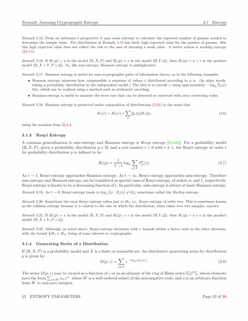
Formally Assessing Cryptographic Entropy 3.1 Entropy
Remark 3.15. From an adversary’s perspective it may seem relevant to calculate the expected number of guesses needed todetermine the sample value. The distribution in Remark 3.12 has fairly high expected value for the number of guesses. Butthis high expected value does not reflect the risk to the user of choosing a weak value. A better notion is working entropy(§3.1.5).
Remark 3.16. If H1(p) = u in the model (Π, X, P ) and H1(p) = v in the model (Π, Y, Q), then H1(p) = u + v in the productmodel (Π, X × Y, P × Q). So, like min-entropy, Shannon entropy is multiplicative.
Remark 3.17. Shannon entropy is useful for non-cryptographic parts of information theory, as in the following examples.
• Shannon entropy measures how compressible a sequence of values x distributed according to p is. (In other words,taking a probability distribution in the independent model.) The idea is to encode x using approximately − log2 Pp(x)bits, which can be realized using a method such as arithmetic encoding.
• Shannon entropy is useful to measure the error rate that can be detected or corrected with error correcting codes.
Remark 3.18. Shannon entropy is preserved under composition of distributions (2.24) in the sense that
H1(r) = H1(r) +X
p
Qr(p)H1(p), (3.6)
using the notation from §2.4.4.
3.1.3 Renyi Entropy
A common generalization to min-entropy and Shannon entropy is Renyi entropy [Ren60]. For a probability model(Π, X, P ), given a probability distribution p ∈ Π, and a real number t > 0 with t 6= 1, the Renyi entropy at order tfor probability distribution p is defined to be
Ht(p) =1
1 − tlog2
∑
x∈X
P tp(x). (3.7)
As t → 1, Renyi entropy approaches Shannon entropy. As t → ∞, Renyi entropy approaches min-entropy. Thereforemin-entropy and Shannon entropy can be considered as special cases of Renyi entropy, of orders ∞ and 1, respectively.Renyi entropy is known to be a decreasing function of t. In particular, min-entropy is always at most Shannon entropy.
Remark 3.19. As t → 0, Renyi entropy tends to log2 |{x : Pp(x) 6= 0}|, sometimes called the Hartley entropy.
Remark 3.20. Sometimes the term Renyi entropy refers just to H2, i.e., Renyi entropy of order two. This is sometimes knownas the collision entropy because it is related to the rate at which the distribution, when taken over two samples, repeats.
Remark 3.21. If Ht(p) = u in the model (Π,X, P ) and Ht(p) = v in the model (Π, Y, Q), then Ht(p) = u + v in the productmodel (Π, X × Y, P × Q).
Remark 3.22. Although, as noted above, Renyi entropy decreases with t, bounds within a factor exist in the other direction,with the bound 1
2H2 6 H∞ being of some interest to cryptography.
3.1.4 Generating Series of a Distribution
If (Π, X, P ) is a probability model and X is a finite or countable set, the distributive generating series for distributionp is given by:
D(p; z) =∑
x∈X
z− log2(Pp(x)). (3.8)
The series D(p; z) may be viewed as a function of z or as an element of the ring of Hahn series Z[[zR]], whose elementshave the form
∑
w∈W awzw, where W is a well-ordered subset of the non-negative reals, and a is an arbitrary functionfrom W to non-zero integers.
§3 ENTROPY PARAMETERS Page 32 of 98

Formally Assessing Cryptographic Entropy 3.1 Entropy
The expression D(p; z) on the left side of (3.8) does not refer explicitly to the probability function P . When itis necessary to distinguish such series for different probability models, a subscript can be used as DP (p; z).
The condition that∑
x∈X Pp(x) = 1 implies that D(p;− 12 ) = 1. The distributive generating series determines
Renyi entropy of order t 6= 1 via
Ht(p) =1
1 − tlog2 D(p, 2−t). (3.9)
Conversely, the Renyi entropies Ht(p) as a function of t determine the distributive generating series D(p; z) as afunction of z.
In a mixed product of two models, as in §2.4.5, a distribution has the form (p, q) where p and q are distributionsin the models over which the product is taken. In this case:
D((p, q); z) = D(p; z)D(q; z). (3.10)
In a common product, a single distribution p is associated with different probability functions, P , Q and R in thenotation of §2.4.5, and
DR(p; z) = DP (p; z)DQ(p; z). (3.11)
Given a distribution p which is known to be an unknown permutation of a common N th power of another unknownbase distribution p from a base model, then taking the N th root of the distributive series of the powered distribution,which can be done using the binomial theorem in the Hahn series formula, the distributive series of the base can bedetermined.
Remark 3.23. Suppose that the cryptographer somehow knows with certainty that a source is governed by a model (Π,X, P )that is some permutation of the (3, 2) independent model for some fixed but unknown permutation. Further suppose that thecryptographer is able to obtain many independent samples from the model (Π, X, P ) and thereby to infer with fairly strongconfidence that the distribution p describing the source satisfies:
x Pp(x)
00 0.11201 0.108902 0.115510 0.115511 0.105612 0.105620 0.11221 0.122522 0.1024
(3.12)
to some approximation. The distributive series for p in the presumed model is then:
D(p, z) = z3.28771 + 2z3.24332 + z3.19892 + 2z3.15843 + 2z3.11404 + z3.02915 . (3.13)
The min-entropy is given by the lowest exponent of the formal terms, which is 3.02915.A more general question is to determine the distribution p. Because the probability model (Π, X, P ) is a permutation of
the (3, 2) independent model, DP (p, z) = DR(p, z)2, where (Π, {0, 1, 2}, R) is the (3, 1) independent model, which is actuallythe unrestricted model on {0, 1, 2}. So, DR(p, z) =
p
D(p, z).Because, R is associated with the (3, 1) independent model, it holds that DR(p, z) = zα + zβ + zγ for some α, β, and γ.
By looking at the symbolic expansion of DR(p, z)2, it can be seen that the values α, β, and γ, can be determined by halvingthe exponents of the terms with coefficient 1 in (3.13).
p
D(p, z) = z1.64386 + z1.59946 + z1.51457. (3.14)
This implies that that p is some permutation of p = (0.35, 0.33, 0.32).
§3 ENTROPY PARAMETERS Page 33 of 98
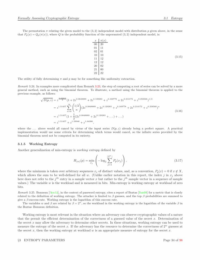
Formally Assessing Cryptographic Entropy 3.1 Entropy
The permutation π relating the given model to the (3, 2) independent model with distribution p given above, in the sensethat Pp(x) = Qp(π(x)), where Q is the probability function of the unpermuted (3, 2) independent model, is:
x π(x)
00 2001 1102 0110 1011 1212 1220 0221 0022 22
(3.15)
The utility of fully determining π and p may be for something like uniformity extraction.
Remark 3.24. In examples more complicated than Remark 3.23, the step of computing a root of series can be solved by a moregeneral method, such as using the binomial theorem. To illustrate, a method using the binomial theorem is applied to theprevious example, as follows:
p
D(p, z) = z3.02915
2 (1 + 2z0.0848889 + 2z0.129283 + z0.169778 + 2z0.214172 + z0.258566)1/2
= z1.51457∞X
n=0
1/2
n
!
(2z0.0848889 + 2z0.129283 + z0.169778 + 2z0.214172 + z0.258566)n
= z1.51457(1 +1
2(2z0.0848889 + 2z0.129283 + . . . ) + . . . )
= z1.51457 + z1.59946 + z1.64386 ,
(3.16)
where the . . . above would all cancel by virtue of the input series D(p, z) already being a perfect square. A practicalimplementation would use some criteria for determining which terms would cancel, so the infinite series provided by thebinomial theorem need not be computed in its entirety.
3.1.5 Working Entropy
Another generalization of min-entropy is working entropy defined by
H(w)(p) = minxj
− log2
⌊2w⌋∑
j=1
Pp(xj)
, (3.17)
where the minimum is taken over arbitrary sequences xj of distinct values, and, as a convention, Pp(x) = 0 if x 6∈ X ,which allows the sum to be well-defined for all w. (Unlike earlier notation in this report, the index j in xj abovehere does not refer to the jth entry in a sample vector x but rather to the jth sample vector in a sequence of samplevalues.) The variable w is the workload and is measured in bits. Min-entropy is working entropy at workload of zerobits.
Remark 3.25. Bonneau [Bon12], in the context of password entropy, cites a report of Boztas [Boz99] for a metric that is closelyrelated to the definition of working entropy. The attacker is limited to β guesses, and the top β probabilities are summed togive a β-success-rate. Working entropy is the logarithm of this success rate.
The variables w and β are related by β = 2w, so the workload in the working entropy is the logarithm of the variable β inthe Boztas–Bonneau definition.
Working entropy is most relevant in the situation where an adversary can observe cryptographic values of a naturethat the permit the efficient determination of the correctness of a guessed value of the secret x. Determination ofthe secret x may allow the adversary to determine other secrets. In these situations, working entropy can be used tomeasure the entropy of the secret x. If the adversary has the resource to determine the correctness of 2w guesses atthe secret x, then the working entropy at workload w is an appropriate measure of entropy for the secret x.
§3 ENTROPY PARAMETERS Page 34 of 98
Formally Assessing Cryptographic Entropy 3.2 Modifications of Entropy
Remark 3.26. One example of this situation arises in typical forms of public key cryptography in which at most one privatekey x corresponds to a given public key, and furthermore, in which it is computationally efficient to test the correspondencebetween the private and public keys. In this case, once the adversary sees the public key, the adversary can use the public keyto efficiently determine the correctness of a guess at the private key.
Remark 3.27. Another example of this situation arises in symmetric-key encryption, where x is the symmetric key, andthe adversary knows, or can reasonably guess, some portion of plaintext, and then sees the corresponding portion of theciphertext. If the length of the known portion of the plaintext is sufficiently long, then the adversary can efficiently determinethe correctness of guesses at the secret.
Remark 3.28. A uniform distribution over a set of size 2h has working entropy h−w bits at a workload of w 6 h bits for eachpositive integer 2w . At workloads of w > h, the working entropy is zero.
Remark 3.29. For any distribution p on a finite (or countable) sample space, H(∞)(p) = 0, so working entropy is zero at infiniteworkload.
Remark 3.30. For a finite sample space H(H0(p))(p) = 0. So, working entropy is zero at a workload equal to the Hartleyentropy.
Remark 3.31. Working entropy is a non-increasing function of w.
Remark 3.32. Consider a bit string x of length 128 with the following nearly uniform distribution. The probability that
x = 0128 is 2−80, and the probability of any other given value of x is 1−2−80
2128−1. This distribution has min-entropy of only 80 bits,
which is 48 bits less than the min-entropy of the uniform distribution on the same sample space. At a workload of 48 bits, theworking entropy of this distribution is about 79 bits, which is only one about bit less than that of the uniform distribution.So, the effect of aberrant spikes in a probability distribution on working entropy is reduced at high workloads.
Remark 3.33. Working entropy, as defined in (3.17), is not a continuous function of w. The following variant is more continuousas a function of w, by adding an extra term to the sum, as follows.
H ′(w)(p) = min
xj
− log2
0
@(2w − ⌊2w⌋) Pp(x⌊2w⌋+1) +
⌊2w⌋X
j=1
Pp(xj)
1
A . (3.18)
Remark 3.34. A remarkable property of Renyi entropies is additivity over (products of) independent distributions (Remarks 3.4and 3.21. Analogously, one can ask if
H(Π,X×Y,P×Q)
(v+w)(p) / H
(Π,X,P )
(v)(p) + H
(Π,Y,Q)
(w)(p)? (3.19)
It is conjectured here that an inequality of such a nature holds.
Remark 3.35. If a bound in the opposite direction to the bound in (3.19) also holds, then assessing the working entropy ofmultiple independent sources might be feasible.
3.2 Modifications of Entropy
This section describes some modified versions of entropy, which are useful to address certain realistic cryptographiccircumstances.
3.2.1 Applied Entropy
In some cryptographic applications, there is a function f : X → Y such that, given a sample value x, only the valuef(x) is used as a key. In this case, the adversary need merely guess f(x). If f(x) is easier to guess than x, then highmin-entropy of x does not suffice for security for f(x).
§3 ENTROPY PARAMETERS Page 35 of 98

Formally Assessing Cryptographic Entropy 3.2 Modifications of Entropy
For example the function f could be: a key derivation function, a hash function, a debiasing function, a uniformityextractor, part of an entropy pooling function, or just a formal way to leave some of the sample x available for otheruse.
A function f : X → Y and a probability model (Π, X, P ) induce the applied model (Π, Y, Q), see §2.4.1 where
Qp(y) =∑
x:f(x)=y
Pp(x). (3.20)
The applied entropy of p in the model (Π, X, P ) under the function f is the entropy of p in the applied model(Π, Y, Q). One can consider applied min-entropy or applied working entropy. The applied min-entropy works out tobe:
Hf(∞)(p) = − log2 maxy∈Y
∑
x:f(x)=y
Pp(x). (3.21)
Remark 3.36. Cachin [Cac97] introduced the notion of smooth entropy. This notion blends the notions of entropy and ran-domness (uniformity) extraction. In the terminology of this report, Cachin considers each function f : X → Y for eachsize of Y , and forms the applied model. Moreover, each applied model is equipped with a metric on the probability space.The smooth entropy is parametrized by some distance value, a smoothness bound in the metrics. The smooth entropy of pat distance d, is the highest entropy of a uniform distribution that is within distance d of an applied distribution obtainedfrom p. Smooth entropy expresses the potential amount of uniform entropy that can be extracted from a source randomness(uniformity) extraction.
In the view of this report, the adversary knows the entropy extraction algorithm. Therefore, the adversary’s ability toguess the applied value is still best described by the applied entropy, not the smooth entropy.
3.2.2 Contingent Entropy
In many cryptographic applications, given a sample value x, there exists some function g such that z = g(x) isrevealed to the adversary. This section defines contingent entropy to address this situation.
Remark 3.37. As an example, suppose that x is modeled by a Markov model, and that a nonce value, such as the initializationvector in the cipher-block chaining mode, is derived from x and sent in the clear. If the nonce does not reveal the whole ofx, then it may still be possible to use x to derive a key. Contingent min-entropy measures the upper possible limit of howsecurely this can be done.
Remark 3.38. One may also assume that there is some side-channel leaking information about x, allowing the adversary tolearn g(x).
First some preliminaries are given. Two functions g : X → Z and f : X → Y are said to be supplementary if thefunction g × f : X → Z × Y : x 7→ (g(x), f(x)) is injective.
Remark 3.39. The intuition is that f(x) provides at least all the information about x that g(x) fails to provide.
The contingent entropy of the distribution p in the model (Π, X, P ) under the condition that the adversary learnsg(x) is the infimum of the applied entropy of p in the applied models (Π, Y, Q) over all f supplementary to g. Onecan consider contingent min-entropy or contingent working entropy.
A function f supplementary to g that seems to minimize entropy (of most types) is the following. Assume thatX is sorted in manner such that Pp is a non-increasing function in the order. Let f(x) be the index of x in the set
§3 ENTROPY PARAMETERS Page 36 of 98

Formally Assessing Cryptographic Entropy 3.2 Modifications of Entropy
g−1(g(x)). This supplementary f induces a model where p has min-entropy:
H∞|g(p) = Hf(∞)(p)
= − log2 maxy∈Y
∑
x:f(x)=y
Pp(x)
= − log2
∑
x:f(x)=1
Pp(x)
= − log2
∑
z∈Z
∑
x:(g×f)(x)=(z,1)
Pp(x)
= − log2
∑
z∈Z
maxx:g(x)=z
Pp(x).
(3.22)
Henceforth, (3.22) will be as taken the definition of contingent min-entropy.
Remark 3.40. Contingent min-entropy coincides with the average min-entropy of Dodis, Ostrovsky, Reyzin and Smith [DORS08].
Remark 3.41. An alternative explanation for (3.22) is that whatever z turns out to be, the adversary will choose the mostlikely x corresponding to that z. So, the sum of maxima represents, over the choice of x, is the probability of the adversarybeing successful.
Remark 3.42. Equations (3.22) with (3.21) differ essentially only in that the maximization and summation operator have beenswapped.
Remark 3.43. Some cryptographic applications, such as public-key cryptography, reveal an injective function f of the privatekey, such as the public key. A similar situation often occurs in symmetric-key cryptography too. For example, when a knownmessage longer than the secret symmetric key is encrypted.
Information-theoretically, the public key determines the private key, and thus leaks all the information. The contingententropy of the key is zero. Fortunately, zero contingent entropy does not mean zero security because the leakage functions inthis case are seem to be one-way functions. It can be said that the private key retains computational contingent min-entropy.
This report does not focus at all computational entropy. This report deliberately focuses on the task of ensuring sufficientinformation-theoretic entropy from noise source, so the entropy can be injected into keys, and the keys can be secret. Thescope of this report is not intended extend further into the keys as they are used.
Such a division scope can be inforamlly justified by the belief that cryptographic algorithms in which the keys are usedare secure. For example, the belief that the function from the the private key to the public key is a one-way function.
Ultimately, the security depends on the combination, but a good heuristic for security may be to analyze the key generationand the key application separately.
Remark 3.44. A definition generalizing information-theoretic and computational contingent entropy may be formulated asfollows. As above, let g be the leakage function, and let f be a function be supplememtary to g. Fix a computational costthreshold t. Define the t-limited contingent entropy as the infimum of the f applied entropy over all f of computational costat most t. As t increases, the t-limited contingent entropy either stays the same or decreases (it does not increase). Threedifferent levels for t may be of interest:
• Set t = ∞. This would be called information-theoretic contingent entropy.
• Set t such that computations of cost t would be infeasible for an adversary. If t = 2s, then s can be called the security
level. Conventionally, this would be called computational contingent entropy.
• Set t much lower, such as to the computational cost of verifying that a guess at key matches the observation (such as apublic key, or a plaintext-ciphertext pair). Call this quick contingent entropy. (One may further qualify quick contingententropy by considering only the best known cost, instead of the best possible cost, which may be unknown.)
Quick contingent entropy is a simple precursor quantity useful for measuring the security of keys before they get used. It isconvenient if it simplifies the assessment of entropy by avoiding the consideration of complicated algorithms. Ultimately, oncekeys are used, in more protocols, their security is limited by computational contingent entropy.
§3 ENTROPY PARAMETERS Page 37 of 98

Formally Assessing Cryptographic Entropy 3.3 Sample-Dependent Entropy Parameters
3.2.3 Contingent Applied Min-Entropy
Let f : X → Y and g : X → Z be functions. Let (Π, X, P ) be a probability model. Suppose that an adversary willlearn z = g(x) and that only f(x) will be used in the generation of a key. The contingent applied min-entropy ofp ∈ Π, under f and g, is defined to be:
Hf(∞)|g(p) = − log2
∑
z∈Z
maxy∈Y
∑
x∈f−1(y)∩g−1(z)
Pp(x). (3.23)
To generalize (3.23) from min-entropy to working entropy of workload w, let the maximization operator be indexedover ⌊2w⌋-element subsets y of Y . An alternative formula for contingent applied min-entropy is as follows:
Hf(∞)|g(p) = − log2 maxα:Z→Y
∑
x:α(g(x))=f(x)
Pp(x). (3.24)
The function α represents the following strategy of an adversary: given z = g(x), guess that f(x) = α(z). Thesum in (3.24) is the probability that the adversary guesses f(x) correctly from z = g(x). The entropy is then thenegative base two logarithm of highest success probability of any adversary. The alternative formula equals theoriginal because:
maxα:Z→Y
∑
x:α(g(x))=f(x)
Pp(x) = maxα:Z→Y
∑
z∈Z
∑
x∈g−1(z)∩f−1(α(z))
Pp(x)
=∑
z∈Z
maxy∈Y
∑
x∈g−1(z)∩f−1(y)
Pp(x).(3.25)
3.2.4 Filtered Entropy
Suppose that (Π, X, P ) is a probability model; and suppose that Y ⊂ X is a subset of the sample space. Supposethat a sample x is drawn from some distribution p ∈ Π. If x 6∈ Y then x is rejected. Otherwise x is accepted. If0 6=
∑
y∈Y Pp(y), then the result is the Y -filtered probability model (Π, Y, Q) as defined by
Qp(y) =Pp(y)
∑
z∈Y Pp(z). (3.26)
The Y -filtered entropy of p is the entropy of p in the filtered model. Explicitly, the filtered min-entropy of distributionp is
(
miny∈Y
− log2 Pp(y)
)
+ log2
∑
y∈Y
Pp(y)
. (3.27)
Remark 3.45. From an implementation perspective, filtered entropy fails to account for the cost of rejecting values of thesource, and it fails to account for the fact that, with some probability, rejection may occur, in which case no entropy isprovided. Arguably, the source could be sampled repeatedly until it is not rejected. This assumes that independent identicallydistributed samples could be obtained. The rate at which entropy is provided would depend on the rate of rejection. Filteredentropy does not depend on the rejection rate.
3.3 Sample-Dependent Entropy Parameters
Sample-dependent parameters are distinct from the previous parameters in that they vary with the sample value.For a probability model (Π, X, P ), a sample-dependent parameter is a function of the form
r : Π × X → R. (3.28)
Sample-dependent parameters can be useful in cryptography when one is assessing the entropy of a value x which isto be used. In other words, in retrospective entropy assessment, sample-dependent parameters may be important.
Remark 3.46. Each of the grading functions from §4 could also be considered as sample-dependent parameters, but these arenot necessarily related to entropy.
§3 ENTROPY PARAMETERS Page 38 of 98
Formally Assessing Cryptographic Entropy 3.3 Sample-Dependent Entropy Parameters
3.3.1 Sample-Entropy (Information Content or Self-Information)
One sample-dependent parameter is the probability function P . It has parameter space R = [0, 1]. This sample-dependent parameter does not have the same units as other entropy parameters, but transforming the parameter byapplying a logarithm, to obtain the parameter I = − log2 ◦P defined by
I(p, x) = − log2(Pp(x)), (3.29)
with the convention that − log2(0) = ∞, yields a sample-dependent parameter with the same units as other notionsof entropy. Previous names for this sample-dependent parameter are information content and self-information. Thisreport shall use the alternative name sample-entropy, emphasizing that it is a type of entropy dependent on thesample.
Remark 3.47. The min-entropy of distribution p is the minimum of the sample entropy I(p, x) over all x ∈ X. Explicitly:
H∞(p) = minx∈X
I(p, x). (3.30)
In particular, sample-entropy is always at least min-entropy: I(p, x) > H∞(p).
Remark 3.48. The Shannon entropy H1(p) of the distribution p is the expected value of I(p, x) for random x ∈ X, distributedaccording to distribution p. Explicitly:
H1(p) =X
x∈X
Pp(x)I(p, x). (3.31)
Remark 3.49. sample-entropy is additive over independent distributions in the following sense. Suppose that (Π, X, P ) and(Π, Y, Q) are models, and that (Π, X × Y, R) is their common product. Then I(p, (x, y)) = I(p, x) + I(p, y). (In a mixedproduct, the additivity would be expressed as I((p, q), (x, y)) = I(p, x) + I(q, y).)
In prospective entropy assessment, sample-entropy cannot be used, because one does not know the sample x, soone cannot compute the sample-entropy. Therefore, the use of sample-entropy is only applicable in retrospectiveassessment. In some cryptographic applications, entropy may be so scarce that one may wish to rely on sample-entropy rather than just min-entropy.
Remark 3.50. The sample-entropy of a bit string can be greater than its length, whereas this is not true for min-entropy orShannon entropy. More generally, sample-entropy can exceed the min-entropy of the uniform distribution.
Remark 3.51. On the one hand, the fact that the sample-entropy can exceed the min-entropy of the uniform distribution makessample-entropy inappropriate for cryptographic applications, because an adversary can always guess the value of x using auniform distribution. On the other hand, when the adversary knows that the distribution is non-uniform, a uniform guess atx is not the adversary’s optimal strategy; so it can still be argued that sample-entropy is meaningful.
Since in this report, the adversary will be assumed to know the inference method of cryptographer, it follows that if thecryptographer is likely to rely on retrospective assessments of sample-entropy that exceed the maximum possible min-entropy,the adversary will be able to predict and choose an alternative strategy.
Remark 3.52. In probability models with sufficiently many probability distributions, the distributions p inferred from thesample x, will generally be such that x is relatively likely under the inferred distribution p. In this case, the inferred sample-entropy might not exceed the min-entropy of the uniform distribution on the sample space. When making inferences withthese models, the difficulties from Remarks 3.50 and 3.51 will not often arise.
Remark 3.53. A general way to view the adversary in the contexts above is as follows. Assume that the adversary knowsthe distribution p of the sample x. The adversary can adopt some probabilistic strategy to guess x, which will described byanother distribution. The adversary’s expected success rate is p · q, thinking of p and q as probability vectors of dimension|X|. Write qx (resp. px) for the probability that distribution q (resp. p) assigns to x. Write q = dx for the distribution q suchthat qx = 1 and qy = 0 for y 6= x.
Let z maximize pz. The min-entropy of p is thus − log2 pz. Four strategies for the adversary and their expected successrates are given below.
§3 ENTROPY PARAMETERS Page 39 of 98

Formally Assessing Cryptographic Entropy 3.3 Sample-Dependent Entropy Parameters
1. Given p, the optimal strategy chooses q = dz. Then the adversary’s expected success rate is p · dz = pz. The negativebase-two logarithm of the success rate with this strategy is the min-entropy of p.
2. If the adversary chooses q = dx, for some other x, then the expected success rate is p ·dx = px. In particular, the negativebase two logarithm of the expected success rate of strategy q = dx is the sample-entropy of x under the distribution p.
3. If the adversary chooses q as the uniform distribution on X, then p · q = 1/|X|. The negative base two logarithm of theexpected success rate is then log2 |X|.
4. If the adversary chooses q = p, then the negative base two logarithm of the expected success rate is the Renyi entropyof order two of the distribution p.
In the event that the sample actually takes the value x, then the adversary’s actual success rate is different from the expectedsuccess rate. In particular, the strategy q = dx has success rate one. But, if nothing about x is leaked, then the adversary hasno information with which to determine this particular strategy.
Remark 3.54. Another potential pitfall of using sample-entropy is that that in distributions p where Pp takes distinct valuesfor every x, the sample-entropy determines x. In this case, if the sample entropy is somehow leaked to an adversary, then theadversary learns x. To avoid a contingent entropy of zero, the sample-entropy must not be leaked.
3.3.2 Eventuated Min-Entropy
Let (Π, X, P ) be a probability model. Let E ⊆ X . Suppose that the event x ∈ E has occurred. Then the eventuatedmin-entropy associated with E is a sample-dependent parameter given by
H∞‖E(p, x) = − log2 maxx′∈E
Pp(x′), (3.32)
for x ∈ E. For x 6∈ E, this parameter’s value does not matter, so it can artificially be set to ∞.
Remark 3.55. The event E in eventuated entropy would generally relate to a partial observation of the sample. For example,if the model is an (m,N) Markov model, and inference is being based on observation of only about N/2 entries of the samplesequence x, then the event E is the set of all x matching the observation initial subsequence.
Remark 3.56. Eventuated entropy is intermediate between min-entropy and sample-entropy. It would be used when theassessment is intermediate between prospective and retrospective.
Remark 3.57. Eventuated min-entropy can be viewed as the sum of filtered min-entropy and applied sample-entropy. Moreexplicitly, given f and y = f(x), the eventuated min-entropy is the sum of the Y = f−1(y) filtered min-entropy and the sampleentropy of the f(x) in the f -applied probability model.
Remark 3.58. Eventuated min-entropy, like min-entropy and sample-entropy, is additive over independent distributions.
3.3.3 Applied Eventuated Min-Entropy
Let (Π, X, P ) be a probability model. Let E ⊆ X . Suppose that the event x ∈ E has occurred. Let f : X → Y bea function, such that only f(x) will be used, say, as part of secret key. Then the applied eventuated min-entropy off(x) associated with E and f is a sample-dependent parameter given by
Hf(∞)‖E(p, x) = − log2 maxy∈f(E)
∑
x′∈f−1(y)
Pp(x′), (3.33)
for x ∈ E. For x 6∈ E, this parameter’s value does not matter, so can be artificially set to ∞.Applied eventuated min-entropy is the eventuated min-entropy of the event y ∈ f(E) in the f -applied model.
§3 ENTROPY PARAMETERS Page 40 of 98

Formally Assessing Cryptographic Entropy 3.3 Sample-Dependent Entropy Parameters
3.3.4 Contingent Eventuated Min-Entropy
Let (Π, X, P ) be a probability model. Let E ⊆ X . Suppose that the event x ∈ E has occurred. Let g : X → Z be afunction, such that g(x) will be learned by an adversary. Then the contingent eventuated min-entropy of x associatedwith E under leakage of g(x) is a sample-dependent parameter given, for x ∈ E, by
H∞|g‖E(p, x) = minf :X→Y
Hf(∞)‖E(p, x), (3.34)
where f ranges over all function supplementary to g (see §3.2.2). For x 6∈ E, this parameter’s value does not matter,so can be artificially set to ∞.
§3 ENTROPY PARAMETERS Page 41 of 98

Formally Assessing Cryptographic Entropy
4 Statistical Inference
Formally assessing cryptographic entropy involves making a statistical inference, which is defined in this section. Instatistical inference: the probability model is given; a sample is observed; and then something about the distributionis inferred. So, the known input variables to an inference problem are the model (Π, X, P ) and a sample x ∈ X . Theunknown variable is the distribution p. In cryptography, it is mainly important to infer something about the certainparameters of the distribution p, specifically the entropy parameters defined in §3.
For an inference to be reasonable, the general idea is to infer, from an observed sample x, a set of distributionsp from the given probability model that meet some set of criteria for consistency between p and x. In cryptographicapplications, when inferring an entropy parameter from the set of inferred distributions, it is prudent to take theleast entropy parameter of the inferred distributions.
Remark 4.1. Inference necessarily involves guessing, because x generally gives incomplete information about p. There may bemany different distributions p ∈ Π consistent with x in the sense that Pp(x) 6= 0, and it is not strictly possible to know whichof these p is the correct. So inference is imperfect.
Remark 4.2. Because of the intrinsic imperfection and incompleteness of inference, an inference method can at best be rea-sonable, not perfect. Reasonable is perhaps definable, but it will not be formally defined it in this report. Instead, examplesof some inference method are given. This report contends that these methods are generally reasonable.
Remark 4.3. In this report, the view is taken that, to be reasonable, an inference method must at least be well-defined onall, or a very large class, of probability models. In this section, inference methods are generic in the sense that they aredefined in terms of an arbitrary discrete probability model. Furthermore, a reasonable inference method should not just bewell-defined, but should also agree with intuition on simple models. The inference methods defined in this section are all basedsolely on comparing probabilities, and should therefore be reasonable as inference methods, and also appropriate for use incryptography.
Remark 4.4. The generic inference methods defined in this section are invariant under isomorphism of models. For somemodels, the generic inference methods are ineffective, essentially because the model has too many isomorphisms. To addressthis situation, sample statistics, see §5, can be used. Sample statistics induce another model, generally with fewer isomorphisms,upon the generic inference methods can be applied more effectively.
4.1 Inference functions
An inference function for (Π, X, P ) is a function that takes input of X and outputs some assertion about the unknowndistribution p. In this report, three types of direct assertions about p are considered. Later, it will be discussed howsuch inferences about p may be converted into inferences about the cryptographically important parameters of p.
4.1.1 Point-valued inferences
An inference function i for model (Π, X, P ) is point-valued if it is a function of the form i : X → Π. That is, to eachsample value x it assigns a probability distribution, which can be called the inferred distribution.
4.1.2 Set-valued inferences
Let (Π, X, P ) be a probability model. Let [Π] be the set of all subsets of Π. An inference function for model (Π, X, P )is set-valued if it is a function of the form i : X → [Π]. That is, to each sample value x it assigns a set of distributions,which is called the inferred set of distributions, or the set of inferred distributions.
Remark 4.5. Generally, set-valued inference functions should respect equivalence of distributions: if p ∈ i(x) and p ≡ q, thenq ∈ i(x). Otherwise, the set-valued inference functions should be deemed unreasonable.
Remark 4.6. In this report, several specific set-valued inference functions will be considered.
§4 STATISTICAL INFERENCE Page 42 of 98

Formally Assessing Cryptographic Entropy 4.1 Inference functions
Remark 4.7. Often, the inferred sets contain just a single distribution. In such cases, the set-valued inference acts like point-valued inference. Sometimes a sample value x ∈ X has an inferred set containing many distributions, even infinitely many.For such a sample, a set-valued inference function is unable to prefer one distribution over the other in the inferred set. Forcryptographic applications, the most cautious choice of distribution can be inferred, as described in §4.5.2.
Remark 4.8. The inferred set is sometimes empty.
4.1.3 Grading-valued inferences
A grading on the model (Π, X, P ) is a function g : Π → [0,∞), meaning a non-negative real-valued function on theprobability space. The set of gradings can be written Γ(Π).
A strict grading is a function g : Π → [0, 1]; so a strict grading takes value at most one. Usually, the gradingsconsidered in this paper will be strict gradings. The set of strict gradings can be written [0, 1]Π.
A binary grading is function g : Π → {0, 1}; so a binary grading is a strict grading taking only integer values.The set of binary gradings can be written {0, 1}Π. A binary grading can be regarded as equivalent to a subset of Πby the relation g ≡ g−1(1).
A grading-valued inference function for model (Π, X, P ) is a function of the form i : X → Γ(Π); so i assignseach sample value x a grading g = i(x) of all probability distributions in the probability space Π. The intentionof a grading-valued inference function is that a higher value of the inferred grading is intended to indicate betterconsistency of the sample value x the distribution p.
Remark 4.9. Generally, grading-valued inference functions should respect equivalence of distributions: if g = i(x) is an inferredgrading function and p ≡ q, then g(p) = g(q).
If i(x) = g, then g(p) is called the grade of p at x. In strict notation, the grade is i(x)(p), but to avoid the doubleargument, the notations i(x, p) or even ix(p) may be used when clear from context. So, a grading-valued inferencefunction may be thought of as a bivariate function i : X × Π → [0,∞). With a slight re-use of terminology, such abivariate function will also be called a general grading function. So, a grading-valued inference function determinesa general grading function, and vice versa.
Remark 4.10. For a fixed probability distribution p and a grading-valued inference function i, a function ip : X → [0, 1] : x 7→i(x, p) can be defined. So, if i(x) = g, then ip(x) = g(p).
Remark 4.11. Unlike probability functions, there is no requirement that the grading function g : Π → [0, 1] sums to one overΠ, in the sense that
P
p∈Π g(p) = 1 if, say, Π is finite. Indeed, in general, for infinite probability spaces (for which no measurehas been assigned), such summation to one is not even a well-formulated requirement. If Π is equipped with a measure, itmay be convenient for g to be a measurable function, ideally whose total integral over Π is finite.
Remark 4.12. The output of a grading-valued inference function for a probability model with infinite probability space describesan infinite amount of information (but will typically be described with a finite formula). For the purposes of cryptography, whatis needed is a single estimate of entropy, a single real number, or perhaps even just a single bit: a decision to accept or reject.As such, grading-valued inference functions seem not to be immediately usable for cryptographic applications. Nevertheless,other inferences may be derived from grading-valued inference functions. For example, graded set-valued inferences are derivedfrom grading-valued inferences. So, it will turn out that grading-valued inference functions can serve as intermediate steps incryptographic applications.
4.1.3.1 Expectation of General Gradings It can be informative to consider the expected value of a generalgrading function g : X × Π → [0,∞), at a given probability distribution. Precisely, this is defined as
Eg(p) =∑
x
g(x, p)Pp(x). (4.1)
The value Eg(p) gives a way to calibrate a grading value g(x, p), especially if p has been inferred from x using thegrading g. If g(x, p) is many magnitudes lower than Eg(p), then one may even infer that the probability model itselfis not accurate.
§4 STATISTICAL INFERENCE Page 43 of 98

Formally Assessing Cryptographic Entropy 4.2 Inference Methods
Remark 4.13. For the likelihood grading, §4.4.1, EgL(p) =
P
x Pp(x)2. For the uniform distribution, and more generally,distributions with high min-entropy, this value can be quite low. In fact, taking the negative logarithm of the expectedlikelihood grading gives − log2(EgL
(p)) = H2(p), the Renyi entropy of order two. The Renyi entropy of order two is known tobe at most twice min-entropy. So, for high entropy sources, the expected likelihood can be quite small.
Remark 4.14. For typicality grading, §4.4.2,
Egk(p) =
X
x
gk(x, p)Pp(x)
=X
Pp(y)<Pp(x)
Pp(y)Pp(x) + kX
Pp(y)=Pp(x)
Pp(y)Pp(x)
=1
2
0
@
X
Pp(y)<Pp(x)
Pp(y)Pp(x) +X
Pp(y)>Pp(x)
Pp(y)Pp(x) + 2kX
Pp(y)=Pp(x)
Pp(y)Pp(x)
1
A
=1
2
0
@
X
x,y
Pp(y)Pp(x) + (2k − 1)X
Pp(y)=Pp(x)
Pp(y)Pp(x)
1
A
=1
2
0
@
X
x
Pp(x)
!2
+ (2k − 1)X
Pp(y)=Pp(x)
Pp(x)2
1
A
= 12
+ (k − 12)X
x
Pp(x)2Qp(x),
(4.2)
where Qp(x) is the number of y such that Pp(x) = Pp(x).Therefore, the expected value of the balanced typicality is exactly one half. Inclusive typicality averages to more than one
half, and exclusive to less. If Pp takes distinct values for all x, then the expected inclusive and exclusive typicality differ fromone half by the expected value of the likelihood grading. If p is a uniform distribution, then the expected value of inclusivetypicality is one: indeed inclusive typicality is one: all values of x are equally typical. Conversely, the expected value ofexclusive typicality is zero for a uniform distribution p.
Therefore, inclusive and balanced typicality are inherently calibrated in the sense that, no matter what p is, the expectedtypicality is at least one half. Furthermore, if x is such that g1(x) ≪ 1
2or g1/2(x) ≪ 1
2for probability distributions p in the
probability model, then one can infer from x that perhaps the probability model is not valid.
Remark 4.15. The expected value of all generalized typicalities, see §4.4.3, are 12.
Remark 4.16. The expected value of the Bayesian grading §4.4.6 is
EB(p) =1
R
ΠLxdµ
X
x∈X
Pp(x)2, (4.3)
and is a scaled version of the expected value of the likelihood grading.
4.2 Inference Methods
An inference method is a function that takes a probability model (Π, X, P ) and outputs an inference function for(Π, X, P ). An inference method is point-valued if all inference functions it produces are point-valued. Similarly, aninference method is set-valued if it only outputs set-valued inference functions, and grading-valued if it only outputgrading-valued inference functions.
Remark 4.17. A grading-valued inference method I is a function to functions to functions: on input of a probability model(Π, X, P ), the inference method I outputs a grading-valued inference function i, which, in turn, is a function with domain Xand range of functions from Π to [0, 1].
A grading-valued inference function for the probability model (Π, X, P ) has an associated general grading functiong : X × Π → [0, 1]. Any function that maps a model to such a general grading function on the model is called a
§4 STATISTICAL INFERENCE Page 44 of 98
Formally Assessing Cryptographic Entropy 4.3 Set-Valued Inference From Grading-Valued Inferences
general grading method. Each grading-valued inference method defines a general grading method, and each generalgrading method defines a grading-valued inference method.
4.3 Set-Valued Inference From Grading-Valued Inferences
In this section, two ways to derive a set-valued inference method from a grading-valued inference method are given.Collectively, such methods graded inference methods are called in this report.
4.3.1 Maximally Graded
Suppose that g is a general grading on model (Π, X, P ), associated with a grading-valued inference function ig. Themaximally graded inference associated with grading g is a set-valued inference imax g function defined as follows:
imax g(x) = {p : g(x, q) 6 g(x, p)∀q ∈ Π} . (4.4)
Graded inference imax g may be thought of as derived from g or from ig.
Remark 4.18. In some cases g is discontinuous and as such a maximum p may not exist. In these cases, an alternativedefinition may sometimes be available. Consider the supremum of gradings values at x, written sx = supp∈Π g(x, p). Definesets Sǫ = {p : g(x, p) > sx − ǫ} ⊆ Π, which are nested according to the size ǫ.
As a matter of convenience, define the following. Let Sǫ be the closure of Sǫ in some natural topology on Π. If isup g(x) =T
ǫ>0 Sǫ is non-empty (which is true if Π is given a compact topology), it may serve as a suitable substitute for an empty setimax g(x), even if values of g(x, p) < sx for p ∈ isup g(x).
In cryptographic applications, it is in entropy parameters, not the distributions themselves, that are most important.If the parameters are continuous then the definition of isup g(x) above will provide the desired answer for the parameters.For discontinuous parameters isup g(x) may not be what is desired. In this case, isup g(x) should be thought of, not as theintersection of the chain of sets of Sǫ, but rather as the limit of the chain of sets Sǫ. This enables us to consider limits ofparameters on Sǫ, which may differ from the value of parameters on the intersection.
Remark 4.19. In many cases, the inferred set imax g(x) is a single element (singleton) set. In this case, the inference is muchlike a point-valued inference function. However, there are often some values of x for which several, possibly infinitely many,different distributions p attain the maximal value.
If G is a general grading method or IG is grading-valued inference method, then it is possible to derive a set-valuedinference method Imax G using the inference functions above.
Remark 4.20. Maximally graded inferences are model-dependent in the sense that definition (4.4) includes Π. A potentialconsequence of this model-dependence is that the maximally graded inference in the restriction (Θ, X, P ) of the model (Π, X, P ),may not have a given relation with the maximally graded inference in the model (Π, X, P ).
4.3.2 Threshold Graded and Confidence Levels
Suppose that g is a general grading on a model (Π, X, P ). Let t ∈ [0, 1] and call this value the threshold level. Thethreshold graded inference function ig>t is a set-valued inference function defined by
ig>t(x) = {p : g(x, p) > t}. (4.5)
If t > u, then ig>t(x) ⊆ ig>u(x), so the sets obtained are shrinking or stable in size as a function of the threshold.A high threshold may lead to a narrow, perhaps even empty, inference, while a low threshold may lead to a broadinference.
The value c = 1 − t may sometimes be called the confidence level of the inference. As confidence increases, thebreadth of the inference may increase (or stay stable). This reflects the intuitive notion that one can generally makethe sacrifice of broadening the inference set in order to gain a more confidence in the inference. Gradings are bestsubjected to a threshold when the distribution of the grading, for fixed p and varying x, has some resemblance to theuniform distribution on [0, 1], because then the confidence level has more meaning. In the following sections, somegradings will have such a property, and others will not.
§4 STATISTICAL INFERENCE Page 45 of 98
Formally Assessing Cryptographic Entropy 4.4 Example Gradings
Remark 4.21. Threshold graded inferences are not model-dependent in the sense of Remark 4.20 provided that the grading isnot model-dependent. In particular, if the iΘ(x) is threshold graded inference in the model (Θ,X, P ) that is a restriction ofthe model (Π,X, P ), and iΠ(x) is the threshold graded inference in the model (Π,X, P ), then
iΘ(x) = Θ ∩ iΘ(x). (4.6)
When using such a threshold graded inference and taking the infima of parameters, as in §4.5.2, then restriction of the modelcannot decrease the inferred parameter, and relaxing model cannot increase the inferred parameter.
Remark 4.22. As noted in Remark 2.5, it may sometimes be possible that an adversary can influence the choice of p inΠ. If an adversary has such power over p, then a maximally graded inference has little value. For appropriate gradings, ahigh-confidence threshold grading would still have some value.
4.4 Example Gradings
In this section, some generic and reasonable grading methods are given.
4.4.1 Likelihood
The likelihood grading gL is defined bygL(x, p) = Pp(x). (4.7)
For convenience, the associated inference function may also be written as Lx = igL(x) in this report. Therefore
Lx(p) = Pp(x).The term likelihood, instead of probability, is used here to avoid thinking that Lx has the properties of a probability
function. For example, summing (or integrating) the values of Lx over all probability distributions is not guaranteedto yield 1.
Remark 4.23. For likelihood, an exception will be made here about the general grading’s name. Since the general grading isalso the probability function, the grading will be the likelihood grading to avoid confusion with the probability function in itsusual role.
Remark 4.24. Likelihood is, of course, a well-known and fundamental notion in statistical inference.
4.4.2 Typicality
For a given inclusivity level k ∈ [0, 1], define the typicality grading gk as follows:
gk(x, p) =
∑
y:Pp(y)<Pp(x)
Pp(y)
+ k
∑
y:Pp(y)=Pp(x)
Pp(y)
. (4.8)
In this report, the only k that will be considered are k ∈ {0, 12 , 1}, which give rise to exclusive, balanced and inclusive
typicality, respectively.
Remark 4.25. Inclusive typicality g1(x, p) is the probability that a random sample y is at most as probable as x. Exclusivetypicality g0(x, p) can also be defined as the probability that a random sample y is less probable than x. Balanced typicalityis the average of inclusive and exclusive typicality, in other words, it is half-way between inclusive and exclusive.
Remark 4.26. Typicality, unlike likelihood, when used for inference, attempts to capture the notion of how a sample comparesin probability to other samples under the same probability distribution. This notion was used in the intuitive reasoning forthe loose inference in §1.1.2.8, where it was argued that 210-uniform was not to be inferred, because more repetitions wouldhave been expected in the sample.
Remark 4.27. For a fixed distribution p, ranking sample values x by typicality or likelihood gives the same ranking. For fixedx, and varying p, the rankings induced by typicality may differ from those by likelihood.
§4 STATISTICAL INFERENCE Page 46 of 98

Formally Assessing Cryptographic Entropy 4.4 Example Gradings
Remark 4.28. When p is a uniform distribution on X, then typicality is constant for all x, and takes on the value k, theinclusivity. When p is an almost uniform distribution on X, then for the most probable x, it takes value approximately1 − (1 − k)/|X|. For k < 1, this will be larger than the typicality at the uniform distribution.
Remark 4.29. When p is subuniform on X, then
gk(x, p) =
(
k if Pp(x) > 0
0 if Pp(x) = 0.(4.9)
As such, in models that admit subuniform distributions, any inference based on typicality treats them equally. This effectmay be summarized as: subuniform distribution have tied typicality. This is called the tying effect in this report.
Some models may admit distributions with higher typicality than all subuniform distributions, in which case some usefulinferences can be made. In some cases, sample statistics (§5) may serve as tiebreakers between subuniform distributions.
Remark 4.30. Inclusive typicality is always at least as large as likelihood:
g1(x, p) > gL(x, p), (4.10)
but balanced and inclusive typicality could be less. Similarly, 1 − g0(x, p) > gL(x, p). A stronger fact is that the gap betweenexclusive and inclusive typicality is always at least the likelihood.
g1(x, p) − g0(x, p) > gL(x, p). (4.11)
Remark 4.31. The notion of typicality is based on well-known notions in statistics of significance level, p-value (also knownas percentile or quantile, depending on the units) and cumulative probability function. The general notion of significance level
refers to a value of the p-value. The general notion of p-value is a sample statistic (see §5) that has a uniform distribution on[0, 1], at least under the null hypothesis.
A p-value statistic may be formed for continuous distributions by taking a cumulative probability function with respect tosome function f defined on the sample space. Any choice of function f yields a p-value. So, the p-value of x is the probabilitythat f(y) 6 f(x), for y drawn from the same distribution. A common use of p-values occurs when the distribution is a normaldistribution and the function f is the identity, then p-value is related to the Gauss error function.
In cryptographic applications, distributions are typically discrete, so achieving a proper p-value uniformly distributed in[0, 1] cannot be strictly guaranteed. Typicality only approaches a uniform distribution.
In cryptographic applications, the parameters of interest, entropy and so on, depend primarily on the distribution, not onspecific properties of the structure of x. Typicality is the cumulative probability with respect to the probability function.
Remark 4.32. Typicality ranks the sample space by probability. Such a ranking is often implicit in rankings of popularity,such as sales charts and election results.
Remark 4.33. For an almost uniform distribution (with no equal probabilities), the distribution typicality is almost uniformlydistributed in [0, 1], much like a p-value.
Remark 4.34. Randomized typicality g?(x, p) is a random variable defined with the same equation (4.8) as typicality, exceptthat the variable k is selected uniformly at random from the interval [0, 1]. If the distribution of p is fixed, and x has theprobability distribution given by p, then g?(x, p) is uniformly distributed in [0, 1].
Remark 4.35. The notion of typicality adapts the notion of significance level towards the task of assessing min-entropy, in thatit ranks the samples according to their probabilities.
4.4.3 Generalized Typicality and Adjusted Likelihood
Let σ : [−1, 1] → [−1, 1] be an odd, non-decreasing function.
Remark 4.36. Odd means that σ(−x) = −σ(x) and non-decreasing means that if x < y then σ(x) 6 σ(y).
Remark 4.37. Write σ(x) = xf(x2), where f : [0, 1] → [0,∞) as a function such that for x > 0, it holds that f(x) < 1/√
x.
§4 STATISTICAL INFERENCE Page 47 of 98

Formally Assessing Cryptographic Entropy 4.4 Example Gradings
Generalized typicality is parametrized by the function σ. Generalized typicality parametrized by σ is calledσ-typicality and is defined by
tσ(x, p) = 12
(
1 +∑
y
Pp(y)σ (Pp(x) − Pp(y)) .
)
. (4.12)
This is a generalization of balanced typicality in the following senses.
1. Putting σ(x) = x/|x| for x 6= 0 and σ(0) = 0, which is to say, putting σ(x) equal to the sign of x, thenσ-typicality is balanced typicality.
2. For any σ meeting the stated conditions, σ-typicality is bounded, like balanced typicality, such that tσ(x, p) ∈[0, 1] for all x and p. (This is due to the values of σ belonging to [−1, 1].)
3. The expected value (see §4.1.3.1) of σ-typicality is 1/2, just like balanced typicality. (This is due to σ beingan odd function.)
Remark 4.38. When p is subuniform on X, then
tσ(x, p) =
(
12
if Pp(x) > 012− σ(Pp(y))
2if Pp(x) = 0 and Pp(y) > 0.
(4.13)
As such, in models that admit subuniform distributions, any inference based on generalized typicality treats all subuniformdistributions equally. In such cases, sample statistics (§5) may serve as tiebreakers.
Remark 4.39. For threshold-graded inference at confidence levels of 12
or higher, all subuniform distributions in the modelmust be considered, because of the upper case in (4.13).
Remark 4.40. For threshold-graded inference at confidence levels strictly higher than 12, given sample x, some subuniform
distributions p in which Pp(x) = 0 may be inferred, because of the lower case of (4.13). Call this an aberrant inference.Aberrant inferences can be viewed as a strong discrepancy with the likelihood grading.
Balanced typicality does not exhibit aberrant inferences because the σ is the sign function, which causes the lower termto be zero in the lower case of (4.13).
Despite aberrant inferences, generalized typicality can still be useful for assessing entropy. For example, at a givenconfidence level, only those subuniform distributions among those allowed within the probability model, with a support of agiven size but not containing the given sample x will be inferred.
If the infimum entropy is always attained at an aberrantly inferred subuniform distribution, then at least the inferredentropy decreases with confidence level, decreasing to 0 as the confidence level approaches 1.
Remark 4.41. Generalized typicality sheds some light on a potential difficulty of balanced typicality: its discontinuity. Thediscontinuity is made clearly attributable to the discontinuity of the sign function σ when viewed of as a case of generalizedtypicality.
Balanced typicality has the disadvantage of being discontinuous, which can make bounding and optimizing balancedtypicality difficult. This disadvantage can perhaps be overcome by using the observation that balanced typicality isσ-typicality with σ equal to the sign function. The idea is then to use an alternative σ function, which is continuous,or even smooth, but still similar enough the sign function to so that the resulting σ-typicality inherits the desiredproperties of balanced typicality.
The simplest continuous form of generalized typicality is given by the choice σ1(x) = x. In this case, formula (4.12)simplifies to:
tσ1(x, p) = 12
(
1 + Pp(x) −∑
y
Pp(y)2
)
. (4.14)
As a function of x, with p fixed, the varying term in the sum, 12Pp(x), is a scaling of the likelihood grading. When p
varies, the term∑
y Pp(y)2 varies, but independently of x. This special case of generalized typicality will be calledadjusted likelihood.
§4 STATISTICAL INFERENCE Page 48 of 98
Formally Assessing Cryptographic Entropy 4.4 Example Gradings
Remark 4.42. Adjusted likelihood can be related to order-two Renyi entropy by tσ1(x, p) = 12
“
1 + Lx(p) − 2−H2(p)”
.
Remark 4.43. Adjusted likelihood, and other generalized typicalities, can, for certain distributions p, even distributions mod-erately distant from uniform distributions, be very close to 1
2, for two reasons. First, both the likelihood and adjustment terms
can be quite small even for quite non-uniform distribution. Second, the difference between the likelihood and the adjustmentterm can very small. Calculations done with such typicalities may require considerably high degrees of precision.
Adjusted likelihood may also be expressed as
tσ1(x, p) = 12
54 −
(
Pp(x) − 12
)2 −∑
y 6=x
Pp(y)2
(4.15)
which is an affine transformation of the square of the Euclidean distance (as would be natural to define in theunrestricted model) between the distribution p and the pseudo-distribution hx that has probability 1/2 of takingvalue x, and probability 0 otherwise. So, tσ1(x, p) = 5
8 − 12‖hx − p‖2.
Two other families of σ, generalizing σ1, seem reasonable to consider.
1. Let σ1/m(x) = m√
x for m odd. At m = 1, the function is σ1(x) = x, which gives the adjusted likelihood, asalready seen. Taking m → ∞, these functions approach the sign function. These functions σ1/m are continuous,but have infinite slope at 0, which may make some optimization algorithms difficult.
2. Let
σm(x) = x
m−1∑
n=0
(−1/2
n
)
(x2 − 1)n, (4.16)
for integers m > 1. At m = 1, the function is σ1(x) = x (and is the same as σ1(x) above). As m → ∞, thefunctions approach the sign function.
Remark 4.44. The series (4.16) comes the from the Taylor series expansion of 1/√
x at x = 1, and using polynomial prefixesof these series as a function f(x) and defining σ = xf(x2).
Remark 4.45. The function σ2(x) = x2(3 − x2). The function σ3(x) = x
8(15 − 10x2 + 3x4). Also, σ′
m(0) = O(√
m) seems to
hold, with 2p
m/π seeming to be a good approximation.
In generalized typicality, summation over all y results in some symmetry. For example, taking the polynomials σm
above, we can write:
tσm(x, p) =
m−1∑
n=0
Qn(p)Pp(x)n, (4.17)
where Qn(p) is a symmetric polynomial evaluated at all of the variables Pp(y) (for each possible value of y). ExpressingQn(p) as a polynomial of symmetric polynomials, such as elementary symmetric polynomials, may give a sum withfewer terms than there are values of y, and as such, may make calculating with and optimizing σ-typicality easier.
Remark 4.46. In the independent model, Qn(p) can also be expressed as a related symmetric function of the components ofthe p vector.
4.4.4 Calibrated Typicality
Generalized typicality tσ may have a tendency to be too close to 12 , and as such be not too useful for establishing
confidence levels. For a grading to be most meaningful in the sense of confidence levels, the distribution of thegrading should be somehow nearly uniform on the interval [0, 1]. More precisely, for each fixed p, the distributiong(x, p) should be almost uniform.
Balanced typicality and generalized typicality approach such uniformity mainly in the sense that g has expectedvalue 1
2 and g is value within [0, 1]. Another measure of closeness to uniformity that could be used is the variance.
§4 STATISTICAL INFERENCE Page 49 of 98
Formally Assessing Cryptographic Entropy 4.4 Example Gradings
The variance of the uniform variable in [0, 1] is 112 . So given a grading g with expectation 1
2 and variance v, onecould apply a linear transformation to get another grading g′ = 1
2 + 1√12v
(g − 12 ), with expectation 1
2 and variance112 . A potential problem with g′ is that it might have value outside the range [0, 1], in which confidence levels makelittle sense (a negative confidence level or confidence level higher than 1 makes little sense).
An alternative calibration method is as follows. Let κ : [0, 1] → [0, 1] be another odd function. Then κ-calibratedσ-typicality is defined to be:
tσ,κ(x, p) = 12
(
1 + κ
(
∑
y
Pp(y)σ(Pp(x) − Pp(y))
))
. (4.18)
Balanced typicality is the special case of calibrate typicality in which κ is the identity function and σ is the signfunction.
4.4.5 Agreeability Gradings
The notion of statistical distance from (2.29), which has sometimes been used in cryptography, can be adapted toact like a grading. Let px be the deterministic distribution, in the unrestricted model, that takes on sample value xwith probability one, and thereby all other values with probability zero. One could define the agreeability gradingas
ga(x, p) = 1 − d(px, p), (4.19)
but such an agreeability grading simplifies to
ga(x, p) = Pp(x), (4.20)
which is just the likelihood grading.One could use other distance metrics, such as those based on the Euclidean metric (L2 norm), as defined on the
natural parametrization of the unrestricted model, In fact, adjusted likelihood is already related to such a metric.One could also use a distance based on the L∞ norm to define an agreeability rating.
4.4.6 Bayesian Grading and Posterior Probabilities
The Bayesian grading Bx : Π → [0,∞] can be defined when the probability space Π is equipped with a measure µ,and the likelihood grading Lx is measurable and integrable with respect to this measure. It is defined as:
Bx =Lx
∫
Π Lxdµ. (4.21)
Also write Bx(p) = B(x, p), where convenient.
Remark 4.47. The Bayesian grading is based on Bayes’ law for conditional probabilities. Elaborating the probability notationslightly (to a notation so commonly used in much previous work that formal definitions will be omitted in this report), Bayes’law states that the conditional probability is P (A|B) = P (A ∩ B)/P (B). This implies that P (B|A) = P (A|B)P (B)/P (A).For the problem at hand, the conditional probability, P (p|x), of the hypothesis p given the evidence x is wanted. This isgiven by the formula P (p|x) = P (x|p)P (p)/P (x). The factor P (x|p) = Pp(x) = Lx(p), by definition. The factor P (x) is themarginal probability of x over all possible distributions p, using the associated prior probabilities, which is the integral in thedenominator of (4.21). The factor P (p) is set to 1 in (4.21) because it is really covered by the measure µ itself. In otherwords, when integrating the function Bx over the measure, the measure provides the contribution of P (p), that is, the priorprobabilities.
Remark 4.48. Define ν = Bxµ as another measure on Π with the definition ν(S) =R
SBxdµ for any subset S ⊆ Π. In fact,
this resulting measure satisfies ν(Π) = 1, so actually ν can be used to define probabilities of the probabilities distribution.These are known as the posterior probabilities.
§4 STATISTICAL INFERENCE Page 50 of 98

Formally Assessing Cryptographic Entropy 4.5 Parameter Inference
4.5 Parameter Inference
Cryptographers are primarily interested in inference about the entropy parameters.
4.5.1 Converting Distribution Inference from Parameter Inferences
If i is an inference function for a model (Π, X, P ) and r : Π → R is a parameter on the model, then it is sometimespossible to define an indirect inference function for R, which is a function from X to assertions about R. Thedefinition depends on the nature of the inference function, as given below.
4.5.1.1 Point-valued For a point-valued inference function i : X → Π, the naturally parameter induced inferencefunction for R is defined as j : X → R : x → r(i(x)).
4.5.1.2 Set-valued For a set-valued inference function i mapping X to subsets of Π, the naturally parameterinduced inference function j for R maps X to subsets of R in the following manner. For T ⊆ Π, define r(T ) = {r(p) :p ∈ T } and define j(x) = r(i(x)).
4.5.1.3 Grading-valued For a grading-valued inference function i mapping X to functions from Π to [0, 1], thenthere is no naturally induced inference function for R, unless further information is available. If the probability spaceis equipped with an appropriate measure, define the Bayesian parameter induced inference function j : R → [0, 1], asfollows. For y ∈ R, let j(y) be the average value of i over the subset r−1(y) of the probability space Π. The functionj is only defined where the sets r−1(y) are measurable and where i is measurable on this set.
4.5.2 Narrowing Set-Valued Entropy Inferences to a Point-Valued by Infima
Often, a narrower inference is desired than provided by a set-valued naturally parameter induced inference. In thiscase, one may want to apply a further function to the parameter inference j(x). For example, if the parameter spaceR is an ordered set, then one can take the minimal (or infimum) value of r on the set j(x).
In cryptography, one wants to be prudent, so taking a minimum, or infimum, value of min-entropy over a set ofreasonably inferred possible probability distributions is best.
Remark 4.49. By contrast, when statistical inference is applied to the natural sciences, prudence may indicate the opposite:when narrowing a wide inference one may should opt for the inferred distribution(s) with the highest entropy. Both casesuse the concept of assuming the worst case. In natural sciences, the worst case is the most unpredictable distribution, but incryptography the worst case for the generator of a key, the worst case is the most predictable distribution.
This discrepancy may formally result dangers of using conventional statistics to assess cryptographic entropy. In conven-tional statistics, the models (and sample statistics) may be restrcted in a way a that has little effect if the restriction mainlyremoves distributions of low entropy that the worst-case-narrowing of inference described above would never infer. Indeed, itmay be the case that in natural sciences, models are pre-selected in this manner, so that any formal narrowing of inference isunnecessary.
On the other hand, one does not want to waste entropy when it is scarce, so one needs to strike a balance. Tothis end, one may want to isolate conceptually the stage where one might underestimate entropy, specifically to thisstage. In particular, if the inferred set of entropies includes both large and small values, perhaps application of asecond inference method is appropriate.
Remark 4.50. In the case of a Bayesian parameter induced inference function j where the parameter space R is also equippedwith a measure, then one can take the weighted average of parameter values in the parameter space R using the function j asthe weighting.
In general averaging is risky in cryptography because adversaries are not restricted to average behavior, so this method isnot recommended for estimating min-entropy in cryptography.
§4 STATISTICAL INFERENCE Page 51 of 98

Formally Assessing Cryptographic Entropy
5 Sample Statistics
A sample statistic, or just a statistic, on a probability model (Π, X, P ) is a function s : X → S, where S is someset called the statistic space. A statistic method is a function from probability models to statistics on these models.More precisely, a sample statistic refers to function s : X → S, only when it is used to make an induced inference asdefined in §5.2.
A reason to make induced inferences with sample statistics is that, sometimes, the tying effect from Remark 4.29causes the methods of §4, if applied directly, to yield unsatisfactory inferences.
Remark 5.1. An inference function §4.1 and a sample statistic are both functions with a domain being the sample space. Aninference function can therefore be used as a sample statistic, see Remark 5.8.
Remark 5.2. A induced inference using a sample statistic, which is well-known in cryptography, is the runs test. A uniformmodel is hypothesized for some purported random bit string. The number of runs, which is the sample statistic, is computedfor the string. This number is compared to the distribution of the number of runs for a uniformly random bit string. If thenumber of runs is too low or too high, the uniform model is rejected. Although this is an instance of hypothesis testing, samplestatistics can be also be used in entropy assessment.
5.1 Induced Model
A statistic s defines an induced probability model (Π, S, Q) as follows:
Qp(t) =∑
s(x)=t
Pp(x). (5.1)
Two sample statistics for a given probability model may be regarded as equivalent if their induced probability modelsare equivalent.
Remark 5.3. The model induced by a sample statistic is the same as the applied model from §3.2.1. A distinction is beingmade between the two concepts because sample statistics are only used to help make inferences, whereas the applied modeltreats which values are going to be used as a source of entropy.
Strictly speaking, the choice of sample statistic s is essentially arbitrary. But we will argue that, depending onthe purpose, some sample statistics are preferable to others.
Remark 5.4. Any statistic s on a singular probability model induces another singular probability model. However, a uniforminitial singular model does not necessarily induce a uniform model. The resulting lack of uniformity can be regarded as ameans whereby one can make some inferences more easily.
Remark 5.5. Any surjective statistic s on an unrestricted probability model U(X) induces another model that is isomorphicto an unrestricted probability model U(S), since any probability distribution on S can be induced from some probabilitydistribution on X. If s is not surjective, then the induced model is effectively the unrestricted model on the image of sextended so that the elements of S outside the image of s always have probability zero.
5.2 Induced Inference
Given a statistic s on (Π, X, P ) and an inference method I, we define an (statistic) induced inference function j = jI,s
for (Π, X, P ) by definingjI,s(x) = I(Π, S, Q)(s(x)). (5.2)
Recalling that I(Π, S, Q) is an inference function for (Π, S, Q), it is therefore a function from S to assertions aboutp ∈ Π. We will sometimes say that this inference is based on the statistic s. (Given a statistic method and aninference method, one can similarly define a (statistic) induced inference method.)
Remark 5.6. The function jI,s is an inference function for (Π,X, P ) but not for the induced probability model (Π, S, Q).Also, the inference method I will generally produce an inference function I(Π,X, P ) for (Π, X, P ) which is different from theinference function jI,s for (Π, X, P ).
§5 SAMPLE STATISTICS Page 52 of 98
Formally Assessing Cryptographic Entropy 5.3 Model-Neutral Statistics
Remark 5.7. In models admitting subuniform distributions, some conceptually important gradings, such as typicality, treatall subuniform distributions equally, resulting in a tying effect. Sample statistics can be used as a tiebreaker in such models.
Remark 5.8. Strictly speaking, an inference function may itself be viewed as a sample statistic, because these categories offunctions share the common domain of the sample space X. We will usually regard inference functions and sample statisticsas entirely distinct entities because of their different purposes. Despite this distinction, the same functions can be useful asboth inference functions and sample statistics.
Generally, given two inference methods I and J and a probability model (Π, X, P ) one can define an inference functionjI,J(Π,X,P ), where the inference function J(Π, X, P ) serves the role of the sample statistic. Doing this effectively defines aninference-induced inference method JI , which on input (Π, X, P ) returns the inference function jI,J(Π,X,P ).
Specifically, for some models, using a maximal likelihood inference function may be a useful sample statistic.
Remark 5.9. For each x ∈ X, an artificial statistic is the function sx : X → {0, 1} such that sx(x) = 1 and sx(y) = 0 fory 6= x. The sx induced inclusive typicality of x equals the likelihood of x if the likelihood is less than 1
2. The induced inclusive
likelihood for y 6= x is 1. So, if hypothesis testing is being done, there exist arbitrary statistics that can accept any modelbased on any observation. And there also exist statistics that can be used to reject any model, unless the model has a veryhigh maximum likelihood for each sample value, meaning that it approaches pseudo-determinism and must have low inferredmin-entropy.
5.3 Model-Neutral Statistics
The approach in this report for formally assessing cryptographic entropy tries to make the probability model theonly assumption. The approach then presumes of the validity of the assumed probability model, but avoids makingfurther assumptions. Unfortunately, inference encounters some difficulties in this context, such as the tying effect.Sample statistics may be useful to overcome these difficulties.
The probability model may have been obtained from hard-won inference and extensive effort. The assessmentprocess, therefore, should attempt not to discard the gains made in the determination of the probability model. Tothis end, this section describes criteria for a sample statistic to be consistent with the probability model.
Remark 5.10. For hypothesis testing, the very probability model is in question, so it may be less important to use samplestatistics that are consistent with the model. Nevertheless, the approach in this report is to formulate alternative hypothesismodels, and then use sample statistics that are consistent with these alternative models.
Firstly, some concepts are introduced. A bijection from the sample space to itself will be called a sample trans-formation. A sample transformation z : X → X is said to be neutral for model (Π, X, P ), if for all p ∈ Π and allx ∈ X , the condition Pp(x) = Pp(z(x)) holds.
Remark 5.11. A neutral transformation z describes an isomorphism from the model to itself in which the isomorphism acts asthe identity on the distributions.
Remark 5.12. Some natural neutral transformations for the independent model are those that permute the positions of entriesin the sample vector x.
Remark 5.13. The set of neutral transformations for the independent model is the set of functions that permute the preimagesof the frequency statistic (§5.4.2).
A transformation z : X → X is said to be invariant for a model if, for all p ∈ Π and x, y ∈ X , if Pp(x) = Pp(y),then Pp(z(x)) = Pp(z(y)).
Remark 5.14. Any neutral transformation is also an invariant transformation.
Remark 5.15. Some natural non-neutral invariant transformations for the independent model are those that permute the valuesof entries in the sample vector x.
The set of neutral transformations and the set of invariant transformations are implied by the probability model.
§5 SAMPLE STATISTICS Page 53 of 98
Formally Assessing Cryptographic Entropy 5.4 Sample Statistics for the Independent Probability Model
Because the probability model is an assumption, the set of neutral transformations and the set of invariant transfor-mation are implied assumptions.
A sample statistic s is model-neutral if for all neutral transformations z : X → X , all p ∈ Π, and all x ∈ X , itholds that Qp(s(x)) = Qp(s(z(x)) where Qp is the induced probability function.
Remark 5.16. A statistic s is model-neutral if s(x) = s(z(x)) for all x and all neutral transformations z. In this case, we saythe statistic is strongly model-neutral.
A sample statistic s is model-invariant if, for all invariant transformations z : X → X , all p ∈ Π, and all x, y ∈ X ,if Qp(s(x)) = Qp(s(y)), then Qp(s(f(x)) = Qp(s(f(y))).
Model-neutral and model-invariant sample statistics are attempts to not contradict the assumptions made in theprobability model. By making induced inferences based on model-neutral or model-invariant sample statistics, one isnot interfering too much with the assumptions that have been made, neither doubting them nor strengthening them.
Remark 5.17. Given any statistic s : X → S for a model (Π, X, P ), a model-neutral statistic s : X → S can be derived from sas follows. Let S be the set of multisets with elements in S. Let
s(x) = {s(z(x)) : z ∈ Z(Π, X, P )}, (5.3)
where Z(Π, X, P ) is the set of neutral transformations of the model.
Remark 5.18. Sample statistic methods can include inference methods, as already noted in Remark 5.8. The gradings oflikelihood typicality and generalized typicality can act as strongly model-neutral sample statistics. Likewise, the maximallygraded and threshold graded inferences associated with these gradings are strongly model-neutral as sample statistics.
Remark 5.19. In the uniform model, all transformations are neutral and invariant. Consequently, the model-neutral andmodel-invariant statistics are precisely those which induce a uniform distribution. So, model-neutral and model-invariantstatistics in the uniform case cannot be used as tiebreakers and cannot overcome the tying effect.
5.4 Sample Statistics for the Independent Probability Model
For the task of estimating the min-entropy in the uniform or independent model, the following statistics seemas though they may be appropriate, given their natural relation to the estimate of min-entropy that one gets byexamining the frequencies of the sample.
5.4.1 Identity
Strictly speaking, the identity function itself is a sample statistic. We call this the identity statistic, but inferencebased on the identity statistic is the same as direct inference.
5.4.2 Frequency
The frequency statistic is straightforward:
f : {0, 1, . . . , m − 1}N → {0, 1, . . . , N}m, (5.4)
such thatf(x)i = |{k : xk = i}|; (5.5)
so f(x)i = j is the number of k such that xk = i is j. Here, the entries of f(x) are indexed starting from 0.
Remark 5.20. For example, if (m, N) = (3, 4) then f(0, 2, 2, 2) = (1, 0, 3). To see this, note that x = (0, 2, 2, 2) and f(x)0 = 1because that set of k such that xk = 0 is simply the value k = 1 (if x is indexed starting from 1).
The frequency statistic is also related to the probability function of the independent model by the followingformula:
Pp(x) = pf(x), (5.6)
§5 SAMPLE STATISTICS Page 54 of 98
Formally Assessing Cryptographic Entropy 5.4 Sample Statistics for the Independent Probability Model
where the notation ab for vectors a and b of equal length, such as p and f(x) which both have length m, means∏
abi
i , where the product ranges over the set of indices of the vectors.
Remark 5.21. It follows from (5.6) that a sample transformation z is neutral for the independent model if and only if it satisfiesf(x) = f(z(x)) for all x. Hence Remark 5.13.
Remark 5.22. It follow from (5.6) that a sample transformation z is invariant for the independent model if and only iff(z(x)) = f(z(y)) for all x, y such that f(x) = f(y).
Remark 5.23. The maximal likelihood inference p(x) from x is related to this statistic by simple division p(x) = f(x)/N .
The induced probability model has a probability function which can be written as:
Qp(v) =
(
N
v
)
pv, (5.7)
using the same vector exponentiation notation as in (5.6), and the multinomial notation(
Nv
)
= N !Q
vi!, where the
product in the denominator again ranges over the set of indices of the vector.
Remark 5.24. For fixed x, the probability function Qp is proportional to Pp. Consequently, the likelihood functions areproportional, and will give to rise to the same inferences under maximal likelihood inference.
Remark 5.25. The typicality grading will differ more because the factor`
Nf(x)
´
can change the ordering of the probabilities.
Remark 5.26. The frequency sample statistic is model-neutral, because any neutral transformation z preserves the value off(x), and the induced probability function is determined by f(x) as in (5.7).
Remark 5.27. The frequency sample statistic is model-invariant, because Qp(f(x)) = Qp(f(y)) for all p, if and only if,f(x) = f(y).
5.4.3 Partition
Another sample statistic for the independent model is the partition statistic φ where φ(x) is f(x) resorted in non-ascending order.
Remark 5.28. For example, if (m, N) = (3, 4), then φ(0, 2, 2, 2) = (3, 1, 0). For another example with the same (m, N), wehave φ(0, 0, 2, 2) = (2, 2, 0).
The partition statistic is also a statistic on the probability model induced by the frequency statistic. Thus we saythat φ is a coarser statistic than f , or that φ is a coarsening of f . Let ξ be the sorting function, so that φ = ξ ◦ f .
The probability distribution induced by the partition statistic has a sample space which is the set of partitionsof N of length m (or at most length m, if we ignore entries of value 0.) For the partition θ, the induced probabilitydistribution has
Qp(θ) =
(
N
θ
)
∑
v:ξ(v)=θ
pv =
(
N
θ
)
mθ(p), (5.8)
where mθ is the monomial symmetric function, in the notation used by Macdonald [Mac95].
Remark 5.29. If z is neutral for the independent model, then by Remark 5.21, f(x) = f(z(x)). It follows that φ(x) = ξ(f(x)) =ξ(f(z(x)) = φ(z(x)). Therefore, Qp(x) = Qp(z(x)), so φ is a model-neutral statistic.
5.4.4 Mode
A another nontrivial statistic we consider is the mode statistic µ, which the maximal entry in the frequency vector (sofirst in the partition vector). For an example of the mode statistic, consider again (m, N) = (3, 4) and x = (0, 2, 2, 2).Then φ1(0, 2, 2, 2) = 3.
§5 SAMPLE STATISTICS Page 55 of 98

Formally Assessing Cryptographic Entropy 5.5 Statistics for the Markov Model
The maximum likelihood inference for min-entropy at x is − log2(µ(x)/N). Inferences induced from the modestatistic are the same as those induced from using the maximal likelihood estimate for min-entropy as a samplestatistic.
The mode statistic is a coarsening of the partition statistic. It is the coarsest of the statistics for the independentmodel described in this report.
5.5 Statistics for the Markov Model
5.5.1 Markov Frequency Statistic
A natural generalization to the Markov model of the frequency sample statistic for the independent model is thefollowing (Markov) frequency statistic. Given x ∈ X = {0, 1, . . . , m − 1}N = (x0, . . . , xN−1), the Markov frequencystatistic is
F (x) = (e(x), U(x)), (5.9)
where: e(x) = ex0 is a m dimensional vector, all of whose entries are zero except for the entry in position x0 whosevalue is 1 (vector entry indices run from 0 to m− 1); and U(x) is an m×m matrix with non-negative integer entriesUi,j indexed by integer pairs (i, j) such that 0 6 i, j < m with:
Ui,j = |{k|1 6 k 6 N − 1, xk−1 = i, xk = j}|. (5.10)
In words, F (x) marks the initial state and the number of transitions between the various states in x. Formally, F isa function F : X → S, where S is the statistic space. We can take S to be the set of matrices of all pairs of vectorsand matrices of dimension m, with non-negative integers, such that the sum of vector entries is 1 and the sum of thematrix entries is N − 1.
Remark 5.30. We could also take the statistic space to be this image, S = F (X), which is a proper subset of all the non-negativeinteger m-dimensional vector-matrix pairs. The resulting induced model is weakly isomorphic.
The induced model will have the form (Π, S, Q) and the induced probability function Q : Π × S → [0, 1] is
Q(p, s) = Q((v, M), (e, U)) = π(e, U)veMU , (5.11)
where: π(e, U) is an integer counting the number of sequences x such that F (x) = (e, U); and the notation ab andAB for vector and matrix exponentiation indicates entry-wise exponentiation followed by taking the product over allof the entries (with the convention that 00 = 1).
Formula (5.11) holds because the original probability function may be also computed using the frequency samplestatistic by the related formula:
Pp(x) = P(v,M)(x) = ve(x)MU(x). (5.12)
Remark 5.31. Formula (5.12) implies that sample values x and y are equilikely if and only if F (x) = F (y).
Remark 5.32. The induced likelihood function LF (x) is proportional to the likelihood function Lx, by a factor π(F (x)). So,the induced model does not alter the maximal likelihood inference.
Such proportionality can fail between typicality and induced typicality, so using the Markov frequency statistic can altertypicality-based inferences.
A combinatorial description for π(e, U) is as follows: π(e, U) is the number of sequences in (0, . . . , m − 1)N thatbegin with i if ei = 1, and that have Uj,k occurrences of the two adjacent element subsequence (j, k).
Remark 5.33. A related description of π(e, U) is as follows. For any matrix U with non-negative integer entries, define a matrixV = U such that Vi,j is the number of sequences beginning with i and ending with j, and containing exactly Uk,l consecutiveentries in the sequence of the form (k, l). Then:
π(e, U) = ebUf, (5.13)
where e is viewed as a row vector and f is a column vector with all entries equal to one.
§5 SAMPLE STATISTICS Page 56 of 98
Formally Assessing Cryptographic Entropy 5.5 Statistics for the Markov Model
Remark 5.34. The matrix operator U 7→ U from Remark 5.33 has a role in matrix powering. Let X be any square matrix andlet n be a non-negative integer. Then
Xn =X
U
XU U , (5.14)
where the sum ranges over U with the same shape as X and non-negative integer entries summing to n, and XU indicates,as above, applying entry-wise exponentiation and taking the product of all the power entries. For example, if X is a 2 by 2matrix, then:
X2 = X( 2 00 0 ) ( 1 0
0 0 ) + X( 1 10 0 ) ( 0 1
0 0 ) + X( 0 11 0 ) ( 1 0
0 1 ) + X( 0 10 1 ) ( 0 1
0 0 ) + X( 1 01 0 ) ( 0 0
1 0 ) + X( 0 01 1 ) ( 0 0
1 0 ) + X( 0 00 2 ) ( 0 0
0 1 ) . (5.15)
So, taking a general X = ( x00 x01x10 x11
), which means X2 =“
x200+x01x10 x01x11+x00x01
x10x00+x11x10 x211+x10x01
”
, the monomials, for example, x200 =
X( 2 00 0 ) and x01x10 = X( 0 1
1 0 ) contribute to X2 by scaling of ( 1 00 0 ) and ( 1 0
0 1 ) respectively.
Remark 5.35. In the case of two-by-two square matrices, the matrix operator U 7→ U from Remark 5.33 can be described asfollows:
„a bc d
«
=
8
>
>
>
>
>
>
>
>
>
>
>
>
>
>
<
>
>
>
>
>
>
>
>
>
>
>
>
>
>
:
0 0
0 0
!
if |b − c| > 1
0`
a+ca
´`
d+cd
´
0 0
!
if b = c + 1
0 0`
a+ba
´`
d+bd
´
0
!
if c = b + 1
`
a+ca
´`
d+c−1d
´
0
0`
a+c−1a
´`
d+cd
´
!
if b = c,
(5.16)
with conventions`
−10
´
= 1 and`
mn
´
= 0 if m < n > 0.
Remark 5.36. Goulden and Jackson [GJ83, Ex. 2.4.21] give a formula that determines π(e, U). Suppose that ea = 1.Let kj = δa,j +
Pm−1i=0 Ui,j , where δa,j = 0 if j 6= 0 and δa,a = 1. If there exists some b ∈ {0, 1, . . . , m − 1} such that
ki = δj,b +Pm−1
i=0 Ui,j , then
π(e, U) =
Qm−1j=0 (kj − 1)!
Q
06i,j<m Ui,j !det(K − U), (5.17)
where K is the diagonal matrix with entry kj at position (j, j). If no such b exists, then π(e,U) = 0.This formula requires that all ki > 0, but can easily be adapted to handle instances ki = 0 by removing such i from all
consideration, and re-indexing and re-computing for only those ki > 0.
Remark 5.37. Goulden and Jackson’s formula (5.17) determines U . The conditions on the vector k mean that most entriesin U are zero, while remainder can be computed as a determinant. Let f be the column vectors of all ones. Let U ′ be thetranspose of U . Let w = (U − U ′)f . The conditions on the vector k implying the following.
1. If w = 0, then U will be a diagonal matrix.
2. If w has entry 1 in position i and entry −1 in position j with all other entries equal to 0, then U is a matrix with allentries equal to zero except the entry at position (i, j).
3. For any other value of w, the matrix U is all zeros.
Remark 5.38. Goulden and Jackson’s formula is also related to the BEST theorem of de Bruijn, van Ardenne-Ehrenfest, Smithand Tutte on the number of Euler circuits in a directed graph.
5.5.2 Maximum Likelihood Markov Statistic
In general, in any probability model, the maximum likelihood inference can be used as a sample statistic. In thecase of the Markov model, the maximum likelihood inference is closely related to the frequency statistic. With some
§5 SAMPLE STATISTICS Page 57 of 98

Formally Assessing Cryptographic Entropy 5.5 Statistics for the Markov Model
exceptions, the maximum likelihood inference can be derived from rows of the frequency matrix by dividing eachrow of the matrix by its sum. So,
p(x) = (v(x), M (x)), (5.18)
where v(x) = e(x) with e(x) the first component of the frequency statistic F (x), and
M(x)i,j =|{k|(xk−1, xk) = (i, j)}|
|{k|xk−1 = i}| . (5.19)
The exceptional cases occur when some of the row sums of U(x) are zero. In these exceptional cases, the correspondingrows of M have no effect on the probability of x. Therefore, the maximum likelihood inference in these cases is a setwhere the exceptional rows can take on any legal value.
Formally, the maximum likelihood statistic can viewed as the statistic p : X → S, with S = [Π], meaning the setof all subsets of Π. Although the set S is uncountable, the image p(X) ⊂ S is a finite.
Remark 5.39. We could also take the statistic space to be this image, S = p(X). The induced models are weakly isomorphic.
Although the Markov frequency statistic determines the maximum likelihood statistic, the converse can fail: thevalue of maximum likelihood statistic on the Markov model does not uniquely determine the frequency statistic. Forexample, in the (3, 8) Markov model, consider the sample values
x = (1, 0, 2, 0, 0, 2, 0, 1), (5.20)
y = (1, 0, 2, 0, 1, 0, 0, 2). (5.21)
Their frequency statistics are:
F (x) =
(
0 1 0)
,
1 1 21 0 02 0 0
, (5.22)
F (y) =
(
0 1 0)
,
1 1 22 0 01 0 0
, . (5.23)
which are different. Their maximum likelihood statistics are
p(x) = p(y) =
(
0 1 0)
,
14
14
12
1 0 01 0 0
. (5.24)
Therefore, models induced by the frequency statistic and the maximum likelihood statistic may not be equivalent.In the earlier terminology, maximum likelihood is a coarser statistic than Markov frequency.
5.5.3 Runs Test
The number of runs of equal elements in a sequence x equals one plus the sum of the off-diagonal entries of thematrix F (x). Because Pp(x) is calculated from (e(x), F (x)), the number of runs in x is a model-neutral statistic inthe Markov model.
5.5.4 Maximal Likelihood Min-Entropy Statistic
As above, inference methods may perhaps also be appropriate as sample statistics. This suggests using the inferredmin-entropy over the maximum likelihood inference, specifically taking the infimum value of min-entropy over theinferred set of distributions.
§5 SAMPLE STATISTICS Page 58 of 98
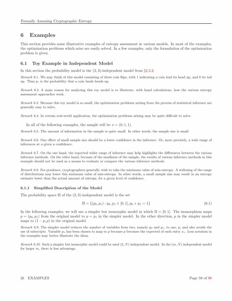
Formally Assessing Cryptographic Entropy
6 Examples
This section provides some illustrative examples of entropy assessment in various models. In most of the examples,the optimization problems which arise are easily solved. In a few examples, only the formulation of the optimizationproblem is given.
6.1 Toy Example in Independent Model
In this section the probability model is the (2, 3)-independent model from §2.3.2.
Remark 6.1. We may think of this model consisting of three coin flips, with 1 indicating a coin lead its head up, and 0 its tailup. Thus p1 is the probability that a coin lands heads up.
Remark 6.2. A main reason for analyzing this toy model is to illustrate, with hand calculations, how the various entropyassessment approaches work.
Remark 6.3. Because this toy model is so small, the optimization problems arising from the process of statistical inference aregenerally easy to solve.
Remark 6.4. In certain real-world application, the optimization problems arising may be quite difficult to solve.
In all of the following examples, the sample will be x = (0, 1, 1).
Remark 6.5. The amount of information in the sample is quite small. In other words, the sample size is small.
Remark 6.6. One effect of small sample size should be a lower confidence in the inference. Or, more precisely, a wide range ofinferences at a given a confidence.
Remark 6.7. On the one hand, the expected wider range of inference may help highlights the differences between the variousinference methods. On the other hand, because of the smallness of the sample, the results of various inference methods in thisexample should not be used as a means to evaluate or compare the various inference methods.
Remark 6.8. For prudence, cryptographers generally wish to take the minimum value of min-entropy. A widening of the rangeof distributions may lower this minimum value of min-entropy. In other words, a small sample size may result in an entropyestimate lower than the actual amount of entropy, for a given level of confidence.
6.1.1 Simplified Description of the Model
The probability space Π of the (2, 3)-independent model is the set
Π = {(p0, p1) : p0, p1 ∈ [0, 1], p0 + p1 = 1} (6.1)
In the following examples, we will use a simpler but isomorphic model in which Π = [0, 1]. The isomorphism mapsp = (p0, p1) from the original model to p = p1 in the simpler model. In the other direction, p in the simpler modelmaps to (1 − p, p) in the original model.
Remark 6.9. The simpler model reduces the number of variables from two, namely p0 and p1, to one, p, and also avoids theuse of subscripts. Variable p1 has been chosen to map to p because p becomes the expected of each entry xi. Less notation inthe examples may better illustrate the ideas.
Remark 6.10. Such a simpler but isomorphic model could be used (2, N) independent model. In the (m,N) independent modelfor larger m, there is less advantage.
§6 EXAMPLES Page 59 of 98

Formally Assessing Cryptographic Entropy 6.1 Toy Example in Independent Model
6.1.2 Maximal Likelihood
For x = (0, 1, 1), the likelihood grading function is
Lx(p) = (1 − p)p2. (6.2)
To help maximize Lx over the probability space [0, 1], we can consider the derivative
Figure 1: Likelihood, Toy Example, with x = (0, 1, 1)
dLx(p)
dp= L′
x(p) = 2p− 3p2 = p(2 − 3p) (6.3)
The critical points of the likelihood function, where L′x = 0, are at p = 0 and p = 2
3 . For the purposes of maximization,we must also consider the boundary of the space Π, which occurs at p = 0, and p = 1. Therefore, we just need toevaluate Lx on each element of the vector (0, 2
3 , 1), which gives (0, 427 , 0). Therefore, the likelihood function attains
its maximal value 427 precisely at p = 2
3 .The set-valued maximal likelihood inference for p is therefore for the set { 2
3}. In a cryptographic application, wemay want infer something about a probability parameter. Since the inferred set is a singleton set, for simplicity, wewill speak of inferred values for the following discussions. The inferred probability distribution is p = 2
3 .The min-entropy H∞(p) of the probability distribution p is as follows. Recall that the inferred probability
distribution is p = 23 . The value of x that maximizes Pp(x) is x = (1, 1, 1), and this gives Pp(x) = 8
27 . Themin-entropy is therefore − log2
(
827
)
which is approximately 1.75 bits of inferred min-entropy for p.
Remark 6.11. The sample used for inference x = (0, 1, 1) and the sample x = (1, 1, 1) used to calculate min-entropy of theprobability distribution inferred from x are not equal. In particular, the sample entropy (information content) of x is higherthan the min-entropy of p.
6.1.3 Threshold Inclusive Typicality
The inclusive typicality with x = (0, 1, 1), works out to be:
g1(x, p) =
3p2 − 2p3 if 0 6 p < 12 ,
1 if p = 12 ,
1 − p3 if 12 < p 6 1,
(6.4)
because: when p > 1/2, the only sample value y with Pp(y) > Pp(x) is y = (1, 1, 1), which has probability Pp(y) = p3;when p = 1/2, the distribution is uniform so the inclusive typicality sums over all samples resulting in 1; when p < 1/2,the set of sample values y with Pp(y) 6 Pp(x), is {(1, 1, 1), (0, 1, 1), (1, 0, 1), (1, 1, 0)}, whose sum of probabilities is3p2(1 − p) + p3 = 3p2 − 2p3. See Figure 2.
§6 EXAMPLES Page 60 of 98
Formally Assessing Cryptographic Entropy 6.1 Toy Example in Independent Model
Figure 2: Inclusive Typicality, Toy Example, with x = (0, 1, 1)
Remark 6.12. The inclusive typicality evaluated at the maximum likelihood estimate for p, from §6.1.2 therefore works out tobe 19
27. The corresponding confidence level is therefore 8
27.
Remark 6.13. Inclusive typicality always takes value 1 at a the uniform distribution p, if the probability model admits auniform distribution. More generally, it will take value 1 at subuniform distributions (see Remark 2.24. If inclusive typicalityis used to formulate a maximally graded inference, then such uniform (and subuniform) distributions will always belong tothe inferred set.
If the inferred set consists of only the uniform distribution, then it maximal inclusive typicality may seem to be a toooptimistic inference method for use in cryptography. In other cases, the inferred set of distributions may contain otherdistributions, and by narrowing the inferred set of entropies by taking its infimum, one may not end up with an overlyoptimistic inference.
For each threshold value t ∈ [0, 1], an inferred set of distributions may be given such that g1/2(x, p) > t, as follows:
ig1>t(x) =
∅ if t = 1
{ 12} if 7
8 6 t < 1[
12 , 3
√1 − t
)
if 12 6 t < 7
8(
q(t), 3√
1 − t)
if 0 6 t < 12
(6.5)
where q(t) is the unique value in [0, 12 ) such that 3q(t)2 − 2q(t)3 = t.
The corresponding inferred sets of min-entropy values are then given by:
H∞ (ig1>t(x)) =
∅ if t = 1
{3} if 78 6 t < 1
(− log2(1 − t), 3] if 0 6 t < 78
(6.6)
Remark 6.14. Recall that H∞(p) depends on the maximum value of Pp(x), which will either by p3 or (1 − p)3.
Cryptographers, in the interest of practicality may wish to narrow the inferred set of min-entropies to a singlevalue, and, moreover, do so by taking the infimum of the set, for the sake of prudence. Instead of thresholds, onemay consider confidence level c = 1 − t. For each confidence level c ∈ [0, 1], the inferred H∞(c) value is given by
H∞(c) =
∞ if c = 0
3 if 0 < c 6 18
− log2(c) if 18 < c 6 1
(6.7)
§6 EXAMPLES Page 61 of 98

Formally Assessing Cryptographic Entropy 6.1 Toy Example in Independent Model
Remark 6.15. In this example, the infima of the inferred sets do not actually belong to the sets.
Remark 6.16. By convention, the infimum of the empty set is (positive) infinity. An inference of infinite amount of entropy ina 3-bit random variable is clearly absurd, but this inference is only made at confidence level 0.
Remark 6.17. The sample entropy (information content) of x = (0, 1, 1), which will be treated later, is certainly higher thanthe inferred min-entropy of p at high confidence levels. Intuitively, at a high confidence levels, close to 1, we must account forthe possibility that p is high, and therefore (1, 1, 1) would have been much more likely than (0, 1, 1).
In this situation, cryptographers may recognize that the sample entropy in (0, 1, 1) is at least log2(3), because we haveassumed the independent model, and the 0 bit could have occurred in any of the three locations. Such sample entropy istherefore useful in cryptography, so we will address its inference in full formality.
6.1.4 Threshold Balanced Typicality
The balanced typicality with x = (0, 1, 1), works out to be:
g 12(x, p) =
32p2 − 1
2p3 if 0 6 p < 12
12 if p = 1
2
1 − 32p2 + 1
2p3 if 12 < p 6 1
(6.8)
Figure 3: Balanced Typicality, Toy Example, with x = (0, 1, 1)
Remark 6.18. The third expression above may be derived as (1 − p)3 + 3p(1 − p)2 + 32p2(1 − p) = 1 − 3
2p2 + 1
2p3.
Remark 6.19. The balanced typicality evaluated at the maximum likelihood estimate for p, from §6.1.2 therefore works out tobe 13
27. The confidence level is therefore 14
27.
Remark 6.20. Balanced typicality is maximized as p approaches 12
from above. Thus typicality and likelihood, in this toyexample, give much difference inferences under maximization. In particular, in this case, typicality may appear too optimistic.It would go too far to conclude from this toy example, however, that maximal typicality is always too optimistic.
For each threshold value t ∈ [0, 1], an inferred set of distributions may be given such that g1/2(x, p) > t, as follows:
ig 12
>t(x) =
∅ if 1116 6 t 6 1
(
12 , q(t)
)
if 12 6 t < 11
16[
12 , q(t)
)
if 316 6 t < 1
2
(r(t), q(t)) if 0 6 t < 316
(6.9)
§6 EXAMPLES Page 62 of 98
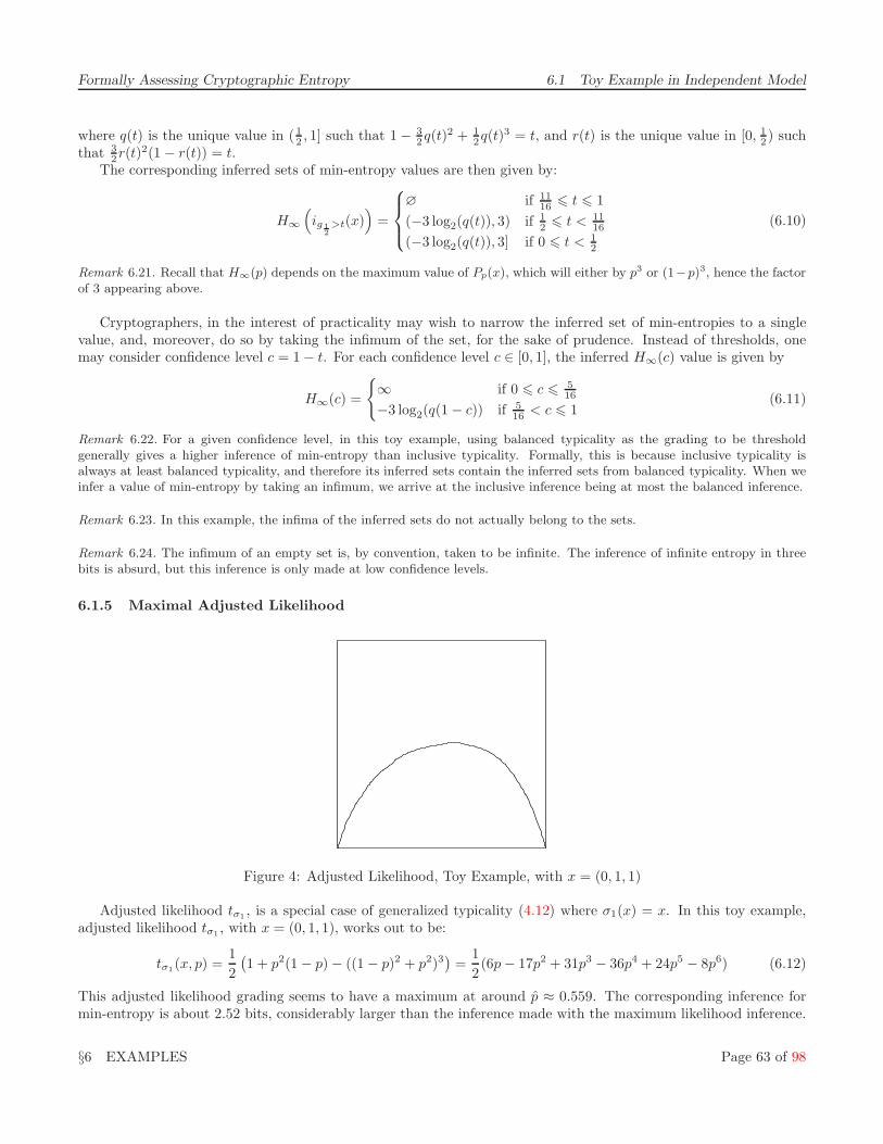
Formally Assessing Cryptographic Entropy 6.1 Toy Example in Independent Model
where q(t) is the unique value in (12 , 1] such that 1 − 3
2q(t)2 + 12q(t)3 = t, and r(t) is the unique value in [0, 1
2 ) suchthat 3
2r(t)2(1 − r(t)) = t.The corresponding inferred sets of min-entropy values are then given by:
H∞(
ig 12
>t(x))
=
∅ if 1116 6 t 6 1
(−3 log2(q(t)), 3) if 12 6 t < 11
16
(−3 log2(q(t)), 3] if 0 6 t < 12
(6.10)
Remark 6.21. Recall that H∞(p) depends on the maximum value of Pp(x), which will either by p3 or (1−p)3, hence the factorof 3 appearing above.
Cryptographers, in the interest of practicality may wish to narrow the inferred set of min-entropies to a singlevalue, and, moreover, do so by taking the infimum of the set, for the sake of prudence. Instead of thresholds, onemay consider confidence level c = 1 − t. For each confidence level c ∈ [0, 1], the inferred H∞(c) value is given by
H∞(c) =
{
∞ if 0 6 c 6 516
−3 log2(q(1 − c)) if 516 < c 6 1
(6.11)
Remark 6.22. For a given confidence level, in this toy example, using balanced typicality as the grading to be thresholdgenerally gives a higher inference of min-entropy than inclusive typicality. Formally, this is because inclusive typicality isalways at least balanced typicality, and therefore its inferred sets contain the inferred sets from balanced typicality. When weinfer a value of min-entropy by taking an infimum, we arrive at the inclusive inference being at most the balanced inference.
Remark 6.23. In this example, the infima of the inferred sets do not actually belong to the sets.
Remark 6.24. The infimum of an empty set is, by convention, taken to be infinite. The inference of infinite entropy in threebits is absurd, but this inference is only made at low confidence levels.
6.1.5 Maximal Adjusted Likelihood
Figure 4: Adjusted Likelihood, Toy Example, with x = (0, 1, 1)
Adjusted likelihood tσ1 , is a special case of generalized typicality (4.12) where σ1(x) = x. In this toy example,adjusted likelihood tσ1 , with x = (0, 1, 1), works out to be:
tσ1(x, p) =1
2
(
1 + p2(1 − p) − ((1 − p)2 + p2)3)
=1
2(6p − 17p2 + 31p3 − 36p4 + 24p5 − 8p6) (6.12)
This adjusted likelihood grading seems to have a maximum at around p ≈ 0.559. The corresponding inference formin-entropy is about 2.52 bits, considerably larger than the inference made with the maximum likelihood inference.
§6 EXAMPLES Page 63 of 98
Formally Assessing Cryptographic Entropy 6.1 Toy Example in Independent Model
6.1.6 Threshold Adjusted Likelihood
The inferred set of min-entropies for a given threshold level t and sample value x = (0, 1, 1) is given by:
H∞(itι>t(x)) =
{
∞ if t > tι(x, p) ≈ 0.504
(−3 log2 q(t), 3] if 0 6 t < tι(x, p)(6.13)
where p is maximal value of adjusted likelihood as described in §6.1.5, and q(t) is now the unique solution in theinterval of [p, 1] of tι(x, q(t)) = t.
At threshold and confidence level c = t = 1/2, the taking the infimum of the inferred min-entropy given anestimate of about 2.11 bits of min-entropy.
6.1.7 Frequency Statistic Induced Inferences
The value of the frequency statistic at sample x = (0, 1, 1) is v = f(x) = (1, 2). The induced probability for v = (1, 2)is
Qp(v) = 3p2(1 − p). (6.14)
6.1.7.1 Maximal Induced Likelihood The induced likelihood is Lv(p) = 3Lx(p) where Lx is the direct like-lihood. So, Lv is maximized at the same value of Lx, which is p = 2
3 . The induced inference for min-entropy istherefore the same as direct inference: about 1.75 bits.
6.1.7.2 Induced Inclusive Typicality The frequency statistic value v = (1, 2) has induced inclusive typicality1 whenever
p ∈[
12 , 3
4
]
. (6.15)
Taking the minimum value of the min-entropy over this range gives an inference of only about 1.24 bits.
Remark 6.25. The directed inference using maximal inclusive typicality was 3 bits of min-entropy, so the use of sample statisticinduced inference has, in this case, reduced the entropy estimate, even though the same inference method was used, namelymaximal inclusive
Remark 6.26. This example shows that the maximal inclusive typicality is not always too optimistic. Indeed, in this case, itseems to be slightly too pessimistic.
More generally the induced inclusive typicality at x = (0, 1, 1) is the function
g1(x, p) =
3p2 − 2p3 if 0 6 p < 11+
√3≈ 0.366
1 − 3p + 6p2 − 3p3 if 11+
√3
6 p < 12
1 if 12 6 p 6 3
4
1 − p3 if 34 < p 6 1
(6.16)
6.1.7.3 Induced Balanced Typicality Induced balanced typicality at x = (0, 1, 1) is the function
g1/2(x, p) =
32p2 − 1
2p3 if 0 6 p < 11+
√3≈ 0.366
112 − 3
√3 ≈ 0.304 if p = 1
1+√
3
1 − 3p + 92p2 − 3
2p3 if 11+
√3
< p < 12
58 if p = 1
2
1 − 32p2 + 3
2p3 if 12 < p < 3
43764 if p = 3
4
1 − 32p2 + 1
2p3 if 34 < p 6 1
(6.17)
§6 EXAMPLES Page 64 of 98

Formally Assessing Cryptographic Entropy 6.1 Toy Example in Independent Model
As p approaches 12 from above, balanced typicality a value of 13
16 ≈ 0.81. The supremum of the balanced typicalitiesis 13
16 , although this value is never attained. One could interpret the maximal frequency-induced balanced typicalityto occur at p = 1
2 + ǫ, for arbitrarily small ǫ > 0. The resulting inference for entropy is about 3− ǫ bits, for arbitrarilysmall ǫ > 0.
In this case, the maximal frequency-induced balanced typicality still seems to produce a inference about min-entropy that is too optimistic.
Remark 6.27. Balanced typicality actually has a local minimum at p = 23, where it takes value 7
9≈ 0.78. As p approaches
34
from below, the typicality approaches 101128
≈ 0.79. At threshold levels, between 79
and 101128
the threshold inferred set is notconnected.
6.1.7.4 Induced Adjusted Likelihood The frequency-induced adjusted likelihood at x = (0, 1, 1) is
tσ1(x, p) = 3p − 21
2p2 +
53
2p3 − 39p4 + 30p5 − 10p6 (6.18)
This function seems to have a maximum at around p ≈ 0.628, so that the maximal frequency-induced adjustedlikelihood estimate for min-entropy is about 2.02 bits.
Remark 6.28. In this case, the effect of inducing on the sample statistic frequency, has reduced the maximum adjusted likelihoodestimate.
6.1.8 Partition Statistic Induced Inferences
The value of the partition statistic at sample x = (0, 1, 1) is θ = φ(x) = (2, 1). The only other possible value of thepartition statistics is θ′ = (3, 0). The induced probability for θ = (2, 1) is
Qp(θ) = 3p(1 − p) (6.19)
6.1.8.1 Maximal Induced Likelihood So the induced likelihood is Lθ(p) = 3p(1 − p) = 3(
14 −
(
p − 12
)2)
.
This form of the likelihood shows to be maximized at p = 12 . The resulting inference for min-entropy is 3 bits.
Remark 6.29. That the partition statistic essentially ignores the values of the entries may in part explain why the maximalinduced likelihood distribution does not favor 1 or 0.
6.1.8.2 Maximal Induced Inclusive Typicality Because the partition statistic in the (2, 3) independent modelcan only takes two values, statistic value θ = (2, 1) has induced inclusive typicality 1 when 3p(1 − p) > 1
2 , whichholds whenever
p ∈[
12 −
√
112 , 1
2 +√
112
]
. (6.20)
Taking the minimum value of the min-entropy over this range gives an inference of only about 1.02 bits.
6.1.9 Bayesian Inference
Bayesian inference requires an a priori distribution on the probability space Π. For this example, let us assume auniform distribution on Π = [0, 1]. For x = (0, 1, 1), recall that the standard likelihood grading was Lx(p) = p2(1−p),so the Bayesian grading works out to be:
Bx(p) =p2(1 − p)
∫ 1
0 p2(1 − p)dp= 12p2(1 − p). (6.21)
Because this grading is just a constant scaling of the likelihood grading, it gives the same maximally graded inference.It is unclear how to use grading for thresholding.
§6 EXAMPLES Page 65 of 98
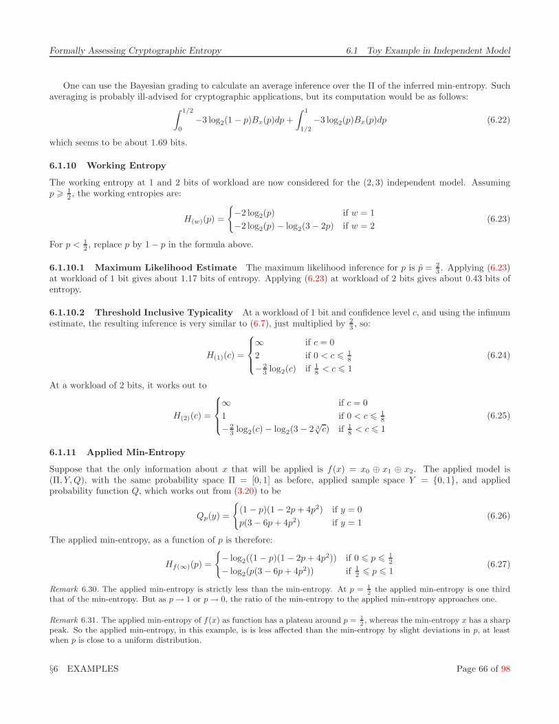
Formally Assessing Cryptographic Entropy 6.1 Toy Example in Independent Model
One can use the Bayesian grading to calculate an average inference over the Π of the inferred min-entropy. Suchaveraging is probably ill-advised for cryptographic applications, but its computation would be as follows:
∫ 1/2
0
−3 log2(1 − p)Bx(p)dp +
∫ 1
1/2
−3 log2(p)Bx(p)dp (6.22)
which seems to be about 1.69 bits.
6.1.10 Working Entropy
The working entropy at 1 and 2 bits of workload are now considered for the (2, 3) independent model. Assumingp > 1
2 , the working entropies are:
H(w)(p) =
{
−2 log2(p) if w = 1
−2 log2(p) − log2(3 − 2p) if w = 2(6.23)
For p < 12 , replace p by 1 − p in the formula above.
6.1.10.1 Maximum Likelihood Estimate The maximum likelihood inference for p is p = 23 . Applying (6.23)
at workload of 1 bit gives about 1.17 bits of entropy. Applying (6.23) at workload of 2 bits gives about 0.43 bits ofentropy.
6.1.10.2 Threshold Inclusive Typicality At a workload of 1 bit and confidence level c, and using the infimumestimate, the resulting inference is very similar to (6.7), just multiplied by 2
3 , so:
H(1)(c) =
∞ if c = 0
2 if 0 < c 6 18
− 23 log2(c) if 1
8 < c 6 1
(6.24)
At a workload of 2 bits, it works out to
H(2)(c) =
∞ if c = 0
1 if 0 < c 6 18
− 23 log2(c) − log2(3 − 2 3
√c) if 1
8 < c 6 1
(6.25)
6.1.11 Applied Min-Entropy
Suppose that the only information about x that will be applied is f(x) = x0 ⊕ x1 ⊕ x2. The applied model is(Π, Y, Q), with the same probability space Π = [0, 1] as before, applied sample space Y = {0, 1}, and appliedprobability function Q, which works out from (3.20) to be
Qp(y) =
{
(1 − p)(1 − 2p + 4p2) if y = 0
p(3 − 6p + 4p2) if y = 1(6.26)
The applied min-entropy, as a function of p is therefore:
Hf(∞)(p) =
{
− log2((1 − p)(1 − 2p + 4p2)) if 0 6 p 6 12
− log2(p(3 − 6p + 4p2)) if 12 6 p 6 1
(6.27)
Remark 6.30. The applied min-entropy is strictly less than the min-entropy. At p = 12
the applied min-entropy is one thirdthat of the min-entropy. But as p → 1 or p → 0, the ratio of the min-entropy to the applied min-entropy approaches one.
Remark 6.31. The applied min-entropy of f(x) as function has a plateau around p = 12, whereas the min-entropy x has a sharp
peak. So the applied min-entropy, in this example, is is less affected than the min-entropy by slight deviations in p, at leastwhen p is close to a uniform distribution.
§6 EXAMPLES Page 66 of 98

Formally Assessing Cryptographic Entropy 6.1 Toy Example in Independent Model
6.1.11.1 Maximal Likelihood At the maximal likelihood inference p = 23 the applied min-entropy is about
− log2(1427 ) ≈ 0.948 bits.
6.1.11.2 Inclusive Typicality Taking the infimum of threshold inclusive typicality inference, gives the following:
Hf(∞)(c) =
∞ if c = 0
1 if 0 < c 6 18
− log2(33√
c − 63√
c2 + 4c) if 18 < c 6 1
(6.28)
at a confidence of c.
6.1.12 Contingent Min-Entropy
Suppose that the adversary can learn the function f(x) where f is defined as:
f(x) =
{
0 if x ∈ {(0, 0, 0), (1, 1, 1)},1 otherwise.
(6.29)
Remark 6.32. One reason that an adversary might learn such a function f(x) is that the amount of inferred entropy maydepend strongly on the function f(x), and thus the actions that would be taken by cryptographic implementation in an effortto gather enough entropy would need to differ, thereby creating a higher chance of a side channel.
Remark 6.33. Another possible reason that an adversary might learn such a function is that f(x) is the exclusive-or of thebits in the representation of x0 + x1 + x2.
For given p ∈ Π, the general formula (3.22) for contingent min-entropy works out to be:
H∞|f (p) =
{
−2 log2(1 − p) if 0 6 p 6 12
−2 log2 p if 12 6 p 6 1
(6.30)
Remark 6.34. For example, when p = 12, the contingent entropy is 2 bits. Intuitively, this is because an adversary has a
strategy to guess x with probability 14.
One such strategy is to guess x = (0, 0, 0) when f(x) = 0 and to guess x = (0, 0, 1) when f(x) = 1.The first case occurs 1
4of the time, and the adversary guess is right 1
2of that time, making for a correct guess 1
8of the
time. The second case occurs 34
of the time and the adversary’s guess is right 16
of that time, making for a correct guess 18
oftime. These correctly-guessed times are disjoint and total to 1
4.
The contingent min-entropy in this example works out to always be exactly 23 of the min-entropy. Therefore, all
the inferences for min-entropy will scale exactly 23 for inferences of contingent min-entropy.
6.1.13 Filtered Min-Entropy
Suppose that an implementation of a source assumed to be in (2, 3) independent model will reject a sample outputof (0, 0, 0) or (1, 1, 1), perhaps on the ground that these sample could have arisen from a deterministic distributionin the independent model.
Therefore, the adversary wishing to guess x can exclude these values. For cryptographic purposes, one mustconsider the filtered entropy of x based on the knowledge that the adversary would possess. In other words, theadversary has knowledge that x ∈ Y ( X where Y = {(0, 0, 1), (0, 1, 0), (1, 0, 0), (0, 1, 1), (1, 0, 1), (1, 1, 0)}. Applying(3.26), maximizing, and taking the negative logarithm to the base two, yields a filtered min-entropy value of:
log2(3) − log2(max(p, 1 − p)) (6.31)
The inferred set of distribution for p does not depend on the parameter, so to infer the filtered entropy, it will sufficeto apply the filtered entropy to the inferred sets, and take infima.
§6 EXAMPLES Page 67 of 98

Formally Assessing Cryptographic Entropy 6.1 Toy Example in Independent Model
6.1.13.1 Maximum Likelihood Estimate The maximum likelihood inference gives p = 23 . Applying (6.31)
gives an inferred filtered entropy of 2 log2(3) − 1 ≈ 2.17 bits of filtered entropy.
6.1.13.2 Threshold Inclusive Typicality At confidence level c, the filtered entropy, works out to be (byadapting (6.7)),
Ic(x) =
∞ if c = 0
log2(3) + 1 if 0 < c 6 18
log2(3) − 13 log2(c) if 1
8 < c 6 1
(6.32)
Remark 6.35. As confidence levels c approaches 1, the threshold inclusive typicality inferred min-entropy approaches 0, whilethe threshold inclusive inferred filtered entropy approaches log2 3 ≈ 1.58.
The reason that inferred min-entropy is much lower is that it allows for the possibility of x = (1, 1, 1), which could occurwith probability nearly 1 when the confidence level approaches 1. By contrast, the filtered entropy, as defined above, does notallow x = (1, 1, 1), because (1, 1, 1) is filtered.
Remark 6.36. In a cryptographic application, this example is a little artificial. In the case of prospective assessment, as c → 1,the inferred min-entropy approaches 0, because p → 1. A source is likely to result in (1, 1, 1) and therefore by rejected.
So, as noted before, the possibility of rejection is not reflected in the definition of filtered entropy. If the source can befreely sampled until the result is not rejected, then indeed, the higher inferred contingent entropy properly reflects reality.
But in this report, it is generally presumed that the source is expensive to sample. So, a low inferred min-entropy doesreally reflect something about the rate at which entropy can be drawn from the source.
6.1.14 Sample Entropy
In this section, inferences about the sample-dependent parameter sample entropy (§3.3.1) are made.
Remark 6.37. Recall that sample entropy is mainly useful retrospective inference.
Remark 6.38. Most inference methods given sample x = (0, 1, 1) in the (2, 3) independent model infer a set of distributionswhose min-entropy infimum distribution has p > 1
2, roughly because 1 appears more often than 0 in the sample x. For such
a distribution with p > 12, the sample value (1, 1, 1) is at least as likely the given sample. Indeed, when p > 1
2, the sample
(1, 1, 1) is more likely, and is the sample which gives rise to the min-entropy of the distribution p.In these cases, x = (0, 1, 1) has sample entropy at least as high as the min-entropy of p.
Remark 6.39. One usually applies retrospective inference, when one does not wish to waste entropy, so a higher value of sampleentropy is not to be discarded.
The inferred set of probability distribution is the same as for min-entropy. The remaining task is to apply thesample entropy parameter, and then take the infimum.
6.1.14.1 Maximal Likelihood Taking the maximum likelihood inference gives p = 23 for the solely inferred
distribution. The inferred sample entry is I(p, x) = − log2(p2(1 − p)) = 3 log2(3) − 2 ≈ 2.75.
Remark 6.40. By comparison, the inferred sample entropy 2.75 is exactly 1 bit greater than the inferred min-entropy 1.75,under the same inference method (maximal likelihood estimation).
6.1.14.2 Threshold Inclusive Typicality Each threshold level t determines, under threshold inclusive typical-ity, a set of inferred distributions ig1>t(x), which were calculated in (6.5). Applying the parameter sample entropy
§6 EXAMPLES Page 68 of 98
Formally Assessing Cryptographic Entropy 6.1 Toy Example in Independent Model
p 7→ I(p, x) to each of these subsets of Π, seems to gives
I(ig1>t(x), x) =
∅ if t = 1
{3} if 78 6 t < 1
(
− log2
(
t − 1 + (1 − t)2/3)
, 3]
if 1927 6 t < 7
8
[3 log2(3) − 2, 3] if 12 6 t < 19
27
[3 log2(3) − 2,− log2 (q(t))] if 0 6 t < 12
(6.33)
where q(t) is the function taking value in interval [0, 12 ] such that 3q(t)2 − 2q(t)3 = t.
Remark 6.41. At thresholds below 12, the inferred interval of sample entropies contains values larger than 3, which is an
instance of Remark 3.50.
For confidence level c = 1 − t the infimum of the inferred sample entropies is:
Ic(x) =
3 log2(3) − 2 if c > 827
− log2(−c + c2/3) if 18 < c 6 8
27
3 if 0 < c 6 18
∞ if c = 0
(6.34)
6.1.15 Eventuated Min-Entropy
Suppose that the probability model is the (2, 5) independent model but that, at the time of making inference aboutp, the first three bits of x have been observed to be (0, 1, 1). So, in other words, the event E that has occurred isthat (x0, x1, x2) = (0, 1, 1).
The first three bits of the x adhere to the (2, 3) independent model, so the inferences to be made about p arethose that would be made in (2, 3) independent. In particular, the inferences about p of the subsections above apply.In this section, inferences will be made about the sample-dependent parameter eventuated min-entropy (§3.3.2).
The eventuated min-entropy is
H∞‖E(p, x) = − log2(1 − p)p2 max(p, 1 − p)2 (6.35)
6.1.15.1 Maximal Likelihood The maximum likelihood inference for p was p = 23 (actually a singleton set),
from §6.1.2.The inferred eventuated min-entropy under maximum likelihood inference is therefore 5 log2(3) − 4 ≈ 3.92 bits.
6.1.15.2 Threshold Inclusive Typicality Applying the infimum value of the eventuated min-entropy param-eter H∞‖E from (6.35) to each of the threshold inclusive typicality inferred sets of distributions from (6.5), andexpressing the results as a function of the confidence level c = 1 − t, gives
H∞‖E:g1>(1−c)(x) =
∞ if c = 0
5 if 0 < c 6 18
− 43 log2 c − log2(1 − 3
√c) if 1
8 < c 6 64125
5 log2(5) − 8 ≈ 3.61 if 64125 6 c 6 1
(6.36)
Remark 6.42. The distribution p = 45
actually minimizes the eventuated min-entropy. Consequently at high enough confidencelevels, specifically, as shown above, the infimum of the inferred eventuated min-entropies is realized at p = 4
5.
Recall that the adversary is presumed to know p. When p > 12, the generally optimum single guess at x for adversary is
to guess x = (1, 1, 1, 1, 1). Because the event E has occurred this optimum strategy will fail, because x0 = 0 in the event Eand x0 in the optimal guess..
Nevertheless, eventuated min-entropy attempts to account for all possible strategies, including a strategy to guess x =(0, 1, 1, 1, 1). What eventuated min-entropy measures is the general success rate of such a strategy as if the event E had notoccurred.
§6 EXAMPLES Page 69 of 98
Formally Assessing Cryptographic Entropy 6.1 Toy Example in Independent Model
6.1.16 Applied Eventuated Min-Entropy
Suppose that the probability model is the (2, 5) independent model but that, at the time of making inference aboutp, the first three bits of x have been observed to be (0, 1, 1). So, in other words, the event E that has occurred is that(x0, x1, x2) = (0, 1, 1). Explicitly, E = {(0, 1, 1, 0, 0), (0, 1, 1, 0, 1), (0, 1, 1, 1, 0), (0, 1, 1, 1, 1)}. Furthermore, supposethat only the middle three bits f(x) = (x1, x2, x3) are to be used.
The first three bits of the x adhere to the (2, 3) independent model, so the inferences to be made about p are thosethat would be made in (2, 3) independent. In particular, the inferences about p of the subsections above apply. Inthis section, inferences will be made about the sample-dependent parameter applied eventuated min-entropy (§3.3.3).
The applied eventuated min-entropy is
Hf(∞)‖E(p, x) = − log2 p2 max(p, 1 − p) (6.37)
6.1.16.1 Maximal Likelihood The maximum likelihood inference for p was p = 23 (actually a singleton set),
from §6.1.2. The inferred eventuate min-entropy under maximum likelihood inference is therefore 3 log2(3)−3 ≈ 1.75bits.
6.1.16.2 Threshold Inclusive Typicality Applying the infimum value of the eventuated min-entropy param-eter Hf(∞)‖E from (6.37) to each of the threshold inclusive typicality inferred sets of distributions from (6.5), andexpressing the results as a function of the confidence level c = 1 − t, gives the same inferred entropy as the inferredmin-entropy from (6.7).
Remark 6.43. For high confidence c, the inferred applied eventuated min-entropy approaches zero in this example, whereaseventuated min-entropy in the previous example did not approach zero. The main difference accounting for this is that herethe adversary’s ideal strategy (not hinging on event E), knowing p > 1
2is to guess f(x) = (1, 1, 1), whereas in the previous
example, for p > 12
(not hinging on event E), the adversary’s ideal strategy was to guess (1, 1, 1, 1, 1).
6.1.17 Contingent Eventuated Min-Entropy
Suppose that the model is the (2, 5) independent model. Suppose that, at the time of making an inference, the eventE concerning the sample x that (x0, x1, x2) = (0, 1, 1) is observed. Suppose that the adversary will learn the valueof g(x) where g is the function g : X → {0, 1, 2, 3, 4, 5} : x 7→ x0 + x1 + x2 + x3 + x4. The contingent eventuatedmin-entropy from §3.3.4 may be inferred as follows.
A function f supplementary to g that may minimize the applied eventuated min-entropy Hf(∞)‖E)(p, x) is afunction f : X → {0, 1, 2, . . . , 9} such that
f :
(0, 1, 1, 0, 0) 7→ 0
(0, 1, 1, 0, 1) 7→ 0
(0, 1, 1, 1, 0) 7→ 1
(0, 1, 1, 1, 1) 7→ 0
(6.38)
and such that, for each j ∈ {0, 1, 2, 3, 4, 5}, the function f maps g−1(j) injectively into the set {0, 1, . . . ,(
5j
)
− 1}. Ifthis function f does indeed minimize the applied min-entropy, then contingent min-entropy is given by
H∞|g‖E(p, x) = − log2 p2(1 − p)((1 − p)2 + (1 − p)p + p2) (6.39)
Contingent eventuated min-entropy seems to have a minimum at
p =8 +
3√
107 + 15√
129 +3√
107 − 15√
129
15≈ 0.702 (6.40)
§6 EXAMPLES Page 70 of 98

Formally Assessing Cryptographic Entropy 6.2 Polling Inference
6.2 Polling Inference
Examples of inference in the (2, N) independent model, with N ≫ 2 are considered in this section.As in §6.1, we use the simplified description of the model, in which Π = [0, 1], with distribution p mapping to
distribution (1 − p, p) in the standard description of the model.Whereas §6.1, and §6.3 could be considered as low sample size inferences in the independent model, the example
in this section could be considered as a large sample size. Intuition suggests the inferences should have higherconfidence levels, and that the resulting inference depend less on the inference method.
This example could arise in various ways. Coins could have been flipped, either one coin N times, or N coinsonce, or something in between. This type of inference also arises in non-cryptographic applications such as in polling:say N people are queried on a yes or no.
It is again emphasized that the independent model is being assumed in this section, not assessed. Again, it isassumed that the N bits are independent and identically distributed. It is under these assumptions that inferenceswill be made.
Each example will address a distinct inference method. A first part of each example may treat the general caseof any N and any sample x. For the sake concreteness, a second part of each example may treat a specific choice ofN and x. For consistency of comparison, each example will use the same specific N and x. For ease of computation,the fairly small choice N = 32 will be used. For x, we will use:
x = (1, 0, 0, 1, 1, 0, 0, 1, 0, 1, 1, 1, 0, 1, 1, 1, 0, 1, 1, 1, 0, 0, 1, 1, 1, 0, 1, 0, 1, 0, 1, 1) (6.41)
This value x has 20 entries of value 1, and 12 of value 0. In the independent model, the order of the entries doesnot matter, so the 20 ones could be have appeared first, following by the zeroes, without affecting the inferences. Ofcourse, if the probability model was a Markov, then the order of the bits is crucially important.
Remark 6.44. The value of x above is derived from the binary expansion of√
23. Taking into account the specialized mannerin which this x was actually selected produces a model much different than the independent model, which would likely yieldmuch lower entropy estimates.
6.2.1 Maximum Likelihood
Recall that likelihood function is Lx(p) = Pp(x) = (1 − p)f(x)0pf(x)1 , where f(x) is the frequency vector §5.4.2 of x.Just as the probability model was given a simplified description, we simplify the frequency vector to a scalar f(x)counting the number of ones in x. (So, the former frequency vector is now (N − f(x), f(x))). In this notation,
Lx(p) = (1 − p)N−fpf (6.42)
To maximize Lx, calculate its derivative as L′x(p) = −(N − f)(1− p)N−f−1pf + f(1− p)N−fpf−1 = (f(1− p)− (N −
f)p))(1 − p)N−f−1pf−1 = (). For 0 < f < N , the solutions to L′x(p) = 0 are p = 0 and p = f
N and p = 1. (At f = 0and f = N , the solutions are p = 1 and p = 0 respectively.) Because Lx is differentiable, any local maximum p mustoccur at a critical point with Lx(p) = 0, or at boundary of Π = [0, 1]. It is straightforward to confirm, p = f
N is theglobal maximum in [0, 1] for all 0 6 f 6 N . (
Remark 6.45. For the f ∈ {0, N} the global maximum occurs at a boundary point where L′x(p) 6= 0. Otherwise the global
maximum occurs at a local minimum interior to the domain [0, 1].
With the specific choices of x from (6.41), we get an inferred distribution of p = 2023 = 5
8 .The inferred min-entropy is H∞(p) = − log2 Pp(x) = − log2 p32 ≈ 21.7 bits. This is due the the fact p > 1
2 makesthe sample x = (132) the most likely sample value.
§6 EXAMPLES Page 71 of 98

Formally Assessing Cryptographic Entropy 6.2 Polling Inference
6.2.2 Inclusive Typicality
Using the notation f(x) from §6.2.1, the inclusive typicality is:
g1(x, p) =∑
y:Pp(y)6Pp(y)
Pp(y)
=∑
y:(1−p)N−f(y)pf(y)6(1−p)N−f(x)pf(x)
(1 − p)N−f(y)pf(y)
=
∑Ne=f(x)
(
Ne
)
(1 − p)N−epe if 0 6 p < 12
1 if p = 12
∑f(x)e=0
(
Ne
)
(1 − p)N−epe if 12 < p 6 1
(6.43)
The inclusive typicality at the maximum likelihood estimate p is about 0.566. The inclusive typicality as p approaches12 from above (but not at 1
2 ) is about 0.945.If we want to have confidence level of 0.999, which corresponds to a threshold of 0.001, then the largest value of
p meeting this threshold is p ≈ 0.857. The corresponding infimum inference for the min-entropy of p seems to 7.12bits of entropy.
Remark 6.46. Generally, as N approaches infinity, if f(x) > N2
, then, at all but the most lowest and highest threshold levels,
the inferred set of distributions takes the form of an interval [a, b] where a = 12
and b ≈ f(x)N
. Indeed, in the interval [a, b], thetypicality is nearly one, and elsewhere is is nearly zero.
The upper end of the interval corresponds to the maximum likelihood estimate.The lower bound of the interval reflects the fact that for distributions p ' 1
2, The function Pp of the sample x is sufficiently
flat in the sense that with probability near to 1, it holds that Pp(y) 6 Pp(x).
Remark 6.47. A more precise description of the approximate shape of the inclusive typicality for large N is given by the Gausserror function.
Remark 6.48. From the perspective of general inference, the inference from inclusive typicality may seem too weak, in that italways infers some distributions close to 1
2, whereas one might expect that inference should strongly value distributions near
to f(x)N
. (Sample statistic induced inference may resolve this.)From the perspective of cryptography, the arguable weakness of the inference makes no difference in this case, because by
taking the infimum of the entropies in the interval, we find the infimum is unaffected by the inclusion of distributions near to12.
6.2.3 Balanced Typicality
As N gets larger, the difference between inclusive and balanced typicality becomes negligible compared to the totaltypicality.
6.2.4 Adjusted Likelihood
The adjusted likelihood seems to take a maximum value at p ≈ 0.5516. The inferred min-entropy is then about 27.5bits.
6.2.5 Frequency Statistic Induced Inference
The induced likelihood of frequency is proportional of the standard likelihood in the sense that Lf(x)(p) =(
Nf
)
Lx(p),
so taking the induced inference under maximal likelihood is the same, namely p = f(x)N .
The frequency induced inclusive typicality takes the form
g1(f, p) =
a(f,p)∑
e=0
+
N∑
e=b(f,p)
(
N
e
)
pe(1 − p)N−e (6.44)
§6 EXAMPLES Page 72 of 98

Formally Assessing Cryptographic Entropy 6.3 Low Sample Sizes in the Independent Model
where a(f, p) and b(f, p) are integers determined by f and p, because the likelihood function is unimodal, increasingfor f 6 pN and decreasing for f > pN . So, a(f, p) = f if f 6 pN and b(f, p) = f if f > pN .
For large N , the probability function takes the shape of a normal curve, due to the Central Limit Theorem. Thissuggests the approximations a(f, p) ≈ pn − |pn − f | and b(f, p) ≈ pn + |pn − f |.
For the specific N = 32 and sample x from (6.41), which has f(x) = 20, the function p 7→ g1(f, p) from (6.44)was estimated using floating point arithmetic at value p = m
8192 for integers m with 0 6 m 6 8192, and plotted asshown in Figure 5.
Remark 6.49. The non-smooth, stepped appearance of the graph seems to be the actually correct effect of the shifting summa-tion term limits, and is not merely some round effect. As N gets, this curve should probably approach a smoother curve. Theshape of Figure 5 might suggest that as N goes to infinity, the curve would approach in shape a normal curve, but actuallyit should approach in shape the sum of Gauss error function and an reflected Gauss error function. The curve will be smoothexcept for a sharp peak at the maximum.
Figure 5: Frequency-Induced Inclusive Typicality Plot in the (2, 32) independent model
Remark 6.50. By just casually glancing at Figure 5, at a confidence level of 0.9, the inferred set of distributions seems to beabout [0.47,0.75]. Applying the min-entropy parameter gives an inferred set of about [13.28,32]. Taking the infimum of themin-entropies, gives 13.83 bits of entropy at a 90% confidence level.
Remark 6.51. Maximal inclusive typicality should in theory be obtained whenever p gives a peak in the likelihood at frequencyvalue f = 20, which should occur when p ∈ [ 19
32, 20
32]. Figure 5 is only slightly off from this.
6.3 Low Sample Sizes in the Independent Model
The hypothetical example from §1.1.2.8 is now addressed under the formal approaches of this report. Recall thatthe independent probability model was assumed. Specifically, the (m, N) independent with m = 232.
§6 EXAMPLES Page 73 of 98
Formally Assessing Cryptographic Entropy 6.3 Low Sample Sizes in the Independent Model
Remark 6.52. Some heuristic justification for the independent model. Muons are elementary particles similar to electrons butmuch more massive. Because of their large mass, creation of muons requires amounts of localized energy so large that theytypically do not arise to nuclear reactions. Thus creation of muons on earth requires accelerators.
Muons passing through the atmosphere arise from the cosmic rays, primarily intergalactic protons that have been accel-erated by galactic magnetic fields over very long distances to very high speeds. These protons strike atoms in the atmosphereand create muons. The muons then continue in the nearly the same direction as the original proton, ionizing atoms along theway, until the muons decay into a high-energy electron and neutrinos. Because of the mass, charge, and high speed of cosmicray muons, they are highly penetrating and can be used to form images of the moon kilometers underground.
Given the above, it seems not unreasonable that each muons passing through a detector may be independent. Especiallysuggestive of this assumption would the intergalactic source: since perhaps muons from different directions would have sourcesvery far apart within the universe, and ought to have independent speeds.
Of course, hypothesis testing can be applied to this assumption. Possible reasonable causes for lack of independence mightbe bursts or regularity of muons from a certain directions of the universe.
In our hypothetical example, a third party laboratory is assessing the source, collecting N = 1024 muon measures,so the model from the lab’s perspective is the (m, N) = (232, 210) independent model. Because N ≪ m, the samplesize may be deemed as low.
Recall the supposition that the laboratory observes 1023 distinct values among the 1024 muon speed measure-ments. In other words, one value repeats and all other values are distinct. Because the independent model is assumed,the actual values and the order in which they occurred are irrelevant for inferring entropy. The independent modelimplies that the assessed entropy is a function of sorted frequencies. So, without loss of generality, it can be assumedthat x = (x0, x1, . . . , xN−1) = (0, 0, 1, . . . , N − 2).
Because the independent model is assumed, each muon measurement contributes equally to the entropy. The labcan divide its overall assessment by N to determine the entropy per component. This will determine the amount ofentropy per muon measurement.
The lab’s observations will not include the sample values used in cryptographic applications. So the entropyassessment will be prospective. In the field where the source is deployed, if the assessed min-entropy per componentis h bits, and the goal it is to obtain to k bits of min-entropy, then a value of N = ⌈k/h⌉ can be used.
6.3.1 Maximal Likelihood Estimate
It is verified below that the maximal likelihood estimate inference for the probability distribution p is to take therelative frequencies of from the sample x. More precisely, the maximal likelihood inference for the distribution is theset {p}, where
pi =
2N if i = 01N if 1 6 i 6 N − 2
0 if N − 1 6 i 6 m − 1
(6.45)
The set-value inference for the min-entropy is then {H∞(p)}. Narrowing the set-valued inference to a point-valuedinference, by taking the minimum, and evaluating the result numerically gives 9216 bits of min-entropy, which is 9bits of min-entropy per component of x.
Remark 6.53. This estimate is considerably lower than the heuristic argument for about 20 bits in the introduction. On onehand, a lower estimate is more prudent, causing the implementer to seek out more entropy. On the other hand, a low entropyestimate is expensive, because more entropy has to be gathered which can be costly.
The verification mentioned above for given maximum likelihood estimate for independent model is as follows.Apply (A.10) to the objective f
f(p) = −Lx(p) = −p20p1p2 . . . pN−1 (6.46)
The gradient of the f is given by
∇f(p) = (2Λ/p0, Λ/p1, . . . , Λ/pN−2, 0, . . . , 0), (6.47)
§6 EXAMPLES Page 74 of 98

Formally Assessing Cryptographic Entropy 6.3 Low Sample Sizes in the Independent Model
where Λ = −Lx(p), provided none of p0, . . . , pN−2 are zero. If any of p0, p1, . . . , pN−2 are zero, then the likelihood iszero, and it is easy to find p such that the likelihood is positive. Therefore, we can assume that none of p0, . . . , pN−2
are zero.The right hand side of (A.10) can be seen to be simply NΛ. Therefore the m inequalities of (A.10) becomes,
upon multiplication of appropriate denominators and division by NΛ < 0 become
2/N 6 p0 (6.48)
1/N 6 p1, . . . , pN−2 (6.49)
0 > pN−1, . . . , pm−1 (6.50)
which, with the usual defining conditions on the probability distribution p, implies the result claimed above.
Remark 6.54. The inclusive typicality of the the sole distribution p in the maximum likelihood inferred set has value
g1(x, p) =
„
1 − 2
N
«N „
5 +10
N − 2+
4
(N − 2)2
«
≈ 0.68 (6.51)
which is less than 1, because other sample values have higher probability than x, in particular, any sample y in which thecomponent 0 appears more than twice, and all other components are at most N − 2. In particular, the most likely sample is(0, 0, . . . , 0), and this is the sample value, that an adversary knowing p = p, should guess. This sample is 2N−2 times moreprobable than the obtained sample x, under the inferred distribution p.
Remark 6.55. The balanced typicality of the the sole distribution p in the maximum likelihood inferred set has value
g1(x, p) =
„
1 − 2
N
«N „
4 +4
N − 2+
2
(N − 2)2
«
≈ 0.54 (6.52)
which is more than 1/2, indicating that the p has higher balanced typicality than any subuniform distribution consistent withx.
6.3.2 Maximal Inclusive Typicality
Inclusive typicality always takes a maximal value of 1. For the given sample x, the inclusive typicality is 1 providedPp(x) > Pp(y) for all y ∈ X . We claim that this will be true whenever:
p0 = p1 = · · · = pN−2 > pN−1, . . . , pm, (6.53)
because Pp(x) = p20p1 . . . pN−2. To prove this claim, suppose otherwise. This supposition implies pi < pj for some
i, j with i 6 N − 2. Replace a pi by a pj to get a Pp(y) > Pp(x). More precisely, let yi+1 = j and let yk = xk fork 6= i + 1.
This set of probability distributions given by (6.53) is more extensive than that given by a maximum likelihoodestimate. For example, it includes the (fully) uniform distribution. The directly inferred set of min-entropies iscorrespondingly extensive. For example, in includes the inference of log2(N) bits.
Nevertheless, taking the minimum inferred min-entropy corresponds to the probability distribution in whichpi = 1/(N − 1) for i ∈ [0, N − 2] and otherwise pi = 0. For the choice of N = 210, we get an inferred min-entropylog2(2
10 − 1) ≈ 9.9986 bits of entropy per component of x.
Remark 6.56. This gives an estimate of almost one more bit of entropy than we obtained from maximal likelihood estimate.
Remark 6.57. This estimate is still considerably lower than the heuristic argument for about 20 bits in the introduction.
Remark 6.58. The probability distribution at which the minimum inferred entropy is attained is a subuniform distribution,specifically an (N − 1, m)-subuniform distribution.
§6 EXAMPLES Page 75 of 98

Formally Assessing Cryptographic Entropy 6.3 Low Sample Sizes in the Independent Model
6.3.3 Maximal Balanced Typicality
Consider distributions p with inclusive typicality of 1, that also approach the uniform distribution X . The balancedtypicality of these distributions approaches:
1 − 1
2
(
N − 1
m
)N
(6.54)
or about 1 − 222000, which is very close to 1. If these distributions have higher balanced typicality than any others,then the maximal balanced typicality is a limit, with no actual distribution hitting the maximum. Nevertheless, thelimit of the distributions exists and is the uniform distribution, which gives an estimate of 32 bits of min-entropyper component.
Remark 6.59. At this point, the assessments seem too pessimistic or too optimistic compared to the intuition from theintroduction. Indeed, the introduction informally makes use of a sample statistic.
6.3.4 Frequency Statistic Induced Inference
The function s : X → Y given by the frequency statistic defined in §5.4.2 induces probability model (Π, Y, Q) suchthat
Qp(y) = M(y)Pp(x) (6.55)
where x ∈ X is such that s(x) = y and M(y) is an integer multiplier counting that the number of x such thats(x) = y. This holds from (5.1) because that statistic s has the property that for all x, x′ ∈ X and p ∈ Π ifs(x) = s(x′) then Pp(x) = Pp(x
′).With our specific sample gathered of x = (0, 0, 1, . . . , N −2), we have y = s(x) = (2, 1, . . . , 1, 0, . . . , 0) where there
are N − 2 entries with value 1 and m − N + 1 entries with value 0.The general formula for the integer multiple M(y) is given by M(y) = N !
y0!y1!...ym! . The general formula for theprobability of y is therefore:
N !m∏
i=0
pyi
i
yi!(6.56)
With our specific sample example gathered y, the value of the multiplier is thus N !/2 and the probability is12N !p2
0p1 . . . pN−2.
6.3.4.1 Induced Inclusive Typicality Consider the distribution p maximal likelihood inference from (6.45).The frequency-induced inclusive typicality of y = s(x) at distribution p is one. Therefore the maximal inducedinclusive typicality consists of all distributions p reaching induced typicality of one. Taking the infimum of min-entropies over this set will be at most H∞(p), which as above, is 9 bits per component.
Similarly, any threshold graded inference with the frequency-induced inclusive typicality will give, once one takesan infimum of min-entropies, will give at most 9 bits of min-entropy per component of the sample.
6.3.4.2 Induced Balanced Typicality Let u be an integer with N 6 u 6 m. Let S be a (u−2)-element subsetof {1, . . . , m − 2}, such that {1, . . . , N − 2} ⊆ S. Let pS be a distribution defined by
pSi =
2/u if i = 0
1/u if i ∈ S
0 if i 6∈ S
(6.57)
The frequency-induced inclusive typicality of x at pS is one, and as such, the distributions pS would seem to goodcandidates for maximizing balanced typicality. The frequency-induced balanced typicality of x at pS seems to be:
1 − 1
4
(
m − N + 1
u − N
)
N !
uN(6.58)
§6 EXAMPLES Page 76 of 98
Formally Assessing Cryptographic Entropy 6.4 Toy Examples in the Markov Model
This seems to be maximized when u = N . When u = N , the distribution pS is the same as distribution in themaximal likelihood inference.
This suggests that threshold frequency-induced balanced typicality inferences would be similar to thresholdfrequency-induced inclusive typicality inferences.
6.3.4.3 Induced Threshold Adjusted Likelihood Letting v run over the possible frequency vectors, theadjustment term of adjusted likelihood is
∑
v
Qp(v)2 =∑
v
(
N
v
)2
p2v
= N !2[uN ]∑
v
m−1∏
i=0
p2vi
i uvi
vi!2
= N !2[uN ]
m−1∏
i=0
∑
vi>0
p2vi
i uvi
vi!2
= N !2[uN ]
m−1∏
i=0
C0(p2i u)
(6.59)
where [uN ]F means the coefficient of uN in the power series F , and C0 is the Clifford-Bessel function of order 0.To be completed.
6.3.5 Partition Statistic Induced Inference
Recall (5.8) which states that that partition statistic induces a probability function given by
Qp(θ) =
(
N
θ
)
mθ(p) (6.60)
For our sample x, where θ = φ(x) = (2, 11023), where the entry 1 is repeated 1023 times. It follows that(
Nθ
)
= 1024!2 .
6.3.5.1 Maximal Induced Likelihood Before considering the general problem of optimizing the likelihoodfunction Lx(p) = Qp(θ) over the whole independent model, consider the more restriction model which considersof only subuniform distributions. This restriction is a relaxation of the model from §1.1.2.8 which contains threesubuniform distributions, in which the probability vector p has supports of sizes 210, 220 and 230.
Let p(u) be a probability vector, in the (m, N) independent model, that has u entries of 1u and all other entries
zero. It results in a subuniform distribution on X where the sample with non-zero probability have probability 1uN .
With this notation and (m, N) = (232, 210), the induced likelihood is
Lx(p(u)) =1024!
21023
(
u1023
)
u1024, (6.61)
with a factor of 1023 accounting for the choice of which value is repeated, and the factor of(
u1023
)
account for whichof the u entries with non-zero probabilities (as individual entries) appear in the sample.
Based on the assumption that this is the a unimodal function of u, some brute force numerical calculations seemto give u = 219 − 853 as the value which maximizes the induced likelihood. This is in close agreement with theinference made in §1.1.2.8.
6.4 Toy Examples in the Markov Model
In this section, two toy examples in the Markov model will be considered:
§6 EXAMPLES Page 77 of 98

Formally Assessing Cryptographic Entropy 6.4 Toy Examples in the Markov Model
• The first example uses a (2, 3)-Markov model with sample value x = (0, 1, 1). The sample space and samplevalue are the same as in §6.1. The model is a relaxation of the model in §6.1. Relaxation of the modelgenerally the effect of reducing the infimum of inferred entropy. Indeed, this sample value of x is the output ofa deterministic distribution in the Markov model.
• The second example uses a (2, 5)-Markov model with a sample value x′ = (0, 1, 1, 0, 1).
6.4.1 Maximum Likelihood Estimate
In the first example, the likelihood function, for x = (0, 1, 1) in the Markov model is
Lx(p) = v0M0,1M1,1 (6.62)
where, recall p = (v, M) is a pair of a vector and a matrix. It is fairly easy to see that Lx is optimized at
p =
((
10
)
,
(
0 10 1
))
(6.63)
The probability of Pp is maximized at y = (0, 1, 1), with value 1. So the point-valued inferred min-entropy isH∞(p) = 0.
In the second example, the likelihood function, for x′ = (0, 1, 1, 0, 1) in the Markov model is
Lx′(p) = v0M20,1M1,1M1,0 (6.64)
where, recall p = (v, M) is a pair of a vector and a matrix. It is fairly easy to see that Lx′ is optimized at
p′ =
((
10
)
,
(
0 112
12
))
(6.65)
The probability of Pp′ is maximized at x′ = (0, 1, 1, 0, 1), with value 14 . So the point-valued inference for min-entropy
is H∞(p) = 2 bits.
Remark 6.60. At distribution p′: probability 14
is assigned to (0, 1, 0, 1, 0), (0, 1, 0, 1, 1) and (0, 1, 1, 0, 1); probability 18
isassigned to (0, 1, 1, 1, 0) and (0, 1, 1, 1, 1); and probability 0 is assigned to all other sample values.
Remark 6.61. The balanced typicality of x′ at p′ is 58.
Remark 6.62. The working entropy at a work load two bit of the distribution p′ is about 0.19 bits.
6.4.2 Inclusive Typicality
In the case of sample x = (0, 1, 1), the inclusive typicality at the maximum likelihood distribution p is g1(x, p) = 1.So, the maximally graded or threshold graded inference based on inclusive typicality will include p in the set ofdistributions. Taking, the infimum of min-entropy over the set of inferred distributions, given an inference of zerofor the min-entropy.
6.4.2.1 Maximally Graded In the case of the sample x′ = (0, 1, 1, 0, 1), the inclusive typicality of the maximallikelihood estimate p′ from the previous section is 1.
So, the inferred set of distributions from taking the maximally graded inference with grading equal to inclusivetypicality is all those the distributions with inclusive typicality equal to one. Since this includes the distribution,this is at most 2 bits.
Some numerical exploration suggests that 2 is indeed the minimum value of the min-entropy among the distri-bution with inclusive typicality one.
Remark 6.63. The set of distributions with inclusive typicality at x′ seems, based on numerical computations, largely char-acterized as follows: M0,1 > 1
2; and 1
2M1,1 > c(M0,1) where c is some concave increasing function with c(1) ≈ 0.618; and
0 6 v1 6 M1,1.
§6 EXAMPLES Page 78 of 98

Formally Assessing Cryptographic Entropy 6.5 Dice
6.4.2.2 Threshold Graded At a confidence level c = 0.99, meaning a threshold of t = 0.01, some numericalcalculations give the distribution p = (v, M) with:
v =
(
10
)
, M =
(
0 10.003345 0.996655
)
(6.66)
give rise to an inclusive typicality g1(x′, p) ≈ 0.01. The min-entropy of this distribution is H∞(p) ≈ 0.0145 bits. So,
at a confidence level of about 99%, the inferred min-entropy is at least 0.015 bits.
6.5 Dice
This section illustrates statistical inference about dice rolls. Some inference will be done in various models, and somehypothesis testing on the models themselves will be done.
Two separate processes were used to generate two sample vectors of the following dice rolls:
x′ = (5, 4, 3, 2, 2, 1, 3, 6, 2, 3, 1, 1, 5, 4, 1, 5, 2, 6, 6, 1, 6, 5, 5, 5) (6.67)
x = (2, 5, 6, 1, 2, 5, 2, 5, 1, 1, 1, 1, 1, 4, 1, 2, 2, 1, 3, 3, 3, 1, 3, 1) (6.68)
Both sample vectors were produced by the author dropping a 15mm die (a cube), with embossed numbers {1, 2, 3, 4, 5, 6}into a cup. The die was placed so that it touched the inside of the cup, with the top of the die approximately levelwith the rim of the cup, with the numeral 1 oriented with its top pointing to the center of the cup. The die washeld so, and then let go, with an effort to let the die have initial velocity zero, and thereby let gravity create motion.Despite this effort, the motion of the die did seem to have some correlation with the motion of the fingers releasing.The die then fell to the bottom of the cup, bouncing, rotating, and eventually stabilizing. The numeral facing upwas recorded as above.
Sample vector x′ is the result of 24 consecutive drops into a cup of height 113mm. Sample vector x is the resultsof 24 drops into a cup of height 45mm.
6.5.1 The Uniform Model
A commonly assumed model for a a single die roll is the uniform model. It is also commonly assumed that multiplerolls are independent and identically distributed. Combining these two assumptions gives results in the uniformmodel on the sample space {1, 2, 3, 4, 5, 6}N where N is the number of die rolls.
6.5.1.1 Entropy Assessment in the Uniform Model In the uniform model, the single distribution has min-entropy of 24 log2(6) ≈ 62.0 bits for each of x and x′. This assessment assumes the uniform model, which as will beshown below, is not very realistic for the sample x.
6.5.1.2 Hypothesis Testing of the Uniform Model A casual inspection of x from (6.68) should suggest thatx does adhere well to the uniform model. Incidentally, observations made during the process used to generate xindicated some correlation between the motion of the die and release motion of the fingers.
Formally, we can apply hypothesis testing to the assumption of the uniform model. Although hypothesis testingis not the main topic of this report, a brief foray into hypothesis testing may be illustrative.
One cannot rule out x as being atypical if we limit ourselves to the uniform model, because any sample value isequally likely. Similarly, the inclusive typicality of all x is 1, and the balanced typicality is 1
2 . The tying effect ofuniform model is in effect.
Sample statistics can be used as tiebreakers. Generally, this report has somewhat discouraged the use of samplestatistics, at least for entropy assessment, and instead encourages the relaxation of the probability model. Moreprecisely, in entropy assessment, the probability model is deemed well-founded, so the sample statistics should beonly used for tie-breaking in the case that the sample statistics is very consistent with the assumed model, forexample, by being model-neutral.
For hypothesis testing, the probability model is less trusted, but nevertheless, the general idea above for entropyassessment can be used. One could consider a relaxation of the model, do statistical inference in the alternative model.
§6 EXAMPLES Page 79 of 98
Formally Assessing Cryptographic Entropy 6.5 Dice
If the sample has significantly higher typicality than in the hypothesized model, one can reject the hypothesized model,and favor the alternative model.
Alas, in this case, even the approach of an alternative hypothesis above, is ineffective, because the inclusivetypicality was 1 in the hypothesized uniform model, so the alternative cannot have higher typicality. One can blameinclusive typicality and use balanced typicality. But even with balanced typicality, the uniform model gives 1
2 , whichis very plausible, and not real grounds for rejection. The approach of comparison to inference over the alternativemodel does not seem to work well.
An intermediate approach is to use a sample statistic appropriate for the alternative model, such as a model-neutral one, and then compute the induced typicality of the sample in the hypothesize model. This intermediateapproach seems to have to address the concerns above in the best possible way.
So, in the specific example at hand, the hypothesized model is the uniform model. The alternative model will beindependent model. The sample statistic will be the frequency statistic, which is model-neutral in the independentmodel.
The frequency-induced inclusive typicality for x′ is about 0.81 and for x is about 0.02.These typicality values can be interpreted as follows: x′ can perhaps be considered as highly consistent with the
uniform model. Of course, it is probably always more conservative to consider a more relaxed model. So, given x′,our confidence in the assumption of the uniform model is not decreased. That is, whatever confidence we had inthe assumption of uniform model is the confidence that we could have, as cryptographers, in x having arisen from auniform distribution.
The other sample x has lower typicality, only 0.02. This alone may not be grounds for rejection of the uniformmodel, because if the uniform model was correct, one would still get such a result have 2% of the time. In an entropyassessment context, rejection is somewhat wasteful. So, the low typicality 0.02 should be taken as strong incentivefor relaxing to the alternative model.
6.5.2 The Independent Model
6.5.2.1 Entropy Assessment in the Independent Model The maximum likelihood inference of min-entropyin the independent model is exactly 48 bits for x′ and about 30.3 bits for x.
Remark 6.64. The values are lower than the inference in the uniform model, as expected because the probability model hasbeen relaxed.
Remark 6.65. In the case of x, the maximum likelihood estimate means that inferred distribution takes its maximum probabilityat x = (1, 1, . . . , 1), the all ones sample vector, and that this probability is about 2−30.3. The sample x is the best guess anadversary can make given the distribution.
Remark 6.66. The inferred sample entropy, under the maximum likelihood distribution, of x is about 52.4 bits.
Other types of inference methods as applied to the independent model have been illustrated in other parts of thisreport, so will not be illustrated again for this example.
Remark 6.67. If one applies a uniformity extractor to x, assuming the independent model, one can derive an integer y uniformlydistributed between 1 and 24!
10!5!4!1!3!1!≈ 243. Note that this should not be compared to the inferred min-entropy but rather to
the inferred sample entropy of x.To make prospective inference about some uniformity extractor as the applied function, all that is needed is a precise
description of the uniformity extractor function.
6.5.2.2 Hypothesis Testing of the Independent Model Intuition may suggest that the long subsequenceof 1 entries in x means the independent model is not an accurate assumption for x. In particular, the entry 1 is ismore frequently followed by another 1 than by something else, so order seems to matter, whereas in the independentmodel order does not matter. In this section, we attempt to formally quantify this intuition, adhering to the generalprinciples of this report.
So the approach from §6.5.1.2 will be followed again. The hypothesized model is the independent model. Thealternative model is the Markov model, which is chosen as a simple relaxation of the independent model in which the
§6 EXAMPLES Page 80 of 98

Formally Assessing Cryptographic Entropy 6.5 Dice
order plays a role. So, the idea is to apply a compute the maximal typicality of x as induced by a sample statisticthat is model-neutral in the Markov model. The maximality is taken over all distributions in the independent model.If the maximal typicality is low, then it is formally justified to reject the independent model.
Before, embarking on this task, we can see what happens when we compute the of maximal typicality x usingno sample statistic, and with a the frequency statistic which is model-neutral in the independent model. Let us useinclusive typicality because it is larger than balanced typicality, so a low value of inclusive typicality is a strongerreason for rejection. Because the uniform distribution u is included the independent model, and inclusive typicalityof x at u is 1, the maximal inclusive typicality is 1.
The frequency statistic for x is y = f(x) = (10, 5, 4, 1, 3, 1). The induced probability for any frequency statisticz = (z1, . . . , z6) under distribution p = (p1, . . . , p6) is
N !
6∏
j=1
pzj
j
zj !(6.69)
Numerical computation of the induced probability at the maximal likelihood distribution p = y24 for each possible
frequency vector z, show that the induced probability is uniquely maximized at z = y. Therefore, the inclusivetypicality at p is exactly one. Therefore, the maximal frequency-induced inclusive typicality is one.
For the sample statistic, use Markov frequency statistic in the alternative (Markov) model from §5.5.1, whichis model-neutral in the Markov model. So, we should compute the statistic-induced inclusive typicality for bothobserved samples x′ and x. More precisely, we should compute the maximum value of the inclusive typicality, takingthe maximum over all distributions in the independent model. If it is low, then we should prefer the Markov modelover the independent model.
First, we note that we will be indexing vector matrix entries from 1 to 6, rather than from 0 to 5, as in earliersections of this report. The resulting Markov frequency statistic value at our observed sample vectors are:
F (x′) =
(
0 0 0 0 1 0)
,
1 0 1 0 2 11 1 1 0 0 11 1 0 0 0 11 0 1 0 0 00 1 0 2 2 01 1 0 0 1 1
(6.70)
and
F (x) =
(
0 1 0 0 0 0)
,
4 2 2 1 0 01 1 0 0 3 02 0 2 0 0 01 0 0 0 0 01 1 0 0 0 11 0 0 0 0 0
(6.71)
The induced probabilities can be computed using (5.12) and (5.17). For example, the induced probability of ofF (x′) at the maximum likelihood distribution as given in (6.72) is about 2.495 × 10⁻⁶. The induced probability ofF (x′) under the maximum likelihood distribution in the independent model is about 2.086 × 10⁻¹². The inducedprobability of F (x′) under the uniform distribution is about 5.689× 10⁻¹³. (Low values of induced probabilities areparticular distributions (or maximized over all distributions) are not grounds for model rejection.)
Similarly, the induced probability of F (x) at the maximum likelihood distribution in the Markov model, as givenby (6.73), is about 1.723 × 10⁻⁴. The induced probability of F (x) under the maximum likelihood distribution inthe independent model is about 1.322 × 10⁻¹⁰. The induced probability of F (x) under the uniform distribution is1.723 × 10−13.
Induced typicalities are computed by summing the induced probabilities over the set of values of the samplestatistic. Maximal induced typicality are then computed by determining the maximum over all distribution. Forthe hypothesis testing task at hand, the space of distributions over which maximum typicality is calculated is theprobability space of the hypothesized independent model.
§6 EXAMPLES Page 81 of 98

Formally Assessing Cryptographic Entropy 6.5 Dice
There at most 6(
36+23−123
)
≈ 5.3 × 10¹⁶ ≈ 255.6 values for the frequency statistic (e, U), because the entries ofmatrix U are non-negative integers summing to 23. This number is smaller than the number of values for x, whichis 624 ≈ 4.7 × 10¹⁸ ≈ 262, but it is still too large for any currently practical calculation. The b may condition from(5.17) may help somewhat to reduce this number, but perhaps it may not reduce the number to a practical valueover which sums can be computed.
A general method to probabilistically estimate the inclusive typicality at a given distribution can be given basedon the fact the induced inclusive typicality at y = F (x) is the expected value of the random variable γ(Qp(F (x)) −Qp(F (x′))) where Qp is the induced probability function, which we can compute, and x′ is drawn randomly accordingto the distribution p, x is fixed, the γ evaluates to one if its input is non-negative, and to zero otherwise. So, based onthis expectation, one can compute the random variable for a large number of x′ drawn from p, and take the average.
Recall that, generally, we wish to avoid probabilistic algorithms, because the underlying problem of entropyassessment involves inferring probabilities, and thus probabilistic assessment presents a logical circularity. In thiscase though, a direct calculation was deemed infeasible. One way overcome the circularity is to use a a secondsource of to assess a given source. This may be useful in the context of unconstrained, system-wide, pre-deploymentassessment of sources, but may be much more difficult in retrospective, mid-deployment assessment of sources.Another way to overcome the circularity is to use deterministic pseudorandom generators, such as those based oncryptographic hash function (which are likely to already be available in a cryptographic implementation).
Another potential disadvantage of probabilistic methods is the difficult of maximization of functions that canonly be computed probabilistically.
Using this method with 8192 random samples, and just an ordinary pseudorandom number generator, gives anestimate of around 0.62 for the inclusive typicality of F (x′) at the distribution which is the maximum likelihood inthe independent model. Therefore, the maximal induced inclusive typicality is at least around 0.62. The independentmodel cannot be rejected from the case because this typicality is too high.
Similarly, for F (x), the estimated induced inclusive is typicality is around 0.38, so the independent model wouldbe not be rejected by this test. In words, the intuition that x has too many successive ones for the independentmodel is not quantifiably justifiable according to the Markov frequency sample statistic.
Just for comparison, the suppose that x′′ consisted of twelve ones followed by twelve twos. The Markov-frequencyinduced inclusive typicality was estimate for four distributions: the maximum likelihood estimate in the independentmodel p = (1
2 , 12 , 0, 0, 0, 0), at the uniform distribution, and also at the maximum likelihood distribution in the
independent model for the sample x′ and x. The first three estimated typicalities were zero (within the precisionof the numerical computations), but the last distribution resulted in an estimate of around 0.027. The maximaltypicality could be much larger, but if it is not, then the independent model could be rejected upon observing thesample x′′.
6.5.3 The Markov model
Maximum likelihood estimate in the Markov model gives inferences:
p(x′) =
(
0 0 0 0 1 0)
,
1/5 0 1/5 0 2/5 1/51/4 1/4 1/4 0 0 1/41/3 1/3 0 0 0 1/31/2 0 1/2 0 0 00 1/5 0 2/5 2/5 0
1/4 1/4 0 0 1/4 1/4
(6.72)
and
p(x) =
(
0 1 0 0 0 0)
,
4/9 2/9 2/9 1/9 0 01/5 1/5 0 0 3/5 01/2 0 1/2 0 0 01 0 0 0 0 0
1/3 1/3 0 0 0 1/31 0 0 0 0 0
(6.73)
§6 EXAMPLES Page 82 of 98
Formally Assessing Cryptographic Entropy 6.6 Toy Model for a Ring Oscillator
The resulting inferred min-entropies are:
H∞(p(x′)) ≈ 27.8, (6.74)
H∞(p(x)) ≈ 23.5. (6.75)
6.6 Toy Model for a Ring Oscillator
In this section, we consider a toy model for a ring oscillator. No assertion is being made on the accuracy orappropriateness of this model for actual ring oscillators. The purpose of this section is to illustrate of the principlesof this report on other types of model.
We begin with a continuous probability model (Π, XT , PT ). The probability space is
Π = {(a, b) : 0 6 a < b} (6.76)
where a and b are defined a interval in the real line. The sample space is
XT = R+ = {t : 0 6 t} (6.77)
where t is real number. (The value t which will be represent the time period of the oscillator). The probabilityfunction is now replaced by a probability density function, which is
P(a,b)(x) =
{
1b−a if a 6 x 6 b
0 otherwise.(6.78)
An applied model will be used in the cryptographic application. Let the function
f : R+ → X = {0, 1}N (6.79)
be defined byf : t 7→ (x0, x1, x2, . . . , xN−1) (6.80)
where
xi =
⌊
i
t
⌋
mod 2 (6.81)
The idea is that the ring oscillator alternates values between 0 and 1 every t units of time. Every single unit of time,the state of the ring oscillator is sampled and an entry of x is recorded.
Remark 6.68. The model described above is actually a hull model, as in §2.4.4, obtained from tow models. The first model hasprobability space Π′ = [0,∞), with distributions t, with each distribution on the discrete sample space X being deterministicas given by (6.81). The second model has probability space Π from (6.76), and continuous sample space Π′.
Remark 6.69. For t ∈ R+ and x = f(t), it is true that x0 = 0. Therefore, any x ∈ {0, 1} with x0 = 1 is non-occurring in theapplied probability model.
In the toy model above, each distribution gives a uniform continuous distribution on the value of t within someinterval [a, b]. After applying f , the distribution gives rise to some distribution on the sequences. Because we arestarting from a continuous distribution, we cannot directly calculate the applied probabilities from (3.20), whichassumed discrete initial distribution. Rather, we need a continuous variant of (3.20). To this end, for x ∈ {0, 1}N ,let function τx : R+ → {0, 1} be
τx(t) =
{
1 if f(t) = x,
0 if f(t) 6= x.(6.82)
Then the applied model is (Π, X, P ) where probability function is given by
P(a,b)(x) =
∫ b
a τx(t)dt
b − a(6.83)
§6 EXAMPLES Page 83 of 98
Formally Assessing Cryptographic Entropy 6.6 Toy Model for a Ring Oscillator
The equation above implies that
P(a,b)(x) =1
b − a
∣
∣
∣
∣
∣
∣
[a, b] ∩(
N−1⋂
i=1
∞⋃
m=0
[
2m + xi
i,2m + xi + 1
i
]
)−1∣
∣
∣
∣
∣
∣
(6.84)
where for a subset S ⊂ R+, the S−1 indicates the set {s−1 : s ∈ S} and the |S| indicates the total length of a set.For example if x = (x0, x1, x2) = (0, 1, 1), then
P(a,b)(x) =1
b − a
∣
∣
∣
∣
[a, b] ∩([
1
2,2
3
]
∪[
1
4,2
7
]
∪[
1
6,
2
11
]
∪[
1
8,
2
15
]
∪ . . .
)∣
∣
∣
∣
. (6.85)
By taking p = [a, b] as a sub-interval of one of the connected components of the set Tx = {t : f(t) = x}, the findsthat Pp(x) = 1. So, this model is pseudo-deterministic.
From a cryptographic standpoint, any reasonable inference should include all the deterministic distributionsconsistent with the observed sample. Taking prudent principle of using the infimum of the inferred set of entropiesshould generally give a result of zero, because deterministic distributions will all have entropy of zero. So, anyprudent inference in this model gives an entropy assessment of zero.
Although the original model (without the standard deviation restriction above) does not provide any hope forprudent entropy assessment, it, like any model, can be subject to hypothesis testing. Given a sample x, one cancalculate its typicalities in the model. Remark 6.69 has shown the model has non-occurring sample values, such as xwith x0 = 1. If the sample is a non-occurring value then its typicality, under any distribution, is zero. This shouldlead to rejection of the model. But for any occurring sample value, a deterministic distribution exists, and thereforethe model cannot be rejected on this basis.
Remark 6.70. In the cryptographic context, one has incentive to reject this model, so the cryptographer would seek analternative model, that some support in terms of other evidence, such as further testing, such as good typicality underextensive sampling, and so.
Under hypothesis testing, the non-occurring x are those for which {t : f(t) = x} = ∅.There are at most N2 − N + 1 values of x for which x is occurring. To see that, consider u = t−1 mod 2, that
is, t−1 − 2⌊ 12t⌋. Then f(t) = f(u−1), so only the value of u affects the value of f . The value of each xi changes as a
function of u at most 2i times as u ranges from 0 to 2. Therefore, there are at most 2(1 + · · · + (N − 1) transitionsin the value of f(u−1) as u ranges from 0 to 2.
For large N , the proportion of the space X that is occurring is small. If the hypothesized model is false, thenperhaps that some under the true model, the probability that of obtaining an x that is occurring in the hypothesizedmodel becomes small, at least for large N . Once a non-occurring sample x is observed, our toy hypothesized modelcan be rejected.
If our toy model is rejected, one could move try to move a relaxation of the model, and hopefully one that is notpseudo-deterministic.
If the model cannot be rejected, then one’s only hope is find a restriction of the model, such as the one describedabove. Again, to support the restriction, one would have to do some hypothesis testing on the restricted model. Buteven if the restricted model is supportable, the resulting entropy will always be low, because any restricted modelcan take at most N2 −N + 1 values, which bounds the entropy to about −2 log2(N) bits, which is can considerablysmaller than the N bits in the representation sample value, and more important than the N units of time needed togenerate the sample value. For small enough N , then it might still be worthwhile.
Perhaps the model can salvaged by restricting it, such as by supposing that the random variable t associatedwith each distribution has some minimum standard deviation. In a real world example, there would have to somejustification for adding such a restriction. This would force in each p = (a, b) to be such that b > (1 + ǫ)a for somefixed ǫ > 0.
For example, taking ǫ = 12 , then the distribution p = (4
9 , 23 ) is still allowed in the restricted model and we have:
Pp(0, 1, 1) =3
4. (6.86)
§6 EXAMPLES Page 84 of 98

Formally Assessing Cryptographic Entropy 6.7 Models Based on Poisson Processes
If this is the unique most likely distribution for x = (0, 1, 1), the maximum likelihood estimate would give an infimuminference of min-entropy of about 0.415 bits.
Another approach to salvaging this toy model would to be strengthen by taking its common product with itself (acommon power). Such a product model may have a some justification. If ring oscillators are manufactured accordingto some strict process, then each oscillators should have a rate independent of the others, and the rates should beidentically distributed. (Perhaps a natural model for the common distribution of the rates would be a bell curve suchas a positive valued version of an normal curve, but our toy model distributions of interval may serve as a decentapproximation to such a bell curve.)
Assuming this common model, one might take multiple readings over several of the rings oscillators, and try toinfer the probability distribution from the sample values, and then deduce the various entropy parameters.
6.7 Models Based on Poisson Processes
The Poisson and Poisson process models were defined in §2.5.3.1. In a Poisson distribution p, a value of x thatmaximizes Pp(x) is x = ⌈p − 1⌉. The min-entropy of the the Poisson distribution p is therefore
H∞(p) = − log2
(
e−pp⌈p−1⌉
⌈p − 1⌉!
)
, (6.87)
which can, for large enough p, be approximated using Stirling’s formula as
H∞(p) ≈ 12 log2(p) + 0.92 (6.88)
When a Poisson process model is assumed for a source, then one likely has a time-interval [a, b] in which one canaccess the source. If the time source is sufficiently long compared to the distribution q, then p = q(b − a) is largeenough to use the approximation (6.88) to estimate the min-entropy of the cardinality of x ∩ [a, b].
Instead one could divide the interval into two pieces, say[
a, a+b2
]
and[
a+b2 , b
]
, and consider the min-entropy ofthe counts for each interval. If the approximation above still applies, then the resulting estimate for the min-entropyis log2(p) + 0.84, which is about twice as much entropy. One can divide the intervals again, perhaps about doublingthe min-entropy, but eventually the approximation (6.88) will no longer apply as p gets too small.
Even though the doubling approximation cannot be applied indefinitely, infinite min-entropy may seem theoreti-cally available if p is sufficiently large, because if at least one real number r is expected in the set x∩ [a, b] it containsan infinite amount of precision, and therefore contains an infinite amount of information. However, min-entropy isnot formally defined for continuous distributions. In practice, the real numbers in x ∩ [a, b] can only be determinedto a finite precision, which limits the min-entropy to a finite amount. As shown below, there remains an upper limiton the min-entropy even if arbitrary precision is available.
Suppose that a source adheres to a Poisson process distribution q, and that a cryptographic implementation canmeasure down to shortest size interval τ , and that qτ < 1, and that N such intervals can be measured. The resultingsample space is ZN
>0, and the min-entropy of the resulting distribution is:
H∞(q, τ, N) = Nqτ log2(e) (6.89)
because in each τ -interval the count maximizing the probability is x = 0, and the intervals are independent counts.For starting interval of length t, we can choose τt/N . So (6.89), which holds whenever τ < 1/q, bounds the min-entropy to qt log2(e), and decreasing τ further below 1/q does not boost the min-entropy. The greater precisiondoes not increase the min-entropy, because even though most of the time a large amount of information from theoccurrence of real number in the interval, the probability that x∩ [a, b] is empty remains fixed and does not dependon the precision, and this determines the min-entropy.
In other words, a Poisson process gives a realistic example of a distribution that has a relatively large spike. Asthe precision goes to the zero, the Shannon entropy can go to infinity, yet the min-entropy remains bounded.
§6 EXAMPLES Page 85 of 98

Formally Assessing Cryptographic Entropy REFERENCES
Acknowledgments
Adrian Antipa, Matthew Campagna, John Goyo, Robert Lambert, Alfred Menezes, Greg Zaverucha and AleksandraZivkovic provided helpful comments.
References
[FIPS 140-1] National Institute of Standards and Technology. Security Requirements forCryptographic Modules, Federal Information Processing Standard 140-1, 1994.csrc.nist.gov/groups/ST/toolkit/random number.html.
[NIST 800-90] E. Barker and J. Kelsey. Recommendation for Random Number Generation Using DeterministicBit Generators, Special Publication 800-90. National Institute of Standards and Technology, Mar.2007. csrc.nist.gov/groups/ST/toolkit/random number.html.
[X9.82] Accredited Standards Committee X9F1. Draft American National Standard X9.82 (Random NumberGeneration), Part 2, Entropy Sources, Jun. 2005.
[Bon12] J. Bonneau. The science of guessing: analyzing an anonymized corpus of 70 million passwords. In2012 IEEE Symposium on Security and Privacy. May 2012.
[Boz99] S. Boztas. Entropies, guessing and cryptography. Tech. Rep. 6, Depatment of Mathematics, RoyalMelbourne Institute of Technology, 1999.
[BG07] D. R. L. Brown and K. Gjøsteen. A security analysis of the NIST SP 800-90 elliptic curve randomnumber generator. In A. J. Menezes (ed.), Advances in Cryptology — CRYPTO 2007, Lecture Notesin Computer Science 4622, pp. 466–481. International Association for Cryptologic Research, Springer,Aug. 2007. http://eprint.iacr.org/2007/048.
[BH05] B. Barak and S. Halevi. A model and architecture for pseudo-random generation with applicationsto /dev/random. In C. Meadows (ed.), Proceedings of the 12th ACM conference on Computer andcommunications security, pp. 203–212. ACM, Nov. 2005.
[BLMT11] M. Baudet, D. Lubicz, J. Micolod and A. Tassiaux. On the security of oscillator-based randomnumber generators. J. of Cryptology, 24(2):398–425, Apr. 2011.
[BPSW70] L. E. Baum, T. Petrie, G. Soules and N. Weiss. A maximization technique occurring in thestatistical analysis of probabilistic functions of markov chains. The Annals of Mathematical Statistics,41(1):164–171, 1970.
[Cac97] C. Cachin. Smooth entropy and Renyi entropy. In W. Fumy (ed.), Advances in Cryptology –EUROCRYPT ’97, Lecture Notes in Computer Science 1233, pp. 193–208. International Associationfor Cryptologic Research, Springer, May 1997.
[CZ08] E. K. P. Chong and S. H. Zak. An Introduction to Optimization. Wiley, 2008.
[DORS08] Y. Dodis, R. Ostrovsky, L. Reyzin and A. Smith. Fuzzy extractors: How to generate strongkeys from biometrics and other noisy data. SIAM Journal on Computing, 38(1):97–139, 2008. IACRePrint at http://eprint.iacr.org/2003/235.
[GJ83] I. P. Goulden and D. M. Jackson. Combinatorial Enumeration. Dover, 1983.
[JAW+00] T. Jennewein, U. Achleitner, G. Weihs, H. Weinfurter and A. Zeilinger. A fast andcompact quantum random number generator. Review of Scientific Instruments, 71(4):1675–1680,2000.
§REFERENCES Page 86 of 98

Formally Assessing Cryptographic Entropy REFERENCES
[JJSH98] A. Juels, M. Jakobsson, E. Shrver and B. K. Hillyer. How to turn loaded dice into fair coins.IEEE Transactions on Information Theory, 1998.
[Lub96] M. Luby. Pseudorandomness and Cryptographic Applications. Princeton University Press, 1996.
[Mac95] I. G. Macdonald. Symmetric Functions and Hall Polynomials. Oxford University Press, secondedn., 1995.
[Mau90] U. Maurer. A universal statistical test for random bit generators. In A. J. Menezes and S. A.
Vanstone (eds.), Advances in Cryptology — CRYPTO ’90, Lecture Notes in Computer Science 537,pp. 409–420. International Association for Cryptologic Research, Springer, Aug. 1990.
[MvOV97] A. J. Menezes, P. C. van Oorschot and S. A. Vanstone. Handbook of Applied Cryptography.CRC Press, 1997.
[Ren60] A. Renyi. On measures of entropy and information. In Proceedings of the 4th Symposium onMathematics, Statistics and Probability, pp. 547–561. 1960.
[Sch01] C. P. Schnorr. Small generic hardcore subsets for the discrete logarithm: Short secret DL-keys.Information Processing Letters, 79:93–98, 2001.
[SMS07] B. Sunar, W. J. Martin and D. R. Stinson. A provably secure true random number generatorwith built-in tolerance to active attacks. IEEE Transactions on Computers, 56(1):109–119, Jan. 2007.
§REFERENCES Page 87 of 98
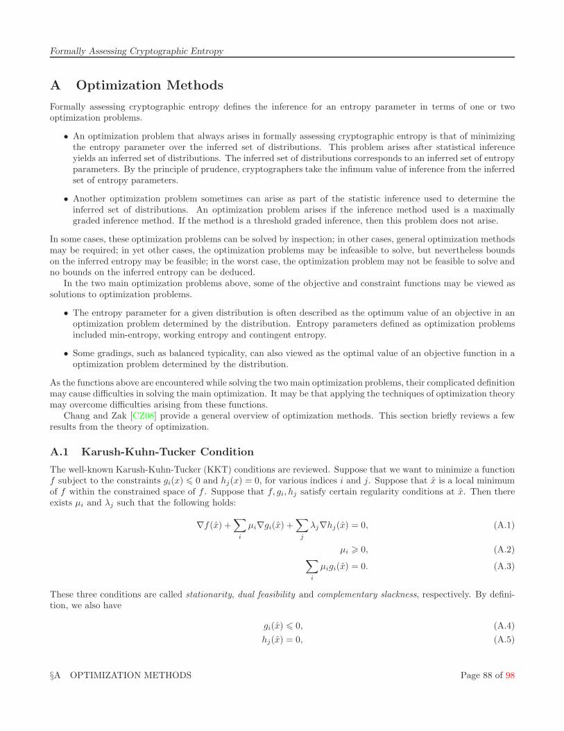
Formally Assessing Cryptographic Entropy
A Optimization Methods
Formally assessing cryptographic entropy defines the inference for an entropy parameter in terms of one or twooptimization problems.
• An optimization problem that always arises in formally assessing cryptographic entropy is that of minimizingthe entropy parameter over the inferred set of distributions. This problem arises after statistical inferenceyields an inferred set of distributions. The inferred set of distributions corresponds to an inferred set of entropyparameters. By the principle of prudence, cryptographers take the infimum value of inference from the inferredset of entropy parameters.
• Another optimization problem sometimes can arise as part of the statistic inference used to determine theinferred set of distributions. An optimization problem arises if the inference method used is a maximallygraded inference method. If the method is a threshold graded inference, then this problem does not arise.
In some cases, these optimization problems can be solved by inspection; in other cases, general optimization methodsmay be required; in yet other cases, the optimization problems may be infeasible to solve, but nevertheless boundson the inferred entropy may be feasible; in the worst case, the optimization problem may not be feasible to solve andno bounds on the inferred entropy can be deduced.
In the two main optimization problems above, some of the objective and constraint functions may be viewed assolutions to optimization problems.
• The entropy parameter for a given distribution is often described as the optimum value of an objective in anoptimization problem determined by the distribution. Entropy parameters defined as optimization problemsincluded min-entropy, working entropy and contingent entropy.
• Some gradings, such as balanced typicality, can also viewed as the optimal value of an objective function in aoptimization problem determined by the distribution.
As the functions above are encountered while solving the two main optimization problems, their complicated definitionmay cause difficulties in solving the main optimization. It may be that applying the techniques of optimization theorymay overcome difficulties arising from these functions.
Chang and Zak [CZ08] provide a general overview of optimization methods. This section briefly reviews a fewresults from the theory of optimization.
A.1 Karush-Kuhn-Tucker Condition
The well-known Karush-Kuhn-Tucker (KKT) conditions are reviewed. Suppose that we want to minimize a functionf subject to the constraints gi(x) 6 0 and hj(x) = 0, for various indices i and j. Suppose that x is a local minimumof f within the constrained space of f . Suppose that f, gi, hj satisfy certain regularity conditions at x. Then thereexists µi and λj such that the following holds:
∇f(x) +∑
i
µi∇gi(x) +∑
j
λj∇hj(x) = 0, (A.1)
µi > 0, (A.2)∑
i
µigi(x) = 0. (A.3)
These three conditions are called stationarity, dual feasibility and complementary slackness, respectively. By defini-tion, we also have
gi(x) 6 0, (A.4)
hj(x) = 0, (A.5)
§A OPTIMIZATION METHODS Page 88 of 98

Formally Assessing Cryptographic Entropy A.2 Optimizing Non-Smooth and Non-Continuous Functions
which together are called the condition of primal feasibility. These four conditions together are called the Karush-Kuhn-Tucker (KKT) conditions.
Under some further regularity conditions (see below), the Karush-Kuhn-Tucker (KKT) theorem states that theKKT conditions above are a necessary condition for x to be a local minimum x.
This suggests an algorithm for solving an optimization problem, as follows. Try to determine all x that either failthe regularity conditions or that meet the KKT conditions. The KKT theorem ensures that the local minima, andtherefore the global minima, must be among the set of all such x. If the set so obtained is finite, then its minimaare the global minima.
One regularity condition for the KKT theorem is as follows. The regularity condition has two parts. The firstpart is that all f and gi and hj are continuously differentiable. The second part is defined in terms of the activeconstraints, which includes all equality constraints and those inequalities constraints gi gi(x) = 0 at the solution xunder consideration. The condition is that the gradients of all the active constraints are linearly independent.
A.2 Optimizing Non-Smooth and Non-Continuous Functions
Min-entropy is generally not a smooth function of p. More precisely, it is only piece-wise smooth, and does not havea well-defined gradient at some points. Typical optimization methods, such as those employing the KKT conditions,use gradients. One approach to deal with the non-smoothness is to note that min-entropy may be viewed as theminimum of a number of smooth functions. Then one can optimize each such smooth function separately.
Generally, one is minimizing min-entropy over some inferred set of distributions (either a maximally graded orthreshold graded). In some cases, this inferred set of distributions is symmetric with respect to the entries of theprobability distribution vectors, so that it suffices to optimize just a single of the many smooth functions mentionedabove.
Typicality, such as inclusive or balanced typicality can not only be non-smooth, but can also be non-continuous.It may be possible to handle such non-continuous functions by breaking the optimization problem into multiple vari-ations, based on cases corresponding to each piece. As an alternative, this report has suggested forms of generalizedtypicality which can be chosen to be continuous and smooth, such as adjusted likelihood.
A.3 Model Constraints
A possible approach to handle the optimization problems arising from statistical inference, such as maximizing agrading or minimizing the entropy over a grading-thresholded set, is to parametrize the probability space Π usingone coordinate for each sample value x ∈ X . The x-coordinate at distribution p has value Pp(x).
This approach generally uses a lot of variables, say |X |, but may have the potential of simplifying the variousfunctions involved because the coordinates themselves already express the probabilities. So gradings such as likelihoodand typicality, and entropy parameters are expressible as certain coordinates, or sums of coordinates.
In this approach, the probability model would have to be described as a set of constraints on these coordinates.
Remark A.1. For an example, consider the (2, 2) independent model. The previously defined parametrization of the probabilityspace Π in this model was with two coordinates p0 and p1 with one equality constraint p0+p1 = 1 and two inequality constraintsp0, p1 > 0. It is also possible to parametrize this space with just a single coordinate, say p1, and get two inequality constraints:0 6 p1 6 1.
By model constraints, the space Π would instead by parametrized by four coordinates, which we may abbreviate top00, p01, p10, p11. For a system of constraints that describes Π, one can use
p00 + p01 + p10 + p11 = 1 (A.6)
p00, p01, p10, p11 > 0 (A.7)
p01 = p10 (A.8)
p00p11 = p01p10. (A.9)
§A OPTIMIZATION METHODS Page 89 of 98
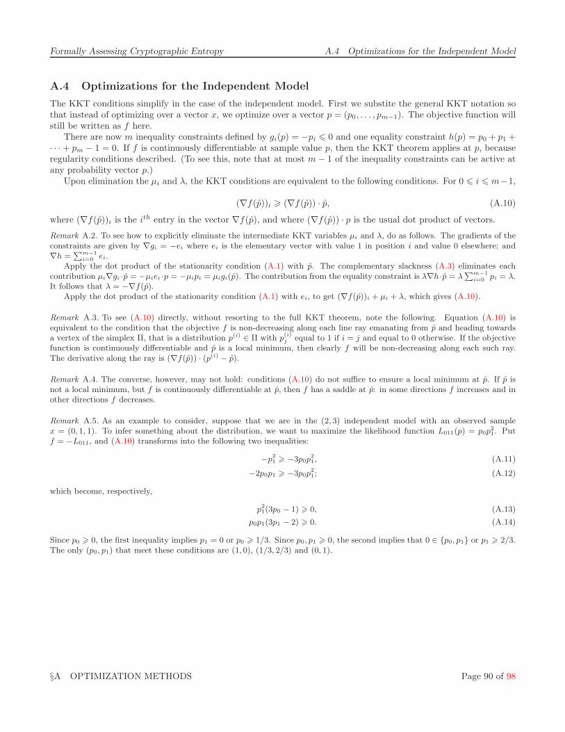
Formally Assessing Cryptographic Entropy A.4 Optimizations for the Independent Model
A.4 Optimizations for the Independent Model
The KKT conditions simplify in the case of the independent model. First we substite the general KKT notation sothat instead of optimizing over a vector x, we optimize over a vector p = (p0, . . . , pm−1). The objective function willstill be written as f here.
There are now m inequality constraints defined by gi(p) = −pi 6 0 and one equality constraint h(p) = p0 + p1 +· · · + pm − 1 = 0. If f is continuously differentiable at sample value p, then the KKT theorem applies at p, becauseregularity conditions described. (To see this, note that at most m − 1 of the inequality constraints can be active atany probability vector p.)
Upon elimination the µi and λ, the KKT conditions are equivalent to the following conditions. For 0 6 i 6 m−1,
(∇f(p))i > (∇f(p)) · p, (A.10)
where (∇f(p))i is the ith entry in the vector ∇f(p), and where (∇f(p)) · p is the usual dot product of vectors.
Remark A.2. To see how to explicitly eliminate the intermediate KKT variables µi and λ, do as follows. The gradients of theconstraints are given by ∇gi = −ei where ei is the elementary vector with value 1 in position i and value 0 elsewhere; and∇h =
Pm−1i=0 ei.
Apply the dot product of the stationarity condition (A.1) with p. The complementary slackness (A.3) eliminates eachcontribution µi∇gi ·p = −µiei ·p = −µipi = µigi(p). The contribution from the equality constraint is λ∇h·p = λ
Pm−1i=0 pi = λ.
It follows that λ = −∇f(p).Apply the dot product of the stationarity condition (A.1) with ei, to get (∇f(p))i + µi + λ, which gives (A.10).
Remark A.3. To see (A.10) directly, without resorting to the full KKT theorem, note the following. Equation (A.10) isequivalent to the condition that the objective f is non-decreasing along each line ray emanating from p and heading towardsa vertex of the simplex Π, that is a distribution p(i) ∈ Π with p
(i)j equal to 1 if i = j and equal to 0 otherwise. If the objective
function is continuously differentiable and p is a local minimum, then clearly f will be non-decreasing along each such ray.The derivative along the ray is (∇f(p)) · (p(i) − p).
Remark A.4. The converse, however, may not hold: conditions (A.10) do not suffice to ensure a local minimum at p. If p isnot a local minimum, but f is continuously differentiable at p, then f has a saddle at p: in some directions f increases and inother directions f decreases.
Remark A.5. As an example to consider, suppose that we are in the (2, 3) independent model with an observed samplex = (0, 1, 1). To infer something about the distribution, we want to maximize the likelihood function L011(p) = p0p
21. Put
f = −L011, and (A.10) transforms into the following two inequalities:
−p21 > −3p0p
21, (A.11)
−2p0p1 > −3p0p21; (A.12)
which become, respectively,
p21(3p0 − 1) > 0, (A.13)
p0p1(3p1 − 2) > 0. (A.14)
Since p0 > 0, the first inequality implies p1 = 0 or p0 > 1/3. Since p0, p1 > 0, the second implies that 0 ∈ {p0, p1} or p1 > 2/3.The only (p0, p1) that meet these conditions are (1, 0), (1/3, 2/3) and (0, 1).
§A OPTIMIZATION METHODS Page 90 of 98
Formally Assessing Cryptographic Entropy
B Modeling
This report concerns the task of formally assessing cryptographic entropy of a source. A prerequisite to this task isthat a probability model appropriate for the source has been selected. Selection of the model is not the main focusof this report. This section briefly describes approaches to selecting a probability model for a source. Two types ofapproaches are outlined below.
B.1 Relaxation Approach to Modeling
In the relaxation approach, one selects as an initial model a very restricted model. Either the restricted model couldbe selected as the ideal for the intended use of the source, such as being the uniform model, or as the model thathypothetically describes the source in most detail, such as a deterministic model. Next, one does hypothesis testingon the initial model, as outlined in §C. If the model is rejected, one must select another model. In the relaxationapproach, a relaxation of the initial model is selected. The choice of relaxation requires some inspiration or intuition.If one chooses the relaxation of the model before hypothesis testing, then one can do comparative hypothesis testing,which is the method preferred by this report. The relaxation approach can be iterated. Examples of the relaxationapproach to modeling are given in §6.5 and §6.6.
Section 6.5 deals with dice, and starts with an initial model which is the uniform model. It uses comparativehypothesis testing with the alternative model being the independent model. For one sample, it rejects the uniformmodel. In accordance with the relaxation approach to modeling, the model is relaxed from the uniform model tothe independent model, and then the independent model is tested. Again, comparative testing is used, with thealternative model being the Markov model. In this case, the independent model is accepted.
Section 6.6 deals with ring oscillators. It starts with an initial model in which the bit sequence produced by aring oscillator has a simple description determined by its frequency. In this case, the model has very low entropy,so the starting point is not the most optimistic one from the perspective of the source being used for cryptographicentropy. (It is optimistic from the perspective of an adversary.)
Two disadvantages of the relaxation approach are:
• The relaxation approach risks being over-optimistic, which could occur if, firstly, hypothesis testing yields afalse acceptance, meaning that the source has a distribution p which is not contained in the tested model, andif, secondly, the distribution p has significantly lower entropy than what would be inferred using the falselyaccepted model.
• In the event that a tested model is rejected, the relaxation approach provides no formally quantified guidanceon how to relax the probability model. The choice of relaxation is outside the scope of the formal techniquesin this report.
B.2 Restrictive Approach to Modeling
In the restriction approach to modeling, one starts from an initial relaxed model for the source. The selection ofthe initial model is based on intuition or inspiration, with the goal is of considering the current understanding ofthe source, and to capture all the possible ways in which the source could be described. The initial model should berelaxed, so making as minimal assumptions as possible.
Once the initial relaxed model (Π, X, P ) is formulated, a sample x from the source is gathered. Then inference isconducted using the formal methods described in this report. These inferences will depend on the observed sample.Say that that ∆ is the set of inferred distributions.
The restriction approach tries to derive a new model from the formal inference by restricting the initial model.The inference restriction would be to restrict the model to (∆, X, P ). The inference restriction is not really part ofthe restriction approach to modeling, for several reasons:
• It is really just doing inference, whereas the task at hand is modeling.
• For some inference methods, it is likely to be too restrictive. For example, if the initial model is the independnetmodel, and the inference method is maximal likelihood inference, then the restricted model will be singular.
§B MODELING Page 91 of 98

Formally Assessing Cryptographic Entropy B.2 Restrictive Approach to Modeling
• For some inference methods, the inferred set ∆ depends quite strongly the observed sample x, and the restrictedmodel (∆, X, P ), may be unnatural for the source.
So, the ideal restriction approach instead uses the inferred set of distrubitions ∆ as inspiration for some otherrestriction, say (Ξ, X, P ). Being a restriction Ξ ⊂ Π. Perhaps Ξ and ∆ have a large intersection. But Ξ should havea simpler description, and in particular, should not be defined in terms of the observed sample.
Any such restriction of the model must also be subjected to hypothesis testing. Comparative hypothesis testingusing the original model as the alternative may be applied. If the restricted model is accepted, then the process canbe iterated.
The relaxation and restriction approaches can be mixed. Indeed, they are not entirely different, since they bothinvolve steps of selecting models that are relaxed and restricted.
Remark B.1. In the restriction approach, one should start from a model that is relaxed but not too relaxed, otherwise theinferences may be too weak.
Remark B.2. For example, to model ring oscillators, one can gather multiple ring oscillators manufactured by the same process.For an initial relaxed model, one might model their outputs as independent from each other, and furthermore assume thateach has the same distribution. So, one is formulating the common power of the models. If one does not assume anythingabout each individual oscillator, then one essentially has the independent model. Considering the first 1024 output bits ofeach oscillator, then the initial model in the restriction approach is the (21024, 32) independent model.
The large width 21024 is due to the initial model not assuming anything about the first 1024 bits of the ring oscillator.The small length 32 is for the number of ring oscillators. Becuase length is much shorter than the length, the sample size isvery low. As such, the formal inferences may be so modest that the modeller should look directly at sample values themselvesshould for inspiration of how to hypothesize a restriction of the model.
Remark B.3. Remark B.2 uses an initial model that may be more relaxed than necessary. For example, it ignores the fact thatthe 1024 bits produced obtained from each ring oscillator sample are produced chronologically. It seems a mild assumptionthat the initial bits could not depend on the latter bits. So, a hidden Markov model could be hypothesized as an initial modelfor each individual oscillator. In this case, the formal initial model would be the common power of 32 copies of the hiddenMarkov model. The larger the size of the hidden state for the Markov model, the more relaxed the model would be.
In this the formal inference may provide more useful inspiration for modeling the source.
§B MODELING Page 92 of 98
Formally Assessing Cryptographic Entropy
C Hypothesis Testing
This report focuses on the task of formally assessing the cryptographic entropy of a source. As noted in §B, aprerequisite to assessing entropy is that a probability model appropriate for the source has been selected.
In this report, hypothesis testing means to determine the extent to which a given probability model is appropriatefor a given source. For example, extensive hypothesis testing may provide the confidence in the probability modelfor a given source, thereby providing confidence in entropy assessments for the source.
Hypothesis testing of a model on a source requires one to gather a sample value x from the source. Two types ofhypothesis testing are considered.
Hypothesis testing has the risk that the model can be falsely accepted. For example, if the model contains theuniform distribution, but the source is deterministic but pseudorandom, then it is unlikely to be rejected. In otherwords, a badly seeded cryptographic number generator would pass any general hypothesis test. The only way to trulyovercome this risk is to ensure that both hypothesis testing and cryptographic entropy assessment look at samplevalues drawn from the actual source of entropy, before any cryptographic processing.
C.1 Non-Comparative Hypothesis Testing
Non-comparative hypothesis testing does not rely on any other models. In the formalism of this report, one evaluatesthe maximal typicality of x, perhaps as induced by a sample statistic. If the maximal typicality of x is too low, thenone rejects the model. Some difficulties with non-comparative hypothesis testing are:
• The model has a probability of being falsely rejected, depending on the threshold for the maximal typicalityvalue used for rejection. In practice, this means setting the threshold very low. A concern with a low thresholdis that it enlarges the set of samples x that will lead to acceptance of the model. If the model is false, then alow threshold leads to a higher rate of false acceptance.
• The model may be subject to the tying effect, for example if the model contains subuniform distributions. Inthis case, rejection based on direct typiclity may be impossible for any x, because subuniform distributionsin the model mean x has typicality at least one half. As was seen earlier in the report, the tying effect canoften be overcome by using a tiebreaker sample statistic. Selecting an arbitrary sample statistic risks arbitraryhypothesis testing. Model-neutral sample statsitics may be used to avoid such arbitrariness, but model-neutralsample statistics are primarily motivated for making inferences, not for hypothesis testing.
• If the hypothesis model being tested is rejected, then one has no other model to assume, even though the sourcemay still have vital entropy.
C.2 Comparative Hypothesis Testing
In comparative hypothesis testing, the hypothesized model is tested against an alternative model which is relaxationof the hypothesized model. Comparative hypothesis testing is an attempt to address some of the difficulties withnon-comparative hypothesis testing.
In comparative hypothesis testing, one computes the maximal typicality of x using a sample statistic that ismodel-neutral with respect to the alternative model. One rejects the hypothesis if the maximal typicality obtainedis below some threshold. If the maximal typicality is below this threshold, then the hypothesized model is rejected.
The alternative model becomes the new hypothesized model. In comparative hypothesis testing, one can set thethreshold much higher than in non-comparative testing, because the cost of false rejection is only to relax the modelto the alternative model.
Because comparative hypothesis testing starts with two models, a hypothesized model and its alternative relax-ation, it may also provide some inspiration for modeling the source. On the one hand, if the hypothesis is accepted,then the hypothesized model can be further restricted in the direction it restricted the alternative model. In thiscase, the original hypothesis becomes the alternative, and comparative hypothesis testing can be applied again. Onthe other hand, if the hypothesis is rejected, then the old alternative model becomes the new hypothesized, and a
§C HYPOTHESIS TESTING Page 93 of 98

Formally Assessing Cryptographic Entropy C.2 Comparative Hypothesis Testing
new alternative model can be formulated by relaxing the old alternative model further in the direction that it relaxedthe old hypothesized model.
§C HYPOTHESIS TESTING Page 94 of 98

Formally Assessing Cryptographic Entropy
D Game-Theoretic Analysis
In this section, we consider a situation in which the adversary can choose the distribution p ∈ Π, and then triesto guess the sample value x drawn from p. This corresponds to the third level of adversary from Remark 2.5. Asnormal per the rest of this report, the entropy assessor retains the opporuntiy to make statistical inferences about pbased on an observed sample. The assessment can take the form of an inference of the entropy of p. Normally theassessed entropy would represent a bound on the adversary success rate at guessing the outcome of sample drawnfrom the distribution p. But in this section, the adversary has also chosen p. For example, the adversary could havechosen p with very low entropy. The goal of the assessor is to detect such a situtation and to properly account for it.If the assessor is correct, then either the key generation can be terminated, or more samples from the same or othersources can sample until an adequate amount of entropy is obtained. Consequently, selecting the lowest possibleentropy may not be the adversary’s optimal strategy, at least if the assessor is able to detect low entropy choices.Rather, an optimal strategy for the adversary may be to choose p with fairly low entropy, but also with the propertythat the assessor is likely to overestimate the entropy from an observed sample x.
Because both the adversary and the assessor adopt strategies, and the net result is a function of the strategies,(probabilistic) game theory is applicable.
For example, suppose that the cryptographic system is self-assesing using prospective inference. The first sampleis used for assessment, and the second for deployment. Assume that the two samples so obtained are independentand identically distributed. So, the overall source model is a common square (Π, X2, R), see §2.4.5 of the model(Π, X, P ) for a single sample. The game works as follows:
1. The adversary chooses p ∈ Π.
2. A sample (x1, x2) is drawn in the model (Π, X2, R).
3. The assessor is given x1.
4. The assessor outputs an entropy estimate H ∈ R.
5. The adversary guesses a value y.
6. If y = x2, the score of the game is s1(H).
7. If y 6= x2, the score of the game is s0(H).
The assessor tries to maximize the score, while the adversary tries to minimize the score. The strategies of theassessor and the adversary in this game depend on the scoring function s0, s1 : R → R.
Indeed, the game can be viewed as a two-player game in which the two players make choices simultaneously. Theadversary’s choice consists of the pair (p, y), a distribution and a sample value. The assessor’s choice consists of aentropy assessment function H : X → R. The score of the game is then a random variable, taking values in R.Although the range of the score is a continuum, the random variable is discrete if the set X is finite. The probabilitythat a score results in s is
Pp(y)
∑
x:s=s1(H(x))
Pp(x)
+ (1 − Pp(y))
∑
x:s=s0(H(x))
Pp(x)
. (D.1)
The adversary wishes to minimize the score, while the assessor wishes to maximize the score. But since the score isa random variable, not a single quantity, maximization and minimization of the score are not clearly defined.
A simple way to define what it means to optimize of a random variable is to optimize its expected value. This maybe too simplistic for cryptographic applications, because expected values are often not appropriate considerationsfor cryptography. Nevertheless, suppose that both the adversary and the assessor attempt to optimize (in differentdirections) the expected value of the score. The expected value of the score is
∑
x∈X
Pp(x) (Pp(y)s1(H(x)) + (1 − Pp(y))s0(H(x))) . (D.2)
§D GAME-THEORETIC ANALYSIS Page 95 of 98

Formally Assessing Cryptographic Entropy
The summation index x corresponds to the observed value x1 in the step-by-step game above.For concreteness, suppose that (Π, X, P ) is the (2, 3) independent mode. Simple, but arguably arbitrary, choices
for the scoring functions are s0(h) = h and s1(h) = −h. The optimization objective function for both players, namelythe expected score, simplifies to:
1 − 2Pp(y)∑
x∈X
Pp(x)H(x). (D.3)
In cryptographic applications, the assessor’s only source of randomness is the source. So, effectively, we can assumethat the assessor must fix the choice of assessment function H . In game theory terminology, the assessor is forcedto use a pure strategy. The adversary may use a mixed strategy. For example, the choice of (p, y) in the game maynot be fixed, but actually drawn from a distribution.
The next step would to be apply the techniques of game theory to determine optimal strategies for the cryptog-rapher and the adversary. The optimal assessment strategy depends on the model, the choice of scoring function,and the definition of the objective functions obtained from the random score variable.
§D GAME-THEORETIC ANALYSIS Page 96 of 98

Formally Assessing Cryptographic Entropy
E Estimation Theory
Estimation theory is an approach to statistical inference that takes a given inference method, and produces anevaluation of its quality.
For example, suppose that (Π, X, P ) and r : Π → R is a parameter, and that i : X → R is a inference function.Furthermore, suppose that the space R is a convex space, in the sense that convex combinations are defined in R.Then the inference function i is said to be an unbiased estimator for r if, for all p ∈ Π, it is true that
E(i(x)) = r(p), (E.1)
where E is the expected value of i(x) according to the probability distribution p. This means that:
E(i(x)) =∑
x∈X
Pp(x)i(x). (E.2)
Remark E.1. The min-entropy parameter H∞ is a non-polynomial function of p ∈ Π. The left hand side of (E.1) is apolynomial function in p, as seen by the definition (E.2). Therefore, for almost all choices of Π, no inference function is anunbiased estimator for H∞.
Remark E.2. The maximum likelihood estimate (inference) is an unbiased estimator for the probability distribution p itself inthe unrestricted model.
Remark E.3. Suppose that we have two models (Π, X, P ) and (Π, Y, Q), with a shared probability space. Suppose we haveprobability parameters r : Π → R and s : Π → S and inference functions i : X → R and j : Y → S. Recall that we defined theproduct model (Π, X×Y,P×Q) such that (P×Q)p(x, y) = Pp(x)Qp(y). Similarly, we may define the product of the parametersr × s : Π → R × S : p 7→ (r(p), s(p)) and the product of the inference functions i × j : X × Y → R × S : (x, y) 7→ (i(x), j(y)).Then r× s is a parameter for the product model and i× j is an inference function for the product model with the same rangeas the product parameter, namely R× S. If i and j are unbiased estimators for r and s respectively, then i× j is an unbiasedestimator for r × s.
Remark E.4. The maximum likelihood inference function is an unbiased estimator of the probability distribution itself in the(m, N) independent model. It is easy to see that the maximum likelihood inference function i is defined such that i(x) = f(x),where f is the frequency vector of the sample vector x. This means that f(x)i = j/N if the number of k such that xk = i isj. To show that this is unbiased, by symmetry, it suffices to show that the expected value of f(x)0 is p0. The expected valueof f(x)0 is
f(x)0 =X
x0,x1,...,xN−1
px0px1 . . . pxN−1 |{k : xk = 0}| /N
= 1N
X
x0,x1,...,xN−1
p0∂
∂p0px0px1 . . . pxN−1
= 1N
p0∂
∂p0
X
x0,x1,...,xN−1
px0px1 . . . pxN−1
= 1N
p0∂
∂p0(p0 + · · · + pm−1)
N
= 1N
p0N(p0 + · · · + pm−1)N−1 ∂p0
∂p0
= p0,
(E.3)
where the pi are treated as indeterminates when calculating partial derivatives, and then treated again as probabilities in thefinal steps. The sums are over x ∈ X, meaning 0 6 x0, . . . , xN−1 6 m − 1, with the xi ∈ Z.
Other quality measures of the estimator can be defined given a metric d on the space R. For each p, we can definethe error of i as an estimator of r:
ǫe(p, i, r) = E(d(i(x) − r(p))e), (E.4)
§E ESTIMATION THEORY Page 97 of 98

Formally Assessing Cryptographic Entropy
where e would typically be one or two. However, in statistical inference, p is unknown. Therefore, so is the errorabove. What one can do is take the maximum error over all p as the total error of the inference i of r. Or, instead,if Π is equipped with a measure, take the average error over Π.
These notions suggest that one can define an inference function in terms of achieving best quality. For example,perhaps choose an unbiased estimator, if possible. Generally, among the remaining choices, choose an inferencefunction that produces the least total error, or average error.
Remark E.5. The suitability of estimation theory for cryptology is unclear, primarily because of Remark E.1.Furthermore, all the estimation methods above use expectation, and thus use averages over the sample space X. It is a
theme of cryptology that danger lurks in using averages, because an adversary, unlike a natural process, will not confine itselfto random behavior, and thus to average behavior. An adversary will search over the sample space X, so averages over samplespace X may not be a good measure of anything.
§E ESTIMATION THEORY Page 98 of 98