Formality and geometric structures

Bjarne Kosmeijer

a thesis submitted to the Department of Mathematics

at Utrecht University in partial fulllment of the requirements for the degree

of

Master in Mathematics

supervisor: Dr. Gil Cavalcanti

June 14, 2018

Contents

Introduction 2

Overview 4

1 Dierential graded algebras 6

1.1 Denition . . . . . . . . . . . . . . . . . . . . . . . . . . . . . . . . . . . . . . . . . . . . . . 6

1.2 Minimal models . . . . . . . . . . . . . . . . . . . . . . . . . . . . . . . . . . . . . . . . . . . 8

1.3 Sullivan algebras . . . . . . . . . . . . . . . . . . . . . . . . . . . . . . . . . . . . . . . . . . 11

1.4 Relative algebras and models . . . . . . . . . . . . . . . . . . . . . . . . . . . . . . . . . . . 15

1.5 Formal algebras . . . . . . . . . . . . . . . . . . . . . . . . . . . . . . . . . . . . . . . . . . . 16

1.6 Characterizing formality . . . . . . . . . . . . . . . . . . . . . . . . . . . . . . . . . . . . . . 18

2 Rational homotopy theory and CDGA's 26

2.1 Simplicial objects and APL . . . . . . . . . . . . . . . . . . . . . . . . . . . . . . . . . . . . . 26

2.2 Comparing APL(M ;R) and Ω(M) . . . . . . . . . . . . . . . . . . . . . . . . . . . . . . . . . 29

2.3 Minimal models and homotopy groups . . . . . . . . . . . . . . . . . . . . . . . . . . . . . . 32

2.4 Spatial realization . . . . . . . . . . . . . . . . . . . . . . . . . . . . . . . . . . . . . . . . . . 34

2.5 Spaces and CDGA's, pushouts and pullbacks . . . . . . . . . . . . . . . . . . . . . . . . . . 38

3 Formality & geometric structures: rst examples 44

3.1 Kähler manifolds . . . . . . . . . . . . . . . . . . . . . . . . . . . . . . . . . . . . . . . . . . 44

3.2 Lie groups and symmetric spaces . . . . . . . . . . . . . . . . . . . . . . . . . . . . . . . . . 46

3.3 Formality and harmonic forms . . . . . . . . . . . . . . . . . . . . . . . . . . . . . . . . . . . 49

3.4 Special holonomy . . . . . . . . . . . . . . . . . . . . . . . . . . . . . . . . . . . . . . . . . . 50

4 Formality of quaternionic Kähler manifolds 53

4.1 Quaternionic Kähler geometry . . . . . . . . . . . . . . . . . . . . . . . . . . . . . . . . . . . 53

4.2 Formality of brations . . . . . . . . . . . . . . . . . . . . . . . . . . . . . . . . . . . . . . . 54

4.2.1 Elements of spectral sequences . . . . . . . . . . . . . . . . . . . . . . . . . . . . . . 54

4.2.2 Relative ltered models . . . . . . . . . . . . . . . . . . . . . . . . . . . . . . . . . . 58

4.2.3 S2n-bundles . . . . . . . . . . . . . . . . . . . . . . . . . . . . . . . . . . . . . . . . 60

4.2.4 Proof of Theorem 4.23 . . . . . . . . . . . . . . . . . . . . . . . . . . . . . . . . . . 62

5 Formality and Mayer-Vietoris 65

5.1 Examples of G2-manifolds . . . . . . . . . . . . . . . . . . . . . . . . . . . . . . . . . . . . . 65

5.2 s-formality . . . . . . . . . . . . . . . . . . . . . . . . . . . . . . . . . . . . . . . . . . . . . . 66

5.3 Building formal manifolds by gluing . . . . . . . . . . . . . . . . . . . . . . . . . . . . . . . 71

5.4 Formality and deleting submanifolds . . . . . . . . . . . . . . . . . . . . . . . . . . . . . . . 78

Outlook and conclusion 83

A Appendix on dierential geometry 84

A.1 Connections & parallel transport . . . . . . . . . . . . . . . . . . . . . . . . . . . . . . . . . 84

A.2 Riemmanian manifolds & Levi-Civita connection . . . . . . . . . . . . . . . . . . . . . . . . 85

A.3 Hodge theory of a Riemmanian manifold . . . . . . . . . . . . . . . . . . . . . . . . . . . . . 85

B Appendix on topology 87

B.1 Denitions of homotopy, homology and cohomology . . . . . . . . . . . . . . . . . . . . . . . 87

B.2 Connections between homotopy, homology and cohomology . . . . . . . . . . . . . . . . . . 88

1

Introduction

Suppose we are given a pair of manifolds (or more generally topological spaces, or homotopyclasses of spaces), and we are interested in ways to distinguish them from each other. Ofcourse we have dierent ways to do this, for instance: the homotopy groups, the (singular)homology, or the deRham-cohomology.

manifoldsM

tt **

homotopy groupsπi(M)

singular homology

Hi(M ;Z)

deRham cohomology

H idR(M)

But although the homotopy groups have a high theoretical value (they are very geometricallydened and hence are really useful if one wants information about basic geometry of thespace), apart from π1 they are notoriously hard to calculate, even in the easiest exampleslike the sphere. On the other hand the homology and cohomology groups are quite easy tocalculate (there are gadgets like excision, Mayer-Vietoris and an actual full description of thevalues on spheres), but we lose a certain theoretical value (surely one can use it to distinguishspaces, but what does an element of the homology group represent geometrically?). So it isa natural question to ask whether there are ways to retrieve information on the homotopygroups from (co)homology. The most important example is a quite fundamental result byHurewicz.

Theorem 0.1 (Hurewicz) The rst non-zero πi(M) and rst non-zero Hi(M ;Z) (i > 0)occur at the same index, and for this index n the Hurewicz map πn(M)→ Hn(M ;Z) is anisomorphism (if n 6= 1) and an isomorphism (π1(M))ab → H1(M ;Z) (if n = 1).

We can also connect homology and cohomology of a manifold, like Poincare duality and theuniversal coecient theorem

Theorem 0.2 (Poincare duality) IfM is an oriented closed n-dimenisonal manifold thenHkdR(M) ∼= Hn−k(M ;R).

Theorem 0.3 H idR(M) ∼= HomZ(Hi(M,Z),R)

So we're in the following situation:

manifolds M

zz

%%

singular homology

Hi(M ;Z)

jj

PD, UCT

**

homotopy groups πi(M)tt

Hurewicz

44

deRham cohomology H idR(M)

2

We should note however, that the Hurewicz theorem stops giving information at an earlystage (indeed it only connects the rst non-zero entries), and we would like to have anarrow going to all the homotopy groups, not just the rst non-trivial one. This may be toooptimistic, but if we restrict to only the torsion free part, and insert the full deRham-complexin the middle, Sullivan [22] provided us with a way to go.

manifoldsM

$$deRham cplx

Ω(M)

&&

Sullivan `73ss

rational h'topyπi(M)⊗Q

deRham coh'logy

H idR(M)

M formal?oo

Now, ideally we would like an arrow from the deRham cohomology to the rational homotopythat gives us roughly the same result as going directly from the deRham complex to therational homotopy. This is what will be called formality of M , and will be our main topic.It turns out that one can use geometric structures to deduce that certain classes of mani-folds are formal. This leads to two justications for trying to nd formal (and non-formal)manifolds: rstly the rational homotopy of formal manifolds is fully contained in the co-homology, making them interesting from a topological point of view, and secondly the factthat admitting a certain geometrical structure can imply formality, showing that a manifoldis not formal is an ecient way to prove that it can not admit certain structures.

In the rst part of the text we will be setting up the language to formulate (and give asketch of the proof) of the theorem by Sullivan. After that, starting with Kähler manifolds,we will discuss a few types of geometric structures that are interesting with respect to for-mality. The discussion of a few of these structures will be used as a starting point for certainmore broad theorems which will (or at least try to) solve the formality question.

3

Overview

The thesis will be structured as follows.

In Section 1 we will set up the theory of dierential graded algebras, starting with thedenition and some basic examples (Section 1.1). From one of the examples we will denethe notion of a minimal algebra and minimal models (Section 1.2), which replaces an algebraby a more workable one which shares important properties. In this part we will also makeprecise the theorem of Sullivan.To settle some technical question (for instance showing the uniqueness of minimal models),we will also discuss Sullivan algebra (Section 1.3) and relative algebras (Section 1.4). In theend we will encounter a class of algebras which has preferable properties with respect tominimal models and cohomology, namely formal algebras (Section 1.5). A goal of the textis to nd ways to distinguish formal algebras and formal manifolds (manifolds M for whichΩ(M) is a formal algebra) from the non-formal ones. As a start we describe some algebraiccharacterizations of formality (Section 1.6).

The theory of CDGA's is well understood in the context of rational homotopy theory, inthat there is a one-to-one correspondence between rational homotopy types and isomorphismclasses of minimal algebras. We will discuss elements of this in Section 2. For instance wewill describe a topological counterpart to de Rham complex (Section 2.1), and show that thealgebraic theory of it is equivalent to the one of the deRham complex (Section 2.2). Usingthis broader point of view we will give a sketch of the proof of Sullivan's result (Section 2.3).The topological viewpoint allows to not only make algebraic models out of spaces, but alsomake spaces out of algebraic models (Section 2.4), which we will use to show that passingto the algebraic models preserves pushout-like properties (Section 2.5).

One of the main goals is to formulate formality of manifolds in terms of geometric structuresthat a manifold can admit. Indeed using the dierential algebra that comes with certaingeometric structures, one can massage the deRham-complex to show that it is formal. InSection 3 we will give some examples of this. The prototypical example are Kähler mani-folds, and we will describe a result by Deligne, Griths, Morgan and Sullivan [5] that showthat Kähler manifolds are formal, using the so-called ddc-lemma (Section 3.1). We will alsoshow that Lie groups are formal, and the proof of this generalizes to show that all symmetricspaces are formal (Section 3.2). An alternative proof of this fact leads us to the notion ofgeometrical formality, which deals with the connection of harmonic forms as formality. Wewill briey discuss this notion, and show that it is a far stronger notion which comes with afew obstructions (Section 3.3).We will end this section by describing the path along we will pursue our search of geomet-ric structures that induce formality. In particular we introduce (Section 3.4) the notion ofspecial holonomy, which gives us a short list of geometric structures that are central in ourdiscussion.

Following this path, we rst discuss quaternionic Kähler manifolds in Section 4. We do

4

this in two parts, rst doing some geometry in Section 4.1, to show that a quaternionicKähler manifold is the base of a bration with formal total space and formal ber (namelyS2). With this we then look at a result of Amman and Kapovitch [1] concerning brationswith formal ber (Section 4.2), discussing both the proof in the general case (in which weleave some black boxes concerning spectral sequences), and proving it in the case where theber is an even dimensional sphere.

Then after quaternionic Kähler manifolds come Joyce-manifolds (or also G2-manifolds). Wewill not discuss a proof that all Joyce-manifolds are formal (at the moment such a proofis not known to the author). What we will do is mention a few papers describing waysto mass produce Joyce-manifolds (Section 5.1) and discuss the central feature that theseconstructions have. In particular they produce manifolds that come around as the gluing oftwo formal manifolds along a formal intersection. Because of this we will use Section 5 todiscuss formality of manifolds that arise in this way.We start by using Poincaré duality to greatly simplify the question of formality for orientable(in particular simply connected) manifolds (Section 5.2). With this at hand we present newresults, showing that together with a simple cohomological condition gluing formal manifoldsalong a formal intersection yields a formal manifold (Section 5.3).The prototypical use of the theorem is showing that the connected sum of two formal mani-folds is formal. In order to use our new result, we rst need to show that M\∗ is formal ifM is (which we will do). To generalize this further we will nish by presenting some partialresults to the question whether M\S is formal if M is formal (Section 5.4).

5

1 Dierential graded algebras

1.1 Denition

As mentioned in the overview we want to develop an algebraic language in which to dotopology. To this end we set up the theory of dierential graded algebras. The language isaimed to put the usual deRham-complex of dierential forms (or equivalently the algebraof rational forms of any topological space) in a general framework, as to eectively extractalgebraic data out of them. With the deRham-complex in mind, we dene them as follows:

Denition 1.1

a) A vector space V is called a graded vector space if there are linear subspacesV ii∈N such that V = ⊕i∈NV i. The element v ∈ V i are called homogeneous ofdegree i, the latter of which is denoted by |v| = deg(v) = i.

A morphism between graded vector spaces V and W is a linear map f : V → Wsuch that f(V i) ⊂ W i.

b) A graded vector space A which carries an algebra structure is called a gradedalgebra if V i · V j ⊂ V i+j.

A morphism between two graded algebras A and B is a linear map φ : A → Bwhich is both a morphism of graded vector spaces and a morphism of algebras(i.e. φ(a) · φ(b) = φ(a · b)).

c) A graded algebra is called commutative if ab = (−1)|a||b|ba for a and b homogeneouselements.

Passing from maps of graded algebras to commutative graded algebras we do notpose any more properties on them (indeed we don't add structure to preserve).

d) A graded vector space V is called a cochain complex if there is a linear mapd : V → V s.t. d(V i) ⊂ V i+1 subject to the relation d2 = 0. The elements inker(d) are called closed, while elements in im(d) are called exact.

A morphism of cochain complexes (V, dV ) and (W,dW ) is a linear map f : V → Wsuch that dW f = f dV .

e) A cochain complex A which also is a graded algebra is called a dierential gradedalgebra (DGA) if d(ab) = d(a)b+ (−1)|a|ad(b) (the Leibniz identity) for all homo-geneous a and b.

A morphism between two DGA's A and B is a linear map φ : A→ B that is botha morphism of cochain complexes and a morphism of graded algebras.

f) A dierential graded algebra which is commutative as a graded algebra is calleda commutative dierential graded algebra (CDGA)

6

Just as going from graded algebras to commutative graded algebras, we do notpose new properties when going from maps of DGA's to maps of CDGA's.

Remark 1.2 This denition can be phrased for vector spaces over any eld. Since we'remostly interested in deRham-complexes of manifolds, in this section we will work out thetheory for vector spaces over R, but everything works verbatim for any eld of characteristic0. In the next chapter we will delve a bit into rational topology, hence there most thingswill be dened over Q.

Now resembling the familiar procedure of going from singular (co)chains to singular (co)homo-logy or going from the deRham-complex to deRham-cohomology, we can take the cohomologyof a cochain complex.

Denition 1.3 Given a cochain complex (A, d) we can construct the graded vector spaceH(A, d), called the cohomology of (A, d), setting:

H i(A, d) =ker(d : Ai → Ai+1)

im(d : Ai−1 → Ai)

Note that d factors to the cohomology, where it vanishes for obvious reasons. In particularwe get (H(A, d), 0) ∈ Ch≥0. Further even, any addional structure we have put on (A, d)descends to one on H(A, d). Indeed, an algebra structure on (A, d) that is compatible withd (i.e. satises Leibniz), descends to H(A, d) (precisely because of Leibniz), and H(A, d) iscommutative if (A, d) is. Furhermore any cochain map f : (A, d) → (B, d) induces a mapH(f) = f ∗ : H(A, d) → H(B, d), also preserving any additional structure. This establishesH as a functor from Ch≥0 to Ch≥0, restricting to one from dga to dga and one from cdgato cdga in a canonical way, and in the following we will interpret the cohomology of a CDGAalways as a CDGA in its own right.

Throughout this text we will encounter the notion of `nite type' algebras and spaces. Withthe denition of cohomology in hand we can make precise what we mean by that:

Denition 1.4 A CDGA (A, dA) is called of nite type if H(A, dA) is nitely generated asalgebra (in particular H i(A, dA) is always nite dimensional). A space X is called of nitetype if H i(X;Q) is nite dimensional for all i (note that for most spaces the cohomologyis trivial after some nite degree, so in that case we get that H(X;Q) is also nitelygenerated).

The notion of cohomology also enables us to dene an important class of morphisms, namelythe quasi-isomorphisms.

Denition 1.5 A map f : (A, d)→ (B, d) of chain complexes (or DGA's, or CDGA's) is aquasi-isomorphism if H(f) : H(A, d)→ H(B, d) is an isomorphism.

Now that we have the abstract framework in position, we t deRham-complex in it:

7

Example 1.6 For a manifold M , the deRham-complex Ω(M) together with the wedgeproduct and the exterior derivative becomes a CDGA. Furthermore, for any smooth mapF : M → N , the pull-back F ∗ : Ω(N)→ Ω(M) becomes a morphism of CDGA's.Furthermore any homotopy equivalence (and even any weak homotopy equivalence) inducesa quasi-isomorphism.

Example 1.7 Fix a volume form α ∈ Ωn(Sn) and consider the map φ : H(Sn) = span(1, [α])→Ω(Sn) sending 1 to the constant function 1 ∈ Ω0(Sn) and sending [α] to α. This map thenis a quasi-isomorphism between H(Sn) and Ω(Sn).

Example 1.8 Suppose we are given a graded vector space V . We can then form the freeCGA ΛV dened by taking the quotient of the tensor algebra by relations of the forma ⊗ b − (−1)ijb ⊗ a where a ∈ V i and b ∈ V j (i.e. we only impose relations to make ΛVgraded commutative). Note that as an algebra ΛV = Symmetric(V even)⊗ Exterior(V odd).Of course, together with a map d : ΛV → ΛV , satisfying d2 = 0 and Leibniz, ΛV becomesa CDGA. The important remark here is that, since an element in ΛV is a polynomial inelements of V , by Leibniz any dierential is induced by its restriction d : V → ΛV .Given a basis xi of V , we will sometimes build up ΛV with only information about thexi's. Indeed given a set xi together with |xi| ∈ N and d(xi) a polynomial in the elementsof xi such that everything works out (i.e. the degree of dxi adds up to |xi|+ 1, imposingLeibniz d2 becomes zero, et cetera), the structure of ΛV for V = span(xi) is xed.

Remark 1.9 To add to the last point made, from time to time we will be a bit sloppy withnotation in the case that we have a basis for V . Then we will sometimes not write ΛV or(ΛV, d) but something like Λxi or 〈xi; |xi| = ..., dxi = ...〉.

1.2 Minimal models

Having the language of free objects as described in the last example, we can dene anotherimportant class of CDGA's, the minimal ones:

Denition 1.10 A CDGA (ΛV, d) as described above is called minimal if

V = ⊕n≥1Vn (i.e. V 0 = 0) and d(V ) ⊂ Λ≥2V (where Λ≥2 means wedges of length

at least 2).

V admits a homogeneous basis vα indexed by a well-ordered set such that |vα| ≤ |vβ|if α ≤ β and dvα ∈ Λvββ<α.

Remark 1.11 Most of the time we will restrict to algebras for which H1 vanishes, whichfor minimal algebras translates to V 1 = 0. Then the second point is vacuous. To see this,note that if we have a homogeneous basis of V , ordered by degree, for a v in this basis|dv| = |v|+ 1. Since there are no elements of the basis of degree 1, this means that dv is aproduct of elements of degree smaller than the degree of v.So since we will only work with simply connected algebras, we will ignore the second part

8

in what follows (although in the general setting we should really not forget about it!).

The nomenclature of the word minimal here is explained by the fact that the second statementimplies that none of the generators is exact, hence we have a minimal number of generatorsneeded to generate the cohomology.

Denition 1.12 Given a CDGA A, a minimal model for A is a minimal algebraM togetherwith a quasi-isomorphism φ : M → A.

So a minimal model of A is somehow a way to encode all the relevant information of A with aminimal amount of algebraic relations. Note also that since φ has to be a quasi-isomorphism,we get that H0(A) = R. Any CDGA with this property is called connected.

Example 1.13 Consider the odd-dimensional sphere S2n−1 with a volume form α. Wedene ΛV with as generating set one element v in degree 2n − 1 with dv = 0. Note thatsince the order of v is odd, we have ΛV = span(1, v). Then dening φ : (ΛV, d)→ Ω(S2n−1)by φ(v) = α, we get a quasi-isomorphism, establishing (ΛV, d) as a minimal model ofΩ(S2n−1).

Example 1.14 Now consider even-dimensional the sphere S2n with a volume form α. Ifwe do the same as before we get the right cohomology up to degree 4n − 1, but notethat since now the order of v is even, ΛV becomes a polynomial algebra on v with zerodierential, hence ΛV also has cohomology in degree 4n, 6n, 8n, et cetera generated by v2,v3 and v4 respectively. To cope with this problem we articially make v2 exact, by settingan extra generator w in degree 4n − 1, together with dw = v2 and φ(w) = 0 (from thispoint on in this example we have V = spanv, w). Then φ : (ΛV, d)→ Ω(S2n) becomes aquasi-isomorphism, and we have a minimal model for Ω(S2n).

Example 1.15 If one considers the cohomology algebras H(Sn) of the spheres, and triesto nd minimal models for them, it dawns that the result is the same. This is no coinci-dence. Indeed for such a minimal model ψ : M → H(Sn), composing with the map φ fromExample 1.7 we get a minimal model φψ : M → Ω(Sn) for Ω(Sn). In the next theorem wewill show uniqueness of minimal models, so it was to be expected that the minimal modelscoincide.

Example 1.16 We recall that H(CP n) = R[α]/(αn+1) with α = [ω] for some symplecticform ω ∈ Ω2(CP n) (for instance the Fubini-Study form). So if we want to make a minimalmodel of Ω(CP n) we rst need a closed generator v in degree 2, but then d(vn+1) = 0. Hencewe need to make vn+1 exact, thus we add a generator w in degree 2n + 1 with dw = vn+1.Then setting φ(v) = ω and φ(w) = 0 yields a quasi-isomorphism φ : (ΛV, d) → Ω(CP n)which is the minimal model of Ω(CP n).

Now one might wonder whether all CDGA's admit a minimal model, and, if they do, howmany. The rst question is always answered positively, while it may happen that there areCDGA's with multiple non-isomorphic minimal models. Both to have a simpler proof of therst fact, while also having an unique minimal model, we restrict to CDGA's A such that

9

H1(A) = 0, these are called simply connected.

Theorem 1.17 Let A be a simply connected CDGA,

a) There is a minimal model φ : M → A of A.

b) If there are two minimal modes M1φ1−→ A

φ2←− M2 of A, there is an isomorphismψ : M1 →M2 such that φ1 ' φ2 ψ.

Remark 1.18 The notion of homotopy that we refer to in the second part of the theoremwill be dened in the next section. Also we will prove the second part of the theorem onlyin the next section.

Proof. At this point we only prove existence. We construct models φ : (ΛV, d) → A with(ΛV, d) minimal such that H i(φ) is an isomorphism for 0 ≤ i ≤ n, in such a way that weget from the n-step to the (n+ 1)-step by adding a few extra elements to V in degree n andn+ 1. Then taking the union of all these additions (or equivalently one can take the directlimit under the inclusions) we get a minimal model for A.

We can make the induction basis for any of n = 0, n = 1 or n = 2, but we'll settle onthe last case. In that case we set V 2 = H2(A), with d = 0, and φ : ΛV → A such that[φ(v)] = v for all v ∈ V 2 (i.e. nd a section of A2 ∩ ker d→ H2(A)).

Then suppose we have φ : ΛV → A up to the point that H i(φ) is an isomorphism forall 0 ≤ i ≤ n. We look at Hn+1(φ), and if it is not an isomorphism already we have to arti-cially make it surjective and injective. To this end we add generators W to V , by settingW n = ker(Hn+1(φ)) and W n+1 = coker(Hn+1(φ)). We set d|Wn+1 = 0 and d|Wn in such away that d(w) ∈ (ΛV )n+1 is a generator of w ∈ Hn+1(ΛV ). Furthermore we extend φ to W n

in such a way that φ(d(w)) = dA(φ(w)). This is possible since H(φ)(w) = 0 and hence forthe representative dw of w we have that φ(dw) = dA(a), where a can be chosen to dependlinearly on w, and we set φ(w) = a. To end we dene φ|Wn+1 : W n+1 → An+1 ∩ ker dA asection of An+1 ∩ ker dA → Hn+1(A)→ cokerHn+1(φ).

At this point it is straightforward to check that H i(φ) is an isomorphism for i ≤ n + 1.To see this note that we don't add closed or exact elements in Λ(V ⊕W ) in degree ≤ nso the extended φ satises that H i(φ) is an isomorphism for 0 ≤ i ≤ n simply because theoriginal φ is. On the other hand by construction Hn+1(φ) becomes an isomorphism.

The important result by Sullivan, as announced in the introduction, is the following:

Theorem 1.19 (Sullivan `73) Let M be a simply connected manifold. Let φ : ΛV →Ω(M) be the minimal model of Ω(M). There is a bilinear non-degenerate pairing V k ×(πk(M)⊗R)→ R, in particular the rank of πk(M)⊗R as an R-vector space (or equivalentlythe rank of πk(M)⊗Q as a Q-vector space) equals the number of generators of V in degreek.

10

This theorem has a far-reaching implication on the calculation of the rational homotopygroups of manifolds. Normally when you want to do this, one needs to do calculations withthe Postnikov tower of the manifold, which tends to be quite a nasty job. Instead when onehas a grip on the deRham-complex of the manifold, calculating the minimal model is a fareasier task. Essentially the theorem states that the information contained in the deRham-complex is the same as in the rational Postnikov-tower, and therefore it doesn't come as asurprise that this pops up in the proof (which we will not discuss at this time).

Combining the theorem with Examples 1.13, 1.14 and 1.16 one concludes:

Corollary 1.20

πi(S2n)⊗Q =

Q if i = 2n, 4n− 10 else

πi(S2n−1)⊗Q =

Q if i = 2n− 10 else

πi(CP n)⊗Q =

Q if i = 2, 2n+ 10 else

1.3 Sullivan algebras

We still want to have a feasable language to proof the uniqueness of the minimal model.Sullivan algebras do this for us, and hence we digress for a bit in that direction. This willyield a proof of the uniqueness of the minimal model, and also gives us a few other interestingresults on the side. We closely follow chapter 12 of the book by Félix, Halperin and Thomas[7].

Denition 1.21 A Sullivan algebra is a CDGA of the form (ΛV, d) where:

a) V = ⊕p≥1Vp

b) There are subspaces V(i) of V such that V(0) ⊂ V(1) ⊂ · · · ⊂ V = ∪∞i=0V(i) such that dmaps V(k) into ΛV(k−1) (and in particular d = 0 on V(0)).

Further, a Sullivan model of a CDGA A is a quasi-isomorphism φ : ΛV → A with ΛV aSullivan algebra.

Clearly any minimal CDGA is a Sullivan algebra, and hence we'll also use the terms minimalSullivan algebra and minimal Sullivan model.

An important result of using the language of Sullivan algebra's is that, up to a certain level,a Sullivan algebra will not notice that a quasi-isomorphism is not invertible, in that you canlift a map with a Sullivan algebra as domain through a (surjective) quasi-isomorphism.

Lemma 1.22 (lifting lemma) Let Aη−→ C

ψ←− ΛV be two maps of CDGA's with η asurjective quasi-isomorphism and ΛV a Sullivan algebra. Then there is a map φ : ΛV → A,

11

called the lift of ψ, with the property that η φ = ψ.

Proof. We will dene φ on V , inductively on the spaces Vk (which are dened such thatV(n) = ⊕nk=0Vk). Also we will call all the dierentials d, notwithstanding which algebra we'reworking in.

Suppose that φ is dened on V(k−1) (and hence ΛV(k−1)) and let v ∈ Vk. Since dv ∈ ΛV(k−1)

(since ΛV is a Sullivan algebra), φdv is dened, and furthermore (d φ d)v = φ(d2v) = 0and η(φ d)v = (ψ d)v = d(ψv). Since η is a surjective quasi-isomorphism, we nd ana ∈ A such that da = (φ d)v and ηa = ψv. Furthermore this a can be chosen to dependlinearly on v. We set φ(v) = a. Note that the seeming lack of induction base can be takencare of by starting on V−1 = 0 with φ = 0 on V−1.

So we see that maps from a Sullivan algebra lift through a quasi-isomorphism. We want thislift to be somehow unique. For this we need the notion of homotopy.

Denition 1.23 Let Λ(t, dt) be the free algebra generated by t in degree 0 with formaldierential. Elements of Λ(t, dt) can be written as P (t)+Q(t)dt with P and Q polynomials,with d(P (t)+Q(t)dt) = P ′(t)dt. This algebra comes with maps εi : Λ(t, dt)→ R for i = 0, 1dened by εi(t) = i and εi(dt) = 0.Let (ΛV, d) be a Sullivan algebra and φ0, φ1 : ΛV → A be two maps of CDGA's. A homotopyfrom φ0 to φ1 is a map Φ: ΛV → A⊗ Λ(t, dt) such that (id · εi) Φ = φi for i = 0, 1.

Note that we can dene the notion of homotopy for maps starting from any CDGA, butto prove that the notion is transitive, we need to use the lifting lemma and so the domainshould be a Sullivan algebra.

Similar to homotopic continuous maps, the notion of homotopy induces equal maps in co-homology. When the codomain is also a Sullivan algebra, there is even more to be said. Towit, let φ : ΛV → ΛW be a morphism of Sullivan algebras. The linear part of φ is a linearmap Qφ : V → W dened by the fact that φv −Qφv ∈ Λ≥2W (i.e. we delete all the wedgesand just take the pure elements from W ). Under mild assumptions this Q is also equal forhomotopic maps. This yields the following results:

Proposition 1.24 Let ΛV be a Sullivan algebra.

a) If φ0, φ1 : ΛV → A are homotopic maps, then H(φ0) = H(φ1).

b) Suppose that ΛV is minimal with H1(ΛV ) = 0, and ΛW is another minimal Sullivanalgebra. If φ0, φ1 : ΛV → ΛW are homotopic maps, then Qφ0 = Qφ1.

Proof. a)When we think back to the proof that homotopic continuous maps induce the samemap in homology, we remember that building the prism operator from the homotopy was theimportant point. So we want to nd a h : ΛV → A such that φ1−φ0 = dh+hd. We'll do thisby dissecting Φ. Note that elements of Λ(t, dt) can be written as u = λ0 +λ1 +λ2dt+x+ dywith x, y ∈ I, where I is the ideal generated by t(1− t). Then writing Φ: ΛV → A⊗Λ(t, dt)

12

we get:Φ(z) = φ0(z) + (φ1(z)− φ0(z))t− (−1)|z|h(z)dt+ Ω(z)

where Ω(z) is the part in A⊗ (I ⊕ d(I)). This denes a map h which will have the propertyφ1 − φ0 = dh+ hd. Then with this it is immediate that H(φ1)−H(φ0) = 0.

b) First note that under the assumptions, we have V 1 = 0. Indeed, writing V = ∪kV(k)

with d : V(k) → Λ≥2V(k−1), we see that if V 1(k−1) = 0 then d = 0 on V 1

(k) since d maps V 1(k) to

V 1(k−1) · V 1

(k−1), so all elements of V 1(k) are closed. Since d maps into Λ≥2V it follows that no

non-zero elements of V 1(k) can be exact. So we see that all non-zero elements of V 1

(k) induce

non-zero elements in cohomology. But since H1(ΛV ) = 0, we conclude that V 1(k) cannot have

non-zero elements.

Now let Φ be the homotopy from φ0 to φ1. Then since V = V ≥2 it follows that Φ maps Vinto Λ>0W ⊗Λ(t, dt) and hence Φ maps Λ≥kV into Λ≥kW ⊗Λ(t, dt). Dividing on both sidesby Λ≥2 we get a linear map

Φ: Λ>0V/Λ≥2V → (Λ>0W/Λ≥2W )⊗ Λ(t, dt).

Both the domain and codomain have induced cochain structures and Φ preserves this inducedstructure. Since ΛV and ΛW are minimal, the image of Λ>0 under d lies in Λ≥2 and hencethe induced dierential on Λ>0/Λ≥2 is 0. Furthermore Λ>0V = V ⊕ Λ≥2V and similarly forW so we can see Φ as a linear cochain map:

Φ: (V, 0)→ (W, 0)⊗ Λ(t, dt)

Under this identication we have Qφi = (id · εi) Φ for i = 0, 1. Since Φ preserves cocycles,its image lies in the cocycles of (W, 0) ⊗ Λ(t, dt). A simple consideration shows that thesecocycles have to live in (W ⊗ R · 1)⊕ (W ⊗ R[t] · dt). Since ε0 and ε1 act the same on R · 1and R[t] · dt, we conclude that Qφ0 = Qφ1.

Using the notion of homotopy we can rene the lifting lemma. Roughly speaking, the liftinglemma implies that the map η# : cdga(ΛV,A) → cdga(ΛV,C) is surjective. It turns outthat at the level of homotopy the map is bijective (even when η is any quasi-isomorphism,not necessarily a surjective one).

Proposition 1.25 (lifting lemma) Let Aη−→ C

ψ←− ΛV be two maps of CDGA's, with η aquasi-isomorphism and ΛV a Sullivan algebra. Then there is a morphism φ : ΛV → A suchthat η φ ' η. Furthermore φ is unique up to homotopy, that is, the map η# : [ΛV,A] →[ΛV,C] is a bijection.

Proof. We will only proof this for the case that η is surjective, in which case we can directlyuse the lifting lemma. When η is not surjective, one uses a construction philosophically sim-ilar to the use of a mapping cylinder to factor η up to homotopy as a zigzag of two surjectivequasi-isomorphisms.

13

By use of the lifting lemma we get a φ such that ηφ = ψ, so clearly η# is surjective, and

we have to show injectivity. For this we consider C ⊗ Λ(t, dt)(idC ·ε0,idC ·ε1)−−−−−−−−→ C × C

η×η←−−A × A to construct a ber product (C ⊗ Λ(t, dt)) ×C×C (A × A). With this the map(η ⊗ id, idA · ε0, idA · ε1) : A ⊗ Λ(t, dt) → (C ⊗ Λ(t, dt)) ×C×C (A × A) is a surjective quasi-isomorphism.

Suppose we nd φ0, φ1 : ΛV → A such that ηφ0 ' ψ ' ηφ1, and let Ψ be a homotopyfrom ηφ0 to ηφ1. We lift the morphism (Ψ, φ0, φ1) through (η ⊗ id, idA · ε0, idA · ε1) and weget a map Φ: ΛV → A⊗ Λ(t, dt), which will be a homotopy from φ0 to φ1.

Remark 1.26 In what follows we will refer to Proposition 1.25 as the `lifting lemma',instead of Lemma 1.22. Essentially they state the same results, but Proposition 1.25 isalways applicable at the cost of only having commutativity up to homotopy (which we candeal with).

Combining the two previous propositions we get the punchline of minimal Sullivan algebrasand quasi-isomorphisms

Corollary 1.27 A quasi-isomorphism between minimal Sullivan algebras with vanishingrst degree cohomology is an isomorphism.

Proof. Let ψ : ΛV → ΛW be a quasi-isomorphism as described. Then the surjectivity of theprevious proposition gives a morphism φ : ΛW → ΛV such that ψφ ' id. Then ψφψ ' ψand hence by injectivity in the preceding proposition we get φψ ' id. Now the second-lastproposition yields that Q(φ) and Q(ψ) are inverse isomorphisms to each other, and hence inparticular Q(ψ) : V → W is surjective. Fix w ∈ W k, and let v ∈ V such that Qψ(v) = w.Then ψ(v) ∈ w + ΛW≤k−1 and hence W k ⊂ imψ + ΛW≤k−1. By induction it follows thatW k and hence ΛW≤k is contained in imψ, and so ψ is surjective.

Now that ψ is surjective, we can choose φ such that ψφ = id, and hence φ is injective,and since H(ψ)H(φ) = H(id) = id, φ is also a quasi-isomorphism. Then since ψφψ = ψ weget that φψ ' id, but then running the same argument as above again with the roles of φand ψ interchanged we nd that φ is surjective, and hence an isomorphism with ψ being theinverse isomorphism.

With this in hand, proving uniqueness of minimal models is not hard:

Proof of Theorem 1.17.b). First using the lifting lemma we nd a map ψ : M1 → M2 suchthat φ1 ' φ2 ψ. Then looking in cohomology we have H(φ1) = H(φ2) H(ψ), and sinceH(φ1) and H(φ2) are isomorphisms, so is H(ψ). Thus we see that ψ is a quasi-isomorphismbetween simply connected minimal algebras. Then the previous corollary implies that ψ isan isomorphism.

14

1.4 Relative algebras and models

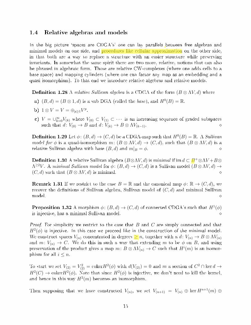
In the big picture `spaces are CDGA's' one can lay parallels between free algebras andminimal models on one side, and procedures like cellular approximation on the other side,in that both are a way to replace a structure with an easier structure while preservinginvariants. In somewhat the same spirit there are two more, relative, notions that can alsobe phrased in algebraic form. Those are relative CW-complexes (where one adds cells to abase space) and mapping cylinders (where one can factor any map as an embedding and aquasi isomorphism). To that end we introduce relative algebras and relative models.

Denition 1.28 A relative Sullivan algebra is a CDGA of the form (B ⊗ ΛV, d) where

a) (B, d) = (B ⊗ 1, d) is a sub DGA (called the base), and H0(B) = R.

b) 1⊗ V = V = ⊕p≥1Vp.

c) V = ∪∞k=0V(k) where V(0) ⊂ V(1) ⊂ · · · is an increasing sequence of graded subspacessuch that d : V(0) → B and d : V(k) → B ⊗ ΛV(k−1).

Denition 1.29 Let φ : (B, d)→ (C, d) be a CDGA-map such thatH0(B) = R. A Sullivanmodel for φ is a quasi-isomorphism m : (B ⊗ ΛV, d) → (C, d), such that (B ⊗ ΛV, d) is arelative Sullivan algebra with base (B, d) and m|B = φ.

Denition 1.30 A relative Sullivan algebra (B⊗ΛV, d) is minimal if im d ⊂ B+⊗ΛV +B⊗Λ≥2V . A minimal Sullivan model for φ : (B, d)→ (C, d) is a Sullivan model (B⊗ΛV, d)→(C, d) such that (B ⊗ ΛV, d) is minimal.

Remark 1.31 If we restrict to the case B = R and the canonical map φ : R → (C, d), werecover the denitions of Sullivan algebra, Sullivan model of (C, d) and minimal Sullivanmodel.

Proposition 1.32 A morphism φ : (B, d)→ (C, d) of connected CDGA's such that H1(φ)is injective, has a minimal Sullivan model.

Proof. For simplicity we restrict to the case that B and C are simply connected and thatH2(φ) is injective. In this case we proceed like in the construction of the minimal model.We construct spaces V(n) concentrated in degrees ≥ n, together with a d : V(n) → B ⊗ ΛV(n)

and m : V(n) → C. We do this in such a way that extending m to be φ on B, and usingpreservation of the product gives a map m : B ⊗ ΛV(n) → C such that H i(m) is an isomor-phism for all i ≤ n.

To start we set V(2) = V 2(2) = cokerH2(φ) with d(V(2)) = 0 and m a section of C2 ∩ ker d →

H2(C) → cokerH2(φ). Note that since H2(φ) is injective, we don't need to kill the kernel,and hence in this way H2(m) becomes an isomorphism.

Then supposing that we have constructed V(n), we set V(n+1) = V(n) ⊕ kerHn+1(m) ⊕

15

cokerHn+1(m) with the kernel in degree n and the cokernel in degree n+ 1. We set d on thecorkernel 0 and m on the cokernel a section of Cn+1 ∩ ker d → Hn+1(C) → cokerHn+1(m).Further d on kerHn+1(M) should map in B ⊗ ΛV(n) such that dw represents w, and at lastm on the added kernel should be such that m(dw) = dC(m(w)). That we can arrange d andm on kerHn+1(M) such that this holds follows in the same way as in the construction of theminimal model.

To then show that we get a minimal Sullivan model is similar to the end of the constructionof the minimal model.

1.5 Formal algebras

Up to this point for all algebras we have encountered, the minimal model of the algebra andthe minimal model of the cohomology are the same. This is of course no coincidence sinceup to this point all algebras were quasi-isomorphic to their cohomology. One can wonderwhether this always happens. Unfortunately it doesn't, as we see in the next example.

Example 1.33 The Heisenberg group H is the Lie group consisting of 3 × 3-matrices ofthe form 1 a b

0 1 c0 0 1

(a, b, c ∈ R)

We note that the inverse of such a matrix is given by1 a b0 1 c0 0 1

−1

=

1 −a ab− c0 1 −b0 0 1

From this it follows that the matrices with integer coecients form a closed subgroup HZ.

Consider the following minimal algebra

A = 〈x, y, z||x| = |y| = |z| = 1, dx = dy = 0, dz = xy〉

This is the minimal model of the deRham-complex of the quotient H/HZ. As a vector spaceit is spanned by x, y, z, xy, xz, yz and xyz. It follows that all spanning vectors are closed,except for z for which dz = xy. So we get that:

H(A) = spanR([x], [y], [xz], [yz], [xyz])

If we name [x] = α, [y] = β, [xz] = γ and [yz] = δ, we get the following generator-relation-description of H(A):

H(A) = 〈α, β, γ, δ|αδ + βγ = αβ = αγ = βδ = γ2 = δ2 = γδ = 0〉

16

Following the construction we described in the proof of Theorem 1.17 for making the min-imal modelM of H(A), we set:

M(1) = 〈v1, v2||v1| = |v2| = 1, dv1 = dv2 = 0〉

where v1 is to represent α and v2 is to represent β. Then for the next step we get a closedv1v2 we want to be exact. On the other hand we also need a representative for the closedelements γ and δ in degree 2. So we get:

M(2) = 〈v1, v2, w1, v3, v4||v1| = |v2| = |w1| = 1, |v3| = |v4| = 2, dvi = 0, dw1 = v1v2〉

Where v1, v2, v3 and v4 represent α, β, γ and δ respectively. Since from this point on theminimal model will only grow we see that H(A) has a much bigger minimal model than A.So we see that there is an algebra which is not quasi-isomorphic to its cohomology.

Remark 1.34 One can construct a similar example for a simply connected algebra, byputting x and y in degree 3 and z in degree 5, as we will encounter in Example 4.19.

In the context of Theorem 1.19 this makes life a little bit harder, since we really need to usethe whole algebra, we cannot get away with using just the cohomology. On the other handwe saw that there are a few examples of algebras where we can get away with doing this, soit is natural to give this class of algebras a special name:

Denition 1.35 A weak equivalence between CDGA's (A, d) and (B, d′) is a zigzag of quasi-

isomorphisms (A, d)'−→ (C1, d1)

'←− · · · '−→ (Cn, dn)'←− (B, d′). If such a weak equivalence

exists we call (A, d) and (B, d′) weakly equivalent.A CDGA (A, d) is called formal if it is weakly equivalent to a CDGA (H, 0) with trivialdierential. A manifold M is called formal is Ω(M) is a formal CDGA.

Remark 1.36 Of course, if (A, d) is weakly equivalent to some (H, 0), it is weakly equivalentto (H(A, d), 0) Furthermore, a weak equivalence can always be represented by a zigzagcontaining one algebra in between, namely the minimal model which A and B share.However, it is more natural to come across zig-zags which are longer than two maps, orzig-zags that do not end at H(A, d) but at some other algebra with zero dierential.

Example 1.37 By Example 1.7, all the spheres are formal manifolds. Exhibiting a mapφ : H(CP n)→ Ω(CP n) which sends [ω] to ω (for a xed symplectic form ω) one also ndsthat CP n is formal.

As Theorem 1.17 implies that quasi-isomorphic algebras have isomorphic minimal models(indeed having the same minimal models is equivalent to being weakly equivalent), we getthat:

Proposition 1.38 Let A be a formal CDGA, and let φ : M → A and φ′ : M ′ → H(A) be

minimal models of A and H(A) respectively, then there is an isomorphism ψ : M∼=−→M ′.

Combining this with Theorem 1.19 we get that:

17

Corollary 1.39 Let M be a formal and simply connected manifold. Then the rank ofπi(M) ⊗ Q as a Q-vector space equals the number of generator of the minimal model ofH(M) in degree i.

In particular, we see that for formal manifolds, the torsion free part of the homotopy can befully determined from the cohomology algebra.

1.6 Characterizing formality

The previous corollary justies why one is interested in nding formal manifolds among allmanifolds. Since the credo is `spaces are CDGA's', this means that we want to characterizeformal CDGA's among all CDGA's. In this section we discuss a few ways to characterizeformality of CDGA's.

We introduce the rst result by proving that low-dimensional manifolds are formal. Sincethe reason for this is algebraic in nature, namely Poincaré duality, we generalize this notionto general algebras.

Denition 1.40 A CGA H is called a Poincaré duality algebra (PDA) of dimension n ifH>n = 0, Hn = R · ω for some ω ∈ Hn and the multiplication induces perfect pairingsHn−i ⊗H i → Hn ∼= R for 0 ≤ i ≤ n.

Example 1.41 For any compact oriented manifoldM , its cohomology H(M) is a Poincaréduality algebra (this is what is commonly referred to as the Poincaré duality theorem).

Theorem 1.42 (Miller) Let A be a connected CDGA such thatH(A) is a Poincaré dualityalgebra of dimension D with H i(A) = 0 for 1 ≤ i ≤ k. If D ≤ 4k + 2, then A is formal.

Proof. Let φ : ΛV → A be the minimal model of A. We strive to nd a quasi isomorphismψ : ΛV → H(A). To that end we split V = C ⊕ N where d(C) = 0 and d : N → ΛVis injective. In the general construction of Theorem 1.17 C corresponds to the generatorsadded to create cohomology, while N corresponds to the generators that kill cohomology.

The most obvious way to make ψ as a quasi-isomorphism is setting ψ|ker d = [φ(−)], and thenwe better set ψ(N) = 0 to not spoil it being a quasi-iso. Then we want to extend ψ multi-plicatively, but for that to be well-dened we better have ψ(ker(d)∩(N ·ΛV )) = 0. Since φ is aquasi-isomorphism we conclude that we want to prove that every element x ∈ N ·ΛV ∩ker(d)is exact.

So we inspect C and N . Since H i(A) = 0 for 1 ≤ i ≤ k, we have that C = ⊕i≥k+1Ci.

Then the rst possible unwanted product lives in degree 2k + 2, so we have N = ⊕i≥2k+1Ni

and hence N · ΛV lives in degree 3k + 2 upwards. Consider now a homogeneous elementx ∈ N · ΛV such that dx = 0. If |x| 6= D we have that H |x|(ΛV ) ∼= H |x|(A) = 0 since3k + 2 ≥ D − k, and we conclude that x is exact. If |x| = D we note that this implies that

18

the lowest degree of C is within the range k+ 1 up to D−k−1 and in particular within thisrange there is non-zero cohomology, say Hj(ΛV ) ∼= Hj(A) 6= 0. The fact that the productHj(A) ⊗HD−j(A) → Hd(A) is a perfect pairing, means that in this case it is in particularsurjective. We conclude that the (up to exact elements) unique element v ∈ ΛV such that[φ(v)] = ω lives in ΛC.

So if x is not exact, it has to be (up to a scalar) a representative for ω, and hence x ∈ΛC + d(ΛV ) ⊂ ΛC +N · ΛV . Since N · ΛV ∩ ΛC = 0, we conclude that the representativefor ω that lives in ΛC has to be zero, which is a contradiction. So if x ∈ (N ·ΛV )D is closed,it represents 0 in cohomology, hence it is exact.

We see that every closed element of N · ΛV is exact, and hence ψ as described denes awell-dened quasi isomorphism ΛV → H(A), and hence A is formal.

The topological counterpart to this algebraic statement shows that low-dimensional mani-folds are formal, philosophically because `it is possible to choose representatives in a well-dened way, since there aren't so many choices to make'.

Corollary 1.43 LetM be a k-connected compact manifold for k ≥ 1. If dim(M) ≤ 4k+2,then M is formal.

Proof. If M is k-connected, then by denition πi(M) = 0 for 1 ≤ i ≤ k, so by Hurewicz weconclude that H i(M) = 0 for 1 ≤ i ≤ k. Since π1(M) = 0 we conclude that M is orientableand hence satises Poincaré duality, i.e. H(M) is a PDA of the same dimension as M . Theresult now follows immediately from the previous theorem.

In particular we see that simply connected manifolds up to dimension 6 are formal, so thetheory will start to get interesting from dimension 7 onwards (this will become apparantwhen we will discuss special holonomy in Section 3).

The proof of Theorem 1.42 also exposes a characterization of formality which on the onehand enables us to make ecient statements on formality of algebras constructed out ofothers, and on the other hand turns out be generalizable to such a degree that deciding onthe formality of manifolds will be a signicantly less complicated endeavour than it looks atrst glance.

Theorem 1.44 Let A be a CDGA. Then A is formal if and only if it has a minimal modelφ : ΛV → A such that V splits as V = C ⊕ N with d(C) = 0 and d : N → ΛV injectivewith the property that any closed element in N · ΛV is exact.

Proof. As seen in the proof of Theorem 1.42 given this data we can construct ψ : ΛV → H(A)dened by ψ|ker d = [φ(−)] and ψ|N = 0.

Now for the converse, we will show that the minimal model of a CDGA H with d = 0as constructed in Theorem 1.17 satises this property. Since A is assumed to be formal, the

19

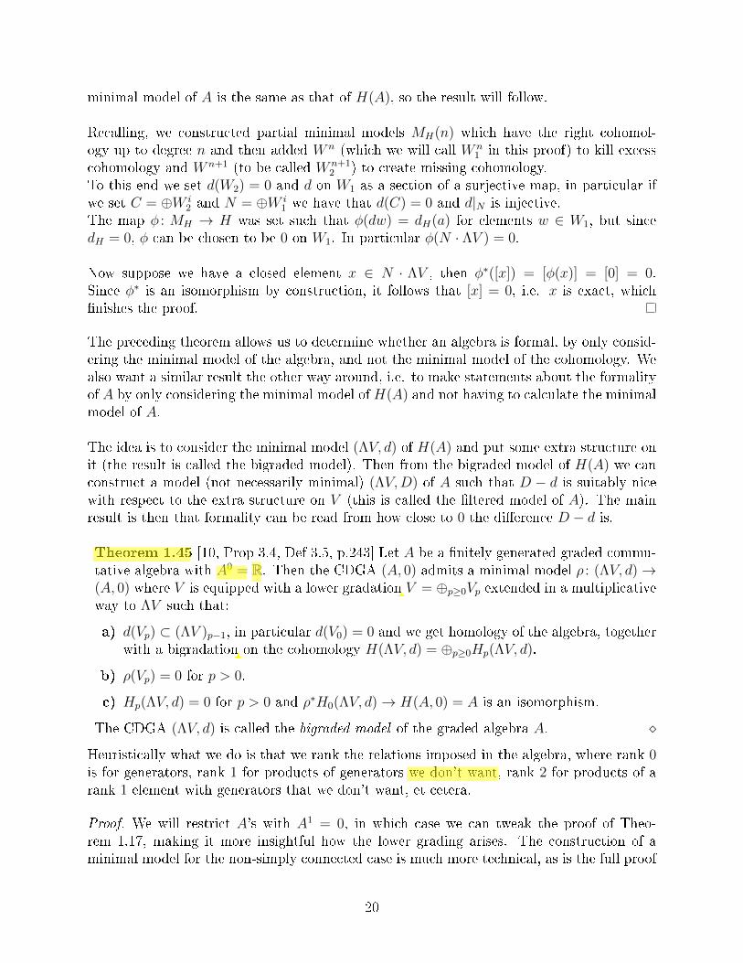
minimal model of A is the same as that of H(A), so the result will follow.

Recalling, we constructed partial minimal models MH(n) which have the right cohomol-ogy up to degree n and then added W n (which we will call W n

1 in this proof) to kill excesscohomology and W n+1 (to be called W n+1

2 ) to create missing cohomology.To this end we set d(W2) = 0 and d on W1 as a section of a surjective map, in particular ifwe set C = ⊕W i

2 and N = ⊕W i1 we have that d(C) = 0 and d|N is injective.

The map φ : MH → H was set such that φ(dw) = dH(a) for elements w ∈ W1, but sincedH = 0, φ can be chosen to be 0 on W1. In particular φ(N · ΛV ) = 0.

Now suppose we have a closed element x ∈ N · ΛV , then φ∗([x]) = [φ(x)] = [0] = 0.Since φ∗ is an isomorphism by construction, it follows that [x] = 0, i.e. x is exact, whichnishes the proof.

The preceding theorem allows us to determine whether an algebra is formal, by only consid-ering the minimal model of the algebra, and not the minimal model of the cohomology. Wealso want a similar result the other way around, i.e. to make statements about the formalityof A by only considering the minimal model of H(A) and not having to calculate the minimalmodel of A.

The idea is to consider the minimal model (ΛV, d) of H(A) and put some extra structure onit (the result is called the bigraded model). Then from the bigraded model of H(A) we canconstruct a model (not necessarily minimal) (ΛV,D) of A such that D − d is suitably nicewith respect to the extra structure on V (this is called the ltered model of A). The mainresult is then that formality can be read from how close to 0 the dierence D − d is.

Theorem 1.45 [10, Prop 3.4, Def 3.5, p.243] Let A be a nitely generated graded commu-tative algebra with A0 = R. Then the CDGA (A, 0) admits a minimal model ρ : (ΛV, d)→(A, 0) where V is equipped with a lower gradation V = ⊕p≥0Vp extended in a multiplicativeway to ΛV such that:

a) d(Vp) ⊂ (ΛV )p−1, in particular d(V0) = 0 and we get homology of the algebra, togetherwith a bigradation on the cohomology H(ΛV, d) = ⊕p≥0Hp(ΛV, d).

b) ρ(Vp) = 0 for p > 0.

c) Hp(ΛV, d) = 0 for p > 0 and ρ∗H0(ΛV, d)→ H(A, 0) = A is an isomorphism.

The CDGA (ΛV, d) is called the bigraded model of the graded algebra A.

Heuristically what we do is that we rank the relations imposed in the algebra, where rank 0is for generators, rank 1 for products of generators we don't want, rank 2 for products of arank 1 element with generators that we don't want, et cetera.

Proof. We will restrict A's with A1 = 0, in which case we can tweak the proof of Theo-rem 1.17, making it more insightful how the lower grading arises. The construction of aminimal model for the non-simply connected case is much more technical, as is the full proof

20

of this theorem, which can be found in the original paper.

When we look back at the proof of Theorem 1.17, basically the only thing we have todo is x the lower grading on W during the induction step, and x some sections. Fornotational purposes we dene W ′′ for the closed part of W (i.e. the cokernel we add) andW ′ for the non-closed part of W (i.e. the kernel we add with a shift in degree). Since lowergrading 0 is reserved for elements generating cohomology, we set W ′′ = W ′′

0 . Furthermore,since by assumption we already have a lower grading on ΛV we can nd a ltration on W ′,induced by d′, namely W ′

(p+1) = d′−1(ΛV )≤p. Then, if we nd a complementary basis of W ′(p)

in W ′(p+1) we set W ′

p+1 to be the span of this complement, so that W ′(p+1) = W ′

p+1 ⊕W ′(p),

we nd the lower grading of W ′ (note that this start iterating at 1). Also note that theconstruction with complimentary bases ensures that d(W ′

p) ⊂ (ΛW )p−1. Furthermore wecan look at the denition of ρ′ and see that for it we nd an a so that ρ(d′w′) = dAa. But,since dA = 0, we can always choose a = 0, and hence ρ′ = 0.

In this way we get lower grading 0 for creating cohomology, while lower degree p kills ofredundant cohomology in degree p + 1. Using that as philosophical inspiration, a carefulconsideration shows that with this construction we indeed get that Hp(ΛV, d) = 0 for p ≥ 1and that ρ∗|H0 is an iso. Since by construction ρ′ = 0, we see that ρ(Vp) = 0 for p ≥ 1 andsimilarly by construction d(Vp) ⊂ (ΛV )p−1, which nishes the proof.

Of course one should think ofA as the cohomology of some CDGA, and given a CDGA (A, dA)the bigraded model of the cohomology algebra H(A, dA) gives a model (not necessarilyminimal) of A, with only a slight tweak of the dierential.

Theorem 1.46 [10, Thm 4.4, Lem 4.5, Def 4.11, pp.248-252] Let (A, dA) be a connectedCDGA of nite type. Let ρ : (ΛV, d)→ (H(A, dA), 0) be a bigraded model of A. Then thereexists a dierential D on ΛV and a map π : (ΛV,D)→ (A, dA) such that:

a) D− d decreases the lower degree by at least two: D− d : Vp → (ΛV )≤p−2. That is, wecan write D = d + d2 + d3 + · · · where di is homogeneous of degree −i in the lowerdegree: di : Vp → (ΛV )p−i. In particular we have D = 0 on ΛV0.

b) [πv] = ρv for all v ∈ ΛV0.

c) π is a quasi-isomorphism.

We will call π : (ΛV,D)→ (A, dA) a ltered model of A with respect to ρ.

Proof. We x a linear map η : H(A) → ΛV0 such that ρη = id (which exists since ρ is asurjective linear map). We construct D and π inductively on V0, V1, ..., starting with basecases V0, V1 and V2.

First of all, by degree reasons, we need to set D = 0 on V0. Then set π on V0 suchthat dA(π(v)) = 0 and [π(v)] = ρ(v) for all v ∈ V0, and extend π to a homomorphismπ : (ΛV0, D)→ (A, dA). In particular [π(v)] = ρ(v) for all v ∈ ΛV0.Also for degree reasons we set D = d on V1, and since [πDv] = [πdv] = ρdv = 0 for v ∈ V1

21

we can extend π to a degree zero linear map π : V1 → A such that dAπz = πdz.Next suppose that v ∈ V2, then Ddv = d2v = 0 since dv ∈ Λ(V≤1) and the previous, andso dAπdv = 0, and we extend D to V2 by Dz = dz − η([πdz]). Taking all this together weextend D to a derivation on Λ(V≤2). Since for v ∈ V2 we have D2z = dDz = 0, we haveD2 = 0 on Λ(V≤2). Now since η maps into ΛV0 we have [πηα] = ρηα = α for all α ∈ H(A).In particular we get [πDv] = [πdv]− [πη[πdv]] = [πdv]− [πdv] = 0 for v ∈ V2, and so we canextend π to a degree zero linear map V2 → A such that dAπv = πDv, and we extend againto a homomorphism π : (Λ(V≤2), D)→ (A, dA).

For what comes we need the following claim, on describing D-closed elements as the sum ofD-exact elements and induced elements from η:

Claim: Let ρ : (ΛV, d) → (H, 0) be the bigraded model for a connected CGA H, andlet η : H → ΛV0 be a linear map such that ρη = id. Suppose (Λ(V≤n), D) is a CDGA suchthat (D − d) : Vl → (ΛV )≤l−2 for 0 ≤ l ≤ n. Assume u ∈ (ΛV )≤n−1 is D-closed. Then forsome v ∈ (ΛV )≤n and some α ∈ H it holds that: u = D(v) + η(α).

Proof of the Claim: Let n = 1, and u ∈ ΛV0. Then write u = dv + η(α) which can bedone since ρ∗ is an isomorphism, so choose α = ρ(u) and then [η(α) − u] = 0. But thendv = Dv so we're done.Next suppose that the claim holds for n − 1 and let u ∈ (ΛV )≤n−1 be D-closed. Writeu =

∑n−1j=0 uj, uj ∈ (ΛV )j. Then since Du = 0, by assumption on the relation between

D and d we have du ∈ (ΛV )≤n−3 and hence dun−1 = 0. Using that the bigraded modelhas trivial homology in higher degree we get un−1 = dvn for some vn ∈ (ΛV )n, but thenu−Dvn ∈ (ΛV )≤n−2 satises the hypothesis for n− 1, and hence u−Dvn = Dv′+ η(α) andthe result follows for v′ − vn.

Now suppose that D and π have been dened on ΛV(n) and let v ∈ Vn+1. Then by theclaim there are w ∈ (ΛV )≤n−1 (which may be chosen depending on v in a linear way) andα ∈ H(A) such that D(dv) = Dw + η(α). Applying π and using that [πηα] = α we getα = [πηα] = [dAπdv]− [dAπw] = 0 and hence D(dv − w) = 0.We extend D to Vn+1 by Dv = dv − w − η[π(dz − w)]. Then [πDv] = 0 and hence we canextend π to a homomorphism π : (Λ(V≤n+1), D)→ (A, dA).

Then by construction we have that D − d is a pertubation of degree 2, and by construc-tion (ΛV,D) is a Sullivan algebra, so we only have to show that π∗ is an isomorphism.From the Claim it follows that η∗ : H(A, dA) → H(ΛV,D) is surjective. Indeed if we takeu ∈ ΛV to be D-closed, then by the claim we nd v ∈ ΛV and α ∈ H(A, dA) such thatu = Dv+η(α) and then [u] = [η(α)] = η∗(α). Furthermore since [πv] = ρ(v) and ρη = id wehave π∗η∗ = id, so η∗ must be injective, hence an isomorphism. Then π∗, being the inverseis also an isomorphism.

Remark 1.47 We will not explicitely need it in what follows, but the bigraded model andltered model are essentially unique up to isomorphism.

22

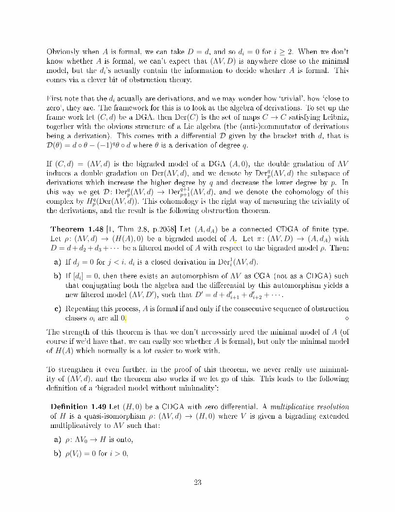
Obviously when A is formal, we can take D = d, and so di = 0 for i ≥ 2. When we don'tknow whether A is formal, we can't expect that (ΛV,D) is anywhere close to the minimalmodel, but the di's actually contain the information to decide whether A is formal. Thiscomes via a clever bit of obstruction theory.

First note that the di actually are derivations, and we may wonder how `trivial', how `close tozero', they are. The framework for this is to look at the algebra of derivations. To set up theframe work let (C, d) be a DGA, then Der(C) is the set of maps C → C satisfying Leibniz,together with the obvious structure of a Lie algebra (the (anti-)commutator of derivationsbeing a derivation). This comes with a dierential D given by the bracket with d, that isD(θ) = d θ − (−1)qθ d where θ is a derivation of degree q.

If (C, d) = (ΛV, d) is the bigraded model of a DGA (A, 0), the double gradation of ΛVinduces a double gradation on Der(ΛV, d), and we denote by Derqp(ΛV, d) the subspace ofderivations which increase the higher degree by q and decrease the lower degree by p. Inthis way we get D : Derqp(ΛV, d) → Derq+1

p+1(ΛV, d), and we denote the cohomology of thiscomplex by Hq

p(Der(ΛV, d)). This cohomology is the right way of measuring the triviality ofthe derivations, and the result is the following obstruction theorem.

Theorem 1.48 [1, Thm 2.8, p.2058] Let (A, dA) be a connected CDGA of nite type.Let ρ : (ΛV, d) → (H(A), 0) be a bigraded model of A. Let π : (ΛV,D) → (A, dA) withD = d+ d2 + d3 + · · · be a ltered model of A with respect to the bigraded model ρ. Then:

a) If dj = 0 for j < i, di is a closed derivation in Der1i (ΛV, d).

b) If [di] = 0, then there exists an automorphism of ΛV as CGA (not as a CDGA) suchthat conjugating both the algebra and the dierential by this automorphism yields anew ltered model (ΛV,D′), such that D′ = d+ d′i+1 + d′i+2 + · · · .

c) Repeating this process, A is formal if and only if the consecutive sequence of obstructionclasses oi are all 0.

The strength of this theorem is that we don't necessairly need the minimal model of A (ofcourse if we'd have that, we can easily see whether A is formal), but only the minimal modelof H(A) which normally is a lot easier to work with.

To strengthen it even further, in the proof of this theorem, we never really use minimal-ity of (ΛV, d), and the theorem also works if we let go of this. This leads to the followingdenition of a `bigraded model without minimality':

Denition 1.49 Let (H, 0) be a CDGA with zero dierential. A multiplicative resolutionof H is a quasi-isomorphism ρ : (ΛV, d) → (H, 0) where V is given a bigrading extendedmultiplicatively to ΛV such that:

a) ρ : ΛV0 → H is onto,

b) ρ(Vi) = 0 for i > 0,

23

c) Hi(ΛV, d) = 0 for i > 0 and H0(ρ) : H0(ΛV, d)→ H is an isomorphism.

Then in the same way as we can talk about a ltered model with respect to a bigradedmodel, we can also talk about a ltered model with respect to a multiplicative resolution(the denition copies literally here since it does not make reference to minimality of (ΛV, d)).We do not care for existence of a ltered model with respect to any multiplicative resolutionfor the moment, but the immediate generelization of Theorem 1.48 is as follows:

Corollary 1.50 [1, Cor 2.9, p.2058] Let (A, dA) be a connected CDGA. Let φ : (ΛV, d)→(H(A), 0) be a multiplicative resolution of A. Let π : (ΛV,D)→ (A, dA) with D = d+ d2 +d3 + · · · be a ltered model of (A, dA) with respect to the multiplicative resolution φ. Ifdj = 0 for j < i, then di is a closed derivation in Der1

i (ΛV, d) and we denote its cohomologyclass by oi. Then (A, dA) is formal if and only if oi = 0 for all i.

Proof of Theorem 1.48. .a) If D = d + di + di+1 + · · · the equation D2 = 0 yields d2 + ddi + did + O(i + 2) = 0where by O(i + 2) we mean terms decreasing the lower degree by at least i + 2 and henceddi + did = D(di) = 0.b) Suppose that we are in the case D = d + di + di+1 + · · · with [di] = 0. That meansthat there is an element φi ∈ Der0

i−1(ΛV, d) such that di = dφi − φid. We consider the mape−φi : ΛV → ΛV . Here we dene the exponential by the usual formula

e−φi = id− φi +φ2i

2− φ3

i

6+ ...

Since φi decreases the lower degree by i − 1 and every homogeneous element of ΛV has anite lower degree, we conclude that this is well-dened. Furthermore by the usual argu-ments we have that e−φi is a morphism of CGA's with inverse eφi . If we set D′ = eφiDe−φi

then obviously the map e−φi becomes an isomorphism (ΛV,D′)→ (ΛV,D).

The important calculation is now:

D′ = (id + φi +O(i+ 1))(d+ di +O(i+ 1))(id− φi +O(i+ 1))

= d+ (φid− dφi + di) +O(i+ 1)

Then since by denition di = dφi − φid we conclude that D′ = d + O(i + 1), i.e. D′ =d+ d′i+1 + d′i+2 + · · · .c) If A is formal then by the discussion above the question is academical, so we show thatif the sequence of obstructions vanishes the algebra is formal.

Note we have a zigzag of (quasi-)isomorphisms starting (A, dA)π←− (ΛV,D2)

e−φ2←−−− (ΛV,D3) · · · .Then since the e−φr − id decreases the lower degree by at least r − 1 we have that forany element, the pertubations of e−φr have to vanish at some point, i.e. Φ: = · · · e−φr e−φr−1 · · · e−φ2 is a well-dened isomorphism of CGA's and since Dr − d decreases the lowerdegree by at least r it follows that it is an isomorphism of CDGA's from (ΛV, d)→ (ΛV,D).

24

So we see that we have a zigzag of (quasi-)isomorphisms (A, dA)π←− (ΛV,D)

Φ←− (ΛV, d)ρ−→

(H(A), 0) and we conclude that A is formal.

Proof of Corollary 1.50. We didn't use minimality of ρ : (ΛV, d)ρ−→ (H(A), 0) to construct

the zig-zag of (quasi)-isomorphisms (A, dA)π←− (ΛV,D)

Φ←− (ΛV, d)ρ−→ (H(A), 0) in the previ-

ous proof, so it still applies when ρ is just a multiplicative resolution.

We conclude that since (A, dA) is still weakly equivalent to (H(A), 0) it is still formal underthis weakened assumption.

25

2 Rational homotopy theory and CDGA's

In what we have discussed the main philosophical point is the assignment

manifolds → minimal CDGA's over R

via the minimal model of the deRham complex. This assignment is not at all surjective (forinstance in the simply connected case we need to have Poincaré duality which need not occurin a minimal CDGA), but when we broaden our viewpoint to topological spaces we will ndan equivalence of categories between the (naive) homotopy categories of rational homotopytypes and the category of isomorphism classes of minimal CDGA's (at least if we imposethings like nite type and simply connectedness on both sides).In particular we will construct a functor from topological spaces to CDGA's over Q, calledAPL, which will have the property that H(APL(X)) ' H(X;Q) and then we associate to arational homotopy type [X] the minimal model of APL(X) (note that a rational homotopyequivalence induces isomorphisms on H(−;Q) and hence quasi-isomorphisms on APL, so ra-tional equivalent spaces have the same minimal model.). On the other hand, we will buildfrom a minimal algebra a space whose minimal model is the one we started with.

We will show that for manifolds the real and rational theories are equivalent, in that theminimal model dened via APL is up to extending scalars isomorphic to each other, and alsothat the notion of formality are equivalent. In fact, we will show that for a manifold X,APL(X) and Ω∗(X) are weakly equivalent in a suitable sense. All this will be done closelyfollowing the book by Félix, Halperin and Thomas [7].

In what follows we will consider a CDGA to be dened over a eld K of characteristic0. Note that the denition of a CDGA as given before does not makes extrinsic reference tothe eld R and hence we can safely replace it any other eld.

2.1 Simplicial objects and APL

Denition 2.1 The simplex category ∆ is dened to have objects [n] = 0, ..., n for everynatural n ≥ 0 together with morphisms which are order preserving maps (nb: not strictlyorder preserving).

Denition 2.2 For a category C, a simplicial object in C is a contravariant functor ∆op → C.A morphism of simplicial objects is a natural transformation between the two functors. Wewill denote the category of simplicial objects in C by sC.

We note that there are two important families of morphisms in the simplex category, namelythe maps δi : [n− 1] → [n] which are the injections that does not hit the number i and themaps σi : [n + 1] → [n] which are surjections that hit i twice. These satisfy the following

26

relations:δjδi = δiδj−1 if i < jσjσi = σiσj+1 if i ≤ j

σjδi =

δiσi−1

idδi−1σj

ififif

i < ji = j, j + 1i > j + 1

Since all these maps together generate the morphisms in the simplex category we concludethe following.

Lemma 2.3 A simplicial object in C is the same as a sequence of objects Knn≥0 in Ctogether with morphisms ∂i : Kn+1 → Kn (called the face maps) for 0 ≤ i ≤ n + 1 andsj : Kn → Kn+1 (called the degeneracy maps) for 0 ≤ j ≤ n satisfying the identities

∂i∂j = ∂j−1∂i if i < jsisj = sj+1si if i ≤ j

∂isj =

si−1∂iid

sj∂i−1

ififif

i < ji = j, j + 1i > j + 1

Furthermore a morphism between simplicial objects f : L → K is the same as a sequenceof morphisms fn : Ln → Kn that commute with the face and degeneracy maps.

Example 2.4 The most used example of simplicial object is the simplicial set of singularchains S(X) of a topological space X. Here we set S(X)n = σ : ∆n → X|σ continuous.As face and degenaracy maps we set ∂i(σ) = σλi and sj(σ) = σρj where λi : ∆n → ∆n+1

sends (x0, ..., xn) to (x0, ..., 0, ..., xn) with the 0 inserted in the i'th slot and ρj : ∆n → ∆n−1

sends (x0, ..., xn) to (x0, ..., xj + xj+1, ..., xn).

Furthermore a continuous map f : X → Y gives a map of simplicial sets, by sending σto f σ.

We now wish to construct CDGA's in a systematic manner from simplicial sets and simplicialCDGA's. For this consider K a simplicial set and A = Ann≥0 a simplicial CDGA. Notethat Apnn≥0 is a simplicial vector space and in particular a simplicial set for every p. Weconstruct a CDGA A(K) in the following manner:

We set Ap(K) to be the set of morphisms from K to Ap seen as simplicial sets. So anelement of Ap(K) is a map Φ that sends σ ∈ Kn to Φ(σ) ∈ Apn such that ∂iΦ = Φ∂i andsjΦ = Φsj.

Addition, scalar multiplication and dierential are given as one would expect by (Φ +Ψ)(σ) = Φ(σ) + Ψ(σ), (λΨ)(σ) = λ · (Ψ(σ)) and (dΨ)(σ) = d(Ψ(σ)). Similarly we mul-tiply (Φ ·Ψ)(σ) = Φ(σ) ·Ψ(σ). That we get a CDGA in this way is more or less immediate,and one argues similary to showing that Set(S,G) inherits a group structure if G is a group.

If φ : K → L is a morphism of simplicial sets, we set a morphism A(φ) : A(L) → A(K)

27

by A(φ)(Φ)(σ) = Φ(φ(σ)). If θ : A→ B is a morphism of simplicial CDGA's, then we get amorphism θ(K) : A(K)→ B(K) where (θ(K)Φ)(σ) = θ(Φ(σ)). In this way we get a functorsSetop × scdga→ cdga.

If X is a topological space and A is a simplicial CDGA, we write A(X) for A(S(X)), andhence a simplicial CDGA gives a contravariant functor Top→ cdga.

Now the idea is that given a simplex ∆n → X we can make sense of a `polynomial formon X' if it formally pulls back to a polynomial dierential form on ∆n and this is preciselywhat is at the core of the abstract general construction outlined above. To dene APL(X)we need to dene the simplicial CDGA APL.

Denition 2.5 We set (APL)n to be the CDGA generated by elements t0, ..., tn, dt0, ..., dtnwith |ti| = 0, |dti| = 1, subject to the relations

∑ti = 1 and

∑dti = 0. We set the face

and degeneracy maps dened by

∂i(tk) =

tk if k < i0 if k = itk−1 if k > i

sj(tk) =

tk if k < j

tk + tk+1 if k = jtk+1 if k > j

If K ⊂ R, the CDGA (APL)n is the subalgebra of Ω∗(∆n) consisting of polynomial forms inthe coordinates ti with coecients in K, hence the name. In this setting we also recognize∂i as the pullback by λi and sj as the pullback by ρj.

Denition 2.6 We dene the polynomial dierential forms, APL(X) (sometimes denotedAPL(X,K) when we want to stress the eld), to be the CDGA obtained by the simplicialCDGA APL and the simplicial set S(X).

We see that a polynomial dierential p-form α ∈ ApPL(X) is an assignment to every contin-uous map σ : ∆n → X a polynomial p-form α(σ) ∈ (ApPL)n such that α(∂iσ) = ∂i(α(σ)) andα(sjσ) = sj(α(σ)).

The important property of APL is the following:

Theorem 2.7 [7, Cor 10.10, p.126] There is a natural weak equivalence between C∗(X;K)and APL(X;K). In particular there is a natural isomorphism H∗(X;K) ∼= H(APL(X;K)).

Rationale. We will not proof this, but what one should have in mind is that one can see apolynomial dierential p-form α as a morphism of the p-simplices of X to K by taking asimplex f : ∆p → X and then formally integrating α(f) over ∆p (note that integrating apolynomial over a simplex is a purely formal algebraic aair).

28

2.2 Comparing APL(M ;R) and Ω(M)

If M is a manifold, we now have constructed two model CDGA's (over R) for M , namelyAPL(M ;R) and Ω(M), and we set up an algebraic theory for Ω(M). If we want to extend thistheory to arbitrary topological spaces, we would better make sure that APL(M ;R) and Ω(M)are comparable. Since we're interested in minimal models, which measure weak isomorphismclasses, we will show that there is a natural weak equivalence between APL(M ;R) and Ω(M).

To do this we rst consider the simplicial set of smooth simplices S∞(M). As one wouldexpect we set S∞n (M) = σ : ∆n →M |σ smooth, together with face and degeneracy mapsprecomposition by the structure maps of the standard simplex. In this way S∞(M) is asimplicial subset of S(M).

Next we want to construct a simplicial CDGA to model the deRham-complex. As an elementAPL is an abstract entity that pullsback through each simplex to a polynomial form on thestandard simplex, we are inclined to dene the simplicial CDGA AdR by (AdR)k = Ω(∆k)with face and degenracy maps λ∗i and ρ

∗j .

We note that by the remark before, since any polynomial is in particular smooth we havea canonical inclusion of simplicial CDGA's APL(−;R) → AdR. This gives a natural mor-phism βM : APL(S∞(M);R) → AdR(S∞(M)). On the other hand the natural inclusionS∞(M)→ S(M) gives a natural morphism γM : APL(M ;R)→ APL(S∞(M);R).

At last consider an element of AdR(S∞(M)). This is a function Φ which assigns to ev-ery smooth simplex σ a smooth form Φ(σ) ∈ Ω(∆|σ|), which commutes with face anddegeneracy maps. If one considers some smooth form α ∈ Ω(M) we can construct anelement of AdR(S∞(M)) by Φα(σ) = σ∗(α). In particular we get a natural morphismαM : Ω(M)→ AdR(S∞(M)). So we are in the following situation:

Ω(M)αM−−→ AdR(S∞(M))

βM←−− APL(S∞(M);R)γM←−− APL(M ;R)

Theorem 2.8 [7, Thm 11.4,p.135] All three of αM , βM and γM are quasi-isomorphism andhence Ω(M) and APL(M ;R) are weakly equivalent.

An advantage of the somewhat abstract way to dening these CDGA's, is that we can veryeectively construct quasi-isomorphism. The idea is that, given two simplicial CDGA's, ifwe nd a morphism between them that induces a quasi isomorphism at every level, thenwe get a quasi-isomorphism when plugging in an arbitrary simplicial set in either simplicialCDGA. We do need a small technical property of simplicial objects

Denition 2.9 A simplicial object A in a concrete category C (i.e. a category where theobjects are sets with extra structure, think Set, Top, cdga) is called extendable if for anyn ≥ 1 and any I ⊂ 0, ..., n, given Φi ∈ An−1 for every i ∈ I such that ∂iΦj = ∂j−1Φi fori < j then there is an element Φ ∈ An such that Φi = ∂iΦ for every i ∈ I.

29

The important proposition is then:

Proposition 2.10 [7, Prop 10.5,p.119] Suppose θ : D → E is a morphism of simplicialCDGA's. Assume that θn : Dn → En is a quasi-isomorphism for all n ≥ 0 and that bothD and E are extendable. Then for any simplicial set K, θ(K) : D(K)→ E(K) is a quasi-isomorphism.

Then not surprising are the following lemmas:

Lemma 2.11 [7, Lem 10.7,p.123]

a) APL(−;K)0 = K · 1

b) H(APL(−;K)n) = K · 1 for n ≥ 0

c) Each ApPL is extendable.

Lemma 2.12 [7, Lem 11.3,p.134]

a) (AdR)0 = R

b) H((AdR)n) = R for n ≥ 0

c) Each ApdR is extendable.

This asserts that any comparison between AdR and APL needs only to be checked on standardsimplices. Then to compare Ω(M) and AdR(S∞(M)) and APL(S∞(M);R) and APL(M ;R)we really need to compare functors from n-dimensional manifolds to cochain algebras. Thekeywords here are, as always with manifolds: localizing and gluing, and the result is:

Lemma 2.13 [7, Lem 11.5, p.135] Let θ : A→ B be a natural transformation between twofunctors from n-dimensional manifolds to cochain algebras. Suppose that:

a) H(A(Rn)) = R = H(B(Rn))

b) If U and V are open in M and θU , θV and θU∩V are quasi-isomorphisms, then so isθU∪V

c) If O = tiOi is the disjoint union of open sets, then θO =∏

i θOi.

Then θM is a quasi-isomorphism for all smooth n-dimensional manifolds.

Proof. Consider a family of open subsets Vλ ⊂ M that is closed under nite intersection,and such that any open subset ofM is the union of some of the Vλ. Given such a family, it ispossible to write M = O ∪W where O = tiOi and W = tjWj are both disjoint unions outof elements of the given family. Suppose that θVλ is a quasi-isomorphism for any element ofthe family, then by induction of p so is θVλ1

t···tVλp and it follows that θO, θW and θO∩W arequasi-isomorphisms, and hence θM is as well.

Now consider U to be open in Rn and consider the family of open cubes in U , certainly afamily as described in the above. Then, by the rst assumption, the natural transformation

30

for any open cube is a quasi-isomorphism, and hence, by the above, θU is a quasi-isomorphism.

Since the family of open subsets of M dieomorphic to an open subset of Rn is a familyas described at the start, the two above parts show that θM is a quasi-isomorphism.

We are now ready to prove Theorem 2.8:

Sketch of proof of Theorem 2.8. To see that αM is a quasi-isomorphism, note thatH(Ω(Rn)) =R as is known, while one can show that H(AdR(S∞(Rn))) = H(C∗∞(Rn)) = R, where C∗∞are the smooth singular cochains, but we will not show this as then we'd have to go even astep deeper in the lingo of simplicial objects and functors.

Next note that for U, V ⊂M open we have a short exact sequence:

0→ Ω(U ∪ V )→ Ω(U)⊕ Ω(V )→ Ω(U ∩ V )→ 0

and similarly

0→ AdR(S∞(U) ∪ S∞(V ))→ AdR(S∞(U))⊕ AdR(S∞(V ))→ AdR(S∞(U ∩ V ))→ 0

where AdR(S∞(U)∪S∞(V )) is naturally quasi-isomorphic to AdR(S∞(U∪V )) by barycentricsubdivision. Then an argument with the long exact sequence shows that αU∪V is a quasi-isoif αU , αV and αU∩V are.Finally if O = tiOi then αO =

∏i αOi and hence by Lemma 2.13 αM is a quasi-isomorphism

for all M .

That βM is a quasi-isomorphism is a direct result of Lemma 2.11, Lemma 2.12 and Propo-sition 2.10.

Like before we only note (but not show) that APL(S∞(Rn);R) = R. To show that γU∪Vis a quasi isomorphism if γU , γV and γU∪V are, note that barycentric subdivision C∗(U) +

C∗(V )'−→ C∗(U ∪V ) restrict to smooth barycentric subdivision C∞∗ (U)+C∞∗ (V )

'−→ C∞∗ (U ∪V ). Then by an argument with the long exact sequence in homology we see that if C∞∗ (U)→C∗(U), C∞∗ (V )→ C∗(V ), C∞∗ (U ∩ V )→ C∗(U ∩ V ) are quasi-isos, then so is C∞∗ (U ∪ V )→C∗(U ∪ V ). Dually we see that if γU , γV and γU∩V are quasi-isomorphisms, then so is γU∪V .Clearly γtiOi =

∏i γOi and so by Lemma 2.13 γM is a quasi-iso for all M .

We can now enlarge our theory of formal manifolds to the theory of formal spaces, whichwill sometimes be handy when we want to use intermediate constructions which may not bemanifolds, for instance the wedge of two spaces.

Denition 2.14 A topological space X is called K-formal if APL(X;K) is a formal CDGAover K. If we do not specify the eld, i.e. if we say that X is formal, we will mean that itis Q-formal.

At this point we should notice the following:

31

Lemma 2.15 Let K be a eld of characteristic 0, and let (ΛV, d) → APL(X;Q) be aminimal model. Then by extending scalars from Q to K, we obtain a minimal model(ΛV ′, d′)→ APL(X;K) where V ′ = V ⊗Q K (and similarly for d′).

Since Theorem 1.44 also applies for elds other than R, we conclude:

Lemma 2.16 For a eld K of characteristic 0, a space X is K-formal if and only if it isQ-formal.

This remark, combined with Theorem 2.8 we conclude:

Proposition 2.17 A manifold M is formal in the sense of Denition 1.35 if and only if itis formal in the sense of Denition 2.14.

2.3 Minimal models and homotopy groups

As mentioned in the previous chapter, there is a connection between the minimal model ofΩ(M) and the rational homotopy groups (Theorem 1.19). In this section we will discuss theconstruction and proof, which is more topological in avour, using APL.

First we discuss a way to assigning to maps between topological spaces (or maps betweenalgebras), maps between the minimal models. Consider two CDGA's A and B with mini-mal models mX : ΛV → A and mY : ΛW → B and a map φ : A → B. The lifting lemma(Proposition 1.25) yields that there is an (up to homotopy unique) map mφ : ΛV → ΛWsuch that φ mX ' mY mφ. Furthermore the homotopy class of mφ depends only on thehomotopy class of φ. We call mφ a Sullivan representative of φ. Note that the linear partQ(mφ) : V → W is independent of the choice since homotopic morphisms have the samelinear part.

Going one step further, given a continuous map f : Y → X we can take a Sullivan represen-tative of APL(f) : APL(X;K) → APL(Y ;K), and take the linear part Q(f) : = Q(mAPL(f)).Suppose for instance that we have a map f : Sk → X. Then the kth part of Q(f) denes amap V k → K (where ΛV is the minimal model of X). Note that Q(f) only depends on thehomotopy class of f .

To make this precise, let X be a topological space and x a minimal model mX : ΛV →APL(X;K). Furthermore, denote minimal models of Sk by 〈e; |e| = k, de = 0〉 for k oddand 〈e, e′; |e| = k, de = 0, de′ = e2〉 for k even. Let α ∈ πk(X) be a homotopy element,represented by a : Sk → X. Then having xed the minimal model, Q(a) : V k → K · e onlydepends on α. In this way we get a pairing 〈−;−〉 : V × π∗(X)→ K by:

〈v;α〉e =

Q(a)(v) v ∈ V k

0 deg v 6= degα

The theorem by Sullivan is made precise as follows:

32

Theorem 2.18 [7, Thm 15.11, p.208] Suppose that Hi(X;K) is of nite type. Then themap νX : V → HomZ(π∗(X);K), v 7→ 〈v;−〉 is a linear isomorphism.

To make the statement even reasonable, we rst show that the pairing is bilinear:

Lemma 2.19 The pairing 〈−;−〉 is bilinear.

Proof. Linearity in V k is clear by denition (since Q(a) is linear), so we will focus on linearity(really addivity) in the second slot. So let α0 and α1 be two elements of πk(X) representedby maps a0 : Sk → X and a1 : Sk → X. If we denote by j the pinch map Sk → Sk ∨ Sk,then α0 + α1 is represented by the composite (a0, a1) j.

Denote by i0 and i1 the two obvious inclusions Sk → Sk ∨ Sk, then the canonical basisw0, w1 of Hk(Sk ∨ Sk;K) is determined by i∗j(wl) = 1 if j = l and 0 otherwise. It followsthat the minimal of Sk ∨ Sk is give by

m : (Λ(e0, e1, ...), d)→ APL(Sk ∨ Sk)

where e0 and e1 are cocycles of degree k, such that H(m)[ei] = wi, and where the othergenerators are in higher degree to kill of any excess products (we will come back to this in5.3).

A Sullivan representative φ0 for i0 needs to satisfy H(φ0)[e0] = [e] and H(φ0)[e1] = 0 bydenition of ei. Since there are no coboundaries in degree k on either side this means thatφ0e0 = e and φ0e1 = 0, and hence Q(i0)e0 = e and Q(i0)e1 = 0. Similarly Q(i1)e0 = 0,Q(i1)e1 = e and Q(j)e0 = e = Q(j)e1.

Now since (a0, a1) i0 = a0 and (a0, a1) i1 = a1 we see that Q(a0, a1)v = 〈v;α0〉e0 + 〈v;α1〉e1

and composing with Q(j) we conclude that Q(a)v = (〈v;α0〉 + 〈v;α1〉)e which is what wasto be shown.

Sketch of proof of Theorem 2.18. We x k ≥ 2 and denote r = r(X) the least integer suchthat πr(X)(X) 6= 0. To show that νkX : V k

X → HomZ(πk(X),K) is an isomorphism we will useinduction on k − r.If k = r we know that the Hurewicz homomorphism πr(X) → Hr(X;Z) is an isomorphismand furthermore that Hi(X;Z) = 0 for i < k. Also we see that H i(X;K) = 0 for i < kand Hr(X;K) ∼= Hom(Hr(X;Z),K). The former implies that V i = 0 for i < k and henceHr(mX) is an isomorphism V r → Hr(X;K).When we look at the denition of the Hurewicz homomorphism and of νrX we conclude thatunder these isomorphisms they coincide and hence νrX is an isomorphism.

If k > r, note that any space X is weakly equivalent to a CW complex Y via some mapf : Y → X. For this f the Sullivan representative is an isomorphism between the minimalmodels of X and Y . Since in particular Q(f) and π∗(f) are isomorphisms, by naturality wemay assume X to be an CW complex.

33

Next, let K be an Eilenberg-MacLane space of type (πr(X), r) together with a continu-ous map g : X → K such that πr(g) = id. By factoring g via a bration and a homotopyequivalence we may assume that there is a bration p : X → K such that πr(p) is an isomor-phism.Consider a typical ber F of p. By the long exact sequence of the bration we conclude thatπi(F ) = 0 for i ≤ r, and in partcular r(F ) ≥ r(X) + 1.

By looking at the structure of models of bases, total spaces and bers of brations (thenuances of which we will discuss in Section 4.2), although we will leave this as a completeblack box), we are able to identify νkX and νkF via isomorphisms between πk(X) and πk(F )and the k'th parts of the minimal models of X and F . Since r(F ) ≥ r(X) + 1, we havek− r(F ) < k− r(X) so by induction on this number we see that νkF is an isomorphism, andwe conclude that νkX is an isomorphism.

2.4 Spatial realization

We will end the part of topological constructions by showing that up to reasonable equiv-alence, the category of minimal models is the same as the category of topological spaces.This will turn out to be useful in what follows, since we can deduce pushout and pullbackproperties of squares of CDGA's out of those of squares of topological spaces. To not wit toomuch on the somewhat more diehard topology, we will only give a brief outline of chapter17 of Felix, Halperin and Thomas [7], which in its own right is partly based on May [18] andSullivan [22].

For what comes we will restrict ourselves to simply connected rational CDGA of nite type,so unless otherwise stated we will assume every algebra mentioned to have these properties.

The plan de campagne is as follows.We will construct a contravariant functor assigning to any algebra (A, d) a CW-complex |A, d|and to any map (A, d) → (B, d) of Sullivan algebras a continuous map |φ| : |B, d| → |A, d|,such that the functor will have the following properties:

First for any Sullivan algebra (ΛV, d) we get a quasi-isomorphism (ΛV, d)→ APL(|ΛV, d|).In particular if (ΛV, d) is minimal, it is the minimal model of its own spatial realization.

Next any morphism φ : (ΛV, d) → (ΛW,d) of Sullivan algebras is a Sullivan represen-tative of |φ| : |ΛW,d| → |ΛV, d| with respect to quasi-isomorphisms mentioned above.

Then two morphisms φ, ψ : (ΛV, d)→ (ΛW,d) between Sullivan algebras are homotopicif and only if |φ| and |ψ| are homotopic as continuous maps.

For any Sullivan representative φ : (ΛV, d) → (ΛW,d) of a continuous map f : X →Y between CW-complexes with rational cohomology of nite type, we nd mapshX : X → |ΛW,d| and hY : Y → |ΛV, d| such that |φ| hX ' hY f and hX andhY are rational homotopy equivalences.

34

Restricting to simply connected CW complexes with rational cohomology of nite type andsimply connected Sullivan algebras we will nd bijections:

rational homotopy

types

→

isomorphism classes of

minimal Sullivan algebrasover Q

homotopy classes ofcontinuous maps

between rational spaces

→

homotopy classes ofmorphisms of Sullivan algebras

over Q

We will describe the functor | · | as a composition of a contravariant functor 〈·〉 from CDGA'sto simplicial sets, and a covariant functor | · | from simplicial sets to CW-complexes. Mostof the time we can do all the constructions over any eld K, but in the end we are mostlyinterested in K = Q.

Denition 2.20 Let (A, d) be a CDGA, we construct the simplicial set 〈A, d〉 by setting

〈A, d〉n = σ : (A, d)→ (APL)n|σ is a map of CDGA's,

or in alternative notation cdga((A, d), (APL)n). We set face and generacy maps by ∂iσ =∂i σ and sjσ = sj σ.If φ : (A, d) → (B, d) is a morphism of CDGA's then 〈φ〉 : 〈B, d〉 → 〈A, d〉 is given by〈φ〉(σ) = σ φ.

Remark 2.21 If we recall that APL was a functor from simplicial sets to CDGA's set bysSet(K,APL) we get a natural bijection

cdga((A, d), APL(K))→ sSet(K, 〈A, d〉)

set by φ 7→ f with f(σ)(a) = φ(a)(σ). In particular APL(·) and 〈·〉 are adjoint functorsbetween CDGA's and simplicial sets. From this we get a canonical morphism ηA : (A, d)→APL〈A, d〉 adjoint to the identity of 〈A, d〉.

Then to dene the functor | · | from simplicial sets to CW-complexes recall the mapsλi : ∆n−1 → ∆n and ρj : ∆n+1 → ∆n where λi sends (x0, ..., xn) to (x0, ..., 0, ..., xn) withthe 0 inserted in the i'th slot and ρj sends (x0, ..., xn) to (x0, ..., xj + xj+1, ..., xn).

Denition 2.22 Let K be a simplicial set. Using Kn as a index set we dene |K| to be

|K| = (tnKn ×∆n)/ ∼

where we identify (∂iσ, x) ∼ (σ, λix) and (sjσ, x) ∼ (σ, ρjx).Given a map f : K → L of simplicial sets, written as f = fn : Kn → Ln, the mapsfn × id : Kn × ∆n → Ln × ∆n are continuous and preserve ∼, so they factor to a map|f | : |K| → |L| in a functorial way.

35

We also describe an adjoint pair in this case. In particular for a simplicial set K and aσ ∈ Kn, the inclusion σ × ∆n → tnKn × ∆n descends to a map qσ : ∆n → |K|, whichgives an inclusion of simplicial sets ξK : K → S(|K|), σ 7→ qσ.

On the other hand, given a topological spaceX we get a map tnSn(X)×∆n → X which sendsa pair (σ, y) to σ(y). This map factors through to the quotient into a map sX : |S(X)| → X.

These maps acts in some sense as inverses to each other:

Proposition 2.23 [7, Prop 17.3, p.242]

a) If X is a simply connected CW-complex, then sX is a homotopy equivalence.

b) If K is a simplicial set such that |K| is simply connected, then |ξK | is a homotopyequivalence.

Combining both functors we arrive at our spatial realization functor from CDGA's to CW-complexes:

Denition 2.24 Let (A, d) be a CDGA. We dene its spatial realization by |A, d| = |〈A, d〉|.Similarly, we dene the spatial realization of a map φ : (A, d)→ (B, d) by |φ| = |〈φ〉|.

We now give brief outlines of constructions used to prove the properties described at thestart, while referring to FHT [7] for the proofs.

First, we describe the quasi-isomorphism m(ΛV,d) : (ΛV, d)'−→ APL(|ΛV, d|). Note from be-

fore the inclusion ξ : = ξ〈ΛV,d〉 : 〈ΛV, d〉 → S(|ΛV, d|), one can show that applying APL to itgives rise to a surjective quasi-isomorphism APL(ξ) : APL(|ΛV, d|)→ APL(〈ΛV, d〉). Then wecan apply the lifting lemma (Lemma 1.22) to the canonical map η(ΛV,d) to obtain the mapm(ΛV,d) : (ΛV, d)→ APL(|ΛV, d|).

Theorem 2.25 [7, Thm 17.10.(ii), p.250] If K = Q, the mapm(ΛV,d) is a quasi-isomorphism.

So we see that if we start with a minimal algebra and construct its spatial realization, theminimal model of the space we get is the minimal algebra we started with. Note that we inparticular get that π∗(|ΛW,d|) is dual to W .We get a similar result for maps between minimal algebras.

Lemma 2.26 [7, Eqn. (17.14), p.255] If φ : (ΛV, d) → (ΛW,d) is a morphism of Sullivanalgebras, then it is a Sullivan representative of its spatial realization.

Proof. Using adjointsness of APL(·) and 〈·〉 we conclude that APL(〈φ〉) η(ΛV,d) = η(ΛW,d) φ : (ΛV, d)→ APL(〈ΛW,d〉). Now using the lifting lemma we can crank this up to APL(| · |)

36

to get a square

(ΛV, d)φ

//

m(ΛV,d)

(ΛW,d)

m(ΛW,d)

APL(|ΛV, d|)APL(|φ|)

// APL(|ΛW,d|)

which commutes up to homotopy, which is what we wanted to conclude.

Proposition 2.27 [7, Prop 17.13, p.255] Maps φ, ψ : (ΛV, d) → (ΛW,d) between Sullivanalgebras are homotopic if and only if |φ| and |ψ| are homotopic.

Proof. Since homotopic maps have homotopic Sullivan representatives, the preceding lemmashows that if |φ| and |ψ| are homotopic then φ and ψ are homotopic.For the converse we take a homotopy Φ: (ΛV, d) → (ΛW,d) ⊗ Λ(t, dt) between φ and ψ.Since spatial realization preserves products (see Example 1 at page 248 of FHT [7]), we geta map |Φ| : |ΛW,d| × |Λ(t, dt)| → |ΛV, d|. Then we can identify |Λ(t, dt)| with the intervalsuch that |Φ| becomes a homotopy from φ to ψ.

Now for the last point, let X be a topological space with rational cohomology of nite typeand let mX : (ΛW,d)

'−→ APL(X) be a minimal model. Recall that the map sX : |S(X)| →X is a homotopy equivalence, so there is a homotopy inverse tX uniquely dened up tohomotopy. Furthermore the adjointness of APL(·) and 〈·〉 gives a natural simplicial mapγX : S(X)→ 〈ΛW,d〉. We set hX = |γX | tX : X → |ΛW,d|.

Lemma 2.28 [7, Thm 17.12.(ii), p.254] If K = Q, then APL(hX) is a quasi-isomorphism.

Corollary 2.29 The map hX is a rational homotopy equivalence.

Theorem 2.30 [7, Thm 17.15, p.256] Let X and Y be topological spaces with minimalmodels mX : (ΛW,d)→ APL(X) and mY : (ΛV, d)→ APL(Y ). Let f : X → Y be a contin-uous map with φ : (ΛV, d)→ (ΛW,d) a Sullivan representative. Then

Xf

//

hX

Y

hY

|ΛW,d||φ|// |ΛV, d|

commutes up to homotopy.

This concludes the main properties of the spatial realization, and realizes for us the motto`spaces are (minimal) algebras'.

Since we are mainly interested in (simply connected) manifolds, we can also wonder whengiven a simply connected minimal algebra, there is a simply connected manifold realizingit. Note that asking for simply connectedness means that we in particular need Poincaré

37

duality. Then assuming Poincaré duality, if we look at 4k-dimensional algebras, the mapH2k ×H2k → H4k ∼= R will be a quadratic form, and extra obstructions with signature andPontryagin classes arise. We will not discuss these in detail (or even dene them properly),but at this point it is reasonable to at least quote the following result by Sullivan, which saysthat `necessary conditions for a realization by a simply connected manifold is also sucient'.

Theorem 2.31 [22, Thm 13.12, p.321] Let (ΛV, d) be a minimal algebra (over R) withV 1 = 0 whose cohomology algebra is PDA of dimension n. Also we choose cohomologyclasses p = pi ∈ H4i(ΛV, d)i=1,2,....

a) If n is not of the form 4k, there is a simply connected manifold whose minimal modelis (ΛV, d) and whose Pontryagin classes correspond to pi.

b) If n is of the form 4k, and the signature of the quadratic form over H2k is zero, thenthere is a simply connected manifold whose minimal model is (ΛV, d) and whose Pon-tryagin classes correspond to pi if and only if the quadratic form over H2k is congruentover Q to a quadratic form

∑i±x2

i .

c) If n is of the form 4k, and the signature of the quadratic form over H2k is nonzero,then there is a simply connected manifold whose minimal model is (ΛV, d) and whosePontryagin classes correspond to pi if and only if the quadratic form over H2k is con-gruent over Q to a quadratic form

∑i±x2

i and the Pontryagin numbers are numberssatisfying the congruence of a cobordism.

Remark 2.32 As stated before the theorem, we will not describe what congruences ofquadratic forms, or Pontryagin classes/numbers, or congruence of a cobordism is. We donote that for a simply connected manifold of dimension 4k these are algebraic relations thatone can't avoid. The theorem says that these if a minimal model satises the these kindsof relations it is enough to have a manifold realizing it.

2.5 Spaces and CDGA's, pushouts and pullbacks

An important result of the topological work we did in the last section is that we can jumpbetween pushouts of spaces and pullbacks of CDGA's. Since we need to able to handlethings that commute up to homotopy, we will divert from the usual notions of pushout andpullback. Also since we don't need any uniqueness in this context, we will not use the notionof pushout and pullback in the homotopy category or the notion of homotopy pushout andhomotopy pullback. The notion we will work with will be called weak homotopy pullbacksquare and weak homotopy pushout square:

Denition 2.33 Let C be category with the notion of homotopy. A weak homotopy pushout

38

square in C is a square

A //

B

B′ // C

which commutes up to homotopy, with the property that for every addition

A //

B

B′ //

++

C

D

such that the outer square commutes up to homotopy, there is an arrow C → D such that

A //

B

B′ //

++

C

D

commutes up to homotopy.

Denition 2.34 Let C be category with the notion of homotopy. A weak homotopy pullbacksquare in C is a square

A Boo

B′

OO

C

OO

oo

which commutes up to homotopy, with the property that for every addition

A Boo

B′

OO

C

OO

oo

D

]]

cc

such that the outer square commutes up to homotopy, there is an arrow D → C such that

A Boo

B′

OO

C

OO

oo

D

]]

cc ``

39

commutes up to homotopy.

The motivating example for this denition is the following:

Lemma 2.35 Suppose that X is a topological space with a cover X = U ∪ U ′ such thatthere a continuous function t : X → [0, 1] with t identically is 0 on an open neighbourhoodof X\U ′ and identically 1 on an open neighbourhood of X\U . Then

U ∩ U ′ // _

U _

U ′

// X

is a weak homotopy pushout square in Top.

Proof. What we really need to prove is that given two functions f : U → Y and f ′ : U ′ → Ysuch that they are homotopic on U ∩ U ′ there is a function g : X → Y such that g|U ' fand g|U ′ ' f ′.

So suppose we have f and f ′ together with a homotopy H : U ∩ U ′ × [0, 1] → Y from f

to f ′. Denote by U and U ′ open neighbourhoods of X\U ′ and X\U respectively where t is

constantly 0 and 1 respectively. Dene the closed set V = X\(U ∪U ′). From H we constructthe following continuous map:

H : V × [0, 1] ∪ U × 0 ∪ U ′ × 1 → Y ;

(x, t) 7→ H(x, t) if (x, t) ∈ V × [0, 1](x, 0) 7→ f(x) if x ∈ U(x, 1) 7→ f ′(x) if x ∈ U ′

Dene g : X → Y by g(x) = H(x, t(x)). It is immediate that g|U ' f and g|U ′ ' f ′ (indeedoutside of the intersection they are equal, while on the intersection we need to `lift the timecoordinate' from t(x) to either 0 or 1, for which we use H).

Remark 2.36 If X admits partitions of unity subordinated to open covers, any open 2-cover has the property as stated in the last lemma. Indeed if φU and φU ′ are the partitionof unity, then φU is 0 on an open neighbourhood of X\U . So the φU ′ is 1 on the same openneighbourhood of X\U , while it is 0 on an open neighbourhood of X\U ′.

So in particular, the lemma above applies to open 2-covers of paracompact spaces (forinstance manifolds).

The main reason to consider these notions is that these kinds of pushouts and pullbacks arepreserved by APL:

40

Theorem 2.37 If

Y i //

i′

U

j

U ′j′// X

is a weak homotopy pushout square in Top, then

APL(Y ) APL(U)APL(i)oo

APL(U ′)

APL(i′)

OO

APL(X)APL(j′)oo

APL(j)

OO

is a weak homotopy pullback square in cdga, at least with respect to additions

APL(U ′)φ′←− ΛV

φ−→ APL(U) where ΛV is a minimal CDGA.

Remark 2.38 Since APL and Ω∗ are naturally weakly equivalent, if Y , U , U ′ and X aresmooth manifolds and i, i′, j and j′ smoooth maps, a similar statement holds for the inducedsquare with the deRham-complexes with induced maps of pullbacks of dierential forms.

Proof of Theorem 2.37. NB: In order not to overdress diagrams, if we have diagrams withAPL-terms in them, and we considers arrows of the form APL(f) for f a continuous map, wewill dress the arrow with only f .

Consider an addition

APL(Y ) APL(U)ioo

APL(U ′)

i′

OO

APL(X)

j

OO

j′oo

ΛV

φ

``

φ′

hh

such that APL(i) φ ' APL(i′) φ′. Writing M for minimal models and induced mapsbetween minimal models, by the work of the preceding section we get the square on the levelof the spatial realizations

|MY ||Mi|

//

|Mi′ |

|MU ||Mφ|

|MU | |Mφ′ |// |ΛV |

that commutes up to homotopy. To see this, rst use that passing to the minimal modelsis well-dened and functorial up to homotopy, then use the fact that spatial realization is a

41

functor that preserves homotopy.

Consider now the following diagram

Yi //

hY

U

hU

|MY ||Mi|

// |MU | |Mφ|// |ΛV |

By Theorem 2.30 we know that the square commutes up to homotopy, and hence |Mφ| hU i ' |Mφ| |Mi| hY .

Then starting with |Mφ′ | |Mi′| ' |Mφ| |Mi|, precomposing with hY on both side andusing the result above, we conclude that

Yi //

i′

U

|Mφ|hU

U ′|Mφ′ |hU′

// |ΛV |

commutes up to homotopy. Now since we start with a weak homotopy pushout square weget a map f : X → |ΛV | such that the following commutes up to homotopy:

Y i //

i′

U

j |Mφ|hU

U ′j′//

|Mφ′ |hU′ ++

Xf

!!

|ΛV |

We now claim that the map APL(f)mΛV : ΛV → APL(X) satises APL(j′)APL(f)mΛV∼=

φ′ and APL(j) APL(f) mΛV∼= φ.

To see this note that APL(j) APL(f) = APL(f j) ∼= APL(hU) APL(|Mφ|) by the deningproperty of f .

Now by Lemma 2.26 we know thatMφ is a Sullivan representative of |Mφ| i.e. mMU′Mφ

∼=APL(|Mφ|) mΛV .

Claim: For any topological space Z the following diagram commutes up to homotopy

APL(|MZ |)hZ // APL(Z)

MZ

mMZ

OO

'

77

where the diagonal arrow is the part of the denition of the minimal modelMZ → APL(Z).

42

Proof of the claim. This basically follows from unpacking the denition of hZ and mMZand

using the notion of adjointness. This is treated in Theorem 17.12.(i) of FHT [7].

So we see that the following diagram commutes up to homotopy:

APL(|ΛV |)|Mφ|

// APL(|MU |)hU // APL(U)

ΛV

mΛV

OO

Mφ

//MU

mMU

OO'

77

So we see thatMφ is a Sullivan representative of both φ and APL(hU) APL(|Mφ|) mΛV ,so we conclude that φ ' APL(hU) APL(|Mφ|) mΛV ' APL(f) mΛV .

Doing the similar thing on the primed-side, we conclude that the following commutes upto homotopy:

APL(Y ) APL(U)APL(i)oo

APL(U ′)

APL(i′)

OO

APL(X)

APL(j)

OO

APL(j′)oo

ΛV

φ

hh

φ′

]]

APL(f)mΛV

dd

which shows that the square is indeed a weak homotopy pushout square with respect toincoming maps from minimal algebras.

Remark 2.39 We can also construct spatial realizations of algebras which are not minimal,so that the same argument as above applies to any addition APL(U ′)← A→ APL(U), but inwhat follows we don't need this and these spatial realizations are more dicult to constructanyway.

43

3 Formality & geometric structures: rst examples

As described in the introduction there is some connection between geometric structures andformality. For this we will use that such structures are well suited for the algebraic way ofdoing topology. Indeed geometric structures tend to involve some PDE's, or otherwise specialkinds of functions and forms. This will allow us to massage the deRham-complex to simpelercomplexes. The prototypical example is the renowned theorem by Deligne, Griths, Morganand Sullivan on Kähler manifolds [5].

3.1 Kähler manifolds

Denition 3.1 A Kähler manifold is a manifoldM endowed with a symplectic form ω andan integrable almost complex structure J such that g(v, w) = ω(v, Jw) is a Riemannianmetric on M .

Example 3.2 Since S2 is an oriented surface in R3 it carries a canonical symplectic formω. On the other hand since S2 ' CP 1 it carries an integrable ACS J , and these togethermake S2 in a Kähler manifold.

The important feature of Kähler manifolds is that they come with a subclass of forms whichgenerate the same cohomology. This allowes us to get a better grip on the deRham-complex.The ingredient that we need is the dc-operation and the ddc-lemma.

Lemma 3.3 (ddc-lemma) Let M be a compact Kähler manifold, and let dc = J−1dJwhere J is the induced map on Ω(M). Then dc is a real operator such that:

a) (dc)2 = 0 and ddc = −dcd.

b) If α ∈ Ω(M) is a form such that dα = dcα = 0 and such that α = dβ or α = dcβ′.Then α = ddcγ for some γ ∈ Ω(M).

To prove this lemma, we will sketch some background in the Hodge theory of Kähler mani-folds. Recall that for a Riemannian manifold (M, g) one gets an adjoint operator d∗ to theexterior dierential d via the use of the Hodge star operator. One then denes the Laplacianof the Riemannian manifold by ∆ = dd∗ + d∗d, and sets the harmonic forms H(M, g) to bethe kernel of the Laplacian. The Hodge theorem is then the observation that

Ω(M) = imd⊕ imd∗ ⊕H(M, g),

which is called the Hodge decomposition. From this one can for instance read that the har-monic forms exactly represent cohomology.

If one now has a complex manifold M , using the complex structure the exterior dier-ential d : Ω∗(M) → Ω∗+1(M) splits as the sum of two maps ∂ : Ω∗,∗(M) → Ω∗+1,∗(M) and∂ : Ω∗,∗(M)→ Ω∗,∗+1(M). Equivalent to the denition given above, one can also set dc to bedc = i(∂−∂), from which one immediately sees that it commutes with complex conjugation.

44

Using the Hodge star, one can construct adjoints ∂∗ and ∂∗to the operators ∂ and ∂,

and similarly to above make Laplacians ∆∂ = ∂∂∗+∂∗∂ and ∆∂ = ∂∂∗+∂

∗∂. The upshot of

doing this is that the complex structure being Kähler has far reaching implications on theseLaplacians (and also the other way around).

Lemma 3.4 [12, Prop 3.1.12, p.120] A complex Riemannian manifold (M, g) is Kähler ifand only if 2∆ = ∆∂ = ∆∂.

So in particular, if we dene the ∂-harmonic and ∂-harmonic forms as H∂ = ker(∆∂) andH∂ = ker(∆∂) we see that the notion of ∂-harmonic, ∂-harmonic and harmonic coincide fora Kähler manifold.

This will be the main argument to prove the ddc-lemma. We also need the following lemma's:

Lemma 3.5 [12, Lem A.0.12, p.285] On a compact oriented Riemannian manifold (M, g)a form α is harmonic if and only if dα = d∗α = 0.

Lemma 3.6 [12, Lem 3.2.5, p.126] On a compact complex Riemannian manifold (M, g) aform α is ∂-harmonic (respectively ∂-harmonic) if and only if ∂α = ∂∗α = 0 (respectively∂α = ∂

∗α = 0).

The proof is then as follows:

Proof of Lemma 3.3. As to part a), this follows as mentioned before from the fact thatd = ∂ + ∂ while dc = i(∂ − ∂), together with the fact that ∂∂ = −∂∂ (which on it's ownfollows from d2 = 0).

For part b), rst let α be d-closed and dc-exact, write α = dcγ. From the Hodge de-composition we get γ = dβ + H(γ) + d∗δ. Since we work with on a Kähler manifold theharmonic part H(γ) is also ∂- and ∂-harmonic and in particular ∂- and ∂-closed, so alsodc-closed. We conclude that α = dcγ = dcdβ + dcd∗δ.We show that dcd∗δ = 0. For this we use that α is d-closed, which leads to 0 = dα = ddcd∗δ.Since ddc = −dcd leads to d∗dc = −dcd∗, we conclude that dd∗dcδ = 0, and hence pairingwith dcδ we conclude that ||d∗dcδ||2 = (d∗dcδ, d∗dcδ) = (dd∗dcδ, dcδ) = 0, which nishes toproof in this case.

Now let α be d-exact and dc-closed, then J(α) is dc-exact and d-closed, so J(α) = ddcβby the rst part of the proof, and then α = (J−1dJ−1d)(Jβ) = (−1)|α|−1(dcd)(Jβ) = dcd(β′)with β′ = (−1)|α|−1Jβ.

Now we look at two induced algebras. Namely we can look at Ωc(M), the algebra of dc-closedforms, which comes with the restriction of d. Furthermore we can look at the dc-cohomologyHdc(M) ofM , which also comes with an induced dierential from d. So we have the followingmaps of CDGA's:

(Ω(M), d)i← (Ωc(M), d)

p−→ (Hdc(M), d)

45

The result by Deligne et al. now is as follows:

Theorem 3.7 (DGMS '75) [5, p.270] Both i and p are quasi-isomorphisms and thedierential induced by d on Hdc(M) is 0.

Proof. The proof is basically using the ddc-lemma ve times. We show that i∗ is surjective.For this let [α] be a cohomology class in H(M) with representative α. Then by the ddc-lemma applied to dcα we get that dcα = ddcω for some ω. Then looking at β = α + dω weget that β ∈ Ωc(M) since dcβ = dcα + dcdω = dcα − dcα = 0. Furthermore since dα = 0,clearly dβ = 0, and we get [α] = i∗[β].

To show that i∗ is injective let α be a closed form in Ωc(M) such that i∗[α] = 0, thatis dα = dcα = 0 and α = dβ. Then by the ddc-lemma we get that α = ddcω and sincedcdcω = 0 we get that dcω ∈ Ωc(M) and [α] = [ddcω] = 0 ∈ H(Ωc(M), d).

Next we show that the induced dierential is 0. To this end let α ∈ Ωc(M), we wantto show that dα is dc-exact. We may use the ddc-lemma on dα, so we get that dα = dcdωfor some ω, then since obviously dc(dcω) = 0, we get that d[α] = 0.

Then we look at ρ∗. To see that it is surjecitve, let [α] ∈ Hdc(M) with some dc-closedrepresentative α. Then the ddc-lemma applied to dα results in dα = ddcω. Then looking atβ = α + dcω we get that dβ = dα + ddcω = dα − dα = 0 and dcβ = dcα, so β is a closedelement of (Ωc(M), d) satisfying ρ∗[β] = [α].

Lastly, to see that ρ∗ is injecitve, let α be a d- and dc-closed form such that ρ∗[α] = 0 ∈Hdc(M), i.e. dα = dcα = 0 and α = dcβ. Then then the ddc-lemma gives that α = ddcω,which means that [α] = 0 ∈ H(Ωc(M), d).

This yields the following results:

Theorem 3.8 [5, Main Theorem (i), p.270] Every compact complex manifold for which theddc-lemma holds is formal. In particular Kähler manifolds are formal.

The result is that we have a viable way to show that a manifold is not Kähler, namelyshowing that it is not formal. Indeed, the rst examples of symplectic manifolds that arenot Kähler were found by searching for symplectic manifolds that are not formal.

3.2 Lie groups and symmetric spaces

The next classic class of formal manifolds are Lie groups. These seem to satisfy any sensibletopological property, and indeed they are also formal. To show that, we will consider thesubalgebra of bi-invariant forms. Since this argument also works for symmetrics spaces, wewill set it up a somewhat broader setting.

46

Denition 3.9 Let M be a manifold with a left G-action. A left-invariant form is adierential form ω ∈ Ω(M) such that g∗ω = ω for all g ∈ G. Here we identify g with thedieomorphism x 7→ gx.

Remark 3.10 Since the pullback of dierential forms distributes over the wedge productand the dierential commutes with the pullback, we see that the subspace of left-invariantforms is a subalgebra of Ω(M). We denote it by ΩL(M), with cohomology HL(M).

The main result is then:

Theorem 3.11 Let M be a compact manifold with a left action of a compact connectedLie group G. The inclusion ι : ΩL(M) → Ω(M) induces an isomorphism HL(M) ∼= H(M).

For the proof we need to recall the existence of a useful tool for integration over Lie groups.

Proposition 3.12 [8, Prop 1.29, p.13] On a compact connected Lie group, there exists abi-invariant volume form.

Proof of Theorem 3.11. Consider the bi-invariant volume form dg of volume 1:∫Gdg = 1.

We then construct a map ρ : Ω(M)→ Ω(M) by left-averaging forms:

ρ(ω)(X1, ..., Xk)(x) =

∫G

g∗ω(X1, ..., Xk)(x)dg

for ω ∈ Ωk(M), X1, ..., Xk ∈ X(M) and x ∈M .

Using the invariance of dg, we see that ρ has the following properties:

ρ(ω) ∈ ΩL(M).

If ω ∈ ΩL(M) then ρ(ω) = ω.

ρ d = d ρ.

[ω] = [ρ(ω)]. doesn't this need simply connectedness?

From this it follows that H(ρ) is both a left and right inverse to H(ι), so the latter is anisomorphism.

Using this theorem, by choosing a suitable action of a Lie group on a xed compact connectedLie groupG we can prove formality. For this we rst consider the following proposition, whichgives the candidate for the CDGA with trivial dierential.

Proposition 3.13 Let G be a Lie group. Any bi-invariant form ω ∈ ΩI(G) is closed.

Proof. We can see the bi-invariant forms as a subalgebra of the left-invariant forms, thelatter of which we can identify with ∧g∗. Since the inversion map i acts as −1 on g, we see

47

that pullback of the inversion map i∗ acts as (−1)p on ∧pg∗ hence also on ΩpI(M). Since i∗

commutes with d we have:

(−1)p+1dω = i∗dω = di∗ω = (−1)pdω

So we see that dω = 0.

So the inclusion ΩI(M) → Ω(M) is an inclusion of an algebra with trivial dierential.By choosing the right action on G we can use Theorem 3.11 to show that this is a quasi-isomorphism.

Corollary 3.14 Any compact connected Lie group G is formal.

Proof. Consider the left action of G × G on G set by (g1, g2)g = g1gg−12 . Clearly any bi-

invariant form is left-invariant for this action, reversely by looking at (g′, e) and (e, g′−1)we see that a form that is left-invariant for this action is bi-invariant. So then ΩI(G) canbe realized as an algebra of left-invariant forms for an action satisfying the assumptions ofTheorem 3.11. We conclude that the inclusion ΩI(G) → Ω(G) is a quasi-isomorphism.

Since we only use left-actions, we can use this proof a little bit more general, namely in aspecial class of quotient of Lie groups, called symmetric spaces.

Denition 3.15 Let G be a connected Lie group, and σ ∈ Aut(G) be an involution withxed point set Gσ. Let H ⊂ Gσ be an open subgroup, we call G/H a symmetric space.If G is compact, and H is the connected component of Gσ containing the identity, we callG/H a symmetric space of compact type.

Symmetric spaces bundle a large number of examples we already discussed:

Example 3.16 Let G be a Lie group, with σ the inverse-map. Then since σ(exp(X)) =exp(−X) and since exp is a local dieomorphism, we see that the identity is an isolatedpoint in Gσ, so if we set H = id we get that G = G/H is a symmetric space. If G iscompact, then it is symmetric of compact type.

Example 3.17 Consider the group O(n) with O(n − 1) as a subgroup where we see A ∈

O(n− 1) as an element of O(n) via A 7→(

1 00 A

). Consider the automorphism σ of O(n)

dened by conjugation with the map (x1, x2, ..., xn) 7→ (−x1, x2, ..., xn). In matrix form wehave:

σ

(λ vT

w A

)=

(λ −vT−w A

)and in this way we clearly see that O(n)σ = O(n − 1), so O(n)/O(n − 1) is a symmetricspace of compact type. It is well-known that O(n)/O(n − 1) ∼= Sn−1, so all spheres aresymmetric spaces.

48

Example 3.18 Similar to the above example, we have CP n ∼= U(n+ 1)/U(n)× U(1) andRP n ∼= O(n+ 1)/O(n)×O(1), which exhibits CP n and RP n as symmetric spaces.

The proof that compact connected Lie groups are formal generalizes to symmetric spaces,and we derive the result

Theorem 3.19 A symmetric space G/H of compact type is formal.

Proof. Clearly G acts on G/H from the left, and by Theorem 3.11 we have that the inclu-sion ΩL(G/H) → Ω(G/H) is a quasi-isomorphism. Then since the action is transitive wecan identify ΩL(G/H) as a subalgebra of Λ(g/h)∗. We will show that ΩL(G/H) has trivialdierential.

Let τ : G → G be the involution dening G/H, clearly this restricts to an involutionσ : G/H → G/H. Denote by dτ : TG → TG and dσ : T (G/H) → T (G/H) the deriva-tives. Since τ is an involution and h = h ∈ g|dτ(h) = h (since H is an open submanifoldof the xed point set of τ), it follows that dσ = −id on g/h (indeed it either acts as +id or−id on parts of g and we quotient out the part where it acts as +id). So σ∗ = (−1)p onΩpL(G/H), so since σ∗ commutes with d, similarly as before we conclude that d = 0.

3.3 Formality and harmonic forms

Formal manifolds can loosely be described as `you can choose representatives in a well enoughdened manner'. If we throw in geometric structures and specically Riemannian metricsthere is a well known way of nding representatives, namely harmonic forms. Indeed everycohomology class has precisely one harmonic representative. So if we denote the harmonicforms by H(M) we are inclined to look at the map (H(M), 0) → Ω(M). Clearly this map isa quasi-isomorphism, so look any manifold is formal, well then!

Clearly this is not true, in this case since the product of two harmonic forms is not har-monic, so H(M) is not an algebra, at least not canonically as a subalgebra of Ω(M). So weare inclined to give a special name to when this does happen:

Denition 3.20 A manifold M is called geometrically formal if there is a Riemmanianmetric for which the harmonic forms are closed under the wedge product.

Proposition 3.21 Any geometrically formal manifold is formal.

Proof. Choosing a metric for which the harmonic forms are closed under the wedge product,we have that (H(M), 0) is a CDGA such that the inclusion (H(M), 0) → Ω(M) is a map ofCDGA's. Since it is an isomorphism on cohomology, we conclude that M is formal.

Hence, geometrically formal manifolds bring in the most well known occurence of `ndingrepresentatives' into the world of formality and we wonder what are examples of such spaces

49

and whether there are extra obstructions to geometrical formality.

Example 3.22 If one chooses an invariant metric on a Lie group, the harmonics turn out tobe the bi-invariant forms. Hence the harmonic forms are closed under the wedge product.This leads to an alternative proof of Corollary 3.14. More generally, with respect to aninvariant metric, any symmetric space is geometrically formal.

To answer the question whether there are extra obstruction, we refer to a paper by Kotschickfor the following result:

Proposition 3.23 [15, Thm 6, p.524] If M is geometrically formal, then bk(M) ≤(

dim(M)k

)(here bk(M) is the kth Betti-number of M).

This result allows us to nd an example of a formal manifold which is not geometricallyformal.

Example 3.24 Consider a K3-surface (or the K3-surface M since we don't really careabout the complex structure), which is a simply connected 4-manifold and hence formal byTheorem 1.42. From the Hodge diamond we see that H2(M) is 22-dimensional, so since22 6≤

(42

)= 6 by the preceding proposition we conclude that M is not geometrically formal.

Also note that a K3-surface is Kähler, so also Kähler manifolds are not necessarily geoemtri-cally formal, even though the proof that they are formal makes heavy use of the metric.

The topological obstructions strongly restrict manifolds in being geometrically formal, andhence such manifolds are very rare. To make this story even more interesting: apart frompathological examples searching for a metric which conrms that a manifold is geometricallyformal is a non-trivial endeavour.

Proposition 3.25 [15, Thm 16, p.530] A compact oriented manifold admits a metric forwhich a product of harmonic forms is not harmonic if and only if it is not a rationalhomology sphere.

3.4 Special holonomy

Up to this point we have seen a few classes of spaces which are formal, but also examples ofspaces which are not formal. We now somehow want a systematic way to deal with manifoldsto determine which are formal and which are not. As always when one has a few examplesfor some structure, one tries to combine them to new examples, for instance via products.

Proposition 3.26 If φ : M→ A and ψ : N → B are two minimal models, then φ⊗ψ : M⊗N → A⊗B is the minimal model of the tensor product. As a result, if A and B are formal,then A⊗B is also formal.

Proof. The rst assertion is easy to check from the denitions, using that H(A ⊗ B) =

50

H(A)⊗H(B). To see the second assertion, note that we have quasi-isomorphisms φ′ : M→H(A) and ψ′ : N → H(B) by formality of A and B, and then A ⊗ B φ⊗ψ←−− M⊗N φ′⊗ψ′−−−→H(A)⊗H(B) ∼= H(A⊗B) is a zig-zag of quasi isomorphisms, so A⊗B is formal.

Proposition 3.27 For two manifoldsM andN , the projections induce a quasi-isomorphismbetween Ω(M × N) and Ω(M) ⊗ Ω(N). In particular if M and N are both formal, thenM ×N is formal.

Proof. The rst fact is well-known, while the second assertion is a direct corollary of therst fact and the preceding proposition.

The fact that the product of two formal manifolds is formal is reversable, namely that if aproduct is formal, then both its factors are.

Proposition 3.28 [8, Ex 2.88, p.93] Let M be a formal manifold, and N a retract, thenN is formal.

Proof. Consider the chain Ni−→M

r−→ N where i is the inclusion and r is the retraction suchthat ri ' idY . Then by formality of M we have a quasi-isomorphism φ : MM → H(M).

Then denoting ψ : MN → Ω(N) the minimal model, we have the following zig-zag Ω(N)ψ←−

MNMr−−→ MM

φ−→ H(M)i∗−→ H(N). Here i∗ φ Mr is a quasi-isomorphism (since on

cohomology level, it is equal to i∗r∗ = id). We conclude that N is formal.

Corollary 3.29 If M ×N is formal, then both M and N are formal.

Proof. Both M and N are retracts of the product by considering two base points m ∈ M ,

n ∈ N and the chains Nconstm×id−−−−−−→M ×N pr2−−→ N and M

id×constn−−−−−→M ×N pr1−−→M .

So we know how to determine the formality of product-manifolds, and we know that sym-metric spaces are formal. If we disregard these cases, the building blocks of what remainsare concisely classied.

To formulate this list, we discuss a little bit of Riemmanian geometry. Recall that for aRiemmanian manifold, there is a unique metric compatible, torsion free connection on TMcalled the Levi-Civita connection. We are interested in the holonomy of this connection, thegroup of automorphisms induced by parallel transport.

Denition 3.30 We recall that a connection ∇ on a vector bundle E → M gives rise toparallel transport with respect to paths in M , in particular a path γ going from x to ygives rise to a linear map Tγ : Ex → Ey. We dene the holonomy group of (E,∇) at a pointx ∈M to be:

Holx(∇) = Tγ ∈ GL(Ex)| γ loop based at x

51

Remark 3.31 We note that a conjugating with the parallel transport of a path from x toy gives an isomorphism between Holx(∇) and Holy(∇).So if E is of real rank r, we get that we can dene Hol(∇) ⊂ GL(r,R), well-dened up toconjugation.

Doing this for the case of the Levi-Civita connection we come to the following denition:

Denition 3.32 We dene the holonomy of a Riemmanian manifold (M, g), Hol(M, g), tobe Hol(∇) for ∇ the Levi-Civita connection of (M, g) on TM .

Remark 3.33 Since the Levi-Civita connection is compatible with the metric, paralleltransport is an isometry, so Hol(M, g) ⊂ O(dim(M)).

Note that if we have some structure (think of an orientation, a complex structure) on asingle tangent space TxM that is preserved by Hol(M, g), then we can extend it to the wholetangent space by parallel transport. So for instance if Hol(M, g) is contained in SO(n) thenwe can choose an orientation on a single tangent space and then extend it to the wholemanifold, making it orientable.

Now if we disregard symmetric spaces, or spaces that are locally a product, there is notthat much possibilities for holonomy groups. Here locally a product for a Riemannian man-ifold (M, g) means that around any point we nd a neighbourhood U such that (U, g|U) ∼=(M1, g

′)× (M2, g′′). We end up with the following list of `building blocks'.

Theorem 3.34 (Berger's list) [2, Thm 3, p.318] Let (M, g) be a simply connected Rie-mannian manifold which is not locally a product and not a symmetric space. Then theholonomy group of (M, g) is precisely on the following:

SO(n), U(n), SU(n), Sp(n) · Sp(1), Sp(n), G2, Spin(7)

A Riemmanian manifold as described above where the holonomy is not SO(n) (and henceone of the other 6) is called of special holonomy. It is often conjectured that all manifoldsof special holonomy are formal, and we will discuss the story surrounding this.

We remark that some of these cases we already gured out. In particular, U(n), SU(n)and Sp(n) mean that the manifold is Kähler, so these are always formal. On the other handSO(n) just means we have an oriented manifold. Since obviously not all manifolds are formal(see Example 1.33), we cannot expect all these elements on this list to give formal manifolds.So the rst interesting example is Sp(n) · Sp(1), the quaternionic Kähler manifolds.

52

4 Formality of quaternionic Kähler manifolds

We will discuss the formality of quaternionic Kähler manifolds in two parts. First we willuse the geometric information we get out of the holonomy to deduce a topological result:that a quaternionic Kähler manifold is the base of a bration with nice total space and niceber. Then with this in mind we discuss the connection between formality of the base andthe total space of a bration with formal ber.

4.1 Quaternionic Kähler geometry

We rst describe the group Sp(n) · Sp(1) ⊂ SO(4n). As the notation predicts it involves acombination of the action of Sp(1) and that of Sp(n) on R4n. Indeed Sp(1), seen as unitquaternions, acts on R4n by seeing the latter as Hn in a canonical way and then using leftscalar multiplication. On the other hand, we have a left action of Sp(n) on R4n, again byseeing the latter as Hn and also the former as a subset of GL(Hn), the action becoming

A · (v1, ..., vn) = (v1, ..., vn)At.

Combining these we get an action of Sp(n) · Sp(1) on R4n, namely:

(A, λ) · (v1, ..., vn) = (λv1, ..., λvn)At

The denition is then as follows.

Denition 4.1 The group Sp(n) ·Sp(1) ⊂ SO(4n) are all the automorphisms of R4n of theform described above.

Remark 4.2 Of course (−id,−1) acts trivially on R4n and this is really the only non-trivialrelation in here. So as groups Sp(n) · Sp(1) ∼= (Sp(n)× Sp(1))/Z2.

Denition 4.3 A quaternionic Kähler manifold is a 4n-dimensional oriented Riemmanianmanifold with holonomy group contained in Sp(n) · Sp(1).

We wish to pull geometrical information of M out of its holonomy group. To that end wecan play the game of what linear structure a subgroup of GL(n) preserves. For instanceSL(n) preserves orientation, O(n) preserves inner product, GL(n,C) preserves the complexstructure, et cetera.

A non-standard example is Sp(n). Since elements of Sp(n) are in particular quaternionic-linear maps, they preserves the triple (I, J,K) of almost complex structures induced by thequaternionic structure of R4n. Now since we also throw Sp(1) in the mix, the action ofSp(n) · Sp(1) does not preserve I, J and K independently, but it does preserve the sphereaI + bJ + cK|(a, b, c) ∈ S2 of metric-compatible complex structures of R4n. Indeed theseare all metric-compatible complex strucutres of R4n

Now, if one considers a quaternionic Kähler manifold, and is given a sphere of compati-ble complex structures on one tangent space, using parallel transport, we can transport it

53

to other points. Using the fact that the holomony is contained in Sp(n) · Sp(1) the conclu-sion is that the obtained sphere is independent of chosen path, hence we get a well-denedS2-bundle over M consisting of the metric-compatible complex structures at each tangentspace.

Denition 4.4 Let M be a quaternionic Kähler manifold. The space of metric-compatibleberwise complex structures on the tangent space is called the twistor space and denotedby Z. By the above discussion this is a smooth S2-bundle over M .

This twistor space has a lot of nice properties. In particular it has a canonical almost complexstructure, althoughM need not have one (i.e. Z →M need not have a section). To constructthis ACS, we see Z as a subbundle of Aut(TM), on which we have an induced Levi-Civitaconnection. The action of the Levi-Civita connection and the bundle map Z → M give asplitting TJZ = TxM ⊕ TzS

2 in a uniform way (indeed using the the projection and theLevi-Citiva connected we can write TZ as the sum of the tangent bundle of the ber andthe one of the base). Then the TS2-term inherits an complex structure from the fact thatthe ber is a metric sphere, and S2 being a complex manifold. On the other hand the pointJ ∈ Z ∩Aut(TxM) is a complex structure on TxM , and so TJZ carries a canonical complexstructure, which is easily seen to vary smoothly with J . We conclude that the twistor spaceZ is an almost complex manifold. The important take-aways come from the work of Salamon[21]:

Theorem 4.5 [21, Thm 4.1, p.152] The almost complex structure on Z described above isintegrable.

Theorem 4.6 [21, Thm 6.1, p.158] Let M be a quaternionic Kähler manifold with strictlypositive scalar curavture. Then then the twistor space Z is a Kähler manifold.

So we see that M ts in a bration S2 → Z → M with formal total space and formalber. So to prove formality of (positive curvature) quaternionic Kähler manifolds we willlook at the interplay between formality of the base and formality of the total space for sucha bration.

4.2 Formality of brations

4.2.1 Elements of spectral sequences

When we want to discuss formality of a bration F → E → X, we rst ask if we can comparethe cohomology of F , E and X. Here we run into technical issues. While the homotopygroups behave nicely with respect to brations (there we have a long exact sequence forcovers), and not nice with respect to covers (there is not something like Mayer-Vietorisfor homotopy), for cohomology it is completely the other way around: there is a nice longexact sequence (the Mayer-Vietoris sequence), but for brations we need to look at spectralsequences. Since they are central in what is to come, we cannot refrain from mentioningthem, but we will mention some crucial results. A more elaborate exposition can be found

54

in the book my McLeary [19].

Denition 4.7 A dierential bigraded module over a ring R is a collection of R-moduleEp,q (p, q ∈ Z) together with an r linear mapping d : E∗,∗ → E∗,∗ of bidegree (s, 1− s) or(−s, s− 1) such that d d.

Given such a module, we dene its cohomology by:

Hp,q(E∗,∗, d) = ker(d : Ep,q → E∗,∗)/im(d : E∗,∗ → Ep,q)

Denition 4.8 A spectral sequence (of cohomological type) is a collection E∗,∗r , dr (forr ≥ 1) of dierential bigraded modules where dr has bidegree (r, 1 − r) such that for allp, q, r we have Hp,q(E∗,∗r , dr) ∼= Ep,q

r+1.

Denition 4.9 We call (E∗,∗r , dr) the r'th page of the spectral sequence and say that aspectral sequence E∗,∗r , dr collapses at the N 'th page if dr = 0 for r ≥ N .

Remark 4.10 There is a notion of limit E∗,∗∞ of a spectral sequence, which we will notdiscuss here, but we do note that if the sequence collapses at the N 'th page, the N 'th pageis the same as the limit.

Denition 4.11 We call a spectral sequence of rst quadrant if Ep,qr∼= 0 if p < 0 or

q < 0. In this case dr : E−r,q+r−1r → E0,q is always 0, and so we get injections E0,q

r+1 =

ker(dr : E0,q → Er,q+1−r) → E0,qr . Taking this to the limit, we get an injection E0,∗

∞ → E0,∗2

called the edge homomorphism.

The most general situation in which spectral sequences arise is when one has a ltration ona graded module.

Suppose that H∗ is a graded R-module and F is an decreasing ltration on H∗. We de-ne

Ep,q(H∗, F ) = F pHp+q/F p+1Hp+q

Denition 4.12 A spectral sequence E∗,∗r , dr is said to converge to H∗ if there is altration F on H∗ such that Ep,q

∞∼= Ep,q(H∗, F ).

Remark 4.13 Note that when H∗ is nite dimensional, this means that Hs ∼= ⊕p+q=sEp,q∞ .

Denition 4.14 A ltered dierential graded module is an R-module A with a gradingA = ⊕n≥0A

n, a d is of degree ±1 (i.e. d(An) ⊂ An±1), d d = 0, and a ltration F that isrespected by d (d(F pA) ⊂ F pA).

Remark 4.15 In this setting the cohomologyH(A, d) also inherits a ltration by F pH(A, d) =im(H(F pA, d)→ H(A, d)).

55

The main point is then:

Theorem 4.16 [19, Thm 2.6, p.33] For any ltered dierential graded module (A, d, F ∗)there is a spectral sequence E∗,∗r , dr such that Ep,q

1∼= Hp+q(F pA/F p+1A) and that con-

verges to H(A, d).

Another important example is the Leray-Serre spectral sequence.

Theorem 4.17 [19, Thm 5.2, p.135] Let R be a commutative ring with unit. SupposeF → E → B is a bration where B is simply connected and F is connected. Then there isa spectral sequence E∗,∗r , dr converging to H∗(E;R) such that

Ep,q2∼= Hp(B;R)⊗Hq(F ;R)

Furthermore, the edge homomorphism H∗(E) → H∗(F ) is just the pullback via the berinclusion.

Remark 4.18 There is also a version when B is not simply-connected, but then the secondpage involves cohomology with something called local coecients.

So we see that the cohomology of the total space of a bration is related to the product ofH∗(B) and H∗(F ), but only after taking an arbitrary amount of cohomologies.

So we see that the cohomology of brations is somewhat subtle, and this has consequencesfor formality. Since we know that for a formal space F the product M × F is formal if andonly if M is formal, seeing a bration as a `twisted' product we may expect a somewhatsimilar result. However this is not true.

Example 4.19 Consider the algebra M = 〈x, y, z||x| = |y| = 3, |z| = 5, dx = dy =0, dz = xy〉, which has a spatial realisation a non-trivial S5-bundle over S3 × S3. Similarto Example 1.33 we see that this algebra (and hence its spatial realisation) is not formal,while S5 and S3 × S3 are.

The reason for failing is that the cohomology of this bundle is not interpretable well enoughin terms of the cohomology of S5 and S3×S3. In the example above the Leray Serre spectralsequence has a non-trivial dierential on the 6th page, and this is precisely why the cohomol-ogy diers enough from the cohomology of the product. This should serve as a justicationof why we want the spectral sequence to collapse at the second page. It isn't too hard tosee that the spectral sequence collapses at the second page if and only if the edge map issurjective, i.e. if i∗ is surjective.

Then if i∗ is surjective, the following theorem will apply:

Theorem 4.20 (Leray-Hirsch) Let Fi−→ E

p−→ B be a bration such that i∗ : H(E) →H(F ) is surjective. Choose a section s : H(F ) → H(E). Then the map p∗ ∧ s : H(B) ⊗H(F )→ H(E) is an isomorphism of graded vector spaces.

56

Unfortunately H(E) and H(F )⊗H(B) are generally not isomorphic as CDGA's. The reasonis that, while H(E) contains H(B) as a subalgebra via p∗, the forms in the ber-directionmay multiply to something with horizontal direction. This means that we have to twist thealgebraic relations of H(F ) ⊗ H(B) for it to be isomorphic to H(E) as CDGA's, and thiscomplicates the situation.

A way to make sure that i∗ is always surjective is to ask that H(F ) has no negative de-gree derivations. Indeed, any non-trivial dierential at any page after the rst gives such aderivation.To see this, consider the rst page on which there is a non-zero dierential, say it is the r'thpage. Then, since all the previous dierentials are zero, we have Er

p,q = Hp(B) ⊗ Hq(F )and we have dp,qr : Er

p,q → Erp+r,q−r+1, in particular d0,q

r : Er0,q → Er

r,q−r+1 so we get a mapH∗(F ) → Hr(B) ⊗H∗−r+1(F ) that behaves well with respect to products. Choosing a ba-sis b1, ..., bn for Hr(B) we can now consider the map H∗(F ) → H∗−r+1(F ) which sendsx ∈ H∗(F ) to dr(x) ∈ Hr(B) ⊗ H∗−r+1(F ) and then picks the coecient in front of b1 toland in H∗−r+1(F ). It is not hard to see that this is a derivation of H∗(F ), necessarily ofdegree −r + 1. So we see that a non-zero dierential on any page starting from the secondinduces a negative degree derivation.

So we will restrict to bers for which there are no negative degree derivations in coho-mology. For some technical purposes in what follows we mold this in the following way

Denition 4.21 We call a topological space X a F0-space if it has nite dimensionalrational cohomology and rational homotopy and positive Euler characteristic.

These spaces look like good candidates to work with, indeed we have the following conjecturewhich has been checked for large classes of F0-spaces.

Conjecture 4.22 (Halperin) If F is a F0-space then H(F ) has no negative degree deriva-tions.

In what comes we will call a space Halperin if it is F0 and satises the Halperin conjecture(i.e. the Halperin conjecture asks for any F0-space to be Halperin).

The upshot of all this is, that if we have a bration with a Halperin ber (and simplyconnected base), the spectral sequence will collapse after the second page, which means thatthe cohomology of the total space at least as a graded vector space looks like the tensorproduct of the cohomology of ber and base. As an algebra they may dier, but we only getsome extra relations for the forms in the ber direction, and the theory we'll develop willmake sure that we can deal with this eectively.

In this section we will study the work of Amman and Kapovitch [1], who, under theseassumptions on the bers, solved the relation between brations and formality:

Theorem 4.23 [1, Thm A, p.2051] Let F → E → B be a bration of simply-connectedspaces of nite type. Suppose that F is formal and Halperin. Then E is formal if and only

57

if B is formal.

We will use the obstruction theory with bigraded models, multiplicative resolutions andltered models developed in Section 1.6, which we will extend a little bit in the context ofbrations.

4.2.2 Relative ltered models

In Section 1.6 we showed a way to determine formality of algebras via bigraded and lteredmodels. What we now want is that given the map Ω(B)→ Ω(E) coming from the bration,we want to use the ltered model of Ω(B) to construct a model of Ω(E) on which to doobstruction theory. One may wish that this model is a ltered model with respect to thebigraded model of H(E), but this will not work in general (in fact, it rarely works if thebration is not trivial). Luckily we can construct it in such a way that it is a ltered modelwith respect to a multiplicative resolution of H(E), and so we can use the obstruction theoryCorollary 1.50 (in fact we introduced this slightly more general statement purely for the factthat it is needed here).

So we introduce the relative version of the bigraded and ltered model. Consider a mor-phism φ : (H, 0)→ (H ′, 0) of CDGA's. Let ρ : (ΛZ, d)→ (H, 0) be a bigraded model and let

(ΛZ, d)i→ (ΛZ ⊗ ΛX, d′)

p−→ (ΛX, d′′) be a minimal relative Sullivan model for φ ρ. Thenwe are in the situation:

(H, 0)φ

// (H ′, 0)

(ΛZ, d)

ρ

OOφρ

77

i // (ΛZ ⊗ ΛX, d′)

ρ′

OO

p// (ΛX, d′′)

where ρ and ρ′ are both quasi-isomorphisms. Similarly to how we put extra structure onthe minimal model to make a bigraded model, we put extra structure on a minimal relativemodel to make a relative bigraded model:

Theorem 4.24 [24, Thm 2.1.3, p.455] The algebra (ΛY, d′) : = (ΛZ ⊗ ΛX, d′) above canbe chosen in such a way that we have a lower grading on X and Y such that:

a) It holds that Z = ⊕i≥0Zi, X = ⊕i≥0Xi and Yi = Xi ⊕ Zi.

b) The dierential d′ is homogeneous of degree −1 with respect to the lower grading.

c) All maps in the diagram above preserve the lower grading. Here we use the conventionthat unless otherwise stated CDGA's with trivial dierential have the trivial lowergrading, where everything has lower degree 0.

d) The morphism ρ′ : (ΛY, d′)→ (H ′, 0) is a multiplicative resolution.

Proof. Again for simplicity we restrict to the case where H1 = H ′1 = 0 and φ|H2 is injective.Then we can simply use the construction of the minimal Sullivan model as in the proof of

58

Proposition 1.32. First note that the grading of the Z-part is simply the grading of thebigraded model.

Then, to put a grading on the X part, we mimic the construction of the bigraded model. Inpartciular we look at the spaces V(n) described in the proof of ??, and put the lower gradingon there. All the added cokernels will get lower grading 0 (since they generate cohomology),while the kernels that we add will get a bigrading in the way like with the bigraded model(where d and the lower grading of the inductive step induce a ltration, which by choosingbases gives a grading).

Choosing the right sections such that ρ′ becomes a multiplicative resolution is completelyanalogous to the construction of the bigraded model.

Then for (almost) any CDGA-map, we can take the relative bigraded model of the map oncohomology and tweak it in a systematic manner to create a model of the original map.

Theorem 4.25 [24, Thm 2.2.4, p.457] Let α : (A, d) → (A′, d′) be a map of CDGA's suchthat H1(α) is injective. Let

(H(A, δ), 0) α∗ // (H(A′, δ′), 0)

(ΛZ, d)

ρ

OOα∗ρ

66

i // (ΛZ ⊗ ΛX, d′)p//

ρ′

OO

(ΛX, d′′)

be a relative bigraded model of α∗. Let π : (ΛZ,D) → (A, d) be a ltered model of (A, d)with respect to ρ. Then α π : (ΛZ,D)→ (A′, d′) admits a minimal relative model

(A, δ) α // (A′, δ′)

(ΛZ,D)

π

OO

απ77

i // (ΛZ ⊗ ΛX,D′)p//

π′

OO

(ΛX,D′′)

where D′ − d′ decreases the lower grading by at least 2, i.e. D′ − d′ : (ΛZ ⊗ ΛX)p →(ΛZ ⊗ ΛX)≤p−2.

Then (ΛZ,D)i→ (ΛZ ⊗ ΛX,D′)

p−→ (ΛX,D′′) is called the relative ltered model of α.

Proof. We need to construct π′ andD′ on Z andX. On Z we just takeD′ = D and π′ = απ.Then on X the construction is entirely analogue to the proof of Theorem 1.46.

Now we consistenly have the ber ΛX getting dragged around, and we want to apply theconstruction to the case Ω(B) → Ω(E), which also has a part Ω(E) → Ω(F ) coming withit. The question then is whether we can connect ΛX to F . Since we have a Halperin berF we have some control over the spectral sequences that are involved, and so in this case itindeed works.

59

Theorem 4.26 Let F → Ef−→ B be a bration of path-connected spaces where B is

simply-connected and F is Halperin such that H∗(F ) has nite type. Let fQ : MB → ME

be the induced map of minimal models. Then fQ admits a relative ltered model (ΛZ,D)i→

(ΛZ ⊗ ΛX,D′)p−→ (ΛX,D′′) such that (ΛX,D′′) is a ltered model of MF .

In particularD′′1 = d′′ where d′′ is the ber dierential in the bigraded model of f ∗ : H∗(B)→H∗(E) and D′′1 denotes the part of D′′ decreasing the lower degree by 1.

The proof relies on arguments using the spectral sequence of a double complex coming outof ΛZ ⊗ΛX. Since for the scope of this thesis we wish to not delve too deep into the theoryof spectral sequences, we leave this theorem as a black box.

4.2.3 S2n-bundles

The theory simplies signicantly when we consider S2n-bundles (S2n being the easiest ex-ample of a Halperin space), which is after all the case we're interested in for n = 1.

Since H(S2n) has no negative degree derivations, it follows that for every bration S2n i−→E

p−→ B the pullback i∗ : H(E)→ H(S2n) is surjective. Hence we can use Leray-Hirsch.

Recall that Leray-Hirsch implied that H(E) is isomorphic as a graded vector space toH(B)⊗H(F ), but as CDGA's we can only get as far as saying that H(B) is a subalgebra.This meant that to get an isomorphism of CDGA's, the algebraic relations concerning H(F )have to be twisted.However, when we deal with S2n we know that H(S2n) has only one generator x in degree2n, and we only need to determine the square of this generator as an element of H(E). SinceH(E) ∼= H(B) ⊗ H(S2n) as graded vector space we nd a2n ∈ H2n(B) and a4n ∈ H4n(B)such that x2 = a2nx+ a4n. So we see that as CDGA's we get:

H(E) ∼= H(B)[x]/(x2 − a2nx− a4n)

Under the isomorphism, the map p∗ corresponds to the inclusion of H(B) into H(B)[x]/(x2−a2nx− a4n) while the map i∗ the projection H(B)[x]/(x2− a2nx− a4n)→ R[x]/(x2) sendingH>0(B) to 0 and x to x.

Now consider the bigraded model φ : (ΛX, d) → H(B) of H(B). To calculate the rela-tive bigraded model of p∗, we really need to nd the relative bigraded model of H(B) →H(B)[x]/(x2 − a2nx− a4n), in particular we need to nd a commutative diagram:

H(B)

// H(B)[x]/(x2 − a2nx− a4n)

(ΛX, d)

//

φ

OO

(ΛX ⊗ ΛZ, d′)

φ′

OO

where φ′ is a quasi-isomorphism and Z having a bigrading such that d) of Theorem 4.24holds. It suces to construct Z in this case, since φ′|ΛX is already xed. The clue is that

60

because we have a very explicit expression of H(E), it is easy to see what we `miss'.

In particular we get Z = span(y, z) with y in degree 20 (i.e. higher degree 2 and lower

degree 0) and z in degree 31, with d

′(y) = 0, φ′(y) = x and φ′(z) = 0. We want to use z toeliminate the non-zero product representing x2 − a2nx − a4n. For this nd α2n and α4n inΛX such that ai = φ(αi) and then set d′(z) = y2 − α2y − α4.

Note that we can project down to (ΛZ, d′′) to get precisely the algebra of the bigradedmodel of H(S2n) even in a fashion that the following diagram is commutative

H(B)

// H(B)[x]/(x2 − a2nx− a4n) // R[x]/(x2)

(ΛX, d)

//

φ

OO

(ΛX ⊗ ΛZ, d′)

φ′

OO

// (ΛZ, d′′)

φ′′

OO

where φ′′ is the actual quasi-isomorphism of the bigraded model of H(S2n).

Now we step up to the relative ltered model of p∗ : Ω(B)→ Ω(E). For this we start with altered model π : (ΛX,D)→ Ω(B) and we want to nd D′ and π′ : (ΛX ⊗ ΛZ,D′)→ Ω(E)such thatD′−d′ decreases the lower degree by at least two and that π′ is a quasi-isomorphismsuch that the following diagram commutes

Ω(B)p∗

// Ω(E)

(ΛX,D)

//

π

OO

(ΛX ⊗ ΛZ,D′)

π′

OO

It is clear that we need to dene D′|ΛX = D and π′|ΛX = p∗ π. Then when we dene D′ onΛZ we note that since Z≥2 = 0 for degree reasons D′ = d′ on Z and hence on ΛZ. In orderto dene π′ on ΛZ we x a representative β ∈ Ω(E) for x ∈ H(E). The previous remarksimply that we have [β2 − p∗πα2n ∧ β − p∗πα4n] = 0 so we nd γ ∈ Ω4n−1(E) such that thatβ2 − p∗πα2n ∧ β − p∗πα4n = dγ. Then we set π′(y) = β and π′(z) = γ. Then it is immedi-ate to check that on cohomology π′ is just like φ′, so it follows that π′ is a quasi-isomorphism.

Then, since i∗(β) is a representative for x ∈ H(S2n), and i∗(γ) = 0 by dimension reasons,we have that the following diagram commutes

Ω(B)p∗

// Ω(E) i∗ // Ω(S2n)

(ΛX,D)

//

π

OO

(ΛX ⊗ ΛZ,D′)

π′

OO

// (ΛZ, d′′)

π′′

OO

where π′′ is the minimal model of Ω(S2n) sending y to i∗(β) and z to 0. So we see that whenwe deal with an S2n-bundle we can nd very explicit constructions to end up in the situationof Theorem 4.26. In particular, we nd a model of the total space which acts reasonably like

61

the product, something that the minimal model will not do in general. In this way we canuse rough generalizations of the statement that the product of formal manifolds is formal,to prove Theorem 4.23 in this case.

Indeed we write D = d + d2 + · · · and D′ = d′ + d′2 + · · · . Then since D′ = d′ on ΛZwe see that d′i = di ⊗ 1. So we see that d′j = 0 for j < i if and only if dj = 0 for j < i.

Now suppose that B is formal and d′j = 0 for j < i. Then dj = 0 for j < i and hencedi is exact, say di = D(θ), then it is immediate that d′i = D(θ ⊗ 1), hence d′i is exact. Andthus by Theorem 1.48 it follows that E is formal.

On the other hand if E is formal and dj = 0 for j < i then we see that d′i = D(θ′). Itis then not so hard to see that di = D(θ′|ΛX⊗1), and hence di is exact and again by Theo-rem 1.48 we conclude that B is formal.

4.2.4 Proof of Theorem 4.23

We now discuss the proof in the general case.

Proof of Theorem 4.23. Let F → Ef−→ B be a Serre bration where E, F and B are simply-

connected and of nite type. Suppose further that H∗(F ) is nite dimensional, E and F areformal and that F is Halperin.

Let f ∗ : H(B)→ H(E) be the induced map on cohomology and let

(H(B), 0)f∗

// (H(E), 0)

(ΛZ, d)

ρ

OOf∗ρ

66

i // (ΛZ ⊗ ΛX, d′)

ρ′

OO

p// (ΛX, d′′)

be a relative bigraded model. Let MB and ME be the minimal models of B and E and letmf : MB →ME be a Sullivan representative of f . Let

MB

mf//ME

(ΛZ,D)

π

OOmfπ

66

i // (ΛZ ⊗ ΛX,D′)p//

π′

OO

(ΛX,D′′)

be a ltered model of mf .

Decompose D = d + d2 + d3 + · · · and D′ = d′ + d′2 + d′3 + · · · . Then since (ΛZ,D)i→

(ΛZ ⊗ ΛX,D′)p−→ (ΛX,D′′) is a relative Sullivan algebra, we have d′i|ΛZ⊗1 = di.

Since F is Halperin, Theorem 4.26 implies that (ΛX, d′′) is a bigraded model of H(F ) and

62

(ΛX,D′′) is a ltered model of F . Since F is on top of that also formal, it follows by [6]that Xi = 0 for i ≥ 2 (which is clear for the sphere S2, which is still the case we're mostinterested in), and hence for degree reasons (D′ − d′)|1⊗ΛX = 0 and hence D′′ = d′′.

We now want to connect the obstruction classes di ∈ Der1i (ΛZ, d) of E and d′i ∈ Der1

i (ΛZ ⊗ΛX, d) of B. The most direct way to connect these is via the space Der1

i (ΛZ,ΛZ⊗ΛX), theset of derivations from ΛZ to ΛZ ⊗ ΛX, which makes sense since ΛZ acts on ΛZ ⊗ ΛX.Composing with the inclusion ΛZ → ΛZ⊗ΛX gives a map j : Der1

i (ΛZ,ΛZ)→ Der1i (ΛZ,ΛZ⊗

ΛX), while restricting from ΛZ⊗ΛX to ΛZ⊗1 = ΛZ gives a map j′ : Der1i (ΛZ⊗ΛX,ΛZ⊗

ΛX) → Der1i (ΛZ,ΛZ ⊗ ΛX). The last two alineas show that j′(d′i) = j(di) for every i.

Furthermore it shows that if dj for j < i, then d′j = 0 for j < i.

Just like with `ordinary' derivations, the space Der(ΛZ,ΛZ⊗ΛX) has a dierential given byD(θ) = d′ θ− (−1)kθ d where θ is of degree k. The morphisms j respectively j′ commutewith the dierential (since (ΛZ ⊗ ΛX, d′) is a relative Sullivan algebra), and hence inducemaps on cohomology.

Combining all, if dj = 0 for j < i we know that d′j = 0 for j < i. Then d′i is closedand since E is formal, it is exact. Also j′(d′i) = j(di) is exact, so the only thing left toconsider is whether j is injective on cohomology. This is the body of the next lemma, whichwe will discuss next, and nishes the proof.

Lemma 4.27 [1, Lem 3.2, p.2063] In the situation above, the map j∗ : H∗(Der(ΛZ,ΛZ))→H∗(Der(ΛZ,ΛZ ⊗ ΛX)) is injective.

Proof. Consider the ltration on Der(ΛZ,ΛZ⊗ΛX) where F p(Der(ΛZ,ΛZ⊗ΛX)) consistsof derivations which increase the ΛZ-degree by at least p. The ltration is invariant underthe dierential D. We consider the spectral sequence E∗,∗∗ induced by this ltration.

We consider the rst few pages of the sequence. We have E0 = Der(ΛZ,ΛZ ⊗ ΛX) ∼=Der(ΛZ,ΛZ) ⊗ ΛX (where the p-index is on the rst term, and the q-index is on the sec-ond), with dierential d0 = d′′. It follows that E1 = Der(ΛZ,ΛZ)⊗H(ΛX, d′′). Since ΛX isa model for F , we have H(F ) ∼= H(ΛX, d′′) and since F is of nite type, the latter is nitedimensional. In particular the rst page is bounded, so the sequence converges in a niteamount of steps. Then d1 works on the Der(ΛZ,ΛZ)-part, namely via the dierential of thelatter cochain complex, and we get Ep,q

2 = Hp(Der(ΛZ,ΛZ))⊗Hq(ΛX, d′′).

Then supposing that dr 6= 0 for some r ≥ 2 we can construct negative degree derivations onH(ΛX, d′′) ∼= H(F ). The fact that F is Halperin in particular implies that these derivationsdon't exist, so we conclude that dr = 0 for r ≥ 2, and so the spectral sequence collapsesafter the second page, which shows that the edge homomorphism is injective.

Similar to the Serre spectral sequence of the bration, carefully looking at all the surjectionsof which the edge homomorphism is made out of, it follows that j∗ is the edge homomor-phism. Again, since we do not wish to spend too much time and work on spectral sequence,

63

we leave this as a black box. In either case, we conclude that j∗ is injective.

64

5 Formality and Mayer-Vietoris

5.1 Examples of G2-manifolds

Now that we know that all quaternionic Kähler manifolds are formal, we continue on Berger'slist to manifolds with holonomy G2. Together with Spin(7) this is one of the exceptionalcases, not coming in a family ranging over dierent dimensions, but only dealing with the7-dimensional case.

Denition 5.1 Consider the following 3-form φ0 on R7

φ0 = dx123 + dx145 + dx167 + dx246 − dx257 − dx347 − dx356

where we write dxijk for dxi ∧ dxj ∧ dxk. We dene G2 to be the subgroup of GL(7,R)which preserves φ0. Then G2 is a compact, nite dimensional, simply connected and 14-dimensional Lie group. Furthermore G2 preserves the Euclidean metric and the orientation,so G2 ⊂ SO(7).

Remark 5.2 We are inclined to reserve the name G2-manifolds for manifolds with a met-ric with holonomy equal or contained in G2. In literature this name is usually reservedfor a manifold M together with a 3-form and a metric that together induce a torsion freeG2-structure on M (in the context of geometric structures). However (c.f. [13, Prop 2.6.5,p.40]) M being a G2-manifold, i.e. admitting a G2-structure like this, is equivalent to Madmitting a torsion-free connection that has holonomy contained in G2. Then since G2 isa subgroup of O(7) any such connection is a Levi-Civita connection of a metric (c.f. [13,Prop 3.1.5, p.45]). We conclude that M being a G2-manifold as used in the literature isequivalent to M having a metric with holonomy contained in G2.

We do however divert a bit from this notion, and we reserve the term G2-manifold fora 7-manifold with a metric that has holonomy equal to G2.

Unlike for Kähler manifolds, or quaternionic Kähler manifolds, there are no known nicetopological or geometrical tools to determine formality of G2-manifolds (as compared withthe ddc-Lemma or the twistor ber bundle). Indeed it is still an open question whethermanifolds with holonomy G2 are formal. What is known about their topology and what willbe of importance for our exposition is best summarized in the following:

Theorem 5.3 [13, Thm 10.2.8, p.247] Suppose M is a G2-manifold. Then M is orientableand π1(M) is nite.

In particular we see that H1(M ;R) = 0 and M satises Poincaré duality, so for all ourintents and purposes we can consider a G2-manifold to be simply connected (because we donot care about torsion since we work over Q or R).

The facts that G2-manifolds have 1 dimension too many for Miller (Theorem 1.42) to work,and that we don't know enough about their topology or geometry, we cannot do much more

65

than looking at examples that we know.

Luckily there has been a lot of fruitful work in nding examples of G2-manifolds, mostly doneby Donaldson, Joyce [13][14], Kovalev [16], Kovalev-Lee [17] and Corti-Haskins-Nordström-Pacini [3].

We will not go into the details of the constructions as this would be outside of the in-tended scope of this thesis, but we will give an outline, which will serve as a justication forthe things we will discuss in this nal chapter.

The common idea is that one takes two so called Calabi-Yau manifolds (6-dimesional Kählermanifolds with certain desirable properties), take the product with S1, and nd in both sub-manifolds of the form R>0×S1×S1×K3, along which both Calabi-Yau manifolds are glued.

We know that Kähler manifolds are formal, and so is S1 (if we allow ourselves outsidethe realm of simply connected manifolds for the moment). On the other hand a K3-surfaceis formal (for once because it is Kähler, but it is also simply connected of dimension 4), as isR>0 because it is contractible. Since products of formal manifolds are formal, we see that wend G2-manifolds made up of 2 parts which are formal, glued along a formal intersection.

So we set out to try to prove formality of spaces made out of two formal parts.

5.2 s-formality

As we saw back in Theorem 1.42, Poincaré duality can take us a long way in determin-ing formality. From the discussion there we got an algebraic characterization of formality(Theorem 1.44), where we nd that an algebra is formal if its minimal model ΛV splits asV = C ⊕ N with d(C) = 0, d|N injective and whenever an element of N · ΛV is closedit is exact. The result easily generalizes to a notion which weakens formality to some lowdimensional problem. This notion is due to Fernández and Muñoz [9].

Denition 5.4 A CDGA is called s-formal if it admits a minimal model (ΛV, d) for whichthe following holds: for i ≤ s the space V i splits as V i = Ci ⊕N i where

a) d(Ci) = 0

b) d : N i → (ΛV )i+1 is injective

c) Whenever an element of N≤s · Λ(V ≤s) is closed in ΛV then it is exact.

Accordingly we call a manifold M s-formal if Ω(M) is s-formal.

Remark 5.5 We should note that s-formality does not imply that Λ(V ≤s) is formal, whichwould imply that we always nd a primitive in Λ(V ≤s).

66

Remark 5.6 For obvious reasons if H i(A) = 0 for i ≥ s then A is formal if and only if it iss-formal. If A is also simply connected, we may even lower this to (s− 1)-formality. Thisin particular implies to manifolds of nite dimension.

Remark 5.7 Also for obvious reasons, if an algebra is s-formal (s ∈ N ∪ ∞), then it isalso s′-formal for all s′ ≤ s, where by ∞-formality we just mean formality.

Similarly to proving Miller's theorem (Theorem 1.42) using Poincaré-duality, we use Poincaré-duality to show that philosophically speaking `everything that could go wrong, goes wrongin the rst half of dimensions'. Miller's theorem will turn out be a simple consequence ofthis.

Theorem 5.8 [9, Thm 3.1, p.8] Let A be a connected CDGA such that H(A) is a Poincaréduality algebra of dimension D ≤ 2n that is of nite type, then A is formal if and only ifit is (n− 1)-formal.

Proof. By the previous remarks, one side is completely obivious, so we show that (n − 1)-formality will imply formality. To do this we show that A is (n+ r− 1)-formal for all r ≥ 0by induction on r. This will in particular show that A is D-formal, which, again by previousremarks, will show that A is formal. The induction base is clear, since we assume A to be(n− 1)-formal.

Now suppose that A is (n + r − 1)-formal, we show that A is (n + r)-formal. Considera minimal model (ΛV, d) that is (n+ r − 1)-formal. Since (ΛV, d) is minimal, we can nd abasis x1, x2, ... of V n+r such that dxj ∈ Λ(V ≤n+r−1⊕〈x1, ..., xj−1〉) (in the simply connectedcase we can just take any ordered basis). We set Vi by

Vi = V ≤n+r−1 ⊕ span(x1, ..., xi)

for i ≥ 1 and we set V0 = V ≤n+r−1. Note that the Vi's are nested and the union of them isV ≤n+r.

We wish to rearrange V ≤n+r such that (ΛV, d) becomes (n + r)-formal. To do this wewill nd for every i ≥ 1 a ψi ∈ ΛVi−1 such that xi = xi − ψi gives a new set of generatorssuch that the space

Vi = V ≤n+r−1 ⊕ span(x1, ..., xi)

satises the properties of (n+ r)-formality in that it splits as Vi = Ci⊕ Ni with d(Ci) closed,

d : Ni → ΛV injective and the space Ni · ΛVi ⊂ ΛV satises that every closed element isexact. Note that ΛVi = ΛVi. Doing this inductively (with i = 0 as trivial induction base),we conclude that we can deform ΛV into a (n+r)-formal minimal model (since V n+r is nitedimensional).

Now that the strategy is clear, we start by looking at the map

V n+r d−→ ΛV ≤n+r q−→ ΛV ≤n+r

d(ΛV ≤n+r−1)

67

Without loss of generality we may assume x1, ..., xp to be a basis of the kernel of the abovemap.

Let 1 ≤ i ≤ p and assume that we have xed Vi−1. For xi it follows that dxi lies ind(ΛV ≤n+r−1), i.e. we nd ψi such that dxi = dψi ∈ ΛV ≤n+r−1. Set xi = xi − ψi such thatdxi = 0. We put

Ci = Ci−1 ⊕ span(xi) = C≤n+r−1 ⊕ span(x1, ..., xi)

andNi = Ni−1 = N≤n+r−1

We check that any closed element of Ni · ΛVi is exact in ΛV . So consider an elementη ∈ Ni · ΛVi. By the denition of Ci and Ni we can write

η = η0 + η1xi + · · ·+ ηkxki

with ηi ∈ Ni−1 · ΛVi−1. If we assume that η is closed, by closedness of xi we get:

dη0 + dη1 · xi + · · ·+ dηk · xki = 0

hence all the ηi's are closed. By induction hypothesis on Vi−1 we see that all the ηi's areexact, and then again by closedness of xi we see that η is exact.

Now let i > p. In this case we set Ci = Ci−1. We want to nd an element ψi ∈ ΛVi−1

such that putting xi = xi − ψi and Ni = Ni−1 ⊕ span(xi), the decomposition Vi = Ci ⊕ Ni

has the right properties. Note that the choice of ψi does not inuence injectivity of d on Ni.This follows from the fact that q d from above is injective on span(xp+1, ..., xi) and that

xj = xj − ψj with ψj ∈ ΛVj−1 for j ≤ i.

For the time being set Ni = Ni−1 ⊕ span(xi) and consider η ∈ Ni · Λ(Vi−1 ⊕ span(xi)) aclosed element. As before we can write η = η0 + η1xi + · · · + ηkx

ki . We distinguish three

cases:

Case (1) k = 0. In this case η = η0 with η0 a closed element of Ni−1 · ΛVi−1. By theinduction hypothesis it follows that η0 and hence η is exact.

Case (2) k ≥ 2. Note that by graded commutativity this means that the degree of xiis even. Since deg xi ≥ n we have deg η ≥ 2n. If either k > 2 or k = 2 and deg xi > nwe have deg η > 2n ≥ D so since H>D(ΛV ) = 0 it follows that η is exact. The remainingcase is that k = 2 and deg xi = n, and we may assume that deg η = 2n and 2n = D (since

otherwise by the same argument as above it is exact). In this case η2 comes from (ΛVi−1)0

which is just the ground eld and we write η = η0 + η1xi + λx2i with λ a non-zero scalar.

Now we get 0 = dη = (dη0 + η1 · dxi) + (dη1 + 2λdxi)xi, so dη1 + 2λdxi is closed. Since

η1 ∈ (ΛVi−1)n we can write η1 = a + b with a ∈ ΛV ≤n−1 and b ∈ span(x1, ..., xi−1) (sim-ply by degree reasons the xi's cannot be mixed by elements of ΛV ≤n−1). It follows that

68

d(2λxi − b) = −da and hence 2λxi − b lies in the kernel of q d from a while back. Since2λxi − b carries terms of xp+1, ..., xi this is a contradiction.

Note that these two cases still work whenever we change xi with xi−ψi with ψi ∈ (ΛVi−1)n+r.

Case (3) k = 1. In this case we have η = η0 + η1xi with η0 ∈ Ni−1 ·Λ(Vi−1) and η1 ∈ ΛVi−1.Closedness of η implies that η1 is closed. If deg η > D then again since H>D(ΛV ) = 0, η isexact.

We will now x deg η = D, and then deg η < D will turn out to be automatically xed. Ifdeg η = D, then η1 is closed of degree D′ : = D−n− r. To show that η is exact consider theset of closed zj ∈ (ΛVi−1)D

′such that there exists a κj ∈ (Ni−1 ·ΛVi−1)D such that zj ·xi+κj

is closed. Choosing a representing generator ω ∈ ΛV D of Hd(ΛV ) ∼= K, this means that wend ξj ∈ ΛV D−1 and a scalar λj such that

zj · xi + κj = λjω + dξj (?)

We want to achieve that λj = 0 for all j. First, given a xed zj, suppose that we have twoexpressions zj · xi + κj = λjω + dξj and zj · xi + κ′j = λ′jω + dξ′j. Then

κj − κ′j = (λj − λ′j)ω + d(ξj − ξ′j)

is closed and lives in Ni−1 · ΛVi−1, so by induction hypothesis it is exact. It follows thatλj = λ′j. So if we can nd one specic expression (?) with λj = 0 we know that it is always0.

This also means that we can restrict to a basis of zj's that satisfy (?) (indeed, (?) is linear).If [zj] = 0 then zj = dφ with φ ∈ (ΛV )D

′−1. Clearly one can take φ ∈ N≤D′−1 · Λ(V D′−1)(indeed otherwise φ ∈ Λ(CD′−1) and then dφ = 0, so φ = 0 would also suce). Then

zj · xi + κj = dφ · xi + κj = d(φ · xi)− (−1)D′−1φ · dxi + κj

from which it follows that φ · dxi + (−1)D′κj ∈ Ni−1 · Λ(Vi−1) is closed and hence exact by

the induction hypothesis. It follows that zj · xi + κj is exact, so λj = 0. From this it followsthat if η = η0 + η1 · xi is closed with η1 exact, then η is exact.

What rests is studying a collection zj such that [zj] is a basis of [z]|z satises (?). ByPoincaré duality we can nd a [ψi] ∈ Hn+r(ΛV ) such that [zj] · [ψi] = λj[ω] for all j. Sucha closed element ψi ∈ (ΛV )n+r must lie in Λ(V <n+r) ⊕ span(x1, ..., xp) since (ΛV )n+r =Λ(V <n+r)⊕ span(x1, ..., xp)⊕ span(xp+1, xp+2, ...) and if it had a component in the last part,it would not be closed. It then follows that [zj · xi + κj] = [dξj] = 0.

We conclude that whenever z ·xi+κ is closed for z closed in Λ(Vi−1)D′and κ ∈ (Ni−1·ΛVi−1)D,

then z · xi + κ is exact.

Now to x deg η = D, we set Ni = Ni−1 ⊕ span(xi). By the construction then thge case

69

deg η = D is taken care of, so we now only have to deal with deg η < D. So considerη = η0 + η1 · xi of degree less than D. We have that [η1] ∈ Hp(ΛV ) with p < D′. IfHD′−p(ΛV ) = 0 then by Poincare duality Hn+r+p(ΛV ) = 0 so [η] = 0 (note that D′ wasdened as D − n − r so D′ − p + n + r + p = D). If HD′−p(ΛV ) 6= 0 consider an arbitrary[w] ∈ HD′−p(ΛV ) and consider

[w][η] = [w · η0 + w · η1 · xi]

We have that w · η0 ∈ Ni−1 ·ΛVi−1 and w · η1 closed of degree D′. By the above we concludethat [w] · [η] = 0. Since [w] was arbitrary by Poincaré duality we conclude that [η] = 0,which nishes the proof.

Corollary 5.9 A connected, compact, oriented manifold M of dimension 2n − 1 or 2n isformal if and only if it is (n− 1)-formal.

Proof. This is an immediate consequence from the previous theorem since H(M) is PDA ofthe same dimension as the manifold.

We can now also give a shorter proof of Miller's theorem:

Alternative proof of Theorem 1.42. Since H(A) is a PDA of dimension ≤ 4k + 2 we need toshow that A is (2k)-formal. Since H i(A) = 0 for 1 ≤ i ≤ k we have C = ⊕i≥k+1C

i and henceN = ⊕i≥2k+1N

i as we saw before. So the check we have to do is vacuous since N≤2k = 0.Hence A is (2k)-formal, hence by the previous theorem it is formal.

Example 5.10 By similar arguments as in the last proof, we see that any simply connectedmanifold is 2-formal, while the theorem states that a 7-manifold is formal if and only ifit is 3-formal. Since N≤3 = N3, heuristically we can say that formality of a 7-manifold isdetermined by the product H2 × H2 → H4 (for instance if this is injective, N3 = 0 and3-formality is again a triviality).

We are also interested in what kind of maps preserve s-formality. In the case of formality,the maps are quasi-isomorphisms (more or less by denition of formality). Since s-formalityonly deals with the rst part of the minimal model, we may expect that we only need a mapbetween algebras to be an isomorphism on low-degree cohomology, and this is indeed thecase.

Proposition 5.11 Let φ : A → B be a map between two CDGA's. If A is s-formal andH i(φ) is an isomorphism for i ≤ s+ 1, then B is s-formal.

Proof. Let mA : ΛV → A, mB : ΛW → B be minimal models. By the assumption on φ wecan identify W≤s with V ≤s such that the following diagram commutes:

V ≤s

∼=

mA // A

φ

W≤s mB // B

70

Since all maps preserve products, we can also identify Λ(V ≤s) with Λ(W≤s) such that thefollowing commutes:

Λ(V ≤s)

∼=

mA // A

φ

Λ(W≤s)mB // B

Now suppose we have a closed element y of N≤sW ·Λ(W≤s), then its corresponding element x ofN≤sV ·Λ(V ≤s) is exact by assumption on A. It follows that m∗B[y] = φ∗m∗A[x] = φ∗m∗A(0) = 0.Since mB is a quasi-isomorphism we see that [y] = 0, i.e. y is exact.

Remark 5.12 Strictly we only need that NW ⊂ NV under this identication. So it wouldalso suce that ask for H i(φ) to be an isomorphism for i ≤ s and surjective for i = s+ 1.

5.3 Building formal manifolds by gluing

As justied by the large number of G2-manifolds obtained by gluing formal manifolds, weset out to nd a result which at least contains the phrases `if U , V and U ∩ V are formal'and 'then U ∪ V is formal'. Unfortunately the most naive guess (namely that for U, V anopen cover we don't need further assumptions) turns out to be false. Not surprisingly wewill once more use our favorite non-formal space, Example 4.19.

Example 5.13 Consider the bration S5 → Xp−→ S3 × S3 where X has minimal model

〈x, y, z; |x| = |y| = 3, |z| = 5, dx = dy = 0, dz = xy〉 and hence is not formal. Consider anopen cover S3 = D3

− ∪ D3+ of disks. We set U = p−1(D3

− × S3) and U ′ = p−1(D3+ × S3),

such that X = U ∪ U ′ is an open cover.

Clearly Up−→ D3

− × S3 and U ′p′−→ D3

+ × S3 are still brations with ber S5. Further-more U ∩ U ′ bers over (D3

− ∩D3+) × S3, also with ber S5. But notice that D3

− and D3+

are contractible, while D3− ∩D3

+ is homotopy equivalent to S2. In particular U and U ′ arehomotopy equivalent to an S5-bration over S3, while U ∩U ′ is homotopy equivalent to anS5-bration over S2 × S3.

Since an S5-bundle over S3 is a 3-connected space of dimension 8, by Theorem 1.42 itis formal. In particular we see that U and U ′ are formal. For U ∩ U ′ we see that the mini-mal model contains the minimal model of S2×S3 as a subalgebra, while it has a generatorin degree 5 coming from the ber S5. So the minimal model of U ∩ U ′ has the form

〈x, y, z, t; |x| = 2, |y| = |z| = 3, |t| = 5, dx = dy = 0, dz = x2, dt = ...〉

Since dt has to be degree 6, it has to be a scalar multiple of yz, but since yz is not closed,the only way for ddt to be 0 is that dt = 0. In particular we see that U ∩ U ′ has the sameminimal model as S2 × S3 × S5, which is a formal space.

71

We see that we can cover X with two opens U and U ′ so that all three of U , U ′ andU ∩ U ′ are formal, while X is not.

So we are justied to ask for extra conditions, and we may wonder what would do the jobfor us. Let us rst look at some cases where formal spaces do glue to a formal space.

Example 5.14 Let X and Y be topological spaces with minimal models (ΛV, d) and(ΛW,d). Consider their wedge sum X ∨ Y with minimal model (ΛZ, d). The inclusionsX → X ∨ Y and Y → X ∨ Y induce maps (ΛZ, d) → (ΛV, d) and (ΛZ, d) → (ΛW,d)respectively, and we can glue these together to a map (ΛZ, d) → (ΛV ⊕Q ΛW,d) whereΛV ⊕Q ΛW is obtained from the the direct sum ΛV ⊕ΛW by identifying units and settingall cross products to be 0 (it is easy to see that then the direct sum of two maps into ΛVand ΛW respectively is again a map of CDGA's).

Since the inclusions have retractions, H∗(φ) is surjective (indeed just construct a section ofH∗(φ) out of the retractions). On the other hand H∗(ΛV ⊕Q ΛW ) ∼= H∗(ΛV )⊕QH

∗(ΛW )and then since ΛV and ΛW are minimal models of X and Y respectively we get H∗(ΛV )⊕QH∗(ΛW ) ∼= H∗(X)⊕QH

∗(Y ) ∼= H∗(X ∨Y ). So if H i(X) and H i(Y ) are nite dimensionalfor all i the fact that H∗(φ) is surjective is equivalent to φ being a quasi-isomorphism.

In particular we see that the minimal model X ∨ Y is equal to the minimal model of(ΛV, d)⊕Q (ΛW,d).

Using this fact, the following is an easy consequence:

Theorem 5.15 If X and Y are formal topological spaces such that H i(X) and H i(Y ) arenite dimensional for all i, then X ∨ Y is formal.

Proof. By the example above, we need to show that if (ΛV, d) and (ΛW, d) are formal min-imal models, then ΛV ⊕Q ΛW is also formal. It is not hard to see that the minimal modelof the latter algebra is Λ(V ⊕W ⊕ N ′′) where N ′′ rst kills the closed cross-products of Vand W , then then repeatedly kills closed cross-products of itself with V and W .

In particular if we write V = C ⊕ N and W = C ′ ⊕ N ′ as usual, we see that ΛV ⊕Q ΛWhas a minimal model ΛV ′′ with V ′′ = C ⊕ C ′ ⊕ N ⊕ N ′ ⊕ N ′′ where any closed element ofN ′′ · ΛV ′′ is exact by construction on N ′′.

Furthermore any closed element of N · ΛV ′′ is exact because either we have elements ofV ′ ·N ′′ in there, in which case it is exact by construction of N ′′, or we have an closed elementof N · ΛV which is exact since we assume X to be formal.

Similarly any closed element of N ′ · ΛV ′′ is exact, and we conclude that our minimal modelof ΛV ⊕Q ΛW satises the conditions of Theorem 1.44, and hence X ∨ Y is formal.

As a nice example of this, we show that wedges of spheres have torsion free parts in theirhomotopy in arbitrary high dimension.

72

Example 5.16 Consider the space Sn ∨ Sn for n odd (to stay in the realm of simply con-nected spaces we better take n ≥ 3; the case n even, or Sm ∨ Sn for m 6= n is similar butmore tedious). By the previous we know that Sn ∨ Sn is formal, so let us calculate theminimal of H∗(Sn ∨ Sn).

First we need two closed generators v1, v2 in degree n. Then since n is odd we don'tneed to kill v2

1 and v22 (indeed by graded commutivity they are zero), but we do need to

kill v1v2. So let us add a generator w1 in degree 2n− 1 such that dw1 = v1v2, and we havexed the cohomology up to degree 3n− 1. Indeed in degree 3n− 1 we have the two closedproducts w1v1 and w1v2 which we don't want, so let us add generators w2 and w3 in degree3n − 2 such that dw2 = w1v1 and dw3 = w1v2. The next problems are then the productsw2v1 and w3v2 in degree 4n− 2, so we add extra generators w4 and w5 in degree 4n− 3.

Repeating this procedure we get that the minimal model of Sn ∨ Sn has closed genera-tors v1 and v2 in degree n, a generator w1 in degree 2n−1 such that dw1 = v1v2, generatorsw2 and w3 in degree 3n−2 such that dw2 = w1v1, dw3 = w1v2 and then for j ≥ 2 generatorsw2j and w2j+1 in degree (2 + j)n− (j + 1) such that dw2j = w2j−2v1 and dw2j+1 = w2j−1v2.

By Theorem 2.18 we conclude that:

πi(Sn ∨ Sn)⊗Q ∼=

Q2 i = n, 3n− 2, 4n− 3, 5n− 4, ...Q i = 2n− 10 else

Using the results on the wedge sum, we can obtain similar results for the connected sum ofmanifolds similar to the wedge sum.

Example 5.17 Consider M , N two compact simply connected n-dimensional manifolds.We construct M#N by taking disks around the basepoints of M and N , deleting the base-point and gluing the two punctured disks inside-out in an orientation preserving way (i.e.choose embeddings of the punctures disk where one embedding preserves orientation andthe other reverses orientation, and then glue them via a dieomorphism which switchesboundary components).

Consider the pinch map q : M#N →M ∨N , which gives a map mq : MM∨N →MM#N . IfωM and ωN represent the volume forms of M and N inMM∨N respectively, we have thatq∗(ωM) and q∗(ωN) are in the same cohomology class (namely that of the volume form ofM#N). This, together with arguments with the Mayer-Vietoris sequence which show thatH<n(M#N) ∼= H<n(M ∨N), shows that the map

φ : (MM∨N ⊗ Λx, d)→MM#N

with dx = ωM−ωN , has the property that H≤n(φ) is an isomorphism. Since H>n(M#N) =0, similar to the examples above what we now have to do is add further generators xi indegrees above n such that H>n(MM∨N ⊗ Λ(x, xi), d) = 0.

73

Theorem 5.18 [8, Thm 3.13, p.115] If M and N are formal simply connected compactn-dimensional manifolds, then M#N is formal.

Proof. We will show thatMM∨N⊗Λ(x, xi) is quasi-isomorphic to a CDGA with 0 dierential.First note that from the quasi-isomorphism σ : MM∨N → MM ⊕QMN , by tensoring withΛ(x, xi) we obtain a quasi-isomorphism

σ′ : (MM∨N ⊗ Λ(x, xi), d)'−→ (MM ⊕QMN ⊗ Λ(x, xi), D)

where D(x) = σd(x) and D(xi) = (σ ⊗ 1)d(xi). Then, using the quasi-isomorphismθ : MM ⊕Q MN → H∗(M) ⊕Q H

∗(N) obtained from the formality of M and N , we geta quasi-isomorphism

(MM ⊕QMN ⊗ Λ(x, xi), D)'−→ (H∗(M)⊕Q H

∗(N)⊗ Λ(x, xi), D)

where D = θ D. Then projecting onto H∗(M) ⊕Q H∗(N)/(ωM − ωN) yields a quasi-

isomorphism

(H∗(M)⊕Q H∗(N)⊗ Λ(x, xi), D)

'−→ (H∗(M)⊕Q H∗(N)/(ωM − ωN), 0)

which shows that M ∨N is formal.

The common feature of the two examples is that the topology of the intersection is verysimple. Indeed for the wedge sum it is just a point, while for the connected sum it is acodimension-1 sphere. In particular the rst cohomology groups of the intersection are 0,which makes sure that the connecting homomorphism in the Mayer-Vietoris sequence is also0, which makes sure that the inclusions of the two parts together give isomorphisms on therst few cohomology groups.

Since we know, by the discussion of s-formality, that formality of a manifold is contained inthe rst half of the minimal model, we might guess that making sure that the connectinghomomorphism is trivial for the rst half of terms will take us somewhere. This turns outto be almost true, up to a nifty technical issue, which we discuss rst.

Denition 5.19 Let A, B be formal CDGA's with minimal models MA and MB respec-tively. A map f : A→ B is called formal if the Sullivan representatives of f and f ∗ agree,that is, there is a map mf : MA →MB such that the following commutes up to homotopy:

Af

// B

MA

'

OO

mf//

'

MB

'

OO

'

H(A)f∗// H(B)

74

Furthermore, we call a map f : X → Y of spaces formal if APL(f) : APL(Y ) → APL(X) isformal.

Note that this is really a non-trivial thing to ask:

Example 5.20 Consider the algebras A = 〈x, y; |x| = 2k, |y| = 4k−1, dx = 0, dy = x2〉 andB = 〈z; |z| = 4k − 1, dz = 0〉, the minimal models of S2k and S4k−1 respectively. Considerthe map f : A → B that sends x to 0 and y to z, this is the Sullivan representation ofthe Hopf map S4k−1 → S2k. Note that f ∗ : H(A) → H(B) is the trivial map (sending thegenerator [x] to 0).

Note that A and B come with maps φ : A → H(A) and ψ : B → H(B) sending x to[x], y to 0 and z to [z]. If f were to be formal, the following map would commute up tohomotopy:

A

ψ

f// B

φ

H(A)f∗=0

// H(B)

which means that we nd a homotopy F : A→ H(B)⊗Λ(t, dt) from the zero map to φ f .Note that we only have to dene F on x and y such that it works out with d. First, fordegree reasons we have to send x to 0 (indeed H(B)⊗Λ(t, dt) does not contain element ofdegree 2k). On the other hand we have that F (y) = [z]⊗P (t) for some polynomial P suchthat P (0) = 0 and P (1) = 1.

Then we need that dF (y) = F (x)2 so that we can extend multiplicatively to a map ofCDGA's. But now note that dF (y) = [z]⊗P ′(t)dt since P is not consnat dF (y) 6= 0, whileF (x)2 = 0, so the homotopy F cannot exist. We conclude that f is not formal.

Then the rst Ansatz to a main result is then:

Theorem 5.21 Suppose

A B′g′oo

B

g

OO

Cf

oo

f ′

OO

is a weak homotopy pullback square of CDGA's (at least with respect to maps with minimalalgebras as domains). Suppose that H i(C) is nite dimensional for i ≤ s + 1 and thatf ∗ ⊕ (f ′)∗ : H i(C)→ H i(B)⊕H i(B′) is injective for i ≤ s + 1. If A, B and B′ are formalalgebras and g and g′ are formal maps, then C is s-formal.

Note that for an admissable cover M = U ∪ U ′, injectivity of H i(M) → H i(U) ⊕ H i(U ′)is equivalent to surjectivity of H i−1(U) ⊕ H i−1(U ′) → H i−1(U ∩ U ′) by use of the Mayer-Vietoris sequence,indeed both are equivalent to the vanishing of the connecting homomor-phism δ : H i−1(U ∩ U ′) → H i(M). Then translating the algebraic theorem to manifolds we

75

get the following corollary:

Corollary 5.22 Let M be a simply connected compact n-dimensional manifold togetherwith an open cover M = U ∪ U ′ such that U , U ′ and U ∩ U ′ are formal and the inclusionsU ∩U ′ → U,U ′ are formal. If H i(U)⊕H i(U ′)→ H i(U ∩U ′) is surjective for i ≤

⌈n2

⌉then

M is formal.

Proof. First by Lemma 2.35 and Remark 2.36 the square of inclusions is a weak homotopypushout square. Then by Theorem 2.37 we know that APL applied to the square of inclusionsgives us a weak homotopy pullback square of algebras. Then by the formality assumptionson U , U ′ and U ∩ U ′, this square of algebras satises the formality assumptions of Theo-rem 5.21. Furthermore by the remarks above, the assumpion on the maps on cohomologyof the subspaces are making sure that we also satisfy the cohomological assumptions neededfor Theorem 5.21 for s =

⌈n2

⌉.

So we may apply Theorem 5.21 on the square

APL(U ∩ U ′) APL(U ′)oo

APL(U)

OO

APL(M)oo

OO

to conclude that M is⌈n2

⌉-formal. Then by Corollary 5.9 it follows that M is formal.

Proof of Theorem 5.21. Consider the following diagram

H(A) H(B′)(g′)∗

oo

MA

ψA

cc

φA!!

MB′m(g′)∗

mg′oo

ψB′

99

φB′

A B′g′oo

B

g

OO

Cf

oo

f ′

OO

MB

ψB

φB

==

mgmg∗

OO

MH(C)

ψC $$

m(f ′)∗

OO

mf∗oo

H(B)

g∗

OO

H(C)f∗

oo

(f ′)∗

OO

Here H(A)ψA←− MA

φA−→ A, H(B)ψB←− MB

φB−→ and H(B′)ψB′←−− MB′

φB′−−→ B′ are pairs of

adapted minimal models,MH(C)ψC−→ H(C) is the minimal model of H(C), while the maps

between the minimal models are Sullivan representatives of the outer and inner maps. Since

76

g and g′ are formal maps, we can choose Sullivan representatives for g∗ and (g′)∗ such thatmg∗ = mg and m(g′)∗ = mg′ .

Note that since assume the inner square to be a weak homotopy pullback, in particularthe inner square is commutative up to homotopy, and hence the same applies to the middlesquare (since the middle square consists of Sullivan representatives). Also the outer squarecommutes since it consists of the induced maps from the inner square. Lastly by denitionof the Sullivan representatives all the little squares all around commute up to homotopy.

We wish to use the pullback properties of the inner square, and so we wish to nd suitablemaps MH(C) → B and MH(C) → B′. To this end, note that since the outer square com-mutes, both mg∗ mf∗ and m(g′)∗ m(f ′)∗ are Sullivan representatives of g∗ f ∗ = (g′)∗ (f ′)∗.Since Sullivan representatives are well-dened up to homotopy, this means that

mg∗ mf∗ ' m(g′)∗ m(f ′)∗

Using the previous note that mg∗ = mg and m(g′)∗ = mg′ and composing with φA we alsosee that

φA mg mf∗ ' φA mg′ m(f ′)∗

Then we use the fact that the inner-left and inner-upper squares commute up to homotopy(i.e. φA mg ' g φB and φA mg′ ' g′ φB′), which yields

g φB mf∗ ' g′ φB′ m(f ′)∗

Now we can use the pullback properties of the inner square together with the maps φB mf∗ : MH(C) → B and φB′ m(f ′)∗ : MH(C) → B′ to nd a map φA : MH(C) → C such thatin the following everything commutes up to homotopy:

B′ MB′φB′oo

ψB′ // H(B′)

B C

f ′

OO

foo

MB

φB

OO

ψB

MH(C)

ψC

$$

φA

cc

mfoo

mf ′

OO

H(B) H(C)f∗

oo

(f ′)∗

OO

Now that we have a map, we see what its properties on cohomology are. So lets apply H i(−)on the diagram above. Since H i(−) takes homotopies to equalities between maps, we now

77

get a map where everything commutes:

H i(B′) H i(MB′)φ∗B′

∼=oo

ψ∗B′

∼=// H i(B′)

H i(B) H i(C)f∗

oo

(f ′)∗

OO

H i(MB)

φ∗B ∼=

OO

ψ∗B ∼=

H i(MH(C))

m∗f ′

OO

m∗f

oo

φ∗A

ff

ψC∼= &&

H i(B) H i(C)f∗

oo

(f ′)∗

OO

We will show that φ∗A is an isomorphism for i ≤ s + 1. Since ψC is an isomorphism, weknow that both H i(MH(C)) is nite dimensional (H i(C) is assumed to be nite dimensional

for this range of i), so we only need to show that φ∗A is injective on the level of H i for i ≤ s+1.

So letx ∈ ker(φ∗A : H i(MH(C))→ H i(C))

Then f ∗(φ∗A(x)) = 0, but then using the commutativity of the upperleft square, we get

φ∗B(m∗f (x)) = 0

so, since φ∗B is an isomorphism, we see that

m∗f (x) = 0

Then of course also ψ∗B(m∗f (x)) = 0 and the the commutativity of the lower-left square yields

f ∗(ψC(x)) = 0

Similarly we get that (f ′)∗(ψC(x)) = 0, so we see that

ψC(x) ∈ ker(f ∗ ⊕ (f ′)∗ : H i(C)→ H i(B)⊕H i(B′))

so by the assumption onH i(C)→ H i(B)⊕H i(B′) we conclude that ψC(x) = 0, so since ψC is

an isomorphism we see that x = 0, which shows that φ∗A is an isomorphism onH i for i ≤ s+1.

Then since MH(C) is certainly formal (it is a minimal model of a cohomology algebra),by Proposition 5.11 we conclude that C is s-formal.

5.4 Formality and deleting submanifolds

We would like to put Theorem 5.21 to play, for instance to use it for an alternative proofof Theorem 5.18. Since the connected sum of M#N is covered by opens dieomorphic toM\∗ and N\∗, we investigate the formality of such spaces. The result then is:

78

Proposition 5.23 LetM be a compact simply connected n-dimensional manifold (n ≥ 3).Then M is formal if and only if M\∗ is formal.

Proof. We rst prove that M\∗ is formal if M is. We will show that the inclusionM\∗ → M induces isomorphisms on H i for i < n. Note that on H0 this is immedi-ate since bothM andM\0 are connected. Indeed consider the Mayer-Vietoris sequence ofthe cover M = (M\∗)∪D with D an open disk around ∗. We write S for the intersectionof M\∗ and D (note that S is homotopy equivalent to Sn−1). We get

0→ H0(M)→ H0(M\∗)⊕H0(D)→ H0(S)→ H1(M)→ H1(M\∗)⊕H1(D)→ H1(S)

Note that all the H0's are rank 1 vector spaces with the map H0(M\∗)⊕H0(D)→ H0(S)surjective. Since H1(D) = 0 this means that H1(M) → H1(M\∗) is an isomorphism, soin particular H1(M\∗) = 0.

Then for 1 < i < n− 1 the Mayer-Vietoris sequence yields

H i−1(S) = 0→ H i(M)→ H i(M\∗)→ H i(S) = 0

so the inclusion induces also an isomorphism on H i for i < n− 1.

Then for i = n− 1 we look at the long exact sequence of the pair (M,M\∗) in homologywith integer coecients:

0→ Hn(M ;Z)→ Hn(M,M\∗;Z)→ Hn−1(M\∗;Z)→ Hn−1(M ;Z)→ 0

SinceM simply connected, it is oriented and hence the rst map here is an isomorphism (in-deed being oriented in the topological sense means that a generator ofHn(M ;Z) gets sent to agenerator ofHn(M,M\∗;Z) at every point), which means thatHn−1(M\∗)→ Hn−1(M)is one aswell. Then by the UCT it follows that Hn−1(M) → Hn−1(M\∗) is also an iso-morphism (if we take coecients in a eld, which we do).

Then looking at the end of the Mayer-Vietoris sequence we get:

0→ Hn−1(S)→ Hn(M)→ Hn(M\∗)→ Hn(S) = 0

Since both Hn−1(S) and Hn(M) are rank 1 vector spaces (the latter because of orientability),it follows that Hn(M\∗) = 0.

So to recap: we have that the inclusion M\∗ → M induces a map Ω(M) → Ω(M\∗)that is an isomorphism on H≤n−1, so by Proposition 5.11, M\∗ is (n − 2)-formal. Butsince M\∗ is simply connected (or at least it has vanishing H1), and H>n−1(M\∗) = 0we see that (n− 2)-formality actually implies that M\∗ is formal.

For the converse, assume that M\∗ is formal. Then M is covered by a disk D around ∗and M\∗. Since D is contractible, it is formal, while by assumption M\∗ is. The inter-section of the two is homotopy equivalent to Sn−1, which is also formal. So by Corollary 5.22,M is formal.

79

Remark 5.24 The statement that M is formal if M\∗ is is also proven in Theorem 3.12of Felix, Oprea and Tanré [8] using the bigraded and ltered models. In comparison, theproof using Corollary 5.22 is considerably shorter (although there is a lot of hidden algebrain the background).

Now assuming that S → M\∗ → S and S → N\∗ are formal we have the tools togive a shorter proof of Theorem 5.18:

Proof of Theorem 5.18. For the case of 1 and 2 dimensionalM and N we are done by Miller,while for n ≥ 3 we rst use the above proposition to see that M\∗ and N\∗ are formal.Then since M#N has an open cover of two opens which are dieomorphic to M\∗ andN\∗ respectively, while the intersection is homotopy equivalent to Sn−1. So we see thatM#N is covered by two formal opens such that the intersection is also formal. We then canreadily use Corollary 5.22.

Remark 5.25 Here is where we run into problems, because there are strong reasons tothink that the inclusion of the intersecting sphere Sn−1 → M\∗ is never a formal map,unless M is a cohomology sphere.

To see this assume for the moment that M is even dimensional, then the minimal modelof Sn−1 has a single closed generator in degree n− 1 (the case n is odd is similar but moretedious). We know that if M has some intermediate cohomology, the volume form of M isa product in the cohomology of M , and disappears in the cohomology of M\∗.So if φ : Λ(C ⊕ N) → Ω(M\∗) is the minimal model of M\∗ we have a generatorx ∈ Nn−1 such that dφ(x) is the restriction of the volume form to M\∗. In particularφ(x) cannot be extended to M . But this form restricted to the boundary sphere Sn−1

integrates to something non-zero.

Next consider the mapMM\∗ →MSn−1 induced by the inclusion. Then the fact that wehave a generator in Nn−1 that integrates to something non-zero over Sn−1, means that thisgenerator does not go to 0 inMSn−1 . In particular in the diagram

MM\∗ //

MSn−1

H(M\∗) // H(Sn−1)

we have an element of x ∈ Nn−1 going to 0 in H(Sn−1) when going via the lower-left corner,while it doesn't go to 0 when going via the upper-right corner. Similar to the example ofthe Hopf map, since dx consists of things which map to zero in H(Sn−1) simply for degreereasons, we cannot homotope the mapMM\∗ → H(Sn−1) from something sending x to 0to one which sends x that sends x to something non-zero.

We conclude that the Sullivan representatives of H(M\∗) i∗−→ H(Sn−1) and Ω(M\∗) i∗−→Ω(Sn−1) cannot agree. So in particular for a compact simply connected manifold M , theinclusion of the boundary sphere into M\∗ can never be a formal map, unless M has nointermediate cohomology.

80

We now wish to generalize the statement M is formal if and only if M\∗ is formal tosomething the phrases N ⊂M a closed submanifold, M is formal and M\N is formal.In the discussion that now followsM is a compact simply connected n-dimensional manifoldand N is a closed simply connected submanifold.

We will generalize the argument above by using the Mayer-Vietoris sequence applied tothe pair (M\N,U) where U is an open neighbourhood of N . Since we want some controlover U we assume that N has trivial normal bundle. In that case we nd an open neigh-bourhood U dieomorphic to N×Dr (with r the codimension of N) where N sits in there asN × 0. Then the intersection of the two opens is homotopy equivalent to N × Sr−1. Nowwe only have to gure out the right assumptions on the maps in Mayer-Vietoris sequence.

If we want to keep the argument clean and simple more or less the only thing that wecan do is showing that Ω(M)→ Ω(M\N) has the right properties, i.e. that Proposition 5.11(or more precisely the proof of Proposition 5.11, c.f. Remark 5.12) applies. We can deduceprecisely what is needed for that.

Recall the notation that U is the open neighbourhood of N that is dieomorphic to N ×Dr.Then the following part of the Mayer-Vietoris sequence

H i−1((M\N) ∩ U)→ H i(M)→ H i(M\N)⊕H i(U)→ H i((M\N) ∩ U)

reduces to a sequence of the form

H i−1(N)⊕H i−r(N)→ H i(M)→ H i(M\N)⊕H i(N)→ H i(N)⊕H i−r+1(N)

Here we use that (M\N)∩U is homotopy equivalent to N ×Sr−1 and so H i((M\N)∩U) ∼=H i(N × Sr−1) ∼= H i(N)⊕H i−r+1(N) and that U is homotopy equivalent to N ×Dr and soH i(U) ∼= H i(N ×Dr) ∼= H i(N).

Note that if we take the codimension of N to be high enough (r ≥ 3 will do), the rstpart of the Mayer-Vietoris sequence will show that H1(M\N) = 0, so if we know thatH>d(M\N) = 0 for some d (this d necessairly has to be ≤ n, but for instance if N = ∗ wesaw before that d = n−1), we want to show that M\N is (d−1)-formal. Hence, we want toshow that H i(M) → H i(M\N) is an isomorphism for i ≤ d − 1 and Hd(M) → Hd(M\N)is surjective.

Consider the map H i(N) → H i(N) ⊕H i−r+1(N). Since this comes from the map H i(N ×Dr)→ H i(N×Sr−1) it is not hard to see that it is just the inclusion onto the rst factor. Soif we denote by f the map H i(M\N)→ H i(N) and by g the map H i(M\N)→ H i−r+1(N)we see that

[H i(M\N)⊕H i(N)→ H i(N)⊕H i−r+1(N)] =

(f idg 0

)Now H i(M) → H i(M\N) surjective is equivalent to nding for every x ∈ H i(M\N) ay ∈ H i(N) such that (x, y) is in the image of H i(M)→ H i(M\N)⊕H i(N), i.e. the kernel

81

of

(f idg 0

). Now simply applying this matrix yields gx = 0 and fx+ y = 0. So we see that

H i(M) → H i(M\N) surjective is equivalent to the map H i(M\N) → H i−r+1(N) being 0(indeed then gx = 0 has to be satised for every x and then just set y = −fx).

Now H i(M)→ H i(M\N) injective means that a) whenever we nd a (0, y) in the image ofH i(M)→ H i(M\N)⊕H i(N), we need y = 0 and b) the map H i(M)→ H i(M\N)⊕H i(N)should be injective. But then since we have an exact sequence a) is equivalent to(

f idg 0

)(0y

)= 0 =⇒ y = 0

Again simply writing out the matrix multiplication, we get y = 0, so a) is immediate. Onthe other hand b) can be easily seen to be equivalent to H i−1(M\N) → H i−r(N) beingsurjective.

We conclude that for the argument to work we want that

H i(M\N)→ H i−r+1(N) is zero for i ≤ d

H i(M\N)→ H i−r+1(N) is surjective for i ≤ d− 2.

and indeed this is the only way the argument using Ω(M) → Ω(M\N) works. Sadly thismeans that we need to put quite stringent assumptions on the cohomology of N (indeed itshould be 0 for quite a big range). We conclude the following

Theorem 5.26 LetM be a simply connected formal manifold and N ⊂M a closed simplyconnected submanifold of codimension r ≥ 3 with trivial normal bundle. IfH>d(M\N) = 0,Hj(N) = 0 for j ≤ d − r − 1 and Hd−1(M\N) → Hd−r(N), Hd(M\N) → Hd−r+1(N) arethe zero map, then M\N is formal.

In the case that M is n-dimensional, we know that H>n(M\N) = 0 simply for dimensionreasons. In this case the cohomological assumptions reduce toHj(N) = 0 for j ≤ n−r−1 andHn−1(M\N)→ Hd−r(N), Hn(M\N)→ Hn−r+1(N). However, notice that n− r = dim(N),so the last assumption is vacuous since Hn−r+1(N) = Hdim(N)+1(N) = 0. So if we don'tknow anything about the vanishing of H∗(M\N) in high degree, the theorem reduces to thefollowing:

Corollary 5.27 Let M be a simply connected formal n-dimensional manifold and N ⊂Ma closed simply connected submanifold of codimension r ≥ 3 with trivial normal bundle. IfHj(N) = 0 for j ≤ dim(N)− 1 and Hn−1(M\N)→ Hdim(N)(N) is 0, then M\N is formal.

82

Outlook and conclusion

pf

83

A Appendix on dierential geometry

We briey recap some basic denitions around connections and metrics. We will frequentlyencounter paths here, so we abbreviate I for [0, 1]. We cherry-pick some parts of Crainic [4],and a more thorough exposition can be found there.

A.1 Connections & parallel transport

Denition A.1 Given a vector bundle E →M , a connection on E is a bilinear map

∇ : X(M)× Γ(E)→ Γ(E); (X, s) 7→ ∇X(s)

such that∇fX(s) = f∇X(s) & ∇X(fs) = f∇X(s) + LX(f)s

for all f ∈ C∞(M), X ∈ X(M) and s ∈ Γ(E) (where by LX(f) we mean the Lie derivativeof f along X).

Remark A.2 If we are given a local frame e1, ..., en of E we nd a matrix of one formsωij ∈ Ω1(M) (1 ≤ i, j ≤ n) such that

∇X(ej) =n∑j=1

ωij(X)ei

this is called the connection matrix.

Connections are vehicles to take derivatives of sections of E. To put this to use, let γ : I →Mbe a path in M and let u : I → E be a path above γ (i.e. u(t) ∈ Eγ(t)).

We can take the derivative of u with respect to ∇. We proceed locally, so suppose wehave a frame ei of E and write u(t) =

∑i u

i(t)ei(γ(t)). We then set the components ∇udt

by (∇udt

)i=dui

dt+∑j

uj · (ωij γ)

We should remark that the resulting vector is independent of the chosen frame.

Denition A.3 A path u : I → E is called parallel (with respect to ∇) if ∇udt

= 0.

Lemma A.4 [4, Lem 1.21, p.23] Let E → M be a vector bundle, ∇ a connection on E,and γ : I → M be a path in M . Pick t0 ∈ I and any u0 ∈ Eγ(t0). Then there is a uniqueparallel path u : I → E above γ such that u(t0) = u0.

84

Denition A.5 Let E → M a vector bundle, ∇ a connection on E, γ : I → M a path inM , t0, t1 ∈ I. Parallel transport along γ (with respect to ∇) from t0 to t1 is the map

T t0,t1γ : Eγ(t0) → Eγ(t1)

that picks a vector u0, takes the path u from the previous lemma, and evaluates u at t1.

Remark A.6 Since parallel transport is dened by solving a linear PDE, it is not hard tosee that T t0,t1γ is linear. Also T t0,t0γ = id and T t1,t2γ T t0,t1γ = T t0,t2γ .

A.2 Riemmanian manifolds & Levi-Civita connection

Denition A.7 Given a vector bundle E → M , a metric on E is a smooth bilinear mapg : E ⊕E → R that restricts to an inner product gx : Ex⊕Ex → R at every point x ∈M .

Denition A.8 A Riemmanian manifold (M, g) is a manifold M together with a metric gon TM .

Denition A.9 For a vector bundle E → M with a metric g and a connection ∇, we saythat the connection is compactible with the metric if the parallel transport is an isometry.

Denition A.10 For any connection ∇ on TM we dene the torsion to be the anti-symmetric bilinear map

T∇(X, Y ) = ∇XY −∇YX − [X, Y ]

Theorem A.11 [4, Thm 1.43, p.38] For any Riemmanian manifold (M, g) there is a uniqueconnection ∇ on TM which is compatible with the metric and is torsion-free (T∇ = 0). Itis called the Levi-Civita connection of (M, g).

A.3 Hodge theory of a Riemmanian manifold

Using a Riemannian metric on a compact oriented manifold, there is a structured way togive representatives for cohomology classes, this is called the Hodge theory. Since choosingrepresentatives is a business we're interested in (and indeed we use Hodge theory a few timesin the exposition), we discuss the basics here.

First, start with an oriented inner product space V of rank n. Then there is a uniqueoperator ∗ : Λ•V → Λn−•V with the property that for every oriented orthonormal basis(e1, ..., en) we have that

∗(e1 ∧ · · · ∧ ep) = ep+1 ∧ · · · enThen ∗∗ acts as (−1)p(n−p) on ΛpV . Then for an oriented Riemannian manifold (M, g) doingthis pointwise to Λ•T ∗M clearly takes smooth forms to smooth forms and hence we are

85

justied in making the following denition:

Denition A.12 For an oriented Riemmanian manifold (M, g) of dimension n. The Hodgestar operator is the operator ∗ : Ω• → Ωn−• that pointwise acts as ∗ : Λ•(T ∗pM, g∗p) →Λn−•(T ∗pM, g∗p).

Using the Hodge dual, we can dene a codierential and an important degree 0 operator:

Denition A.13 For an oriented Riemmanian manifold (M, g) of dimension n, we denea codierential d∗ : Ω•(M)→ Ω•−1(M) on a k-form ω, d∗ω = (−1)n(k+1)+1 ∗ d ∗ ω. Further-more we dene the Laplace-Beltrami operator of (M, g) by ∆ = dd∗+d∗d : Ω•(M)→ Ω•(M).

A dierential form ω ∈ Ω•(M) is called harmonic if ∆ω = 0. We denote the space ofharmonic forms of M by H•(M, g)

The harmonic forms turn out to be the unique representatives of the cohomology classes:

Theorem A.14 (Hodge) [25, Thm 6.8, p.223; Thm 6.11, p.225] Let (M, g) be a compactoriented Riemmanian-manifold.

(a) A ω is harmonic if and only if dω = d∗ω = 0.

(b) The following equation, called the Hodge decomposition, holds:

Ωp(M) = d(Ωp−1(M))⊕Hp(M, g)⊕ d∗(Ωp+1(M))

(c) Every cohomology class contains a unique harmonic form. That is, the inclusion ofcochain complexes H•(M, g)→ Ω•(M) induces an isomorphism on cohomology.

Remark A.15 If we dene an inner product on Ωp(M) by

〈α, β〉 =

∫M

α ∧ ∗β

the harmonic form in a cohomology class x ∈ Hp(M) is the unique form in x which hasminimal norm with respect to this inner product (c.f. Exercise 17-2 on page 464 of Lee[20]).

86

B Appendix on topology

We briey recall the denitions of homotopy, homology and cohomology, so that we canformulate some classic results in algebraic topology.

B.1 Denitions of homotopy, homology and cohomology

Denition B.1 Let (X, x0) be a based space, we dene the nth homotopy group πn(X, x0)to be set of continuous maps (In, ∂In) → (X, x0) modulo homotopies (In × I, ∂In × I) →(X, x0). If n ≥ 1 we can put a natural group structure on this where we set [f ]+[g] = [f ?g]with

(f ? g)(t1, ..., tn) =

f(2t1, ..., tn) if t1 ≤ 1

2

g(2t1 − 1, ..., tn) if t1 ≥ 12

This group structure is abelian if n ≥ 2.

Denition B.2 We dene the standard simplex ∆n by

∆n =

(x0, ..., xn) ∈ Rn+1|x0, ..., xn ≥ 0,

∑i

xi = 1

Furthermore we distinguish λi : ∆n → ∆n+1, ρj : ∆n+1 → ∆n:

λi(x0, ..., xn) = (x0, ..., xi−1, 0, xi, ..., xn)

ρj(x0, ..., xn) = (x0, ..., xj−1, xj+1, ..., xn)

For a topological space X, we set the simplicial set S(X) by

S(X)n = σ : ∆n → X|σ continuous

with face and degeneracy maps pre-composition by λi and ρj.Then for an abelian group A we dene the chain complex (C∗(X;A), d) where Cn(X;A)consists A-linear combinations of S(X)n, and where we dene d : Cn(X;A)→ Cn−1(X;A)by

d(σ) =n∑i=0

(−1)iσ λi

We dene the nth homology group (with coecients in A) by

Hn(X;A) =ker(d : Cn(X;A)→ Cn−1(X;A))

im(d : Cn+1(X;A)→ Cn(X;A))

87

Denition B.3 Let X be a topological space, R a commutative ring and M an R-module.We dene the cochain complex C∗(X;M) to be (C∗(X;M), δ) = HomR((C∗(X;R), d),M).This means that

Cn(X;M) = HomR(Cn(X;R),M)

δ = d∗ : HomR(Cn(X;R),M)→ HomR(Cn+1(X;R),M)

Then we dene the nth cohomology group (with coecients in M) to be:

Hn(X;M) =ker(δ : Cn(X;M)→ Cn+1(X;M))

im(δ : Cn−1(X;M)→ Cn(X;M))

The cohomology comes with a product, called the cup product, which can be described asfollows. Consider the inclusions fp+qp : ∆p → ∆p+q sending ~x to (~x, 0, ..., 0) and gp+qq : ∆q →∆p+q sending ~x to (0, ..., 0, ~x). Then we dene a product Cp(X;M) × Cq(X;M) →Cp+q(X;M) by

(cp × cq)(σ) = cp(σ fp+qp ) · cq(σ gp+qq )

with respect to this product, δ satises a Leibniz-like equation, and so we get a productHp(X;M)×Hq(X;M)→ Hp+q(X;M). On the level of cohomology this product is gradedcommutative, while in general it isn't on the level of cochains.

Denition B.4 For a manifoldM we endow the space of dierential forms with the naturalexterior derivative locally dened by

df =∑i

∂f

∂xidxi

together with Leibniz and d2 = 0. In particular we get a cochain complex (Ω∗, d), thedeRham cohomology of M is then dened by

HkdR(M) =

ker(d : Ωk(M)→ Ωk+1(M))

im(d : Ωk−1(M)→ Ωk(M))

The wedge product of forms induces a graded commutative product on H∗dR(M).

B.2 Connections between homotopy, homology and cohomology

Denition B.5 Fix a homeomorphism f : (∆n, ∂∆n) → (In, ∂In). Then for any mapσ : (In, ∂In)→ (X, x0) we get an element of Cn(X;Z), simply by looking at 1 · (σ f). Onecan check that σ then becomes a closed singular chain, and the homology class does onlydepend on the homotopy class of σ. The resulting map

hn : πn(X, x0)→ Hn(X;Z)

is called the Hurewicz map.

88

Theorem B.6 (Hurewicz) [11, Thm 4.32, p.366] Let (X, x0) be a connected based space.The Hurewicz map induces an isomorphism

(h1)ab : π1(X, x0)ab∼=−→ H1(X;Z)

If π1(X, x0) = 0 then πi(X, x0) = 0 for 1 ≤ i ≤ n if and only if H1(X;Z) = 0 for 1 ≤ i ≤ n,and in this case the Hurewicz map is an isomorphism

hn+1 : πn+1(X, x0)∼=−→ Hn+1(X;Z)

Denition B.7 Let R be a principal ideal domain, C∗ a levelwise free chain complex andN a R-module. Then we dene a map Φ: Hn(HomR(C∗, N))→ HomR(Hn(C∗), N) by

Φ([f ])([c]) = f(c)

for f closed in HomR(Cn, N) and c closed in Cn.

Theorem B.8 (Universal coecient theorem) [11, Thm 3.2, p.195] Let R be principalideal domain and C∗ a levelwise free chain complex. Then the map Φ described above issurjective with kernel isomorphic to Ext1

R(Hn−1(C∗), N). The resulting short exact sequence

0→ Ext1R(Hn−1(C∗), N)→ Hn(HomR(C∗, N))

Φ−→ HomR(Hn(C∗), N))→ 0

splits non-naturally.

Remark B.9 We will not describe the Ext-functor here, but we do note that for the caseR = Z and N a eld Ext1

R(−, N) always yields 0. So then the map Φ yields an isomorphismHn(HomZ(C∗, N)) ∼= HomZ(Hn(C∗), N).

Denition B.10 Let M be a manifold, and consider the chain complex C∞∗ (M) consist-ing of R-linear combinations of smooth simplices. The deRham homomorphism is a mapJ : Ωk(M)→ Hom(C∞k (M),R) set by:

J (ω)(∑i

λiσi) =∑i

λi

∫∆k

σ∗i ω

Lemma B.11 The inclusion C∞∗ (M)→ C∗(M ;R) induces an isomorphism on homology.

Theorem B.12 (deRham) [20, Thm 18.14] The deRham cohomology induces an iso-morphism Hk

dR(M) → Hom(H∞k (M),R) ∼= Hom(Hk(M),R) ∼= Hk(M,R). Under thisisomorphism the wedge product and the cup product coincide.

Lemma B.13 An orientation on an n-dimensional manifold M is dened by a nowherevanishing form ω ∈ Ωn(M), called the volume form. The volume form is uniquely denedup to multiplication by a strictly positive smooth function.

89

Theorem B.14 (Poincaré duality) [25, Thm 6.13, p.226] Let M be a compact orientedn-dimensional manifold with volume form ω. The top-degree cohomology Hn

dR(M) is one-dimensional with generator [ω]. Furthermore the product induces perfect pairings

∧ : Hk(M)⊗Hn−k(M)→ Hn(M) ∼= R

In particular Hk(M) and Hn−k(M) are each others dual, and hence have the same rank.

90

References

[1] M. Amman & V. Kapovitch,On brations with formal elliptic bers,Advances in Mathematics, 231 (2012), pp. 2048-2068DOI: 10.1016/j.aim.2012.07.022

[2] M. Berger,Sur les groupes d'holonomie homogène des variétés à connexion anes et des variétésriemanniennesBulletin de la Société Mathématiques de France, 83 (1955). pp. 279-330DOI: 10.24033/bsmf.1464

[3] A. Corti, M. Haskins, J. Nordström & T. Pacini,G2-manifolds and associative submanifolds via semi-Fano 3-foldsDuke Mathematical Journal, 164 (10) (2015), pp. 1971-2092DOI: 10.1215/00127094-3120743

[4] M. Crainic,Mastermath course Dierential Geometry 2015/16Lecture notes (retrieved June 11, 2018),http://www.staff.science.uu.nl/~crain101/DG-2015/main10.pdf

[5] P. Deligne, P. Griths, J. Morgan & D. Sullivan,Real homotopy Theory of Kähler manifolds,Inventiones Mathematicae 29 (3) (1975), pp. 245-274DOI: 10.1007/BF01389853

[6] Y. Félix & S. Halperin,Formal spaces with nite dimensional rational homotopy,Transactions of the American Mathematical Society, 270 (2) (1982), pp. 575-588,DOI: 10.2307/1999862

[7] Y. Félix, S. Halperin & J.-C. Thomas,Rational Homotopy Theory,Springer Verlag, 2001,DOI: 10.1007/978-1-4613-0105-9

[8] Y. Félix, J. Oprea & D. TanréAlgebraic models in geometryOxford University Press, 2008,ISBN: 9780199206513

[9] M. Fernández & V. MuñozFormality of Donaldson submanifoldsMathematische Zeitschrift 250 (2005), no. 1, pp. 149175DOI: 10.1007/s00209-004-0747-8

91

[10] S. Halperin & J. Stashe,Obstructions to homotopy equivalences,Advances in Mathematics, 32 (3) (1979), pp. 233-279DOI: 10.1016/0001-8708(79)90043-4

[11] A. Hatcher,Algebraic Topology,Cambridge Universite Press, 2001,http://pi.math.cornell.edu/~hatcher/AT/ATpage.html

[12] D. Huybrechts,Complex Geometry: an introduction,Springer Verlag, 2005,DOI: 10.1007/b137952

[13] D. Joyce,Compact manifolds with special holonomyOxford University Press, 2000,ISBN: 0-19-850601-5

[14] D. Joyce,Compact Riemannian 7-manifolds with holonomy G2 I & IIJournal of Dierential Geometry, 43 (2) (1996) pp. 291-375,DOI: 10.4310/jdg/1214458109, 10.4310/jdg/1214458110

[15] D. Kotschick,On products of harmonic forms,Duke Mathematical Journal, 107 (3) (2001), pp. 521-531DOI: 10.1215/S0012-7094-01-10734-5

[16] A. Kovalev,Twisted connected sum and special Riemmanian holonomy,Journal für die reine und angewandte Mathematik, 565 (2003), pp. 125-160,DOI: 10.1515/crll.2003.097

[17] A. Kovalev & N.-H. Lee,K3 surfaces with non-symplectic involution and compact irreducible G2-manifolds,Mathematical Proceedings of the Cambridge Phil. Soc., 151 (2) (2011), pp. 193-218,DOI: 10.1017/S030500411100003X

[18] J.P. May,Simplicial objects in Algebraic Topology,University of Chicago Press, 1967,ISBN: 978-0226511818

[19] J. McLeary,A user's guide to spectral sequences,2nd edition, Cambridge University Press, 2001,ISBN: 0-521-56141-8

92

[20] J.M. Lee,Introduction to Smooth Manifolds,2nd edition, Springer-Verlag, 2012,DOI: 10.1007/978-1-4419-9982-5

[21] S. Salamon,Quaternionic Kähler manifolds,Inventiones Mathematicae 67 (1982), pp. 143-171,DOI: 10.1007/BF01393378

[22] D. Sullivan,Innitesimal calculations in topology,Publications Mathématiques de l'I.H.E.S. 47 (1977), pp. 269-331,DOI: 10.1007/BF02684341

[23] A. Tralle & J. OpreaSymplectic Manifolds with no Kähler Structure,Lecture notes in mathematics 1661 (1997),DOI: 10.1007/BFb0092608

[24] M. Vigué-Poirrier,Réalisation de morphismes donnés en cohomologie et suite spectrale d'Eilenberg-Moore,Transactions Amererican Mathematical Society, 265 (2) (1981), pp. 447-484,DOI: 10.2307/1999744

[25] F.W. Warner,Foundations of Dierentiable Manifolds and Lie Groups,Springer-Verlag, 1971,DOI: 10.1007/978-1-4757-1799-0

93