formal analysis of optical systems - concordia...
TRANSCRIPT

Math.Comput.Sci. (2014) 8:39–70DOI 10.1007/s11786-014-0175-z Mathematics in Computer Science
Formal Analysis of Optical Systems
Sanaz Khan-Afshar · Umair Siddique ·Mohamed Yousri Mahmoud · Vincent Aravantinos ·Ons Seddiki · Osman Hasan · Sofiène Tahar
Received: 1 November 2013 / Revised: 15 February 2014 / Accepted: 3 March 2014 / Published online: 1 May 2014© Springer Basel 2014
Abstract Optical systems are becoming increasingly important by resolving many bottlenecks in today’s com-munication, electronics, and biomedical systems. However, given the continuous nature of optics, the inability toefficiently analyze optical system models using traditional paper-and-pencil and computer simulation approachessets limits especially in safety-critical applications. In order to overcome these limitations, we propose to employhigher-order-logic theorem proving as a complement to computational and numerical approaches to improve opticalmodel analysis in a comprehensive framework. The proposed framework allows formal analysis of optical systemsat four abstraction levels, i.e., ray, wave, electromagnetic, and quantum.
Keywords Theorem proving · Computer algebra systems · Optical systems ·Ray optics · Electromagnetic optics · Quantum optics
Mathematics Subject Classification (2010) Primary 68T15; Secondary 78A05 · 78A25 · 81V80
S. Khan-Afshar (B) · U. Siddique · M. Y. Mahmoud · V. Aravantinos · O. Seddiki · O. Hasan · S. TaharDepartment of Electrical and Computer Engineering,Concordia University, Montréal, QC, Canadae-mail: [email protected]
U. Siddiquee-mail: [email protected]
M. Y. Mahmoude-mail: [email protected]
V. Aravantinose-mail: [email protected]
O. Seddikie-mail: [email protected]
O. Hasane-mail: [email protected]
S. Tahare-mail: [email protected]

40 S. Khan-Afshar et al.
1 Introduction
Thanks mainly to its ability to provide high capacity communication links, optical technology is increasingly beingexploited in applications ranging from ubiquitous Internet and mobile communications to more advanced scientificdomains, such as programmable integrated platforms where processors are connected through optical networks, bio-photonics and laser material processing. The accuracy of operation for such optical systems is very important dueto the financial and/or safety critical nature of their applications. Optical technology also has unique properties thatmake it extremely useful in medicine: laser surgeries are replacing traditional scalpel based surgeries for removingtumours, curing deafness and spine injuries. The minor bugs in optical systems can, however, lead to disastrousconsequences such as the loss of human lives because of their use in surgeries and high precision biomedical devices,or financial loss because of their use in high budget space missions. For example, the Hubble Telescope [1], which isconsidered as one of NASA’s largest projects with a budget of $1.6 billion, faced a historical system failure due to themisalignment of two mirrors of the telescope. In practice, a significant portion of the design time is spent on analyzingevery aspect of the design, so that functional errors can be caught prior to the production of the actual device.
The verification of an optical system is generally achieved by combining various means. The most basic one is theactual manufacturing of a prototype that can then be tested. However, this is obviously a costly technique. Therefore,engineers try as much as they can to detect faults in a design before resorting to testing. This requires developinga mathematical model of the system and then analyzing it. Such a model is based on various theories of physicsdepending upon the system properties that need to be verified. The simplest theory is ray optics [65], which considerslight as a simple geometric line whose orientation changes according to the medium changes. Wave optics [65],which considers light as a scalar wave, allows a more detailed analysis of optical systems. This allows taking intoaccount phenomena like diffraction. A more enhanced theory is electromagnetic optics [25], which models light as anelectromagnetic wave driven by Maxwell equations, addressing phenomena like polarization and dispersion of light.Finally, the theory of quantum optics [26] considers light as a stream of photons, whose behaviour is driven by thelaws of quantum mechanics. The choice of theory primarily depends on the system and the specifications that we wantto verify: for instance, checking that a given optical resonator is stable can be achieved very simply and reliably withray optics, however, ensuring that no energy is lost when light travels through a waveguide requires electromagnetics.On the other hand, modelling photonic devices (e.g., a laser or light detector) requires quantum optics.
In general, the analysis of optical systems is carried out using three techniques: paper-and-pencil based proofs,computer simulations, and computer algebra systems. In the paper-and-pencil proof, a mathematical model ofthe optical system is built using the underlying physical concepts. This model is then used to verify that thesystem exhibits the desired properties using mathematical reasoning on paper [45,55,57]. However, consideringthe complexity of present-age optical and laser systems, such an analysis is very difficult if not impossible, andthus quite error-prone. Many examples of erroneous paper-and-pencil proofs are available in the open literature, arecent one can be found in [20] and its identification and correction is reported in [58].
The main idea of simulation-based methods is to construct a discretized model and then simulate the output ofthe system using different input patterns. In ray optics, one of the most commonly used computer-based analysistechniques is the numerical computation of complex ray-transfer matrices [10,46,72]. In electromagnetic optics, wecan refer to many works on computational methods in electromagnetism [23], e.g., [40,48]. In case of quantum optics,the simulation based analysis cannot be performed by ordinary computers [22]. However, some tools for quantumsystems analysis have been developed based on numerical computations, e.g., [77]. One of the disadvantages ofcomputer simulations is the tremendous amount of CPU time and memory that are generally required to reach usablemeaningful results [38]. In [37,40,48,81], the authors discuss different methodologies to improve the memoryconsumption and speed of numerical approaches; however, computer simulation techniques still fail to provideperfectly accurate results due to the heuristics and approximations of the underlying numerical algorithms.
Finally, computer algebra systems (CAS) [70] are becoming quite popular for the analysis of optical systems.In CASs, mathematical computations are done using symbolic algorithms which are better than simulation-basedanalysis in terms of precision. But the simplification performed by computer algebra systems are not 100 % reliable[30] due to their inability to deal with side conditions, which are necessary for a mathematical expression to be

Formal Analysis of Optical Systems 41
valid, e.g., x �= 0 is a side condition for expression xx . Another source of inaccuracy in computer algebra systems is
the presence of the unverified huge symbolic manipulation algorithms in their core, which are quite likely to containbugs.
As a solution to enhance the accuracy of system analysis, we propose to use formal methods, besides traditionalapproaches, as a complementary technique. The main idea behind formal methods is to develop a mathematicalmodel for the given system and analyze this model using computer-based mathematical reasoning, which increasesthe chances of catching subtle but critical design errors that are often ignored by traditional techniques. There areessentially two main formal verification techniques: model checking [41] and theorem proving [33]. Model checkingis an automated verification technique for systems that can be expressed as finite-state machines. On the other hand,theorem proving is generally an interactive verification technique, but it is more flexible and can handle a varietyof systems. The continuous nature of optical systems prevents the model from being abstracted within a finite-statemachine without losing accuracy. Therefore, model checking cannot guarantee absolute correctness of analysis inthe case of optical systems. On the other hand, theorem proving, based on higher-order logic, does not impose anyexpressiveness restriction and allows us to formalize optical system analysis fundamentals, like complex numbers,differentiation, transcendental functions, vector space analysis and Euclidean geometry. Therefore, the proposedframework for the formal optical system analysis is based on higher-order-logic theorem proving.
The rest of the paper is organized as follows: Sect. 2 briefly describes logic and theorem proving to facilitatethe understanding of this work for the optical system analysis community. The proposed approach is illustrated inSect. 3. We provide some technical insights in using the proposed approach for analyzing optical systems at theray, electromagnetic and quantum levels in Sects. 4–6, respectively. In Sect. 7, to demonstrate the effectiveness ofemploying formal methods to enhance the reliability of optical system analysis, we present formalization of stabilityanalysis of two-mirror Fabry–Pérot resonators, based on ray optics. In Sect. 8, we presented our preliminary resultson how to connect a theorem prover (i.e., HOL Light in our work) to other mechanized mathematical systems tobroaden the range of applications which can be addressed by our framework. In Sect. 9, we highlight the engineeringprospects of our research and provide an assessment of necessary steps required to build an infrastructure that isfeasible to be used by the optics industry. Finally, Sect. 10 concludes the paper with a discussion on challengesperspectives we faced in the formalization of optical systems and some potential future directions.
2 Higher-Order Logic and Theorem Proving
In general, a logic provides a (formal) language to express mathematical facts, and a definition of what is a truesentence in this language. For example, the most basic kind of logic is the propositional logic (also called booleanlogic), which only allows sentences formed by propositional variables and boolean connectives: and (∧), or (∨),not (¬), implies (⇒) and equality (=) connectives. For instance, (A ⇒ B) ∧ (B ⇒ C) ⇒ (A ⇒ C) is a sentence ofpropositional logic. In addition, one can easily see that it is a true sentence (using the transitivity of implication).
Only the overall structure of mathematical sentences can be expressed in propositional logic and one lacks theability to talk about objects and their properties. This problem is answered by first-order logic that introduces terms(which formalize the notion of “object”) and predicates (which formalize the notion of “property of an object”).Terms are built inductively from constants and functions, e.g., the set of natural numbers is built from the constant0 and the function SUC, hence, 1 is represented by SUC(0), 2 by SUC(SUC(0)), etc. Being an even or a primenumber are then properties of natural numbers that can be represented by predicates. First-order logic thus allowsto write sentences like Even(0) or Prime(SUC(SUC(0)). In order to get even closer to the usual mathematicallanguage, first-order logic also introduces the notion of a variable, which allows for instance to write a sentence like:Even(x) ⇒ Even(SUC(SUC(x)), where x is a variable that can be replaced by any term representing a number.Finally, sentences with variables are not complete if we cannot specify how variables should be interpreted, sotwo new ways of building a sentence are added to the language by using for all (∀) and there exists (∃) (calledquantifiers): e.g., “∀x. Even(x) ⇒ Even(SUC(SUC(x))” or “∃x. Prime(x)”.
First-order logic does not permit quantifying over predicates. For instance, it is impossible to express the inductionprinciple for natural numbers: ∀P.P(0)∧ (∀n.P(n) ⇒ P(SUC(n)))⇒ ∀n.P(n) since ∀ can only be applied to vari-

42 S. Khan-Afshar et al.
ables and not to predicates. Higher-order logic provides this feature and thus, in comparison to the aforementionedlogic is stronger to represent mathematical theories.
Given a logic, the most frequent problem is to try to determine whether a given sentence is true or not. This isdone by considering a set of axioms, i.e., basic sentences that are assumed to be true (e.g., P ∨ ¬P), and inferencerules, i.e., rules that allow to derive the truth of a sentence depending upon the truth of other sentences (e.g., if Pand Q are true sentences, then P ∧ Q is a true sentence). Using axioms and inference rules, one can thus prove ordisprove logical sentences. This idea is at the principle core of theorem proving: the language definition, the axiomsand inference rules can be implemented in the theorem prover. This allows the user to write down mathematicalsentences inside the theorem prover, and then to prove them using only the axioms and inference rules provided bythe theorem prover. This latter point is essential since, assuming there exists no inconsistencies in the foundationsof the theorem prover, it ensures that no unsound reasoning step can be used to prove a theorem. This guaranteesthat any sentence, which is proved in a theorem prover, is indeed true.
3 Proposed Approach
As described in Sect. 1, optical systems can be described by four theories, namely ray optics, wave optics, electro-magnetic optics, and quantum optics. In this section, we focus on identifying the required mathematical foundationsfor the formal reasoning about these four theories. As depicted in Fig. 1, all these four theories of optics requirecomplex linear algebra, and as we move from left to right in, the complexity of mathematical foundations increasesbecause of the sophistication of underlying physics theories. Besides linear algebra, wave optics requires multivari-ate calculus, electromagnetic theories require support of complex geometry, and quantum optics involves infinitedimensional linear algebra and linear transformation. Besides the identification of these foundational mathematicaltheories, we also have to choose a suitable theorem prover. This choice is primarily based on the available for-malization related to the above mentioned theories to facilitate building upon the existing work instead of startingfrom scratch. Briefly, we had the option to choose between two proof styles of interactive theorem proving: theprocedural style, where proofs are scripts of commands like in HOL Light, and the declarative style, where proofsare texts in a controlled natural language, like in Mizar. While in declarative style, formal proofs can be writtensimilar to normal mathematical text, in procedural style, in general, it is easier to introduce automation [79]. One ofour major goal in this project is making it usable in the field of optics, hence we preferred to introduce automationto our final product; we chose procedural style over declarative style of interactive theorem proving. It is also worthmentioning that for most of procedural style theorem provers, a declarative mode has been developed, e.g., Isarmode of Isabell, Mizar mode of HOL, and Mizar Light in HOL Light. Thus, we had three major reasons to chooseHOL Light among other theorem provers like Coq, Isabell/HOL, and PVS; given the fact that neither of them hadany development of complex vector analysis:
1. Rich libraries of complex analysis and vector analysis; which we extensively use to develop formal analysis ofcomplex vectors,
Optical Systems
Electromagnetic Optics
Complex Linear AlgebraMultivariate CalculusComplex Geometry
Wave OpticsRay Optics Quantum Optics
Complex Linear AlgebraMultivariate Calculus
Complex Linear Algebra
Complex Linear Algebra(Infinite Dimension)
Multivariate Calculus Linear Transformation
Mathematical Foundations
Physics Theory
Fig. 1 Mathematical requirements for optical system analysis

Formal Analysis of Optical Systems 43
2. active projects like flyspeck [28]; which constantly enrich the libraries on geometry,3. the fact that vector analysis has been transferred from HOL Light to other theorem provers, e.g., Isabell/HOL
[39] was an assurance for us in case we needed to transfer our formalization to another platform.
In [36], we presented the formal analysis of optical waveguide using the HOL4 theorem prover [24]. This workwas rather a feasibility study of applying theorem proving in the domain of optics with the specific example ofrectangular waveguides. Moreover, it was primarily based on the real analysis which is insufficient to capture thedynamics of most optical and photonic systems. After [36], we realized that the recent developments of multivariateanalysis formalization in the HOL Light [34] theorem prover is a far better choice for optical system analysis.
Figure 2 shows the major steps that should be taken to formally verify an optical system. In general, beforeverifying any system in a theorem prover, two sets of operations should be completed. These two are referred toas formal specification and formal modelling of the system. Once both the specification of the system (in termsof properties), and implementation of the system are formally described, the system can be termed as completelymodelled in higher-order logic. The next step is to formally verify in a theorem prover that the implementationimplies all the properties extracted from the specifications. Obviously, a mathematical correlation must exist betweenthe formal specification and the formal model. The formalization of ray, wave, electromagnetic, and quantum opticsplay a vital role in both of these steps. Firstly, they provide the means to describe the specification and system modelformally. Secondly, they provide the formal reasoning support for verifying the system properties.
Finally, considering the mathematical complexity of optical system analysis, we may either encounter equationswith no closed-form solution or problems in which the libraries developed in theorem prover are not rich enoughto address them. CASs are the most efficient tools to provide solutions to such problems. Therefore, we proposeto link our formal optical system analysis to a CAS, as shown in Fig. 2. It is important to note here that this linkwould be used only for the cases where formal verification using a theorem prover is not an option. Obviously, otherapproaches, like numerical methods cannot compete with CASs in precision. Thus, as far as the whole analysis is
Fig. 2 Proposed formal analysis approach

44 S. Khan-Afshar et al.
concerned, the proposed method offers the most precise solution. We chose Mathematica to be the first CAS to beconnected to our framework. This link will not only give us general access to Mathematica’s symbolic algorithmsbut also to Optica [70], which is an optical design package for Mathematica.
Figure 2 provides the formalization prerequisites (on the left side), along with the flow of theorem proving basedanalysis of optical systems (in the middle), and the connection between our approach and other tools (on the rightside). The four libraries of ray, wave, electromagnetic, and quantum optics obviously share many concepts butare focused on different properties of optical systems. We have already formalized a significant portion of ray,electromagnetic, and quantum optics and we are currently working on the assessment of the preliminary stepsto formalize wave optics. Wave optics shares many features of both ray and electromagnetic optics and hencecan be formalized using either one of them. For example, approximating electromagnetic fields under paraxialapproximation or generalizing the notion of a ray using wave functions essentially leads to the foundational conceptsof wave optics [65]. In the next three sections of the paper, we present the existing HOL Light formalizations of ray,electromagnetic and quantum optics along with some insights on how to use them for analyzing optical systems.Details of our formalizations and source codes can be found at http://hvg.ece.concordia.ca/projects/optics/.
4 Ray Optics
Ray optics or geometrical optics characterizes light as rays and is based on a set of postulates used to derive therules for the propagation of light through an optical medium. These postulates are as follows [65]:
• Light travels in the form of rays emitted by a source,• an optical medium is characterized by its refractive index, and• light rays follow Fermat’s principle of least time.
Optical components, such as thin lenses, thick lenses, and prisms are usually centred about an optical axis, aroundwhich rays travel at small inclinations (angle with the optical axis). Such rays are called paraxial rays and thisassumption provides the basis of paraxial optics, which is the simplest framework of geometrical optics. The paraxialapproximation explains how light propagates through a series of optical components and provides diffraction-freedescription of complex optical systems. When a ray passes through optical components, it undergoes translation orrefraction. In translation, the ray simply travels in a straight line from one component to the next and we only needto know the thickness of the translation. On the other hand, refraction takes place at the boundary of two regionswith different refractive indices and the ray obeys the law of refraction, i.e., the angle of refraction relates to theangle of incidence by the relation n0φ0 = n1φ1, called Paraxial Snell’s law [65], where n0, n1 are the refractiveindices of both regions and φ0, φ1 are the angles of the incident and refracted rays, respectively, with the normal tothe surface. In order to model refraction, we thus need the normal to the refracting surface and the refractive indicesof both regions. The refraction and reflection of a single ray from plane and spherical interfaces is shown in Fig. 3.
The change in the position and inclination of a paraxial ray as it travels through an optical system can be efficientlydescribed by the use of a matrix algebra [45]. This matrix formalism (called ray-transfer matrices) of geometricaloptics provides accurate, scalable, and systematic analysis of real-world complex optical and laser systems. For
(a) Spherical Interface (b) Plane Interface (transmitted) (d) Plane Interface (reflected)(c) Spherical Interface (reflected)
Fig. 3 Refraction and reflection of a ray

Formal Analysis of Optical Systems 45
example, we can relate the refracted and the incident ray for a spherical interface (Fig. 3a) by a matrix relationshipas follows:[
y1
θ1
]=
[1 0
n0−n1n1 R
n0n1
] [y0
θ0
]
Finally, if we have an optical system consisting of k optical components, then we can trace the input ray Ri throughall optical components using composition of matrices of each optical component as follows:
Ro = (Mk .Mk−1....M1).Ri (4.1)
Simply, we can write Ro = Ms Ri where Ms = ∏1i=k Mi . Here, Ro is the output ray and Ri is the input ray. Note
that the elements of ray-transfer matrices can be either real in case of spatial domain analysis or complex in case oftime-domain analysis [57].
Typical applications of ray-transfer matrices are the stability analysis of optical resonators [51], mode-locking,optical pulse transmission [57], and analysis of micro opto-electro-mechanical systems [80]. Although ray tracingis a powerful tool for the early analysis of many optical systems, it cannot handle many situations due to the abstractnature of rays. For example, in laser applications, it is important to consider light as a beam that provides moreinformation than a simple ray. In most of the applications, such a beam of light is characterized by a Gaussianbeam [65]. In optics literature, there are different ways to model a Gaussian beam but one of the most common andeffective way is the use of q-parameter, which is given as follows:
1
q(z)= 1
R(z)− j
λ
πω2(z)(4.2)
where R(z) = z[1 + zRz ] is the radius of curvature of the beam’s wavefronts, ω(z) = ω0[1 + ( zR
z )2] 1
2 is the radius
at which the field amplitude and intensity drop to 1e and 1
e2 of their axial values, respectively. Note that e representsthe base of natural logarithm, ω0 = ω(0) and z represents the axial distance(see Fig. 4a).
Similar to the ray-transfer matrix approach where each component is characterized by its matrix, another impor-tant aspect is to determine the output beam parameters corresponding to the input beam. This can be described by awell-known ABCD law of beam transformation for each optical component and hence for the whole optical systemusing the elements of ray-transfer matrix of corresponding optical component as shown in Fig. 4b. Mathematically,the ABCD law is given as follows:
qo = A.qi + B
C.qi + D(4.3)
where qi and qo represent the input and output beam q-parameters, respectively. The elements A, B, C, and Dcorrespond to the final ray transfer matrix of an optical system.
ZR
Z (axial distance)
Optical System
qi q0
Z
Input Gaussian Beam Output Gaussian Beam
(a) (b)
A BC D
Fig. 4 a Gaussian beam, b beam transformation thorough an optical system

46 S. Khan-Afshar et al.
The main applications of beam transformation are in the analysis of laser cavities, quasi optical systems, tele-scopes and the prediction of design parameters for physical experiments, e.g., recent dispersion-managed solitontransmission experiment [55]. In the next section, we present the complete formalization flow to encode the abovementioned fundamentals of ray optics to be able to formally reason about different aspects of optical and lasersystems.
4.1 Formal Analysis Methodology
The proposed framework for the ray optics formalization, given in Fig. 5, outlines the necessary steps to encodetheoretical fundamentals of ray optics into a theorem prover. The whole framework can be decomposed into fourlayers: first, the formalization of some complex linear algebra concepts, such as complex matrices and eigen-values,second, formalization related to the modelling of optical systems structure, modelling of rays and Gaussian beams,third, formalization related to system modelling, which are ray-transfer matrices and complex ABCD law, andfinally, the properties of optical systems, such as stability, mode and output beam analysis.
The first step in formal analysis is to construct a formal model of the given system in higher-order logic basedon the description of the optical system and specification, i.e., the spatial organization of various componentsand their parameters (e.g., radius of curvature of mirrors and distance between the components, etc.). In orderto facilitate this step, we require the formalization of optical system structures, which consists of definitions ofoptical interfaces (e.g., plane or spherical) and optical components (e.g., lenses and mirrors). The second step in theproposed framework is the formalization of the physical concepts of ray and Gaussian beams. Building on thesefundamentals, the next step is to derive the matrix model of the optical system, which is basically a multiplication ofthe matrix models of individual optical components as described in Sect. 4. This step also includes the formalizationof the complex ABCD law of geometrical optics, which describes the relation between the input and output Gaussianbeam parameters. At this point, the proposed framework provides all the fundamentals to model an optical systemin a theorem prover.
In order to facilitate the formal modelling of the system properties and reasoning about their satisfaction in thegiven system model, the next step is to provide the ability to express system properties, i.e., their formal definitions
Fig. 5 Ray optics formalization methodology

Formal Analysis of Optical Systems 47
and most frequently used theorems. These system properties are stability, which ensures the confinement of rayswithin the system, beam analysis, which provides the basis to derive the suitable parameters of Gaussian beams fora given system structure and mode analysis, which is necessary to evaluate the field distributions inside the opticalsystem when light traverses through that system. Finally, we apply the above mentioned steps to develop a libraryof frequently used optical components, such as lenses and mirrors. Since such components are the basic blocks ofoptical systems, this library helps to formalize new optical systems.
Next, we provide the highlights of the current status of our formalization related to some blocks (i.e., systemstructure, ray, matrix Model and stability) of Fig. 5.
4.2 HOL Light Implementation
The formalization consists of three parts: (1) the formalization of optical system structure; (2) the modelling of raybehaviour; (3) the formal verification of ray-transfer matrix of optical systems.
Optical System Structure. Ray optics explains the behaviour of light when it passes through the free space andinteracts with different interfaces, like spherical and plane, as described in Sect. 4. We can model free space by apair of real numbers (n, d), which are essentially the refractive index and the total width in which ray can travel infree space. We consider only two fundamental interfaces, i.e., plane and spherical, which are further categorized aseither transmitted or reflected. Furthermore, a spherical interface can be described by its radius of curvature (R).We translate the above description in the HOL Light by defining some new types as follows1:
Definition 4.1 (Optical Interface and Free Space)�def (free_space = R × R)
�def optical_interface = plane | spherical R
�def interface_kind = transmitted | reflected
An optical component is made of a free space (free_space) and an optical interface (optical_interface)as defined above. Finally, an optical system is a list of optical components followed by a free space. When passingthrough an interface, the ray is either transmitted or reflected (as shown in Fig. 3a–d). In our formalization, thisinformation is also provided in the type of optical components, as shown by the use of the type interface_kindas follows:
Definition 4.2 (Optical Component and System)�def (optical_component : free_space× optical_interface× interface_kind)�def (optical_system : optical_component list× free_space)
Note that this datatype can easily be extended to many other optical components if needed.A value of type free_space does represent a real space only if the refractive index is greater than zero. In
addition, in order to have a fixed order in the representation of an optical system, we impose that the distance of anoptical interface relative to the previous interface is greater or equal to zero. Next we assert the validity of a valueof type optical_interface by ensuring that the radius of curvature of spherical interfaces is never equal tozero. This yields the following predicates:
1 From now on, all HOL light statements will be written by mixing HOL light script notations and pure mathematical notations inorder to improve readability. Also, R and C indicate the types real and complex, respectively.

48 S. Khan-Afshar et al.
Definition 4.3 (Valid Free Space and Valid Optical Interface)�def is_valid_free_space((n,d) : free_space) ⇔ 0 < n ∧ 0 ≤ d�def (is_valid_interface plane ⇔ T) ∧
(is_valid_interface (spherical R) ⇔ 0 <> R)
Then, by ensuring that this predicate holds for every component of an optical system, we can characterize validoptical systems (more details can be found in [68]).
Ray Model. We can now formalize the physical behaviour of a ray when it passes through an optical system. Weonly model the points where it hits an optical interface (instead of modelling all the points constituting the ray). Soit is sufficient to just provide the distance of each one of these hitting points to the axis and the angle taken by theray at these points. Consequently, we should have a list of such pairs (distance, angle) for every component of asystem. In addition, the same information should be provided for the source of the ray. For the sake of simplicity,we define a type for a pair (distance, angle) as ray_at_point. This yields the following definition:
Definition 4.4 (Ray)�def (ray_at_point : R × R)
�def (ray : ray_at_point× ray_at_point× (ray_at_point× ray_at_point) list)
The first ray_at_point is the pair (distance, angle) for the source of the ray, the second one is the one afterthe first free space, and the list of ray_at_point pairs represents the same information for the interfaces andfree spaces at every hitting point of an optical system. Once again, we can specify what is a valid ray by definingsome predicates, when it travels in free space and interacts with optical interfaces (again, for the sake of simplicitydetails are omitted and can be found in [68]).
Verification of Ray-Transfer-Matrix of Optical Systems. We prove the generalized ray-transfer-matrix relation(4.1), which is valid for any ray and optical systems as follows:
Theorem 4.1 (Ray-Transfer-Matrix for Optical System)� ∀sys,genray.is_valid_optical_system sys ∧ is_valid_ray_in_system genray sys ⇒let (y0, θ0), (y1, θ1),rs = genray in
let yn, θn = last_ray_at_point genray in[ynθn
]= system_composition sys ∗ ∗
[y0θ0
]
Here, the parameters sys and genray represent the optical system and the ray, respectively. The functionsystem_composition takes an optical system and returns the composition of matrices of optical components.last_ray_at_point returns the last ray_at_point of the ray in the system. Both assumptions in the above
theorem ensure the validity of the optical system and the good behaviour of the ray in the system. The theorem iseasily proved by induction on the length of the system and by using previous results and definitions.
5 Electromagnetic Optics
In the electromagnetic theory, light is described by the same principles that govern all forms of electromagneticradiations. An electromagnetic radiation is composed of an electric and a magnetic field. The general definition of a

Formal Analysis of Optical Systems 49
field is “a physical quantity associated with each point of space-time”. Considering electromagnetic fields (“EMF”),the “physical quantity” consists of a three-dimensional vector for the electric and the magnetic field. Consequently,both those fields are defined as vector functions �E(�r , t) and �H(�r , t), respectively, where �r is the position and t isthe time. These functions are related by the well-known Maxwell equations [15]:
∇ × �E = −∂ �B∂t, ∇ × �H = �J + ∂ �D
∂t∇ · �D = ρ, ∇ · �B = 0
(5.1)
with their associated constitutive equations
�D = ε0 �E + �P = ε �E and �B = μ0( �H + �M) = μ �H (5.2)
where �D and �B are the electric and magnetic flux density, respectively, �J the electric current density, ρ the electriccharge density, and ∇× and ∇· denote the curl operation and divergence, respectively. The parameters ε and μrepresent the permittivity and permeability in the medium, and ε0 and μ0 are permittivity and permeability in freespace, respectively. The vector fields �P and �M represent the polarization and the magnetization density, which aremeasures of the response of the medium to the electric and magnetic fields, respectively [61]. Once the medium isknown, an equation relating �P and �E , and another relating �M and �H is established. When substituted in Maxwellequations, the set of partial differential equations (5.1) will be simplified governing only the two vector fields �Eand �H . Therefore, to describe electromagnetic waves in a medium, it would be enough to describe the medium, andthe electromagnetic fields �E and �H .
Medium Equations. In most cases, mediums are considered to be non-magnetic, which results in �M = �0 in Eq.(5.2). Consequently, the nature of the dielectric medium is exhibited by the relationship between �P and �E , calledmedium equation. A very nice interpretation of medium equation [65] is to consider medium as a filter with electricfield �E as its input and polarization density �P as its output, shown in Fig. 6. �P and �E are both functions of position,�r , and time, t . A very famous and widely used model of medium is when it is considered to be linear, nondispersive,spatially nondispersive, homogenous, and isotropic. In this case, the vectors �P(�r , t) and �E(�r , t) are parallel andproportional at any time and any position, and the medium equation can be described as follows:
∀�r , t ⇒ �P(�r , t) = ε0χ �E(�r , t)
where χ is the electric susceptibility, which in this case, is scalar, and is directly proportional to permittivity ε.In the absence of electric and magnetic sources, the Maxwell equations describing such medium are simplified asfollows:
∇ × �E = −μ0∂ �H∂t, ∇ × �H = ε
∂ �E∂t
∇ · �D = 0, ∇ · �B = 0(5.3)
The set of Eq. (5.3) will result in the famous Wave Equation (Eq. (5.4)), where �U represents any of the two fields�E and �H and c is the speed of light in the medium.
∇2 �U − 1
c2
∂2 �U∂t2 = 0 (5.4)
Fig. 6 Dielectric mediumacting as a filter Medium

50 S. Khan-Afshar et al.
Table 1 Partial differential equations of nonlinear, spatially dispersive media
Properties of the medium Partial differential equation
Dispersive, inhomogeneous, and anisotropic ∇(∇ · �E)− ∇2 �E = −ε0μ0∂2 �E∂t2 − μ0
∂2 �P∂t2
Dispersive, homogeneous, and isotropic ∇2 �E − 1c2∂2 �E∂t2 = μ0
∂2 �P∂t2
Nondispersive, homogeneous, and isotropic ∇2 �E − 1c2∂2 �E∂t2 = μ0
∂2 f ( �E)∂t2
Table 1 refers to the three cases, which are extensively used in optical device analysis. As it can be observed,the system equations are expressed by partial differentiations, and depending on the application, the system modeldescribing the behaviour of medium can become very complex, with no closed-form solution.
Electromagnetic Fields. An electromagnetic wave can be considered as monochromatic or polychromatic. Anypolychromatic electromagnetic wave can be considered to be composed of monochromatic components. When thewave light is monochromatic, all the components of the electric and magnetic fields are harmonic functions of timeof the same frequency. In this case, electromagnetic fields are expressed in terms of their complex amplitudes, �U (�r),where �U can be either electric field �E or magnetic field �H .
�U (�r , t) = �U (�r)e jωt
�U (�r) = a(�r)e jφ(�r) (5.5)
At a given position �r , �U (�r) is called complex amplitude, which is defined by a complex variable with magnitude,a(�r), which is the amplitude of the field and with argument, φ(�r), which is the phase of the field.
Depending on the waveform, different solutions can be considered for the monochromatic waves. The simplestand most important solution is the plane wave, which is defined based on its wavefronts. Wavefronts are defined assurfaces of equal phases, which means φ(�r) is constant for all �r . A plane wave is a constant-frequency wave forwhich the wavefronts are infinite parallel planes of constant amplitude. The complex amplitude of plane wave isdefined as:
�U (�r) = Ae− j �k·�r (5.6)
where A is a complex constant called complex envelope and �k = (kx , ky, kz) is called wavevector, the magnitude ofthe wavevector, �k, is called wavenumber k, and is correlated to the wavelength λ and consequently to the frequency ν.
λ = 2π
k= c
ν(5.7)
It can be shown that the intensity of plane wave, which is defined as the optical power per unit area, is constanteverywhere in space, which means plane waves are idealized models. However, in practice, light waves are frequentlyapproximated as plane waves in a localized region of space.
The next waveform, which is used as an approximation to real waveforms, is the paraxial wave. Paraxial wavescan be considered as an extension to plane waves. One way to describe paraxial wave is to have a plane waveAe− j �k·�r , where its complex envelope A, is slowly varying in space. Hence, a paraxial wave can be described as:

Formal Analysis of Optical Systems 51
�U (�r) = A(�r)e− j �k·�r (5.8)
The variation of A(�r) should be slow within the distance of a wavelength A = 2πk , so that the wave approximately
maintains its plane wave nature. Paraxial waves are also not exact solutions of monochromatic waves, but anapproximation, that is widely used in Optics.
As it can be observed from Eqs. (5.5), (5.6), (5.7) and (5.8), to formally define and reason over electromagneticwaves, complex vectors and vector operations, like dot product, are needed. In the next section, we present thecomplete formalization flow to encode the above mentioned fundamentals of electromagnetic optics to be able toformally reason about different aspects of optical systems based on this very rich theory.
5.1 Formal Analysis Methodology
Figure 7 shows a framework of formal verification of optical systems based on the electromagnetic theory. The EMFaspects of an optical system are usually described mathematically using complex vectors. Whereas the mediumaspects are mathematically expressed using Euclidean and non-Euclidean geometry and complex calculus. Just likeray optics, the first essential block that needs to be developed is the libraries on complex calculus, geometry and othermathematical concepts, which are necessary to describe EMFs and mediums. Obviously not all the mathematicalconcepts are formalized and there is a dire need to improve existing theories on multivariate calculus to build astrong infrastructure to reason over optics. Our major contribution in this part is the development of a rich libraryon complex vector analysis [42] and complex geometry.
The third block in the second layer of Fig. 7 is dedicated to the library of constraints. To model a systembased on electromagnetic optics, in practice, different sets of assumptions are required, in order to simplify theMaxwell equations. For example, EMFs are considered as plane waves, or mediums are considered to be linear andhomogeneous. These assumptions are enforced by modelling the system by physicists and optical engineers.
All aforementioned blocks, so far, are necessary to formally describe the system model and its specifications,which are indicated as formal model and formal specification in Fig. 2. The next step in our formal analysis is toformally express that the system satisfies, or implies, its required specification. This implication has to be verifiedwithin the sound core of a theorem prover. This can of course be done from scratch by using only the inference
Fig. 7 Electromagnetic optics formalization methodology

52 S. Khan-Afshar et al.
rules of higher-order logic. But some fundamental results are always used, irrespective of the optical componentthat we want to verify, e.g., the law of Reflection, Snell’s law, or Fresnel equations. So we propose to prove thesefoundations once and for all in order to make the verification of new components easier. This yields a “library ofprimitive rules of optics”.
Optical systems are usually composed of some commonly used sub-systems, like resonators or waveguides.Therefore, we also propose to formalize such commonly-used structures so that complex optical systems can bemodelled and analyzed easily in a hierarchical manner. The fact that our formalization starts from the low-levelroots of optics not only allows us to formalize these commonly-used structures, but also provides the ability todefine new structures when needed. Note that new formalized structures can be added to the library of componentsand sub-systems in order to be used without enduring the pain of formalizing them again.
Finally, considering the mathematical complexity of optical system analysis, we may encounter equations with nosymbolic (or “closed-form”) solution. We will explain in Sect. 9, in more details how we are connecting HOL Lightwith Mathematica to fulfil our requirements. Obviously, this connection has the risk of error due to the complexalgorithms used in the core of CAS [30]. Thus, it is recommended to verify the answers derived by CAS withinHOL Light. Obviously, this approach is not always possible, specially when the simplifications involve numericalapproximations. We can trust the CAS and tag those theorems proved in a hybrid fashion, by the name of CAS asproposed in [35]. However, we would like to include as much details as possible within these tags. These tags areproducing the last block of our framework called Computational Constraint.
In the next section, we provide the highlights of the current status of our formalization related to those blocks inFig. 7, which are directly related to the concept of electromagnetic optics (i.e., EMF, medium, physics constraints,and primitive rules).
5.2 HOL Light Implementation
In this section, to show the flow of our proposed framework, we provide the higher-order-logic formalization ofthe electromagnetic model of light wave and the formal verification of some primitive laws of optics. As explainedabove, the electromagnetic theory considers light as an electromagnetic field (“EMF”). Thus, we first need to de-fine a field. The general definition of a field is “a physical quantity associated with each point of space-time”.Points of space are represented by three-dimensional real vectors, so we define the type point as an abbrevia-tion for the type real3 (AN is the HOL Light library built-in type for vectors of size N whose components areof type A [31]). Also, time is represented by a real number. Again, we define the type time as an abbrevia-tion for the type real. Finally, the “physical quantity” is formally defined as a three-dimensional complex vec-tor. Consequently, the type field (either magnetic or electric) is defined as point → time → complex3.Then, since an EMF is composed of an electric and a magnetic field, we define the type emf to representpoint → time → complex3 × complex3.
A very general expression of an EMF is �U (�r , t) = �a(�r)e jφ(�r)e jωt , where �U can be either the electric or magneticfield at point �r and time t . We call �a(�r) the amplitude of the field and φ(�r) its phase. Note that we consider onlymonochromatic waves, with frequency ω.
Here, we focus on monochromatic plane waves, where the phase φ(�r) has the form −�k · �r , defined using the dotproduct between real vectors. We call �k the wavevector of the wave and it represents the propagation direction ofthe wave. This yields the following definition:
Definition 5.1 (Plane Wave) �def plane_wave (k : R3) (ω : R) (E : C
3) (H : C3) : emf
= λ(r : point) (t : time). (e−j(k·r−ωt)E,e−j(k·r−ωt)H)
where j denotes√−1. Note that, although complex numbers are already defined in HOL Light [32], we had
to develop our own library of complex vectors [42] in order to define operations like addition, multiplication by a

Formal Analysis of Optical Systems 53
scalar or dot product for such vectors. In addition to Definition 5.1, we define the helper predicates and the functionsis_plane_wave, k_of_w, ω_of_w, e_of_w, and h_of_w such that:
Constraint 5.1∀emf. is_plane_wave emf ⇔emf = plane_wave (k_of_w emf)(ω_of_w emf)(e_of_w emf) (h_of_w emf)
When a light wave passes through a medium, its behaviour is governed by different characteristics of the medium.The refractive index is the most dominant among these characteristics and thus we have used the data type mediumto represent the medium with its refractive index, which is a real number. Most of the study of an optical devicedeals with the passing of light from one medium to another. So our basic system of study is the interface betweentwo mediums. In general, such an interface can have any shape, but, most of the time, a plane interface is used, asdemonstrated in Fig. 8.
So we define the type interface as medium× medium× plane× real3, i.e., two mediums, a plane(defined as a set of points of space), and a orthonormal vector to the plane, indicating which medium is on whichside of the plane.
Another useful consequence of Maxwell equations is that the projection of the electric and magnetic fields shallbe equal on both sides of the interface plane [61]. This can be formally expressed by saying that the cross productbetween those fields and the normal to the surface shall be equal:
Definition 5.2 (Boundary Conditions)�def boundary_conditions emf1 emf2 n p t ⇔
n× e_of_emf emf1 p t = n× e_of_emf emf2 p t ∧n× h_of_emf emf1 p t = n× h_of_emf emf2 p t
where × denotes the complex cross product, and e_of_emf and h_of_emf are helper functions returning theelectric and magnetic field components of an EMF, respectively.
Now that the notions of EMF and interface have been formalized, we can prove some basic properties of opticsthat constitute the foundations to verify any optical system. In Fig. 7, they are referred to as “primitives”. Most ofthese primitives impose some particular constraints on the waves, for instance, some parameters must be positive,or non-null. One of the major advantages of theorem proving over other analytical methods is that these constraintsare explicitly provided in the hypotheses of the corresponding theorems. This way, these theorems can only beapplied if the corresponding constraints are ensured.
As already explained, the study of an optical component mostly deals with the behaviour of light when it passesfrom one medium to another. Thus, we first formalize the simple case of a plane interface between two mediums,in the presence of a plane wave, shown in Fig. 8, with the following predicate:

54 S. Khan-Afshar et al.
Fig. 8 Plane interfacebetween two mediums
n1 n2
Et
Ht
kr
Hr
Er
kt
ki
Hi
Ei
r
i
t
z
y
s
x
Constraint 5.2�def is_plane_wave_at_int i emfi emfr emft ⇔
is_valid_interface i ∧ non_null emfi ∧is_plane_wave emfi ∧ is_plane_wave emfr ∧ is_plane_wave emft ∧(let (n1,n2,p,n) = i in
∀pt. is_in_plane pt p ⇒∀t. boundary_conditions (emfi + emfr) emft n pt t) ∧
(let (ki,kr,kt) = map_trpl k_of_w (emfi,emfr,emft) in0 ≤ (ki · n) ∧ (kr · n) ≤ 0 ∧ 0 ≤ (kt · n) ∧∃k0. norm ki = k0n1 ∧ norm kr = k0n1 ∧ norm kt = k0n2) ∧
let emf_in_med = λemf n. h_of_w emf = 1η0k0
(k_of_w emf)× (e_of_w emf))inemf_in_med emfi n1 ∧ emf_in_med emfr n1 ∧ emf_in_med emft n2
where map_trpl f (x,y,z) = (f x,f y,f z) and η0 is the impedance of vacuum, a physical constant relatingmagnitudes of electric and magnitude fields of electromagnetic radiation travelling through vacuum. The predicateof Constraint 5.2 takes an interface i and three EMFs emfi, emfr, and emft, intended to represent the incidentwave, the reflected wave, and the transmitted wave, respectively. When is_plane_wave_at_int holds, it firstensures that the arguments are wellformed, i.e., i is a valid interface and the three input fields are plane waves. Italso ensures that the reflected wave exists by asserting that its electric field is non-null (both electric and magneticfields of an EMF are not null) and goes from medium 1 to medium 2, and that the reflected and transmitted wavesgo in the opposite and same direction, respectively. These conditions are expressed by using the dot product of thewavevectors to the normal of the interface plane. Moreover, Constraint 5.2 also ensures that the boundary conditionsshall hold at every point of the interface plane and at all times.
From this predicate, which describes the interface in Fig. 8, we can, immediately, reason over some geometricalproperties of the wave; for instance, the law of plane of incidence which indicates the fact that the incident, reflected,and transmitted waves all lie in the same plane, called plane of incidence:
Theorem 5.1 (Law of Plane of Incidence)� ∀i emfi emfr emft.is_plane_wave_at_int i emfi emfr emft ∧non_null emfr ∧ non_null emft ⇒ let n = normal_of_interface i incoplanar {vec 0,k_of_w emfi,k_of_w emfr,k_of_w emft,n}
A second geometric consequence is the fact that the reflected wave is symmetric to the incident wave with respectto the normal to the surface:

Formal Analysis of Optical Systems 55
Theorem 5.2 (Law of Reflection)� ∀i emfi emfr emft.is_plane_wave_at_int i emfi emfr emft ∧non_null emfr ⇒ let n = normal_of_interface i inare_sym_wrt (−(k_of_w emfi)) (k_of_w emfr) n
whereare_sym_wrt �u �v �w formalizes the fact that �u and �v are symmetric with respect to �w (this is easily expressedby saying that �v = 2∗(�u · �w)�w - �u ). Referring to Fig. 8, Theorem 5.2 just means that θi = θr , which is theexpression usually found in optics literatures.
The formal proofs of the above theorems heavily rely upon complex vectors and multivariate transcendentalfunctions properties. Obviously, their development is significantly harder than that of their informal counterparts,especially since proofs in physics textbooks make many mathematical assumptions and simplifications that are notalways justified, or are justified only by physical considerations without any mathematical arguments. We showedthe effectiveness of our developed theories by the formal analysis of some optical components in which theirproperties are used in many practical applications. One example is formalization of resonant cavity, which is thebuilding block of resonant cavity enhanced devices [78]. We formalized the quantum efficiency and optical powerinside the resonant cavity. These two properties are of high interest in developing many applications, includingphoto-detectors [44], emitting lasers [19], and fundamental structures like, vertical cavity surface emitting lasers(VCSEL) [78], which are used in optical data communication, position sensing, biochemical sensing, and imagingapplications [76].
6 Quantum Optics
On the contrary to what we present in the previous two sections, quantum optics considers light as a stream ofparticles called photons. This concept of photons reveals new properties and phenomena about the light, especiallyat a low number of photons [52]. Moreover, it allows a better use of existing optical devices, e.g., beam splitters [47],and the invention of totally new quantum devices, e.g., single photon devices [49]. These devices help in variousaspects such as performance, e.g., detection of gravitational waves, and sometimes provide novel solutions, e.g.,quantum computation [63].
The verification of quantum systems maintains the same previously mentioned problems. Moreover, the computersimulation is not practical since Feynman proved that quantum systems cannot be efficiently simulated on ordinarycomputers (it requires to solve an exponential number of differential equations) [22]. In such systems, physicallab simulation is performed, which poses cost and safety problems: scientists and engineers who carry out thesimulation process should be well protected against the beams due to their harmful nature [59]. This clearlyincreases the importance of formal analysis technique in the area of quantum optics.
One of the essential applications of quantum optics is the provision of some practical models for implementingquantum computers. Such computers provide promising solution in solving hard computational problems [75].One of the vital goals of any of these optical models is to assure the satisfiability between the quantum computermathematical specifications and the quantum optics model (or implementation). Tackling this task not only requiresformalization of definitions and theorems, but also needs implementation of optical elements, such as a beam splitter.
Quantum State. Any physical system has a state that describes the system dynamics at a particular time. Usually, itis formed by a set of system atomic information −→x (or coordinates), e.g., a position of a moving particle. Classically,we can deterministically define a system state at any time. On the other hand, in quantum theory, the evaluationof a system state possesses a probabilistic notion, i.e., available information about the system are probabilities ofbeing at specific states. Therefore, a quantum state ψ(−→x ) is mathematically described as a probability densityfunction (PDF) or more accurately, it is a complex-valued function and ψ∗(−→x )ψ(−→x ) is a PDF Thus, a quantumstate satisfies the PDF properties, in particular, square integrability:

56 S. Khan-Afshar et al.
∞∫−∞
ψ∗(−→x )ψ(−→x )d−→x = 1 (6.1)
If we collect all square integrable complex-value functions, we get the set of quantum states (note that this setchanges according to the type and the number of the system coordinates). Actually, this set forms an inner spacewith the integration as an inner product function [26], and this is the most important information in order to determinea quantum state.
Now for a quantum state, we are interested in the following properties from the formalization point of view:
• Quantum state is a complex-valued function.• Universal set of quantum states is an inner product vector-space.
Quantum Operator. In general, physicists are interested in observable quantities besides the state of the system,such as the velocity of a moving particle. Such kind of information can be derived from system atomic information,i.e., it is a function O(−→x ). Due to such nature of quantum systems, we are interested in the expectation of suchobservables:
E[O] =∞∫
−∞O ψ∗ ψd−→x (6.2)
or equivalently:
E[O] =∞∫
−∞ψ∗ O ψd−→x (6.3)
The above expression can be seen as an inner product betweenψ and O ψ . Note that it is equivalent to the applicationof a function O to the vector ψ , which results in a new vector. In addition to what is proved about quantum state, italso proved that an observable O is a linear self-adjoint transformation over the quantum state space. From now on,we call such observables as quantum operators. In general, the self-adjoint operator satisfies the following property:
∞∫−∞
ψ∗1 O ψ2d−→x =
∞∫−∞
O ψ∗1 ψ2 (6.4)
Again, from the formalization point of view, we are interested in the following properties of quantum operators:
• Quantum operator is a function with a complex-valued function as its domain and range.• Quantum operator is a linear self-adjoint transformation.
Quantum Optics. Many of physical systems studied in quantum mechanics were studied before in classical theory.This conversion (i.e., between classical and quantum) is commonly implemented using the canonical quantization[21]. Then, quantum optics comes as the result of the canonical quantization of light. In classical theory, light is anelectromagnetic field (as presented before), which would be a single-mode field (i.e., single resonance frequencyω) or multi-mode field. For simplicity, we will study the quantum model of a single-mode field since the obtainedresults still apply to multi-mode with minor modifications [52].
In quantum theory, single-mode is described as follows:
1. System coordinate atomic information: the charge density q and flux intensity p inside the field. And [q, p] =q p − p q = i h where h is the Planck’s constant and [q, p] is called a commutator. Note that commutator ofcoordinates is one of the canonical quantization postulates.

Formal Analysis of Optical Systems 57
2. The amount of energy inside the field:
H = ω2
2q2 + 1
2p2 (6.5)
Note that A2 denotes A ◦ A, i.e., for operators, the multiplication is actually the composition (which is notnecessarily commutative).
On the basis of above information, in addition to quantum postulates, many theories were developed that showadvantages of quantum optics over classical models of light. The following are the common theories used in quantumsystem analysis, which are also in our interest for the formalization purposes:
• The multi-mode field: this allows the study of multi-input multi-output devices (e.g., beam splitters).• Light states: as a quantum system, light has a quantum state, and we are interested in some special cases of it,
in particular, coherent state (e.g., laser sources) and squeezed state.• Detection theory: this theory is concerned with how we can detect each single photon of light and count the
whole number of photons which is useful in quantum computation.
Next, we present our formal analysis methodology for quantum systems.
6.1 Formal Analysis Methodology
Figure 9 depicts the proposed formalization flow. It simply summaries the dependencies among three essentialtheories in our work: (1) linear algebra of complex-valued function, (2) quantum mechanics and (3) quantum optics.
As we summarized in the above section, each quantum notion requires some mathematical foundations, inparticular, linear space of complex-valued function (i.e., infinite complex spaces), inner product, and transformationover complex function spaces, linearity and self-disjointness. In [50], we have developed a formalization of linearalgebra, which generalizes the HOL Light theories in [29,42] on n-dimensional Euclidean and complex spaces,respectively, to support complex-valued function spaces and hence infinite dimension linear spaces.
The foundational notions of quantum mechanics and quantum optics can be developed using our formalizationof linear algebra and are described in the next sub-sections. Optical devices, such as the parametric amplifier (moredevices are shown in Fig. 9), can in turn be formalized based on these foundations.
Fig. 9 Quantum optical systems formalization methodology

58 S. Khan-Afshar et al.
6.2 HOL Light Implementation
In the previous section, we have summarized the key points of quantum aspects. Now, we present the correspondingappropriate formalism:
• Since complex-valued functions are not available, we start by defining a new type cfun : A → complex,where A represents an arbitrary data type. This concept gives flexibility to our formalization since we canprovide general results that are valid for any system.
• Since we have a new type, we then have to define operations for variables of this type. For a quantum state, thereare two basic operations, i.e., addition and scalar-multiplication
Definition 6.1 (cfun arithmetic)cfun_add (v1 : cfun) (v2 : cfun) : cfun = λx : A. v1 x+ v2 x
cfun_smul (a : C) (v : cfun) : cfun = λx : A. a ∗ v x
Note that the addition operation is different from scalar addition. Now, we can build out of these operations a vectorspace for quantum states:
Definition 6.2 (Complex-Valued Functions Space )�def is_cfun_subspace (spc : cfun → bool) ⇔
∀x,y.x IN spc ∧ y IN spc ⇒ x+ y IN spc ∧ (∀ a. a ∗ x IN spc) ∧ cfun_zero IN spc
Accordingly, We define an inner product over the quantum states space as follows:
Definition 6.3 (Inner Product Function )�def is_inprod (inprod : cfun → cfun → complex) ⇔
∀x,y,z.cnj (inprod y x) = inprod x y ∧inprod (x+ y) z = inprod x z+ inprod y z ∧real (inprod x x) ∧ 0 ≤ real_of_complex (inprod x x) ∧(inprod x x = Cx(0) ⇒ x = cfun_zero) ∧∀a. inprod x (a ∗ y) = a ∗ (inprod x y)
where cfun_zero is defined as λ x . 0 (i.e., it returns 0 irrespective of the input x). Note that we does not restrictourselves to the integral function (as an inner product of quantum state space) and make it general. The aboveproperties are enough to formalize quantum mechanics related notions.
A quantum states space is then defined as follows:
Definition 6.4 (Quantum State Space)is_qspace ((vs,inprod) : qspace) ⇔ is_cfun_subspace vs ∧ is_inprod inprod
Just like the inner product, we do not consider all properties of quantum space since it is mathematically much morecomplicated than this. The definition caters for the properties that are required for theorems subject to prove.

Formal Analysis of Optical Systems 59
The other essential concept of quantum mechanics is quantum operators, for which we define a new type:cop : cfun → cfun. Here, we give an example of the properties that a quantum operator attains, linearity:
Definition 6.5 ( Linear Transformation)is_linear_op op ⇒ ∀x,y,a. op (x+ y) = op x+ op y ∧ op (a ∗ x) = a ∗ (op x)
Now, we formalize the single-mode field which utilizes all above presented formal definitions:
Definition 6.6 (Single-Mode Field)is_sm ((qs,cs,H), ω : sm) ⇔is_qsys (qs,cs,H) ∧ 0 < ω ∧ ∃q,p. cs = [q;p] ∧ H = Cx(ω
2
2 ) ∗ (q2)+ Cx(12 ) ∗ (p2)
Besides the above mentioned definitions, we have formalized many other important definitions along with theircorresponding properties related to quantum optics. For example, the zero point energy theorem for a single modefield, which states that a field always contains energy even though there is no flux or charges.
In a nutshell, we believe that we have enough mathematical and physical foundations that allow us to formalizequantum devices and complete quantum systems. Some of our formalization details can be found in [50], in additionto the formalization of beam splitters which are commonly used in building quantum computers [63]. Our futurework is to extend our library to some new optical elements, e.g., Mach–Zehnder interferometer [60], photon detectors[27], and parametric amplifiers [47] that are used for building quantum gates and quantum networks.
7 Application: Stability Analysis of Two-Mirror Fabry–Pérot Resonator
The use of optics yields smaller components, high-speed communication and huge information capacity. Thisprovides the basis of miniaturized complex engineering systems including digital cameras, high-speed internet links,telescopes and satellites. Optoelectronic and laser devices based on optical resonators [65] are fundamental building-blocks for new generation, reliable, high-speed and low-power optical systems. Typically, optical resonators are usedin lasers [69], optical bio-sensors [13], refractometry [71] and reconfigurable wavelength division multiplexing-passive optical network (WDM-PON) systems [64].
One of the most important design requirements of optical resonators is the stability which states that the beam oflight remains within the optical resonator even after N round-trips (essentially, N can be infinite). In fact, stabilitydepends on the properties and arrangement of its components, e.g., curvature of mirrors or lenses, distance betweenthe mirrors, and refractive index of the mirrors. Optical resonators are mostly modelled using the principles of rayoptics [65].
In general, resonators differ by their geometry and components (interfaces and mirrors) used in their design.Optical resonators are broadly classified as stable or unstable. Stability analysis identifies geometric constraints ofthe optical components which ensure that light remains inside the resonator. Both stable and unstable resonatorshave diverse applications, e.g., stable resonators are used in the measurement of refractive index of cancer cells[71], whereas unstable resonators are used in the laser oscillators for high energy applications [69].
The stability analysis of optical resonators involves the consideration of infinite rays, or, equivalently, of an infiniteset of finite rays. Indeed, a resonator is a closed structure terminated by two reflected interfaces and a ray reflectsback and forth between these interfaces. For example, consider a simple plane-mirror resonator as shown in Fig. 10:let m1 be the first mirror, m2 the second one, and f the free space in between. Then the stability analysis involvesthe study of the ray as it goes through f , then reflects on m2, then travels back through f , then reflects again on m1,and starts over. So we have to consider the ray going through the “infinite” path f,m2, f,m1, f,m2, f,m1, . . . ,or, using regular expressions notations, ( f,m2, f,m1)
∗. Our purpose, regarding stability, is to ensure that this
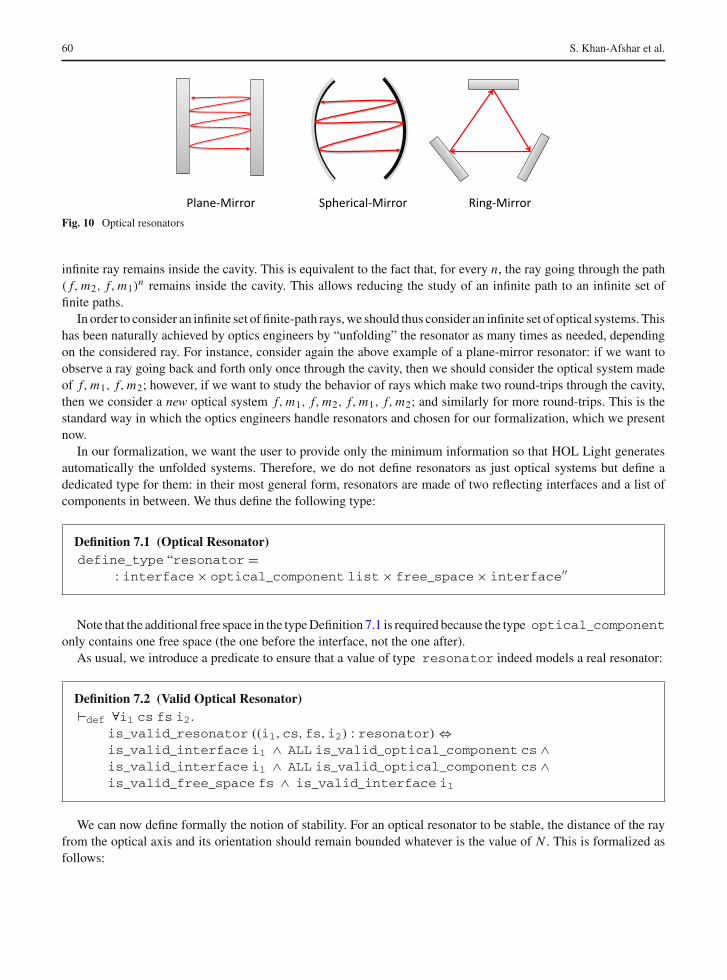
60 S. Khan-Afshar et al.
Fig. 10 Optical resonators
infinite ray remains inside the cavity. This is equivalent to the fact that, for every n, the ray going through the path( f,m2, f,m1)
n remains inside the cavity. This allows reducing the study of an infinite path to an infinite set offinite paths.
In order to consider an infinite set of finite-path rays, we should thus consider an infinite set of optical systems. Thishas been naturally achieved by optics engineers by “unfolding” the resonator as many times as needed, dependingon the considered ray. For instance, consider again the above example of a plane-mirror resonator: if we want toobserve a ray going back and forth only once through the cavity, then we should consider the optical system madeof f,m1, f,m2; however, if we want to study the behavior of rays which make two round-trips through the cavity,then we consider a new optical system f,m1, f,m2, f,m1, f,m2; and similarly for more round-trips. This is thestandard way in which the optics engineers handle resonators and chosen for our formalization, which we presentnow.
In our formalization, we want the user to provide only the minimum information so that HOL Light generatesautomatically the unfolded systems. Therefore, we do not define resonators as just optical systems but define adedicated type for them: in their most general form, resonators are made of two reflecting interfaces and a list ofcomponents in between. We thus define the following type:
Definition 7.1 (Optical Resonator)define_type “resonator =
: interface× optical_component list× free_space× interface′′
Note that the additional free space in the type Definition 7.1 is required because the type optical_componentonly contains one free space (the one before the interface, not the one after).
As usual, we introduce a predicate to ensure that a value of type resonator indeed models a real resonator:
Definition 7.2 (Valid Optical Resonator)�def ∀i1 cs fs i2.
is_valid_resonator ((i1,cs,fs,i2) : resonator) ⇔is_valid_interface i1 ∧ ALL is_valid_optical_component cs ∧is_valid_interface i1 ∧ ALL is_valid_optical_component cs ∧is_valid_free_space fs ∧ is_valid_interface i1
We can now define formally the notion of stability. For an optical resonator to be stable, the distance of the rayfrom the optical axis and its orientation should remain bounded whatever is the value of N . This is formalized asfollows:

Formal Analysis of Optical Systems 61
Fig. 11 Fabry–Pérotresonator
Spherical Mirrors
d
n
R R
Definition 7.3 (Resonator Stability)�def ∀res.
is_stable_resonator res ⇔(∀r. ∃y θ. ∀N. is_valid_ray_in_system r (unfold_resonator res N) ⇒
(let yn, θn = last_single_ray r in abs(yn) ≤ y ∧ abs(θn) < θ))
where, unfold_resonator accepts two parameters, i.e., a resonator ( res) and a number ( N) which specifiesthe number of round trips.
Formally proving that a resonator satisfies the abstract condition of Definition 7.3 does not seem trivial at first.However, if the determinant of a resonator matrix M is 1 (which is the case in practice), optics engineers haveknown for a long time that having −1 < M11+M22
2 < 1 is sufficient to ensure that the stability condition holds. Thiscan actually be proved by using Sylvester’s Theorem [73], which has already been formalized in [68]. Finally, wederive the generalized stability theorem for any resonator as follows:
Theorem 7.1 (Stability Theorem)� ∀res.is_valid_resonator res ∧∀N. let M = system_composition (unfold_resonator res 1) indet M = 1 ∧ −1 <
M1,1+M2,22 ∧ M1,1+M2,2
2 < 1) ⇒ is_stable_resonator res
where Mi,j represents the element at column i and row j of the matrix and det represents determinate of amatrix. The formal verification of Theorem 7.1 requires the definition of stability (Definition 7.3) and Sylvester’stheorem [68]. Note that our stability theorem is quite general and can be used to verify the stability of almost allkinds of optical resonators.
As a direct application of the framework developed in this section, we present the stability analysis of the Fabry–Pérot (FP) resonator with spherical mirrors as shown in Fig. 11. This architecture is composed of two sphericalmirrors with radius of curvature R separated by a distance d and refractive index n.
We formally model this resonator as follows:
Definition 7.4 (FP Resonator)�def ∀R d n.
(fp_resonator R d n : resonator) = (spherical R, [ ], (n,d),spherical R)
where [ ] represents an empty list of components because the given structure has no component between sphericalinterfaces but only a free space (n,d). Next, we verify that the FP resonator is indeed a valid resonator as follows:

62 S. Khan-Afshar et al.
Theorem 7.2 (Valid FP resonator)� ∀R d n. R �= 0 ∧ 0 ≤ d ∧ 0 < n ⇒ is_valid_resonator (fp_resonator R d n)
Finally, we formally verify the stability of the FP resonator as follows:
Theorem 7.3 (Stability of FP Resonator)� ∀R d n.R �= 0 ∧ 0 < n ∧ 0 < d
2 ∧ d2 < 2 ⇒ is_stable_resonator (fp_resonator R d n)
The first two assumptions just ensure the validity of the model description. The two following ones provide theintended stability criteria. The formal verification of the above theorem requires Theorem 7.1 along with somefundamental properties of the matrices and arithmetic reasoning.
This completes our formalization of FP resonator which demonstrates the utilization of our ray optics formaliza-tion. We verified a generic result of stability (Theorem 7.1) for any number of round trips and any considered ray oflight within the resonator. Informally, this is achieved by tracing a single ray for hundreds of simulation runs whichis of-course both time consuming and incomplete. On the other hand, formal verification of stability in a theoremprover provides explicit conditions (in the form of ranges of systems parameters, e.g., Theorem 7.1) under whichthe given resonator can be stable. This can reduce the problem of checking the stability to just the satisfaction ofsuch conditions. We admit the fact that formalization of ray optics requires a significant amount of time along withthe expertise of both HOL and underlying physical concepts. We believe that such efforts paid off when the timerequired to analyze practical applications reduces to the fraction of the time to formalize required HOL theories. Forexample, analysis of FP resonator requires around 150 lines of HOL Light code and 2 man-hours by an expert user.
Apart from the above described application, we have developed a library of frequently used optical components,such as thin lens, thick lens and dielectric plate (detailed description and formalization can be found in [68]). Weshowed the effectiveness of developed theories by the formal analysis of some more practical optical resonators like,Fabry–Pérot resonator with Fiber-rod lens and Z-shaped resonators [67,68]. Moreover, we devised a generalizedprocedure for the formal stability analysis of optical resonators usable by physicists and optical engineers (detailscan be found in [66]).
8 Combining HOL Light and Mechanized Mathematical Systems
The modelling and analysis of optical systems sometimes involves situations where underlying mathematical equa-tions have no closed-form solution. Similarly, such an analysis involves the simplification of complex mathematicalexpressions involving multivariate calculus. The first problem can be addressed by using well-known numericaltechniques which are readily integrated in computational tools such as MATLAB [54]. On the other hand, the lattercan be addressed using computer algebra systems (e.g., Mathematica and Maple) which are considered to be mostefficient tools for computing symbolic solutions automatically. Both of these techniques have some known limita-tion of incompleteness and soundness in case of numerical techniques and computer algebra systems, respectively.In this work, our main idea is to leverage upon the expressive nature and soundness of higher-order-logic theoremproving as much as possible, but at the same time it cannot provide a stand-alone solution. In order to handle thissituation, we propose to provide a bridge connecting theorem provers with symbolic and numerical techniquesbased tools. In this bridge, the given equation is first transferred to a CAS in order to be simplified symbolically. Ifit is successfully simplified, then we transfer it to the theorem prover (ideally by first certifying the simplification)in order to pursue the proof process. In case the equation cannot be simplified symbolically, we have no option butto switch to numerical approaches. Note that all the simplifications are performed by CAS built-in functions andwe do not export axioms and simplification rules of HOL Light.

Formal Analysis of Optical Systems 63
Numericalapproaches
Computer AlgebraSystems
Matlab, Code V,…
Mathematica, Maple,…
Returned result
HOL Light
MathematicalStandard
OpenMath
Fig. 12 Connecting different MMSs using OpenMath
Linking theorem provers with CASs is an active research field, which can be broadly classified into two cate-gories: either both the theorem prover and the CAS directly communicate with each other [14,35,53] or one is builtinside the other [16,43]. Both categories so far cannot provide a rich repository of both axiomatic and algorithmictheories. However, our approach aims at developing a problem-solving environment [17] based on the integrationand interaction between multiple Mechanized Mathematical Systems (MMSs).
Figure 12 explains our proposed architecture where different MMSs are connected. The main goal of our work is todefine a general approach to connect multiple MMSs together in a way to have access to their kernels. This approachprovides us with a large number and a variety of different MMSs like theorem provers, CASs or numerical approacheswith the intention of solving and reasoning over larger sets of problems. We propose to use OpenMath [9] to connectdifferent MMSs. OpenMath is a standard for representing mathematical objects with their semantics, allowing themto be exchanged between computer programs, stored in databases, or published on the worldwide web [9].
As a first step towards our ultimate goal, we established a preliminary link between HOL Light and Mathemat-ica which supports both symbolic and numerical techniques. Figure 13 depicts our methodology to connect HOLLight and Mathematica. This is comprised of three modules: the OCaml units, the XML files which represent theOpenMath objects, and the Java application. It can be observed in Fig. 13 that the connection between each pair ofmodules is bidirectional. This makes the connection between HOL Light and Mathematica complete. If we havea HOL Light goal (or a mathematical expression) which needs to be simplified, we can call the main functioncall_mathematica which accepts two arguments , i.e., the HOL Light expression as a string and the specificMathematica function as a string. Then the HOL Light term is passed to the first module called “Ocaml units”. Itis composed of two components: “Parser & Splitter” and “Parser & Collector”. At this stage, we use the “Parser &Splitter” unit in order to transform the HOL Light term into a corresponding OpenMath object. First, it parses anddecomposes the HOL Light input statement into a list of operators and operands. Then, it maps each element of thelist with the corresponding OpenMath symbol as decoded by means of the related Content Dictionaries (CDs) [7].Finally, it stores the description of the OpenMath object in an XML file. A CD describes the semantics of themathematical object using a collection of symbols, their designations, their formal and informal descriptions, andrules which define the use of appropriate symbols in the correct order. This representation can be exchanged amongseveral systems. The XML file is used as an input for the second module. In addition, the “Parser & Splitter” unitsaves the tag of the specific Mathematica function in a text file in order to be passed to the Java application.
The second module is composed of two XML files that describe the mathematical objects: one file is the HOLLight input statement, the second file is the Mathematica output statement. At this stage we only have the OpenMathobject description of the HOL Light input term. This file represents the input of the third module that contains theJava application which represents the phrasebook [18].
The concept of the phrasebook between OpenMath and Mathematica (available in [11]) was introduced byCaprotti et al. [18]. A phrasebook, by definition, is responsible for the translation of a mathematical expression

64 S. Khan-Afshar et al.
Java Application
OCaml Units
XML Files
Mathematica
HOL Light Input HOL Light Output
Parser & Splitter Parser & Collector
Phrasebook OpenMath-Mathematica
Mathematica Input Mathematica Output
OpenMathContent
Dictionaries
OpenMath
Object Input
OpenMath
Object Output
HOL Light
Fig. 13 Flow of connecting HOL light to mathematica
expressed as an OpenMath object into its representation in the application [17,62], which in our case is Mathematica.This phrasebook is working under the latest version of Mathematica (Mathematica 9.0 [3]). It provides a collection ofencoding and decoding methods between OpenMath and Mathematica based on the declaration of the correspondingCDs. Although it comprises of a large set of useful official and experimental CDs like: arith1, arith2, relation1,etc. [7], it does not include the recent ones such as linalg4 [7], linalgeig1 [8] and relation3 [7]. Before translatingthe XML description into an input Mathematica statement, we need to define the Mathematica calling functionwith the tag already specified by the user. Then, we evaluate it through a connection with MathLink [4], whichopens the Mathematica kernel. Once the result is computed, the Mathematica output statement is translated back toOpenMath; an XML file is generated and passed to the second module which is the XML files. The same processtakes place in the reverse direction until we reach “Parser & Collector” module which translates the OpenMathobject into the specification of the HOL Light symbols in the relevant CDs.
Currently, we have been able to implement different functions such as simplifying transcendental expressions,computing eigenvalues, finding roots and factorization of complex polynomials. For example, we can simplify anexpression as follows:
Input:#call_mathematica “(x pow 2)+ x+ &1 > (x pow 2)+ x+ &2” “Simplify”; ;
Output:val it : thm = � ¬(x pow 2+ x+ &1 > x pow 2+ x+ &2)
Similarly, we can obtain the solution of an equation:
Input:#call_mathematica “x pow 2− &1 = &0” “Solve”; ;
Output:val it : thm = � x pow 2− &1 = &0 �⇒ x = −&1 ∨ x = &1

Formal Analysis of Optical Systems 65
Fig. 14 The system ofinterface
Note that these equations can involve integrals, derivatives and transcendental functions. The current implemen-tation is still experimental and all the source codes and implementation details are available for download at http://hvg.ece.concordia.ca/projects/optics/bridge.htm.
Application: Boundary Condition of an Optical Interface
To show the effectiveness of our approach and implementation to connect HOL Light and Mathematica, in thissection we present the example of a boundary condition computing of an optical interface described with electro-magnetic field.
As mentioned in Sect. 5, to ensure that a system can be expressed in our formal development of electromagneticoptics, it needs to satisfy a set of constraints. For example, in Fig. 14, the system of interface, which includes theinterface i and electromagnetic fields EMF(i), EMF(r), and EMF(t), should satisfy the set of Constraints 5.2.
Our objective is to validate one of the most important predicates of the set of Constraints 5.2:boundary_conditions (Definition 5.2). Noting that the interface in Fig. 14 is the yz-plane, the objectiveis to validate that the electromagnetic fields EMF(i), EMF(r), and EMF(t) satisfy the boundary conditions. This canbe formally described as follows:
Goal 8.1 (Boundary Conditions of the System of Interface in Fig. 14)
∀r t.let θt = arcsin(n1n2 sin θi) in let θr = θi in
let ra = (n2 cos θi −n1 cos θtn2 cos θi +n1 cos θt
)a in let ta = ( 2n2 cos θin2 cos θi +n1 cos θt
)a in
let k(i) = k0n1[cos θi; 0; sin θi] inlet k(r) = k0n1[− cos θr; 0; sin θr] inlet k(t) = k0n2[cos θt; 0; sin θt] inlet E(i) = [0; ae−j (k(i). r−ωt);0] inlet E(r) = [0; rae−j (k(r). r−ωt);0] inlet E(t) = [0; tae−j (k(t). r−ωt);0] inlet H(i) = [a( n1
eta0) cos θi e−j(k(i). r−ωt); 0; −a( n1
eta0) sin θi e−j(k(i). r−ωt)] in
let H(r) = [−ra( n1eta0
) cos θr e−j(k(r). r−ωt); 0; −ra( n1eta0
) sin θr e−j(k(i). r−ωt)] inlet H(t) = [ta( n2
eta0) cos θt e−j(k(t). r−ωt); 0; −ta( n2
eta0) sin θt e−j(k(t). r−ωt)] in
let EMF(i) = plane_wave k(i) ω E(i) H(i) inlet EMF(r) = plane_wave k(r) ω E(r) H(r) inlet EMF(t) = plane_wave k(t) ω E(t) H(t) in∀pt. pt IN (plane_of_interface i) ∧ (pt$1 = 0) ⇒boundary_conditions (EMF(i) + EMF(r)) EMF(t) (plane_of_interface i) r t

66 S. Khan-Afshar et al.
The two variables r and t are indicating points in space and time, respectively. The plane of interface is definedas ∀pt. pt IN (plane_of_interface i) ∧ (pt$1 = 0), which is equivalent to the yz-plane or the planedescribed by “x = 0”. After simplifying the Goal 8.1, we derive the expression shown in Goal 8.2 which, forillustration purposes, we chose to send to Mathematica.
Goal 8.2 (The Expression Sent to Mathematica to be Simplified/Verified)[1;0;0] ccross([0 ;ae−j(k0n1z sin θi−ωt);0] +[0 ; n2 cos θi−n1 cos (arcsin( n1n2
sin θi))
n2 cos θi+n1 cos (arcsin( n1n2sin θi))
ae−j(k0n1z sin θi−ωt); 0]) =[1;0;0] ccross[0 ; 2n2 cos θi
n2 cos θi+n1 cos (arcsin( n1n2sin θi))
a e−j(k0n1z sin (arcsin( n1n2
sin θi))−ωt); 0]∧[1;0;0] ccross([an1
η0cos θie−j(k0n1z sin θi−ωt);0 ;−an1
η0sin θie−j(k0n1z sin θi−ωt)] +
[−n2 cos θi−n1 cos (arcsin( n1n2sin θi))
n2 cos θi+n1 cos (arcsin( n1n2sin θi))
an1η0
cos θie−j(k0n1z sin θi−ωt); 0;
−n2 cos θi−n1 cos (arcsin( n1n2sin θi))
n2 cos θi+n1 cos (arcsin( n1n2sin θi))
an1η0
sin θie−j(k0n1z sin θi−ωt)]) =[1;0;0]ccross[ 2n2 cos θi)n2 cos θi+n1 cos (arcsin( n1n2
sin θi))an2η0
cos (arcsin(n1n2 sin θi)e−j(k0n1z sin (arcsin( n1n2
sin θi))−ωt); 0;− 2n2 cos θin2 cos θi+n1 cos (arcsin( n1n2
sin θi))an2η0
sin (arcsin(n1n2 sin θi))e−j(k0n1z sin (arcsin( n1n2
sin θi))−ωt)]
Note that, in Goal 8.2, the predicate boundary_conditions is reduced to the cross product between thenormal to the interface (i.e., [1;0;0]) and summation of electric fields or magnetic fields at the interface. Now,we can validate the Goal 8.2 by calling Mathematica which returns it as a theorem as follows:
Input:#call_mathematica “Statement of Goal 8.2”“FullSimplify”; ;Output:val it : thm = �[1;0;0] ccross([0 ;ae−j(k0n1z sin θi−ωt);0] + [0 ; n2 cos θi−n1 cos (arcsin( n1n2
sin θi))
n2 cos θi+n1 cos (arcsin( n1n2sin θi))
ae−j(k0n1z sin θi−ωt); 0]) =[1;0;0] ccross [0 ; 2n2 cos θi
n2 cos θi+n1 cos (arcsin( n1n2sin θi))
a e−j(k0n1z sin (arcsin( n1n2
sin θi))−ωt); 0]∧[1;0;0] ccross([an1
η0cos θie−j(k0n1z sin θi−ωt);0 ;−an1
η0sin θie−j(k0n1z sin θi−ωt)] +
[−n2 cos θi−n1 cos (arcsin( n1n2sin θi))
n2 cos θi+n1 cos (arcsin( n1n2sin θi))
an1η0
cos θie−j(k0n1z sin θi−ωt); 0;
−n2 cos θi−n1 cos (arcsin( n1n2sin θi))
n2 cos θi+n1 cos (arcsin( n1n2sin θi))
an1η0
sin θie−j(k0n1z sin θi−ωt)]) =[1;0;0]ccross[ 2n2 cos θi)n2 cos θi+n1 cos (arcsin( n1n2
sin θi))an2η0
cos (arcsin(n1n2 sin θi)e−j(k0n1z sin (arcsin( n1n2
sin θi))−ωt); 0;− 2n2 cos θin2 cos θi+n1 cos (arcsin( n1n2
sin θi))an2η0
sin (arcsin(n1n2 sin θi))e−j(k0n1z sin (arcsin( n1n2
sin θi))−ωt)]

Formal Analysis of Optical Systems 67
The total verification time for this proof on an Intel i7, 2.8 GHz CPU with 32 GB RAM and Oracle Linux 6.3OS was about 3 s, which includes the time to invoke Mathematica and get its feedback. This example illustrates theusefulness of the CAS link that greatly facilitates the interactive theorem proving process by automatically verifyingsome of the proof goals that would have required hours of user guidance if verified by theorem proving alone.
9 Engineering Prospects
The use of formal methods (particularly higher-order-logic theorem proving) in practical engineering system analy-sis is always very challenging. The main reason behind this is the unfamiliarity of formal methods in differentengineering and physical sciences, e.g., control, mechanical and chemical engineering. To the best of our knowl-edge, formal methods have never been used in optical system analysis due to the above mentioned reasons. Inthis paper, we propose theorem proving as a complementary approach to the traditional optical system analysistechniques particularly, simulation and CASs. We believe that we have developed several important libraries fordifferent optics theories to be used in the analysis of practical optical systems such as the design and verification ofoptical resonators (e.g., [67]).
After a detailed investigation of some popular optical system analysis tools [10,12,70,74], we have identifiedsome fundamental requirements that should be considered in a formalization tool. The first requirement is theanalysis capabilities in all three domains, i.e., ray, electromagnetic and quantum optics. We believe that in ourcurrent framework, we have significantly advanced in the fulfilment of this requirement as described in Sects. 4, 5and 6. The second requirement is the availability of the most frequently used components, such as lenses, mirrors,resonators and quantum gates. Such a library can significantly reduce the analysis time which can ultimately assistin reducing the time-to-market of new optical devices. In our current formalization, we have developed librariesof frequently used components in all three domains (i.e., ray, electromagnetic and quantum optics) and this isa continuing process. The third requirement is the facility to define some new component types which can bealtogether a new type or a composition of existing components. Given the expressiveness of higher-order logic andflexibility of our already defined data-types, this goal can easily be achieved in our current framework. But thisrequires sufficient expertise of using our HOL Light developments, which is a drawback in the context of targetedusers of our formalization, i.e., physicists and optical engineers.
Most optical system analysis tools [10,12,70,74] provide significant automation. Due to the undecidable na-ture of HOL theorem proving, this is one of the most challenging requirements. We believe that this particularrequirement depends on the nature of the properties of optical systems that we need to analyze in a theorem prover.For example, proving stability can significantly be automated, but proving the quantum efficiency of a resonatorcannot be performed without user interaction. During our formalization, we tried to automate as much tasks aswe can by developing some automation tactics. For example, in ray optics, VALID_OPTICAL_SYSTEM_TACcan automatically verify the validity of a given optical system. Similarly, we have developed some tactics for theelectromagnetic and quantum optics formalizations which details can be found in our source codes [2].
Another important requirement is to perform computational analysis in case of having no closed-form solutionsand symbolic analysis in case of evaluating some complicated mathematical expressions involving partial differentialequations, eigenvalues and vector integrals. Nowadays, it is a common practice to translate optical system analysisproblems from one tool to another (e.g., [5,6]). Providing such facilities in a formalization tool is not an easy task,however, we propose a preliminary framework to connect different formal and informal tools as described in Sect. 8.Finally, an essential requirement is to build a graphical user interface (GUI) to provide an easy interaction betweenthe user and the HOL Light theorem prover. Such a GUI can be built on arbitrary choices, i.e., text based or usingcomputer aided design (CAD) tools. In each case, the main task is to properly translate the given information (textor a diagram) to match our HOL Light definitions. Recently, we have started focusing in this direction with a goal ofbuilding a tool for the formal stability analysis of optical resonators. The main intention is to assess the feasibilityand use it as a base to build a comprehensive GUI to help researchers and practitioners involved in optical systemanalysis.

68 S. Khan-Afshar et al.
10 Discussion and Conclusion
In this paper, we presented a framework to enhance the verification of optical systems, by introducing the formalanalysis of optical system using higher-order-logic theorem proving as a complementary approach to traditionaltechniques, namely simulation based approaches and CASs. In this regard, we explained how to have both thesystem specification (in terms of properties) and its implementation (in terms of a physical model based on classicaltheories of optics or quantum optics) formalized. We can then verify, in HOL Light, that the implementation impliesall the properties extracted from the specification. Our framework certifies and clarifies the exact logical steps inwhich the physical assumptions and idealizations are pivotal inside each theory. Invariably, such details are implicitor get lost in traditional approaches: one makes assumptions and idealizations exactly to forget about details and toobtain simpler mathematics to work on; using a computer even only to book-keep such details can add significant,reliable and readily usable knowledge to the whole theoretical framework. In our approach, due to the nature offormal reasoning, not only all the details of analysis are explicitly addressed, it guarantees that no assumption canbe contradicted if a design evolves or is included as part of a hybrid system.
In practice, the verification of an optical system might require some modelling involving various theories, in ahierarchical manner; for example, an early analysis and feasibility study is done using ray optics, then an advancedanalysis concerning the properties of light wave is conducted by wave and electromagnetic optics. Finally, if thesystem involves light sources within its configuration then quantum optics is used. Therefore, in order to make thistask easier for verification engineers, we propose to wrap all the above formalizations in a uniform framework andto develop a mechanism to apply different theories on different aspects of a given system. In order to achieve suchcommon front-end, we developed a library of frequently-used optical components which are basic blocks of opticalsystem models. For instance, in ray, wave and even electromagnetic optics, thin lenses, thick lenses and mirrorsare such frequently used components. Some more complex systems can also be considered, e.g., various kinds ofcavities, or resonators. In quantum optics, beam splitters are an example of such a basic component. Since quantumoptics also has lots of other applications, e.g., in quantum computers, various devices like quantum gates (whichare to quantum computers what usual gates are to usual computers) would also be worth adding to such a library.In all cases, since such components are the basic blocks of optical systems, this library will help to formalize newoptical systems. This is utterly important for the practical usability of the library.
Finally, considering the mathematical complexity of optical model analysis, we proposed to develop a bridgebetween HOL Light and Mathematica in order to increase our problem sets. The main advantage of our approach isthat not only we are connecting the formal part of our framework to the one of the best available CASs in Optics, butgiven the popularity of OpenMath standards, we are hoping to have our bridge extended to many different engines,e.g., MuPAD, a symbolic toolbox of Matlab, which has already developed an OpenMath toolbox [56]. However,relying on the results of CASs reduces the degree of accuracy in our approach and the challenge remains to maintainconsistency of formalization in HOL Light while using CASs.
Note that the reported work is a part of our ongoing research project [2] of optical system verification. We believethat our expandable research efforts will result in enriched HOL Light libraries of optics and the development ofsome new proof technologies.
References
1. Allen, L., Angel, R., Rodney, G.A., Mangus, J.D., Shannon, R.R. , Spoelhof, Ch.P.: The Hubble Space Telescope Optical SystemFailure Report. Technical Report, NASA TM-103443, Washington, DC, November 1990
2. Formal analysis of optical systems, Hardware Verification Group, Concordia University. http://hvg.ece.concordia.ca/projects/optics/ (2014). Accessed 20 Mar 2014
3. Mathematica. http://www.wolfram.com/ (2014). Accessed 20 Mar 20144. Mathlink Link. http://reference.wolfram.com/mathematica/guide/MathLinkAPI.html (2014). Accessed 20 Mar 20145. Matlab–codev toolkit. http://opensource.gsfc.nasa.gov/projects/Matlab_Code_V/ (2014). Accessed 20 Mar 20146. Matlab–zemax toolkit. http://opensource.gsfc.nasa.gov/projects/Matlab_Zemax/ (2014). Accessed 20 Mar 20147. OpenMath Content Dictionaries. http://www.openmath.org/cdnames.html (2014). Accessed 20 Mar 2014

Formal Analysis of Optical Systems 69
8. OpenMath Content Dictionary: linalgeig1. http://www.win.tue.nl/~amc/oz/om/cds/linalgeig1.xml (2014). Accessed 20 Mar 20149. Overview of OpenMath. http://www.openmath.org/overview/index.html (2014). Accessed 20 Mar 2014
10. Rezonator. http://www.rezonator.orion-project.org/ (2014). Accessed 20 Mar 201411. Source Code of the Phrasebook Mathematica-OpenMath. http://mathdox.org/new-web/index.html (2014). Accessed 20 Mar 201412. Zemax. https://www.radiantzemax.com/ (2014). Accessed 20 Mar 201413. Baaske, M., Vollmer, F.: Optical resonator biosensors: molecular diagnostic and nanoparticle detection on an integrated plat-
form. Chem. Phys. Chem. 13(2), 427–436 (2012)14. Ballarin, C., Homann, K., Calmet, J.: Theorems and algorithms: an interface between Isabelle and Maple. In: Levelt, A.H.M. (ed.)
Proceedings of the 1995 International Symposium on Symbolic and Algebraic Computation, ISSAC ’95, pp. 150–157. ACM, NewYork, USA (1995)
15. Born, M., Wolf, E.: Principles of Optics Electromagnetic: Theory of Propagation, Interference and Diffraction of Light. CambridgeUniversity Press, Cambridge, UK (1999)
16. Buchberger, B., Craciun, A., Jebelean, T., Kovacs, L., Kutsia, T., Nakagawa, K., Piroi, F., Popov, N., Robu, J., Rosenkranz, M.,Windsteiger, W.: Theorema: towards computer-aided mathematical theory exploration. J. Appl. Logic 4(4), 470–504 (2006)
17. Caprotti, O., Cohen, A.M.: Connecting proof checkers and computer algebra using OpenMath. In: Bertot, Y., Dowek, G., Thery,L., Hirschowitz, A., Paulin, C. (eds.) Theorem Proving in Higher Order Logics. Lecture Notes in Computer Science, vol. 1690, pp.109–112. Springer, Berlin, Heidelberg (1999)
18. Caprotti, O., Cohen, A.M., Riem, M.: JAVA phrasebooks for computer algebra and automated deduction. SIGSAM Bull. 34, 33–37(2000)
19. Chen, K.J., Chen, H.C., Tsai, K.A., et., al.: Light-emitting devices: resonant-enhanced full-color emission of quantum-dot-baseddisplay technology using a pulsed spray method. Adv. Funct. Mater. 22(24), 5137–5137 (2012)
20. Cheng, Q., Cui, T.J., Zhang, C.: Waves in planar waveguide containing chiral nihility metamaterial. Opt. Commun. 274, 317–321(2007)
21. Dirac, P.A.M.: The fundamental equations of quantum mechanics. Proc. R. Soc. A: Math. Phys. Eng. Sci. 109(752), 642–653 (1925)22. Feynman, R.: Simulating physics with computers. Int. J. Theor. Phys. 21, 467–488 (1982)23. Garg, R.: Analytical and Computational Methods in Electromagnetics. Artech House, Norwood, MA, USA (2008)24. Gordon, M.J.C., Melham, T.F.: Introduction to HOL: A Theorem Proving Environment for Higher-Order Logic. Cambridge
Press, Cambridge (1993)25. Griffiths, D.J.: Introduction to Electrodynamics. Pearson Prentice Hall, Upper Saddle River, NJ, USA (1999)26. Griffiths, D.J.: Introduction to Quantum Mechanics. Pearson Prentice Hall, Upper Saddle River, NJ, USA (2005)27. Hadfield, R.H.: Single-Photon Detectors for Optical Quantum Information Applications. Nat. Photonics 3, 696–705 (2009)28. Hales, T.C.: Introduction to the flyspeck project. In: Mathematics, Algorithms, Proofs, volume 05021 of Dagstuhl Seminar
Proceedings (2005)29. Harrison J.: HOL light: a tutorial introduction. In: Formal Methods in Computer-Aided Design, volume 1166 of LNCS, pp. 265–269.
Springer (1996)30. Harrison, J.: Theorem Proving with the Real Numbers (Distinguished dissertations). Springer, Verlag (1998)31. Harrison, J.: A HOL theory of Euclidean space. In: Theorem Proving in Higher Order Logics, volume 3603 of LNCS, pp. 114–129.
Springer (2005)32. Harrison, J.: Formalizing basic complex analysis. In: From Insight to Proof: Festschrift in Honour of Andrzej Trybulec, volume
10(23) of Studies in Logic, Grammar and Rhetoric, pp. 151–165. University of Białystok (2007)33. Harrison, J.: Handbook of Practical Logic and Automated Reasoning. Cambridge University Press, Cambridge, UK (2009)34. Harrison, J.: HOL light: an overview. In: Theorem Proving in Higher Order Logics, volume 5674 of Lecture Notes in Computer
Science, pp. 60–66. Springer (2009)35. Harrison, J., Théry, L.: A skeptic’s approach to combining HOL and maple. J. Autom. Reason. 21, 279–294 (1998)36. Hasan, O., Afshar, S.KH., Tahar, S.: Formal analysis of optical waveguides in Hol. In: Theorem Proving in Higher Order Logics,
volume 5674 of LNCS, pp. 228–243. Springer (2009)37. Hayes, P.R., O’Keefe, M.T., Woodward, P.R., Gopinath, A.: Higher-order-compact time domain numerical simulation of optical
waveguides. Opt. Quantum Electron. 31(9-10), 813–826 (1999)38. Heinbockel, J.H.: Numerical Methods For Scientific Computing. Trafford, Victoria, BC, Canada (2004)39. Hölzl, J., Immler, F., Huffman, B.: Type classes and filters for mathematical analysis in Isabelle/HOL. In: Blazy, S., Paulin-Mohring,
Ch., Pichardie, D. (eds.) Interactive theorem proving. Lecture Notes in Computer Science, vol. 7998, pp. 279–294. Springer, Berlin,Heidelberg (2013)
40. Johnson, S.G., Joannopoulos, J.D.: Block-iterative frequency domain methods for Maxwell’s equations in a planewave basis. Opt.Expr. 8(3), 173–190 (2001)
41. Clarke, E.M. Jr.., Grumberg, O., Peled, D.A.: Model Checking. The MIT Press, Cambridge, MA, USA (1999)42. Afshar S.K., Aravantinos V.: A HOL-Light library for vectors of complex numbers. http://hvg.ece.concordia.ca/code/hol-light/
complex-vectors (2014). Accessed 20 Mar 201443. Kaliszyk, C., Wiedijk, F.: Certified computer algebra on top of an interactive theorem prover. In: Kauers, M., Kerber, M., Miner, R.,
Windsteiger, W. (eds.) Towards Mechanized Mathematical Assistants. Lecture Notes in Computer Science, vol. 4573, pp. 94–105.Springer, Berlin, Heidelberg (2007)

70 S. Khan-Afshar et al.
44. Karimi, M., Abedi, K., Zavvari, M.: Resonant cavity enhanced quantum ring photodetector at 20 µm wavelength. Opt. QuantumElectron. 45(12), 1249–1258 (2013)
45. Kogelnik, H., Li, T.: Laser beams and resonators. Appl. Opt. 5(10), 1550–1567 (1966)46. LASCAD. http://www.las-cad.com/ (2014). Accessed 20 Mar 201447. Leonhardt, U.: Quantum physics of simple optical instruments. Rep. Progr. Phys. 66(7), 1207 (2003)48. Liu, Y., Sarris, C.D.: Fast time-domain simulation of optical waveguide structures with a multilevel dynamically adaptive mesh
refinement FDTD approach. J. Lightwave Technol. 24(8), 3235–3247 (2006)49. Lounis, B., Orrit, M.: Single-photon sources. Rep. Progr. Phys. 68(5), 1129–1179 (2005)50. Mahmoud, M.Y., Aravantinos, V., Tahar, S.: Formalization of infinite dimension linear spaces with application to quantum theory.
In: NASA Formal Methods, volume 7871 of LNCS, pp. 413–427. Springer (2013)51. Malak, M., Pavy, N., Marty, F., Peter, Y., Liu, A.Q., Bourouina, T.: Stable, high-Q Fabry–Perot resonators with long cavity based on
curved, all-silicon, high reflectance mirrors. In: IEEE International Conference on Micro Electro Mechanical Systems, pp. 720–723(2011)
52. Mandel, L., Wolf, E.: Optical Coherence and Quantum Optics. Cambridge University Press, Cambridge, UK (1995)53. Mathscheme. http://www.cas.mcmaster.ca/research/mathscheme/ (2014). Accessed 20 Mar 201454. MATLAB. http://www.mathworks.com/products/matlab/ (2014). Accessed 20 Mar 201455. Mookherjea, S.: Analysis of optical pulse propagation with two-by-two (ABCD) matrices. Phys. Rev. E 64(016611), 1–10 (2001)56. MuPAD. http://www.mathworks.com/discovery/mupad.html (2014). Accessed 20 Mar 201457. Nakazawa, M., Kubota, H., Sahara, A., Tamura, K.: Time-domain ABCD matrix formalism for laser mode-locking and optical
pulse transmission. IEEE J. Quantum Electron. 34(7), 1075–1081 (1998)58. Naqvi, A.: Comments on waves in planar waveguide containing chiral nihility metamaterial. Opt. Commun. 284:215–216, Elsevier
(2011)59. Institute of Quantum Optics at Leibniz University of Hannover. General directives for safety in the institute of quantum optics. http://
www.iqo.uni-hannover.de/fileadmin/institut/pdf/job%20security/3._Sicherheitmerkblatt06012014_engl.pdf (2014). Accessed 20Mar 2014
60. Pereira, A., Ostermann, F., Cavalcanti, C.: On the use of a virtual Mach–Zehnder interferometer in the teaching of quantummechanics. Phys. Educ. 44(3), 281 (2009)
61. Pollock, C.R.: Fundamentals of Optoelectronics. Tom Casson, Chicago, USA (1995)62. Prieto, H., Dalmas, S., Papegay, Y.: Mathematica as an OpenMath application. SIGSAM Bull. 34, 22–26 (2000)63. Ralph, T.C., Gilchrist, A., Milburn, G.J., Munro, W.J., Glancy, S.: Quantum computation with optical coherent states. Phys. Rev.
68, 042319 (2003)64. Saadany, B., Malak, M., Kubota, M., Marty, F.M., Mita, Y., Khalil, D., Bourouina, T.: Free-space tunable and drop optical filters
using vertical Bragg mirrors on silicon. IEEE J. Sel. Topics Quantum Electron. 12(6), 1480–1488 (2006)65. Saleh, B.E.A., Teich, M.C.: Fundamentals of Photonics. John Wiley & Sons, Inc., New York, USA (1991)66. Siddique, U., Aravantinos, V., Tahar, S.: A new approach for the verification of optical systems. In: Optical System Alignment,
Tolerancing, and Verification VII, volume 8844 of SPIE, pp. 88440G–88440G–14 (2013)67. Siddique, U., Aravantinos, V., Tahar, S.: Formal stability analysis of optical resonators. In: NASA Formal Methods, volume 7871
of LNCS, pp. 368–382 (2013)68. Siddique, U., Aravantinos, V., Tahar, S.: On the formal analysis of geometrical optics in HOL. In: Automated Deduction in Geometry,
volume 7993 of LNCS, pp. 161–180 (2013)69. Siegman, A.E.: Lasers. University Science Books, Sausalito, CA, USA (1986)70. Optica Software. http://www.opticasoftware.com/ (2014). Accessed 20 Mar 201471. Song, W.Z., Zhang, X.M., Liu, A.Q., Lim, C.S., Yap, P.H., Hosseini Habib, M.M.: Refractive index measurement of single living
cells using on-chip Fabry–Perot cavity. Appl. Phys. Lett. 89(20), 203901 (2006)72. Su, B., Xue, J., Sun, L., Zhao, H., Pei, X.: Generalised ABCD matrix treatment for laser resonators and beam propagation. Opt.
Laser Technol. 43(7), 1318–1320 (2011)73. Sylvester, J.J.: The Collected Mathematical Papers of James Joseph Sylvester. vol. 4. Cambridge University Press, Cambridge,
UK (1912)74. Synopsys-CODE-V. http://optics.synopsys.com/codev/index.html (2014). Accessed 20 Mar 201475. White, A.G., Jennewein, T., Barbieri, M.: Single-photon device requirements for operating linear optics quantum computing outside
the post-selection basis. J. Modern Opt. 58, 276–287 (2011)76. Tan, M.P., Kasten, A.M., Sulkin, J.D., Choquette, K.D.: Planar photonic crystal vertical-cavity surface-emitting lasers. IEEE J. Sel.
Topics Quantum Electron. 19(4), 4900107–4900107 (2013)77. Tan, S.M.: A computational toolbox for quantum and atomic optics. J. Opt. B: Quantum Semiclass. Opt. 1, 424–432 (1999)78. Ünlü, M.S., Strite, S.: Resonant cavity enhanced photonic devices. J. Appl. Phys. 78(2), 607—639 (1995)79. Wiedijk, F.: A synthesis of the procedural and declarative styles of interactive theorem proving. Log. Methods Comput. Sci. 8(1),
1–26 (2012)80. Wilson, W.C., Atkinson, G.M.: MOEMS modeling using the geometrical matrix toolbox. Technical report, NASA, Langley Research
Center (2005)81. Yin, L., Hong, W.: Domain decomposition method: a direct solution of Maxwell equations. In: Antennas and Propagation Society
International Symposium, IEEE, vol.2, pp. 1290–1293 (1999)