form dot f 1700.7 (8-72) reproduction of completed page authorized
TRANSCRIPT

Technical Report Documentation Page
1. Report No. FHWA/TX-05/0-5176-1 2. Government Accession No. 3. Recipient’s Catalog No.
4. Title and Subtitle Conversion of Volunteer-Collected GPS Diary Data into Travel Time Performance Measures: Literature Review, Data Requirements, and Data Acquisition Efforts
5. Report Date
December 31, 2004
Revised January 31, 2005
6. Performing Organization Code
7. Author(s)
Chandra R. Bhat, Sivaramakrishnan Srinivasan, and Stacey Bricka 8. Performing Organization Report No. 0-5176-1
10. Work Unit No. (TRAIS)
9. Performing Organization Name and Address
Center for Transportation Research The University of Texas at Austin 3208 Red River, Suite 200 Austin, TX 78705-2650
11. Contract or Grant No. 0-5176
13. Type of Report and Period Covered
Research Report (9/1/04–12/31/04)
12. Sponsoring Agency Name and Address
Texas Department of Transportation Research and Technology Transfer Section/Construction Division P.O. Box 5080 Austin, TX 78763-5080
14. Sponsoring Agency Code
15. Supplementary Notes Project conducted in cooperation with the Federal Highway Administration.
16. Abstract
Conventional travel-survey methodologies require the collection of detailed activity-travel information, which impose a significant burden on respondents, thereby adversely impacting the quality and quantity of data obtained. Advances in the Global Positioning System (GPS) technology has provided transportation planners with an alternative and powerful tool for more accurate travel-data collection with minimal user burden. The data recorded by GPS devices, however, does not directly yield travel information; the navigational streams have to be processed and the travel patterns derived from it. The focus of this research project is to develop software to automate the processing of raw GPS data and to generate outputs of activity-travel patterns in the conventional travel-diary format. The software will identify trips and characterize them by several attributes including trip-end locations, trip purpose, time of day, distance, and speed. Within the overall focus of the research, this report describes the data collection equipment specifications, data collection protocols, and data formats, and presents a comprehensive synthesis of the state of the practice/art in processing GPS data to derive travel diaries. This synthesis is intended as the basis for developing input specifications and processing algorithms for our software. A second objective of this report is to identify the data requirements for the software development purposes and document the efforts undertaken to acquire the data.
17. Key Words Household travel surveys, Global Positioning System (GPS), GPS-based travel surveys, GPS data recording formats, Processing GPS navigational data
18. Distribution Statement No restrictions. This document is available to the public through the National Technical Information Service, Springfield, Virginia 22161; www.ntis.gov
19. Security Classif. (of report) Unclassified
20. Security Classif. (of this page) Unclassified
21. No. of pages 62
22. Price
Form DOT F 1700.7 (8-72) Reproduction of completed page authorized


CONVERSION OF VOLUNTEER-COLLECTED GPS DIARY DATA INTO TRAVEL TIME PERFORMANCE MEASURES:
LITERATURE REVIEW, DATA REQUIREMENTS, AND DATA ACQUISITION EFFORTS
Chandra R. Bhat Sivaramakrishnan Srinivasan
Stacey Bricka
Research Report 5176-1
Research Project 0-5176
“Conversion of Volunteer-Collected GPS Diary Data into Travel Time Performance Measures”
Conducted for the
TEXAS DEPARTMENT OF TRANSPORTATION
in cooperation with the
U.S. DEPARTMENT OF TRANSPORTATION
Federal Highway Administration
by the
CENTER FOR TRANSPORTATION RESEARCH THE UNIVERSITY OF TEXAS AT AUSTIN
December 2004
Revised January 2005


v
DISCLAIMERS
The contents of this report reflect the views of the authors, who are responsible for the facts and the accuracy of the data presented herein. The contents do not necessarily reflect the official views or policies of the Federal Highway Administration or the Texas Department of Transportation. This report does not constitute a standard, specification, or regulation.
There was no invention or discovery conceived or first actually reduced to practice in the course of or under this contract, including any art, method, process, machine, manufacture, design or composition of matter, or any new and useful improvement thereof, or any variety of plant, which is or may be patentable under the patent laws of the United States of America or any foreign country.
NOT INTENDED FOR CONSTRUCTION,
BIDDING, OR PERMIT PURPOSES
Chandra R. Bhat Research Supervisor
ACKNOWLEDGMENTS
Research performed in cooperation with the Texas Department of Transportation and the U.S.
Department of Transportation, Federal Highway Administration

vi

vii
TABLE OF CONTENTS
CHAPTER 1 INTRODUCTION................................................................................................. 1 1.1. HOUSEHOLD TRAVEL SURVEY METHODOLOGY....................................................... 1 1.2. CONCERNS REGARDING HOUSEHOLD TRAVEL SURVEY DATA ................................ 2
1.2.1. Trip underreporting ................................................................................................ 3 1.2.2. Incomplete, missing, or inconsistent trip details .................................................... 3 1.2.3. Lack of route choice details .................................................................................... 4
1.3. HOUSEHOLD TRAVEL SURVEY IMPROVEMENTS IN RESPONSE TO CONCERNS .......... 4 1.3.1. Trip underreporting ................................................................................................ 5 1.3.2. Incomplete, missing, or inconsistent trip details .................................................... 5
1.4. APPLICATION OF GPS TECHNOLOGY TO HOUSEHOLD TRAVEL SURVEYS ................ 6 1.5. RESEARCH OBJECTIVES ......................................................................................... 11 1.6. FOCUS AND STRUCTURE OF THE REPORT ............................................................... 12
CHAPTER 2 DATA FOR TRAVEL-DIARY GENERATION.............................................. 13 2.1. EQUIPMENT AND DATA COLLECTION..................................................................... 13
2.1.1. GPS Receiver/Antenna Specifications .................................................................. 13 2.1.2. GPS Receiver Output Formats.............................................................................. 15 2.1.3. Data Logger Specifications................................................................................... 17 2.1.4. Data Collection Protocols .................................................................................... 18
2.2. SUPPLEMENTAL DATA ........................................................................................... 19 2.2.1. Respondent Characteristics .................................................................................. 20 2.2.2. Transportation Roadway Network Data............................................................... 21 2.2.3. Land Use Data ...................................................................................................... 22
2.3. VALIDATION DATA ................................................................................................ 23
CHAPTER 3 PROCESSING GPS NAVIGATIONAL STREAMS....................................... 25 3.1. PREPROCESSING..................................................................................................... 26 3.2. TRIP DETECTION .................................................................................................... 26 3.3. TRIP CHARACTERIZATION...................................................................................... 30
3.3.1. Trip-end (Stop) Locations ..................................................................................... 30 3.3.2. Trip Timing ........................................................................................................... 31 3.3.3. Trip and Activity Purposes.................................................................................... 31 3.3.4. Trip Distances and Speeds.................................................................................... 33 3.3.5. Trip Route ............................................................................................................. 35
CHAPTER 4 DATA REQUIREMENTS AND ACQUISITION EFFORTS ........................ 37 4.1. GPS EQUIPMENT, DATA COLLECTION PROTOCOLS, AND DATA............................. 37 4.2. SUPPLEMENTAL DATA ........................................................................................... 39
4.2.1. Respondent Characteristics .................................................................................. 40 4.2.2. TAZ Boundaries .................................................................................................... 40 4.2.3. Land Use Data ...................................................................................................... 41 4.2.4. GIS Roadway Network Map.................................................................................. 42
4.3. SELF-REPORTED TRAVEL DIARIES: VALIDATION DATA ........................................ 42

viii
CHAPTER 5 SUMMARY AND CONCLUSIONS.................................................................. 43 References……………………………………………………………………………………….45 Appendix A……………………………………………………………………………………...49

1
CHAPTER 1 INTRODUCTION
For nearly fifty years, household travel surveys have been used to document the travel
behavior of regional households as part of long-range transportation planning efforts. The
survey data are used for general planning and policy analysis, as well as to serve as the
foundation for regional travel demand models. Technology advancements have resulted in
changes in household travel survey data collection procedures, the most recent being the
introduction of Global Positioning Systems (GPS) to record travel patterns. The GPS technology
shows promise to minimize costs, while maximizing the volume of travel data collected.
However, the data recorded by GPS devices do not directly yield travel information; rather, the
outputs from these devices are in the form of navigational streams that have to be processed to
derive travel information. The objective of this project is to provide TxDOT with a software and
analysis procedure that translates the GPS data into the traditional travel data format.
The purpose of this chapter is to provide a brief summary of how surveys are conducted
today, discuss the main concerns regarding household travel survey data, identify how the survey
methods and implementation processes have been evolving to address these concerns, and
finally, discuss how GPS technology options can be employed to enhance household travel
survey data collection efforts. This chapter also identifies the overall objectives of the project.
1.1. Household Travel Survey Methodology
As indicated above, the travel behavior and demographic data obtained through
household travel surveys serve as inputs for many transportation planning activities, including
the development of regional travel demand models. The process of data collection entails four
main steps: (1) random selection of regional households to participate in the survey effort, (2)
collection of demographic and work-related information for all household members, as well as
information on household vehicle ownership characteristics, (3) provision of materials to help
participating households record their travel patterns, and (4) retrieval of the recorded travel data.
The earliest travel surveys were conducted in person, with interviewers collecting
demographic information, providing the households with blank trip logs, and returning at a pre-
arranged time to retrieve the completed trip logs. As telecommunications technology became
more prevalent and telephone ownership became more pervasive, the survey method changed to

2
the use of telephones to establish contact with the households. Interviewers mailed out blank trip
log materials to the households, and the households mailed them back, once completed. In the
mid-1990s, technology improvements again resulted in an enhancement, this time with the
advent of computer-aided telephone interviewing (CATI) technology. The CATI programs are
now commonplace and are used to guide interviewers through the survey administration process
by (a) displaying the appropriate survey questions based on responses to prior questions, (b)
employing built-in checks to ensure data are complete and consistent, and (c) providing the
ability to identify and resolve inconsistent responses (see Weiner, 1999 for a more complete
history of US travel surveys).
In terms of the length of the survey period, most travel surveys in the United States are
designed to obtain 24 hours of travel data for participating household members. On the other
hand, 48-hour, weeklong, or even six-week-long surveys are more commonplace in Europe.
Regardless of the length of the survey and the specific data elements obtained, the final survey
data are usually provided in four files: household demographic data, person-level demographic
data, vehicle information, and travel data. The travel data most commonly include the trip origin
and destination, arrival and departure times, mode of travel, and trip purpose. Depending on the
reported mode of travel, more detailed information may be collected as well, such as vehicle
occupancy, amount paid for parking, and transit route and fare. However, travel route traversed
from origin to destination is not a common data item obtained in these surveys.
An important challenge in travel-survey design is to minimize respondent burden, which
plays an important role in determining when to ask specific questions, what level of information
detail to collect, and how precisely to elicit information. In fact, between the recruitment
interview, recording travel details on the travel day, and providing those details back in the
retrieval telephone interview, it is estimated that the average participating household spends at
least an hour on the survey process. Recognizing the respondent burden, most surveys are
designed to collect only the most critical data elements in as simple a way as is possible.
1.2. Concerns Regarding Household Travel Survey Data
Analysts and modelers who work extensively with travel survey data have raised three
major concerns in recent years regarding the completeness and accuracy of household travel
survey data. These are: (1) trip underreporting, (2) incomplete, missing, or inconsistent trip

3
details, and (3) lack of route choice details. Each of these three issues is discussed in turn in the
following three sections.
1.2.1. Trip underreporting
For some time, modelers and analysts have been concerned that respondents, either
because of inaccurate recall or because of time constraints, do not record all their travel during
the assigned travel period. The time burden imposed by the traditional survey method has a
direct impact on trip reporting: the more details requested of the respondent, the greater the time
and effort required of them (Wolf et al., 2003). Of particular concern are trips that are either
short stops made along the way to a main destination (such as stopping to get coffee on the way
to work), complete round trips made at the end of the travel day (such as picking up a child at a
friend’s home), or impulse trips (Bhat and Lawton, 2000; Jones and Stopher, 2003). While at
face value, an occasional missed trip may not appear to warrant concern, each missed trip could
equate to approximately 200 to 500 missed trips once the survey sample is expanded to the
population of interest.
1.2.2. Incomplete, missing, or inconsistent trip details
Stopher and Wilmont (2000) indicate that respondents are sometimes not able to
comprehend survey questions, leading to misreported trip information and/or the need for
extensive data repair. Further, there is always the danger that the respondent neglected to record
critical trip details, such as travel mode, travel times, or trip purposes, when travel data is
retrieved from participating households through a mail-back option. However, since the advent
of CATI technology, the completeness of the travel data has increased substantially with regard
to these data elements. But problems associated with (a) incomplete or missing trips and (b)
inconsistent trip information continue to affect survey data quality, as discussed in the next two
paragraphs.
The main area where incomplete or missing trip information still adversely impacts the
quality of household travel survey data is in location information. Location information is critical
in travel-demand modeling, as all trip origins and destinations are assigned to a traffic analysis
zone (TAZ). Many TAZs are defined by major roadways or natural features, such as rivers or
mountains. Thus, assigning a shopping destination on the wrong side of the road can result in
incorrectly assigning one trip (or 200 or 500 trips when expanded) to the wrong TAZ.

4
Respondents may know how to get to the grocery store, post office, or day care center, but they
do not normally know the address details for those particular locations. Many respondents are
unaware of crossing geopolitical boundaries such as zip codes or TAZs (Stopher and Wilmont,
2000). In addition, if the location is not one they ordinarily visit, they may have trouble linking
it to a specific geographic location.
The concern about inconsistent trip information is primarily associated with the reporting
of travel times. There is a tendency among respondents to round times to the closest 5-minute or
15-minute clock time, resulting in a loss in time resolution. For example, there are higher
proportions of trip departure and arrivals on the hour, half hour, or quarter hour, rather than the
exact minute, say a 7:53 am departure (Battelle, 1997, Murakami and Wagner, 1999).
1.2.3. Lack of route choice details
In balancing respondent burden against obtaining important travel information, most US
travel surveys omit questions regarding travel route. In travel forecasting, route choice is
implemented using network assignment algorithms. These algorithms are based on the
assumption that individuals choose the shortest path for travel. A study undertaken at the
University of Wisconsin (Jan et al., 2000) to evaluate route-choice assumptions made in the
network assignment component of travel demand modeling indicates that the actual chosen paths
are often quite different from the shortest path, even if the travel times along both paths may be
comparable. In addition to use in travel forecasting for urban transportation planning, route
choice information also becomes important for evaluating the impacts of Advanced Traveler
Information Systems (ATIS) on driver behavior, and in air-quality modeling for determining the
spatial distribution of emissions over the network (Wolf et al., 1999). As a consequence of the
reasons discussed above, it is becoming increasingly important to collect travel route
information.
1.3. Household Travel Survey Improvements in Response to Concerns
In response to the above concerns regarding trip reporting completeness and accuracy,
those conducting travel surveys have responded with improved methods and processes. In this
section, a summary of survey improvements in response to each concern is presented. Route
choice is not discussed in this section, as most travel surveys still do not seek to obtain that level
of information.

5
1.3.1. Trip underreporting
The issue of trip underreporting in household travel surveys is of substantial concern
because, as mentioned above, each missed trip can represent 200 to 500 regional trips when the
survey data are expanded. The level of trip underreporting has been reduced through improved
survey design as well as through CATI programming, which allows the interviewers to probe for
commonly missed trips.
The main methodological improvement in survey design is the move from a trip-based
travel diary (asking the respondent to record all trips made) to a place-based or an activity-based
travel diary. In the place-based diary, the respondent is asked to focus on all places visited on the
travel day, while the activity-based diary asks the respondent to record all activities and their
attributes. Both the place-based and activity-based logs have been shown to improve the
proportion of incidental trips reported during the travel day (Bhat and Lawton, 2000; Stopher and
Wilmont, 2000).
In terms of how the surveys are administered, most firms now allow larger households to
mail in the completed travel forms, in order to minimize the potential that respondent fatigue in
reporting travel information over the phone may result in trip underreporting. In addition, follow-
up calls are undertaken to clarify inconsistencies in the data. Further, most CATI software now
permits an interaction between travel records, so that a respondent only has to provide complete
address details once, even if a different household member visits the same location. Finally, the
CATI program can “copy” travel records among those household members that travel together,
thereby reducing the average retrieval interview length from 20 to 25 minutes per person to
about 12 to 15 minutes per person, depending on the data elements being collected.
1.3.2. Incomplete, missing, or inconsistent trip details
Aside from the CATI advancements that check for consistent and complete responses,
there have also been efforts to replace the paper-based travel diaries with electronic travel diaries
(ETDs) and computer-assisted self-interview (CASI) techniques (see Wolf, 2000 and Jones and
Stopher, 2003 for details on the evolution of survey administration techniques). A characteristic
feature of ETDs and CASI programs is the relative ease with which information can be entered
by the respondent. Testing of these user-friendly interfaces with pull-down menu lists and
precoded responses suggests that the data obtained is more complete and more accurate than that

6
written down in the travel diaries. Further, research also suggests that people may be more
willing to report certain kinds of behaviors (especially those that are considered socially
unacceptable) to a computer rather than writing it down or reporting it orally to an interviewer
(Murakami and Wagner, 1999).
With regard to missing or incomplete address (location) information, CATI can be
programmed to obtain enough address “clues” that enable the analyst to impute the location. In
addition, enhanced CATI programs now allow for integrated geocoding efforts. Thus, the
interviewer can locate and confirm a particular location, thereby “filling in the blanks” with the
missing address details. However, these approaches are more costly and increase the survey
interview length, thereby increasing respondent burden and the corresponding probability that
some trips may go unreported.
1.4. Application of GPS Technology to Household Travel Surveys
The above discussion indicates that individual biases, the inability of respondents to
comprehend survey diary questions, and the recall and reporting limitations of respondents can
critically degrade the quality and quantity of information from conventional self-reported
activity/travel surveys. This is primarily because the respondent still needs to expend
considerable time and effort in recalling and reporting detailed travel information. Significant
advances in survey design methods and effective application of CATI software to minimize data
errors have mitigated concerns to some extent, but come at considerable cost. It is in this context
that GPS technology offers a valuable alternative to conventional data-collection approaches.
Specifically, devices called the “GPS receivers,” positioned anywhere on the earth’s surface and
in view of the GPS satellites, are capable of self-determining their locations with a time-of-day
stamp (Wolf, 2004a). Therefore, travel data can be collected by equipping the respondents’
automobiles with GPS receivers and recording the position and velocity of the vehicles
periodically.
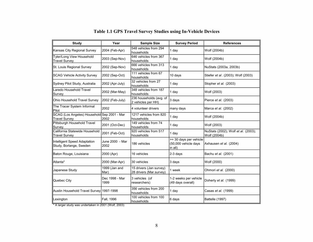
Recent travel-survey studies conducted using in-vehicle GPS devices are presented in
reverse-chronological order in Table 1.1. The early studies conducted at Lexington, Quebec City,
and Atlanta (see bottom of Table 1.1) were aimed at equipment testing to study the relative
performance of different kinds of off-the-shelf GPS devices available in the market. The
Lexington study also explored respondent attitudes to the new GPS technology and the

7
willingness to participate in GPS surveys. The primary focus of the rest of the studies in Table
1.1 has been to compare self-reported travel patterns from conventional travel surveys with
passively recorded travel information from GPS devices. Further, all the studies using in-vehicle
GPS technology, with the exception of the ones undertaken at Lexington and Ohio, have used
passive data collection techniques (i.e., the user intervention is limited to, at most, turning the
device on and off). Studies conducted in Lexington and Ohio, on the other hand, provided the
survey respondents with a non-GPS handheld device to enter information about the trip purpose
and identify the passengers in the vehicle in addition to the use of the in-vehicle GPS device that
passively records vehicle movement. Overall, Table 1.1 clearly reveals the growing interest in
the use of GPS to enhance the completeness and accuracy of travel survey data.
8
Table 1.1 GPS Travel Survey Studies using In-Vehicle Devices
Study Year Sample Size Survey Period References
Kansas City Regional Survey 2004 (Feb-Apr) 548 vehicles from 294 households 1 day Wolf (2004b)
Tyler/Long View Household Travel Survey 2003 (Sep-Nov) 646 vehicles from 367
households 1 day Wolf (2004b)
St. Louis Regional Survey 2002 (Sep-Nov) 666 vehicles from 313 households 1 day NuStats (2003a, 2003b)
SCAG Vehicle Activity Survey 2002 (Sep-Oct) 111 vehicles from 67 households 10 days Stiefer et al . (2003); Wolf (2003)
Sydney Pilot Study, Australia 2002 (Apr-July) 32 vehicles from 27 households 1 day Stopher et al. (2003)
Laredo Household Travel Survey 2002 (Mar-May) 348 vehicles from 187
households 1 day Wolf (2003)
Ohio Household Travel Survey 2002 (Feb-July) 236 households (avg. of 2 vehicles per HH) 3 days Pierce et al. (2003)
The Tracer System Informal Pilot 2002 4 volunteer drivers many days Marca et al. (2002)
SCAG (Los Angeles) Household Travel Survey
Sep 2001 - Mar 2002
1217 vehicles from 820 households 1 day Wolf (2004b)
Pittsburgh Household Travel Survey 2001 (Oct-Dec) 149 vehicles from 74
households 1 day Wolf (2003)
California Statewide Household Travel Survey 2001 (Feb-Oct) 920 vehicles from 517
households 1 day NuStats (2002); Wolf et al. (2003); Wolf (2004b)
Intelligent Speed Adaptation Study, Borlange, Sweden
June 2000 - Mar 2002 186 vehicles
>= 30 days per vehicle (50,000 vehicle days in all)
Axhausen et al. (2004)
Baton Rouge, Louisiana 2000 (Apr) 16 vehicles 2-3 days Bachu et al. (2001)
Atlanta* 2000 (Mar-Apr) 30 vehicles 3 days Wolf (2000)
Japanese Study 1999 (Jan and Mar)
15 drivers (Jan survey) 28 drivers (Mar.survey) 1 week Ohmori et al. (2000)
Quebec City Dec 1998 - Mar 1999
3 vehicles (of researchers)
1-2 weeks per vehicle (49 days overall) Doherty et al. (1999)
Austin Household Travel Survey 1997-1998 356 vehicles from 200 households 1 day Casas et al. (1999)
Lexington Fall, 1996 100 vehicles from 100 households 6 days Battelle (1997)
* A larger study was undertaken in 2001 (Wolf, 2003)

9
In addition to the use of in-vehicle GPS devices for travel data collection, some research
studies have developed and deployed wearable, personal, or handheld GPS units in travel
surveys to collect data on personal travel using any mode of travel. Recent travel surveys using
handheld or personal GPS devices are presented in reverse-chronological order in Table 1.2.
Table 1.2 GPS Travel Survey Studies using Personal/Handheld Devices
Study Year Sample Size Survey Period Reference
Atlanta Route Study 2002 (Nov-Dec) 57 persons 7 days Wolf (2003)
London Study 2002 (Sep-Nov) 154 persons 3 day Steer Davies Gleave (2003)
Atlanta Physical Activity Study 2001-2002 542 persons 2 day Wolf (2003)
Battelle's PTU Development and Testing Study
2000 6 Battelle staff members 2-3 days Battelle (1997)
Netherlands Pilot Study Winter 1998-Spring 1999 151 persons 4 days Draijer et al. (2000)
In the rest of this report, our focus will be on the use of passive in-vehicle GPS devices in
which the user intervention is limited to, at most, turning the device on and off. Such passive in-
vehicle GPS-based travel surveys offer the following advantages over conventional data-
collection approaches:
1. GPS devices can collect data passively and directly record it on electronic media with
little or no intervention from the user, thereby reducing respondent burden substantially.
Consequently, when correctly processed, the GPS technology can address trip
underreporting and can also be effectively used for multiday travel data collection.
2. The location of activities and travel is determined with very high spatial accuracy,
especially after the termination of selective availability in May 2000 (selective
availability (SA) refers to the intentional degradation of GPS spatial accuracy). Thus, the
trip-end locations from GPS surveys are more accurate than the reported locations in
conventional surveys.
10
3. GPS-recorded trip timing data (i.e., time of day of start and end of trips and travel times)
are more accurate than estimates and approximations obtained from conventional
surveys, and do not suffer from round-off errors.
4. GPS technology makes it possible to collect information on the travel route, important
travel information not obtained from current survey techniques.
5. Trip speeds are recorded as actual observations, rather than being calculated as part of the
post-collection processing.
6. Trip distances can be computed accurately using the detailed position data along the
length of the trip.
Overall, it is apparent that almost all the information that can be obtained from
conventional travel surveys (and more) can be derived from passively collected GPS data.
However, despite the several advantages of the GPS survey approaches as discussed above, there
are several issues that need to be addressed for effective use of this new technology for
household travel survey data collection. These are:
1. The GPS data are collected in the form of navigational streams (i.e., periodic recordings
of position and velocity). Substantial processing is necessary to convert these streams
into the conventional travel-diary format for subsequent use of the data for modeling
purposes. Further, the automation of the processing requires operational definitions of
trips and stops. This in turn determines the set of trips and stops that can be identified
from the recorded navigational streams. However, the success of past research in
identifying reported trips from the GPS navigational data streams is very encouraging.
For example, in the St. Louis study (NuStats 2003a, 2003b), about 91% of the trips
reported via a conventional CATI survey were also identified from the GPS data, and in
the California study (Wolf et al., 2003), 1625 of the 1736 (93.6%) CATI-reported trips
were successfully matched to trips identified from GPS data.
2. Equipment specifications (such as errors in position and velocity computations),
operational shortcomings (e.g., loose cabling and loss of signal in regions of dense tree
cover) and respondent error (e.g., forgetting to power on the unit) impact the quality and
quantity of the GPS data collected.
11
3. Trip-purpose information is unknown. This needs to be elicited from the respondent
directly or derived using the GPS data in conjunction with supplemental land use and
network data.
4. The vehicle occupancy levels are unknown; the driver and the passengers in the vehicle
cannot be identified. Such information, if needed, has to be elicited from the respondents
directly.
5. The derived trip diary is an accurate record of the sequence of vehicle trips and not the
person trips. The derived destinations are vehicle trip-end locations. The computed travel
times represent the in-vehicle times and do not include the possible walk times to/from
the vehicle. The actual person trip-end destinations and arrival/departure times associated
with those destinations are unknown or must be imputed in the absence of additional
input from respondents.
1.5. Research Objectives
The discussion presented in the previous section highlights the feasibility of the use of
GPS technology for improving the accuracy and completeness of travel surveys. On the other
hand, it is also evident that the use of passive GPS devices for data collection shifts considerable
burden from the respondent to the analyst. Therefore, the success of this new technology as a
travel survey instrument depends on the ability of the analyst to derive meaningful trip
information from the navigational data streams of GPS devices. All the studies listed in the
previous section have used a mixture of manual and automated procedures for processing GPS
data to derive trip information. In general, these studies have also been largely successful in
identifying CATI-reported trips from the GPS data streams, but little research has been
conducted to date on what the GPS-identified trips that are missing in the CATI data actually
represent.
In a recent review of the state-of-the-art and emerging directions in the application of
new technologies in travel surveys, Wolf (2004b) observes that “recent trends indicate that
someday GPS may be used to replace some or all components of the traditional travel survey
data collection methods”. In such a scenario, in which the data will be collected from several
hundreds of vehicles and/or for multiple days (as opposed to the conventional single-day
approach), there would certainly be a need for robust and efficient algorithms and software for

12
analyzing GPS data streams. Toward this end, the current TxDOT-funded research proposes the
development of a prototype software tool labeled the “GPS-Based Travel-diary Generator”
(GPS-TDG) that automates the process of converting navigational data streams collected
passively from in-vehicle GPS devices into an electronic activity-travel diary. Within this broad
goal, there are four specific objectives for the software:
1. Identify vehicle trips and characterize each trip in terms of attributes such as trip-end
location, trip purpose (or activity type at destination), time of day, duration, distance, and
speed. The derived sequence of trips with all the relevant trip attributes will be written to
an output file in the conventional travel-diary format.
2. Enable the visualization of travel patterns on a GIS platform.
3. Aggregate the derived diary data to generate vehicle trip tables (by trip purpose and time
of day).
4. Compute interzonal network performance measures such as travel times, speeds, and
distances by time of day from the derived diary data.
1.6. Focus and Structure of the Report
The primary aim of this report is to present a comprehensive synthesis of the state of the
art/practice in collecting and processing GPS data. This synthesis forms the basis for developing
input specifications and processing algorithms for the GPS-TDG software. A second objective of
this report is to identify the data requirements for software development purposes and document
the efforts undertaken to acquire the data.
The rest of this report is organized as follows. Chapter 2 describes the structure of the
navigational stream outputs from GPS-based travel-data recording devices. This chapter also
discusses supplemental data that are commonly used along with the GPS navigational streams to
derive the travel patterns. Chapter 3 presents the various processing steps that need to be
undertaken to convert the raw GPS data into a travel-diary format. The algorithms and methods
adopted by past studies for each of the processing steps are also described in this chapter.
Chapter 4 identifies the data requirements for the design and development of the proposed GPS-
TDG software. Efforts undertaken to date to acquire these data are also described. Finally,
Chapter 5 presents the summary and conclusions.

13
CHAPTER 2 DATA FOR TRAVEL-DIARY GENERATION
Passive GPS data collection of travel produces streams of navigational data through
periodic recordings of the position and velocity of equipped vehicles. To facilitate the use of this
data for subsequent analyses, travel-demand modelers and planners need the travel information
to be converted into a conventional trip-diary format (i.e., a sequential listing of all trips
undertaken, with each trip characterized by attributes such as purpose, time of day, trip-end
locations, distance, and duration). This translation from GPS navigational streams to trip
sequences requires an understanding of the GPS equipment specifications, data collection
protocols, and output formats. Also, it is important to note that secondary data, such as
respondent characteristics, roadway network characteristics, and regional land use patterns, can
be used in conjunction with the GPS data to enhance the process of trip-diary generation and to
determine attributes such as trip purpose, which cannot be determined from the GPS data alone.
The objective of this chapter is to present an overview of the GPS outputs and other
secondary data that have been used in prior studies to convert the navigational streams of data
into a trip-diary format. Section 2.1 focuses on the GPS equipment, data collection protocols, and
the formats of the recorded navigational streams. Section 2.2 describes supplemental data that
have been used by analysts for enhancing trip identification and characterization. Finally, Section
2.3 focuses on the data requirements for validating the algorithms developed for trip-diary
generation.
2.1. Equipment and Data Collection
The equipment used in GPS travel data collection typically has two main components: (1)
a GPS antenna and receiver and (2) a data-logging device that records the GPS data. The GPS
receiver/antenna specifications are described in Section 2.1.1. The standard formats of the
outputs from the GPS receivers are next discussed in Section 2.1.2. Section 2.1.3 provides an
overview of the data-logging devices, their operational characteristics, and the data recording
formats and rules. Finally, in Section 2.1.4, two different data collection protocols are presented.
2.1.1. GPS Receiver/Antenna Specifications
There are three important GPS receiver/antenna specifications that are particularly
relevant to the current study from the standpoint of the quality and completeness of the travel

14
data collected. These are (1) the signal acquisition time, (2) position and velocity accuracy, and
(3) the update rate.
The signal acquisition time is the time required by the GPS device to obtain a positional
fix after being powered on. Most GPS devices today have a rated signal acquisition time of 15–
45 seconds (Stopher, 2004). However, this specification assumes that the device is stationary for
this (15–45 seconds) period of time, which is generally not the case in travel survey applications.
Further, the signal acquisition time also depends on how long the device was powered off before
reactivation. For short durations of power off (“warm starts”), the signal acquisition is generally
quicker. However, for long durations of power off (of the order of several hours, “cold starts”),
the signal acquisition time can be much longer. It has been found that, in situations in which the
vehicle is driven almost immediately after ignition on, it may take anywhere between 15 seconds
to 4–5 minutes for signal acquisition, depending on speed of movement and other extraneous
factors, such as the presence of tree canopies and tall buildings (Stopher, 2004). The impact of
the signal acquisition time on the quality of trip attributes recorded (especially trip-end locations
and trip timing) is discussed in detail in Sections 3.3.1 and 3.3.2 of the next chapter.
The second important GPS unit specification is the accuracy of the position and velocity
recordings. With the termination of selective availability in May 2000, the spatial accuracy of
the GPS devices have increased substantially. Today, commercially available GPS devices are
capable of providing a spatial accuracy of about +/- 10 meters (Stopher, 2004). The spatial
accuracy of the GPS device is of particular interest when overlaying GPS streams on a GIS
network map for visualization of travel patterns. The estimation of velocity may involve either
computing the derivative of the position information or using the Doppler shift in the frequency
of the signal due to the relative motion between the satellite and the GPS receiver. The Doppler-
shift based algorithms for speed computation, which are independent of the position information,
have been found to be significantly more accurate compared to those that use the position
information (TRB NCHRP Synthesis, 2001). Most available GPS devices have velocity accuracy
levels of +/- 0.1m/sec (Wolf, 2004a). The accuracy of velocity computations is of particular
interest when the data-logging devices are programmed to record data only if the vehicle
movement is detected (See Section 2.1.3 for further details). The velocity accuracy is also
important from the standpoint of the trip-speed determination.

15
The third specification of interest is the update rate, i.e., how frequently the unit
recomputes the position and velocity. Current GPS units are capable of recomputing and
updating position and velocity information every second. Thus, GPS devices can record travel at
a very fine temporal resolution.
2.1.2. GPS Receiver Output Formats
Most GPS receivers’ output conforms to the National Marine Electronics Association’s
“NMEA 0183 GPS” message formats (Wolf, 2004). These formats represent the ASCII interface
standards for marine electronic devices. The outputs are in the form of a continuous stream of
“sentences,” with each sentence composed of a number of predefined data fields separated by
commas. The sentences begin with a “$” character and end with a “*” character, followed by
check-sum, a carriage return, and a line feed. (The carriage return and line feed are control
characters to signal sentence termination; see Wolf, 2000). The NMEA has prescribed the
standard specifications for many different sentences types, with each sentence type providing
different kinds of data.
The most relevant and commonly used sentence for travel survey purposes is the
“GPRMC” (Wolf, 2004). The sentence specification for GPRMC is presented in a tabular format
in Table 2.1. The GPRMC sentence contains all the necessary position, velocity, and time (PVT)
information required by travel surveys. The position information is recorded in terms of latitude
and longitude in fields 3 through 6. The recording of the latitude and longitude data follows the
“ddmm.mmmm” format, in which the first two digits from the left are the degrees, the next two
are the minutes, and the digits following the period are the decimal minutes. For example, the
value 4533.35 indicates 45 degrees and 33.35 minutes, or equivalently, 45 degrees 35 minutes
and 21 seconds. Velocity is recorded in fields 7 and 8. Field 7 records the speed in knots (1 knot
= 1.5 mph), and the next field contains the direction of movement in degrees. The date and time
are recorded as the Coordinated Universal Time (UTC) or the Greenwich Mean Time (GMT) in
fields 9 and 1. The local time has to be subsequently derived from the UTC by applying
appropriate correction factors. For example, Austin, Texas, is six hours behind the UTC during
winter and five hours behind the UTC during the daylight savings period.

16
Table 2.1 Structure of the GPRMC Sentence
Field Description Format/ Value
0 The entry "GPRMC,” indicating the GPS output sentence structure type GPRMC
1 Time of position fix (in Coordinated Universal Time or Greenwich Mean Time) hhmmss.ss
2 Status (A= valid, V = navigation receiver warning) A/V
3 Latitude ddmm.mmmm
4 Latitude hemisphere (N=North, S=South) N/S
5 Longitude ddmm.mmmm
6 Longitude hemisphere (E = East, W=West) E/W
7 Speed over ground (in knots) 0.0 to 999.9
8 Course over ground (true degrees) 0.0 to 359.9 degrees
9 Date of position fix (in Coordinated Universal Time or Greenwich Mean Time) ddmmyy
10 Magnetic variation 000.0 to 180.0 degrees
11 Magnetic variation direction (E=East, W=West) [west adds to true course] E/W
In addition to the position, velocity, and time (PVT) data, it is also important to consider
information on the reliability and accuracy of the PVT computations. In this regard, there are two
measures of interest: (1) the number of satellites in view and (2) the horizontal dilution of
precision (HDOP). The GPS units require signals from at least three satellites for a two-
dimensional (i.e., latitude and longitude) position computation and signals from four satellites for
a three-dimensional (i.e., latitude, longitude, and altitude) position computation (for further
details on the position computation methodology, see Wolf, 2004). Hence, the number of
satellites in view of the GPS antenna is often used as a measure of validity of the computed
position information. Specifically, the computations are suspect when the number of satellites is
less than three. The second measure of interest, i.e., the HDOP, is a measure of how the satellites
are clustered in the sky as viewed from the GPS antenna when the PVT computations are made

17
(Stopher, 2004). HDOP can take values between 1.0 and 99.9 (Wolf, 2000). Lower values of
HDOP indicate a wider dispersion of the satellites and hence greater reliability of the position
computation. In contrast, higher values of HDOP indicate poor dispersion of the satellites (such
as alignment immediately above the antenna or along the horizon; see Chung and Shalabay,
2004) and hence a lower reliability of the position computation. Data on the number of satellites
in view are recorded in the “GPGSV” sentences, and the HDOP values are recorded in the
“GPGSA” sentences.
2.1.3. Data-Logger Specifications
The second component of the equipment used for GPS travel surveys is a device that
stores the periodic data outputs from the GPS receiver/antenna unit. This data-logging device can
be a personal digital assistant (PDA), a rugged laptop, or a special purpose, purely-passive, data-
logging device such as the GeoLogger (developed by GeoStats) or the GPS Data Logger
(developed by the Institute of Transport Studies, ITS, The University of Sydney). There are two
main specifications of the data-logging devices that are of interest. These are (1) data-logging
formats and rules and (2) operational characteristics.
(1) Data-Logging Formats and Rules
The basic approach to data logging is to simply record the GPRMC sentences output by
the GPS receiver. Hence, the format in which the data are recorded conforms to the GPRMC
sentence specifications. In contrast to the simple recording of GPRMC streams, the GeoLogger
and the GPS Data Logger are special purpose logging devices that have been developed to record
accuracy measures such as the number of satellites in view and HDOP values along with the
relevant fields from the GPRMC sentences (see Wolf, 2004, for GeoLogger output formats and
Stopher, 2004, for GPS Data-Logger output formats). Further, the GeoLogger is also capable of
being programmed to record position information in decimal degrees and speed and altitude
information in metric units. This is important because the ability of the logging devices to
process raw data from the receiver to generate readily usable outputs helps significantly reduce
the preprocessing of data required before being input to the travel-diary generation software. The
preprocessing of data is discussed in more detail in the next chapter.
In addition to alternate formats of data logging, both the GeoLogger and the GPS Data
Logger are capable of being programmed to record data at various preset frequencies (e.g., 1

18
second or 5 seconds). In such a “frequency-based” logging approach, all valid data are recorded
at the preset frequency, irrespective of whether the vehicle is moving or not. In addition, the
GeoLogger is also capable of being programmed to record at the preset frequency only when
movement is detected, i.e., when the speed is greater than 1 mph. This approach is called the
“speed-checked” data logging. The reader will note that the ability to record data only when
motion is detected helps enhance data storage efficiency. The implications of frequency-based
versus speed-checked data logging for processing the data streams for trip-diary generation are
discussed in the next chapter.
(2) Operational Characteristics: User-Flagged versus Purely-Passive Systems
The data logging devices are predominantly powered by their own internal source, such
as a battery. In the case that the data logging device is a PDA or a laptop computer, it may not be
desirable for the system to be powered on all the time. Hence, when such devices are used for
data logging, the user is instructed to power the logger on at the start of the trip and off at the end
of each trip. Such systems are referred to as the “User-Flagged” systems, as the driver flags the
start and end of each trip. In such systems, the data points are necessarily logged only during the
trip and not when the vehicle is at a stop (assuming that the driver diligently turns the PDA off
and on). In contrast to PDAs and pocket PCs, the special purpose data recording devices
developed by GeoStats and ITS Sydney, are constantly powered by internal batteries, and do not
require the user to flag the recording device at the start and end of each trip. Hence, these
systems are referred to as “Purely Passive” systems. In such systems, the data logger records the
points (using any rules as prespecified) as long as the GPS receiver/antenna is powered on.
Hence, in contrast to user-flagged systems, purely passive systems could also be recording points
when the vehicle is at a stop. Thus, the choice of the data logging system has implications for the
structure of the navigational streams recorded by the logging device.
2.1.4. Data Collection Protocols
In addition to equipment specifications and capabilities, GPS data recording patterns are
also impacted by the data collection protocols as determined by the power system characteristics
of the equipped vehicles. Wolf, 2000 and Bachu et al., 2001, have found that, particularly in
American-made automobiles, the power to the cigarette lighter remains on even if the vehicle is
powered off. Since the GPS receiver/antenna unit is typically powered by the vehicle’s power

19
system using a cigarette lighter adapter, there can be two data collection protocols, depending on
the automobile’s power system characteristics, even when the same equipment is used. These are
(1) the “continuous-power” system, in which the cigarette lighter is always powered on and
hence the GPS receiver/antenna unit is also continuously powered on, and (2) the “switched-
power” system, in which the GPS receiver/antenna is powered on and off by powering the
ignition on and off, respectively.
The two data collection protocols have important implications for the nature and structure
of the data outputs. First, the impact of GPS signal acquisition time on the data recordings is
minimal in the case of continuous-power systems, as the GPS receiver is not turned off and on at
each stop. However, for switched-power systems, the impacts of signal acquisition time must
necessarily be considered. Second, in the case of switched-power systems, the data points are not
logged when the vehicle has been powered off at a stop. On the other hand, in the case of
continuous-power systems, the logging of data during the period when the vehicle is off depends
on the logging device specifications. For example, if a user-flagged data logging method is used
in a continuous-power system, then the data points are not recorded at the stops, because the user
powers the data logger off. In contrast, if a purely-passive logger (such as the GeoLogger) is
employed, the data points will be logged even when the vehicle is powered off, unless the device
has been preset to employ speed checks during logging. Thus, the structure of the output
navigational streams recorded by the GPS equipment also depends on the data collection
protocols.
In general, the discussion presented here indicates that the choice of data logging
equipment, along with the data logging rules, operational characteristics, and the data collection
protocols, have a significant impact on the data elements recorded and the structure of the output.
This can limit or enhance the ability of an analyst to convert GPS data into the more traditional
travel survey diary format. GPS data processing algorithms must be designed to account for
these different possible output patterns depending on the data collection protocols and equipment
specifications.
2.2. Supplemental Data
The previous section provided a description of the navigational streams obtained from
GPS devices, which form the fundamental inputs for trip-diary generation. While most of the
20
vehicle trip attributes can be derived from the position, velocity, and time information contained
in the GPS data, the trip purpose is one very important attribute that cannot be determined solely
from the GPS data. It is in this context that supplemental data becomes necessary. In addition to
aiding activity/trip-purpose determination, supplemental data can also be used to enhance the
trip-diary generation process by minimizing detection of false trips and by reducing the number
of missed trips.
The supplemental data that have been used in prior GPS travel survey studies can be
broadly divided into three categories: (1) respondent characteristics, (2) transportation network
data, and (3) land use data. Of the three categories of data, respondent characteristics need to be
elicited from the surveyed individuals, which contribute to respondent burden. In contrast, the
other two types of data are typically available at the disposal of the analyst without further
burden to the respondents. Each of these categories of data and their importance in GPS data
processing is discussed below.
2.2.1. Respondent Characteristics
Since travel surveys using in-vehicle GPS devices focus on the collection of vehicular
travel patterns, the survey respondent in this context is considered to be the primary driver of the
vehicle equipped with the GPS device. In households with a single vehicle shared by multiple
persons, each person is to be considered a respondent. The survey administrators typically collect
data on respondent characteristics via a short survey during the installation/removal of the
equipment or as part of a more formal telephone recruitment effort aided by CATI technology.
There are several respondent characteristics that substantially inform activity/trip-purpose
identification efforts. Perhaps the most fundamental and important data in this context are the
home and work locations of the respondent. As home and work form the majority of the trip-end
locations, the knowledge of residential and work locations substantially reduces the effort in
activity/trip-purpose identification (Wolf, 2000). Further, this is the minimum supplemental
information required to classify the trips into the conventionally used aggregate trip-purpose
categories of: home-based work, home-based other, work-based other, and other purposes. For
the identification of more disaggregate activity/trip purposes, additional data are required in the
form of further queries on frequently visited locations. For example, the Baton Rouge study
queried the respondents for the locations of frequently visited shopping centers (Bachu et al.,

21
2001). Other US studies routinely collect the school address for each student in the household,
which can help identify the most common drop-off/pick-up locations.
In addition to the location information, it is also useful to collect data on key
demographic characteristics, such as the age and gender of the respondent. This information can
provide additional insight to identify the activity type pursued by a respondent. The reader is
referred to Section 3.2.4 for further details on the use of demographic data for activity/trip-
purpose identification.
In future travel surveys using only the GPS component, supplemental data collection
efforts on the respondent characteristics can be expected to be designed so as to balance
respondent burden against data requirements for the desired level of disaggregate activity-
purpose determination. Consequently, the GPS data processing software should also be designed
appropriately and without being overly reliant on respondent characteristics.
2.2.2. Transportation Roadway Network Data
The transportation roadway network data as a Geographic Information System (GIS)
layer is useful for GPS data processing in many ways. First, potential trip-end points identified
from the GPS navigational streams can be overlaid on the GIS road network layer to determine
whether they result from congestion delay or traffic signal points or are true activity stops (See
Axhausen et al., 2004 and Section 3.2 of this report). Second, data on the roadway network are
required for determining the trip route. Specifically, the GPS trace points can be overlaid on the
GIS road network to identify the links traveled during the trip. Processing techniques that have
been used to match GPS traces to network links are discussed in Section 3.3.5. Third, the
availability of the roadway network data aids visualization of the travel patterns. The travel
patterns plotted on a GIS map are very useful if the GPS travel survey also includes a subsequent
prompted recall component for additional data collection (such as purpose and vehicle
occupancy for each trip) and/or for the validation of the processed data by the respondent (such
as verifying whether a trip end was really an activity stop or not). Such an approach was adopted
in the recently conducted Kansas City Regional Household survey (Wolf et al., 2004; NuStats,
2004).
In general, in the United States, the road network GIS layer of the study region is readily
available from local and/or state transportation planning organizations. In the absence of such

22
locally maintained data, one could use the roadway network from the Topologically Integrated
Geographic Encoding and Referencing (TIGER) files (US Census Bureau, 2000). For example,
the Baton Rouge (Bachu et al., 2001) and the Lexington (Batelle, 1997) studies used road
network data built from these TIGER files. However, the road network data from the TIGER
files are known to be, in general, less accurate and more error prone (Wolf et al., 1999; TRB
NCHRP Synthesis, 2001). Commercially available roadway network databases such as the
TeleAtlas’ MultiNet shape file are built using the TIGER files along with aerial photography and
GPS field surveys, thereby leading to enhanced positional accuracy. This database has been used
in the SCAG vehicle activity study (see Stiefer et al., 2003).
The accuracy and scale required of the network data depends considerably on its use in
the GPS processing analysis. Specifically, if the network is to be used primarily for visualization
purposes, then the network maps could be of a lower accuracy and smaller scale. However, for
use in trip detection analysis and trip route determination, more accurate data and larger scale
maps are desirable. Further, in this case, it would also be desirable for the network layer to
contain detailed roadway geometry information as opposed to only the representation of the
center line.
2.2.3. Land Use Data
Land use data are required primarily for activity/trip-purpose identification. As already
discussed, data on the respondents’ home and work locations are adequate to classify the trips
into the conventionally used aggregate activity/trip-purpose categories. However, for the
determination of disaggregate activity/trip purposes (e.g., shopping, recreation, and personal
business) GIS data on the regional land use are required. These data can be in one of two types:
(1) facility location or points of interest (POI) data and (2) zoning data.
The POI data provide the spatial location of the major facilities such as shopping malls,
hospitals, and schools within the region. Axhausen et al. (2004) have used such POI data in their
activity/trip-purpose determination analysis in a study conducted in Europe. In the US context,
the TIGER files provide such facility location data. However, there appears to be no documented
use of this data in activity/trip-purpose identification efforts. Considering this issue, we present a
preliminary analysis of the TIGER files and its applicability for our GPS data processing
requirements in Chapter 4.
23
The second type of land use data, i.e., the zoning data, describes the land use pattern
within each zone or parcel. The usefulness of this type of data depends on the spatial extent of
each zone or parcel and the number of land use types into which these zones may be classified.
The smaller the size of the zones and the greater the number of land use categories, the better are
the data suited for activity-type identification. The research undertaken by Wolf (2000) used a
parcel-level land use data in the proof-of-concept study of trip-purpose identification. This land
use inventory is a database of property polygons and the property center point (when the polygon
data was not available) and was developed by the researchers using tax-assessor property
databases, property boundaries from the counties, and other data. (See Wolf, 2000, for a detailed
description of the development of this land use inventory.)
If the trip-end location identified from the GPS streams can be associated with a specific
facility from the POI data, or if the trip end falls within a zone with a single, well-defined land
use, then the identification of trip purpose using the land use data becomes relatively
straightforward. However, when the trip end is in a zone with mixed land use and/or the trip end
cannot be associated with a unique facility, then the determination of trip purpose becomes more
problematic. Section 3.3.3 in the next chapter presents a detailed discussion on how GPS data
processing algorithms have used the POI and zoning data for trip-purpose determination.
2.3. Validation Data
Validation data are required for the purpose of validating the algorithms developed for
processing the GPS streams. Data on the respondent-reported travel patterns can be compared to
the derived GPS travel patterns to examine the performance of the developed automation
procedures. Insights from such a comparative analysis can also be used for enhancing the GPS
data processing algorithms. As already discussed, almost all GPS travel surveys to date have
undertaken an exercise of comparing reported travel to derived trips. However, it is very
important to note that the primary intent of these studies has not been the validation of general-
purpose software for automating GPS data processing. Rather, the focus has been on auditing
reported travel and examining the extent of underreporting of trips (e.g., Wolf, 2004b).
Comparing the derived trips (or machine-recorded trips) with reported travel for
validation of the processing algorithms is not straightforward because of several reasons. First,
the derived travel patterns are a record of vehicle trips, while the reported travel patterns are a

24
record of person trips. Unless each person uses his/her own vehicle and only makes vehicle trips
during the travel period, matching derived and reported travel can be complicated. Second, the
validity of the trips detected from GPS streams but not reported in CATI retrieval require manual
investigation prior to being flagged as a trip end. Follow-up prompted recall surveys of the
respondents may be required to validate such trips. Such an effort has been undertaken in the
Kansas City Regional Household survey (Wolf et al., 2004). Third, there may be inherent
differences between the recorded travel and the reported travel because of survey administration
protocols. For example, in the Kansas City study (Wolf et al., 2004), persons who drove for a
living were instructed not to report work-related travel in their travel survey. However, such trips
are automatically recorded by the GPS device.
In summary, the above discussion suggests that the validation of the GPS processing
algorithms may require not only reported travel data, but also a follow-up prompted recall data
collection effort and a detailed knowledge of the self-reported and GPS-based travel survey
administration protocols for definitive classification of nonreported “trips”.
25
CHAPTER 3 PROCESSING GPS NAVIGATIONAL STREAMS
The previous chapter described the structure of the GPS navigational stream output as
well as additional data that may be used by the analyst to enrich the generated trip diaries. This
chapter focuses on the processing methods, which use one or more of the supplemental data to
automate the process of deriving the trip sequences from the raw GPS streams. Specifically, this
chapter identifies the major attributes of the trip-diary data to be derived, describes the
algorithms used by past GPS travel survey studies in deriving each of these attributes of interest,
and highlights the advantages and shortcomings of these approaches. At this juncture, it is useful
to point out that the application of GPS to travel surveys is a relatively recent development in
transport modeling. Many of the preliminary studies have used data from a small sample of
vehicles for analysis and therefore have relied upon a mixture of manual and automated
procedures for processing GPS data. With the study size increasing (from a few vehicles to
hundreds and thousands of vehicles and from one-day to multiday data collection), there is a
growing interest in the field to develop robust and efficient algorithms and software for
processing and analyzing GPS data streams.
This chapter comprises three sections. Section 3.1 contains a discussion of preprocessing
the raw data downloaded from the GPS devices and converting it into a format that is readily
usable for further trip-diary generation analysis. This latter analysis procedure involves two
major steps: (1) trip detection and (2) trip characterization. The first step involves the
identification of individual trip segments (or equivalently, stops) from the continuous stream of
GPS navigational data. The second step involves the characterization of each trip in terms of
attributes such as location, timing, purpose, distance, speed, and route. It is useful to note here
that trip detection and characterization are inherently interrelated steps. Specifically,
characteristics of the identified trips might provide clues to the possible existence of other trips,
which also need to be flagged as part of the trip detection processes. Alternatively, attempts to
characterize a trip may suggest that the trip is infeasible and was falsely detected by the previous
trip-identification algorithms. Although the interactive nature of these two steps is recognized,
for ease of presentation, the trip detection and trip characterization methods are discussed
separately in Sections 3.2 and Section 3.3, respectively. The interaction between the two steps
will be suitably incorporated in the GPS-TDG software.
26
3.1. Preprocessing
As a first step toward deriving the trip sequences from the GPS navigational streams, the
data downloaded from the logging devices is first converted to a format that is more readily
usable for subsequent analysis. Typically, the data are downloaded as an ASCII text file that is
then imported into a spreadsheet or a database file for input to trip-diary generation software.
Additional processing of specific data elements may also be necessary, especially if the data
logging simply involves the recording of GPRMC sentences. In this case, the preprocessing of
data would entail: (1) conversion of latitude and longitude into decimal degrees, (2) conversion
of speeds from knots to mph or metric units, and (3) conversion of date and time from UTC to
local date and time. In contrast, when special purpose data logging devices, such as the GeoStats
GeoLogger that can be programmed to record attributes in the required units are used, the
preprocessing effort is minimized. Further, the GeoLogger outputs also include the number of
satellites in view and the HDOP values for each record. In this case, the scope of the
preprocessing task can be extended to flag and investigate the invalid and suspicious data points.
For example, Chung and Shalaby (2004) delete records if the number of satellites is less than
three or if the HDOP value is greater than five. The reader will note that, if only the GPRMC
sentences are recorded, then the accuracy measures are not available. For purposes of this study,
suspicious points will be flagged but not immediately deleted.
3.2. Trip Detection
Almost all earlier studies appear to have developed at least semiautomated procedures for
identifying stops from the GPS navigational streams and breaking the streams into individual trip
segments. A central idea to these procedures is the use of GPS data recordings to identify “dwell
times,” which are defined as periods of nonmovement of the vehicle. If the dwell time exceeds a
certain threshold, called the dwell-time threshold, the presence of a stop and a corresponding trip
is inferred. Thus, the fundamental trip detection procedure requires (1) the specification of a
dwell-time threshold and (2) the logic to identify patterns in the GPS streams indicating
nonmovement of the vehicle.
The dwell-time threshold should be chosen appropriately to identify even short duration
stops (for example, stops for pick-up or drop-off), while at the same time guarding against
detection of false stops (e.g., waiting at stoplights or congestion delays) (Wolf, 2000). It has been
27
found that for most urban areas, the use of 120 seconds as the dwell-time threshold is a
reasonable rule for signaling a (potential) stop, i.e., if the period of vehicle nonmovement
exceeds 120 seconds, then this indicates a stop (Stopher, 2004). However, dwell times of less
than the threshold duration of 120 seconds could be quick stops for purposes such as pick-up or
drop-off of passengers, which would be missed with a strict dwell time threshold for trip
detection. To address these issues, the Trip Identification and Analysis System (TIAS)
proprietary software developed by GeoStats (see Axhausen et al., 2004) uses three thresholds in
its preliminary trip detection procedure. Specifically, the trips are classified as “confident” if the
dwell times exceed 5 minutes, “probable” if the dwell time is between 2 and 5 minutes, and
“suspicious delays” if the dwell time is between 20 seconds and 2 minutes. The “probable” and
“suspicious delay” trip ends are subject to subsequent scrutiny based on the trip characteristics
before being ultimately classified as a trip or not. The trip detection procedure developed by
Stopher and colleagues (see Stopher et al., 2002) uses two thresholds; dwell times of 30 to 120
seconds due to engine turn-off are classified as “potential trip ends” and dwell times of greater
than 120 seconds are designated as “trip ends”. Again, as in the case of the TIAS approach, the
“potential trip ends” are subject to further scrutiny.
The second facet of the trip detection procedure is the identification of nonmovement.
As already discussed in the previous chapter, how vehicular movements and nonmovements are
recorded depends on equipment specifications and data collection protocols. Specifically, there
are two major ways in which nonmovement of the vehicle can be recorded. In switched-power
data collection protocols, or when the logging device is user-flagged or uses speed check rules
for data logging, the data recording stops when the vehicle is not moving. In these situations,
extended periods of nonmovement are necessarily represented by breaks in the record streams.
Therefore, nonmovement for long periods of time can be determined by simply looking for gaps
in the time stamps between successive records (Wolf, 2000). In contrast, if a purely passive data
logger without any speed check rules is used in a continuously powered data collection protocol,
the above logic would not be applicable for detecting nonmovements. This is because, in this
scenario, the data points are being continuously logged, even when the vehicle is at a stop and is
powered off. Similarly, the logic of looking for gaps in the time stamps of the successive
recordings cannot be applied in switched-power data collection protocols with frequency-based
logging rules, to identify stops when the engine is not powered off. In these cases,

28
nonmovements have to be detected by explicitly examining the recorded position and speed data.
Specifically, the detection of stops/trip ends involves identifying a sequence of data records over
a certain period of time during which there is little change in the position of the vehicle and the
speed is zero. The following approach1 suggested by Stopher et al. (2002) can be used as the
implementation logic: If the difference in successive latitude and longitude values is less than
0.000051 degrees (about 7.4 meters), the heading is unchanged or zero, and the speed is zero for
a period of 120 seconds or more, then nonmovement is inferred. The reader will note that this
algorithm cannot detect nonmovements of duration less than 2 minutes. Further, it is also not
guaranteed that the detected nonmovement is necessarily a stop and not a congestion delay or a
long wait at a signal.
The above discussions have focused on using solely the GPS navigation data for trip
detection. In this context, prior research has been largely successful in developing algorithms to
identify stops of durations greater then a certain minimum dwell-time threshold (often 2
minutes). Stops of very short durations, however, are more difficult to identify, particularly when
the vehicle is not powered off at the stop. Further, using only the GPS streams, it is not possible
to guarantee that all trip ends identified are true stops (rather than congestion delays or wait
times at the traffic signals). Supplemental data on transportation network characteristics can be
used to alleviate these concerns and enhance trip detection by minimizing the number of missed
trips and false trips. The TIAS software uses a GIS road network layer for trip-detection
enhancement in two ways (Axhausen et al., 2004): First, “probable trip ends” and “suspicious
delay” points identified from the preliminary trip-detection procedures are overlaid on the GIS
road network, and those that fall within the last 1/3 of a road segment upstream of an intersection
are classified as congestion delay and not considered as trip ends. Second, the software examines
the travel paths for overlaps (i.e., loops in the travel path) and “circuity”. Circuity is defined as a
measure of the extent of directional change occurring during the trip and is computed as the ratio
of the actual travel distance to the Euclidian distance between the trip ends. Points classified as
“suspicious delay” from the preliminary analysis are reclassified as “trip ends” if they fall
strategically on a path with high circuity or overlaps.
1 Stopher’s study employed only switched-power data collection protocols. Hence, this methodology was developed specifically to determine stops occurring without engine power off.

29
Subsequent to trip detection, the next steps in the overall trip-diary generation methods
focus on trip characterization. As already indicated, the characteristics of the identified trips
might provide clues to the possible existence of other trips missed by the trip detection processes.
For example, if the origin and destination locations of a trip are found to be the same, this
suggests the possibility of a missed stop (although this could also be indicative of a purely
recreational trip or an abandoned trip, i.e., a round trip with no apparent purpose; see Axhausen
et al., 2004). In such a scenario, one could examine the specific trip further to determine if there
was a missed stop. Another possible approach would be to examine if there is a reversal in
direction of the vehicle along this trip. Stopher et al. (2002) provide an implementation definition
of reversal as a change in heading between 178 and 182 degrees within 30 seconds. It is also
possible that attempts to characterize a trip may suggest that the trip is infeasible and has been
falsely detected by the previous trip-identification algorithms. Axhausen et al. (2004) reclassify a
trip end as erroneous if the trip duration is less than 30 seconds, the average trip speed is greater
than 50 kmph, or the trip distance is greater than 25 kilometers. Similarly, the SCAG vehicle
activity study (Stiefer et al., 2003) required further examination of trips of duration less than 1
minute or greater than 1 hour and with average speeds less than 5 mph. or greater than 60 mph.
Finally, the above-described methods cannot be applied to scenarios in which stops occur
during a period of signal loss. The following methodology to deal with such situations has been
developed by Stopher et al. (2002):
1. The average speeds immediately before and after the period of signal loss is determined
using the last 10 track points before the period of signal loss and the first 10 track points
after the period of signal loss.
2. The estimated speed during the period of signal loss is determined using the straight-line
distance between the location of signal loss and the location of signal reacquisition
(“signal-loss distance”) and the time period of signal loss.
3. If the estimated speed is considerably lower than the average speeds before and after the
signal loss period, a potential stop is inferred.
4. If a potential stop is inferred, the expected time to traverse the signal-loss distance at the
average speeds prior to the period of signal loss is computed. This is subtracted from the
time period of signal loss to obtain an estimate of the stop duration. If this stop duration is
30
greater than 120 seconds, a stop is inferred; otherwise no stop is assumed to have
occurred.
3.3. Trip Characterization
The second major step in the overall trip-diary generation procedure involves the
characterization of the trips and stops identified by the first step of trip detection. The various
trip attributes that may be derived from the GPS navigational streams and other supplemental
data are the geographic location of the trip ends (Section 3.3.1), trip timing (Section 3.3.2),
activity/trip purpose (Section 3.3.3), trip distances and speeds (Section 3.3.4), and route (Section
3.3.5). It is very important to note that the methods to determine each of these attributes could be
potentially interlinked. For ease in presentation, we discuss the methods to derive each of these
attributes in separate subsections below. However, the GPS-TDG software will suitably
incorporate the linkages when determining the trip attributes, and also include routines to check
for the reasonableness of the overall trip characteristics.
3.3.1. Trip-end (Stop) Locations
Origin and destination trip-end locations may be determined by reading the location
information from the first and last records of the GPS navigational stream corresponding to the
trip. However, when switched-power systems are used, the first valid point recorded may not be
the starting point of the trip due to the time required by the GPS device to acquire a signal. The
severity of this problem (i.e., the magnitude of the distance between the true origin and the
recorded origin) depends on the signal acquisition time of the GPS device used and other factors
(see discussion in Chapter 2). A signal-reception distance analysis undertaken by Bachu et al.,
(2001) indicates that the average distance traveled by a vehicle before the signal is first acquired
is about 0.166 miles (the median value is 0.11 miles). However, this problem can be remedied by
assuming that the origin location of a trip is the same as the destination location of the previous
trip (Schonfelder et al., 2002).
A second issue with trip-end location identification arises specifically in the case of
multiday data collection. When multiday travel data are analyzed, it is possible that the recoded
coordinates of the trip ends are found to be different even if the actual trip destinations are the
same. This could be because of use of different parking spots and/or inherent randomness in the
GPS position determination. Schonfelder and Samaga (2003) have developed an algorithm to

31
identify the main destination locations from a clustered set of trip-end recordings. In this
procedure, for each trip-end location, the distance to all other trip-end locations within a radius
of 200 meters was computed. Those trip ends that have the most neighbors and the smallest
average distance to these neighbors (i.e., the cluster centers) are classified as unique destination
locations. For the remaining, non-central, trip ends (i.e., those trip ends that are not classified as a
unique destination location from the previous step), the nearest cluster center is assigned as the
destination location.
The discussion thus far has focused on the use of latitude and longitude to determine the
trip-end locations. The second approach is to use land use parcel data at the trip end to identify a
probable street address corresponding to the destination. For example, in a study undertaken by
Wolf (2000), the trip-end location was overlaid on a GIS land use and network map to determine
the likely land use parcel associated with the trip end and, hence, the address of the trip end. This
procedure was manual and also involved the visual inspection of the aerial photographs for
determination of trip-end location and examination of the road database to identify the nearest
intersection for address assignment.
3.3.2. Trip Timing
The vehicle trip start time is primarily determined based on when the GPS device
acquires its first fix after the start of the trip (i.e., from the time stamp on the first valid record for
the trip). Similarly, the vehicle trip-end time is the time stamp on the last valid position assumed
to be the end of the trip. Consequently, the determination of the correct trip start times can be
impacted by the signal acquisition time, if switched power systems are used. Further, if there is a
loss of fix at the end of the trip (e.g., driving into a parking garage), the recorded trip end may
not be the true trip end. As a result of these issues, the recorded vehicle trip time can be expected
to be systematically less than the actual vehicle trip time (and the reported person trip time), with
the discrepancy being between several seconds to several minutes (Murakami and Wagner,
1999). Stopher et al. (2002) emphasize the need to develop interpolation methods to determine
the true start times.
3.3.3. Trip and Activity Purposes
The identification of activity/trip purpose is perhaps the most challenging of all GPS data
processing tasks. The first step in this direction was taken by Wolf (2000) in her dissertation

32
research. In this work, she proposed to use land use information at the trip end as the primary
means to identify trip purpose. Specifically, this approach involves a “point-in-polygon” analysis
to first match the trip-end location (a point) to a polygon-based land use inventory to determine
the land use type at the trip end. Further, each land use type was associated with a primary trip
purpose, and whenever possible, secondary and tertiary trip purposes were also identified. The
study employed 25 land use type categories and 11 trip-purpose categories. The land use at the
trip-end location along with the time-of-day of travel, and activity duration at the stop was used
to manually assign trip purposes. The major problem encountered during this step was that it was
not possible to associate certain land use categories (such as mixed-use land parcels and vacant
lots) with a specific trip purpose. Further, the success of this methodology requires a very
detailed land use GIS database at a fine spatial resolution, as was available in Atlanta where
Wolf’s study was undertaken.
The Swiss researchers (see Axhausen et al., 2004; Schonfelder and Samaga, 2003) have
developed the most comprehensive approach for trip-purpose identification to date in the context
of multiday travel-data collection. These researchers have used data on the demographic
characteristics of the survey respondents, POI or facility location data, land use patterns, and
national travel patterns to develop a probabilistic approach to trip-purpose determination. The
overall methodology is summarized here:
1. For trip-end destinations that are within 200 meters of the driver’s household location, the
trip purpose is determined as “home”.
2. For full-time workers, the trip purpose is assigned as work if (a) the destination location
is the second most frequented of all, (b) the structural and temporal characteristics of the
stop are consistent with those determined from the national travel surveys for the work
purpose, and (c) the record is for a weekday.
3. For the trip destinations not classified as either home or work, “most probable” trip
purposes are determined in three different ways:
a. For each trip destination, all points of interest within a catchment area of 300
meters are identified. Each POI is assigned an a priori probability of being
associated with each of several trip purposes. The probability of each trip purpose
is determined as the weighted sum of the individual trip-purpose probabilities

33
associated with each of the POIs within the catchment area. (POIs closer to the
trip destination have a higher weight.) The most probable trip purpose is
determined.
b. The land use patterns within 200 meters of each trip destination are examined.
Each land use class is also assigned an a priori probability of being associated
with each of several trip purposes. The trip-purpose probabilities of all the distinct
land use classes found within the buffer zone are examined to identify the most
probable trip purpose.
c. A third “most probable” trip purpose is determined using the characteristics of the
driver (gender, automobile availability, and employment status) and the temporal
characteristics of the stop (e.g., day of the week, activity start time, and activity
duration). The national travel characteristics are used to develop rules of
association between the demographic characteristics of the driver, the structural
characteristics of the stop, and the trip purpose.
4. The final trip-purpose assignment is accomplished using the three probable trip purposes
identified as follows:
a. If all the three approaches yield the same result for the most probable trip
purpose, then the agreed purpose is assigned.
b. In case of any mismatch, the POI/land use categorization is preferred as the trip
purpose, except when the trip purpose determined from the third method (i.e.,
using demographic characteristics of the driver and the structural characteristics
of the stop) is “pick-up and drop-off,” in which case, this is the assigned trip
purpose.
c. If there is no clear POI/land use assignment possible, the categorization from the
third method is used to determine the trip purpose.
3.3.4. Trip Distances and Speeds
There are two main approaches to determining trip distances from the GPS navigational
data (Battelle, 1997). These are: (1) the point-to-point sum of distances (PP) over the entire trip

34
and (2) the link-to-link sum of distances (LL) over the entire trip after matching the GPS points
to network links.
The first method, i.e., the point-to-point sum of distances, involves the computation of the
distance between successive pairs of recorded locations. These pair-wise distances are then
summed over the entire trip to determine the trip length. The computation of the distance
between successive points may be accomplished using either the latitude and longitude
information for the two points (the formula to calculate this distance is provided by Wolf et al.,
2003) or as a product of the recorded instantaneous speed and the time gap between the
successive data recordings (Wolf, 2000). The primary advantage of the PP approach is that the
trip distance is determined without the use of any secondary data (as would be necessary in the
LL approach discussed in the next paragraph). However, it has been found that the PP approach
could result in the overestimation of trip distances, especially when the position information is
used for computing the distance between successive points in a trip. Specifically, the positional
errors associated with each data record could add up arithmetically leading to overestimation of
the trip length. The magnitude of this error can be particularly large for trip segments through
urban canyons, where multipath errors and satellite line-of-sight issues can significantly
deteriorate the positional accuracy of the GPS points (Wagner et al., 1996). In this context, it has
been suggested (see TRB NCHRP Synthesis, 2001) that the use of positional data recorded every
10 seconds instead of using the data recorded every second (which is the typical recording
frequency) can help reduce the overestimation error by almost 50 percent.
The second method for trip distance computation, i.e., the link-to-link sum over the entire
trip (the LL approach), requires that the GPS traces be matched to an underlying road network to
identify the actual links traveled by the vehicle. The trip length is determined as the sum of the
length of all the roadway links traveled. The advantage of this approach lies in its ability to
accommodate loss of signals midtrip. Specifically, the distance computation using the LL
approach can be accomplished, even when there is a loss of signal for a certain period during the
trip, as long as there are adequate points to identify all the links that have been traversed. The
accuracy of such an approach will depend on, among other factors, the quality and quantity of
valid GPS points available for identifying the network links used (Murakami and Wagner, 1999).
35
The instantaneous speeds are also recorded by the GPS devices. Thus, the average trip
speed and measures of variations in speed along the trip length can be determined in a
straightforward manner from these instantaneous speed measurements.
3.3.5. Trip Route
The trip detection algorithms discussed in Section 3.2 are useful in identifying stops from
the continuous GPS navigational streams. The stream of GPS data records between successive
stops describes the path of vehicular movement during the trip. Hence, the trip route can be
identified using map-matching procedures i.e., matching the GPS data points to appropriate links
on an underlying GIS roadway network map. It is important to note that this matching is not
trivial, as both the GPS data and the digital roadway-network data have different levels of spatial
accuracy and inherent errors. Consequently, the development of map-matching algorithms is in
itself a very vast and complex field of study. Researchers have developed a wide array of
methods using deterministic, probabilistic, and fuzzy-logic-based approaches (see for example,
TRB NCHRP Synthesis, 2001) for matching GPS traces to GIS maps. This report does not seek
to present a comprehensive summary of map-matching procedures, as trip-route determination is
not an objective of this current research project. The reader is referred to the following for some
recent contributions in this area and further references: Chung and Shalaby (2004), Greenfeld
(2002), TRB NCHRP Synthesis (2001), and Doherty et al. (1999).
To summarize, the details provided in this chapter highlight the feasibility of converting
the GPS navigational streams into a more appropriate format for use in analysis of travel
behavior. At the same time, these details also show the specific advantages and disadvantages of
the various procedures available to accomplish the data processing and trip-diary data
generation.

36

37
CHAPTER 4 DATA REQUIREMENTS AND ACQUISITION EFFORTS
The objective of this research effort is to develop the GPS-based Travel-diary Generator
(GPS-TDG) software for processing navigational streams collected from in-vehicle GPS devices
to identify trip sequences and various attributes of each vehicle trip, such as, trip-end locations
(in terms of the Traffic Analysis Zones, or TAZs), trip timings, purpose, distance, and speed. The
generated output will be stored in a conventional travel-diary format. The software will be
capable of displaying the derived travel patterns of individuals either in a tabular format or on a
GIS map. The software will also be designed to aggregate the derived travel patterns of several
individuals to produce interzonal trip tables (by trip purpose and time of day) and network
performance measures such as interzonal travel times, distances, and speeds (by time of day).
Finally, the GPS-TDG will not be strictly tied to the processing of data from any single survey;
rather, it is being developed as general purpose software that can be used for any future GPS
travel survey.
This chapter identifies the data requirements for the development of the GPS-TDG and
describes the efforts undertaken to date toward acquiring relevant data. Section 4.1 describes the
GPS equipment and data collection protocols that we envision that the proposed software will be
capable of handling. The structure of the raw GPS data that has been acquired is also described.
Next, Section 4.2 focuses on supplemental data requirements for GPS-TDG. Finally, Section 4.3
describes the reported travel survey data acquired, which would be used for the validation of the
algorithms developed.
4.1. GPS Equipment, Data Collection Protocols, and Data
The GPS-TDG will be designed to process navigational data collected using a GPS
receiver/antenna with the following specifications:
1. Positional accuracy of 3–5 meters
2. Signal acquisition time: 1 minute (cold) and 15–30 seconds (warm)
3. Update rate of 1 second.
The software will be developed assuming that a handheld device will be used to record
the GPRMC sentence outputs from the GPS receiver. Further, the data logging using the
handheld device is also assumed to be of a “user-flagged” system, i.e., the driver turns the device

38
on at the start of the trip to initiate data recording and turns it off at the end of the trip to
terminate data recording. These equipment and data logging specification assumptions are based
on discussions between the research team and the project director, project coordinator, and other
TxDOT staff involved in this project at a research meeting on December 1, 2004.
For the purposes of use in software development and refinement, we have acquired the
raw GPS outputs from the recently conducted surveys in Laredo and Tyler/Longview. GPS data
from over 100 households (more than 200 vehicles) are available from the Laredo survey, and
data from over 200 households (more than 300 vehicles) are available from the Tyler/Longview
survey. The GPS data for both studies were collected at 1-second logging frequencies, and all
points were logged regardless of speed. The format of the output files is presented in Table 4.1
below (reproduced from the data documentation provided by TxDOT).
Table 4.1 Format of GPS outputs from Laredo and Tyler/Longview surveys
Item#Variable
Name Variable DescriptionData Type Just.
Field Width
Coll. Stage Values
Formal and Full Text
GR-1 RECTYPE Record Type I RJ 1 AGPS Record Type
= 5CORRECTED DATA
GR-2 GPS_IDGPS Receiver Unit ID Number I RJ 3 GPS 0-999
GR-3 HH_ID Household ID Number I RJ 7 A
GR-4 Veh_ID Vehicle Number I RJ 2 A
GR-5 GMT_DATEGreenwich Mean Time Date Stamp I RJ 8 GPS MM/DD/YY
GR-6 GMT_TIMEGreenwich Mean Time Time Stamp I RJ 8 GPS
HH:MM:SS (Military Time)
GR-7 LOC_DATE Local Date Stamp I RJ 8 GPS MM/DD/YY
GR-8 LOC_TIME Local Time Stamp I RJ 8 GPSHH:MM:SS
(Military Time)
GR-9 LAT_RAW Latitude F RJ 16 GPS Decimal DegreesXXX.XXXXXX deg
GR-10 LONG_RAW Longitude F RJ 16 GPS Decimal DegreesXXX.XXXXXX deg
GR-11 ELEV_RAW Elevation F RJ 16 GPS Meters
GR-12 VELOCITY Velocity F RJ 8 GPS Meters/Second 0..514.00m/s
GR-13 HEADING Direction of Vehicle F RJ 6 GPS True North 0.0..359.9 deg
GR-14 HDOPHDOP (horizontal dilution of precision) I RJ 4 GPS 00.5-99.9
GR-15 SATS Number of Satellites I RJ 2 GPS 00-12
It is important to note here that the GPS output formats from the two studies do not
conform to the GPRMC specifications as the special purpose GeoLogger data logging device
was used in these two studies. (See discussions in Chapter 2 for data logging specifications and

39
protocols.) Further, the data recorded by GeoLoggers are also considerably preprocessed, i.e.,
local dates and times are computed, velocity is converted to metric units, and latitude and
longitude values are converted to decimal degrees. Hence, the use of these data for the
development of preprocessing routines would be limited. We hope to acquire additional
navigational data recorded in the GPRMC format using logging devices, which are expected to
be used in future GPS travel surveys to be undertaken by TxDOT. This additional data will be
used in the development of preprocessing routines. Further, the GPS data from the two travel
surveys also contain measures on the quality of the GPS computations for each record, i.e., the
HDOP measure and the number of satellites in view. These measures would not be available if
only GPRMC output would be used in future GPS travel surveys. Hence, the use of these
accuracy measures in our software development would be appropriately limited.
Both the Laredo and the Tyler/Longview surveys collected GPS travel data only for a
single day. Consequently, our ability to develop algorithms that enhance trip detection and
characterization by identifying and examining repetitive patterns from multiday travel-data
collection efforts would be limited.
4.2. Supplemental Data
Based on the detailed discussions provided in the previous chapters, it is clear that the
determination of trip purpose requires supplemental data. Further, the advantages of the use of
supplemental data in enriching the travel-diary generation procedure have also been elaborated in
the previous chapters. In the design of GPS-TDG, the goal is to balance the reliance on
supplemental data (which may not always be possible to obtain or even necessary for the
objectives of any given study) against the benefits (such as disaggregate activity/trip-purpose
determination and enhanced reliability of trip detection) that could be achieved by using the extra
data. Consequently, four categories of supplemental data are identified, two of which are
required inputs for the software, and the other two of which are optional inputs. The required
inputs are data on respondent characteristics and a GIS map of the TAZ boundaries. The optional
inputs are the land use data and roadway network maps. Whenever available, the software uses
these optional inputs to enhance trip detection and characterization. If these inputs are not
provided, the software would still be capable of deriving the travel diary, but without
disaggregate activity purposes and enhanced trip-detection checks. However, for the purposes of

40
software development, all four inputs are required. Each of the four input types is discussed
below.
4.2.1. Respondent Characteristics
The most fundamental respondent characteristics required are the home and work
locations, used to classify the trips into one of the four commonly used aggregate categories:
home-based work, home-based other, work-based other, and other. TxDOT has provided
household and personal characteristics data of the respondents participating in the Laredo and
Tyler/Longview GPS surveys to the research team. The data sets were provided in an ASCII
format, along with the record layout documentation necessary to import the data into analysis or
mapping software. The demographic data, which consists of the household, person, and vehicle
information, are nested in one file, with a record type indicator to help import the data correctly.
The household file contains the home address zip code, the corresponding TAZ, and the
latitude/longitude coordinate. The person file contains similar data for the work address. Thus,
the most fundamental respondent characteristics required for aggregate trip-purpose
determination are available. The demographic data files from the Laredo and Tyler/Longview
surveys also include several household-level (such as number of vehicles, income, and tenure)
and person-level (such as age, gender, and ethnicity) characteristics. The research team will
examine these demographic data and identify the demographic attributes of primary interest for
deriving the travel diaries in subsequent project tasks.
Finally, when collecting data on respondent characteristics, it would also be very useful
to record whether the vehicle equipped with the GPS device has continuous power to the
cigarette lighter or not. In the case of the Laredo and Tyler/Longview surveys, this information
was recorded in “administrative data files,” which are available to the UT research team.
4.2.2. TAZ Boundaries
A GIS map of the TAZ zone boundaries of the study is required for two purposes. First,
the trip-end locations need to be characterized in terms of the TAZs, in addition to latitude and
longitude, for subsequent use in travel modeling. Second, this GIS layer is also needed for the
visualization of travel patterns. The GIS zone boundary layers for Laredo and Tyler/Longview
study area will be acquired from TxDOT.

41
4.2.3. Land Use Data
The land use data are of primary importance for the purpose of disaggregate activity/trip-
purpose determination. There are two types of land use data: (1) the zoning data and (2) facility
location data. Based on preliminary investigations, it appears that land use data at the parcel level
might be the best zoning data available for the purposes of this project. Efforts are underway to
determine whether these data are available for the Laredo and Tyler/Longview study areas.
Further, the research team will also investigate the availability of such data for other regions of
Texas, including the typical land use classifications and data formats adopted by the different
regions.
The second type of land use data are the facility location data (also called the points of
interest data [POI]). In this context, the TIGER/Line files are relevant to this research project.
These files constitute digital databases of geographic features (e.g., roads, railroads, rivers, lakes,
legal boundaries, and census statistical boundaries) with latitude-longitude coordinates, feature
name, and classification, etc. (US Bureau of Census, 2000). These files are available for most
counties in the US. Among the 17 different TIGER/Line files available, the landmark file or
Record Type 7 (US Bureau of Census, 2000) is of particular interest in the context of trip-
purpose identification. Specifically, this file is a record of several regional landmarks, with each
landmark characterized by the landmark name, its geographic location in decimal degrees, a
feature class code, and an identification number. The landmark can either be a point, a line, or an
area type, depending on the size of the feature and the depiction of the feature in the source
document. For example, an airport might appear as a specific point, a line, or an area. Landmark
names are not standardized and may be referenced by variant spellings or different census feature
class codes (CFCC). The major CFCC categories are military installations, multi-household or
transient quarters, custodial facilities, educational or religious institutions, transportation
terminals, employment centers (including shopping centers and office parks), towers, open
space, and special purpose landmarks, such as the post office and police station.
The benefits to using the landmark files for this project include the fact that these data are
readily available for all counties in Texas and can be used by most GIS software packages. In
contrast, a major shortcoming of these files is the omission of key landmarks. A review of the
file for Travis County indicates that the data does contain many familiar landmarks like the
Barton Creek Mall and various apartment complexes. However, the school listings are not

42
complete, nor are the hospitals. (Currently, there are 201 landmarks in all for Travis County; the
entire table is included as Appendix A.) However, there is a project under way at the Census
Bureau (MAF/TIGER Modernization Project) aimed at increasing the completeness of this file.
A second major limitation of the landmarks file is that some addresses are geocoded to the
centroid of the zip code. This causes several landmarks to be “stacked up” at a particular point.
The research team will undertake a more comprehensive assessment to determine the
applicability of the landmarks files for trip-purpose identification.
4.2.4. GIS Roadway Network Map
The next data requirement for the purposes of software development is the GIS roadway
maps of the study regions. Determination of trip route is not a focus of this research project.
Consequently, the predominant use of the road network data is to enhance trip detection by
minimizing the detection of false trip ends (for example stoppage at a signalized intersection).
The research team plans to acquire the roadway network maps developed by TxDOT for the two
study regions (i.e., Laredo and Tyler/Longview) for the purposes of software development.
4.3. Self-Reported Travel Diaries: Validation Data
The final data requirement pertains to the validation of the procedures for the automation
of travel-diary generation. For this purpose, the self-reported travel diaries of the respondents
participating in the GPS and household travel surveys in the Laredo and Tyler/Longview study
areas have been acquired. As discussed in Section 2.3, a detailed knowledge of the survey
administration procedures for both the self-reported and GPS components is very important for
developing validation rules. Correspondingly, the research team plans to acquire detailed
documentation on the survey administration protocols from TxDOT. Finally, it is useful to point
out here that the availability of GPS-recorded and reported travel data from two different studies
provides us with a unique opportunity to test the transferability of our data processing
algorithms. The reader will note that the transferability of the underlying algorithms is important
to the successful development of such general purpose software as the GPS-TDG.
43
CHAPTER 5 SUMMARY AND CONCLUSIONS
Household travel survey data constitute a fundamental input to travel-demand model
development for use in transportation planning and policy analysis. Although the design of
surveys has been enhanced over the years to facilitate a more complete recollection of travel, and
the advancements in the field of computers and telecommunications are being exploited to make
data recording easier and more accurate, there are still several concerns about the data quality
obtained from conventional household travel surveys. These concerns are primarily associated
with the challenge of requiring respondents to record details about all trips and activities for the
designated travel survey period.
Advances in Global Positioning System (GPS) technology has provided transportation
planners with an alternative and powerful tool for more accurate travel-data collection with
minimal user burden and thereby address the concerns of the conventional household travel
surveys. The data recorded by GPS devices, however, does not directly yield travel information;
the navigational streams have to be processed and the travel patterns derived from it. The focus
of this research project is to develop software, called GPS-TDG, to automate the processing of
raw GPS data and to generate outputs of activity-travel patterns in the conventional travel-diary
format. The software will identify trips, and characterize them by several attributes including
trip- end locations, trip purpose, time of day, distance, and speed. The results will be presented to
the analyst in a tabular form and/or on a GIS map, as desired. Further, the software will also be
capable of aggregating the derived trip-diary data to produce trip tables and to compute inter-
zonal network performance measures.
Within the overall focus of the research, this report presented a comprehensive synthesis
of the state of the practice/art in collecting and processing GPS data. This synthesis is intended
as the basis for developing input specifications and processing algorithms for our GPS-TDG
software. A second objective of this report is to identify the data requirements for the software
development purposes and document the efforts undertaken to acquire the data.
Chapter 2 presents an overview of the GPS outputs and other secondary data that has
been used by past GPS travel studies in deriving the trip diaries. Specifically, the GPS
equipment, data collection protocols, and the formats of the recorded navigational streams are
discussed. Further, supplemental data such as respondent characteristics, land use patterns, and

44
roadway network data that have also been used by analysts for enhancing the trip identification
and characterization are described. Finally, the data requirements for validating the algorithms
developed for trip-diary generation are presented.
Chapter 3 presents a comprehensive synthesis of knowledge on the techniques that have
been employed to convert the GPS streams into the travel-diary format. Specifically, we identify
two major steps involved in the trip-diary generation procedure: (1) trip detection and (2) trip
characterization. Trip detection involves the identification of individual trip segments (or
equivalently, stops) from the continuous stream of GPS navigational data, whereas trip
characterization determines attributes of the trips, such as location, timing, purpose, distance,
speed, and route. The trip detection and trip characterization methods adopted by past research
are discussed in detail. In addition, this chapter also discusses preprocessing routines required to
convert the raw GPS streams downloaded from the data loggers to more readily usable formats
for subsequent trip-diary generation analysis.
Chapter 4 focuses on the data requirements for the development of GPS-TDG. The GPS
receiver/antenna and the data logger specifications supported by the software are first discussed.
Next, supplemental data requirements are presented. In the design of GPS-TDG, we seek to
balance the over reliance on supplemental data against the benefits that could be achieved by
using the extra data. Consequently, we identify four categories of supplemental data, two of
which are required inputs for the software application, while two are optional inputs. The
required inputs are data on respondent characteristics and a GIS map of the TAZ boundaries. The
optional inputs are the land use data and roadway network maps. In addition to the GPS and the
supplemental data, we also require self-reported travel data from the GPS survey respondents for
the purposes of validation of the algorithms developed. Chapter 4 also describes our data
acquisition efforts to date. We have obtained the GPS navigational data, the corresponding
reported travel diaries, and data on demographic characteristics of the respondents from the
Laredo and the Tyler/Longview surveys. The research team has also undertaken a preliminary
examination of the applicability of the facility location data from the US Census TIGER files for
the trip-purpose determination. Efforts to acquire supplemental land use and roadway network
data are under way.
45
References Axhausen, K. W., Schonfelder, S., Wolf, J., Oliveria, M., Samaga, U. (2004) “Eighty Weeks of
GPS Traces, Approaches to Enriching Trip Information”, Transportation Research Board 83rd Annual Meeting Pre-print CD-ROM.
Bachu, P. K., Dudala, T., and Kothuri, S. M. (2001) “Prompted Recall in Global Positioning System Survey: Proof-of-Concept Study”, Transportation Research Record 1768, pp 106–113.
Battelle (1997) “Global Positioning Systems for Personal Travel Surveys Lexington Area Travel Data Collection Test-Final Report” prepared for the FHWA, USDOT. www.fhwa.dot.gov/ohim/lextrav.pdf, accessed on March 12, 2004.
Bhat, C. R. and K. Lawton (2000) “Passenger Travel Demand Forecasting”, Transportation in the New Millennium, Transportation Research Board, Washington, D.C.
Casas, J. and Arce, C. H., (1999) “Trip Reporting in Household Travel Diaries: A Comparison to GPS Collected Data”, Transportation Research Board 78th Annual Meeting Pre-print CD- ROM.
Chung, E. and Shalaby, A. (2004) “Development of a Trip Reconstruction Tool to Identify Traveled Links and Used Modes for GPS-Based Personal Travel Surveys”, Transportation Research Board 83rd Annual Meeting Pre-print CD-ROM.
Doherty, S. T., Noel, N., Lee-Gosselin, M. L., Sirios, C., and Ueno, M. (1999) “Moving Beyond Observed Outcomes: Integrating Global Positioning Systems and Interactive Computer-Based Travel Surveys”, In the Proceedings of the Transportation Research Board Conference on “Personal Travel: The Long and Short of It”, Washington D.C.
Draijer, G., Kalfs, N., and Perdok, J. (2000) “GPS as a Data Collection Method for Travel Research: The use of GPS for data collection for all modes of travel”, Transportation Research Board 79th Annual Meeting Pre-print CD-ROM.
Greenfeld, J. S. (2002) “Matching GPS Observations to Locations on a Digital Map” Transportation Research Board 81st Annual Meeting Pre-print CD-ROM.
Jan, O., Horowitz, A., and Peng, Z. (2000) “Using GPS Data to Understand Variations in Path Choice” Transportation Research Board 79th Annual Meeting Pre-print CD-ROM.
Jones, P. M. and P. R. Stopher (2003). Transport Survey Quality and Innovation, Pergamon Press, Elsevier Science.
Marca, J. E., Rindt, C. R., and McNally, M. G. (2002) “The Tracer Data Collection System: Implementation and Operational Experience”, UCI-ITS-AS-WP-02-2, University of California at Irvine.
Marca, J. E., Rindt, C. R., McNally, M. G. (2003) “Collecting Activity Data From GPS Readings”, Transportation Research Board 82nd Annual Meeting Pre-print CD-ROM.
Murakami, E. and Wagner, D. P. (1999) “Can Global Positioning System (GPS) Improve Trip Reporting?” Transportation Research Part C, No 7, pp 149–165.

46
Murakami, E., Wagner, D. P., and Neumeister, D. M. (2000) “Using Global Positioning Systems and Personal Digital Assistants for Personal Travel Surveys in the United States”, Transport Surveys: Raising the Standard, Proceedings of an International Conference on Transport Survey Quality and Innovation, TRB Transportation Research Circular E-C008, pp. iii-B/1 – iii-B/21. http://gulliver.trb.org/publications/circulars/ec008/session_b.pdf, accessed February 23, 2004.
NuStats (2003a) “Household Travel Survey: Final Report of Survey Methodology”, http://www.teamstl.org/library/St_Louis_Final_Methods_Report.pdf, accessed March 12, 2004.
NuStats (2003b) “Household Travel Survey: Final Report of Survey Results”, http://www.teamstl.org/library/St_Louis_Final_Analysis_Report.pdf, accessed March 12, 2004.
NuStats (2002) “2000–2001 California Statewide Household Travel Survey Final Report”, http://www.dot.ca.gov/hq/tsip/TSIPPDF/2000_Household_Survey.pdf, accessed March 12, 2004.
Ohmori, E., Muromachi, Y., Harata, N, and Ohta, K. (2000) “Travel Behavior Data Collected Using GPS and PHS, Traffic and Transportation Studies”, Proceedings of ICTTS 2000, pp.851-858. http://ut.t.u-tokyo.ac.jp/members/nobuaki/ICTTS00.pdf, accessed December 14, 2004.
Pierce, B., Casas, J., and Giaimo, G. (2003) “Estimating Trip Rate Under-Reporting: Preliminary Results from the Ohio Household Travel Survey”, Transportation Research Board 82nd Annual Meeting Pre-print CD–ROM.
Schonfelder, S., Axhausen, K. W., Antille, N., Bierlaire, M. (2002) “Exploring the potentials of automatically collected GPS data for travel behavior analysis – A Swedish data source”, http://roso.epfl.ch/mbi/papers/schoenfelder.pdf, accessed November 29 2004.
Schonfelder, S., and Samaga, U. (2003) “Where do you want to go today? – More observations on daily mobility”, presented at the 3rd Swiss Transport Research Conference (STRC), March, 2003. http://www.strc.ch/Paper/Schoen.pdf, accessed November 28, 2004.
Steer Davies Gleave & GeoStats (2003) “The Use of GPS to Improve Travel Data: Use of GPS in Travel Surveys” Study report prepared for DTLR New Horizon Program. http://www.geostats.com/papers/use%20of%20GPS%20to%20improve%20travel%20data.pdf, accessed on March 12, 2004.
Stiefer, P., Coe, D., Wolf, J., and Oliveria, M. (2003) “Investigating the Impact of Driving Activity on Weekend Ozone Levels using GIS/GPS Technology”, http://www.geostats.com/papers/wolf0396.pdf, accessed on March 12, 2004.
Stopher, P. R. (2004) “GPS, Location, and Household Travel”, in Handbook of Transport Geography and Spatial Systems, Edited by Hensher, D. et al., Elsevier Ltd., pp 432–449.
Stopher, P. R., Bullock, P. J., and Horst, F. N. F. (2003) “Conducting a GPS Survey with a Time-Use Diary”, Transportation Research Board 82nd Annual Meeting Pre-print CD-ROM.
47
Stopher, P. R., Bullock, P., and Jiang, Q (2002) “GPS, GIS and Personal Travel Surveys: An Exercise in Visualization”, presented at the 25th Australian Transport Research Forum, Canberra, Australia, http://www.btre.gov.au/docs/atrf_02/papers/57Stopher%20GPS.pdf, accessed March 12, 2004.
Stopher, P. R. and Wilmot, C. G. (2000) “Some New Approaches to Designing Household Travel Surveys- Time-Use Diaries and GPS”, Transportation Research Board 79th Annual Meeting Pre-print CD-ROM.
TRB NCHRP Synthesis (2001) “Collecting, Processing, and Integrating GPS data into GIS: A Synthesis of Highway Practice”, NCHRP Synthesis 301, Transportation Research Board National Research Council.
US Bureau of Census (2000) “Redistricting Census 2000: TIGER/Line files technical documentation”, US Bureau of Census, http://www.census.gov/geo/www/tiger/rd_2ktiger/tgrrd2k.pdf, accessed December 14, 2004.
Wagner, D. P., Neumeister, D. M., and Murakami, E., (1996) “Global Positioning Systems for Personal Travel Surveys”, paper presented at the National Traffic Data Acquisition Conference (NATDAC), May 1996, Albuquerque, New Mexico.
Weiner, E. (1999) Urban Transportation Planning in the United States, Praeger, Westport, CT.
Wolf, J. (2004a) “Defining GPS and its Capabilities”, in Handbook of Transport Geography and Spatial Systems, Edited by Hensher, D. et al., Elsevier Ltd., pp 411–431.
Wolf, J. (2004b) “Applications of New Technologies in Travel Surveys”, International Conference on Transport Survey Quality and Innovation”, Costa Rica, August, 2004. http://www.its.usyd.edu.au/isctsc/costarica_papers/resource/B4%20-%20Resource%20Wolf.pdf, accessed December 14, 2004.
Wolf, J., Bricka, S., Ashby, T., and Gorugantua, C. (2004) “Advances in the Application of GPS to Household Travel Surveys”, National Household Travel Survey Conference, Washington DC, 2004, http://trb.org/conferences/nhts/Wolf.pdf, Accessed December 14 2004.
Wolf, J. (2003) “Tracing People and Cars with GPS Diaries: Current Experience and Tools” presentation at ETH, Zurich, http://www.ivt.baum.ethz.ch/allgemein/wolf_030228.pdf, accessed on March 12, 2004.
Wolf, J. (2000) Using GPS Data Loggers to Replace Travel Diaries In the Collection of Travel Data, Dissertation, Georgia Institute of Technology, Atlanta.
Wolf, J., Hallmark, S., Oliveria, M., Guensler, R., and Sarasua, W. (1999) “Accuracy Issues with Route Choice Data Collection Using GPS”, Transportation Research Board 78th Annual Meeting Pre-print CD-ROM.
Wolf, J., Oliveira, M., and Thompson, M. (2003) “The Impact of Trip Underreporting on VMT and Travel Time Estimates: Preliminary Findings from the California Statewide Household Travel Survey GPS Study”, Transportation Research Board 82nd Annual Meeting Pre-print CD-ROM.

48

49
Appendix A The Facility Location Data for the Travis County from the TIGER/Line Files
Record Type
Version File (FIPS)
Landmark ID
Source Census Feature Class Code
Landmark Name LALONG LALAT
7 1103 48453 69 J D00 Austin State School7 1103 48453 58 J D00 Texas State Health Dept7 1103 48453 77 J D00 Travis State School7 1103 48453 55 J D10 Camp Mabry Military Res7 1103 48453 153 M D20 Willowbrook North Townhomes -97719704 303743207 1103 48453 200 O D21 Apartments -97826396 302289657 1103 48453 182 M D21 Arbors of Austin -97699746 303698017 1103 48453 201 O D21 Austin Trail Apartment -97825338 302311897 1103 48453 197 O D21 Canyon Creek Apartment -97843753 304151977 1103 48453 156 M D21 Centennial Place Apartment -97780021 301889607 1103 48453 183 M D21 Copper Mill Apartment -97696107 303664807 1103 48453 186 M D21 Country Place Apartment -97699734 303705417 1103 48453 185 M D21 Cross Creek Apartment -97703837 303697097 1103 48453 170 M D21 Edgecreek -97697565 304080517 1103 48453 184 M D21 French Embassy Apartment -97700545 303727407 1103 48453 179 M D21 Gateway Apartment -97764590 302765567 1103 48453 163 M D21 Gentrys Walk -97705082 303959427 1103 48453 175 M D21 Hunters Glen Apartment -97806654 302095177 1103 48453 158 M D21 Hunterwood Apartment -97774939 301917907 1103 48453 167 M D21 Limestone Ranch Apartment -97680773 304790717 1103 48453 173 M D21 Marbella Villas Townhomes -97698379 304132937 1103 48453 164 M D21 Monterey Ranch Apartment -97838469 302331047 1103 48453 152 M D21 Newport Apartment -97716414 303723077 1103 48453 181 M D21 Quail Run Apartment -97702342 303717837 1103 48453 151 M D21 Royal Crest Apartment -97715465 303719267 1103 48453 187 M D21 Runnymede Apartment -97704254 303673967 1103 48453 196 O D21 Sonterra 2 Apartment -97840010 304286507 1103 48453 174 M D21 The Huntingdon -97695498 304102257 1103 48453 169 M D21 The Lodge at Merrilltown -97693458 304503547 1103 48453 172 M D21 The Marquis -97697000 304099637 1103 48453 171 M D21 The Reserve at Northbend -97696164 304127867 1103 48453 154 M D21 Woodmark Apartment -97718866 303818027 1103 48453 162 M D21 -97723586 302428337 1103 48453 165 M D21 -97859359 303729547 1103 48453 166 M D21 -97855232 303753947 1103 48453 176 M D21 -97693762 304438017 1103 48453 190 O D23 Big Oaks Rv Park -97877973 305143677 1103 48453 198 O D23 Dessau Mobile Home Park -97656689 304170527 1103 48453 157 M D26 South Point Village -97772220 301895147 1103 48453 168 M D27 -97674849 304754307 1103 48453 73 J D31 Austin State School7 1103 48453 155 M D40 Anderson High School -97754306 303744847 1103 48453 160 M D40 -97852037 301544337 1103 48453 194 N D43 Clint Small Middle School -97841508 302331107 1103 48453 60 J D43 Concordia College
50
Record Type
Version File (FIPS)
Landmark ID
Source Census Feature Class Code
Landmark Name LALONG LALAT
7 1103 48453 161 M D43 Mendez Middle School -97742787 301883147 1103 48453 141 N D43 Patton Elementary School -97845163 302318187 1103 48453 65 J D43 St Edwards University7 1103 48453 137 N D43 Steiner Ranch Elementary Sch -97883105 303800077 1103 48453 57 J D43 Texas School for the Blind7 1103 48453 70 J D43 Texas School for the Deaf7 1103 48453 61 J D43 Texas School for the Deaf East7 1103 48453 59 J D43 Univ of Texas Intramural Field7 1103 48453 6 J D43 University of Texas Research C7 1103 48453 13 J D43 -97928466 305250437 1103 48453 19 J D43 -97469953 304019577 1103 48453 188 M D43 -97833679 301770357 1103 48453 159 M D44 Risen Savior Lutheran Church -97836294 301799227 1103 48453 8 J D44 -98040094 305081737 1103 48453 14 J D44 -97395088 304062147 1103 48453 16 J D44 -97456529 303914387 1103 48453 20 J D44 -97486799 304056007 1103 48453 23 J D44 -97442271 303178997 1103 48453 25 J D44 -97481223 302557447 1103 48453 199 N D51 Austin Bergstrom International -97668390 301993497 1103 48453 64 J D51 Austin Municipal Airport7 1103 48453 127 K D51 Robert Mueller Muni Airport -97700529 302984577 1103 48453 66 J D51 Rusty Allen Lago Vista Airport7 1103 48453 35 J D51 The Birds Nest Landing Strip7 1103 48453 9 J D51 -98038308 305033047 1103 48453 45 J D517 1103 48453 5 J D57 Austin-Bergstrom International7 1103 48453 93 K D61 Allandale Shopping Center -97740852 303330657 1103 48453 94 K D61 Anderson Square -97715123 303519537 1103 48453 95 K D61 Barton Creek Square -97808940 302539417 1103 48453 96 K D61 Ben White Center -97770323 302261777 1103 48453 97 K D61 Ben White Plaza -97779563 302284717 1103 48453 98 K D61 Brykerwood Village -97750864 303082067 1103 48453 99 K D61 Cameron Village -97708402 303113837 1103 48453 89 K D61 Casis Shopping Center -97766374 303012567 1103 48453 90 K D61 Cherry Creek Plaza -97798731 302154457 1103 48453 91 K D61 Chimney Corners Shop Ctr -97760404 303576507 1103 48453 92 K D61 Corners -97782467 302431047 1103 48453 100 K D61 Creekside Square -97740276 303612047 1103 48453 101 K D61 Crestview Shopping Center -97725615 303428057 1103 48453 102 K D61 Delwood Shopping Center -97718674 302955437 1103 48453 103 K D61 Dobie Mall -97741484 302833077 1103 48453 104 K D61 Enfield Shopping Center -97750323 302793327 1103 48453 105 K D61 Ford Village Shopping Center -97786611 302339337 1103 48453 106 K D61 Gaston Place Shopping Center -97688522 30313769

51
Record Type
Version File (FIPS)
Landmark ID
Source Census Feature Class Code
Landmark Name LALONG LALAT
7 1103 48453 107 K D61 Govalle Center -97711674 302600957 1103 48453 108 K D61 Hancock Shopping Center -97720122 302992077 1103 48453 109 K D61 Highland Mall -97715315 303243607 1103 48453 110 K D61 Highland Park West Shop Ctr -97759483 303332057 1103 48453 111 K D61 Lake Austin Shopping Center -97775277 302832077 1103 48453 112 K D61 Lakehills Plaza -97791107 302369857 1103 48453 113 K D61 Lamar Plaza -97762291 302561847 1103 48453 114 K D61 Lamar Village -97743407 303061077 1103 48453 115 K D61 Lantern Lane Shopping Center -97750334 303277567 1103 48453 116 K D61 Mesa Plaza -97758045 303713167 1103 48453 117 K D61 Montopolis Shopping Center -97695225 302371327 1103 48453 118 K D61 North Loop Plaza -97741937 303267067 1103 48453 119 K D61 North Village -97732644 303524057 1103 48453 121 O D61 Northfair Shopping Center -97718027 303384717 1103 48453 122 K D61 Northwest Hills Village -97754492 303536387 1103 48453 123 K D61 Northwest Shopping Center -97740516 303355337 1103 48453 124 K D61 Oak Hill Plaza -97877397 302356157 1103 48453 125 K D61 Plaza Balcones -97758444 303368857 1103 48453 126 K D61 River Hills Center -97731188 302396427 1103 48453 128 K D61 Shoppers World Center -97740427 303263067 1103 48453 129 K D61 South Congress Shopping Center -97754322 302388697 1103 48453 130 K D61 South Lamar Square -97762411 302557227 1103 48453 132 K D61 Town Lake Plaza -97728554 302425237 1103 48453 133 K D61 Twin Oaks Shopping Center -97752498 302394957 1103 48453 135 O D61 Violet Crown Shopping Center -97721699 303346887 1103 48453 136 K D61 Walnut Creek Village -97681633 303053017 1103 48453 138 K D61 Westgate Mall -97798285 302310097 1103 48453 139 K D61 Windsor Village -97694562 303120537 1103 48453 177 M D61 -97697094 304375487 1103 48453 180 M D63 Walnut Creek Business Park -97666642 303304107 1103 48453 178 M D64 -97697209 304387447 1103 48453 195 N D65 City Hall -97944356 303082577 1103 48453 78 J D81 Austin Country Club7 1103 48453 79 J D81 Austin Country Club7 1103 48453 85 J D81 Jimmy Clay Golf Course7 1103 48453 63 J D81 Municipal Golf Course7 1103 48453 131 N D82 Bee Cave Cemetery7 1103 48453 134 L D82 Cemetery7 1103 48453 193 N D82 Oliver Cemetery7 1103 48453 4 J D827 1103 48453 7 J D82 -98044379 305093757 1103 48453 11 J D827 1103 48453 12 J D827 1103 48453 15 J D827 1103 48453 17 J D82
52
Record Type
Version File (FIPS)
Landmark ID
Source Census Feature Class Code
Landmark Name LALONG LALAT
7 1103 48453 18 J D82 -97471602 303889157 1103 48453 22 J D82 -97422214 303694237 1103 48453 24 J D827 1103 48453 26 J D82 -97496640 302420687 1103 48453 29 J D827 1103 48453 36 J D827 1103 48453 54 J D827 1103 48453 68 J D827 1103 48453 72 J D827 1103 48453 87 K D827 1103 48453 33 J D85 Arkansas Bend Park7 1103 48453 51 J D85 Bull Creek Park7 1103 48453 42 J D85 Cypress Creek Arm7 1103 48453 43 L D85 Cypress Creek Park7 1103 48453 140 L D85 Dragon Park7 1103 48453 142 L D85 Lakeway City Park7 1103 48453 143 L D85 Lakeway City Park7 1103 48453 144 L D85 Lakeway City Park7 1103 48453 145 L D85 Lakeway City Park7 1103 48453 146 L D85 Lakeway City Park7 1103 48453 147 L D85 Lakeway City Park7 1103 48453 149 L D85 Lakeway City Park7 1103 48453 191 L D85 Lakeway Park No 17 1103 48453 32 J D85 Malberger Park7 1103 48453 192 L D85 Porpoise Park7 1103 48453 150 L D85 Rebel Park7 1103 48453 52 L D85 Sailfish Park7 1103 48453 31 J D85 Sandy Creek Park7 1103 48453 47 J D857 1103 48453 62 J D857 1103 48453 120 N D857 1103 48453 148 L D857 1103 48453 189 M D857 1103 48453 53 J H00 Bull Creek Arm7 1103 48453 39 J H00 Cypress Creek Arm7 1103 48453 40 J H00 Cypress Creek Arm7 1103 48453 41 J H00 Cypress Creek Arm7 1103 48453 27 J H11 Colorado River7 1103 48453 46 J H11 Colorado River7 1103 48453 50 J H11 Colorado River7 1103 48453 56 J H11 Colorado River7 1103 48453 74 J H11 Colorado River7 1103 48453 75 J H11 Colorado River7 1103 48453 76 J H11 Colorado River7 1103 48453 80 J H11 Colorado River

53
Record Type
Version File (FIPS)
Landmark ID
Source Census Feature Class Code
Landmark Name LALONG LALAT
7 1103 48453 81 J H11 Colorado River7 1103 48453 82 J H11 Colorado River7 1103 48453 83 J H11 Colorado River7 1103 48453 84 J H11 Colorado River7 1103 48453 88 J H11 Colorado River7 1103 48453 3 J H11 Pedernales River7 1103 48453 28 J H11 Pedernales River7 1103 48453 30 J H11 Pedernales River7 1103 48453 38 J H11 Pedernales River7 1103 48453 86 K H11 Pedernales River7 1103 48453 34 J H31 Cypress Creek Arm7 1103 48453 21 J H31 Harris Branch7 1103 48453 44 J H31 Hurst Creek Arm7 1103 48453 49 J H31 Lake Austin7 1103 48453 10 J H31 Lake Travis7 1103 48453 37 J H31 Lake Travis7 1103 48453 71 J H31 Lake Travis7 1103 48453 2 J H31 Pedernales River7 1103 48453 67 J H31 Sandy Creek Arm7 1103 48453 48 J H31 Walter E Long Lake7 1103 48453 1 J H31