forecasting tourism demand for lisbon’smost of tourism demand forecasting models are time-series...
TRANSCRIPT

i
FORECASTING TOURISM DEMAND FOR LISBON’S
REGION
rREGION
Hugo David dos Reis Barbosa Ricardo
A Data Mining Approach
Project Work report presented as requirement for obtaining
the Master’s degree in Statistics and Information
Management, with a specialization in Information Analysis
and Management

i
LOMBADA MEGI
Title: FORECASTING TOURISM DEMAND FOR LISBON’S REGION
Subtitle: A Data Mining Approach
Hugo David dos Reis Barbosa Ricardo MEGI
2015

ii

iii
NOVA Information Management School
Instituto Superior de Estatística e Gestão de Informação
Universidade Nova de Lisboa
FORECASTING TOURISM DEMAND FOR LISBON’S REGION
A Data Mining Approach
by
Hugo David dos Reis Barbosa Ricardo
Project Work report presented as requirement for obtaining the Master’s degree in Statistics and
Information Management, with a specialization Information Analysis and Management
Supervisor: Ivo Gonçalves, PhD
Co-Supervisor: Ana Cristina Costa, PhD
November, 2017

iv
DEDICATION
I dedicate this work to my grand-mothers, parents, brother and to my wife
Dedico este trabalho às minhas avós, pais, irmão e à minha mulher

v
ACKNOWLEDGEMENTS
I am especially grateful to my supervisors, Ivo Gonçalves, Ph. D and Ana Cristina Costa, Ph.D, who
guided me, with their wisdom, from the start to the conclusion of this project and the report.
The time and flexibility to study was provide by my managers, in my present work and former job,
therefore I hereby express my appreciation.
The last, but not the least, I express my thanks to my family, friends and fellow colleagues who
contributed to keep my moral in high levels.

vi
ABSTRACT
Portugal is conscious that the economic growth and development of its regions can be attained by
investing in everything that boosts international tourism activity. The Government Program and
the National’s Strategic Plan for Tourism shows that, besides the government, other tourism
stakeholders such as passenger transport companies, accommodation establishments,
restaurants, recreational businesses, among others, rely on tourism demand indicator’s forecasts
to make decisions.
Most of tourism demand forecasting models are time-series and econometric based. A real-world
system like tourism industry is dynamic, thus not linear. Machine Learning methods have proven
to be quite suitable for non-linear modelling. These methods are part of an interdisciplinary field
named “Data Mining” which is known by the process of knowledge discovery in databases (KDD).
The core drive of this project work is to enhance the available public sources of tourism forecast
information and contribute to the tourism stakeholder’s strategy in Portugal. More specifically, to
develop a multivariate model to forecast international tourism demand through a Data Mining
approach. The model development was constrained to publicly available data and machine
learning methods. The forecasted demand variable was the nights spent at tourist accommodation
establishments in Lisbon’s region, one of the country’s main foreign tourist destinations.
Instead of revealing a best forecasting method or model, as most of previous research sought to,
the current project aimed at building the most accurate multivariate forecasting model, based on
a database with minimum data assumptions. The objectives were achieved, as the selected model
(SMOReg) was successful in generalization capability. The accuracy of the produced forecasts
provides some evidence of the reliability of the proposed forecasting model. If institutions and
decision makers have information regarding the evolution of the explanatory variables used in this
model, the impact on Lisbon’s tourism demand can be assessed, even in case of an emerging
recession.
KEYWORDS
Forecast; Tourism Demand; Data Mining; Model; Lisbon

vii
INDEX
1. INTRODUCTION .......................................................................................................... 1
2. LITERATURE REVIEW .................................................................................................. 3
Tourism Demand............................................................................................................ 3
Forecasting Methods ..................................................................................................... 3
Forecasting Tourism....................................................................................................... 5
Machine Learning Algorithms ........................................................................................ 9
3. MODELLING TOURISM DEMAND FOR LISBON’S REGION ......................................... 19
Methodological Framework ........................................................................................ 19
Data ............................................................................................................................. 21
Experiments ................................................................................................................. 23
Modeling and Attribute selection ................................................................................ 24
Models Evaluation and Selection ................................................................................. 27
4. RESULTS AND DISCUSSION ....................................................................................... 28
5. CONCLUSIONS .......................................................................................................... 34
REFERENCES .................................................................................................................... 35
APPENDIX ........................................................................................................................ 39

viii
LIST OF FIGURES
Figure 1 - Methodology Tree .............................................................................................. 5
Figure 2 – Decision tree nodes ........................................................................................ 11
Figure 3 – Decision tree practical example ...................................................................... 11
Figure 4 – Multi-layer feedforward neural network .......................................................... 15
Figure 5 – Kernel’s “magic” .............................................................................................. 18
Figure 6 - CRISP-DM (IBM SPSS Modeler CRISP-DM Guide) .............................................. 19
Figure 7 – Nights spent by UK residents at tourism establishments in Lisbon’s region (2004
– 2015) ..................................................................................................................... 23
Figure 8 - Test predictions with SMOReg C1.0 (Exp.3) ...................................................... 31
Figure 9 – Scenario Forecast h = 12m (year 2016) ............................................................ 32
Figure 10 - Nights spent by UK residents at tourism establishments in Lisbon’s region
(2004 – 2016) ........................................................................................................... 33

ix
LIST OF TABLES
Table 1 – Exp.1 ................................................................................................................. 28
Table 2 – Exp. 2 ................................................................................................................ 29
Table 3 - Test results of SMORef C 2.0 model on dataset_19_Relief (with and without
variable "hospedes") ................................................................................................ 29
Table 4 – Exp.3 ................................................................................................................. 30
Table 5 - Summary of the SMOReg – C1.0 modelling results ............................................ 30
Table 6 – Forecast error evaluation (*Total in thousands) ................................................ 33

x
LIST OF ABBREVIATIONS AND ACRONYMS
ANNs Artificial Neural Networks
BP Banco de Portugal
CRISP-DM Cross Industry Standard Process for Data Mining
DM Data Mining
GDP Gross Domestic Product
INE Instituto Nacional de Estatística (National Institute of Statistics)
KDD Knowledge Discovery in Databases
OECD Organisation for Economic Co-operation and Development
SEMMA Sample, Explore, Modify, Model, and Assess (SAS DM methodology)
SVM Support Vector Machines

1
1. INTRODUCTION
International tourism has a significant weight on Portugal’s main tourism destinations (Algarve,
Madeira and Lisbon). According to OECD (2016), 70% of Portugal’s tourist demand has its source in
international markets. In 2014, the major tourist sources for Portugal were, by order of
importance, the United Kingdom, Germany, Spain, France and the Netherlands. The nation’s trade
balance is positive mainly due to the export of tourism services. It represents almost half of the
total service exports (Pordata, 2016). In Lisbon’s region, the share of nights spent by non-residents
in July’2016 was of 76.4% by the Regional Analysis of Turismo de Portugal. It is then clear that
Lisbon’s region tourism activity heavily depends of international tourist sources. Hence, tourism
has a significant role in Portugal’s economy especially in the region of Lisbon. This region is the
one that most contributed to GDP in 2014 (INE, 2016) and ranks second on top 3 national tourism
destinations (Turismo de Portugal, 2016).
Tourism industry’s players must deal with perishable products such as rooms, airline seats and car
rentals, since they cannot be stockpiled (Archer, 1987, as cited by Witt, S. F., & Witt, C. A., 1995).
From a macroeconomic point of view, tourism demand forecast is part of the decision-making
process aimed at a positive return of the investment on infrastructures and promotion. A country
as Portugal, which depends heavily on tourism income, such estimates are a starting point for
Government policy decisions as the ones in the Plano Estratégico Nacional do Turismo (2007) and
XXI Government Program (2015). From a microeconomic perspective, those forecasts are required
to plan, for instance, transportation routes, tours and hotel beds. Thus, it is crucial to forecast
tourist arrivals and nights spent at tourist accommodation establishments for a long, medium and
short-term horizons (Douglas C. Frechtling, 2011).
Recent research reviews on tourism demand modelling and forecasting accuracy by Song, H et al.
(2008), Schwartz, & Kim (2017), Athanasopoulos, Hyndman, Song, & Wu (2011) affirm that most of
the tourism demand forecasts are time-series and econometric model based. These authors
verified that Artificial Intelligence (a.k.a. machine learning) techniques are emerging. Thus, a
shortage of this approach among academic literature is revealed. Additionally, national public
sources of information regarding tourism demand forecast are confined to Turismo de Portugal
and IMPACTUR (Algarve University and Turismo de Portugal partnership) and are outdated. Their
methodology comprises a combination of forecasts from time-series and nonlinear econometric

2
models (IMPACTUR, 2008). As stated above, tourism demand is a dynamic system, predisposed to
become unstable (Baggio, R., & Sainaghi, R., 2016). Considering this, the most suitable model is the
nonlinear one (Olmedo, E., 2016). The state of the art of nonlinear multivariate methods are
machine learning based (Song, H. et al., 2008; Douglas C. Frechtling, 2016; Baggio, R., & Sainaghi,
R., 2016; Claveria, O., 2016).
According to the previous discussion, research on a forecasting model using these methodologies
could be a relevant alternative to traditional approaches used by those institutions, and such
model would be a potential candidate to produce further official forecasts. And, if accurate, even
in unstable periods, the new forecasting model, would be quite useful for Lisbon’s region tourism
businesses. Management decisions like human resources planning, price strategy, supply planning
and infrastructure investment rely in such demand estimates. Success of tourism businesses like
hotels, taxi companies, restaurants, among others, such as complementary services, depends on
proper planning that each one does from forecasting information (Douglas C. Frechtling, 2016). If
adopted by public institutions, the proposed model could be applied to different regions and,
would be used to supply forecasts to tourism stakeholders, from individuals to big companies,
across the country.
Given that the economic decisions taken by tourism stakeholders are based on forecasts and
likewise on public sources of information, considering a relative worldwide shortage of academic
articles regarding Data Mining approaches to estimate tourism demand indicators and an absence
of a public machine learning based multivariate forecasting model in Portugal, this project was
meant to build an accurate forecasting model of nights spent by UK residents at tourist
accommodation establishments in Lisbon’s region. To approach this, a Data Mining methodology
was followed and machine learning techniques applied to data.
The present report is structured in a Literature Review (Ch. 2), where the tourism demand
concept, forecasting field, tourism forecasting methods and machine learning algorithms are
discussed. The projects’ methodology (Ch. 3) is fully described with embedded intermediate
results, and Chapter 4 discusses the main results. The last chapter addresses the conclusions and
provides some insights and recommendations.

3
2. LITERATURE REVIEW
Tourism Demand
As stated by most of econometricians, demand can be defined in general terms as the quantity of
a good or service that consumers, clients, etc. are willing to pay given a specific price and time
span. Hence, tourism demand is the measured desire for tourism products or services regarding a
geo-location, as for instance a country, region or city. According to Witt & Witt (1995), there are
several metrics that can be used to attain tourism demand, from which the tourist arrivals is the
most popular one, followed by expenditure. An alternative measure is nights spent in the
destination’s tourist establishments. These variables can be decomposed further into segments
such as, travel’s origin and destination, business or leisure travel purpose, type of establishments,
etc. Every demand indicator has its own advantages and disadvantages.
The main advantage of nights spent at tourist accommodation establishments’ variable is the
capacity to differentiate domestic from foreign tourism and by type of establishment (Cunha &
Abrantes, 2013). As stated by Lim (1997), “the number of nights spent at tourist accommodation
establishments is argued to be superior to using other proxies (Bakkal and Scaperlanda 1991),
because it accounts for the length of stay and excludes stays with friends and relatives”. It is also
visible the economic relation of the total duration that tourists stay in a destination and the
expenditure in the local commerce and tourism establishments. In relatively recent studies, such
as those undertaken by Constantino, Fernandes, & Teixeira (2015), and Teixeira & Fernandes
(2012) the nights spent at tourist accommodation establishments’ variable has been used as a
proxy of Mozambique and Portugal tourism demand, respectively.
Forecasting Methods
An efficient and effective planning requires the most accurate forecasting. The moon phases can
be forecasted quite accurately. Contrarily, an earthquake time and intensity cannot be predicted
with any accuracy. The quality of a forecast heavily depends on what is known about the event,

4
how much data are available, if the forecast impacts the event to be forecasted, the time horizon
to forecast, among other aspects. An example of the predictability of an event is given by
Hyndman, R.J. and Athanasopoulos, G. (2012), “forecasts of the exchange rate have a direct effect
on the rates themselves. If there are well-publicized forecasts that the exchange rate will increase,
then people will immediately adjust the price they are willing to pay and so the forecasts are self-
fulfilling. In a sense the exchange rates become their own forecasts. This is an example of the
"efficient market hypothesis". Consequently, forecasting whether the exchange rate will rise or fall
tomorrow is about as predictable as forecasting whether a tossed coin will come down as a head
or a tail. In both situations, you will be correct about 50% of the time, whatever you forecast. In
situations like this, forecasters need to be aware of their own limitations, and not claim more than
is possible.”.
Forecasting techniques classification begins in two major branches, namely: qualitative and
quantitative (Song & Turner, 2006). The first is based in a judgment or opinion, it is subjective,
recommended when the amount or quality of historical data is not enough or even when the need
for a decision is so urgent that there is not enough time to calculate estimates. But then,
judgmental forecast is subject to many biases, such as: lack of consistency, optimism, wishful
thinking or political manipulation (Sanders, 2016) Even though such weaknesses, it is the main
forecasting tool in most of business companies. Qualitative methods are the following:
independent judgment, executive opinion, Delphi method (an iterative process of forecasts from
expert’s panel) and, sales force estimates (Chase, 2013). The quantitative branch, or statistical
methods group, are based on mathematical concepts, they are objective and consistent. Forecasts
are achieved in systematic way and the same process produces the same results every time.
Although costly, and slow to changing environments, quantitative methods and machine learning
capabilities allow us to forecast, with improved accuracy, based on substantial amounts of data,
considering many variables and complex relationships (Chase, 2013). This branch divides in time
series methods (univariate), causal methods which are multivariate and parametric (theory-based)
and last, the data driven methods, though they cannot extrapolate as the other two but, if
combined can predict and generate forecasts.
Data driven or, data-based, methods are a subject of Data Mining analytics that are central in this
study. Forecasters must bear in mind that there is not a unique forecasting technique that suits all
needs. Most of the times it is data whom will “decide” the chosen one (Athanasopoulos,
5
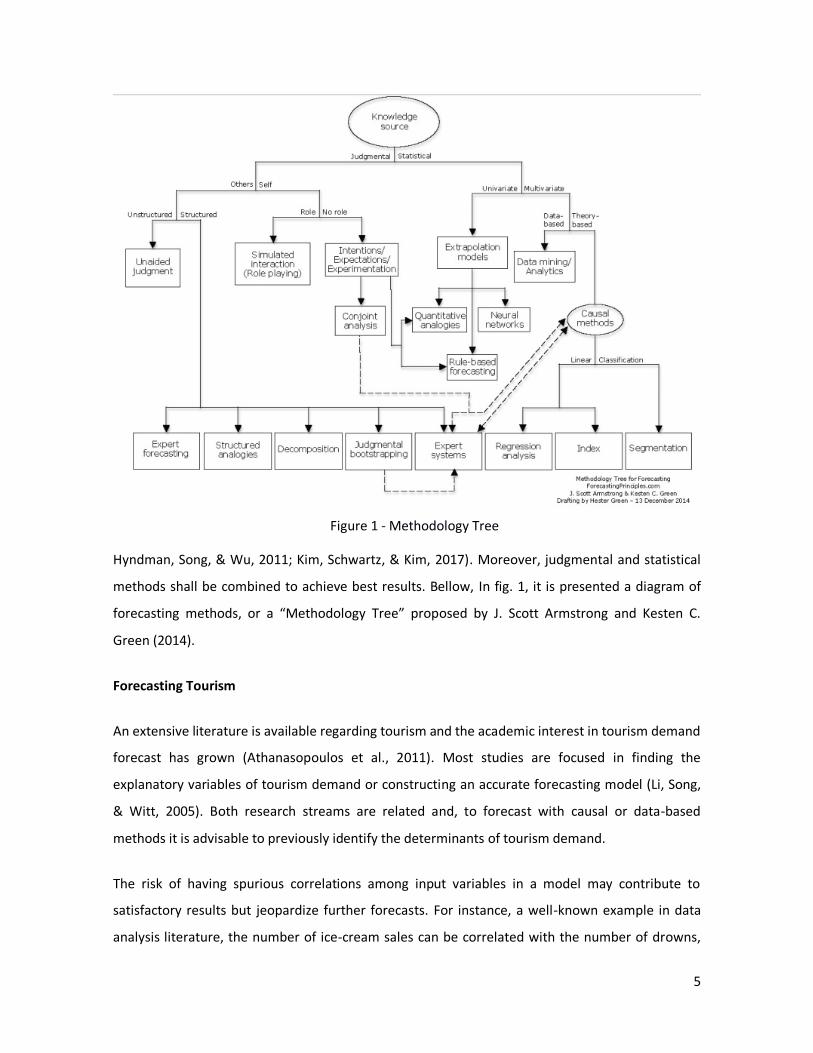
Hyndman, Song, & Wu, 2011; Kim, Schwartz, & Kim, 2017). Moreover, judgmental and statistical
methods shall be combined to achieve best results. Bellow, In fig. 1, it is presented a diagram of
forecasting methods, or a “Methodology Tree” proposed by J. Scott Armstrong and Kesten C.
Green (2014).
Forecasting Tourism
An extensive literature is available regarding tourism and the academic interest in tourism demand
forecast has grown (Athanasopoulos et al., 2011). Most studies are focused in finding the
explanatory variables of tourism demand or constructing an accurate forecasting model (Li, Song,
& Witt, 2005). Both research streams are related and, to forecast with causal or data-based
methods it is advisable to previously identify the determinants of tourism demand.
The risk of having spurious correlations among input variables in a model may contribute to
satisfactory results but jeopardize further forecasts. For instance, a well-known example in data
analysis literature, the number of ice-cream sales can be correlated with the number of drowns,
Figure 1 - Methodology Tree

6
however neither one of these two variables are the cause of each other. Both do share the same
causal variables, as the temperatures and number of visitors of that swimming place. Considering
that ice-cream sales may drop because people life’s styles evolved to more healthy habits or even
if the visitor’s profile changed to elder people who don’t eat so many ice creams as children do,
such non-sense relationship will produce biased estimates. Thus, an improved model can be
achieved to forecast drowns, if ice-cream sales are replaced by the proven causal variables
(Athanasopoulos & Hyndman, 2013)
The need for knowledge regarding tourism demand determinants was fulfilled in scientific manner
by many economists such as Gerakis (1965), Artus (1972), Bond et. Al (1977), Sunday (1978),
Archer (1980), N. Vanhove (1980), among others. They have modeled tourism demand through
econometric methods (Sheldon, 1985). The inclusion of each variable in an econometric model is
tested with statistical and economic significance tests (Armstrong, 2001). Systematic reviews
conducted by Crouch (1992, 1995, 1996) and Lim (1997) (Kim et al., 2017), have shown that the
mostly used explanatory variables are the income, price indexes, exchange rates, travel’s cost, and
demographic variables.
Researchers of tourism demand forecasting have tried to understand the underlying factors of the
available forecasting model’s accuracy performance. They have concluded that in terms of
accuracy performance there is not a model or a group of models that has proved to outstand the
others (Kim et al., 2017; Song & Li, 2008). Instead they have concluded that, besides the
forecasting method itself, the data characteristics play a significant role on every single forecasting
model and, therefore, one model cannot be applied to any dataset. The forecaster is advised to
choose the method that suits best the objectives and data characteristics:
“At the same time, despite extensive research efforts, no single model or a group of models has
been proven to be more accurate than others. At present, the process of choosing the best (i.e.,
most accurate) forecasting model(s) for a given tourism forecasting task is somewhat arbitrary,
cumber-some, and costly, with optimal results remaining unguaranteed. Therefore, the ability to
narrow down the number of forecasting methods under consideration, based on data
characteristics, would not only make the process less costly, but would also increase the likelihood
of producing more accurate predictions and, consequently, better tourism policies and managerial
decisions.”(Kim et al., 2017)

7
Regarding Song & Li (2008) review of research in the field for tourism demand forecasting done
until their study execution, the most frequently used methods for forecasting tourism demand
indicators, with a monthly data frequency are time-series methods, as broadly known. In this
group of univariate forecasting techniques, the only variable to be considered in the modeling
elaboration is the one to be forecasted. For that reason, it is less costly and simple to use. The
estimation process takes the variable’s own historical data and a disturbance term to generate
future values. There must be a correlation between observations (time lags) in order to apply
time-series methods, otherwise, no pattern in time structure is found. This type of model takes on
account three different structures or patterns in data, specifically: trend, seasonal and cyclic. A
trend is verified when a long-term (more than 1 year) decrease or increase is confirmed in data
values, not necessarily on a linear way. Seasonality is a pattern found bellow one year time-series
frequency and observation, as it can be for instance a specific day of the week, month or
trimester, it occurs in fixed period. A cyclic pattern exists when data indicates rises and falls that
happen consecutively but not in fixed period.
The satisfactory performance of time-series made them popular among forecasting researchers of
tourism demand (Song & Li, 2008), though it has a major counter back in less predictable data, as
cited by Law (2000), “the simple nature of time-series models allows them to achieve forecasting
results reasonably well (Morley, 1993; Wong, 1997). However, a fundamental limitation for time-
series forecasting models is their inability to predict changes that are not based on the past data.”.
The most frequently used technique belonging to this group of techniques are the seasonal
autoregressive integrated moving- average models (ARIMA). Lately an advanced time-series
technique has been applied in the tourism demand forecasting named the Error-Trend-Seasonal or
Exponential Smoothing (ETS) (Grose et. al, 2002 cited in Athanasopoulos et al., 2011 and Gunter &
Önder, 2015), which showed to forecast tourism demand with acceptable accuracy based on
monthly data in a recent tourism demand forecasting competition (Athanasopoulos et al., 2011).
Following the causal approach, the analyst has to identify and select the explanatory variables and
forecast the values of those independent variables so the econometric forecasting model can be
“fed”. For that reason time-series techniques still remain the starting point in a forecasting
exercise and, therefore, as cited by (Gunter & Önder, 2015), the “reliability of final forecast
outputs will depend on the quality of other variables (Chen, 2006; Uysal & Crompton, 1985, cited
in Cang, 2014)”. The basic instrument of the econometrician is regression analysis, using several

8
causal variables in additive or multiplicative functions. To forecast tourism demand, modern
econometric models have been applied, namely: the autoregressive distributed lag model (ADM);
the error correction model (ECM); the vector autoregressive model (VAR); and the time-varying
parameter model (TVP) (Allen & Fildes, 2001; Gunter & Önder, 2015). It is not clear whether the
advanced econometric models surpass the univariate or “multivariate” time-series models
probably due to misspecifications (Athanasopoulos et al., 2011). Less forecasting models have
been done with monthly data compared to time-series forecasting research (Song, Hom, & Hong
Kong SAR Gang Li, 2008). Though, businesses usually consider that knowing which influence
variables account to the forecasted variable is added value, specially under certain business or
economic circumstances (Allen & Fildes, 2001; Kordon & Rey, 2012) and, for volatile tourism
demand destinations or in moments of foreseen changes it is better take a safe option and rely in
causal or combined forecasting approaches. An example of this, was the inability of univariate
forecasts to show the impact in businesses of the imminent 2008/2009 recession where, the use
of multivariate explanatory variables framework, would have given in advance some evidence of
the changes in demand (Kordon & Rey, 2012).
The data-base or data driven forecasting stream, belongs to the emerging forecasting techniques
referenced by Song & Li (2008) review. Nowadays, those techniques are under the interdisciplinary
subject, so called “Data Mining”. It came from a from a state a lack information despite of data
abundance, due to a data “explosion” that came with computing power, internet and business
intelligence systems, the need for finding useful information in large data repositories was
satisfied by a combination of hardware technology, algorithms, statistics and machine learning.
Computers allowed analysts to run many types of procedures that start with nearly a value or set
of values and produces another value or a set of values, known as output. An algorithm transforms
de initial data, throughout a sequence of steps or rules into a nominal or numerical result, and so
it models the input and output relationship. As for statistics, “a statistical model is a set of
mathematical functions that describe the behavior of the objects in a target class in terms of
random variables and their associated probability distributions” (Kamber et al., 2012). Machine
learning definition is almost philosophical but can be seen as the ability of a computer program
(algorithm) to capture patterns in data and produce information that can be a classification or
prediction exercise from a supervised or unsupervised learning. The first type of learning,
supervision is held by a labeled input, which may be nominal or numerical. The second type of

9
learning is the opposite, usually a clustering is the main technique applied in the dataset order to
distinguish the composing elements, thus is more related to a classification exercise. On the other
hand, supervised learning can be used to make predictions or, estimate future values, in the form
of classification (discrete variables) or regression (when we have continuous variables) outputs.
As mentioned before, traditional methods like time-series or econometric are quite suitable for
data characterized by specific behavior like, trend, seasonality and cyclicality. On the contrary,
artificial intelligence methods like the Artificial Neural Networks (ANNs) algorithm discards
statically assumptions about the data to be applied. These techniques can deal with imperfect and
irregular data or nonlinear behavior, and late studies are demonstrating that its accuracy is
satisfactory (Claveria, Monte, & Torra, 2014; Constantino, Fernandes, & Teixeira, 2016; Teixeira &
Fernandes, 2012). Although some academic findings point out that there is not a one-fit-all
forecast technique for all source markets and forecast horizons, the advantage of using machine
learning algorithms is clear under the premise that the system may become chaotic, as stated by
Baggio, R., & Sainaghi, R. (2016).
Machine Learning Algorithms
Decision Tree and Random Forests
A decision tree method belongs to the supervised machine learning algorithms. The input
variables are related to a pre-defined target variable, which can be either categorical or
continuous meaning that the decision tree model can be a Classification Tree or a Regression Tree,
respectively.
The method consists in dividing up a population or sample data (root node) into two or more
smaller subsets of similar tuples (leaf nodes) until a class label is reached (terminal node), on the
most significant differentiator in input variables (internal nodes).
In general, a decision tree algorithm works from top to down, i.e., it begins by splitting in the most
homogeneous attribute or input variable (root node) and keeps dividing the into a Leaf or a

10
Terminal node, a purer node (more homogeneous) than the previous node based in decision rules
or constraints with respect to a target variable. This is so called divide-and-conquer or greedy
approach, which was developed by J. Ross Quinlan, a researcher in machine learning, from the
University of Sydney between de 70’s and early 80’s. His work comprises the ID3 algorithm, the
first successful one, known for the use of information gain criterion and, the C4.5 algorithm, the
successor of ID3 and benchmark for new algorithms. C4.5 showed a series of improvements in
dealing with numeric attributes, noisy data and in rules generation. C5 is another version of C4.5
with more features that make the process of tree grow faster, efficient (less memory needed), and
an improved purity measure.
CART is another decision tree algorithm that stands for Classification and Regression Tree,
published by L. Breiman, J. Friedman, R. Olshen, and C. Stone (1984) in parallel with invention of
ID3. The collection of decision trees has grown since then, and nowadays it is possible to compute
many decision trees in one algorithm (Random Forest) that selects the best ones and averages the
outputs, one of the machine learning ensemble methods.
11
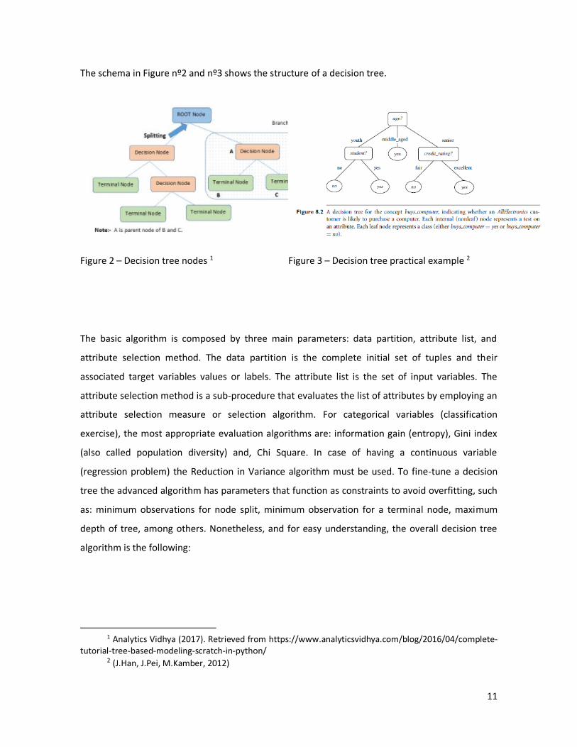
The schema in Figure nº2 and nº3 shows the structure of a decision tree.
Figure 2 – Decision tree nodes 1
Figure 3 – Decision tree practical example 2
The basic algorithm is composed by three main parameters: data partition, attribute list, and
attribute selection method. The data partition is the complete initial set of tuples and their
associated target variables values or labels. The attribute list is the set of input variables. The
attribute selection method is a sub-procedure that evaluates the list of attributes by employing an
attribute selection measure or selection algorithm. For categorical variables (classification
exercise), the most appropriate evaluation algorithms are: information gain (entropy), Gini index
(also called population diversity) and, Chi Square. In case of having a continuous variable
(regression problem) the Reduction in Variance algorithm must be used. To fine-tune a decision
tree the advanced algorithm has parameters that function as constraints to avoid overfitting, such
as: minimum observations for node split, minimum observation for a terminal node, maximum
depth of tree, among others. Nonetheless, and for easy understanding, the overall decision tree
algorithm is the following:
1 Analytics Vidhya (2017). Retrieved from https://www.analyticsvidhya.com/blog/2016/04/complete-
tutorial-tree-based-modeling-scratch-in-python/ 2 (J.Han, J.Pei, M.Kamber, 2012)

12
Inputs: D (data partition); attribute_list; Attribute_selection_method
(1) create a node N;
(2) if tuples in D are all of the same class, C, then
(3) return N as a leaf node labeled with the class C;
(4) if attribute list is empty then
(5) return N as a leaf node labeled with the majority class in D; // majority voting
(6) apply Attribute selection method(D, attribute list) to find the “best” splitting criterion;
(7) label node N with splitting criterion;
(8) if splitting attribute is discrete-valued and
multiway splits allowed then // not restricted to binary trees
(9) attribute list attribute list � splitting attribute; // remove splitting attribute
(10) for each outcome j of splitting criterion
// partition the tuples and grow subtrees for each partition
(11) let Dj be the set of data tuples in D satisfying outcome j; // a partition
(12) if Dj is empty then
(13) attach a leaf labeled with the majority class in D to node N;
(14) else attach the node returned by Generate decision tree(Dj , attribute list) to node N;
endfor
(15) return N;

13
Decision Trees attribute selection methods:
Information gain after partitioning based on attribute
A
The average amount of information needed to identify
a class, know as the entropy of D.
The expected information required to arrive to an
exact classification based on attribute A.
The reduction of impurity that would be achieved by a
binary split of attribute A.
Impurity of data partition.
Impurity of attribute A.
High chi-square test score means that the proposed
attribute splits the set into subsets, with significantly
different distributions, hence the splitting is not based
merely on chance.
Δ(A) = Var(D) – VarA(D) The reduction of variance in data partition through the
split of attribute A, augmenting the homogeneity of
the subset.

14
Artificial Neural Network (ANN)
Inspired on a work of a psychologist and neurobiologist that constructed a logical model of the
functioning of biological neurons (between the 1930 and 1940), before the existence of digital
computers, computer scientists in the 50’s developed neural network algorithms. However, due to
low computer power and theoretical deficiencies, it was only reliable to use ANNs after the
improvement of computer performance in the 80’s and invention of the backpropagation
algorithm in 1983 by John Hopfield, which bypassed the theoretical drawbacks and catapulted
ANN, more precisely, the Multilayer feed-forward network, from the researcher’s domain into the
commercial world.
In the basis of ANN is the perceptron learning rule (simple neural network), an algorithm created
by Rosenblatt in 1958, that constructs linear combination of weighted inputs and a bias coefficient
through an iterative correction process aiming a target value or class, resulting in a hyperplane,
the “grandfather” of neural networks. When an instance or tuple is presented to perceptron, the
input values are submitted to the previously defined linear function and an estimate is produced.
Such basic algorithm can only deal with linearly separable data for a classification or regression
problem, as proved by Minsky and Papert (1969) (Kamber et al., 2012). For the nonlinear
separation, it is necessary to have more than one perceptron or neuron, thus a multilayer
perceptron may be applied, a commonly used class of multilayer feed-forward network.
A Multilayer Feed-Forward network is made of an input layer, the measured attributes, one or
more hidden layers, which may have one or more interconnected neurons (perceptrons) and, the
output layer where results are returned (Figure 4). The flow of data, through the sequence of the
previously described elements of such ANN, is called Forward Propagation.

15
Figure 4 – Multi-layer feedforward neural network3
The usefulness of a ANN comes with the ability of modeling nonlinear behavior of data. Nonlinear
behavior may be encountered when slight changes on the input result in profound changes on the
output or when major changes in the input produce insignificant impact on the result. Such
feature is achieved by applying a non-linear transfer function to the sum of the combined weights
(activation value) and inputs, known as the activation function. The most known transfer functions
to run a non-linear transformation are the sigmoidal (Logistic function), hyperbolic tangent (TanH)
and Gaussian.
Sigmoidal TanH Gaussian
The backward flow is known as Backward Propagation and it is where the backpropagation
algorithm takes place by computing the error values for each output node with respect to the
target value and the error for the nodes in hidden layers with respect to the next hidden layer.
After that, it finds the error correction values for the weights and biases (used in each combination
3 (J.Han, J.Pei, M.Kamber, 2012)

16
function), using a mathematical method, the Gradient Descent, which allows to find the global
optimal combination of weights that will minimize the mean square error. And last, it updates the
weights and biases. The process of forward and backward propagation repeat until one of the
stopping criteria is met, such as: the error correction values are bellow a user-defined threshold;
the defined accuracy was reached; or the specified number of epochs (iterations) was completely
spent.
4
4 (J.Han, J.Pei, M.Kamber, 2012)

17
Support Vector Regression
The Support Vector Regression machine learning method was derived from the support vector
machine algorithm (SVM) created only to serve classification problems. Nevertheless, it shares
many of the same principles of SVM. Basically, what SVR does is to find a regression function that
fits well the training instances by minimizing the prediction error, this error is user defined and
forms tube around the regression function, discarding all the data points that are outside the
margin. Besides minimizing the error, the algorithm maximizes the flatness of the regression
function for generalization purpose. The larger the tube (bigger error deviation) the flatter the
function. However, if encloses most of the data points, the model will be meaningless. Thus, it is
necessary to achieve a tradeoff between the error minimization and the flatness of the function.
Any SVR exercise has the following solution:
Where w are the weights that most flatten the function, constrained by the user specified error
deviation threshold ( ).
The linear function of SVR can be written as:
For a non-linear problem, the inner product between the support vectors and the attribute
instances can be substituted by a kernel function, polynomial or gaussian radial basis, that will
transform the that to a higher dimensional feature space to allow a linear fit of the training data
(Figure 5).

18
5
5 Sayad, S. (2017). An Introduction to Data Science. Retrived from http://www.saedsayad.com/data_mining_map.htm
Figure 5 – Kernel’s “magic”
19
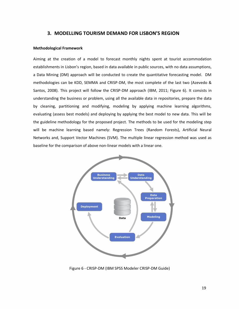
3. MODELLING TOURISM DEMAND FOR LISBON’S REGION
Methodological Framework
Aiming at the creation of a model to forecast monthly nights spent at tourist accommodation
establishments in Lisbon’s region, based in data available in public sources, with no data assumptions,
a Data Mining (DM) approach will be conducted to create the quantitative forecasting model. DM
methodologies can be KDD, SEMMA and CRISP-DM, the most complete of the last two (Azevedo &
Santos, 2008). This project will follow the CRISP-DM approach (IBM, 2011; Figure 6). It consists in
understanding the business or problem, using all the available data in repositories, prepare the data
by cleaning, partitioning and modifying, modeling by applying machine learning algorithms,
evaluating (assess best models) and deploying by applying the best model to new data. This will be
the guideline methodology for the proposed project. The methods to be used for the modeling step
will be machine learning based namely: Regression Trees (Random Forests), Artificial Neural
Networks and, Support Vector Machines (SVM). The multiple linear regression method was used as
baseline for the comparison of above non-linear models with a linear one.
Figure 6 - CRISP-DM (IBM SPSS Modeler CRISP-DM Guide)

20
This project framework was inspired in light of previous forecasting exercises, besides the DM
approach, such as those studies published by (Cankurt & Subai, 2015.; Constantino et al., 2016)
where the forecasting of monthly nights spent at tourist accommodation establishments for a
specific localization using machine learning algorithms was attempted. Here, due to practical
reasons, the chosen tourism source market was the UK, which is one of the top five main tourist’s
source markets for the region of Lisbon and, thus considered meaningful to the region’s economy.
As for the machine learning methods, in previous forecasting exercises, the most used is the
artificial neural network. Nonetheless, this project rational is to use all the available resources to
achieve the most accurate multivariate DM model.
The practical stages of the current project can be structured into:
1. Data
1.1 data collection
1.2. data preparation
1.3. Data Partitioning
2. Experiments
2.1. Modeling and Attribute selection
2.2. Model’s evaluation and selection
3. Scenario Forecasting.
The Data Mining workbench software used in the current project for modeling and prediction was
Weka 3.8, an open source java software developed by the University of Waikato of New Zealand
(available for download in: https://www.cs.waikato.ac.nz/ml/weka/downloading.html)

21
Data
A preliminary search of explanatory variables for tourism demand in the literature has been done.
Macroeconomic variables, such as GDP, income and consumer price index are examples of
reviewed explanatory variables for tourism demand (Daniel & Ramos, 2002). Those variables are
available in internet data sources, with a monthly frequency, therefore, they were included in the
dataset, and the rest were not. Rarely used variables, such as google trends, currency exchange
rates and stock market index were also included. To guarantee the reliability of data and, that any
person can replicate the model, the data sources for the time-series variables used in this project
were from official entities and strictly the ones available to everyone in the internet, namely:
Instituto Nacional de Estatística (INE) - https://www.ine.pt;
o nights spent at tourist accommodation establishments in Lisbon’s region
o Number of tourists at accommodation establishments in Lisbon’s region
UK Office for National Statistics (ONS) - https://www.ons.gov.uk/
o Consumer Price Index (CPI)
o Retail Price Index (RPI) for Travel and Air Passangers
Eurostat (European Commission) - http://ec.europa.eu/eurostat;
o Financial account - monthly data
o Consumers - monthly data
o Harmonised indices - monthly data
o Harmonised unemployment rates (%) - monthly data
o Interest rates - monthly data
o Nights spent at tourist accommodation establishments - monthly data
Investing.com - https://www.investing.com/
o GBP/EUR Exchange Rate Historical Data
Google Trends - https://trends.google.pt/

22
o Search words “#” by country of origin “()”: #Lisbon (England); #Lisboa (England);
#cascais (England); #oeiras (England); #sintra (England); #Lisbon (Northern
Ireland); #Lisboa (Northern Ireland); #cascais (Northern Ireland); #sintra (Northern
Ireland); #Lisbon (Scotland); #Lisboa (Scotland); #cascais (Scotland); #oeiras
(Scotland); #sintra (Scotland); #Lisbon (Wales); #Lisboa (Wales); #cascais (Wales);
#sintra (Wales)
The data was extracted from Eurostat in bulk download and, from the other websites through
export feature, in various file formats (“.tsv”, “.txt”, “.csv”, “.xlsx”), which were assembled in
Microsoft Access with some VBA coding for file and data manipulation purposes. The dataset table
had 1.097 variables mainly because of Eurostat data, that has most of the variables under this
study and various demographic segmentation for each variable (country, age, gender) and data
scales (percentage, ratio, thousands).
The SQL table was then exported to Excel format. The variables were then filtered to have a period
ranging from January’s 2004 until December’s 2015, a total of 144 months. Since in Data Mining
approach there are no data assumptions and due to the robustness of the modern machine
learning algorithms, transformations to data or outlier’s treatment were not applied. Fortunately,
because of systematic data management of those information suppliers (INE, Eurostat and the
others), the cleaning of data was resumed to some characters deleting in order to have only
numbers. There were no missing values to deal with.
Accordingly to IMPACTUR report (Perna, Custódio, & Gouveia, 2009) and, has seen in Figure nº7,
the target variable has a seasonal component, therefore a new variable based on the target
variable T-12 lags was added to the original dataset and named as
“#lagged_12m_ine_dormidas_Lisboa_Reino Unido”. As previously mentioned, forecasting studies
state that a T-1 lagged target variable is correlated to the target variable and since it improves the
models performance it was also added to the initial dataset.
For ordering purpose, the variable “#Nr_Mes” was added with a range of 13 to 144, corresponding
to 132 months from the year 2005 to 2015. The instances 1 to 12 of the year 2004 were excluded
since for the 12-lagged target variable there were no available data from 2003, and also because
the year of 2004 had an special event, the European Football Championship that led many

23
occasional tourist to come to Lisbon. The variable “#Mes” was created and included so the
monthly periodicity could be considered in modeling.
Five more variables ended in “_var” were computed from the monthly variation of the variables
“#ine_hospedes_Lisboa_Reino Unido”, “#GBP/EUR”, “#RPI_Travel_UK”, “#CPI_UK”, “#FTSE_100”
were created during the first experiment process as they seemed to contribute to the models
accuracy. In total, the full dataset (“TourismDataset”) has 1.105 input attributes plus 1 target
variable with 132 instances / months regarding the period of 2005 – 2015.
Figure 7 – Nights spent by UK residents at tourism establishments in Lisbon’s region (2004 – 2015)
Experiments
As shown in the CRISP-DM methodology schema (Figure nº6), a cyclic process of experimentation
of different machine learning algorithms (modeling) and combinations of attributes (data
preparation) is part of the learning process and hereby mentioned as “experiments”, which is
Weka’s software terminology. In this report it is described 3 experiments executed with a data
partition of 91% for training (120 instances) and 9% for testing (12 instances) to capture data
behavior of most recent years and, with the same set of algorithms applied to 3 different datasets.
Between the experiments, a progressive attribute selection was performed to reduce non-relevant
variables and to augment the models accuracy, which is further explained.

24
Modeling and Attribute selection
To compare the models generated by the machine learning algorithms the baseline model was the
Linear Regression. The set of machine learning algorithms was restricted to a few parameter
variation to avoid time consumption and minimize the insertion of multiple heuristics.
List of applied algorithms and respective parameter configuration:
1 Multiple Linear Regression (MLR)
Weka reference: weka.classifiers.functions.LinearRegression
Weka parameter configuration: S 1 -R 1.0E-8 -num-decimal-places 4
A Linear Regression with no prior testing of assumptions, no attribute selection, no prior
check of capabilites (data type, missing values).
2 Random Forests
Weka reference: weka.classifiers.trees.RandomForest
Weka parameter configuration:
- P 100 -I 100 -num-slots 1 -K 0 -M 1.0 -V 0.001 -S 1
- P 100 -attribute-importance -I 100 -num-slots 1 -K 0 -M 1.0 -V 0.001 -S 1
The default algorithm to construct a forest of decision trees in weka has 100% of bag size
(the whole training dataset)(P), 100 iterations (I), 1 ensemble exectution (thread) (num
slots), zero randomly chosen attributes (K), 1 as minimum of instances per leaf (M), 0,001
minmum of variance per split (attribute spliter)(V), 1 seed (S). The second algorithm has a
aditional feature that computes and outputs attribute importance, by the mean impurity
decrease method (attribute-importance = TRUE)
3 Artificial Neural Networks (Multi Layer Percepetron – MPL)
Weka reference: weka.classifiers.functions.MultilayerPerceptron
Weka parameter configurations:
- L 0.3 -M 0.2 -N 500 -V 0 -S 0 -E 20 -H 2

25
- L 0.3 -M 0.2 -N 500 -V 0 -S 0 -E 20 -H 3
- L 0.3 -M 0.2 -N 500 -V 0 -S 0 -E 20 -H 4
Default ANN learning algorithm in Weka has a learning rate of 0.3 (L), momentum of 0.2
(M), 500 epochs (N), 0 seeds, validation threshold of 20 (E). The 3 neural network models
differ in the number of hidden layers (2, 3 and 4) (H), which intensify the non-linear
relationship among perceptron functions in the model.
Support Vector Machines (SMOReg)
Weka reference: weka.classifiers.functions.SMOreg
- C 0.5 -N 0 -I \"weka.classifiers.functions.supportVector.RegSMOImproved -T
0.001 -V -P 1.0E-12 -L 0.001 -W 1\" -K
\"weka.classifiers.functions.supportVector.PolyKernel -E 1.0 -C 250007\"
- C 1.0 -N 0 -I \"weka.classifiers.functions.supportVector.RegSMOImproved -T
0.001 -V -P 1.0E-12 -L 0.001 -W 1\" -K
\"weka.classifiers.functions.supportVector.PolyKernel -E 1.0 -C 250007\"
- C 1.5 -N 0 -I \"weka.classifiers.functions.supportVector.RegSMOImproved -T
0.001 -V -P 1.0E-12 -L 0.001 -W 1\" -K
\"weka.classifiers.functions.supportVector.PolyKernel -E 1.0 -C 250007\"
- C 2.0 -N 0 -I \"weka.classifiers.functions.supportVector.RegSMOImproved -T
0.001 -V -P 1.0E-12 -L 0.001 -W 1\" -K
\"weka.classifiers.functions.supportVector.PolyKernel -E 1.0 -C 250007\"
The SMOReg is the support vector regression algorithm in Weka, by default it uses the
RegOptimizer to automatically learn most of the algorithm’s parameters, in this case the
improved version was chosen to better performance (I). The C is the complexity coefficient
responsible for the level of fitting and it where the four version are distinguished. The rest
of the parameter are by default, N parameter is set to normalize the variables so they
have the same scale, 0,001 for the stopping criterion (T), by default the variant of the
algorithm is 1 of 2, the epsilon is the error deviation threshold and is set to 1 (P), the
epsilon for the loss-function is also set to 1 (L), 1 random seed (W), Polykernel is the
nonlinear function used In most of support vector machine algorithms.

26
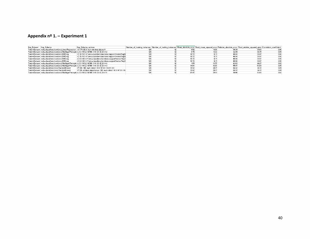
For Experiment number 1 (Exp.1) the dataset used was the full attribute dataset
“TourismDataset.arff” and with the already described data partition and group of ML algorithms.
The results are displayed in Appendix nº 1. In this experiment, the number of heuristics is the
minimum has possible, it is a start point to compare further experiments with selected attributes
to improve model’s accuracy.
After Exp.1 and, before a new learning process, to eliminate irrelevant variables and at the same
time find the attribute interrelationships and bypass linear relationship selection, the algorithm
used for attribute selection was the Relief (Arauzo-Azofra, Benítez, & Castro, 1994). In Weka it is
named as “ReliefFAttributeEval” (evaluator algorithm) and, in this project it was combined with a
search algorithm called “Ranker”. Both algorithms were used with the Weka’s default parameter
configuration. Before applying the Relief attribute selector , to find out the number of attributes to
use has threshold in the Ranker’s algorithm, the correlation based evaluator algorithm
“CfsSubsetEval” combined with the search algorithm “BestFirst” was used. The output informed
19 relevant variables, which were not considered in the next experiment due to the linear
constraints (Appendix nº 2). The attribute selection with Relief restricted to 19 variables was
performed using the TourismDataset (full details in Appendix nº 3).
For Experiment number 2 (Exp.2) the dataset used was the full attribute dataset
“TourismDataset.arff” and the dataset “dataset_19_Relief.arff” (19 selected variables) with the
already described data partition and group of ML algorithms (full details in Appendix nº4).
From Exp.2, another attribute selection was done with the best model (Appendix nº6) but, this
time, with manual selection of variables to verify the impact on the model’s accuracy. It was found
that without the variable “#ine_hospedes_Lisboa_Reino Unido” (number of tourism guests) the
model’s accuracy was improved (full details in Appendix nº7). Results of a correlation test
(Spearman) applied to the selected variables show strong correlations that can be linear or non-
linear (full details in Appendix nº 8). Hence, the next dataset was created with 18 variables and
named has “dataset_18_Relief_no_hospedes.arff”.
For the last experiment (Exp.3), the dataset used was the full attribute dataset
“TourismDataset.arff”, the “dataset_19_Relief.arff” (19 selected variables) and the

27
“dataset_18_Relief_no_hospedes.arff” (18 selected variables), with the already described data
partition and group of ML algorithms (full details in Appendix nº 9).
The experiments output comprises model’s evaluation metrics and algorithms efficiency (not
analyzed in this work). In the following section, the evaluation of the models in each experiment is
explained. The stages of modeling and evaluation are in permanent articulation, here for
pedagogical purposes they are described separately.
Models Evaluation and Selection
In each single experiment the model’s evaluation metrics analyzed were the mean absolute error
(MAE) and the root mean squared error (RMSE). Additionally, the correlation coefficient (R²) was
used to know how well the predicted values change with the actual values.
The mean absolute error is the (MAE) average of the module of absolute differences between the
predicted and the actual values (ei) or, the typical error deviation. It is possible to check how close
the average of the predicted values are close to the average of the target values from the test set
and, therefore, it informs the models’ bias.
To know how accurate the model is, the root mean absolute error (RMSE) is used. Since the errors
are squared before being averaged, it gives relatively more weight to larger error differences.
Therefore, it informs the impact of outliers in the model’s bias and provides a measure of
precision.

28
4. RESULTS AND DISCUSSION
Analyzing the test results of Exp.1, the Linear Regression outstand the rest of the algorithms in
RMSE (and R²), followed very closely by the MLP H2 which had the best MAE of all (summary in
table nº 1, full details in Appendix nº 1). Outlier values seem to have similar impact in MLR and
MLP, since RMSE is almost equal on both models. The MLR correlation coefficient is quite high,
which indicate a relative good fit of the model’s test predictions but, the bias measure (MAE) is
much lower on MLP, which points toward a better accuracy. MLP showed to have the best
performance in modeling an ordered dataset of a high dimension, which may indicate a
“presence” of non-linearity relationship. Additionally, has explained before, MLR model cannot be
considered reliable for estimation since its assumption were not tested. Nevertheless, MLR works
as a benchmark for the experiments.
Dataset Algorithm Parameter's options MAE RMSE R^2
TurismDataset MLR -S 1 -R 1.0E-8 -num-decimal-places 4 9.522 11.060 0.964
TurismDataset MLP -L 0.3 -M 0.2 -N 500 -V 0 -S 0 -E 20 -H 2 8.704 11.325 0.939
TurismDataset SMOreg -C 1.0 10.724 12.106 0.965
Table 1 – Exp.1
After the first attribute selection, Exp.2 was conducted to assess the best trade-off between full
and attribute selected datasets and algorithms. In Exp.2 (table nº 2), it is evident the superior
performance with the attribute selected dataset (“dataset_19_Relief.arff”) and the support vector
regression algorithm (SMOReg C 2.0) in all evaluation metrics (full details in Appendix nº 4).
SMOReg C2.0 was then used for the second attribute selection evaluation, were it was achieved a
reduction of 3.169 on MAE and of 3.114 on RMSE (see table nº 3 and, full details in Appendix nº 6
and nº7).

29
Table 2 – Exp. 2
Evaluation measures dataset_19_Relief (A) dataset_18_Relief_no_hospedes (B) Diff. (B-A)
Correlation coefficient 0.9539 0.9422 -0.012
Mean absolute error 9.255 6.0861 -3.169
Root mean squared error 10.3873 7.2737 -3.114
Relative absolute error 35.08% 23.07% -12%
Root relative squared error 33.44% 23.41% -10%
Total Number of Instances 12 12 0
Table 3 - Test results of SMORef C 2.0 model on dataset_19_Relief (with and without variable
"hospedes")
The last experiment (Exp. 3) was run to assess the best model with the last dataset
“dataset_18_Relief_no_hospedes.arff” (18 selected variables). Analyzing the results of Exp. 3 in
table nº 4 (full details in Appendix nº 9), the SMOReg was still the best model achieved after the
attribute selection, especially in the RMSE metric, followed by the MLR and MLP (H2). However,
the version SMOReg with a C of 1.0 outperformed the version with a C 2.0 by a difference of less
0.06 on MAE. Therefore, it is the selected model for the forecasting exercise (bellow is the model’s
results summary and a chart showing the test prediction outputs, full details in Appendix nº 10).
Dataset Algorithm Parameter's options MAE RMSE R^2
dataset_19_Relief SMOreg -C 2.0 9.255 10.387 0.954
dataset_19_Relief SMOreg -C 1.5 9.597 10.700 0.953
dataset_19_Relief SMOreg -C 0.5 9.635 10.858 0.950
dataset_19_Relief SMOreg -C 1.0 9.767 10.934 0.952
TurismDataset MLR -S 1 -R 1.0E-8 -num-decimal-places 4 9.522 11.060 0.964
TurismDataset MLP -L 0.3 -M 0.2 -N 500 -V 0 -S 0 -E 20 -H 2 8.704 11.325 0.939
dataset_19_Relief MLR -S 1 -R 1.0E-8 -num-decimal-places 4 10.243 11.546 0.943
dataset_19_Relief MLP -L 0.3 -M 0.2 -N 500 -V 0 -S 0 -E 20 -H 4 10.574 11.829 0.967
TurismDataset SMOreg -C 1.0 10.724 12.106 0.965

30
Dataset Algorithm Parameter's options MAE RMSE R^2
dataset_18_Relief_no_hospedes SMOreg - C 1.0 6.024 7.234 0.943
dataset_18_Relief_no_hospedes SMOreg - C 1.5 6.041 7.259 0.942
dataset_18_Relief_no_hospedes SMOreg - C 2.0 6.086 7.274 0.942
dataset_18_Relief_no_hospedes SMOreg - C 0.5 6.460 7.716 0.939
dataset_18_Relief_no_hospedes LinearRegression - S 1 -R 1.0E-8 -num-decimal-places 4 6.132 8.542 0.918
dataset_19_Relief SMOreg - C 2.0 9.255 10.387 0.954
dataset_19_Relief SMOreg - C 1.5 9.597 10.700 0.953
dataset_19_Relief SMOreg - C 0.5 9.635 10.858 0.950
dataset_19_Relief SMOreg - C 1.0 9.767 10.934 0.952
Table 4 – Exp.3
=== Summary ===
Correlation coefficient 0.9425
Mean absolute error 6.0237
Root mean squared error 7.2338
Relative absolute error 0.2283
Root relative squared error 0.2329
Total Number of Instances 12
Table 5 - Summary of the SMOReg – C1.0 modelling results

31
Figure 8 - Test predictions with SMOReg C1.0 (Exp.3)
In reference to stochastic forecasting exercises of IMPACTUR, a MAE percentage below 10% is
considered insufficient. The evaluation metrics are not promising of a high level of forecasting
accuracy for the selected model, with a relative absolute error (MAE in percentage) of 22.83% and
a Root Relative Absolute Error (RMSE in percentage) of 23.28%. Nonetheless and, since the
model’s generalization capability was roughly tested, due to small number of dataset instances,
the forecast exercise shall proceed with the best achieved model.
Scenario Forecasting
Since the data mining model predicts through interpolation, it is necessary to have accurate
observations of explanatory variables in a future period and, in the absence of official data it
would be necessary to undertake several studies for all the input variables to find reasonable
estimates for them, which is not viable for this project. In order to forecast the target variable for
a 12 month horizon (2016 year), using real data, three future plausible scenarios defined as
unfavorable (Scenario 1), moderated (Scenario 2), and favorable (Scenario 3). To obtain the input
variables, the averages of the attribute values were calculated in the following way for each
scenario.

32
Scenario 1 (unfavorable) – for each independent variable, it was computed the average of each
month of the 2005-2009 period (5 years prior to the financial crises);
Scenario 2 (moderate) – for each independent variable, it was computed the average of each
month of the 2011-2015 period (5 years after financial crises), the year 2010 was excluded has it is
the inflexion point of the dependent variable;
Scenario 3 (favorable) – for each independent variable, the average of each month of the 2014-
2015 (2 years of great growth of the dependent variable);
For the 12m-lagged target variable “#lagged_12m_ine_dormidas_Lisboa_Reino Unido” the real
values off the year 2015 were used and, for the 1m lagged variable
“#lagged_1m_ine_dormidas_Lisboa_Reino Unido” the value of the last instance of the target
variable (january’s 2015) was used to begin the model’s predictions. Every time an estimate was
computed for each month, it was used as input value for the attribute
“#lagged_1m_ine_dormidas_Lisboa_Reino Unido”. The results are shown in the graphical
representation (Figure nº9) and full details in Appendix nº 11, 12 and 13. Since the variable under
this study was published in INE’s 2016 Tourism Statistics without the month frequency, the
predicted total value was compared to the total actual value in table nº 6. The scenario’s estimates
with highest forecasting accuracy were achieved in scenario 3, which is not surprising because this
scenario used the most recent data.
Figure 9 – Scenario Forecast h = 12m (year 2016)

33
Figure 10 - Nights spent by UK residents at tourism establishments in Lisbon’s region (2004 –
20166)
Scenarios Predicted Values (2016)* Actual Values (2016)* Absolute Error (%)**
Scenario 1 778.6 845.6 7.92
Scenario 2 818.6 845.6 3.19
Scenario 3 851.1 845.6 0.65
Table 6 – Forecast error evaluation (*Total in thousands)
**Absolute Percentage Error formula:
6 Estimated values for 12 month period of 2016’s year

34
5. CONCLUSIONS
The objectives of the current project work were enhance the available public sources of tourism
forecast information and contribute to the tourism stakeholder’s strategy in Portugal. More
specifically, to develop a multivariate model to forecast international tourism demand through a
Data Mining approach. The forecasted variable was the nights spent at tourist accommodation
establishments in Lisbon’s region, one of the country’s main foreign tourist destinations. The
model development was constrained to publicly available data and machine learning methods.
Instead of revealing a best forecasting method or model, as most of previous research sought to,
the current project aimed at building the most accurate multivariate forecasting model, based on
a database with minimum data assumptions. The objectives were achieved, as the selected model
(SMOReg) was successful in generalization capability, in resemblance to a similar case study in
Turkey. And, despite of having a high relative absolute error and Root Relative Absolute Error in
the test phase, the model produced quite accurate forecasts, especially in scenario 3.
To improve the accuracy in the modelling stage, more qualitative and quantitative variables could
be introduced. Such explanatory variables might be the number of marketing campaigns,
investments, travel’s price, and even a sentiment analysis in social and online media. This
information must be obtained from tourism stakeholders. Moreover, it would be crucial to fine
tune the machine learning model’s parameters in several trials.
As it was observed, both the European economy and the interest of UK residents in Lisbon’s
Region kept growing slightly in 2016. The “matching” of the total forecasted values of favorable
scenario with the total actual values of nights spent at tourist accommodation establishments in
Lisbon’s region in 2016, provides some evidence of the reliability of the proposed forecasting
model.
In summary, if institutions and decision makers have information regarding the evolution of the
explanatory variables used in this model, the impact on Lisbon’s tourism demand can be assessed,
even in case of an emerging recession.

35
REFERENCES
Armstrong, J. Scott (2001). Principles of Forecasting: A Handbook for Researchers and
Practitioners. Norwell, MA(2001)
Armstrong, J. Scott and Green, Kesten C. (2014). Methodology Tree for Forecasting. Retrieved
from http://forecastingprinciples.com/files/methodology-tree_2014.pdf
Athanasopoulos, G., Hyndman, R. J., Song, H., & Wu, D. C. (2011). The tourism forecasting
competition. International Journal of Forecasting, 27(3), 822–844.
https://doi.org/10.1016/j.ijforecast.2010.04.009
Azevedo, A., & Santos, M. F. (2008). KDD, SEMMA and CRISP-DM: a parallel overview. IADIS
European Conference Data Mining, (January), 182–185. Retrieved from
http://recipp.ipp.pt/handle/10400.22/136
Baggio, R., & Sainaghi, R. (2016). Mapping time series into networks as a tool to assess the
complex dynamics of tourism systems. Tourism Management, 54, 23–33.
https://doi.org/10.1016/j.tourman.2015.10.008
Cang, S. (2014). A Comparative Analysis of Three Types of Tourism Demand Forecasting Models :
Individual , Linear Combination and Non-linear Combination, 607(May 2013), 596–607.
https://doi.org/10.1002/jtr
Cankurt, S., & Subai, A. (2015). Tourism demand modelling and forecasting using data mining
techniques in multivariate time series: a case study in Turkey. https://doi.org/10.3906/elk-
1311-134
Chase, C. W., & Jr. (2013). Demand-Driven Forecasting: A Structured Approach to Forecasting, 384.
Retrieved from https://books.google.com/books?hl=en&lr=&id=iVIbAAAAQBAJ&pgis=1
Chatziantoniou, I., Degiannakis, S., Eeckels, B., & Filis, G. (2016). Forecasting tourist arrivals using
origin country macroeconomics. https://doi.org/10.1080/00036846.2015.1125434
Claveria, O., Monte, E., & Torra, S. (2014). “ A multivariate neural network approach to tourism
demand forecasting .”

36
Claveria, O., Monte, E., & Torra, S. (2016). Applied Economics Letters Combination forecasts of
tourism demand with machine learning models Combination forecasts of tourism demand
with machine learning models. https://doi.org/10.1080/13504851.2015.1078441
Constantino, H. A., Fernandes, P. O., & Teixeira, J. P. (2016). Tourism demand modelling and
forecasting with artificial neural network models: The Mozambique case study. Tékhne.
https://doi.org/10.1016/j.tekhne.2016.04.006
Cunha, L. & Abrantes, A. (2013). Introdução ao turismo (5ª ed.). Lisboa: Lidel.
Daniel, A. C. M., & Ramos, F. F. R. (2002). Modelling inbound international tourism demand to
Portugal. The International Journal of Tourism Research, 4(3), 193.
https://doi.org/10.1002/jtr.376
Douglas C. Frechtling (2011).Forecasting Tourism Demand: Methods and Strategies. New York:
Routledge
Governo da República Portuguesa (2016). PROGRAMA DO XXI GOVERNO. Retrieved from:
http://www.portugal.gov.pt/pt/o-governo/prog-gc21/20151127-programa.aspx
Gunter, U., & Önder, I. (2015). Forecasting international city tourism demand for Paris: Accuracy of
uni- and multivariate models employing monthly data. Tourism Management.
https://doi.org/10.1016/j.tourman.2014.06.017
Han, J. Pei, J. Kamber, M. (2012). Data Mining: Concepts and Techniques. Journal of Chemical
Information and Modeling (Vol. 3). https://doi.org/10.1017/CBO9781107415324.004
Hyndman, R.J. and Athanasopoulos, G. (2013) Forecasting: principles and practice. OTexts:
Melbourne, Australia. Retrieved from http://otexts.org/fpp/
IBM. (2011). IBM SPSS Modeler CRISP-DM Guide, 53.
IMPACTUR (2008). Notas Metodológicas: Previsão. Retrieved
from:http://www.ciitt.ualg.pt/impactur/prev_metodPT.pdf
INE (2016). Table: Produto interno bruto (B.1*g) a preços correntes (Base 2011 - €) por Localização
geográfica (NUTS - 2013); Anual. Retrieved from:
https://www.ine.pt/xportal/xmain?xpid=INE&xpgid=ine_indicadores&indOcorrCod=0008836

37
&contexto=bd&selTab=tab2
J.Han, J.Pei, M.Kamber. (2012). Data Mining: Concepts and Techniques. Journal of Chemical
Information and Modeling (Vol. 3). https://doi.org/10.1017/CBO9781107415324.004
Kim, N., Schwartz, Z., & Kim, N. (2017). The Accuracy of Tourism Forecasting and Data
Characteristics : A Meta-Analytical Approach The Accuracy of Tourism Forecasting and Data,
8623(October). https://doi.org/10.1080/19368623.2011.651196
Law, R. (2000). Back-propagation learning in improving the accuracy of neural network-based
tourism demand forecasting, 21.
Li, G., Song, H., & Witt, S. F. (2005). Recent Developments in Econometric Modeling and
Forecasting. Journal of Travel Research, 44(1), 82–99.
https://doi.org/10.1177/0047287505276594
Lim, C. (1997). REVIEW OF INTERNATIONAL TOURISM DEMAND MODELS, 24(4), 835–849.
Ministério da Economia Portuguesa. (2007). Plano Estrategico Nacional do Turismo. Ministerio Da
Economia E Da Inovação, 17–35. Retrieved from
http://www.turismodeportugal.pt/Portugu?s/turismodeportugal/publicacoes/Documents/PE
NT 2007.pdf
OECD (2016). OECD Tourism Trends and Policies 2016. Retrieved from:
http://www.oecd.org/cfe/tourism/oecd-tourism-trends-and-policies-20767773.htm
Olmedo, E. (2016). Comparison of Near Neighbour and Neural Network in Travel Forecasting,
223(November 2015), 217–223. https://doi.org/10.1002/for.2370
Perna, F., Custódio, M. J., & Gouveia, P. (2009). Indicators for Monitoring and Forecast of Tourism
Activity in Portugal Regions Contributed paper. Enzo Paci Papers (Vol. 6).
Pordata (2016). Table: Exportações de serviços: total e por tipo – Portugal. Retrieved from:
http://www.pordata.pt/Portugal/Exporta%C3%A7%C3%B5es+de+servi%C3%A7os+total+e+p
or+tipo-2352
Sanders. N. (2016). Forecasting Fundamentals. Business Expert Press.

38
Sayad, S. (2017). An Introduction to Data Science. Retrived from
http://www.saedsayad.com/data_mining_map.htm
Song, H., & Li, G. (2008). Progress in Tourism Management Tourism demand modelling and
forecasting—A review of recent research. Tourism Management, 29, 203–220.
https://doi.org/10.1016/j.tourman.2007.07.016
Song, H., Hom, H., & Hong Kong SAR Gang Li, K. (2008). Tourism Demand Modelling and
Forecasting A Review of Recent Research. Tourism Management, 29(2), 203–220.
https://doi.org/10.1016/j.tourman.2007.07.016
Song, Haiyan & Turner, Lindsay. (2006). Tourism demand forecasting. International Handbook on
the Economics of Tourism
Teixeira, J. P., & Fernandes, P. O. (2012). Tourism Time Series Forecast -Different ANN
Architectures with Time Index Input. Procedia Technology, 5, 445–454.
https://doi.org/10.1016/j.protcy.2012.09.049
Turismo de Portugal (2016). Análise Regional | julho 2016. Retrieved from:
http://travelbi.turismodeportugal.pt/
Witt, S. F., & Witt, C. A. (1995). Forecasting tourism demand: A review of empirical research.
International Journal of Forecasting, 11, 447–475.
Witten, I. H., Frank, E., & Hall, M. A. (2011). Data mining: Practical machine learning tools and
techniques. Burlington, MA: Morgan Kaufmann.

39
APPENDIX
40
Appendix nº 1. – Experiment 1

41
Appendix nº 2.
=== Run information ===
Evaluator: weka.attributeSelection.CfsSubsetEval -P 1 -E 1
Search: weka.attributeSelection.BestFirst -D 1 -N 5
Relation: TurismDataset
Instances: 132
Attributes: 1106
[list of attributes omitted]
Evaluation mode: evaluate on all training data
=== Attribute Selection on all input data ===
Search Method:
Best first.
Start set: no attributes
Search direction: forward
Stale search after 5 node expansions
Total number of subsets evaluated: 26249
Merit of best subset found: 0.935
Attribute Subset Evaluator (supervised, Class (numeric): 1106 #ine_dormidas_Lisboa_Reino
Unido):
CFS Subset Evaluator
Including locally predictive attributes
Selected attributes:
268,376,383,420,427,428,439,455,477,547,566,592,926,1075,1077,1079,1086,1104,1105 : 19
#Harmonised indices - HICP2015_NSA_CP-HI08_UK
#Harmonised indices - RT1_NSA_CP-HI01_UK
#Harmonised indices - RT1_NSA_CP-HI03_DE
#Harmonised indices - RT1_NSA_CP-HI09_ES

42
#Harmonised indices - RT1_NSA_CP-HI10_FR
#Harmonised indices - RT1_NSA_CP-HI10_IT
#Harmonised indices - RT1_NSA_CP-HI12_FR
#Harmonised indices - RT1_NSA_CP-HIFU_DE
#Harmonised indices - RT1_NSA_CP-HIIGXE_PT
#Harmonised indices - RT12_NSA_CP-HI05_FR
#Harmonised indices - RT12_NSA_CP-HI08_IT
#Harmonised indices - RT12_NSA_CP-HI12_UK
#Harmonised indices - RT1_NSA_CP-HI08_PL
#Lisbon (England)
#cascais (England)
#sintra (England)
#cascais (Scotland)
#lagged_12m_ine_dormidas_Lisboa_Reino Unido
#lagged_1m_ine_dormidas_Lisboa_Reino Unido

43
Appendix nº 3.
=== Run information ===
Evaluator: weka.attributeSelection.ReliefFAttributeEval -M -1 -D 1 -K 10
Search: weka.attributeSelection.Ranker -T -1.7976931348623157E308 -N 19
Relation: TurismDataset
Instances: 132
Attributes: 1106
[list of attributes omitted]
Evaluation mode: evaluate on all training data
=== Attribute Selection on all input data ===
Search Method:
Attribute ranking.
Attribute Evaluator (supervised, Class (numeric): 1106 #ine_dormidas_Lisboa_Reino Unido):
ReliefF Ranking Filter
Instances sampled: all
Number of nearest neighbours (k): 10
Equal influence nearest neighbours
Ranked attributes:
0.0812 1104 #lagged_12m_ine_dormidas_Lisboa_Reino Unido
0.0662 1105 #lagged_1m_ine_dormidas_Lisboa_Reino Unido
0.0612 1077 #cascais (England)
0.0533 1093 #ine_hospedes_Lisboa_Reino Unido
0.0501 635 #Harmonised unemployment rates - PC_ACT_NSA_LM-UN-F-GT25_FR
0.0492 2 #Mes
0.0439 419 #Harmonised indices - RT1_NSA_CP-HI09_DE
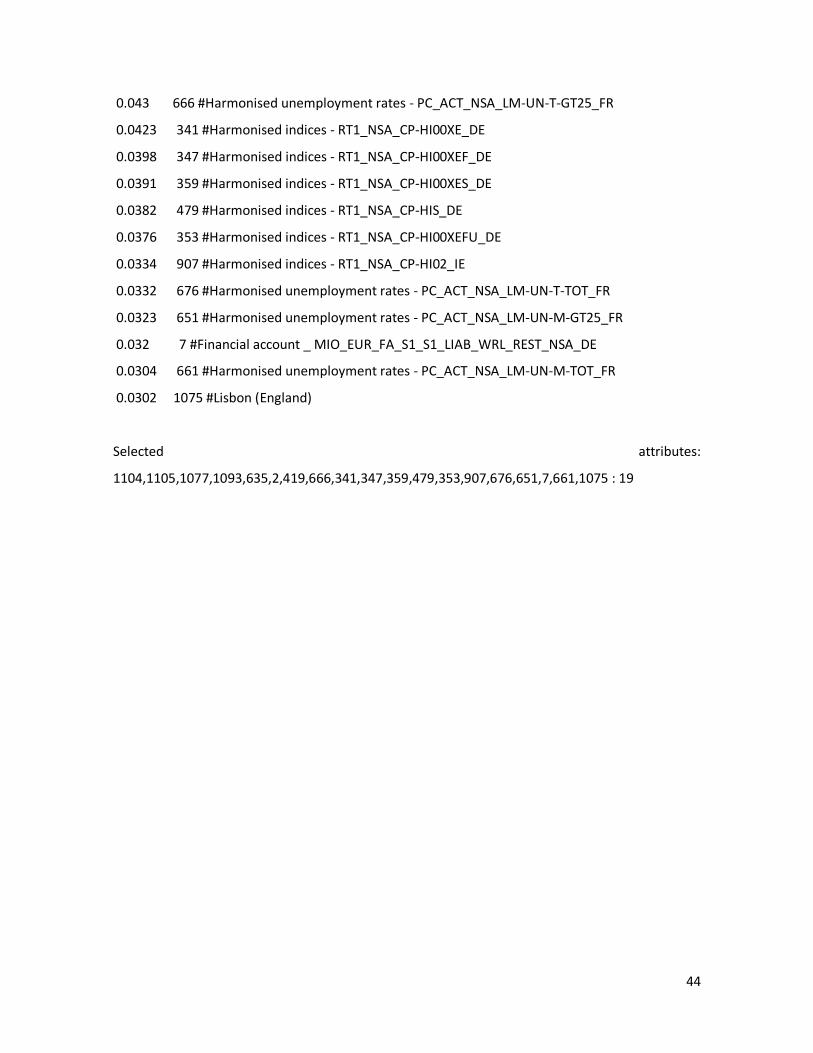
44
0.043 666 #Harmonised unemployment rates - PC_ACT_NSA_LM-UN-T-GT25_FR
0.0423 341 #Harmonised indices - RT1_NSA_CP-HI00XE_DE
0.0398 347 #Harmonised indices - RT1_NSA_CP-HI00XEF_DE
0.0391 359 #Harmonised indices - RT1_NSA_CP-HI00XES_DE
0.0382 479 #Harmonised indices - RT1_NSA_CP-HIS_DE
0.0376 353 #Harmonised indices - RT1_NSA_CP-HI00XEFU_DE
0.0334 907 #Harmonised indices - RT1_NSA_CP-HI02_IE
0.0332 676 #Harmonised unemployment rates - PC_ACT_NSA_LM-UN-T-TOT_FR
0.0323 651 #Harmonised unemployment rates - PC_ACT_NSA_LM-UN-M-GT25_FR
0.032 7 #Financial account _ MIO_EUR_FA_S1_S1_LIAB_WRL_REST_NSA_DE
0.0304 661 #Harmonised unemployment rates - PC_ACT_NSA_LM-UN-M-TOT_FR
0.0302 1075 #Lisbon (England)
Selected attributes:
1104,1105,1077,1093,635,2,419,666,341,347,359,479,353,907,676,651,7,661,1075 : 19
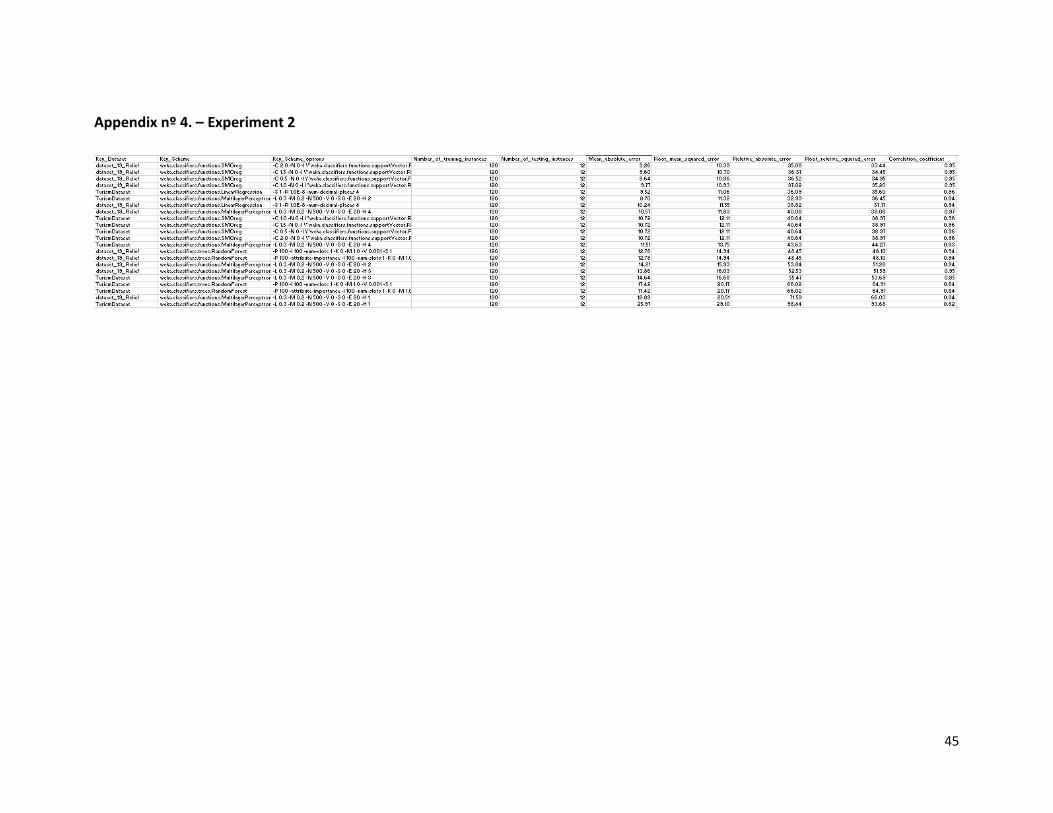
45
Appendix nº 4. – Experiment 2

46
Appendix nº 6.
=== Run information ===
Scheme: weka.classifiers.functions.SMOreg -C 2.0 -N 0 -I
"weka.classifiers.functions.supportVector.RegSMOImproved -T 0.001 -V -P 1.0E-12 -L
0.001 -W 1" -K "weka.classifiers.functions.supportVector.PolyKernel -E 1.0 -C 250007"
Relation: dataset_19_Relief
Instances: 132
Attributes: 22
#Nr_Mes
#Mes
#lagged_12m_ine_dormidas_Lisboa_Reino Unido
#lagged_1m_ine_dormidas_Lisboa_Reino Unido
#cascais (England)
#ine_hospedes_Lisboa_Reino Unido
#Harmonised unemployment rates - PC_ACT_NSA_LM-UN-F-GT25_FR
#Harmonised indices - RT1_NSA_CP-HI09_DE
#Harmonised unemployment rates - PC_ACT_NSA_LM-UN-T-GT25_FR
#Harmonised indices - RT1_NSA_CP-HI00XE_DE
#Harmonised indices - RT1_NSA_CP-HI00XEF_DE
#Harmonised indices - RT1_NSA_CP-HI00XES_DE
#Harmonised indices - RT1_NSA_CP-HIS_DE
#Harmonised indices - RT1_NSA_CP-HI00XEFU_DE
#Harmonised unemployment rates - PC_ACT_NSA_LM-UN-T-TOT_FR
#Harmonised indices - RT1_NSA_CP-HI02_IE
#Harmonised unemployment rates - PC_ACT_NSA_LM-UN-M-GT25_FR
#Financial account _ MIO_EUR_FA_S1_S1_LIAB_WRL_REST_NSA_DE
#Harmonised unemployment rates - PC_ACT_NSA_LM-UN-M-TOT_FR
#Harmonised indices - RT12_NSA_CP-HI04_EL

47
#Harmonised unemployment rates - PC_ACT_NSA_LM-UN-F-TOT_FR
#ine_dormidas_Lisboa_Reino Unido
Test mode: split 91.0% train, remainder test
=== Classifier model (full training set) ===
SMOreg
weights (not support vectors):
+ 0.0107 * (normalized) #Nr_Mes
- 0.0513 * (normalized) #Mes
+ 0.6569 * (normalized) #lagged_12m_ine_dormidas_Lisboa_Reino Unido
+ 0.4102 * (normalized) #lagged_1m_ine_dormidas_Lisboa_Reino Unido
+ 0.1242 * (normalized) #cascais (England)
+ 0.1537 * (normalized) #ine_hospedes_Lisboa_Reino Unido
- 0.1802 * (normalized) #Harmonised unemployment rates - PC_ACT_NSA_LM-UN-F-
GT25_FR
- 0.0193 * (normalized) #Harmonised indices - RT1_NSA_CP-HI09_DE
+ 0.0151 * (normalized) #Harmonised unemployment rates - PC_ACT_NSA_LM-UN-T-
GT25_FR
- 0.0113 * (normalized) #Harmonised indices - RT1_NSA_CP-HI00XE_DE
+ 0.0353 * (normalized) #Harmonised indices - RT1_NSA_CP-HI00XEF_DE
+ 0.0016 * (normalized) #Harmonised indices - RT1_NSA_CP-HI00XES_DE
- 0.2559 * (normalized) #Harmonised indices - RT1_NSA_CP-HIS_DE
+ 0.2668 * (normalized) #Harmonised indices - RT1_NSA_CP-HI00XEFU_DE
- 0.2116 * (normalized) #Harmonised unemployment rates - PC_ACT_NSA_LM-UN-T-
TOT_FR
- 0.0674 * (normalized) #Harmonised indices - RT1_NSA_CP-HI02_IE
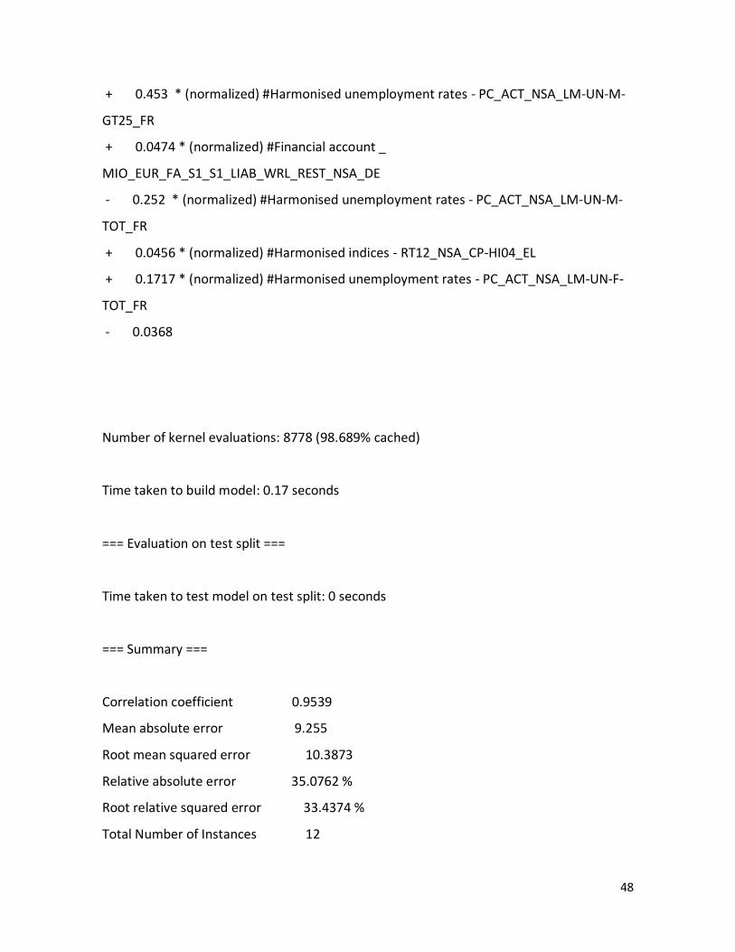
48
+ 0.453 * (normalized) #Harmonised unemployment rates - PC_ACT_NSA_LM-UN-M-
GT25_FR
+ 0.0474 * (normalized) #Financial account _
MIO_EUR_FA_S1_S1_LIAB_WRL_REST_NSA_DE
- 0.252 * (normalized) #Harmonised unemployment rates - PC_ACT_NSA_LM-UN-M-
TOT_FR
+ 0.0456 * (normalized) #Harmonised indices - RT12_NSA_CP-HI04_EL
+ 0.1717 * (normalized) #Harmonised unemployment rates - PC_ACT_NSA_LM-UN-F-
TOT_FR
- 0.0368
Number of kernel evaluations: 8778 (98.689% cached)
Time taken to build model: 0.17 seconds
=== Evaluation on test split ===
Time taken to test model on test split: 0 seconds
=== Summary ===
Correlation coefficient 0.9539
Mean absolute error 9.255
Root mean squared error 10.3873
Relative absolute error 35.0762 %
Root relative squared error 33.4374 %
Total Number of Instances 12

49
Appendix nº 7.
=== Run information ===
Scheme:weka.classifiers.functions.SMOreg -C 2.0 -N 0 -I
"weka.classifiers.functions.supportVector.RegSMOImproved -T 0.001 -V -P 1.0E-12 -L 0.001 -W 1" -
K "weka.classifiers.functions.supportVector.PolyKernel -E 1.0 -C 250007"
Relation: dataset_19_Relief-weka.filters.unsupervised.attribute.Remove-R6
Instances: 132
Attributes: 21
#Nr_Mes
#Mes
#lagged_12m_ine_dormidas_Lisboa_Reino Unido
#lagged_1m_ine_dormidas_Lisboa_Reino Unido
#cascais (England)
#Harmonised unemployment rates - PC_ACT_NSA_LM-UN-F-GT25_FR
#Harmonised indices - RT1_NSA_CP-HI09_DE
#Harmonised unemployment rates - PC_ACT_NSA_LM-UN-T-GT25_FR
#Harmonised indices - RT1_NSA_CP-HI00XE_DE
#Harmonised indices - RT1_NSA_CP-HI00XEF_DE
#Harmonised indices - RT1_NSA_CP-HI00XES_DE
#Harmonised indices - RT1_NSA_CP-HIS_DE
#Harmonised indices - RT1_NSA_CP-HI00XEFU_DE
#Harmonised unemployment rates - PC_ACT_NSA_LM-UN-T-TOT_FR
#Harmonised indices - RT1_NSA_CP-HI02_IE
#Harmonised unemployment rates - PC_ACT_NSA_LM-UN-M-GT25_FR
#Financial account _ MIO_EUR_FA_S1_S1_LIAB_WRL_REST_NSA_DE
#Harmonised unemployment rates - PC_ACT_NSA_LM-UN-M-TOT_FR
#Harmonised indices - RT12_NSA_CP-HI04_EL
#Harmonised unemployment rates - PC_ACT_NSA_LM-UN-F-TOT_FR
#ine_dormidas_Lisboa_Reino Unido
Test mode: split 91.0% train, remainder test
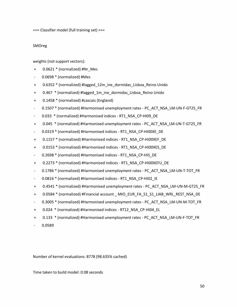
50
=== Classifier model (full training set) ===
SMOreg
weights (not support vectors):
+ 0.0621 * (normalized) #Nr_Mes
- 0.0698 * (normalized) #Mes
+ 0.6352 * (normalized) #lagged_12m_ine_dormidas_Lisboa_Reino Unido
+ 0.467 * (normalized) #lagged_1m_ine_dormidas_Lisboa_Reino Unido
+ 0.1458 * (normalized) #cascais (England)
- 0.1507 * (normalized) #Harmonised unemployment rates - PC_ACT_NSA_LM-UN-F-GT25_FR
- 0.033 * (normalized) #Harmonised indices - RT1_NSA_CP-HI09_DE
+ 0.045 * (normalized) #Harmonised unemployment rates - PC_ACT_NSA_LM-UN-T-GT25_FR
- 0.0319 * (normalized) #Harmonised indices - RT1_NSA_CP-HI00XE_DE
+ 0.1157 * (normalized) #Harmonised indices - RT1_NSA_CP-HI00XEF_DE
+ 0.0153 * (normalized) #Harmonised indices - RT1_NSA_CP-HI00XES_DE
- 0.2698 * (normalized) #Harmonised indices - RT1_NSA_CP-HIS_DE
+ 0.2273 * (normalized) #Harmonised indices - RT1_NSA_CP-HI00XEFU_DE
- 0.1786 * (normalized) #Harmonised unemployment rates - PC_ACT_NSA_LM-UN-T-TOT_FR
- 0.0816 * (normalized) #Harmonised indices - RT1_NSA_CP-HI02_IE
+ 0.4541 * (normalized) #Harmonised unemployment rates - PC_ACT_NSA_LM-UN-M-GT25_FR
+ 0.0584 * (normalized) #Financial account _ MIO_EUR_FA_S1_S1_LIAB_WRL_REST_NSA_DE
- 0.3005 * (normalized) #Harmonised unemployment rates - PC_ACT_NSA_LM-UN-M-TOT_FR
+ 0.024 * (normalized) #Harmonised indices - RT12_NSA_CP-HI04_EL
+ 0.133 * (normalized) #Harmonised unemployment rates - PC_ACT_NSA_LM-UN-F-TOT_FR
- 0.0589
Number of kernel evaluations: 8778 (98.635% cached)
Time taken to build model: 0.08 seconds

51
=== Evaluation on test split ===
Time taken to test model on test split: 0 seconds
=== Summary ===
Correlation coefficient 0.9422
Mean absolute error 6.0861
Root mean squared error 7.2737
Relative absolute error 23.0661 %
Root relative squared error 23.4146 %
Total Number of Instances 12
Final input variables:
#Mes (month) #lagged_12m_ine_dormidas_Lisboa_Reino Unido (-12 lagged target variable) #lagged_1m_ine_dormidas_Lisboa_Reino Unido (-1 lagged target variable) #cascais (England) (searched word on google) #Harmonised unemployment rates - PC_ACT_NSA_LM-UN-F-GT25_FR #Harmonised indices - RT1_NSA_CP-HI09_DE #Harmonised unemployment rates - PC_ACT_NSA_LM-UN-T-GT25_FR #Harmonised indices - RT1_NSA_CP-HI00XE_DE #Harmonised indices - RT1_NSA_CP-HI00XEF_DE #Harmonised indices - RT1_NSA_CP-HI00XES_DE #Harmonised indices - RT1_NSA_CP-HIS_DE #Harmonised indices - RT1_NSA_CP-HI00XEFU_DE #Harmonised unemployment rates - PC_ACT_NSA_LM-UN-T-TOT_FR #Harmonised indices - RT1_NSA_CP-HI02_IE #Harmonised unemployment rates - PC_ACT_NSA_LM-UN-M-GT25_FR #Financial account _ MIO_EUR_FA_S1_S1_LIAB_WRL_REST_NSA_DE #Harmonised unemployment rates - PC_ACT_NSA_LM-UN-M-TOT_FR #Harmonised indices - RT12_NSA_CP-HI04_EL #Harmonised unemployment rates - PC_ACT_NSA_LM-UN-F-TOT_FR #ine_dormidas_Lisboa_Reino Unido (target variable)

52
Appendix nº 8. – Correlations test (Spearman)

53
Appendix nº 9. – Experiment 3

54
Appendix nº 10
=== Run information ===
Scheme: weka.classifiers.functions.SMOreg -C 1.0 -N 0 -I
"weka.classifiers.functions.supportVector.RegSMOImproved -T 0.001 -V -P 1.0E-12 -L 0.001 -W 1" -K
"weka.classifiers.functions.supportVector.PolyKernel -E 1.0 -C 250007"
Relation: dataset_19_Relief-weka.filters.unsupervised.attribute.Remove-R6
Instances: 132
Attributes: 21
#Nr_Mes
#Mes
#lagged_12m_ine_dormidas_Lisboa_Reino Unido
#lagged_1m_ine_dormidas_Lisboa_Reino Unido
#cascais (England)
#Harmonised unemployment rates - PC_ACT_NSA_LM-UN-F-GT25_FR
#Harmonised indices - RT1_NSA_CP-HI09_DE
#Harmonised unemployment rates - PC_ACT_NSA_LM-UN-T-GT25_FR
#Harmonised indices - RT1_NSA_CP-HI00XE_DE
#Harmonised indices - RT1_NSA_CP-HI00XEF_DE
#Harmonised indices - RT1_NSA_CP-HI00XES_DE
#Harmonised indices - RT1_NSA_CP-HIS_DE
#Harmonised indices - RT1_NSA_CP-HI00XEFU_DE
#Harmonised unemployment rates - PC_ACT_NSA_LM-UN-T-TOT_FR
#Harmonised indices - RT1_NSA_CP-HI02_IE
#Harmonised unemployment rates - PC_ACT_NSA_LM-UN-M-GT25_FR
#Financial account _ MIO_EUR_FA_S1_S1_LIAB_WRL_REST_NSA_DE
#Harmonised unemployment rates - PC_ACT_NSA_LM-UN-M-TOT_FR
#Harmonised indices - RT12_NSA_CP-HI04_EL
#Harmonised unemployment rates - PC_ACT_NSA_LM-UN-F-TOT_FR
#ine_dormidas_Lisboa_Reino Unido
Test mode: split 91.0% train, remainder test
=== Classifier model (full training set) ===
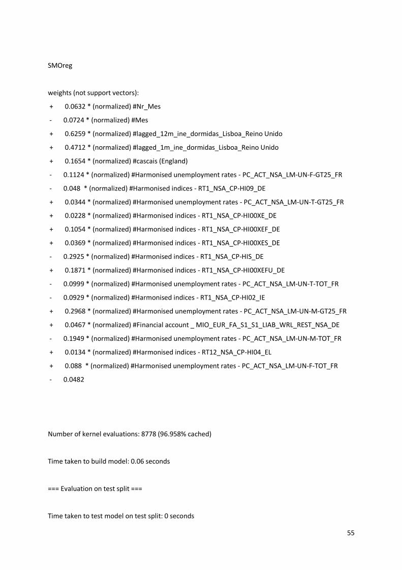
55
SMOreg
weights (not support vectors):
+ 0.0632 * (normalized) #Nr_Mes
- 0.0724 * (normalized) #Mes
+ 0.6259 * (normalized) #lagged_12m_ine_dormidas_Lisboa_Reino Unido
+ 0.4712 * (normalized) #lagged_1m_ine_dormidas_Lisboa_Reino Unido
+ 0.1654 * (normalized) #cascais (England)
- 0.1124 * (normalized) #Harmonised unemployment rates - PC_ACT_NSA_LM-UN-F-GT25_FR
- 0.048 * (normalized) #Harmonised indices - RT1_NSA_CP-HI09_DE
+ 0.0344 * (normalized) #Harmonised unemployment rates - PC_ACT_NSA_LM-UN-T-GT25_FR
+ 0.0228 * (normalized) #Harmonised indices - RT1_NSA_CP-HI00XE_DE
+ 0.1054 * (normalized) #Harmonised indices - RT1_NSA_CP-HI00XEF_DE
+ 0.0369 * (normalized) #Harmonised indices - RT1_NSA_CP-HI00XES_DE
- 0.2925 * (normalized) #Harmonised indices - RT1_NSA_CP-HIS_DE
+ 0.1871 * (normalized) #Harmonised indices - RT1_NSA_CP-HI00XEFU_DE
- 0.0999 * (normalized) #Harmonised unemployment rates - PC_ACT_NSA_LM-UN-T-TOT_FR
- 0.0929 * (normalized) #Harmonised indices - RT1_NSA_CP-HI02_IE
+ 0.2968 * (normalized) #Harmonised unemployment rates - PC_ACT_NSA_LM-UN-M-GT25_FR
+ 0.0467 * (normalized) #Financial account _ MIO_EUR_FA_S1_S1_LIAB_WRL_REST_NSA_DE
- 0.1949 * (normalized) #Harmonised unemployment rates - PC_ACT_NSA_LM-UN-M-TOT_FR
+ 0.0134 * (normalized) #Harmonised indices - RT12_NSA_CP-HI04_EL
+ 0.088 * (normalized) #Harmonised unemployment rates - PC_ACT_NSA_LM-UN-F-TOT_FR
- 0.0482
Number of kernel evaluations: 8778 (96.958% cached)
Time taken to build model: 0.06 seconds
=== Evaluation on test split ===
Time taken to test model on test split: 0 seconds

56
=== Summary ===
Correlation coefficient 0.9425
Mean absolute error 6.0237
Root mean squared error 7.2338
Relative absolute error 22.8298 %
Root relative squared error 23.2862 %
Total Number of Instances 12

57
Appendix nº 11 – Scenario 1

58
Appendix nº 12 – Scenario 2

59
Appendix nº 13 – Scenario 3