forecasting the winner of a tennis match

Forecasting the winner of a tennis match

Franc J.G.M. Klaassen a, Jan R. Magnus b,*

a Faculty of Economics and Econometrics, University of Amsterdam, Roetersstraat 11, 1018 WB Amsterdam,

The Netherlandsb Center for Economic Research (CentER), Tilburg University, P.O. Box 90153, 5000 LE Tilburg, The Netherlands

Abstract

We propose a method to forecast the winner of a tennis match, not only at the beginning of the match, but also (and

in particular) during the match. The method is based on a fast and flexible computer program, and on a statistical

analysis of a large data set from Wimbledon, both at match and at point level.

� 2002 Elsevier Science B.V. All rights reserved.

Keywords: Forecasting; Tennis; Logit; Panel data

1. Introduction

The use of statistics has become increasingly

popular in sports. TV broadcasts inform us about

the percentage of ball possession in football, the

number of home runs in baseball, the percentage

of aces and double faults in tennis, to mention justa few. All these statistics provide some insight in

the question which player or team performs par-

ticularly well in a match, and is therefore more

likely to win. However, a direct estimate of the

probability that a player (team) wins the match is

seldom shown. This is remarkable, because this

statistic is the one that viewers want to know

above all.In this paper we discuss how to estimate the

probability of winning a tennis match, not only at

the beginning of a match, but in particular while

the match is in progress. This leads to a profile of

probabilities, which unfolds during the match and

can be plotted in a graph while the match is in

progress.

The basis of the approach is our computer pro-

gram TENNISPROB, to be discussed in Section 2.

For a match between two players A and B, theprogram calculates the probability pa that A wins

the match. Let pa denote the probability that Awins a point on service, and pb the probability that

B wins a point on service. Then, under the assump-

tion that points are independent and identically

distributed (i.i.d.), the match probability pa de-

pends on the point probabilities pa and pb, the type

of tournament (best-of-3-sets or best-of-5-sets,tiebreak in final set or not), the current score, and

the current server. Our program calculates the

probabilities exactly (not by simulation) and very

fast.

The i.i.d. assumption needs some justification,

because a priori there is no reason why this as-

sumption should hold. If true, it would imply for

* Corresponding author. Tel.: +31-13-466-3092.

E-mail address: [email protected] (J.R. Magnus).

0377-2217/03/$ - see front matter � 2002 Elsevier Science B.V. All rights reserved.

doi:10.1016/S0377-2217(02)00682-3

European Journal of Operational Research 148 (2003) 257–267

www.elsevier.com/locate/dsw

mail to: [email protected]

example that a player is not influenced by the fact

whether the previous point was won or lost (in-

dependence), and also that a player is not influ-

enced by whether the current point is of particular

importance, such as a breakpoint (identical dis-

tribution). The question whether points in tennisare i.i.d. was investigated in Klaassen and Magnus

(2001). They concluded that––although points are

not i.i.d.––the deviations from i.i.d. are small and

hence the i.i.d. assumption is justified in many

applications, such as forecasting.

The computation of the match profiles has two

aspects, both of which will be addressed. First, we

need the starting point of the profile, that is pa atthe beginning of the match. Secondly, we need the

development of pa while the match is in progress.

In Section 3 we estimate pa at the start of a

match, using Wimbledon singles match data,

1992–1995. Estimation is based on a simple logit

model, where pa is determined by the difference

between the world rankings of the two players. 1

The user of the program (say, the commentator)very likely has his/her own view on pa (or, equiv-

alently, on pb ¼ 1 � pa), based on information

which is not available to us, such as an injury

problem or fear against this specific opponent. The

commentator will be able to adjust our estimate of

pa to suit his/her own views. In the end, there is

one starting point p̂pa for the profile.

To estimate pa during the match, TENNIS-PROB requires estimates of the two unknown

probabilities pa and pb. These estimates cannot be

obtained from match data. Thus, in Section 4, we

use point-to-point data of a subset of the 1992–

1995 singles matches to estimate pa þ pb. Noting

that pa at the start of the match is a function of paand pb and hence of pa � pb and pa þ pb, and that

we now have estimates of pa (from match data)and of pa þ pb, we obtain an estimate of pa � pb by

inverting the program. This gives us both p̂pa and

p̂pb.In Section 5 we demonstrate the use of the

theory and the program by drawing profiles of two

famous Wimbledon finals, Sampras–Becker (1995)

and Graf–Novotna (1993). Such profiles can be

drawn for any match, not only when the match is

completed, but also while the match is in progress.

Some conclusions are provided in Section 6,

where we also point out a few issues for furtherinvestigation.

2. The program TENNISPROB and some applica-

tions

Consider one match between two players Aand B. As motivated in the Introduction, we as-sume that points are i.i.d. (depending only on who

serves). Then, modelling a tennis match between

A and B depends on only two parameters: the

probability pa that A wins a point on service, and

the probability pb that B wins a point on service.

Given these two (fixed) probabilities, given the

rules of the tournament, given the score and who

serves the current point, one can calculate exactlythe probability of winning the current game (or

tiebreak), the current set, and the match. For ex-

ample, at the beginning of a game, the probability

that A wins a game on service is

ga ¼p4að�8p3

a þ 28p2a � 34pa þ 15Þ

p2a þ ð1 � paÞ2

: ð1Þ

The program TENNISPROB is an efficient

(and very fast) computer program which calculates

these probabilities. The probabilities are calculatedexactly; they are not simulated. The program is

flexible, because it allows the user to specify the

score and to adjust to the particularities of the

tournament, but also because it allows for rule

changes. For example, if the traditional scoring

rule at deuce is replaced by the alternative of

playing one deciding point at deuce (�sudden

death�), 2 then the probability that server A winsthe game changes from (1) to

1 See Boulier and Stekler (1999), Clarke and Dyte (2000),

and Lebovic and Sigelman (2001) on the forecasting accuracy of

rankings and related issues.

2 Rule 26b of the ‘‘Rules of Tennis 2000’’, approved by the

International Tennis Federation, allows for this optional

scoring system. At deuce, one deciding point is played, whereby

the receiver may choose whether to receive the service from the

right-half or the left-half of the court.

258 F.J.G.M. Klaassen, J.R. Magnus / European Journal of Operational Research 148 (2003) 257–267

g�a ¼ p4a

�� 20p3

a þ 70p2a � 84pa þ 35

�: ð2Þ

A simple calculation shows that for every pa > 0:5(the most common case), we have g�a < ga, so that

more service breaks will occur. The largest dis-

crepancy occurs at pa ¼ 0:65, where ga ¼ 0:830

and g�a ¼ 0:800, and the probability of a break thusincreases from 17% to 20%.

As another example of the flexibility of the

program, we can analyze what would happen if the

tournament requires 4 games rather than 6 to be

won in order to win a set (not currently allowed by

the official rules). As expected, we find that the

advantage for the �better� player is somewhat re-

duced under this rule change.The program can also be used to calculate the

importance of a point, defined by Morris (1977) as

the probability that A wins the match if he/she

wins the current point minus the probability that

A wins the match if he/she loses the current point.

The definition implies that the importance of a

point is the same for A and B. TENNISPROB

can tell us what the important points of a matchare, and we will plot these in the profiles of Figs. 5

and 6.

In order to compute the probability pa that

player A wins the match, the program needs both

pa and pb, or, equivalently, pa � pb (the difference

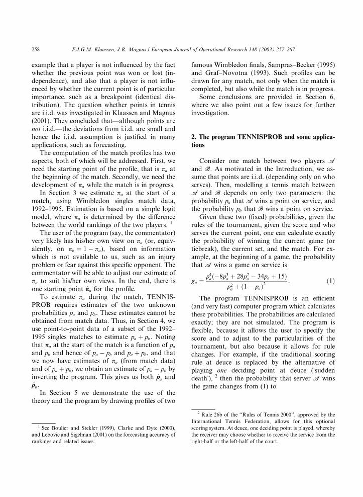
in strength between the two players) and pa þ pb(the overall quality of a match). One would expect

that pa � pb is much more important than pa þ pb.This is indeed the case, as we now demonstrate.

Given the type of tournament and an equal score,

pa is a function of pa � pb, pa þ pb and the score,but does not depend on who serves at this point. In

Fig. 1 we analyze the dependence of pa on pa � pbfor different values of pa þ pb. Fig. 1 (Panel A)

gives the probability pa at the start of a best-of-5-

sets match, as played by the men in grand slam

tournaments such as Wimbledon. For given pa þpb, pa is a monotonically increasing function of

pa � pb, and this functional dependence is given byan S-shaped curve. The collection of all curves for

0:8 < pa þ pb < 1:6 (the empirically relevant inter-

val at Wimbledon), gives the fuzzy S-shaped curve

of Fig. 1A. The message from Fig. 1A is that pa

depends almost entirely on pa � pb and only very

slightly on pa þ pb, a fact also reported in Alefeld

(1984). The same is true at the beginning of the

third set (at 1-1 in sets) and even (remarkably) atthe beginning of the final set.

In Fig. 1 (Panel B) we present pa at 5-5 in the

final set. We conclude that at the beginning of a

match the probability pa is explained almost ex-

clusively by pa � pb, but that the dependence on

pa þ pb increases towards the end of a match.

Fig. 1. Probability pa that A wins match as a function of quality difference, two equal scores, best-of-5-sets match.

F.J.G.M. Klaassen, J.R. Magnus / European Journal of Operational Research 148 (2003) 257–267 259

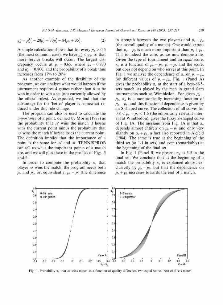
The situation is different when the score is not

equal. Fig. 2 gives the probabilities when A is

serving in the final set at 5-4 (Fig. 2, Panel A) and

4-5 (Fig. 2, Panel B), respectively. The dependence

on pa þ pb is much larger now, emphasizing that atunequal scores a good estimate of pa þ pb is re-

quired to forecast the winner, especially at the later

stages of a match.

3. Estimation of pa at the start of a match, based on

match data

In this section we estimate the probability pa

that A wins the match, at the start of the match.

This will be the first point of the match profile.

We have data on all singles matches played at

Wimbledon 1992–1995. In each year 128 men and

128 women compete for the singles titles. Thus, for

both men and women, 127 matches are played

annually, leading to 508 matches over four years.Some matches are broken off due to injury or de-

fault, and these matches have been removed from

our sample. This leaves 495 matches in the men�ssingles and 504 matches in the women�s singles.

For each match we know the two players, their

rankings, and the winner.

The rankings of the players are determined by

the lists published just before Wimbledon by the

Association of Tennis Professionals (ATP) for the

men, and the Women�s Tennis Association (WTA)

for the women. These two lists contain the officialrankings based on performances over the last 52

weeks, including last year�s Wimbledon. The

ranking of player A is denoted RANKa.

Direct use of the rankings is not satisfactory,

because quality in tennis is a pyramid: the differ-

ence between the top two players (ranked 1 and 2)

is generally larger than between two players ranked

101 and 102 (see also Lebovic and Sigelman, 2001).The pyramid is based on �round in which we expect

the player to lose�. For example, 3 for a player

who is expected to lose in round 3, 7 for a player

who is expected to reach the final (round 7) and

lose, and 8 for the player who is expected to win the

final.

A problem with �expected round� is that it

does not distinguish, for example, between play-ers ranked 9–16 since all of them are expected to

lose in round 4. Thus we propose a smoother

measure of �expected round� by transforming the

ranking of each player into a variable R as fol-

lows:

Ra ¼ 8 � log2 ðRANKaÞ: ð3Þ

Fig. 2. Probability pa that A wins match as a function of quality difference, two unequal scores, final set.


For example, if RANK ¼ 3 then R ¼ 6:42, while if

RANK ¼ 4 then R ¼ 6:00. 3

We shall always assume, obviously without loss

of generality, that A is the �better� player in the

sense that Ra > Rb. The better player does not al-ways win. At Wimbledon 1992–1995 the better

player won 68% of the matches in the men�s singles

and 75% of the matches in the women�s singles. So,

upsets occur regularly, especially in the men�ssingles.

Now, let pj be the probability that the �better�player (that is, player A) wins the jth match

(j ¼ 1; . . . ;N ), where N ¼ 495 in the men�s singlesand N ¼ 504 in the women�s singles. We assume a

simple logit model,

pj ¼expðFjÞ

1 þ expðFjÞ;

where Fj is a function of the (transformed) rank-

ings Ra and Rb.4 Let Dj � Ra � Rb. If Dj ¼ 0, then

Ra ¼ Rb and both players are equally strong. We

would expect in that case that pj ¼ 0:5 and hence

that Fj ¼ 0. This implies that Fj ¼ kDj, where k can

be a constant or a function of other variables.

After testing various specifications for k ¼kðRa;RbÞ, we conclude that the simplest specifica-

tion is the best. 5 Thus we take k to be a constant,

so that

pj ¼expðkDjÞ

1 þ expðkDjÞ: ð4Þ

Let zj ¼ 1 if player A wins the jth match, and 0

otherwise. Then the likelihood of the sample is

given by L ¼QN

j¼1 pzjj ð1 � pjÞ1�zj . Estimating k by

maximum likelihood gives k̂k ¼ 0:3986 (0.0461) in

the men�s singles, and k̂k ¼ 0:7150 (0.0683) in the

women�s singles, with the standard errors given inparentheses. For example, for Ra ¼ 8 and Rb ¼ 4

(that is, number 1 against number 16 in the official

rankings), we find p̂pa ¼ 0:8312 in the men�s singles

and p̂pa ¼ 0:9458 in the women�s singles.

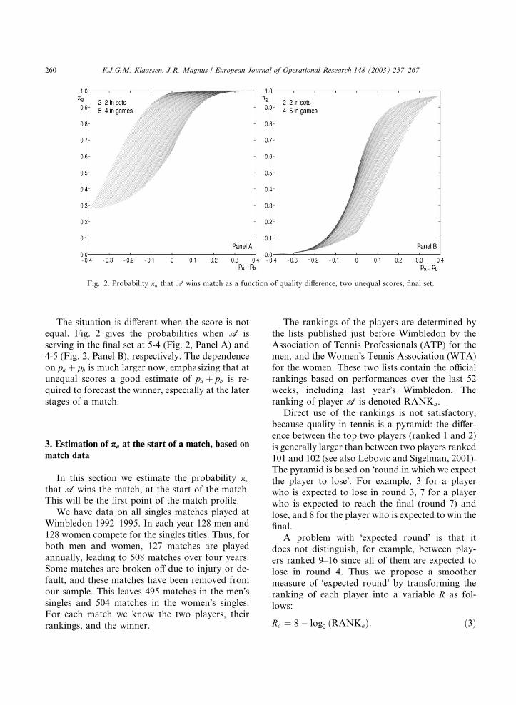
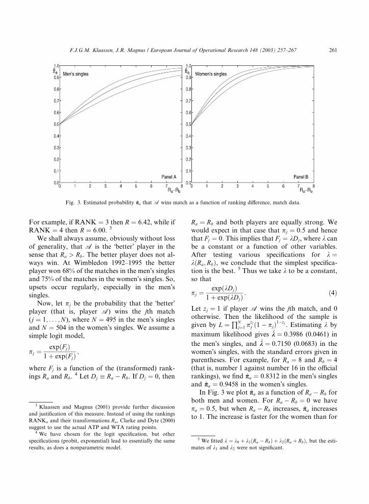
In Fig. 3 we plot p̂pa as a function of Ra � Rb for

both men and women. For Ra � Rb ¼ 0 we have

pa ¼ 0:5, but when Ra � Rb increases, p̂pa increases

to 1. The increase is faster for the women than for

Fig. 3. Estimated probability p̂pa that A wins match as a function of ranking difference, match data.

3 Klaassen and Magnus (2001) provide further discussion

and justification of this measure. Instead of using the rankings

RANKa and their transformations Ra, Clarke and Dyte (2000)

suggest to use the actual ATP and WTA rating points.4 We have chosen for the logit specification, but other

specifications (probit, exponential) lead to essentially the same

results, as does a nonparametric model.

5 We fitted k ¼ k0 þ k1ðRa � RbÞ þ k2ðRa þ RbÞ, but the esti-

mates of k1 and k2 were not significant.


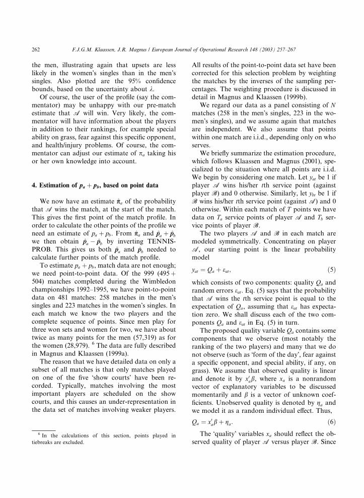
the men, illustrating again that upsets are less

likely in the women�s singles than in the men�ssingles. Also plotted are the 95% confidence

bounds, based on the uncertainty about k.

Of course, the user of the profile (say the com-

mentator) may be unhappy with our pre-matchestimate that A will win. Very likely, the com-

mentator will have information about the players

in addition to their rankings, for example special

ability on grass, fear against this specific opponent,

and health/injury problems. Of course, the com-

mentator can adjust our estimate of pa taking his

or her own knowledge into account.

4. Estimation of pa þ pb, based on point data

We now have an estimate p̂pa of the probability

that A wins the match, at the start of the match.

This gives the first point of the match profile. In

order to calculate the other points of the profile we

need an estimate of pa þ pb. From p̂pa and p̂pa þ p̂pbwe then obtain p̂pa � p̂pb by inverting TENNIS-

PROB. This gives us both p̂pa and p̂pb needed to

calculate further points of the match profile.

To estimate pa þ pb, match data are not enough;

we need point-to-point data. Of the 999 (495þ504) matches completed during the Wimbledon

championships 1992–1995, we have point-to-point

data on 481 matches: 258 matches in the men�ssingles and 223 matches in the women�s singles. In

each match we know the two players and the

complete sequence of points. Since men play for

three won sets and women for two, we have about

twice as many points for the men (57,319) as for

the women (28,979). 6 The data are fully described

in Magnus and Klaassen (1999a).

The reason that we have detailed data on only asubset of all matches is that only matches played

on one of the five �show courts� have been re-

corded. Typically, matches involving the most

important players are scheduled on the show

courts, and this causes an under-representation in

the data set of matches involving weaker players.

All results of the point-to-point data set have been

corrected for this selection problem by weighting

the matches by the inverses of the sampling per-

centages. The weighting procedure is discussed in

detail in Magnus and Klaassen (1999b).

We regard our data as a panel consisting of Nmatches (258 in the men�s singles, 223 in the wo-

men�s singles), and we assume again that matches

are independent. We also assume that points

within one match are i.i.d., depending only on who

serves.

We briefly summarize the estimation procedure,

which follows Klaassen and Magnus (2001), spe-

cialized to the situation where all points are i.i.d.We begin by considering one match. Let yat be 1 if

player A wins his/her tth service point (against

player B) and 0 otherwise. Similarly, let ybt be 1 if

B wins his/her tth service point (against A) and 0

otherwise. Within each match of T points we have

data on Ta service points of player A and Tb ser-

vice points of player B.

The two players A and B in each match aremodeled symmetrically. Concentrating on player

A, our starting point is the linear probability

model

yat ¼ Qa þ eat; ð5Þ

which consists of two components: quality Qa and

random errors eat. Eq. (5) says that the probability

that A wins the tth service point is equal to the

expectation of Qa, assuming that eat has expecta-

tion zero. We shall discuss each of the two com-ponents Qa and eat in Eq. (5) in turn.

The proposed quality variable Qa contains some

components that we observe (most notably the

ranking of the two players) and many that we do

not observe (such as �form of the day�, fear against

a specific opponent, and special ability, if any, on

grass). We assume that observed quality is linear

and denote it by x0ab, where xa is a nonrandomvector of explanatory variables to be discussed

momentarily and b is a vector of unknown coef-

ficients. Unobserved quality is denoted by ga and

we model it as a random individual effect. Thus,

Qa ¼ x0ab þ ga: ð6ÞThe �quality� variables xa should reflect the ob-

served quality of player A versus player B. Since

6 In the calculations of this section, points played in

tiebreaks are excluded.


Ra and Rb (discussed in Section 3) are the only

observed quality variables available, we write

x0a ¼ ð1; ðRa � RbÞ; ðRa þ RbÞÞ; ð7Þ

since both Ra � Rb (relative quality, gap between

the two players) and Ra þ Rb (absolute quality,

overall quality of the match) are potentially im-

portant, and we let b ¼ ðb0;b1; b2Þ0

denote the

corresponding vector of three unknown parame-

ters.

Because the observed part contains a constant

term, there is no loss in generality in assumingEðgaÞ ¼ EðgbÞ ¼ 0. In addition, we impose

varðgaÞ ¼ varðgbÞ ¼ s2; covðga; gbÞ ¼ c; ð8Þ

where jcj < s2. The covariance c captures the idea

that if A performs better on service than the

rankings suggest, then one would expect that the

probability that B will win a point on service is

lower.

The second component in (5) is the error term

eat. The error is affected by the binary structure ofyat, because it can only take the values 0 � Qa and

1 � Qa. We assume that EðeatÞ ¼ 0. Regarding the

second moments we make the standard assump-

tions

covðeat; gaÞ ¼ covðeat; gbÞ ¼ 0;

covðeat; easÞ ¼ 0 ðs 6¼ tÞ; covðeat; ebsÞ ¼ 0: ð9Þ

However, the usual assumption that the variance

of eat is homoskedastic is not reasonable in our

case, because of the binary character of the ob-

servations. Since EðyatÞ ¼ Eðy2atÞ, we obtain

varðeatÞ ¼ ðx0abÞð1 � x0abÞ � s2; ð10Þ

so that varðeatÞ depends on a. Hence we must take

proper account of heteroskedasticity.

Assumptions (5)–(10) imply the following bi-

nary panel model with random effects:

yat ¼ x0ab þ uat; uat ¼ ga þ eat; ð11Þ

and similarly for player B. Stacking the fuatg into

Ta 1 vectors ua, and defining ia as the Ta 1

vector of ones and ITa as the Ta Ta identity ma-

trix, the T T variance matrix of the error vector

ðu0a; u0bÞ0of the whole match is given by

X ¼ varuaub

� �

¼ r2aITa þ s2iai0a ciai0b

cibi0a r2bITb þ s2ibi0b

� �: ð12Þ

In order to estimate the five unknown parameters

(three b�s, s2 and c), we take averages and obtain

�yya�yyb

� ��

x0abx0bb

� �;

x2a c

c x2b

� �!; ð13Þ

where

x2a ¼

Ta � 1

Tas2 þ ðx0abÞð1 � x0abÞ

Ta;

x2b ¼

Tb � 1

Tbs2 þ ðx0bbÞð1 � x0bbÞ

Tb:

Assuming normality for the averages and taking

full account of the variance restrictions, we esti-

mate the parameters by maximum likelihood. The

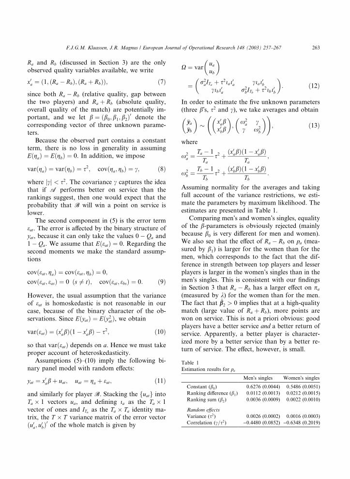
estimates are presented in Table 1.Comparing men�s and women�s singles, equality

of the b-parameters is obviously rejected (mainly

because b0 is very different for men and women).

We also see that the effect of Ra � Rb on pa (mea-

sured by b1) is larger for the women than for the

men, which corresponds to the fact that the dif-

ference in strength between top players and lesser

players is larger in the women�s singles than in themen�s singles. This is consistent with our findings

in Section 3 that Ra � Rb has a larger effect on pa

(measured by k) for the women than for the men.

The fact that b̂b2 > 0 implies that at a high-quality

match (large value of Ra þ Rb), more points are

won on service. This is not a priori obvious: good

players have a better service and a better return of

service. Apparently, a better player is character-ized more by a better service than by a better re-

turn of service. The effect, however, is small.

Table 1

Estimation results for pa

Men�s singles Women�s singles

Constant (b0) 0.6276 (0.0044) 0.5486 (0.0051)

Ranking difference (b1) 0.0112 (0.0013) 0.0212 (0.0015)

Ranking sum (b2) 0.0036 (0.0009) 0.0022 (0.0010)

Random effects

Variance (s2) 0.0026 (0.0002) 0.0016 (0.0003)

Correlation (c=s2) )0.4480 (0.0852) )0.6348 (0.2019)


We estimate the probabilities pa and pb by x0ab̂band x0bb̂b, respectively. This gives

p̂pa þ p̂pb ¼ 2ðb̂b0 þ ðRa þ RbÞb̂b2Þ:It is clear that p̂pa þ p̂pb increases with Ra þ Rb, since

b̂b2 > 0, and also that the increase is very slight,

since b̂b2 is small.

We now have an estimate of pa from Section 3

and an estimate of pa þ pb from the current sec-

tion. By inverting TENNISPROB we then obtainan estimate of pa � pb, and hence of pa and pb.These are the estimates used in computing the

profiles.

Of course, we could have estimated pa � pb di-

rectly from the point data, because the analysis in

the current section yields estimates of both pa þ pband pa � pb. In fact,

p̂pa � p̂pb ¼ 2ðRa � RbÞb̂b1:

Given the estimates p̂pa and p̂pb obtained from point

data, we obtain an alternative estimator of pa at

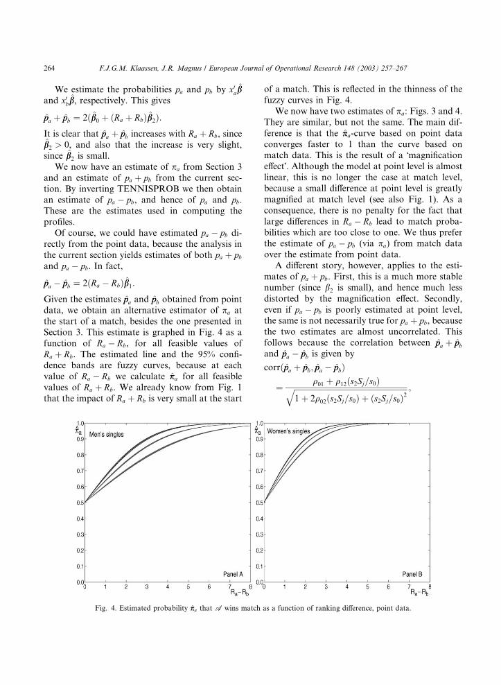
the start of a match, besides the one presented inSection 3. This estimate is graphed in Fig. 4 as a

function of Ra � Rb, for all feasible values of

Ra þ Rb. The estimated line and the 95% confi-

dence bands are fuzzy curves, because at each

value of Ra � Rb we calculate p̂pa for all feasible

values of Ra þ Rb. We already know from Fig. 1

that the impact of Ra þ Rb is very small at the start

of a match. This is reflected in the thinness of the

fuzzy curves in Fig. 4.

We now have two estimates of pa: Figs. 3 and 4.

They are similar, but not the same. The main dif-

ference is that the p̂pa-curve based on point dataconverges faster to 1 than the curve based on

match data. This is the result of a �magnification

effect�. Although the model at point level is almost

linear, this is no longer the case at match level,

because a small difference at point level is greatly

magnified at match level (see also Fig. 1). As a

consequence, there is no penalty for the fact that

large differences in Ra � Rb lead to match proba-bilities which are too close to one. We thus prefer

the estimate of pa � pb (via pa) from match data

over the estimate from point data.

A different story, however, applies to the esti-

mates of pa þ pb. First, this is a much more stable

number (since b2 is small), and hence much less

distorted by the magnification effect. Secondly,

even if pa � pb is poorly estimated at point level,the same is not necessarily true for pa þ pb, because

the two estimates are almost uncorrelated. This

follows because the correlation between p̂pa þ p̂pband p̂pa � p̂pb is given by

corrðp̂pa þ p̂pb; p̂pa � p̂pbÞ

¼ q01 þ q12ðs2Sj=s0Þffiffiffiffiffiffiffiffiffiffiffiffiffiffiffiffiffiffiffiffiffiffiffiffiffiffiffiffiffiffiffiffiffiffiffiffiffiffiffiffiffiffiffiffiffiffiffiffiffiffiffiffiffiffiffiffiffiffiffi1 þ 2q02ðs2Sj=s0Þ þ ðs2Sj=s0Þ2

q ;

Fig. 4. Estimated probability p̂pa that A wins match as a function of ranking difference, point data.


where si denotes the standard error of b̂bi, qij de-

notes the estimated correlation between b̂bi and b̂bj,

and Sj ¼ Ra þ Rb in the jth match. 7 The estimated

correlation is very small: smaller than 0.10 for the

men and smaller than 0.08 for the women (in ab-solute value). Hence, p̂pa þ p̂pb and p̂pa � p̂pb are al-

most independent.

5. Forecasts and profiles

Based on the previous discussion, our forecast

strategy is as follows. Before the start of a givenmatch, we know Ra and Rb. This gives us an esti-

mate of pa based on match data (Fig. 3), possibly

adjusted by the commentator. We also have an

estimate of pa þ pb based on point data. For given

pa þ pb, pa at the start of a match is a monotonic

function of pa � pb. Hence, by inverting TEN-

NISPROB, we obtain an estimate of pa � pb as

well. We thus find estimates of pa þ pb and pa � pband hence of pa and pb. With these estimates we

can calculate the probability that A wins the

match at each point in the match, using TEN-

NISPROB.

To illustrate the theory developed in this paper

we shall draw profiles of two important Wimble-

don finals. The first match is the 1995 men�s final

Sampras–Becker. Here Sampras (player A) wasthe favourite, having RANK ¼ 2 and hence Ra ¼7, while Becker (player B) had RANK ¼ 4 and

Rb ¼ 6. Our pre-match estimates are that Sampras

has a 59.8% chance of winning the championship

(p̂pa ¼ 0:5983), and that p̂pa þ p̂pb ¼ 1:3487. As a

consequence, we calculate that p̂pa � p̂pb ¼ 0:0161,

and hence that the estimates of pa and pb are

p̂pa ¼ 0:6824 and p̂pb ¼ 0:6663. There are many linesin Fig. 5. We first discuss the central profile which

starts at p̂pa ¼ 0:5983. The first set goes to a tie-

break. After losing the tiebreak, Sampras� proba-

bility of winning has decreased to 39.6%. In the

second set, Sampras breaks Becker�s service at 1-1

and again at 3-1, and wins the set. In the third and

fourth sets, Becker�s service is broken again three

times. The last break (at 4-2 in the fourth set) in-

creases Sampras�s chances only marginally, since

he is already almost certain to win. Eventually

Sampras wins 6-7, 6-2, 6-4, 6-2 after 246 points.

The two fuzzy curves just above and below thecentral profile both consist of two curves. Each of

these four additional curves is based on a different

combination of pa and pa þ pb. The upper two,

hardly distinguishable, curves are based on the

upper 95% confidence bound for pa (see Fig. 3) in

combination with either the upper or the lower

95% confidence bound for pa þ pb. The lower two

curves are based on the lower 95% confidencebound for pa with either the upper or the lower

95% confidence bound for pa þ pb. What we see is

that the level of the profile can shift a bit, but that

the movement of the profile is not affected when

the initial estimates of pa and pa þ pb and thus paand pb, are somewhat biased. Even when we sim-

ply take p̂pa ¼ 0:5 at the start of the match (also

plotted), the movement of the profile is the same.We conclude that the level of the profile depends

on the correct estimation of pa and pb, but that the

movement of the profile is robust.

The bottom part of Fig. 5 shows the importance

of each point, as defined in Section 2. One can

clearly see the importance of the tiebreak at the

end of the first set, and in particular the last point

of the tiebreak (Becker�s setpoint at 6-5), which isthe most important point of the whole match

(imp ¼ 0:19). Also important are the four break-

points at 1-1 in the third set.

In the second plot we only show the central

profile (and the 50% line: at points above the 50%

line we expect A to win, at points below the line

we expect B to win). This is the plot that one may

want to show to a television audience, updatedafter every few games. This profile concerns the

famous 1993 women�s singles final Graf–Novotna

(Fig. 6). Graf (player A) was the favourite, having

RANK ¼ 1 and hence Ra ¼ 8, while Novotna had

RANK ¼ 9 and hence Rb ¼ 4:83. Our pre-match

estimates are that Graf has a 90.6% chance of

winning (p̂pa ¼ 0:9060), and that p̂pa þ p̂pb ¼ 1:1538.

As a consequence, we calculate that p̂pa � p̂pb ¼0:0992, and hence that the estimates of pa and pbare p̂pa ¼ 0:6265 and p̂pb ¼ 0:5273.

7 The estimated correlations for the men (women) are

q01 ¼ 0:0052 (0.0865), q02 ¼ �0:8568 ()0.8898), and q12 ¼0:0353 ()0.0533).


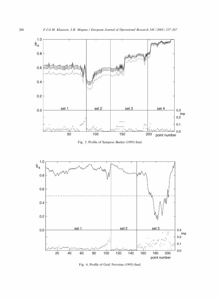
Fig. 6. Profile of Graf–Novotna (1993) final.

Fig. 5. Profile of Sampras–Becker (1995) final.


The first set goes to a tiebreak. At the beginning

of the tiebreak (point 93), Graf�s probability of

winning has decreased a little to 85.9%. After

winning the tiebreak, the probability jumps to

96.5% (point 107). Novotna wins the second set

easily. At the beginning of the third set, Graf�sprobability of winning is still 81.7% (point 149). At

1-1 in the third set Graf�s service is broken, and at

3-1 again. When Novotna serves at 4-1, 40-30

(point 183), Graf�s probability of winning has

dropped to 14.9%. Then Graf breaks back, and

holds service (after two breakpoints). When Nov-

otna serves at 4-3, 40-40, the match is in the bal-

ance. This is the most important game of thematch and the two breakpoints in this game are

the most important points of the match (imp ¼0:27). Novotna loses the second breakpoint, the

next two games, and the match. Graf wins 7-6, 1-6,

6-4 after 210 points.

6. Conclusion

In this paper we have described a method of

forecasting the outcome of a tennis match. More

precisely, we have estimated the probability that

one of the two players wins the match, not only at

the beginning of the match but also as the match

unfolds. The calculations are based on a flexible

computer program TENNISPROB and on esti-mates using Wimbledon singles data 1992–1995,

both at match level and at point level.

The methodology described in the paper rests

on two basic assumptions. First, we assume that

points are i.i.d., so that pa and pb stay fixed during

the match. As we have demonstrated in Klaassen

and Magnus (2001), points are not i.i.d., but the

deviations from i.i.d. are small, so that in parti-cular applications (such as forecasting) the i.i.d.

assumption will provide a sufficiently good ap-

proximation.

In addition, we also assume that the estimates

p̂pa and p̂pb, obtained before the match starts, are not

updated during the match. That is, we don�t use

information of the points played up to the current

point. One could think of a Bayesian updating

rule, where the prior estimates are p̂pa and p̂pb, ob-

tained before the match starts, and the likelihood

comprises the match information up to the current

point. This would lead to posterior estimates of

pa and pb. Whether the forecast error is actuallyreduced by such a refinement is still an open

question.

Acknowledgements

The authors are grateful to IBM UK and The

All England Lawn Tennis and Croquet Club atWimbledon for their kindness in providing the

data, to Ruud Koning and the referee for useful

comments, and to Dmitri Danilov for help with

the pictures.

References

Alefeld, B., 1984. Statistische Grundlagen des Tennisspiels.

Leistungssport 3, 43–46.

Boulier, B.L., Stekler, H.O., 1999. Are sports seedings good

predictors? An evaluation. International Journal of Fore-

casting 15, 83–91.

Clarke, S.R., Dyte, D., 2000. Using official ratings to simulate

major tennis tournaments. International Transactions in

Operational Research 7, 585–594.

Klaassen, F.J.G.M., Magnus, J.R., 2001. Are points in tennis

independent and identically distributed? Evidence from a

dynamic binary panel data model. Journal of the American

Statistical Association 96, 500–509.

Lebovic, J.H., Sigelman, L., 2001. The forecasting accuracy and

determinants of football rankings. International Journal of

Forecasting 17, 105–120.

Magnus, J.R., Klaassen, F.J.G.M., 1999a. On the advantage of

serving first in a tennis set: Four years at Wimbledon. The

Statistician (Journal of the Royal Statistical Society, Series

D) 48, 247–256.

Magnus, J.R., Klaassen, F.J.G.M., 1999b. The effect of new

balls in tennis: Four years at Wimbledon. The Statistician

(Journal of the Royal Statistical Society, Series D) 48, 239–

246.

Morris, C., 1977. The most important points in tennis. In:

Ladany, S.P., Machol, R.E. (Eds.), Optimal Strategies in

Sport. North-Holland Publishing Company, Amsterdam,

pp. 131–140.


forecasting the winner of a tennis match

Documents