forecasting: the first step in demand planningjrclass/sca/notes/2-forecasting.pdf · forecasting:...

Department of Industrial Engineering

Forecasting: The First Step in Demand Planning

Jayant Rajgopal, Ph.D., P.E. Department of Industrial Engineering University of Pittsburgh Pittsburgh, PA 15261


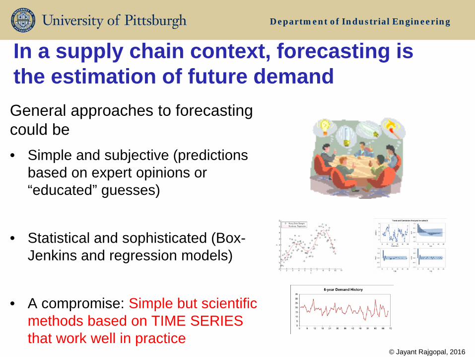
In a supply chain context, forecasting is the estimation of future demand General approaches to forecasting could be • Simple and subjective (predictions

based on expert opinions or “educated” guesses)

• Statistical and sophisticated (Box-Jenkins and regression models)

• A compromise: Simple but scientific methods based on TIME SERIES that work well in practice

© Jayant Rajgopal, 2016


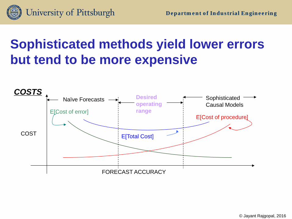
Sophisticated methods yield lower errors but tend to be more expensive


E[Cost of procedure] E[Cost of error]

E[Total Cost]

Naïve Forecasts Sophisticated Causal Models

Desired operating range

COST

FORECAST ACCURACY

COSTS


A general forecasting framework


Qualitative Analysis

Forecast

Control

Forecasting Procedure

Past data

Actual Demand

Final Forecast


A good forecasting procedure should yield ACCURATE and UNBIASED forecasts

Some things to keep in mind

• There is no single “best” forecasting model for any dataset

• Forecasts are typically wrong!

• Most planners/managers like a range of values for the forecast rather than one single number

• Aggregate forecasts are always more accurate than individual ones

• Forecast accuracy decreases as the forecast horizon increases



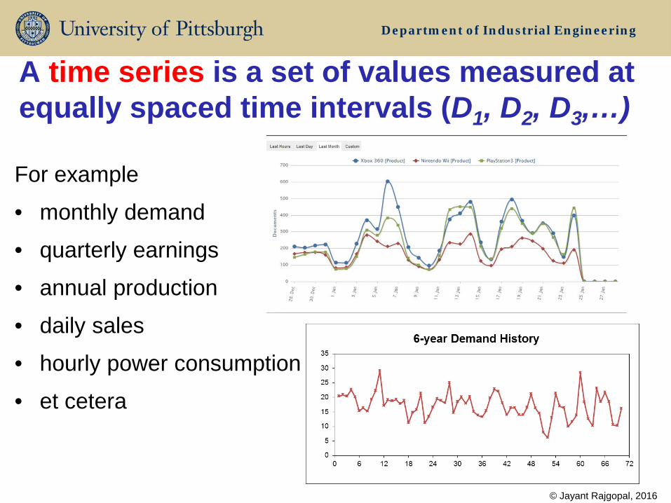
A time series is a set of values measured at equally spaced time intervals (D1, D2, D3,…)

For example

• monthly demand

• quarterly earnings

• annual production

• daily sales

• hourly power consumption

• et cetera



Possible Components of a time series


Level (L) - always Level + Trend (T)

Level + Seasonality (S) Level + Trend + Seasonality

Important: In all cases there is randomness!


Suppose we are now at the end of period t. Then the forecast for a future period j>t is:

The most common forecast is the one-step-ahead (o-s-a) forecast, i.e., E [Dt+1 | Dt, Dt-1, Dt-2,…]

However, we might also be interested in looking further into the future with a k-steps-ahead (k-s-a) forecast:

E [Dt+k | Dt, Dt-1, Dt-2,…]


E [Dj | Dt, Dt-1, Dt-2,…]; j>t


Notational conventions we will use:

Forecast origin t: when (i.e., end of which period) forecast is being made

Forecast horizon k: for how far ahead it is being made

Then Ft,t+k is the forecast made at the end of period t for period t+k: Ft,t+k = E [Dt+k | Dt, Dt-1, Dt-2,….]

E.g.

If t=10, k=4 , then F10,14 is the 4-step-ahead forecast for t=14 made at the end of t=10 (based on all data up to and including D10):

F10,14 = E [D14 | D10, D9, …] © Jayant Rajgopal, 2016

0 2 4 6 8 10 12 14 16

4


There are two broad approaches to handle time series data • Statistical Approach

– Assumes that the data can be statistically modeled, i.e., there is some underlying statistical process driving the data

– e.g., Dt = β1Dt-1 + β2Dt-2 + εt where εt ~N(0,σ2)

• Heuristic Approach – Does not worry about any statistical model – just uses “sensible” rules

to forecast



Level Time Series (no trends or seasonality)

Locally Constant Mean Model: Dt = Lt + εt

Our model will be based on estimating the level Lt at time t (let’s denote this estimate by 𝐿�𝑡). This estimate of the level becomes our forecast at time t for all points in the future:

Ft,t+1 = Ft,t+2 = …Ft,t+k = … = 𝐿�𝑡


one-step-ahead (o-s-a) forecast at time t

2-step-ahead forecast at time t

k-step-ahead forecast at time t


Since the level varies over time, our estimates of the level must be updated as we get new data

Suppose we just observed Dt+1

Then for the future we will now forecast via

Ft+1,t+2 = Ft+1,t+3 = …Ft+1,t+1+k = … = 𝐿�𝑡+1

t+1 Current estimate 𝐿�𝑡 (=Ft,t+1=Ft,t+1=Ft,t+1=…)

actual demand Dt+1

Updated estimate of level 𝐿�𝑡+1



Dt-2 Dt-1 Dt Ft,t+1 Ft,t+2 Ft,t+3 Ft,t+4

Here is a visual representation:


At the end of t Ft,t+k=

t-2 t-1 t t+1 t+2 t+3 t+4

Dt-2 Dt-1 Dt Dt+1 Ft+1,t+2 Ft+1,t+3 Ft+1,t+4

At the end of t+1 Ft+1,t+1+k=

t-2 t-1 t t+1 t+2 t+3 t+4

Dt-2 Dt-1 Dt Dt+1 Dt+2 Ft+2,t+3 Ft+2,t+4


t-2 t-1 t t+1 t+2 t+3 t+4

Dt-2 Dt-1 Dt Dt+1 Dt+2 Dt+3 Ft+3,t+4


t-2 t-1 t t+1 t+2 t+3 t+4

𝐿�𝑡

𝐿�𝑡+1

𝐿�𝑡+2

𝐿�𝑡+3


METHOD 1: Updating via Moving Averages


• Use the average of the N most recent observations to estimate the current value of the mean and use this to forecast; the procedure is denoted as MA(N):

𝐿�𝑡 = 𝐷𝑡+𝐷𝑡−1+ … +𝐷𝑡−(𝑁−1)

𝑁 = Ft,t+k

Notes

• If there are any changes in the level the forecast will lag (with the lag depending on the value of N)

• This model 1. considers only the N most recent observations, and 2. gives each of them equal weight


Example


13

14

15

16

17

18

19

20

0 4 8 12 16 20 24

Dem

and

Time

Time Value

t Dt 1 15 2 18 3 17 4 15

2 5 16 0 6 14 1 7 18 4 8 17 9 13 10 16 11 19 12 15 13 20 14 18 15 15 16 16 2 17 17 0 18 14 1 19 14 5 20 17

21 15 22 18 23 17 24 14 25


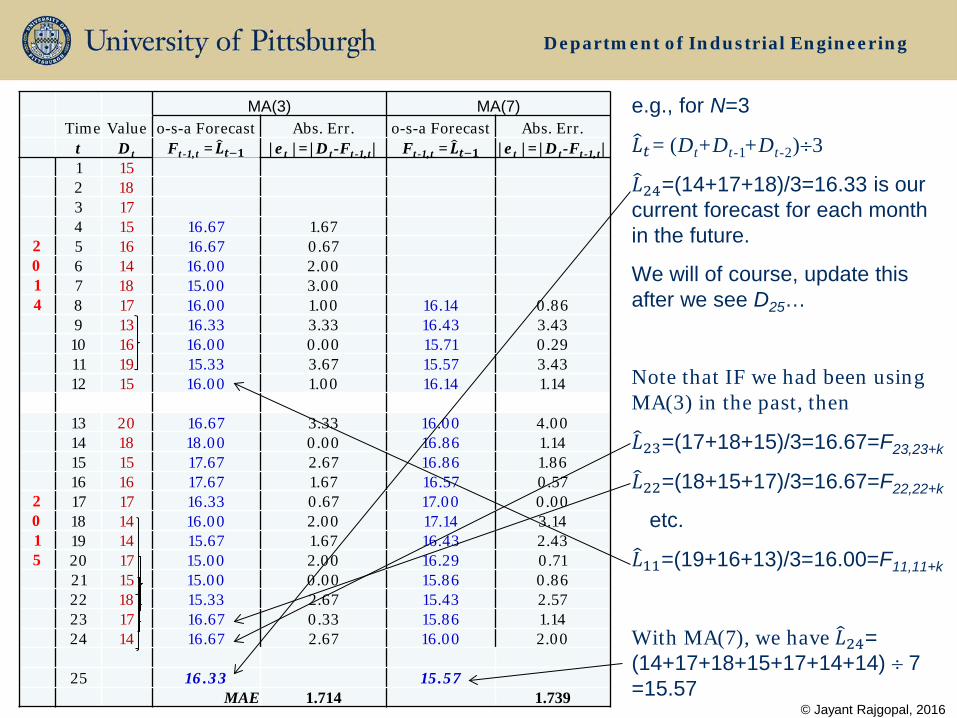
e.g., for N=3

𝐿�𝑡= (Dt+Dt-1+Dt-2)÷3

𝐿�24=(14+17+18)/3=16.33 is our current forecast for each month in the future.

We will of course, update this after we see D25…

Note that IF we had been using MA(3) in the past, then

𝐿�23=(17+18+15)/3=16.67=F23,23+k

𝐿�22=(18+15+17)/3=16.67=F22,22+k

etc.

𝐿�11=(19+16+13)/3=16.00=F11,11+k

With MA(7), we have 𝐿�24= (14+17+18+15+17+14+14) ÷ 7 =15.57

MA(3) MA(7) Time Value o-s-a Forecast Abs. Err. o-s-a Forecast Abs. Err. t Dt Ft-1,t =𝑳�𝒕−𝟏 |et |=|Dt-Ft-1,t| Ft-1,t =𝑳�𝒕−𝟏 |et |=|Dt-Ft-1,t| 1 15 2 18 3 17 4 15 16.67 1.67

2 5 16 16.67 0.67 0 6 14 16.00 2.00 1 7 18 15.00 3.00 4 8 17 16.00 1.00 16.14 0.86 9 13 16.33 3.33 16.43 3.43 10 16 16.00 0.00 15.71 0.29 11 19 15.33 3.67 15.57 3.43 12 15 16.00 1.00 16.14 1.14 13 20 16.67 3.33 16.00 4.00 14 18 18.00 0.00 16.86 1.14 15 15 17.67 2.67 16.86 1.86 16 16 17.67 1.67 16.57 0.57 2 17 17 16.33 0.67 17.00 0.00 0 18 14 16.00 2.00 17.14 3.14 1 19 14 15.67 1.67 16.43 2.43 5 20 17 15.00 2.00 16.29 0.71

21 15 15.00 0.00 15.86 0.86 22 18 15.33 2.67 15.43 2.57 23 17 16.67 0.33 15.86 1.14 24 14 16.67 2.67 16.00 2.00 25 16.33 15.57

MAE 1.714 1.739 © Jayant Rajgopal, 2016


Forecasting with Moving Averages


12

13

14

15

16

17

18

19

20

21

0 5 10 15 20 25

Time

Dem

and/

Fore

cast

Actual Values (Dt) O-S-A Forecast MA(3) O-S-A Forecast MA(7)


A good value for N might be something between 3 and 10

• Note that 𝐿�𝑡 = 1𝑁𝐷𝑡 + 𝐷𝑡−1 + ⋯+ 𝐷𝑡−(𝑁−1)

– So, as N increases we consider more data but give less weight to each individual data point – this smooths out fluctuations better

– Smaller values of N emphasize only recent data and give these more weight; it will therefore pick up any changes in the level more quickly

• Depending on the data, pick some candidate values for N. Then “pretend” that the model had been in use in the past and simulate on old data to see how each one performs before picking one



METHOD 2: Updating via Exponential Smoothing

We use the following formula to update the estimate of the level:

𝐿�𝑡 = 𝐿�𝑡−1 + α(Dt – 𝐿�𝑡−1) = 𝐿�𝑡−1 + α(Dt – Ft-1,t)

Note that

• If Dt – Ft-1,t >0, i.e., Ft-1,t < Dt then we are under-forecasting; so we apply a positive correction to our previous estimate

• If Dt – Ft-1,t< 0, i.e., Ft-1,t > Dt then we are over-forecasting; so we apply a negative correction to our previous estimate

Our previous estimate

“correction” based upon what we just observed



Here α is called a smoothing constant; larger values provide a bigger “correction” based on what just happened

We may also rearrange the formula to its more common form:

𝐿�𝑡 = 𝐿�𝑡−1 + α(Dt – 𝐿�𝑡−1) = Ft-1,t+ α(Dt – Ft-1,t)

= αDt + (1-α) 𝐿�𝑡−1 = αDt + (1-α) Ft-1,t

i.e., a weighted average of (1) what we just saw and (2) our forecast of what we thought we would see



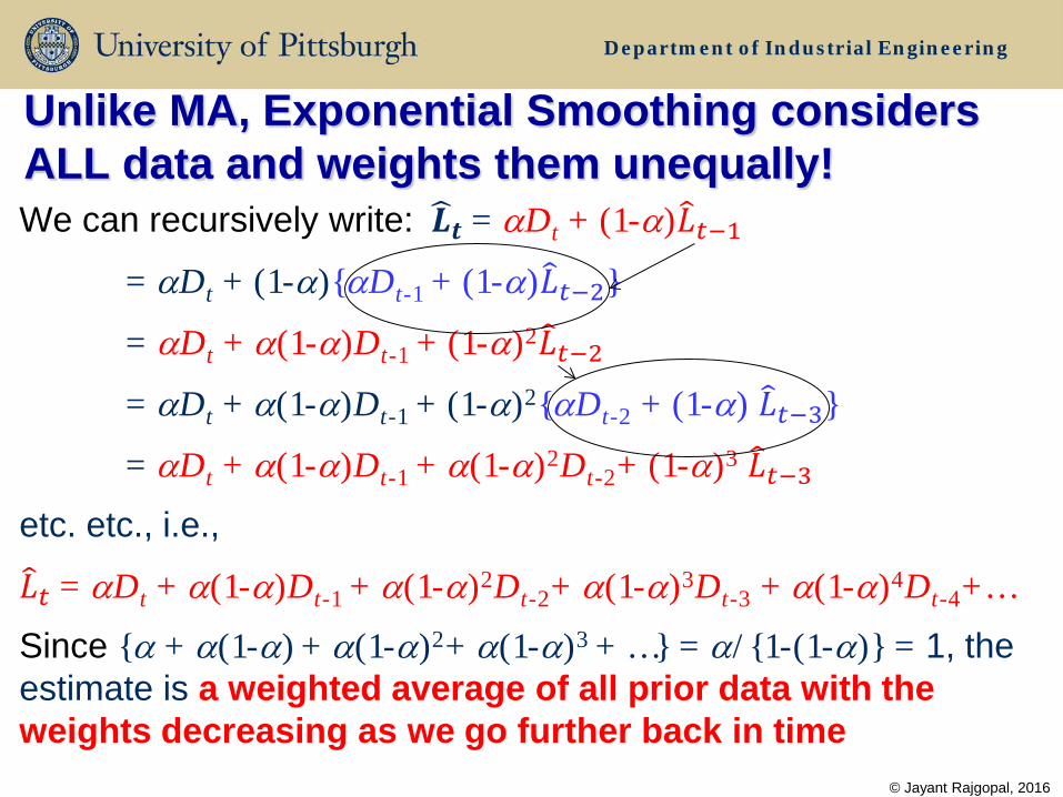
Unlike MA, Exponential Smoothing considers ALL data and weights them unequally! We can recursively write: 𝑳�𝒕 = αDt + (1-α)𝐿�𝑡−1

= αDt + (1-α){αDt-1 + (1-α)𝐿�𝑡−2}

= αDt + α(1-α)Dt-1 + (1-α)2𝐿�𝑡−2

= αDt + α(1-α)Dt-1 + (1-α)2{αDt-2 + (1-α) 𝐿�𝑡−3}

= αDt + α(1-α)Dt-1 + α(1-α)2Dt-2+ (1-α)3 𝐿�𝑡−3

etc. etc., i.e.,

𝐿�𝑡 = αDt + α(1-α)Dt-1 + α(1-α)2Dt-2+ α(1-α)3Dt-3 + α(1-α)4Dt-4+…

Since {α + α(1-α) + α(1-α)2+ α(1-α)3 + …} = α/{1-(1-α)} = 1, the

estimate is a weighted average of all prior data with the weights decreasing as we go further back in time



Consider the same example


13

14

15

16

17

18

19

20

0 4 8 12 16 20 24

Dem

and

Time

Time Value

t Dt 1 15 2 18 3 17 4 15

2 5 16 0 6 14 1 7 18 4 8 17 9 13 10 16 11 19 12 15 13 20 14 18 15 15 16 16 2 17 17 0 18 14 1 19 14 5 20 17

21 15 22 18 23 17 24 14 25


Assume α=0.1.

𝐿�𝑡=αDt+(1-α)𝐿�𝑡−1=αDt+(1-α)Ft-1,t

𝐿�24=0.1*14 + 0.9*16.18 = 15.96 is our current forecast for each month in the future = F24,24+k

We will of course, update this after we see D25…

Note that

𝐿�23=0.1*17 + 0.9*16.09 = 16.18

𝐿�22=0.1*18 + 0.9*15.88 = 16.09

𝐿�21=0.1*15 + 0.9*15.97 = 15.88

etc.

𝐿�12=0.1*15 + 0.9*15.87 = 15.78

etc.

Time Value O-S-A Forecast Abs. Err.

t Dt Ft-1,t = 𝑳�𝒕−𝟏 |et |=|Dt-Ft-1,t| 1 15 2 18 15.00 3.00 3 17 15.30 1.70 4 15 15.47 0.47

2 5 16 15.42 0.58 0 6 14 15.48 1.48 1 7 18 15.33 2.67 4 8 17 15.60 1.40 9 13 15.74 2.74 10 16 15.47 0.53 11 19 15.52 3.48 12 15 15.87 0.87 13 20 15.78 4.22 14 18 16.20 1.80 15 15 16.38 1.38 16 16 16.24 0.24 2 17 17 16.22 0.78 0 18 14 16.30 2.30 1 19 14 16.07 2.07 5 20 17 15.86 1.14

21 15 15.97 0.97 22 18 15.88 2.12 23 17 16.09 0.91 24 14 16.18 2.18 25 15.96

MAE 1.697 © Jayant Rajgopal, 2016


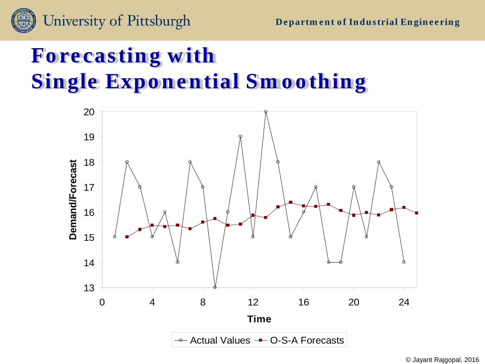
Forecasting with Single Exponential Smoothing


13

14

15

16

17

18

19

20

0 4 8 12 16 20 24

Time

Dem

and/

Fore

cast

Actual Values O-S-A Forecasts


Smaller α values provide better smoothing; larger values are more responsive

𝐿�𝑡= αDt + (1-α) 𝐿�𝑡−1

• Larger α implies more weight to Dt (i.e., to what happened recently – catches changes in the level quickly)

• Smaller α implies more weight to 𝐿�𝑡−1(i.e., to what has been happening in the past – smoother and less “jumpy”)


What just happened What we thought would happen based upon information from all previous data)

larger α may be better

smaller α may be better


A suggested range for α is [0.05, 0.30]

• Use a combination of subjective and objective evaluations to pick a final value

• Objective: – “Pretend” the model had been in use in the past and simulate

on old data with different α values to see how it performs.

• Subjective: – Does the data seem largely random

• If so, prefer a smaller value

– Does the data seem to have sudden level changes • If so prefer a larger value



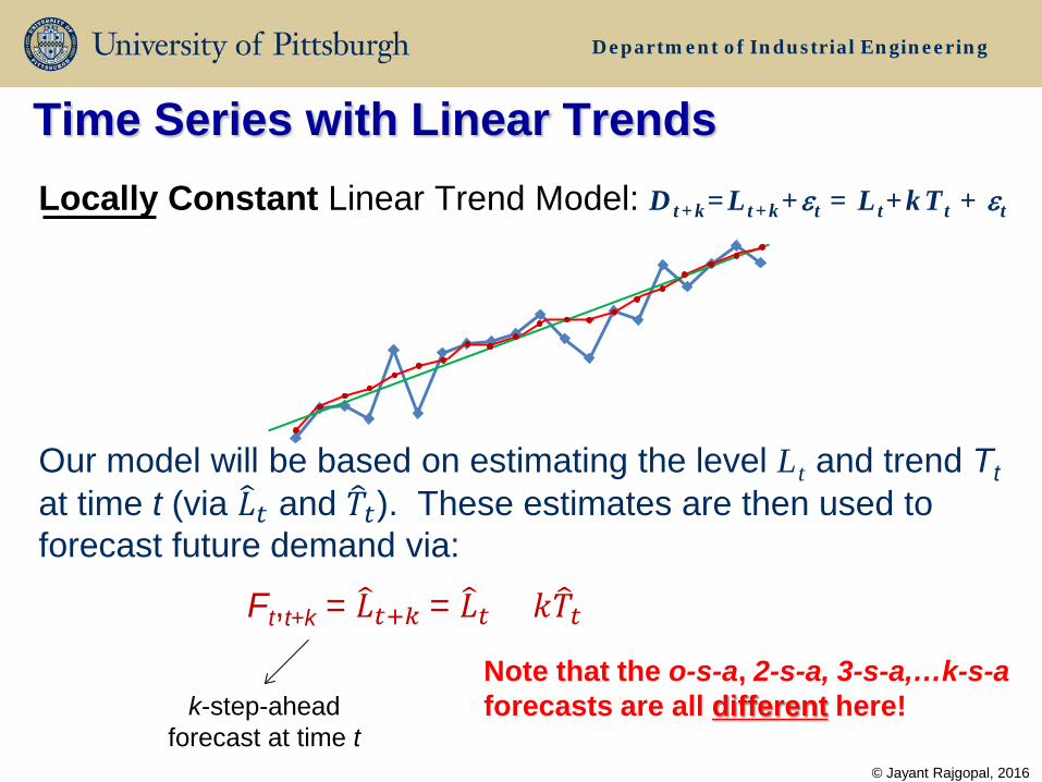
Locally Constant Linear Trend Model: Dt+k=Lt+k+εt = Lt+kTt + εt

Our model will be based on estimating the level Lt and trend Tt at time t (via 𝐿�𝑡 and 𝑇�𝑡). These estimates are then used to forecast future demand via:

Ft,t+k = 𝐿�𝑡+𝑘 = 𝐿�𝑡 + 𝑘𝑇�𝑡

Time Series with Linear Trends


k-step-ahead forecast at time t

Note that the o-s-a, 2-s-a, 3-s-a,…k-s-a forecasts are all different here!


Dt-2 Dt-1 Dt Ft,t+1 Ft,t+2 Ft,t+3 Ft,t+4

Visual representation:


End of time t: Ft,t+1= 𝐿�𝑡+𝑇�𝑡, Ft,t+2= 𝐿�𝑡+2𝑇�𝑡, Ft,t+3= 𝐿�𝑡+3𝑇�𝑡…

t-2 t-1 t t+1 t+2 t+3 t+4

Dt-2 Dt-1 Dt Dt+1 Ft+1,t+2 Ft+1,t+3 Ft+1,t+4

End of time t+1: Ft+1,t+2= 𝐿�𝑡+1+𝑇�𝑡+1, Ft+1,t+3= 𝐿�𝑡+1+2𝑇�𝑡+1, Ft+1,t+4= 𝐿�𝑡+1+3𝑇�𝑡+1…

t-2 t-1 t t+1 t+2 t+3 t+4

Dt-2 Dt-1 Dt Dt+1 Dt+2 Ft+2,t+3 Ft+2,t+4


t-2 t-1 t t+1 t+2 t+3 t+4

Dt-2 Dt-1 Dt Dt+1 Dt+2 Dt+3 Ft+3,t+4


t-2 t-1 t t+1 t+2 t+3 t+4


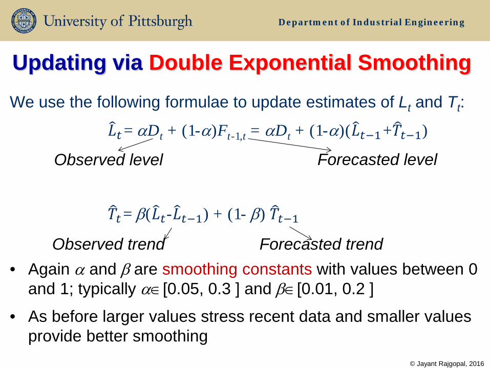
Updating via Double Exponential Smoothing We use the following formulae to update estimates of Lt and Tt:

𝐿�𝑡= αDt + (1-α)Ft-1,t = αDt + (1-α)(𝐿�𝑡−1+𝑇�𝑡−1)

𝑇�𝑡= β(𝐿�𝑡-𝐿�𝑡−1) + (1- β) 𝑇�𝑡−1

• Again α and β are smoothing constants with values between 0 and 1; typically α∈[0.05, 0.3 ] and β∈[0.01, 0.2 ]

• As before larger values stress recent data and smaller values provide better smoothing


Observed level Forecasted level

Observed trend Forecasted trend


Example


Time Value t Dt

1 98 2 94 3 99 4 104 5 108 6 100 7 106 8 104 9 118 10 109 11 102 12 116

13 115 14 120 15 126 16 123 17 120 18 128 19 136 20 128 21 126 22 134 23 140 24 135

25


Smoothing constants α=0.3 and β=0.1

Initialization: Regression through first 6 points yields an intercept c=94.8 and a slope m=1.629. Thus, estimates of mean level and trend at time t=6 are: 𝐿�6 = 94.8+6*1.629 = 104.574 and 𝑇�6 = 1.629 .

𝐿�𝑡= αDt+(1-α)Ft-1,t; 𝑇�𝑡= β(𝐿�𝑡-𝐿�𝑡−1)+(1- β) 𝑇�𝑡−1

Note that

𝐿�7=0.3*106 + 0.7*106.203 = 106.142

𝑇�7=0.1*(106.142 -104.574) + 0.9*1.629 = 1.623

𝐿�8=0.3*104 + 0.7*107.765 = 106.636

𝑇�8=0.1*(106.636 -106.142) + 0.9*1.623 = 1.510

etc…….

𝐿�23=0.3*140 + 0.7*134.734 = 136.314

𝑇�23=0.1*(136.314 -132.977) + 0.9*1.758 = 1.916

𝐿�24=0.3*135 + 0.7*138.23 = 137.261

𝑇�24=0.1*(137.261-136.314) + 0.9*1.916 = 1.819

These will be used to forecast each month in the future via F24,24+k = 137.261 + k(1.819)

Time Value O-S-A Forecast Abs. Err. Mean Trend

t Dt Ft-1,t = 𝑳�𝒕−𝟏+𝑻�𝒕−𝟏 |et |=|Dt-Ft| 𝑳�𝒕 𝑻�𝒕

1 98 2 94 3 99 4 104 5 108 6 100 104.574 1.629 7 106 106.203 0.203 106.142 1.623 8 104 107.765 3.765 106.636 1.510 9 118 108.145 9.855 111.102 1.806 10 109 112.907 3.907 111.735 1.688 11 102 113.424 11.424 109.996 1.346 12 116 111.342 4.658 112.740 1.485

13 115 114.225 0.775 114.457 1.509 14 120 115.966 4.034 117.176 1.630 15 126 118.806 7.194 120.964 1.845 16 123 122.810 0.190 122.867 1.851 17 120 124.718 4.718 123.303 1.710 18 128 125.012 2.988 125.909 1.799 19 136 127.708 8.292 130.196 2.048 20 128 132.244 4.244 130.970 1.921 21 126 132.891 6.891 130.824 1.714 22 134 132.538 1.462 132.977 1.758 23 140 134.734 5.266 136.314 1.916 24 135 138.230 3.230 137.261 1.819

25 139.080 © Jayant Rajgopal, 2016



Forecasting with Double Exponential Smoothing

94.8

1.629

104.574


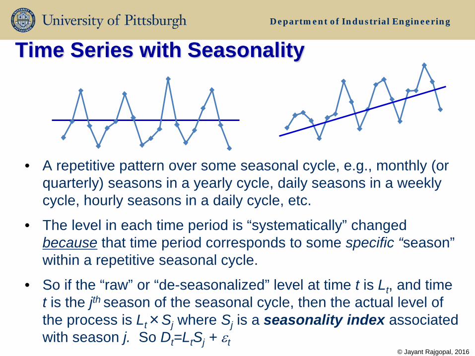
• A repetitive pattern over some seasonal cycle, e.g., monthly (or quarterly) seasons in a yearly cycle, daily seasons in a weekly cycle, hourly seasons in a daily cycle, etc.

• The level in each time period is “systematically” changed because that time period corresponds to some specific “season” within a repetitive seasonal cycle.

• So if the “raw” or “de-seasonalized” level at time t is Lt, and time t is the jth season of the seasonal cycle, then the actual level of the process is Lt×Sj where Sj is a seasonality index associated with season j. So Dt=LtSj + εt

Time Series with Seasonality



• Let N=No. of seasons in a seasonal cycle and Sj = seasonality index for season j, j=1,2,…,N

• The values of Sj are such that ∑jSj = N

The first step is to estimate the seasonality index Sj for each season j in the cycle


Time t Season j Dt CMAt Index Sj = Dt/CMAt

Week 1

1 2 3 4 5

Mon 4 Tue 7 Wed 9 8.4 1.071 Thu 14 8.2 1.710 Fri 8 7.8 1.026

Week 2

6 7 8 9

10

Mon 3 8.0 0.375 Tue 5 8.2 0.610 Wed 10 8.6 1.163 Thu 15 Fri 10

Thursday’s demand is 71% higher than “normal” because it is Thursday

Tuesday’s demand is 39% Lower than “normal” because it is Tuesday

etc.


1. Compute seasonality index values for each season using the centered-moving-average approach

2. De-seasonalize all data via Dt*=Dt/Sj (where j is the index of the season

corresponding to time t) – this “removes” the effect of the seasonality

3. Work on the de-seasonalized data Dt* as usual (i.e., single or double

exponential smoothing depending on whether or not a trend is present)

4. Build back the seasonality into the final forecast by multiplying the forecast by Sj where j is the index of the season corresponding to the time for which we are making the forecast: Ft,t+k = (F*

t,t+k)×Sj

The procedure follows four steps…



Example

Quarter Year 1 Year 2 Year 3 1 43 50 59 2 57 61 71 3 71 85 86 4 46 47 50

Consider the following quarterly data over three years



Find centered-moving-averages and then the seasonality indices Sj

t Quarter Demand 1 1 43 2 2 57 3 3 71 4 4 46 5 1 50 6 2 61 7 3 85 8 4 47 9 1 59 10 2 71 11 3 86 12 4 50


t Quarter C-M-A Sj=Dt/CMAt 1 1 2 2 3 3 55.125 1.288 4 4 56.500 0.814 5 1 58.750 0.851 6 2 60.625 1.006 7 3 61.875 1.374 8 4 64.250 0.732 9 1 65.625 0.899 10 2 66.125 1.074 11 3 12 4

Quarter 1 0.8751 0.871 Quarter 2 1.0400 1.035 Quarter 3 1.3309 1.325 Quarter 4 0.7728 0.769

SUM= 4.0187 4.000

Averaging multiple estimates and normalizing to ensure that they add up to 4.00, we get the final index estimates:

Note that with an even no. of seasons in the cycle (=4) we have to do our centering more carefully… 55.125 = {57+71+46+0.5(43+50)}÷4, 56.500 = {71+46+50+0.5(57+61)}÷4 etc. etc.


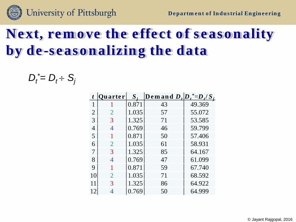
Next, remove the effect of seasonality by de-seasonalizing the data

t Quarter Sj Demand Dt Dt*=Dt/Sj

1 1 0.871 43 49.369 2 2 1.035 57 55.072 3 3 1.325 71 53.585 4 4 0.769 46 59.799 5 1 0.871 50 57.406 6 2 1.035 61 58.931 7 3 1.325 85 64.167 8 4 0.769 47 61.099 9 1 0.871 59 67.740

10 2 1.035 71 68.592 11 3 1.325 86 64.922 12 4 0.769 50 64.999


Dt*= Dt ÷ Sj


Note how the seasonal swings are gone, and an increasing trend seems to be present


40

50

60

70

80

90

100

0 2 4 6 8 10 12

Valu

es/F

orec

asts

Time

Actual Values Deseasonalized Values


Now use double exponential smoothing on the de-seasonalized data

t Quarter Dt*=Dt/Sj F*

t-1,t 𝑳�𝒕* 𝑻�𝒕* 1 1 49.370 2 2 55.066 3 3 53.598 53.598 2.142 4 4 59.799 55.740 56.552 2.223 5 1 57.406 58.775 58.501 2.196 6 2 58.931 60.697 60.344 2.160 7 3 64.167 62.504 62.837 2.194 8 4 61.099 65.031 64.244 2.115 9 1 67.740 66.359 66.635 2.143

10 2 68.592 68.778 68.741 2.139 11 3 64.922 70.880 69.688 2.020 12 4 64.999 71.708 70.366 1.886 13 1 72.252


Smoothing constants α=0.2 and β=0.1

Initialization: An approximate trend line was obtained by “eyeballing” the data. Specifically, the line chosen passed through D3

* and D10* as

displayed on the graph. Corresponding to this line we have .

𝐿�3∗=D3*=53.598, and

𝑇�3* = (D10*- D3

*)÷(10-3)

= (68.592-53.598)/7 = 2.142

Now update as usual starting with t=4…

At the end of t=12, we get the current estimates of level and trend:

𝐿�12∗ =70.366, and 𝑇�12∗ = 1.866


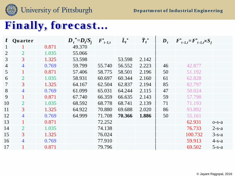
Finally, forecast… t Quarter Dt

*=Dt/Sj F*t-1,t 𝑳�𝒕* 𝑻�𝒕* Dt F*

t-1,t=F*t-1,t×Sj

1 1 0.871 49.370 2 2 1.035 55.066 3 3 1.325 53.598 53.598 2.142 4 4 0.769 59.799 55.740 56.552 2.223 46 42.877 5 1 0.871 57.406 58.775 58.501 2.196 50 51.192 6 2 1.035 58.931 60.697 60.344 2.160 61 62.828 7 3 1.325 64.167 62.504 62.837 2.194 85 82.797 8 4 0.769 61.099 65.031 64.244 2.115 47 50.024 9 1 0.871 67.740 66.359 66.635 2.143 59 57.798 10 2 1.035 68.592 68.778 68.741 2.139 71 71.193 11 3 1.325 64.922 70.880 69.688 2.020 86 93.892 12 4 0.769 64.999 71.708 70.366 1.886 50 55.161 13 1 0.871 72.252 62.931 o-s-a 14 2 1.035 74.138 76.733 2-s-a 15 3 1.325 76.024 100.732 3-s-a 16 4 0.769 77.910 59.913 4-s-a 17 1 0.871 79.796 69.502 5-s-a



Seems to be working quite well…



Forecasts should be assessed w.r.t. accuracy and bias Given errors e1, e2,…eN

• Mean error = (∑jej)/N (…should be close to zero if unbiased)

• Mean Absolute Deviation = MAD = (∑j|ej|)/N (…should be small)

• Mean Squared Error = MSE = (∑j(ej)2)/N (…should be small)

• Mean Absolute Percentage Error=MAPE= 100*(∑j|ej/Dj|)/N (…should be small)

Often instead of just taking raw error averages, we might choose to smooth the errors (or functions of the error):

• Smoothed mean error Et= ω(et) + (1-ω)Et-1 (should eventually be close to zero)

• Smoothed Mean Absolute Deviation MADt = ω(|et|) + (1-ω)(MADt-1).

• Tracking Signal = Et/MADt (close to zero if the forecasts are unbiased)

• Average % error = MAD/Forecast



Assume α=0.3 and β=0.1 and suppose we had initial estimates at the end of t=3 of 𝐿�3 =59.075 and 𝑇�3 =3.166

t Dt Ft 𝐿�𝑡 𝑇�𝑡 et Et |et| MADt |Et ÷

MADt| 1 20 2 31 3 50 (59.075) (3.166) 4 59 62.241 61.269 3.069 -3.241 3.241 5 60 64.338 63.036 2.939 -4.338 -3.351 4.338 3.351 1.000 6 62 65.975 64.782 2.819 -3.975 -3.413 3.975 3.413 1.000 7 65 67.602 66.821 2.741 -2.602 -3.332 2.602 3.332 1.000 8 74 69.563 70.894 2.874 4.437 -2.555 4.437 3.443 0.742 9 75 73.768 74.138 2.911 1.232 -2.176 1.232 3.221 0.676

10 80 77.049 77.934 3.000 2.951 -1.664 2.951 3.194 0.521 11 83 80.934 81.554 3.062 2.066 -1.291 2.066 3.082 0.419 12 88 84.616 85.631 3.163 3.384 -0.823 3.384 3.112 0.265 13 92 88.795 89.756 3.260 3.205 -0.420 3.205 3.121 0.135 14 95 93.016 93.611 3.319 1.984 -0.180 1.984 3.007 0.060 15 101 96.930 98.151 3.441 4.070 0.245 4.070 3.114 0.079 16 101 101.592 101.415 3.423 -0.592 0.161 0.592 2.862 0.056 17 106 104.838 105.187 3.458 1.162 0.261 1.162 2.692 0.097 18 108 108.645 108.451 3.439 -0.645 0.171 0.645 2.487 0.069 19 112 111.890 111.923 3.442 0.110 0.165 0.110 2.249 0.073 20 109 115.366 113.456 3.251 -6.366 -0.488 6.366 2.661 0.184 21 114 116.707 115.895 3.170 -2.707 -0.710 2.707 2.665 0.266 22 118 119.065 118.746 3.138 -1.065 -0.746 1.065 2.505 0.298 23 121 121.884 121.619 3.112 -0.884 -0.760 0.884 2.343 0.324 24 125 124.730 124.811 3.120 0.270 -0.657 0.270 2.136 0.307 25 127.931

Average = -0.074 2.442



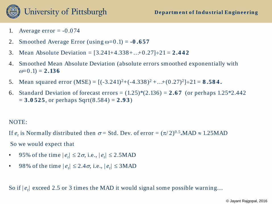
1. Average error = -0.074

2. Smoothed Average Error (using ω=0.1) = -0.657

3. Mean Absolute Deviation = [3.241+4.338+…+0.27]÷21 = 2.442

4. Smoothed Mean Absolute Deviation (absolute errors smoothed exponentially with ω=0.1) = 2.136

5. Mean squared error (MSE) = [(-3.241)2+(-4.338)2 +…+(0.27)2]÷21 = 8.584.

6. Standard Deviation of forecast errors = (1.25)*(2.136) = 2.67 (or perhaps 1.25*2.442 = 3.0525, or perhaps Sqrt(8.584) = 2.93)

NOTE:

If et is Normally distributed then σ = Std. Dev. of error = (π/2)0.5*MAD ≈ 1.25MAD

So we would expect that

• 95% of the time |et| ≤ 2σ, i.e., |et| ≤ 2.5MAD

• 98% of the time |et| ≤ 2.4σ, i.e., |et| ≤ 3MAD

So if |et| exceed 2.5 or 3 times the MAD it would signal some possible warning…


forecasting: the first step in demand planningjrclass/sca/notes/2-forecasting.pdf · forecasting:...

Documents