Economic Modernization through Efficient Reforms and Governance Enhancement (EMERGE) Unit 2003, 139 Corporate Center, 139 Valero St., Salcedo Village, Makati City 1227, Philippines

Tel. No. (632) 752 0881 Fax No. (632) 752 2225

Technical Report

Forecasting Revenues from the BIR and BOC: Towards the Improvement of Cash Programming in the Philippines by Joselito R. Armovit

Prepared for Department of Budget and Management Republic of the Philippines Submitted for review to USAID/Philippines OEDG

September 23, 2005

Preface

This report is the result of technical assistance provided by the Economic Modernization through Efficient Reforms and Governance Enhancement (EMERGE) Activity, under contract with the CARANA Corporation, Nathan Associates Inc. and The Peoples Group (TRG) to the United States Agency for International Development, Manila, Philippines (USAID/Philippines) (Contract No. AFP-I-00-00-03-00020 Delivery Order 800). The EMERGE Activity is intended to contribute towards the Government of the Republic of the Philippines (GRP) Medium Term Philippine Development Plan (MTPDP) and USAID/Philippines’ Strategic Objective 2, “Investment Climate Less Constrained by Corruption and Poor Governance.” The purpose of the activity is to provide technical assistance to support economic policy reforms that will cause sustainable economic growth and enhance the competitiveness of the Philippine economy by augmenting the efforts of Philippine pro-reform partners and stakeholders. This technical report was completed by Joselito R. Armovit in September 2005. The technical assistance was requested by Department of Budget and Management (DBM) Undersecretary Laura B. Pascua in a letter dated March 29, 2005. The views expressed and opinions contained in this publication are those of the authors and are not necessarily those of USAID, the GRP, EMERGE or the latter's parent organizations.

Forecasting Revenues from the BIR and BoC: Towards the Improvement of Cash

Programming in the Philippines

Joselito R. Armovit

23 September 2005

TABLE OF CONTENTS Abstract.....................................................................................................................................2 I. Introduction .........................................................................................................................3

The MTEF and the Need for “Honest” Revenue Projections ............................................3 Revenues, Disbursements and Monthly Deficits ...............................................................4

II. Public Revenues: Targets versus Forecasts.....................................................................5 Forecasting Methods..........................................................................................................6 Public Revenues in the Philippines....................................................................................6

III. Taxes from the Bureau of Internal Revenue .................................................................7 A) Profiling Collections from the BIR..................................................................................7

Tax Types...........................................................................................................................7 Schedule of Payments ........................................................................................................8

B) Forecasting BIR Collections ..........................................................................................12 Random Walk ..................................................................................................................12 Actual BIR Collections versus Forecasts for 2004 ..........................................................12

IV. Revenues form the Bureau of Customs ........................................................................14 A) Profiling Collections from the BoC...............................................................................14

Duties and Taxes..............................................................................................................14 B) Forecasting BoC Collections .........................................................................................16

The Effective Rate and the Tariff Rate ............................................................................17 Actual BoC Collections versus Forecasts for 2004 .........................................................18

V. Conclusion.........................................................................................................................19 References ...............................................................................................................................20 Appendix A .............................................................................................................................21 Appendix B .............................................................................................................................23

1

Forecasting Revenues from the BIR and BoC: Towards the Improvement of Cash Programming in the Philippines

Abstract This paper introduces a methodology for forecasting revenues collected by both Bureaus of Internal Revenue and Customs, together making up about 99% of tax revenues, and about 87% of total National Government revenues. A distinction is made between forecasting, and target setting. While the latter reflects a desired level of revenues based on the medium term fiscal program, the former is based on a more realistic appreciation of current trends and capacities of the revenue Bureaus, and the taxpaying public, for programming budget releases. The need to predict revenue inflows by the Department of Budget and Management is brought about by the need to ensure a more stable and predictable program of cash allotments to agencies throughout the year to engender an environment for greater results orientation. Once established this, and the effort to measure outputs in government, will eventually serve as an input to the plan to establish a Medium Term Expenditure Framework for the Philippines within the next few years. While the importance of planning public expenditure for a medium term is important for stability and transparency, the predictability of revenues is a key element in that it builds credibility and ensures the sustainability of the program.

2

I. Introduction The purpose of this paper is to introduce an alternative methodology (or methodologies) for systematically forecasting government revenues in the Philippines using monthly trends. The need to predict revenue inflows by the Department of Budget and Management is brought about by the need to ensure a more stable and predictable program of fund releases to implementing agencies throughout the year, in a way that reduces the risk of breaching the quarterly or monthly deficit target. And for the medium term, the predictability of public revenues will be a key element to the Philippine government’s plan set in place, a focus towards results, and to establish a medium term expenditure framework, or MTEF, within the next few years. While it is beyond the purview of this report to discuss exhaustively the concept of an MTEF, its merits, nor the obstacles leading to its proper implementation, a brief introduction is important. The MTEF and the Need for “Honest” Revenue Projections The MTEF is a framework that puts in place a longer term public expenditure program, usually a 3 year expenditure cycle1, which allows the government to support a strategic and policy based approach to budget preparation. But why a longer term horizon for public expenditures, when the national government will have to go to congress each year to have its budget approved anyway, with or without an MTEF? The first reason is to enhance stability. If government agencies are aware beforehand of how much resources will be available to them for the next 3 years, then planning will be better thought out and therefore more accurate and credible. Next, it improves transparency. An MTEF signals to the public, the government’s priorities and how it intends to implement its vision within the next 3 years. And in so doing, it may encourage greater public debate on its goals. Lastly, an MTEF may encourage more investments since it makes public spending more predictable. And playing a central role to the sustainability of any MTEF therefore, is the predictability of current as well as future stream of government revenue inflows.

1 Presentation documents and articles from the World Bank website archives usually mention 3 years for an

MTEF.

3

Revenues, Disbursements and Monthly Deficits In the Philippines, the close link between the revenue and expenditure programs of the government is revealed in the outcome of actual monthly deficits, as they differ from the monthly deficit targets. At the beginning of each year, the government programs the country’s monthly deficit ceiling to be consistent with the annual deficit target. The programmed ceiling in each month is the difference between the projected revenue and the programmed disbursement of the government for the same month, calculated at the beginning of the year. Recent records show that the programmed monthly target usually varies from the actual monthly deficit reached. Figure 1. Monthly Deficits: Actual versus Program

(30,000)

(25,000)

(20,000)

(15,000)

(10,000)

(5,000)

-

5,000

10,000

15,000

Jan

Feb

Mar

Apr

May Jun

Jul

Aug Sep Oct

Nov

Dec Jan

Feb

Mar

Apr

May Jun

Jul

Aug Sep Oct

Nov

Dec Jan

Feb

Mar

Apr

May Jun

Jul

Aug Sep Oct

Nov

Dec

2001 2002 2003

Program Actual

During the years 2001, 2002 and 2003, the programmed monthly deficit was different from the actual levels. For the latter 2 years, this resulted in two very different scenarios. In 2002, as actual levels consistently surpassed (larger deficits) programmed levels, the cumulative deficit towards the first half of the year showed a worsening fiscal scenario. This scene was completely reversed in 2003. Continuous improvements in actual monthly deficits resulted in a more favorable fiscal scene by the end of the first half (see figures 2-A and 2-B below). The uncertainty in the monthly and even quarterly fiscal scenario, as actual deficits vary from programmed levels, can be traced to the volatility of both revenues and disbursements. Estimates may show that in 2002, the volatility of disbursements was slightly larger than that of revenues2. However, it should be noted that actual disbursements are in part based on projected revenues. The latter ideally acts as a ceiling to the amount of actual disbursements. Viewed this way, the volatility in disbursements therefore is also driven by the volatility of revenue generation. 2 The standard deviation of the percentage difference between actual and programmed levels in 2002 are 8.23

for disbursements and 7.49 for revenues.

4

Figure 2-A. Cumulative Deficit: 2002 Figure 2-B. Cumulative Deficit: 2003

(120 ,000 )

(100 ,000 )

(80 ,000 )

(60 ,000 )

(40 ,000 )

(20 ,000 )

-

J a n F e b M a r A p r M a y Ju n

2 0 0 3

P ro g ra m A c tu a l

(140,000)

(120,000)

(100,000)

(80,000)

(60,000)

(40,000)

(20,000)

-

Jan Feb Mar Apr May Jun

2002

Program Actual

As actual deficits continue to differ from programmed levels, there are two things that government may do. If allowed, it may choose to adjust the yearend deficit target, or, it may instead adjust future disbursements to be consistent with the yearend deficit target. A third option, if available, is to adjust the revenue target upward in the event that the actual cumulative deficit is higher than the programmed level. One way to do this is for the national government to impose discretionary revenue measures on its collecting agencies. II. Public Revenues: Targets versus Forecasts For the purpose of this paper3, a revenue target may be differentiated from a revenue forecast by the amount of discretionary revenue measures anticipated at the beginning of a fiscal period.

Revenue Target = Revenue Forecast + Discretionary Measures A target therefore is the sum of the forecast plus anticipated revenues from administrative and/or legislative measures aimed at increasing collections. While a revenue target represents a desired level, a forecast on the other hand represents a realistic level of revenues that is generated using available (tax) systems, current levels of collection efficiency as well as the revenue base that is available for the government to collect from. A forecast, therefore, can be calculated using past revenue collections as they reflect the conditions mentioned above. If the level of the forecast is less than what is desired, then government may present discretionary measures to augment it. Such is the case of the EVAT law passed earlier this year, and the “sin” tax law in 2004 allowing the indexation of sin taxes to inflation.

3 Golosov (2002) shows that many countries often interchange the terms “targets”, “forecasts” and

“projections”. In practice, targets are commonly set high either to encourage additional efforts from collectors or to showcase expected macroeconomic gains. Thus, a distinction must be made.

5

Forecasting Methods There are two ways in which revenue forecasting is normally practiced: First, the forecast may be calculated as an unconditional prediction of the most likely outcome. And second, a forecast may be performed conditionally on the accuracy of macroeconomic variables that are used as a basis for the prediction. In a study by the IMF, using a sample of 34 countries from Africa, Asia, Latin America and the Middle East, they show that although not all of the countries rely on macroeconomic forecasts as inputs to the revenue forecast, majority still do4. While 85% of the sampled countries use subjective assessment and basic extrapolation techniques as their main forecasting methodology, only about 13% use formal econometric methods. And between 75 – 80% calculate their forecasts using aggregate revenue data. In order to accurately isolate the impact of discretionary measures from nominal collections, some authors prefer to estimate a built-in tax elasticity model5. Although there are a number of ways to do this, their objective is the same, and that is to measure the percentage increase in tax revenues that result from endogenous changes in the tax base, caused by a 1 percent rise in nominal GDP. The approach using tax elasticities to forecast revenues is also used in Ireland. The Department of Finance in Ireland, recommends a great deal of flexibility when performing tax revenue forecasts. Although their official method is a more elaborate econometric technique to forecast disaggregate tax data, the Tax Forecasting Methodology Group recommends a top-down macroeconomic test against the GDP:revenue trends, to supplement the forecasts.

“…reliance on a single approach to tax forecasting carried risks, and, that it needed to be tested against aggregate tax elasticities”6

Furthermore, the Group also shows that in recent years, the reason for the under-performance of Ireland’s revenue projections was mainly due to the over- performance of the economy, compared to GDP forecasts. Public Revenues in the Philippines In 2004, total public revenues generated by the government amounted to about P 685B of which: 4 Kyobe and Danniger ”Revenue Forecasting—How is it Done? …” IMF Working Paper, 2005. 5 Ehdaie, Jaber “An Econometric Method for Estimating the Tax Elasticity…” World Bank, February 1990. 6 Report of Tax Forecasting Methodology Group. Department of Finance, Ireland. 2005

6

Tax Revenues 87.3% BIR 68.3% BoC 17.9% Others 1.1%

Non-Tax Revenues 12.7%

Source: The Fiscal Planning Bureau,

Department of Budget and Management Revenues from the Bureau of Internal Revenue and the Bureau of Customs together make up about 86% of the total. While more than half (about 65%) of non-tax revenues were generated from the income of the Bureau of Treasury. The rest come from privatization proceeds, interest income of the Banko Sentral ng Pilipinas, foreign grants, etc. The difficulty in relying on any forecasting technique to predict the revenues of the BTr is highlighted by it recent performance where it exceeded its target by 22% and 84% in 2002 and 2003 respectively. And attempting to forecast all other revenues, which are of different natures, would require a tedious and elaborate process disproportionate to their actual contribution to the revenue pie. III. Taxes from the Bureau of Internal Revenue A) Profiling Collections from the BIR Tax Types The Bureau of Internal Revenue collects five (5) major taxes. They are: income taxes, the value added tax, excise taxes, percentage taxes, and fixed taxes on business and other activities labeled as “other taxes” in government fiscal documents. These 5 major taxes are presented in more detail below. Table 1. Tax Types of the BIR

I. Tax on Net Income a. Company, corporate enterprise

i. Corporate ii. Withholding at source

b. Individual i. Individual ii. Withholding on wages iii. Capital gains iv. Withholding at source

c. Others (bank deposits/treasury bills)

II. Excise Tax a. Alcohol

7

b. Tobacco c. Petroleum d. Miscellaneous e. Mining/minerals

III. Value Added Tax IV. Percentage Taxes

a. Banks/financial institutions b. Insurance premiums c. Amusement d. Franchise tax e. Other percentage taxes

V. Other Taxes a. Transfer tax b. DST c. Travel tax d. Miscellaneous

Each major tax collected by the Bureau is affected by different factors. Net or taxable income for income taxes, volume of production for excisable products, net (“vat-able”) sales for VAT, and the value and volume of business activities for percentage and other taxes. Schedule of Payments Within a given year, however, the monthly fluctuations internal revenue generation is affected by tax deadlines given by the tax code. Figure 3. Trend of Monthly Collections, in Billion Pesos

10.00

20.00

30.00

40.00

50.00

J F M A M J J A S O N D J F M A M J J A S O N D J F M A M J J A S O N D J F M A M J J A S O N D J F M A M J J A S O N D J F M A M J J A S O N D J F M A M J J A S O N D J F M A M J J A S O N D J F M A M J J A S O N D J F M A M J J A S O N D

1995 1996 1997 1998 1999 2000 2001 2002 2003 2004

Thus for any given year, the typical distribution of collections can be presented in the graph below.

8

Figure 4. Average Monthly Distribution of BIR Revenues

8.32

6.397.11

11.45

8.46

7.407.98

8.91

7.15

8.10

9.49 9.23

4.00

6.00

8.00

10.00

12.00

Jan Feb Mar Apr May Jun Jul Aug Sep Oct Nov Dec

perc

enta

ge

In any year for the last 5 years (2000-2004)7, the monthly distribution of BIR collections tend to deviate by +/- 0.5 percentage point from the average. If years prior to 2000 were included, then the deviation from average would be even greater. The pronounced peaks occurring in April, May, August and November are due to the payment of income taxes for both corporations and individuals. Quarterly income taxes, which are paid 60 days after the end of a quarter, create the peaks for May, August and November. The fourth quarter of a taxpayer’s fiscal year, as well as any unpaid balances, are paid in April of the following year. The value added tax has a current statutory rate of 10%8. It is levied on a monthly basis, but is collected on the following month that the sales were generated. While the VAT as a whole is collected every month, quarterly payments are made on the following month for any remaining balances. On the whole and on average, excise taxes are collected each month. However, individual excise taxpayers, and in some occasions, certain industry groups have different payment schedules from each another. This is because the tax system, by law, imposes that no goods can be transferred out from production site to distribution outlets without the full payment of excise taxes. Thus practice has been that manufacturers will pay the tax in advance so not to create delays in delivery and sales schedules. Percentage and “other” taxes are collected on the following month that the taxable activities took place. On the whole, these taxes are also collected every month.

7 In pesos, the deviation from average is equivalent to about +/- P 2.0-2.5B each month. 8 The EVAT law of 2005 allows the VAT rate to be raised to 12% by the President if certain conditions are met.

The effective rate, however, is more often less than the statutory rate because the previous VAT payments in upstream linkages are deducted from what is due a taxpayer.

9

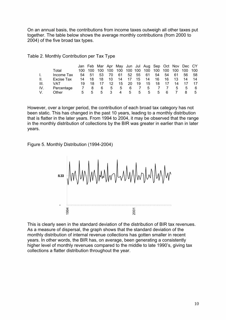
On an annual basis, the contributions from income taxes outweigh all other taxes put together. The table below shows the average monthly contributions (from 2000 to 2004) of the five broad tax types. Table 2. Monthly Contribution per Tax Type Jan Feb Mar Apr May Jun Jul Aug Sep Oct Nov Dec CY

Total 100 100 100 100 100 100 100 100 100 100 100 100 100 I. Income Tax 54 51 53 70 61 52 55 61 54 54 61 56 58 II. Excise Tax 14 18 18 10 14 17 15 14 16 16 13 14 14 III. VAT 19 18 17 12 15 20 19 15 18 17 14 17 17 IV. Percentage 7 8 6 5 5 6 7 5 7 7 5 5 6 V. Other 5 5 5 3 4 5 5 5 5 6 7 8 5

However, over a longer period, the contribution of each broad tax category has not been static. This has changed in the past 10 years, leading to a monthly distribution that is flatter in the later years. From 1994 to 2004, it may be observed that the range in the monthly distribution of collections by the BIR was greater in earlier than in later years. Figure 5. Monthly Distribution (1994-2004)

-

8.33

1994

2001

This is clearly seen in the standard deviation of the distribution of BIR tax revenues. As a measure of dispersal, the graph shows that the standard deviation of the monthly distribution of internal revenue collections has gotten smaller in recent years. In other words, the BIR has, on average, been generating a consistently higher level of monthly revenues compared to the middle to late 1990’s, giving tax collections a flatter distribution throughout the year.

10

Figure 6. Standard Deviation of Monthly Distribution

1.00

1.20

1.40

1.60

1.80

2.00

stdev 1.70 1.85 1.86 1.87 1.43 1.68 1.37 1.47 1.37 1.50 1.34

199 199 199 199 199 199 200 200 200 200 200

One reason for this was the expansion in the coverage of the VAT, which occurred in 1996 with the EVAT law. Other reasons include administrative improvements in the collections of VAT, such as the VAT Relief9. The VAT, as shown earlier, is paid on a monthly basis. Thus any increase in its performance has a tendency to flatten the monthly profile of tax collections as a whole. Data also shows that the monthly profile of income taxes have gotten flatter as well in recent years. This change may be administrative in nature10. And it seems to have evolved from a necessity on the expenditure side to have a steadier stream of revenues throughout the year, leading to stricter imposition of the quarterly income tax especially on corporations. Figure 7. Monthly Contribution of Income and VAT: 2000-2004 vs. 1997

-

10.00

20.00

30.00

40.00

50.00

60.00

70.00

80.00

Income ave 54.19 50.76 53.34 70.00 61.57 52.04 54.80 61.24 53.81 53.81 60.98 55.96 57.64

Income 97 47.79 44.15 44.97 71.74 54.48 50.62 43.36 61.27 48.20 44.56 49.06 53.22 52.55

VAT ave 19.21 18.32 17.32 11.85 15.12 19.93 18.75 15.53 18.50 17.49 14.42 17.56 16.71

VAT 97 21.04 16.34 17.89 7.36 11.62 17.44 19.92 11.83 16.69 16.73 14.80 13.33 14.91

Jan Feb Mar Apr May Jun Jul Aug Sep Oct Nov Dec CY

9 The VAT Relief is a system that electronically matches the sales data of firms with the tax declarations of

others. VAT due is then extrapolated. 10 It is the absence of a change in the rules that mandate a more dispersed collection of income tax through any

given year that convinces one that the change was administrative in nature.

11

B) Forecasting BIR Collections Random Walk A stochastic time series {yt} of the form, yt = µ + yt-1 + εt is a random walk, where εt is white noise11. A random walk can be described as a time series process wherein the direction of a random variable’s change, in the next period, is not completely known. In turn, and given complete information, the direction and magnitude of change is directly affected by new information as it unfolds. The random walk model is often used to explain movement in stock prices. The reason being that, in efficient markets, all the information needed by investors to make predictions on the direction of future stock prices is already reflected in the current price. That is, all existing information affects stock prices, which changes only as new information is revealed and in a random manner. In the Philippines internal revenue system, the taxes that one pays in a fiscal season form a stream of tax payments, where the amount of each is a consequence of that paid in previous periods. This is evident in the payment of income taxes and the VAT, together forming close to 80% of total taxes. While tax deadlines determine the trend in collections, the actual level of taxes paid by each individual taxpayer is dictated by several factors that affect his level of taxable income during the period, as well as expectations of future income streams. Weighing these factors together help to determine a taxpayer’s behavior. In the aggregate, while the monthly trend is clearly defined by codal deadlines, the actual levels (or deviations from what actually must be paid) are determined by several factors including previously unknown information that unfolds in the course of the fiscal year. Actual BIR Collections versus Forecasts for 2004 For purposes of comparison, four different models were used to forecast BIR revenues on a quarterly and monthly basis. These were then compared to each other, as well as compared to the actual levels of tax collections. The actual data used were total quarterly collections from 1990 to 2003, and monthly collections from 2000 to200312. These were then used to predict the quarterly and monthly aggregate collections for 2004.

11 E[εt] = 0; Var(εt) = σ2,a constant; Cov(εt, εt-s) = 0 for all s # 0 12 Many thanks to the BIR-Policy and Planning Office, the DOF-Fiscal Policy and Planning Office, the DBM-

Fiscal Planning Bureau, the BSP-Department of Economic Research, and the Philippine Institute for Development Studies for providing the data.

12

Table 3. Forecast versus Actual BIR Collections (I) (II) (III) (IV)

BIR=f(gdpn) BIR=g(gdpr, tb91) ARIMA (4,1,1) (4, 0)s

ARIMA (12,1,1)

MAPE 4.6556 MAPE 4.1061 MAPE 4.47136 MAPE 6.17737

(in million P) Actual (A) Forecasts

Q1 98,974.16 99,230.00 102,717.77 97,113.41 98,681.59 Q2 130,218.10 127,069.02 129,537.74 120,345.41 126,562.47 Q3 114,655.05 113,309.22 119,584.73 108,727.57 111,440.71 Q4 124,329.27 126,229.59 132,869.07 122,165.64 124,186.04

Total 04 468,176.58 465,837.83 484,709.32 448,352.03 460,870.81 With AdM* 468,176.58 471,012.83 489,884.32 453,527.03 466,045.81

(B) Deviation (Forecast less Actual)

Q1 - 255.84 3,743.61 (1,860.75) (292.57) Q2 - (3,149.08) (680.36) (9,872.69) (3,655.63) Q3 - (1,345.83) 4,929.68 (5,927.48) (3,214.35) Q4 - 1,900.32 8,539.80 (2,163.64) (143.23)

Total 04 - (2,338.75) 16,532.73 (19,824.55) (7,305.78) With AdM - 2,836.25 21,707.73 (14,649.55) (2,130.78)

(C) Deviation (in %)

Q1 - 0.26 3.78 (1.88) (0.30) Q2 - (2.42) (0.52) (7.58) (2.81) Q3 - (1.17) 4.30 (5.17) (2.80) Q4 - 1.53 6.87 (1.74) (0.12)

Total 04 - (0.50) 3.53 (4.23) (1.56) With AdM - 0.61 4.61 (2.99) (0.47)

*Targeted administrative measures were P 5,175M, as of 27 January 2004, for the same year. Four different models were used to forecast 2004 quarterly collections. The first three models used quarterly data from 1990 to 2003, while the last one used monthly actual collections from 2000 to 2003. The first estimated the tax elasticity, to nominal GDP. This measures the percentage increase in tax revenue that results from an endogenous change in the tax base, from a one percent rise in GDP. The second model assumes that the change in tax revenue is due to the change in real GDP and domestic interest rates. The third model is an ARIMA model, with a seasonal AR term for the quarterly data. The fourth is also an ARIMA model, but this time using monthly data (see Appendix A). The monthly output was then aggregated into quarterly collections in order to compare with the output of the other models. When comparing the results with actual collections in 2004, in order to assess the accuracy of the forecasts, we find that the most accurate forecast (i.e. with the lowest deviation from actual) is one calculated by the elasticity model (GDPn).

13

However, one must understand that at the beginning of the year, administrative measures amounting to P 5,175M were also imposed on the Bureau. If this is added to the forecasts, then the result with the least deviation is the monthly ARIMA model (IV), that is –0.47%13. On a quarterly basis, the deviation would be about +/-1.3% on the average. When assessing the accuracy of the models themselves, the second model (a function of real GDP and domestic interest rates) with the smallest mean absolute percentage error is the most accurate, but also has the largest margin of error (forecast vs. actual). The opposite is true for the monthly ARIMA model14. It must also be noted that the GDP figures (nominal and real) and the 91day T-Bill rates used in the forecasts, are actual figures. If for instance the MTPDP (02-07) levels for nominal GDP were used in the elasticity model, then the deviation from actual collections jumps to +3.6% for 2004. IV. Revenues form the Bureau of Customs A) Profiling Collections from the BoC Duties and Taxes The Bureau of Customs collects import duties from both oil and non-oil imports, and it also levies VAT and Excise taxes from the import of commodities. Other sources of its revenues have come from many different sources that were either levied in only 1 year (such as the special oil levy in 1996), or have been decreasing (such as the importation of luxury motor vehicles. All these are lumped under “Others” Table 4. Percentage Contribution of Duties, Taxes and Others (percentage) 1995 1996 1997 1998 1999 2000 2001 2002 2003 2004 TOTAL 100.00 100.00 100.00 100.00 100.00 100.00 100.00 100.00 100.00 100.00 Imp Duties 66.29 60.03 47.42 56.14 49.53 52.11 41.09 38.33 39.28 37.84 NON-OIL 61.52 56.79 44.93 53.38 46.75 47.81 37.25 32.85 32.77 30.94 OIL 4.77 3.24 2.49 2.77 2.77 4.30 3.85 5.49 6.51 6.90 Imp Tax 30.20 34.60 46.81 43.65 43.97 46.87 55.01 61.67 60.72 61.97 VAT 29.61 33.48 44.81 42.08 42.35 44.48 49.10 51.31 49.64 48.08 Spec (Excise) 0.59 1.12 2.00 1.57 1.62 2.40 5.91 10.36 11.08 13.89 Others - 11.07 2.19 1.49 1.74 1.14 0.95 0.37 0.25 0.19 The contribution of the collection from import duties, as a percentage to total, has been declining. This has resulted mainly from the continued fall in average tariff rates. Since 1981 there have been a total of four tariff reform programs, with the last

13 Gosolov (2002) explains that on the average, many countries under IMF supported programs had forecasts

exceeding actual collections by 0.6% on average from 1985 to 1995. 14 Note however, that the data series used in the monthly model is different from the other models. Furthermore,

in Gosolov (2002), the MAPE for forecasts in 10 Canadian provinces ranged from 1.55 to 7.71%.

14

one in 2001. However, 2 Executive Orders were issued in December 2003 and have resulted in slightly higher average tariffs for 200415. Figure 8. Percentage Contribution of Duties and Taxes, and Average Tariff Rates

(nominal and weighted)

-

20.00

40.00

60.00

80.00

cont

ribut

ion

246810121416

tarif

f rat

e

Duties 48.89 46.26 54.65 47.11 50.97 40.14 38.04 39.15 38.30

Taxes 34.60 43.40 43.65 43.97 46.87 55.01 61.58 60.61 61.51

Weighted 8.81 8.16 6.41 6.23 4.81 4.72

Nominal 12.35 10.81 8.78 8.56 6.53 6.72 6.94

1996 1997 1998 1999 2000 2001 2002 2003 2004

Just like internal revenue collections from the BIR, the collection of import duties and taxes also exhibit a monthly pattern. Over the past 10 years, a pronounced peak primarily occurs in December, with the rest of the months exhibiting a flatter profile. Again, like BIR collections, the month-on-month dispersal of BoC collections has decreased in recent years. Figure 9. Monthly Distribution of BoC Collections (1993-2003)

3.00

8.33

J F M A M J J A S O N D J F M A M J J A S O N D J F M A M J J A S O N D J F M A M J J A S O N D J F M A M J J A S O N D J F M A M J J A S O N D J F M A M J J A S O N D J F M A M J J A S O N D J F M A M J J A S O N D J F M A M J J A S O N D J F M A M J J A S O N D

1993 1994 1995 1996 1997 1998 1999 2000 2001 2002 2003

15 Aldaba, Rafaelita “Policy Reversals, Lobby Groups and Economic Distortions” PIDS, 2005.

15

Figure 10. Standard Deviation of Monthly Distribution: BoC Collections

-

0.50

1.00

1.50

2.00

stdev 1.35 1.64 1.72 1.10 1.21 1.68 1.28 1.82 0.98 1.02 1.02 0.56

1992 1993 1994 1995 1996 1997 1998 1999 2000 2001 2002 2003

And from the figure below, we see that the average monthly distribution from 1992 to 1997 exhibits a different distribution from the flatter profile of the 1998 to 2003 average distribution. Figure 11. Average Distributions: 92-97 versus 98-03

6.00

7.00

8.00

9.00

10.00

11.00

JAN

FEB MAR

APRMAY

JUN

JUL

AUGSEPT

OCTNOV

DEC

ave92-97 ave98-03 med

B) Forecasting BoC Collections The collection of duties from good y can be simplified as Value of Dutiable y Import x y Tariff Rate = Value of y Import Duties (eq. 1) The current Tariff Book has more than 11 thousand tariff lines, representing as many tariff rates that are applied to as many imported dutiable commodities. It is possible to generalize the equation above for n goods as

Value of n Dutiable Imports x Weighted Ave of n Tariff Rates = Total Value of n Import Duties (eq. 2)

The collection of taxes, both VAT and excise, is a similar performance of applying a tax rate to the value of the commodity. In the case of the VAT, it is the application of a statutory 10% VAT rate while in the case of excise, it is the application of a fixed tax (the amount depending on the excisable commodity) to the volume of goods.

16

While the former is highly dependent on the declared value of the imported commodity, the latter is not, as it depends solely on the volume of goods. However, the equation may be generalized to accommodate both duties and taxes where Value of Dutiable Imports x Effective Rate = Value of Collections (eq. 3) The effective rate can be calculated as the quotient of the value of actual collections to the value of imports. Therefore a forecast of the value of collections may be performed using a forecast of imports multiplied by a projected effective rate. The effectiveness of this method, and the accuracy of the forecast is dependent on the precision of the import forecast and the correctness of the projected effective rate. The Effective Rate and the Tariff Rate Several ratios may be calculated as effective rates. EF1: total import duties/non-oil imports, EF2: non-oil import duties/non-oil imports, or the simplest EF3: total collections/non-oil imports. Figure 12. Nominal Tariff & Effective Rates

0.0

5.0

10.0

15.0

Nom Tar 12.4 10.8 8.8 8.6 6.5 6.7 6.9

EF1 11.9 10.1 9.7 7.4 4.3 3.6 3.6 3.6 2.6 2.0 2.1 2.1

EF2 11.1 9.5 9.0 7.0 4.1 3.4 3.4 3.3 2.4 1.7 1.7 1.7

EF3 17.2 14.4 14.6 12.4 9.1 6.3 7.3 6.8 6.4 5.3 5.2 5.4

1993 1994 1995 1996 1997 1998 1999 2000 2001 2002 2003 2004

Data from the Department of Finance and the Philippine Institute for Development Studies

As mentioned earlier, nominal tariff rates have declined over a long period as a result of the 4 tariff reform programs over the past 3 decades. The recent upturn is due to 2 Executive Orders that re-adjusted a few tariff lines in late 2003. Visually from the graph, it may be seen that all 3 effective rates follow closely the pattern of nominal tariffs through 1999 until 2004. By measuring their correlation, it is revealed that EF3 has followed the pattern the closest.

17

Table 5. Correlation of Effective Rates to the Nominal Tariff Rate 2001-2004

EF1: total import duties/non-oil imports 0.990 EF2: non-oil import duties/non-oil imports 0.970 EF3: total collections/non-oil imports 0.995

It is therefore possible to project the effective rate using the trend in nominal tariff rates. The projected effective rate may then be applied to the projected revenue base (in this case non-oil imports) to get a forecast of BoC collections. Actual BoC Collections versus Forecasts for 2004 To test the accuracy of the proposed forecasting method, 2004 BoC collection was forecasted using actual data until 2003. The result was then compared to the actual collection for 2004. For this exercise, EF3, which is the most closely correlated with nominal tariffs was used (see Appendix B for calculations). This was projected by computing an average buoyancy to nominal tariffs, and applying the change to 2004. The projected effective rate for 2004 was then applied to the year-ahead non-oil import forecast of the Banko Sentral ng Pilipinas16. Table 6. Forecast versus Actual BoC Collections A) using a calculated effective rate = 5.64% (vs. actual = 5.42%) Actual Forecast Diff %

Q1 29.195 27.343 (1.343) (4.6) Q2 32.116 31.662 (0.454) (1.4) Q3 31.208 32.125 0.916 2.9 Q4 30.691 33.081 2.389 7.8 Total 123.211 124.719 2.211 1.2

B) using a calculated effective rate = 5.41% Actual Forecast Diff %

Q1 29.195 26.720 (2.476) (8.5) Q2 32.116 30.374 (1.742) (5.4) Q3 31.208 30.818 (0.389) (1.2) Q4 30.691 31.735 1.044 3.4 Total 123.211 119.647 (3.563) (2.9)

16 The applicable forecasts of imports were projected by the BSP 13 months (average) before the end of the

forecasted period. On the average, the deviation from actual was +2.4% over a period of 5 years.

18

Using the 2 results as a range of forecasts and using the average results in a lower annual error. The annual forecast becomes P 122.183B for a difference of (1,027) or (0.8%). The accuracy of the methodology above is highly dependent on the forecast of non-oil importation. Despite having a projected effective rate that is different from the actual by just 0.01 percentage point (Table xx.B), the resulting collection forecast is still 3.5 billion short of the actual BoC collection for 2004. In fact it may be shown that 70% of the error is accounted for by the import forecast17. V. Conclusion It was shown that the 2 basic models, the elasticity and the monthly ARIMA models, used to forecast internal revenue are both effective. However careful judgment must be exercised when using the elasticity model. It is the responsibility of the model user to apply the appropriate GDP forecast, whether it is the official estimates of the government, or from an independent source. The elasticity model may be recommended if a downturn in GDP is expected over the medium term. Furthermore, future developments, such as the full implementation of the EVAT law, will have an effect on the monthly distribution of BIR collections. Thus a law such as this will have implications on the forecasting power of an ARIMA model. As mentioned earlier the accuracy of the forecasts for BoC collections is highly dependent on the forecast of non-oil imports. It is therefore recommended that the model user assess the non-oil imports from the BSP with others from independent institutions and individuals. The other source is the accuracy of the projected effective rate, which in turn is dependent on the future trend of the average nominal tariff rate. Therefore, it is very important for the model user to constantly update average tariffs by applying the appropriate Executive Orders and/or applying the scheduled tariff reduction schedules as a result of the international trade commitments of the Philippines with other countries.

17 The import forecast is -2.08%, thus the error resulting from the effective rate alone is about -0.8 percentage

point.

19

References Aldaba, Rafaelita M.,2005, ” Policy Reversals, Lobby Groups and Economic

Distortions”, Discussion Paper Series No. 2005-04, PIDS. Bartholomew Armah, “Medium Term Expenditure Framework: A Case Study of

Ghana”, World Bank (www.worldbank.org) Barry, John S., 2002, “Fiscal Forecasting: A Perilous Task”, Special Report, Tax

Foundation. Ehdai, Jaber, 1990, “An Econometric Method for Estimating the Tax Elasticity and

the Impact on Revenues of Discretionary Tax Measures”, World Bank Working Paper (Washington: World Bank).

Gosolov, Mikhail, and John King, 2002, “Tax Revenue Forecasts in IMF-Supported Programs”, IMF Working Paper (Washington: IMF).

Greene, William H., 1997, Econometric Analysis, 3rd ed., (Prentice Hall Inc.). Kyobe, Annete, and Stephan Danninger, 2005, “Revenue Forecasting—How is it

Done? Results from a Survey of Low-Income Countries”, IMF Working Paper (Washington: IMF).

Rajaram, Anand, 2005, “Public Expenditure Reviews and Medium Term Expenditure Frameworks”, a presentation by the World Bank, Bank ESW in Africa (www.worldbank.org)

Report of the Tax Forecasting Methodology Group, 2005, Department of Finance, Ireland (www.finance.gov.ie)

20

Appendix A I. Dependent Variable: LOG(TOTAL-TAX) Method: Least Squares Sample(adjusted): 1991:2 2004:4 Included observations: 55 after adjusting endpoints Convergence achieved after 10 iterations Variable Coefficient Std. Error t-Statistic Prob. C 3.242688 3.494794 0.927863 0.3579 LOG(GDPN) 0.600489 0.247824 2.423043 0.0191 D96 0.095140 0.047509 2.002564 0.0507 AR(1) 0.415262 0.124908 3.324551 0.0017 SAR(4) 0.834987 0.070900 11.77701 0.0000 R-squared 0.981144 Mean dependent var 11.12277 Adjusted R-squared 0.979636 S.D. dependent var 0.442600 S.E. of regression 0.063160 Akaike info criterion -2.599773Sum squared resid 0.199461 Schwarz criterion -2.417288Log likelihood 76.49376 F-statistic 650.4292 Durbin-Watson stat 2.104314 Prob(F-statistic) 0.000000 Inverted AR Roots .96 .42 .00 -.96i -.00+.96i -.96 II. Dependent Variable: LOG(TOTAL-TAX) Method: Least Squares Sample(adjusted): 1992:1 2003:4 Included observations: 48 after adjusting endpoints Convergence achieved after 15 iterations Variable Coefficient Std. Error t-Statistic Prob. C -4.598113 4.411335 -1.042340 0.3032 LOG(GDPR) 1.287958 0.347124 3.710365 0.0006 LOG(TB91) 0.150764 0.041251 3.654786 0.0007 AR(1) 0.345609 0.129700 2.664675 0.0109 AR(4) -0.391388 0.125154 -3.127250 0.0032 SAR(4) 0.854166 0.031290 27.29861 0.0000 R-squared 0.982745 Mean dependent var 11.12783 Adjusted R-squared 0.980691 S.D. dependent var 0.396886 S.E. of regression 0.055150 Akaike info criterion -2.841055Sum squared resid 0.127744 Schwarz criterion -2.607155Log likelihood 74.18531 F-statistic 478.4211 Durbin-Watson stat 1.865712 Prob(F-statistic) 0.000000 Inverted AR Roots .96 .66 -.55i .66+.55i .00 -.96i .00+.96i -.48+.55i -.48 -.55i -.96

21

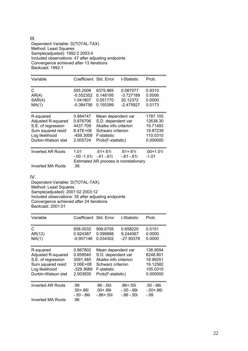
III. Dependent Variable: D(TOTAL-TAX) Method: Least Squares Sample(adjusted): 1992:2 2003:4 Included observations: 47 after adjusting endpoints Convergence achieved after 13 iterations Backcast: 1992:1 Variable Coefficient Std. Error t-Statistic Prob. C 555.2008 6375.965 0.087077 0.9310 AR(4) -0.552352 0.148195 -3.727189 0.0006 SAR(4) 1.041807 0.051770 20.12372 0.0000 MA(1) -0.384756 0.155399 -2.475927 0.0173 R-squared 0.884747 Mean dependent var 1787.105 Adjusted R-squared 0.876706 S.D. dependent var 12638.30 S.E. of regression 4437.709 Akaike info criterion 19.71493 Sum squared resid 8.47E+08 Schwarz criterion 19.87239 Log likelihood -459.3008 F-statistic 110.0310 Durbin-Watson stat 2.005724 Prob(F-statistic) 0.000000 Inverted AR Roots 1.01 .61+.61i .61+.61i .00+1.01i -.00 -1.01i -.61 -.61i -.61 -.61i -1.01 Estimated AR process is nonstationary Inverted MA Roots .38 IV. Dependent Variable: D(TOTAL-TAX) Method: Least Squares Sample(adjusted): 2001:02 2003:12 Included observations: 35 after adjusting endpoints Convergence achieved after 24 iterations Backcast: 2001:01 Variable Coefficient Std. Error t-Statistic Prob. C 658.0032 999.6705 0.658220 0.5151 AR(12) 0.924387 0.099998 9.244067 0.0000 MA(1) -0.957146 0.034302 -27.90378 0.0000 R-squared 0.867802 Mean dependent var 138.9594 Adjusted R-squared 0.859540 S.D. dependent var 8248.801 S.E. of regression 3091.485 Akaike info criterion 18.99251 Sum squared resid 3.06E+08 Schwarz criterion 19.12582 Log likelihood -329.3689 F-statistic 105.0310 Durbin-Watson stat 2.003835 Prob(F-statistic) 0.000000 Inverted AR Roots .99 .86 -.50i .86+.50i .50 -.86i .50+.86i .00+.99i -.00 -.99i -.50+.86i -.50 -.86i -.86+.50i -.86 -.50i -.99 Inverted MA Roots .96

22

Appendix B Numerous effective rates were computed, however, the 3 most applicable (closest correlation with nominal tariffs) are: Corr. coef.

EF1: total import duties/non-oil imports 0.990 EF2: non-oil import duties/non-oil imports 0.970 EF3: total collections/non-oil imports 0.995

Of which the last, EF3, is the most correlated with average nominal tariffs. This result is important to projecting the effective rate since the trend in nominal tariffs may be anticipated. Nominal tariffs were averaged from the nominal tariffs by major product chapter. Updating the averages will require a line-by-line application of “new” tariff rates, before a simple average is applied.

Actual data 1998 1999 2000 2001 2002 2003 2004 Nominal tariff 12.35 10.81 8.78 8.56 6.53 6.72 6.94 EF3 6.33 7.30 6.85 6.39 5.26 5.23 5.42

Buoyancy 1999 2000 2001 2002 2003 2004 Ave 1 Ave 2 EF1 0.81 3.07 0.37 1.35 5.37 0.93 2.36 1.08

Buoyancy was averaged by, a simple average from 2001 to 2003 (Ave 1) and averaging the years where the growth rates are similar, this is tantamount to assuming a buoyancy of 1 (Ave 2). The results are projected effective rates of 5.64 using Ave 1, and 5.42 using Ave 2. Applying the effective rates to the year-ahead import forecast of the BSP (P 2.211 trillion versus an actual of P 2.258 trillion) results in a forecast range of

BoC collection forecast: P 119.845B – P 124.719B

23