FORECASTING OUTPUT AND INFLATION: THE ROLE OF ASSET PRICES

May 2000 (This revision: February 2001)

James H. Stock Kennedy School of Government, Harvard University

and the National Bureau of Economic Research

and

Mark W. Watson* Woodrow Wilson School and Department of Economics, Princeton University

and the National Bureau of Economic Research

* We thank Charles Goodhart and Boris Hofmann for sharing their housing price data, John Campbell for sharing his dividend yield data. Helpful comments were provided by John Campbell, Fabio Canova, Steve Cecchetti, Stefan Gerlach, Charles Goodhart, Mike McCracken, Marianne Nessen and participants at the June 2000 Sveriges Riksbank Conference on Asset Markets and Monetary Policy. We thank Jean-Philippe Laforte for research assistance. This research was funded in part by NSF grant SBR-9730489.

ABSTRACT

This paper examines old and new evidence on the predictive performance of asset

prices for inflation and real output growth. We first review the large literature on this

topic, focusing on the past dozen years. We then undertake an empirical analysis of

quarterly data on up to 38 candidate indicators (mainly asset prices) for seven OECD

countries for a span of up to 41 years (1959 – 1999). The conclusions from the literature

review and the empirical analysis are the same. Some asset prices predict either inflation

or output growth in some countries in some periods. Which series predicts what, when

and where is, however, itself difficult to predict: good forecasting performance by an

indicator in one period seems to be unrelated to whether it is a useful predictor in a later

period. Intriguingly, forecasts produced by combining these unstable individual forecasts

appear to improve reliably upon univariate benchmarks.

Keywords: Large model forecasting, combination forecasts, macroeconomic forecasting

JEL Numbers: C32, E37, E47

1

1. Introduction

Because asset prices are forward-looking economic variables, they constitute a

class of potentially useful predictors of future inflation and output growth. Indeed,

Mitchell and Burns (1938) included the Dow Jones composite index in their initial list of

leading indicators of expansions and contractions in the U.S. economy. The past dozen

years has seen considerable research on the role of asset prices as predictors of future

economic activity and inflation. This interest in asset prices as leading indicators arose,

at least in part, from the instability in the 1970s and early 1980s of forecasts of output and

inflation based on monetary aggregates and of forecasts of inflation based on the (non-

expectational) Phillips curve. A large body of research on this topic now exists, and it

has identified a number of asset prices as leading indicators of either the real economy or

inflation; these include interest rates, term spreads, stock returns, dividend yields, and

exchange rates.

This paper starts by reviewing this large literature on asset prices as predictors of

real economic activity and inflation. Our review, contained in Section 2, considers 66

papers, primarily from the past twelve years. We then undertake our own empirical

assessment of the practical value of asset prices for short- to medium-term economic

forecasting. We use quarterly data on as many as 38 indicators from each of seven

developed economies (Canada, France, Germany, Italy, Japan, the U.K., and the U.S.)

over 1959 – 1999 (some series are available only for a shorter period). Most of these 38

indicators are asset prices, but for comparison purposes we also consider monetary

aggregates, selected measures of real economic activity, and some commodity prices.

2

Our analysis of the literature and the data leads to four main conclusions. First,

some asset prices have statistically significant marginal predictive content for output

growth at some times in some countries. Whether this predictive content can be reliably

exploited is less clear, for this requires knowing a-priori what asset price works when in

which countries. The argument that asset prices are useful for forecasting inflation is

weaker than for output growth.

Second, forecasts based on individual indicators are unstable. For example, in the

U.S., recursive (i.e. simulated out of sample) forecasts of the four-quarter growth of

industrial production using the term spread were substantially more accurate than a

simple autoregressive benchmark from 1971 to 1984, but were substantially less accurate

than the autoregressive benchmark from 1985 to 1999. More generally, finding an

indicator that predicts well in one period is no guarantee that it will predict well in later

periods; indeed, whether an indicator-based forecast outperforms an autoregressive

benchmark in a subsequent period appears to be independent of whether it has done so in

the past. This, along with evidence based on formal stability tests, suggests that

instability of predictive relations based on asset prices (and most other candidate leading

indicators) is the norm.

Third, although the most common method of identifying a potentially useful

predictor is to rely on in-sample significance tests such as Granger causality tests, this

turns out to provide no assurance that the identified predictive relation is stable. Indeed,

the empirical results indicate that a significant Granger causality statistic contains little or

no information about whether the indicator has been a reliable predictor.

3

Fourth, suitably combining the information in the various predictors appears to

circumvent the worst of these instability problems. For example, the median of the

forecasts of output growth based on individual asset prices produces a forecast that is

reliably more accurate than the AR benchmark, even though the individual forecasts used

to compute the median are not. Similarly, forecasts of inflation that combine information

from measures of real activity and output gaps appear to be reliable and stable, even

though the individual component forecasts are not.

2. Literature Survey

There is a vast literature on the prediction of output growth and inflation using

asset prices and other economic indicators. This survey first reviews the use of financial

indicators as predictors, then briefly summarizes recent developments in predicting

output growth and inflation using nonfinancial indicators. This review focuses on

developments in the past decade, with some historical antecedents, and encompasses 66

papers. This is followed by an attempt to draw some general conclusions from this

literature.

The main method used in this literature to establishing predictive content is to

consider significance tests (such as Granger Causality tests) or marginal R2’s in

regressions. The regressions are usually bivariate (e.g. output growth over the next four

quarters is regressed against a spread, with or without lagged output growth) but are

sometimes multivariate (in which additional predictors, such as money growth, are also

included). When these regressions are run over the full sample, the resulting statistics

will be referred to as “in sample.” Less commonly, authors construct sequences of

4

forecasts by estimating models recursively (or using a rolling sample) and, at each date,

computing an out of sample forecast; the performance of these forecasts is then compared

across models. The resulting statistics will be referred to as “simulated out of sample”

statistics.

2.1 Forecasts Using Asset Prices

Interest rates. Short term interest rates have a long history of use as predictors of

output and inflation. Notably, using data for the U.S., Sims (1980) found that including

the commercial paper rate in vector autoregressions (VARs) with output, inflation, and

money eliminated the marginal predictive content of money for real output. This result

has been confirmed in numerous studies, e.g. Bernanke and Blinder (1992) for the U.S.,

who suggested that the Federal Funds rate is the appropriate short-run measure of

monetary policy rather than the growth of monetary aggregates. Most of the research

involving interest rate spreads has, however, found that the level (or change) of a short

rate has little marginal predictive content once spreads are included.

Term spreads. The term spread is the difference between interest rates on long

and short maturity debt, usually government debt. The literature on term spreads uses

different measures of this spread, the most common being a long government bond rate

minus a 3-month government bill rate, although the long bond rate less an overnight rate

(e.g. the Federal Funds rate in the U.S.) is sometimes used.

The adage that an inverted yield curve signals a recession was formalized

empirically, apparently independently, by a number of researchers in the late 1980s,

including Laurent (1988, 1989), Harvey (1988, 1989), Stock and Watson (1989), Chen

5

(1991), and Estrella and Hardouvelis (1991). These studies primarily focused on bivariate

relations in which a measure of the term spread was used to predict output growth (or in

the case of Harvey (1988), consumption growth) using U.S. data. Of these studies,

Estrella and Hardouvelis (1991) provided the most comprehensive documentation of the

strong (in-sample) predictive content of the spread for output, including its ability to

predict a binary recession indicator in probit regressions. Most of this work focused on

bivariate relations, with the exception of Stock and Watson (1989) which used in-sample

statistics for bivariate and multivariate regressions to identify the term spread and a

default spread (the paper-bill spread) as two historically potent leading indicators for

output. The work of Fama (1990) and Mishkin (1990a, 1990b) is also notable, for they

found that the term spread has (in-sample, bivariate) predictive content for real rates,

especially at shorter horizons.

Subsequent work has focused on whether this finding is stable across time within

the U.S. and whether it holds up in international evidence. A closer examination of the

U.S. evidence has led to the conclusion that the predictive content of the term spread for

economic activity has diminished since 1985, a point made using both simulated out of

sample and rolling in-sample statistics by Haubrich and Dombrosky (1996) and Dotsey

(1998). These conclusions were based on linear models. Models that instead focus on

predicting binary recession events generally suggest that the term spread had some value

in explaining the 1990 recession. The ex post analyses of Estrella and Mishkin (1998a),

Lahiri and Wang (1996) and Dueker (1997) respectively provided probit and Markov

switching models that produce in-sample recession probabilities consistent with the term

spread providing advance warning the 1990 U.S. recession; these estimated probabilities,

6

however, were based on estimated parameters that include this recession so these are not

real time or simulated out of sample recession probabilities.

The real-time evidence about the value of the spread as an indicator in the 1990

recession is more mixed. Laurent (1989), using the term spread, predicted an imminent

recession in the U.S.; Harvey (1989) published a forecast based on the yield curve that

suggested “a slowing of economic growth, but not zero or negative growth” from the

third quarter of 1989 through the third quarter of 1990; and the Stock – Watson (1989)

experimental recession index increased sharply when the yield curve flattened in late

1988 and early 1989. However, the business cycle peak of July 1990 considerably

postdates the predicted period of these slowdowns: as Laurent (1989) wrote, “recent

spread data suggest that the slowdown is likely to extend through the rest of 1989 and be

quite significant.” Moreover, Laurent’s (1989) forecast was based in part on a judgmental

interpretation that the then-current inversion of the yield curve had special (nonlinear)

significance, signaling a downturn more severe than would be suggested by a linear

models. Indeed, even the largest predicted recession probabilities based on the in-sample

models are modest: 25% in Estrella and Mishkin’s (1998a) probit model and 20% in

Dueker’s (1997) Markov switching model, for example. One interpretation of this

episode is that the term spread is an indicator of monetary policy; that monetary policy

was tight during late 1988; and that yield-curve based models correctly predicted a

slowdown in 1989. This slowdown was not, however, a recession, and under this

interpretation the recession of 1990 was not due to monetary conditions but rather to

special non-monetary circumstances such as the invasion of Kuwait by Iraq and the

subsequent response by U.S. consumers. This interpretation is broadly similar to

7

Friedman and Kuttner’s (1998) explanation of the failure of the paper – bill spread to

predict the 1990 recession (discussed below).

Evidence on the predictive content of the term spread for real output growth in

major developed economies other than the U.S. has been examined by Plosser and

Rouwenhorst (1994), Bonser-Neal and Morley (1997), Kozicki (1997), Estrella and

Mishkin (1998b), and Campbell (1999). Bernard and Gerlach (1998) provided cross-

country evidence on term spreads as predictors of a binary recession indicator. These

studies typically used in-sample statistics and data sets that start in 1970 or later, and

there was little close examination of stability over time of predictive relations within a

country. All these studies concluded that the term spread has significant predictive

content for output growth (or, in Bernard and Gerlach’s (1998) case, for recessions) in

many developed countries, especially at horizons of one or two years. Unlike most of

these papers, Plosser and Rouwenhorst (1994) considered multiple regressions that

include the level and change of interest rates and concluded that, given the spread, the

short rate has little predictive content for output in almost all the economies they

consider.

Many studies, including some of those already cited, also considered the

predictive content of the term spread for inflation. According to the risk neutral

expectations hypothesis of the term structure of interest rates, the forward rate (and the

term spread) should embody market expectations of future inflation and the future real

rate. With some notable exceptions, the papers in this literature generally find that there is

little or no marginal information content in the nominal interest rate term structure for

future inflation. Much of the early work did not control for lagged inflation. In U.S.

8

data, Mishkin (1990a) found no predictive content of term spreads for inflation at the

short end of the yield curve, although Mishkin (1990b) found predictive content using

spreads that involve long bond rates. Jorion and Mishkin (1991) and Mishkin (1991)

reached similar conclusions using data on ten OECD countries, results confirmed by

Gerlach (1997) for Germany using Mishkin’s methodology. Drawing on Frankel’s

(1982) early work in this area, Frankel and Lown (1994) suggested a modification of the

term spread based on a weighted average of different maturities that outperformed the

simple term spread in Mishkin-style regressions. Mishkin’s regressions have a single

stochastic regressor, the term spread (no lags), and in particular do not include lagged

inflation. Inflation is, however, highly persistent, and Bernanke and Mishkin (1992),

Estrella and Mishkin (1998b), and Kozicki (1997) examined the in-sample marginal

predictive content of the term spread, given lagged inflation. Bernanke and Mishkin

(1992) found little or no marginal predictive content of the term spread for one month

ahead inflation in a data set with six large economies, once lags of inflation are included.

Kozicki (1997) and Estrella and Mishkin (1998b) included only a single lag of inflation,

but even so they found that marginal predictive content of the term spread for future

inflation is slim. For example, once lagged inflation is added, Kozicki (1997) found that

the spread remained significant for one-year inflation in only two of the ten OECD

countries she studies.

Default spreads. Another strand of research has focused on the predictive

content of default spreads, primarily for real economic activity. A default spread is the

difference between the interest rates on matched maturity private debt with different

degrees of default risk. Different authors measure this differently, and these differences

9

are potentially important. Because the market for private debt differs substantially across

countries and is most developed for the U.S., most of this work has focused on the U.S.

In his study of the credit channel during the Great Depression, Bernanke (1983)

showed that, during the interwar period the Baa – Treasury bond spread was a useful

predictor of industrial production growth. Stock and Watson (1989) and Friedman and

Kuttner (1992) studied default spread as a predictor of real growth in the postwar period;

they found that the spread between commercial paper and U.S. Treasury bills of the same

maturity (3 or 6 months; the “paper – bill” spread) was a potent predictor of output

growth (monthly data, 1959 – 1988 for Stock and Watson (1989), quarterly data, 1960 –

1990 for Friedman and Kuttner (1992)). Using in-sample statistics, Friedman and

Kuttner (1992) concluded that, upon controlling for the paper – bill spread, monetary

aggregates and interest rates have little predictive content for real output. This finding

was confirmed by Bernanke and Blinder (1992) and Feldstein and Stock (1994).

Subsequent literature focused on whether this predictive relationship is stable over

time. Bernanke (1990) used in-sample statistics to confirm the strong performance of

paper-bill spread as predictor of output, but by splitting up the sample he also suggested

that this strength weakened during the 1980s. This view was affirmed and asserted more

strongly by Thoma and Gray (1994), Hafer and Kutan (1992), and Emery (1996). Thoma

and Gray (1994), for example, found that the paper-bill spread has strong in-sample

explanatory power in recursive or rolling regressions, but little predictive power in

simulated out of sample forecasting exercises over the 1980s. Emery (1996) finds little

in-sample explanatory power of the paper-bill spread in samples that postdate 1980.

These authors interpreted this as a consequence of special events, especially in 1973 –

10

1974, which contribute to a good in sample fit but not necessarily good forecasting

performance. Drawing on institutional considerations, Duca (1999) also took this view;

indeed, Duca’s (1999) concerns echo Cook’s (1981) warnings about how the changing

institutional environment and financial innovations could substantially change markets

for short term debt and thereby alter the relationship between default spreads and real

activity.

The single most obvious true out-of-sample predictive failure of the paper-bill

spread is its failure to rise sharply in advance of the 1990 – 1991 U.S. recession. In their

post-mortem, Friedman and Kuttner (1998) suggested that this predictive failure arose

because the 1990 – 1991 recession was caused in large part by nonmonetary events that

would not have been detected by the paper-bill spread. They further argued that there

were changes in the commercial paper market unrelated to the recession that also led to

this predictive failure.

We are aware of little work examining the predictive content of default spreads in

economies other than the U.S. Bernanke and Mishkin (1992) report a preliminary

investigation, but they questioned the adequacy of their private debt interest rate data (the

counterpart of the commercial paper rate in the U.S.) for several countries. Finding long

enough time series data on reliable market prices of suitable private debt instruments has

been a barrier to international comparisons on the role of the default spread.

Some studies examined the predictive content of the default spread for inflation.

Friedman and Kuttner (1992) found little predictive content of the paper – bill spread for

inflation using Granger causality tests. Consistent with this, Feldstein and Stock (1994)

11

found that although the paper – bill spread was a significant (in-sample) predictor of real

GDP, it did not significantly enter equations predicting nominal GDP.

Four non-exclusive arguments have been put forth on why the paper – bill spread

had predictive content for output growth during the 1960s and 1970s. Stock and Watson

(1989) suggested the predictive content arises from expectations of default risk, which

are in turn based on private expectations of the economy. Bernanke (1990) and Bernanke

and Blinder (1992) argued instead that the paper-bill spread is a sensitive measure of

monetary policy, and this is the main source of its predictive content. Friedman and

Kuttner (1993a, 1993b) suggested that the spread is detecting influences of supply and

demand (i.e. liquidity) in the market for private debt; this emphasis is similar to Cook’s

(1981) attribution of movements in such spreads to supply and demand considerations.

Finally, Thoma and Gray (1994) and Emery (1996) have suggested the predictive content

is the consequence of one-off events.

There has been some examination of other spreads in this literature. Gertler and

Lown (2000) take the view that, because of the credit channel theory of monetary policy

transmission, the premise of using a default spread to predict future output is sound, but

that the paper-bill spread is a flawed choice for institutional reasons. Instead, they

suggest using the high-yield bond (“junk bond”) – Aaa spread instead. The junk bond

market was only developed in the 1980s in the U.S., so this spread has a short time series.

Still, Gertler and Lown (2000) present in-sample evidence that its explanatory power was

strong throughout this period. This is notable because the paper-bill spread (and, as was

noted above, the term spread) have substantially reduced or no predictive content for

output growth in the U.S. during this period. However, Duca’s (1999) concerns about

12

default spreads in general extend to the junk bond-Aaa spread as well: he suggests the

spike in the junk bond spread in the late 1980s and early 1990s (which is key to this

spread’s signal of the 1990 recession) was a coincidental consequence of the aftermath of

the thrift crisis, in which thrifts were forced to sell their junk bond holdings in an illiquid

market.

Stock prices and dividend yields. A simple model of stock price valuation is that

prices equal the discounted expected value of future earnings; thus stock prices or returns

should be useful in forecasting earnings or, more broadly, output growth. The empirical

link between stock prices and economic activity has been noted at least since Mitchell

and Burns (1938). Upon closer inspection, however, this link is murky. Stock returns

generally do not have substantial in-sample predictive content for future output, even in

bivariate regressions with no lagged dependent variables (e.g. Fama [1981], Harvey

[1989]), and any predictive content is reduced by including lagged output growth. This

minimal marginal predictive content is found both in linear regressions predicting output

growth (e.g. Stock and Watson [1989, 1999a]) and in probit regressions of binary

recession events (Estrella and Mishkin [1998a]).

In his review article, Campbell (1999) shows that in a simple loglinear

representative agent model, the log price-dividend ratio embodies rational discounted

forecasts of dividend growth rates and stock returns, making it an appropriate state

variable to use for forecasting. In his international dataset (fifteen countries, sample

periods mainly 1970s – 1990), Campbell (1999) found however that the log dividend

price ratio has little predictive content for output. This is consistent with the generally

negative conclusions in the larger literature that examines the predictive content of stock

13

returns directly. These generally negative findings provide a precise reprise of the

witicism that the stock market has predicted nine of the last four recessions.

Few studies have examined the predictive content of stock prices for inflation.

One is Goodhart and Hofmann (2000), who find that stock returns do not have marginal

predictive content for inflation in their international data set (seventeen developed

economies, quarterly data, mainly 1970-1998 or shorter).

Other financial indicators. Exchange rates are a channel through which inflation

can be imported in open economies. In the U.S., exchange rates (or a measure of the

terms of trade) have long entered conventional Phillips curves. Gordon (1982, 1998)

finds these exchange rates statistically significant based on in-sample tests. In their

international dataset, however, Goodhart and Hofmann (2000) find that recursive out of

sample forecasts of inflation using exchange rates and lagged inflation outperformed

autoregressive forecasts in only one or two of their seventeen countries, depending on the

horizon. At least in the U.S. data, there is also little evidence that exchange rates predict

output growth, cf. Stock and Watson (1999a).

One problem with the nominal term structure as a predictor of inflation is that,

under the expectations hypothesis, the forward rate embodies forecasts of both inflation

and future real rates. In principal, one can eliminate the expected future real rates by

using spreads between forward rates in the term structures of nominal and real debt of

matched maturity and matched bearer risk. One of the very few cases for which this is

possible with time series of a reasonable length is for British index-linked bonds. Barr

and Campbell (1997) investigated the (bivariate, in sample) predictive content of these

implicit inflation expectations and found that they had better predictive content for

14

inflation than forward rates obtained solely from the nominal term structure. They

provided no evidence on Granger causality or marginal predictive content of these

implicit inflation expectations in multivariate regressions.

Lettau and Ludvigson (1999) proposed a novel indicator, the log of the

consumption-wealth ratio. They argue that in a representative consumer model with no

stickiness in consumption, the log ratio of consumption to total wealth (human and

nonhuman) should predict the return on the market portfolio. They find that their

empirical version of the consumption – wealth ratio (a cointegrating residual between

consumption of nondurables, financial wealth, and labor income, all in logarithms) has

predictive content for multiyear stock returns. If consumption is sticky, it could also have

predictive content for consumption growth. However, Ludvigson and Steindel (1999)

found that this indicator does not predict consumption growth or income growth in the

U.S. one quarter ahead.

Housing constitutes a large component of aggregate wealth and gets significant

weight in the CPI in many countries. More generally, housing is a volatile and cyclically

sensitive sector, and measures of real activity in the housing sector are known to be

useful leading indicators of economic activity, at least in the U.S. (Stock and Watson

[1989, 1999a]), suggesting a broader channel by which housing prices might forecast real

activity, inflation, or both. In the U.S., housing starts (a real quantity measure) have

some predictive content for inflation (Stock [1998], Stock and Watson [1999b]). Studies

of the predictive content of housing prices confront difficult data problems, however.

Goodhart and Hofmann (1999) constructed a housing price data set for twelve OECD

countries (extended to seventeen countries in Goodhart and Hofmann (2000). They

15

found that residential housing inflation has significant in-sample marginal predictive

content for overall inflation in a few of the several countries they study, although in

several countries they used interpolated annual series which makes forecasting difficult to

assess.

2.2. Forecasts Using Nonfinancial Variables

The literature on forecasting output and inflation with nonfinancial variables is

massive. This section highlights a few relevant very recent studies on this topic. Many

variables have some predictive content for output growth (based on in-sample statistics),

and there is no single nonfinancial indicator that has been suggested to provide key

forecasting information for output growth. See Stock and Watson (1999a) for an

extensive review of the U.S. evidence.

The use of nonfinancial variables to forecast inflation has, to a large extent,

focused on identifying suitable measures of output gaps, that is, estimating generalized

Phillips curves. In the U.S., the unemployment-based Phillips curve with a constant

NAIRU has recently been unstable, predicting accelerating inflation during a time that

inflation has, in fact, been low or falling. This has been widely documented, see for

example Gordon (1997, 1998) and Staiger, Stock and Watson (1997a, 1997b, 2001). One

interpretation of this has been to suggest that the NAIRU has been falling in the U.S.

Mechanically, this keeps the unemployment-based Phillips curve on track, and it makes

sense in the context of changes in the U.S. labor market and in the economy generally, cf.

Katz and Krueger (1999). However, an imprecisely estimated time-varying NAIRU

makes forecasting using the unemployment-based Phillips curve problematic.

16

A different reaction to this time variation in the NAIRU has been to see if there

are alternative predictive relations that have been more stable. Staiger, Stock and Watson

(1997a) consider 71 candidate leading indicators of inflation, both financial and

nonfinancial (quarterly, U.S.), and in a similar but much more thorough exercise Stock

and Watson (1999b) consider 167 candidate leading indicators (monthly, U.S.). They

found a few indicators that have been stable predictors of inflation, the leading example

being the capacity utilization rate. Gordon (1998) and Stock (1998) confirmed the

accuracy of recent U.S. inflation forecasts based on the capacity utilization rate. Stock

and Watson (1999b) also suggested an alternative Phillips curve type forecast, based on a

single aggregate activity index computed using 85 individual measures of real aggregate

activity. These optimistic results, however, are tempered by recognizing that simulated

out of sample analysis is different than true out of sample analysis and, as Atkeson and

Ohanian (2000) show, real time published U.S. inflation forecasts have on average not

performed as well as a random walk benchmark over the past fifteen years.

The international evidence on the suitability of output gaps and the Phillips Curve

for forecasting inflation is mixed. Simple unemployment-based models with a constant

NAIRU fail in Europe, which is one way to state the so-called phenomenon of hysteresis

in the unemployment rate. More sophisticated and flexible statistical tools for estimating

the NAIRU can improve in-sample fits for the European data (e.g. Laubach [2001]), but

their value for forecasting is questionable because of imprecision in the estimated

NAIRU at the end of the sample. Similarly, inflation forecasts based on output gaps

rather than unemployment rates faces the practical problem of estimating the gap at the

end of the sample, which necessarily introduces a one-sided estimate and associated

17

imprecision. Preliminary evidence in Marcellino, Stock and Watson (2000) suggested

that the ability of output gap models to forecast inflation in Europe is more limited than

in the U.S.

Finally, there is some evidence (from U.S. data) that the inflation process itself, as

well as predictive relations based on it, is time varying. Brainard and Perry (1999)

suggested that the largest autoregressive root in inflation in the U.S. increased to a peak

in the 1970s and has declined subsequently. Akerlof, Dickens and Perry (2000) provided

a model, based on near-rational behavior, which motivates a nonlinear Phillips curve

which they interpreted as consistent with the Brainard and Perry (1999) evidence.

In a similar vein, Cecchetti, Chu and Steindel (2000) performed a simulated out of

sample forecasting experiment on various candidate leading indicators of inflation, from

1985 to 1998 in the U.S., including interest rates, term and default spreads, and several

nonfinancial indicators. They concluded that none of these indicators, financial or

nonfinancial, reliably predicts inflation in bivariate forecasting models, and that there are

very few years in which financial variables outperform a simple autoregression. Because

they assessed performance on a year by year basis, these findings have great sampling

variability and it is difficult to know how much of this is due to true instability. Their

findings are, however, consistent with Stock and Watson’s (1996) results based on formal

stability tests that time variation in these reduced form bivariate predictive relations is

widespread in the U.S. data.

18

2.3. Discussion

An econometrician might quibble with some aspects of this literature. Many of

the papers focus on bivariate relations, not even including lagged endogenous variables,

and thereby fail to asses marginal predictive content. Results often change when

marginal predictive content is considered (the predictive content of the term spread for

inflation is one example). Many of the regressions involve overlapping returns, and

when the overlap period is large relative to the sample size the distribution of in-sample t-

statistics and R2s becomes nonstandard. In many cases, such as the dividend yield or the

term spread, the regressors are highly persistent, and even if they do not have a unit root

this persistence causes conventional inference methods to break down. These latter two

problems combined make it even more difficult to do reliable inference, and few if any of

these papers tackle these difficulties with their in-sample regressions. Instability is a

major focus of some of these papers, but despite this formal tests for stability are rarely

performed. Finally, although some of the papers pay close attention to simulated

forecasting performance, in many cases predictive content is assessed primarily through

in-sample fits that require constant parameters (stationarity) for external validity.

Despite these reservations, the literature does suggest four general conclusions.

First, the variables with the clearest theoretical justification for use as predictors often

have scant empirical predictive content. The expectations hypothesis of the term

structure of interest rates suggests that the term spread should forecast inflation, but it

generally does not once lagged inflation is included. Stock prices and log dividend yields

should reflect expectations of future real earnings, but empirically they provide poor

forecasts of real economic activity. Default spreads have the potential to provide useful

19

forecasts of real activity, and at times they have, but the obvious default risk channel

appears not to be the relevant channel by which these spreads have their predictive

content. Moreover, the particulars of forecasting with these spreads seem to hinge on the

current institutional environment.

Second, there is evidence that the term spread is a serious candidate as a predictor

of output growth and recessions. The stability of this proposition in the U.S. is

questionable, however, and its universality is unresolved.

Third, although only a limited amount of international evidence on the

performance of generalized Phillips curve models was reviewed above, generalized

Phillips curves and output gaps appear to be one of the few ways to forecast inflation that

have been reliable. These particulars, too, seem to depend on the time and country.

Fourth, our reading of this literature suggests that many of these forecasting

relations are ephemeral. To a considerable degree, the work on using asset prices as

forecasting tools over the past decade was a response to disappointment over the

perceived inability of monetary aggregates to serve as reliable and stable forecasting tools

and as useful indicators of monetary policy. The evidence of the 1990s on the term

spread, the paper-bill spread, and on some of the other theoretically suggested financial

indicators recalls the difficulties that arose when monetary aggregates were used to

predict the turbulence of the late 1970s and 1980s. In this longer view, then, this

literature reflects a continuation of the ongoing breakdown of predictive relations once

seen as reliable and theoretically motivated.

20

3. Forecasting Models and Statistics

3.1. Forecasting Models

We consider models for forecasting real output growth and price inflation using a

sample of quarterly observations. Real output is measured by real GDP (RGDP) and by

the index of industrial production (IP). Prices are measured by the consumer price index

(CPI) and by the implicit GDP deflator (PGDP). The forecasting models use a candidate

predictor, tX , to predict the value of the variable of interest h quarters ahead, ht hy + , given

values of some other predictor time series tZ . The models are of the form,

( ) ( ) ( )h ht h t t t t hy L y L X L Zµ α β γ ε+ += + + + + , (3.1)

where ( )Lα , ( )Lβ and ( )Lγ are lag polynomials. All the forecasting models include lags

of the dependent variable, ty . The models differ regarding whether additional predictors,

tZ , are included, in addition to the candidate leading indicator.

The "h-step ahead projection" approach reflected in (3.1) contrasts with the more

common approach of estimating a one-step ahead model, and then iterating that model

forward to obtain h-step ahead predictions. There are two main advantages of the h-step

ahead projection approach. First, it eliminates the need for estimating additional

equations for simultaneously forecasting tX and tZ , e.g. by a VAR. Second, it reduces

the potential impact of specification error in the one-step ahead model (including the

equations for tX and tZ ) by using the same horizon for estimation as for forecasting.

Implementation of (3.1) requires making a decision about how to model the order

of integration of the dependent variable. For each country the logarithm of output is

treated as I(1), so that ty is the growth rate of output. There is, however, some ambiguity

21

about whether the logarithm of prices is best modeled as being I(1) or I(2), and so the

analysis was carried out using both transformations. The out-of-sample forecasts proved

to be more accurate for the I(2) transformation, and to save space, we present only these

results here. Thus for the price series, ty is the first difference of inflation.

The multistep forecasts are designed to examine the predictability of the

logarithm of the level of the variable, after imposing the I(1) or I(2) constraint. Letting Yt

denote the logarithm of level of the series, then ht h t h ty Y Y+ += − for real output, and

1 1(1 ) ( ) ( )ht h t h t t t h t t ty Y h Y hY Y Y h Y Y+ + − + −= − + + = − − − for prices.

Lag lengths and estimation. Two approaches are used for setting the lag lengths in

the empirical models. Because each country and series would be expected to have

different dynamics, it is natural to use data-dependent lag lengths to adapt to these

differences. Our out-of-sample forecast simulations use this approach. To make in-

sample results comparable across series and country we instead use fixed lag lengths.

Autoregressive forecasts. The autoregressive forecasts are constructed from (3.1),

omitting the terms in tX and tZ . Four quarterly lags are used for ( )Lα for the fixed lag

results. For the data-dependent lag lengths, the lag polynomial ( )Lα contained between

zero and four non-zero coefficients.

Bivariate forecasts. The bivariate forecasts introduce tX into (3.1). Four

quarterly lags are used for ( )Lα and ( )Lβ for the fixed lag results. For the data-

dependent lag lengths, ( )Lα contained between zero and four non-zero coefficients and

( )Lβ contained between one and four non-zero coefficients.

22

Forecasts with a base predictor. These forecasts introduce the base predictor, tZ ,

into (3.1), as well as the candidate leading indicator tX . For the data-dependent lag

lengths, the orders of ( )Lα and ( )Lγ contained between zero and four non-zero

coefficients and ( )Lβ contained between one and four non-zero coefficients.

Combination forecasts. The combination forecasts are constructed from groups

of individual forecasts, each based on a candidate leading indicator. The theory of

optimal linear forecast combination (Bates and Granger (1969), Granger and Ramanathan

(1984)) suggests that combination forecasts should be weighted averages of the

individual forecasts, where the optimal weights correspond to the theoretical regression

coefficients in a regression of the true future value on the various forecasts. In practice,

the feasible regression estimator of these weights can produce imprecise estimates

because of the fairly short period over which the panel of forecasts is observed, because

of a relatively large number of forecasts to be combined, and/or because of the colinearity

between the individual forecasts.

Several approaches are available to address this problem. One simple approach is

to weight forecasts in inverse proportion to their historical mean squared forecast error;

simpler yet is just to use equal weights, so that the combination forecast is a simple

average. Both methods can work well in practice, but like all linear combination methods

they can be sensitive to large outliers.

For the results reported below we report the median forecast of a group and the

trimmed mean (after eliminating the largest and smallest forecasts), two schemes that are

robust to outliers. Combined forecasts are computed for forecasts based on four groups

of indicators: real activity variables, prices and wages, monetary aggregates, and asset

23

prices. The variables in each group are listed in the data appendix. In addition, an

overall combined forecast is reported. This is computed from the group combined

forecasts; it is their median when median combined is used, and it is their mean when the

group forecasts were computed as a trimmed mean.

3.2. Model Comparison Statistics

Two sets of statistics are presented for each forecasting model. The first is based

on estimation results for the full sample. The second summarizes the performance of the

various models in a simulated out of sample forecasting experiment over two out of

sample periods.

Full sample statistics. The full-sample statistics summarize the predictive content

of the candidate leading indicator and examine the stability of the forecasting relation.

These were computed from 1-step ahead regression (h=1 in (3.1)). Statistical

significance is summarized by the Granger-Causality statistic, computed as the

heteroskedasticity consistent F-test of the hypothesis that ( ) 0Lβ = in (3.1).

The full-sample stability tests are computed by permitting the coefficients in (3.1)

to take on two values, one for observations through date τ and another subsequently. The

maximum value of the HAC Wald statistic testing the equality of the coefficients is then

computed for [.15T] < τ < [.85T], where [• ] denotes the greatest lesser integer and T is

the number of observations over which the regression is run. This statistic is the Wald

version (with HAC standard errors) of the Quandt likelihood ratio (QLR) statistic

(Quandt [1960]) and is variously termed in the literature the QLR and sup-Wald statistic;

we shall call it the QLR statistic. Two versions of this test were computed. The first tests

24

for changes in all of the coefficients in (3.1). The second tests for changes in the constant

term, µ, and β(L) only. The qualitative results were the same for both statistics, and to

save space, we report results for the second test only.

Forecast comparison statistics. The forecast comparison statistics are based on a

panel of forecasts computed for each model, horizon, and series being forecasted. The

forecasts are computed on a simulated out of sample basis, that is, all estimation, model

selection, weighting, etc. used to forecast ht hy + are based solely on data available through

date t. The models are re-estimated recursively as the forecasting exercise proceeds

through time. This produces a series of forecast errors, |ˆh ht h t h ty y+ +− (which, for h>1, are

overlapping). This simulates ongoing real time estimation and forecasting. The only

deviation from true real time forecasting is our use of the most current set of historical

data, rather than the provisional data that is available in true real time.

For most series, the out-of-sample forecasting exercise begins in the first quarter

of 1971 and continues until the end of the sample period. For variables available from

1959 onward, this allowed roughly ten years of data for estimation of the model for the

first forecast. For variables with later start dates, the out of sample forecast period began

after 10 years of in-sample data had accumulated. The out of sample period is divided

into two sub-periods 1971-84 and 1985-99. These periods are of equal length for the 4

quarter ahead forecasts.

The forecast comparison statistics examine the performance of the various

forecasts, relative to a benchmark forecast. We focus on the mean squared error of the

candidate forecast computed over the simulated out of sample subperiod, relative to the

mean squared error of the benchmark forecast, computed over the same period. When the

25

models are non-nested, HAC standard errors for this relative mean squared error can be

computed following West (1996). When the models are nested, the distribution theory is

more involved although, in principal, test statistics as discussed in Clark and McCracken

(2000) can be used. In the empirical work below, however, the simulated out of sample

periods are at times rather short. Because of the current lack of knowledge of the finite

sample performance of these procedures we do not report standard errors or tests of

forecast equality.

4. Data

Data were obtained from four main sources: the International Monetary Fund’s

IFS database (IFS), the OECD database (OECD), the DRI Basic Economics Database

(DRIBASE), and the DRI International Database (DRIINTL). Series, their source, and

transformations are listed in the appendix. Monthly and quarterly data were collected for

the 1959-1999 sample period, although many series are available only for a shorter

period. Table 1 summarizes the data available for the variables for each country.

The data were subject to five possible transformations. First, many of the data

showed significant seasonal variation, and these series were seasonally adjusted.

Seasonal variation was determined by a pre-test (regressing an appropriately differenced

version of the series on a set of seasonal dummies) carried out at the 10% level. Seasonal

adjustment was carried out using a linear approximation to X11 (Wallis’s (1974) for

monthly series and Larocque’s (1977) for quarterly series) with endpoints calculated

using autoregressive forecasts and backcasts. Second, a few of the series contained large

outliers, associated with strikes, variable re-definitions etc. Values of the (appropriately

26

differenced version of the) series that were larger than five times the inter-quartial range

were replaced with an interpolated value constructed as the median of the values within

three periods of the outlier. Third, when the data were available on a monthly basis, the

data were aggregated to quarterly observations. For the index of industrial production and

the CPI (the variables being forecast) quarterly aggregates were formed as averages of

the monthly values. For all other series, the last monthly value of the quarter was used as

the quarterly value. Fourth, in some cases the data were transformed by taking

logarithms. Finally, the highly persistent or trending variables were differenced or, when

gap variables were being constructed as deviations from an estimated trend, which we

now describe.

These gap variables were constructed as the deviation of the series from a one-

sided version of the Hodrick-Prescott (1981) (HP) filter. The one-sided HP filter is

convenient and, importantly, preserves the temporal ordering of the data. The one-sided

HP trend estimate is constructed as the Kalman filter estimate of tε from the model

2

t t t

t t

y

e

τ ε

τ

= +

∆ =

where ty is the observed series, tτ is it’s unobserved trend component, and tε and te are

mutually uncorrelated white noise sequences with relative variance var( ) / var( )t tq eε= .

As discussed in Harvey and Jaeger (1993) and King and Rebelo (1993), the HP-filter is

the optimal (linear minimum mean square error) two-sided trend extraction filter for this

model. Because our focus is on forecasting, we use the optimal one-sided analogue of

this filter, so that future values of ty (which would not be available for real time

27

forecasting) are not used in the detrending operation, and set q=.00675, which

corresponds to the usual value of the HP smoothing parameter (λ=1600).

5. Results for Models with Individual Indicators

5.1 Forecasts of Inflation

The performance of the various individual indicators relative to the autoregressive

benchmark are summarized in Table 2 for four-quarter ahead forecasts of CPI inflation.

(Comparable tables for horizons h = 2 and 8 for these variables, and for horizons h = 2, 4,

8 for PGDP, are given in the Results Appendix, Table B.1). The first row in each table

provides the root MSFEs of the simulated out of sample benchmark univariate

autoregressive forecasts in the two sample periods. For the subsequent rows, each cell

corresponds to an indicator/country pair, where the two entries are for the two sample

periods.

Inspection of Table 2 reveals that some variables forecast relatively well in some

countries in one or the other subsamples. For example, forecasts of inflation based on the

employment gap have a relative MSFE of 0.7 in the second subsample in Canada,

indicating a 30% improvement over this period relative to the benchmark autoregression.

The capacity utilization rate works well for the U.S. during both subsamples. Monetary

aggregates, especially M2 and real M2, predicted well for Germany in the first period

(but no better than the AR in the second).

These forecasting “successes,” however, appear to be isolated and sporadic. For

example, monetary aggregates rarely improve upon the AR model except in the first

period for Germany. Similarly, although housing price inflation predicts CPI inflation in

28

the first period in the U.S., it performs substantially worse than the AR benchmark in the

second period in the U.S. and in the other countries. Commodity price inflation works

well in the U.S. in the first period but not in the second; in Canada, it works well in the

second period but not in the first; and in some country/period combinations it works

much worse than the AR benchmark.

The only set of predictors that usually improve upon the AR forecasts are the

measures of aggregate activity. For example, the IP and unemployment gaps both

improve upon the AR (or are little worse than the AR) for both periods for Canada,

Germany, the U.K. and the U.S. Even for these predictors, however, the improvement is

neither universal nor always stable.

5.2 Forecasts of Output Growth

Table 3 summarizes the performance of the individual indicator forecasts of IP

growth at the four quarter horizon (results for the other horizons for IP, and for all

horizons for RGDP, are given in the Results Appendix, Table B.1). Table 3 has the same

format as Table 2

Like the inflation forecasts, it is possible to find some predictors that improve

upon the AR forecast in some countries in one or the other period. Also like the inflation

forecasts, these improvements typically are neither universal nor stable. For example,

real stock returns produced IP forecasts with a relative MSFE of 0.59 in the U.S. in the

first period, but with a relative MSFE of 2.06 in the second period. Forecasts using real

M2 growth exhibit a similar pattern.

29

In some cases, entire classes of predictors fail to improve upon the AR forecast.

For example, oil prices and commodity prices typically produce forecasts much worse

than the AR forecast, and forecasts based on output gaps generally have performance

similar to, but slightly worse than, the AR forecasts.

The forecasts based on the term spread are of particular interest, given their

prominence in the literature. In the U.S., these forecasts improve upon the AR

benchmark in the first period, but in the second period they are much worse than the AR

forecasts (the relative MSFE is 0.53 in the first period but 2.59 in the second). This is

consistent with the literature reviewed in Section 2.1, which found a deterioration of the

forecasting performance of the term spread as a predictor of output growth since 1985. In

some other cases, the term spread improves substantially upon the benchmark (Germany

in the first period, France in the second), but the evidence across countries on its

usefulness is mixed.

5.3 Forecast Stability

If the forecasting relations examined in Tables 2 and 3 are stable, then a forecast

that outperforms the benchmark in the first period would (in expectation) outperform the

benchmark in the second period. In contrast, one symptom of unstable forecasting

relations would be if an indicator outperforms the benchmark in one period but not in the

other.

Summary evidence on the stability of these forecasting relations is given in Table

4. This table summarizes the fraction of times that the relative mean squared error is

better or worse than the benchmark model in one or the other periods, out of the total of

30

962 combinations of indicators, countries, and dependent variables, for each of the three

different forecast horizons. For example, as summarized in panel A, of the 962

indicator/country/dependent variable combinations, 31% performed better than the

benchmark AR in the first period for 2-quarter ahead forecasts, 33% performed better

than the benchmark AR in the second period, and 10% performed better than the

benchmark AR in both periods.

The binary variables cross-tabulated in Table 4 appear to be approximately

independently distributed. For all cells the joint probabilities are very nearly the product

of the marginal probabilities. For example, in panel A, if the row and column variables

were independent then the probability of an indicator/country/dependent variable

combination outperforming the benchmark would be .31�.33 = .10, which is the

empirically observed probability; the corresponding calculations for the 4-quarter ahead

forecast (panel B) is a predicted probability of .36�.33 = .12, with an empirical joint

probability of .12, and for the 8-quarter forecasts (panel C) the predicted probability is

.13 while the empirical joint probability is .16. Because the draws are not independent, a

conventional test for independence of the row and column variables is inappropriate.

Still, these calculations suggest that whether an indicator/country/dependent variable

combination outperforms the benchmark in one period is effectively independent of

whether it does so in the other period.

This lack of a relation between performance in the two subsamples is also evident

in Figure 1, which is a scatterplot of the logarithm of the relative MSFE in the first vs.

second periods for the 962 combinations at the 4 quarter horizon tabulated in Table 4B.

If indicators that perform well in the first period tend to perform well in the second

31

period, then there would be relatively more points in the lower left quadrant than the

upper left or lower right quadrants, but this is not the case. Indeed, there are quite a few

points in the upper left quadrant, corresponding to indicators that perform well in the first

period but poorly in the second.

It is possible that this apparent instability is limited to a few categories of

predictors or to either output or inflation forecasts. This possibility is explored in Table

5, which summarizes the information of Table 4, broken down by category of indicator

and by whether the forecast is of output or inflation. Specifically, for each predictor

category, horizon, and type of dependent variable, the entries are the fraction of times

that an indicator/country/dependent variable outperforms the benchmark in the first

period, in the second period, and jointly in the first and second period. The final two

entries in each cell are the predicted joint probability assuming the first and second period

random variables are independent, and the number of occurrences in the cell. A

comparison of the empirical joint probability and the predicted probability under

independence reveals that, for every predictor category, these the first and second period

events are approximately independently distributed, both for forecasts of inflation and of

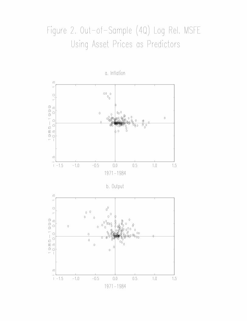
output. A scatterplot of the relative MSFEs for asset price indicators, broken down by

inflation forecasts and output forecasts, is given in Figure 2; like Figure 1, there is no

apparent pattern in these scatterplots.

Table 6 reports a similar exercise, broken down by country rather than by

category of indicator. The results are quite similar across countries, and are similar to

those in Table 5: whether an indicator/dependent variable combination is better or worse

32

than the AR in the first period is effectively distributed independently of whether it is

better or worse in the second.

In short, there appear to be no subsets of countries, predictors, or variables being

forecast that are immune to this instability. This instability is quantitatively important

from a forecasting perspective: forecasting models that outperform the AR in the first

period may, or may not, outperform the AR in the second, but whether they do appears to

be random.

5.4 Full-Sample Tests for Predictive Content and Instability

The foregoing results suggest that the instability is quantitatively large. This

section addresses two related questions. First, is this instability simply an artifact of

sampling variability, or is there formal statistical evidence of instability in these

relations? Second, even if there is this instability in some relations, it might be that this

instability results in the indicator failing to exhibit full-sample predictive content.

Accordingly, will this instability be avoided if one uses the full-sample Granger causality

statistic to identify a statistically significant forecasting relation?

Table 7 summarizes the results of performing full-sample Granger causality tests

for predictive content and QLR tests for instability in these relations. Each cell in Table

7 has five entries: the fraction of times that the Granger causality statistic for that

predictor category/dependent variable combination is significant at the 5% level; the

fraction of times that the QLR statistic is significant at the 5% level; the fraction of times

that both are significant; the product of the fraction of times they are individually

significant; and the number of cases in the cell.

33

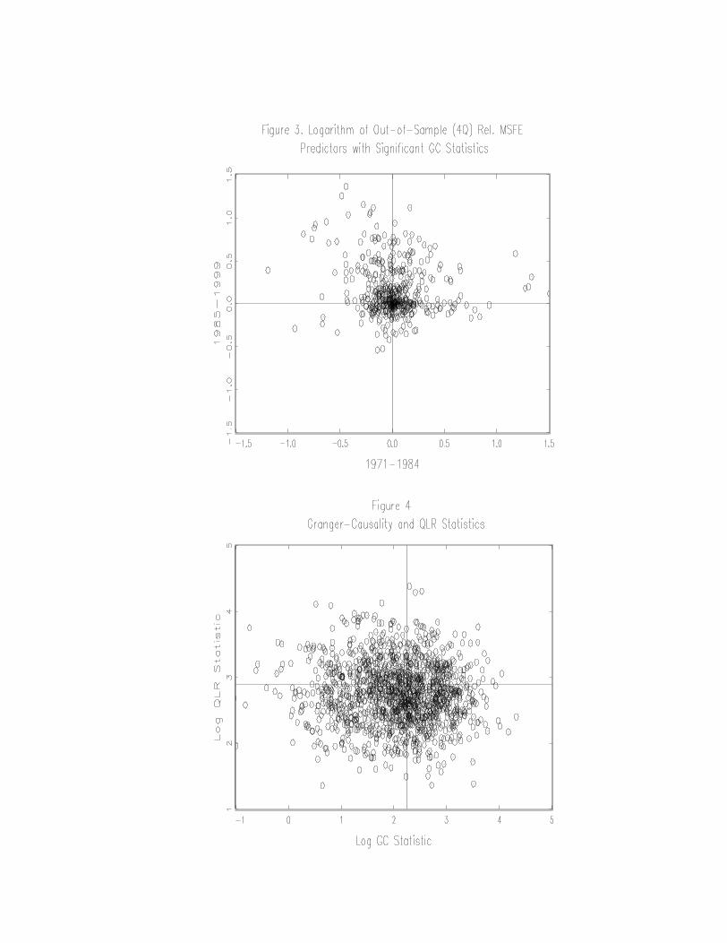
Figures 3 and 4 examine whether selecting an indicator based on a statistically

significant Granger causality statistic reduces the chances of that predictive relation being

unstable. Specifically, Figure 3 presents a scatterplot of the logarithm of the relative

MSFEs in the two subsamples, among only those predictor/country/dependent variable

combinations which have a significant full-sample Granger causality statistic. Figure 4

presents related evidence on the relation between the full sample tests for predictability

and stability, specifically, a scatterplot of the full sample QLR statistic vs. the Granger

causality statistic.

Four results are apparent from Table 7 and Figures 3 and 4. First, the full-sample

Granger causality tests are often statistically significant: 45% of the total of 1484

indicator/country/dependent variable combinations have Granger causality tests that

reject at the 5% level. This is not surprising, since these variables have in part been

chosen because there are empirical and/or theoretical reasons to believe they have

predictive content. Inspection of the results for each individual

indicator/country/dependent variable combination (given in the Results Appendix, Table

B.2) reveals that the Granger causality results are generally consistent with those in the

literature. For example, the term spread is a statistically significant predictor of output

growth (IP) at the 5% level in five of the seven countries (Japan and the U.K. being the

exceptions). Exchange rates (real or nominal) are not significant at the 5% level for any

of the countries, but short term interest rates are significant for most of the countries.

Real activity variables (the IP gap, the unemployment rate, and capacity utilization) are

significant in most of the inflation equations. The Granger causality tests suggest that

housing prices have some predictive content for real growth, at least in some countries.

34

Second, a large fraction – 37% of the total of 1484 – of the relations are unstable,

according to the QLR statistic. This suggests that the instability revealed by the analysis

of the relative MSFEs in the two subsamples is not a statistical artifact but rather is a

consequence of unstable population relations.

Third, a statistically significant Granger causality statistic conveys little if any

information about whether the forecasting relation is stable. This can be seen in several

ways. For example, the scatterplot in Figure 3 is much like the scatterplot in Figure 1:

conditioning on the full-sample Granger causality statistic does not change the joint

distribution of the relative MSFEs in the two periods. In particular, a significant Granger

causality statistic makes it no more likely that a predictor outperforms the AR in both

periods. Similarly, the scatterplot in Figure 4 suggests that the Granger causality and

QLR statistics are independently distributed. Moreover, the product of the empirical

probability that the Granger causality statistic rejects and the probability that the QLR

statistic rejects, given in Table 7, approximately equals the joint empirical probability that

both reject, consistent with these events being distributed independently.

Fourth, these findings hold, with some variation, for all the predictor

category/country/dependent variable combinations examined in Table 7. The QLR

statistics suggest a greater amount of instability in the inflation forecasts than in the

output forecasts, the greatest instability in Japan and the least in Germany. Among

predictor category/dependent variable pairs, the greatest instability is among activity

variables as predictors of inflation, and the least is among activity variables as predictors

of output. In all cases, however, the QLR and Granger causality statistics appear to be

approximately independently distributed.

35

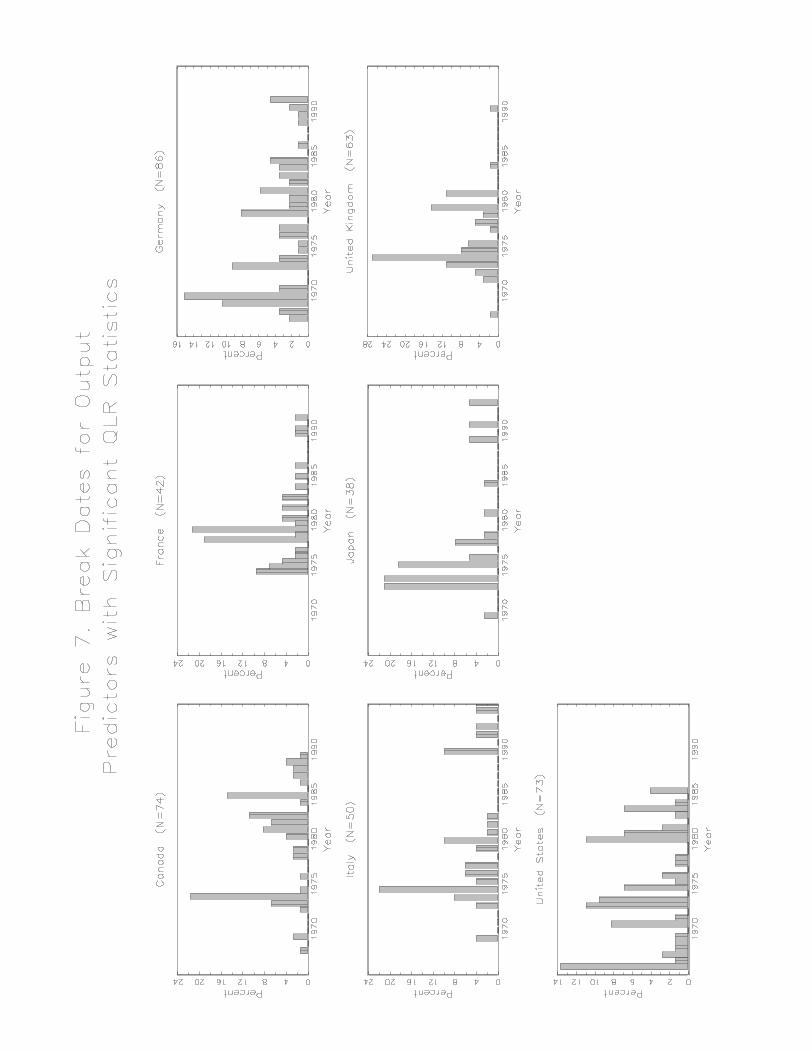
5.5 Estimated Break Dates

This evidence points to widespread instability in the empirical forecasting

relations. This raises the question of whether there are patterns in this instability. For

example, is the instability associated with discrete changes, or breaks, in the relations,

and if so, do the dates at which these breaks occur exhibit any patterns? Are these break

dates the same for output forecasts and inflation forecasts, and do these break dates differ

across countries?

This section provides an initial investigation into some of these issues. Here, we

adopt the break model, so that the instability is modeled as a distinct regime shift at an

unknown break date. If there is a single break, then it is possible to estimate the break

date consistently by least squares; if there are multiple regime breaks, then the least

squares estimator is consistent for one of the break dates (Bai [1997]).

The distribution of the estimated break dates for those indicator/country/

dependent variable combinations with a significant QLR statistic is given in Figure 5.

Both the distribution of break dates for inflation forecasts (Figure 5(a)) and for output

forecasts (Figure 5(b) have two peaks, one during 1974 – 1975 and one during 1979 –

1981, and both distributions have very few estimated breaks occurring since 1985.

These break date distributions are broken down by country in Figure 6 (inflation

forecasts) and Figure 7 (output forecasts). The results show considerable heterogeneity

in the distribution of estimated break dates across countries. At one extreme, in the U.K.

the breaks are concentrated in the 1974 – 1975 period, for both inflation and output

forecasts. In contrast, in Germany there is no apparent clustering of break dates for either

36

type of forecast. For the U.S., inflation forecasts exhibit breaks in the 1974 – 1975 and

1979 – 1981 periods, but there is less clustering of the estimated break dates for the

output forecasts.

5.6 Monte Carlo Simulation

We performed a Monte Carlo experiment to provide additional evidence on

whether the apparent instability found in the relative MSFEs might simply be a

consequence of the sampling variability of these statistics when in fact the predictive

relations are stable but heterogeneous across predictors and countries.

The design of the Monte Carlo experiment was chosen to match an empirically

plausible null model of stable but heterogeneous predictive relations. Specifically, for

each indicator/country/dependent variable pair, the full available data set was used to

estimated the VAR, 1( )t t tZ A L Z vµ −= + + , where Zt = (yt, xt), where yt is the variable to

be forecast and xt is the candidate indicator. For each pair, this produced estimates of the

VAR parameters (µ, A(L), Σv). The set of all 1484 such estimates is the joint empirical

distribution of the VAR parameters computed using this sample.

With this empirical distribution in hand, the artificial data were drawn as follows:

1. VAR parameters (µ, A(L), Σv) were drawn from the joint empirical

distribution.

2. Artificial data on Zt = (yt, xt) were generated according to a bivariate VAR

with these parameters, with the number of observations matching the full

sample used in the empirical analysis.

37

3. Benchmark forecasts of yt were made using the recursive AR forecasting

method described in Section 3.

4. Bivariate forecasts of yt were made using the recursive multistep ahead

forecasting method based on (3.1).

5. Relative MSFEs for the two periods (simulated 1971 – 1984 and 1985 – 1999)

were computed as described in Section 3.

Thus the distributions of the relative MSFEs incorporates generated in this design

incorporates both the sampling variability of these statistics, conditional on the VAR

parameters, and the (empirical) distribution of the estimated VAR parameters.

The results are summarized in Table 8. The main finding is that the distribution

of the difference in the relative MSFEs is much tighter in the Monte Carlo simulation

than in the actual data: both the empirical interquartile range and the difference between

the 10% and 90% percentiles is approximately three times the corresponding figures for

the simulated statistics. That is, sampling variation is insufficient to explain the dramatic

shifts in predictive content observed in the data, even after accounting for the

heterogeneity in the predictive relations. In other words, if the predictive relations are

stable, it is extremely unlikely that we would have observed as many cases as we actually

did with small relative MSFEs in the first period and large relative MSFEs in the second

period.

5.7 Trivariate Models

In addition to the bivariate models, we considered forecasts based on trivariate

models. The trivariate models for inflation included lags of inflation, the IP gap, and the

38

candidate indicator. The trivariate models for output growth included lags of output

growth, the term spread, and the candidate indicator. (The particulars are discussed in

Section 3).

MSFEs, relative to the benchmark AR model, are given for all

indicators/countries/dependent variables/horizons in the Results Appendix (Table B.3).

The main conclusions drawn from the bivariate models also hold for the trivariate

models. In some countries and some time periods, some indicators perform better than

the bivariate model. For example, in Canada it would have been desirable to use the

unemployment rate in addition to the IP gap for forecasting CPI inflation in the second

period (but not the first); in Germany it would have been desirable to use M2 growth in

addition to the IP gap in the first period (but not the second).

There are, however, no clear systematic patterns of improvement when candidate

indicators are added to the bivariate model. Rather, the main pattern is that the trivariate

relative MSFEs show subsample instability similar to those of the bivariate relative

MSFEs. This instability is, presumably, in part driven by the instability of bivariate

relation which the trivariate relation extends, that is, the instability of the term spread as a

predictor of output growth and the instability of the IP gap as a predictor of inflation. For

example, all the trivariate models of output growth perform poorly in the U.S. in the

second period, which reflects the poor performance of the term spread over this period.

But the trivariate results suggest that adding another indicator to this relation does not

reduce this instability, indeed often the resulting trivariate predictive models appear even

less stable than the base bivariate model.

39

6. Results for Combination Forecasts

This section examines the possibility that combining the forecasts based on the

individual indicators can improve their performance. The combination forecasts

considered here are the trimmed mean forecast from the full set of forecasts or from a

subset of the forecasts, as discussed in Section 3. The results for combination forecasts

based on the median are given in the Results Appendix. As it happens, the two methods

give very similar results.

The results are summarized in Table 9. The entries are relative MSFEs of the

combined forecast among the forecasts corresponding to each cell (that is, the trimmed

mean forecast among a group of indicators at a specified horizon for a particular

country).

The results in Table 9 are striking. First consider the results for inflation (panels

A and B of Table 9). The trimmed mean of all the individual indicator forecasts of CPI

inflation outperforms the benchmark AR in every country, in both periods, and at all

three horizons. The overall combination GDP inflation forecasts improve upon the

benchmark AR in every country in each period for the four- and eight-quarter ahead

forecasts, and in all but two countries for the two-quarter ahead forecasts, and in these

two cases (Japan and the U.S., both in the first period) the loss relative to the AR is very

small.

Inspection of the results for different groups of indicators reveals that these

improvements are realized across the board. For the Canada, Germany, the U.K. and the

U.S., the greatest improvements are obtained using the combination forecasts based

solely on the activity indicators, while for France, Italy and Japan the gains are typically

40

greatest if all the indicator forecasts are used. In many cases, the combination forecasts

have relative MSFEs under 0.80, so that these forecasts provide substantial improvements

over the AR benchmark.

The results for combination forecasts of output growth are given in panels C and

D of Table 9. The results are qualitatively similar to those for the inflation forecasts,

although the gains relative to the benchmark are somewhat smaller. Among the 39

combinations of country, dependent variable, and horizon, the combined forecast taken

over all the individual indicator forecasts improves over the AR benchmark in all but 3

cases, and in these three cases the loss relative to the AR is less than 5%. In some cases,

these improvements are large.

Even though the individual forecasts based on asset prices are unstable, the

combined asset price forecast of output growth performs well across the different

horizons and countries. Notably, in the U.S. the relative mean squared forecast error for

eight-quarter ahead forecasts of industrial production growth based on the combined asset

price forecast is 0.44 in the first period and 0.86 in the second period.

Results for combining forecasts based on the trivariate models are presented in the

Results Appendix (Table B.3). The trivariate forecasts typically improve upon the

benchmark AR forecasts, however the improvements are not as reliable, nor are they

usually as large, as for the bivariate forecasts. For example, the trimmed mean

combination of the bivariate forecasts of four-quarter ahead CPI inflation over all

indicators in the U.S. have relative MSFEs less than one in all country/period

combinations, but for the trivariate models these exceed one in three country/period

combinations. We interpret this as arising because the trivariate models all have an

41

indicator in common (the IP gap for inflation, the term spread for output). This induces

common instabilities across the trivariate models, which in turn reduces the apparent

ability of the combination forecast to “average out” the idiosyncratic instability in the

individual forecasts.

7. Discussion and Conclusions

These results provide some evidence that asset prices have small marginal

predictive content for output at the two, four, and eight quarter horizon. However, no

single asset price works well across countries over multiple decades. The term spread

perhaps comes closest to achieving this goal, but there is substantial evidence of

instability of the term spread as a predictor. As for inflation, after controlling for lagged

inflation there is little or no evidence that individual asset prices or spreads systematically

help to predict inflation at horizons through two years. A striking regularity in the

forecasts based on individual indicators, at all horizons and for all variables being

forecasted, is the instability of the forecasts. In our simulated out of sample forecast

comparison, we found that whether a variable forecasts better than an autoregression in

the first out of sample period is essentially unrelated to whether it will do so in the second

period. These results are consistent with our reading of the literature, in which an initial

series of papers identifies what appears to be a potent a predictive relation, which is

subsequently found to break down in the same country, or not to be present in other

countries, or both.

Some might respond by suggesting that this instability is no surprise, that the

predictive power of asset prices should depend on the nature of the shocks hitting the

42

economy, and that the degree of development of financial markets and other institutional

details differ across countries. Indeed, this perspective generalizes the particular

arguments made in some of the papers reviewed in section 2, such as Cook (1981) and

Duka (1999), which provide detailed institutional interpretations of the predictive power

of specific asset prices. These considerations would suggest that asset prices that forecast

well in one country or in one period might not do so in another. Perhaps so; but we

would stress that if these indicators are to be used prospectively for forecasting, then

according to this argument one must know the nature of future macroeconomic shocks

and institutional developments that would make a particular candidate indicator stand out.

It is one thing to understand ex post why a particular predictive relation broke down; it is

quite another to know whether it will ex ante.

The results are not entirely negative, however. Rather than focusing on individual

asset prices, all of which have their deficiencies as leading indicators, these results

suggest instead that combining information from a large number of asset prices can lead

to reliable forecasts. Given the small number of observations and the apparent instability

of the individual predictive regressions, conventional regression techniques are arguably

not a good way to combining this information. In the results here, we found that useful

information could be gleaned from the asset price indicators by pooling the individual

indicator forecasts, either by computing a trimmed mean or the median forecast. These

combination forecasts seem to result in reliable improvements and also appear to avoid

the worst mistakes made using individual leading indicators. However, we provide no

theory for why these forecasts should work as well as they do, and understanding these

issues remains an ongoing challenge.

43

References Atkeson, A. and L. Ohanian (2000), “Are Short-Run Inflation Forecasts Useful for

Guiding Monetary Policy?” manuscript, Federal Reserve Bank of Minneapolis. Akerlof, G.A., W.T. Dickens, and G.L. Perry (2000), “Near-Rational Wage and Price

Setting and the Optimal Rates of Inflation and Unemployment,” Brookings Papers on Economic Activity 2000 (1), forthcoming.

Bai, J. (1997), “Estimating Multiple Breaks One at a Time,” Econometric Theory 13,

315-352, 1997. Barr, D.G. and J.Y. Campbell (1997), “Inflation, Real Interest Rates, and the Bond

Market: A Study of U.K. Nominal and Index-Linked Government Bond Prices,” Journal of Monetary Economics 39, 361 – 383.

Bates, J.M and Granger, C.W.J. (1969), “The Combination of Forecasts,” Operations

Research Quarterly, 20, 319-25. Bernanke, B.S. (1983), “Nonmonetary Effects of the Financial Crisis in the Propagation

of the Great Depression,” American Economic Review 73 (3), 257 – 276. Bernanke, B.S. (1990), “On the Predictive Power of Interest Rates and Interest Rate

Spreads,” Federal Reserve Bank of Boston New England Economic Review (November – December), 51 – 68.

Bernanke, B.S. and A.S. Blinder (1992), “The Federal Funds Rate and the Channels of

Monetary Transmission,” American Economic Review 82, 901 – 21. Bernanke, B.S. and F.S. Mishkin (1992), “The Predictive Power of Interest Rate Spreads:

Evidence from Six Industrialized Countries,” manuscript, Princeton University. Bernard, H. and S. Gerlach (1998), “Does the Term Structure Predict Recessions? The

International Evidence,” International Journal of Finance and Economics 3, 195 - 215.

Bonser-Neal, C. and T.R. Morley, (1997), “Does the Yield Spread Predict Real Economic

Activity? A Multicountry Analysis,” Federal Reserve Bank of Kansas City Economic Review 82 (3), 37 – 53.

Brainard, W.C. and G.L. Perry (1999), “Making Policy in a Changing World,”

manuscript, The Brookings Institution. Campbell, J.Y. (1999), “Asset Prices, Consumption and the Business Cycle,” ch. 19 in

J.B. Taylor and M. Woodford (eds.), The Handbook of Macroeconomics, Vol. 1, Amsterdam: Elsevier, 1231 – 1303.

44

Cecchetti, S.G., R.S. Chu, and C. Steindel (2000), “The Unreliability of Inflation

Indicators,” Federal Reserve Bank of New York Current Issues in Economics and Finance 6 (4), 1 – 6.

Cecchetti, S.G., H. Genberg, J. Lipsky, and S. Wadhwani (2000), “Asset Prices and

Central Bank Policy,” manuscript, Department of Economics, The Ohio State University.

Chen, N.-F. (1991), “Financial Investment Opportunities and the Macroeconomy,”

Journal of Finance 46, 529-554. Clark, T.E. and M.W. McCracken (2000), “Tests of Equal Forecast Accuracy and

Encompassing for Nested Models,” manuscript, Federal Reserve Bank of Kansas City.

Cook, T.Q. (1981), “Determinants of the Spread between Treasury Bill Rates and Private

Sector Money Market Rates,” Journal of Economics and Business 33, 177 – 187. Dotsey, M. (1998), “The Predictive Content of the Interest Rate Term Spread for Future

Economic Growth,” Federal Reserve Bank of Richmond Economic Quarterly 84 (3), 31 – 51.

Duca, J.V. (1999), “What Credit Market Indicators Tell Us,” Federal Reserve Bank of

Dallas Economic and Financial Review 1999 (Q3), 2 – 13. Dueker, M.J. (1997), “Strengthening the Case for the Yield Curve as a Predictor of U.S.

Recessions,” Federal Reserve Bank of St. Louis Review 79 (2), 41 – 50. Emery, K.M. (1996), “The Information Content of the Paper – Bill Spread,” Journal of

Economics and Business 48, 1 – 10. Estrella, A. and G. Hardouvelis (1991), “The Term Structure as a Predictor of Real

Economic Activity,” Journal of Finance 46 (2), 555 – 576. Estrella, A. and F.S. Mishkin (1997), “Is There a Role for Monetary Aggregates in the

Conduct of Monetary Policy,” Journal of Monetary Economics 40 (2), 279 – 304. Estrella, A. and F.S. Mishkin (1998a), “Predicting U.S. Recessions: Financial Variables

as Leading Indicators,” Review of Economics and Statistics 80, 45 – 61. Estrella, A. and F.S. Mishkin (1998b), “The Predictive Power of the Term Structure of

Interest Rates in Europe and the United States: Implications for the European Central Bank,” European Economic Review 41, 1375 – 1401.

45

Fama, E.F. (1981), “Stock Returns, Real Activity, Inflation and Money,” American Economic Review 71, 545-565.

Fama, E.F. (1990), “Term-Structure Forecasts of Interest Rates, Inflation, and Real

Returns,” Journal of Monetary Economics 25 (1), 59 – 76. Feldstein, M. and J.H. Stock (1994), "The Use of a Monetary Aggregate to Target

Nominal GDP," in N.G. Mankiw (ed.), Monetary Policy. Chicago: University of Chicago Press for the NBER, 7-70.

Frankel, J.A. (1982), “A Technique for Extracting a Measure of Expected Inflation from

the Interest Rate Term Structure,” Review of Economics and Statistics 64 (1), 135 – 142.

Frankel, J.A. and C.S. Lown (1994), “An Indicator of Future Inflation Extracted from the

Steepness of the Interest Rate Yield Curve Along Its Entire Length,” Quarterly Journal of Economics 59, 517 – 530.

Friedman, B.M. and K.N. Kuttner (1992), “Money, Income, Prices and Interest Rates,”

American Economic Review 82 (June), 472 – 492. Friedman, B.M. and K.N. Kuttner (1993a), “Why Does the Paper-Bill Spread Predict

Real Economic Activity?” in J.H. Stock and M.W. Watson (eds), Business Cycles, Indicators, and Forecasting. Chicago: University of Chicago Press.

Friedman, B.M. and K.N. Kuttner (1993b), “Economic Activity and the Short-term

Credit Markets: An Analysis of Prices and Quantities,” Brookings Papers on Economic Activity 1993:2, 193 – 266.

Friedman, B.M. and K.N. Kuttner (1998), “Indicator Properties of the Paper-Bill Spread:

Lessons from Recent Experience,” The Review of Economics and Statistics 80, 34 – 44.

Gerlach, S. (1997), “The information content of the term structure: evidence for

Germany,” Empirical Economics 22 (2), 161-180. Gertler, M. and C.S. Lown (2000), “The Information in the High Yield Bond Spread for

the Business Cycle: Evidence and Some Implications,” NBER Working Paper No. 7549.

Goodhart, C. and B. Hofmann (1999), “Do Asset Prices Help to Predict Consumer Price

Inflation,” forthcoming, The Manchester School 68, supplement. Goodhart, C. and B. Hofmann (2000), “Asset Prices and the Conduct of Monetary

Policy,” manuscript, London School of Economics.

46

Gordon, R.J. (1982), “Inflation, Flexible Exchange Rates, and the Natural Rate of Unemployment,” in M.N. Baily (ed.), Workers, Jobs, and Inflation, The Brookings Institution.

Gordon, R.J. (1997), “The Time-Varying NAIRU and its Implications for Economic

Policy,” Journal of Economic Perspectives 11, no. 1, 11 – 32. Gordon, R.J. (1998), “Foundations of the Goldilocks Economy: Supply Shocks and the

Time-Varying NAIRU,” Brookings Papers on Economic Activity 1998 (2), 297 – 333.

Granger, C.W.J. and R. Ramanathn (1984), “Improved Methods for Combining

Forecasts,” Journal of Forecasting, 3, 197-204. Hafer, R.W. and A.M. Kutan (1992), “Money, Interest Rates and Output: Another Look,”

Southern Illinois University at Edwardsville Department of Economics Working Paper No. 92-0303.

Hansen, B.E. (1997), “Approximate Asymptotic p-values for Structural Change Tests,”

Journal of Business and Economic Statistics 15, no. 1, 60 – 67. Harvey, A.C. and A. Jaeger (1993), "Detrending, Stylized Facts and the Business Cycle,"

Journal of Applied Econometrics, Vol. 8, N. 3, pp. 231-248.

Harvey, C.R. (1988), “The Real Term Structure and Consumption Growth,” Journal of Financial Economics 22, 305 – 333.

Harvey, C.R. (1989), “Forecasts of Economic Growth from the Bond and Stock

Markets,” Financial Analysts Journal 45 (5), 38 – 45. Harvey, C.R. (1991), “The Term Structure and World Economic Growth,” Journal of

Fixed Income, June 1991, 7 – 19. Harvey, C.R. (1993), “The Term Structure Forecasts Economic Growth,” Financial

Analysts Journal 49 (3), 6 – 8. Haubrich, J.G. and A.M. Dombrosky (1996), “Predicting Real Growth Using the Yield

Curve,” Federal Reserve Bank of Cleveland Economic Review 32 (1), 26 – 34. Hodrick, R. and E. Prescott (1981), "Post-war U.S. Business Cycles: An Empirical

Investigation," Working Paper, Carnegie-Mellon University; printed in Journal of Money, Credit and Banking, 29 (1997), 1-16.

Jorion, P. and F.S. Mishkin (1991), “A Multi-Country Comparison of Term Structure

Forecasts at Long Horizons,” Journal of Financial Econmics 29, 59 – 80.

47

Katz, L.F. and A.B. Krueger (1999), “The High-Pressure U.S. Labor Market of the 1990s,” Brookings Papers on Economic Activity 1999:1, 1 – 87.

King, R.G. and S.T. Rebelo (1993), "Low Frequency Filtering and Real Business

Cycles," Journal of Economic Dynamics and Control, 17, 207-231. Kozicki, S. (1997), “Predicting Real Growth and Inflation with the Yield Spread,”

Federal Reserve Bank of Kansas City Economic Review 82 (Fourth Quarter 1997), 39 – 57.

Lahiri, K. and J.G. Wang (1996), "Interest Rate Spreads as Predictors of Business

Cycles," in G.S. Maddala and C.R. Rao (eds.), Handbook of Statistics: Methods in Finance Vol 14. Elsevier: Amsterdam.

Larocque, Guy (1977) "Analyse d'une methode de desaisonnalisation: le programme X11 du US Bureau of Census, version trimestrielle", Annale de l'INSEE, n.28. Laubach, T. (2001), “Measuring the NAIRU: Evidence from Seven Economies,” The

Review of Economics and Statistics 83. Laurent, R. (1988), “An Interest Rate-Based Indicator of Monetary Policy,” Federal

Reserve Bank of Chicago Economic Perspectives 12 (1), 3 – 14. Laurent, R. (1989), “Testing the Spread,” Federal Reserve Bank of Chicago Economic

Perspectives 13 (July/August), 22 – 34. Lettau, M. and S. Ludvigson (1999), “Consumption, Aggregate Wealth and Expected

Stock Returns,” forthcoming, Journal of Finance. Ludvigson, S. and C. Steindel (1999), “How Important is the Stock Market Effect on

Consumption,” Federal Reserve Bank of New York Economic Policy Review 5 (2), 29 – 51.

Marcellino, M., J.H. Stock, and M.W. Watson (2000), “Macroeconomic Forecasting in

the Euro Area: Country Specific vs. Area-Wide Information,” manuscript. Mishkin, F.S. (1990a), “What Does the Term Structure Tell Us About Future Inflation?”

Journal of Monetary Economics 25, 77 – 95. Mishkin, F.S. (1990b), “The Information in the Longer-Maturity Term Strcuture About

Future Inflation,” Quarterly Journal of Economics 55, 815 – 828. Mishkin, F.S. (1991), “A Multi-Country Study of the Information in the Term Structure

About Future Inflation,” Journal of International Money and Finance 19, 2 – 22.

48

Mitchell, W.C. and A.F. Burns (1938), Statistical Indicators of Cyclical Revivals, NBER Bulletin 69, New York. Reprinted as chapter 6 of G.H. Moore (ed.), Business Cycle Indicators, Princeton: Princeton University Press, 1961.

Plosser, C.I. and K. Geert Rouwenhorst (1994), “International Term Structures and Real

Economic Growth,” Journal of Monetary Economics 33, 133 – 156. Quandt, R.E. (1960), “Tests of the Hypothesis that a Linear Regression Obeys Two

Separate Regimes,” Journal of the American Statistical Association 55, 324 – 330.

Sims, C.A. (1980), “A Comparison of Interwar and Postwar Cycles: Monetarism

Reconsidered,” American Economic Review 70 (May), 250 – 257. Staiger, D., J.H. Stock, and M.W. Watson (1997a), “The NAIRU, Unemployment, and

Monetary Policy,” Journal of Economic Perspectives 11 (Winter), 33 – 51. Staiger, D., J.H. Stock, and M.W. Watson (1997b), “How Precise are Estimates of the

Natural Rate of Unemployment?” in C. Romer and D. Romer (eds.), Reducing Inflation: Motivation and Strategy, University of Chicago Press for the NBER, 195 – 242.

Staiger, D., J.H. Stock, and M.W. Watson (2000), “Prices, Wages, and U.S. NAIRU in

the 1990s,” manuscript, Kennedy School of Government. Stock, J.H. (1998), “Discussion of Gordon’s ‘Foundations of the Goldilocks Economy’,”

Brookings Papers on Economic Activity 1998 (2), 334 – 341. Stock, J.H. and M.W. Watson (1989), “New Indexes of Coincident and Leading

Economic Indicators,” in O.J. Blanchard and S. Fischer (eds.), NBER Macroeconomics Annual 1989, 352 – 394.

Stock, J.H. and M.W. Watson (1996), Evidence on Structural Instability in

Macroeconomic Time Series Relations,” Journal of Business and Economic Statistics 14, 11 – 29.

Stock, J.H. and M.W. Watson (1997), “The NAIRU, Unemployment and Monetary

Policy,” Journal of Economic Perpsectives 11 (1), 33 – 49. Stock, J.H. and M.W. Watson (1999a), “Business Cycle Fluctuations in U.S.

Macroeconomic Time Series,” ch. 1 in J.B. Taylor and M. Woodford (eds.), Handbook of Macroeconomics, Vol. 1, 3 – 64.

Stock, J.H. and M.W. Watson (1999b), “Forecasting Inflation,” Journal of Monetary

Economics 44, 293 – 335.

49

Thoma, M.A. and J.A. Gray (1994), “On Leading Indicators: Is there a Leading Contender?”, manuscript, University of Oregon.

Wallis, K.F. (1974), “Seasonal Adjustment and Relations Between Variables,” Journal of

the American Statistical Association 69, 18 – 31. West, K.D. (1996), “Asymptotic Inference about Predictive Ability,” Econometrica 64,

1067 – 1084.

50

Data Appendix

A.1 Series Descriptions

Series Label Description rgdp Real GDP ip Index of Industrial Production capu Index of Capacity Utilization emp Employment unemp Unemployment Rate pgdp GDP Deflator cpi Consumer Price Index ppi Producer Price Index earn Wages mon0 Money: M0/Monetary Base mon1 Money: M1 mon2 Money: M2 mon3 Money: M3 rmon0 Real Money: M0 rmon1 Real Money: M1 rmon2 Real Money: M2 rmon3 Real Money: M3 rovnght Interest Rate -- Overnight rtbill Interest Rate -- Short term Gov. Bills rbnds Interest Rate -- Short term Gov. Bonds rbndm Interest Rate -- Medium term Gov. Bonds rbndl Interest Rate -- Long term Gov. Bonds rspread Term Spread -- rbndl-rovnght exrate Nominal Exchange Rate rexrate Real Exchange Rate: exrate stockp Stock Price Index rstockp Real Stock Price Index: stockp divpr Dividend Price Index house House Price Index rhouse Real House Price Index gold Gold Prices rgold Real Gold Prices silver Silver Prices rsilver Real Silver Prices commod Commodity Price Index oil Oil prices roil Real Oil Prices rcommod Real Commodity Price Index

51

A.2 Series by County Real variables (rstockp, rhouse, rmon1 etc.) were formed by the dividing the nominal price by the CPI. Nominal values of oil, gold, silver and the commodity price index were formed as the product of the price in U.S. $’s and the exchange rate. For all countries except the U.S., pgdp was constructed as the ratio of nominal to real gdp. Series Canada France Germany Italy Japan U.K. U.S. rgdp I l99bv&r@c156 I l99bv&r@c132 I l99bv&r@c134 I l99bv&r@c136 I l99bv&r@c158 I l99bv&r@c112 D gdpfc ngdp I L99B&C@c156 I L99B&C@c132 I L99B&C@c134 I L99B&C@c136 I L99B&C@c158 I L99B&C@c112 pgdp D gdpd ip I l66&c@c156 I l66&c@c132 I l66&c@c134 I l66&c@c136 I l66&c@ c158 I l66&c@ c112 D ip cpi I l64@c156 I l64@c132 l I64@c134 I l64@c136 I l64@c158 I l64@c112 D punew ppi I l63@c156 l I63@c134 I l63@c136 I l63@c158 I l63@c112 D pw capu O cnocutile DI rkm@fr DI rkm@gy DI rkns@gy DI rkm@jp D ipxmca emp O cnocetotf DI e@fr O bdocemane O itocemptf DI e@jp O ukocetotf D lhem unemp O cnocune%e DI ru@fr O bdocune%e O itocune%e DI ru@jp O ukocune%e D lhur earn I l65ey@c156 O frocwagef DI jahe@w@gy I l65@c158 I l65&c@c112 D le6gp exrate I lae@c156 I lae@c132 I lae@ c134 I lae@ c136 I lae@c158 I lae@ c112 D exrus stockp I l62@c156 I l62@c132 D fps6wg I l62@c136 I l62@c158 l I62@ c112 D fspcom divpr C C C C C C C mon0 DI mbase@jp D fmbase mon1 O cnocm1mna O frocm1mna O bdocm1mna O itocm1mna DI m1@jp D fm1 mon2 O cnocm2mna O bdocm2mna O itocm2mna DI m2@jp D fm2 mon3 O cnocbrdme O frocbrdme I l39mc&c@c134 O itocbrdme DI m3ns@jp D fm3 rovnght I l60b@c156 I l60b@c132 I l60b@c134 I l60b@c136 I l60b@c158 I l60b@c112 D fyff rtbill I l60c@c156 I l60c@c132 I l60c@ c134 DI rmgbs3@it I l60c@c112 D fygm3 rbnds DI rmgbs12@it I 161a@c112 D fygt1 rbndm I l61b@ c136 D fygt5 rbndl I l61@c156 I l61@c132 I l61@ c134 I l61@ c136 I l61@c158 I l61@ c112 D fygt10 house GH GH GH GH gold US×exrate US×exrate US×exrate US×exrate US×exrate US×exrate I lc@c112 silver US×exrate US×exrate US×exrate US×exrate US×exrate US×exrate DS usi76yza oil US×exrate US×exrate US×exrate US×exrate US×exrate US×exrate I l76aa&z@c001 commod US×exrate US×exrate US×exrate US×exrate US×exrate US×exrate I l76ax&d@c001 Notes: Each cell shows the data source followed by the series mnemonic. Data sources are the International Monetary Fund’s IFS database (I), the OECD database (O), the DRI Basic Economics Database (D), and the DRI International Database (DI), Datastream (DS). Housing data are from Goodhart and Hoffman (2000) (GH), and the dividend price ratio is from Campbell (1999) (C).

52

A.3 Transformation Descriptions

Transformation Label Description lev Level (no transformation) 1d 1st difference ln Logarithm ln1d 1st difference of logarithm ln2d 2nd difference of logarithm gap 1-sided HP detrending (see text for description)

A.4 Series Included in Combined Forecasts Activity G&C Prices Money Asset Prices

Series Trans Series Trans Series Trans Series Trans rgdp ln1d pgdp ln1d mon0 ln1d rovnght lev rgdp gap cpi ln1d mon1 ln1d rtbill lev ip ln1d ppi ln1d mon2 ln1d rbnds lev ip gap earn ln1d mon3 ln1d rbndm lev capu lev oil ln1d mon0 ln2d rbndl lev emp ln1d roil ln1d mon1 ln2d rovnght 1d emp gap commod ln1d mon2 ln2d rtbill 1d unemp lev rcomod ln1d mon3 ln2d rbnds 1d unemp 1d pgdp ln2d rmon0 ln1d rbndm 1d unemp gap cpi ln2d rmon1 ln1d rbndl 1d ppi ln2d rmon2 ln1d rspread lev earn ln2d rmon3 ln1d exrate ln1d oil ln2d rexrate ln1d commod ln2d stockp ln1d rstockp ln1d divpr ln house ln1d rhouse ln rhouse ln1d gold ln1d gold ln2d rgold ln rgold ln1d silver ln1d silver ln2d rsilver ln rsilver ln1d

53

Table 1 Data Sample Periods

Series Canada France Germany Italy Japan U.K. U.S.

Real GDP 59:1 99:4 Q 70:1 99:4 Q 60:1 99:4 Q 60:1 99:4 Q 59:1 99:4 Q 59:1 99:4 Q 59:1 99:4 Q Nominal GDP 59:1 99:4 Q 65:1 99:4 Q 60:1 99:4 Q 60:1 99:4 Q 59:1 99:4 Q 59:1 99:4 Q 59:1 99:4 Q IP 59:1 99:12 M 59:1 99:12 M 59:1 99:12 M 59:1 98:12 M 59:1 99:12 M 59:1 99:12 M 59:1 99:12 M CPI 59:1 99:12 M 59:1 99:12 M 59:1 99:12 M 59:1 99:12 M 59:1 99:12 M 59:1 99:12 M 59:1 99:12 M PPI 59:1 99:12 M 59:1 99:11 M 81:1 99:11 M 59:1 99:12 M 59:1 99:12 M 59:1 99:12 M Capacity Utilization 62:1 99:4 Q 76:1 99:4 Q 70:1 99:4 Q 62:1 98:4 M 68:1 99:12 59:1 99:12 M Employment 59:1 99:12 M 70:1 99:4 Q 60:1 99:12 M 60:1 90:4 Q 59:1 99:1 Q 60:1 99:4 Q 59:1 99:12 M Unemployment Rate 59:1 99:12 M 74:4 99:1 Q 62:1 99:12 M 60:1 99:4 Q 59:1 99:1 Q 60:1 99:4 Q 59:1 99:12 M Earnings 59:1 99:12 M 60:1 99:4 M 62:1 99:12 M 59:1 99:12 M 63:1 99:12 M 59:1 99:12 M Exchange Rate 59:1 99:12 M 59:1 99:12 M 59:1 99:12 M 59:1 99:12 M 59:1 99:12 M 59:1 99:12 M 59:1 99:12 M Stock Prices 59:1 99:12 M 59:1 99:12 M 59:1 99:12 59:1 99:12 M 59:1 99:12 M 59:1 99:03 M 59:1 99:12 M Dividend Price Index 70:1 97:1 Q 70:1 97:1 Q 70:1 97:1 Q 70:1 97:1 Q 70:1 97:1 Q 70:1 97:1 Q 59:1 96:4 Q Money Supply – M0 70:1 99:12 M 59:1 99:12 M Money Supply – M1 59:1 99:12 M 77:1 98:4 M 60:1 98:4 M 62:1 98:4 M 63:1 99:12 M 59:1 99:12 M Money Supply – M2 59:1 99:12 M 60:1 98:4 M 74:1 98:4 M 67:1 99:12 M 59:1 99:12 M Money Supply – M3 59:1 99:12 M 60:1 98:4 M 69:1 98:12 M 62:1 98:4 M 71:12 99:12 M 59:1 99:12 M Int. Rates, Overnight 75:1 99:12 M 64:1 99:3 M 60:1 99:12 M 71:1 99:12 M 59:1 99:12 M 72:1 99:12 M 59:1 99:12 M Int. Rates, Short Term Gov Bills 59:1 99:12 M 70:1 99:12 M 75:7 99:12 M 74:5 99:6 M 64:1 99:12 M 59:1 99:12 M Int. Rates, Short Term Gov Bonds 70:2 99:6 M 66:1 99:12 M 59:1 99:12 M Int. Rates, Med. Term Gov Bonds 59:1 99:12 M 59:1 99:12 M Int. Rates, Long Term Gov Bonds 59:1 99:12 M 59:1 99:12 M 59:1 99:12 M 59:1 99:12 M 66:10 99:9 M 59:1 99:12 M 59:1 99:12 M Housing 70:1 98:4 Q 70:1 98:4 Q 70:1 98:4 Q 70:1 98:4 Q Gold Prices 59:1 99:12 M 59:1 99:12 M 59:1 99:12 M 59:1 99:12 M 59:1 99:12 M 59:1 99:12 M 59:1 99:12 M Silver Prices 59:1 99:12 M 59:1 99:12 M 59:1 99:12 M 59:1 99:12 M 59:1 99:12 M 59:1 99:12 M 59:1 99:12 M Oil Prices 59:1 99:12 M 59:1 99:12 M 59:1 99:12 M 59:1 99:12 M 59:1 99:12 M 59:1 99:12 M 59:1 99:12 M Commodity Price Index 59:1 99:12 M 59:1 99:12 M 59:1 99:12 M 59:1 99:12 M 59:1 99:12 M 59:1 99:12 M 59:1 99:12 M Notes: The table entries show the sample periods of each data series for each country. Blank cells indicate missing data. M means the data series is monthly, and Q means quarterly. Sources for the data are given in the data appendix.

54

Table 2. Pseudo Out-Of-Sample Forecasting Results Over 1971-1984 and 1985-1999, CPI Inflation, 4 Quarters Ahead

Indicator Transfor. Canada France Germany Italy Japan U.K. U.S. 71-84 85-99 71-84 85-99 71-84 85-99 71-84 85-99 71-84 85-99 71-84 85-99 71-84 85-99

Root Mean Square Forecast Error Univ. Autoregression 2.10 1.67 2.37 1.02 1.28 1.42 4.65 1.38 4.95 1.32 4.23 2.06 2.50 1.28 Univariate Forecasts MSFE Relative to Univariate Autoregression (1-L)2pt = εt 0.92 1.20 0.97 1.09 1.17 1.50 0.94 0.89 0.77 1.91 0.94 1.13 0.92 1.20 (1-L4)2pt = εt 1.17 0.76 1.04 1.06 0.97 0.94 0.99 1.03 0.90 0.92 0.97 1.00 1.19 0.79 Bivariate Forecasts MSFE Relative to Univariate Autoregression rgdp ln1d 1.00 0.89 1.00 0.94 0.92 0.83 1.01 1.03 1.77 1.09 0.88 0.82 0.84 rgdp gap 0.99 0.84 1.30 0.82 0.90 0.95 1.23 1.07 0.84 1.03 0.90 0.85 0.94 ip ln1d 0.99 0.84 0.98 0.99 1.01 0.95 1.00 0.77 0.95 1.43 0.86 0.98 0.83 0.87 ip gap 1.00 0.91 0.84 1.15 0.87 0.90 0.86 1.28 1.05 1.00 0.82 0.89 0.78 0.97 capu lev 1.03 0.70 2.21 1.01 1.96 2.55 0.74 0.80 emp ln1d 0.94 0.86 1.63 0.79 1.06 1.00 1.86 0.87 0.89 0.74 0.89 emp gap 0.93 0.73 2.53 0.80 1.06 1.04 1.19 0.89 1.20 0.65 1.04 unemp lev 1.16 0.84 3.69 1.02 0.99 1.15 1.30 1.19 2.32 1.04 0.87 0.76 0.89 unemp 1d 0.98 0.90 0.83 0.82 0.95 1.01 1.26 0.98 2.06 0.88 1.04 0.78 0.97 unemp gap 0.94 0.76 1.14 0.83 0.96 1.08 1.13 1.13 1.17 0.84 0.90 0.75 1.02 pgdp ln1d 1.08 1.02 2.36 1.00 1.00 1.14 0.99 1.16 1.49 1.01 1.11 1.06 1.08 pgdp ln2d 1.02 1.00 1.02 0.98 1.00 1.03 0.99 0.98 1.10 0.99 1.00 1.00 0.98 cpi ln1d cpi ln2d ppi ln1d 1.12 0.98 1.54 0.99 1.22 1.83 0.94 1.04 1.20 0.94 ppi ln2d 1.18 0.98 0.98 0.96 0.87 1.78 0.88 0.96 1.09 0.90 earn ln1d 1.09 1.03 1.07 1.11 1.03 0.97 1.18 1.02 1.21 1.03 1.10 1.03 earn ln2d 1.03 1.00 1.00 0.99 0.99 1.00 1.02 1.03 1.17 0.98 1.00 0.99 mon0 ln1d 1.58 1.05 1.12 mon0 ln2d 2.77 1.00 1.05 mon1 ln1d 1.28 1.03 1.23 1.16 0.99 0.92 1.84 1.31 1.39 0.95 1.20 mon1 ln2d 1.09 1.02 1.23 1.01 0.99 1.05 0.99 1.03 1.32 1.01 1.05 mon2 ln1d 1.24 0.75 1.04 1.73 3.20 1.06 1.00 mon2 ln2d 1.30 0.99 1.03 1.50 1.78 1.02 1.01 mon3 ln1d 1.24 1.01 0.97 1.07 1.14 1.12 3.17 1.03 1.02 mon3 ln2d 1.18 1.00 1.00 1.02 1.02 0.94 3.09 1.00 0.96 rmon0 ln1d 2.38 0.80 1.39 rmon1 ln1d 1.14 1.12 1.79 1.15 0.96 0.80 1.37 1.36 1.44 0.83 1.65 rmon2 ln1d 1.23 0.65 1.02 1.39 2.73 0.98 0.95 rmon3 ln1d 1.30 0.94 0.99 1.02 0.88 1.60 2.20 0.89 1.13 rovnght lev 1.12 0.68 1.47 1.01 1.02 2.76 1.01 2.03 1.06 0.99 1.07 rtbill lev 1.08 1.07 2.12 1.27 1.80 1.41 0.98 0.92 1.03 rbnds lev 1.86 0.96 0.99 1.03 rbndm lev 1.65 0.94 1.01 0.96 rbndl lev 1.24 0.99 1.26 1.00 0.82 1.19 1.37 1.02 5.34 1.01 0.99 1.06 0.98 rovnght 1d 1.03 1.07 1.05 0.99 0.98 2.10 1.00 0.97 1.14 1.05 0.99 rtbill 1d 1.03 0.99 1.00 1.05 1.12 0.92 0.97 1.13 0.98 rbnds 1d 1.04 0.94 1.02 0.99 rbndm 1d 1.16 1.53 1.02 1.18 rbndl 1d 1.27 0.98 1.07 1.05 0.94 1.01 1.20 1.15 2.41 0.97 1.05 0.98 1.17 rspread lev 1.07 1.10 1.46 1.13 0.99 2.55 1.24 1.12 0.91 1.40 exrate_a ln1d 0.98 1.24 1.10 1.03 1.77 1.16 2.12 rexrate_a ln1d 0.93 1.32 1.20 0.92 1.88 1.10 2.12 stockp ln1d 0.99 1.12 1.18 1.01 1.02 1.00 1.35 1.07 0.86 2.64 0.85 1.15 0.95 1.20 rstockp ln1d 1.00 1.14 1.11 1.01 1.01 1.01 1.26 1.14 0.83 2.83 0.88 1.11 0.94 1.22 divpr ln 1.54 1.96 1.24 1.05 4.33 1.76 1.09 1.22 house ln1d 1.16 6.60 1.00 0.86 1.11 rhouse ln 1.26 4.53 1.27 0.91 1.11 rhouse ln1d 1.20 3.91 0.84 0.70 1.04 gold ln1d 1.02 0.95 1.06 0.91 1.19 0.99 1.14 0.95 2.02 0.93 0.91 0.93 1.43 1.03 gold ln2d 1.30 1.01 1.00 0.99 1.05 1.00 0.95 1.01 1.01 0.99 1.05 1.02 1.02 1.10 rgold ln 1.19 0.93 2.03 0.98 1.16 1.04 1.54 1.05 1.51 1.26 1.12 1.00 2.20 0.93 rgold ln1d 0.94 0.91 1.24 0.92 1.17 0.98 1.06 1.18 1.67 0.89 0.88 0.93 1.31 0.90

55

Table 2. Continued Indicator Transfor. Canada France Germany Italy Japan U.K. U.S. 71-84 85-99 71-84 85-99 71-84 85-99 71-84 85-99 71-84 85-99 71-84 85-99 71-84 85-99 silver ln1d 1.06 1.09 1.05 1.08 1.11 1.00 1.13 silver ln2d 1.05 1.03 1.06 0.98 1.17 1.14 1.17 rsilver ln 1.11 1.65 1.12 2.93 2.47 1.38 1.39 rsilver ln1d 1.01 1.10 1.05 1.15 1.09 1.00 1.12 oil ln1d 1.16 0.93 2.04 1.01 1.23 0.99 0.91 1.62 2.40 1.47 0.95 1.05 1.09 0.99 oil ln2d 1.22 0.96 1.49 0.99 1.29 0.99 0.92 1.60 0.97 0.98 1.11 1.01 1.03 0.89 roil ln 1.57 0.95 1.14 0.71 1.10 0.99 1.78 0.96 1.44 1.77 1.10 1.49 2.81 0.86 roil ln1d 1.11 0.92 1.89 1.04 1.05 0.99 1.08 1.47 2.06 1.23 0.94 1.31 1.01 0.99 commod ln1d 1.12 0.91 1.20 1.02 1.05 0.99 1.03 0.97 1.36 1.98 0.98 0.92 0.79 1.26 commod ln2d 1.00 1.01 1.13 1.34 1.02 0.99 0.99 1.48 1.05 2.06 1.08 1.00 0.99 1.64 rcommod ln 1.23 0.89 1.28 1.12 1.21 1.11 1.08 1.38 1.13 2.26 0.97 1.15 0.79 1.44 rcommod ln1d 1.03 0.85 1.14 1.07 1.03 0.98 0.90 1.18 0.97 2.05 0.89 0.83 0.68 1.34

Notes: The two entries in each cell are results for first and second out-of-sample forecast periods 1971-1984 and 1985-1999). The first row shows the root mean square forecast error for the univariate autoregression. All other entries are mean square forecast errors (msfe) relative to the msfe for the univariate autoregression. For the entries labeled Bivariate Forecasts, the first column lists the indicator and the second column lists the transformation used for the indicator.

56

Table 3. Pseudo Out-Of-Sample Forecasting Results Over 1971-1984 and 1985-1999, Industrial Production, 4 Quarters Ahead

Indicator Transfor. Canada France Germany Italy Japan U.K. U.S. 71-84 85-99 71-84 85-99 71-84 85-99 71-84 85-99 71-84 85-99 71-84 85-99 71-84 85-99 Root Mean Square Forecast Error Univ. Autoregression 7.00 3.97 5.33 3.05 6.00 3.54 9.61 4.14 8.13 5.46 5.88 2.44 6.13 2.25 Univariate Forecasts MSFE Relative to Univariate Autoregression (1-L)yt = α + εt 0.97 0.87 0.93 0.99 0.81 1.16 0.97 0.68 1.05 0.98 1.04 0.88 1.06 1.11 Bivariate Forecasts MSFE Relative to Univariate Autoregression rgdp ln1d 0.97 0.99 0.91 0.95 1.04 1.03 0.88 0.96 0.78 0.75 1.47 0.94 1.11 rgdp gap 0.95 1.06 0.97 1.00 1.00 1.03 0.99 1.16 1.01 1.02 0.89 1.10 1.02 ip ln1d ip gap capu lev 0.97 1.17 1.12 1.12 0.63 0.89 0.88 1.09 emp ln1d 0.98 1.07 0.93 0.95 1.24 1.11 1.02 1.03 1.02 1.05 1.00 emp gap 0.99 1.13 0.95 1.14 1.28 1.03 1.02 1.18 1.01 1.50 1.08 unemp lev 1.16 1.11 1.23 1.68 1.34 1.15 1.04 1.38 0.95 1.19 1.01 1.07 0.97 unemp 1d 1.04 1.09 1.01 0.99 1.22 1.11 0.77 0.99 0.98 1.24 1.47 0.99 1.11 unemp gap 0.89 1.21 0.99 1.06 1.02 0.88 0.81 0.93 0.99 1.05 0.85 0.96 1.26 pgdp ln1d 0.64 1.77 1.40 0.98 0.96 0.87 1.53 1.06 1.53 1.07 1.17 1.07 1.63 pgdp ln2d 1.00 1.00 0.94 0.99 0.99 0.99 0.93 1.41 0.90 0.92 1.18 1.22 1.09 cpi ln1d 0.77 1.54 1.20 1.71 1.14 1.49 1.22 1.64 0.76 1.60 1.07 1.19 0.85 1.40 cpi ln2d 1.00 1.01 1.04 1.08 0.98 0.97 1.05 0.99 1.10 0.95 0.83 1.17 1.03 1.24 ppi ln1d 0.79 1.77 0.54 2.03 1.70 1.56 1.12 1.31 0.88 1.40 ppi ln2d 1.01 1.02 1.00 0.99 1.12 1.00 0.84 1.20 0.98 1.02 earn ln1d 0.75 1.72 1.10 1.19 1.16 1.00 1.19 1.14 1.11 1.27 1.01 1.80 earn ln2d 0.97 1.06 1.01 0.98 0.96 0.98 1.02 1.00 1.01 0.97 1.05 1.03 mon0 ln1d 0.95 1.12 1.03 mon0 ln2d 0.99 0.99 1.02 mon1 ln1d 0.97 0.87 1.55 0.93 0.99 0.91 0.77 1.40 0.83 1.10 1.24 mon1 ln2d 0.98 0.99 0.86 0.99 0.98 0.90 0.99 1.18 0.91 0.94 1.35 mon2 ln1d 1.43 1.03 1.09 0.74 0.70 0.93 2.22 mon2 ln2d 0.98 0.99 0.99 0.70 0.86 0.97 1.11 mon3 ln1d 1.33 1.01 1.09 1.20 1.11 0.72 0.98 1.26 1.14 mon3 ln2d 0.96 1.00 0.98 1.04 0.93 0.88 0.91 1.08 0.97 rmon0 ln1d 0.97 0.81 2.89 rmon1 ln1d 0.74 1.08 0.81 0.81 0.99 1.04 0.87 1.02 1.00 0.64 3.91 rmon2 ln1d 1.06 1.17 1.14 0.69 0.60 0.47 2.42 rmon3 ln1d 1.06 0.90 1.36 1.22 0.51 0.79 0.63 0.74 2.05 rovnght lev 0.86 0.86 0.99 0.52 0.86 2.19 1.08 1.03 0.83 0.81 0.96 rtbill lev 0.87 0.58 0.99 0.80 0.86 1.10 1.01 0.97 0.66 rbnds lev 0.85 1.21 0.96 1.16 rbndm lev 1.33 1.29 1.19 1.62 rbndl lev 0.94 1.20 1.19 1.29 0.64 1.44 1.07 1.13 1.64 1.17 1.11 1.21 1.81 rovnght 1d 0.91 1.09 0.91 1.03 1.02 0.87 1.02 1.07 0.97 0.72 1.56 rtbill 1d 0.84 1.12 0.79 1.15 0.29 1.10 0.98 1.01 1.65 rbnds 1d 0.38 1.01 0.84 2.16 rbndm 1d 1.01 1.80 0.81 2.83 rbndl 1d 0.84 1.65 1.13 1.42 0.92 1.18 1.08 1.41 1.26 0.98 1.06 0.83 3.06 rspread lev 1.08 1.14 0.82 0.72 0.95 1.50 0.92 0.95 0.53 2.59 exrate_a ln1d 0.92 1.20 1.16 0.94 1.01 1.24 1.37 rexrate_a ln1d 0.91 1.24 1.16 0.93 0.92 1.24 1.37 stockp ln1d 0.91 1.13 1.16 1.24 1.00 1.12 1.05 1.02 0.93 0.92 0.95 1.06 0.75 1.72 rstockp ln1d 0.82 1.18 1.12 1.36 0.97 1.12 1.04 1.07 0.92 0.98 0.90 1.09 0.59 2.06 divpr ln 0.83 1.25 1.71 1.46 1.20 1.98 0.80 1.81 house ln1d 1.80 1.78 0.96 1.10 1.02 rhouse ln 1.58 1.08 1.11 1.43 1.91 rhouse ln1d 1.50 1.37 0.92 1.06 1.12 gold ln1d 1.19 0.96 1.13 1.32 1.16 1.03 1.64 1.01 1.36 1.12 1.06 1.04 1.39 1.00 gold ln2d 0.96 1.08 1.00 0.99 1.01 1.00 1.03 0.99 1.10 1.01 1.01 1.01 1.00 1.01 rgold ln 1.81 0.95 1.39 1.19 1.20 1.38 1.83 1.13 1.40 1.36 1.75 1.14 2.64 1.01 rgold ln1d 1.17 0.95 1.17 1.15 1.16 1.03 1.73 0.97 1.14 1.08 1.05 0.99 1.44 0.98

57

Table 3. Continued

Indicator Transfor. Canada France Germany Italy Japan U.K. U.S. 71-84 85-99 71-84 85-99 71-84 85-99 71-84 85-99 71-84 85-99 71-84 85-99 71-84 85-

99 silver ln1d 0.87 1.36 1.01 0.75 0.97 1.44 1.03 silver ln2d 0.94 0.93 1.02 0.79 0.92 1.01 1.02 rsilver ln 1.26 2.25 1.83 2.22 1.15 2.33 1.10 rsilver ln1d 0.87 1.26 1.01 0.76 0.93 1.38 1.01 oil ln1d 1.47 1.26 0.96 2.38 0.92 1.53 1.00 2.01 1.95 1.45 0.83 2.14 3.25 1.79 oil ln2d 1.07 1.02 1.02 1.02 1.18 1.01 1.10 1.03 1.63 1.01 0.94 1.25 1.55 1.55 roil ln 2.53 0.98 1.16 1.77 1.34 1.30 1.65 1.26 1.73 1.43 1.85 1.85 6.26 1.30 roil ln1d 1.60 1.18 0.93 2.30 1.12 1.45 1.15 1.49 1.18 1.36 0.87 2.15 6.14 1.69 commod ln1d 1.12 1.02 1.02 2.08 0.86 2.46 1.29 2.12 1.20 1.54 1.00 0.95 1.07 1.78 commod ln2d 1.03 1.02 0.97 1.18 0.96 1.05 1.18 1.42 1.05 0.99 1.00 1.22 1.02 1.07 rcommod ln 0.76 2.25 1.12 1.77 1.00 1.95 1.18 3.06 1.41 1.24 1.15 1.36 1.21 2.24 rcommod ln1d 1.13 1.04 1.16 1.74 0.92 2.21 1.30 1.47 1.30 1.29 0.95 0.99 1.21 1.37

Notes: The two entries in each cell are results for first and second out-of-sample forecast periods 1971-1984 and 1985-1999). The first row shows the root mean square forecast error for the univariate autoregression. All other entries are mean square forecast errors (msfe) relative to the msfe for the univariate autoregression. For the entries labeled Bivariate Forecasts, the first column lists the indicator and the second column lists the transformation used for the indicator.

58

Table 4 Summary of Pseudo Out-of-Sample Forecast Accuracy for Two Sample Periods

A. 2 Quarter Ahead Forecasts (N=962)

1971-1984 Out of Sample Period Relative MSFE

< 1 Relative MSFE

> 1 Total

Relative MSFE < 1

0.10 0.23 0.33 1985-1999 Out of Sample Period

Relative MSFE > 1

0.21 0.45 0.66

Total 0.31 0.68 1.00

B. 4 Quarter Ahead Forecasts (N=962) 1971-1984 Out of Sample Period Relative MSFE

< 1 Relative MSFE

> 1 Total

Relative MSFE < 1

0.12 0.21 0.33 1985-1999 Out of Sample Period

Relative MSFE > 1

0.24 0.43 0.77

Total 0.36 0.64 1.00

C. 8 Quarter Ahead Forecasts (N=962) 1971-1984 Out of Sample Period Relative MSFE

< 1 Relative MSFE

> 1 Total

Relative MSFE < 1

0.16 0.18 0.34 1985-1999 Out of Sample Period

Relative MSFE > 1

0.23 0.43 0.66

Total 0.39 0.61 1.00

Notes: Each table shows the fraction of relative means square forecast errors less than 1 or greater than 1 for each sample period. Relative MSFE is the mean square forecast error (msfe) of the bivariate model divided by the msfe of the univariate autoregression. Results shown are pooled for all countries/variable pairs.

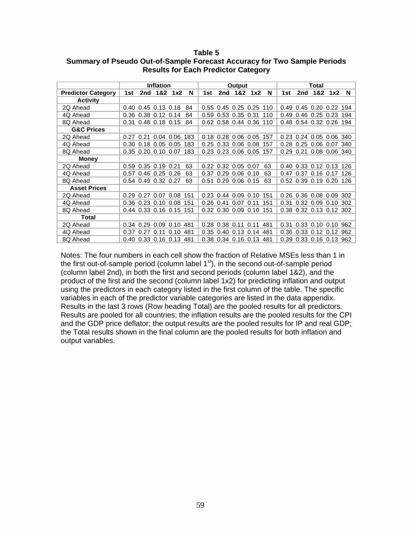
59

Table 5 Summary of Pseudo Out-of-Sample Forecast Accuracy for Two Sample Periods

Results for Each Predictor Category

Inflation Output Total Predictor Category 1st 2nd 1&2 1x2 N 1st 2nd 1&2 1x2 N 1st 2nd 1&2 1x2 N

Activity 2Q Ahead 0.40 0.45 0.13 0.18 84 0.55 0.45 0.25 0.25 110 0.49 0.45 0.20 0.22 194 4Q Ahead 0.36 0.38 0.12 0.14 84 0.59 0.53 0.35 0.31 110 0.49 0.46 0.25 0.23 194 8Q Ahead 0.31 0.48 0.18 0.15 84 0.62 0.58 0.44 0.36 110 0.48 0.54 0.32 0.26 194

G&C Prices 2Q Ahead 0.27 0.21 0.04 0.06 183 0.18 0.28 0.06 0.05 157 0.23 0.24 0.05 0.06 340 4Q Ahead 0.30 0.18 0.05 0.05 183 0.25 0.33 0.06 0.08 157 0.28 0.25 0.06 0.07 340 8Q Ahead 0.35 0.20 0.10 0.07 183 0.23 0.23 0.06 0.05 157 0.29 0.21 0.08 0.06 340

Money 2Q Ahead 0.59 0.35 0.19 0.21 63 0.22 0.32 0.05 0.07 63 0.40 0.33 0.12 0.13 126 4Q Ahead 0.57 0.46 0.25 0.26 63 0.37 0.29 0.06 0.10 63 0.47 0.37 0.16 0.17 126 8Q Ahead 0.54 0.49 0.32 0.27 63 0.51 0.29 0.06 0.15 63 0.52 0.39 0.19 0.20 126

Asset Prices 2Q Ahead 0.29 0.27 0.07 0.08 151 0.23 0.44 0.09 0.10 151 0.26 0.36 0.08 0.09 302 4Q Ahead 0.36 0.23 0.10 0.08 151 0.26 0.41 0.07 0.11 151 0.31 0.32 0.09 0.10 302 8Q Ahead 0.44 0.33 0.16 0.15 151 0.32 0.30 0.09 0.10 151 0.38 0.32 0.13 0.12 302

Total 2Q Ahead 0.34 0.29 0.09 0.10 481 0.28 0.38 0.11 0.11 481 0.31 0.33 0.10 0.10 962 4Q Ahead 0.37 0.27 0.11 0.10 481 0.35 0.40 0.13 0.14 481 0.36 0.33 0.12 0.12 962 8Q Ahead 0.40 0.33 0.16 0.13 481 0.38 0.34 0.16 0.13 481 0.39 0.33 0.16 0.13 962 Notes: The four numbers in each cell show the fraction of Relative MSEs less than 1 in the first out-of-sample period (column label 1st), in the second out-of-sample period (column label 2nd), in both the first and second periods (column label 1&2), and the product of the first and the second (column label 1x2) for predicting inflation and output using the predictors in each category listed in the first column of the table. The specific variables in each of the predictor variable categories are listed in the data appendix. Results in the last 3 rows (Row heading Total) are the pooled results for all predictors. Results are pooled for all countries; the inflation results are the pooled results for the CPI and the GDP price deflator; the output results are the pooled results for IP and real GDP; the Total results shown in the final column are the pooled results for both inflation and output variables.

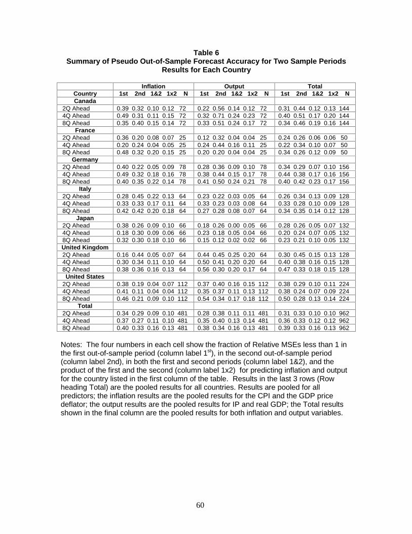
60

Table 6 Summary of Pseudo Out-of-Sample Forecast Accuracy for Two Sample Periods

Results for Each Country

Inflation Output Total Country 1st 2nd 1&2 1x2 N 1st 2nd 1&2 1x2 N 1st 2nd 1&2 1x2 N Canada

2Q Ahead 0.39 0.32 0.10 0.12 72 0.22 0.56 0.14 0.12 72 0.31 0.44 0.12 0.13 144 4Q Ahead 0.49 0.31 0.11 0.15 72 0.32 0.71 0.24 0.23 72 0.40 0.51 0.17 0.20 144 8Q Ahead 0.35 0.40 0.15 0.14 72 0.33 0.51 0.24 0.17 72 0.34 0.46 0.19 0.16 144

France 2Q Ahead 0.36 0.20 0.08 0.07 25 0.12 0.32 0.04 0.04 25 0.24 0.26 0.06 0.06 50 4Q Ahead 0.20 0.24 0.04 0.05 25 0.24 0.44 0.16 0.11 25 0.22 0.34 0.10 0.07 50 8Q Ahead 0.48 0.32 0.20 0.15 25 0.20 0.20 0.04 0.04 25 0.34 0.26 0.12 0.09 50

Germany 2Q Ahead 0.40 0.22 0.05 0.09 78 0.28 0.36 0.09 0.10 78 0.34 0.29 0.07 0.10 156 4Q Ahead 0.49 0.32 0.18 0.16 78 0.38 0.44 0.15 0.17 78 0.44 0.38 0.17 0.16 156 8Q Ahead 0.40 0.35 0.22 0.14 78 0.41 0.50 0.24 0.21 78 0.40 0.42 0.23 0.17 156

Italy 2Q Ahead 0.28 0.45 0.22 0.13 64 0.23 0.22 0.03 0.05 64 0.26 0.34 0.13 0.09 128 4Q Ahead 0.33 0.33 0.17 0.11 64 0.33 0.23 0.03 0.08 64 0.33 0.28 0.10 0.09 128 8Q Ahead 0.42 0.42 0.20 0.18 64 0.27 0.28 0.08 0.07 64 0.34 0.35 0.14 0.12 128

Japan 2Q Ahead 0.38 0.26 0.09 0.10 66 0.18 0.26 0.00 0.05 66 0.28 0.26 0.05 0.07 132 4Q Ahead 0.18 0.30 0.09 0.06 66 0.23 0.18 0.05 0.04 66 0.20 0.24 0.07 0.05 132 8Q Ahead 0.32 0.30 0.18 0.10 66 0.15 0.12 0.02 0.02 66 0.23 0.21 0.10 0.05 132 United Kingdom 2Q Ahead 0.16 0.44 0.05 0.07 64 0.44 0.45 0.25 0.20 64 0.30 0.45 0.15 0.13 128 4Q Ahead 0.30 0.34 0.11 0.10 64 0.50 0.41 0.20 0.20 64 0.40 0.38 0.16 0.15 128 8Q Ahead 0.38 0.36 0.16 0.13 64 0.56 0.30 0.20 0.17 64 0.47 0.33 0.18 0.15 128

United States 2Q Ahead 0.38 0.19 0.04 0.07 112 0.37 0.40 0.16 0.15 112 0.38 0.29 0.10 0.11 224 4Q Ahead 0.41 0.11 0.04 0.04 112 0.35 0.37 0.11 0.13 112 0.38 0.24 0.07 0.09 224 8Q Ahead 0.46 0.21 0.09 0.10 112 0.54 0.34 0.17 0.18 112 0.50 0.28 0.13 0.14 224

Total 2Q Ahead 0.34 0.29 0.09 0.10 481 0.28 0.38 0.11 0.11 481 0.31 0.33 0.10 0.10 962 4Q Ahead 0.37 0.27 0.11 0.10 481 0.35 0.40 0.13 0.14 481 0.36 0.33 0.12 0.12 962 8Q Ahead 0.40 0.33 0.16 0.13 481 0.38 0.34 0.16 0.13 481 0.39 0.33 0.16 0.13 962 Notes: The four numbers in each cell show the fraction of Relative MSEs less than 1 in the first out-of-sample period (column label 1st), in the second out-of-sample period (column label 2nd), in both the first and second periods (column label 1&2), and the product of the first and the second (column label 1x2) for predicting inflation and output for the country listed in the first column of the table. Results in the last 3 rows (Row heading Total) are the pooled results for all countries. Results are pooled for all predictors; the inflation results are the pooled results for the CPI and the GDP price deflator; the output results are the pooled results for IP and real GDP; the Total results shown in the final column are the pooled results for both inflation and output variables.

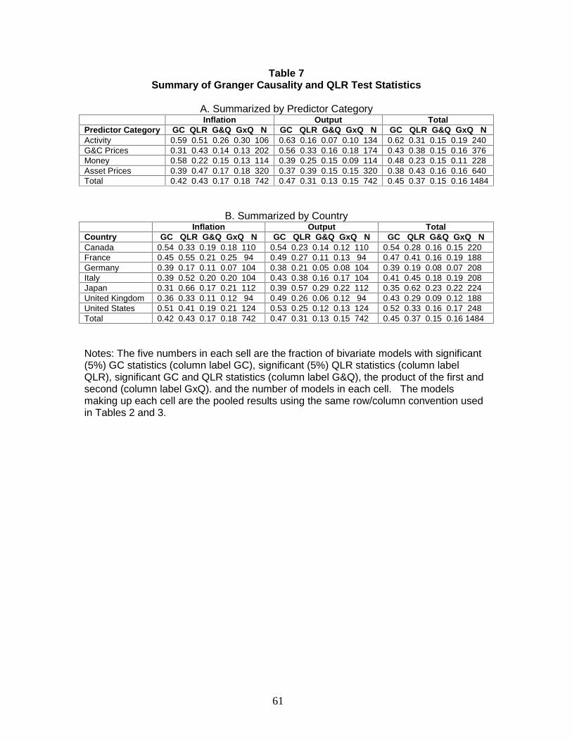
61

Table 7 Summary of Granger Causality and QLR Test Statistics

A. Summarized by Predictor Category

Inflation Output Total Predictor Category GC QLR G&Q GxQ N GC QLR G&Q GxQ N GC QLR G&Q GxQ N Activity 0.59 0.51 0.26 0.30 106 0.63 0.16 0.07 0.10 134 0.62 0.31 0.15 0.19 240 G&C Prices 0.31 0.43 0.14 0.13 202 0.56 0.33 0.16 0.18 174 0.43 0.38 0.15 0.16 376 Money 0.58 0.22 0.15 0.13 114 0.39 0.25 0.15 0.09 114 0.48 0.23 0.15 0.11 228 Asset Prices 0.39 0.47 0.17 0.18 320 0.37 0.39 0.15 0.15 320 0.38 0.43 0.16 0.16 640 Total 0.42 0.43 0.17 0.18 742 0.47 0.31 0.13 0.15 742 0.45 0.37 0.15 0.16 1484

B. Summarized by Country Inflation Output Total

Country GC QLR G&Q GxQ N GC QLR G&Q GxQ N GC QLR G&Q GxQ N Canada 0.54 0.33 0.19 0.18 110 0.54 0.23 0.14 0.12 110 0.54 0.28 0.16 0.15 220 France 0.45 0.55 0.21 0.25 94 0.49 0.27 0.11 0.13 94 0.47 0.41 0.16 0.19 188 Germany 0.39 0.17 0.11 0.07 104 0.38 0.21 0.05 0.08 104 0.39 0.19 0.08 0.07 208 Italy 0.39 0.52 0.20 0.20 104 0.43 0.38 0.16 0.17 104 0.41 0.45 0.18 0.19 208 Japan 0.31 0.66 0.17 0.21 112 0.39 0.57 0.29 0.22 112 0.35 0.62 0.23 0.22 224 United Kingdom 0.36 0.33 0.11 0.12 94 0.49 0.26 0.06 0.12 94 0.43 0.29 0.09 0.12 188 United States 0.51 0.41 0.19 0.21 124 0.53 0.25 0.12 0.13 124 0.52 0.33 0.16 0.17 248 Total 0.42 0.43 0.17 0.18 742 0.47 0.31 0.13 0.15 742 0.45 0.37 0.15 0.16 1484 Notes: The five numbers in each sell are the fraction of bivariate models with significant (5%) GC statistics (column label GC), significant (5%) QLR statistics (column label QLR), significant GC and QLR statistics (column label G&Q), the product of the first and second (column label GxQ). and the number of models in each cell. The models making up each cell are the pooled results using the same row/column convention used in Tables 2 and 3.

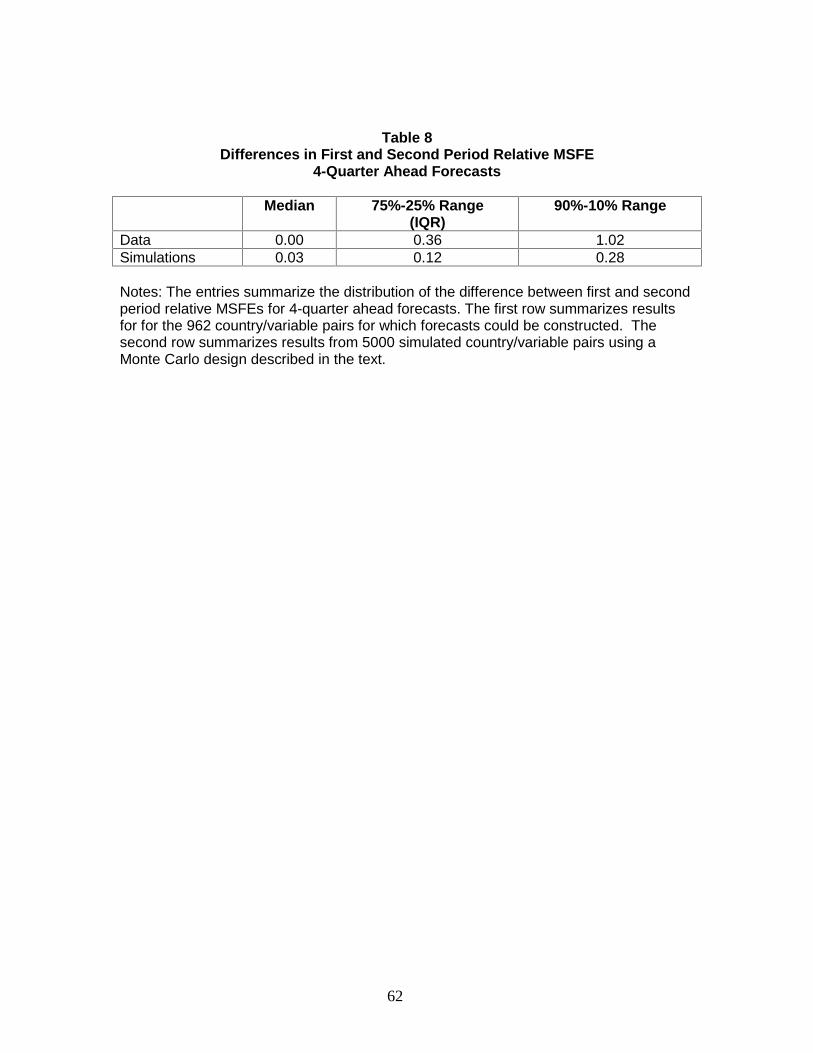
62

Table 8 Differences in First and Second Period Relative MSFE

4-Quarter Ahead Forecasts Median 75%-25% Range

(IQR) 90%-10% Range

Data 0.00 0.36 1.02 Simulations 0.03 0.12 0.28 Notes: The entries summarize the distribution of the difference between first and second period relative MSFEs for 4-quarter ahead forecasts. The first row summarizes results for for the 962 country/variable pairs for which forecasts could be constructed. The second row summarizes results from 5000 simulated country/variable pairs using a Monte Carlo design described in the text.

63

Table 9

Combined Forecasts Summary of Pseudo Out-of-Sample Forecast Accuracy for Two Sample Periods

A. GDP Deflator Canada France Germany Italy Japan U.K. U.S. 71-84 85-99 71-84 85-99 71-84 85-99 71-84 85-99 71-84 85-99 71-84 85-99 71-84 85-99 Activity 2Q Horizon 0.91 0.92 1.08 0.79 0.86 0.93 1.02 1.06 0.94 0.90 1.08 0.94 0.95 4Q Horizon 0.90 0.87 1.22 0.77 0.81 0.97 0.97 1.05 0.77 0.89 0.96 0.88 0.89 8Q Horizon 0.99 0.78 1.23 0.81 0.74 0.99 0.95 1.30 0.78 0.66 0.97 0.76 0.83 G&C Prices 2Q Horizon 1.14 0.91 0.93 1.15 1.10 0.95 0.94 0.97 1.01 0.93 0.98 1.02 1.01 4Q Horizon 1.05 0.88 0.77 0.94 1.04 0.88 0.88 0.92 1.00 0.95 1.02 0.95 0.95 8Q Horizon 1.31 0.95 0.90 1.10 0.99 0.97 1.05 0.96 0.94 0.97 0.96 0.95 0.91 Money 2Q Horizon 0.96 1.07 1.01 0.98 0.96 0.97 1.14 1.23 1.03 1.07 1.00 4Q Horizon 0.89 1.07 0.93 0.93 0.97 0.86 1.14 1.25 1.16 1.02 0.96 8Q Horizon 1.04 1.02 0.91 0.86 0.98 0.80 0.94 1.66 1.20 0.89 0.85 Asset Prices 2Q Horizon 1.04 1.02 0.92 0.97 1.02 1.01 1.02 1.04 1.09 0.98 1.03 1.15 0.93 4Q Horizon 0.93 0.96 0.92 1.02 1.02 1.02 0.98 0.95 1.11 1.07 0.95 0.96 0.87 8Q Horizon 0.81 0.90 0.86 1.06 0.97 0.85 1.01 0.87 1.04 1.00 0.81 0.78 0.81 All 2Q Horizon 0.97 0.95 0.94 0.88 0.94 0.95 0.98 1.03 0.99 0.91 0.95 1.01 0.95 4Q Horizon 0.91 0.91 0.86 0.85 0.92 0.91 0.91 0.93 0.91 0.94 0.83 0.92 0.86 8Q Horizon 0.99 0.87 0.86 0.78 0.87 0.86 0.90 0.97 0.84 0.83 0.57 0.79 0.75 Notes: Results are the relative mean square forecast errors for the combined forecasts constructed from the variables in the categories listed in the first column.

64

Table 9 (continued)

B. Consumer Price Index

Canada France Germany Italy Japan U.K. U.S. 71-84 85-99 71-84 85-99 71-84 85-99 71-84 85-99 71-84 85-99 71-84 85-99 71-84 85-99

Activity 2Q Horizon 0.97 0.90 1.02 0.92 1.00 0.90 0.91 0.99 0.94 0.92 0.79 0.75 0.88 4Q Horizon 0.96 0.77 0.95 0.82 0.91 0.89 0.90 0.99 1.07 0.82 0.77 0.72 0.82 8Q Horizon 0.90 0.60 1.35 0.66 0.76 1.03 0.93 1.07 0.97 0.66 0.66 0.71 0.69 G&C Prices 2Q Horizon 0.99 0.95 0.98 0.97 1.05 0.99 0.96 0.73 0.86 0.82 0.87 0.87 0.93 0.95 4Q Horizon 1.00 0.95 1.08 0.97 1.01 0.98 0.88 0.78 0.87 0.85 0.89 0.88 0.93 0.95 8Q Horizon 1.00 0.94 1.04 0.98 1.02 0.99 0.99 0.92 0.91 0.90 0.97 0.92 0.99 0.94 Money 2Q Horizon 0.99 1.04 1.02 1.03 0.95 0.99 0.97 0.98 1.08 0.94 0.96 0.89 4Q Horizon 0.93 1.03 1.01 0.97 0.88 0.96 0.86 0.94 0.84 1.12 0.92 0.90 8Q Horizon 0.81 1.09 0.97 0.91 0.87 0.96 0.75 0.90 0.81 1.09 0.79 0.82 Asset Prices 2Q Horizon 0.88 1.01 0.94 0.87 1.03 1.02 1.10 0.90 1.13 0.91 0.87 0.88 0.86 0.94 4Q Horizon 0.80 0.98 0.91 0.87 1.03 1.02 1.01 0.88 1.05 0.92 0.83 0.84 0.88 0.93 8Q Horizon 0.75 0.94 0.83 0.96 0.97 1.00 0.91 0.95 0.87 0.80 0.90 0.76 0.82 0.85 All 2Q Horizon 0.92 0.95 0.97 0.94 0.96 0.99 0.96 0.77 0.96 0.83 0.84 0.80 0.84 0.89 4Q Horizon 0.88 0.89 0.96 0.88 0.91 0.95 0.89 0.75 0.92 0.80 0.81 0.74 0.82 0.85 8Q Horizon 0.84 0.81 0.92 0.87 0.87 0.90 0.91 0.78 0.88 0.67 0.80 0.66 0.80 0.74 Notes: Results are the relative mean square forecast errors for the combined forecasts constructed from the variables in the categories listed in the first column.

65

Table 9 (continued)

C. Real GDP Canada France Germany Italy Japan U.K. U.S. 71-84 85-99 71-84 85-99 71-84 85-99 71-84 85-99 71-84 85-99 71-84 85-99 71-84 85-99 Activity 2Q Horizon 0.97 0.90 1.03 1.03 0.94 0.95 0.88 0.98 0.97 1.01 0.89 0.93 0.99 4Q Horizon 1.03 0.97 1.12 0.95 0.93 1.01 0.75 1.01 0.94 1.10 0.98 0.98 1.01 8Q Horizon 1.03 0.99 0.95 1.06 0.94 1.08 0.72 0.98 0.96 1.04 1.16 1.02 1.00 G&C Prices 2Q Horizon 1.07 1.03 1.09 1.01 1.02 1.06 1.02 0.94 1.02 1.01 0.95 0.94 1.05 4Q Horizon 1.01 1.06 1.13 0.92 1.15 0.88 1.24 1.05 1.03 0.95 0.94 0.92 1.10 8Q Horizon 0.97 1.05 1.03 0.93 1.07 0.81 1.07 1.00 1.02 0.99 0.96 0.83 1.09 Money 2Q Horizon 0.91 0.79 0.97 0.98 0.99 0.85 0.76 0.64 0.92 0.85 1.02 4Q Horizon 0.94 0.81 0.99 0.92 0.96 0.83 0.65 0.67 0.87 0.83 0.93 8Q Horizon 0.95 0.83 0.90 1.00 0.91 0.87 0.58 0.91 0.84 0.88 0.89 Asset Prices 2Q Horizon 0.90 0.76 1.01 0.78 0.98 0.92 1.00 0.90 0.94 1.04 0.95 0.81 0.94 4Q Horizon 0.85 0.76 1.04 0.67 1.04 0.82 0.93 1.05 0.90 0.79 0.99 0.71 1.01 8Q Horizon 0.77 0.74 0.98 0.81 0.99 0.82 0.74 1.27 0.94 0.72 1.07 0.58 0.98 All 2Q Horizon 0.93 0.85 0.97 0.91 0.96 0.91 0.87 0.89 0.94 1.01 0.92 0.86 0.96 4Q Horizon 0.94 0.89 1.02 0.84 0.99 0.85 0.82 0.99 0.91 0.88 0.96 0.83 0.98 8Q Horizon 0.92 0.90 0.92 0.94 0.96 0.87 0.75 1.05 0.92 0.87 1.05 0.79 0.97 Notes: Results are the relative mean square forecast errors for the combined forecasts constructed from the variables in the categories listed in the first column.

66

Table 9 (continued)

D. Industrial Production Canada France Germany Italy Japan U.K. U.S. 71-84 85-99 71-84 85-99 71-84 85-99 71-84 85-99 71-84 85-99 71-84 85-99 71-84 85-99 Activity 2Q Horizon 1.00 0.94 0.86 0.92 0.98 1.01 0.80 0.96 0.96 1.03 0.84 0.96 0.94 4Q Horizon 0.98 1.01 0.90 0.98 1.02 1.00 0.62 0.98 0.92 0.97 0.86 0.97 1.00 8Q Horizon 1.00 1.02 0.91 1.11 1.00 0.96 0.76 0.95 0.93 0.97 0.96 1.02 0.98 G&C Prices 2Q Horizon 0.99 1.06 0.89 1.18 0.85 1.04 0.93 1.00 0.83 1.08 0.93 0.95 0.95 1.10 4Q Horizon 0.92 1.12 0.89 1.25 0.84 1.15 0.94 1.16 0.82 1.13 0.83 0.99 0.91 1.13 8Q Horizon 0.90 1.08 0.99 1.11 0.89 1.06 1.17 1.12 0.95 1.08 0.96 1.02 0.81 1.02 Money 2Q Horizon 0.96 0.93 0.98 1.03 0.92 0.99 0.82 0.84 0.99 0.86 0.83 1.01 4Q Horizon 0.89 0.92 1.00 1.01 0.88 0.92 0.84 0.69 1.13 0.70 0.76 0.99 8Q Horizon 0.94 0.81 0.95 1.00 0.93 0.88 1.04 0.55 0.53 0.66 0.82 0.97 Asset Prices 2Q Horizon 0.84 0.92 0.79 0.96 0.82 0.96 0.94 0.93 0.89 0.96 1.03 0.88 0.78 0.94 4Q Horizon 0.79 0.81 0.82 0.96 0.75 0.89 0.94 0.83 0.95 0.91 0.95 0.90 0.58 0.95 8Q Horizon 0.75 0.71 0.87 0.94 0.79 0.85 0.75 0.76 1.09 0.77 0.72 0.94 0.44 0.86 All 2Q Horizon 0.93 0.93 0.86 0.95 0.86 0.97 0.92 0.86 0.88 0.94 0.98 0.87 0.85 0.94 4Q Horizon 0.88 0.93 0.86 0.96 0.84 0.97 0.92 0.75 0.89 0.88 0.89 0.89 0.76 0.96 8Q Horizon 0.88 0.88 0.91 0.93 0.92 0.92 0.93 0.75 0.94 0.83 0.82 0.94 0.72 0.91 Notes: Results are the relative mean square forecast errors for the combined forecasts constructed from the variables in the categories listed in the first column.