30

Forecasting leptospirosis incidence in the Philippines using the Box–

Jenkins method

*John Mark Alcaria, Anthony Capili

Mathematics and Statistics Department, University of Southeastern Philippines, Davao City

*Corresponding author: alcaria_johnmark@yahoo.com

Date received: October 10, 2020

Date accepted: December 16, 2020

Date published: December 30, 2020

ABSTRACT

This study aims to investigate and find a suitable model for forecasting the leptospirosis

incidence in the Philippines. The Box-Jenkins approach was utilized in the development of an

appropriate model. The dataset was retrieved from the Epidemiology Bureau of the Department

of Health containing the weekly number of leptospirosis cases in the Philippines from 2016 to

2018. This dataset was analyzed using the R software. The original series is nonstationary with

indications of nonconstant variance. Box-Cox transformation and ordinary differencing were

performed on the series. The transformed series was analyzed and the results show that

ARIMA(0,1,0) or the random walk model is the most appropriate model for forecasting

leptospirosis incidence. The residuals and forecast errors of the fitted model behave like a white

noise process. The fitted model may be used for forecasting the future number of leptospirosis

cases in the Philippines.

Keywords: forecasting, Box-Jenkins method, leptospirosis, randow walk, epidemiology,

Philippines.

INTRODUCTION

Leptospirosis is a bacterial disease that affects humans and animals. It is caused by bacteria of

the genus Leptospira. Leptospira is a spiral-shaped Gram-negative spirochete with internal

flagella, which enters the host through mucosa and broken skin. Without treatment,

leptospirosis can lead to kidney damage, meningitis (inflammation of the membrane around

the brain and spinal cord), liver failure, respiratory distress, and even death (Centers for Disease

Control and Prevention, 2017).

Leptospirosis are found throughout the world, but prevalence is higher in tropical regions with

high rain fall (Haake & Levett 2015). Leptospirosis is a major public health concern,

particularly in developing countries with limited economic resources. However, recent reports

indicated its emergence as an important health risk in developed and developing countries

including European countries, especially among individuals participating in water sport

activities (Dupouey et al., 2014; Haake et al., 2002).

Very little is currently known regarding the true incidence of leptospirosis. It is estimated that

0.1 to 1 per 100,000 people living in temperate climates are affected each year, with the number

increasing to 10 or more per 100,000 people living in tropical climates. If there is an epidemic,

31

the incidence can soar to 100 or more per 100,000 people (World Health Organization, 2018).

In the Philippines, leptospirosis incidence tend to be frequent in flood-prone areas of urban

setting such as Metro Manila. From 1998 to 2001, about 70% of 1200 suspected leptospirosis

patients in Philippines were tested positive for the disease. The average age of patients was 32

years old. Around 87% of the cases were males and 70% were outdoor workers. Case fatality

rate was found to be 12 to 14% (Villanueva et al., 2007).

In the Philippines, a total of 2,495 leptospirosis cases were reported nationwide in 2017. This

is 49.1% higher compared to 1,673 cases in 2016. Most of the cases were from the National

Capital Region (NCR), Region VI, Region I, Region III and Region II (Department of Health,

2017). In response to this problem, the Department of Health coordinated with the College of

Public Health (CPH) of the University of the Philippines and employed preventions called

Leptospirosis Control (LepCon). They have conducted seminars and lectures in every

barangays in Quezon City for preventions and disease planning management. In addition, DOH

visits various elementary schools and conducts nationwide advocacy activities, lectures, and

awareness programs on leptospirosis.

Over the past years, several studies have been conducted on leptospirosis incidence. The Box-

Jenkins method is one of the usual techniques used in forecasting leptospirosis incidence. This

method is commonly used because of its applicability on seasonal time series. Seasonal

Autoregressive Integrated Moving Average (SARIMA) models have been used in different

studies (Chadsuthi et al., 2012; Gnanapragasam, 2017; Phrom, 2012) but there are also

instances where the Autoregressive Integrated Moving Average (ARIMA) model was utilized

(Ap, 2015).

This study aims to investigate and find a suitable ARIMA model for forecasting Leptospirosis

incidence in the Philippines. The model shall be developed using the Box-Jenkins approach.

Box-Jenkins Method

The Box-Jenkins approach is a systematic method of time series model development that

involves the stages of model identification, parameter estimation, and diagnostic checking. The

models that are presented in the succeeding sections were taken from the books of Adhikari

and Agrawal (2009) and Montgomery, Jennings and Kulachi (2008).

Autoregressive models are as their name suggests-regressions on themselves. The future value

of a variable is assumed to be a linear combination of p past observations and a random error

together with a constant term. An autoregressive model of order p, denoted by AR(p), is given

by

𝑦𝑡 = 𝑐 + ∑ 𝜑𝑖𝑦𝑡−𝑖

𝑝

𝑖=1

+ є𝑡

(1)

where 𝑦𝑡 and є𝑡 are respectively the actual value and random error (or random shock) at time

period t, 𝜑𝑖 (𝑖 = 1,2, . . , 𝑝) are model parameters and c is a constant. The random shock is

assumed to be a white noise process.

32

If the future value of a variable is a linear combination of present and past random shocks, we

have what is called a moving average. The moving average model of order q, denoted by

MA(q), is given by

𝑦𝑡 = 𝜇 + ∑ θjєt−j

q

j=1

+ є𝑡

(2)

where 𝜇 is the mean of the series, 𝜃𝑗 (𝑗 = 1,2, … 𝑞) are the model parameters.

If we assume that the series is partly autoregressive and partly moving average, we obtain a

quite general time series model. An autoregressive moving average model of order p and q,

denoted by ARMA(p, q) is given by

𝑦𝑡 = 𝑐 + є𝑡 + ∑ 𝜑𝑖𝑦𝑡−𝑖

𝑝

𝑖=1

+ ∑ 𝜃𝑗є𝑡−𝑗

𝑞

𝑗=1

(3)

we say that {𝑦𝑡} is a mixed autoregressive moving average process of orders p and q,

respectively.

The autoregressive integrated moving average model is capable of representing a non-

stationary time series. An autoregressive integrated moving average model of order p, d, and

q, denoted by ARIMA(p,d,q) is given by

𝜑 𝑝(𝐿)(1 − 𝐿)𝑑𝑦𝑡 = 𝜃𝑞(𝐿)𝜖𝑡

(4)

where p, d and q are integers greater than or equal to zero and refer to the order of the

autoregressive, integrated, and moving average parts of the model respectively, L is the

backward shift operator and the integer d controls the level of differencing. The backshift

operator is a notational device that shifts the data back into a specific number of periods. That

is, for the backshift notation 𝐿 then 𝐿𝑑𝑦𝑡 = 𝑦𝑡−𝑑. In addition, 𝜑 𝑝(𝐿) = 1 − ∑ 𝜑𝑖𝑝𝑖=1 𝑦𝑡−𝑖 and

𝜃𝑞(𝐿) = 1 + ∑ 𝜃𝑗𝜖𝑡−𝑗 .𝑞𝑗=1

When the data is affected by seasonality, a Seasonal ARIMA model

SARIMA(p,d,q)×(P,D,Q)𝑆 , where 𝑃, 𝐷, and 𝑄 are the order of the autoregressive,

differencing, and moving average for the seasonal component and S is the seasonal length. The

mathematical formulation of a SARIMA(p,d,q)×(P,D,Q)𝑆 model in terms of backshift notation

is given by

𝛷𝑃 (𝐿𝑠)𝜑𝑝(𝐿)(1 − 𝐿)𝑑(1 − 𝐿𝑠)𝐷𝑦𝑡 = 𝛩𝑄(𝐿𝑠)𝜃𝑞(𝐿)𝜖𝑡

(5)

where 𝛷𝑃(𝐿𝑆) = 1 − ∑ Φ𝑖𝑃𝑖=1 𝐿𝑆𝑖 and 𝛩𝑄(𝐿𝑆) = 1 + ∑ 𝛩𝑗

𝑄𝑗=1 𝐿𝑆𝑗 .

33

The random walk process, ARIMA (0, 1, 0) is the simplest nonstationary model. The model is

given by

(1-𝐿)𝑦𝑡 = 𝑐 + 𝜖𝑡 (6)

In a random walk model, the autocorrelation and partial autocorrelation of the first difference

of 𝒚𝒕 should not be significant. In other words, differencing of the original series eliminates all

serial dependence and yields a white noise process.

Table 1 shows the behavior of the autocorrelation and partial autocorrelation (ACF/PACF)

functions of an ARMA process (Montgomery, Jennings & Kulahci, 2008).

Table 1. ACF and PACF of ARMA Models

MA(q) AR(p) ARMA (p,q)

ACF cuts off after lag q

exponential decay

and/or damped

sinusoid

exponential decay

and/or damped sinusoid

PACF exponential decay

and/or damped sinusoid cuts off after lag p

exponential decay

and/or damped sinusoid

The theoretical ACF and PACF of SARIMA Models may be used for identifying seasonal

components. The behavior of the ACF and PACF of SARIMA models are shown in Table 2

(Shumway & Stoffer, 2000).

Table 2. ACF and PACF of SARIMA Models

AR(P)𝑠 MA(Q)𝑠 ARMA (P,Q)𝑠

ACF Tails off at lag ks,

k=1,2,…, Cuts off after lag Qs

Tails off at lag ks,

k=1,2,…,

PACF Cuts off after lag Ps

Tails off at lag ks, k=

1,2,…,

Tails off at lag ks,

k= 1,2,…,

METHOD

The data was obtained from the Department of Health (DOH) website, specifically, from the

agency’s Leptospirosis Surveillance Report. It is composed of weekly number of Leptospirosis

cases in the Philippines (1st week of January 2016 ¬– 4th week of December 2018) where 130

data points (1st week of January 2016 – 4th week of June 2018) were used in model building

and 26 data points (1st week of July 2018 to 4th week of December 2018) for the forecast

evaluation. This dataset contains reported cases only. Considering the possibility of unreported

cases, actual leptospirosis incidences may be higher than the reported cases. This study is

limited to the analysis of reported cases and unreported cases were not included.

34

According to Montgomery, Jennings and Kulahci (2008), the Box-Jenkins approach is

composed of three stages, namely, model identification, parameter estimation, and diagnostic

checking. An additional step on forecasting evaluation is also recommended and the entire

procedure is as follows:

1. Model Identification. In this stage, a time series plot shall be constructed. The plot will be

used as a tool for the preliminary assessment of stationarity. If non-stationarity is suspected

(i.e. there is a trend, seasonality and/or nonconstant variance), differencing and other

methods of transformation may be applied. A stationarity test may be performed in order

to formally check the stationarity of the series. Once the stationarity can be assumed, the

sample autocorrelation and partial autocorrelation functions (ACF/PACF) should be

obtained. Tentative models shall be identified based on ACF and PACF plots. The model

with the least Akaike’s Information Criterion value shall be selected.

2. Model Estimation. The parameters of the selected model shall be estimated. By default, R

uses a combination of conditional sum of squares and maximum likelihood in the

estimation process.

3. Diagnostic Checking. Residual analysis shall be conducted on the fitted model. The Ljung-

Box Test will be used to test if the model is a good to fit to the series. In the addition, ACF

and PACF plots of the residuals shall be generated. The fitted model is inadequate if there

is a lack of fit, spikes on the ACF/PACF plots, and/or patterns in the residual plots. In such

cases, the researcher should go back to the model identification stage and identify a new

model.

4. Forecast Evaluation. The estimated model will be used to generate one-step ahead

forecasts of the out-sample dataset. This data refers to the observations that were not used

for model identification and estimation. Ideally, the forecast errors should behave like a

Gaussian white noise process. The ACF and PACF plots of the forecast errors shall be

generated. In addition, Shapiro Wilk test will be performed on these errors. If the forecast

errors are Gaussian white noise, there should be no spikes in the ACF and PACF plots.

Furthermore, the normality test should not yield a significant result.

This study made use of the following packages: forecast for model estimation and forecasting;

tseries for testing of stationarity; astsa for generating ACF and PACF plots; stats for the Ljung

Box Test; and lmtest for checking the parameter significance. All the packages are available in

the R software.

RESULTS

Figure 1 shows the time series plot of the weekly number of Leptospirosis cases in the

Philippines. The time series data is composed of 130 weekly observations from 1st week of

January 2016 to 4th week of June 2018. Generally, the plot exhibits changing levels with no

apparent seasonality. In addition, the series seems to have a non-constant variance. That is, the

variability from the 1st week of January 2016 to 4th week of June 2016 and 1st week of January

2017 to 4th week of June 2017 appears to be smaller than the other weekly periods.

35

Figure 1. Time Series Plot of Leptospirosis Incidence

In order to correct the problem of variability, the series was subjected to a Box Cox

transformation. An optimal lambda of -0.0834 was used in the said transformation. Figure 2

shows the time series plot of the transformed series. The transformed series seems to change

levels, an indication of non-stationarity.

Figure 2. Time Series Plot of the Transformed Series

To formally test the stationarity of the series, the ADF test was used. Table 4 displays the ADF

test statistic and its p-value. Since the p-value is larger than the 0.05 level of significance, the

null hypothesis of non-stationarity cannot be rejected. The evidence is not enough to conclude

that the transformed series is stationary.

Table 3. ADF Test for Stationarity of the Transformed Series

ADF Test Statistic p-value

-2.4056 0.4079

36

To make the series stationary, first order differencing was applied to the transformed series and

the resulting series is shown in Figure 3. It can be observed that the data points are generally

oscillating randomly around a constant mean. This behavior is consistent with the behavior of

a stationary series.

Figure 3. Time Series Plot of the First Difference

To formally test the stationarity of the differenced series, the ADF test was performed. Table

4 displays the ADF test statistic and its p-value. Since the p-value is lower than 0.01, the null

hypothesis can be rejected. Hence, the first difference is stationary.

Table 4. ADF Test for Stationarity of the First Difference

ADF Test Statistic p-value

-4.6964 <0.01

The ACF and PACF plots of the first difference have no significant spikes. This is the behavior

of a white noise process. Since the resulting series is possibly white noise after first

differencing, the transformed series may be modelled using a random walk process. Thus,

ARIMA (0, 1, 0) or the random walk model is chosen for the transformed series.

37

Figure 4. ACF and PACF of the First Difference

The random walk model or ARIMA (0, 1, 0) has no estimated autoregressive and moving

average parameters.

To check if there is another model with an AIC value lower than the chosen model, the process

of overfitting was performed. Table 5 shows the overfitted models and their corresponding AIC

values. There are two models with AIC values that are lower than the chosen model. These

models are ARIMA (0, 1, 1) and ARIMA (0, 1, 2).

Table 5. Overfitted Models

Model AIC

ARIMA (0, 1, 0)

ARIMA (1, 1, 0)

79.38

79.68

ARIMA (2, 1, 0) 79.88

ARIMA (0, 1, 1) 79.07

ARIMA (0, 1, 2) 78.75

Table 6 shows the parameter estimates of ARIMA (0, 1, 2). The estimated MA(1) parameter

has a p-value of 0.0607 which is significant at a 0.10 level of significance. However, the

estimated MA(2) parameter has a large p-value of 0.1220, therefore this parameter is not

significant.

Table 6. Parameter Estimates of ARIMA (0, 1, 2) Model

Parameter Estimate S.E. z value p-value

MA(1) -0.1794 0.0956 -1.8760 0.0607

MA(2) -0.1508 0.0975 -1.5464 0.1220

38

Table 7 shows the parameter estimate of ARIMA (0, 1, 1), its z value and p-value. The

estimated parameter is not significant with a large p-value of 0.1331. Both overfitted models

have nonsignificant parameters. Thus, the final model is ARIMA (0, 1, 0). The adequacy of the

chosen model was examined through a residual analysis.

Table 7. Parameter Estimates of ARIMA (0, 1, 1) Model

Parameter Estimate Standard Error z value p-value

MA(1) -0.1707 0.1137 -1.5021 0.1331

Figure 5 shows the residual plots of the chosen model. The plot of the residuals versus fitted

values exhibit random behavior. Thus, the residuals seem to have a constant variance. The same

random behavior can be observed when the residuals are plotted against time. This is an

indication of uncorrelated residuals. Lastly, the normal probability plot of residuals shows

severe deviations from normality. That is, some points are far from theoretical line.

39

Figure 5. Residual Plots

Figure 6 shows the ACF and PACF plots of the residuals. The autocorrelations and partial

autocorrelations are within the maximum and minimum limits as represented by the blue

fragmented lines in the plots. Thus, individually, there are no significant autocorrelations and

partial autocorrelations among the residuals.

Figure 6. ACF and PACF of the Residuals

To formally test the presence of a serial autocorrelation over several lags, the Ljung-Box Test

was performed. Table 8 shows the Ljung-Box test statistic with its degrees of freedom and p-

value. Since the p-value of 0.9032 is greater than 0.05, the null hypothesis of no serial

autocorrelation cannot be rejected. The statistical evidence does not support the existence of

autocorrelated residuals. Given the previous results, it is reasonable to conclude that the

residuals were generated by a white noise process.

Table 8. Ljung-Box Test for Residuals

Test Statistic Degrees of Freedom p-value

12.3590 20 0.9032

40

Table 9 contains the actual data from the 1st week of July 2018 to 4th week of December 2018,

one-step ahead forecast values, and forecast errors. The model’s performance was evaluated

using these forecast errors.

Table 9. One-Step Ahead Forecast and Forecast Errors

Week Date Actual Forecast Forecast

Error

Week 27 July 01 - July 07, 2018 180 375 -195

Week 28 July 08 - July 14, 2018 151 180 -29

Week 29 July 15 - July 21, 2018 160 151 9

Week 30 July 22 - July 28, 2018 193 160 33

Week 31 July 29 - Aug. 04, 2018 385 193 192

Week 32 Aug. 05 - Aug. 11, 2018 310 385 -75

Week 33 Aug. 12 - Aug. 18, 2018 180 310 -130

Week 34 Aug. 19 - Aug. 25, 2018 295 180 115

Week 35 Aug. 26 - Sept 01, 2018 326 295 31

Week 36 Sept. 02 - Sept. 08, 2018 178 326 -148

Week 37 Sept. 09 - Sept. 15, 2018 120 178 -58

Week 38 Sept.16 - Sept. 22, 2018 139 120 19

Week 39 Sept. 23 - Sept. 29, 2018 178 139 39

Week 40 Sept. 30 - Oct. 06, 2018 174 178 -4

Week 41 Oct. 07 - Oct. 13, 2018 102 174 -72

Week 42 Oct. 14 - Oct. 20, 2018 127 102 25

Week 43 Oct. 21 - Oct. 27, 2018 67 127 -60

Week 44 Oct. 28 - Nov. 03, 2018 58 67 -9

Week 45 Nov. 04 - Nov. 10, 2018 59 58 1

Week 46 Nov. 11 - Nov. 17, 2018 45 59 -14

Week 47 Nov. 18 - Nov. 24, 2018 42 45 -3

Week 48 Nov. 25 - Dec. 01, 2018 38 42 -4

Week 49 Dec. 02 – Dec. 08, 2018 42 38 4

Week 50 Dec. 09 – Dec. 15, 2018 31 42 -11

Week 51 Dec. 16 – Dec. 22, 2018 23 31 -8

Week 52 Dec. 23 – Dec. 31, 2018 16 23 -7

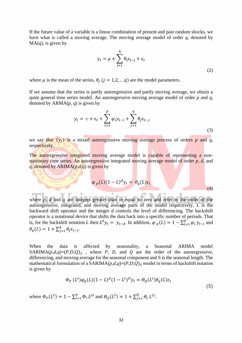
Figure 7 displays the ACF and PACF plots of the forecast errors. Most of the autocorrelations

and partial autocorrelations are not significant. However, in both plots there is a small spike at

lag 2. This is still an indication of uncorrelated residuals.

41

Figure 7. ACF and PACF Plots of the Forecast Errors

Table 10 shows the results of the Shapiro-Wilk test. Since the p-value of 0.0058 is lower than

0.05, the forecast errors are not normally distributed. Finally, given the previous results, the

residuals behave like a white noise process.

Table 10. Shapiro-Wilk Test of Normality

Test Statistic p-value

0.8803 0.0058

Table 11 shows the forecasted values for the 1st week of January 2019 to the 4th week of June

2019. The 95% confidence limits are also shown in the table.

42

Table 11. Forecasted Values

CONCLUSION

The weekly incidence of leptospirosis from the 1st week of January 2016 to the 4th week of

June 2018 showed changing levels with no clear seasonality. The series exhibits a non-constant

variance. The random walk model or ARIMA (0, 1, 0) is the chosen model for Leptospirosis

incidence. The model is given by

(1-𝐵)𝑦𝑡′ = 𝜖𝑡

where

𝑦𝑡′= the series after Box Cox transformation

Overfitting was performed on ARIMA (0, 1, 0). However, the other models with lower AIC

values have nonsignificant parameters. Thus, ARIMA (0, 1,0) is the final model.

Week Date Forecast 95% Confidence Limit

Lower Upper

Week 1 Jan. 01 - Jan. 05, 2019 16 7.3292 36.8818

Week 2 Jan. 06 - Jan. 12, 2019 16 5.3807 53.0608

Week 3 Jan. 13 - Jan. 19, 2019 16 4.2672 70.6834

Week 4 Jan. 20 - Jan, 26, 2019 16 3.5216 90.5062

Week 5 Jan. 27 - Feb. 02, 2019 16 2.9809 113.0148

Week 6 Feb. 03 - Feb. 09, 2019 16 2.5690 138.6450

Week 7 Feb. 10 - Feb. 16, 2019 16 2.2442 167.8393

Week 8 Feb. 17 - Feb. 23, 2019 16 1.9816 201.0692

Week 9 Feb. 24 - Mar. 02, 2019 16 1.7651 238.8480

Week 10 Mar. 03 - Mar. 09, 2019 16 1.5837 281.7402

Week 11 Mar. 10 - Mar. 16, 2019 16 1.4298 330.3696

Week 12 Mar. 17 - Mar, 23 2019 16 1.2978 385.4275

Week 13 Mar. 24 - Mar. 30, 2019 16 1.1835 447.6807

Week 14 Mar. 31 - Apr. 06, 2019 16 1.0838 517.9810

Week 15 Apr. 07 - Apr. 13, 2019 16 0.9961 597.2746

Week 16 Apr. 14 - Apr. 20, 2019 16 0.9186 686.6128

Week 17 Apr. 21 - Apr. 27, 2019 16 0.8497 787.1640

Week 18 Apr. 28 - May 04, 2019 16 0.7881 900.2267

Week 19 May 05 - May 11, 2019 16 0.7328 1027.2443

Week 20 May 12 - May 18, 2019 16 0.6830 1169.8209

Week 21 May 19 - May 25, 2019 16 0.6379 1329.7394

Week 22 May 26 - Jun. 01, 2019 16 0.5970 1508.9814

Week 23 Jun. 02 - Jun. 08, 2019 16 0.5597 1709.7495

Week 24 Jun. 09 - Jun. 15, 2019 16 0.5257 1934.4918

Week 25 Jun. 16 - Jun. 22, 2019 16 0.4950 2185.9297

Week 26 Jun. 23 - Jun. 29, 2019 16 0.4659 2467.0881

43

Based on the ACF and PACF plots, the autocorrelation and partial autocorrelation values of

the residuals are within acceptable limits. The plot of residuals versus fitted values and

residuals versus time are structureless. In addition, some of the residuals are far from the

theoretical line of normality. Finally, the result of the Ljung-Box test does not support the

existence of autocorrelated residuals. Thus, the residuals are generated by a white noise

process.

The autocorrelation and partial autocorrelation values of the forecast errors are significant at

lag 2. Still, most of the ACF and PACF values are not significant. The result of the Shapiro-

wilk test is significant. Hence, the forecast errors generally behave like a white noise process.

The forecasted values for the 1st week of January 2019 to the 4th week of June 2019 is 16 cases.

This forecast should be updated whenever new data becomes available.

REFERENCES

Adhikari, R., & Agrawal, R. (2013). An introductory study on time series and forecasting. Germany:

Lambert Academic Publishing.

Ap, T. (2015). Forecasting of leptospirosis case in Yogyakarta city using time series method and time

series combination with Bayesian network. Retrieved August 18, 2018 from

http://etd.repository.ugm.ac.id/index.php?mod=penelitian_detail&sub=PenelitianDetail&act=vi

ew&typ=html&buku_id=89586&obyek_id=4

Centers for Disease Control and Prevention. (2017). About leptospirosis. Retrieved August 18, 2018

from https://www.cdc.gov/malaria/about/index.hTml

Chadsuthi et al. (2012). Modeling seasonal leptospirosis transmission and its association with rainfall

and temperature in Thailand using time-series and ARIMAX analyses. Asian Pacific Journal of

Tropical Medicine, 5(7), 539-546.

Cryer, J. D., & Chan, K.-S. (2008). Time series analysis with applications in R. New York: Springer

Science Business Media, LLC.

Department of Health. (2016, December 31). Leptospirosis surveillance report. Retrieved August 18,

2018, from https://www.doh.gov.ph/sites/default/files/statistics/Lep tospirosis_MW1-

MW52_2016.pdf

Department of Health. (2017, December 2). Leptospirosis surveillance report. Retrieved August 18,

2018, from https://www.doh.gov.ph/sites/default/files/statistics/DSR-LEPTOSPIROSIS-MW1-

MW48.pdf

Eftimie, N. (2017). Method of using the box-cox transformation at the application of the xbar and s

chart. Retrieved from https://doi.org/10.1051/matecconf/2 0179 404005

Gnanapragasam, S.R. (2017). An empirical study on human leptospirosis cases in the western province

of Sri Lanka. Open University of Sri Lanka Journal, 12(1), 109-127

Montgomery, D. C., Jennings, C. L., & Kulachi, K. (2008). Time series analysis and forecasting.

Hoboken: John Wiley & sons, Inc.

44

Natrella, M. (2012, April). Box-ljung test. Retrieved October 6, 2018, from Engineering Statistics

Handbook: http://www.itl.nist.gov/div898/handbook /pmc/section4/pmc4481.htm

Natrella, M. (2015, July 14). Retrieved October 6, 2018, from Box Cox Transformation:

http://www.statisticshowto.com/box-cox-transformation/

Natrella, M. (2012, April). Anderson-darling and shapiro wilk test. Retrieved October 6, 2018, from

Engineering Statistics Handbook: http://www.

itl.nist.gov/div898/handbook/prc/section2/prc213.htm

Phrom, M. (2012). Forecasting of leptospirosis transmission in Sakon Nakhon Province: SNRU Journal

of Science and Technology, 4 (7), 23-34.

Stata Corp LLC (n.d). dfuller. Augmented dickey fuller unit root. Retrieved: October 6, 2018 from

stata.com.https://www. stata.com /manuals13

Stoffer, D. (2017). astsa: Applied statistical time series analysis. Retrieved October 14, 2018, from R

Package Version 1.8: https://CRAN.Rproject.org/p ackage=astsa

Team, R. C. (2016). R: A language and environment for statistical computing. Retrieved October 14,

2018, from R Foundation for Statistical Computing Web site: htttps://.R-project.org/

Trapletti, A., & Hornik, K. (2017). tseries: Time series analysis and computational Finance. Retrieved

October 14, 2018, from R Version Packages 0.10-42: https://CRAN.R-

project.org/package=tseries

Villanueva et al. (2007). Current status of leptospirosis in Japan and Philippines. Comparative

Immunology, Microbiology and Infectious Diseases Journal, 30(5-6), 399-413.

World Health Organization (2018). About leptospirosis. Retrieved September 29, 2018, from

http://www.who.int/topics/leptospirosis/en/

World Health Organization (2018). About leptospirosis. Retrieved September 29, 2018, from

http://www.who.int/zoonoses/diseases/leptospirosis/en/