force field benchmark of organic liquids: density...

Published: December 07, 2011

r 2011 American Chemical Society 61 dx.doi.org/10.1021/ct200731v | J. Chem. Theory Comput. 2012, 8, 61–74

ARTICLE

pubs.acs.org/JCTC

Force Field Benchmark of Organic Liquids: Density, Enthalpy ofVaporization, Heat Capacities, Surface Tension, Isothermal Com-pressibility, Volumetric Expansion Coefficient, and Dielectric ConstantCarl Caleman,† Paul J. van Maaren,‡ Minyan Hong,‡ Jochen S. Hub,‡ Luciano T. Costa,§ andDavid van der Spoel*,‡

†Center for Free-Electron Laser Science, Deutsches Elektronen-Synchrotron Notkestraße 85, DE-22607 Hamburg, Germany‡Department of Cell and Molecular Biology, Uppsala University, Husargatan 3, Box 596, SE-75124 Uppsala, Sweden§Departamento de Ciencias Exatas, Federal University of Alfenas—MG Rua Gabriel Monteiro da Silva, 700 Alfenas—MG CEP:37130-000, Brazil

bS Supporting Information

ABSTRACT: The chemical composition of small organic molecules is often very similar to amino acid side chains or the bases innucleic acids, and hence there is no a priori reason why amolecular mechanics force field could not describe both organic liquids andbiomolecules with a single parameter set. Here, we devise a benchmark for force fields in order to test the ability of existing forcefields to reproduce some key properties of organic liquids, namely, the density, enthalpy of vaporization, the surface tension, the heatcapacity at constant volume and pressure, the isothermal compressibility, the volumetric expansion coefficient, and the staticdielectric constant. Well over 1200 experimental measurements were used for comparison to the simulations of 146 organic liquids.Novel polynomial interpolations of the dielectric constant (32 molecules), heat capacity at constant pressure (three molecules), andthe isothermal compressibility (53molecules) as a function of the temperature have beenmade, based on experimental data, in orderto be able to compare simulation results to them. To compute the heat capacities, we applied the two phase thermodynamicsmethod(Lin et al. J. Chem. Phys. 2003, 119, 11792), which allows one to compute thermodynamic properties on the basis of the density ofstates as derived from the velocity autocorrelation function. The method is implemented in a new utility within the GROMACSmolecular simulation package, named g_dos, and a detailed expos�e of the underlying equations is presented. The purpose of thiswork is to establish the state of the art of two popular force fields, OPLS/AA (all-atom optimized potential for liquid simulation) andGAFF (generalized Amber force field), to find common bottlenecks, i.e., particularly difficult molecules, and to serve as a referencepoint for future force field development. To make for a fair playing field, all molecules were evaluated with the same parametersettings, such as thermostats and barostats, treatment of electrostatic interactions, and system size (1000 molecules). The densitiesand enthalpy of vaporization from an independent data set based on simulations using the CHARMM General Force Field(CGenFF) presented by Vanommeslaeghe et al. (J. Comput. Chem. 2010, 31, 671) are included for comparison.We find that, overall,the OPLS/AA force field performs somewhat better than GAFF, but there are significant issues with reproduction of the surfacetension and dielectric constants for both force fields.

1. INTRODUCTION

Parameters in most force fields have been derived incrementally,that is, building on previous work by adding support for differentchemical moieties in a sequential fashion. While the focus of manyforce fields is on biomolecules, the chemical basis lies in organicmolecules. Of the major force fields available today OPLS/AA(optimized parameters for liquid simulations, all atoms) is one of thefew that “specializes” in simple liquids.1 The generalized Amberforce field (GAFF) was introduced recently2 (together with theAntechamber set of programs3) to aid in the derivation of force fieldparameters for small molecules that are often involved in binding tobiomolecules. Accurate parameters are crucial for predicting, forinstance, the Gibbs energy of ligand binding, a key property in drugdesign.4 The GAFF parameters for small molecules are intended tobe combined with the Amber force field5 although there are studiesof proteins using GAFF parameters as well.6

A critical component in force field development is generationof partial charges. The method for deriving partial charges by

optimizing their values to reproduce the electrostatic potential(ESP) was introduced in the 1980s by Kollman et al.7,8 The elec-tron density taken from a quantum chemistry calculation, togetherwith the nuclear charges, generates an electrostatic potentialaround the molecule. Typically, the set of partial charges for amolecule, for use in force field calculations, is determined byminimizing the (square) difference between the ESP generatedby the partial charges and the ESP generated by the quantumchemistry calculation. A set of partial charges (or indeed anyatom-centered set of spherically distributed charges) can nevercompletely reproduce the ESP due to the fact that electrondensity is not completely spherically symmetric around thenuclei (for instance, due to p and higher orbitals). A furtherissue is due to the fact that the fitting points are highly correlated,and hence atoms far from the ESP data points (e.g., the buried

Received: October 18, 2011

62 dx.doi.org/10.1021/ct200731v |J. Chem. Theory Comput. 2012, 8, 61–74

Journal of Chemical Theory and Computation ARTICLE

carbon in isobutanol) may end up being a sink for the fit9,10 andget arbitrary values. An ad hoc refinement of the ESP method toovercome this problem is the restrained ESP (RESP) method.11

The RESP method does the same fit, however with an addedpenalty on the absolute value of the charge. The RESP method isan integral part of the Antechamber package,2,3 which relies oneither quantum calculations or empirical methods, such as AM1-BCC,12,13 to provide the partial charges.

Mobley et al. tested the performance of GAFF parameters forGibbs energies of hydration using two different water models.14,15

They paid particular attention to the way the partial charges weredetermined and found that the final results are related to the levelof theory used, something that was corroborated by Wallin et al.,who did a similar study of charge schemes for ligand binding.16

The CM1 charge model for OPLS/AA,17 used in the study ofWallin et al.,16 performs well,18,19 although some degradation forconformational energetics is expected. The differences are gen-erally considered to be minor.1 There are some drawbacks withthese studies however. First, they involve complex systems, where asubset of the parameters was changed and the “quality” of thecharges evaluated on the basis of a single number, the free energy,hereby ignoring the interdependency between Lennard-Jonesparameters and point charges. Second, free energy calculationsdepend critically on the amount of the sampling that was used,although it is possible to ascertain that the errors due to samplingare small.20 In order to test the validity of force field, it would begood to take one step back and evaluate the performance forsimple systems first, in order to avoid systematic errors due towater model and/or protein force fields. A recent review byJorgensen and Tirado-Rives provides further background infor-mation on the topic of force field development.1

To assess the state of the art of GAFF and OPLS/AA forcefields, we provide a comprehensive benchmark of the liquid pro-perties of molecules in each of the GAFF and OPLS/AA forcefields. Previous simulations of mixtures of alcohol and water21,22

using the OPLS/AA force field showed that many properties ofthe pure liquids are reproduced faithfully, but the heat of mixingand the density of mixing are slightly, but significantly, off. Similarcomparisons of force fields for water models are numerous in theliterature (see for example, refs 23�29), while for organic liquidsthere are some papers by Kaminski and Jorgensen,30,31 and arecent paper by Wang and Tingjun,32 which we discuss in theDiscussion section.

Liquid properties are usually known experimentally with highaccuracy, and their calculation is most often straightforward. Rather,the time goes into the preparation and equilibration of the systems.A total of 146 molecular liquids was prepared and simulated usingthese force fields in the GROMACS molecular simulation pack-age,33�36 and from these molecular dynamics simulations, weextract the density F (from constant pressure simulations), the en-thalpy of vaporizationΔHvap, the heat capacities at constant pressurecP and volume cV, the volumetric expansion coefficient αP, theisothermal compressibility kT, the surface tension γ, and the staticdielectric constant ε(0). Although, in principle, more observablescould be computed, this set includes the most important thermo-dynamic properties of the liquids, including temperature derivativesof energy and volume. The intention of this work is to supply a largenumber of tests for further force field development. To this end,the topologies and structures have been made available on a dedica-ted Web site at http://virtualchemistry.org, while the simulationparameters are available as Supporting Information to this paper.These topologies and structure files may be useful for simulations of

biomolecules in organic liquids as well. The recently presented all atomCHARMM general force field (CGenFF)37 would be an equally wellsuited candidate for inclusion in this comparison, butwehave chosen tolimit our simulations to two force fields only. However, to allow thereader to compare OPLS/AA and GAFF to a similar study basedon CGenFF, we have included results on density and enthalpy ofvaporization from that paper.37

2. METHODS

2.1. Energy Function.Most force fields use the same functionalform for the intermolecular part of the interaction function, based onthe Coulomb potential and the Lennard-Jones potential:

VnbðrijÞ ¼ qiqj4πε0rij

þ 4εijσij

rij

!12

� σij

rij

!624

35 ð1Þ

where rij is the distance between two atoms i and j, qi and qj are thepartial charges on the atoms, ε0 is the permittivity of vacuum, σij isthe van der Waals radius, and εij is the well-depth for this atom pair.In most force fields, the parameters σij and εij are derived from theatomic values σi and εi using a simple equation (the combinationrule). Suffice to say that we have applied the standard combina-tion rules for GAFF (Lorentz�Berthelot38) and for OPLS/AA(σij = (σiσj)

1/2 and εij = (εiεj)1/239) in this work.

2.2. Molecule Selection and Preparation. A set of organicmolecules was selected for which both enthalpy of vaporizationand density are known at room temperature. Models for thesemolecules were built using either PRODRG40 or Molden.41

These molecules were optimized using the Gaussian 03 suiteof programs42 at the Hartree�Fock level with the 6-311G** basisset.43�47

2.2.1. OPLS/AA Topologies. The OpenBabel (http://open-babel.org) code was used to extract a coordinate file includingconnectivity information from the Gaussian output files, andthis file was used to generate an initial topology using theGROMACS tools35 for the OPLS/AA force field.1,39 The topolo-gies were checked manually for correctness before using them,making sure that the total charge of the molecule is zero, and alsothat the atom types were correct. For molecules containing lineargroups (e.g., nitriles), a virtual site construction was added to thetopologies preserving the moment of inertia and the total mass, inorder to keep the groups perfectly linear.48

2.2.2. GAFF Topologies. For the simulations where GAFF2 wasused, the Antechamber software2,3 was employed to generate thetopologies from the coordinate files (which were generated asexplained above). Gaussian 0342 at the Hartee�Fock level withthe 6-311G** basis set43�47 (as provided by the Basis Set Ex-change Web site49,50) and Merz�Singh�Kollman (MK) scheme7

were used the to determine the partial charges in Gaussian. Thisparticular basis set was used because it is very similar to the6/31G* basis set,51 which is the default for GAFF, while simul-taneously supporting a larger number of elements (e.g., I). TheMK radius for I is not implemented in Antechamber, we usedRI = 2.15 Å. The amb2gmx.pl script52 was used to convert theAMBER topologies into the GROMACS format (this script isavailable online at http://ffamber.cnsm.csulb.edu/). The finalpartial charges were calculated using the RESP method11 asimplemented in Antechamber, and we manually checked thatthe charges were sane. Note that RESP can be used with anyQMmethod producing electrostatics, not just with HF/6-311G**.



No modifications for linear group were made for the GAFFtopologies, where the Antechamber software3 generates a near-linear angle term instead.2.2.3. Liquid Simulation Box Preparation. To generate liquid

simulation boxes, we first made a 2� 2� 2 nm3 box containing asingle molecule. From 125 such single molecule boxes, we builtup a 10 � 10 � 10 nm3 box. These boxes were simulated underhigh pressure (100 bar) to force the molecules into the liquidphase, and finally we let the systems relax under normal pressure(1 bar) to reach an equilibrated system. For the equilibrationsimulations, we used Berendsen’s coupling algorithm53 becauseof its efficient relaxation properties.34 To generate our finalsimulation boxes, we stacked 2 � 2 � 2 of the 125 moleculeboxes and ran an additional equilibration simulation. The absolutedrift in total energy was automatically checked in the equilibra-tion and production simulations, and the simulations werecontinued until the drift was below 0.5 J/mol/ns per degree offreedom, which is a very strict criterion but which is necessary toaccurately compute fluctuation properties.2.3. Simulation Parameters. The GROMACS suite of pro-

grams was used for all simulations.33�36 Following previoussimulations of alcohol water mixtures21,22 using the OPLS/AAforce field,1,39 we employed a 1.1 nm cutoff for Lennard-Jonesinteractions and the same distance as the switching distance forthe particle mesh Ewald (PME) algorithm for computing Cou-lomb interactions.54,55 Although the OPLS/AA force field wasnot developed for use with PME, extensive studies on watermodels56 and proteins in water57 have shown that correspon-dence of simulation results with experimental data improves con-siderably when long-range interactions are taken into accountexplicitly—irrespective of the force field used. Analytic correc-tions to pressure and potential energies were made to compen-sate for the truncation of the Lennard-Jones interactions.38 In theproduction simulations, we used the Nos�e�Hoover algorithmfor temperature coupling,58,59 in order to provide correct fluctua-tions, which is necessary to compute fluctuation properties. Atime constant for coupling of 1 ps (corresponding to a massparameterQ of 7.6 ps at room temperature) was used, which is inthe range of time scales for intermolecular collisions, as recom-mended byHolian et al.60 For production simulations at constantpressure, the Parrinello�Rahman pressure coupling61 algorithmwas used with compressibility set to 5 � 10�5 bar�1 and a timeconstant of 5 ps. The temperatures of the simulations were selec-ted to fit the experimental data available. In most simulations, thebonds were constrained using the LINCS algorithm62,63 for allmolecules, applying two iterations in order to obtain good energyconservation. Periodic boundary conditions were used in allliquid phase simulations.Four types of production run simulations were performed

according to Table 1. The density of states (DOS) productionsimulations were performed under constant volume condi-tions, but they were preceded by equilibration simulations

under NPT (without constraints) in order to obtain theequilibrium density at P = 1 bar for the subsequent DOSsimulations. In the DOS simulations, slightly stricter energyconservation parameters were used: a neighbor list buffer of0.3 nm, combined with a switched Lennard-Jones and short-rangeelectrostatics term (1.0�1.1 nm), see reference 56 for a descrip-tion of the functional form.The GAS simulations were done using a stochastic dynamics

(SD) integrator, which adds a friction and a noise term toNewton’sequation of motion:

mid2ridt2

¼ �miξidridt

þ FiðrÞ þ Fi ð2Þ

wheremi is the mass of atom i, ξi is a friction constant, and F(t) isa noise process with

ÆFiðtÞFjðt þ sÞæ ¼ 2miξikBT δðsÞ δij ð3Þwhere kB is Boltzmann’s constant, T is the temperature, δ(s) isthe Dirac δ function, and δij is the Kronecker δ function. Aleapfrog algorithm adapted for SD simulations64 was used tointegrate eq 2. When 1/ξi is large compared to the time scalespresent in the system, SD functions like molecular dynamics withstochastic temperature-coupling. One of the benefits with SD ascompared to MD is that when simulating a system in a vacuumthere is no accumulation of errors for the overall translational androtational degrees of freedom, making sampling of differentconfiguration states more accurate. SURF and LIQ simulationswere done using a conventional MD leapfrog integrator.65 Toenable replication of our simulations and detailed scrutiny of thedata, we provide all simulation parameters for each type of run, aswell as starting structures and topologies. These files, in GRO-MACS format, are available for downloading at http://virtual-chemistry.org.To ensure that our liquid systems did not freeze during the

simulations, we monitored the changes in diffusion constant ΔDas derived from the mean square displacement during thesimulations, defined as

ΔD ¼ 2ðDend �DbeginÞDend þ Dbegin

ð4Þ

The subscript “begin”means the value is an average over the 1000�1500 ps of the simulation, and “end” means over 8500�9000 ps.|ΔD| is close to zero for most simulations, indicating that D isapproximately the same in the beginning and at the end of thesimulation. We also verified that D > 0 for all simulations. For thesimulations where |ΔD|g 0.5, we ensured that the systems indeedwere not frozen, by inspecting the full mean square displacementcurve and the trajectory of the simulations. In the Supporting In-formation (Figure S1), we show ΔD for all of the liquid simula-tions.2.4. Analysis. The density F in a constant pressure simulation

follows trivially from the mass M of the system divided by thevolume V:

F ¼ MVh i ð5Þ

The enthalpy of vaporization can be computed from

ΔHvap ¼ ðEintraðgÞ þ kBTÞ � ðEintraðlÞ þ EinterðlÞÞ ð6Þ

Table 1. Simulation Characteristics for the Different Simu-lation Types

name length # molecules ensemble constraints electrostatics

LIQ 10 ns 1000 NPT all bonds PME

GAS 100 ns 1 NVT all bonds all interactions

SURF 10 ns 1000 NVT all bonds PME

DOS 100 ps 1000 NVT none PME



where Eintra is the intramolecular energy in either the gas (g) phaseor the liquid (l) phase andEinter represents the intermolecular energyof the system. In practice, we can simply evaluate

ΔHvap ¼ ðEpotðgÞ þ kBTÞ � EpotðlÞ ð7ÞF was determined from LIQ simulations and ΔHvap from LIQ andGAS simulations.The SURF simulations were done using liquid boxes, the size

of which in the z direction was extended by a factor of 3, generat-ing a simulation box with two liquid�vacuum interfaces. The surfacetension γ then follows from

γðtÞ ¼ Lz2

PzðtÞ �PxðtÞ þ PyðtÞ

2

!ð8Þ

where Pn is the pressure component in direction n and Lz isthe length of the box in the z direction (perpendicular to thesurfaces).Static dielectric constants ε(0) were computed on the basis of

the fluctuations of the total dipole moment M of the simulationbox66,67 in the LIQ simulations:

εð0Þ ¼ 1 þ 4π3

M2h i � Mh i2VkBT

ð9Þ

where V is the volume of the simulation box. Errors were estima-ted by block-averaging over 10 blocks of 1 ns. In order to verifythe validity of eq 9, we computed the autocorrelation time τM ofthe total dipole moment M in the simulation boxes (from theintegral of the autocorrelation function). In order for fluctuationsto be well-defined, τM should be at least an order of magnitudeshorter than the simulation length. Henceforth, we omitted thedielectric constants for those systems where τM was longer than1 ns. For those systems where this was the case, longer simula-tions of 50 ns were performed, in most cases without anyimprovement.The fluctuation properties αP (the volumetric thermal expan-

sion coefficient) and kT (the isothermal compressibility) arecomputed from the LIQ simulations according to38

δVδHh i ¼ kBT2 Vh iαP ð10Þ

where H is the enthalpy and δ indicates the fluctuations, and

δV 2� � ¼ kBT Vh ikT ð11Þ

These two properties can be related to the difference betweenheat capacities at constant pressure and constant volume through

Δc ¼ cP � cV ¼ VTα2P

kTð12Þ

where V is the molecular volume. We can take advantage of thisrelation in two ways, first by computing αP and kT from oursimulations and then computing the constant pressure heatcapacity based on the constant volume heat capacity. By usingexperimental data for αP and kT, we can also establish “experi-mental” constant volume heat capacities, which are difficult tomeasure directly. In this work, we have done both, as detailed inthe Results and Discussion sections.The classical—that is, without any quantum corrections—

heat capacity cPclass can be obtained from the fluctuations in the

enthalpy:38

kBT2cclassP ¼ δH2

� � ð13ÞAlthough this is straightforward to calculate, the numbers ob-tained in this manner are a factor of 2 too high (Table 2). There-fore, we have determined the heat capacities cP and cV on thebasis of the two phase thermodynamic method68�70 (describedin the Supporting Information), which is based on the convolu-tion of the density of states with a weighting function based on

Table 2. Statistics of a Linear Fit of Calculated to Experi-mental Values According to y = ax + ba

force field N a b RMSD % dev. R2

F (g/l)

GAFF 235 0.96 58.5 82.9 4 97%

OPLS/AA 235 0.98 20.9 40.4 2 99%

CGenFF37 111 1.03 �36.0 26.0 2 99%

OPLS/AA70 9 1.01 �24.0 45.3 4 96%

ΔHvap (kJ/mol)

GAFF 231 1.07 0.8 10.6 17 83%

OPLS/AA 231 0.96 3.4 6.5 11 89%

CGenFF37 95 0.94 2.4 4.7 7 84%

γ (10�3 N/m)

GAFF 155 0.75 0.9 8.6 23 70%

OPLS/AA 155 0.97 �5.5 7.3 22 89%

ε(0)

GAFF 163 0.27 0.4 15.7 35 55%

OPLS/AA 176 0.16 0.7 15.9 43 55%

αP (10�3/K)

GAFF 221 0.90 0.3 0.3 24 67%

OPLS/AA 221 0.91 0.3 0.3 21 75%

OPLS/AA70 9 0.53 0.8 0.7 42 39%

kT (1/GPa)

GAFF 103 0.66 0.0 0.3 27 74%

OPLS/AA 103 0.76 0.1 0.3 19 85%

OPLS/AA70 8 0.93 0.0 1.1 59 84%

cP (J/mol K)

GAFF 130 1.08 �30.9 19.8 10 98%

OPLS/AA 132 1.10 �30.2 18.2 10 97%

OPLS/AA70 9 0.94 3.5 10.4 7 94%

cV (J/mol K)

GAFF 72 1.02 �17.6 18.8 10 97%

OPLS/AA 72 1.04 �17.9 18.3 9 95%

OPLS/AA70 8 1.01 �5.4 10.8 7 95%

cPclass (J/mol K)

GAFF 214 1.77 �21.6 148.3 77 87%

OPLS/AA 214 1.98 �52.8 147.0 73 93%aUncertainties in the simulation results are used as weights in the fit. Thenumber of (experimental) data pointsN is given for each property. Rootmean square deviation (RMSD) from experimental values, averagerelative deviation in percent, and the correlation coefficient R2 are given.OPLS/AA results from ref 70 and CGenFF results from ref 37 (usingthe so called CHARMM generalized force field) are also listed forcomparison.



quantum harmonic oscillators, as introduced originally by Berenset al.71 The final expression yielding the heat capacity cV is

cV ¼ kBZ ∞

0½DoSgasðνÞ WcV

gasðνÞ

þ DoSsolidðνÞ WcVsolidðνÞ� dν ð14Þ

DoSgas and DoSsolid denote the density of states in a gas and asolid, Wgas

cV (ν) and WsolidcV (ν) are weighting factors for the same,

and cP can be obtained by combining eq 12 and eq 14. For alldetails and a complete derivation, we refer the reader to theSupporting Information.

The properties investigated fall into two categories: those thatfollow directly from the ensemble average of a property (energy,pressure, volume) and those based on fluctuations (heat capa-cities, compressibility, and expansion coefficient). For the firstcategory, error estimates were based on a block averaging pro-cedure that automatically takes the autocorrelation of the prop-erty under investigation into account.72 Properties like potentialenergy and density usually have relatively short autocorrelationtimes. The surface tension fluctuates significantly but also has ashort autocorrelation time. For the second category, we haveused a different approach when estimating the error. By dividingthe entire simulation trajectory into nine, in time, equally longparts, we get nine values for each property, from which we canestimate the total error. In the case of cV, we used five blocks of20 ps for error estimation instead.We calculated cP on the basis of eq 12 and estimated the error

δcP from the errors in cV (δcV), αP (δαP), and kT (δkT) as

δc2P ¼ δc2V þ 2VTαP

kT

� �2

δα2P þ VTα2

P

k2T

!2

δk2T ð15Þ

or, expressed in Δc (eq 12):

δc2P ¼ δc2V þ ðΔcÞ2 2δα2

P

α2P

þ δk2Tk2T

!ð16Þ

3. RESULTS

Correlations between experimental data and simulations forobservables and derived quantities are plotted in Figures 1�8.The statistics for linear fits to the data (ycalcd = ayexptl + b) aregiven in Table 2 for each of the observables and the two forcefields, plus similar data from refs 37 and 70. To identify whichspecific molecule generated a certain value in the figures, werefer to Tables S2�S10 in the Supporting Information. Anoverview of the names of the molecules, their formula, molecularweight, CAS number, and ChemSpider ID is given in Table S1(Supporting Information). For many molecules, results at different

Figure 1. Correlation between densities (F) calculated by MD simula-tion using GAFF, OPLS/AA, CGenFF, and experimental results. TheCGenFF data were adopted from Vanommeslaeghe et al.37 and arebased on a different (but similar) set of molecules, including 111 mole-cules. For a full list of the CGenFF data, we refer to the reference and thesupplemental files therein.

Figure 2. Correlation between enthalpy of vaporization (ΔHvap)calculated using GAFF, OPLS/AA, CGenFF, and experimental results.The CGenFF data were adopted from Vanommeslaeghe et al.37 and arebased on a different (but similar) set ofmolecules, including 95molecules.For a full list of the CGenFF data, we refer to the reference and thesupplemental files therein.

Figure 3. Correlation between surface tension (γ) calculated using theGAFF and the OPLS/AA force fields and experimental results.



temperatures were generated, and hence the number of datapoints may be larger than the number of molecules. For densities,heats of vaporization, surface tensions, and dielectric constants,some of the experimental values were generated from analyticalfunctions of temperature based on experimental data, the param-eters of which are given in the Handbook of Chemistry andPhysics,73 the Landolt-Bornstein database,74 and Yaws’ book onThermophysical Properties of Chemicals and Hydrocarbons.75

In addition, we parametrized the dielectric constant, heat capa-city at constant pressure, and isothermal compressibility as afunction of the temperature for some molecules (see below).3.1. Statistics. In the following, we discuss general trends in all

properties first; outliers are described separately below. A compar-ison of the values in Table 2 shows that OPLS/AA is slightly betterthan GAFF at reproducing experimental data for most observables,with both lower RMSD and higher correlation coefficients R2.3.1.1. Density. The density F (Figure 1, Table S2) of virtually

all liquids is reproduced very well, with R2 = 97% (GAFF) and

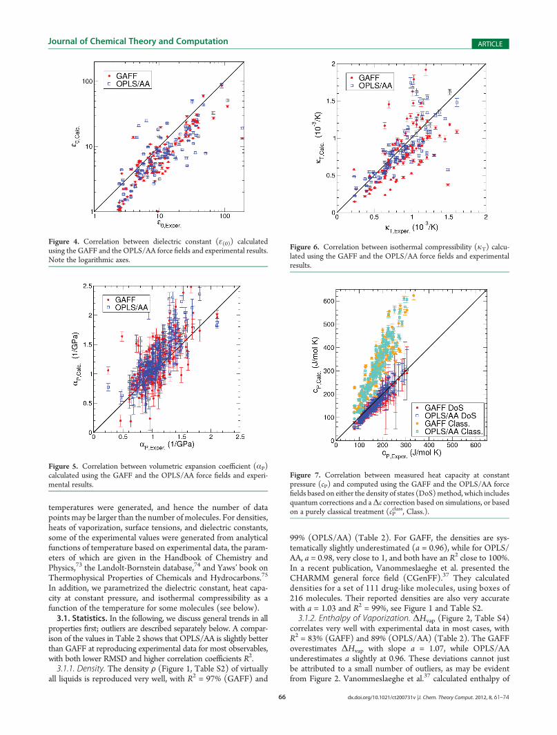
99% (OPLS/AA) (Table 2). For GAFF, the densities are sys-tematically slightly underestimated (a = 0.96), while for OPLS/AA, a = 0.98, very close to 1, and both have an R2 close to 100%.In a recent publication, Vanommeslaeghe et al. presented theCHARMM general force field (CGenFF).37 They calculateddensities for a set of 111 drug-like molecules, using boxes of216 molecules. Their reported densities are also very accuratewith a = 1.03 and R2 = 99%, see Figure 1 and Table S2.3.1.2. Enthalpy of Vaporization. ΔHvap (Figure 2, Table S4)

correlates very well with experimental data in most cases, withR2 = 83% (GAFF) and 89% (OPLS/AA) (Table 2). The GAFFoverestimates ΔHvap with slope a = 1.07, while OPLS/AAunderestimates a slightly at 0.96. These deviations cannot justbe attributed to a small number of outliers, as may be evidentfrom Figure 2. Vanommeslaeghe et al.37 calculated enthalpy of

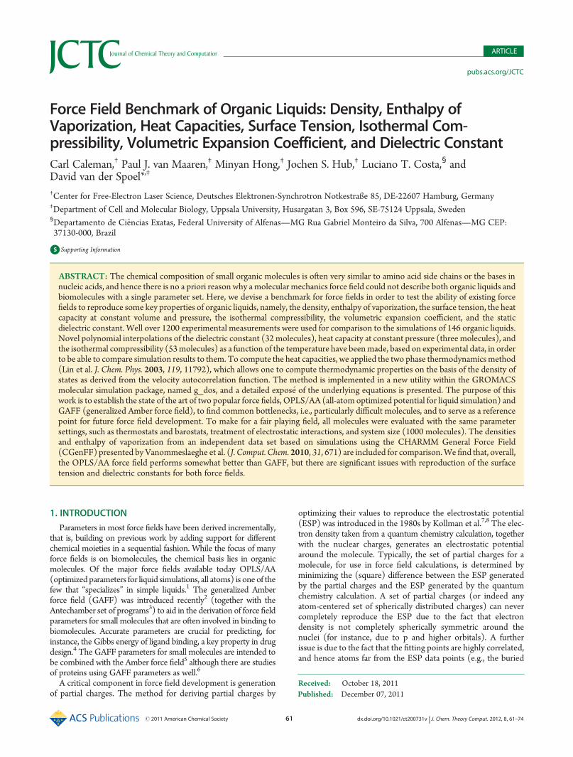
Figure 4. Correlation between dielectric constant (ε(0)) calculatedusing the GAFF and the OPLS/AA force fields and experimental results.Note the logarithmic axes.

Figure 5. Correlation between volumetric expansion coefficient (αP)calculated using the GAFF and the OPLS/AA force fields and experi-mental results.

Figure 6. Correlation between isothermal compressibility (kT) calcu-lated using the GAFF and the OPLS/AA force fields and experimentalresults.

Figure 7. Correlation between measured heat capacity at constantpressure (cP) and computed using the GAFF and the OPLS/AA forcefields based on either the density of states (DoS)method, which includesquantum corrections and aΔc correction based on simulations, or basedon a purely classical treatment (cP

class, Class.).



vaporization for a set of 95 small molecules. Like for OPLS/AA,ΔHvap is underestimated in CGenFF calculations with a slope ofa = 0.94. The correlation between experiments and simulation issimilar to the two force fields studied here, R2 = 84%. TheCGenFF data set is based on a comparable but different set ofmolecules than what has been analyzed here (37 molecules over-lap between the two studies). To simplify a comparison betweenOPLS/AA, GAFF, and CGenFF, we have listed the CGenFFΔHvap values from the study by Vanommeslaeghe et al. next toOPLS/AA and GAFF values in Table S3, and we have plottedthem in Figure 2.3.1.3. Surface Tension. The surface tension γ (Figure 3, Table

S4) seems to be underestimated systematically in both forcefields with slope a = 0.75 (GAFF) and 0.97 (OPLS/AA, Table 2).The interactions between molecules on the surface are notsufficiently strong, a well know problem with nonpolarizableforce fields.21,25,76 The values are spread around the diagonal forboth GAFF (R2 = 70%) and OPLS/AA (R2 = 89%), and hereagain OPLS/AA performs slightly better than GAFF.3.1.4. Dielectric Constant. For 32 molecules, a novel param-

etrization of the temperature dependence of the dielectric constantwas made on the basis of experimental values predominantly fromthe Landolt-Bornstein database.77 The parametrization is to a poly-nomial of second or third order (as is used in the Handbook ofChemistry and Physics73), and the resulting coefficients are given inTable 3. Interpolations of these polynomials were used in order tocompare the simulations to experimental data, and the fits arepresented in Figure S3 of the Supporting Information.The dielectric constant ε(0) (Figure 4, Table S5) appears to be

the most difficult property to reproduce in our simulations, withslopes a < 0.5 and R2e 60% for both force fields (Table 2). Apartfrom lacking explicit polarization, limited sampling (1000 molec-ules for 10 ns were used in all cases) may be one of the causes;another contributing factor is the high viscosity of molecules con-taining alcohol or amine groups, further aggravated by the factthat some of these molecules were simulated at temperaturesclose to the melting temperature.Some liquids have extremely large dielectric constants, e.g.,

methanamide (ε(0) = 109) andN-methylformamide (ε(0) = 190).

For these molecules, GAFF predicts 41 and 14, respectively, whileOPLS/AA predicts 51 and 19. Xie et al. report a simulateddielectric constant of 200 for N-methylformamide, using a polar-izable model, with only 256 molecules and 1 ns of simulation, butthe authors state that “The dielectric constants have only beenaveraged for 1 ns of simulation time, and they are almost certainnot yet converged.” Indeed, Whitfield et al. had previouslyconcluded that very long times (50 ns) may be needed to obtainconverged dielectric constants of molecules like N-methylaceta-mide because they tend to form long linear chains.78 Such chainscan in periodic simulation systems become “infinite”, which maycontribute to the long relaxation time. It should be noted, however,that formostmolecules in our study, the values are well converged,as witnessed by small error bars. Deviations from experimentalresults are therefore due predominantly to a lack of polarization andtoo low mobility of molecules. Interestingly, GAFF is somewhatbetter at predicting ε(0) than OPLS/AA (Table 2), most likelybecause the partial charges are somewhat higher for most molecules.3.1.5. Volumetric Expansion Coefficient. The volumetric ex-

pansion coefficient αP is plotted in Figure 5 and tabulated inTable S6. The slope of the correlation plots is slightly less than1 for both GAFF (a = 0.9) and OPLS/AA (a = 0.91), and there isa large spread around the y= x line for bothOPLS/AA andGAFFwith a RMSD of 0.3/GPa in both cases.3.1.6. Isothermal Compressibility. For 53 molecules, an inter-

polation of experimental values of the isothermal compressibilitykT as a function of the temperature was performed (Table 4 andFigure S3). The simulated kT’s are plotted versus the experi-mental values in Figure 6 and tabulated in Table S8. Like for αP,the spread in numbers is large, and the slope of the correlationplots is significantly less than 1 (GAFF, 0.66; OPLS/AA, 0.76,Table 2). In general, it seems that fluctuation properties are moredifficult to predict than simple linear averages. Although weapplied a very strict convergence criterion for the total energy of0.5 J/mol/ns per degree of freedom, it may be that even longerequilibration times and production simulations are needed.3.1.7. Heat Capacities. For three molecules, an interpolation

of experimental numbers is presented in Table 5 and Figure S4.The heat capacity is a difficult property to calculate due tosignificant quantum effects. The simple eq 7 produces numbers(cPclass) that are twice too high (Table 2). Since the energy taken

up by vibrations in a classical harmonic oscillator is much higherthan for a quantum harmonic oscillator at the same fre-quency, the cP

class values are too high. Introducing quantum cor-rections, in the manner proposed by Berens et al.,71 on whichthe two phase thermodynamics (2PT) method68�70 is based,presupposes that the frequencies in the classical simulation arecorrect: this is often the case since most force constants havebeen derived from spectroscopic experiments. It should be notedthat there is no a priori reason to assume that the intermoleculardegrees of freedom behave harmonically, as they are determinedby Coulomb and van der Waals interactions. Despite thesetheoretical shortcomings, the 2PT method produces reasonableresults for cP (see Figure 7, Table 2, and Table S8)—much closerto experiment than cP

class on any account. In order to compute cP,it is necessary to add a correctionΔc (eq 12) to the heat capacityat constant volume cV that is produced by the density of statesanalysis.Δc is underestimated by classical force field calculations;however, cP still is estimated reasonably, with a = 1.08 for GAFFand a = 1.02 for OPLS/AA with correlation coefficients R2 = 98%and 97%, respectively. If we compare just cV from our simulations(i.e., without adding in Δc) and subtract the experimental

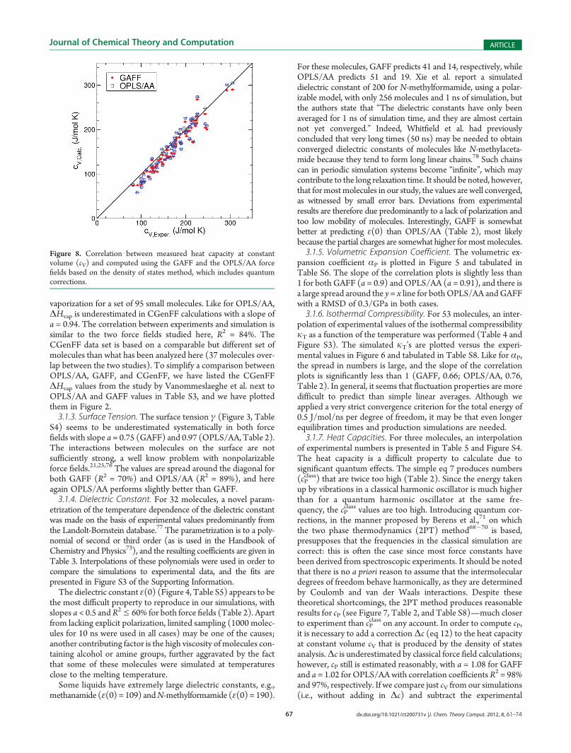
Figure 8. Correlation between measured heat capacity at constantvolume (cV) and computed using the GAFF and the OPLS/AA forcefields based on the density of states method, which includes quantumcorrections.



Δc from themeasured cP, we find a very good correlation (GAFF,a = 1.02, R2 = 97%; OPLS/AA, a = 1.04, R2 = 95%), see Figure 8and Table 2. Although correlation between experimental resultsand calculations can by no means validate the underlyingtheoretical model, it nevertheless indicates that the results aremeaningful, because we have approximately 70 experimental cVvalues to which to compare. Indeed, although the root-mean-square deviation (RMSD) from experimental results is similar forcV and cP, the fit to experimental results is much better (slope aclose to 1) for both OPLS/AA and GAFF. The DOS simulationswere performedwithout constraints, and the heat capacities dependdirectly on the intra- and intermolecular vibrations. Deviationsfrom the experimental heat capacities could therefore indicateproblems with the force constants for intramolecular motions.3.2. Outliers Per Force Field. Table 6 shows how the molec-

ular models of the individual molecules perform relative to theforce field as a whole. The average relative deviations in σ andaveraged over 1�8 data points (depending on the availability ofexperimental data) signals how well the force field performs foreach molecule. The properties used were density, enthalpy of

vaporization, surface tension, dielectric constant, volumetric ex-pansion coefficient, isothermal compressibility, and the heat capa-city at constant volume.Some types of molecules are problematic in both of the force

fields considered here. Small molecules containing more thanone Cl or Br atom generally have both density and enthalpy ofvaporization values that deviate significantly from experimentalreference. This is not the case for molecules containing only oneof these atoms, or molecules where there is a spacer (e.g., a CH2

group) between them. It could therefore be that the differencesare caused by overlapping atoms. By introducing a new atom type ofBr and Cl for the case where there are two such atoms next to eachother on the carbon chain, these problems might be resolved.The density and enthalpy of vaporization of methanoic acid

(formic acid) were particularly hard to reproduce, as was notedpreviously by Jedlovsky and Turi, who constructed a specificpotential for this molecule.79 The main feature responsible forthe improved model in this case was a higher charge (≈ 0.1e) onthe C�H atom than is used in either OPLS/AA (0) or GAFF(0.04). Methanoic acid forms very strong linear chains, which are

Table 3. Parameterization of Temperature Dependence of Dielectric Constants in a Polynomial Form ε(0) =A +BT +CT2 +DT3,Which Is the Same Form Used in the Handbook of Chemistry and Physics73a

molecule N χ2 Tmin Tmax A B C D

bromomethane 12 0.7 194.60 275.70 52.59 �2.812e�01 4.565e�04 0

methanol 92 1.0 175.62 337.75 226.69 �1.319e+00 2.937e�03 �2.359e�06

1,1,1,2,2-pentachloroethane 9 0.0 245.15 338.15 13.81 �5.527e�02 7.186e�05 0

1,1,2,2-tetrachloroethane 14 0.2 231.15 318.15 71.61 �3.630e�01 5.010e�04 0

1,2-dibromoethane 39 0.1 288.15 353.15 10.31 �3.114e�02 4.200e�05 0

1,1-dichloroethane 8 0.2 288.15 323.15 36.77 �1.300e�01 1.361e�04 0

2-chloroethanol 30 3.1 263.15 401.75 105.36 �3.245e�01 3.619e�05 5.019e�07

ethanamide 7 0.3 358.15 448.20 �200.55 1.551e+00 �2.239e�03 0

methyldisulfanylmethane 6 0.0 293.15 323.15 53.55 �2.539e�01 3.571e�04 0

2-aminoethanol 7 0.4 283.65 298.15 166.68 �7.576e�01 1.018e�03 0

1,3-dioxolan-2-one 24 0.5 309.46 364.15 223.34 �4.560e�01 9.143e�05 0

1,3-dioxolane 31 0.2 175.93 303.15 40.61 �2.507e�01 6.323e�04 �5.695e�07

dimethoxymethane 5 0.0 170.65 298.15 2.59 �9.298e�04 3.847e�06 0

ethylsulfanylethane 6 0.1 293.15 323.15 11.68 �1.994e�02 0.000e+00 0

2-methylpropan-2-amine 4 0.0 291.15 303.15 294.70 �1.887e+00 3.060e�03 0

thiophene 14 0.1 252.65 333.15 2.32 5.071e�03 �1.232e�05 0

furan 31 0.2 198.15 303.15 6.69 �2.044e�02 2.644e�05 0

pentane-2,4-dione 9 2.0 291.15 323.15 �532.57 3.658e+00 �5.982e�03 0

3-methylpyridine 6 1.0 293.15 333.00 35.54 �9.303e�02 4.307e�05 0

benzenethiol 6 0.3 293.15 358.15 5.72 �7.033e�03 7.362e�06 0

(E)-hex-2-ene 6 0.0 157.00 295.00 2.43 �1.132e�03 �1.372e�06 0

1-methoxy-2-(2-methoxyethoxy)ethane 5 0.0 298.15 333.15 32.07 �1.359e�01 1.766e�04 0

diethyl propanedioate 7 0.2 293.15 343.15 19.98 �5.034e�02 3.345e�05 0

2,4,6-trimethylpyridine 10 0.1 293.15 358.15 16.67 �3.036e�02 2.361e�06 0

triethyl phosphate 6 0.1 294.15 333.15 �1.59 1.317e�01 �2.780e�04 0

phenylmethanol 26 0.2 278.15 363.15 105.48 �5.130e�01 6.802e�04 0

tetrahydrothiophene 1,1-dioxide 57 0.4 300.75 398.15 488.81 �3.732e+00 1.055e�02 �1.017e�05

2,4,6-trimethylpyridine 10 0.1 293.15 358.15 16.67 �3.036e�02 2.361e�06 0

dimethoxymethane 5 0.0 170.65 298.15 2.92 �4.106e�03 1.126e�05 0

1,3-dichloropropane 5 0.1 298.15 333.15 �61.39 4.818e�01 �8.107e�04 0

methylsulfanylmethane 6 0.2 273.30 310.48 23.41 �8.896e�02 1.076e�04 0

1,2-ethanedithiol 3 0.0 293.15 333.15 11.23 �1.350e�02 0.000e+00 0a Tmin and Tmax (K) indicate the validity range of the parameterization. N indicates the number of points in the fit; χ2 is the root mean square deviation.See the Supporting Information for details.



Table 4. Parameterization ofTemperatureDependence of IsothermalCompressibilityConstants in a Polynomial FormjT=A+BT+CT2a

molecule N χ2 Tmin Tmax A B C

dichloromethane 3 0.000 293.15 303.15 �1.709e+01 1.144e�01 �1.800e�04

methanamide 5 0.008 288.15 323.15 1.352e�01 9.161e�04 0

nitromethane 4 0.020 298.15 323.15 �1.253e+00 6.666e�03 0

methanol 24 0.014 213.15 333.15 1.004e+00 �6.791e�03 2.557e�05

acetonitrile 5 0.000 298.15 318.15 3.174e+00 �2.209e�02 5.114e�05

1,1,2,2-tetrachloroethane 2 0.000 293.15 303.15 �4.962e�01 3.900e�03 0

1,1,2-trichloroethane 7 0.002 288.15 318.15 �7.213e�01 4.937e�03 0

bromoethane 5 0.010 273.15 323.15 9.748e+00 �6.685e�02 1.287e�04

N-methylformamide 4 0.011 288.15 313.15 6.378e�03 1.968e�03 0

nitroethane 3 0.015 298.15 323.15 �9.873e�01 6.004e�03 0

ethanol 16 0.007 203.15 363.15 1.280e+00 �8.946e�03 2.857e�05

methylsulfinylmethane 7 0.030 293.15 353.15 5.206e�01 �3.136e�03 1.052e�05

2-aminoethanol 6 0.000 278.15 333.15 7.273e�01 �4.276e�03 1.051e�05

1,3-dichloropropane 6 0.000 283.15 323.15 6.932e�01 �4.785e�03 1.678e�05

propan-2-one 10 0.010 293.15 328.15 �3.053e+00 1.468e�02 0

methyl acetate 8 0.012 293.15 328.15 �2.562e+00 1.249e�02 0

1,3-dioxolane 2 0.000 293.15 313.15 �1.317e+00 6.960e�03 0

1-bromopropane 7 0.003 288.15 318.15 �1.264e+00 8.037e�03 0

N,N-dimethylformamide 18 0.018 288.15 333.20 1.748e+00 �1.073e�02 2.367e�05

1-nitropropane 3 0.004 298.15 323.15 �1.111e+00 6.420e�03 0

2-nitropropane 3 0.020 298.15 323.15 �1.060e+00 6.604e�03 0

1,4-dichlorobutane 5 0.004 288.15 318.15 �8.725e�01 5.246e�03 0

propane-1,2,3-triol 19 0.003 293.15 473.15 8.358e�01 �4.323e�03 7.862e�06

propan-1-amine 6 0.036 293.15 323.15 �2.469e+00 1.238e�02 0

N,N-dimethylacetamide 5 0.015 288.15 318.15 �5.890e�01 4.142e�03 0

butan-1-ol 15 0.021 293.15 393.15 1.307e+00 �8.833e�03 2.543e�05

N-ethylethanamine 5 0.002 298.15 318.15 7.548e+00 �5.536e�02 1.188e�04

butan-1-amine 8 0.003 298.15 328.15 2.330e+00 �1.702e�02 4.371e�05

ethyl acetate 9 0.012 298.15 350.30 5.084e+00 �3.567e�02 7.598e�05

oxolane 5 0.001 278.15 323.15 �9.434e�01 4.999e�03 4.886e�06

1-bromobutane 12 0.000 298.15 333.15 2.650e+00 �1.860e�02 4.413e�05

1-chlorobutane 10 0.029 293.15 318.15 �2.399e+00 1.205e�02 0

pentanenitrile 5 0.005 283.15 323.15 8.811e�01 �7.004e�03 2.429e�05

ethyl propanoate 15 0.022 278.15 338.15 6.964e�01 �7.128e�03 2.882e�05

2-methylbutan-2-ol 2 0.000 293.15 298.15 �1.495e+00 8.600e�03 0

pentan-1-ol 8 0.010 293.15 333.15 3.158e+00 �2.044e�02 4.292e�05

pentan-3-ol 10 0.003 293.15 368.15 4.952e+00 �3.315e�02 6.587e�05

nitrobenzene 5 0.009 298.15 323.15 �3.337e�01 2.832e�03 0

cyclohexanone 5 0.021 298.15 308.15 �9.399e�01 5.421e�03 0

hexan-2-one 8 0.022 278.15 338.15 �1.451e+00 8.315e�03 0

1-methoxy-2-(2-methoxyethoxy)ethane 6 0.001 298.15 318.15 �8.794e�01 5.105e�03 0

N,N-diethylethanamine 8 0.006 298.15 328.15 4.400e+00 �3.405e�02 8.064e�05

N-propan-2-ylpropan-2-amine 7 0.001 298.15 328.15 9.459e+00 �6.732e�02 1.357e�04

methoxybenzene 5 0.043 298.15 338.15 �1.520e+00 7.287e�03 0

3-methylphenol 6 0.041 298.15 413.15 1.744e+00 �1.029e�02 2.104e�05

toluene 50 0.006 288.15 333.15 2.342e+00 �1.627e�02 3.853e�05

diethyl propanedioate 7 0.000 298.15 328.15 2.164e+00 �1.397e�02 3.048e�05

heptan-2-one 2 0.000 293.15 298.15 �8.915e�01 6.200e�03 0

ethylbenzene 7 0.008 293.15 333.15 2.524e+00 �1.652e�02 3.683e�05

1,2-dimethylbenzene 10 0.022 273.15 417.50 �2.914e�01 1.846e�03 6.429e�06

octan-1-ol 16 0.033 293.15 413.15 2.242e+00 �1.449e�02 3.206e�05

quinoline 2 0.000 333.15 373.15 �5.477e�01 3.320e�03 0

(1-methylethyl)benzene 3 0.003 293.15 298.15 �6.340e�01 5.110e�03 0

a Tmin and Tmax (K) indicate the validity range of the parameterization. N indicates the number of points in the fit; χ2 is the root mean square deviation.See the Supporting Information for details.



difficult to break. This leads to long correlation times for thesystem dipoles and to dielectric constants that are far from theexperimental values (Table S5).Benzaldehyde and furan are also problematic in both force

fields. Even if they both generate decent densities and enthalpiesof vaporization, the other properties (surface tension, dielectricconstant, and thermal expansion coefficient) are far from theexperimental values.Molecules containing a nitro group (specially nitromethane,

1-nitropropane, and 2-nitropropane) stick out as a problematicgroup in GAFF. The charges on nitro groups are high, leading tohigh density and enthalpy of vaporization.The standard OPLS/AA parametrization of alcohols has been

reported to perform poorly for octan-1-ol. MacCallum andTieleman80 therefore derived a specific united atom potentialof the molecule where they used modified charges on theheadgroup. The OPLS/AA parametrization investigated heregives both too high a density and too high an enthalpy of vapo-rization, and therefore the other properties investigated for thismolecules also deviate from experimental results. Methyl-2-methylprop-2-enaote shows similar problems, and this couldprobably be corrected in a similar way. It should be noted that,compared to GAFF, the charges on the headgroup in these twomolecules are relatively high in OPLS/AA.

4. DISCUSSION

The development of force fields for molecular simulation iscritically dependent on the availability of good reference data,preferably from experimental sources. All force fields, be theyempirical, purely derived from quantum-mechanics, or a combi-nation of the two, will eventually have to face the test of com-paring predicted to measured values. There is a large amount ofliterature on force field testing for proteins and peptides,57,81�87

nucleic acids,88�91 carbohydrates,92 specific organic molecules orprotein fragments,20,26,93�97 and ions,98�101 to list but a few. Inaddition, there are indirect force field tests, for instance of thebinding energy in protein�ligand complexes,16,102 protein struc-ture prediction,103 or of force-field-based docking codes.104�106

It is interesting to mention the industrial fluid propertiessimulation challenges, which are stimulating modelers to predictproperties of liquids by any means, including molecular simula-tion.107,108

Here, we have introduced a benchmark set of 146 liquids inorder to assess two popular all atom force fields, OPLS/AA andGAFF, and to set a standard for future force fields. For com-parison, we have included an independent density and enthalpyof vaporization data set computed using CGenFF, based ona similar set of molecules.37 Calculated density, enthalpy ofvaporization, heat capacities, surface tension, dielectric constants,

Table 5. Parameterization of Temperature Dependence ofHeat Capacity at Constant Pressure in a Polynomial FormcP = A + BTa

molecule N χ2 Tmin Tmax A B

1,3-dioxolane 9 0.187 288.15 328.15 4.371e+01 2.613e�01

1,2,3,4-tetrafluorobenzene 41 0.145 235.47 319.79 1.158e+02 2.491e�01

1,2,3,5-tetrafluorobenzene 25 0.343 229.32 311.18 1.186e+02 2.400e�01a Tmin and Tmax (K) indicate the validity range of the parameterization.N indicates the number of points in the fit; χ2 is the root mean squaredeviation. See the Supporting Information for details.

Table 6. Average Relative Deviation (σ) from ExperimentalValues, in Brackets, the Number of Observablesa

name CGenFF GAFF OPLS/AA

1. chloroform 2.1(6) 3.0(7)

2. dichloro(fluoro)methane 1.0(4) 1.3(4)

3. dibromomethane 2.9(6) 1.7(7)

4. dichloromethane 1.7(7) 3.6(7)

5. methanal 0.3(4) 0.3(4)

6. methanoic acid 4.5(6) 2.6(7)

7. bromomethane 1.4(3) 0.4(3)

8. methanamide 0.0(1) 1.2(7) 0.4(6)

9. nitromethane 2.0(7) 0.8(7)

10. methanol 0.0(2) 0.8(7) 0.8(7)

11. 1,1,1,2,2-pentachloroethane 0.5(4) 0.8(4)

12. 1,1,2,2-tetrachloroethane 1.7(7) 1.7(7)

13. 1,1-dichloroethene 1.7(4) 0.8(4)

14. 1,1,2-trichloroethane 1.2(7) 0.9(7)

15. acetonitrile 0.0(1) 1.1(7) 2.2(7)

16. 1,2-dibromoethane 2.6(7) 4.0(7)

17. 1,1-dichloroethane 0.0(1) 0.7(7) 1.7(7)

18. 1,2-dichloroethane 1.6(7) 1.2(7)

19. methyl formate 0.9(4) 0.8(5)

20. bromoethane 0.0(1) 2.2(7) 0.6(7)

21. chloroethane 0.0(1) 0.8(5) 1.3(5)

22. 2-chloroethanol 0.4(4) 0.5(4)

23. ethanamide 0.2(4) 0.8(5)

24. N-methylformamide 1.4(7) 1.4(7)

25. nitroethane 1.5(7) 0.7(7)

26. methoxymethane 0.5(5) 1.3(5)

27. ethanol 0.0(2) 1.0(7) 0.7(6)

28. 1,2-ethanedithiol 0.6(3) 0.1(3)

29. methyldisulfanylmethane 0.1(2) 1.2(5) 1.6(5)

30. methylsulfinylmethane 0.1(1) 1.0(7) 0.6(7)

31. methylsulfanylmethane 1.4(5) 1.2(5)

32. 2-aminoethanol 1.2(5) 1.3(6)

33. ethane-1,2-diamine 1.2(7) 1.9(7)

34. prop-2-enenitrile 1.0(5) 1.2(5)

35. 1,3-dioxolan-2-one 0.5(5) 0.2(4)

36. propanenitrile 1.1(7) 1.9(7)

37. 1,2-dibromopropane 1.1(5) 0.6(4)

38. 1,3-dichloropropane 0.9(7) 1.0(7)

39. (2R)-2-methyloxirane 0.0(2) 0.1(2)

40. propan-2-one 0.0(2) 1.0(7) 0.7(7)

41. methyl acetate 0.0(2) 1.3(7) 0.9(7)

42. 1,3-dioxolane 0.0(1) 1.2(4) 0.6(4)

43. 2-iodopropane 0.7(5) 1.1(5)

44. 1-bromopropane 1.3(7) 0.6(7)

45. N,N-dimethylformamide 0.7(6) 0.5(6)

46. N-methylacetamide 0.0(1) 0.4(4) 0.2(4)

47. 1-nitropropane 1.6(7) 1.2(7)

48. 2-nitropropane 1.6(7) 0.9(7)

49. dimethoxymethane 0.8(5) 0.9(5)

50. propane-1,2,3-triol 1.3(6) 0.8(6)

51. propan-1-amine 1.1(7) 1.5(7)

52. propan-2-amine 0.7(5) 0.6(4)

53. 2-methylpropane 0.0(1) 0.8(5) 1.1(5)



volumetric expansion coefficients, and isothermal compressibil-ity from the two force fields are compared to experimental values.Indeed the benchmark is quite revealing, in that systematicdeviations can be found and rationalized. The knowledge aboutsuch deviations will hopefully be useful for further developmentof the force fields.

To a first approximation, molecular vibrations can be de-scribed as quantum harmonic oscillators.109 Classical harmonicoscillators do not describe the properties of quantum harmonicoscillators, which makes it necessary to implement corrections incomputing for instance heat capacities. The two phase thermo-dynamics method employed here for estimating cP and cV relieson the force constants of the force field used, and on the effectivefrequencies in the simulations. The density of states obtained

Table 6. Continuedname CGenFF GAFF OPLS/AA

54. ethylsulfanylethane 0.6(5) 0.7(5)

55. butane-1-thiol 0.9(5) 0.5(5)

56. butan-1-ol 1.1(7) 0.9(7)

57. 2-methylpropan-2-ol 0.4(2) 0.1(2)

58. butane-1,4-diol 0.9(6) 0.4(6)

59. (2-hydroxyethoxy)ethan-2-ol 1.2(4) 1.1(5)

60. N-ethylethanamine 1.1(7) 1.2(7)

61. butan-1-amine 1.1(7) 0.9(7)

62. 2-methylpropan-2-amine 1.0(5) 0.8(5)

63. 2-(2-hydroxyethylamino)ethanol 0.5(4) 0.4(4)

64. pyrimidine 0.0(2) 0.7(4) 0.6(4)

65. furan 0.2(2) 1.9(5) 1.9(5)

66. thiophene 0.0(2) 0.7(4) 0.3(5)

67. 1H-pyrrole 0.1(1) 1.3(7) 1.1(7)

68. ethenyl acetate 0.5(4) 0.8(4)

69. oxolan-2-one 0.3(3) 0.3(4)

70. acetyl acetate 1.2(4) 1.2(4)

71. 1,4-dichlorobutane 0.6(7) 0.8(7)

72. oxolane 0.6(6) 1.3(7)

73. ethoxyethene 0.3(3) 0.2(3)

74. ethyl acetate 0.0(2) 1.2(7) 1.1(7)

75. tetrahydrothiophene 1,1-dioxide 0.8(4) 0.9(4)

76. thiolane 0.5(4) 0.4(4)

77. 1-bromobutane 1.1(7) 0.7(7)

78. 1-chlorobutane 1.4(7) 1.8(7)

79. pyrrolidine 0.1(1) 1.3(7) 1.3(7)

80. N,N-dimethylacetamide 1.0(7) 0.9(7)

81. morpholine 0.8(5) 0.9(5)

82. pyridine 0.1(2) 0.6(6) 0.9(7)

83. cyclopentanone 0.8(5) 0.6(5)

84. 1-cyclopropylethanone 0.2(2) 0.1(2)

85. pentane-2,4-dione 0.9(5) 1.3(5)

86. methyl 2-methylprop-2-enoate 0.8(5) 3.6(5)

87. pentanenitrile 0.6(6) 1.6(7)

88. ethyl propanoate 1.3(7) 1.1(7)

89. diethyl carbonate 2.1(7) 0.7(6)

90. pentan-1-ol 1.0(7) 0.9(7)

91. pentan-3-ol 1.0(7) 1.1(7)

92. 2-methylbutan-2-ol 1.1(5) 0.5(5)

93. pentane-1,5-diol 0.8(6) 0.6(6)

94. pentan-3-amine 0.5(4) 0.6(4)

95. 1,2,3,4-tetrafluorobenzene 0.2(2) 0.1(2)

96. 1,2,3,5-tetrafluorobenzene 0.2(2) 0.1(2)

97. 1,3-difluorobenzene 0.2(2) 0.7(4) 1.3(5)

98. 1,2-difluorobenzene 0.7(4) 1.0(5)

99. fluorobenzene 0.1(2) 1.6(7) 0.5(6)

100. nitrobenzene 0.0(2) 1.1(7) 1.1(7)

101. 2-chloroaniline 0.9(4) 0.6(4)

102. phenol 0.8(4) 0.9(5)

103. benzenethiol 1.4(5) 1.3(5)

104. 2-methylpyridine 0.3(4) 0.9(5)

105. 3-methylpyridine 0.1(2) 0.8(5) 0.6(5)

106. 4-methylpyridine 0.0(2) 1.1(7) 0.4(6)

107. cyclohexanone 1.0(7) 0.9(7)

108. (E)-hex-2-ene 0.0(2) 0.0(2) 0.0(2)

Table 6. Continuedname CGenFF GAFF OPLS/AA

109. hexan-2-one 0.8(6) 0.9(7)

110. 2,4,6-trimethyl-1,3,5-trioxane 1.6(4) 1.0(4)

111. cyclohexanamine 0.8(5) 0.7(5)

112. 2-propan-2-yloxypropane 3.3(7) 0.9(7)

113. 1-methoxy-2-(2-methoxyethoxy)ethane 1.5(7) 1.1(7)

114. triethyl phosphate 2.8(6) 2.2(6)

115. N,N-diethylethanamine 1.2(7) 1.0(7)

116. N-propan-2-ylpropan-2-amine 0.8(6) 0.6(6)

117. trifluoromethylbenzene 0.8(5) 0.5(4)

118. benzonitrile 1.0(5) 1.0(5)

119. benzaldehyde 0.2(2) 5.7(7) 3.7(6)

120. toluene 0.1(2) 1.6(7) 1.3(7)

121. methoxybenzene 0.1(2) 1.2(7) 1.1(7)

122. phenylmethanol 1.0(5) 0.8(5)

123. 2-methylphenol 0.9(5) 0.8(5)

124. 3-methylphenol 1.0(5) 0.9(5)

125. 4-methylphenol 0.1(1) 1.2(5) 0.7(5)

126. diethyl propanedioate 1.1(4) 0.8(4)

127. 2,4-dimethylpentan-3-one 0.6(4) 0.4(4)

128. heptan-2-one 1.1(7) 0.7(7)

129. ethenylbenzene 1.2(5) 1.1(5)

130. 1-phenylethanone 1.0(7) 1.1(7)

131. methyl benzoate 0.9(7) 1.0(7)

132. methyl 2-hydroxybenzoate 1.1(5) 0.4(4)

133. ethylbenzene 0.1(2) 1.4(7) 1.1(7)

134. 1,2-dimethylbenzene 0.1(1) 1.7(7) 1.0(7)

135. 1,2-dimethoxybenzene 0.4(4) 0.6(5)

136. 2,4,6-trimethylpyridine 0.9(5) 1.0(5)

137. octan-1-ol 0.8(6) 1.7(7)

138. 1-butoxybutane 0.7(4) 1.0(5)

139. N-butylbutan-1-amine 0.9(7) 0.8(7)

140. isoquinoline 0.0(1) 0.7(4) 1.3(4)

141. quinoline 0.1(2) 1.1(7) 1.2(7)

142. (1-methylethyl)benzene 0.1(2) 1.0(6) 0.7(6)

143. 1,2,4-trimethylbenzene 0.1(1) 1.2(6) 1.0(6)

144. 2,6-dimethylheptan-4-one 1.0(5) 0.9(5)

145. 1-chloronaphthalene 0.5(6) 1.3(7)

146. phenoxybenzene 0.6(4) 1.1(5)aAverage relative deviation larger than 1σ is printed in bold, larger than1.5σ in bold italic.



from the velocity autocorrelation is convoluted by a weightingfunction derived from the partition function for a quantumharmonic oscillator in order to obtain a heat capacity for acorresponding quantum liquid. If a force field would allow one todirectly reproduce the “correct” density of states, one could usethe much simpler fluctuation formulas, as described by Allen andTildesley;38 however, heat capacities computed in this manneroverestimate the experimental values by about 100% for OPLS/AA and GAFF (Table S10). Going beyond the harmonic ap-proximation should therefore be considered by force fielddevelopers. Despite efforts in the context of the MMF94 forcefield110 and the MM3-MM4 family of force fields,111�113 this hasnot been widely adopted in the biomolecular simulation com-munity, although the polarizable AMOEBA force field114 doesfeature anharmonic bond and angle potentials as well. In prin-ciple, it should be advantageous to use for instance Car�Parrinellomolecular dynamics,115 in order to more faithfully represent aliquid than is possible in a classical simulation. This was attemp-ted by Kuo et al. for water.116 They find a large scatter in cP valuesdue to limited sampling, but also a systematic deviation from theexperimental value. Obviously, the computational bottleneckthat would be introduced by CPMD or related methods willremain difficult to surmount for the immediate future, and there-fore force-field-based methods remain necessary. Nevertheless, itis encouraging that there is a trend to use molecular dynamicssimulations based on density functional theory codes to studyvibrational properties of biomolecular systems beyond the har-monic approximation.117�119

The dielectric constant seems to be the hardest nut to crack.Nonpolarizable force fields (such as GAFF and OPLS/AA) areknown to have difficulties in reproducing the dielectric constantand to some extent also the surface tension. In the case of water,for which a large number of force fields have been developed,there are several studies that describe this (for a review, see, forexample, Guillot25). Improving the dielectric function oftenturns out to be done at the cost of the enthalpy of vaporizationand the free energy of solvation—properties that may be moreimportant to reproduce in biomolecular simulations. In additionto systematic problems, like sampling or the lack of polarizationin our simulations,120 the temperature dependence of the di-electric constant provides both a challenge and an opportunityfor future force field development. For most molecules, thetemperature dependence is very strong, because molecular mo-tion is the largest factor contributing to ε(0). In his review ofwater models, Guillot has pointed out that the relation betweendielectric constant and other properties is complex, and hence itcan be used to test and validate force fields, but not likely as atarget for force field optimization.25

The benchmark we present here allows one to pinpoint sys-tematic errors in force fields due to the fact that most chemicalmoieties are represented more than once. The overall perfor-mance of GAFF is surprisingly good, seeing that the parameterdevelopment was not aimed at liquids. The results from theOPLS/AA force field are slightly better than GAFF, obviouslydue to the fact that OPLS/AA was parametrized for liquids. TheCHARMM generalized force field seems to be even slightlybetter, at least for density and enthalpy of vaporization.37 It isreassuring for applications of force field calculations beyondliquids that the parameters in most cases are reasonable; how-ever, the results presented here also show that blind faith in forcefields is not warranted in all cases. In Table 2, we list the root-mean-square deviation, as well as the average relative deviation,

of the calculated values from the experimental, for each propertywe have analyzed. Even if our set of molecules is limited to 146,these numbers give a measurement of howwell the properties arereproduced in the two force fields, at least for molecules similar tothe set presented here.

Wang and Tingjun have recently reported a similar forcefield test of 71 organicmolecules based on theGAFFandOPLS/AAforce fields.32 They report densities and enthalpies of vaporiza-tion for these molecules and find small deviations from experi-mental results that are comparable to our numbers. It is encourag-ing to note that these authors were able to improve the corres-pondence to experimental numbers by tuning the Lennard-Jonesparameters of some of the atom types. How this affects the otherproperties that we have studied here, in particular, the dielectricconstant and the surface tension, remains to be determined, but itis likely that just tweaking the Lennard-Jones parameters is notsufficient to cure the significant and systematic deviations ob-served for those properties.

Mobley et al. have performed free energy of solvation (ΔGhyd)benchmarks, reporting a RMS error from experimental numbersof 5.2 kJ/mol for more than 500 molecules.121,122 This number iscomparable to the RMSD of 6.5 kJ/mol we computed forΔHvap

for OPLS/AA (10.6 kJ/mol for GAFF and 4.7 kJ/mol forCGenFF37). Since both numbers are to a large extent determinedby the intermolecular energies, we can conclude that the RMSerror in intermolecular energies for (“small”) organic moleculesis 5�6 kJ/mol using state of the art simulations and nonpolariz-able force fields. It should be noted that this result may be biasedby the choice of test set, as has been shown in the context of theSAMPL contest where hydration energies were to be predicted.123,124

It was found here that larger molecules with multiple functionalgroups have similar deviations from the experimental hydrationenergy—errors up to 10 kJ/mol.123 It seems plausible that part ofthis error is due to the simple nonpolarizable water model used,however, since the enthalpy of vaporization is approximatelyadditive (which can be seen by plottingΔHvap for, e.g., alkanes asa function of the number of carbons), the error per functionalgroup should still be relatively low, less than 5 kJ/mol for mostgroups. In the present work, we studied pure liquids only, pro-viding a simpler test set than what has been used in previousstudies. Further tests on pure liquids and liquid mixtures shouldprovide a more detailed understanding of the predictive power offorce field calculations. At the same time, systematic methods forforce field development23,125 could be used for the improvementof classical force fields.

’ASSOCIATED CONTENT

bS Supporting Information. Complete molecular topologiesand structures for use with the GROMACS software suite as wellas equilibrated liquid boxes containing coordinates for all 146systems are available from our Web site http://virtualchemistry.org . Simulation parameter files are available in a zip file. The PDFfile contains a derivation of the two phase thermodynamicsmethod, as well as four supporting figures and 13 tables. FigureS1 shows ΔD eq 4; Figure S2, the fits to experimental data as afunction of temperature for the dielectric constants; Figure S3,the fits to experimental data as a function of temperature for theheat capacity; and Figure S4, the fits to experimental data as afunction of temperature for the isothermal compressibility.Tables S11�S13 give the experimental references correspondingto Figures S2�S4 for eachmolecule. Table S1 contains a list of all



molecules with formula, molecular weight, CAS number, andChemSpider ID. Full lists of the calculated values for all proper-ties as well as experimental and CGenFF37 reference data (whereapplicable) are presented for liquid densities (Table S2), en-thalpy of vaporization (Table S3), surface tension (Table S4),dielectric constant (Table S5), volumetric expansion coefficients(Table S6), isothermal compressibility (Table S7), heat capacitycP (Table S8), heat capacity cV (Table S9), and heat capacity cP

class

(Table S10). The tables are presented using the Hill system.126

This information is available free of charge via the Internet athttp://pubs.acs.org.

’AUTHOR INFORMATION

Corresponding Author*E-mail: [email protected].

NotesThe authors declare no competing financial interest.

’ACKNOWLEDGMENT

The Swedish research council is acknowledged for somefinancial support to D.v.d.S. and for a grant of computer time(SNIC-022-09/10) through the national supercomputer center(NSC) in Link€oping and the parallel computing center (PDC) inStockholm, Sweden. C.C. acknowledges financial support fromthe Helmholtz Association through the Center for Free-ElectronLaser Science. This study was also supported by a Marie CurieIntra-European Fellowship within the seventh European Com-munity Framework Programme to J.S.H. We would like to thankG€oran Wallin for stimulating discussions and Marjolein van derSpoel for help with collecting experimental data.

’REFERENCES

(1) Jorgensen, W. L.; Tirado-Rives, J. Proc. Natl. Acad. Sci. U.S.A.2005, 102, 6665–6670.(2) Wang, J.; Wolf, R.M.; Caldwell, J. W.; Kollman, P. A.; Case, D. A.

J. Comput. Chem. 2004, 25, 1157–1174.(3) Wang, J.; Wang, W.; Kollman, P. A.; Case, D. A. J. Comput. Chem.

2005, 25, 1157–1174.(4) Hetenyi, C.; Paragi, G.; Maran, U.; Timar, Z.; Karelson, M.;

Penke, B. J. Am. Chem. Soc. 2006, 128, 1233–1239.(5) Case, D. A.; Cheatham, T. E., III; Darden, T.; Gohlke, H.; Luo,

R.; Merz, K. M., Jr.; Onufriev, A.; Simmerling, C.; Wang, B.; Woods, R. J.J. Comput. Chem. 2005, 26, 1668–1688.(6) Fujitani, H.; Tanida, Y.; Matsuura, A. Phys. Rev. E 2009, 79, 021914.(7) Singh, U. C.; Kollman, P. A. J. Comput. Chem. 1984, 5, 129–145.(8) Besler, B. H.; Merz, K. M., Jr.; Kollman, P. A. J. Comput. Chem.

1990, 11, 431–439.(9) Francl, M. M.; Carey, C.; Chirlian, L. E.; Gange, D. M. J. Comput.

Chem. 1996, 17, 367–383.(10) Francl, M. M.; Chirlian, L. E. Rev. Comput. Chem. 2000, 14, 1–31.(11) Bayly, C. I.; Cieplak, P.; Cornell, W. D.; Kollman, P. A. J. Phys.

Chem. 1993, 97, 10269–10280.(12) Jakalian, A.; Bush, B. L.; Jack, D. B.; Bayly, C. I. J. Comput. Chem.

2000, 21, 132–146.(13) Jakalian, A.; Jack, D. B.; Bayly, C. I. J. Comput. Chem. 2002,

23, 1623–1641.(14) Mobley, D. L.; Dumont, E.; Chodera, J. D.; Dill, K. A. J. Phys.

Chem. B 2007, 111, 2242–2254.(15) Mobley, D. L.; Dumont, E.; Chodera, J. D.; Dill, K. A. J. Phys.

Chem. B 2011, 115, 1329–1332.(16) Wallin, G.; Nervall, M.; Carlsson, J.; Åqvist, J. J. Chem. Theory

Comput. 2009, 5, 380–395.

(17) Storer, J. W.; Giesen, D. J.; Cramer, C. J.; Truhlar, D. G.J. Comput.-Aided Mol. Des. 1995, 9, 87–110.

(18) Kaminski,G.; Jorgensen,W. J. Phys. Chem.B.1998,102, 1787–1796.(19) Chandrasekhar, J.; Shariffskul, S.; Jorgensen, W. J. Phys. Chem.

B. 2002, 106, 8078–8085.(20) Shirts, M. R.; Pitera, J. W.; Swope, W. C.; Pande, V. S. J. Chem.

Phys. 2003, 119, 5740–5761.(21) Wensink, E. J. W.; Hoffmann, A. C.; van Maaren, P. J.; van der

Spoel, D. J. Chem. Phys. 2003, 119, 7308–7317.(22) van der Spoel, D.; van Maaren, P. J.; Larsson, P.; Timneanu, N.

J. Phys. Chem. B. 2006, 110, 4393–4398.(23) van der Spoel, D.; vanMaaren, P. J.; Berendsen, H. J. C. J. Chem.

Phys. 1998, 108, 10220–10230.(24) Mark, P.; Nilsson, L. J. Comput. Chem. 2002, 23, 1211–1219.(25) Guillot, B. J. Mol. Liq. 2002, 101, 219–260.(26) Hess, B.; van der Vegt, N. F. A. J. Phys. Chem. B 2006,

110, 17616–17626.(27) Caleman, C.; van der Spoel, D. J. Chem. Phys. 2006, 125, 154508.(28) Caleman, C.; van der Spoel, D. Phys. Chem. Chem. Phys. 2007,

9, 5105–5111.(29) Vega, C.; Abascal, J. L. F. Phys. Chem. Chem. Phys. 2011.(30) Kaminski, G.; Duffy, E. M.; Matsui, T.; Jorgensen, W. L. J. Phys.

Chem. 1994, 98, 13077–13082.(31) Kaminski, G.; Jorgensen, W. L. J. Phys. Chem. 1996, 100,

18010–18013.(32) Wang, J.; Tingjun, H. J. Chem. Theory Comput. 2011, 7, 2151–2165.(33) Berendsen, H. J. C.; van der Spoel, D.; van Drunen, R. Comput.

Phys. Commun. 1995, 91, 43–56.(34) Lindahl, E.; Hess, B.; van der Spoel, D. J. Mol. Model. 2001,

7, 306–317.(35) van der Spoel, D.; Lindahl, E.;Hess, B.; Groenhof, G.;Mark, A. E.;

Berendsen, H. J. C. J. Comput. Chem. 2005, 26, 1701–1718.(36) Hess, B.; Kutzner, C.; van der Spoel, D.; Lindahl, E. J. Chem.

Theory Comput. 2008, 4, 435–447.(37) Vanommeslaeghe, K.; Hatcher, E.; Acharya, C.; Kundu, S.;

Zhong, S.; Shim, J.; Darian, E.; Guvench, O.; Lopes, P.; Vorobyov, I.;Mackerell, A. D. J. Comput. Chem. 2010, 31, 671–690.

(38) Allen, M. P.; Tildesley, D. J. Computer Simulation of Liquids;Oxford Science Publications: Oxford, 1987.

(39) Jorgensen, W. L.; Maxwell, D. S.; Tirado-Rives, J. J. Am. Chem.Soc. 1996, 118, 11225–11236.

(40) Schuettelkopf, A.W.; van Aalten, D.M. F.Acta Crystallogr., Sect.D. 2004, 60, 1355–1363.

(41) Schaftenaar, G.; Noordik, J. H. J. Comput.-Aided Mol. Des. 2000,14, 123–134.

(42) Frisch, M. J.; et al. Gaussian 03, Revision C.02; Gaussian, Inc.:Wallingford, CT, 2004.

(43) Krishnan, R.; Binkley, J.; Seeger, R.; Pople, J. J. Chem. Phys.1980, 72, 650–654.

(44) McLean, A.; Chandler, G. J. Chem. Phys. 1980, 72, 5639–5648.(45) Glukhovtsev, M.; Pross, A.; McGrath, M.; Radom, L. J. Chem.

Phys. 1995, 103, 1878–1885.(46) Curtiss, L.; McGrath, M.; Blaudeau, J.; Davis, N.; Binning, R.;

Radom, L. J. Chem. Phys. 1995, 103, 6104–6113.(47) Blaudeau, J.; McGrath, M.; Curtiss, L.; Radom, L. J. Chem. Phys.

1997, 107, 5016–5021.(48) Feenstra, K. A.; Hess, B.; Berendsen, H. J. C. J. Comput. Chem.

1999, 20, 786–798.(49) Feller, D. J. Comput. Chem. 1996, 17, 1571–1586.(50) Schuchardt, K. L.; Didier, B. T.; Elsethagen, T.; Sun, L.;

Gurumoorthi, V.; Chase, J.; Li, J.; Windus, T. L. J. Chem. Inf. Model.2007, 47, 1045–1052.

(51) Ditchfield, R.; Hehre, W. J.; Pople, J. A. J. Chem. Phys. 1971,54, 724–728.

(52) Mobley, D. L.; Chodera, J. D.; Dill, K. A. J. Chem. Phys. 2006,125, 084902.

(53) Berendsen, H. J. C.; Postma, J. P. M.; DiNola, A.; Haak, J. R.J. Chem. Phys. 1984, 81, 3684–3690.



(54) Darden, T.; York, D.; Pedersen, L. J. Chem. Phys. 1993, 98,10089–10092.(55) Essmann, U.; Perera, L.; Berkowitz, M. L.; Darden, T.; Lee, H.;

Pedersen, L. G. J. Chem. Phys. 1995, 103, 8577–8592.(56) van der Spoel, D.; van Maaren, P. J. J. Chem. Theory Comput.

2006, 2, 1–11.(57) Lange, O. F.; van der Spoel, D.; de Groot, B. L. Biophys. J. 2010,

99, 647–655.(58) Nos�e, S. Mol. Phys. 1984, 52, 255–268.(59) Hoover, W. G. Phys. Rev. A 1985, 31, 1695–1697.(60) Holian, B.; Voter, A.; Ravelo, R. Phys. Rev. E 1995, 52, 2338–2347.(61) Parrinello, M.; Rahman, A. J. Appl. Phys. 1981, 52, 7182–7190.(62) Hess, B.; Bekker, H.; Berendsen, H. J. C.; Fraaije, J. G. E. M.

J. Comput. Chem. 1997, 18, 1463–1472.(63) Hess, B. J. Chem. Theory Comput. 2008, 4, 116–122.(64) van Gunsteren, W. F.; Berendsen, H. J. C. Mol. Sim. 1988,

1, 173–185.(65) van Gunsteren,W. F.; Berendsen, H. J. C.Angew. Chem., Int. Ed.

Engl. 1990, 29, 992–1023.(66) Neumann, M. Mol. Phys. 1983, 50, 841–858.(67) Neumann, M.; Steinhauser, O.; Pawley, G. S. Mol. Phys. 1984,

52, 97–113.(68) Lin, S. T.; Blanco, M.; Goddard, W. A., III. J. Chem. Phys. 2003,

119, 11792–11805.(69) Lin, S.-T.; Maiti, P. K.; Goddard, W. A., III. J. Phys. Chem. B

2010, 114, 8191–8198.(70) Pascal, T. A.; Lin, S.-T.; Goddard, W. A., III .Phys. Chem. Chem.

Phys. 2011, 13, 169–181.(71) Berens, P. H.; Mackay, D. H. J.; White, G. M.; Wilson, K. R.

J. Chem. Phys. 1983, 79, 2375–2389.(72) Hess, B. J. Chem. Phys. 2002, 116, 209–217.(73) Lide, D. R. CRC Handbook of Chemistry and Physics, 90th ed.;

CRC Press: Cleveland, OH, 2009.(74) Frenkel, M.; Hong, X.; Dong, Q.; Yan, X.; Chirico, R. D.

Landolt-B€ornstein - Group IV Physical Chemistry, Densities of Halohydro-carbons; Springer: Berlin, 2000.(75) Yaws, C. L. Thermophysical Properties of Chemicals and Hydro-

carbons; William Andrew Inc.: Beaumont, TX, 2008.(76) Caleman, C.; Hub, J. S.; van Maaren, P. J.; van der Spoel, D.

Proc. Natl. Acad. Sci. U.S.A. 2011, 108, 6838–6842.(77) Wohlfahrt, C. Landolt-B€ornstein - Group IV Physical Chemistry;

Springer Verlag: New York, 2008; Chapter Static Dielectric Constants ofPure Liquids and Binary LiquidMixtures. http://www.springermaterials.com (accessed Dec. 2011).(78) Whitfield, T. W.; Allison, G. J. M. S.; Bates, S. P.; Vass, H.;

Crain, J. J. Phys. Chem. B. 2005, 110, 3264–3673.(79) Jedlovsky, P.; Turi, L. J. Phys. Chem. A. 1997, 101, 2662–2665.(80) MacCallum, J. L.; Tieleman, D. P. J. Am. Chem. Soc. 2002,

124, 15085–15093.(81) van der Spoel, D.; van Buuren, A. R.; Tieleman, D. P.;

Berendsen, H. J. C. J. Biomol. NMR 1996, 8, 229–238.(82) Beachy, M.; Chasman, D.;Murphy, R.; Halgren, T.; Friesner, R.

J. Am. Chem. Soc. 1997, 119, 5908–5920.(83) Lee, J.; Ripoll, D.; Czaplewski, C.; Pillardy, J.; Wedemeyer, W.;

Scheraga, H. J. Phys. Chem. B 2001, 105, 7291–7298.(84) van der Spoel, D.; Lindahl, E. J. Phys. Chem. B. 2003, 107,

11178–11187.(85) Lwin, T. Z.; Luo, R. Protein Sci. 2006, 15, 2642–2655.(86) Matthes, D.; de Groot, B. L. Biophys. J. 2009, 97, 599–608.(87) Jiang, J.; Wu, Y.; Wang, Z.-X.; Wu, C. J. Chem. Theory Comput.

2010, 6, 1199–1209.(88) Jha, S.; Coveney, P.; Laughton, C. J. Comput. Chem. 2005, 26,

1617–1627.(89) Jurecka, P.; Sponer, J.; Cerny, J.; Hobza, P. Phys. Chem. Chem.

Phys. 2006, 8, 1985–1993.(90) Fadrna, E.; Spackova, N.; Sarzynska, J.; Koca, J.; Orozco, M.;

Cheatham, T. E., III; Kulinski, T.; Sponer, J. J. Chem. Theory Comput.2009, 5, 2514–2530.

(91) Morgado, C. A.; Jurecka, P.; Svozil, D.; Hobza, P.; Sponer, J.J. Chem. Theory Comput. 2009, 5, 1524–1544.

(92) Hemmingsen, L.;Madsen,D.; Esbensen, A.; Olsen, L.; Engelsen, S.Carbohydr. Res. 2004, 339, 937–948.

(93) Hagler, A.; Lifson, S.; Dauber, P. J. Am. Chem. Soc. 1979, 101,5122–5130.

(94) Shirts, M. R.; Pande, V. S. J. Chem. Phys. 2005, 122, 134508.(95) White, B. R.; Wagner, C. R.; Truhlar, D. G.; Amin, E. A. J. Chem.

Theory Comput. 2008, 4, 1718–1732.(96) Valdes, H.; Pluhackova, K.; Pitonak, M.; Rezac, J.; Hobza, P.

Phys. Chem. Chem. Phys. 2008, 10, 2747–2757.(97) Paton, R. S.; Goodman, J. M. J. Chem Inf. Model. 2009,

49, 944–955.(98) Åqvist, J. J. Phys. Chem. 1990, 94, 8021–8024.(99) Hess, B.; Holm, C.; van der Vegt, N. J. Chem. Phys. 2006,

124, 164509.(100) Warren, G. L.; Patel, S. J. Chem. Phys. 2007, 127, 064509.(101) Mobley, D. L.; Barber, A. E., II; Fennell, C. J.; Dill, K. A. J. Phys.

Chem. B 2008, 112, 2405–2414.(102) Fujitani, H.; Tanida, Y.; Ito, M.; Jayachandran, G.; Snow, C.;

Shirts, M.; Sorin, E.; Pande, V. J. Chem. Phys. 2005, 123, 084108.(103) Felts, A.; Gallicchio, E.; Wallqvist, A.; Levy, R. Proteins: Struct.,

Funct., Genet. 2002, 48, 404–422.(104) Het�enyi, C.; van der Spoel, D. Protein Sci. 2002, 11, 1729–

1737.(105) Het�enyi, C.; van der Spoel, D. FEBS Lett. 2006, 580, 1447–

1450.(106) Het�enyi, C.; van der Spoel, D. Protein Sci. 2011, 20, 880–893.(107) Industrial Fluid Properties Challenge. http://www.fluidproperties.

org (accessed Dec. 2011).(108) Case, F. H.; Brennan, J.; Chaka, A.; Dobbs, K. D.; Friend,

D. G.; Gordon, P. A.; Moore, J. D.; Mountain, R. D.; Olson, J. D.; Ross,R. B.; Schiller, M.; Shen, V. K.; Stahlberg, E. A. Fluid Phase Equilib. 2008,274, 2–9.

(109) McQuarrie,D. A. StatisticalMechanics;Harper&Row:NewYork,1976.

(110) Halgren, T. J. Comput. Chem. 1996, 17, 553–586.(111) Nevins, N.; Allinger, N. J. Comput. Chem. 1996, 17, 730–746.(112) Nevins, N.; Chen, K.; Allinger, N. J. Comput. Chem. 1996,

17, 669–694.(113) Nevins, N.; Lii, J.; Allinger, N. J. Comput. Chem. 1996, 17,

695–729.(114) Ponder, J. W.; Wu, C.; Ren, P.; Pande, V. S.; Chodera, J. D.;

Schnieders, M. J.; Haque, I.; Mobley, D. L.; Lambrecht, D. S.; DiStasio,R. A., Jr.; Head-Gordon, M.; Clark, G. N. I.; Johnson, M. E.; Head-Gordon, T. J. Phys. Chem. B 2010, 114, 2549–2564.

(115) Car, R.; Parrinello, M. Phys. Rev. Lett. 1985, 55, 2471–2474.(116) Kuo, I.;Mundy,C.;McGrath,M.; Siepmann, J.; VandeVondele,

J.; Sprik, M.; Hutter, J.; Chen, B.; Klein, M.; Mohamed, F.; Krack, M.;Parrinello, M. J. Phys. Chem. B. 2004, 108, 12990–12998.

(117) Gaigeot, M. P. J. Phys. Chem. A. 2008, 112, 13507–13517.(118) Cimas, A.; Vaden, T. D.; de Boer, T. S. J. A.; Snoek, L. C.;

Gaigeot, M. P. J. Chem. Theory Comput. 2009, 5, 1068–1078.(119) Gaigeot, M.-P. Phys. Chem. Chem. Phys. 2010, 12, 3336–3359.(120) van der Spoel, D.; Hess, B.Comput. Mol. Sci. 2011, 1, 710–715.(121) Mobley, D. L.; Bayly, C. I.; Cooper, M. D.; Dill, K. A. J. Phys.

Chem. B 2009, 113, 4533–4537.(122) Mobley, D. L.; Bayly, C. I.; Cooper, M. D.; Shirts, M. R.; Dill,

K. A. J. Chem. Theory Comput. 2009, 5, 350–358.(123) Nicholls, A.; Mobley, D. L.; Guthrie, J. P.; Chodera, J. D.;

Bayly, C. I.; Cooper, M. D.; Pande, V. S. J. Med. Chem. 2008, 51,769–779.

(124) Geballe, M. T.; Skillman, A. G.; Nicholls, A.; Guthrie, J. P.;Taylor, P. J. J. Comput.-Aided Mol. Des. 2010, 24, 259–279.

(125) van Maaren, P. J.; van der Spoel, D. J. Phys. Chem. B 2001,105, 2618–2626.

(126) Hill, E. A. J. Am. Chem. Soc. 1900, 8, 478–494.

force field benchmark of organic liquids: density...

Documents