for peer review - massachusetts institute of technology · for peer review full-waveform based...

For Peer Review

Full-waveform Based Microseismic Source Mechanism

Studies in the Barnett Shale: Linking Microseismicity to Reservoir Geomechanics

Journal: Geophysics

Manuscript ID: Draft

Manuscript Type: Case Histories

Date Submitted by the Author: n/a

Complete List of Authors: Song, Fuxian; Massachusetts Institute of Technology, Earth, Atmospheric,

and Planetary Sciences Warpinski, Norman; Halliburton, Pinnacle Toksöz, M. Nafi; Massachusetts Institute of Technology, Earth, Atmospheric, and Planetary Sciences

Keywords: microseismic, shale gas, fractures, inversion, reservoir characterization

Area of Expertise: Passive Seismic, Reservoir Geophysics

GEOPHYSICS

For Peer Review

~ 1 ~

Full-waveform Based Microseismic Source Mechanism Studies

in the Barnett Shale: Linking Microseismicity to Reservoir

Geomechanics

Fuxian Song1, Norm R. Warpinski2, and M. Nafi Toksöz1

1 Earth Resources Laboratory, Department of Earth, Atmospheric and Planetary Sciences, Massachusetts Institute of Technology, Cambridge, Massachusetts, U.S.A. 2 Pinnacle, A Halliburton Service, Houston, Texas, USA.

E-mail: [email protected]; [email protected]; [email protected].

Right Running Head: source mechanism & waveform inversion

Prepared for

Geophysics

Page 1 of 72 GEOPHYSICS

123456789101112131415161718192021222324252627282930313233343536373839404142434445464748495051525354555657585960

For Peer Review

~ 2 ~

ABSTRACT

Microseismic moment tensor (MT) contains important information on the reservoir and

fracturing mechanisms. Difficulties arise when attempting to retrieve complete MT with

conventional amplitude inversion methods if only one well is available. With the full-

waveform approach, near-field information and non-direct waves (i.e. refracted/reflected

waves) help stabilize the inversion and retrieve complete MT from the single-well dataset.

However, for events which are at far field from the monitoring well, a multiple-well

dataset is required. In this study, we perform the inversion with a dual-array dataset from

a hydrofracture stimulation in the Barnett shale. Determining source mechanisms from

the inverted MTs requires the use of a source model, which in this paper is the tensile

earthquake model. The tensile model could describe the source more adequately and

predict non-DC components. The source information derived includes the fault plane

solution (FPS), slip direction, Vp/Vs ratio in the focal area and seismic moment. The

primary challenge of extracting source parameters from MT is to distinguish the fracture

plane from auxiliary plane. We analyze the microseismicity using geomechanics and use

the insights gained from geomechanical analysis to determine the fracture plane.

Furthermore, we investigate the significance of non-DC components by F-test. We also

study the influence of velocity model errors, event mislocations and data noise using

synthetic data. The results of source mechanism analysis are presented for the events with

good signal-to-noise ratios (SNRs). Some events have fracture planes with similar

orientations to natural fractures delineated by core analysis, suggesting reactivation of

natural fractures. Other events occur as predominantly tensile events along the

unperturbed maximum horizontal principal stress (SHmax) direction, indicating an

Page 2 of 72GEOPHYSICS

123456789101112131415161718192021222324252627282930313233343536373839404142434445464748495051525354555657585960

For Peer Review

~ 3 ~

opening mode failure on hydraulic fractures. Microseismic source mechanisms not only

reveal important information about fracturing mechanisms, but also allow fracture

characterization away from the wellbore, providing critical constraints for understanding

fractured reservoirs.


123456789101112131415161718192021222324252627282930313233343536373839404142434445464748495051525354555657585960

For Peer Review

~ 4 ~

INTRODUCTION

Microseismic mapping has proven valuable for monitoring stimulations in

unconventional reservoirs such as gas shales (Fisher et al., 2004; Shemeta et al., 2007;

Maxwell et al., 2010; Birkelo et al., 2012). Besides location, microseismic waveforms

contain important information about the source mechanisms and stress state (Baig and

Urbancic, 2010). The complete moment tensor of the general source mechanism consists

of six independent components (Aki and Richards, 2002). Previous studies have

demonstrated that conventional methods using only far-field P- and S-amplitudes from

one vertical well cannot retrieve the off-plane moment tensor component and therefore

have to make additional assumptions such as assuming a deviatoric source (Vavryčuk,

2007).

However, recent studies have shown the existence of non-double-couple (non-DC)

mechanisms for some hydrofracture events (Šílený et al., 2009; Warpinski and Du, 2010).

Knowledge of the complete moment tensor, especially the non-DC components, is

essential to understand the fracturing process especially the failure mechanisms (Šílený et

al., 2009). Moreover, Vavryčuk (2007) showed that, for shear faulting on non-planar

faults, or for tensile faulting, the deviatoric source assumption is no longer valid and can

severely distort the retrieved moment tensor and bias the fault plane solution (FPS: strike,

dip, and rake angles). Therefore, the complete moment tensor inversion is crucial not

only to the retrieval of the non-DC components but also to the correct estimation of the

fracture plane orientation.

To overcome the difficulty associated with single-well complete moment tensor (MT)

inversion, Song and Toksöz (2011) proposed a full waveform approach to invert for the


123456789101112131415161718192021222324252627282930313233343536373839404142434445464748495051525354555657585960

For Peer Review

~ 5 ~

complete moment tensor. They demonstrated that the complete moment tensor can be

retrieved from a single-well dataset by inverting the full waveforms, if the events are

close to the monitoring well. It has been shown that the near-field information and

nondirect waves (i.e., reflected/refracted waves) propagated through a layered medium

contribute to the decrease in the condition number of the sensitivity matrix. However,

when the events are in the far-field range, at least two monitoring wells are needed for

complete moment tensor inversion. Therefore, in this paper, we invert for the complete

moment tensor to determine the microseismic source mechanisms in the Barnett shale by

using dual array data.

Determining the source mechanism from the moment tensor requires the use of a

source model. As pointed out by Vavryčuk (2011), one of the models describing the

earthquake source more adequately and predicting significant non-DC components is the

general dislocation model or, equivalently, the model of tensile earthquakes (Vavryčuk,

2001). This model allows the slip vector defining the displacement discontinuity on the

fracture to deviate from the fracture plane. Faulting can thus accommodate both shear and

tensile failures. Consequently, the fracture can possibly be opened or closed during the

rupture process. Tensile earthquakes have been reported in hydraulic fracturing and fluid

injection experiments (Zoback, 2007; Šílený et al., 2009; Baig and Urbancic, 2010;

Warpinski and Du, 2010; Song and Toksöz, 2011; Fischer and Guest, 2011). Moreover,

field and experimental observations reveal that simple, planar hydraulic fractures, as

commonly interpreted in many reservoir applications, are relatively rare (Busetti et al.,

2012). The location analysis of microseismic events during the hydrofracture stimulation

in the Barnett Shale, Fort Worth Basin, Texas, reveals complex location patterns that


123456789101112131415161718192021222324252627282930313233343536373839404142434445464748495051525354555657585960

For Peer Review

~ 6 ~

depend on the local stress state and proximity to folds, faults, and karst structures (Roth

and Thompson, 2009; Warpinski et al., 2005). Therefore, in this study, we adopt the

tensile earthquake model to determine the microseismic source mechanisms from the

inverted moment tensor. The extracted source parameters include the FPS, the slip

direction, the Vp/Vs ratio in the focal area, and the seismic moment. The determined

source mechanisms are aimed to help better understand the formation of the observed

complex location patterns and eventually the fracturing process in the Barnett shale.

We select several events with good signal-to-noise ratios (SNR) and low condition

numbers out of a dual-array microseismic dataset from a hydraulic fracture stimulation of

the Barnett shale at Fort Worth Basin, USA. We use the discrete wavenumber integration

method to calculate elastic wavefields in the layered medium (Bouchon, 2003). By

matching the waveforms across the two geophone arrays, we invert for the moment

tensor of each selected event. To derive the source parameters from the moment tensor,

the fracture plane has to be separated from the auxiliary plane. To address this problem

and better understand how the microseismicity is related to the fracturing process, we

study the hydraulic fracture geomechanics in the Barnett shale. Based on the

observations from geomechanical analysis, we describe an approach to determine the

source parameters from the inverted moment tensor. To quantify the uncertainty of

extracted source parameters, we conduct a Monte-Carlo test on synthetic data to study the

influence of velocity model errors, source mislocations and additive data noise.

Furthermore, we also investigate the significance of the occurrence of non-DC

components by F-test. We show that apart from the DC component, the majority of the

events have significant non-DC components, in the appearance of an off-fracture-plane


123456789101112131415161718192021222324252627282930313233343536373839404142434445464748495051525354555657585960

For Peer Review

~ 7 ~

slip vector. Finally, we discuss the estimated microseismic source mechanisms and their

implications in understanding the fracturing process and the reservoir.

METHODOLOGY

Tensile earthquake model

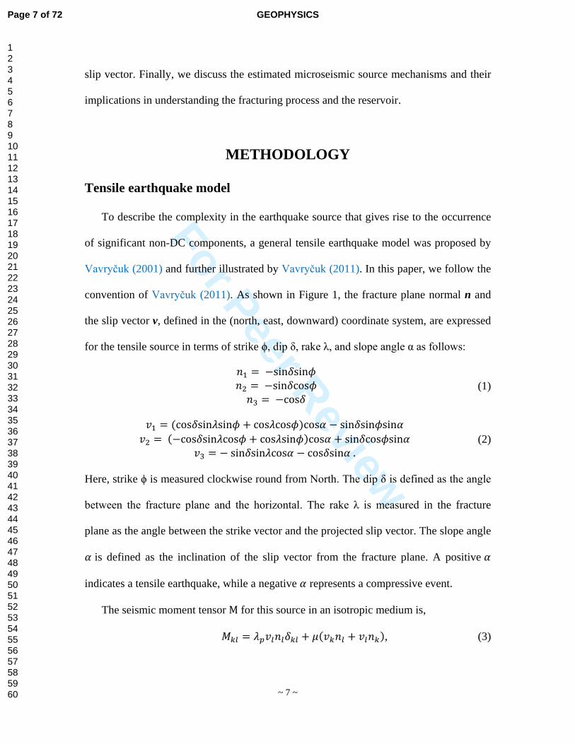
To describe the complexity in the earthquake source that gives rise to the occurrence

of significant non-DC components, a general tensile earthquake model was proposed by

Vavryčuk (2001) and further illustrated by Vavryčuk (2011). In this paper, we follow the

convention of Vavryčuk (2011). As shown in Figure 1, the fracture plane normal n and

the slip vector v, defined in the (north, east, downward) coordinate system, are expressed

for the tensile source in terms of strike ϕ, dip δ, rake λ, and slope angle α as follows:

𝑛1 = −sin𝛿sin𝜙𝑛2 = −sin𝛿cos𝜙𝑛3 = −cos𝛿

(1)

𝑣1 = (cos𝛿sin𝜆sin𝜙 + cos𝜆cos𝜙)cos𝛼 − sin𝛿sin𝜙sin𝛼𝑣2 = (−cos𝛿sin𝜆cos𝜙 + cos𝜆sin𝜙)cos𝛼 + sin𝛿cos𝜙sin𝛼

𝑣3 = − sin𝛿sin𝜆cos𝛼 − cos𝛿sin𝛼 . (2)

Here, strike ϕ is measured clockwise round from North. The dip δ is defined as the angle

between the fracture plane and the horizontal. The rake λ is measured in the fracture

plane as the angle between the strike vector and the projected slip vector. The slope angle

𝛼 is defined as the inclination of the slip vector from the fracture plane. A positive 𝛼

indicates a tensile earthquake, while a negative 𝛼 represents a compressive event.

The seismic moment tensor M for this source in an isotropic medium is,

𝑀𝑘𝑙 = 𝜆𝑝𝑣𝑙𝑛𝑙𝛿𝑘𝑙 + 𝜇(𝑣𝑘𝑛𝑙 + 𝑣𝑙𝑛𝑘), (3)


123456789101112131415161718192021222324252627282930313233343536373839404142434445464748495051525354555657585960

For Peer Review

~ 8 ~

where 𝜆𝑝 and 𝜇 are the Lamé coefficients at the focal area (to avoid confusion with fault

rake angle λ, the Lamé first parameter is denoted as 𝜆𝑝 in this paper), 𝛿𝑘𝑙 is the

Kronecker delta, 𝑛𝑙 and 𝑣𝑙 are the slip vector and fracture plane normal shown in

Equations 1 and 2, respectively. The symmetric moment tensor 𝑴 can be diagonalized

and decomposed into double-couple (DC), isotropic (ISO), and compensated linear vector

dipole (CLVD) components,

𝑴 = 𝑴𝑫𝑬𝑽 + 𝑴𝑰𝑺𝑶 = 𝑴𝑫𝑪 + 𝑴𝑪𝑳𝑽𝑫 + 𝑴𝑰𝑺𝑶. (4)

According to Vavryčuk (2011), the eigenvector b of the moment tensor matrix 𝑴

associated with the intermediate eigenvalue gives the null axis, while the eigenvectors

t and p corresponding to the maximum and minimum eigenvalues give the tension and

compression axis, respectively. The fracture plane normal v and the slip vector u can

be derived from the t and p axes after compensating for the non-zero slope angle 𝛼

(Vavryčuk, 2001) as follows:

sin𝛼 = 3 �𝜆max𝑑𝑒𝑣 + 𝜆min𝑑𝑒𝑣 � �𝜆max𝑑𝑒𝑣 − 𝜆min𝑑𝑒𝑣 �� (5)

𝒗 = 1√2�√1 + sin𝛼𝒕 + √1 − sin𝛼𝒑�, (6)

𝒏 = 1√2�√1 + sin𝛼𝒕 − √1 − sin𝛼𝒑�. (7)

λmaxdev , λmindev denote the maximum and minimum eigenvalues of the deviatoric moment

tensor 𝑴𝑫𝑬𝑽. Based on equations 1, 2, 5, 6, the source parameters, slope angle α, strike ϕ,

dip δ, and rake λ, could be determined from the moment tensor 𝑴. The ratio between the

Lamé coefficients λp and µ at the focal area is another source parameter, defined as 𝑘 and

can be derived from the moment tensor 𝑴 as follows:

𝑘 = 𝜆𝑝 𝜇⁄ = 23� 𝑡𝑟(𝑴)𝜆max𝑑𝑒𝑣 +𝜆min

𝑑𝑒𝑣 − 1� . (8)

According to Vavryčuk (2001), the stability conditions imposed on an isotropic

medium requires


123456789101112131415161718192021222324252627282930313233343536373839404142434445464748495051525354555657585960

For Peer Review

~ 9 ~

𝑘 = 𝜆𝑝 𝜇⁄ > −23 , 𝜇 > 0 . (9)

This also poses a lower limit for the Vp/Vs ratio at the focal area of the earthquakes that

follow the tensile earthquake model,

𝑉𝑝 𝑉𝑠⁄ = √𝑘 + 2 > 1.15 . (10)

According to this limit, all measurable physical properties in the focal area including Vp,

Vs, the bulk modulus and the shear modulus are positive, in spite of the fact that for some

cases, the Lamé first parameter 𝜆𝑝 may be negative.

Other source parameters including seismic moment M0, moment tensor magnitude

Mw, and DC, ISO, and CLVD component percentages could also be determined from the

moment tensor (Vavryčuk, 2001, Song and Toksöz, 2011).

Full-waveform based source mechanism determination using dual-array

data

According to our earlier study, the near-field information and nondirect waves (i.e.,

reflected/refracted waves) propagated through a layered medium contribute to the

decrease in the condition number of the sensitivity matrix, and therefore stabilize the

moment tensor inversion (Song and Toksöz, 2011). In this paper, we adopt the full

waveform inversion approach of in Song and Toksöz (2011) to determine the complete

moment tensor of microseismic events in the Barnett shale.

To reduce the influence from errors in source locations, during the moment tensor

inversion, we perform a grid search around the initial source location (Song and Toksöz,

2011). The spatial search range and grid size are selected based on the location

uncertainty. The location uncertainty in the downhole monitoring scenario is estimated

from the standard deviations of P- and S-wave arrival times and P-wave polarization


123456789101112131415161718192021222324252627282930313233343536373839404142434445464748495051525354555657585960

For Peer Review

~ 10 ~

angles (Eisner et al., 2010). For the dual-array dataset used in this study, we calculate

standard deviations and obtain 4.6 m (15 ft) in the radial direction, 7.6 m (25 ft) in the

vertical direction and 2o in P-wave derived event back-azimuths constrained by two

geophone arrays. We further determine the location uncertainty in the horizontal

directions (North, East) from the standard deviations of the radial distances and P-wave

derived event back-azimuths at a typical distance of 305 m (1000 ft) for the selected 42

events. The standard deviation is estimated to be 10.6 m (35 ft). Therefore, a spatial grid

size of 3 m (10 ft) and a spatial search cube with the size of 7*7*5 grids (North, East,

Down) are used throughout this paper.

In this study, we match full waveforms from two vertical wells. In principal, complete

moment tensor can be extracted from two observation wells for any event not situated on

the observation well plane. As pointed out by Eaton (2009), in the homogeneous medium,

the condition number of the sensitivity matrix for moment tensor inversion is inversely

proportional to the solid angle at the source subtended by the geophone array. The

nondirect waves propagated through a layered medium increase the source take-off angle

coverage and, therefore, reduce the condition number (Song and Toksöz, 2011). In either

case, an azimuthal angle at the source subtended by two vertical geophone arrays close to

90o is desirable to reduce the condition number of the sensitivity matrix. Therefore, in

this paper, we select several events that have both good SNRs and azimuthal angles to the

two geophone arrays close to 90o. In this way, low condition numbers are assured.

In this study, there was a significant difference in noise standard deviations from

geophones at different wells. Thus, a weighted least-squares inversion is performed

inside the grid search loop of event location and origin time. The weights are determined


123456789101112131415161718192021222324252627282930313233343536373839404142434445464748495051525354555657585960

For Peer Review

~ 11 ~

from the pre-event noise standard deviation at each geophone, for each component. The

weight for the n-th geophone, i-th component, 𝑤𝑛𝑖, is calculated as the inverse of the pre-

event noise standard deviation at the corresponding channel:

𝑤𝑛𝑖 = 1/𝑠𝑡𝑑�𝑛𝑖(𝑥𝑟𝑛, 𝑡)� , (11)

where 𝑛𝑖(𝑥𝑟𝑛, 𝑡) is the i-th component data of the pre-event noise at n-th geophone.

The best solution of the event location xs , origin time t0 and moment tensor Ml

( l = 1,2, … ,6 ) is determined by minimizing the squared L-2 norm of the weighted

waveform fitting error:

J(xs, t0, Ml) = ∑ ∑ ∑ w ni2 �di(xrn, kΔt) − vi(xrn, xs, kΔt)�2Nci=1

Nn=1

Ntk=1 . (12)

Equivalently, the grid search based complete moment tensor inversion is meant to

maximize the variance reduction VAR, defined as,

VAR(xs, t0, Ml) = 1 − J(xs, t0, Ml) . (13)

In this study, we noticed a poor SNR in the vertical component data, as also seen in

our earlier study (Song and Toksöz, 2011). Therefore, only horizontal components are

used in the inversion. The reasons for the poor SNRs associated with the vertical

component may come from two sources. Firstly, vertical component geophones are

normally harder to couple into the formation compared to horizontal component

geophones in a vertical borehole. Secondly, surface noise such as pumping and culture

noise coupled into the borehole propagates as guided wave modes like Stoneley-waves,

which have predominant motion in the vertical component.

FIELD STUDY

An overview of the Barnett gas shale reservoir


123456789101112131415161718192021222324252627282930313233343536373839404142434445464748495051525354555657585960

For Peer Review

~ 12 ~

The Fort Worth Basin was bordered on its outboard side by an island-arc system

which supplied very little coarse-grained sediment to the Barnett Shale. Limestone

interbeds in the Barnett (including the middle Forestburg Member) formed as mass-

gravity or turbidity flows of skeletal material derived from surrounding carbonate

platforms. Immediately after black-shale deposition, a temporary expansion of the

western carbonate produced the overlying Marble Falls Formation. The Mississippian

stratigraphic section in the Fort Worth Basin consists of limestone and organic-rich shale.

The Barnett Shale formation, in particular, consists of dense, organic-rich, soft, thin-

bedded, petroliferous, fossiliferous shale and hard, black, finely crystalline, petroliferous,

fossiliferous limestone (Lancaster et al., 1993).

The Barnett Shale, as determined by core and outcrop studies, is dominated by clay-

and silt-size sediment with occasional beds of skeletal debris. In lithologic descriptions,

the Barnett shale is a mudstone rather than shale. It is highly indurated, with silica

making up approximately 35–50% of the formation by volume and clay minerals less

than 35% (Bruner and Smosna, 2011). This silica-rich nonfissile shale behaves in a more

brittle fashion and fractures more easily than clay-rich shales, responding well to

stimulation.

The Barnett shale reservoir has characteristic features of very low matrix permeability

in the range of microdarcies to nanodarcies (Johnston, 2004), and some degree of natural-

fracture development (Bruner and Smosna, 2011). From core studies, two major sets of

natural fractures were identified. One fracture system had an azimuth of north-south (N-S)

and another, west-northwest-east-southeast (WNW) (Gale et al., 2007; Gale & Holder,


123456789101112131415161718192021222324252627282930313233343536373839404142434445464748495051525354555657585960

For Peer Review

~ 13 ~

2010). Surprisingly the natural fractures in the Barnett shale were completely healed and

filled with calcites.

Field setup

A microseismic survey using two vertical wells at a separation of about 487 m (1600

ft) was conducted during the waterfrac treatment of the Barnett shale in the Fort Worth

Basin at depths of about 2290 m (7500 ft). Each observation well had twelve-level, three-

component geophones spaced approximately 12 m (40 ft) apart, with the tool situated just

above the shale interval that was being stimulated. The recorded data were analyzed and

located for hydraulic fracturing mapping as outlined by Warpinski et al. (2005). The

velocity model for location, shown in Figure 2a, was derived from the well logging data

and calibrated using perforation shots. The information on local geology was also

considered when building the velocity model.

A typical anisotropy parameter for the Barnett shale is reported as ε = 0.1,Δ =

0.2, γ = 0.1 (note that the Thomsen parameter which controls the near-vertical

anisotropic response is denoted as Δ in this paper to avoid the confusion with fracture dip

angle δ) (Warpinski et al., 2009). From the examination of the ray paths from all

microseismic events to two geophone arrays, it is found that the ray paths are mostly

horizontal, with a maximum deviation from the horizontal less than 22o (Warpinski et al.,

2009). According to the weak anisotropy theory of Thomsen (1986), the P-wave velocity

variation within this range would be less than 0.5%, while the SH velocity variation

would be less than 2%. Therefore, we may conclude that, for this dataset, the effect of

anisotropy on the waveform modeling is small relative to the general uncertainty in

velocity. In the study, the perforation-calibrated horizontal velocity model described in


123456789101112131415161718192021222324252627282930313233343536373839404142434445464748495051525354555657585960

For Peer Review

~ 14 ~

Figure 2a is used and the anisotropy effect is neglected. Table 1 lists the seismic

properties of the layer sequence in the Barnett shale reservoir, which are used to generate

synthetic seismograms for moment tensor inversion. The density information is extracted

from the density log. The P- and S-wave Q factor values are determined by considering

both the lithology and amplitude decay measured across the geophones (Toksöz and

Johnson, 1981; Rutledge et al., 2004).

Figure 3 gives the horizontal plane view of the microseismic event locations from

waterfrac treatment in the Barnett shale using the isotropic velocity model shown in

Figure 2a. The majority of the microseismic events occur in the lower Barnett shale

interval. The two vertical observation wells 1 and 2 are presented as the yellow and green

squares on Figure 3, respectively, while the treatment well trajectory is plotted as the

cyan line with treatment wellhead shown as the blue square. The origin (0, 0) corresponds

to the location of observation well 1. The green dashed line represents the observation

well plane. As stated previously in the methodology section, we select several events that

have both good SNRs and azimuthal angles to the two geophone arrays close to 900 for

complete moment tensor inversion. A total of 42 events are selected. Among the chosen

events, 4 event groups appear and are denoted as G1, G2, G3, and G4, respectively.

In the following section, we will follow the processing flow proposed in the

methodology section, and conduct a systematic study to evaluate the uncertainty of the

inverted source parameters for each event group using synthetic data. After that, we will

proceed to the geomechanical analysis section to gain some insights on how the

microearthquakes are generated. We will also propose an approach to distinguish the

fracture plane from the auxiliary plane. Finally, we will discuss the field study results.


123456789101112131415161718192021222324252627282930313233343536373839404142434445464748495051525354555657585960

For Peer Review

~ 15 ~

Uncertainty of the inverted source parameters from synthetic study

In this section, we study the influence of velocity model errors, source mislocations

and additive data noise on the inverted source parameters by performing a Monte-Carlo

test using synthetic data.

Firstly, we study the influence of data noise and source mislocations. In this test, we

generate noise-free synthetic seismograms for each example event within the four event

groups using the reference velocity model shown in Figure 2a to mimic the field case.

Without losing generality, four tensile earthquakes with (ϕ, δ, λ, α, 𝑘) of (60o, 80o, 60o,

20o, -0.3), (30o, 75o, -160o, 15o, 0.8), (55o, 85o, 80o, 25o, -0.5), and (10o, 50o, 75o, -20o, 0.1)

were simulated to represent events for group G1, G2, G3, and G4, respectively. The

double-couple component percentages for each of these four tensile earthquakes are 53%,

51%, 48% and 48%. The same source model is used throughout the synthetic study

section. It is worth noting that a larger slope angle α is chosen with a higher dip δ in this

model. The motivation for this choice will be further illustrated in the geomechanical

analysis section.

For each well, the noisy synthetic data were formed by adding zero-mean Gaussian

noise with a standard deviation reaching 10% of the absolute maximum amplitude of the

two horizontal components averaged across the twelve geophones. The noise was added

independently for each geophone array at the same noise level of 10%. The noise level of

10% was set to represent the estimated noise level in the field dataset.

To investigate the influence of source mislocations, the true event location is

randomly perturbed up to 10.6 m (35 ft) in each horizontal direction and 7.6 m (25 ft) in

the vertical direction to represent the location uncertainty in the field example. In the


123456789101112131415161718192021222324252627282930313233343536373839404142434445464748495051525354555657585960

For Peer Review

~ 16 ~

inversion, a grid search is carried out around the perturbed event location. The moment

tensor inversion is performed on the [100, 300] Hz band-pass filtered noisy synthetic data

using the correct velocity model. The moment tensor solution corresponding to the

minimum L-2 waveform fitting error is selected as the inversion result. The source

parameters are then estimated from the inverted complete moment tensor. In all synthetic

tests, we distinguish the fracture plane from the auxiliary plane by selecting the one with

a smaller error in source parameter estimates. However, in the field study section, where

no knowledge about the true source parameters is available, we will propose a method to

distinguish the fracture plane from the auxiliary plane according to the insights from the

geomechanical analysis.

In order to obtain statistically relevant results, we perform 100 moment tensor

inversions and source parameter estimations, each with a different noise realization.

Table 2 summarizes the average absolute errors of the inverted source parameters for four

example events. The condition number of the sensitivity matrix for each example event

from the weighted least squares inversion is also listed. The example event G4 has the

largest condition number due to the smallest azimuthal angle at G4 subtended by the two

geophone arrays, which is seen on Figure 3. Overall, the inverted source parameters agree

well with the true values, with average absolute errors in both FPS and slope angle α less

than 2 degrees. The average absolute errors in component percentages, 𝑘, and M0 are also

negligible. This indicates that with a correct velocity model, microseismic source

mechanisms can be reliably determined from the dual-array dataset by the grid search

based full waveform inversion approach, as long as the event mislocation is within the

location uncertainty and the condition number is reasonably low. Additive data noise has


123456789101112131415161718192021222324252627282930313233343536373839404142434445464748495051525354555657585960

For Peer Review

~ 17 ~

a minimal effect on the inversion, which is also reported in Song and Toksöz (2011). It is

interesting to point out that, at the same noise level, errors in the inverted source

parameters tend to be higher at a larger condition number. This is reasonable, since the

errors propagated into the moment tensor solution from data noise are controlled by the

condition number.

Next, we perform the DC inversion instead of complete MT on the same band-pass

filtered noisy synthetic data. In this inversion, the event source mechanism is forced to be

double-couple. Therefore, it provides no information on α, 𝑘, and component percentages.

Table 3 lists the average absolute errors of the inverted seismic moment and FPS for four

example events. Compared to Table 2, it is clear that DC inversion severely biased the

estimates of fracture plane orientation even with a correct velocity model. This is

understandable, since the DC source clearly is not a good assumption about the

underlying tensile earthquakes, which have a DC component percentage of only about

50%.

Finally, we investigate the influence of velocity model errors on the inversion. In this

test, the P- and S-wave velocity models are randomly perturbed up to 10% and 20% of

the velocity difference between adjacent layers so that the sign of the velocity difference

between adjacent layers does not change. A larger perturbation for S-wave velocity is to

take into account the fact that the S-wave velocity is generally less reliably determined

than the P-wave velocity. The perturbation is independent between different layers and P-

and S-wave velocities are independently perturbed. The density model is kept unchanged,

as the velocity perturbation is dominant in determining the characteristics of the

waveforms. The Qp and Qs model is also kept constant to study the influence of the


123456789101112131415161718192021222324252627282930313233343536373839404142434445464748495051525354555657585960

For Peer Review

~ 18 ~

velocity perturbation. The velocity models are perturbed 100 times, as shown in Figure

2b. We then conduct 100 moment tensor inversions and source parameter estimations,

each with a different velocity model and noise realization. In each inversion, the 10%

Gaussian noise and the same amount of source mislocations as the case for Table 2 are

also included.

Figure 4 demonstrates the process of the grid search based moment tensor inversion

of the synthetic tensile event G1 for one velocity model and noise realization. It plots the

normalized variance reduction as a function of searched event location and origin time.

The black star denotes the initial source location and origin time estimate, while the white

star gives the source location and origin time after full waveform matching. It is clear that

the variance reduction function VAR is maximized at the inverted source location and

origin time, suggesting a better waveform fit than the initial event location and origin

time. The moment tensor solution, event location, and origin time are then determined.

Figure 5 shows the best waveform fitting for the synthetic event G1. A good agreement

between modeled data in black and band-pass filtered synthetic data in red is seen on

both components.

100 moment tensor inversions, each with one inaccurate velocity model and noise

realization, are performed to study the influence of velocity model errors on the inverted

source parameters. Figure 6 plots the errors of the inverted event location along (N, E, D)

directions in stars for the synthetic tensile source G1 as a function of different velocity

model realizations. The event location error is shown as multiples of search grid size. The

black line represents the search limit in the vertical direction for the grid search based

moment tensor inversion, while the green line demonstrates the identical search limit in


123456789101112131415161718192021222324252627282930313233343536373839404142434445464748495051525354555657585960

For Peer Review

~ 19 ~

the north and east directions. It is observed that all the location errors are bounded in the

search limit. This indicates that our search range is sufficient for the assumed velocity

model errors. Figure 7 gives the histograms of errors in the inverted source parameters

for the synthetic event G1.

Likewise, Figure 8 gives the best waveform fitting for the synthetic event G4, which

is located close to well 2 and far from well 1. A good agreement between modeled data in

black and band-pass filtered synthetic data in red is also observed on both components.

This indicates the effectiveness of weighted least squares inversion in dealing with the

significant difference in noise standard deviation at different geophone arrays. Figure 9

plots the histograms of errors in the inverted source parameters for the synthetic event G4.

A similar Monte-Carlo test was also conducted for synthetic events G2 and G3. Table

4 summarizes the average absolute errors of the inverted source parameters for all 4

synthetic events. The median value of the condition number of the inversion matrix

across the 100 inversions is also listed for each example event. Three observations are

seen in Table 4. Firstly, compared to Table 2, the errors in the inverted source parameters

are clearly increased for all events. This signifies that the velocity model errors have a

more profound influence in the moment tensor inversion than data noise and source

mislocations. Secondly, at the same noise level and with the same amount of velocity

model perturbations, the example event with the smallest median condition number

(event G3) tends to have the least error in source parameter estimates. For the assumed

velocity model errors, the event G1, with the largest condition number, has an average

absolute error of 0.9, 14o, 22o and 21% for 𝑘, α, ϕ and CLVD component percentage,

respectively. Finally, among all 4 inverted source parameters (ϕ, δ, λ, α) related to the


123456789101112131415161718192021222324252627282930313233343536373839404142434445464748495051525354555657585960

For Peer Review

~ 20 ~

fracture plane orientation and slip direction, the dip angle δ is the most reliably

determined, with a maximum error up to 5o, while the strike angle ϕ is the least accurate

estimate. The errors in the inverted slope angle α are also small, indicating that α can be

accurately estimated.

Hydraulic fracture geomechanics in the Barnett shale

To understand how microearthquakes are generated in the Barnett shale, it is essential

to look at the hydraulic fracture mechanics. Microseismicity associated with hydraulic

fracturing has considerably different geomechanical aspects than tectonic earthquakes,

rockbursts, or geothermal shear dilation. The inflation of a hydraulic fracture with

internal pressure induces very large stresses in the surrounding formation. The stress

perturbations are often greater than the stress difference that existed in the formation

prior to fracturing. In addition, the leakoff of the high pressure fluid, at pressures well

above the minimum in situ stress, reduces the normal stress and destabilizes any natural

fractures or other permeable weakness planes. These combined factors create the unstable

zones around the hydraulic fracture where the microseismicity would occur (Warpinski et

al., 2012). In this section, we calculate the hydraulic fracture induced stress perturbations

in the Barnett shale and consider the pore pressure increase resulting from fracturing fluid

leakage to study possible failure types that could occur in the Barnett shale.

Looking at a single hydraulic fracture for simplicity, there are several models

available to calculate the stress field induced by the fracture, including both finite

element and analytical models. For scoping calculations, analytical models are sufficient.

Among the various analytical models, the most versatile one is a pressurized three-

dimensional (3D) elliptic crack (Green and Sneddon, 1950). This model requires a


123456789101112131415161718192021222324252627282930313233343536373839404142434445464748495051525354555657585960

For Peer Review

~ 21 ~

homogeneous, isotropic, linear-elastic formation and a uniform fluid pressure inside the

hydraulic fracture, but these simplifications still allow for adequate evaluation of the

characteristics of the stress field around the hydraulic fracture and the influence of the

stress field on rock failure behavior. As described in Figure 10, the stress perturbations

have two characteristic zones, a tip-influenced region along the hydrofracture tip

direction and a broadside region along the hydrofracture normal direction, and these are

considered separately. Prior to fracturing, the Barnett shale reservoir is in the normal

faulting regime (Bruner and Smosna, 2011; Agarwal et al., 2012). Therefore, the

broadside region is along the unperturbed minimum horizontal principal stress (Shmin)

direction and the tip region is along the unperturbed SHmax direction. Only a vertical

fracture is considered here.

Table 5 lists the hydrofracture and formation parameters typical of the Barnett shale

waterfrac treatment (Agarwal et al., 2012). The broadside region, the area alongside the

hydrofracture after the tip has passed, can be assessed using the analytic model of Green

and Sneddon (1950) for typical elongated fractures (length > height). Figure 11a gives the

stress decay moving away from the hydrofracture face along the centerline of the

hydrofracture, with respect to both length and height. The largest stress perturbation is

the compressive stress along the Shmin direction. While the stress perturbation in the

SHmax direction is also compressive, it is considerably less. This behavior suggests the

stress perturbations imposed by the hydrofracture are highly stabilizing in the broadside

region. The reason is twofold. First, the shear stress in the formation is significantly

reduced since the horizontal differential stress is decreased after the hydrofracture

perturbation. Second, the total normal stress is increased, since compressive stress is


123456789101112131415161718192021222324252627282930313233343536373839404142434445464748495051525354555657585960

For Peer Review

~ 22 ~

added to both SHmax and Shmin stresses. The combined effect is to increase frictional

strength and reduce the available shear stress, making it very difficult for

microearthquakes to occur. One possibility to generate microseismicity in the broadside

region is to have the high pressure fracturing fluid leak off into permeable weak zones

such as natural fractures, since the increase in the pore pressure from fluid leakage will

destabilize the weak zones and cause microearthquakes to happen (Warpinski et al.,

2012). For an over-pressured gas reservoir such as the Barnett shale reservoir, the pore

pressure increase resulting from fracturing fluid leakage is actually much greater than the

stress perturbation due to the opening of the hydrofracture, since the pore pressure change

is on the order of the fracturing pressure minus the ambient pore pressure, while the stress

change, the net pressure, is on the order of the fracturing pressure minus the unperturbed

Shmin stress.

The tip region of the hydrofracture has a different stress perturbation pattern. Figure

11b plots the stress perturbations due to the presence of the hydrofracture ahead of the

length tip along the centerline of the hydrofracture with respect to height and width. Here,

all the stress changes are tensile. The largest tensile stress is along the SHmax direction,

and a slightly smaller tensile stress occurs along the Shmin direction. This has the effect

of slightly decreasing the horizontal differential stress and significantly decreasing the

total stress. The net effect could be destabilizing the tip region and inducing

microearthquakes if any favorably oriented weakness planes are encountered. This zone

is relatively small, at most a few meters, and provides a mechanism for microearthquakes

to occur slightly ahead of the hydrofracture tip. In contrast to the broadside region, there

is no fluid leakage in this zone, and therefore the pore pressure stays as the ambient pore


123456789101112131415161718192021222324252627282930313233343536373839404142434445464748495051525354555657585960

For Peer Review

~ 23 ~

pressure. The above calculations are related to a single hydraulic fracture. Although the

geomechanics become considerably more complex in the case of multiple hydraulic

fractures during the multiple-stage, multiple-perforation treatment, the general features of

stress perturbations from the single hydraulic fracture analysis still hold (Warpinski et al.,

2012; Agarwal et al., 2012).

Fischer and Guest (2011) proposed a way to identify four different types of

earthquakes as shown in Figure 12: tensile (𝜎𝑛 < 0 , 𝜏 = 0 , α > 0 ), hybrid tensile

(𝜎𝑛 < 0, |𝜏| > 0, α > 0), pure shear (𝜎𝑛 = 0, |𝜏| > 0, α = 0) and compressive shear

(𝜎𝑛 > 0, |𝜏| > 0, α < 0) events. The Mohr circle was used to represent in-situ stress state,

and the Griffith failure criterion was adopted to describe both shear and tensile failures

(Ramsey and Chester, 2004). The Griffith failure criterion reads

𝜏2 = 4𝑇0(𝜎𝑛 + 𝑇0) , (14)

𝑆0 = 2𝑇0 , (15)

where S0 and T0 are the inherent cohesion strength and the tensile strength of the rock.

According to the Griffith failure criterion, rock will fail along a fracture plane where the

shear stress τ reaches the level specified by equation 14.

Only the fluid leakage effect was considered by Fischer and Guest (2011). However,

the stress perturbations from the hydrofracture are important for the analysis of

microseismicity associated with hydraulic fracturing (Warpinski et al., 2012). In this

study, we take into account both the fluid leakage effect and stress perturbations due to

the presence of the hydrofracture. We consider two possibilities, microseismicity

occurring in the intact rock and on the weak zones such as natural fractures and induced

hydraulic fractures.


123456789101112131415161718192021222324252627282930313233343536373839404142434445464748495051525354555657585960

For Peer Review

~ 24 ~

Different cohesion strength values were proposed to describe the intact rock and the

weak zones inside the Barnett shale. The cohesion strength is normally derived from the

tensile strength according to equation 15. It is generally accepted that the tensile strength

value is highly variable. In Gale and Holder (2008), a tensile strength value ranging from

12 to 44 MPa was reported for the Barnett shale samples tested, while in Tran et al.

(2010), a tensile strength value of the Barnett shale ranging from 1.38 MPa (200 psi) to

20.7 MPa (3000 psi) was proposed. In this study, we found that a tensile strength of 10

MPa for the intact rock and 1 MPa for the weak zones inside the Barnett shale seems to

adequately explain the observed microseismicity. The core analysis indicates that the

natural fractures inside the Barnett shale are calcite filled while the rock matrix is mostly

siliceous, suggesting a weak bond between the calcite filling and the surrounding rock

matrix (Gale et al., 2007). Therefore, a one-tenth of the tensile strength of the intact rock

is assigned as the tensile strength of the natural fractures in this study. The difference

between the tensile strength of the intact rock used in this paper and that reported by Gale

and Holder (2008) may be attributed to the scale effect and possible data selection bias in

the laboratory study. The observed microseismicity typically occurs at a much larger

scale than the size of core samples used in the laboratory test. Moreover, stronger rock

samples with higher tensile strengths are easier for laboratory testing, and thus may incur

the data selection bias. Overall, the parameters used for the geomechanical analysis of the

Barnett shale are listed in Table 5.

In Figure 13a, the 3D Mohr-circle shows the locus of the shear stress 𝜏 and the

effective normal stress 𝜎𝑛 on an arbitrarily oriented fracture in the Barnett shale. The blue

circle on the right corresponds to the ambient pore pressure p0, while the left circle is


123456789101112131415161718192021222324252627282930313233343536373839404142434445464748495051525354555657585960

For Peer Review

~ 25 ~

associated with the maximum possible pore pressure case, that is, when the pore pressure

is elevated to the fracturing pressure pf. The Griffith failure envelope for the intact rock

with the inherent cohesion strength S0 of 20 Mpa is plotted in Figure 13a as the red curve.

It is discovered that even at the maximum possible pore pressure, rock failure is very

unlikely to occur in the intact rock because of its large cohesion strength. It is worth

mentioning that only pore pressure increase is considered here, since the pore pressure

increase resulting from fracturing fluid leakage is actually much greater than the stress

perturbation due to the opening of the hydrofracture under the treatment parameters listed

in Table 5.

Figure 13b gives the failure analysis in the tip region. In this region, no fracturing

fluid leakage occurs. According to Figure 11, the stress perturbations due to the hydraulic

fracture are assumed to be −0.77𝑝𝑛𝑒𝑡, −𝑝𝑛𝑒𝑡 and −0.1𝑝𝑛𝑒𝑡 along the Shmin, SHmax and

vertical directions, respectively. The black, green and cyan crosses denote the principal

stresses in the original unperturbed Shmin (NW-SE), SHmax (NE-SW) and vertical

directions, respectively. It is interesting to see that the relative magnitude of the Shmin

and SHmax principal stresses has changed due to the stress perturbation from the

hydraulic fracture. The original Shmin (NW-SE) direction is now becoming the

maximum in-situ horizontal stress direction. The Griffith failure envelope for the weak

zones inside the Barnett shale with the inherent cohesion strength S0w of 2 Mpa is plotted

as the red curve. It is found from Figure 13b that compressive shear events could happen

on some preferred weak zones in the tip region. As described in Figure 13b, the angle

between the failure point and the maximum principal stress σv is equal to 2δ, that is,

twice the dip angle of the fracture plane (Zoback, 2007). This suggests that compressive


123456789101112131415161718192021222324252627282930313233343536373839404142434445464748495051525354555657585960

For Peer Review

~ 26 ~

shear events (α < 0) with a dip around 50o could occur on weak zones such as natural

fractures in the tip region.

Figure 14a presents the failure analysis in the broadside region. The stress

perturbations from the hydraulic fracture are assumed to be +0.5pnet, +0.1pnet and 0 in

the Shmin, SHmax and vertical directions, respectively. The decrease of horizontal

differential stress, together with the increase in the total stress, stabilizes the broadside

region. Therefore, the fracturing fluid leakoff into the weakness zones is essential for

microearthquakes to occur in this region. The pore pressure increase is assumed to be

equal to the net fracturing pressure pnet minus a pressure drop term. The pressure drop is

inversely proportional to the square root of the permeability of the natural fractures,

which is unknown. In Figure 14, a pressure drop of 200 psi is assumed, as suggested by

Agarwal et al. (2012). The selection of this value is not intended to estimate the pressure

drop but to serve as a scoping parameter. The black, green and cyan crosses denote the

principal stresses along the original unperturbed Shmin (NW-SE), SHmax (NE-SW) and

vertical directions, respectively. The interchange of Shmin and SHmax directions

resulting from the hydrofracture induced stress changes is also seen. The red, green and

blue pluses demonstrate the shear and effective normal stresses on the fracture planes

with strike angles of (80o, 140o), (10o, 70o), and (-15o, 45o), respectively (corresponding

to a +/- 30o range around the WNW, N-S, NW-SE directions). The corresponding dip

angles are also listed in the figure. The Griffith failure envelope for the weak zones with

the inherent cohesion strength S0w of 2 Mpa is plotted as the red curve. It is observed in

Figure 14a that both compressive shear and tensile events could happen on some

preferred fractures in the broadside region with the existence of fluid leakage. Similar to


123456789101112131415161718192021222324252627282930313233343536373839404142434445464748495051525354555657585960

For Peer Review

~ 27 ~

Figure 13, because of the decreased horizontal differential stress after hydrofracture stress

perturbation, the 3D Mohr circle behaves like a 2D Mohr circle with almost identical

principal stresses in Shmin and SHmax directions. Therefore, for reservoirs with a low

horizontal differential stress and in normal faulting regimes, such as the Barnett shale

reservoir, rock failure could occur along almost any strike direction. However, the

fracture plane dip angle does play an important role in determining the failure type.

Figure 14b gives the zoomed version of Figure 14a. It is clear that in spite of different

strike angles, tensile events could only occur at high dip angles such as δ= 80o in this

figure, while compressive shear events are observed at a low dip angle like δ= 45o.

It is worth pointing out that the stress perturbation values chosen for the tip and

broadside region in the analysis above are not meant to be an accurate representation of

the in-situ stress changes but to serve as the typical scoping parameters. Nevertheless,

some general conclusions regarding microseismicity in the Barentt shale can still be

drawn. Firstly, microseismicity is very unlikely to occur in the intact rock because of its

large cohesion strength. Therefore, weak zones like natural fractures are critical for

hydraulic fracturing in the Barnett shale (Gale et al., 2007; Gale & Holder, 2010).

Secondly, rock failure could happen on the preferred weak zones in both the tip region

and the broadside region. The pore pressure increase due to fracturing fluid leakage is

essential for microseismicity in the broadside region, while tensile stress perturbations

incurred by the hydraulic fracture facilitate the generation of microearthquakes in the tip

region. Possible weak zones in the Barnett shale include natural fractures and the newly

created hydraulic fractures. Two sets of dominant natural fractures were reported to be in

the WNW and N-S directions, respectively (Gale et al., 2007; Gale & Holder, 2010).


123456789101112131415161718192021222324252627282930313233343536373839404142434445464748495051525354555657585960

For Peer Review

~ 28 ~

Finally, for reservoirs with a low horizontal differential stress and in normal faulting

regimes, such as the Barnett shale reservoir, rock failure could occur along almost any

strike direction. The tensile events tend to occur at high dip angles, while compressive

shear events are normally associated with low dip angles. This observation suggests that

we could assign the high dipping plane as the fracture plane for tensile events and treat

the low dipping plane as the fracture plane for compressive shear events. This justifies

the synthetic sources we assumed in the previous synthetic study section. In the following

field study section, we will use this approach to distinguish the fracture plane from the

auxiliary plane.

Moment tensor inversion and source mechanism determination: results

and discussions

In this section, we apply the grid search based full waveform inversion approach to

the 42 selected events to invert for the complete moment tensor. The tensile earthquake

source parameters including FPS (strike ϕ, dip δ, rake λ), the slope angle α, 𝑘, the Vp/Vs

ratio at the focal area, seismic moment M0, moment tensor magnitude Mw, and DC, ISO,

and CLVD component percentages are also estimated from the inverted moment tensors.

We will begin with one field event, named ‘G1-1’, to demonstrate the procedure of the

complete moment tensor inversion and source parameter estimation using full waveforms.

After that we will present the source mechanism results for all 42 chosen events and

discuss their implications in understanding the fracturing process and the reservoir.

Figure 15 demonstrates the process of the grid search based moment tensor inversion

of the field event G1-1 using the layered model illustrated in Table 1 and Figure 2a. On

Figure 15a, the normalized variance reduction is plotted as a function of searched event


123456789101112131415161718192021222324252627282930313233343536373839404142434445464748495051525354555657585960

For Peer Review

~ 29 ~

location and origin time. The black star denotes the initial source location and origin time

estimate, while the white star gives the inverted source location and origin time. It is clear

that the variance reduction function VAR is maximized at the inverted source location

and origin time, suggesting a better waveform fit than the initial event location and origin

time. Figure 15b presents the VAR at the inverted source location as a function of origin

time. It is observed that the VAR is periodical with respect to the time shift. A

comparison between Figure 15a and Figure 15b seems to indicate that the periodicity of

VAR with respect to the time shift is more pronounced than that to the source location.

This is caused by inverting seismograms of a limited frequency band between 100 and

300 Hz. A wider frequency band gives a better resolution but a less stable inversion result.

This is because a larger frequency bandwidth requires a more accurate velocity model

and an energetic signal across a wide frequency band, which is difficult to achieve in the

field. Therefore, the selection of the filtering bandwidth of [100, 300] Hz is to balance the

tradeoff between the inversion stability and the solution resolution.

The moment tensor solution, event location, and origin time are then determined.

Figure 16 shows the best waveform fitting for the field event G1-1. A good agreement in

dominant P- and S-wave trains between modeled data in black and observed data in red is

seen on both components. It is worth pointing out that the noisy feature on the modeled

data of well 2 in Figure 16a is not due to numeric noise but as a result of the large scaling

factor of 11.65 used in the plot. The actual waveform amplitude of the North component

from well 2 is much smaller than that from well 1. In this example event, we did not

notice significant unmodeled wave packages. In some other events, we did see some

degree of unmodeled wave packages between P- and S-arrivals, which probably points to


123456789101112131415161718192021222324252627282930313233343536373839404142434445464748495051525354555657585960

For Peer Review

~ 30 ~

the presence of a complex laterally inhomogeneous structure in this area. Overall, a good

agreement in dominant P- and S-wave packages between modeled data and observed data

is observed for all 42 events.

Next, we estimate the source parameters from the inverted moment tensor for this

field event G1-1 using the method proposed in the methodology section. Two planes with

strike, dip and rake of (16o, 79o, 70o), (343o, 32o, 229o) are derived. The slope α is

estimated to be 37o. Even considering the possible error of 14o in the slope angle due to

data noise, source mislocations and velocity model errors as discussed in the synthetic

study, the field event G1-1 is considered to be tensile. Moreover, as illustrated in the

synthetic study, the dip angle is the most reliably determined parameter (see the analysis

in Table 4). Therefore, the plane with the larger dip angle of 79o is selected as the fracture

plane following the conclusion drawn from geomechanical analysis. The fracture strike is

estimated to be 16o. As illustrated in the synthetic study, the strike angle ϕ is the least

accurate source parameter estimate with an error up to 22o for event group G1 (see Table

4). The fracture strike associated with field event G1-1 is considered to be consistent with

the N-S direction. Therefore, event G1-1 is attributed to the tensile opening of the N-S

natural fracture.

To further confirm the non-DC components presented in event G1-1, the F test has

been performed to test the significance of non-DC components by taking into account the

variance reductions in the MT and pure DC inversions, and the corresponding numbers of

degrees of freedom in the observed data (Šílený et al., 2009). It turns out for event G1-1,

at a confidence level of 99.9%, the MT model is better than the DC source model in

satisfying the observed data. Actually, for all the 42 events under investigation, at a


123456789101112131415161718192021222324252627282930313233343536373839404142434445464748495051525354555657585960

For Peer Review

~ 31 ~

confidence level higher than 95%, the MT model is preferred to describe the observed

data. In other words, the probability of the existence of the non-DC source is significant.

The same procedure is then applied to all the selected events. Table 6 summarizes the

determined source parameters for all 42 events. It is observed that all the events except

the 6 underlined events follow the tensile earthquake model. The 6 underlined events

have k values beyond the physical limit described in equation 9 and, therefore, cannot be

modeled by the tensile earthquake model of Vavryčuk (2001). The reason for this

behavior is not clear. It may be due to the higher complexity in these 6 events that cannot

be modeled by the simple tensile earthquake model. Nevertheless, we will focus our

attention on the remaining 36 events in the following discussion.

Considering the possible error in the strike estimate as described in the synthetic

study (see Table 4), we group the 36 events in Table 6 into 3 groups: 11 events striking in

the NE-SW direction are shown in black (“black events” hereinafter), 3 events striking

along the WNW direction are depicted in blue (“blue events” hereinafter), and the

remaining 22 events striking approximately along the N-S direction are listed in red (“red

events” hereinafter). As mentioned previously, Gale et al. (2007) identified two sets of

dominant natural fractures along the WNW and N-S directions, respectively. Pre- and

post-injection borehole image logs and cored intervals suggest that, in structurally

complex areas, multiple hydraulic fracture strands are likely to propagate along the

SHmax direction (Warpinski et al., 1993, Fast et al., 1994). Geologic discontinuities,

such as joints, faults, and bedding planes, were found to contribute to the creation of

multiple hydraulic fracture strands mapped during mineback experiments and generated

in laboratory tests (Warpinski and Teufel, 1987). Recently, numerical studies also


123456789101112131415161718192021222324252627282930313233343536373839404142434445464748495051525354555657585960

For Peer Review

~ 32 ~

indicate that the interaction between pre-existing natural fractures and the advancing

hydraulic fracture is a key condition leading to complex hydraulic fracture patterns

(Dahi-Taleghani and Olson, 2011). Therefore, it is likely that multiple hydraulic

fractures oriented sub-parallel to the SHmax direction, i.e. the NE-SW direction, would

form because of the interaction of the main advancing hydraulic fracture and pre-existing

natural fractures in the Barnett shale. Hence, we may attribute the identified 3 groups of

events in black, blue and red to rock failures on the hydraulic fractures in the NE-SW

direction, the WNW and N-S oriented natural fractures, respectively.

It is observed in Table 6 that all 11 black events striking along the NE-SW direction

have positive slope angles. Even if the possible errors in the slope estimate are considered,

at least 9 black events have non-negligible positive slope angles, despite that the other 2

black events have slope angles close to 0o. It is believed that these events striking along

the NE-SW direction may indicate the tensile opening of multiple hydraulic fractures

trending sub-parallel to the SHmax direction.

The fracture plane orientation of the blue and red events is close to the natural

fracture orientation. It is speculated that these events correspond to the reactivation of

WNW and N-S oriented natural fractures. The majority of these events have positive

slope angles, in spite of the possible errors in the slope estimate as described in Table 4.

This seems to indicate the existence of tensile opening associated with the reactivation of

natural fractures. Nevertheless, non-negligible negative slope angles are also seen for

some blue and red events, such as events G1-3, G1-11, G1-14, G1-18, G3-1 and G3-3.

One question arises, that is, how could these compressive shear events on natural

fractures improve the permeability and enhance gas production? One possible


123456789101112131415161718192021222324252627282930313233343536373839404142434445464748495051525354555657585960

For Peer Review

~ 33 ~

explanation would be the fracture asperity. The shearing process causes the calcite filling

inside the natural fractures to break, which creates open spaces. The compressive stress

may decrease the volume of the newly created void space, but the asperities in these

natural fractures help preserve some of the newly created flow paths and, therefore,

support an increase in permeability.

The moment magnitude for all the events is found to range from 0 to -3, with the

majority falling into the range of -1 to -3, even after taking into account a possible error

in seismic moment estimate up to 30%.

It is observed in Table 6 that the Vp/Vs ratio in the focal area is generally lower than

that of the surrounding medium where seismic waves propagate. This behavior was also

reported in the seismological study of tensile faulting by Fojtíková et al. (2010). It is also

interesting to see that some of the largest derived Vp/Vs ratios (Vp/Vs >1.7 for events

G4-8, G1-17, G2-2) appear in the events occurring on the hydraulic fractures trending

sub-parallel to the SHmax direction. Even considering the possible uncertainty in the k

estimate resulting from data noise and velocity model inaccuracies, this observation still

holds. These large Vp/Vs ratios, close to that of the surrounding medium, might be a sign

of newly formed hydraulic fractures instead of aged natural fractures.

Furthermore, in terms of component percentages, many events from the group G1, G4

seem to have CLVD as the dominant component. Two possible reasons for this behavior

are (1) errors in CLVD component and (2) the mechanism associated with hydraulic

fracturing in these complex fractured gas shales.

The possibility of a large error in CLVD component percentage for event groups G1

and G4 is very real because of their larger condition numbers, as seen from Table 4.


123456789101112131415161718192021222324252627282930313233343536373839404142434445464748495051525354555657585960

For Peer Review

~ 34 ~

There may also be a possibility of data selection bias. Good quality events generally have

good P-waves, but P-waves are quite small for pure DC events.

Alternatively, for some events in the groups G1 and G4, the analysis might be correct

and a large CLVD component may be physical, reflecting the properties of the

earthquake source or of the medium in the focal area. On one hand, this could be an

indicator of the presence of tensile faulting, manifested by a positive correlation between

the ISO and CLVD components (Vavryčuk, 2001). On the other hand, the large CLVD

component can arise from near-simultaneous faulting on fractures of different

orientations or on a curved fracture surface (Nettles and Ekström, 1998).

Finally, it is worth drawing a comparison of the microseismic source mechanisms

between the Barnett shale case and the Bonner tight gas sands case (Song and Toksöz,

2011). The microseismic map in the Bonner tight gas sands delineates a simple planar

geometry. Although only one-well dataset is available for the Bonner tight gas sands case,

Song and Toksöz (2011) were able to use the constrained inversion to invert the source

mechanisms for some events by matching full waveforms. The determined microseismic

FPS in the Bonner sands also suggested a dominant fracture plane orientation close to the

average fracture trend derived from multiple event locations. The retrieved source

mechanisms indicated a predominant DC component. This seems to suggest that in a

simple reservoir with a high horizontal differential stress (around 3MPa), such as the

Bonner sands, the microseismicity occurs as predominantly shearing along natural

fractures sub-parallel to the average fracture trend. Increased production is obtained in

reservoirs like Bonner gas sands through the improved fracture conductivity. On the

contrary, in a fractured reservoir with a low horizontal differential stress (around 0.7


123456789101112131415161718192021222324252627282930313233343536373839404142434445464748495051525354555657585960

For Peer Review

~ 35 ~

MPa), such as the Barnett shale, the microseismic source mechanism study indicates that

both tensile and compressive shear events could occur on preferred weak zones such as

pre-existing natural fractures and newly created hydraulic fracture strands. In the normal

faulting regime, tensile events tend to have higher dips. A complex fracture network is

formed together with complex non-DC events. An enhanced production is achieved in

reservoirs like the Barnett shale through the increased fracture connectivity.

To summarize, weak zones such as newly created hydraulic fracture strands and

calcite filled natural fractures inside the Barnett shale play a critical role, not only in the

production enhancement but also in the generation of microearthquakes during the

hydrofracture treatment. The determined microseismic source mechanisms provide a

wealth of information about the fracturing process and the reservoir. Results from

geomechanical analysis indicate that all the microearthquakes occur on the weak zones

surrounding the hydraulic fracture. Microearthquakes happen as the response of the

reservoir to the hydrofracture perturbation. Therefore, in addition to hydraulic fracture

mapping, microseismic monitoring could serve as a reservoir characterization tool.

CONCLUSIONS

In this paper, we presented a comprehensive microseismic source mechanism study in

the Barnett shale at Fort Worth Basin. We used a grid search based full waveform

inversion approach to determine the complete moment tensor from a dual-array dataset.

We estimated the source parameters for each event according to the tensile earthquake

model. Both shear and tensile failures were accommodated in this model. The derived


123456789101112131415161718192021222324252627282930313233343536373839404142434445464748495051525354555657585960

For Peer Review

~ 36 ~

source parameters include the fault plane orientation, the slope angle, the Vp/Vs ratio in

the focal area, and the seismic moment.

We analyzed the microseismicity in the Barnett shale using hydraulic fracture

geomechanics. We considered both the pore pressure increase due to fracturing fluid

leakage and the stress perturbations resulting from the hydraulic fracture in our analysis.

We used the Griffith criterion and the 3D Mohr circle to determine the failure types.

Results indicate that weak zones are critical to the generation of microseismicity in the

Barnett shale. It is found that both tensile and compressive shear events could occur on

preferred weak zones including natural fractures and hydraulic fractures. In the normal

faulting regime, such as that encountered in the Barnett shale, tensile events tend to have

higher dips. We proposed a method to distinguish the fracture plane from the auxiliary

plane. The fracture plane is selected as the high dipping plane for events with positive

slope angles, and the low dipping plane for events with negative slope angles.

In the synthetic study, we investigated the influence of velocity model errors, event

mislocations, and additive data noise on the extracted source parameters via a Monte-

Carlo test. We demonstrated that with a correct velocity model, the errors in the inverted

source parameters are minimal. We also showed that a reasonable amount of error in

source location and the velocity model, together with data noise, do not cause a serious

distortion in the inverted moment tensors and source parameters. In our synthetic test, the

fracture dip is proven to be the most reliable source parameter estimate with respect to

velocity model errors, while the fracture strike has the largest inversion error resulting

from velocity model inaccuracies. The synthetic test also indicates that with the same


123456789101112131415161718192021222324252627282930313233343536373839404142434445464748495051525354555657585960

For Peer Review

~ 37 ~

amount of velocity model errors and data noise, large source parameter errors occur when

the condition number of the sensitivity matrix is high.

We determined the source mechanisms for 42 good signal-to-noise ratio and low

condition number microseismic events induced by waterfrac treatment in the Barnett

shale. Results show that most events follow the tensile earthquake model and possess

significant non-DC components. We demonstrated the significance of the occurrence of

non-DC components in these events by F-test. The inverted source mechanisms reveal

both tensile opening on the hydraulic fracture strands trending sub-parallel to the

unperturbed SHmax direction and the reactivation of pre-existing natural fractures along

WNW and N-S directions. An increased fracture connectivity and enhanced gas

production in the Barnett shale are achieved through the formation of a complex fracture

network during hydraulic fracturing via rock failures on the weak zones of various

orientations.

Potential errors in source parameter estimates from dual-array data primarily come

from the unmodeled velocity and attenuation model errors. An extended study of the

influence of attenuation and anisotropy will be carried out in the future. Full waveform

based microseismic source mechanism study not only reveals important information

about the fracturing mechanism, but also allows fracture characterization away from the

wellbore, providing critical constraints for understanding fractured reservoirs.

ACKNOWLEDGMENTS

The authors would like to thank Halliburton for providing the data and for funding this

research. We are grateful to Charlie Waltman and Jing Du from Halliburton for their


123456789101112131415161718192021222324252627282930313233343536373839404142434445464748495051525354555657585960

For Peer Review

~ 38 ~

helpful discussions. We thank Halliburton and Devon Energy Corporation for permission

to publish this work.

REFERENCES

Agarwal, K., M. J. Mayerhofer, and N. R. Warpinski, 2012, Impact of Geomechanics on

Microseismicity: SPE 152835.

Aki, K., and P. G. Richards, 2002, Quantitative seismology: University Science Books.

Baig, A., and T. Urbancic, 2010, Microseismic moment tensors: A path to understanding

frac growth: The Leading Edge, 29, 320-324.

Birkelo, B., K. Cieslik, B. Witten, S. Montgomery, B. Artman, D. Miller, and M. Norton,

2012, High-quality surface microseismic data illuminates fracture treatments: A case

study in the Montney: The Leading Edge, 31, 1318-1325.

Bouchon, M., 2003, A review of the discrete wavenumber method: Pure and Applied

Geophysics, 160, 445-465.

Bruner, K., and R. Smosna, 2011, A comparative study of the Mississippian Barnett

Shale, Fort Worth Basin, and Devonian Marcellus Shale, Appalachian Basin: U. S.

Department of Energy/National Energy Technology Laboratory publication DOE/NETL-

2011/1478.

Busetti, S., K. Mish, P. Hennings, and Z. Reches, 2012, Damage and plastic deformation

of reservoir rocks: Part 2. Propagation of a hydraulic fracture: AAPG Bulletin, v. 96, no.

9, 1711-1732.


123456789101112131415161718192021222324252627282930313233343536373839404142434445464748495051525354555657585960

For Peer Review

~ 39 ~

Dahi-Taleghani, A., and J. E. Olson, 2011, Numerical Modeling of Multistranded-

Hydraulic-Fracture Propagation: Accounting for the Interaction Between Induced and

Natural Fractures: SPE Journal, 16, no. 3, 575-581.

Eaton, D. W., 2009, Resolution of microseismic moment tensors: a synthetic modeling

study: 79th Annual International Meeting, SEG Expanded Abstracts, 28, 3569-3573.

Eisner, L., B. J. Hulsey, P. Duncan, D. Jurick, H. Werner, and W. Keller, 2010,

Comparison of surface and borehole locations of induced seismicity: Geophysical

Prospecting, 58, 809-820.

Fast, R. E., Murer, A. S., and Timmer, R. S., 1994, Description and analysis of cored

hydraulic fractures, Lost Hills field, Kern County, California: Society of Petroleum

Engineers Production and Facilities, v. 9, no. 2, 107–114.

Fischer, T., and A. Guest, 2011, Shear and tensile earthquakes caused by fluid injection:

Geophysical Research Letters, 38, L05307.

Fisher, M. K., J.R. Heinze, C. D. Harris, B.M. Davidson, C.A. Wright, and K.P. Dunn,

2004, Optimizing Horizontal Completion Techniques in the Barnett Shale Using

Microseismic Fracture Mapping: SPE 90051.

Fojtíková, L., V. Vavryčuk, A. Cipicar, and J. Madarás, 2010, Focal mechanisms of

micro-earthquakes in the Dobrá Voda seismoactive area in the Malé Karpaty Mts. (Little

Carpathians), Slovakia: Tectonophysics, 492, 213-229.

Gale, J. F. W., R. M. Reed, and J. Holder, 2007, Natural Fractures in Barnett Shale and

their Importance for Hydraulic Fractures Treatments: AAPG Bulletin, 91, no. 4, 603-622.

Gale, J. F. W., and J. Holder, 2008, Natural fractures in the Barnett Shale: constraints on

spatial organization and tensile strength with implications for hydraulic fracture treatment


123456789101112131415161718192021222324252627282930313233343536373839404142434445464748495051525354555657585960

For Peer Review

~ 40 ~

in shale-gas reservoirs: Proceedings of the 42nd US Rock Mechanics Symposium, Paper

no. ARMA 08-096.

Gale, J. F. W., and J. Holder, 2010, Natural fractures in some US shales and their

importance for gas production: Petroleum Geology Conference Series 2010, Geological

Society of London, v. 7, 1131–1140.

Green, A. E., and I. N. Sneddon, 1950, The Distribution of Stress in the Neighbourhood

of a Flat Elliptic Crack in an Elastic Solid, Proceedings of the Cambridge Philosophical

Society, 46, 159–163.

Johnston, D. 2004, Technological advances expand potential play: Oil and Gas Journal, v.

102, no. 3, 51-59.

Lancaster, D. E., S. McKetta, and P. H. Lowry, 1993, Research findings help characterize

Fort Worth Basin’s Barnett Shale: Oil & Gas Journal, v. 91, no. 10, 59–64.

Maxwell S. C., Rutledge J., Jones R., and Fehler M., 2010, Petroleum reservoir

characterization using downhole microseismic monitoring: Geophysics, 75, no. 5,

75A129–75A137.

Nettles, M., and G. Ekström, 1998, Faulting mechanism of anomalous earthquakes near

Bardarbunga Volcano, Iceland: Journal of Geophysical Research, 103, 17973–17984.

Ramsey, J. M., and F. M. Chester, 2004, Hybrid fracture and the transition from

extension fracture to shear fracture: Nature, v. 428, 63–66.

Roth, M., and Thompson, A., 2009, Fracture interpretation in the Barnett Shale using

macro- and microseismic data: First Break, v. 27, no. 4, p. 83–88.

Rutledge, J. T., W. S. Phillips, and M. J. Mayerhofer, 2004, Faulting induced by forced

fluid injection and fluid flow forced by faulting: An interpretation of hydraulic-fracture


123456789101112131415161718192021222324252627282930313233343536373839404142434445464748495051525354555657585960

For Peer Review

~ 41 ~

microseismicity, Carthage Cotton Valley gas field, Texas: Bulletin of the Seismological

Society of America, 94, 1817–1830.

Shemeta, J. E., S. Maxwell, N. R. Warpinski, S. Quimby, T. Riebel, Z. Phillips, J. R.

Kinser, G. Hinds, T. W. Green, and C. K. Waltman, 2007, Stacking Seismograms to

Improve Passive Microseismic Images: SPE 108103.

Šílený, J., D. P. Hill, L. Eisner, and F. H. Cornet, 2009, Non-double-couple mechanisms

of microearthquakes induced by hydraulic fracturing: Journal of Geophysical Research,

114, no. B8, B08307.

Song, F., and M. N. Toksöz, 2011, Full-waveform based complete moment tensor

inversion and source parameter estimation from downhole microseismic data for

hydrofracture monitoring: Geophysics, 76, no. 6, WC103-WC116.

Thomsen, L., 1986, Weak elastic anisotropy: Geophysics, 51, 1954–1966.

Toksöz, M. N., and D. H. Johnston, 1981, Seismic wave attenuation: Society of

Exploration Geophysicists.

Tran, D. T., J. Roegiers, and M. Thiercelin, 2010, Thermally-Induced Tensile Fractures

in the Barnett Shale and Their Implications to Gas Shale Fracability: Proceedings of the

44th US Rock Mechanics Symposium, Paper no. ARMA 10-466.

Vavryčuk, V., 2001, Inversion for parameters of tensile earthquakes: Journal of

Geophysical Research, 106, 16339-16355.

Vavryčuk, V., 2007, On the retrieval of moment tensors from borehole data: Geophysical

Prospecting, 55, 381-391.

Vavryčuk, V., 2011, Tensile earthquakes: Theory, modeling, and inversion: Journal of

Geophysical Research, 116, B12320.


123456789101112131415161718192021222324252627282930313233343536373839404142434445464748495051525354555657585960

For Peer Review

~ 42 ~

Warpinski, N. R., and Teufel, L. W., 1987, Influence of geologic discontinuities on

hydraulic fracture propagation: Journal of Petroleum Technology, 39, February, 209–220.

Warpinski, N. R., Lorenz, J. C., Branagan, P. T., Myal, F. R., and Gall, B. L., 1993,

Examination of a cored hydrofracture in a deep gas well: Society of Petroleum Engineers

Production and Facilities, v. 8, no. 3, p. 150–158.

Warpinski, N. R., R. C. Kramm, J. R. Heinze, and C. K. Waltman, 2005, Comparison of

Single- and Dual-Array Microseismic Mapping Techniques in the Barnett Shale: SPE

95568.

Warpinski, N. R., C. K. Waltman, J. Du, and Q. Ma, 2009, Anisotropy Effects in

Microseismic Monitoring: SPE 124208.

Warpinski, N. R., J. Du, 2010, Source-Mechanism Studies on Microseismicity Induced

by Hydraulic Fracturing: SPE 135254.

Warpinski, N. R., M. J. Mayerhofer, K. Agarwal, and J. Du, 2012, Hydraulic Fracture

Geomechanics and Microseismic Source Mechanisms: SPE 158935.

Zoback, M., 2007, Reservoir geomechanics: Cambridge University Press.


123456789101112131415161718192021222324252627282930313233343536373839404142434445464748495051525354555657585960

For Peer Review

~ 43 ~

FIGURE CAPTIONS

Figure 1. A model for the tensile earthquake (after Vavryčuk, 2011; Aki & Richards,

2002). See the main text for the definition of strike ϕ, dip δ, rake λ, and slope angle α.

Figure 2. (a) One-dimensional P- and S-wave velocity model derived from the field study

shown in the black. The blue lines on the left and right sides denote the observation wells

1 and 2, respectively. The red triangles represent the depth of the 12 geophones in each

observation well. The rock type for each layer is also listed in the figure. The waterrefrac

treatment is performed in the lower Barnett interval, with the majority of microseismic

events occurring also in the lower Barnett interval. (b) The red and blue lines depict the

perturbed P- and S-wave velocity models to study the influence of velocity model errors

on the inverted source parameters. Please see the main text for details.

Figure 3. Horizontal plane view of the microseismic event locations from waterfrac

treatment in the Barnett shale plotted as red circles. The yellow and green squares denote

the two vertical observation wells 1 and 2, respectively, while the treatment well

trajectory is plotted as the cyan line with treatment wellhead shown as the blue square.

The origin (0, 0) corresponds to the location of observation well 1. The green dotted line

represents the observation well plane. A total of 42 events located off the observation

well plane with good signal-to-noise ratios are selected for source mechanism study in

this paper. Among the selected events, 4 event groups are seen and denoted as G1, G2,

G3, and G4, respectively.

Figure 4. Moment tensor inversion of a synthetic tensile source located within the event

group G1 (see Figure 2): the normalized variance reduction as a function of searched


123456789101112131415161718192021222324252627282930313233343536373839404142434445464748495051525354555657585960

For Peer Review

~ 44 ~

event origin time and event location. 10% Gaussian noise is added to the noise-free data

of the synthetic tensile event G1 to form the noisy synthetic data for inversion. The

complete moment tensor inversion is applied to the band-pass filtered horizontal

components from two wells. The inversion is performed with an inaccurate velocity

model and a mislocated source. The variance reduction described in this figure

corresponds to one noise and velocity model realization. The initial event location and

origin time is shown as the black star, while the grid search inverted event location and

origin time is plotted as the white star. Detailed information regarding this synthetic test

is explained in the main text.

Figure 5. Comparison between the modeled data in black and band-pass filtered noisy

synthetic data in red for the synthetic tensile source G1. a) North component plot. b) East

component plot. The relative scaling factors between well 1 (geophones 1-12) and well 2

(geophones 13-24) are listed. The modeled data are generated from the inverted

microseismic moment tensor matrix (6 independent elements). The waveform

comparison presented in this figure corresponds to the same inaccurate velocity model

and noise realization as shown in Figure 4. Detailed information regarding this synthetic

test is described in Figure 4 and explained in the main text.

Figure 6. The errors of the inverted event location in (N, E, D) directions for the synthetic

tensile source G1 are shown as stars and plotted as a function of velocity model

realizations. 100 moment tensor inversions, each with one inaccurate velocity model and

noise realization, are performed to study the influence of velocity model errors on the

inverted source parameters. The event location error is shown as multiples of search grid


123456789101112131415161718192021222324252627282930313233343536373839404142434445464748495051525354555657585960

For Peer Review

~ 45 ~

size. The black line represents the search limit in the vertical direction for the grid search

based moment tensor inversion, while the search limit in the north and east directions is

identical and plotted as the green line. Detailed information regarding this synthetic test is

described in Figure 4 and explained in the main text.

Figure 7. The histograms of errors in the inverted source parameters for the synthetic

tensile source G1. 100 moment tensor inversions, each with one inaccurate velocity

model realization, are performed to study the influence of velocity model errors on the

inverted source parameters. Detailed information regarding this synthetic test is described

in Figure 4 and explained in the main text.


synthetic data in red for a compressive source located within the event group G4 (see

Figure 2). The rest of the figure description is analogous to Figure 5.


compressive source G4. The rest of the figure description is analogous to Figure 7.

Figure 10. The horizontal plane view of the three-dimensional (3D) elliptic hydraulic

fracture model and its characteristic neighbourhood regions. The out of the paper

direciton is the vertical (fracture height) direction. Two characteristic neighbourhood

regions: tip region and broadside region, are classfied according to the different features

of stress perturbations induced by the 3D elliptic hydraulic fracture. Please see the text

for details.


123456789101112131415161718192021222324252627282930313233343536373839404142434445464748495051525354555657585960

For Peer Review

~ 46 ~

Figure 11. The calculated stress perturbations due to the 3D elliptic hydraulic fracture

described in Figure 10. a) Stress decay normal to fracture face along centerline of fracture

in the broadside region. b) Stress decay ahead of the length tip along centerline of

fracture in the tip region.

Figure 12. Schematic illustration of the generation of four different failure types using the

Mohr Circle and Griffith failure envelope. According to the relations between shear stress

τ and normal stress σn , the tensile, hybrid tensile, pure shear and compressive shear

failure modes are defined (Modified after Fischer and Guest, 2011).

Figure 13. a) Representation of the shear and effective normal stress on an arbitrarily

oriented fracture with the 3D Mohr circle for a typical Barnett shale waterfrac treatment

(treatment parameters are listed in Table 5). The blue circle on the right corresponds to

the ambient pore pressure p0 , while the left circle is associated with the maximum

possible pore pressure case, that is, the pore pressure is increased to the fracturing

pressure pf. The Griffith failure envelope for the intact rock with the inherent cohesion

strength S0 of 20 Mpa is shown as the red curve. b) The 3D Mohr-circle representation of

the tip region. The black, green and cyan crosses denote the principal stresses along the

original unperturbed Shmin (NW-SE), SHmax (NE-SW) and vertical directions,

respectively. In this figure, the hydrofracture induced stress perturbations are considered

and no fracturing fluid leakage occurs in the tip region. The Griffith failure envelope for

weak zones with the inherent cohesion strength S0w of 2 Mpa is plotted as the red curve.

See the main text for detailed discussions.


123456789101112131415161718192021222324252627282930313233343536373839404142434445464748495051525354555657585960

For Peer Review

~ 47 ~

Figure 14. a) The 3D Mohr-circle representation of the broadside region. In this figure,

the hydrofracture induced stress perturbations are considered. Fracturing fluid leakage is

assumed in the broadside region. See the main text for detailed discussions. The red,

green and blue pluses demonstrate the normal and shear stresses on the fracture planes


to WNW, N-S, NW-SE directions). The corresponding dip angles of these fracture planes

are also listed in this Figure. The rest of the figure description is analogous to Figure 13b.

b) Zoomed version of Figure 14a.

Figure 15. Moment tensor inversion for the field event G1-1. a) The normalized variance

reduction as a function of searched event origin time and event location. The initial event

location and origin time is shown as the black star, while the grid search inverted event

location and origin time is plotted as the white star. b) The normalized variance reduction

as a function of searched event origin time at the optimum event location. The initial and

inverted event origin times are plotted as the black and red stars, respectively.

Figure 16. Waveform fitting for field event G1-1. Modeled seismograms derived from

grid search based complete moment tensor inversion are shown in black, while the

observed seismograms are plotted in red. a) North component. b) East component. The

relative scaling factors between well 1 (geophones 1-12) and well 2 (geophones 13-24)

are listed. The inversion is performed on the band-pass filtered horizontal components

and uses the layered model shown in Figure 2a) and Table 1.


123456789101112131415161718192021222324252627282930313233343536373839404142434445464748495051525354555657585960

For Peer Review

~ 48 ~

TABLE HEADINGS

Table 1: Seismic properties of the layer sequence in the Barnett shale gas reservoir. The

listed P- and S-wave velocities are the values calibrated by perforation timing. Qp and Qs

values are determined by considering both the lithology and amplitude decay measured

across the geophones (Toksöz and Johnson, 1981; Rutledge et al., 2004).

Table 2: Statistics of complete moment tensor (MT) inversion with two-well synthetic

data. The inversion is performed with 10% Gaussian noise contaminated data and uses

the correct velocity model and the mislocated source. The values listed in this table

summarize the statistics of the inverted source parameters for 100 different additive noise

realizations. The true moment tensor for the example event in each event group is

described in the main text. The condition number of the inversion matrix for each

example event at the inverted source origin time and location is listed below the event ID.

Table 3: Statistics of double-couple (DC) inversion with two-well synthetic data. The

inversion is performed on the same noisy data as Table 2 and uses the correct velocity

model and the mislocated source. The values listed in this table summarize the statistics

of the inverted source parameters for 100 different additive noise realizations. The true

moment tensor for the example event in each event group is also identical to that of Table

2. DC inversion provides no information on 𝑘 and moment tensor component percentages.


123456789101112131415161718192021222324252627282930313233343536373839404142434445464748495051525354555657585960

For Peer Review

~ 49 ~


data. The inversion is performed on the same noisy data as Table 2 and uses an

approximate velocity model and mislocated source. The values listed in this table

summarize the statistics of the inverted source parameters for 100 different perturbed

velocity model realizations. Different additive noise realizations are used for different

velocity model realizations. The true moment tensor for the example event in each event

group is also identical to that of Table 2. The median condition number of the inversion

matrix among 100 different velocity model realizations for each example event at the

inverted event origin time and location is listed below the event ID.

Table 5: Parameters for a typical waterfrac treatment in the Barnett shale taken from

(Agarwal et al., 2012).

Table 6: Results of source mechanism determinations for the 42 selected microseismic

events during the waterfrac treatment in the Barnett shale. The full-waveform based

complete MT inversion is employed on this two-well dataset to determine the source

parameters.


123456789101112131415161718192021222324252627282930313233343536373839404142434445464748495051525354555657585960

For Peer Review

~ 50 ~

Table 1: Seismic properties of the layer sequence in the Barnett shale gas reservoir. The

listed P- and S-wave velocities are the values calibrated by perforation timing. Qp and Qs

values are determined by considering both the lithology and amplitude decay measured

across the geophones (Toksöz and Johnson, 1981; Rutledge et al., 2004).

Property Layer number (Rock type)

Vp

(Km/s)

Vs

(Km/s)

ρ

(g/cm3)

Qp

Qs

1 (Shale) 3.96 2.44 2.4 100 60

2 (Marble Falls limestone) 5.79 3.44 2.6 200 100

3 (Lower Marble Falls) 5.33 2.90 2.6 200 100

4 (Shale) 4.11 2.29 2.4 100 60

5 (Barnett lime) 5.33 3.20 2.65 200 100

6 (Upper Barnett shale) 3.96 2.29 2.55 100 60

7 (Forestburg limestone) 5.79 3.29 2.7 200 100

8 (Lower Barnett shale) 4.11 2.44 2.5 100 60

9 (Viola limestone) 6.09 3.35 2.65 200 100


123456789101112131415161718192021222324252627282930313233343536373839404142434445464748495051525354555657585960

For Peer Review

~ 51 ~


data. The inversion is performed with 10% Gaussian noise contaminated data and uses

the correct velocity model and the mislocated source. The values listed in this table

summarize the statistics of the inverted source parameters for 100 different additive noise

realizations. The true moment tensor for the example event in each event group is

described in the main text. The condition number of the inversion matrix for each

example event at the inverted source origin time and location is listed below the event ID.

Example event (condition number)

Mean absolute errors in the inverted source parameters

G1

(18)

G2

(9)

G3

(17)

G4

(20)

Seismic moment (%) 2.8 0.5 0.7 1.5

𝑘 = λpµ� 0.05 0.04 0.01 0.01

Slope (º) 0.5 0.4 0.4 0.5

Strike (º) 1.5 0.4 0.1 0.4

Dip (º) 0.6 0.3 0.1 0.2

Rake (º) 0.4 0.5 0.5 0.2

DC component percentage (%) 1.3 0.5 0.7 0.9

Isotropic component percentage (%) 1.4 0.2 0.2 0.2

CLVD component percentage (%) 0.8 0.5 0.5 0.7


123456789101112131415161718192021222324252627282930313233343536373839404142434445464748495051525354555657585960

For Peer Review

~ 52 ~

Table 3: Statistics of double-couple (DC) inversion with two-well synthetic data. The

inversion is performed on the same noisy data as Table 2 and uses the correct velocity

model and the mislocated source. The values listed in this table summarize the statistics

of the inverted source parameters for 100 different additive noise realizations. The true

moment tensor for the example event in each event group is also identical to that of Table

2. DC inversion provides no information on 𝑘 and moment tensor component percentages.

Example event Mean absolute errors in the inverted source parameters

G1

G2

G3

G4

Seismic moment (%) 12 6 27 40

Strike (º) 61 37 3 60

Dip (º) 38 8 4 4

Rake (º) 49 160 29 56


123456789101112131415161718192021222324252627282930313233343536373839404142434445464748495051525354555657585960

For Peer Review

~ 53 ~


data. The inversion is performed on the same noisy data as Table 2 and uses an

approximate velocity model and mislocated source. The values listed in this table

summarize the statistics of the inverted source parameters for 100 different perturbed

velocity model realizations. Different additive noise realizations are used for different

velocity model realizations. The true moment tensor for the example event in each event

group is also identical to that of Table 2. The median condition number of the inversion

matrix among 100 different velocity model realizations for each example event at the

inverted event origin time and location is listed below the event ID.

Example event (condition number)

Mean absolute errors in the inverted source parameters

G1

(23)

G2

(6)

G3

(4)

G4

(17)

Seismic moment (%) 17 15 13 24

𝑘 = 𝜆𝑝 𝜇� 0.9 0.4 0.1 0.3

Slope ( º ) 14 3 3 8

Strike (º) 22 7 2 16

Dip (º) 5 3 2 3

Rake (º) 9 7 5 6

DC component percentage (%) 14 4 5 14

Isotropic component percentage (%) 14 4 3 7

CLVD component percentage (%) 21 4 4 10


123456789101112131415161718192021222324252627282930313233343536373839404142434445464748495051525354555657585960

For Peer Review

~ 54 ~

Table 5: Parameters for a typical waterfrac treatment in the Barnett shale taken from

(Agarwal et al., 2012).

Parameter

Value

Hydraulic fracture half length xf 150 m (492 ft) Hydraulic fracture height hf 60 m (197 ft) Young’s modulus, E 45 GPa (6.53*106 psi) Poisson’s ratio 0.2 Minimum horizontal stress Sℎ𝑚𝑖𝑛 33.78 MPa (4900 psi) Maximum horizontal stress Sℎ𝑚𝑎𝑥 34.47 MPa (5000 psi) Vertical stress S𝑣 48.26 MPa (7000 psi) Ambient pore pressure p0 26.89 MPa (3900 psi) Net fracturing pressure p𝑛𝑒𝑡 3.45 MPa (500 psi) Inherent cohesion strength of the intact rock S0 20 MPa (2900 psi) Inherent cohesion strength of weak zones S0𝑤 2 MPa (290 psi) Treatment depth 2.29 km (7500 ft)


123456789101112131415161718192021222324252627282930313233343536373839404142434445464748495051525354555657585960

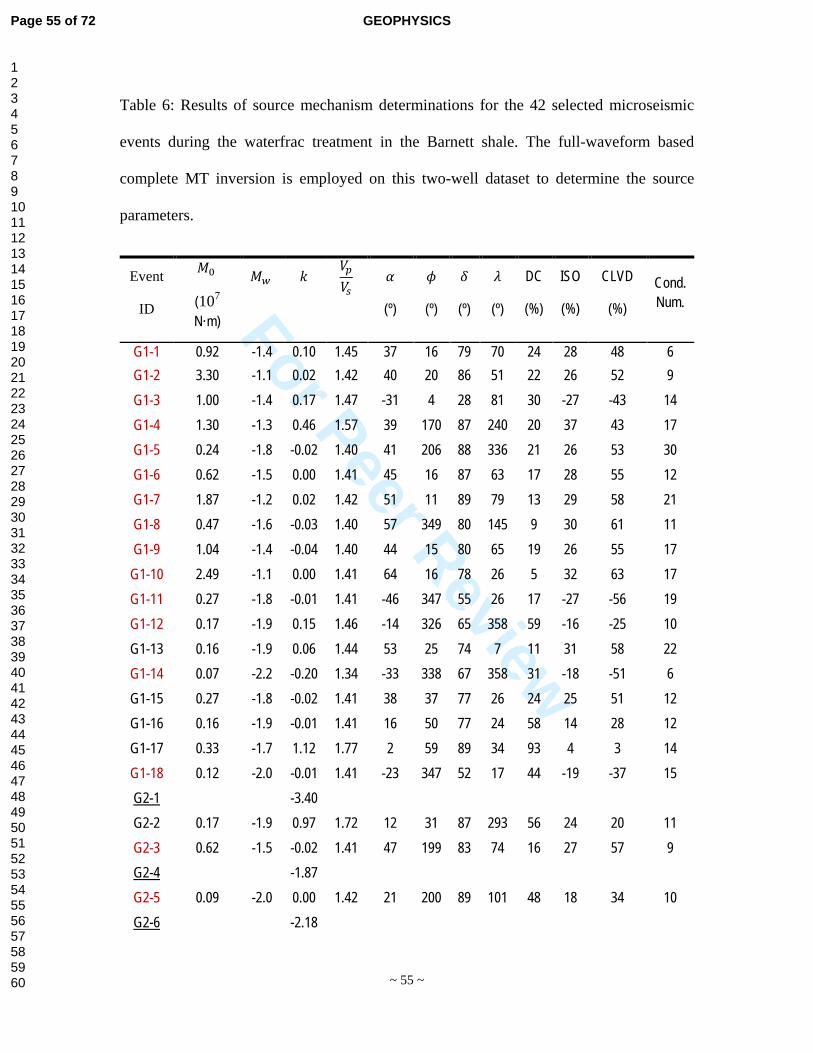
For Peer Review

~ 55 ~

Table 6: Results of source mechanism determinations for the 42 selected microseismic

events during the waterfrac treatment in the Barnett shale. The full-waveform based

complete MT inversion is employed on this two-well dataset to determine the source

parameters.

Event

ID

𝑀0

(107

N·m)

𝑀𝑤

𝑘

𝑉𝑝𝑉𝑠

𝛼

(º)

𝜙

(º)

𝛿

(º)

𝜆

(º)

DC

(%)

ISO

(%)

CLVD

(%)

Cond. Num.

G1-1

0.92 -1.4 0.10 1.45 37 16

79

70

24 28 48 6 G1-2

3.30 -1.1 0.02 1.42 40 20

86

51

22 26 52 9 G1-3

1.00 -1.4 0.17 1.47 -31 4

28

81

30 -27 -43 14 G1-4

1.30 -1.3 0.46 1.57 39 170

87

240

20 37 43 17 G1-5

0.24 -1.8 -0.02 1.40 41 206

88

336

21 26 53 30 G1-6

0.62 -1.5 0.00 1.41 45 16

87

63

17 28 55 12 G1-7

1.87 -1.2 0.02 1.42 51 11

89

79

13 29 58 21 G1-8

0.47 -1.6 -0.03 1.40 57 349

80

145

9 30 61 11 G1-9

1.04 -1.4 -0.04 1.40 44 15

80

65

19 26 55 17 G1-10

2.49 -1.1 0.00 1.41 64 16

78

26

5 32 63 17 G1-11

0.27 -1.8 -0.01 1.41 -46 347

55

26

17 -27 -56 19 G1-12

0.17 -1.9 0.15 1.46 -14 326

65

358

59 -16 -25 10 G1-13

0.16 -1.9 0.06 1.44 53 25

74

7

11 31 58 22 G1-14

0.07 -2.2 -0.20 1.34 -33 338

67

358

31 -18 -51 6 G1-15

0.27 -1.8 -0.02 1.41 38 37

77

26

24 25 51 12 G1-16

0.16 -1.9 -0.01 1.41 16 50

77

24

58 14 28 12 G1-17

0.33 -1.7 1.12 1.77 2 59

89

34

93 4 3 14 G1-18

0.12 -2.0 -0.01 1.41 -23 347

52

17

44 -19 -37 15 G2-1

-3.40

G2-2

0.17 -1.9 0.97 1.72 12 31

87

293

56 24 20 11 G2-3

0.62 -1.5 -0.02 1.41 47 199

83

74

16 27 57 9 G2-4

-1.87

G2-5

0.09 -2.0 0.00 1.42 21 200

89

101

48 18 34 10 G2-6

-2.18


123456789101112131415161718192021222324252627282930313233343536373839404142434445464748495051525354555657585960

For Peer Review

~ 56 ~

G3-1

0.06 -2.2 -0.09 1.38 -21 125

42

156

49 -15 -36 4 G3-2

0.18 -1.9 0.34 1.53 21 64

82

152

43 25 32 8 G3-3

0.07 -2.2 0.28 1.51 -20 286

57

146

46 -22 -32 12 G3-4

-0.81

G3-5

-1.05

G3-6

-2.01

G3-7

0.47 -1.6 0.26 1.50 36 49

88

193

24 45 31 10 G3-8

0.95 -1.4 -0.06 1.39 26 57

89

159

40 19 41 9 G3-9

0.23 -1.8 0.34 1.53 15 228

85

199

54 20 26 11 G3-10

0.92 -1.4 0.08 1.44 32 285

90

19

30 25 45 10 G4-1

1.43 -1.3 -0.05 1.40 -31 334

72

4

32 -22 -46 28 G4-2

0.97 -1.4 0.00 1.41 -57 349

75

7

9 -30 -61 23 G4-3

1.50 -1.3 0.00 1.41 -50 346

74

8

13 -29 -58 28 G4-4

1.08 -1.4 0.04 1.43 38 35

87

27

24 26 50 33 G4-5

0.83 -1.5 0.04 1.43 -40 344

73

5

22 -27 -51 27 G4-6

1.66 -1.3 0.11 1.45 41 208

88

322

20 29 51 33 G4-7

7.26 -0.8 -0.03 1.40 -49 344

71

13

14 -28 -58 34 G4-8

0.52 -1.6 1.37 1.84 2 230

84

156

89 7 4 42

Note 1: The strike, dip, rake, and slope angles follow the convention of Aki & Richards [2002], and are defined in the Figure 1. Note 2: The underlined events are classified as events that can not be modeled by the tensile earthquake model of Vavryčuk [2001]. The highlighted events in red and blue are classified as events associated with reactivation of natural fractures striking along N-S and WNW directions, respectively. The rest of the events in black, except the underlined events, correspond to the events striking along SHmax (NE-SW) directions. Please see the main text for details.


123456789101112131415161718192021222324252627282930313233343536373839404142434445464748495051525354555657585960

For Peer Review

~ 57 ~

Figure 1. A model for the tensile earthquake (after Vavryčuk, 2011; Aki & Richards,

2002). See the main text for the definition of strike ϕ, dip δ, rake λ, and slope angle α.


123456789101112131415161718192021222324252627282930313233343536373839404142434445464748495051525354555657585960

For Peer Review

~ 58 ~

Figure 2. (a) One-dimensional P- and S-wave velocity model derived from the field study

shown in the black. The blue lines on the left and right sides denote the observation wells

1 and 2, respectively. The red triangles represent the depth of the 12 geophones in each

observation well. The rock type for each layer is also listed in the figure. The waterrefrac

treatment is performed in the lower Barnett interval, with the majority of microseismic

events occurring also in the lower Barnett interval. (b) The red and blue lines depict the

perturbed P- and S-wave velocity models to study the influence of velocity model errors

on the inverted source parameters. Please see the main text for details.

2000 2500 3000 3500 4000 4500 5000 5500 6000 6500

2000

2050

2100

2150

2200

2250

2300

2350

2400

2450

Velocity (m/s)

Dep

th (m

)

Lower barnett

Upper barnett

Viola limestone

Forestburg limestone

Barnett lime

Marble Falls limestone

Lower Marble Falls

a)well 1 well 2

Shale

Shale

Vp referenceVs reference

2000 2500 3000 3500 4000 4500 5000 5500 6000 6500

2000

2050

2100

2150

2200

2250

2300

2350

2400

2450

Velocity (m/s)

Dep

th (m

)

b) Vp referenceVs referenceVp perturbedVs perturbed


123456789101112131415161718192021222324252627282930313233343536373839404142434445464748495051525354555657585960

For Peer Review

~ 59 ~

Figure 3. Horizontal plane view of the microseismic event locations from waterfrac

treatment in the Barnett shale plotted as red circles. The yellow and green squares denote

the two vertical observation wells 1 and 2, respectively, while the treatment well

trajectory is plotted as the cyan line with treatment wellhead shown as the blue square.

The origin (0, 0) corresponds to the location of observation well 1. The green dotted line

represents the observation well plane. A total of 42 events located off the observation

well plane with good signal-to-noise ratios are selected for source mechanism study in

this paper. Among the selected events, 4 event groups are seen and denoted as G1, G2,

G3, and G4, respectively.

-350 -150 50 250 450-200

-100

0

100

200

300

400

500

600

700

800

East (m)

Nor

th (m

) G2

G1

G3

G4

Treatment well trajectory

Observation well 1

Observation well 2


123456789101112131415161718192021222324252627282930313233343536373839404142434445464748495051525354555657585960

For Peer Review

~ 60 ~

Figure 4. Moment tensor inversion of a synthetic tensile source located within the event

group G1 (see Figure 2): the normalized variance reduction as a function of searched

event origin time and event location. 10% Gaussian noise is added to the noise-free data

of the synthetic tensile event G1 to form the noisy synthetic data for inversion. The

complete moment tensor inversion is applied to the band-pass filtered horizontal

components from two wells. The inversion is performed with an inaccurate velocity

model and a mislocated source. The variance reduction described in this figure

corresponds to one noise and velocity model realization. The initial event location and

origin time is shown as the black star, while the grid search inverted event location and

origin time is plotted as the white star. Detailed information regarding this synthetic test

is explained in the main text.


123456789101112131415161718192021222324252627282930313233343536373839404142434445464748495051525354555657585960

For Peer Review

~ 61 ~


synthetic data in red for the synthetic tensile source G1. a) North component plot. b) East

component plot. The relative scaling factors between well 1 (geophones 1-12) and well 2

(geophones 13-24) are listed. The modeled data are generated from the inverted

microseismic moment tensor matrix (6 independent elements). The waveform

comparison presented in this figure corresponds to the same inaccurate velocity model

and noise realization as shown in Figure 4. Detailed information regarding this synthetic

test is described in Figure 4 and explained in the main text.

0.02 0.04 0.06 0.08 0.1 0.12 0.14

0

5

10

15

20

25

Geo

phon

e in

dex

Time (seconds)

W2:W1 = 66:100 a)

0.02 0.04 0.06 0.08 0.1 0.12 0.14

0

5

10

15

20

25

Time (seconds)

W2:W1 = 188:100 b)


123456789101112131415161718192021222324252627282930313233343536373839404142434445464748495051525354555657585960

For Peer Review

~ 62 ~

Figure 6. The errors of the inverted event location in (N, E, D) directions for the synthetic

tensile source G1 are shown as stars and plotted as a function of velocity model

realizations. 100 moment tensor inversions, each with one inaccurate velocity model and

noise realization, are performed to study the influence of velocity model errors on the

inverted source parameters. The event location error is shown as multiples of search grid

size. The black line represents the search limit in the vertical direction for the grid search

based moment tensor inversion, while the search limit in the north and east directions is

identical and plotted as the green line. Detailed information regarding this synthetic test is

described in Figure 4 and explained in the main text.

0 20 40 60 80 100-8

-6

-4

-2

0

2

4

6

8

Velocity model realizations

Eve

nt lo

catio

n er

ror (

grid

)

NorthEastDown


123456789101112131415161718192021222324252627282930313233343536373839404142434445464748495051525354555657585960

For Peer Review

~ 63 ~


tensile source G1. 100 moment tensor inversions, each with one inaccurate velocity

model realization, are performed to study the influence of velocity model errors on the

inverted source parameters. Detailed information regarding this synthetic test is described

in Figure 4 and explained in the main text.

-90 -50 -10 30 700

20

40

Cou

nts

Errors in M0 (%)-5 0 5 10

0

50

100

Estimated k-40 0 40 800

20

40

Errors in α (0)

-110 -60 -10 40 900

20

40

Errors in φ (0)

Cou

nts

-20 0 200

10

20

30

Errors in δ (0)-90 -50 -10 30 700

50

100

Errors in λ (0)

-20 0 20 40 600

10

20

Cou

nts

Errors in DC perc. (%)-40 -10 20 500

20

40

Errors in ISO perc. (%)-50 -10 30 70 1100

20

40

Errors in CLVD perc. (%)


123456789101112131415161718192021222324252627282930313233343536373839404142434445464748495051525354555657585960

For Peer Review

~ 64 ~


synthetic data in red for a compressive source located within the event group G4 (see

Figure 2). The rest of the figure description is analogous to Figure 5.

0 0.05 0.1 0.15 0.2 0.25

0

5

10

15

20

25

Geo

phon

e in

dex

Time (seconds)

W2:W1 = 114:100a)

0 0.05 0.1 0.15 0.2 0.25

0

5

10

15

20

25

Time (seconds)

W2:W1 = 67:100b)


123456789101112131415161718192021222324252627282930313233343536373839404142434445464748495051525354555657585960

For Peer Review

~ 65 ~


compressive source G4. The rest of the figure description is analogous to Figure 7.

-80 -40 0 40 800

10

20

Cou

nts

Errors in M0 (%)-3 -2 -1 0 1

0

50

100

Estimated k-30 0 300

10

20

Errors in α (0)

-20 0 20 40 600

10

20

Errors in φ (0)

Cou

nts

-20 -10 0 100

10

20

30

Errors in δ (0)-20 0 20 400

20

40

Errors in λ (0)

-50 -30 -10 10 300

10

20

Cou

nts

Errors in DC perc. (%)-50 -30 -10 100

20

40

Errors in ISO perc. (%)-50 -30 -10 10 300

20

40

Errors in CLVD perc. (%)


123456789101112131415161718192021222324252627282930313233343536373839404142434445464748495051525354555657585960

For Peer Review

~ 66 ~

Figure 10. The horizontal plane view of the three-dimensional (3D) elliptic hydraulic

fracture model and its characteristic neighbourhood regions. The out of the paper

direciton is the vertical (fracture height) direction. Two characteristic neighbourhood

regions: tip region and broadside region, are classfied according to the different features

of stress perturbations induced by the 3D elliptic hydraulic fracture. Please see the text

for details.


123456789101112131415161718192021222324252627282930313233343536373839404142434445464748495051525354555657585960

For Peer Review

~ 67 ~

Figure 11. The calculated stress perturbations due to the 3D elliptic hydraulic fracture

described in Figure 10. a) Stress decay normal to fracture face along centerline of fracture

in the broadside region. b) Stress decay ahead of the length tip along centerline of

fracture in the tip region.

0 50 100 150-1

0

1

2

3

4

Distance normal to fracture (m)

Stre

ss in

duce

d by

frac

ture

(Mpa

)

a)

Lateral HorizontalVerticalNormal Horizontal

0 5 10 15 20 25 30-5

-4

-3

-2

-1

0

1

2

Distance from tip of fracture (m)

Stre

ss in

duce

d by

frac

ture

(Mpa

)

b)

Lateral HorizontalVerticalNormal Horizontal


123456789101112131415161718192021222324252627282930313233343536373839404142434445464748495051525354555657585960

For Peer Review

~ 68 ~

Figure 12. Schematic illustration of the generation of four different failure types using the

Mohr Circle and Griffith failure envelope. According to the relations between shear stress

τ and normal stress σn , the tensile, hybrid tensile, pure shear and compressive shear

failure modes are defined (Modified after Fischer and Guest, 2011).


123456789101112131415161718192021222324252627282930313233343536373839404142434445464748495051525354555657585960

For Peer Review

~ 69 ~

Figure 13. a) Representation of the shear and effective normal stress on an arbitrarily

oriented fracture with the 3D Mohr circle for a typical Barnett shale waterfrac treatment

(treatment parameters are listed in Table 5). The blue circle on the right corresponds to

the ambient pore pressure p0 , while the left circle is associated with the maximum

possible pore pressure case, that is, the pore pressure is increased to the fracturing

pressure pf. The Griffith failure envelope for the intact rock with the inherent cohesion

strength S0 of 20 Mpa is shown as the red curve. b) The 3D Mohr-circle representation of

the tip region. The black, green and cyan crosses denote the principal stresses along the

original unperturbed Shmin (NW-SE), SHmax (NE-SW) and vertical directions,

respectively. In this figure, the hydrofracture induced stress perturbations are considered

and no fracturing fluid leakage occurs in the tip region. The Griffith failure envelope for

weak zones with the inherent cohesion strength S0w of 2 Mpa is plotted as the red curve.

See the main text for detailed discussions.

-20 -10 0 10 20 30 40-40

-30

-20

-10

0

10

20

30

40

Normal stress σn (Mpa)

She

ar s

tress

τ (M

pa)

p0pf

a)

-5 0 5 10 15 20 25-20

-15

-10

-5

0

5

10

15

20


She

ar s

tress

τ (M

pa)

b)

2δ


123456789101112131415161718192021222324252627282930313233343536373839404142434445464748495051525354555657585960

For Peer Review

~ 70 ~

Figure 14. a) The 3D Mohr-circle representation of the broadside region. In this figure,

the hydrofracture induced stress perturbations are considered. Fracturing fluid leakage is

assumed in the broadside region. See the main text for detailed discussions. The red,

green and blue pluses demonstrate the normal and shear stresses on the fracture planes


to WNW, N-S, NW-SE directions). The corresponding dip angles of these fracture planes

are also listed in this Figure. The rest of the figure description is analogous to Figure 13b.

b) Zoomed version of Figure 14a.

-2 0 2 4 6 8 10 12-8

-6

-4

-2

0

2

4

6

8


She

ar s

tress

τ (M

pa)

a)

δ = 800

δ = 450

-2 -1 0 1-1.5

-1

-0.5

0

0.5

1

1.5

2

2.5

3

3.5

4

Normal stress σn (Mpa)S

hear

stre

ss τ

(Mpa

)

b)

δ = 800


123456789101112131415161718192021222324252627282930313233343536373839404142434445464748495051525354555657585960

For Peer Review

~ 71 ~

-0.01 -0.005 0 0.005 0.010

0.1

0.2

0.3

0.4

0.5

0.6

0.7

0.8

0.9

1

Nor

mal

ized

var

ianc

e re

duct

ion

Origin time shift (seconds)

b)

Figure 15. Moment tensor inversion for the field event G1-1. a) The normalized variance

reduction as a function of searched event origin time and event location. The initial event

location and origin time is shown as the black star, while the grid search inverted event

location and origin time is plotted as the white star. b) The normalized variance reduction

as a function of searched event origin time at the optimum event location. The initial and

inverted event origin times are plotted as the black and red stars, respectively.


123456789101112131415161718192021222324252627282930313233343536373839404142434445464748495051525354555657585960

For Peer Review

~ 72 ~

Figure 16. Waveform fitting for field event G1-1. Modeled seismograms derived from

grid search based complete moment tensor inversion are shown in black, while the

observed seismograms are plotted in red. a) North component. b) East component. The

relative scaling factors between well 1 (geophones 1-12) and well 2 (geophones 13-24)

are listed. The inversion is performed on the band-pass filtered horizontal components

and uses the layered model shown in Figure 2a) and Table 1.

0.2 0.25 0.3 0.35

0

5

10

15

20

25

Time (seconds)

W2:W1 = 8.65:1b)

0.2 0.25 0.3 0.35

0

5

10

15

20

25

Time (seconds)

Geo

phon

e in

dex

W2:W1 = 11.65:1a)


123456789101112131415161718192021222324252627282930313233343536373839404142434445464748495051525354555657585960

for peer review - massachusetts institute of technology · for peer review full-waveform based...

Documents