for · inviscid,itwo-dimensional or axisymmetric adiabatic flow of an ideal gas, similarity...

SECOND-ORDER SMALL DISTUEANCE T-IEORY FOR

HYPERSONIC FLOW OVER POWER-LAW BODIES

*H U

n A Dissertation

SPresented to

o 4. .the Faculty of the School of Engineering and Applied Science

o -4U University of Virginia

S-In Partial Fulfillment

.of the Requirements for the Degree

Doctor of Philosophy (Aerospace Engineering)

OLH

!i )

0

- m by

, a I James C. Townsend

Zo

* / December 20, 1974

'"I

&CT)

g3~~~~~9 W £S0r 1 ~I

https://ntrs.nasa.gov/search.jsp?R=19750006923 2020-07-02T01:36:00+00:00Z

APPROVAL SHEET

This dissertation is submitted in partial fulfillment of

the requirements for the degree of

Doctor of Philosophy (Aerospace Engineering)

uthor

Approved:

Faculty Advisor

Dean, School of Engineeringand Applied Science

(Date)

ABSTHACT

Beginning with the equations for conservation of mass,

conservation of momentum, and conservation of energy for the

inviscid,itwo-dimensional or axisymmetric adiabatic flow of

an ideal gas, similarity solutions have been found which give

the flow field to order-6 2 about power-law bodies in the

hypersonic limit M O -, where 6 is a body slenderness

parameter. Some years ago, the hypersonic small disturbance

equations were used to obtain "zeroth-order" similarity

solutions for flow over power-law bodies. The second-order

solutions, which reflect the effects of the second-order

terms in the equations, are obtained by applying the method

of small perturbations in terms of the body slenderness par-

ameter 6 to these zeroth-order solutions. The method is

applied by writing each flow variable as the sum of a

zeroth-order and a perturbation function, each multiplied by

the axial variable raised to a power. When these expanded

variables are substituted into the flow equations, a

zeroth-order set and a perturbation set of four first-order

ordinary differential equations is obtained, and the axial

variation drops out. These equations are integrated

numerically from the shock, where the boundary conditions are

known from the Rankine-Hugoniot relations, toward the body.

The order-62 solutions which are obtained are independ-

ent of the slenderness parameter 6 and thus are universal

in that they apply for all values of 6 for which 6 4 << 1.

However, except when the body power-law exponent is equal to

unity, the velocity functions, which form part of the solu-

tion, have singularities at the body surface. These

singularities are an effect of the entropy layer caused by

the nose bluntness. Since the singularities are not removed

by any of several methods tried, the solutions can only be

applied away from the body surface. (It is suggested for

future work that the singularities probably could be removed

by applying the method of matched asymptotic expansions.)

In comparisons with,the exact solutions for inviscid

flow over wedges and circular cones, the or.der-6 2 similarity

results give excellent agreement for 6 less than about 0.4,

corresponding to wedge or cone angles up to about 200. Over

an even larger range, the order-62 surface pressure predic-

tions are superior to the Newtonian pressure law. The

order-62 results are a significant improvement over the

zeroth-order results for body angles greater than about 120.

In comparisons with experimental shock wave shapes and sur-

face pressure distributions for 3/4-power axisymmetric

bodies, the order-62 similarity solutions.give good results,

considering that Mach number and boundary layer displacement

effects are not included in the theory. For body fineness

ratios near two, the effects of the order-62 terms are

significant only very near the body nose, whereas for a

fineness ratio near unity the order-6 2 terms has a large

effect over al.most the entire body.

The order-6 2 similarity solutions are developed for

infinite Mach number, but the derivation shows that they are

compatible with shock-strength perturbation solutions,

which introduce Mach number effects. Also, while all results

obtained are for no flow through the body surface (as a

boundary condition), the derivation indicates that small

amounts of blowing or suction through the wall could be

easily accomodated.. Finally, it is noted that a correlation

suggested by Hornung for the shock wave shape and body

pressure distribution can be applied exactly to all of the

flow variables in the order-62 similarity solution form.

This finding suggests for future work a possible refinement

of the present derivation, using the local body or shock

wave slope as the small parameter.

ACKNOWLEDG METS

The author wishes to thank Dr. Wesley L. Harris, Sr.,

for serving as principle dissertation advisor, Dr. John E.

Scott, Jr., for serving as committee chairman, and the

remainder of the committee for reviewing this dissertation.

The author is indebted to the National Aeronautics and

Space Administration for permitting the use material ob-

tained as a research project at the Langley Research Center

in this dissertation. He is also indebted to Mr. John T.

Bowen and Dr. Carl M. Andersen for checking much of the

transformations of equations using MACSYMA, a computer

language for algebraic manipulation implemented by the

Math lab group at MIT (supported by ARPA, Dept. of Defense,

Office of Naval Research Contract #N00014-70-A-0362-0001).

Finally, the author thanks his wife, Judy, and his child-

ren for their encouragement and understanding over the long

time period required to complete this work,

TABLE OF CONTENTS

CHAPTER PAGE

ACKNOWLEDGEMENTS . . . . . . . . . . . . . . .

TABLE OF CONTENTS . . . . . . . . .. . . . . . ii

LIST OF FIGURES . . . . . . . . . . . . .. . . . v

LIST OF SYMBOLS. . .. . . . . . . . . . . . ..viii

I. INTRODUCTION . . . . . . . . . . . . . . . . . . 1

II. THEORY . . . . . . . . . . . . . . . . . .. .8

Transformation of Basic Flow Equations . . . . 8

Normalization . . . . . . . . . . . . . . . 8

Similarity variables .. . . . . . . . . . . 10

Equation in .similarity variables . . . . . . 16

Discussion of Orders of Magnitude. . . . . . . 19

Zeroth-order equations . . . . . . . . . . . 19

Order-c equations. . . . . . . . . . . . . . 20

Order-62 equations . . . . . . . . . . . . . 25

Boundary Conditions... . . 27

Shock wave ................. . 27

Body surface . . . . . . . .. . . . . . . . 29

Initial magnitude checks . . . . . . . . . . 32

Momentum Variable Formulation ....... . . . . 34

Normalization . . . . . . . . . . . . . . . 35

Similarity variables . . . . . . . . . . . 36

Zeroth-order equations . . . . ... . . . . . 40

ii

CHAPTER PAGE

Order-6 2 equations ... ..... . . .. . 42

Boundary conditions. . ...... . . . . . 43

Correlation of Solutions . . . . . . . . . . . 46

III. SOLUTION OF EQUATIONS . ... . ..... . .. . 50

General Scheme of Solution . . . . . . . . . . 50

Extrapolation of Order-6 2 Functions. ... .. . 55

Methods for Determining the Constant a2 . 5 5

Iteration method . . . . . . . . . . . . . . 59

Decomposition method .. . ... . ... .. . 59

Description of the Numerical Method. . ..... . 63

IV. DISCUSSION OF RESULTS ...... . ......... . .65

Zeroth-Order Functions . . . . . . . . ... ..;65

Shock Displacement Constant . . . . . . . . .. 74

Order-6 2 Functions . . . . . . . . . . . ... 82

Region of Validity of the Solutions. . .. . 102

Comparison with Other Solutions . .... ... . 104

Comparison with Experimental Results ..... 120

Shock shape . . . . . . . . . . . . . . . . 1121

Pressure distribution. . ....... . . . . . 124

V. CONCLUSIONS. .. ..... . . . . . . . . . . . . . 128

BIBLIOGRAPHY. . .................. . . 131

APPENDIX. ASYMPTOTIC SOLUTION IN TERMS OF STREAM

FUNCTIONS . . . . . . . . . . . . . . . . . . . . . . 134

Stream Function Formulation. .. .... . . . . 134

iv

CHAPTER PAGE

Zeroth-Order Approximate Solution. . ..... . 139

Order-62 Functions . . . .......... 142

IA

LIST OF FIGURES

FIGURE PAGE

1. Power-law and Zeroth-order Shock inPhysical and Transformed CoordinateSystems . . . . . . . . . . . . . . . . . . . . 13

(a) Physical coordinate system. . . . . . . . . 13(b) Normalized coordinate system. . . . . . . . 13

(c) Similarity coordinate system . .. ..... 13

2. Relation Between Body Slenderness Parameterand Shock Strength Parameter for SeveralMach Numbers. . . . . . . . . . . . . . . . . . 21

(a) Relative errors from neglecting termsof order e and of order 62 . . . . . . . 21

(b) Relative errors from neglecting termsof order e2 and of order 62 ....... . 22

(c) Relative er ors from.neglecti g termsof order e and of order 6 . . . . . . . 23

3. Vector Diagram of the Flow at the BodySurface . . . . . . . . . . . . .. . ..... 30

4. Zeroth-order Similarity Functions forTwo-Dimensional flow (a = 0). . . . . . . . . . 66

(a) Pressure function, F (n) . . . . . . . . . 66(b) Density function, o ) . . . .... ... ' 67(c) Longitudinal velocity function, v (n) . . . 68(d) Lateral velocity function, 00(n) . ..... . 69

5. Zeroth-order Similarity Functions forAxisymmetric Flow (o = 1) . . . . . . . . . . 70

(a) Pressure function, F (n). .......... 70(b) Density function, ?n) . . . . . . 71(c) Longitudinal veloci~y function, Vo(n) . . . 72(d) Lateral velocity function, (n). . . . . . 73

6. Zeroth-Order Lateral Momentum Function, %o(n) . 75

(a) Two-dimensional flow (a = 0). . . . . . . . 75(b) Axisymmetric flow (a 1) . . . . . . . . . 76

v

vi

FIGURE PAGE

7. Variation of Shock Displacement Constant a2with Body Power-Law Exponent m . . . . .78

(a) Computed values for a2 . . . . . . . . .. . . . 78(b) Numerator and denominator of expression

for a2 (equation (51)) . . . . . ., . .79

8. Order-6 2 Similarity Functions from theMomentum-Variable Formulation for AxisymmetricFlow (a = 1). . . . . . . . . ... . .......... 83

(a) Pressure function, F (n).... . 83(b) Density function, 2 n) .... ... * . 84(c) Longitudinal momentum function, U 2 (TI) .85(d) Lateral momentum function, P2 (n). .. . .86

9. Order-62 Similarity Functions from theVelocity-Variable Formulation forAxisymmetric Flow (a = 1) ......... ... .87

(a) Pressure function, F (n) . .. . ...... 87(b) Density function, 2 n) . . . . 88

(c) Longitudinal velocity function, v2(n) . . .89(d) Lateral velocity function, P2 (n) . . . ....90

10. Order-6 2 Similarity Functions from theVelocity-Variable Formulation for Two-Dimensional Flow (a = 0). . .......... .92

(a) Pressure function, F (n) . . . . . . . . .92(b) Density function, 2 n) . . . . . . . . .93(c) Longitudinal velocity function, v2 (n) . . .94(d) Lateral velocity function, p2 (n) ..... . 95

11. Order-62 Similarity Functions from theMomentum-Variable Formulation for Two-Dimensional Flow (a = 0). . .......... .96

(a) Pressure function, F2 (n). . . . . . . . . .96(b) Density function, 2Tn) . . . . .. . . .97(c) Longitudinal momentum function, p2(n) . . .98(d) Lateral momentum function, P2 (n) ...... 99

vii

FIGURE PAGE

12. Comparison of Similarity Solution form = 1 with Exact Solution for FlowOver a Wedge at M, = . . .... ...... 105

(a) Shock wave angle, . . . . . . . . . . . 105(b) Pressure, /q. . . ........... 106(c) Magnitude and direction of the

velocity vector . ..... ...... . . 107(d) Velocity components . . . . . . .... . 108

13. Comparison of Similarity Solution for m = 1with Exact Solutions for Flow Over aCircular Cone at Me = . . . . . . . . ... . 109

(a) Shock wave angle. ............ . . 109(b) Surface pressure, pb/ . . . . . . . 110(c) Magnitude and direction of the velocity

vector at the body surface . . . . . . . 111(d) Surface velocity components . ..... . 112

14. Variation of Flow Variables from Body to-Shock at x/ = 0.5 for Axisymmetric .Flowwith 6 = 0.4 . . . ... . . . . . . . . . . 116

(a) Power-law exponent m = 1.0(conical body). . . . . . . . . . . . . . 116

(b) Power-law exponent m = 0.85. . . . . . . 117(c) Power-law exponent m = 0.75. . . . . . . 118

15. Shock wave shape correlation for axisym-metric 3/4-power bodies . ......... .122

16. Comparison of Similarity Solutions withExperimental Pressure Distributions forAxisymmetric 3/4-power Bodies . . . . . ..... 125

LIST OF SYMBOLS

al, a2 shock wave displacement constants (equation (7))

B constant in similarity form of stream function

(equation (A2))

C pressure coefficient,

D constant in stream function solution of longitudinal

velocity variable (equation (A15))

f body fineness ratio, lengthmaximum thickness

F similarity pressure function

J exponent in stream function expression (equation

(A2))

, body length

m power law exponent

M. free stream Mach number

p pressure

1 - -2q, free stream dynamic pressure, 2 p uC

r lateral coordinate

R lateral coordinate of shock wave

u longitudinal velocity

v lateral velocity

vw flow velocity through body surface (normal to wall)

x longitudinal coordinate

Pwa density ratio at wall, -'

PbB alternate shock shape parameter, 2(1-m)

(l+o)m

viii

ix

y ratio of specific heatsRo(g)

6 slenderness parameter, 0

E shock wave strength parameter, (6M) - 2

n similarity lateral coordinate

Gb body surface angle

Os shock wave angle

e similarity stream function

similarity lateral momentum function

v similarity longitudinal velocity function

Ssimilarity longitudinal coordinate

p density

a 0 for planar flow, 1 for axisymmetric flow

u similarity longitudinal momentum function

similarity lateral velocity function

w similarity velocity through body surface

similarity density function

P 'stream function

w entropy function, p/pY

Subscripts:

a part of decomposed function multiplied by a2

(equation (48))

b body surface

c part of decomposed function independent of a2

(equation (48))

s shock wave

w flow through the wall

0 zeroth order

1 order e

2 order 62

free stream

A prime denotes the derivative of a function of one variable.

A bar over a variable denotes that it has physical dimen-

sions. A tilda over a dependent variable denotes that it is

a function of the normalized lateral coordinate r rather

than the similarity lateral coordinate n.

CHAPTER I. INTRODUCTION

A great deal of research has gone into investigating

solutions to the small disturbance equations for hypersonic

flow. One area that has received particular attention is

that of self-similar solutions for power-law profile bodies.

While the effects of shock wave strength have been investi-

gated in connection with these solutions, there apparently

have been no reported efforts to investigate the effects of

neglecting the second-order terms of the complete inviscid

flow equations in order to reduce them t-o the small distur-

bance form. The purpose of the present study is to determine

the effects of retaining these terms by using.a perturbation

analysis to obtain second-order similarity solutions for

power-law bodies.

Since this dissertation will be concerned with finding

a particular set of similarity solutions of the inviscid

flow equations, it is important at the outset to establish

what is meant by similarity solutions in hypersonic flow.

The similar solutions referred to here are solutions for

self-similar flows; i.e. flows for which the flow field

(expressed in suitable coordinates) at any one position

along the body is the same as that at every other position.

(In the corresponding unsteady self-similar flows, the flow

field in suitable coordinates at any one time is the same as

that at every other time.) Inviscid axisymmetric supersonic

1

2

flow over a cone with an attached shock wave is a classical

example of a self-similar flow and represents a particular

case of the similar solutions discussed herein. For the

cone, the flow field properties (eg. the pressure, the density,

and the velocity components) are themselves constant along

rays from the cone vertex. For the other power-law bodies,

the flow field properties are not constant themselves, but

similarity functions describing these properties are

constant (to the order of the solution) along curved power-

law paths from the nose of the body.

The similar solution approach to solving the flow

equations is valuable because it allows a reduction in the

number of independent variables in the problem, In particular,

for hypersonic flow about power-law bodies, the similarity

approach reduces a system of partial differential equations

to a system of ordinary differential equations. As noted by

Hayes and Probstein (1), generally these flows occur only

for a self-similar fluid (the most practical example of which

is a perfect gas with a constant ratio of specific heats)

and a self-similar shock wave, i.e. one having the same

density ratio across it at every position.

All of the early investigations of similar solutions

related to the present problem were concerned with unsteady

flows. Early in the Second World War, Taylor (2) developed

a similar solution for the flow behind the spherical shock

wave produced by the instantaneous release of energy at a

point (e.g., an atomic explosion). Sakurai (3,4) generalized

Taylor's approach to obtain solutions for cylindrical and

planar shocks as well. He also introduced perturbation

analysis as a means of obtaining solutions for more moderate

shock wave strengths. The equivalence of these unsteady flows

to steady flows in one additional space dimension was pointed

out by Hayes (5). This equivalence applies to the inviscid

flow equations reduced to the hypersonic small disturbance

form, as derived by Van Dyke (6).

Lees (7) found that there are self-similar flow fields

for bodies having power-law profiles, and Lees and Kubota

(8) determined the range of power-law exponents for which

the similarity holds. Kubota (9) obtained numerical solutions

for this case (herein called the "zeroth-order" case)-; he

also applied a perturbation in the strong shock parameter (as

Sakurai had done for unsteady flow) and numerically obtained

first-order similar solutions for moderately strong shock

waves. Mirels (10) computed additional and more accurate

numerical results for the zeroth-order and moderately-strong

shock wave cases. He also derived approximate analytical

solutions for these cases.

The parallel but independent work of investigators in

the USSR has been thoroughly described by Hayes and

Probstein (1). Beginning at about the same time as Taylor,

Sedov (11) studied the intense spherical explosion problem

in a more general form and developed an analytic solution

for it (12). Grodzovskii (13) and Chernyi (14) applied the

unsteady results to the steady hypersonic flow problem.

Stanyukovich (15) and others investigated a number of

related problems.

All of the important developments in the use of hyper-

sonic small disturbance theory to obtain solutions for power-

law bodies were treated in a unified way by Mirels (16), who

added an analysis of perturbed power-law body shapes. More

recently, Freeman (17) investigated the effects of the entropy

layer caused by the nose bluntness of the power-law bodies

and determined the power-law exponents below which the

entropy-layer effects predominate. Again independently,

Sychev (18) developed a correction to the power-law body

shape to account for the effect of the entropy layer.

A few experimental investigations of the flow field over

power-law bodies have been made. Kubota (9) compared his

theoretical results to surface pressure distribution and

shock wave shapes measurements for 2/3- and 3/4-power bodies,

obtaining good agreement for the more slender bodies.

Peckham (19) measured pressure distributions and shock wave

shapes for a series of power-law bodies, some of which fall

in the similar-solution range. Freeman, Cash and Bedder (20)

and Beavers (21) also presented detailed shock shape data

for series of power-law bodies, registering some disagreement

with Kubota's results. Spencer and Fox (22) present aero-

dynamic drag and other data for several power-law bodies

over a wide Mach number range. Ashby (27) presents aero-

dynamic data for a similar series of bodies over a range of

Reynolds numbers at Mach 6, and Ashby and Harris (28) use

method of characteristics and boundary layer computer pro-

grams to show the important effect of boundary layer transi-

tion on the total drag of those bodies.

Townsend (23) applied the zeroth-order solution of

Kubota and Mirels, with their shock-strength parameter per-

turbation and a boundary layer displacement correction, to

the problem of estimating the forces and moments on a half-

axisymmetric body under a thin, flat wing. In order to study

a range of configurations at a moderately hypersonic Mach

number, Townsend applied his method to configurations which

are marginally slender, (i.e. to configurations for which

the errors arising from body thickness are small but not

negligible). This type of application points up two

reasons for seeking solutions which include the effects

of the second-order terms for body slenderness in the flow

equations: (1) to assess the error caused by making the

small disturbance assumption, and (2) to improve the

accuracy of calculations for marginally slender bodies.

When compared with experimental data for axisymmetric

power-law bodies and for wing - conical-body configurations,

Townsend's method gave good agreement where the basic

assumptions were satisfied. An example series of computations

with variations in the principal parameters at a full-scale

flight condition showed that varying the power-law exponent

has a greater effect on longitudinal stability and trim than

on the lift-drag ratio. The computations for Mach 6 gave

higher maximum lift-drag ratios, higher drag coefficients at

zero lift, but essentially the same stability characteristics

as their counterparts for Mach 12.

In the present study the second-order similarity solu-

tions were obtained by a perturbation method. This method

used expansions of the variables in terms of a small parameter

to obtain higher-order solutions as perturbations from a

known zeroth-order solution. The approach was very similar

to that of Sakurai (4), Kubota (9), and Mirels (16) in their

first-order determinations of the effects of shock wave

strength; but, the small parameter used herein was a body

slenderness parameter rather than the shock strength parameter.

Van Dyke (29) describes the application of perturbation

methods to fluid mechanics, and Van Dyke (30) shows how, in

favorable cases, such solutions can be extended to improve

convergence when the perturbation quantity is not small.

The importance of the results to be obtained from the

present study lies in their practical application. The

principle area for this is in estimating the aerodynamic

characteristics of generalized configurations (e.g.,

Townsend's (23) family of wing-body combinations). By

improving the results of such studies and by better defining

their limits of applicability, the present work contributes

to their usefulness in suggesting designs (or parts of

designs) for such hypersonic vehicles as transports or re-

entry spacecraft.

The remainder of this dissertation will describe the

development of the solutions and present the results.

Chapter II gives the theoretical development. It goes

through the transformations of the flow equations required

to put them into similarity form, discusses the results of

keeping terms of different order, describes the application

of the boundary conditions, and develops an alternative

formulation of the problem. Chapter III presents the general

scheme for solving the equations and deal.s with the diffi-

culties which arise. Chapter IV discusses the results and

their region of validity. Chapter V gives the conclusions

reached as a result of this study. The Appendix describes

an approximate analytical solution used near the body sur-

face, where the equations are singular.

CHAPTER II. THEORY

A. Transformation of Basic Flow Equations

This section will show how the basic flow equations can

be transformed to obtain a separation of variables for the

case of'hypersonic flow over power-law bodies. The starting

point for this process is the system of steady, two-dimen-

sional, inviscid flow equations for a perfect gas in physical

variables:

Continuity: pu pv + pv 0-- + r + 0x r

au -u 1 apLongitudinal u - + + 0ax aF p -xmomentum: x

.(1)

Lateral u + v + = 1 = 0ax VF p armomentum:. p

Energy: + 0=

The constant a in the continuity equation has the value

0 for planar flow (Cartesian coordinates) or the value 1

for axisymmetric flow (cylindrical coordinates). The bars

over the variables indicate that they are dimensional

quantitites.

Normalization. The initial treatment of these equations

follows that of Kubota (9) (also covered by Mirels (16)),

8

except that no terms are dropped. Kubota showed that for

slender bodies in hypersonic flow the variables can be norma-

lized using the expressions:

x r= r6£ ' 2- -2

6 PU (2)

u-u 0 0 -Vp c vp 2- 6

The 6 is a body slenderness parameter (to be discussed

later) introduced so as to make the dimensionless variables

of order unity. These variables are substituted into equa-

tions (1) to obtain the normalized flow equations:

Continuity: 62 + -- + + 0ax ax 3r r

2 u Du au 1 DpLongitudinal 6 u + -+ v U+ a 0

mx ax ar p axmomentum:

(3)

2 av av av 1 pLateral 62 u + + v - + - = 0momentum: pr

Energy: 62u - + +

Note that each of these equations contains a leading term in

62. If the body were sufficiently slender, the order-6 2 terms

could be dropped, leaving the hypersonic small disturbance

equations used by other workers. For the present study,

however, the equations are retained in the complete form.

10

Similarity variables. The next step is to put the flow

variables into similarity forms. Still following Kubota (9),

these will be found by comparison with the flow through an

oblique shock wave. The normalized flow variables just

behind an oblique shock are (24):

PS 1 sSs 2- -2 2 2 p

6 pW U 6y Y o

2yM sin 2 - (Y-1)1C s

Y62M2 y + 1

p (y+l)M 2 sin2 0

P (-m 2 sin 20 +2Cu s

2- 2 2

6 (y1)M sin (Y+l)M

S[2 1 -(M sin - 1)1s 62 2 u 2 2

CO (y+l) m(

If the shock wave shape is given by R(x), its slope is

R'(x) '-dR = 6 dR 6R'. The shock wave angle 's is

related to slope by tan Os = ' = 6R', from which

sin 2 O 62R2 Putting these results into the oblique1 + 6 2 I2

shock relations gives (for R' of order unity):

= t2 _

S+l 2 2 y

R y+l R' 4a)

pR262l y-l 0(6) (4a)Y+l y+1 y+1 y

2R 1s y-li + y-1 R' 2

(4b)

y+l _ 2(y+l) 4 + 0(64)

y-1 (y-1)2 R'2

2 R'y+l 1 1+62R' 2

2 R2 + 2 62R 4 + 2 0(4 (4c)- R' + -2 6R + + 0(6 )

y+l y+l y+1

2 R' ss y+l 1 + 62R '2

(4d)

2 R' 2 62 R' 3 2 e + 0(61y+l y+1 y+l R'

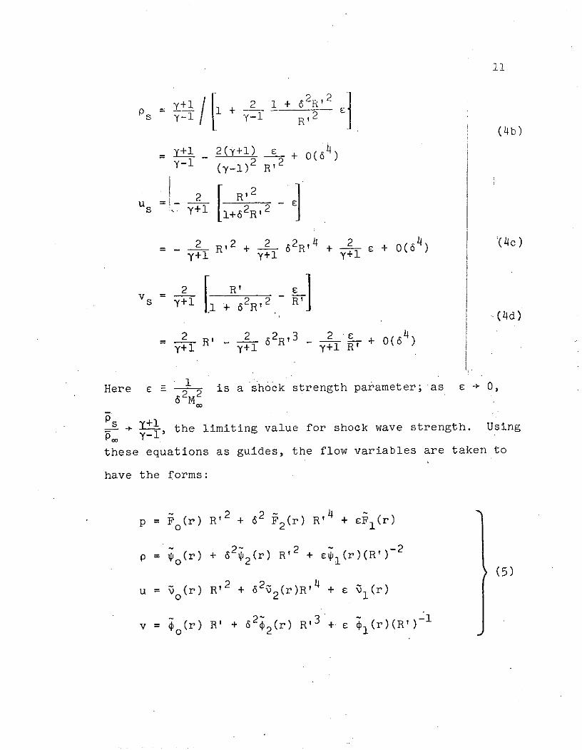
Here c _ 2 is a shock strength parameter; as SE 0,62M 2

s y+l the limiting value for shock wave strength. Usingp0 y-l'

these equations as guides, the flow variables are taken to

have the forms:

22 4p = Fo(r) R '2 + 62 F2 (r) R

' + eF 1 (r)

6 2' -2p = 0o(r) + 62 2(r) R ' 2 + e (r)(R')-2

(5)

u = vo(r) R' 2 + 62Z 2 (r)R'4 + E v1 (r)

(r) R' + 2 2(r) R' 3 + (r)(R)-1v = (r R' + 6 ,(r) R' + e 4,r(R' )

12

At this point, in order to get an expression for the

shock wave shape, consideration is narrowed to flows about

power-law bodies. Under the hypersonic small disturbance

- -massumptions, a power-law body (rb ~ xm) produces a power-lawIm2

shock wave (R ~ xm) for 2 < m < 1. (See Lees and Kubota3+0

(8).) Specifically, for 62 << 1 and e << 1, the "zeroth-

6rder" shock shape about a body b 2 = is given byR _ m

- = 6 ; or,.in normalized coordinates, the shock shape

about a body r = 1 x is R xm (Figure 1, partsb 26f o

(a) and (b)).. Note that for m=l the body is a wedge'(for a = 0)

or a cone (for a = 1), both of which are known to have straight

shock waves and therefore satisfy the above relations. For

m iif1, the power-law body has a small blunt nose, so that the

shock wave is detached. Consequently, this type of relation

between the body and the shock cannot hold in the immediate

vicinity of the nose. The effects of nose bluntness on the

flow downstream are confined to a thin layer near the body

surface. 'Freeman (17) found that the effects are less than

-2 2 (-y+1)order M 2 for m > (+u)+2 (For Y = 7/5 this amounts

24 24to 31 .77 for a = 0 and to 3- z .63 for a = 1).

The expression for the zeroth-order shock wave shape

serves to define the slenderness parameter 6. That is,

o(x) = 6 () evaluated at x = £ gives the relation

Ro(Te6 = .Thus, 6 is the tangent of an angle defined by

13 -

2-

2f Shock, Ro= 8,

Ston-'80

Longitudinal distonce,l

Body, b =

8f x

0

-j

0 1

Longitudinal coordinate, x

(b) Normalized coordinate system.

Shock, 7)=I

Body 7 = 7bIb

C

000

0

Longitudinal coordinate,

(c) Similarity coordinate system.

Figure 1. Power-law and Zero-order Shock in Physical and.............. Transformed Coordinate Systems.

the shock wave position (Figure l(a.)) and is, in fact, a

"mean shock wave angle" parameter. However, since the

zeroth-order case implies Mo + M (as will be seen), the

shock lies near the body so that the shock wave angle and

body slenderness are closely related. The definition of 6

is made in terms of the shock for convenience, since the

solutions are to be found by integrating from the shock to

the body.

To aid in the separation of variables, a shock-oriented

coordinate system is now introduced (Figure l(c)). This

system has

S = x and n = (6)R

0

so that r = Ro = nx = ngm . The body surface is then

rb = Tb)' where ob 26f'

The shock wave shape to be used in equations (5) is the

zeroth-order shock with Kubota's (9) shock strength pertur-

bation and a separate perturbation for the body slenderness.

It is taken to be

R(x) = R (1 + 62a2R2 + ealm2R-2

where the constants al and a2 are to be determined as

part of the solution. (The factor m 2 is included in the

15

last term of this equatioh so that it conforms to the usage

of Kubota and Mirels.) Putting in R = m

mR 2 2 -2 (1-m ) 2 (1-m ) (7)R(C) C + 6 a2 Cm (+ea5 l

Substituting the derivative of equation (7) into equa-

tions (5) and ordering the terms by powers of 6 and E

give expressions for the flow variables in the following form

(neglecting terms of order 64 and of order 2:

p(,n) = ()m 2 -2(1-m) 2 4 -4(1-m)+() IF (n)m .+ 6 F (n)m

2. +sEF l ()m

,n) = (n) + 622( 2 -2(1-m) + 2(1-m)p(o() Wrn + 6(l E(O (fl) C

(8)

u(S,n) = vo(n)m2 -2(1-m) + 62 (n)m4 -4(1-m)

+ V1 (+)m2

S (,) m (1-m) 2 () 3 -3(1-m)v(C~) = 50(n)m 5+ 6 Wm

+ l() (1-m)

The relations between the functions of n and the functions

of r in equations (5) are not needed since it is easier to

d16

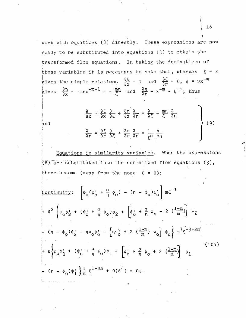
work with equations (8) directly. These expressions are now

ready to be substituted into equations (3) to obtain the

transformed flow equations. In taking the derivatives of

these variables it is necessary to note that, whereas ( = x

! 8 -mgives the simple relations - 1 and -0, - = rxi theax ar

. n r-m-1 mn a n -m -mgives 3n -mrx - and x = ; thus

x 3 r

a a a 3 a mn aax ax a ax an a~ an

and (9)

a aa a a 1 a+ -ar r 9 r arn m aarn

Equations in similarity variables. When the expressions

(8-) are substituted into the normalized flow equations (3),

these become (away from the nose ( = 0):

a1continuity: ) - (n - m

62 + 2 o o - 2 ( m 2

- (n - o - ~o - + 2 (1-) V ] o m3E-3+2m

+ + ( + + + o + 2 ( 1a)

(n - o)1 } 1-2m + 0(6) = 0;

17

Longitudinal momentum:

1 ' F

i - + o) - 2( - -)(vo

2 (T v + rF + 4(F + m 2F' F

0 m

mo2 o m o

S -}m I + nO(4) -= 0;

Lateral momentum:

(o (l-)~ m 2 -2+m

2 2 2 ) 2

o 'o (10c)

S + (-) v m4+3m

1 o - +-m -m

+ (1 2 m 1

+ 0(64 ) = 0;

18

10F F _ (mEnergy: - )(Y o) - 2( M

S2 F!2 F2 2 o F2 F'o+ 6 (n- ¢o -F2 2

F o F Fim 22 (2 o o

+ 2( ) (y ) - (Ym J F F20 0 0 0

0 Fj ')]v 33+ (10d)2 - ) - 2(y m

I F 1 o F2]

m FF21lI( 1 1 o 0(64 0.

.These equations are seen to be ordinary first-order differen-

tial equations, linear in the derivatives of the functions

defining the pressure, density, and velocity fields. It is

noteworthy that although 6 appears to the first power in

the normalization of variables (equations (2)), only the even

powers of 6 appear in the final form of the flow equations.

Thus, while the solutions to be found are of second order

in the body slenderness parameter 6, they could be considered

of first order in 62. To avoid any ambiguity they will

generally be referred to as order-62 solutions. Physically,

the absence of lower powers of 6 indicates that the error

due to a given body thickness is less at hypersonic speeds

than at lower speeds,where terms of order 6 or 63 / 2 appear

(Van Dyke (6)).

19

B. Discussion of Orders of Magnitude

As a result of the normalization procedure (equation (2)),

the variables p, p, u, and v are of order unity for slender

bodies in hypersonic flow. The similarity variables in

!quations (10) are also considered to be of order unity, but

this assumption must be tested by the results obtained. The

development so far has been based on 62 and e being small

parameters. This section will consider their relative

sizes.

Zeroth-order equations. If 62 << 1 and << 1, so

that all terms containing either one may be neglected,

equations (10) are reduced to the zeroth-order equations:

Continuiy: ( , + )

Longitudinal (n - 0 )v' + o + 2(m )(v) = 0momentum: o o m

F' (11)Lateral momentum: (n - ) , o + (1m)o = 0

o Ft m oEnergy: (N - 2)(Y ( o1-

These equations represent the case first studied by Kubota

(9); they are the same as his equations except that he

omitted the longitudinal momentum equation, which is

uncoupled from the others. References 9, 10, and 23 contain

results of numerically solving Kubota's equations, which are

a special case of the present more general treatment.

20

Equations (11) contain only one parameter, the power-law

exponent m. Thus, for two-dimensional flow (a = 0) or

axisymmetric flow (a = 1) of a given gas, the similar solu-

tions F(n) , 9o(n), vo(n), and 0o(r) each form two

families of "universal functions" depending only on the

power-law of the body.

As was mentioned in Chapter I, the simultaneous applica-

tion of the conditions leading to these equations imposes a

stringent condition on the Mach number; viz., 62 << 1 and

c 2 << 1 requires M >> 1. This relation between cM26

and 6 is illustrated in Figure 2-, where part (a) shows,

for example, that s < .1 and 62 < .1 are both true at

Mach 12 only if 6 .3. Note, in addition, that dropping

the terms in s removes all Mach number dependence from the

equations, which really implies M. + and illustrates

Hayes' "Mach number independence principle" (ref. 1).

Order-c equations. If, in equations (10), the terms in

62 << 1 are dropped but the terms in c are retained, two

systems of equations can be obtained by setting the zeroth-

order and order-c terms separately equal to zero. The

zeroth-order system is the same as before; the order-s

system is:

Continuity:

So)1 (n - o) + [ o + + m =0 0o + 2( 0 -0 mO

(12a)

.7

N.= 24.0 12.0 6.0 3.0 --.15---

H

W.4I-

(0

-E= 0.05

0 -J0.02

O .1 .2 .3 .4 .5 .6 .7 .8 .9 1.0

BODY SLENDERNESS PARAMETER, 8

(a) Relative errors from neglecting terms of order E and of order 62.

Figure 2. Relation Between Body Slenderness Parameter and Shock Strength Parameterfor Several Mach Numbers.

= 24 .0 6.0 3.0 1.5

u.5I'-

E:=0.2

Q .4II-

2 2

282_0.1

E :0.02

. .01 ?)- 0 g2a :0.05

1 .0 18 202

0 .Q50 .1 .2 .3 .4 .5 .6 .7 .8 .9 1.0

BODY SLENDERNESS PARAMETER,8

(b) Relative errors from neglecting terms of order e2 and of order 62.

Figure 2. Continued.

.7

M =24.0 12.0 6.0. 3.0 . - 5-

L .5

I-

S.2-

I

0.2

0 .1 .2 .3 .4 .5 .6 .7 .8 .9 1.0

BODY SLENDERNESS PARAMETER, 8

(c) Relative errors from neglecting terms of order c2 and of order 64 .

Figure 2. Concluded.

211

F'Longitudinal momentum: (1 - o0 )v + n 1

00(12b)

1 F + 2(1-m)F2 o m 1 oI

Lateral momentum:

F' F'( - l-m1=0 (12c)

o1

F 1 F' F'1Energy: (n- )[( ) -

(Y 2 ) - ( l = 0m O O0 0

l (1-(,1 F 2d)mi F 1, F) =

These equations are the same as Kubota's (9) first-order

WYerturbation for shock wave strength, except that (again) he

omitted .the longitudinal momentum equation since it is un-

coupled from the rest. They can be solved numerically using

the results of the zeroth-order solutions. The resulting

similarity functions F1( ), (n 1(n), and e1 (n) are,

like the zeroth-order functions, universal in that they

depend only on m as a parameter. References 9, 10, and 23

contain the results of the numerical solution. Applying this

shock wave strength perturbation reintroduces the Mach number

dependence and somewhat relieves the requirement that M

:(see Figure 2(b)), but the body must still be very slender

2in order that 6 << 1.

25

2 2Order-6 2 equations. If the terms in 6 are kept in

equations (10) and all higher order terms are dropped, a case

is found which has not been studied previously. This is the

case of present interest. Since general similarity solutions

are being sought which do not depend on the particular values

of 6 or s, each of the three major terms in each'of the

four conservation equations must be separately equal to zero.

As a result of observing this, the terms can be separated into

twelve equations in the twelve unknown functions P , _ ,

vo, ' F l' IP1' 1 ' 2' 2' 2' and ¢2. Eight of these

equations are the zeroth-order and order-c systems of equa-

tions found before. The remaining four are the order-62

equations:

Continuity: o~ + + o) 2 (n

C13a)

+ # + - L- 2( ) 17 nVo ' -v' + 2( i ) v p = 0

F2Longitudinal momentum: 0 - )v2 2

+ (-m 2+ 1 nF + 2(1-mF V )2 (13bm 242 v 2 V 2 o

+ vonv' + 2( ) v= 0i 0 om

26

F' F'Lateral momentum: (r - #- - + -

2 2

0 (13c)

1m-m+W +1M 1Vm 2 o m 0

I 2 '2 o 2 Energy: ( - o) ( o F ) (, 2 2

0 o Fo o

1 F F' i(13d)1-m 2 2 1o o+ 2(m)(y F F) o 2

m F0 0 0

S( )( o o oF 2- ( ) - rj(Y 2o -~.o ) v 0

2Except for additional terms corresponding to the order-

62

terms retained in the normalized equations (3), these equa-

tions-are very similar to the order.-c equations; many of

the coefficients are the same, and the only body shape

parameter that appears is m. The similarity functions.

F2(n), 2(n), v2 (n), and c2 (n), which form the solutions to

these equations, will therefore be families of universal

functions in the same sense as the other solutions are.

Furthermore, just as the order-e equations are independent

of the body slenderness perturbation (in 62), these equa-

tions are independent of the shock wave strength perturbation

i(in e). Thus, application of these equations to determine

the body slenderness perturbation of the zeroth-order small

disturbance similar solutions neither requires nor excludes

application of the equations for.the shock strength

27

perturbation at the same time. Fig re 2(c) shows that with

both perturbations applied the expected error for

a given Mach number and body slenderness is much less than

without them (Figure 2(a)) or with just the shock strength

perturbation (Figure 2(b)).

Since the order-c solutions have been found previously

and are not needed to get the order-62 solutions, they will

not be considered further. All subsequent development will

2 2 2 4assume e < 62 so that E < E6 < 6 << 1; all terms of

order 6 or smaller will be neglected.

C. Boundary Conditions

This section will deal with the boundary conditions at

the shock and at the body surface and with the implications

of the body boundary conditions on the solutions near the

surface.

Shock wave. The boundary conditions at the shock wave

are determined by the oblique shock relations (equation (4)),

Using the expression for R(-.) (equation (7)) these rela-

tions become:

23

2 2 -2(1-m) 2 2 2m- a 4 -4(1-mP + m un + 6 y+! a - 1 m (J(1

s y+1. y+ m 2

+:2 [2(') a 2m + 0(6 4+ #2ym

y+1l - 2 (y+l) E2(1-m)+ 0(6 )

,s y-1 y+l y-1 2m

-2 2 -2(1-m) 2 2 [3m-2 1 4 -4(1-m)S- m - y+- [2( ' a2 - 1 4( (14)

- e[2(2) a 1 1m2 + 0(64)Y+. m 1 2

2 -(1-m) + 22 3m-2 ]m 3 C-3(1-m)s y+1 y+1 m 2

[ [ )2-m 1 1-m + 0(611y+1 m 2 2m

Comparing these equations term-by-term with equations (8)

determines the boundary conditions for the similarity func-

tions at the shock wave (n = s ):

2 2 2-m y-lF 0 (n) Fl(nrs ) _ 2 [2( m_)a, - 2y 2

Fo() y+l -y+1 2 1-1 (ns) y-1 y-1 m2 i(15a)

m (15b)

2 2 2-m 1v(ns(nS) - y+l y [2 ( )a 2m

2 2 2-m 1O (s) y+l 1 s (i) m )a m2

29

2 3m-2F(n) y+l2( )a - 1]

2(s ) (15c)

2 3m-2a 1v2 s YTT[2( _) a - l]

2 3m-2)a2 - 1]

Note that the shock wave displacement constants al and a2

are initially unknown. They depend on the parameter m and

are to be found in satisfying the boundary condition at the

body surface as part of the solution of the flow equations.

Body surface. The boundary conditions at the body

surface are determined by the mass flow through the surface.

If vw is the velocity and pw is the density of the flow

out through the surface (Figure 3), the mass flow balance

normal to the surface is given by:

PbVb cos ab - Pbb sin 0b = PwVw (16)

Or, in the normalized variables:

2 1vb = c vw sec 6b + (1 + 6 ub u tan 6b (17)

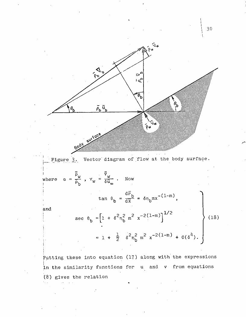
\ 30

I>

eb

Bb b b

Figure 3. Vector diagram of flow at the body surface.

p vw wwhere a = , Now

b 6

dr -(l-m)tan 6 - = 6bmx

b dx b

and

2sec 2 2 -2(1-m) 1/2se = + 6 n m x (18)

1 2 2 2 -2(1-m) 4= 1 + J nb m x + O(6 ).

Putting these into equation (17) along with the expressions

in the similarity functions for u and v from equations

(8) gives the relation

31

[o(b) - b] m-(1-m) - tv w

2

+ 6b [2(nb) - lbvol m - Cvw Z- m (19)

-(1-m) 4+ (nb ) m-( l - m ) + 0(6 ) = 0

If the flow through the surface has the particular form

vw = wm - ( -m ) , where w is a constant, the boundary

conditions at the body surface are (from equation (19))

o(b ) - b - 0

2

Snb2 w = 0 , (20)

Ol(nb) = 0

While the-development of these boundary condition shows that

mass flow through the surface can be accommodated without

difficulty, the rest of this dissertation will be restricted

to the no mass flow conditions, 4w = 0. The resulting

boundary 'conditions are

qo(n b ) - b = 0,

2 - nbvo(rb) 0= , (21)

l( b) 0.

Initial magnitude checks. These boundary conditions

can be used with the flow equations to provide some initial

checks of the order of magnitude of the similarity functions.

As stated in Section II-B, these functions have been

assumed to be of order unity. From the boundary conditions

at the shock (equations (15)), this assumption appears

justified there, for- y not too close to one and if a2 is

not too large, except that ' 2 (ns) = 0. Having a function

become much less than one does not invalidate the procedure

used in getting the equations so long as the function does

not appear as the denominator of terms that one dropped as

being negligibly small, i.e. of order 6 . Neither i2 nor

any other order- 62 function is in the denominator of any

term that is dropped.

Solutions to the zeroth-order equations given by

Kubota (9) indicate that F and o remain of order one0 0

from the shock to the body but that 0 goes to zero at

the body surface when m < 1. This result could affect the

validity of the solutions in the region where is small

33

since does appear in the denominator of a number of

terms of equations (10) - (13). One of these is the zeroth-

order lateral momentum equation (11). Applying the boundary

condition o(nb) - b = 0, this equation becomes

b bF'( b )

from which F'(nb) = 0. The zeroth-order longitudinal momen-

tum equation (11) multiplied through by 'o is

(n - ) + + 2(-m)(v + Fo ) = 0.0 00 0 m 00 0

Using (b - b = 0 and Fo(nb) = 0, this becomes

v~ o(nb ) + Fo(n o) = 0 . (22)

Since 'o(nb) = 0 and Fo ( b ) 0, this requires vo m

as n ob . Thus there is a (non-physical).singularity* in the

similarity solutions at the surface of the body n = nb.

One possible way to avoid the singularity at the body

surface is to reformulate the problem. The fact that voP o

which remains finite as n + nb , is the zeroth-order

similarity form of the longitudinal momentum suggests that

*Kubota (9) and Mirels (10,16) do not encounter this problembecause they omit the variable vo entirely. It only occurs

i.in the longitudinal momentum equation, which they do notuse, prefering a Bernoulli equation for the velocity.

3 4

using momentum components, instead bf velocity components, as

fundamental variables might remove the singularity. This

approach is pursued in the next section.

D. Momentum Variable Formulation

As was noted in the previous section, the zeroth-order

longitudinal velocity similarity function v is singular

at the body surface. However, the product o vo remains

finite, which suggests that a reformulation of the problem

in terms of new variables might remove the singularity and

allow the numerical integration to.proceed all the way to

the body surface. The variables chosen for the reformulation

are the longitudinal momentum pu (which is expected to

behave like vo and so remain finite at the body surface),

the lateral momentum pv, the pressure p, and the density

p. In terms of these variables, the inviscid flow equations

(1) become:

Continuity: 8pu +a pv V - (23a)ax ar r

Longitudinal momentum:

8pu - v -pu ) +-2 p (23b)pu Px p u -- + p(p - _ pu p - !(.23b)

? .ar

* 35

Lateral momentum:

-apv p pv -2 BP (23c)pu(p - x + pv v)+ p = 0 (23c

Energy: (pu y + pv -) (P-Y) = 0 (23d)

Normalization. These equations are normalized using

the expressions:

x r P P"x-= - , r = - , p = 2- r pE 2 2

(24)

p , (pu) Pu (pv) =- --O Pu - 6p o u

'(Note that these expressions are the same as equations (2)

with the exception that (pu) here is the same as the previous

p(1+6 u).) The normalized forms of the equations (23) are

then:

D(pu) (p) ) (25a)Continuity: (u + (p) + (p) 0(25a)ax .r r

Longitudinal momentum: (pu) [p (pu) (pu)

(25b)

+ (pv) pu) - (pu) r+ 6 P 2 = P-(ru aix

36

Lateral momentum: (pu) [p PV) - (25c)3x x ( 25c)

(py) p 2 3par ar arS-(pv) (P--. 0 (25d)

Energy: pu) + (pv) r P = (25d)

Similarity variables. Just as in the first section of

this chapter, the similarity forms of the momentum variables

are chosen using the relations for flow through an oblique

shock wave as guides. Combining the density and velocity

relations used previously (equations (4)) gives the follow-

Ing relations' for the normalized variables just behind an

oblique shock:

S2. 2 2 2(pu) (y+l) MC sin a 2(M sin 0 -

u EPUs 2 s2 _ 2p~- (y-l) M sin - 2 (y+) M

(Y+l + 1 )+ 6 2 R' 2 (+l + 1)2 '( 2 6a)

1 1 )(1 + 2 R 22 M2 M2 2R 2 + 6

y+l 6 2 2 R2 + 2(y+l) (R')- 2 + 0(64)y-1 Ry-1 ( 2

37

(pu) s 2 (y+l) M2 sin 6 (M sin s - 1)

s22 2 S6 (y-1)M 2 sin + 2 (y+l)M2 tan 8

R 2 (1 + 6 2 R ' 2 ) R'(26b)C O 2J(26b)

SR'- 2 M 2 (1 + 62R '2 ) (1 + 62R 2)

2 2 3 2 (y+l) R 1 + 0(64)

S R' -6 R' - + 0( )Y (y-l) 2

The similarity forms of the momentum variables are. taken to

be:

S+ 62 2 (r)(R)pu = u (r) + 62 u2r)R' + E u(r)(R')-.

and (27)

2 2-1pv = i (r) R' + 62 2 (r)R'3 + 5(r)(R')

Using the same perturbed, power-law shock wave shape as

before (equation (7)), these become (for e<62)

i-npu = o(n), + 62u2(0) m 2 ( + I () 2(-m) + 0(64)

m

and

pv = + o(n) mr +) m62 -3(lm) + p ) (

+ 0(6 )

38

The similarity forms of .p and p are unchanged from the

previous formulation ('equations (8)). Putting the similarity

forms of these variables into the flow equations (25),and

using the chain rule for partial derivatives (equations (9))

as before, produces:

Continuity: (p - nu + - ) m-i

: (29a)2 1-m 3 2m-3+62[p - nu - 2( ) U2 + 2 m

2 m 2

+ E[Il - u1 + 2(1- m ) 1 + 1 1 (1-2m)+ 0(6) = 0

Longitudinal momentum: (nu - 1o)(u 4' - 41o u) m

+ 62{(niu - )(u , - ou') +0 o o 2 0 2

1-m 2[2(- ) u - (nuo - o )u ] 2 + ( oU - Uo )p

+ [(au - o )4' + n(u 4o - , u') - 2(1-m), u]o o 0 0 0 m oo 2

2 3 2M-3 (29b)- 2 [nF ° + 2(-m F]} m32m 3

o o

+ - i )- u ) - [2(1-m) 2o 0 o 0 1 m o

+ (nu - P )Uo] + (u- uo )

+ [(nu - V )' + n(u o' - 4 u')

l-m 1 (1-2m) 64 .+2( ) U] ul} - + 0(6 ) = 0.

39

Lateral momentum:

2 -m m 2m-2[(nu ° - 0 )(v'0 - PFI ) + o - (--) o vu 0

] m

2 0 o o2 o 2 oF2

+ [2ioF' - (Tu ° - po)pv + ( >)po uo]20 0 0 0 m oo2

1o(no - o)' + ( )' - v ') 4 ( r)0 0 o0 0 0 m 00 2

,+ [P~(p '1-m) ' ) )4 3m-4(2+ 0 00 m o0 0 2 2

+ E{(nuo - v )(p o - p i) + F0 0 0 o ol ol

+[2 - (fu )% ) - 3(-)oup 1

+ [( - v ) P' + ('P ' - v ' ) + (-m) u~O 0S[o o ) oo m + 0(64

+ [n(v p - it) ( m) p u -m 0(64) - 00 0 '0 0 m 0~ 1

40

Energy: [(qu - p )(YF 4' - F) - 2 (1-m)F q 32nm-3

0 0 00 00 m 000

+ 62{(qu ° - P )(YF 0 ' - o F') + [y(Iu o - o ) '

L 4( ) oUo] F2 - (yFooo - 'F 2

[(nuo -1) F' - 2(m )(Y-1)FoUo] 2

+ [n(yFo, - ,oF') - 2(i-m) Foo] °2} m5S~m-5

,(29d)

+ E{(nqu - po)(Fo{ - 4oF{) + y(nuo - po)4F0 0 o 0 0 1

[(u -- -)2' -+2(l- m ) (y+)F u

S[n(F 4 - o F') - 2(1-m) Fo ol00 00 m 00 1

-(YF oI O- ) 1} m-1 + 0(6 ) = 0

Zeroth-order equations. Using the same reasoning as was

employed in Section II-B, the coefficients of the zeroth-

order term, the order-62 term, and the order-c term of each

of these four equations must be equal to zero. The

zeroth-order system of equations which results from

recognizing this fact is:

0 0Continuity: Jo - Uo 'o = 0

Longitudinal momentum: (nu - I )(o ' - o ') = 0

Lateral momentum: (30)

S- ) + 2 F' ( ) u = 00o o 00 o o m ooo

Energy: (nuo - )(yFo~' - o FT ) - 2(1-m)F i = 00 0 oo 00 m 00o0o

The longitudinal momentum equation can be integrated

immediately. For (nuo - o) 0 (i.e. away from the body

surface; see next section), it becomes Uo P - 'oup = 0,

which has the solution, uo = C0o . Comparing equations (26)

and (28), the boundary condition on uo at the shock wave

is uo(fs) = +l Thus, with o(ns) given by equation (16),

the constant c is

uo(n) y+l1c- o s y-1 = 1

o s ( +l)and y-1 (31)

o 0

(This result could have been anticipated by making a

comparison of the similarity variables for the two

formulations as given by equations (8) and (28).)

Using the results just obtained, the three remaining

zeroth-order equations may be written:

11 2

Conti nuity: - - = 00. 0 fl.o

Lateral momentum:

') + [F' - ( ) (32)

Energy: (ro - o )(yF 0' - ,F'o) - 2 (m 2oF = 0

2Order-6 equations. Also using the result uo = o

the order-6 2 system of equations may be written:

Continuity: 12 - u - 2( m) U 2 + 2 = o33a)

'Longitudinal momentum:

(o 0 - I)o JI -p ) + [2(1-m)i - o -

(33b)

lm),2 2 2 2( 1 ] = 0+ [(qo o ) ' - 2(1 ']u [nF + 2(- m)F] =

0 0 M 0 2 o

Lateral momentum: (nqo- po)(Po2- opI) + 2F2

+ [io(2F + ( - -0 m 0 2

(33c)

+ [(ni - o) + (lP. - o' ) - 3( )]

-_ oP ) - (L -) i oO)

[ ( o o m o 2

+ I 11 l o 1-m) ou 00 0 0 0 m 0 0

43

Energy: (o - o)(yFo2 - o2 Fo - 2

+ [y(rno ) p - 4 (1-m) 2 ]Fo o m 0 2!(33d)

- [(n - o) F' - 2(1-m)(y-l)F o]0 0 0 m 00 2

+ [(yF - F) - 2(1-m)F = 000 0o m 00 2

The order-c equations governing the shock wave strength

.perturbation are very similar and could be written in the

:same manner, but since they are not needed here they will

not be derived.

Since the physical momentum component variables are

simply the products of the density with the velocity com-

ponents in the usual formulation, the similarity functions

of the two formulations are simply related. Noting that

the normalized momentum variable (pu) is equivalent to

;p(l + 62u) in the previous formulation, the relations between

'the similarity functions are:

Uo b Po' oo' u2 =2 - o, and 12 =o2 + o2

(34)

Boundary conditions. To determine the boundary condi-

,tions for the momentum variables, equations (28) must be

compared to the expanded form of equations (26). Putting

the shock wave shape (equation (7)) into equation (26) and

expanding gives

_ y+l 2 2 2 -2(1-m) 2(y+l) 1 2(1-m) 0(64)(pu) Y 6 m2 + 2 + 0(6)

s y-1 y-1 (y-1)2 m

(35)

2 -(1-m) 2 2 3m-2 - 3 -3(1-m)(PV)s -1 m( + 6 [a2(3 ) ]m (

2 2[(-m + l] 1 (l-m) + (64+ s [()a + - + o( )

y-1 M 1 Y-1 m

iThe term-by-term comparison of these equations with equations

'(28) gives

=2 2 2 3m-2os ) y-1' u2 s) -l' 2(s Y- m )a2 - 1]

(36)

The boundary conditions at the shock on P0 , *2 , Fo, and F2

are the same as given by equation (15). The boundary condi-

tions at the body are determined by the mass flow through

:the surface, as in the previous formulation, Section II-C,

'In this case, when equation (16) is normalized in terms of

the momentum variables it becomes:

(pv)b = (pv)w sec b + (pu)b tan b (37)

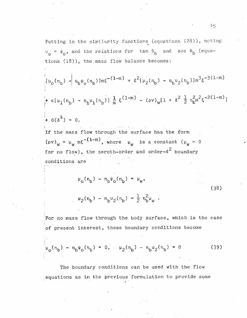
Putting in the similarity functions (equations (28)), noting

Uo = o and the relations for tan 0b and sec 0b (equa-

tions (18)), the mass flow balance becomes:

l(o(ib) -nT o(nb)m-(l m ) + 62 3 - 3 (1-m )

1 (1-m) 2 1 2 2 -2(1-m)b+ l(nb ) - bul(b)] m w 2 bm (

+ 0(6 ) = 0.

If the mass flow through the surface has the form

-(1-m)(pv) w= m( , where Pw is a constant (pw = 0

for no flow), the zeroth-order and order-62 boundary

conditions are

Po(n b ) - b bo(b ) = w

(38)

-0 1 212( b) bu2 b 2 b w

For no mass flow through the body surface, which is the case

of present interest, these boundary conditions become

o(nb) - o(b) 0, 2(b) - nbu2(b) = 0 (39)

The boundary conditions can be used with the flow

equations as in the previous formulation to provide some

46

initial checks of the order of magnitude of the similarity

variables. At the shock wave, the boundary conditions

(equations (35)) indicate the variables are of order unity

there. At the body, the zero-order boundary condition

(equation (39)) produces the same results from the zero-

order energy equation (32) as before; i.e. 0o(nb ) = 0.

Thus the boundary condition at the body (equation (39))

becomes P( o) = bo(nb) = 0; but vo( b/ (ib) = n b in

agreement with equations (34) and (21).

The development above shows that it should be possible

to get order-6 2 similarity solutions using the momentum

variable formulation, and that this formulation avoids the

,singularity in the .zeroth-order longitudinal velocity at the

body surface. Whether the formulation is successful in

'avoiding singularities in the order-62 variables must be

determined from the numerical solutions to be obtained.

E. Correlation of Solutions

Hornung (26) suggested a method to nondimensionalize

experimental data so that shock wave shapes and pressure

distributions for a given body power-law exponent would each

form a single correlation curve. The basis of his correla-

tion is to nondimensionalize the shock coordinates by a

length scale D defined such that the body shape is given

by

rb (m

1m 1 m

For rb bx , D = (6nb )

When this' correlation is applied to the order-6 2 similarity

!solution shock-wave shape, given by

S= 1 + a2m

.the shock shape becomes= a i )m ) 2 ( )- 2 (1 - m)

D_ D 2 x,-R 'l t~ 1 + a2 )) ]

Since this equation does not contain the slenderness parameter

6, it gives a single curve for any given value of the body

power-law exponent m; i.e., the order-S 2 similarity

solution produces a single correlation curve independent

of the value of the slenderness parameter 6.

Hornung suggested that pressure data would correlate in

'much the same way if it were plotted as T/p~ ~ vs X/D,

where D is the same non-dimensionalizing scale length

as used for the shocks. In fact, the order-6 2 solutions

:show that not only the pressure, but also the other flow

:variables correlate when x/5 is the longitudinal distance.

'The pressure, density and velocity components from

equations (8) can be written

48

S-2(1-) -- 4(1-m)S26p = 262 Fon2( ) + 62 2m (-)

-2 x -2(1-m) 4 4 4 -4(1-m)-= 2 Fom262 (b) (- ) + F m 6(6b )

2 - -2(1-m) 4 - -4(1-m)S 2F ( ) (x) + 2F (m ) x)

0 b D 2 b

-2(1-m)P 2 2==o+6 )

2 - -2(1-m)= + ( ) G=)

[-2(1-) 2-4(1-m) 1

2 - -2(1-m) 4 - -4(1-m)= 1 + v() () + v2 (a )

0 ob D 2r Dand

O (1 -m) -3(1-m)-6v = 6 om(-) + 62 2m ( )

S-- (-(1-m) +3 -3(1- m )

= () +20 Tb D 2 b

,Since none of these contains 6 explicitly, each one forms

a single curve for a given value of the body power-law

:exponent m, independent of the body slenderness. Thus it

should be possible to correlate experimental velocity

component and density distributions, as well as the pressure

distributions, by plotting them against the normalized

coordinate x/D.

The regularity of the correlation form for expressing

the physical variables in terms of the similarity functions

suggests a possible refinement of the similarity formulation.

By using the local zeroth-order shock wave slope, expressed

as

-' - -(l-m)R m (X=b

1as the small parameter instead of the average shock wave

slope 6 = Ro(7)/T (Figure 1, p. 13), it should be possible

to improve the formulation. In particular, this change

!would facilitate the estimation of-error in the nose region,

,where the local shock slope increases rapidly. While it has

not been possible to include it in the present study, such

a reformulation would provide a good starting point for

further work on similarity solutions in hypersonic flow.

CHAPTER III SOLUTION OF EQUATIONS

A. General Scheme of Solution

Either the velocity-variable or the momentum-variable

similarity form of the flow equation ((11) and (13) or (32)

and (33)) with the boundary conditions at the shock wave

(equations (15) or (35)) and at the body surface (equations

(21) or (39)) is sufficient to completely determine a

solution for the flow field. However, since there is no

general analytic form for the solution in either formulation,

it must be found numerically for each case (i.e. for each

value of the power-law exponent m with a set equal to

either zero or one).- The general scheme for obtaining the

numerical solution is to begin at the shock r = rs, where the

boundary conditions are known, and to integrate the similarity

functions numerically toward the body, which is known to be

reached when the zeroth-order boundary condition is

satisfied; i.e., n = nb when

So(n)o(n) = n or -o = n •

The derivatives of the similarity functions, used for this

integration, are found by solving the flow equations for

them algebraically. Thus, from the zeroth-order equations

(11), the derivatives are

50

F'(r) = om - 2(m ( Lo _ 2 mo o a- im

y-(n-00 )

SYF (n= o +2( F

(40)F' FV'(n) 1- -1 + 2( )(v + )o n- o 1 m

1 o 1-m(n ) - ( ) oo n-o m

The derivatives of the order-6 2 functions, from equations

(13), are

F'La l-m ,) _ 0

(n) =1 n-o (3m oo 0

2 2 F' F

0 ; Pm 0 (4la)2 2o l-m 2 -

+ (n- o ) ( + 2( + yn yo o o m F o (0 a

+(--4) -m o + 2(y+l)(-m

0 o F

=?- o - )r + [3( -m) 2

(41b)

+ + (~> o]vo + F

52

9' -d_ + -m - 2( )2 + o9 22 0 o om 2 0 2

(41c)

+ (~ + 2-)v - I(v p + -m 'S l 2 m 00 00 o 0

2 n-1 o 2 F2 m 2So (41 d)

F F' Fo -m o 2 1-m 2 1+ l( + n -F 4( )

0 o o

Similarly, the derivatives of the similarity functions for

the momentum variableformulation are, from equations (32)

and (33):

O Fo 2( o o

1 o 2(1-m)

'F' + 2( ) im /(no yI F o m O

ot' + [F' (-m) O)0 (0 ) ol

and

53

0I 0

+ 1- m+ yo( 1-m o+ 2(0m0 2 ( +U2 m 0

0 o

S= 1-PF + F-)o yl -(') o F

(n3 I°)0o (43b)

+ (n ) n )2 + (nu + (43a)

L O 0 OM) -

So Po

= (2F + ( o)(go - o)) 2]- yn F' -2 2()1

n '+ - )o F2

0 o+o 2 (43b)

+ '- yF o - )+ (2 1 2 (

(n - -) ,

2; = 7; 2 2 ( m 2

514

Two major difficulties must be overcome in order to

apply the scheme of integrating either equations (40) and

(41) or equations (42) and (43) from the shock to the body.

One difficulty is the singularity at the body surface

apparent from the fact that the denominators of some of the

terms of these equations approach zero as the independent

variable n approaches the surface value b. It was over-

come by using an approximate analytic solution, developed by

Mirels (10) and described in Section B of the Appendix to

calculate the value of ob and the zeroth-order similarity

functions in the region very near the body surface. For

reasons explained in Appendix Section C, the second-order

variables are calculated at the body by extrapolation of

the order-6 2 similarity functions. The extrapolation techni-

ques used are described in the next section. The second of

the two major difficulties is associated with the fact that

the problem is a two-point boundary value problem. This

difficulty is manifest in the need to choose initially the

correct value of the shock wave displacement parameter a2

(equation (7)) in order to satisfy the order-6 2 boundary

condition at the body surface when n = rb at the end of

the integration. The steps taken to deal with this diffi-

culty are described in Section C below.

0 - n + 0 as n + nb from equation (21).

55

B. Extrapolation of Order-62 Functions

Two simple extrapolation techniques were used to carry

the order-6 2 similarity functions the short distance from

the last computed point to the body surface. For the

velocity-variable formulation the extrapolation used for

each of the functions F2' 2' 2 and v2 was a cubic

function of n passing through three computed points of the

function and having zero curvature at the body surface.

The points used to define the curve were the last computed

point and two previously computed points. The number of

steps between the points was the next integer larger than

the distance between the last point and the body divided by

the last step size. - -

For the momentum-variable formulation, the functions

F2 and u2 were extrapolated linearly to the body surface

using the last computed point and slopes. The order-62

stream function e2 and its derivative were also calculated

at the last point, using the momentum-variable form of

equation (A9), and 62 was also extrapolated linearly. The

values obtained were then used in equations (34) and (A8)

to calculate *2(n b ) and 2(n b ) '

C. Methods for Determining the Constant a2

Since the constant a2 is initially undetermined, the

value of the order-6 2 shock wave similarity ordinate

'The results are insensitive to the technique (Section IV-B).

56

s = 1 + a2m 2( ) is unknown and cannot be used to

begin the integration toward the body surface. Also, this

shock ordinate varies with the longitudinal distance E, so

that its use would require a separate solution for every E

value. The use of the zeroth-order shock ordinate n = 1

as the starting point for the integration avoids these two

problems in determining the initial value of ns but requires

that the boundary conditions be transferred to r = 1 from

n = ns, the order-6 2 shock position, where they are known.

This transfer is made by using the Taylor series expansions

of the similarity forms of the flow variables about the

point n = ns in the same way as Kubota (9) and Mirels (10)

did for the order-c.perturbation. The Taylor' series expan-

sion of-a general function g(n) about ns is

g(r) = g(n s ) s ( - ns) + ns( 2s2...

Applying this expansion to equations (8)(with terms of order

c neglected) and evaluating at n = 1 give

p(,l) = Fo(ns)m 2(l- m) 6 2 [F (ns) - a F'(ns)]m4 -- 4(1 -m )

Ss(44a)

+ 0(6 )

p(,l) = () 0 + 62 [ 2 (ns ) - a 2 Vp(ns)]m 2 -2 ( 1-m ) + 0(64) (44b)

57

u(,1) = v (ns)m2 2(1-m) + 2[v2 ) - a2' (n )]m ' - 4(1-m) (44c)

+ 0(6 )

v(E,4)= ,(nsr)m-(1-m) + 62 2(-s ) a23 o( s)]mB-3(1-m) (44d)

+ 0(64)

Similarly applying the Taylor series expansion to equations

(28) gives

(pu)(,l)) = (n 2[+ 2 (n - a2u(n s)]m2 - 2 (1 -m ) +0(64)

(45)

(pv)(E,l) = 1 (ns)m (l-m) + 62[1p2 (n) -' a 2UO ]m33 E- )-

+ 0(6 )

Evaluating equations (8) at n = 1 directly and comparing

the results to equations (44) and (45) yields boundary

condition transfer relations of the form:

Fo(1) = Fo(ns), F2(1) = F2( s ) - a2F(s),

So(1) = 9 0(ns), ' 2(1) = 2(ns ) - a2o(ns),

etc.

58

Putting equations (40) in for the derivatives and applying

the boundary conditions at ns (equations (16)) gives the

transferred boundary conditions at n 1:

2 (+1) (1) 2 -2Fo(0 ) = (1) = y+l' o (1) = y-1 y+l

S2 2 3m-2 (1-m)(2Y-1y) + yF2(1) - ( - ( ) + a - 1

(1)2 3(1-m Y+ - a]a (46)2 y-1 m Y-1 2

_2 3m -2 -m 1 fa vV 2[(31-=2) - (_m) + -a -

2(1) y+1 m 1 +1 2

2 3m-2-m 1 + ayla 12 7m m y+1 .2 -

Similarly for the momentum variables (equations (42) and(36):

(1) = 1 2 (1) =

2 (1) - 1 [3(1) - a 2 + 1 (47)

P2(I) = y---" rn2 - 3(i!) _(ii + 2ala2 .11

59

Iteration method. These transferred boundary conditions

provide a definite starting position for the integration

toward the body, but the constant a2 must still be deter-

mined. There are two methods for determining a2 . The more

obvious one is to guess the value of a2 , integrate toward

the body (using the method given in the previous section to

reach the surface), test the order-62 boundary condition

at the surface, and repeat using improved guesses until the

surface boundary condition is satisfied closely enough.

The improved gusses for this iteration method were made

using the method of chords, a finite difference approximation

to the well known Newton-Raphson method. (Note that the amount

by which the boundary condition is not satisfied corresponds

to the mass flow through the surface according to equations

(20) or (38)..)

Decomposition method. The other method for determining

a2 takes advantage of the linearity of the equations in

the order-6 2 functions, which allows superposition of

solutions. It was used by Sakurai (4), Kubota (_9), and

Mirels (10) in obtaining their results and is applied in a

similar manner here. Each of the order-6 2 similarity

functions is decomposed into a linear combination in the

parameter a2; e.g.

60

F 2 (n) = F 2 a(n)a 2 + F2'(),

(48)

2(n) = 2 a(n)a 2 + 2c(n), etc.

Splitting each of the equations obtained in this way into

two separate equations, by setting the term containing a 2

and the other term each equal to zero, produces a system of

equations in the subscript-a functions and a system in the

subscript-c functions. The system in the subscript-c

functions is identical to the original system of equations

(13) or (33). The system in the subscript-a functions is

the same except that the inhomogeneous terms (i.-e. the terms

that do not contain an order-62 function or its derivative)

do not appear. These two systems of equations have two

different sets of boundary conditions. In order to obtain

them, the boundary conditions at n = 1 (equations (46) or

(47)) are decomposed by comparisons with equation (48),

giving

F2a (1) = (3m-2 1-m) (y-1 Y], F2 (1) 2 (49a)2a +l m m -1 y+1 2c y+l

(1) 2 [ -m y+') - o], 12c1) = (49b)2a Y-1 m y-1 2c

4 3m-2 (1-m (1 2 (49c)V2a(1) = [( ) (l)( ) + ] v2 () y+l

61

[() 2 3m2) +2 y ], (1) 2 (49d)y+ m m y+1 2c y+l

or,

(1) - 13(1-m)(Y+) a , = (1) 22a y-1 m --1 2c y-1

(50)

a( 1 ) 2 [(3m )- 3 ( 1m)(Y+) + 20], 2c(l) - 22a Y-1 m m y-1 2-1

These decomposed variables are then substituted into the

order-62 flow equations, so that the continuity equation (13),

for example, becomes:

1o + + - 12 0 2+ 2a 0 0 2a o 2a

S+ 2(1-m

0 o m 2c, o

+ , + o + 2(- )] 2c1-

- [nvo + 2 (1-m)v ]4o = 0o m oo

Beginning at n = 1 with these boundary conditions, the

decomposed system of equations (in either the velocity

variables or the momentum variables) is integrated toward

62

the body. Near the surface the method given in Section III-B

is used to obtain values for the decomposed functions at the

surface. The boundary condition at the surface, expressed

in terms of these surface values of the decomposed functions,

is (from equation (21))

2a(nb)a2 + 2c(nb) - nbvo(nb) = 0

or (from equation (39))

1[2a(nb ) - n bu 2a(nb)]a2 + [b2c(nb) - nbU2c(nb)] = 0

Thus, in the velocity-variable formulation, the value of a2

is found from the relation

a =( ) (51)22a b

In the momentum formulation, a2 is

nb2c(n b ) - u2c(l b)a 2 = - (.b) - (rb) (52)

nbu2a b P2a b

The value of a2 is now used to recombine the decomposed

similarity functions using relations such as equations (48).

Once these functions have been computed for any value

of the body power-law exponent m (with a = 0 or 1), they

63

can be used to calculate the complete flow field about

any such body as long as it is slender enough that 64 << 1

and the Mach number is large enough that E << 1.M22 "

D. Description of the Numerical Method

The equations derived in the previous sections of this

dissertation have been programmed for numerical solution on

the CDC 6600 digital computer at the NASA Langley Research

Center. Three separate programs were written, correspond-

ing to three of the different methods of obtaining solutions

which have been discussed. Two of these programs integrate

the velocity-function equations (40) and (41); one uses the

iterative and the other the decomposition method for obtain-

ing the value of a2. The third program integrates the

momentum function equations (42) and (43) and determines a2

by the iterative method. All three of these computer pro-

grams use a standard integration subroutine employing the

fourth-order Runga-Kutta formula supplemented by a Richard-

son's extrapolation. This subroutine halves br doubles the

integration step size automatically in order to meet a

specified local truncation error.

For the present computations the initial step size (in

a) was 2- 8 (.00390625), and the maximum allowable step size

was 2- 7 (.0078125). Generally the step size decreased to

less than 2-15 near the body. At each step estimates of

nb and Fo (Ib) were computed by t'he method given in

Appendix Section B (equations (A18)). When both estimates

agreed to within 1.0x1 0 on successive steps, the estimates

were accented as the actual values of nb and Fo (nb ) and

the values of the other functions at the body were computed

from the approximate analytic solution given in Appendix

Section B or the extrapolations given in Section III-B. The

iterative programs used a "method of chords" algorithm to

compute improved estimates of the values of a2 . (This is

a finite difference approximation to the well-known-Newton-

Raphson method). The iteration was considered to have con-

verged when the order-6 2 boundary condition at the surface

(equation (21) or (39)) was satisfied to within 0.5 x 10- 10.

CHAPTER IV. DISCUSSION OF RESULTS

A. Zero - Order Functions

The methods given in the last chapter have been used to

compute the zeroth-order and order-62 similarity functions

for a number of cases, which will be presented and discussed

in this chapter. Unless otherwise noted, these cases are all

for y = 1.4, representing air as an ideal gas. The Figures

presenting the functions were plotted by Calcomp plotting

machines directly from the computed results. The.slight

waviness which may be noticeable at some points in the

Figures is a result of this computer-aided plotting process;

however, the curves at all points on the plots are accurate

to within 0.1 percent of the full scale values.

The zeroth-order similarity functions Fo ' , and

V0 are shown for several values of the power-law exponent

m in Figure 4 for two-dimensional flow (a = 0) and Figure 5

for axially symmetric flow (a = 1). These functions agree

with the same functions calculated by Kubota (9), Mirels

(10,16), and Townsend (23).

The pressure function Fo and the lateral-velocity

function o are seen to be smooth and well-behaved from

the zero-order shock location (n = 1) to the body surface.

Note that the body surface values of @ lie on the line

o = n in accordance with the zeroth-order boundary condition

65

66

1.0

I.3

m= 1.00

.8 -/ 0.95

/ /90

.7 Body surface values _ 0.

.64

0.70

.3-

.2 -

.1

n I I I I.5 .6 .7 .8 .3 1.0

77

(a) Pressure function, Fo(rI).

Figure 4. Zeroth-order Similarity Functions for Two-Dimensional Flow (a = 0).

67

10

9-

8

7-

m= 1.00

0

o 5-

3-

2

1

.5 .7 .8 .9 1.0

(b) Density function, o(n).

Figure 4," Continued.

68

0.95

Lo -1 .0- 0.70

-1.2 -

-1.6 -

-1.8 -

-2.0 I I I.5 .6 .7 .8 .9 1.0

(c) Longitudinal velocity function, vo().


1.0

.9

m =1.000.95

0.90

0.85Body surfoce values /

.7 0.80

.6- 0.75

'o .5 --

00

.3

.2

.5 .6 .7 .8 .9 1 .0

(d) Lateral velocity function, 4O().


1.0

m= 1.000.95 1 0

.80

*7(a Body surface values Oto

.6

FO .5

.3-

.2

.1

.75 .80 .85 .30 ..95 1.00

71

(a) Pressure function, Fo(n).

Figure 5-. Zeroth-order Similarity Functions for Axisym-metric Flow (a = 1).

71

10

9

8

7

m= 1.00

609O

3

2

1

.75 .80 .85 .90 .95 1.00

(b) Density function, to(n),


72

0

-.2

-.6

-.8

m = 1.000.95

vo -1.0 -

-1.2 -

0

-1.6 -

-1.8 - 0

-2.0 I I.75 .80 .85 .90 .95 1.00

77

(c) Longitudinal velocity function., vo(n).

Figure 5. Continued,

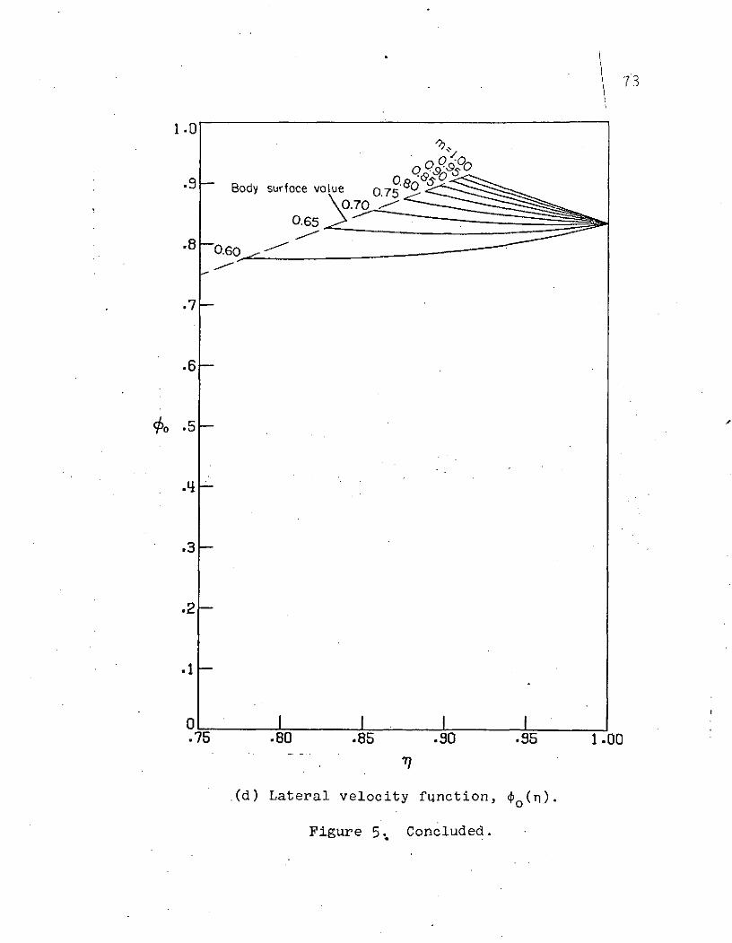
73

1.0

•9 Body surface volue 0.750.70

.6

€o .5

.3

.2

.1

o I I . I I.75 .80 .85 .90 .5 1.00oo

17

.(d) Lateral velocity function, ~0(n).


74

(equation (21)). As expected from the discussion in Section

II-C, the density function o and the longitudinal velocity

function v exhibit different types of singular behavior at

the body surface for m i: io goes to zero, and vo goes

toward minus infinity. From the Figure it appears that the

effects of these singularities are confined to a thin layer

near the body surface, at least for values of m near 1.

The zeroth-order lateral momentum function P is

shown in Figure 6 for both the planar and axisymmetric cases.

As indicated in Section II-D, the longitudinal momentum.func-

tion uo is the same as the density function o0 , and the

pressure and density functions, F and po are the same as0 0

in the velocity-variable formulation. In the separate 'cal-

culations made for the momentum-variable formulations, these

functions came out essentially identical to the previous

calculations, Figures 4 and 5. The function 110 is seen

in Figure 6 to behave like po, in agreement with the com-

parison of methods in equations (34). Thus the reformulation

in terms of momentum variables was successful' in avoiding

the unlimited growth of vo near the body surface.

B. Shock Displacement Constant

The variation of the calculated order-6 2 shock wave

displacement constant a2 with the power-law exponent m

is shown in Figure 7(a) for both two-dimensional and

75

10

9-

8-

07

6-

.o 5 .6 . .8 .00 .

3-

(a) Two-dimensional flow (a 0 0).

Figure 6: Zeroth-Order Lateral Momentum Function, W.

2 _ 4

1-

Figure 6. Zeroth-Order Lateral Momentum Function, gon)

76

10

9-

8-

7-

6-

4-

2-

1-

o I

.75 .80 .85 .90 .95 1.00

(b) Axisymmetric flow (a = 1).


77

axisymmetric bodies. The calculations made using the itera-

tive method for obtaining a2 gave essentially the same

values as were obtained by the decomposition method (equations

(48) - (52)). As can be seen in the Figure, the momentum-

variable formulation results for a2 differ only slightly

from the results of the velocity-variable formulation.

However, all of the results are characterized by a singular

discontinuity in a2 which has no physical counterpart in

the actual flow about power-law bodies. This singularity,

which occurs near m = .817 for a = 0 and near m = .653

for a = 1, represents a rapid decrease in the distance

from the shock to the body as the power-law decrease,

followed by a jump to a large distance at the discontinuity.

Since this behavior is physically unrealistic, it must be an

artifact of the mathematical processes (analytical and

numerical) used to obtain the solutions.

Figure 7(b) shows.that the singularity is associated

with a zero in the denominator of equation (51). (This is

the equation used in the decomposition method to determine

the value of a2 satisfying the order-62 boundary condition

at the surface.) Since there is a nearby zero in the

numerators of this equation, it is probable that the

singularity in the quotient a2 occurs because the zeros

in the numerator and denominator, which should coincide, are

displaced relative to one another. (Coincidence of the

1.0a.OO

elocity.8 - formulation

Velocity formulotion

- Velocity

-.2- (Momentu Comulte -elocity lotion

.6

Figure 7. Variation of Shock Displacement Constant a2 with Body Power-Law

.60 .65 .70 .75 .80 .85 .90 .95

1.0

.8 02

.2 -

0

-.4 I I I I.60 .65 .70 .. 75 .80 .85 .90 .95 1.00

Body power-law exponent, m

(b) Numerator and denominator of expression for -a 2 (equation (51)).


80

zeros would make a2 mathematically indeterminate at that

point but would allow a continuous variation of a2 with m,

from which the value at the indeterminate point could be

'inferred.) The most likely causes of such a zero displace-

ment are accumulated truncation errors from the numerical

'integration and errors in the extrapolation from the last

!integration point to the body surface. Any error occurring

,in these processes is aggravated by the fact that the

Inumerator of equation (51) is the small difference of two

nearly equal extrapolated numbers. For example, with a = 0

and m = .83, nb = .73327 and the extrapolated values

v (n b ) = -9.9910 and -2c(b) = -7.3153 give the numerator

--0108 with--a relative error about 1000 times that of the

individual functions; that is, an 0.1% error in vo(nb)

,and #2c (b) would become a 100% error in the numerator of

equation (51).

To test this line of reasoning, additional calculations

were made reducing the step size, reducing the range of the

extrapolation, and finally, extrapolating the whole numerator

of equations (51) rather than just the separate parts. The

!results of these calculations indicate that the value of a 2

is sensitive to these changes for power-law exponents less

than that at the singularity; but, the position of the

singularity and the values of a22 for m greater than that

at the singularity were virtually unaffected. Thus, removing

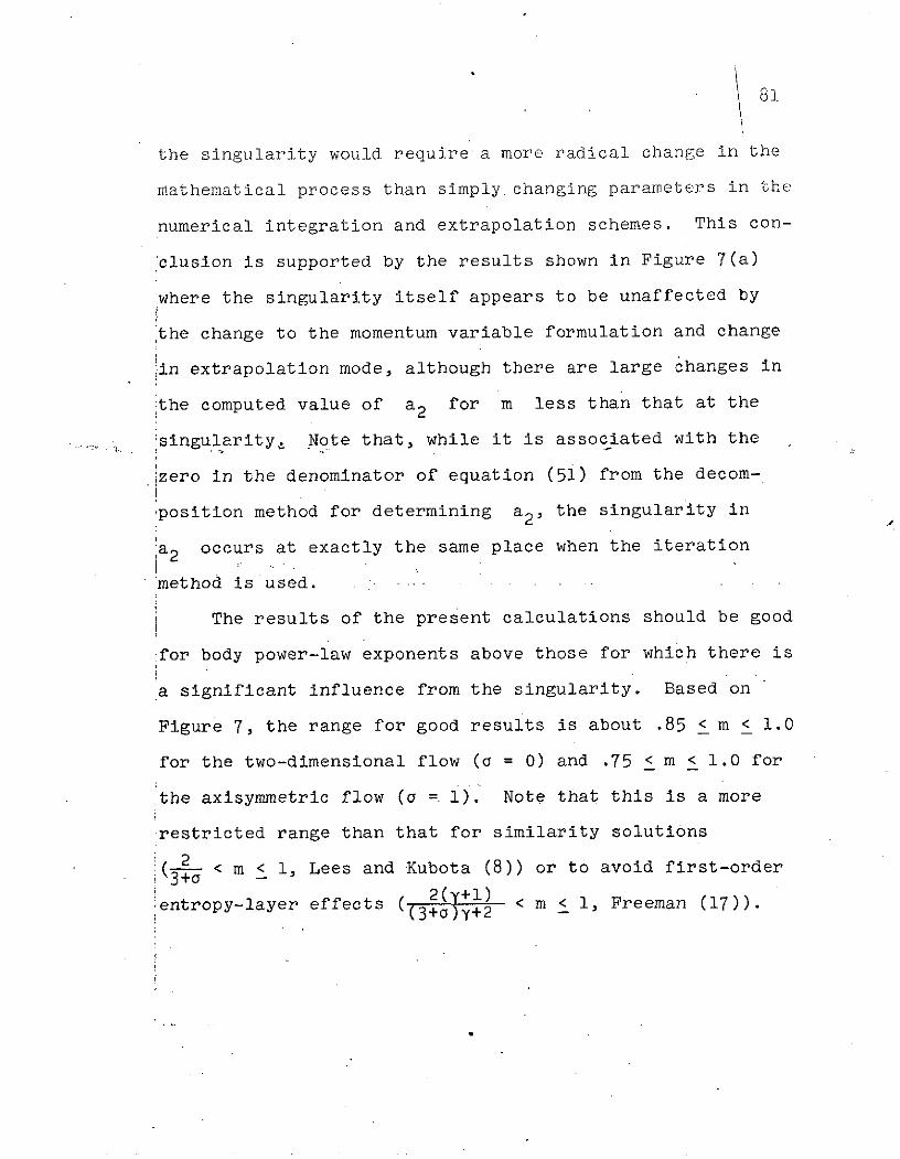
81

the singularity would require a more radical change in the

mathematical process than simply.changing parameters in the

numerical integration and extrapolation schemes. This con-

clusion is supported by the results shown in Figure 7(a)

where the singularity itself appears to be unaffected by

the change to the momentum variable formulation and change

!in extrapolation mode, although there are large changes in

ithe computed value of a2 for m less than that at the

singularity, Note that, while it is associated with the

izero in the denominator of equation (51) from the decom-

;position method for determining a2, the singularity in

a2 occurs at exactly the same place when the iteration

method is used.

The results of the present calculations should be good

:for body power-law exponents above those for which there is

a significant influence from the singularity. Based on

Figure 7, the range for good results is about .85 < m < 1.0

for the two-dimensional flow (a = 0) and .75 < m < 1.0 for

the axisymmetric flow (a =. i). Note that this is a more

restricted range than that for similarity solutions

< m < 1, Lees and Kubota (8)) or to avoid first-orderS3+e

entropy-layer effects ( 2(y+) < m < 1, Freeman (17)).(3+a)y+2-

22

C. Order-62 Func.tions

The order-62 similarity functions F2 ' 2 , u2' and P2

from the momentum-variable formulation, computed for axisym-

metric flow (a = 1) using iteration, are shown in Figure 8.

iThese functions are seen to have some differences in behavior

from the zeroth-order functions-described in Section IV-A.

iThe most obvious difference is that the curves describing

;these functions do not all emanate from a single point at

n = 1. The variation at r = 1 is-due to the variation of

the .boundary conditions at the shock with the body power-law

;m and to the transfer of the boundary conditions from the

shock to .n = i. As was noted Section B of Chapter III, the

2,values of these order-6 functions at the body surface were

found using a linear extrapolation from the last computed

,point of the numerical integration. The range of the

extrapolation was less than .00002 in n for all the cases

shown except for m = 1.0, for which the extrapolation was

made over an n distance of less than .001.

The order-62 similarity functions F2' 2' v2 and ¢2

from the velocity variable formulation and using the cubic.

extrapolation to obtain the surface values are shown in

Figure 9 for axisymmetric flow (a = 1). The results shown

1were obtained using the decomposition technique for calculat-

ing the shock displacement constant a2 (equations (48) -

(52)), but essentially identical results were also obtained

83

0

-. 1

-.2

-. 3

0.75

F2 .

Body surface values

0.95

-.-

m= 1.00

-1.0 I I I I.75 .80 .85 .90 .95 1.00

(a) Pressure function, F2 (r).

Figure 8. Order-6 2 Similarity Functions from the Momentum-Variable Formulation for Axisymmetric Flow (a = 1).

84

18

16-

14i

12-

10-

2 8-

6- 0.75

0.80

2 -0.85

0.90

0.950 - m= 1.00

-2 I I I.75 .80 .85 .90 .95 1.00

(b) Density function, '2(r),


12

10-

8

6-

0.75

V 2 \

0-0.80

-2- 0.85

0.90

0.95

-6 = 1.006

-8 i I I I.75 .80 .85 .90 .95 1.00

(c) Longitudinal momentum function, u2 ().-


86

12

10-

8-

6-

Li-

0.75F2 2

0-0.80

-2- 0.85

0.90

-4- 0.95

m = 1.00

-6

-8 I I I.75 .80 .85 .30 .95 1.00

(d) Lateral momentum function, p2 (n).


87

0

-.1

0.75

F2 -.5 0.80

Body surface valueO.85

0.90

0.95-. 7

m= 1.00

-. 8

-. 9

-1.0 I I I.75 .80 .85 .30 .95 1.00

(a) Pressure function, F2(T).

Figure 9. Order-62 Similarity Functions from the Velocity-Variable Formulation for Axisymmetric Flow (a = 1).

88

18

16

12-

10-

~ 8-

6 - 0.75

0.80

2 - 0.85

0.90

0.950 - m= 1.00

-2I I.75 .80 .85 .90 .95 1.00

(b) Density function, P2kq).


89

2.0

1.8

1.6

1.Lt

1.2

v, 1 .0 o

o2-0 9

.6

.2

0.75 .80 .85 .90 .95 1.00

(c) Longitudinal velocity function; v2().


0

-. 2

-. 6

-. 8- m.

2 -1.0 -2 -1.2

-1 .2 - 10.90

-1 .4 -

tio 0i

-1.8 0

-2.0 I I I I.75 .80 .85 .90 .95 1.00

(d) Lateral velocity function, 2 ().


91

using iteration. The two functions F2 and $2, which are

the same in both the velocity-variable and momentum-variably

formulations, are practically the same in Figure 9 as in

Figure 8. However, for power-law exponents less than those

:shown there are differences which become large as m de-

'creases, corresponding to the behavior of the constant a2

'(Figure 7).

The same comparison between methods of computing the body

!surface values of the order-6 2 similarity functions that was

made above for the axisymmetric bodies can be made for the

two-dimensional bodies (a = 0). The momentum-variable

similarity functions for these bodies computed using the

Alinear extrapolation technique are shown in Figure 10. The

:velocity-variable similarity functions computed using the

,cubic extrapolation technique are shown in Figure 11. These

two sets of functions exhibit the same type of agreement as

the functions for axisymmetric bodies (Figures 8 and 9).

All of the order-62 velocity and momentum functions

show singular behavior at the body surface for m < 1. It

was in anticipation of such behavior for v that the

momentum-variable formulation was undertaken (Section II-D).

'While the reformulation was successful in avoiding the un-

limited growth of v at the body, it did not avoid the same

,type of behavior by the order-62 functions. Because of this

!failure to eliminate the singularities and because it does

92

0

-. 1

-. 2

F2 -. 5 - Body surface

values-m= 1.00

-. 6 0.95

0.90-. 7

0.85

-. 8

-. 9-

-1.0 I I I I.75 .80 .85 .90 .95 1.00

(a) Pressure function, F2 (n).

Figure 10. Order-6 2 similarity fuhctions from the velocity-variable formulation for two-dimensional flow(a = 0).

93

8

7

6

S5-

0.85

3-

2

0.90

1

0.95

0- m= 1.00

-1

-2 I I I I.75 .80 .85 .30 .95 1.00

17

(b) Density function, q2(n).


94

2.0

1.8-

1.6-0.85

1. -

1 2 - 0.90

12 .0-

0.95

m= 1.00

14-

-2

10 I I I I.75 .80 .85 .30 .85 1.00

(c) Longitudinal velocity function, v2(n).


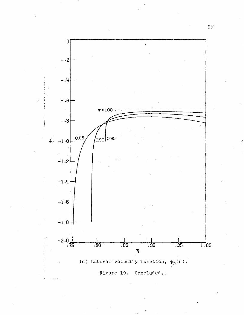
95

0

-. 6

m= 1.00

-. 8

k2 -1 .0 0.85 090 95

-1.2

-1.6

-1.8

-2.0 I I I 1.75 .80 .85 .80 .5 1.00

(d) Lateral velocity function, 42 (r).

Figure 10. Concluded.,

96

0

-. 1

-. 2

-. 3

z -.5 Body surface

values m= 1.00

0.95

0.90

-.6-

0.85-. 8

-. 9

-1.o I 0 I I.75 .80 .85 .90 .95 1.00

(a) Pressure function, F2(r).

Figure 11. Order 62 similarity functions from the momentum-variable formulation for two-dimensional flow(a = 0).

- 97

7

6 -

5-

q41.3-

2 - 0.90

1-0.95

0 m=1.00

-1

-2 I I I I.75 .80 .85 .0 .95 1 .oo

77

(b) Density functi.on, 2 (n).


98

2

1- 0.85

0

-1

0.90

u2 -3-

0.95

-5 - m= 1.00-S

-6

-7

-8 I I I.75 .80 .85 .90 .95 1.00

(c) Longitudinal momentum function, u 2(r)*


99

2

1-

0.85

0-

-1

0.90

-2

/2 -3 -0.95

-4- m= 1.00

-5-

-6-

-7-

-8 I I I I.75 .80 .85 .90 .95 1.00

97

(d) Lateral momentum function, P2 (I).


100

2not improve on the results of the order-6 velocity-variable

formulation in either quality or range of application, the

momentum-variable formulation of the flow equations has very

little advantage over the more conventional velocity-variable

formulation. It has, however, provided a useful check of

the numerical results.

The singularity at the body surface is thought to be an

entropy layer effect caused by the blunt nose of the body

for m < 1. The effect is confined to a very narrow region

since the very high curvature in the nose area (infinite at

i = 0) reduces the body slope rapidly. For example, when

m = .80 and 6 = .5, the slope decreases from infinite to

less than 1.0 before x/~ .006.

As noted previously, Mirels (10, 16) recognized the

singularity at the body surface and avoided calculating the

longitudinal velocity function, which exhibits the singular

behavior. In addition, Mirels (10) developed an approximate

analytic solution which is valid at the surface and used it

to obtain surface values of the zeroth-order functions (see

Appendix, Section A). The attempt to extend the approximate

analytic solution to order 62 is also discussed in the

Appendix.

Van Dyke (29, p. 185) notes the same singular behavior

in a small disturbance solution at the surface for hypersonic

flow over a blunted wedge and observes that it occurs because

101

the zero-order solution "is not a valid first approximation

in the entropy layer." He uses the method of matched asymp-

totic expansions to obtain a uniformly valid analytic solu-

tion for the blunted wedge. Adaptation of that method to

the similarity solution problem for power-law bodies

probably would extend the solutions to the body surface; but,

the application is not straightforward since the similar

solutions are not analytic and therefore do not give the

order of the singularities which occur.

The effect of the singularity at the body surface,

then, is to make the order-6 2 solution inapplicable at the

body surface except for the particular case m = 1, for

which the body does not have a blunt nose. But, the

singularity should not affect the solution away from the

surface, where the similarity functions are of order unity,

so long as the constant a2 is correctly determined.

Furthermore, the behavior of the order-6 2 similarity

function for the pressure (F2) is quite regular all the

way to the surface. Thus, the body surface pressure can

be calculated using this function; however, the results

must be suspect until checked against experiment or more

exact results.

102

It is because of the singular behavior of the similarity

functions that the numerical integration cannot proceed all

the way to the body surface. Neither do the extrapolations

follow the singular functions in giving values at the sur-

:face; so, the calculated surface values of these functions

do not represent the actual values of the singular functions,

which go to either plus or minus infinity at the surface.

To the extent that they are useful for determining the value

pf a2 , the extrapolations can be considered as providing

a limiting process for this constant.

D. Region of Validity of the Solutions

Three basic assumptions were required in order to obtain

the hypersonic similarity solutions for power-law bodies:

:(1) the body is slender enough that terms of order 6 are

negligible compared to unity; (2) the shock wave about the

body is strong enough that terms of order E 1 l/62 M2 are

negligible compared to unity; and (3) the Mach number is large

compared to unity. (The second of these can be relaxed to

E << 1 if the first-order solution in E is applied.)

However, even when these three assumptions are met overall

;for a particular power-law body, they generally are not all

met in particular local regions.

The first assumption, 6 << i, is obviously violated

in the nose region of all blunt bodies, such as the power-law

103

bodies for m < 1. Thus, the similarity solutions cannot be

expected to apply at the nose of these bodies. But, the

order- 2 solutions should be particularly useful in provid-

ing an improved solution a moderate distance behind the nose.

A's mentioned in the previous section, the violation of the

'slender body assumption by the blunt nose is also the cause

of the singularities in the order-6 2 functions at the

body surface. Therefore, because the first assumption is

2violated at the nose, the order-62 solution does not apply

.at the body surface.

The strong shock assumption, c << 1, is violated wherever

-1Ithe shock wave angle approaches the Mach angle, sin (1/M.).

Unless the Mach number is extremely large, the shock wave

will become weak far downstream from the nose of the body,

and the similarity solutions will not apply in that region.

The similarity solutions apply, then, in an intermediate

region from behind the nose to somewhere in the vicinity of

,the base of the body, and, in the case of the order-6 2

solution, only outside of the singularity at the body sur-

Iface. The boundaries of this region depend on the Mach number

and on the power-law exponent and slenderness of the body.

Decreasing the Mach number or increasing the slenderness of

the body tends to weaken the shock; decreasing the power-law

exponent increases the nose bluntness but weakens the shock

:at the rear of the body. In any case, the boundaries of the

104

region in which the solutions apply are not sharply defined.

They depend on the accuracy required in the results of each

particular problem and must be ultimately determined by

'comparison with experimental results.

E. Comparison With Other Solutions

The only exact solutions available for comparison with the

:similarity solutions are those for flow over cones and

wedges, corresponding to a power-law exponent of m = 1.

Since the zeroth-order and order-62 similarity solutions do

Inot contain any Mach number dependence, the most appropriate

;comparison is at the hypersonic limit, Ms + . (To include

iMach number effects the order-E solution would have to be

,used also.) Results from the similarity solutions, in terms

iof the physical flow variables, are compared in Figure 12

with the exact solutions for flow over a range of wedge

-angles at infinite Mach number. This flow, of course, is

uniform behind the straight oblique shock wave, as indicated

by the solutions for m = 1 in Figure 4, pages 66 - 69,

and Figures 10 and 11, pages 92 - 99. In Figure 13, results

from the similarity solutions are compared with the exact

solutions for flow over circular cones., Parts (a) of

,Figures 12 and 13 show the variation of the shock wave angle

iwith the body surface angle, and include exact results from

references 24 and 25 for several Mach numbers in addition to

60[. 105

56

Theory

52- Oblique shock(exoct)-- , Zero-order similorily}

Order-8' similority m=1

48

44

40-

36-/

32 -

28

24--

20

16 -

12

8-

4 -

4 .t .2 .3 .4 .5 .6 .7 .8 .9 1.0

0 4 8 12 16 20 24 28 32 36 .40

b ,deg

(a) Shock wave angle, 0s .

Figure 12. Comparison of Similarity Solution for m = 1with Exact Solution for Flow Over a Wedge at

OO

106

1.5

1.4

1.3 /

1.2

Theory

Oblique shock(exoct), M. co1.1 - - Zero-order similority) /

- Order-82 similoriy m=Newtonian

1.0 /

.9 /

.8 /

/ /

.7 -

.6

=..5 .3 .4 .5 .6 .7 .8 .9 10

4 8 16 20 24 28 .32 36 40

8b,deg

(b) Pressure,.p/qm /

Figure 12. Continued.Figure 12. Continued.

16

aj 12

t 8

-CC 4

- 12

.OO

.96-

.92

0 0

.88

0) Theory

.84 Oblique shock(exoct), M.= aD

,-- Zero-order similarity m3-- Order-S' similority

U .80

.76

.72 - 8.l .2 .3 .4 .5 .6 .7 .8 .9 1.0

II I I I I

0 4 8 12 16 20 24 28 32 36 400b ,deg

(c) Magnitude and direction of the velocity vector.


1.0 --

.9

ID

.6 -

oTheory

.5- Oblique shock(exoct), M,= o

- Zero-order similority \Order-8' similority m =1

0-J

.4

.3 -

E

.7

a21 -

47 .5

00

Fiure 12. Concluded.

.1

0 4 8 12 16 20 24 28 32 36 40O,deg

'(d) Velocity components.


i09

56-

52

48-

44 -M, 1.5

40-

36-

28

24

20

16

12- Theory

Conicol shock (exact)Zero-order similaorityOrder-8' similarity m=1

12

4- 24

8=.1 .2 .3 .4 .5 .6 .7 .8 .9

0 4 8 12 16 20 24 28 32 36 40

b ,deg

(a) Shock wave angle.

Figure 13. Comparison of Similarity Solution for m = 1with Exact Solutions fbr Flow Over a CircularCone at M0 = .

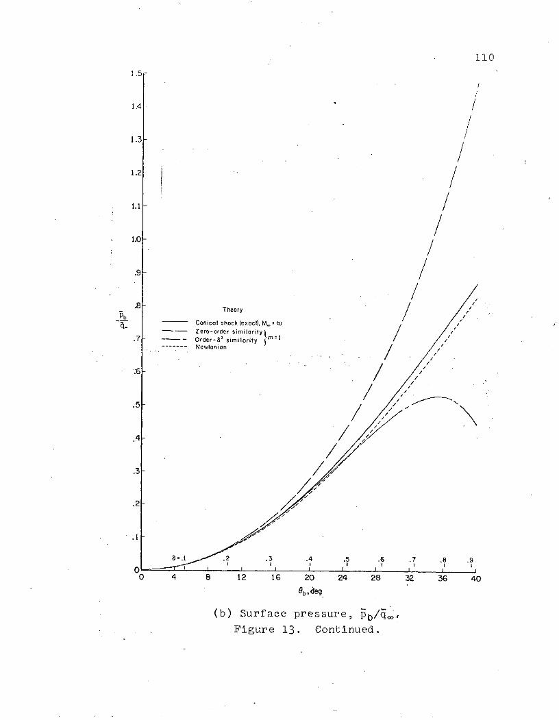
110

.5

1.4-

1.3 i

1.2 /1.1 /

1.0

.9

-.8b .8Theory

Conical shock (exoct). M, coZero-order similarity /.7 -- Order-S' similarityNewtonian

.5 -

.2-

.4

. .2 .3 .4 .5 .6 .7 .8 .9SI I I I

0 4 8 12 16 20 24 28 32 36 40

Ob, deg

(b) Surface pressure, pb/qc,


c 8

c -4

d 4

0

C -

00

1.00

.96

". .84 Theory

-c4-

.7

.=.1 .2 .3 .4 .5 .6 .7 .8 .9

(D)

0 4 8 12 16 20 24 28 32 36 40

8,,deg

(c) Magnitude and direction of the velocityvector at the body surface.


112

1.0

.9

I:,.8

C:

0

C0

o .7

2 .5 Theory

o Conical shock (exact), M.= oDJ- Zero-order similarity '

.4 - Order-8' similority m=1

.3-

.7

.

0

4 8 2 16 20 24 28 32 6 40

0

00 4 8 12 18 20 24 28 32 36 40

8b,deg

(d) Surface velocity components.


113

M = . The similarity results are found fromtan e,

tan s =' = 6R', where 6 1- _ and R' iss 2rb,f 11 b

found from equation (7) with m = 1.- The other parts of

the figures show the variations with the body surface angle

pf the pressure coefficient p/q , the velocity

-2 -2/u = -2 + v2 /u , and the velocity components u/u,

and v/u in the uniform flow behind the shock wave,(Figure

,12) and at the body surface (Figure 13). These similarity

results are found from equations (8) with m = 1. The exact

results are found from the oblique shock relations in the

,two-dimensional case and from the charts of reference 24 in

the axisymmetric case.

These Figures show that for m = 1 the zeroth-order

Isimilarity solution agrees well with the exact solution for

body surface angles up to about 0b = 120, while the order-62

solution agrees well up to body angles of about 6b = 200

As can be seen at the bottom of the Figures, these cone or

Iwedge angles correspond to slenderness parameter values of

about 6 g .2 and 6 z .4. The similarity results for the

magnitude of the velocity show good agreement for even

larger body angles (Figures 12(c) and 13(c)). Since the

,error in the velocity components is larger (Figures 12(d)

tand 13(d)), it must come largely from error in predicting

the direction of the velocity vector. This error in

direction is shown in theupper part of Figures 12(c) and

2 and -13(c), where it is compared to the curves 6 ab and -6 0 b

These curves represent the order of error expected from

neglecting terms of order 2 and of order 6 , respectively.

The error actually occurring is seen to be very close to

that which was expected. It should be noted that this error

in the direction of the velocity vector corresponds to an

'error in satisfying the boundary condition that there should

be no flow through the body surface. That is, the velocity

'component normal to the surface, = sin tan-( ) -

should be zero (Figure 3, p. 30). Figures 12(c) and 13(c)

Ishow that this boundary condition is satisfied to order 62

by the order-62 similarity solution for m = 1.

In Parts (b) of Figures 12 and 13, the pressure coeffi-

Cients are compared also with the Newtonian prediction:

p/q = 2 sin2 0b . The Newtonian prediction is much more

;accurate for the conical flows (Figure 13(b)) than for the

,wedge flows (Figure 12(b)); however, even in the conical

case the order-6 2 similarity solution is closer to the exact

isolution for moderately small values of the similarity

parameter, i.e. 6 < 0.5.

In Figure 14, the variation of the flow variables from

the shock to the body is shown for three values of the

power-law exponent, m = .75, .85 and 1.0. The pressure,

density and velocity components, calculated from the axisym-

2,metric zeroth-order and order-6 similarity solutions, are

shown at x/1 = .5 for a similarity parameter value of

115

6 = 0.4. The exact solution for a cone at Mach 20 with

0b = 200 (reference 25) is also shown in Figure 1 4(a) for

comparison with the case m = 1.0. Although the conical

bodies are not the same (6 = 200 corresponds to 6 = .3978),b

12the order- 62 similarity results agree well with the Mach 20

solution shown for all the variables except the density. As

ican be seen by the symbols representing the exact solution

for Me + O at the shock wave, the density is the only one

iof the flow variables that is much affected by the difference

Ibetween M = 20 and M + '. The similarity solutions for

:the density agree exactly with the. infinite Mach number

tsolution at the shock. The order-62 solution for the other

,variables differ from the exact, infinite-Mach number solu-

ition at the shock by amounts which are of order 6 , as

iexpected from the approximation to the oblique shock relations

'used (equations (4)). On the other.hand, the zeroth-order

similarity solution is not accurate for a cone of this thick-

;ness; it is off by an amount of order 62, which is 16% for

6 = .4. Note that the zeroth-order results stop at n = 1,

which is the zeroth-order shock wave location. The order-62

results at the shock are given by equations (15); the

,integrated solution begins at n = 1, with the results in

the region 1< n < ns given by the Taylor series expansion

,as discussed in Section III-C.

7 - _16

6-

P

5

.92-

.88

.84

-- Exact, M= 20., b=20*

.80- Zero-order similarity solutionOrder-8' similority solution

o Newtonion. Tongent-cone. (exocl),M, ,

.40 - o Exact solution of shock, M.= O

.20 -

.16

Body / . Shock

0 .1 .2 .3 .4 .5 .6 .7 .8 .9 1.0r-f b

R-r(a) Power-law exponent m = 1.0 (conical body).

Figure 14. Variation of Flow Variables from Body to Shock atx/I = 0.5 for Axisymmetric Flow with 6 = 0.4.

117

6--

5-

% 4

3

2

.92-

.88 -. _----

.84 -Zero-order similority solutionOrder-8' similarity solution

O Newtonion.80 w Tongent -cone, M.= c

.36

.32 --

.28 - - ----- -

.24

S.20

.16

Body * tp.0 Shock

0 .1 .2 .3 .4 .5 .6 .7 .8 .9 1.0r- rb

R-rb

(b) Power-law exponent m = 0.85.


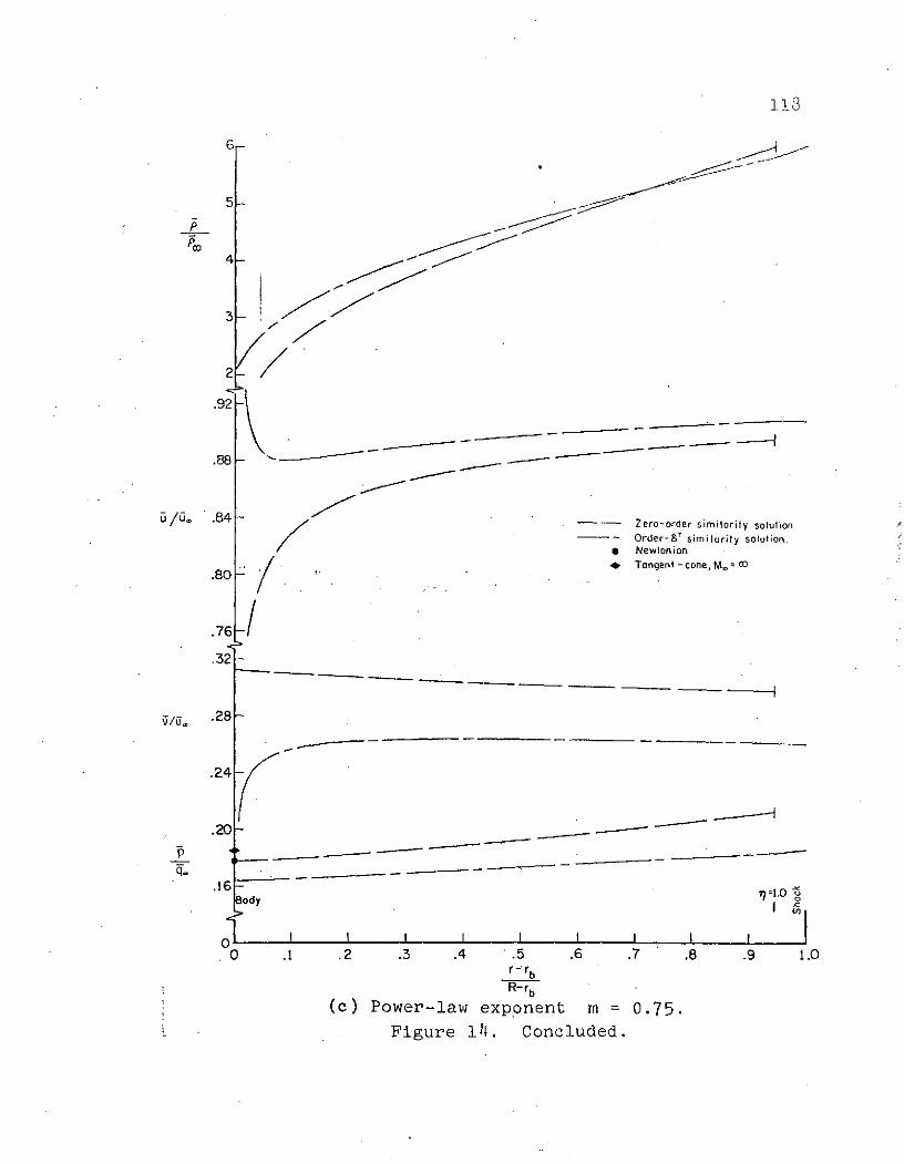
6-

5-

P.L

4 -

2.92

.88-

/O. .84- - Zero-order similarity solutionOrder-a8 similarity solution.

* Newtonian

.80 . Tangent -cone, M. 0

.76 -/

.32-

.28

.24 -

.20

q- - - - ---------

.16 77=10Body O

0 .1 .2 .3 .4 .5 .6 .7 .8 .9 1.0r -rbR-rb

(c) Power-law exponent m = 0.75.Figure 14. Concluded.

For body power-law exponents other than m = 1 there

is no exact solution available for comparison with the order-

62 solution. However, there are some simple empirical methods

for estimating the pressure on general bodies. Two of these

methods will be used for comparisons. One is the Newtonian

2law C = 2 sin 0b. As discussed by Hayes and Probstein (1),

Cp

:it corresponds to the limits y + 1.0 and M. c; but, it

iis widely used for more general hypersonic flows in this or

'modified form. The other empirical prediction is the

,tangent-cone method, which takes as the pressureat any point

on a body the pressure on the cone having the same surface

angle as the body point. This method also is most accurate

~or -M- 00, since then the shock layer is very thin with

ilittle pressure change across it. Hayes and Probstein (1)

tgive a thorough discussion of these two methods and their

limitations. Only one limitation will be mentioned here:

these methods give only the body surface pressure and are

not complete flow field solutions, as are the similarity

!solutions.

The calculated flow fields for bodies having m = .85

and m = .75 are shown in Figures 1 4(b) and (c). In these

cases the order-62 solution is again a major correction to

'the zeroth-order solution. However, the singularities

2in some of the order-6 similarity functions show up here

at the body surface. Because of the singularities, the

12 0

order-62 values of the density and the velocity components

are probably unrealistic close to the surface. Fortunately,

the pressure is well behaved all the way to the body surface,

so that surface pressure coefficients can be calculated.

The surface pressures calculated from the similar

solutions are seen in Figures 14(a), (b) and (c) to agree

fairly well with the empirical predictions of the Newtonian

iand tangent-cone methods. However, as m goes from 1.0 to

2:0.85 to 0.75 the order-6 similarity solution pressure

drops faster than the tangent-cone and Newtonian pressures,

;so that the agreement becomes progressively worse. Whether

the similarity solution or the empirical methods give a

+better representation of the actual pressure changes with body

power law must be determined by comparison with experiment

as in the following section.

F. Comparison with Experimental Results

There is only a limited amount of useful experimental

data on the hypersonic flow fields about power-law bodies.

This data consists mainly of measured shock wave shapes and

surface pressure distributions for 3/4- and 2/3-power bodies

of a few different fineness ratios. In this section the

similarity solution predictions for shock wave shape and

surface pressure for axisymmetric bodies with power-law

exponent of m = 0.75 will be compared with the experimental

121

results of Kubota (9) and Peckham (19). No comparison is

made with results for smaller power-law exponents since

valid order-6 2 similarity solutions were not obtained in

those cases. Also, no comparisons are made with experimen-

tal total drag measurements (e.g. those of reference 22)

because of the uncertainty in calculating the skin friction

contribution.

Shock shape. Because the shock displacement constant

a is so small, the order-6 2 shock wave shape is only

,slightly different from the zeroth-order shape, an example

;of which is shown in Figure 1, page 13. For example,

a= .0582 when m = .75 in axisymmetric flow (Figure 7,

page 78, a = i); thus, even for 6 = 0.4, the order-62

:term in equation (7) for the shock shape R/I amounts to

;only about .003 at the base of the body (x/. = 1.0). There-

fore the order-6 2 shock wave shape cannot be expected to be

much closer to the experimentally measured shock shape than

is the zeroth-order shape.

The zeroth-order and order-6 2 shock wave shape predic-

tions are compared to the shock shape data for m = .75

from references 9 and 19 in Figure 15. These data are pre-

sented in the correlation form used by Peckham (19) after a

suggestion by Hornung (26).

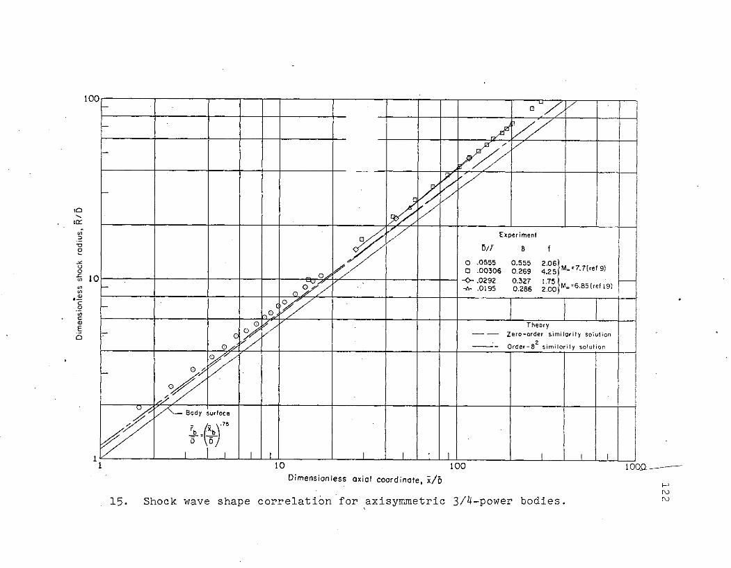
100

V) ExperimentU,

0 .0555 0.555 2.06

0 n .00306 0.269 4.25 M==77(refg)

5 10 0 .0292 0.327 1.75M=85(ref 191 ) -6- .0195 0.286 2.00M

L o Po, _ _ T heory

0 - - Zero-order similarity solution

O /_ -- Order-82

similority solution

Body surface

7b "b)'

1 10 100 1 00Q --Dimensionless axial coordinate, i/5

15 Shock wave shape correlation for axisymmetric 3/-power bodies.15. Shock wave shape correlation for axisymmetric 3/4-power bodies. ,

123

The experimental data for the .shock shapes are seen to

correlate well with one another but to fall somewhat above

the similarity solution predictions. This difference between

experiment and theory is largely due to the difference in

Mach numbers (6.85 and 7.7 for experiment, Mc - for

theory). It is comparable to the shift in shock location

with Mach number for cones (Figure 13(a), page 109).

The experimental results correlate together because their

Mach numbers are relatively close. An additional cause for

!the difference between the experiment and theory is the out-

ward displacement of the flow by the growth of the viscous

boundary layer on the experimental bodies.

-- --The effect of the order-6 2 term in the similarity

!solution for the shock wave shape is seen in Figure 15 to

increase as x/D decreases. This is expected since small

values of x/D correspond either to small values of x/

or to large values of D/, that is, either to points near

the nose of the body where the slope is larger or to bodies

which are less slender and thus have larger 6 values. Note

that the agreement of experiment with theory is better in

!this region of smaller x/D values, as would be expected

since the shock location is closer to that for infinite

Mach number for larger body slopes. The slope of Kubota's

-data for D/Z = .0555 (circles in Figure 15) agrees very

iwell with the slope of the order-6 2 similarity solution;

124

this agreement in the slope on a log-log plot indicates good

agreement of the power-law exponent of the physical shock

wave shape.

Additional shock wave shape data from hypersonic flows

over power-law bodies is presented by Freeman, Cash and

;Bedder (20) (m = .75, M = 8.8) and by Beaver (21) (m = .85,

M = 7.0). Althoi~gh they apparently correlate in the same

way as the data in Figure 15, these data are not presented

here because they fall in ranges of very large x/D values,

!for which the order-6 2 term of the shock wave shape equation

'is negligible. For these large x/D values the strong shock

assumption, corresponding to c l/(MS)2 2<< 1, may not be

satisfied. (See Section II-B). For-example, c .36 for

the 3/4-power bodies of reference 20. Thus the first-order

.solution in E would have to be applied to obtain useful

results.

Pressure distribution. The pressure distributions

obtained by Kubota (9) and Peckham (19) are shown in Figure

16 for the same 3/4-power bodies as used for the shock

wave shapes in Figure 15. In addition to the zeroth-order

and order-62 similarity solution predictions, the two

,empirical pressure distributions are presented. As seen in

'Figure 16, the similarity solutions as well as the two

;empirical methods give pressure distributions in good agree-

ment with the experimental data for the three bodies having

STheory

Tongent -cone

Zero-order simniiirity.5 - \- - Order-8' similoriy

m =i-- - Newfonion

Experiment

-- 0 8=0.555 f 1.03 M 7.7(ref9 )

.3 --

.2-

..

.4

01

.30 8= 0.286, f 2.00, M.6.85(ref 19)

.2

0 I I I I I I I I0 .1 .2 .3 .4 .5 .6 .7 .8 .9 1.0

i/l

Figure 16. Comparison of similarity solutions with experimentalpressure distributions; m = .75 (Theory is for samevalues of 6 as experiment; tangent-cone for sameMach number).

126

fineness ratios f k / 2rb(Q) of about two. For these cases

the order-62 similarity solution is very nearly the same as

the zeroth-order solution except at the front of the body.

The Newtonian prediction falls slightly higher than the

similarity solutions back of the nose region, but curves

representing these three methods are below the data points.

iSince at hypersonic speeds the viscous boundary layer

'tends to displace the flow outward, raising the pressure

,above that which would occur for inviscid flow, the theore-

itical inviscid pressure levels are expected to fall slightly

below those actually measured. For example, by applying a

iboundary layer displacement correction to the zeroth-order

Tsimilarity solution for the pressure on his fineness ratio

2.13 body, Kubota (9) obtained excellent agreement with his

experimental data (squares in Figure 16). Since the tangent-

cone pressure distribution falls slightly above the experi-

mental data for the three higher-fineness-ratio bodies, the

.other methods are somewhat preferable for these cases.

It is in the case of the body having a fineness ratio

of nearly one, however, that a real difference between the

methods appears. In particular, the difference between the

,zeroth-order and order-62 pressure distributions becomes

substantial. The zeroth-order result lies above the

experimental data by an amount which increases rapidly

,toward the front of the body. On the other hand, the order-62

127

result lies below the data by an amount which, for most of

the body, is only moderately larger than that for the finer

bodies. This amount is on the order of the expected

boundary layer displacement effect. It is only at the front

2of the body that the order-6 result begins to diverge

markedly from the experimental pressure distribution. Since

the value of the slenderness parameter is 6 = 0.555 for

this case*, it is not surprising that the order-6 2 similari-

ty solution should begin to fail as the body surface angle

iincreases at the front of the body. This is about the same

.value of 6 as the limit for good-results in the wedge

and cone cases (Figures 12 and 13, pages 105-112). The

Newtonian method gives excellent agreement with the experi-

mental data in this case, but this must be somewhat fortuitous

iin that no correction was made to account for the boundary

'layer displacement effect. The tangent-cone method again

lies somewhat above the experimental data.

*Kubota's (9) value 6 = .485 shown with his data correspondsto 6 b = .485 as used herein.

CHAPTER V. CONCLUSIONS

Beginning with the equations for conservation of mass,

conservation of momentum, and conservation of energy for

the inviscid, two-dimensional or axisymmetric adiabatic flow

.of an ideal gas, similarity solutions have been found which

give the flow field to order-62 about power-law bodies in

the hypersonic limit M -* , where 6 is a body slenderness

'parameter. On the basis of this investigation the following

,conclusions can be made:

1. The order-62 solutions are independent of the

slenderness parameter 6. Thus the functions expressing

the solutions are universal in that they apply for all values

of 6 for which 6 << 1. The relations between these

similarity functions and the physical flow variables are

Irelatively simple.

2. For the purpose of obtaining the similarity solu-

tions the flow equations can be formulated in terms of the

.longitudinal and lateral momenta as basic variables instead

of the corresponding velocity components, and the similarity

!functions can be obtained. However, the expected advantage

lof avoiding singular behavior of the equations at the body

!surface do.es not materialize.

3. In the present formulations the value of a2 , the

shock displacement constant in the order-6 2 solution, goes

128

i 129

through plus and minus infinity at about m = .817 in the

two-dimensional case and m = .653 in the axisymmetric

case, where m is the body power-law exponent. Because the

singularity does not correspond to actual flow conditions

it must arise through the mathematical development. Since

the singularity was not removed by any of the variations in

solution procedure tried, the present results are limited to

a range judged relatively free of effects from the singularity

'(.85 < m < 1.0 for two-dimensional flow, .75 < m < 1.0 for

axisymmetric flow).

4. In comparisons with the exact solutions for inviscid

:flow over wedges and circular cones, the order-62 similarity

,results give excellent agreement for 6 less than about .4,

corresponding to wedge or cone angles up to about 200. Over

an even larger range,the order-62 surface pressure predic-

tions were superior to the Newtonian pressure law. The

order-6 2 results were a significant improvement over the

zeroth-order results for body angles greater than about 120

5. In comparisons with experimental shock wave shapes

and surface pressure distributions for 3/4-power axisymmetric

bodies,the order-62 similarity solutions gave good results,

:considering that Mach number and boundary layer displacement

.effects are not included in the theory. For body fineness

ratios near two, the effects of the order-6 2 terms are

significant only very near the body nose, whereas for a

130

fineness ratio near unity the order-62 terms had a large

effect over almost the entire body. These good results for

the surface pressure were obtained despite the singular

behavior of some other variables at the surface.

6. While the order-62 similarity solutions were

:developed for the hypersonic limit M_ ~, the derivation

ishows that they are compatible with the order-c solutions

2of Kubota (9) and Mirels (16), where c E /(M.6) . The

order-c solutions introduce Mach number effects.

7. While all present results were obtained for no

!flow through the body surface as a boundary condition, it

appears from the derivation that small amounts of blowing

or.suction through the wall could be easily accommodated.

8. It was noted that the correlation suggested by

,Hornung (26) for the shock wave shape and body pressure

distribution can be applied exactly to all of the flow

variables in the order-62 similarity solution form. This

finding suggests a method of correlating for future

.experimental data. The form of correlation also suggests

a possible refinement of the derivation of the order-62

similarity results, using the local body or shock wave slope

as the small parameter.

BIBLIOGRAPH.

1. Hayes, Wallace D.; and Probstein, Ronald F.: HypersonicFlow Theory. (Second edition). Academic Press,New York, 1966.

2. Taylor, G. I.: The Formulation of a Blast Wave by aVery Intense Explosion. Proc. Roy. Soc. London,Ser. A, Vol. 201, 1950, pp. 159-186.

3. Sakarai, Akira: On the Propagation and Structure of aBlast Wave, I. J. Phys. Soc. Japan, Vol. 8, no. 5,Sept. - Oct. 1953, pp. 662-669.

'4. Sakarai, Akira: On the Propagation and Structure of aBlast Wave, II. J. Phys. Soc. Japan, Vol, 9, no. 2,March - April 1954, pp. 256-266.

5. Hayes, W. D.: On Hypersonic Similitude. Quart. ofAppl. Math. Vol. 5, no. 1, April 1947, pp. 105-106.

6. Van Dyke, Milton, D.: A Study of Hypersonic Small-Disturbance Theory. NACA Rept. 1194., 1954.

7. Lees, L.: Inviscid Hypersonic Flow over Blunt NosedSlender Bodies. GALCIT Hypersonic Research Project,Memo No. 31, Feb. 1956.

8. Lees, Lester; and Kubota, Toshi: Inviscid HypersonicFlow over Blunt-Nosed Slender Bodies. J. Aero.Sci., Vol. 24, no. 3, March 1957, PP. 195-202.

9. Kubota, Toshi: Investigation of Flow around SimpleBodies in Hypersonic Flow GALCIT Hypersonic Res.Proj. Memo 40, June 25, 1957. Also, Inviscid Hyper-sonic Flow over Blunt-Nosed Slender Bodies. GALCITPublication No. 417, 1957.

10. Mirels, Harold: Approximate Analytical Solutions forHypersonic Flow over Slender Power Law Bodies. NASATR R-15, 1959.

11. Sedov, L. I.: On Certain Unsteady Motions of aCompressible Fluid. Prikl. Mat. Mekh., Vol. 9, 1945,pp. 293-311. Transl. no. T-57, The Rand Corp.,Santa Monica, Calif., 1956, cited by Hayes andProbstein (1).

131

132

12. Sedov, L. I.: Propagation of Strong Blast Waves.Prikl. Mat. Mekh., Vol. 10, 1946, pp. 241-250, citedby Hayes and Probstein (1).

13. Grodzovskii, G. L.: Certain Peculiarities of theFlow around Bodies at High Supersonic Velocities. Izv.Akad Nauk SSSR, Otd. Tekhn. Nauk, no. 6, 1957, PP.86-92.(Transl. by Morris D. Friedman, Inc.)

1:4. Chernyi, G. G.: Introduction to Hypersonic Flow. (R. F.Probstein, transl. and ed.) Academic Press, New York,1961.

15. Stanyakovich, K. P.: Unsteady Motion of Continuous Media.(J. G. Adashko, transl., and M. Holt, ed.), PergamonPress, New York, 1960.

16. Mirels, Harold: Hypersonic Flow over Slender Power-Lawand Related Bodies. Advances in Applied Mechanics,Vol. VII, Academic Press, New York, 1962, pp. 1-54, 317-19.

17. Freeman, N. C.: Asymptotic Solutions in Hypersonic Flow:An Approach to Second-Order Solutions of HypersonicSmall Disturbance Theory. Research Frontiers in Fluid

- Dynamics (R. J. Seeger and G. Temple, eds.) InterscienceMonographs and Texts in Physics and Astronomy, Vol. XV,John Wiley and Sons, 1965, pp. 284-307.

18. Sychev, V. V.: On the Theory of Hypersonic Flow overBlunt-Nosed Slender Bodies. Advances in AeronauticalScience, vol. 3 (Th. von Karman, chmn. ed. comm.),Macmillan Co., New York, 1962, pp. 87-102.

19. Peckham, D. H.: Measurements of Pressure Distributionand Shock-Wave Shape on Power-Law Bodies at a MachNumber of 6.85. Aeronautical Research Council C.P.871, April 1965.

20. Freeman, N. C., Cash, R. F., and Bedder, D.: AnExperimental Investigation of Asymptotic HypersonicFlows. J. Fluid Mech., Vol. 18, no, 3, March1964, pp. 379-384.

21. Beavers, G. S.: Shock Wave Shapes on HypersonicAxisymmetric Power-Law Bodies. AIAA J., Vol. 7,no. 10, Oct. 1969, pp. 2038-2040.

22. Spencer, Bernard, Jr., and Fox, Charles H., Jr.:Hypersonic Aerodynamic Performance of Minimum-Wave-Drag Bodies. NASA TR R-250, 1966.

23. Townsend, James C.: Hypersonic Aerodynamic Characteris-tics of a Family of Power-Law, Wing-Body Configurations.NASA TN D-7427, 1973.

24. Equations, Tables, and Charts for Compressible Flow.NACA Report 1135, 1953.

25. Sims, Joseph L.: Tables of Supersonic Flow aroundRight, Circular Cones at Zero Angle of Attack. NASASP-3004, 1964.

26. Hornung, H. G.: Inviscid Flow over Plane Power LawBodies. J. Fluid Mech., vol. 27, no. 2, Feb.1967, pp. 315-336.

27. Ashby, George C., Jr.: Longitudinal AerodynamicPerformance of a Series of Power-Law and MinimumDrag Bodies at Mach 6 and Several Reynolds Numbers.NASA TM X-2713, August 1974.

28. Ashby, George C., Jr.; and Harris, Julius, E.: Boundary-Layer Transition and Displacement-Thickness Effectson Zero-Lift Drag of a Series of Power-Law Bodies atMach 6.. NASA TN D-7723, September 1974.

29. Van Dyke, Milton: Perturbation Methods in FluidMechanics. Academic Press, New York, 1964.

30. Van Dyke, Milton: Extension, Analysis, and Improvementof Perturbation Series. Tenth Naval HydrodynamicsSymp., M.I.T., Cambridge, MA, June 27, 1974.

APPENDIX. ASYMPTOTIC SOLUTION IN TERMS OF

STREAM FUNCTIONS

A. Stream Function Formulation

This Appendix describes the development of an

asymptotically valid analytic solution to the flow equations

in terms of a similarity-function form of the stream func-

tion. The solution is basically the zeroth-order solution

of Mirels (10,16) with order-S 2 terms added. It is

Ideveloped from the velocity-variable formulation, which

Mirels used, but the results can be easily related to the

momentum-variable formulation also.

By definition, the stream function must satisfy the

'continuity equation (3), which may be rewritten

[p(l + 62u)] + (pv) + - 0.ax. ar r

If

p(l + 2 u) = a 3rr

and (Al)

a axr

then ' (x,r) is a stream function. It can be put into the

similarity form

134

1-35

0o(n) (1+o)m 24(,n) = (1+o)m + 6 2 B62(-) (A2)

where the zeroth-order term was given by Mirels (10) and

the constants B and j in the order-62 term are to be

determined by comparison with the similarity form of the

iflow variables (equation (8)). Putting the stream function

defining relations (Al) into similarity form (using

equation (A2) and the chain rule equations (9)):

8' 0'p(1+6 u) = + 6 B 2 gj-(l+o)mU a

(l+o)n n-and (A3)

n ] m -(l1-m) 2 m j-(+ompv [o - 6 B[ 2 ~-- E Tj-(l+m)0 l+C o a m 2 2 a

The comparable relations from equations (8), omitting the

'order-c terms, are

p(l + 62u)= o + 62( 2 "+V ~o)m2 -2(1-m) + 0(64)

and (A4)

pv = om - (l -m ) + 62 o2)m 3(1 -m ) + 0(6 4)pv -0 0 0 + ip0 2)m

Comparing these two sets of equations, the exponent in the

order-6 2 term of (A2) must be j = (3 + a)m - 2, and the

:similarity functions are related by the equations

o1 0 o.oo _ ( o(1+o)n 0 no l+o

BOE

mn

B (3+a)m-2o02 + 0o2 =2 o - m 2m

The boundary condition on the stream function similarity

functions are

0o(n b ) = 0, 6o(1) = 1

(A6)

e2(n b ) = 0, 02(1) = 1

Solving equations (A5) for the constant B and evaluating

'the similarity functions at n = 1, using equations (46)

and (A6), gives

2m2B - a2

y-l 2

so that

( o (l+G)m 2 2a2 2 (3+)m-2(,) 1+ - 6 y- l m (A7)

:In addition, equations (A5) can be.solved for

0' 0o o

0 0 0o0 = n- (l+) 0

oa [ 0 a2 (A8)

1+0 2a2 o 2 (3+a)m-2l+= 0 + i+o) o2 = o ' o y-1 ' m 2

o o

Or, conversely,

0 = (n - o)o

(A9)

(Y-l)m [(n-2 2a2[(3+o)m-2] 2 + o 2

As Mirels (10)-showed for the zeroth-order case, the

pressure can be related to the stream function by using the

energy equation. Defining an entropy function w E p/pY,

!the energy equation (3) in terms of the stream function

becomes

S0 aw o. (A10)ar ax ax ar

This has as a solution (to order 62)

2 -1 - 2 m-2(1-m) 2 2a2 02 4 -4(1-mS- (Y + 6 (l+a) - m (Ay+1 y+1 o -( l)

(All)

1.38

where the zeroth-order term is Mirels' zeroth-order solu-

tion (10) and the order-6 2 term was found by trial and

2(1-m)error. The parameter B is defined by (l+ ) and(l+o)m

'varies from zero to one as m varies from one to3+0'

the loweri limit for similarity solutions. The stream func-

,tion expression for the pressure can be found from the

,entropy function, since the expression for the density is

!already given by equations (A8). Thus the density and pressure

are

!pY 2Y[I + 2 2 -2(1-m) 4ip = o y m + 0(6 )]

0

- _+) - 62y( + 2(l+cr)' ] a ) + 0(6 )0 o -1 2 E)o

and

p = pYe

Y Y (8')Y2 -1 1 o 2 -2(1-m)(¥+ ) (- ) m (A 2)

S + 62 l(l+) a( 2 2 - 2(1-m) + 064

0o o

,On comparison with the similarity form of the normalized

pressure (equation (8)), this equation gives. the relations

139

(n) y+l y+) (l+) o()

0 y+1

and (A13)

F2 1 a2 e 0 o()]F(0 O

where, again, the zeroth-order function is Mirels'.

B. Zeroth-Order Approximate Solution

In reference 10, Mirels shows that, using equations (A8)

and (Al3) for 4o, o0, and F , the zeroth-order lateral

momentum equation (11) can be approximated for 00(n) <<.10

by

o 8 o a 0 (A14)0' y O no o

He also gives the solution to this approximation:

ao (n ) K o(nl+a 1+ )Y- (A15)0 0 b

where

Ko = [- (- - ) F o(nb ) (A16)

Mirels uses this solution to make an improved approximation

for the lateral momentum equation and an improved approximate

'solution

+l+ + Y-B _be (n) = Ko( - ) [1 + ] (A17).o b 2(2y- ) F 0(nb) o

Putting this second approximation back into equations (A8)

and (A13), he obtains the relations

1+0 1+ 1-a- on - n b n b

~-9 1 4 Y c - b [1 b o[ y - 2(2y-)F (nb

8 1-a- K (n l+ l+y-B + b (A08)S Y- 0 - b [ (2y-B)F (nb) (8)

y-B0 b

8 i-aF 0 F (nb) + 1- e

o 0 b 2nb 0

Using equations (A8) again,.he obtains from these relations:

1+onb n- B(n-0 o b n 1-0

(-) = 1 - - ( ) [1 + (-) 3y-B 2(2 y-B) F n

and (A19)

Fo(nb 2 ob( -o0 o

These relations are correct to the order of 82 and

therefore apply near the body surface, where o(n b ) = 0

(equation (A6)). Using (A15), terms of order 02 are less0

Y-

2 (61Ko) Ythan terms of order-6 when - < . At the

(l+o)ni

point where equations (A19) are used in the numerical

solution to determine the values of nb and Fo(nb), theb

integration has come so close to the body that

(6/K ) 0-b << Thus the error in relations (A17) tob b

(l+cr)b

(A19) at ithat point is much less than the order-6 error

of the equations being integrated, and the zeroth-order

;approximate solution for Fo' Co and o (relations (A18))

:may be used the rest of the way to the body surface.

The zeroth-order longitudinal momentum equation can be

used to obtain an approximate solution for vo(n) in the

:region near the body. Noting the implication for vo(ib)

from the body boundary conditions (equation (22)), a trial

solution is made in the form

Vo(n) = D o

(A20)F F'

v'(n) = D ( o 0o o Fo

Putting this into the longitudinal momentum equation (11)

.gives

F' F'D(n- To ) + r + 2(-)(D + 1) = 0.

Solving for D and substituting -from equations (A8) and

,(A13):

1 42

_ " 0+ o o £)

lDo 0 y 0° 1

D 0" 0' 0B + (y-l)( )n10' y0 nO'

o 0

But D is a constant, so an approximation must be made;

adopting Mirels'.first approximation (equation (A14)) reduces

D to - __-, so that the relation (A20) for v becomesy-1 l

(to order o, 0 << 1)

V' F() 2 _-vO (l) o 1+2 o (A21)o-1 o-) Y2 y+1 (+) (TY o

2C. Order-62 Functions

In principle, expressions (A8), (A13) and (A21) could be

put into the order-62 lateral momentum equation (13) to

obtain a first-order differential equation for the order-6 2

similarity stream function 82. However, the equation would

contain a very large number of terms and would require a

considerable amount of approximation to be made in order

to reduce it to a form for which a solution could be

obtained. The approximation process is complicated by the

facts that 6 occurs to non-integral powers and that many

terms contain 8, which itself takes on very small values

in the range of interest. Considering that the solution is

only to be applied in a very small region near the body

surface and that 02 is already of order-6 2 , the additional

14 3

accuracy which might be obtained probably does not justify

the additional effort required to produce an approximate

solution in this way. Instead, the simple linear extrapola-

tion techniques described in Section III.B are used to

carry the order-6 2 similarity functions the short distance

Ito the body surface.

for · inviscid,itwo-dimensional or axisymmetric adiabatic flow of an ideal gas, similarity...

Documents