for experts and combinatorial games - course web … experts and combinatorial games wouter m....
TRANSCRIPT
Second-order Quantile Methodsfor Experts and Combinatorial Games
Wouter M. Koolen Tim van Erven
Royal Holloway, Friday 28th August, 2015
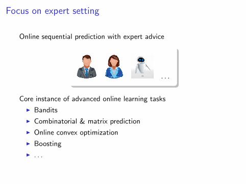
Focus on expert setting
Online sequential prediction with expert advice
. . .
Core instance of advanced online learning tasks
I Bandits
I Combinatorial & matrix prediction
I Online convex optimization
I Boosting
I . . .
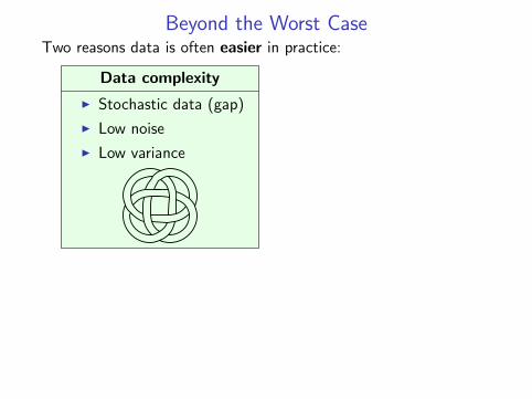
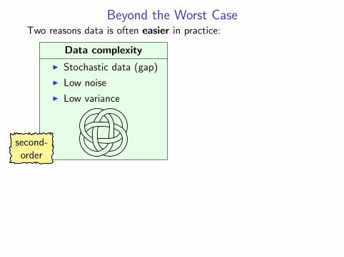
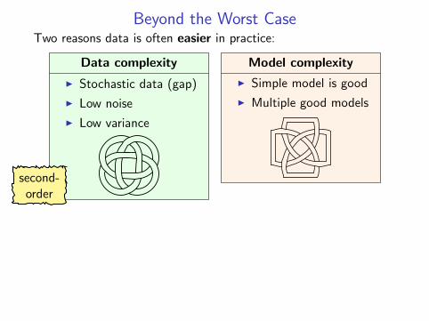
Beyond the Worst CaseTwo reasons data is often easier in practice:
Data complexity
I Stochastic data (gap)
I Low noise
I Low variance
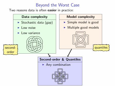
second-order
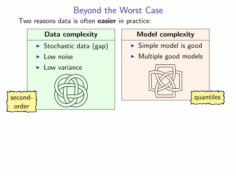
Model complexity
I Simple model is good
I Multiple good models
quantiles
Second-order & Quantiles
I Any combination
Beyond the Worst CaseTwo reasons data is often easier in practice:
Data complexity
I Stochastic data (gap)
I Low noise
I Low variance
second-order
Model complexity
I Simple model is good
I Multiple good models
quantiles
Second-order & Quantiles
I Any combination
Beyond the Worst CaseTwo reasons data is often easier in practice:
Data complexity
I Stochastic data (gap)
I Low noise
I Low variance
second-order
Model complexity
I Simple model is good
I Multiple good models
quantiles
Second-order & Quantiles
I Any combination
Beyond the Worst CaseTwo reasons data is often easier in practice:
Data complexity
I Stochastic data (gap)
I Low noise
I Low variance
second-order
Model complexity
I Simple model is good
I Multiple good models
quantiles
Second-order & Quantiles
I Any combination
Beyond the Worst CaseTwo reasons data is often easier in practice:
Data complexity
I Stochastic data (gap)
I Low noise
I Low variance
second-order
Model complexity
I Simple model is good
I Multiple good models
quantiles
Second-order & Quantiles
I Any combination
Beyond the Worst CaseTwo reasons data is often easier in practice:
Data complexity
I Stochastic data (gap)
I Low noise
I Low variance
second-order
Model complexity
I Simple model is good
I Multiple good models
quantiles
Second-order & Quantiles
I Any combination
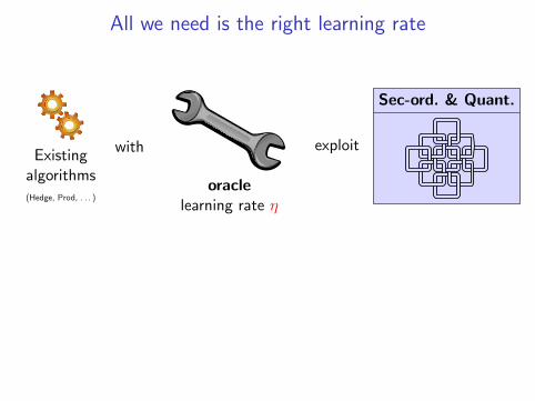
All we need is the right learning rate
Existingalgorithms(Hedge, Prod, . . . )
with
oraclelearning rate η
exploit
Sec-ord. & Quant.
Can we exploit Second-order & Quantiles on-line?

All we need is the right learning rate
Existingalgorithms(Hedge, Prod, . . . )
with
oraclelearning rate η
exploit
Sec-ord. & Quant.
Can we exploit Second-order & Quantiles on-line?
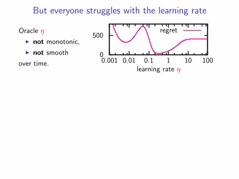
But everyone struggles with the learning rate
0
500
0.001 0.01 0.1 1 10 100learning rate η
regretOracle η
I not monotonic,
I not smooth
over time.
State of the art:
Second-order
Cesa-Bianchi, Mansour, and Stoltz 2007, Hazanand Kale 2010, Chiang, Yang, Lee, Mahdavi,Lu, Jin, and Zhu 2012, De Rooij, Van Erven,Grunwald, and Koolen 2014, Gaillard, Stoltz, andVan Erven 2014, Steinhardt and Liang 2014
or
Quantiles
Hutter and Poland 2005, Chaud-huri, Freund, and Hsu 2009, Cher-nov and Vovk 2010, Luo andSchapire 2014
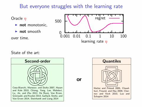
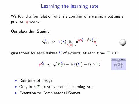
Learning the learning rate
We found a formulation of the algorithm where simply putting aprior on η works.
Our algorithm Squint
wkt+1 ∝ π(k) E
γ(η)
[eηR
kt−η2V k
t η]
Sec-ord. & Quant.
guarantees for each subset K of experts, at each time T ≥ 0:
RKT ≺√
VKT (− lnπ(K) + ln lnT )
I Run-time of Hedge
I Only ln lnT extra over oracle learning rate.
I Extension to Combinatorial Games
Overview
I Fundamental online learning problem
I Review previous guarantees
I New Squint algorithm with improved guarantees
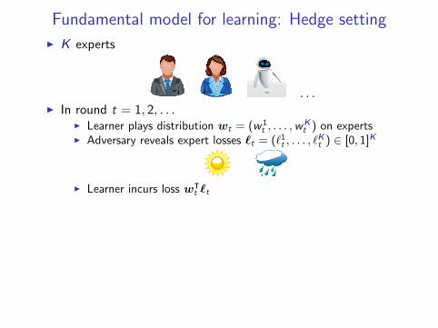
Fundamental model for learning: Hedge setting
I K experts
. . .
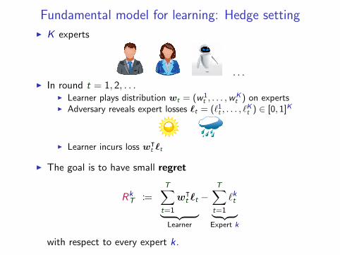
I In round t = 1, 2, . . .I Learner plays distribution wt = (w1
t , . . . ,wKt ) on experts
I Adversary reveals expert losses `t = (`1t , . . . , `Kt ) ∈ [0, 1]K
I Learner incurs loss wᵀt `t
I The goal is to have small regret
RkT :=
T∑t=1
wᵀt `t︸ ︷︷ ︸
Learner
−T∑t=1
`kt︸ ︷︷ ︸Expert k
with respect to every expert k .
Fundamental model for learning: Hedge setting
I K experts
. . .I In round t = 1, 2, . . .
I Learner plays distribution wt = (w1t , . . . ,w
Kt ) on experts
I Adversary reveals expert losses `t = (`1t , . . . , `Kt ) ∈ [0, 1]K
I Learner incurs loss wᵀt `t
I The goal is to have small regret
RkT :=
T∑t=1
wᵀt `t︸ ︷︷ ︸
Learner
−T∑t=1
`kt︸ ︷︷ ︸Expert k
with respect to every expert k .
Classic Hedge Result
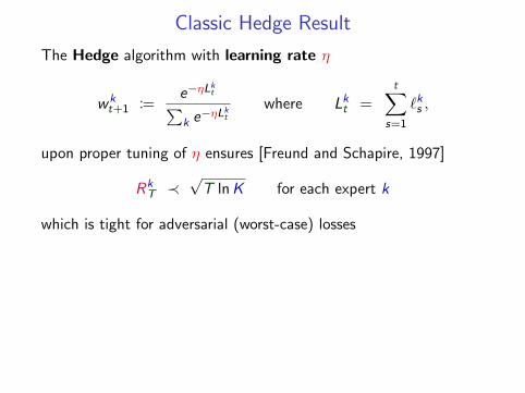
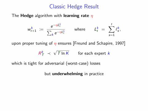
The Hedge algorithm with learning rate η
wkt+1 :=
e−ηLkt∑
k e−ηLkt
where Lkt =t∑
s=1
`ks ,
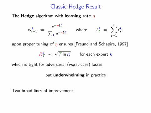
upon proper tuning of η ensures [Freund and Schapire, 1997]
RkT ≺
√T lnK for each expert k
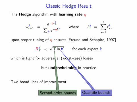
which is tight for adversarial (worst-case) losses
but underwhelming in practice
Two broad lines of improvement.
Second-order bounds Quantile bounds
Classic Hedge Result
The Hedge algorithm with learning rate η
wkt+1 :=
e−ηLkt∑
k e−ηLkt
where Lkt =t∑
s=1
`ks ,
upon proper tuning of η ensures [Freund and Schapire, 1997]
RkT ≺
√T lnK for each expert k
which is tight for adversarial (worst-case) losses
but underwhelming in practice
Two broad lines of improvement.
Second-order bounds Quantile bounds
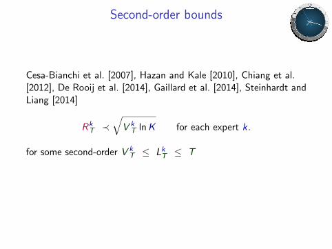
Second-order bounds
Cesa-Bianchi et al. [2007], Hazan and Kale [2010], Chiang et al.[2012], De Rooij et al. [2014], Gaillard et al. [2014], Steinhardt andLiang [2014]
RkT ≺
√V k
T lnK for each expert k.
for some second-order V kT ≤ LkT ≤ T
I Pro: stochastic case, learning sub-algorithms
I Con: specialized algorithms. hard-coded lnK .
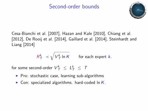
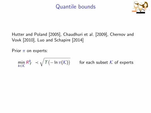
Quantile bounds
Hutter and Poland [2005], Chaudhuri et al. [2009], Chernov andVovk [2010], Luo and Schapire [2014]
Prior π on experts:
mink∈K
RkT ≺
√T(− lnπ(K)
)for each subset K of experts
I Pro: over-discretized models, company baseline
I Con: specialized algorithms. Efficiency. Inescapable T .
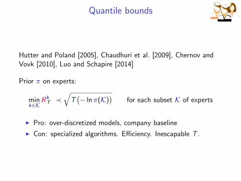
Quantile bounds
Hutter and Poland [2005], Chaudhuri et al. [2009], Chernov andVovk [2010], Luo and Schapire [2014]
Prior π on experts:
mink∈K
RkT ≺
√T(− lnπ(K)
)for each subset K of experts
I Pro: over-discretized models, company baseline
I Con: specialized algorithms. Efficiency. Inescapable T .
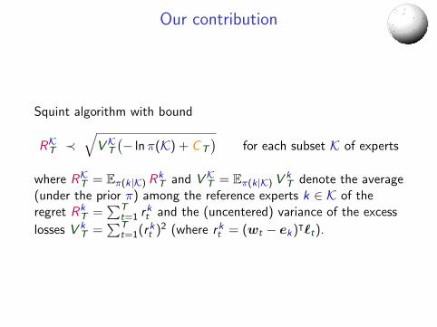
Our contribution
Squint algorithm with bound
RKT ≺√
VKT(− lnπ(K) + CT
)for each subset K of experts
where RKT = Eπ(k|K) RkT and VKT = Eπ(k|K) V k
T denote the average(under the prior π) among the reference experts k ∈ K of theregret Rk
T =∑T
t=1 rkt and the (uncentered) variance of the excess
losses V kT =
∑Tt=1(rkt )2 (where rkt = (wt − ek)ᵀ`t).
The cool . . .
I We aggregate over all learning rates
I While staying as efficient as Hedge
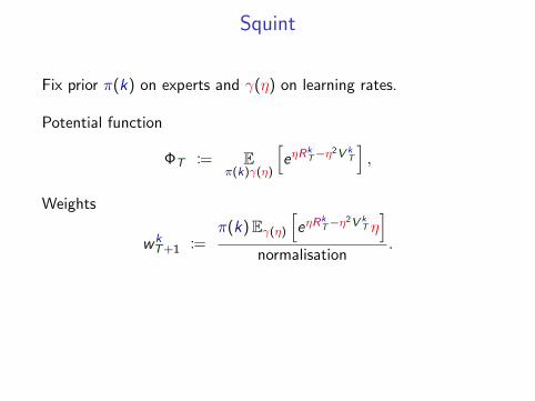
Squint
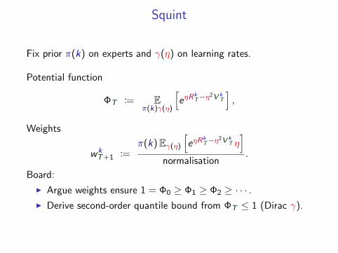
Fix prior π(k) on experts and γ(η) on learning rates.
Potential function
ΦT := Eπ(k)γ(η)
[eηR
kT−η2V
kT
],
Weights
wkT+1 :=
π(k)Eγ(η)[eηR
kT−η2V
kT η]
normalisation.
Board:
I Argue weights ensure 1 = Φ0 ≥ Φ1 ≥ Φ2 ≥ · · · .I Derive second-order quantile bound from ΦT ≤ 1 (Dirac γ).
Squint
Fix prior π(k) on experts and γ(η) on learning rates.
Potential function
ΦT := Eπ(k)γ(η)
[eηR
kT−η2V
kT
],
Weights
wkT+1 :=
π(k)Eγ(η)[eηR
kT−η2V
kT η]
normalisation.
Board:
I Argue weights ensure 1 = Φ0 ≥ Φ1 ≥ Φ2 ≥ · · · .I Derive second-order quantile bound from ΦT ≤ 1 (Dirac γ).
Squint
Fix prior π(k) on experts and γ(η) on learning rates.
Potential function
ΦT := Eπ(k)γ(η)
[eηR
kT−η2V
kT
],
Weights
wkT+1 :=
π(k)Eγ(η)[eηR
kT−η2V
kT η]
normalisation.
Board:
I Argue weights ensure 1 = Φ0 ≥ Φ1 ≥ Φ2 ≥ · · · .I Derive second-order quantile bound from ΦT ≤ 1 (Dirac γ).
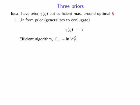
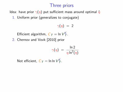
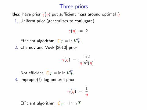
Three priors
Idea: have prior γ(η) put sufficient mass around optimal η
1. Uniform prior (generalizes to conjugate)
γ(η) = 2
Efficient algorithm, CT = lnVKT .
2. Chernov and Vovk [2010] prior
γ(η) =ln 2
η ln2(η)
Not efficient, CT = ln lnVKT .
3. Improper(!) log-uniform prior
γ(η) =1
η
Efficient algorithm, CT = ln lnT
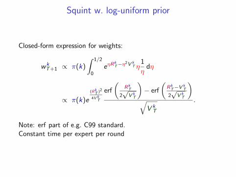
Squint w. log-uniform prior
Closed-form expression for weights:
wkT+1 ∝ π(k)
∫ 1/2
0eηR
kT−η2V
kT η
1
ηdη
∝ π(k)e
(RkT )2
4VkT
erf
(Rk
T
2√
V kT
)− erf
(Rk
T−VkT
2√
V kT
)√V k
T
.
Note: erf part of e.g. C99 standard.Constant time per expert per round
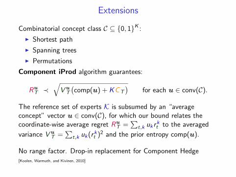
Extensions
Combinatorial concept class C ⊆ {0, 1}K :
I Shortest path
I Spanning trees
I Permutations
Component iProd algorithm guarantees:
RuT ≺
√V u
T
(comp(u) + KCT
)for each u ∈ conv(C).
The reference set of experts K is subsumed by an “averageconcept” vector u ∈ conv(C), for which our bound relates thecoordinate-wise average regret Ru
T =∑
t,k uk rkt to the averaged
variance V uT =
∑t,k uk(rkt )2 and the prior entropy comp(u).
No range factor. Drop-in replacement for Component Hedge[Koolen, Warmuth, and Kivinen, 2010]
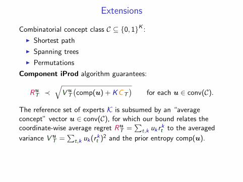
Conclusion
A fresh algorithm for an old problem.
I different
I efficient
I better

Thank you!