food security in portugal socioeconomic determinants … · this work uses household data to...
TRANSCRIPT
1
A Work Project, presented as part of the requirements for the Award of a Master’s
Degree in Economics from the NOVA – School of Business and Economics
FOOD SECURITY IN PORTUGAL – SOCIOECONOMIC
DETERMINANTS AND THE IMPACT OF THE PRODUCTION FOR
OWN-CONSUMPTION
José Ricardo Gonçalves Carrilho Sequeira
729
A project carried on the Master’s in Economics Program under the supervision of:
Professor Susana Peralta
Lisbon, May 22th, 2016
2
Food Security in Portugal – Socioeconomic Determinants and the
Impact of the Production for Own-Consumption
José Ricardo Sequeira1
Abstract
This work uses household data to analyse the determinants of food insecurity in Portugal, between
2004 and 2012, as well as the causal relationship between the production of goods for own-
consumption and food security. It is shown that own-production has a positive impact on food
security. Moreover, the financial crisis of 2008 did not negatively affect food security. The result
is robust to several specifications.
Keywords: Food Security; Own-Consumption; Instrumental Variables; Propensity Score
Matching
1. Introduction
In 1948, the Universal Declaration of Human Rights of the United Nations recognised the right to
food as part of the “right to an adequate standard of living”.2 In 1966, the International Covenant
on Economic, Social and Cultural Rights reiterated the “fundamental right of everyone to be free
from hunger” (Article11.2). More recently, in 2009, the FAO’s Declaration of the World Summit
1 I would like to express my heartfelt appreciation and gratitude for all the help and guidance provided by Professor
Susana Peralta, without whom this work would not have have been possible. Also, all the friends, family and
Professors with whom I shared moments and ideas that contributed to this thesis. 2 Article 25 of the Universal Declaration of Human Rights, 1948

3
on Food Security identified the four pillars of food security as availability, access, utilization and
stability.
The seminal work of Sen that won him a Nobel Prize in 1998, has changed the public and academic
discourse of the analysis of food in/security.3 Maxwell (1996), Hadley and Crooks (2012) and
Borch (2016) also show that the academic discourse of food security has shifted from being
production oriented (supply) to more household and consumption oriented (demand). As Sen
(1982) shows, there is a misconception that hunger is primarily the result of a deficit in global food
production, when in most cases of widespread famine-related deaths since World War II, food was
available in the area affected by the famine. Patel (2012) argues further that the problem of hunger
has to do with political and social configurations that surround power over food, rather than just
the mere existance or not of food near a hungry individual. Webb et al. (2006) also claims that
emphasizing food availability may lead to an over-reliance on agricultural solutions to problems
that actually have other origins. Following this line of thought, the UN issued a report in 2013,
claiming that one should take into account systemic considerations, and alerts for the need to a
structural change in the food production system, due to the challenges of the 21st century,4
consisiting in a “rapid and significant shift from conventional, monoculture-based and high-
external-input-dependent industrial production towards mosaics of sustainable, regenerative
production systems that also considerably improve the productivity of small-scale local farmers.”5
3 Borch, A. “Food security and food insecurity in Europe”, page 3 4 Population increase, especially in the most resource-constrained areas of the planet; environmental crisis; low
access to land and water. This is, as explained by the UN report, bound to increase the social and political tensions
around the world, as well as the linked migratory movements of starving and poor populations and international
conflicts over resources. 5 United Nations Conference on Trade and Development, “Trade and Environment Review 2013: Wake Up Before It
Is Too Late, Make Agriculture Truly Sustainable Now for Food Security in a Changing Climate”
4
Food insecurity also strikes the most vulnerable households in rich countries (4.7% in Portugal and
10.31% in Europe).6 Coleman-Jensen et al. (2014) study indicates that up to 14% of the population
in the USA have experienced food insecurity. Despite this, little knowledge has been produced on
this subject, according to Borch (2016), who further explains that the limited research that has been
produced tends to focus on the production of food rather than on people’s access to food.
This paper focuses on food security in Portugal, using household-level data that allows for the
analyses of the relationship between several household and individual characterisitics and the
individuals’ food security status in Portugal, from 2004 to 2012. This period emcompasses the
2008 financial crisis, thus allowing for an exploratory analysis on the food security status of the
population. On top of that, estimates of the impact of the production for own-consumption on food
security will also be studied, to assess the hypothesized positive impact of the decentralization of
food production in food security. Galhena et al. (2013) reviewed the literature on the economic,
social and environmental contributions of home gardens to communities in different socio-
economic contexts, and recognized the positive impacts of home gardens on food security and
malnutrition, even though most of the studies reviewed were on developing countries. However,
the need for more research and empirical data on the role of home gardens and their impact on food
security is stressed by the authors.
6 Percentages computed using the Eurostat EU-SILC database, from 2004 to 2012. According to Elanco, “Enough:
Dimensions of food security in Europe 2015” (based on data from the EU-SILC of 2013, except for Ireland, which
only has data for 2012), there are around 22.2 million households that experience food insecurity, which is around
10.5% of European households
5
2. Literature Review
2.1. Food insecurity in Developed Countries
Most of the existing literature focuses on food insecurity on developing countries7 that often leads
to malnutrition and serious health complications, ultimately leading to death. There are, however,
a few papers that focus on developed countries.
Caillavet et al. (2011) focused on food security amongst French adults, and concluded that food
security is higher in middle-aged individuals, if the individual has higher levels of education and
income, if the individual owns a house, or if the individual is currently a smoker. Méjean et al.
(2005), also in France, found that the debt of a household is negatively correlated with the status
of food security of the individuals living in it.
There are also a few papers dealing with the Portuguese case directly. Álvares (2013) using data
from the National Health Survey wave 2005/06, concludes that 17% of the population was food
insecure, and 3.7% were in a state of severe food insecurity. The factors associated with the
presence of food insecurity were being a female, being younger, having a lower education level,
having smoking habits and a lower self-evaluated health status. Also in Portugal, The General
Directorate for Health (DGS) of the Portuguese Government (2013) reports that 32.1%, 8.1% and
8.8% were respectively mildly, moderately and severely food insecure.8 The likelihood of being
food insecure inscreases with living in Algarve, being illiterate, being over 65 years of age or living
in a household with people over 65, being unemployed or a stay-at-home worker and poor health.
Conversely, secondary or post-secondary education and if the individual is living in a household
with 3 or 4 people increases food security.
7 State of Food Security in the World 2015, FAO 8 Direcção Geral de Saúde, Ministério da Saúde do Governo de Portugal, “Portugal: Alimentação Saudável em
números – 2013”

6
2.2. Food Insecurity in Developing Countries
The concern over food insecurity in developing countries has fostered a vast literature that focuses
on various individual and household level variables. Welderufael (2014) studied food insecurity in
Ethiopia, and concluded that it is more pervasive in rural areas. In urban areas, its main
determinants are large family sizes, with lower consumption expenditures, old age, unemployment
and being a male. Harris-Fry et al. (2015) established that wealth and literacy are associated with
improved food security, as well as the dietary diversity in women living in rural Bangladesh. Other
variables found to impact food security in developing countries were off-farm and non-farm
incomes, land and livestock holdings, soil and water conservation techniques, farm size and
distance to the market, quality of extension workers, gender, educational level and type of
household farm enterprise (Beyene et al. (2010) for Ethiopia, Kassie et al. (2012) for Kenya,
Amaza, P. S. (2006) for Nigeria).
2.3. Food Insecurity and Own-Consumption
Production of goods for own-consumption has been studied in economics, under the field of
Family/Household Economics9 and later on the New Home Economics.10 Also its impact on several
socio-economic outcomes has been studied. Frick et al. (2009) found that an increase in household
production led to a decrease in inequality across Germany.
Marsh (1998) showed that home gardens provide easy everyday access to a variety of fresh foods
for the owners who, correspondingly, obtained more than 50% of the vegetables and fruits from
their garden. Other studies concluded that, while adding to the caloric intake, home gardens
9 See for exemple Reid, M. (1934) “Economics of Household Production” 10 See for exemple Becker, G. S. (1981) “A Treatisie on the Family”
7
supplement a basic diet with a meaningful amount of proteins,11 minerals,12 and vitamins,13 leading
to an enriched and balanced diet.14 Considering a more urban setting, Cuba had a critical stage of
food insecurity, due to the loss of trade caused by the collapse of the socialist bloc, in 1989, as most
of its food and productive system depended on imports. As explained by Altieri et al. (1999), urban
agriculture, the so-called greening of the “barrios”, became a significant source of fresh produce
for the urban and suburban populations.15
What is more, the production of goods for own-consumption in home or community gardens is also
a propeller for the development of the local economies, as explained by Galhena et al. (2013), Jones
(2012), and the report by the not-for-profit organization Gardening Matters, “Multiple Benefits of
Community Garden” (2012), for example. A movement that promotes this type of decentralized
production is the Transition Movement that sprouted in the UK, and spreaded all over the world,
and includes the use of urban and peri-urban small-scale food production.16
3. Econometric approach
3.1. Methodology
A Linear Probability Model (LPM) was chosen to analyse food security, which allows a
straightforward interpretation of the covariates coefficients (Wooldridge, 2009).
11 Torquebiau E: Are tropical agroforestry gardens sustainable? Agric Ecosyst Environ 1992, 41:189–207 12 Asfaw Z, Woldu Z: Crop associations of home gardens in Welayta and Gurage in southern Ethiopia. Ethiopian J
Sci 1997, 20:73–90 13 Kumar BM, Nair PKR: The enigma of tropical homegardens. Agrofor Syst 2004, 61:35–152. 14 Pulami RP, Poudel D: Home Garden’s Contribution to Livelihoods of Nepalese Farmers. Pokhara, Nepal: Paper
presented at Home Gardens in Nepal: Proceeding of a workshop on Enhancing the contribution of home garden to
on-farm management of plant genetic resources and to improve the livelihoods of Nepalese farmers: Lessons learned
and policy implications (2004); 2006 15 During 1996, Havana’s urban farms provided the city’s urban population with 8,500 tons of agricultural produce, 4
million dozens of flowers, 7.5 million eggs, and 3,650 tons of meat. 16 To know more about the movement: https://www.transitionnetwork.org/ and Hopkins, R. (2008) “The Transition
Handbook”, Green Books
8
The inconvenience of the LPM is that it fails to take into account the truncation of the dependent
variables. However, the LPM works well for values of the independent variables that are near the
sample averages. On top of that, this is more of a problem if the aim of the model is to make
predictions, which is not the main objective of this paper. Hence, as long as the value of the
coefficients is not larger than 1 in absolute terms, the LPM can be used for analysing this type of
data (Wooldridge, 2009).
Finally, the linear probability model violates the Gauss-Markov assumption of homoskedasticity.
Following Guan (2003), bootstrapped standard errors that correct for heteroscedasticity were used
throughout the paper to allow for inference.
3.2.Data
The data used in this work are from the European Union Statistics on Living and Income Conditions
(EU-SILC), an annual EU-wide survey, ran aince 2004 by the Eurostat, with the aim of collecting
data on the structural indicators of social cohesion. SILC has become the EU reference source for
comparative statistics on income distribution and social exclusion at the European level. This work
used the panel microdata of the EU-SILC.
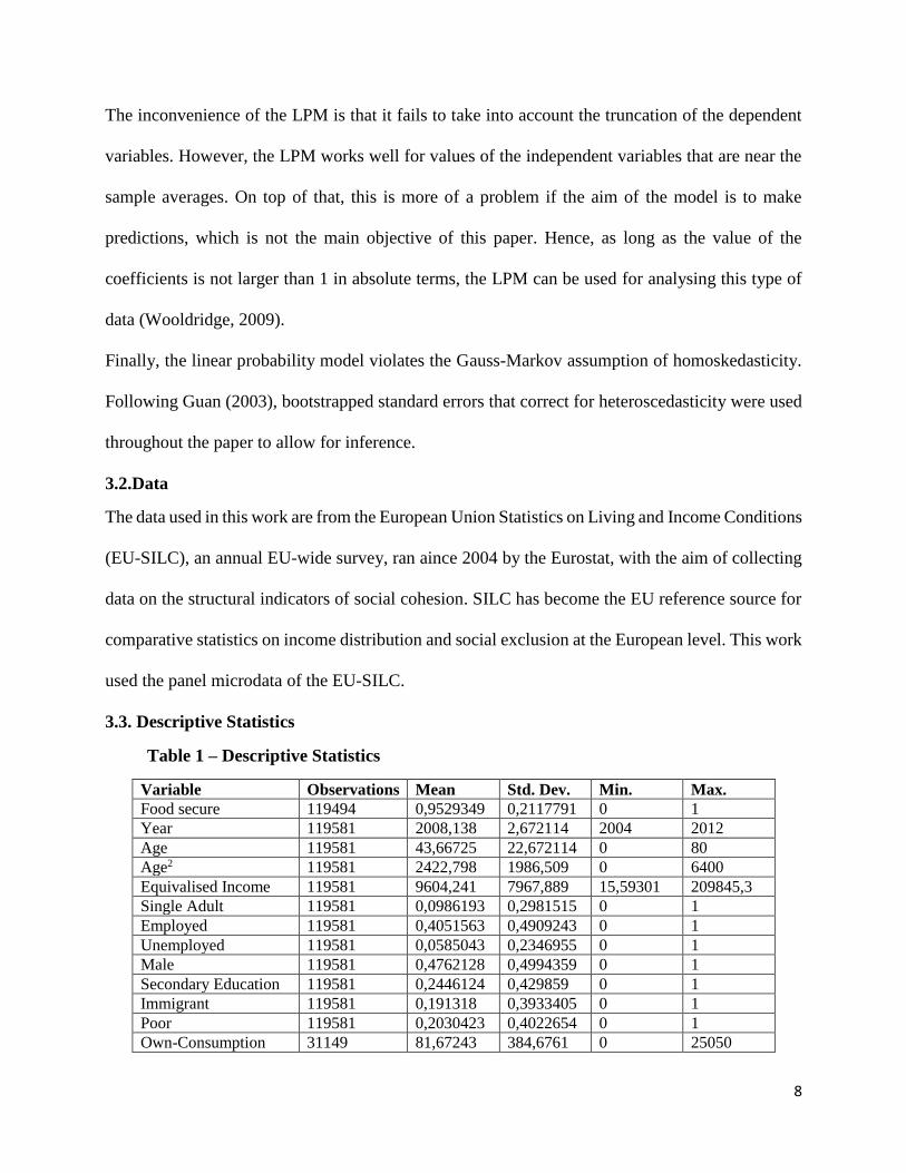
3.3. Descriptive Statistics
Table 1 – Descriptive Statistics
Variable Observations Mean Std. Dev. Min. Max.
Food secure 119494 0,9529349 0,2117791 0 1
Year 119581 2008,138 2,672114 2004 2012
Age 119581 43,66725 22,672114 0 80
Age2 119581 2422,798 1986,509 0 6400
Equivalised Income 119581 9604,241 7967,889 15,59301 209845,3
Single Adult 119581 0,0986193 0,2981515 0 1
Employed 119581 0,4051563 0,4909243 0 1
Unemployed 119581 0,0585043 0,2346955 0 1
Male 119581 0,4762128 0,4994359 0 1
Secondary Education 119581 0,2446124 0,429859 0 1
Immigrant 119581 0,191318 0,3933405 0 1
Poor 119581 0,2030423 0,4022654 0 1
Own-Consumption 31149 81,67243 384,6761 0 25050
9
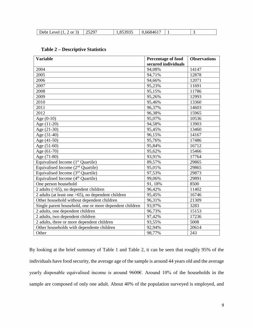
Debt Level (1, 2 or 3) 25297 1,853935 0,6684617 1 3
Table 2 – Descriptive Statistics
Variable Percentage of food
secured individuals
Observations
2004 94,08% 14147
2005 94,71% 12878
2006 94,66% 12071
2007 95,23% 11691
2008 95,15% 11786
2009 95,26% 12993
2010 95,46% 13360
2011 96,37% 14603
2012 96,38% 15965
Age (0-10) 95,07% 10536
Age (11-20) 94,58% 13903
Age (21-30) 95,45% 13460
Age (31-40) 96,15% 14167
Age (41-50) 95,76% 17486
Age (51-60) 95,84% 16712
Age (61-70) 95,62% 15466
Age (71-80) 93,91% 17764
Equivalised Income (1st Quartile) 89,57% 29865
Equivalised Income (2nd Quartile) 95,01% 29865
Equivalised Income (3rd Quartile) 97,53% 29873
Equivalised Income (4th Quartile) 99,06% 29891
One person household 91, 18% 8500
2 adults (<65), no dependent children 96,42% 11402
2 adults (at least one >65), no dependent children 95,45% 16746
Other household without dependent children 96,31% 21309
Single parent household, one or more dependent children 93,97% 3283
2 adults, one dependent children 96,73% 15153
2 adults, two dependent children 97,42% 17236
2 adults, three or more dependent children 93,55% 5008
Other households with dependente children 92,94% 20614
Other 98,77% 243
By looking at the brief summary of Table 1 and Table 2, it can be seen that roughly 95% of the
individuals have food security, the average age of the sample is around 44 years old and the average
yearly disposable equivalised income is around 9600€. Around 10% of the households in the
sample are composed of only one adult. About 40% of the population surveyed is employed, and
10
about 6% is unemployed. Also, about 25% of the population has secondary schooling and about
20% are immigrants.
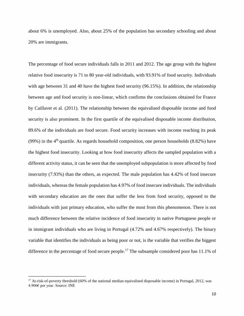
The percentage of food secure individuals falls in 2011 and 2012. The age group with the highest
relative food insecurity is 71 to 80 year-old individuals, with 93.91% of food security. Individuals
with age between 31 and 40 have the highest food security (96.15%). In addition, the relationship
between age and food security is non-linear, which confirms the conclusions obtained for France
by Caillavet et al. (2011). The relationship between the equivalised disposable income and food
security is also prominent. In the first quartile of the equivalised disposable income distribution,
89.6% of the individuals are food secure. Food security increases with income reaching its peak
(99%) in the 4th quartile. As regards household composition, one person households (8.82%) have
the highest food insecurity. Looking at how food insecurity affects the sampled population with a
different activity status, it can be seen that the unemployed subpopulation is more affected by food
insecurity (7.93%) than the others, as expected. The male population has 4.42% of food insecure
individuals, whereas the female population has 4.97% of food insecure individuals. The individuals
with secondary education are the ones that suffer the less from food security, opposed to the
individuals with just primary education, who suffer the most from this phenomenon. There is not
much difference between the relative incidence of food insecurity in native Portuguese people or
in immigrant individuals who are living in Portugal (4.72% and 4.67% respectively). The binary
variable that identifies the individuals as being poor or not, is the variable that verifies the biggest
difference in the percentage of food secure people.17 The subsample considered poor has 11.1% of
17 At-risk-of-poverty threshold (60% of the national median equivalised disposable income) in Portugal, 2012, was
4.906€ per year. Source: INE

11
food insecure individuals among them, whereas the not-poor subsample has only 3.08% of food
insecure individuals.
3.4. The determinants of household food insecurity in Portugal18
To assess food security, there was only one question that was constant in all the years that the
survey was performed19 – the capacity to afford a meal with meat, chicken, fish (or vegetarian
equivalent) every second day (HS050). This is an indicator of extreme food insecurity.
Table 1 shows the explanatory variables. Age has been shown to be an important determinant
(Caillavet et al., 2011). Since this relationship may not be linear, age squared is also introduced in
the regression. To further control for socio-economic characteristics of the individual, the
equivalised disposable income is included in the regression.20 To control for the composition of the
household, rather than just the number of people living in it, a dummy variable is included that
indicates if there is only one adult in the household. This includes families with single parents,
which are expected to have lower food security in developed countries,21 and also households
composed of just one person, assumed to be an adult. Included in the regression is also a dummy
variable that takes the value 1 if the individual is at work (employed) and 0 if it is not. The same
was done for unemployment. One’s status regarding the labor market is one of the most important
factors of deprivation.22 The reference group are the people out of the labor force (retired,
18 The identification code of the variables in the SILC database is presented in parenthesis (ex: food security status –
HS050) 19 There was a specific module on food security in the 2009 wave of SILC, with a few more questions regarding
eating habits. 20 The equivalised disposable income is the total income of a household, after tax and other deductions, divided by
the number of household members converted into equalised adults, i.e. each member of the household is equalised by
weighting each according to their age, using the OECD-modified scale. It is the scale currently used by Eurostat,
where the first adult is attributed a weight of 1.0, the second and each subsequent person aged 14 and over is
attributed a weight of 0.5, and a weight of 0.3 is attributed to each child aged under 14). This variable also to tries to
capture scale economies within the household (intrahousehold public goods). 21 USDA, Economic Research Service calculations using data from the December 2014 Current Population Survey
Food Security Supplement 22 Eurostat, Social Inclusion Statistics, 2016

12
youngsters and other inactive individuals). The regression also contains a dummy variable
controlling for biological gender (taking the value 1 if male, and 0 if female) and for education
(taking the value 1 if the individual attended secondary education, and 0 otherwise).
Following the analysis performed by Caillavet et al. (2011) in France and the report by the DGS
(2013) in Portugal, a dummy variable identifying the individual as an immigrant or not is also
included.23 The last variable included in the benchmark regression is a dummy identifying the
household as poor (HX080). This variable takes the value 1 if the household’s equivalised
disposable income is below 60% of the median of the equivalised disposable income for the whole
sampled population, and takes the value 1 otherwise. The “debt level” variable was not included in
the benchmark regression presented in the previous section, because it only has 25.297
observations, whereas all the other variables included in the benchmark regression have 119.581
observations. Year fixed effects are included in all the specifications, to account for the
macroeconomic context. The standard errors of the benchmark regression are bootstrapped.
4. Results
4.2. Regression Results
The regression controls for the yearly fixed effects. The results of the coefficients for each year are
presented in Graphic 1. The reference year is 2004. The possibility of food security being
negatively affected by the 2008 financial crisis and the years that followed is discarded by these
results.24
23 Both studies found this variable to be not significant. 24 All the regressions done in this work control for yearly fixed effects. However, we will not be focusing on the
coefficients from the year dummies, as that is not the mais focus of this work.

13
Graphic 1 – Yearly Fixed Effects of the LPM25
The results of the LPM are in column (1), Table 3. Age has a positive impact in the probability of
an individual being food secure. This means that as people get older, the probability of being food
secure increases. The variable age squared is found to be not statistically significant, suggesting a
linear relationship.
Socio-economic conditions all have the expected impacts: positive for the equivalised income,
being employed, having a secondary education, and being an immigrant;26 and negative for one
adult households, being unemployed and being poor. Being male does not impact the probability
of being food secure in a statistically significant way.
A goodness-of-fit measure that can be applied to this regression is the percent correctly predicted
observations. The regression estimated was able to correctly predict the outcome of 95.22% of the
observations.27
25 The value for 2006 is not statistically significant, for 2005 and 2008 are only statistically significant at 5%. The
coefficients for the remaining years are statistically significant at 1%. 26 This result contrast the previous literature, that had found this covariate to be not statistically significant. 27 A new variable was generated, that took the value 1 if the predicted value from the benchmark regression was equal
or bigger than 0,5 and took the value 0 otherwise. Then the percentage of the observations that took the value 1 for
both the food security status of the individual and the new variable generated was computed – this percentage
corresponds to the percentage of observations that were correctly predicted by the regression. This percentage is only
used for the evaluation of the goodness-of-fit of the regression.
0,00%
0,50%
1,00%
1,50%
2,00%
2,50%
Year 2005 Year 2006 Year 2007 Year 2008 Year 2009 Year 2010 Year 2011 Year 2012

14
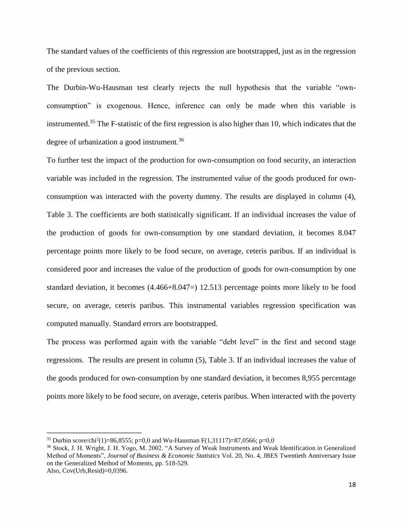
Table 3 – Regressions Results
Notes: bootstrapped standard errors are in parenthesis. * means stat. sig. at 10%, ** means stat. sig. at 5%, *** means
stat. sig. at 1%.
The Durbin-Wu-Hausman test was only performed on the first time the “own-consumption” was instrumented, to test
its endogeneity. Once the endogeneity was confirmed, the variable “own-consumption” should be (and is) instrumented
for every following regression.
Regional fixed effects: the only variable regarding this was DB040, which registered information on NUTS 1 and
NUTS 2. However, this variable was not defined for the Portuguese observations, so there is no possibility to include
it in the regression.
Software used: Stata.
5. Does production for own-consumption reduce food insecurity?
Food insecurity is a problem that affects the poorest individuals in the society, as it was just
documented by the previous results. The individual can have access to resources from several
Food Security LPM
(1)
LPM
(2)
IV
(3)
IV
(4)
IV
(5)
IV – Food
Security
Index
(6)
Probit – IV
(Margins)
(7)
Cons. 0,9165836 0,8839433 0,9114393 0,9421878 0,9446208 0,9431622
Age 0,0004036** (0,0001818)
0,0022506*** (0,0004797)
0,0012671*** (0,000477)
-0,000398** (0,0001756)
-0,0005812* (0,0003426)
-0,0019848 (0,0016925)
0,0134689*** (0,004935)
Age2 -1,41e-06
(2,09e-06)
-0,0000189***
(4,96e-06)
-0,0000161***
(4,77e-06)
5,48e-07
(1,96e-06)
2,17e-06
(3,92e-06)
6,81e-06
(0,0000186)
-0,000171***
(0,0000498)
Equivalised
Income
1,43e-06*** (4,42e-08)
1,20e-06*** (1,12e-07)
1,81e-06*** (1,83e-07)
1,92e-06*** (7,32e-08)
9,69e-07*** (1,40e-07)
3,47e-06*** (3,37e-07)
0,0000523*** (5,70e-06)
Single Adult -0,0247862***
(0,0024298)
-0,0270207***
(0,0053455)
-0,0209397***
(0,0047012)
-0,0189614***
(0,0024533)
0,0008822
(0,0050682)
0,0505945***
(0,0150986)
-0,1384464***
(0,0463237)
Employed 0,0131356*** (0,0017325)
0,0091024*** (0,0028888)
-0,0027558 (0,0038357)
0,0028032 (0,0013356)
0,001579 (0,0035102)
0,0072338 (0,108069)
-0,0424251 (0,039634)
Unemployed -0,0198088***
(0,003908)
-0,0223548***
(0,0058938)
-0,0213456***
(0,0062004)
-0,0189614***
(0,0035622)
-0,0154071**
(0,0061421)
0,0243834*
(0,013822)
-0,14142***
(0,0502648)
Male 0,0010315 (0,0011662)
0,0032257 (0,0023483)
-0,0298292*** (0,0048351)
-0,0265172*** (0,0020019)
-0,0176212*** (0,0034863)
-0,120464*** (0,0138887)
-0,3151912*** (0,551021)
Secondary
Education
0,0222031***
(0,0013706)
0,243934***
(0,0026183)
0,350566***
(0,0036228)
0,0310319***
(0,0013356)
0,014926***
(0,0029216)
0,0927697***
(0,007668)
0,4018318***
(0,0438801)
Immigrant 0,0209726*** (0,002616)
0,0119524** (0,004671)
0,0222457*** (0,0069118)
0,0294654*** (0,0027413)
0,0111636*** (0,0039578)
0,0503607*** (0,0109025)
0,2702521*** (0,0922839)
Poor -0,0618105***
(0,0020921)
-0,0593684***
(0,004819)
-0,065757***
(0,0038441)
-0,0800727***
(0,0029646)
-0,0400704***
(0,0061928)
-0,875519***
(0,015604)
-0,3432311***
(0,044752)
Own-
Consumption
-6,69e-07 (3,403-06)
0,0002843*** (0,0000338)
0,0002092*** (0,0000148)
0,0002328*** (0,0000391)
0,00088*** (0,0000956)
0,0030493*** (0,0004531)
Poor*Own-
Consumption
0,0000242***
(9,37e-06)
0,0001187***
(0,0000187)
0,0000174
(0,000067)
0,0001509*
(0,000088)
Debt Level 2 0,040584*** (0,0026846)
Debt Level 3 0,0407321***
(0,0026846)
Yearly Fixed
Effects
Y Y Y Y Y N Y
Number of
observations
119494 31132 31132 119494 25261 3065 31132
Adjusted R2 0,0320 0,0284 ----------------- 0,0344 0,0287 0,0880 ----------------
Wald chi2 (18) 5052,35 (14) 924,65 (13) 798,73 (20) 5421,08 (22) 832,20 (12) 219,25 (13) 621,23
Durbin Score
(IV)
86,8555
Wu-Hausman
(IV)
87,0566
Period of
analysis
2004-2012 2004-2012 2004-2012 2004-2012 2004-2012 2009 2004-2012
15
Government safety nets available, which have been proven to increase the food security of
individuals (Schmidt et al. (2012); Yen et al. (2008); Mykerezi (2010)).
At the individual level, the production of goods for own-consumption can be a way to increase the
income of individuals. This is especially interesting as most own-production concerns food -
subsistence agriculture has long been the major part of non-market household production.28 SILC
asks respondents to estimate the value of goods produced for own consumption (PY070N). This
was selected to be the variable of interest.29 This variable basically captures the value of the goods
for own consumption produced in the household garden, as explained by Atkinson (2010).30
This variable is introduced in the regression by itself, and interacted with the “poor” dummy, to see
if the poorest part of the society, which is also the most affected by this phenomenon, can increase
its probability of being food secure through the production for own-consumption. The results of
that regression are in column (2), Table 3. The variable is not statistically significant by itself, but
it is when interacted with the poverty dummy. If production for own-consumption increases by one
standard deviation31 per year, the individual becomes 0.93 percentage points more likely to be food
secure.
However, the coefficient of the variable by itself has a negative sign. This may be due to an
endogeneity bias, as own-production may result from a decision to avoid food insecurity amongst
the households who face that risk. The endogeneity problem was tackled with two different
approaches: Instrumental Variables and Propensity Score Matching.
28 “Measuring the Non-Observed Economy: A Handbook”, OECD, 2002 29 This variable refers to the market value of food and beverages produced and also consumed within the same
household in net terms, which is equal to the gross value with the respective tax deductions and social security
contributions, when applicable. 30 Atkinson, M. (2010) “Income and Living Conditions in Europe”, page 189 31 St. Dev.=384.6761
16
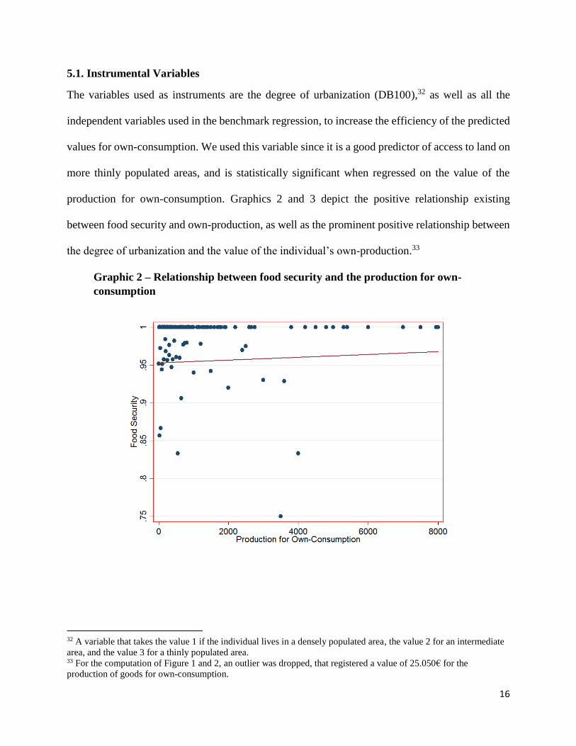
5.1. Instrumental Variables
The variables used as instruments are the degree of urbanization (DB100),32 as well as all the
independent variables used in the benchmark regression, to increase the efficiency of the predicted
values for own-consumption. We used this variable since it is a good predictor of access to land on
more thinly populated areas, and is statistically significant when regressed on the value of the
production for own-consumption. Graphics 2 and 3 depict the positive relationship existing
between food security and own-production, as well as the prominent positive relationship between
the degree of urbanization and the value of the individual’s own-production.33
Graphic 2 – Relationship between food security and the production for own-
consumption
32 A variable that takes the value 1 if the individual lives in a densely populated area, the value 2 for an intermediate
area, and the value 3 for a thinly populated area. 33 For the computation of Figure 1 and 2, an outlier was dropped, that registered a value of 25.050€ for the
production of goods for own-consumption.

17
Graphic 3 – Relationship between the degree of urbanization and the value of the
production for own-consumption
Imbens, Angrist and Rubin (1996) have shown that the coefficient of the instrumented variable can
be interpreted as a local average treatment effect specific to the instrument used. In this case, the
coefficient estimates the average of the effect of the production for own-consumption on the food
security status of the individuals whose production of goods for own-consumption has been
affected by the degree of urbanization.
As it can be seen in column (3), Table 3, when instrumented, the variable “own-consumption” is
statistically significant. If an individual increases the value of the production of goods for own-
consumption by one standard deviation, it becomes 10.93 percentage points more likely to be food
secure, on average, ceteris paribus.34
34 An instrumental variables approach was taken as well, but with a probit model for robustness purposes. The result
of the marginal interpretation is consistent with the findings of the LPM IV results, and are presented in column (7),
Table 3. If an individual increases the value of the production of goods for own-consumption by one standard
deviation, it becomes 117.3 percentage points more likely to be food secure, on average, ceteris paribus. The result is
the same if the marginal result is at means.
18
The standard values of the coefficients of this regression are bootstrapped, just as in the regression
of the previous section.
The Durbin-Wu-Hausman test clearly rejects the null hypothesis that the variable “own-
consumption” is exogenous. Hence, inference can only be made when this variable is
instrumented.35 The F-statistic of the first regression is also higher than 10, which indicates that the
degree of urbanization a good instrument.36
To further test the impact of the production for own-consumption on food security, an interaction
variable was included in the regression. The instrumented value of the goods produced for own-
consumption was interacted with the poverty dummy. The results are displayed in column (4),
Table 3. The coefficients are both statistically significant. If an individual increases the value of
the production of goods for own-consumption by one standard deviation, it becomes 8.047
percentage points more likely to be food secure, on average, ceteris paribus. If an individual is
considered poor and increases the value of the production of goods for own-consumption by one
standard deviation, it becomes (4.466+8.047=) 12.513 percentage points more likely to be food
secure, on average, ceteris paribus. This instrumental variables regression specification was
computed manually. Standard errors are bootstrapped.
The process was performed again with the variable “debt level” in the first and second stage
regressions. The results are present in column (5), Table 3. If an individual increases the value of
the goods produced for own-consumption by one standard deviation, it becomes 8,955 percentage
points more likely to be food secure, on average, ceteris paribus. When interacted with the poverty
35 Durbin score/chi2(1)=86,8555; p=0,0 and Wu-Hausman F(1,31117)=87,0566; p=0,0 36 Stock, J. H. Wright, J. H. Yogo, M. 2002. “A Survey of Weak Instruments and Weak Identification in Generalized
Method of Moments”, Journal of Business & Economic Statistics Vol. 20, No. 4, JBES Twentieth Anniversary Issue
on the Generalized Method of Moments, pp. 518-529.
Also, Cov(Urb,Resid)=0,0396.

19
indicator it is not statistically significant, evidencing that the effect is the same regardless if the
individual is poor or not.
5.2. Propensity Score Matching
Another regression technique that can be used to establish causality between variables is propensity
score matching (PSM), which is a useful approach when only observed characteristics such as
education, the locality of residence, family composition, degree of poverty, etc. are believed to
affect “program participation” 37, which in this case is having a home garden that produces food.
The ideal experiment would be to have two individuals with the same propensity to have a garden
with the same size of own-production of goods, but actually only one of them having it. This way
it can be assumed that differences in the propensity to be food secure of these two individuals is
solely attributed to fact that one produces good for its own-consumption and the other does not.
Usually this framework of analyses is implemented when the treatment variable is binary, i.e.
having a home garden or not. However, this information is not readily available in the SILC, which
only reports the value of the goods produced for own-consumption, which is a continuous variable
that takes values between 0 and 8000.38 To perform the PSM analyses, this variable was divided
by quintiles, conditional on it taking a strictly positive value. Each quintile has 793 observations,39
and the maximum values for each quintile are, respectively, 100, 260, 500, 1000 and 8000.
Then, several dummy variables were created that identified the observations as being part of each
quintile, or having a production of 0.40 This way, a PSM analyses could be performed for each of
37 Khandker, et al. “Handbook on Impact Evaluation: Quantitative Methods and Practices”, 2010, The World Bank 38 One outlier was dropped, that presented a value of 25.050€. 39 On average. Due to the fact that there are some values that verify a very high number of observations, some
quintiles have more observations than others (Q1=803; Q2=784; Q3=1015; Q4=770; Q5=593). 40 Observations that reported a missing value when answering the question regarding the value of the goods produced
for own-consumption were not considered.

20
treatment level.41 This methodology allows for the construction of the following graph (Graphic
4), which comprises information on the average treatment on the treated (ATT) for each quintile
of production as well as the respective significance level. The propensity scores were computed
with a 5% significance level, the matching was obtained through nearest neighbor matching with
replacement, following the theoretical reasoning of Rubin (1973) and the practical application of
Becker and Ichino (2002), and satisfy the balancing property.42
Graphic 4 – ATT of Producing Goods for Own-Consumption on Food Security43
The results show that, when compared with an individual with no production, individuals in the 1st,
2nd, and 3rd quintile of the distribution are 1.2, 2.8, and 2.9 percentage points more likely to be able
to afford the reference meal, respectively. The estimate for the ATT for the values in the 4th and 5th
quintiles is not statistically significant.
The same procedure was performed again, but this time including the variable “debt level”. The
following graph (Graphic 5) was constructed, already with the balancing property satisfied in every
case:
41 The degree of urbanization was included in the regression. 42 Several covariates had to be dropped to satisfy the balancing condition. Procedure done following “Handbook on
Impact Evaluation: Quantitative Methods and Practices”, page 181. 43 Dark grey: statistically significant at 1%; Light grey: statistically significant at 10%; White: not statistically
significant
0,00%
0,50%
1,00%
1,50%
2,00%
2,50%
3,00%
3,50%
1st Quintile 2nd Quintile 3rd Quintile 4th Quintile 5th Quintile
21
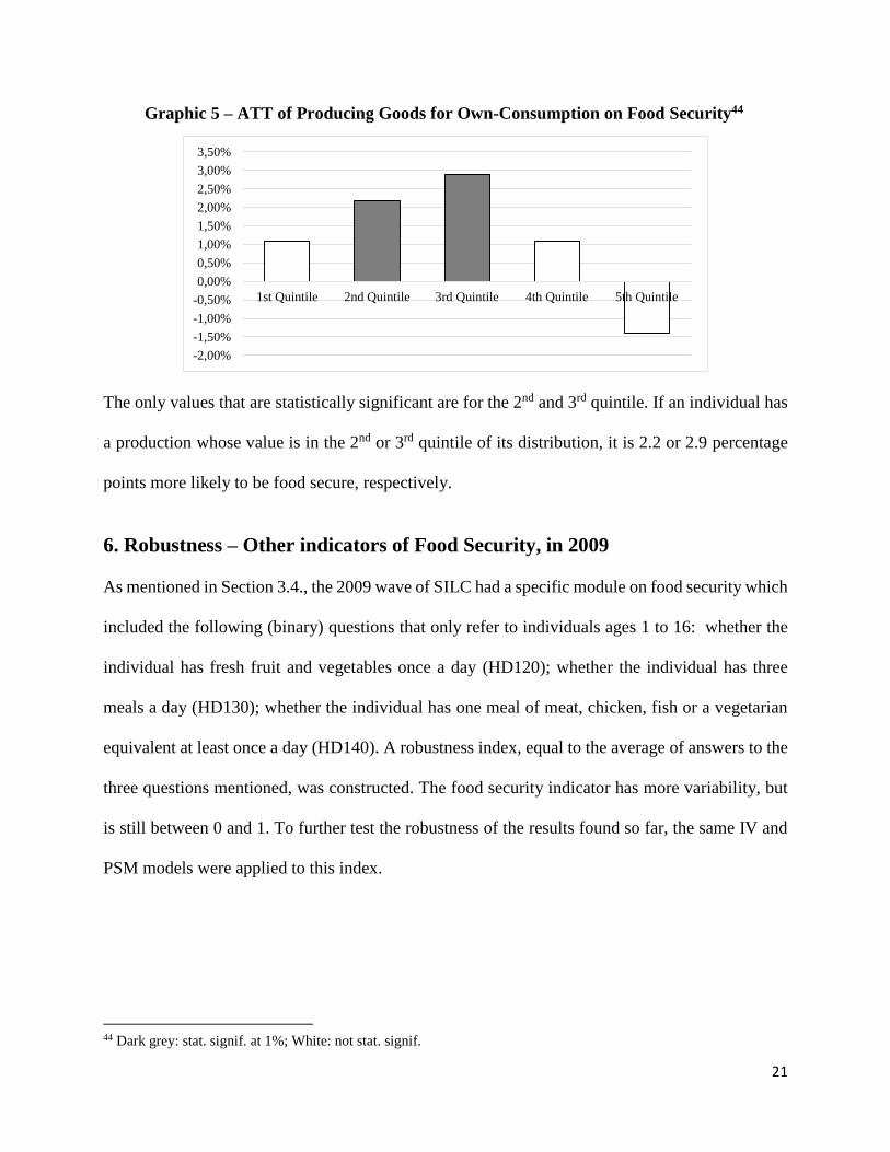
Graphic 5 – ATT of Producing Goods for Own-Consumption on Food Security44
The only values that are statistically significant are for the 2nd and 3rd quintile. If an individual has
a production whose value is in the 2nd or 3rd quintile of its distribution, it is 2.2 or 2.9 percentage
points more likely to be food secure, respectively.
6. Robustness – Other indicators of Food Security, in 2009
As mentioned in Section 3.4., the 2009 wave of SILC had a specific module on food security which
included the following (binary) questions that only refer to individuals ages 1 to 16: whether the
individual has fresh fruit and vegetables once a day (HD120); whether the individual has three
meals a day (HD130); whether the individual has one meal of meat, chicken, fish or a vegetarian
equivalent at least once a day (HD140). A robustness index, equal to the average of answers to the
three questions mentioned, was constructed. The food security indicator has more variability, but
is still between 0 and 1. To further test the robustness of the results found so far, the same IV and
PSM models were applied to this index.
44 Dark grey: stat. signif. at 1%; White: not stat. signif.
-2,00%
-1,50%
-1,00%
-0,50%
0,00%
0,50%
1,00%
1,50%
2,00%
2,50%
3,00%
3,50%
1st Quintile 2nd Quintile 3rd Quintile 4th Quintile 5th Quintile

22
6.1. Instrumental Variables with Other Dependent Variables
Similar to what was done in section 5.1, the degree of urbanization is used to instrument the value
of own-consumption. The results are in column (6), Table 3, and they confirm the previous
conclusions. If an individual increases its production of goods for own-consumption in one
standard deviation, its probability of being food secure increases by 35.59 percentage points.45 If
an individual is considered poor and increases the value of the production of goods for own-
consumption by one standard deviation, it becomes (35.59+6.103=) 41.693 percentage points more
likely to be food secure, on average, ceteris paribus.
6.2. Propensity Score Matching with Other Dependent Variables
The PSM procedure was performed just the same as in section 5.2, but this time with the dependent
variable being the index constructed. The quintiles for the distribution of the value of the goods
produced for own-consumption were estimated again, just for the year 2009, and the maximum
values for the 1st, 2nd, 3rd, 4th, and 5th quintile are 150, 300, 500, 1000 and 7950, respectively. Each
quintile has 295 observations.46 The following graph (Graphic 6) was constructed with the results:
Graphic 6 – ATT of Producing Goods for Own-Consumption on Food Security47
45 St. Dev. of own-consumption is 404.4159 for the year 2009. 46 On average. Due to the fact that there are some values that verify a very high number of observations, some
quintiles have more observations than others (Q1=380; Q2=302; Q3=254; Q4=291; Q5=246). 47 Dark grey: stat. signif. at 1%; White: not stat. signif.
0,00%
1,00%
2,00%
3,00%
4,00%
5,00%
6,00%
1st Quintile 2nd Quintile 3rd Quintile 4th Quintile 5th Quintile
23
This analysis confirms the results previously found, regarding the causality established. If the
production of goods for own-consumption is in the first, second or third quintile of its distribution,
the probability of being food secure increases by 5.7, 5.0 and 5.4 percentage points, respectively.
The results for the 4th and 5th quintile are not statistically significant.
7. Conclusions, limitations and areas for further research
This paper studies the determinants of food insecurity in Portugal, between the years of 2004 and
2012. Most, but not all, of the determinants that impact food security were as hypothesized and as
expressed in the previous literature. Age, equivalised income, being employed, having more
education, being an immigrant,48 and producing goods for own-consumption have a positive impact
on food security. Being in a single adult household, being unemployed, being male,49 being poor
and having a higher burden of debt negatively impact food security. The production of goods for
own-consumption in home gardens is found to have a positive causal relationship with the food
security of the individual. Being poor increases this positive relationship. This result is robust to
several regression specifications, and indicates that the decentralized small-scale own-production
of food may be a source of income for individuals, and hence increasing their probability of having
food security.
However, the results of this paper have limitations. The first relates to the nature of the data. It
relies on self-reported data, in particular regarding the value of production for own consumption.
This is prone to measurement error (Atkinson and Marlier, 2010). Moreover, we fit a regression to
a rare event, which may overstate the value of the coefficients. However, this problem is somewhat
mitigated by the large number of observations in the sample used (Gao and Shen, 2007).
48 This result contrast the previous literature, that had found this covariate to be not statistically significant. 49 This result contrast the findings of Álvares (2013).
24
The second limitation relates to the PSM and IV approaches. If the decision to have a home garden
with production for own-consumption is not based on observable characteristics, the PSM results
will be biased. We were only able to use one IV, given the nature of the data. More instrumental
variables should be tested using other databases, to check whether the results of this paper carry on
to other settings. More importantly, there is the need to further testing the possibility that the degree
of urbanization may be endogenous to the production of goods for own-consumption.50
The third limitation refers to the type of food insecurity analyzed. EU-SILC only allows for
knowledge on individuals with severe food insecurity. More information regarding several levels
of food insecurity (mild, average, severe) should be inquired for future analysis. Steps in this
direction are being taken by the research project http://www.saudepontocome.pt/ that is collecting
a thorough database of eating habits in Portugal.
Finally, this work project points to the importance of home gardens in promoting food security. It
also motivates the need to further our knowledge on this topic. Whether there are effective ways to
promote these and the design of such programs is an area of future research. For instance, the
“hortas urbanas” project of the Lisbon municipality could have a built-in experimental design that
would allow the academic community to test its impact on food security and, more generally, on
healthy eating habits and also as a source of income for individuals.
50 However it can be assumed that this variable (degree of urbanization) is exogenous at least for the most vulnerable
individuals in society.
25
8. Bibliography
1. Altieri, M. Companioni, N. Cañizares, K. Murphy, C. Rosset, P. Bourque, M. Nicholls, C. 1999 “The greening of the
“barrios”: Urban agriculture for food security in Cuba.” Agriculture and Human Values 16: 131–140
2. Amaza, P.S., Umeh, J.C., Helsen, J. Adejobi A.O. 2006. “Determinants and measurement of food insecurity in Nigeria:
Some empirical policy guide.” Contributed paper prepared for presentation at the international association of
agricultural economics conference, Gold coast, Australia. 3-8
3. Angrist, J. D. Imbens, G. W. Rubin, D. B. 1996. “Identification of Causal Effects Using Instrumental Variables.”
Journal of the American Statistical Association Vol. 91, No. 434, pp. 444-455
4. Asfaw Z, Woldu Z. 1997. “Crop associations of home gardens in Welayta and Gurage in southern Ethiopia.” Ethiopian
J Sci, 20:73–90
5. Atkinson, M. Marlier, E. 2010. “Income and Living Conditions in Europe”, Luxembourg: Publications Office of the
European Union, page 189
6. Becker, G. S. 1981, Enlarged ed., 1991. “A Treatise on the Family”. Cambridge, MA: Harvard University Press. ISBN
0-674-90698-5
7. Becker, S. O. Ichino, A. 2002. “Estimation of average treatment effects based on propensity scores.” The Stata Journal
2, Number 4, pp. 358–377
8. Beyene, F. Muche, M. 2010. “Determinants of Food Security among Rural Households of Central Ethiopia: An
Empirical Analysis.” Quarterly Journal of International Agriculture 49, No. 4: 299-318
9. Borch A. 2016. “Food security and food insecurity in Europe: An analysis of the academic discourse (1975–2013).”
Appetite, doi: 10.1016/j.appet.2016.04.005
10. Caillavet, F. Touazi, D. Darmon, N. 2011. “Food insecurity, health restriction and poverty among French adults:
Implications for public policies.” EAAE Congress Change and Uncertainty
11. Coleman-Jensen, A. Rabbitt, M. P. Gregory, C. Singh, A. 2014. “Household food insecurity in the United States in
2014.” United States Department of Agriculture, Economic, Research Service Report no 194.
12. DGS. 2013. “Portugal: Alimentação Saudável em números – 2013” , Ministério da Saúde do Governo de Portugal
13. Elanco. 2015. “Enough: Dimensions of food security in Europe 2015”
14. FAO, IFAD and WFP. 2015. “The State of Food Insecurity in the World 2015 Meeting the 2015 international hunger
targets: taking stock of uneven progress.” Rome, FAO
15. Frick, J. R. Grabka, M. M. Groh-Samberg, O. 2009. “The impact of home production on economic inequality in
Germany.” IZA Discussion Papers, No. 4023, http://nbn-resolving.de/urn:nbn:de:101:1-20090304806
16. Galhena, D. H. Freed, R. Maredia, K. M. 2013. “Home gardens: a promising approach to enhance household food
security and wellbeing.” Agriculture & Food Security, 2-8 DOI: 10.1186/2048-7010-2-8
17. Gao, S. Shen, J. 2007: “Asymptotic properties of a double penalized maximum likelihood estimator in logistic
regression.” Statistics and Probability Letters 77: 925- 930.
18. Gardening Matters. 2012. “Multiple Benefits of Community Garden”, Online Publication:
http://www.gardeningmatters.org/

26
19. Guan, W. 2003. “From the help desk: Bootstrapped standard errors”, The Stata Journal, page 72-73
20. Hadley, D. Crooks, D. L. 2012. “Coping and the biosocial consequences of food insecurity in the 21st century”.
Yearbook of Physical Anthropology, 55, 72-94
21. Harris-Fry, H. Azad, K. Kuddus, A. Shaha, S. Nahar, B. Hossen, M. Younes, L. Costello, A. Fottrell, E. 2015. “Socio-
economic determinants of household food security and women’s dietary diversity in rural Bangladesh: a cross-sectional
study.” Journal of Health, Population and Nutrition 33:2 DOI 10.1186/s41043-015-0022-0
22. Hopkins, R. 2008. “The Transition Handbook: From oil dependency to local resilience”, Green Books
23. Jones, L. 2012 “Improving Health, Building Community: Exploring the Asset Building Potential of Community
Gardens.” Evans School Review, Vol. 2, Num. 1
24. Kassie, M. Ndiritu, S. W. Shiferaw, B. 2012. “Determinants of Food Security in Kenya, a Gender Perspective.” 86th
Annual Conference of the Agricultural Economics Society, University of Warwick, United Kingdom
25. Khandker, S. R. Koolwal, G. B. Samad, H. A. 2010. “Handbook on Impact Evaluation: Quantitative Methods and
Practices”, The World Bank, Washington, D. C.
26. Kumar, B. M. Nair, P. K. R. 2004. “The enigma of tropical homegardens.” Agrofor Syst, 61:35–152
27. Marsh, R. 1998. “Building on traditional gardening to improve household food security.” Food Nutr Agr, 22:4–14
28. Maxwell, S. 1996. “Food security: a post-modern perspective.” Food Policy, 21(2), 155–170
29. Méjean, C. Deschamps, V. Bellin-Lestienne, C. Oleko, A. Darmon, N. Hercberg, S. Castetbon, K. 2010. “Associations
of socioeconomic factors with inadequate dietary intake in food aid users in France”, European Journal of Clinical
Nutrition 64, 374–382
30. Mykerezi, E. 2010. “The Impact of Food Stamp Program Participation on Household Food Insecurity”, Amer. J. Agr.
Econ. 92(5): 1379–1391
31. OECD. 2002. “Measuring the Non-Observed Economy: A Handbook”, OECD Publications
32. Patel, R. C. 2012. “Food sovereignty: Power, gender, and the right to food”. PLoS Med 9(6): e1001223.
doi:10.1371/journal.pmed.1001223
33. Pulami, R. P. Poudel, D. 2004;2006 “Home Garden’s Contribution to Livelihoods of Nepalese Farmers.” Pokhara,
Nepal: Paper presented at Home Gardens in Nepal: Proceeding of a workshop on Enhancing the contribution of home
garden to on-farm management of plant genetic resources and to improve the livelihoods of Nepalese farmers: Lessons
learned and policy implications
34. Reid, M. G. 1934. “Economics of Household Production.” New York: J. Wiley & Sons
35. Rubin, D.B. 1973. “Matching to remove bias in observational studies.” Biometrics, 29:159–184
36. Schmidt, L. Shore-Sheppard, L. Watson, L. 2012. “The Effects of Safety Net Programs on Food Insecurity”. University
of Kentucky Center for Poverty Research Discussion Paper Series, DP2012-12
37. Sen, A. 1982. “Poverty and famines: An essay on entitlement and deprivation.” Oxford: Oxford University Press
38. Stock, J. H. Wright, J. H. Yogo, M. 2002. “A Survey of Weak Instruments and Weak Identification in Generalized
Method of Moments”, Journal of Business & Economic Statistics Vol. 20, No. 4, JBES Twentieth Anniversary Issue
on the Generalized Method of Moments, pp. 518-529
39. Torquebiau, E. 1992. “Are tropical agroforestry gardens sustainable?” Agric Ecosyst Environ, 41:189–207

27
40. UNCTAD. 2013. “Trade and Environment Review 2013: Wake Up Before It Is Too Late, Make Agriculture Truly
Sustainable Now for Food Security in a Changing Climate.” United Nations Publications, ISSN 1810-5432
41. Webb, P. Coates, J. Frongillo, E. A. Rogers, B. L. Swindale, A. Bilinsky, P. 2006. “Measuring household food
insecurity: why it's so important and yet so difficult to do.” J Nutr 136(5), 1404S–1408S.
42. Welderufael, M. 2014. “Determinants of Households Vulnerability to Food Insecurity in Ethiopia: Econometric
analysis of Rural and Urban Households”, Journal of Economics and Sustainable Development Vol.5, No.24,
www.iiste.org ISSN 2222-1700 (Paper) ISSN 2222-2855 (Online)
43. Wooldridge, J. M. 2009. “Introductory Econometrics: A Modern Approach.” South Western College Publications, 4th
ed.
44. Yen, S. T. Andrews, M. Chen, Z. Eastwood, D. 2008. “Food Program Participation and Food Insecurity: An
Instrumental Variables Approach”, Amer. J. Agr. Econ. 90(1): 117–132