food price crisis in indonesia: alert from the key...
TRANSCRIPT

Food Price Crisis in Indonesia: Alert from the Key Markets
Irfan Mujahid*a and Matthias Kalkuhl*b
*) Center for Development Research (ZEF), University of Bonn
Selected Paper prepared for presentation at the 2015 Agricultural & Applied
Economics Association and Western Agricultural Economics Association Annual
Meeting, San Francisco, CA, July 26-28
Copyright 2015 by [authors]. All rights reserved. Readers may make verbatim copies of
this document for non-commercial purposes by any means, provided that this copyright
notice appears on all such copies.

2
Food Price Crisis in Indonesia: Alert from the Key Markets
Irfan Mujahid1 and Matthias Kalkuhl
Center for Development Research (ZEF), University of Bonn.
Abstract
Food price variations can be very costly when they abrupt and unanticipated. In
the current new era of market uncertainty, monitoring food prices become
highly important to foresee any potential crisis. This study proposes an
alternative approach in monitoring food price movements in many different
markets within a country by focusing only on the key markets. Using monthly
retail rice prices from the 25 major markets in Indonesia, we identify the key
markets whose price movements can help to forecast price movements in all
other markets. The key markets are identified using granger causality tests
conducted in the vector error correction model framework. The relevance of
monitoring the key markets in detecting price crisis is tested using Probit and
Poisson models. We found that albeit not all of alert phases lead to crises,
monitoring the key markets can help to forecast price movements in all markets
across the country.
Keywords: volatility, crisis, transmission, early warning system, Indonesia.
JEL Classification: C22, F1, F47, Q1
1 Corresponding Author: [email protected]

3
Introduction
Indonesia is the largest economy in Southeast Asia and the fourth most populous country in
the world2 (UN DESA, 2013). The country consists of more than 13 thousand islands; with
around 6 thousand of them are inhabitants3. Notwithstanding the high economic growth in the
past decade, Indonesia is still home for 30 million people living under poverty line and an
additional 65 million people vulnerable to poverty (World Bank, 2012). These poor
households, who are like many others in the developing countries, spend more than half of their
income on food (von Braun and Tadesse, 2012). Thus, soaring food prices in the recent years
plays an important role in the purchasing power of a large part of Indonesian population,
bringing threats to their food and nutrition security.
Figure 1. Food price index of selected countries 2001 - 2014
Source: FAOSTAT
Furthermore, in the recent years, Indonesia experiences high food price volatility accompanied
by high risk of food and nutrition insecurity. Using food price index data from ILOSTAT and
combined anthropometric data from WHO, UNICEF and World Bank, Mujahid and Kalkuhl
(2014) show that Indonesia is among countries that experience “high” or “very high” food price
volatility as well as “high” or “very high” chronic and acute malnutrition. Moreover, evidences
have shown that the increase of food prices raises the rate of poverty in Indonesia (Ivanic et.
al., 2012; Warr and Yusuf, 2013).
2 After China, India and USA 3 Badan Informasi Geospasial/Geospatial Information Body http://www.bakosurtanal.go.id/ accessed December
5th, 2014.
1.4
1.6
1.8
2
2.2
2001 2002 2003 2004 2005 2006 2007 2008 2009 2010 2011 2012 2013 2014
Index
Year
China
Indonesia
India

4
In this context, monitoring food price movements becomes highly important for Indonesia
which can help to better anticipate any potential of “abnormal” food prices in the country.
Given the peculiar geographic characteristic of Indonesia, where markets are spread in its
archipelago, an efficient approach in monitoring food price movement is needed. Using the
concept of price transmission and market integration, we investigate whether price movements
in many different markets in the country can be monitored by focusing only on the key markets.
Furthermore, we analyze the relevance of monitoring the key markets in detecting potential
price crisis events in Indonesia.
The approach is based on the information provided by market price. Market is assumed to be
efficient which its prices reflect all available information not only on current food availability
but also on agents’ expectations about future scarcity (Deaton and Laroque, 1992; Ravallion,
1985). Similar to this approach, Araujo et al. (2012) use price signals to detect potential price
crises in Mali, Burkina Faso and Niger.
The rest of this paper is organized as follows: the next section provides context of the analysis
and description of price data that will be used. Section 3 explores the prices in the 25 markets
in Indonesia to further define price crisis. Section 4 aims to identify the key markets whose
prices can be used to forecast price movements in all other markets. In section 5, we test the
relevance of using the key markets to detect price crisis. Section 6 provides summary and
conclusion.
Context and data description
Food supply in Indonesia mostly comes from own production. Rice, sugar and palm oil are the
three largest quantities being produced in the country. Nevertheless, supplies of some food
commodities are not met by own production, including rice, Indonesians’ main staple food
which accounted for nearly half of their calorie’s intake. Indonesia is still importing around 3-
6 percent of their domestic rice supplies annually to fulfill high demand in the country
(FAOSTAT, 2014).

5
Figure 2. Indonesian’s per capita calorie intake 2011
Source: own elaboration based on FAOSTAT
For many years, price stabilization in Indonesia was managed by Badan Urusan Logistik
(BULOG), a national food reserve agency created in 1968 with a special objective to protect
domestic markets from sharp fluctuations of prices on world markets. The end of New Order
regime in late 1990s was the emerging era of more open trade policy in Indonesia. The country
loosened its monopoly structure and created competitions within the domestic market. BULOG
lost its domestic power to monopolize sugar and rice trade because Indonesia was required to
comply with the IMF Letter of Intent to make market more efficient. After finishing the
engagement with IMF, Indonesia decided to shift to a more managed trade policy and started
to impose tariffs on sugar and rice imports.
The policy was not long lasting as Indonesia started to create more liberal economy by reducing
tariffs. Since then, export oriented policies have been the picture of Indonesia’s agricultural
trade policy. Agricultural exports increased by 16 percent on average annually during 2004-
2009 (Octaviani et al., 2010). However, in this ‘Reform Era’ in which the market was relatively
open, food prices were relatively higher and more volatile than it was before, when BULOG
has a strong power to intervene the market (figure 3). Estimations of volatility using standard
deviations of log of prices in difference (SSD) for some commodities including rice, sugar,
wheat flour and cooking oil show that the SSD are much higher for the periods after 1998
compare to the periods before 1998. Nevertheless, BULOG ran at high fiscal cost. A financial
wheat6%
maize8%
cassava5%
sugar5%
palm oil4%
rice49%
fruits 3%
vegetables2%
others18%

6
audit report by Arthur Anderson covering the period of April 1993 to March 1998 suggested
that total inefficiency of BULOG was about 400 million USD per year (Arifin, 2008).
Figure 3. Prices of several food commodities in Indonesia before and after major reform
SSD before 1998=0.058 after 1998 = 0.105 SSD before 1998=0.036 after 1998 = 0.127
SSD before 1998=0.039 after 1998 = 0.106 SSD before 1998=0.030 after 1998 = 0.156
Note: SSD=Standard deviations of log of prices in difference
Source: Own estimations based on BPS/Statistics Indonesia data
Our focus in this study is rice, the main staple food for Indonesians. The analysis uses monthly
retail rice prices from 25 major markets in Indonesia for the periods of 2000 - 2013. The sample
markets in this study are among the 33 main markets of the capital city provinces in Indonesia
which spread in its 5 main islands and 30 other smaller islands. The data come from Badan
Pusat Statistik (BPS), a national bureau of statistics of Indonesia. BPS regularly publishes the
weighted average of several different types of rice that are sold in all major retail markets in
Indonesia.

7
Figure 4. Sample markets
Source: own elaboration.
Food Price Movement: Defining the Crisis
Despite a relatively well established concept of food security4, no common definition of food
price crisis can be found in the literature (Cuesta et al, 2014). In fact, without any clear concept,
the term food price crisis is widely known and used for analytical and operational purposes,
especially in the light of explaining the global excessive price volatility and spike events in
2008 and 2011.
At this point, it is important to understand the different terms that are commonly used to explain
price dynamics. von Braun and Tadesse (2012) observed that most studies on food price
dynamics focus on high food prices. They argue, however, that price movements should be
distinguished as trend, volatility and spike.
A price trend is the smooth, long-term average movement of prices over time that shows the
general tendency of prices for a certain period of time. Price volatility refers to frequent short-
term fluctuations of the prices around a rather stable long-term price or price trend. It measures
the strength and frequency of the price changes. In general, both positive and negative
variations affect price volatility. There are sets of methods available in the literature to analyze
price volatility, the common ways include: (i) coefficient of variation from mean or trend
4 FAO concept of food security “food security exists when all people, at all times, have physical and economic
access to sufficient, safe and nutritious food for a healthy and active life” is considered to be widely accepted.

8
(Huchet-Bourdon, 2011), (ii) changes of log returns (Gilbert and Morgan, 2010) and (iii)
GARCH model (Roache, 2010; Karali and Power, 2013).
Figure 5. Food price volatility in the global and Indonesia markets
Note: The global market (upper map) uses the monthly food price index for the period 2000 – 2012 taken from
ILO database. The Indonesia market (lower map) uses monthly retail rice price data for the period 2000 – 2013
taken from Statistics of Indonesia.
Source: Mujahid and Kalkuhl (2014) and own elaboration.
Figure 5 presents volatility map in the global and Indonesia food market, estimated using the
coefficient of variation from trend. The upper map shows the rate of food price volatility in
different countries which shows that Indonesia is among the high rates of volatility compare to
all other countries for the period 2000-2012. The lower map shows the rate of volatility in the
different markets in Indonesia for the period 2000-2013. It divides the markets into quintiles
and shows that Padang, Pekanbaru, Banjarmasin and Palangkaraya experience the highest

9
volatility among all major markets in Indonesia. Another term is price spike which is closely
related to price volatility. While volatility measures the price changes over a certain period,
price spike is usually measured as a relative change of prices over two consecutive periods.
The most common way to measure price spike is using percentage change as the logarithm of
the rate of period-over-period prices.
Not all price movements are troublesome. Price variations can be very costly only when they
abrupt and unanticipated by the economic agents (HLPE, 2011). It is also important to note
that price changes may have different impacts on the different economic agents. High food
prices can be incentives for net food producers to produce more food. More income can be
generated when food prices are on the upward trend relative to input prices. On the other hand,
high food prices negatively impact consumers. Poor people will have to spend much more of
their income on food when the prices are higher.
In the absence of a common definition of food price crisis, for the purpose of the analysis, this
study will limit the definition of the crisis to only from the customer point of view. According
to our definition, food price is considered as a crisis when the observed price is above a certain
level of the price that can be considered as normal. We first estimate the trend for each market
over the whole period using Hodrick-Prescott-filter (HP filter). The HP filter is widely used to
remove cyclical component of macroeconomic time series data to obtain a smoothed-curved
representation of the series which can be written as:
min𝜏
(∑(𝑦𝑡 − 𝜏𝑡)2
𝑇
𝑡=1
+ ∑[(𝜏𝑡+1 − 𝜏𝑡) − (𝜏𝑡 − 𝜏𝑡−1)]2
𝑇−1
𝑡=2
)
The first term of the equation is the sum of the squared deviations 𝑑𝑡 = 𝑦𝑡 − 𝜏𝑡 which
penalizes the cyclical component. The second term is a multiple smoothing parameter () of
the sum of squares of the trend component’s second differences. This second term penalizes
variation in the growth rate of the trend component. The larger the , the larger the penalty. As
recommended for monthly data, is chosen to be 129600.

10
Figure 6. Rice price and trend in Jakarta
Source: own elaboration
Our definition on “abnormal” price i.e. the price above certain level of price that can be
considered as normal, comes from relative spread not the absolute one because of price
inflations and long-term trends increase the absolute spread in both directions (positive and
negative). For instance, an increase of Rp.100/kg is large if the price is Rp.200/kg but small
if the price is Rp.1000/kg. To obtain relative spread, we divide the price series by its HP-price
trend which is normalized to 1 where we can observe only relative fluctuation. We further
estimate the standard deviation from these relative fluctuations for the analyzed period. We
consider price is in crisis when the relative spread between the relative price and its mean value
is greater than two standard deviation (figure 6).
200
04
00
06
00
08
00
01
00
00
120
00
rupia
h/k
g
2000m1 2005m1 2010m1 2015m1monthly
rice price Jakarta trend

11
Figure 7. Food price crisis in Jakarta
Source: own elaboration
Key Markets Identification
The approach in monitoring food price movements by focusing only on the key market
proposed in this study uses the concept of spatial price transmission and market integration.
The key theoretical concept in spatial price transmission analysis is spatial arbitrage, which
implies that the difference between prices of homogeneous goods in different markets is only
subject to transaction costs. Therefore, most of empirical works in spatial price transmission
analysis aim at assessing whether the Law of One Price holds true or not (Listorti and Esposti,
2012).
Our analysis aims to measure the degree of integration in each market and uses the information
to analyze how markets are being connected each other. Two markets are defined as being
integrated when shocks arising in one market are transmitted to the other market (Fackler and
Goodwin, 2001). More specifically, market i for good x is said to be spatially integrated with
market j for the same good if a shock in i that changes, for instance, demand in i but not in j,
.8.9
11
.11
.21
.3
price
/tre
nd
2000m1 2005m1 2010m1 2015m1monthly
relative rice price Jakarta critical value = mean + 2 sd

12
affects the prices in both i and j. This implies that the price series for homogenous commodity
in the two markets shared a long run stochastic trend.
We perform granger causality tests that are conducted in the vector error correction (VEC)
model framework to identify the key markets whose prices can help to forecast price
movements in other markets. The granger causality is a statistical hypothesis test which
suggests whether one time series is useful in forecasting another (Granger, 1969). In this study,
we test whether there is a causal relationship between current prices on market i and lagged
prices on market j.
The VEC model is appropriate to analyze short term and long term effects of one price on
another when two conditions are met. First, every price series is non stationary and integrated
to degree 1, which can be written as (I(1)), and second, the two or more series are co-integrated.
When two I(1) are co-integrated, there is a linear combination of the two series that is
stationary. In this study, we are analyzing two prices at a time, so that the co-integrating
equation can be written as:
𝑃𝑖 = 𝛼 + 𝛽𝑃𝑗 + 휀 or 휀 = 𝑃𝑖 − 𝛼 − 𝛽𝑃𝑗, where 휀 is stationary.
We test the stationary of each price series using Augmented Dickey Fuller (ADF) and the
results show that the price series for each market is stationary at (I(1))5. Each pair of the series
is also found to be co-integrated, which means that there is a long run relationship between
prices of two markets. We estimate the VEC model for each pair of the price series using the
following formulation:
∆𝑃𝑡𝑖 = 𝛼 + 𝜃(𝑃𝑡−1
𝑖 − 𝛽𝑃𝑡−1𝑗
) + 𝛿∆𝑃𝑡−1𝑗
+ 𝜌∆𝑃𝑡−1𝑗
+ 휀𝑡
Where 𝑃𝑡𝑖 is the price of market i and 𝑃𝑡
𝑗 is the price of market j. ∆ is the difference operator,
so ∆𝑃𝑡 = 𝑃𝑡 − 𝑃𝑡−1. 𝛼, 𝜃, 𝛽, 𝛿, 𝜌 are the estimated parameters and 휀 is error term.
By having already concluding that each pairs of the price series are co-integrated, meaning that
the two series have a long-run causal relationship, the causality being tested in the VEC model
indicate a short-run granger causality. It is important to note that if i is said to be granger causes
j, does not imply that j is the result of i. Granger causality measures precedence and information
content, but does not by itself indicate causality in the more common term. Here, the Granger
5 ADF test results can be found in appendix.
13
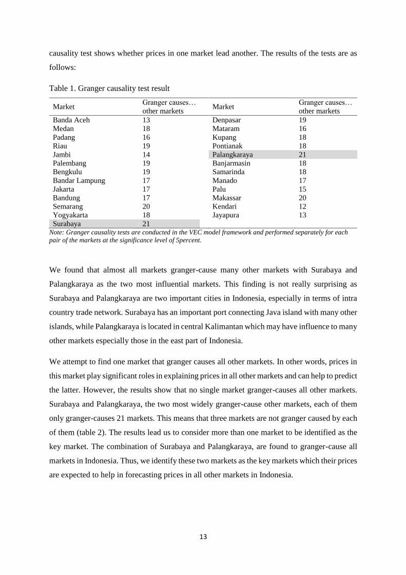
causality test shows whether prices in one market lead another. The results of the tests are as
follows:
Table 1. Granger causality test result
Market Granger causes…
other markets Market
Granger causes…
other markets
Banda Aceh 13 Denpasar 19
Medan 18 Mataram 16
Padang 16 Kupang 18
Riau 19 Pontianak 18
Jambi 14 Palangkaraya 21
Palembang 19 Banjarmasin 18
Bengkulu 19 Samarinda 18
Bandar Lampung 17 Manado 17
Jakarta 17 Palu 15
Bandung 17 Makassar 20
Semarang 20 Kendari 12
Yogyakarta 18 Jayapura 13
Surabaya 21 Note: Granger causality tests are conducted in the VEC model framework and performed separately for each
pair of the markets at the significance level of 5percent.
We found that almost all markets granger-cause many other markets with Surabaya and
Palangkaraya as the two most influential markets. This finding is not really surprising as
Surabaya and Palangkaraya are two important cities in Indonesia, especially in terms of intra
country trade network. Surabaya has an important port connecting Java island with many other
islands, while Palangkaraya is located in central Kalimantan which may have influence to many
other markets especially those in the east part of Indonesia.
We attempt to find one market that granger causes all other markets. In other words, prices in
this market play significant roles in explaining prices in all other markets and can help to predict
the latter. However, the results show that no single market granger-causes all other markets.
Surabaya and Palangkaraya, the two most widely granger-cause other markets, each of them
only granger-causes 21 markets. This means that three markets are not granger caused by each
of them (table 2). The results lead us to consider more than one market to be identified as the
key market. The combination of Surabaya and Palangkaraya, are found to granger-cause all
markets in Indonesia. Thus, we identify these two markets as the key markets which their prices
are expected to help in forecasting prices in all other markets in Indonesia.

14
Table 2. Granger causality test for the key markets
Key Market Not granger causes..
Surabaya Jakarta, Banjarmasin, Makassar
Palangkaraya Pekanbaru, Samarinda, Palu
Detecting Price Crisis by Monitoring the Key Markets
This section is devoted to test the relevance of using the key markets to predict the price crisis
in the country. As defined previously, we consider price is in crisis when the relative spread
i.e. the spread between the relative price and its mean value is greater than two standard
deviation. We will first determine an alert indicator that expected to predict the crisis. Further,
the probability of the alert that leads to a crisis is tested econometrically using Probit and
Poisson regressions.
Alert Indicator
We first distinguish the periods of “abnormal” prices based on the relative spread of the prices.
The crisis phase, where the spread between the relative price and its mean value is more than
two standard deviation, is usually preceded by a phase of an increasing price that moves from
the level that can be considered as normal. We will consider the periods of this increasing price
as an alert phase. It is the periods when the spread of the relative price is more than one standard
deviation but below two standard deviation (figure 7). Our alert indicator to predict potential
crisis in any market in the country will be the alert phase of the two key markets. The following
Probit and Poisson models will test whether it is relevant to observe the alert indicator in the
key markets to predict crisis in other markets.

15
Figure 7. Alert and crisis phases in the key markets
Source: Own elaboration
Probit Model
Probit model, also called probit regression, is used to model dichotomous or binary outcome
variables. The inverse standard normal distribution of the probability is modeled as a linear
combination of the predictors. This test aims at testing the probability of the alert in the key
markets that leads to a crisis in any market of the country. The dependent variable is a binary
variable taking value 1 if one or more markets are in the crisis phase at time t and 0 otherwise.
The independent variable is a binary variable of the alert phase of each key market, taking
value of 1 if the key market is on alert and 0 otherwise. A regression model is created by
parameterizing the probability of the price crisis to depend on a regressor of the alert phase of
the key market where:
𝑝𝑖𝑡∗ = 𝛽𝑥𝑘𝑡 + 휀𝑖𝑡
𝑝𝑖𝑡∗ is the latent dependent variable which refers to the probability of the crisis; 𝑝𝑖𝑡 is the
observed binary outcome variable defined as:
𝑝𝑖𝑡 = {1 𝑖𝑓 𝑝𝑖𝑡
∗ > 0
0 𝑜𝑡ℎ𝑒𝑟𝑤𝑖𝑠𝑒
𝑥𝑘𝑡−1 is the alert phase at the lagged value of each key market and 휀𝑘𝑡 is error term. We test
the alert phase of Surabaya and Palangkaraya that may lead to crisis in any market of the
country separately.
.91
1.1
1.2
1.3
price
/tre
nd
2000m1 2005m1 2010m1 2015m1monthly
relative rice price Surabaya crisis line = mean + 2 sd
alert line = mean + 1 sd
.6.8
11
.21
.4
price
/tre
nd
2000m1 2005m1 2010m1 2015m1monthly
relative rice price Palangkaraya crisis line = mean + 2 sd
alert line = mean + 1 sd
crisis phase
alert phase
crisis phase
alert phase

16
The results of the tests are as follows:
Table 3. Probit regression result
Key Market Coefficient Marginal Effect
Surabaya 0.8334***
(0.2987) 0.21
Palangkaraya 1.0597***
(0.3682) 0.28
Note: Standard errors are in parentheses, * p<0.1, ** p<0.05, *** p<0.01
We found that the coefficients of the key markets for the tests are positive and significant with
0.83 for Surabaya and 1.06 for Palangkaraya. The marginal effect for Surabaya is 0.21 while
for Palangkaraya is 0.28. This means that when Surabaya is on alert, the probability of any
other market that will be in crisis in the following month increases by 0.21 and when
Palangkaraya is on alert, the probability of any other market will be in crisis in the following
month increases about 0.28 percent.
Poisson Model
Another test is performed by Poisson regression that seeks to explain the extent of the crisis.
The outcome is the number of markets within the country that will be in crisis if the key market
is on alert. The Poisson regression is found to be appropriate when the dependent variable is a
count data. In this test, the dependent variable is the number of market that is in crisis within
the country, while the independent variable remains the same as in Probit regression which is
a binary variable of the alert phase of each key market, taking value of 1 if the key market is
on alert and 0 otherwise.
The basic Poisson probability specification can be written as:
𝑓(𝑦𝑡|𝑥𝑡) = 𝑒𝜇𝜇𝑦𝑡
𝑦𝑡!
Where 𝑦𝑡 is factorial, it is the number of markets that is experiencing a price crisis at time t. 𝑥𝑡
is the alert phase of each key market and 𝜇 is the parameter of Poisson distribution. For 𝜇 > 0, the
mean and variance of this distribution can be shown to be:
𝐸(𝑦) = 𝑣𝑎𝑟(𝑦) = 𝜇

17
Since the mean is equal to the variance, any factor that affects one will also affects the other,
thus, the usual assumption of homoscedasticity would not be appropriate for Poisson data.
The results of the Poisson tests are as follows:
Table 4. Poisson regression result
Key Market Coefficient Marginal Effect
Surabaya 0.6806***
(0.2278) 0.44
Palangkaraya 1.6771***
(0.3480) 1.13
Note: Standard errors are in parentheses, * p<0.1, ** p<0.05, *** p<0.01
The coefficient for Surabaya and Palangkaraya both are found to be positive and significant
with 0.68 for Surabaya and 1.68 for Palangkaraya and the marginal effect for Surabaya is 0.44
while for Palangkaraya is 1.13. This means that an alert in Surabaya leads to an increase of the
number of other markets that will be in crisis by 0.44 and an alert in Palangkaraya leads to an
increase of the number of other markets that will be in crisis by 1.13.
Summary and Conclusion
Indonesia is found to be among the countries that experience high food price volatility
accompanied by high risk of food and nutrition security (Mujahid and Kalkuhl, 2014).
Maintaining food prices at a sustainable level is prime important for a developing country such
Indonesia, where the large part of its citizen spend more than half of their income on food.
Thus, uncertainty as a result of food price volatility brings threats to their food and nutrition
security. This study investigates price movements in the major markets in Indonesia, identifies
the key markets and analyzes whether price movements in all markets in the country can be
monitored by focusing only on the key markets.
Using monthly retail rice prices from 25 major markets in Indonesia for the periods of 2000-
2013, we identify the key markets using granger causality tests that are conducted in the VEC
model framework. The results show that Surabaya and Palangkaraya can be considered as the
key markets whose price movements can help to explain prices in all other markets. This
finding is not surprising as Surabaya and Palangkaraya are two important cities in the trade
network within Indonesia. Surabaya has an important port connecting Java island with many

18
other islands and Palangkaraya is located in central Kalimantan which may have influence to
many other markets especially those in the east part of Indonesia.
We also test econometrically the relevance of using the information from the key markets to
predict potential crisis in the country using Probit and Poisson models. The Probit regression
results show that when Surabaya is on alert, the probability of any other market that will be in
crisis increases by 0.83 and when Palangkaraya is on alert, the probability of any other market
will be in crisis increases about 1.06 percent. In the Poisson regressions, the results show that
an alert in Surabaya leads to an increase of the number of other markets that will be in crisis
by 0.68 and an alert in Palangkaraya leads to an increase of the number of other markets that
will be in crisis by 1.68 percent.
While the findings can be interpreted as not all alerts phases lead to a crisis, the positive and
significant results of the regressions show the relevance of monitoring the key markets to
forecast price movements in many other markets. When the key markets are on alerts, the
probability of the price to move to a crisis is higher than the probability
This study shows an efficient approach in monitoring price movement using the information
from the market price. In a large developing country such Indonesia, where markets are located
in different islands with considerable distances, the results become important as it is possible
to monitor price movement in the country with less resource. By monitoring only Surabaya and
Palangkaraya, price movement in the 25 markets in Indonesia can be forecasted. Although the
results indicate that not all alert phases lead to a crisis, monitoring price movement can help to
better anticipate possible price crisis events. While one may argue that the cost of monitoring
food prices in all markets is low in the current new era of information technology, the proposed
study can serve as an alternative approach which can be useful in integrating policies between
different markets.

19
References
Abbott, P. 2010. Stabilization Policies in Developing Countries after the 2007-2008 Crisis.
Global Forum on Agriculture Policies for Agricultural Development, Poverty Reduction and
Food Security, 29–30 November, OECD, Paris.
Abbott, P., C. Hurt, and E. Tyner. 2011. What’s Driving Food Prices in 2011? Oak Brook, IL,
USA: Farm Foundation, NFP.
Anderson, K., 2012. Government Trade Restrictions and International Price Volatility. Global
Food Security 1, 157–166.
Anderson, K. and S. Nelgen. 2012. Trade Barrier Volatility and Agricultural Price
Stabilization. World Development 40 (1): 36-48.
Anderson, K., S. Jha, S. Nelgen, and A. Strutt. 2012. Reexamining Policies for Food Security
in Asia. Working Paper Series No. 301. Asian Development Bank, Manila.
Araujo, C., C. Araujo-Bonjean And S. Brunelin. 2012. Alert at Maradi: Preventing Food
Crises by Using Price Signals. World Development Vol. 40, No. 9, Pp. 1882–1894.
Arezki, R. and M. Brückner. 2014. Effects of International Food Price Shocks on Political
Institutions in Low-Income Countries: Evidence from an International Food Net-Export Price
Index. World Development, 61, 142-153.
Arifin, B. 2008. From Remarkable Success Stories to Troubling Present: The Case of BULOG
in Indonesia in Rashid, S. Gulati, A. and Cummings Jr., R. From Parastatals to Private Trade:
Lessons from Asian Agriculture. IFPRI, Washington DC.
Basri, M. C. and A. A. Patunru. 2012. How to Keep Trade Policy Open: the Case of Indonesia.
Bulletin of Indonesian Economic Studies 48 (2): 191-208.
Block, S. A., L. Kiess, P. Webb, S. Kosen, R. Moench-Pfanner, M. W. Bloem, C. P. Timmer.
2004. Macro Shocks and Micro Outcomes: Child Nutrition during Indonesia’s Crisis.
Economics and Human Biology 2, 21–44.
BPS (Badan Pusat Statistik/Statistics Indonesia). 2012. Statistical yearbook of Indonesia 2012.
Jakarta.
Brahmbhatt, M. and L. Christiaensen. 2008. Rising Food Prices in East Asia: Challenges and
Policy Options. Washington DC: World Bank.
Cameron, C., and P. Trivedi, 1990. Regression Based Tests for Over Dispersion in the Poisson
Model. Journal of Econometrics 46(3): 347–364.

20
Cuesta, J., A. Htenas and S. Tiwari. 2014. Monitoring Global and National Food Price Crises.
Food Policy 49. Pp. 84 – 94.
Dawe, D. 2008. Can Indonesia Trust the World Rice Market?. Bulletin of Indonesian Economic
Studies. Vol. 44, No. 1, 115-132.
Dawe, D. and P. Timmer. 2012. Why Stable Food Prices are a Good Thing: Lessons from
Stabilizing Rice Prices in Asia. Global Food Security 1, 127–133.
Deaton, A., and G. Laroque. 1992. On the Behaviour of Commodity Prices. Review of
Economic Studies, 59, 1–23.
de Hoyos, R.E. and D. Medvedev. 2011. Poverty Effects of Higher Food Prices: A Global
Perspective. Review of Development Economics 15, 387-402.
Fackler, P.L., and B.K. Goodwin. 2001. Spatial price analysis, in B. Gardner and G. Rausser,
eds., Handbook of Agricultural Economics. Elsevier Science Publishers B.V., pp. 971–1024.
FAO (Food and Agriculture Organization of the United Nations), Statistic Division.
FAOSTAT. http://faostat3.fao.org/download/T/*/E. Accessed on August 23, 2014.
Gilbert, C.L., C. W. Morgan. 2010. Food Price Volatility. Philosophical Transactions of the
Royal Society B: Biological Sciences 365, 3023-3034.
Granger, C. W. J. 1969. Investigating Causal Relations by Econometric Models and Cross-
spectral Methods. Econometrica 37 (3): 424–438.
HLPE (High-Level Panel of Experts on Food Security and Nutrition). 2011. Price Volatility
and Food Security. A report by the High Level Panel of Experts on Food Security and Nutrition
of the Committee on World Food Security. Rome.
Hushet-Bourdon, M. 2011. Agricultural Commodity Price Volatility: An Overview. OECD
Food, Agriculture and Fisheries Papers 52, OECD Publishing.
Ivanic, M., W. Martin and H. Zaman. 2012. Estimating the Short-Run Poverty Impacts of the
2010–11 Surge in Food Prices. World Development, Volume 40, Issue 11, pages 2302–2317
Kalkuhl, M., L. Kornher, M. Kozicka, P. Boulanger, M. Torero. 2013. Conceptual Framework
on Price Volatility and its Impact on Food and Nutrition Security in the Short Term. Food
Secure Working Paper no. 15.
Karali, B. And G. J. Power. 2013. Short and Long Run Determinants of Commodity Price
Volatility. American Journal of Agricultural Economics 95 (2): 1 – 15.
Kornher, L., M. Kalkuhl and I. Mujahid. 2014. Empirical Analysis of Causes of Food Price
Volatility in Developing Countries - The Role of Trade and Storage Policies. Paper presented

21
at the 19th Annual Conference of the African Econometric Society. Addis Ababa, Ethiopia,
July 16–18 2015.
Listorti, G., and R. Esposti. 2012. Horizontal Price Transmission in Agricultural Markets:
Fundamental Concepts and Open Empirical Issues. Bio-based and Applied Economics. 1(1),
81–96.
Martin, W. and K. Anderson. 2012. Export Restrictions and Price Insulation during
Commodity Price Booms. American Journal of Agricultural Economics 94: 422-27
Mujahid, I and M. Kalkuhl. 2014. A Typology of Indicators on Production Potential, Efficiency,
and FNS risk. Food Secure Technical Paper no. 4.
Octaviani, R., N. R. Setyoko, D. Vanzetti. 2010. Indonesian Agricultural Policy at the
Crossroad. Contributed paper at the 54th AARES Annual Conference, Adelaide, South
Australia.
OECD (Organization for Economic Co-operation and Development). 2004. Agricultural
Policies in OECD Countries: Monitoring and Evaluation in 2004. Paris.
Roache, S., 2010. What Explains the Rise in Food Price Volatility?. IMF Working Papers, 1-
29.
Timmer, C. P. and D. Dawe. 2007. Managing Food Price Instability in Asia: A Macro Food
Security Perspective. Asian Economic Journal, Vol. 21 No. 1, 1 – 18.
Tiwari, S., and H. Zaman. 2010. The Impact of Economic Shocks on Global Undernourishment.
World Bank Policy Research Working Paper No. 5215.
UN DESA (United Nations Department of Economic and Social Affairs). 2013. World
Population Prospects: The 2012 revision. Population Division, Population Estimates and
Projections Section.
von Braun, J. and G. Tadesse. 2012. Global Food Price Volatility and Spike: An Overview of
Costs, Causes, and Solutions. ZEF Discussion Papers on Development Policy No. 161.
von Braun, J., B. Algieri and M. Kalkuhl. 2014. World Food System Disruptions in the Early
2000s: Causes, Impacts and Cures. World Food Policy. Volume 1, Number 1. Policy Studies
Organization.
Warr, P. and A. A. Yusuf. 2013. World Food Prices and Poverty in Indonesia. Australian
Journal of Agricultural and Resource Economics. Volume 58 Issue 1.
World Bank. 2010. Boom, bust and up again? Evolution, drivers, and impact of commodity
prices: implications for Indonesia. World Bank office Jakarta.
World Bank. 2012. Protecting poor and vulnerable households in Indonesia. World Bank
office Jakarta.
22
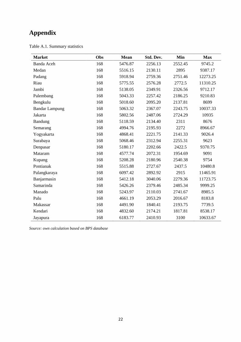
Appendix
Table A.1. Summary statistics
Market Obs Mean Std. Dev. Min Max
Banda Aceh 168 5476.87 2256.13 2552.45 9745.2
Medan 168 5516.15 2130.11 2895 9387.17
Padang 168 5918.94 2759.36 2751.46 12273.25
Riau 168 5775.55 2576.28 2772.5 11310.25
Jambi 168 5138.05 2349.91 2326.56 9712.17
Palembang 168 5043.33 2257.42 2186.25 9210.83
Bengkulu 168 5018.60 2095.20 2137.81 8699
Bandar Lampung 168 5063.32 2367.07 2243.75 10037.33
Jakarta 168 5802.56 2487.06 2724.29 10935
Bandung 168 5118.59 2134.40 2311 8676
Semarang 168 4994.76 2195.93 2272 8966.67
Yogyakarta 168 4868.41 2221.75 2141.33 9026.4
Surabaya 168 5068.46 2312.94 2255.31 9623
Denpasar 168 5180.17 2202.66 2422.5 9370.75
Mataram 168 4577.74 2072.31 1954.69 9091
Kupang 168 5208.28 2180.96 2540.38 9754
Pontianak 168 5515.88 2727.67 2437.5 10480.8
Palangkaraya 168 6097.42 2892.92 2915 11465.91
Banjarmasin 168 5412.18 3040.06 2279.36 11723.75
Samarinda 168 5426.26 2379.46 2485.34 9999.25
Manado 168 5243.97 2110.03 2741.67 8985.5
Palu 168 4661.19 2053.29 2016.67 8183.8
Makassar 168 4491.90 1840.41 2193.75 7739.5
Kendari 168 4832.60 2174.21 1817.81 8538.17
Jayapura 168 6183.77 2410.93 3100 10633.67
Source: own calculation based on BPS database