Food Marketing Policy Center

Estimation and Inference in Parametric Stochastic Frontier Models: A SAS/IML Procedure for a Bootstrap Method

by Sylvie Tchumtchoua

Food Marketing Policy Center Research Report No. 95

August 2006

Research Report Series http://www.fmpc.uconn.edu

University of Connecticut Department of Agricultural and Resource Economics

1

Estimation and Inference in Parametric Stochastic Frontier Models: A SAS/IML

Procedure for a Bootstrap Method

Sylvie Tchumtchoua

University of Connecticut Storrs

August 2006

Abstract

Parametric Stochastic Frontier Models are widely used in productivity analysis and are

commonly estimated using FRONTIER, STATA or LIMDEP packages, which only

provide point estimates for firm-specific technical efficiency. Confidence intervals for

technical efficiencies with superior coverage properties than those offered by the Horrace

and Schmidt (1996) method may be computed using the Bootstrap method introduced by

Simar and Wilson (2005). To facilitate these calculations, we propose a SAS/IML

procedure, which computes these confidence intervals for stochastic frontier models with

or without inefficiency effects. We apply the program to estimating supermarket-specific

technical efficiency in the U.S. Results indicates that the program works very well and

produce narrower confidence intervals than those obtain using Horrace and Schmidt

(1996) method.

2

1. Introduction

The parametric stochastic frontier model (PSFM) was introduced independently by

Aigner et al. (1977) and Meeusen and van den Broeck (1977) and has been extensively

used in productivity analysis (see Kumbhakar and Lovell, 2000 and references therein).

In this model the output of a production unit is specified in terms of a response function

and a composed error uv− , where v is a symmetric noise, and u is a nonnegative term

representing technical inefficiency. In applications, researchers are mainly interested in

point estimates and confidence intervals for the marginal effects and firm-specific

technical efficiency.

PSFM are commonly estimated by maximum likelihood method using either the

routine Frontier in LIMDEP or STATA, two general-purpose econometric packages, or

FRONTIER, a noncommercial special-purpose program (Sena, 1999; Herrero and

Pascoe, 2002). All of these packages have strengths and weaknesses. First, they provide

both point estimates and confidence intervals for the model quantities of interest, but only

point estimates of firm-specific and mean level technical efficiency. Second, although

FRONTIER has more analytical capabilities compared to LIMDEP, it is less user-

friendly. Third, none of the package allows the user to compute additional quantities

within the program and thus cannot be used in studies where the model likelihood

function has to be maximized repeatedly. In her review of FRONTIER and LIMPDEP

packages, Sena (1999) concludes that the ideal software would be one that combines their

strengths.

In this paper, we propose a program that addresses some of the shortcomings of

STATA, LIMDEP and FRONTIER with respect to estimation and inference of stochastic

3

frontier models. Our program computes confidence intervals for firm-specific technical

efficiency using a bootstrap method introduced by Simar and Wilson (2005), which make

inference about technical efficiency based on their sampling distribution. Previously

Horrace and Schmidt (1996) proposed an approach for inference about efficiency in

PSFM based on the percentiles of the estimated distribution of the one-sided error term,

conditional on the composite error, which is not the sampling distribution of the

inefficiency estimator.

The program is written using matrix language SAS/IML with the optimization

subroutine NLPQN. The program follows the step-by-step computational processes for

estimating PSFM by maximum likelihood, thus is more pedagogically useful, whereas

FRONTIER and the routine frontier in LIMDEP and STATA are in black boxes. In

addition, the program can be extended to various specifications of frontier models, or

simplified to a model without inefficiency effects.

We apply the program to the estimation of technical efficiencies in the U.S.

supermarket industry using a cross-section of 772 supermarkets in 2004.

The rest of the paper is organized as follows. Section 2 presents the model and derives

the likelihood function. Simar and Wilson (2005) bootstrap method is discussed in

section 3 and its SAS/IML implementation in section 4. Section 5 discusses some

extensions of the program. Application to U.S. supermarket industry follows in section 6

and section 7 concludes.

4

2. Model and likelihood function

We present the Battese and Coelli (1995) model which is the basic stochastic production

frontier model of Aigner et al. (1977) with technical inefficiency effects. The model for

cross-sectional data is given by

iiiiuvXy −+= β , i=1, …,N, (1)

where i

y represents the of logarithm of output for firm i; i

X is a k×1 vector of logarithm

of inputs of firm i, including a column of ones. This specification corresponds to the

Codd-Douglas production function. Other formulations such as Translog production

function are used in applications.

β is a 1×k vector representing marginal effects.

The i

v ’s are random noise and are independently and identically distributed as

),0( 2

vN σ and are independent from the

iu ’s. The

iu represent inefficiency and are assumed

independently distributed as a truncated (above zero) normal distribution with mean δi

Z

and variance 2

uσ , where

iZ is a (1xm) vector of firm-specific variables and δ a 1×m

vector of unknown coefficients of the firm-specific inefficiency variables.

Under the above assumptions and following Battese and Coelli (1995), the density

function of the composed error uveii

−= is given by

Φ

+

+

Φ+=

−

*

*

2/122

1

2/122

)()()(

σ

µ

σσ

δφ

σ

δσσ

vu

ii

u

i

vui

ZeZef (2)

where 2/122

*

)(vu

vu

σσ

σσσ

+= , and

22

22

*

vu

iuveZ

σσ

σδσµ

+

−= .

The model log likelihood on the basis of N observations is then given by

5

∑∑

∑

==

=

Φ−

Φ−++−−++−=

=

N

i

i

u

i

N

i

vuiiivu

N

i

ivu

ZZXy

N

efyL

1

*

*

1

22222

1

22

lnln)/()(2

1)ln(2(ln

2

))(ln();,,,(

σ

µ

σ

δσσδβσσπ

σσδβ

Using the re-parameterization involving the parameters 222

uvσσσ += and 22 /σσγ

u= , the

log likelihood function is expressed as

∑∑==

−

−−−Φ−

Φ−+−−+−=

N

i

iiii

N

i

iii

XyZZZXy

NyL

1

2/122/12

1

2222

))1((

)()1(ln

)(ln/)(

2

1)ln2(ln

2);,,,(

σγγ

βγδγ

γσ

δσδβσπγσδβ

(3)

Firm level technical efficiency is given by

+−

Φ

−Φ

=== − 2

*

*

*

*2

2

1exp]|[),,|,,,( σµ

σ

µ

σσ

µ

εγσδβττi

i

i

i

iu

iiiiieEyZX (4)

where iii

Z γεδγµ −−= )1( , 22

*)1( σγγσ −= , 222

vuσσσ += ,

2

2

σ

σγ u= , and Φ is the cumulative

density function of the standard normal distribution.

Using the data N

iiiiyZX

1)},,{(

=, the log likelihood in (3) must be maximized to obtain

estimates of the parameters β , δ , 2σ , γ which are then plug in (4) to get point estimates

of firm-specific technical efficiency N

ii 1}{

=τ . This is done automatically in STATA and

LIMDEP by using the routine frontier, or in FRONTIER by typing instructions

interactively on the screen or using an instruction file.

Horrace and Schmidt (1996) proposed an after-estimation formula for confidence

intervals of firm-specific technical efficiency. They compute a %100)1( α− confidence

interval for ]|[i

iu

ieE ετ −= as

( ))exp(,)exp( **

iUiiiLiizz σµσµ −−−−

6

where )}/()2/(1{ *1

iiLiz σµα Φ−Φ= − and )}/()2/1(1{ *1

iiUiz σµα Φ−−Φ= − . α is the nominal

size.

However, the above interval considers the parameters of the model to be known

and therefore do not reflect uncertainty about these parameters. As Wilson and Simar

(2005) pointed out, it is based on the percentile of the distribution of i

iue ε|−

, instead of the

sampling distribution of i

τ̂ .

3. Wilson and Simar bootstrap method

Wilson and Simar (2005) introduced a parametric bootstrap method which we modify to

incorporate the efficiency model; in their model the one sided error has a half normal

distribution whereas in our model we have a truncated normal distribution with mean

expressed as a function of firm-specific inefficiency variables. The method computes

confidence intervals for firm-specific technical efficiency using its sampling distribution.

It consists of the following steps:

(i) Using the data N

iiiinyZXD

1)},,{(

== , maximize the log-likelihood in (3) to obtain the

parameters β̂ , δ̂ , 2σ̂ , γ̂ ; recover 2ˆu

σ and 2ˆv

σ from 2σ̂ and γ̂ .

(ii) For i=1, …, N, draw )ˆ,0(~ 2*

viNv σ and )ˆ,ˆ(~ 2*

uiiZNu σδ+ , and compute *** ˆ

iiiiuvXy −+= β .

(iii) Using the pseudo-data n

iiiinyZXD

1

** )},,{(=

= , maximize (3) and obtain bootstrap

estimates *β̂ , *δ̂ , 2*σ̂ , *γ̂ , then compute ),,|ˆ,ˆ,ˆ,ˆ(ˆ *2****

iiiiyZXγσδβττ = , i=1,…,N.

(iv) Repeat (2) – (3) B times to obtain the bootstrap estimates

B

bibbB

1b

N

1i

**

b

*2

b

** }))}ˆ({ ,ˆ , ˆ , ˆ , ˆ {(==

= τγσδβ .

7

The bootstrap estimates are then used to compute the mean and percentiles of the

model parameters β , δ , 2σ , and γ , and each firm’s technical efficiency scores. The

percentiles can be used to compute 100×α % confidence intervals as

− )2

1()2

( ˆ,ˆαα

θθ where

)(ˆ αθ denotes the 100×α -percentile of B

bb 1

*}ˆ{=

θ , }ˆ ,ˆ , ˆ , ˆ , ˆ {ˆb

**

b

*2

b

***

ibbbτγσδβθ ∈ , α being the nominal

size. Note that standard software packages FRONTIER, LIMDEP and STATA do not

provide confidence interval for technical efficiency scores and rely on asymptotic

normality for inference about the parameter β and δ .

4. SAS/IML implementation of Wilson and Simar bootstrap method

The program listings in the appendix demonstrate the step-by-step computational process

for estimation of parametric stochastic frontier models based on the method of Wilson

and Simar. This method requires repeated maximization of the log-likelihood function

(3). Each maximization can only be done using nonlinear optimization methods.

SAS/IML provides all the pieces necessary to carry out the complete method. It is

a high-level matrix language for programming purposes that includes a set of build-in

nonlinear optimization subroutines for estimation of constrained and unconstrained

parameters through iterative process (SAS Institute, 2000). The SAS/IML program is

very flexible, thus giving the user control over all aspects of the maximum likelihood,

and the possibility to compute any quantity of interest.

The program consists of two macros: Maximize and bootstrap. We describe each

macro in turn.

8

4.1. Macro for maximizing the loglikelihood

Macro Maximize maximizes the log likelihood (3). We select the NLPQN subroutine that

uses the quasi-Newton optimization method as nonlinear optimization routine. The

arguments for the NLPQN are: the objective function module, the gradient module, the

starting values, the parameter constraints, the termination criteria, and the update method.

We discuss each of the argument in turn.

The objective function module “LL” specifies the function to be maximized (the

log likelihood function given by (3)). Its argument is theta, the column vector of the

parameters underlying the log likelihood function. Other quantities needed to evaluate LL

(the observed data) are passed to LL via the global function.

The module “GRAD” specifies the gradient function to compute the first-order

derivatives. The arguments and the quantities needed to evaluate the module are the same

as in LL. The first-order derivatives are given below:

'

1

2/12

2/12

2/12

2 ))1((

))1((

)()1(

))1((

)()1(

i

N

i iii

iii

iii XXyZ

XyZ

ZXyL∑

=

−

−

−−−Φ

−

−−−

++−

=∂

∂

σγγ

γ

σγγ

βγδγ

σγγ

βγδγφ

σ

δβ

β

'

1

2/12

2/12

2/12

2/12

2/12

2/12

2 ))1((

1

))1((

)()1(

))1((

)()1(

)(

1

)(

)(i

N

i iii

iii

i

i

iii ZXyZ

XyZ

Z

Z

ZXyL∑

=

−

−

−

−−−Φ

−

−−−

−

Φ

++−

−=∂

∂

σγγ

γ

σγγ

βγδγ

σγγ

βγδγφ

γσ

γσ

δ

γσ

δφ

σ

δβ

δ

9

−

−−−

−

−−−Φ

−

−−−

−

Φ

++−

−−=∂

∂∑

=

N

i

iii

iii

iii

i

i

i

iiiXyZ

XyZ

XyZ

Z

Z

Z

ZXyN

L

1

2/12

2/12

2/12

2/12

2/12

2/12

2

2

22))1((

)()1(

))1((

)()1(

))1((

)()1(

)(

)(

)()(

2

1

σγγ

βγδγ

σγγ

βγδγ

σγγ

βγδγφ

γσ

δ

γσ

δ

γσ

δφ

σ

δβ

σσ

∑

−−

−−−−+

−

+−

−

−−−Φ

−

−−−

−

Φ

=∂

∂2/122/12

2/12

2/12

2/12

2/12

2/12

))1()(1(2

)]()1)[(21(

))1((

))1((

)()1(

))1((

)()1(

)(2

)(

)(

σγγγγ

βγδγγ

σγγ

δβ

σγγ

βγδγ

σγγ

βγδγφ

γσγ

δ

γσ

δ

γσ

δφ

γiiiiii

iii

iii

i

i

i

XyZZXy

XyZ

XyZ

Z

Z

Z

L

The gradient module is not required in the NLPQN subroutine and when it is not

specified, the NLPQN subroutine uses numerical approximations of the gradient vector

by the finite difference method. But, it usually requires more calls to the function module

for the iterative process to converge. It is better to use these analytic derivatives if they

are available instead of relying on finite difference approximations.

We define the starting values of the iteration process as in Coelli (1994). The OLS

estimates are obtained and a grid search procedure is used to obtain a starting value for γ .

The parameter constraints are specified in the input argument con, which is a

)2(2 ++× mk matrix (the model has k parameters in β , m in δ , and two additional

parameters 2σ and γ ). The first row and second row define the lower and upper bounds

respectively. Except for γ and 2σ all the other elements of the matrix are specified as

missing values. γ and 2σ are constrained with a lower bound of 8101 −× to prevent their

becoming zero or negative. The upper bound of γ is 1.

The input argument ter specifies a vector of bounds corresponding to a set of

termination criteria that are tested in each iteration and determine when the optimization

process stops. Stopping criterion selected is 51)max( −< egradient . The first three

components of ter vector are set to missing values to allow use of the default values.

10

Following Coelli (1994), we specify the original Davidon, Fletcher, and Powell

(DFP) (option [4] =4) as update method for the inverse Hessian matrix. The DFP method

performs a line search in each iteration on the search direction with quadratic

interpolation and cubic extrapolation.

A call of the NLPQN subroutine returns tow results. The first one is a number rc,

which, when positive, indicates that the iteration process has terminated successfully with

one of the specified criteria, and when negative indicates unsuccessful termination. The

second result is a vector xr of length equal to the length of the starting values matrix,

which contains the optimal values when 0>rc . These optimal values are then used to

compute firm-specific technical efficiency scores using (4), to draw values for *

iv , *

iu , to

compute pseudo dependent variable *

iy , for i=1,…,N as described in step (ii) in the

method, and to form the pseudo data n

iiiinyZXD

1

** )},,{(=

= .

4.2. The macro for estimation of confidence intervals

Macro bootstrap estimates the confidence intervals of marginal effects and firm-specific

technical efficiency by bootstrapping. It follows the four steps of Wilson and Simar

algorithm outlined above. First it uses the original data to maximize the log-likelihood

function and obtain initial parameters estimates. Second, these initial parameter estimates

are used to draw the error terms (noise and inefficiency term) and compute the pseudo-

data. Third, the pseudo-data are used to maximize the log-likelihood function using

macro Maximize and obtain Bootstrap estimates. Fourth, steps 1-3 are repeated B times,

where B is the number of Bootstrap replications.

11

Input for this macro consists of the SAS dataset put in the format described

below, the number of production inputs, the number of inefficiency variables, and the

number of bootstrap replications. The macro returns

Testing for the presence of technical inefficiencies in the data using likelihood-

ratio test is straightforward using the program. Following Battese and Coelli (1995), the

null hypothesis is 0:10

====m

H δδγ L . The likelihood ratio test statistic is calculated as

)}(log)({log210

HlikelihoodHlikelihoodLR −−=

where )(log0

Hlikelihood and )(log1

Hlikelihood are the values of the log likelihood function

under the null and the alternative hypothesis, respectively.

Under 0

H , LR has an asymptotic distribution which is a mixture of chi-square

distributions, namely 2

1

1

02

1

2

1χχ + (Coelli, 1995).

How to use the SAS/IML procedure

The program listing is given in the appendix. It is very easy to use; all the user has to do

is to put the data in the following format:

1 y1 x11…x1k z11…z1m

2 y2 x21…x2k z21…z2m

. . . . . .

N yN xN1…xNk zN1…zNm

where the first column list the N firms, the second column represents firms’ outputs, the

next k columns represent the k inputs and the last m columns represents the m possible

determinants of technical efficiency.

After importing the data as

12

proc import datafile="C:\data.xls"

out=data replace;

run;

the procedure is called using

%Bootstrap (dsn=data, K=k, M=m, B=b).

5. Extensions

The SAS/IML program presented in appendix can easily be extended in many ways. For

panel data, all the user has to do is to specify the appropriate log likelihood function and

derive the corresponding first-order derivatives. The specification of the composed errors

can be extended to incorporate heteroscedasticity in both the symmetric component and

the one-sided component as in Hadri et al. (2003). In the presence of heteroscedasticity,

the variances of i

u and i

v are not constant across observations. Following Hadri (1999)

and Hadri et al. (2003), heteroscedasticity can be incorporated multiplicatively by

specifying the variances of the error components as )exp( ρσivi

V= , and )exp( ϕσiui

W= ,

where i

V and i

W are vectors of nonstochastic explanatory variables the researcher

believes explain differences in variances across observations. In the presence of

heteroscedasticity, the log likelihood function in (3) is still appropriate, except that the

variances are replaced by their new expressions.

6. Application

We apply the program to the estimation of technical efficiency in U.S. supermarket

industry. Data came from the Trade Dimension database at the Food Marketing Policy

13

Center at the University of Connecticut. It consists of 772 supermarkets (not including

Wall-Mart) in the U.S. in 2004. Additional information on socio-demographic

characteristics was obtained from the U.S. Census bureau web page. Output is measured

by the average weekly dollar sales. We consider two inputs: labor measured by the

number of full time and part time equivalent employees, and capital by the area of selling

space. As possible determinants of technical efficiency, we use dummy variables of

whether s store belongs to a chain, has a pharmacy department or sells liquor.

Using the SAS/IML program, we compute B=500 bootstrap estimates of the model

parameters and technical efficiencies. Running the 500 bootstrap replications took 22

minutes on a 2.40 GHz Pentium 4 processor. Table 1 displays the mean, standard

deviation, 5% and 95% percentiles of the model parameters. We also display in table 2

estimates of means and standard deviations obtained using FRONTIER, STATA, and

SAS/IML side by side. It appears that the two sets of estimates are approximately the

same.

Figure 1 plots SAS/IML point estimates and 95% confidence intervals of the ranked

values efficiency scores. It appears that technical efficiencies are estimated with moderate

precision as indicated by the relatively narrow 95% confidence intervals.

Figure 2 plots confidence intervals for technical efficiency using Horrace and

Schmidt (1996) method. Compared to the Bootstrap estimates, Horrace and Schmidt

confidence intervals are wider. This may be due to the fact that they do not take into

account uncertainty about the parameters of the model.

14

7. Conclusion

In this paper we have proposed a SAS/IML program for estimation and inference in

parametric stochastic frontier models. The program is useful to practitioners for many

reasons. First, it computes point estimates and statistically sound confidence interval

estimates for firm-specific technical efficiency whereas commonly available software

packages do not have built in commands for obtaining confidence intervals for technical

efficiency. Second, the program is pedagogically very useful as it demonstrates the step-

by-step estimation process. Third, the program is very flexible and can be extended to

various specifications of stochastic frontier model. Fourth, researchers may find the

program useful in conducting Monte Carlo studies to investigate the properties of

stochastic frontier methods that involve numerical optimization.

15

References

Aigner, D.J. Lovell, C.A.K., Schmidt, P. (1977). ‘Formulation and estimation of

stochastic frontier production models.’ Journal of Econometrics 12:21-37.

Battese, G.E., & Coelli, T.J. (1992). ‘Frontier production functions, technical efficiency

and panel data with application to paddy farmers in India.’ Journal of productivity

analysis 3: 153-169.

Battese, G.E., & Coelli, T.J. (1995). ‘A model for technical efficiency effects in a

stochastic frontier production function for panel data.’ Empirical economics 20;

325-332.

Coelli, T.J. (1994). ‘A Guide to FRONTIER Version 4.1: A Computer Program for

Stochastic Frontier Production and Cost Function Estimation.’ CEPA Working

Paper 96/07.

Coelli, T.J. (1995). ‘Estimators and hypothesis tests for a stochastic frontier function: A

Monte Carlo analysis.’ Journal of productivity analysis 6: 247-268.

Hadri, K., Guermat, C., & Whittaker, J. (2003). ‘Estimation of technical inefficiency

effects using panel data and doubly heteroscedastic stochastic production

frontiers.’ Empirical Economics 28: 203-222.

Hadri, K. (1999). ‘Estimation of a doubly heteroscedastic stochastic frontier cost

function.’ Journal of Business and Economic Statistics 17:257-282.

Herrero, L., & Pascoe, S. (2002). ‘Estimation of technical efficiency: A review of some

of the stochastic frontier and DEA software.’ Computers in Higher education

economics review. Virtual Edition (http://www.economics.ltsn.ac.uk/cheers.htm).

16

Horrace W.C. & Schmidt, P. (1996). ‘Confidence statements for efficiency estimates

from stochastic frontier models.’ Journal of productivity analysis 7: 257-282.

Kumbhakar, S.C. Lovell, C.A.K. (2000). Stochastic frontier analysis. New York:

Cambridge University Press.

Meeusen, W., van den Broeck, J. (1977). ‘Efficiency estimation from Cobb-Douglas

production functions with composed errors’. International Economic Review

8:435-444.

SAS Institute. (2000). ‘SAS/IML user’s guide, version 8.’ Cary, NC: Author.

Sena, V. (1999). Stochastic Frontier Estimation: a review of the software options. Journal

of Applied Econometrics 14: 579-586.

Simar, L. & Wilson, P.W. (2005). Estimation and inference in cross-sectional, stochastic

Frontier Models.

17

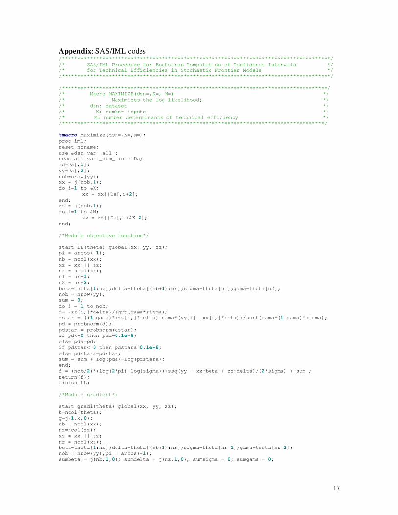
Appendix: SAS/IML codes /**************************************************************************************/

/* SAS/IML Procedure for Bootstrap Computation of Confidence Intervals */

/* for Technical Efficiencies in Stochastic Frontier Models */

/**************************************************************************************/

/*************************************************************************************/

/* Macro MAXIMIZE(dsn=,K=, M=) */

/* Maximizes the log-likelihood; */

/* dsn: dataset */

/* K: number inputs */

/* M: number determinants of technical efficiency */

/************************************************************************************/

%macro Maximize(dsn=,K=,M=);

proc iml;

reset noname;

use &dsn var _all_;

read all var _num_ into Da;

id=Da[,1];

yy=Da[,2];

nob=nrow(yy);

xx = j(nob,1);

do i=1 to &K;

xx = xx||Da[,i+2];

end;

zz = j(nob,1);

do i=1 to &M;

zz = zz||Da[,i+&K+2];

end;

/*Module objective function*/

start LL(theta) global(xx, yy, zz);

pi = arcos(-1);

nb = ncol(xx);

xz = xx || zz;

nr = ncol(xz);

n1 = nr+1;

n2 = nr+2;

beta=theta[1:nb];delta=theta[(nb+1):nr];sigma=theta[n1];gama=theta[n2];

nob = nrow(yy);

sum = 0;

do i = 1 to nob;

d= (zz[i,]*delta)/sqrt(gama*sigma);

dstar = ((1-gama)*(zz[i,]*delta)-gama*(yy[i]- xx[i,]*beta))/sqrt(gama*(1-gama)*sigma);

pd = probnorm(d);

pdstar = probnorm(dstar);

if pd<=0 then pda=0.1e-8;

else pda=pd;

if pdstar<=0 then pdstara=0.1e-8;

else pdstara=pdstar;

sum = sum + log(pda)-log(pdstara);

end;

f = (nob/2)*(log(2*pi)+log(sigma))+ssq(yy - xx*beta + zz*delta)/(2*sigma) + sum ;

return(f);

finish LL;

/*Module gradient*/

start gradi(theta) global(xx, yy, zz);

k=ncol(theta);

g=j(1,k,0);

nb = ncol(xx);

nz=ncol(zz);

xz = xx || zz;

nr = ncol(xz);

beta=theta[1:nb];delta=theta[(nb+1):nr];sigma=theta[nr+1];gama=theta[nr+2];

nob = nrow(yy);pi = arcos(-1);

sumbeta = j(nb,1,0); sumdelta = j(nz,1,0); sumsigma = 0; sumgama = 0;

18

do i = 1 to nob;

es = (yy[i]- xx[i,]*beta + zz[i,]*delta)/sigma;

es2=(yy[i]- xx[i,]*beta + zz[i,]*delta)*(yy[i]- xx[i,]*beta + zz[i,]*delta)/sigma;

dstar = ((1-gama)*(zz[i,]*delta)-gama*(yy[i]-xx[i,]*beta))/sqrt(gama*(1-gama)*sigma);

cdfdstar = probnorm(dstar);

pdfdstar = (1/sqrt(2*pi))*exp(-dstar*dstar/2);

d = (zz[i,]*delta)/sqrt(gama*sigma);

cdfd = probnorm(d);

pdfd = (1/sqrt(2*pi))*exp(-d*d/2);

sigmastar=sqrt(gama*(1-gama)*sigma);

sumbeta = sumbeta+(es + (gama/sigmastar)*pdfdstar/cdfdstar)*xx[i,]`;

sumdelta = sumdelta-(es + (pdfd/cdfd)/sqrt(gama*sigma)-(pdfdstar/cdfdstar)*((1-

gama)/sigmastar))*zz[i,]`;

sumsigma = sumsigma -(1/(2*sigma))*(1-es2 -((pdfd/cdfd)*d - (pdfdstar/cdfdstar)*dstar));

sumgama = sumgama+(pdfd/cdfd)*d/(2*gama)-(pdfdstar/cdfdstar)*((yy[i]-

xx[i,]*beta+zz[i,]*delta)/sigmastar +(1-2*gama)*dstar/(2*gama*(1-gama)));

end;

g[1,1:nb]=-sumbeta`;

g[1,(nb+1):nr]=-sumdelta`;

g[1,nr+1]=-sumsigma;

g[1,nr+2]=-sumgama;

return(g);

finish gradi;

/*Grid search for starting values*/

* Ordinary least squares estimates;

nb = ncol(xx);

ob1 = inv(xx`*xx)*xx`*yy;

e = yy - xx*ob1;

sigma2 = ssq(e)/(nob-nb);

*Grid search for gamma;

ob = j(1,nb+1,0);

ob[1:nb]=ob1;

ob[nb+1]=sigma2;

pi = arcos(-1);

nob = nrow(yy);

xz = xx || zz;

nb = ncol(xx);

nr = ncol(xz);

n1 = nr +1;

n2 = nr + 2;

theta0 = j(1,n2,0);

y = j(1,n2,0);

x = j(1,n2,0);

var=ob[nb+1]*(nob-nb)/nob;

b0 = ob[1];

do i=1 to nb;

y[i] = ob[i];

end;

do i= nb+1 to nr;

y[i]=0;

end;

fx = 1e+16;

gridno = 0.1;

y6b=gridno;

y6t=1.0-gridno;

do y6= y6b to y6t by gridno;

y[n2]=y6;

y[n1]= var/(1-2*y[n2]/pi);

c=(y[n2]*y[n1]*2/pi)**0.5;

y[1]=b0+c;

f = LL(y);

if f < fx then do;

fx=f;

do i=1 to n2;

x[i] = y[i];

19

end;

end;

end;

do i =1 to n2;

theta0[i]=x[i];

end;

/*Options and parameters constraints*/

ter = j(1,13,.);

ter[1]=4000; ter[2]=4000; ter[3]=.; ter[6]=1e-5;ter[9]=0;

ter[4]=0; ter[5]=0; ter[7]=0; ter[8]=0;

ter[11]=1e-5; ter[12]=0; ter[13]=1e-5;

con=j(2,&K+&M+4,.);

con[1,&K+&M+3]=1e-18; con[2,&K+&M+4]=1;

option = {0 2 . 4};

call nlpqn(rc,xr,"LL",theta0,option,con)grd="gradi" tc=ter;

create opt from xr;

append from xr;

close opt;

if rc >0 then print '*The iterative process terminates successfully*';

else print '*Warning: unsuccessful termination*';

quit;

%mend;

/*************************************************************************************/

/* Macro BOOTSTRAP(dsn=,K=, M=, B=) */

/* Computes bootstap estimates */

/* dsn: dataset */

/* K: number inputs */

/* M: number determinants of technical efficiency */

/* B: number bootstrap replications */

/*************************************************************************************/

%macro Bootstrap(dsn=,K=,M=,B=);

/*Use original data to maximize the log-likelihood and obtain initial parameter and

technical efficiencies estimates*/

%Maximize(dsn=&dsn,K=&K,M=&M);

proc iml;

use opt var _all_;

read all var _num_ into Pa;

beta=Pa[1:&K+1]; delta=Pa[&K+2:&K+&M+2];sigma2=Pa[&K+&M+3];gama=Pa[&K+&M+4];

sigmau=gama*sigma2;

sigmav=sigma2*(1-gama);

param=beta`||delta`||sigmau||sigmav||gama;

create paramet from param;

append from param;

close paramet;

create parameters from param;

append from param;

close parameters;

use &dsn var _all_;

read all var _num_ into Da;

id=Da[,1];

yy=Da[,2];

nob=nrow(yy);

xx = j(nob,1);

do i=1 to &K;

xx = xx||Da[,i+2];

end;

zz = j(nob,1);

do i=1 to &M;

zz = zz||Da[,i+&K+2];

end;

te = j(nob,1,0.);

20

do i = 1 to nob;

zd=zz[i,]*delta;

xb=xx[i,]*beta;

us = (1-gama)*zd-gama*(yy[i]-xb);

ss = (gama*(1-gama)*sigma2)**0.5;

ds=us/ss;

te[i] = exp(-us+0.5*ss**2)*probnorm(ds-ss)/probnorm(ds);

end;

tei=id||te;

create efficiency from tei;

append from tei;

close efficiency;

quit;

/*Repeatedly create pseudo-data and use them to maximize the log-likelihood*/

%do i=1 %to &B;

proc iml;

/*Create pseudo data*/

use paramet var _all_;

read all var _num_ into Par;

beta=Par[1:&K+1];

delta=Par[&K+2:&K+&M+2]; sigmau=Par[&K+&M+3]; sigmav=par[&K+&M+4];

gama=par[&K+&M+5];

use &dsn var _all_;

read all var _num_ into Da;

id=Da[,1];

yy=Da[,2];

nob=nrow(yy);

xx = j(nob,1);

do i=1 to &K;

xx = xx||Da[,i+2];

end;

zz = j(nob,1);

do i=1 to &M;

zz = zz||Da[,i+&K+2];

end;

v=j(nob,1,0.);

u=j(nob,1,0.);

yys=j(nob,1,0.);

do i =1 to nob;

seed=-i;

v[i]=(sqrt(sigmav))*rannor(seed);

u[i]=zz[i,]*delta+(sqrt(sigmau))*rannor(seed);

do while (u[i]<0);

u[i]=zz[i,]*delta+(sqrt(sigmau))*rannor(seed);

end;

yys[i]=xx[i,]*beta+v[i]-u[i];

end;

pseudo=id||yys||xx[,2:&K+1]||zz[,2:&M+1];

create pdata from pseudo;

append from pseudo;

close pdata;

quit;

/*Use pseudo-data to maximize the likelihood*/

%Maximize(dsn=pdata,K=&K,M=&M);

/*Save parameters Boostrap estimates*/

proc iml;

use opt var _all_;

read all var _num_ into Pab;

beta=Pab[1:&K+1]; delta=Pab[(&K+2):&K+&M+2];

gama=Pab[&K+&M+4];sigma2=Pab[&K+&M+3];

sigmau=gama*sigma2;

sigmav=sigma2*(1-gama);

par=beta`||delta`||sigmau|| sigmav|| gama;

edit parameters;

append from par;

run;

21

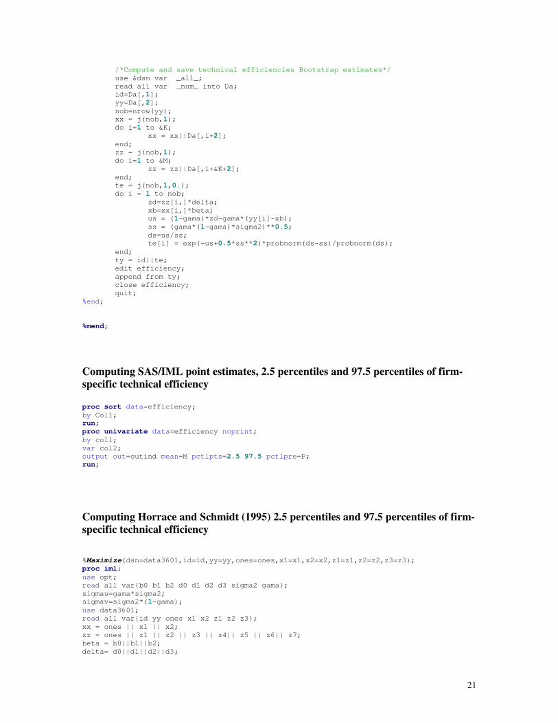
/*Compute and save technical efficiencies Bootstrap estimates*/

use &dsn var _all_;

read all var _num_ into Da;

id=Da[,1];

yy=Da[,2];

nob=nrow(yy);

xx = j(nob,1);

do i=1 to &K;

xx = xx||Da[,i+2];

end;

zz = j(nob,1);

do i=1 to &M;

zz = zz||Da[,i+&K+2];

end;

te = j(nob,1,0.);

do i = 1 to nob;

zd=zz[i,]*delta;

xb=xx[i,]*beta;

us = (1-gama)*zd-gama*(yy[i]-xb);

ss = (gama*(1-gama)*sigma2)**0.5;

ds=us/ss;

te[i] = exp(-us+0.5*ss**2)*probnorm(ds-ss)/probnorm(ds);

end;

ty = id||te;

edit efficiency;

append from ty;

close efficiency;

quit;

%end;

%mend;

Computing SAS/IML point estimates, 2.5 percentiles and 97.5 percentiles of firm-

specific technical efficiency

proc sort data=efficiency;

by Col1;

run;

proc univariate data=efficiency noprint;

by col1;

var col2;

output out=outind mean=M pctlpts=2.5 97.5 pctlpre=P;

run;

Computing Horrace and Schmidt (1995) 2.5 percentiles and 97.5 percentiles of firm-

specific technical efficiency

%Maximize(dsn=data3601,id=id,yy=yy,ones=ones,x1=x1,x2=x2,z1=z1,z2=z2,z3=z3);

proc iml;

use opt;

read all var{b0 b1 b2 d0 d1 d2 d3 sigma2 gama};

sigmau=gama*sigma2;

sigmav=sigma2*(1-gama);

use data3601;

read all var{id yy ones x1 x2 z1 z2 z3};

xx = ones || x1 || x2;

zz = ones || z1 || z2 || z3 || z4|| z5 || z6|| z7;

beta = b0||b1||b2;

delta= d0||d1||d2||d3;

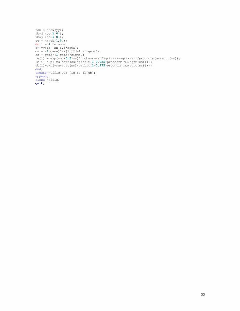
22

nob = nrow(yy);

lb=j(nob,1,0.);

ub=j(nob,1,0.);

te = j(nob,1,0.);

do i = 1 to nob;

e= yy[i]- xx[i,]*beta`;

mu = (1-gama)*zz[i,]*delta`-gama*e;

ss = gama*(1-gama)*sigma2;

te[i] = exp(-mu+0.5*ss)*probnorm(mu/sqrt(ss)-sqrt(ss))/probnorm(mu/sqrt(ss));

lb[i]=exp(-mu-sqrt(ss)*probit(1-0.025*probnorm(mu/sqrt(ss))));

ub[i]=exp(-mu-sqrt(ss)*probit(1-0.975*probnorm(mu/sqrt(ss))));

end;

create heffic var {id te lb ub};

append;

close heffic;

quit;

23

Table 1. Parameter estimates from SAS/IML program

Variables Coefficient Mean Std. deviation 2.5%

percentile

97.5%

percentile

Constant 0

β 7.494 0.331 6.831 8.123

Log Labor 1

β 0.307 0.020 0.349 0.476

Log Selling space 2

β 0.408 0.031 0.270 0.342

Constant 0

δ 0.655 0.121 0.408 0.885

Chain 1

δ -0.786 0.477 -1.306 -0.483

Pharmacy 3

δ -0.446 0.197 -0.936 -0.183

Liquor 4

δ 0.113 0.091 -0.055 0.297

2

uσ 0.095 0.030 0.047 0.161

2

vσ 0.069 0.011 0.046 0.089

γ 0.568 0.101 0.364 0.731

24

Table 2. Parameter estimates from FRONTIER, STATA, and SAS/IML

FRONTIER/STATA SAS/IML

Variables Mean Std.

deviation

Mean Std.

deviation

Constant 0

β 7.524 0.338 7.494 0.331

Log Labor 1

β 0.305 0.022 0.307 0.020

Log Selling space 2

β 0.406 0.032 0.408 0.031

Constant 0

δ 0.684 0.096 0.655 0.121

Chain 1

δ -0.729 0.150 -0.786 0.477

Pharmacy 3

δ -0.408 0.131 -0.446 0.197

Liquor 4

δ 0.104 0.085 0.113 0.091

2

uσ 0.098 0.028 0.095 0.030

2

vσ 0.070 0.009 0.069 0.011

γ 0.583 0.087 0.568 0.101

25

0

0.1

0.2

0.3

0.4

0.5

0.6

0.7

0.8

0.9

1T

echnic

al e

ffic

iency s

core

s

SAS/IML Point estimates SAS/IML 2.5 Pctiles

SAS/IML 97.5 Pctiles STATA/FRONTIER Point estimates

Figure 1. SAS/IML Technical efficiency scores

0

0.1

0.2

0.3

0.4

0.5

0.6

0.7

0.8

0.9

1

Te

ch

nic

al e

ffic

ien

cy s

co

res

Point estimates 2.5 Pctiles 97.5 Pctiles

Figure 2. Technical efficiency scores using Horrace and Schmidt (1996) formulas

FOOD MARKETING POLICY CENTER RESEARCH REPORT SERIES

This series includes final reports for contract research conducted by Policy Center Staff. The series also contains research direction and policy analysis papers. Some of these reports have been commissioned by the Center and are authored by especially qualified individuals from other institutions. (A list of previous reports in the series is available on our web site.) Other publications distributed by the Policy Center are the Working Paper Series, Journal Reprint Series for Regional Research Project NE-165: Private Strategies, Public Policies, and Food System Performance, and the Food Marketing Issue Paper Series. Food Marketing Policy Center staff contribute to these series. Individuals may receive a list of publications in these series and paper copies of older Research Reports are available for $20.00 each, $5.00 for students. Call or mail your request at the number or address below. Please make all checks payable to the University of Connecticut. Research Reports can be downloaded free of charge from our web site given below.

Food Marketing Policy Center 1376 Storrs Road, Unit 4021

University of Connecticut Storrs, CT 06269-4021

Tel: (860) 486-1927

FAX: (860) 486-2461 email: fmpc@uconn.edu

http://www.fmpc.uconn.edu